August 1996

Avoiding the Pitfalls:Can Regime-Switching Tests Detect Bubbles?

Simon van NordenE-mail: svannorden@bank-banque-canada.ca

International Department, Bank of CanadaOttawa, Ontario, Canada K1A 0G9

Robert VigfussonE-mail: rvigfusson@bank-banque-canada.caInternational Department, Bank of Canada

Ottawa, Ontario, Canada K1A 0G9

While retaining sole responsibility for any errors or oversights, the authors would like tothank their colleagues at the Bank of Canada for their comments and suggestions.

ISSN 1192-5434ISBN 0-662-25019-2

Printed in Canada on recycled paper

This paper is intended to make the results of Bank research available in preliminary formto other economists to encourage discussion and suggestions for revision. The viewsexpressed are those of the author. No responsibility for them should be attributed to theBank of Canada.

Abstract

Work on testing for bubbles has caused much debate, much of which has focussed onmethodology. Monte Carlo simulations reported in Evans (1991) showed that standardtests for unit roots and cointegration frequently reject the presence of bubbles even whensuch bubbles are present by construction. Evans referred to this problem as the pitfall oftesting for bubbles.

Since Evans' note, new tests for rational speculative bubbles that rely on regime-switchinghave been proposed. Van Norden and Schaller (1993) and van Norden (1996) use a switch-ing regression to look for a time-varying relationship between returns and deviations froman approximate fundamental price. Hall and Sola (1993) and Funke, Hall and Sola (1994)test whether asset prices seem to switch between explosive growth and stationary behav-iour.

Our paper reports on Monte Carlo experiments using Evans’ data-generating process togauge the performance of these two kinds of regime-switching tests. The experiments relyheavily on certain new, fast and robust programs developed at the Bank of Canada for theestimation of switching regression models that make Monte Carlo studies of such estima-tors practical. We find that for some (but not all) parameter values, regime-switching testshave a significant amount of power to detect periodically collapsing bubbles. We alsocompare and contrast the performance of the two different regime-switching tests.

Résumé

La mise au point de tests de détection des bulles spéculatives a occasionné bien des débats,principalement sur des points de méthodologie. Evans (1991) a démontré, au moyen desimulations de Monte-Carlo, que la présence de bulles est fréquemment rejetée par lestests standard de racine unitaire et de cointégration même quand des bulles ont été incor-porées à la construction des données. Ce problème constitue, à ses yeux, la pierred’achoppement de ce type de tests de détection des bulles.

Depuis la parution de l’article d’Evans, on a proposé de nouveaux tests de détection desbulles spéculatives rationnelles qui s’appuient sur un changement de régime. van Nordenet Schaller (1993) et van Norden (1996) ont eu recours à une régression avec changementde régime afin d’établir s’il existe une relation, variable dans le temps, entre les rende-ments et les écarts observés par rapport à un prix fondamental approximatif. De leur côté,Hall et Sola (1993) et Funke, Hall et Sola (1994) ont cherché à déterminer si le prix desactifs oscille entre une croissance explosive et un état stationnaire.

Dans la présente étude, les auteurs évaluent la puissance de ces deux types de tests aumoyen de simulations de Monte-Carlo; ils emploient pour cela le processus générateur dedonnées qu’utilise Evans. Leurs simulations font appel aux nouveaux programmes rapideset éprouvés mis au point à la Banque du Canada pour l’estimation des modèles de régres-sion avec changement de régime, lesquels rendent possible l’étude de tels estimateurs aumoyen de simulations. Les auteurs constatent que pour certaines valeurs paramétriques(mais pas pour toutes), les tests de régression avec changement de régime sont suffisam-ment puissants pour déceler les bulles qui s’effondrent périodiquement. Enfin, ils compar-ent la performance des deux tests afin d’en faire ressortir les similarités et les différences.

Contents

1.0 Introduction..............................................................................................................1

2.0 Tests for Rational Speculative Bubbles....................................................................22.1 Bubbles and Regime-Switching...........................................................................................2

2.2 The Hall and Sola Test for Bubbles .....................................................................................4

2.3 Van Norden Bubble Test ......................................................................................................5

2.4 Comparing Hall and Sola’s Test with van Norden’s Test ....................................................8

3.0 Experimental Design................................................................................................9

4.0 Monte Carlo Results ..............................................................................................134.1 Overview of Results...........................................................................................................13

4.2 Convergence.......................................................................................................................14

4.3 Hall and Sola Test ..............................................................................................................15

4.4 Van Norden Bubble Test ....................................................................................................17

4.5 Comparing van Norden and Hall and Sola. .......................................................................21

5.0 Conclusions............................................................................................................21

6.0 Bibliography ..........................................................................................................23

1

1.0 Introduction

Work on testing for rational speculative bubbles in financial markets has prompted muchdebate, much of which has focussed on methodology. Early work used variance-boundtests, until various econometric problems with this approach were noted (see LeRoy1989). The misspecification test suggested by West (1987) has fallen out of favour, sincemisspecified fundamentals should cause it to detect bubbles and there is little agreementon how to specify the fundamentals. (For example, see Flood and Hodrick 1990.) Dibaand Grossman (1988) and Hamilton and Whiteman (1985) recommend the use of tests forstationarity and for cointegration to test for the absence of rational speculative bubbles.However, Monte Carlo simulations reported in Evans (1991) show that standard tests forunit roots and cointegration frequently reject the presence of bubbles even when such bub-bles are present by construction.1 Evans refers to this problem as the “pitfall” of testing forbubbles.

Since Evans' note, new tests for rational speculative bubbles that rely on regime-switchinghave been proposed. Van Norden and Schaller (1993a, 1993b) and van Norden (1996) usea switching regression to look for a time-varying relationship between returns and devia-tions from an approximate fundamental price. Hall and Sola (1993) and Funke, Hall andSola (1994) test whether asset prices seem to switch between explosive growth and sta-tionary behaviour.

A potential flaw of this new approach is that the regime-switching estimators may not bewell behaved. There are two plausible grounds for concern.2

• The presence of rational speculative bubbles implies that the data are non-stationary,but the properties of regime-switching estimators in this instance are unknown. Sincethis non-stationarity exists only under the alternative hypothesis of bubbles, this raisesthe question of whether the regime-switching tests have the power to detect bubbleswhen they exist. This is similar to the pitfall that Evans (1991) found with the unit-rootand cointegration tests.3

• Little is known about the finite-sample properties of regime-switching estimators. Inparticular, little has been done to determine whether the use of tests whose distributionis known only asymptotically leads to reliable inference. It is conceivable that asymp-totically correct tests could experience size distortion in small samples, which wouldtend to produce evidence of speculative bubbles even when none is present.

1. Charemza and Deadman (1995) show that this problem extends to a broader range of processes than thoseconsidered by Evans (1991).

2. The problems of directly testing for the presence of regime-switching have recently become better under-stood. However, both of the above approaches circumvent these complications by testing a regime-switchingalternative against a regime-switching null.

3. Both problems could lead us to conclude that bubbles are absent when they are in fact present. The differ-ence is that, with the cointegration and unit-root tests, this result is caused by size distortion while with theregime-switching tests it is caused by a lack of power. This difference arises because the two kinds of testsreverse the null and alternative hypotheses.

2

Our paper is a first step in addressing these questions. We examine the power properties ofregime-switching bubble tests by carrying out Monte Carlo experiments using Evans’data-generating process (DGP). Our work relies on certain new, fast and robust programsdeveloped at the Bank of Canada (van Norden and Vigfusson 1996) for the estimation ofswitching regression models that make Monte Carlo studies of such estimators practical.We find that for some (but not all) parameter values, regime-switching tests have signifi-cant amount of power to detect periodically collapsing bubbles. We are also the first tocompare and contrast the performance of the two different kinds of regime-switchingtests.

In the following section, we explain the relationship between speculative bubbles andregime-switching, and then review the tests proposed by Hall and Sola and by van Norden.Section 3 explains the design of our Monte Carlo experiments, and their results are dis-cussed in Section 4. Section 5 concludes and gives several suggestions for furtherresearch.

2.0 Tests for Rational Speculative Bubbles

This section has three goals. We first describe what a bubble is. We next describe the tworegime-switching tests used in this paper to detect bubbles. Finally, we compare the twotests looking for similarities and differences.

2.1 Bubbles and Regime-Switching

Consider a simple asset-pricing model, which only requires that

(EQ 1)

where is the logarithm of the asset price, is the operator for expectations conditional

on information at timet, , and is a vector of other variables. Solving the

equation forward gives the general result

. (EQ 2)

One solution to equation (EQ 1), which we will denote , occurs when

, (EQ 3)

so

pt f Xt( ) a Et pt 1+( )⋅+=

pt Et

0 a 1< < Xt

pt a j Et f Xt j+( )( )⋅j 0=

T

∑

aT 1+ Et pT 1+( )⋅+=

pt*

aT 1+ Et pT 1+( )⋅T ∞→lim 0=

3

. (EQ 4)

We refer to (EQ 4) as the fundamental solution, since it determines the asset price solely asa function of the current and expected behaviour of other variables.

However, equation (EQ 4) is not the only solution to (EQ 1). We define bubble solutions tobe any other set of asset prices and expected asset prices that satisfy equation (EQ 1) but

where . We define the size of the bubble as

. (EQ 5)

Note that since satisfies equation (EQ 1), it follows4 from (EQ 1) and (EQ 5) that

. (EQ 6)

Since , this means the bubble must be expected to grow over time.5

Nothing in the above model has any implications for regime-switching. Some of the earlyliterature on rational speculative bubbles even considered purely deterministic bubbles.Regime-switching stems from the descriptions of asset market behaviour (for example,those surveyed in Kindleberger 1989) to which the above model of bubbles is oftenapplied. The first example of regime-switching in the rational speculative bubble frame-work is Blanchard (1979), who proposes a bubble that moves randomly between twostates,C andS. In stateC, the bubble will collapse, so6

. (EQ 7)

4. Blanchard (1979) has a more complete derivation of this and subsequent steps found in this section.

5. A considerable literature exists on the conditions under which such bubbles are feasible rational-expecta-tions solutions. Important contributions to this debate include Obstfeld and Rogoff (1983, 1986), Diba andGrossman (1987), Tirole (1982, 1985), Weil (1990), Buiter and Pesenti (1990), Allen and Gorton (1991),and Gilles and LeRoy (1992). In single-representative-agent models, a truly rational agent cannot expect tosell an over-valued asset (one with a positive bubble) before the bubble bursts. Therefore, bubbles shouldexist in such models only if they can be expected to grow without limit. Some researchers, such as Froot andObstfeld (1991), have therefore suggested interpreting empirical tests for bubbles as tests of whether agentsare fully rational, or whether they instead exhibit some form of myopia when considering events that areeither very far in the future or of very low probability. An alternative interpretation would be to consider evi-dence of bubbles as suggesting that non-representative-agent models (such as those of De Long et al. 1990,Allen and Gorton 1991 or Bulow and Klemperer 1991) are required.

6. The notation (or ) denotes the expectation of conditional on the fact that the stateat t is C (or S) and on all other information available at timet.

pt*

aj Et f Xt j+( )( )⋅j 0=

∞

∑=

pt pt*≠ Bt

Bt pt pt*

–≡

pt*

Bt a Et Bt 1+( )⋅=

a 1<

Et X j C( ) Et X j S( ) Xj

Et Bt 1+ C( ) 0=

4

StateS, where the bubble survives and continues to grow, occurs with a fixed probabilityq. Since

, (EQ 8)

it follows from (EQ 6) that

(EQ 9)

This model was subsequently generalized by Evans (1991) and van Norden and Schaller(1993) to consider the case where both the size of collapses and their probability werefunctions of the size of the bubble.

The distinguishing feature of these regime-switching models is that the behaviour of theasset price is now state-dependent, and that the state itself is unobservable. However, thesemodels may differ in the way the probability of observing a given regime varies over time.In Blanchard (1979), this is simply a constant. In the van Norden bubble test, the probabil-ity of observing the collapsing regime is assumed to be an increasing function of the sizeof the bubble. In the Hall and Sola test, this probability is assumed to follow a first-orderMarkov process, where the probability of remaining in a given regime is constant.7 To dis-tinguish these two kinds of switching models, we will refer to the case where the probabil-ity of observing a given state is independent of past states as “simple switching.” In thecase of a two-state model, the simple switching model is simply the special case of theMarkov-switching model where

(EQ 10)

where is the probability of remaining in statek given that the last

period’s state wask.

2.2 The Hall and Sola Test for Bubbles

As mentioned earlier, Diba and Grossman (1988) suggested using tests for stationarity torule out the existence of bubbles. This method could be useful in the case of a non-collaps-ing bubble but, as shown in Evans (1991), these tests tend to reject the presence of bubbleswhen regime-switching bubbles are present. Hall and Sola (1993) address this problem byextending the standard Augmented Dickey-Fuller (ADF) test

7. As noted by Evans and Lewis (1995), a two-state first-order Markov process is not compatible with (EQ6). They reconcile this by modifying the usual two-state Markov model to allow for jumps in asset priceswhen the regime changes.

Et Bt 1+( ) 1 q–( ) Et Bt 1+ C( )⋅ q Et Bt 1+ S( )⋅+=

Et Bt 1+ S( )Bt 1 r+( )⋅

q--------------------------=

Pr St 0 St 1– 0=( )=( ) 1 P– r St 1 St 1– 1=( )=( )=

Pr St k St 1– k==( )

5

where . (EQ 11)

to allow the parameters to vary between two regimes, giving

where . (EQ 12)

The slope coefficients and are the basis of bubble test. Evidence that one regime is

non-stationary (i.e. ) while the other is stationary (i.e. ) indicates the pres-

ence of a bubble. However, one property of switching regressions is that such models areidentified only up to the particular relabeling of parameters that has the effect of swappingthe names of theS andC regimes. This means that one should find either

or .

Our application of the Hall and Sola test (below) will be conducted on artificial data forthe bubble, where the original authors tested asset prices (i.e., the bubble term plus thefundamental term). Since both must satisfy the same dynamic relationships, this changeshould be innocuous. Funke, Hall and Sola (1994) use the Markov-switching ADF test tofind evidence for bubbles in the Polish economy in the late 1980s and early 1990s. Halland Sola (1993) performed a brief study of the test’s properties. However, they only esti-mated a single realization of each of five different data-generating processes, includingEvans bubble process (described below) with the probability of continuing to grow, ,equal to 0.75.8

2.3 Van Norden Bubble Test

Van Norden (1993) and van Norden and Schaller (1993a, 1993b) modify the Blanchardmodel to allow for the possibility that the bubble is expected to collapse only partially instateC by replacing (EQ 7) with

(EQ 13)

8. Note that Hall and Sola (1993) multiply the bubble term by twenty in constructing their simulated assetprices. This implies, unlike the case mentioned above, that their bubble will have a rate of return twentytimes greater than that of the fundamental.

yt∆ α βyt 1– ψ yt k–∆k 1=

n

∑ vt+ + +=

vt N 0 σ,( )∼

yt∆ αi βi yt 1– ψi yt k–∆k 1=

n

∑ vt i,+ + +=

vt i, N 0 σi,( )∼

βS βC

βS 0> βC 0<

βS 0> βC 0<,

βS 0< βC 0>,

π

Et Bt 1+ C( ) u Bt( )=

6

whereu(.) is a continuous and everywhere differentiable function such that and

. Hence, the expected size of collapse will be a function of the relative size ofthe bubble, , and the bubble is also not expected to grow (and may be expected to

shrink) in stateC. They also suggest that the probability of the bubble’s continued growthfalls as the bubble grows, so that9

(EQ 14)

van Norden (1993) and van Norden and Schaller (1993b) show that a first-order Taylor-series approximation of this process gives the following two-state switching regressionsystem10

(EQ 15)

where the model implies that , and , and is the Gaussian

cdf function.11 Again, one property of switching regressions is that such models are iden-tified only up to a particular renaming of parameters that has the effect of swapping thenames of theS andC regimes. In this case, this equivalence implies that

(EQ 16)

9. Since we will only consider positive bubbles in this paper, the use of the absolute value in the derivative in(EQ 14) is not strictly necessary.

10. The original model uses the exchange rate innovation as the dependent variable. This variable inturn consists of innovations in fundamentals and innovations in the bubble. Hence

. If we assume that in this model and use (EQ 6) then. Since r is small, the use of as the dependent variable is a good approximation of

the earlier model.

11. This model differs trivially from that considered in van Norden (1993) and van Norden and Schaller(1993). The former assumed that was the logistic cdf rather than the Gaussian. Both papers also usedslightly different classifying equations (using either or ) to allow for the possibility of negative bub-bles.

u 0( ) 0=

1 u' 0≥ ≥Bt

q q Bt( )=Btdd

q Bt( ) 0<

Rt 1+ε't 1+

Rt 1+ ε't 1+ Bt 1+ Et Bt 1+( )–+= ε't 1+ 0=Rt 1+ Bt 1+∆ rBt–= Bt∆

Et B∆ t 1+ S( ) αS βSBt+=

Et B∆ t 1+ C( ) αC βCBt+=

Pr Statet 1+ S=( ) Φ λ ηBt+( )=

Pr Statet 1+ C=( ) 1 Pr Statet 1+ S=( )–=

βS 0> βC 0< η 0< Φ x( )

Φ x( )Bt Bt

2

llf αS β,S

αC βC λ η σS σC, , ,, , ,( )

=llf αC β,C

αS βS λ– η– σC σS, , ,, , ,( )

7

where llf() is the log-likelihood function, indicating that these alternative parameteriza-tions cannot be distinguished without additional information. The van Norden bubblemodel implies that one should find either [ , , ] or [ ,

, ].

In addition to testing the above restrictions implied by the bubble model, van Norden(1993) and van Norden and Schaller (1993a,b) test whether the bubble-motivated switch-ing regression model gives significantly more information about the behaviour of ,

than two simpler models.12 Significant evidence of bubbles requires that the switchingregression model can reject these simpler models. One of these is the normal-mixturemodel (NM)

. (EQ 17)

which is simply the special case of (EQ 16) where . A rejection of this

null hypothesis implies that there is a significant link between and the behaviour of the

mixing distributions, because it captures shifts either in their means, or in their mixingprobabilities, or in both.13

(EQ 16) also nests the linear regression model as the special case where, and , giving the error contamination model (EC)14:

. (EQ 18)

Any rejection of this model can be interpreted as evidence of non-linear predictability inasset prices. Note that if the variances differ across the two regimes, all parameters will beidentified under the null.

12. van Norden (1993) also considers a third model. Since it nests within the normal-mixture model, rejec-tions of the normal-mixture model imply a rejection of the third model.

13. van Norden (1993) also notes the relationship of the time-varying transition probabilities to Markov-mixture models. Schaller and van Norden (1994) consider generalizations of (EQ 16) to allow for Mark-ovian state-dependent transition probabilities.

14. We also examined a similar model where we drop the restriction that . We found that this modelwas on average somewhat more problematic to estimate and more likely to statistically reject than the twomodels considered above.

βS 0> βC 0< η 0< βS 0<

βC 0> η 0>

B∆ t 1+

B∆ t 1+ N αS σS,( )∼ when Statet 1+ S=

B∆ t 1+ N αC σC,( )∼ when Statet 1+ C=

Pr Statet 1+ S=( ) Φ λ( )=

βS βC η 0= = =

Bt

βS βC= αS αC= η 0=

η 0=

B∆ t 1+ α βBt et 1++ +=

et 1+ N 0 σS,( )∼ with probΦ λq( )

et 1+ N 0 σC,( )∼ with prob1 Φ– λq( )

8

Van Norden and Schaller (1993a) use this test framework to show evidence of bubbles inmonthly returns from the Toronto Stock Exchange. Van Norden (1996) looks for evidenceof bubbles in post-Bretton-Woods floating exchange rate data, and van Norden andSchaller (1993b) examine the behaviour of NYSE monthly stock returns from 1926 to1989. The latter paper also presents extensive analysis on whether regime-switching infundamentals can account for the evident regime-switching in stock returns.

2.4 Comparing Hall and Sola’s Test with van Norden’s Test

By comparing the last two sections, the reader can see that the Hall and Sola test and thevan Norden test show some important similarities and differences in both parts of theregime-switching model: the level equations and the transition equations. Each of the twolevel equations gives the relationship between the observable dependent and explanatoryvariables for a particular regime. The transition equations give the probability of being inthe current regime at a given period of time.

When both tests have the same dependent variable (i.e., for all t) the level equa-

tion of van Norden’s test (EQ 15) is a simpler version of the level equation of Hall andSola’s test (EQ 11) where for all i and k. In applications of these tests, several

different kinds of dependent variable have been examined. Funke, Hall and Sola (1994)used the actual changes in asset prices and the residuals from a regression of fundamentalson the assets. The van Norden test has been applied to excess returns on exchange ratesand the rates of returns on stock market indices. Thus the applied researcher can choosefrom a number of different transformations when using these switching models. Toabstract from the difficulties of choosing the correct dependent variable, our Monte Carlostudy uses only the bubble term as the dependent variable; therefore, the level equations ofthe two tests are similar.

The transition equations, however, are not necessarily the same. If van Norden’s coeffi-cient equals zero, then the van Norden test becomes a constant probability simpleswitching model. Such a model is a special case of a Markov-switching model, implyingthat the van Norden test would then be nested inside of Hall and Sola’s test. However, fora large majority of the bubbles examined below, estimates of do not equal zero. Hence,the tests are not nested.

Not being nested doesn’t mean that the tests are unrelated. For the Hall and Sola test, theprobability of being in a given regime is dependent on an unobserved state variable thatfollows an AR(1) process with the autoregressive coefficient equal to

(Hamilton 1989). In the van Norden

test, the probability of being in a given regime is dependent on the level of the observedvariable . As usually shows positive serial correlations, the dynamics of the two

models can be quite similar.

Bt yt=

ψi k, 0=

η

η

ρPr St S St 1– S==( ) Pr St C St 1– C==( ) 1–+

Bt Bt

9

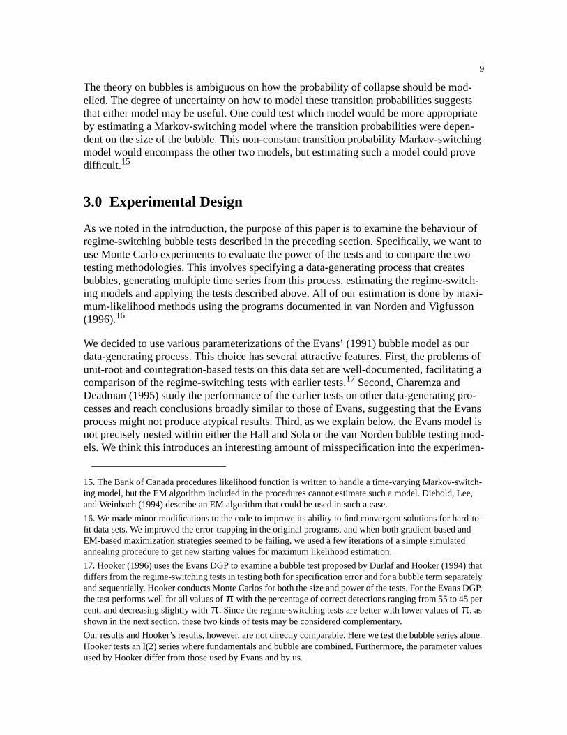
The theory on bubbles is ambiguous on how the probability of collapse should be mod-elled. The degree of uncertainty on how to model these transition probabilities suggeststhat either model may be useful. One could test which model would be more appropriateby estimating a Markov-switching model where the transition probabilities were depen-dent on the size of the bubble. This non-constant transition probability Markov-switchingmodel would encompass the other two models, but estimating such a model could provedifficult.15

3.0 Experimental Design

As we noted in the introduction, the purpose of this paper is to examine the behaviour ofregime-switching bubble tests described in the preceding section. Specifically, we want touse Monte Carlo experiments to evaluate the power of the tests and to compare the twotesting methodologies. This involves specifying a data-generating process that createsbubbles, generating multiple time series from this process, estimating the regime-switch-ing models and applying the tests described above. All of our estimation is done by maxi-mum-likelihood methods using the programs documented in van Norden and Vigfusson(1996).16

We decided to use various parameterizations of the Evans’ (1991) bubble model as ourdata-generating process. This choice has several attractive features. First, the problems ofunit-root and cointegration-based tests on this data set are well-documented, facilitating acomparison of the regime-switching tests with earlier tests.17 Second, Charemza andDeadman (1995) study the performance of the earlier tests on other data-generating pro-cesses and reach conclusions broadly similar to those of Evans, suggesting that the Evansprocess might not produce atypical results. Third, as we explain below, the Evans model isnot precisely nested within either the Hall and Sola or the van Norden bubble testing mod-els. We think this introduces an interesting amount of misspecification into the experimen-

15. The Bank of Canada procedures likelihood function is written to handle a time-varying Markov-switch-ing model, but the EM algorithm included in the procedures cannot estimate such a model. Diebold, Lee,and Weinbach (1994) describe an EM algorithm that could be used in such a case.

16. We made minor modifications to the code to improve its ability to find convergent solutions for hard-to-fit data sets. We improved the error-trapping in the original programs, and when both gradient-based andEM-based maximization strategies seemed to be failing, we used a few iterations of a simple simulatedannealing procedure to get new starting values for maximum likelihood estimation.

17. Hooker (1996) uses the Evans DGP to examine a bubble test proposed by Durlaf and Hooker (1994) thatdiffers from the regime-switching tests in testing both for specification error and for a bubble term separatelyand sequentially. Hooker conducts Monte Carlos for both the size and power of the tests. For the Evans DGP,the test performs well for all values of with the percentage of correct detections ranging from 55 to 45 percent, and decreasing slightly with . Since the regime-switching tests are better with lower values of , asshown in the next section, these two kinds of tests may be considered complementary.

Our results and Hooker’s results, however, are not directly comparable. Here we test the bubble series alone.Hooker tests an I(2) series where fundamentals and bubble are combined. Furthermore, the parameter valuesused by Hooker differ from those used by Evans and by us.

ππ π

10

tal design and may give a better indication of how the tests are likely to perform whenconfronted with real data that may not nest perfectly within either model. We also felt thatit offered a neutral “middle ground” on which to compare the performance of the twotests.

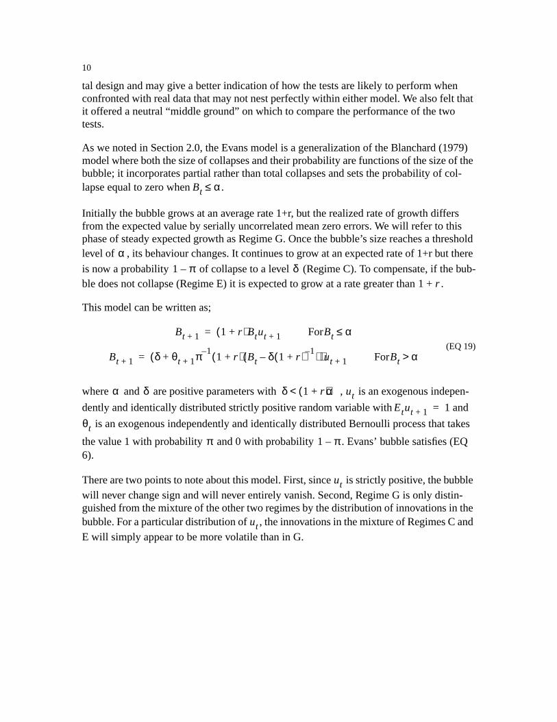
As we noted in Section 2.0, the Evans model is a generalization of the Blanchard (1979)model where both the size of collapses and their probability are functions of the size of thebubble; it incorporates partial rather than total collapses and sets the probability of col-lapse equal to zero when .

Initially the bubble grows at an average rate 1+r, but the realized rate of growth differsfrom the expected value by serially uncorrelated mean zero errors. We will refer to thisphase of steady expected growth as Regime G. Once the bubble’s size reaches a thresholdlevel of , its behaviour changes. It continues to grow at an expected rate of 1+r but there

is now a probability of collapse to a level (Regime C). To compensate, if the bub-ble does not collapse (Regime E) it is expected to grow at a rate greater than .

This model can be written as;

(EQ 19)

where and are positive parameters with , is an exogenous indepen-

dently and identically distributed strictly positive random variable with and

is an exogenous independently and identically distributed Bernoulli process that takes

the value 1 with probability and 0 with probability . Evans’ bubble satisfies (EQ6).

There are two points to note about this model. First, since is strictly positive, the bubblewill never change sign and will never entirely vanish. Second, Regime G is only distin-guished from the mixture of the other two regimes by the distribution of innovations in thebubble. For a particular distribution of , the innovations in the mixture of Regimes C andE will simply appear to be more volatile than in G.

Bt α≤

α1 π– δ

1 r+

Bt 1+ 1 r+( )Btut 1+= ForBt α≤

Bt 1+ δ θt 1+ π 1–+ 1 r+( ) Bt δ 1 r+( )–

1–( )( )ut 1+= ForBt α>

α δ δ 1 r+( )α< utEtut 1+ 1=

θt

π 1 π–

ut

ut

11

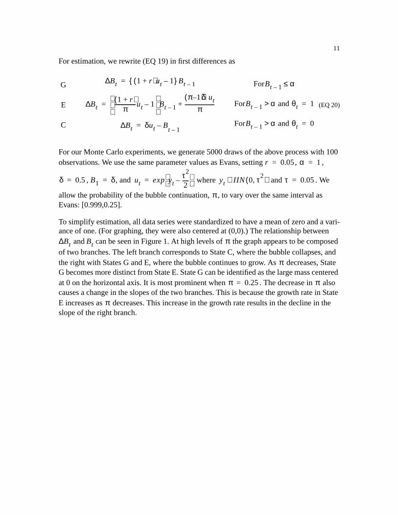
For estimation, we rewrite (EQ 19) in first differences as

(EQ 20)

For our Monte Carlo experiments, we generate 5000 draws of the above process with 100observations. We use the same parameter values as Evans, setting , ,

, , and where and . We

allow the probability of the bubble continuation, , to vary over the same interval asEvans: [0.999,0.25].

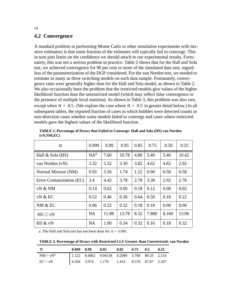
To simplify estimation, all data series were standardized to have a mean of zero and a vari-ance of one. (For graphing, they were also centered at (0,0).) The relationship between

and can be seen in Figure 1. At high levels of the graph appears to be composedof two branches. The left branch corresponds to State C, where the bubble collapses, andthe right with States G and E, where the bubble continues to grow. As decreases, StateG becomes more distinct from State E. State G can be identified as the large mass centeredat 0 on the horizontal axis. It is most prominent when . The decrease in alsocauses a change in the slopes of the two branches. This is because the growth rate in StateE increases as decreases. This increase in the growth rate results in the decline in theslope of the right branch.

G

E

C

Bt∆ 1 r+( )ut 1–{ }Bt 1–=

Bt∆ 1 r+( )π----------------ut 1–

Bt 1–

π 1–( )δut

π-----------------------+=

Bt∆ δut B–t 1–

=

ForBt 1– α≤

ForBt 1– α andθt> 1=

ForBt 1– α andθt> 0=

r 0.05= α 1=

δ 0.5= B1 δ= ut exp ytτ2

2-----–

= yt IIN 0 τ2,( )∼ τ 0.05=

π

Bt∆ Bt π

π

π 0.25= π

π

12

FIGURE 1.

π 0.99= π 0.95=

π 0.85= π 0.75=

π 0.50= π 0.25=

13

4.0 Monte Carlo Results

4.1 Overview of Results

The two regime-switching tests frequently detect bubbles that the unit-root tests incor-rectly reject. When comparing regime-switching with unit-root tests, one must rememberthat the nulls of the two kinds of tests are opposite. One might think that because criticalvalues are chosen to minimize false rejections of the null that the unit-root tests shoulddetect bubbles more often since their null hypothesis is that a bubble exists. As seen inTable 1, this is clearly not the case.

The relationship between the value of and the ability to detect bubbles varies among the

different tests. For values of less than 0.99, the Bhargava (1986) and unit-root

tests frequently and incorrectly reject the null of a bubble in favor of a stationary stablealternative.18 The van Norden test does best when equals 0.75 and does a poorer job forother values. The Hall and Sola test detects more bubbles than van Norden according tothe t-tests for all values of except when equals 0.75.

The following sections give more details on our results. The next section discusses the dif-ficulties experienced in trying to get the maximum-likelihood estimation methods to con-vergence. Following sections discuss each test individually. We then look at the addedinformation each test provides, followed by conclusions.

18. The greatest difference between a percentage that we report and Evans is less than 5 per cent.

TABLE 1. Summary Table: Ability of Tests to Detect Bubbles

Test 0.999 0.99 0.95 0.85 0.75 0.50 0.25

Bhargava N1 rejection in favor ofexplosive alternative

78.5 32.5 0 0 0 0 0

rejection in favor ofstable alternative

0 1 65.5 94.6 98 100 100

Bhargava N2 rejection in favor ofexplosive alternative

95 58 15 4.5 2 1 0

rejection in favor ofstable alternative

0 1 18.5 90 94.5 97 97

van Norden correct signs 8 89.5 82.5 96 99 89.5 95

t-test 1 5 16 48.5 77 28.5 3

Hall & Sola correct signs 39.5 67.5 78.5 83.5 83.5 71

t-test 25 50 64 64 58 35

ππ N1 N2

π

π π

14

4.2 Convergence

A standard problem in performing Monte Carlo or other simulation experiments with iter-ative estimators is that some fraction of the estimates will typically fail to converge. Thisin turn puts limits on the confidence we should attach to our experimental results. Fortu-nately, this was not a serious problem in practice. Table 2 shows that for the Hall and Solatest, we achieved convergence for 90 per cent or more of the simulated data sets, regard-less of the parameterization of the DGP considered. For the van Norden test, we needed toestimate as many as three switching models on each data sample. Fortunately, conver-gence rates were generally higher than for the Hall and Sola model, as shown in Table 2.We also occasionally have the problem that the restricted models give values of the higherlikelihood function than the unrestricted model (which may reflect false convergence orthe presence of multiple local maxima). As shown in Table 3, this problem was also rare,except when . (We explore the case where in greater detail below.) In allsubsequent tables, the reported fraction of cases in which bubbles were detected counts asnon-detection cases whether some models failed to converge and cases where restrictedmodels gave the highest values of the likelihood function.

a. The Hall and Sola test has not been done for .

TABLE 2. Percentage of Draws that Failed to Converge: Hall and Sola (HS) van Norden(vN,NM,EC)

0.999 0.99 0.95 0.85 0.75 0.50 0.25

Hall & Sola (HS) NAa 7.60 10.78 4.80 3.40 3.46 10.42

van Norden (vN) 3.32 5.32 3.30 3.82 4.62 4.82 2.92

Normal Mixture (NM) 0.92 3.56 1.74 1.22 0.90 0.58 0.58

Error Contamination (EC) 3.4 4.42 3.78 2.78 3.38 2.92 2.76

vN & NM 0.14 0.62 0.06 0.18 0.12 0.08 0.02

vN & EC 0.52 0.46 0.36 0.64 0.50 0.18 0.22

NM & EC 0.06 0.22 0.32 0.18 0.18 0.08 0.06

NA 11.98 13.78 8.32 7.880 8.160 13.06

HS & vN NA 1.00 0.34 0.32 0.16 0.18 0.32

TABLE 3. Percentage of Draws with Restricted LLF Greater than Unrestricted: van Norden

0.999 0.99 0.95 0.85 0.75 0.5 0.25

NM > vNa 1.122 0.4862 0.04138 0.2080 5.789 88.33 2.514

EC > vN 6.594 3.974 1.179 1.414 8.578 87.87 2.267

π 0.5= π 0.5=

π

π 0.999=

HS vN∪

π

15

4.3 Hall and Sola Test

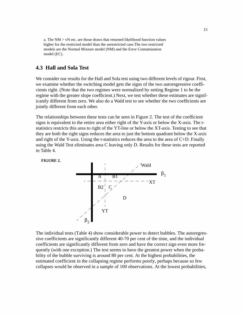
We consider our results for the Hall and Sola test using two different levels of rigour. First,we examine whether the switching model gets the signs of the two autoregressive coeffi-cients right. (Note that the two regimes were normalized by setting Regime 1 to be theregime with the greater slope coefficient.) Next, we test whether these estimates are signif-icantly different from zero. We also do a Wald test to see whether the two coefficients arejointly different from each other.

The relationships between these tests can be seen in Figure 2. The test of the coefficientsigns is equivalent to the entire area either right of the Y-axis or below the X-axis. The t-statistics restricts this area to right of the YT-line or below the XT-axis. Testing to see thatthey are both the right signs reduces the area to just the bottom quadrant below the X-axisand right of the Y-axis. Using the t-statistics reduces the area to the area of C+D. Finallyusing the Wald Test eliminates area C leaving only D. Results for these tests are reportedin Table 4.

FIGURE 2.

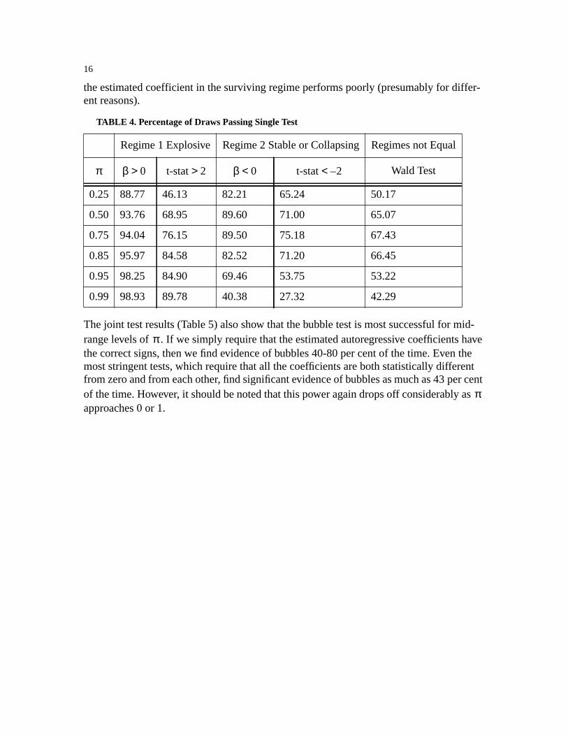
The individual tests (Table 4) show considerable power to detect bubbles. The autoregres-sive coefficients are significantly different 40-70 per cent of the time, and the individualcoefficients are significantly different from zero and have the correct sign even more fre-quently (with one exception.) The test seems to have the greatest power when the proba-bility of the bubble surviving is around 80 per cent. At the highest probabilities, theestimated coefficient in the collapsing regime performs poorly, perhaps because so fewcollapses would be observed in a sample of 100 observations. At the lowest probabilities,

a. The NM > vN etc. are those draws that returned likelihood function valueshigher for the restricted model than the unrestricted case.The two restrictedmodels are the Normal Mixture model (NM) and the Error Contaminationmodel (EC).

A

C

B1

B2

D

β1

β2

YT

XT

Wald

16

the estimated coefficient in the surviving regime performs poorly (presumably for differ-ent reasons).

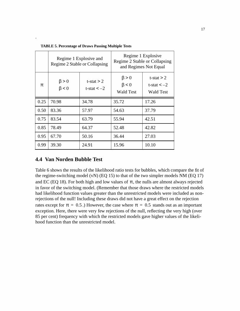
The joint test results (Table 5) also show that the bubble test is most successful for mid-range levels of . If we simply require that the estimated autoregressive coefficients havethe correct signs, then we find evidence of bubbles 40-80 per cent of the time. Even themost stringent tests, which require that all the coefficients are both statistically differentfrom zero and from each other, find significant evidence of bubbles as much as 43 per centof the time. However, it should be noted that this power again drops off considerably asapproaches 0 or 1.

TABLE 4. Percentage of Draws Passing Single Test

Regime 1 Explosive Regime 2 Stable or Collapsing Regimes not Equal

Wald Test

0.25 88.77 46.13 82.21 65.24 50.17

0.50 93.76 68.95 89.60 71.00 65.07

0.75 94.04 76.15 89.50 75.18 67.43

0.85 95.97 84.58 82.52 71.20 66.45

0.95 98.25 84.90 69.46 53.75 53.22

0.99 98.93 89.78 40.38 27.32 42.29

π β 0> t-stat 2> β 0< t-stat 2–<

π

π

17

.

4.4 Van Norden Bubble Test

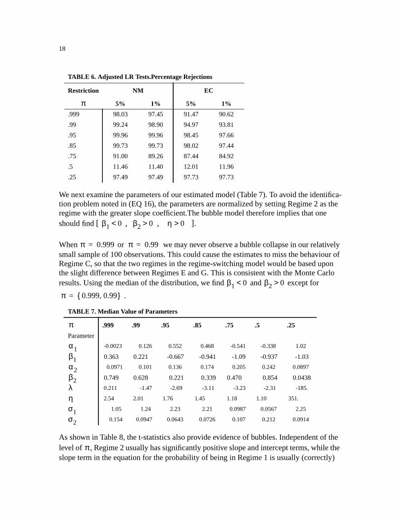
Table 6 shows the results of the likelihood ratio tests for bubbles, which compare the fit ofthe regime-switching model (vN) (EQ 15) to that of the two simpler models NM (EQ 17)and EC (EQ 18). For both high and low values of , the nulls are almost always rejectedin favor of the switching model. (Remember that those draws where the restricted modelshad likelihood function values greater than the unrestricted models were included as non-rejections of the null! Including these draws did not have a great effect on the rejectionrates except for .) However, the case where stands out as an importantexception. Here, there were very few rejections of the null, reflecting the very high (over85 per cent) frequency with which the restricted models gave higher values of the likeli-hood function than the unrestricted model.

TABLE 5. Percentage of Draws Passing Multiple Tests

Regime 1 Explosive andRegime 2 Stable or Collapsing

Regime 1 ExplosiveRegime 2 Stable or Collapsing

and Regimes Not Equal

0.25 70.98 34.78 35.72 17.26

0.50 83.36 57.97 54.63 37.79

0.75 83.54 63.79 55.94 42.51

0.85 78.49 64.37 52.48 42.82

0.95 67.70 50.16 36.44 27.03

0.99 39.30 24.91 15.96 10.10

πβ 0>β 0<

t-stat 2>t-stat 2–<

β 0>β 0<

Wald Test

t-stat 2>t-stat 2–<Wald Test

π

π 0.5= π 0.5=

18

We next examine the parameters of our estimated model (Table 7). To avoid the identifica-tion problem noted in (EQ 16), the parameters are normalized by setting Regime 2 as theregime with the greater slope coefficient.The bubble model therefore implies that oneshould find[ , , ].

When or we may never observe a bubble collapse in our relativelysmall sample of 100 observations. This could cause the estimates to miss the behaviour ofRegime C, so that the two regimes in the regime-switching model would be based uponthe slight difference between Regimes E and G. This is consistent with the Monte Carloresults. Using the median of the distribution, we find and except for

.

As shown in Table 8, the t-statistics also provide evidence of bubbles. Independent of thelevel of , Regime 2 usually has significantly positive slope and intercept terms, while theslope term in the equation for the probability of being in Regime 1 is usually (correctly)

TABLE 6. Adjusted LR Tests.Percentage Rejections

Restriction NM EC

5% 1% 5% 1%

.999 98.03 97.45 91.47 90.62

.99 99.24 98.90 94.97 93.81

.95 99.96 99.96 98.45 97.66

.85 99.73 99.73 98.02 97.44

.75 91.00 89.26 87.44 84.92

.5 11.46 11.40 12.01 11.96

.25 97.49 97.49 97.73 97.73

TABLE 7. Median Value of Parameters

.999 .99 .95 .85 .75 .5 .25

Parameter

-0.0023 0.126 0.552 0.468 -0.541 -0.338 1.02

0.363 0.221 -0.667 -0.941 -1.09 -0.937 -1.03

0.0971 0.101 0.136 0.174 0.205 0.242 0.0897

0.749 0.628 0.221 0.339 0.470 0.854 0.0438

0.211 -1.47 -2.69 -3.11 -3.23 -2.31 -185.

2.54 2.01 1.76 1.45 1.18 1.10 351.

1.05 1.24 2.23 2.21 0.0987 0.0567 2.25

0.154 0.0947 0.0643 0.0726 0.107 0.212 0.0914

π

β1 0< β2 0> η 0>

π 0.999= π 0.99=

β1 0< β2 0>

π 0.999 0.99,{ }=

π

α1β1α2β2λησ1σ2

π

19

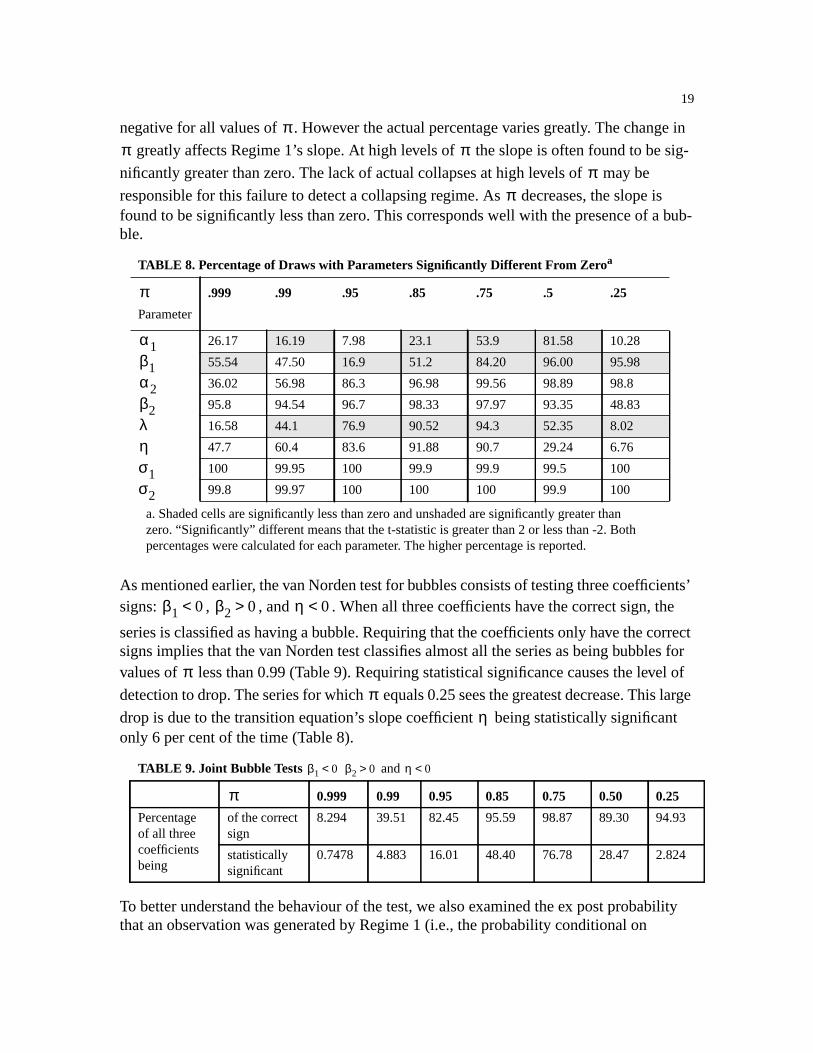
negative for all values of . However the actual percentage varies greatly. The change in

greatly affects Regime 1’s slope. At high levels of the slope is often found to be sig-

nificantly greater than zero. The lack of actual collapses at high levels of may be

responsible for this failure to detect a collapsing regime. As decreases, the slope isfound to be significantly less than zero. This corresponds well with the presence of a bub-ble.

As mentioned earlier, the van Norden test for bubbles consists of testing three coefficients’signs: , , and . When all three coefficients have the correct sign, the

series is classified as having a bubble. Requiring that the coefficients only have the correctsigns implies that the van Norden test classifies almost all the series as being bubbles forvalues of less than 0.99 (Table 9). Requiring statistical significance causes the level of

detection to drop. The series for which equals 0.25 sees the greatest decrease. This large

drop is due to the transition equation’s slope coefficient being statistically significantonly 6 per cent of the time (Table 8).

To better understand the behaviour of the test, we also examined the ex post probabilitythat an observation was generated by Regime 1 (i.e., the probability conditional on

a. Shaded cells are significantly less than zero and unshaded are significantly greater thanzero. “Significantly” different means that the t-statistic is greater than 2 or less than -2. Bothpercentages were calculated for each parameter. The higher percentage is reported.

TABLE 8. Percentage of Draws with Parameters Significantly Different From Zeroa

.999 .99 .95 .85 .75 .5 .25

Parameter

26.17 16.19 7.98 23.1 53.9 81.58 10.28

55.54 47.50 16.9 51.2 84.20 96.00 95.98

36.02 56.98 86.3 96.98 99.56 98.89 98.8

95.8 94.54 96.7 98.33 97.97 93.35 48.83

16.58 44.1 76.9 90.52 94.3 52.35 8.02

47.7 60.4 83.6 91.88 90.7 29.24 6.76

100 99.95 100 99.9 99.9 99.5 100

99.8 99.97 100 100 100 99.9 100

TABLE 9. Joint Bubble Tests and

0.999 0.99 0.95 0.85 0.75 0.50 0.25

Percentageof all threecoefficientsbeing

of the correctsign

8.294 39.51 82.45 95.59 98.87 89.30 94.93

statisticallysignificant

0.7478 4.883 16.01 48.40 76.78 28.47 2.824

ππ π

ππ

π

α1β1α2β2λησ1σ2

β1 0< β2 0> η 0<

ππ

η

β1 0< β2 0> η 0<

π

20

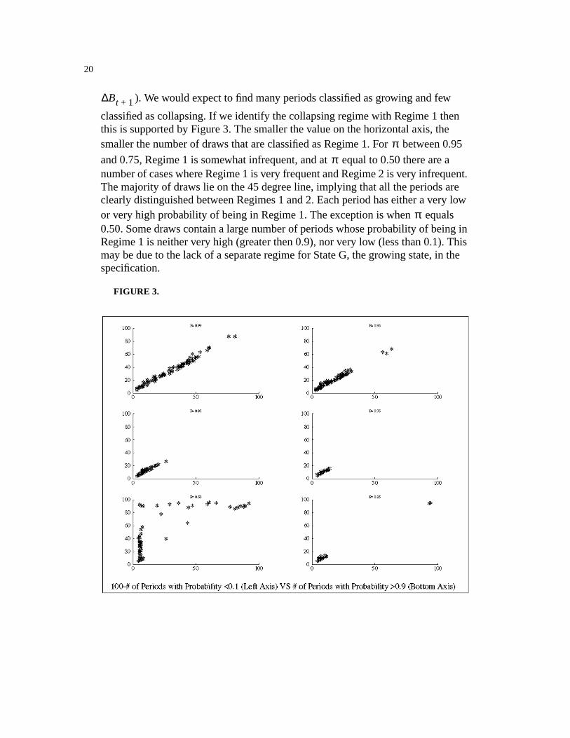
). We would expect to find many periods classified as growing and few

classified as collapsing. If we identify the collapsing regime with Regime 1 thenthis is supported by Figure 3. The smaller the value on the horizontal axis, thesmaller the number of draws that are classified as Regime 1. For between 0.95

and 0.75, Regime 1 is somewhat infrequent, and at equal to 0.50 there are anumber of cases where Regime 1 is very frequent and Regime 2 is very infrequent.The majority of draws lie on the 45 degree line, implying that all the periods areclearly distinguished between Regimes 1 and 2. Each period has either a very lowor very high probability of being in Regime 1. The exception is when equals0.50. Some draws contain a large number of periods whose probability of being inRegime 1 is neither very high (greater then 0.9), nor very low (less than 0.1). Thismay be due to the lack of a separate regime for State G, the growing state, in thespecification.

FIGURE 3.

Bt 1+∆

ππ

π

21

4.5 Comparing van Norden and Hall and Sola

Having examined the individual performances of the two tests, we now use the two teststogether. First, we examine how often the tests agree that a bubble is present. Second, weexamine how often one test confirms the presence of a bubble already detected by theother.

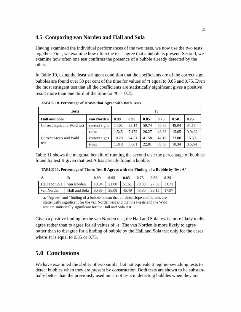
In Table 10, using the least stringent condition that the coefficients are of the correct sign,bubbles are found over 50 per cent of the time for values of equal to 0.85 and 0.75. Eventhe most stringent test that all the coefficients are statistically significant gives a positiveresult more than one third of the time for .

Table 11 shows the marginal benefit of running the second test: the percentage of bubblesfound by test B given that test A has already found a bubble.

Given a positive finding by the van Norden test, the Hall and Sola test is more likely to dis-agree rather than to agree for all values of . The van Norden is more likely to agreerather than to disagree for a finding of bubble by the Hall and Sola test only for the caseswhere is equal to 0.85 or 0.75.

5.0 Conclusions

We have examined the ability of two similar but not equivalent regime-switching tests todetect bubbles when they are present by construction. Both tests are shown to be substan-tially better than the previously used unit-root tests in detecting bubbles when they are

a. “Agrees” and “finding of a bubble” mean that all three slope coefficients arestatistically significant for the van Norden test and that the t-tests and the Waldtest are statistically significant for the Hall and Sola test.

TABLE 10. Percentage of Draws that Agree with Both Tests

Tests

Hall and Sola van Norden 0.99 0.95 0.85 0.75 0.50 0.25

Correct signs and Wald test correct signs 14.02 33.14 50.74 55.38 49.04 34.18

t-test 1.545 7.172 26.27 43.36 15.05 0.9432

Correct t-tests and Waldtest

correct signs 10.20 24.51 41.58 42.16 33.80 16.59

t-test 1.318 5.661 22.01 33.56 10.34 0.5291

TABLE 11. Percentage of Times Test B Agrees with the Finding of a Bubble by Test Aa

A B 0.99 0.95 0.85 0.75 0.50 0.25

Hall and Sola van Norden 10.94 21.00 51.61 79.00 27.36 3.071

van Norden Hall and Sola 30.85 36.08 45.49 43.80 36.15 17.97

π

π 0.75=

π

π

π

22

present by construction. In particular, Evans (1991) showed that unit-root tests may inad-vertently suggest the absence of bubbles when several regime switches are encountered inthe sample; this seems to be when regime-switching methods have the most power todetect bubbles.

When used with similar dependent variables, the two regime-switching tests differ in threeways. First, the Hall and Sola test allows for more complicated dynamics within regimesby including lagged changes in the asset price. Second, the probability of being in a cer-tain regime for Hall and Sola depends on last period’s regime, while the same probabilityfor van Norden’s test depends on last period’s value of the bubble. Third, to the extent thatthere are variations in the fundamental value of the asset, the tests use different explana-tory variables; Hall and Sola use the asset’s price while van Norden uses the differencebetween this price and the fundamental prices. These differences in structure result in thetwo tests having different abilities to detect bubbles. In this paper, we focussed on the sec-ond of these three differences, and found that the van Norden test tended to have morepower than the Hall and Sola test for certain values of the probability of the bubble con-tinuing to grow , but that the power of the Hall and Sola test was less sensitive to the

value of .

Even though the tests are different, we currently cannot say that one test is superior to theother. The van Norden test did have higher rates of convergence, but convergence is likelyto be more of an issue for a Monte Carlo study than for applied research. To establishwhich test, if either, is better would require more work.The power of each test when thebubble term is measured with serially correlated errors will be an important topic to exam-ine. Serially correlated errors could likely be the case when applied to actual data. The sizeof the tests will also need to be examined. The ability of the regime-switching tests todetect bubbles when they are present will be of little use to the applied researcher if thetests also find many false positives.

ππ

23

6.0 Bibliography

Allen, Franklin and Gary Gorton. 1991.“ Rational Finite Bubbles.” Working PaperNo. 3707. National Bureau for Economic Research, Cambridge.

Bhargava, Alok. 1986. “On the Theory of Testing for Unit Roots in Observed TimeSeries.” Review of Economic Studies 53:369-84.

Blanchard, Oliver J. 1979. “Speculative Bubbles, Crashes, and RationalExpectations.”Economic Letters 3(4):387-9

Buiter, Willem H. and Paolo A. Pesenti. 1990. “Rational Speculative Bubbles in anExchange Rate Target Zone.” Discussion Paper No. 479. Centre forEconomic Policy Research.

Bulow, Jeremy and Paul Klemperer. 1994) “Rational Frenzies and Crashes.”Journalof Political Economy 102(1):1-23.

Charemza, Wojciech W. and Derek F. Deadman. 1995. “Speculative bubbles withstochastic explosive roots: the failure of unit root testing.”Journal ofEmpirical Finance 2:153-163.

De Long, J. B., Andrei Shleifer, Lawrence Summers and R. Waldman. 1990. “NoiseTrader Risk in Financial Markets.”Journal of Political Economy 98:703-38.

Diebold, Francis X. Joon Haeng Lee and Gretchen C. Weinbach. 1994. “RegimeSwitching with Time Varying Transition Probabilities.” In C. Hargreaves,Nonstationary Time Series Analysis and Cointegration.Oxford, OxfordUniversity Press.

Diba, Behzad T., and Herschel I. Grossman. 1987. “On the Inception of RationalBubbles.”Quarterly Journal of Economics 102:697-700.

Diba, Behzad T., and Herschel I. Grossman. 1988. “Explosive Rational Bubbles inStock Prices?”American Economic Review 78:520-30.

Durlaf, Stephen. and Mark A. Hooker. 1994. “Misspecificaton versus Bubbles in theCagan Hyperinflation Model.” In C. Hargreaves,Nonstationary Time SeriesAnalysis and Cointegration.Oxford, Oxford University Press.

Evans, George W. 1991. “Pitfalls in Testing for Explosive Bubbles in Asset Prices.”American Economic Review 4:922-30

Evans, Martin D. D. and Karen Lewis. 1995. “Do long-term swings in the dollaraffect estimates of the risk premia?”Review of Financial Studies 8(3):709-42.

24

Flood, Robert P. and Robert J. Hodrick. 1990. “On Testing for Speculative Bubbles.”Journal of Economic Perspectives 4(2):85-102.

Froot, K.A. and M. Obstfeld. 1991. “Intrinsic Bubbles: the Case of Stock Prices.”The American Economic Review81(5):1189-214.

Funke, Michael, Stephen Hall and Martin Sola. 1994. “Rational Bubbles DuringPoland’s Hyperinflation: Implications and Empirical Evidence.”EuropeanEconomic Review 38:1257-76.

Gilles, C. and S.F. LeRoy. 1992. “Bubbles and Charges.”International EconomicReview 33(2):323-339.

Hall, Stephen and Martin Sola. 1993.Testing for Collapsing Bubbles; AnEndogenous Switching ADF Test. discussion paper 15-93, London BusinessSchool.

Hamilton, James and Charles Whiteman. 1985. “The Observable Implications ofSelf-Fulfilling Expectations.”Journal of Monetary Economics 16:353-74.

Hamilton, James D. 1989. “A New Approach to the Economic Analysis ofNonstationary Time Series and the Business Cycle.”Econometrica57(2):357-84

Hamilton, James D. 1994.Time Series Analysis. Princeton: Princeton UniversityPress.

Hooker, Mark A. 1996. “Misspecification versus Bubbles in Hyperinflation Data:Monte Carlo and Interwar European Evidence.” Manuscript.

Kindleberger, C.P. 1989.Manias, Panics and Crashes: A History of FinancialCrises. New York: Basic Books, revised.

LeRoy, Stephen F. 1989. “Efficient Capital Markets and Martingales.”Journal ofEconomic LiteratureXXVII(4):583-1622.

Obstfeld, M. and K. Rogoff. 1983. “Speculative Hyperinflations in MaximizingModels: Can We Rule Them Out?”Journal of Political Economy 91:675-87.

Obstfeld, M. and K. Rogoff. 1986) “Ruling Out Divergent Speculative Bubbles.”Journal of Monetary Economics 17(3):349-62.

Schaller, Huntley and Simon van Norden. 1994. “Regime Switching in StockMarket Returns.” Mimeo

Shiller, Robert J. 1981. “Do Stock Prices Move Too Much to be Justified bySubsequent Changes in Dividends?”American Economic Review 71:421-36.

25

Tirole, J. 1982. “On the Possibility of Speculation Under Rational Expectations.”Econometrica 50(5):1163-81.

Tirole, J. 1985) “Asset Bubbles and Overlapping Generations.”Econometrica 53:1071-1100.

Van Norden, Simon. 1996. “Regime Switching as a Test for Exchange RateBubbles.”Journal of Applied Econometrics, forthcoming.

Van Norden, S. and H. Schaller. 1993a. “The Predictability of Stock Market Regime:Evidence from the Toronto Stock Exchange.”The Review of Economics andStatistics.

Van Norden, S. and H. Schaller. 1993b. “Speculative Behaviour, Regime-Switching,and Stock Market Fundamentals.” Working Paper No. 93-2, Bank of Canada.

Van Norden, Simon and Robert Vigfusson. 1996. “Regime-Switching Models: AGuide to the Bank of Canada Gauss Procedures.” Working Paper 96-3, Bankof Canada.

Weil, P. 1990. “On the Possibility of Price Decreasing Bubbles.”Econometrica58(6):1467-74.

West, Kenneth D. 1987. “A Specification Test for Speculative Bubbles.”QuarterlyJournal of Economics 102:553-80.