Avoiding Communicationin

Linear Algebra

Jim DemmelUC Berkeley

bebop.cs.berkeley.edu

Motivation • Running time of an algorithm is sum of 3 terms:• # flops * time_per_flop• # words moved / bandwidth• # messages * latency

communication

Motivation • Running time of an algorithm is sum of 3 terms:• # flops * time_per_flop• # words moved / bandwidth• # messages * latency

• Exponentially growing gaps between• Time_per_flop << 1/Network BW << Network Latency• Improving 59%/year vs 26%/year vs 15%/year

• Time_per_flop << 1/Memory BW << Memory Latency• Improving 59%/year vs 23%/year vs 5.5%/year

communication

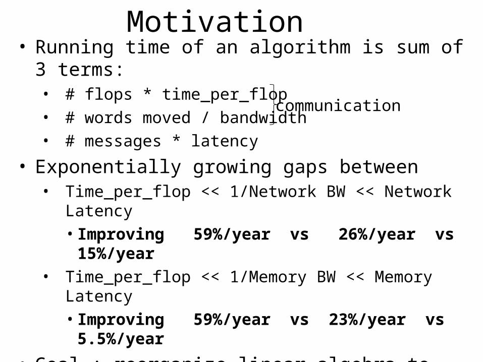
Motivation • Running time of an algorithm is sum of 3 terms:• # flops * time_per_flop• # words moved / bandwidth• # messages * latency

• Exponentially growing gaps between• Time_per_flop << 1/Network BW << Network Latency• Improving 59%/year vs 26%/year vs 15%/year

• Time_per_flop << 1/Memory BW << Memory Latency• Improving 59%/year vs 23%/year vs 5.5%/year

• Goal : reorganize linear algebra to avoid communication• Not just hiding communication (speedup 2x ) • Arbitrary speedups possible

communication

Outline

• Motivation• Avoiding Communication in Dense Linear

Algebra• Avoiding Communication in Sparse Linear

Algebra

Outline

• Motivation• Avoiding Communication in Dense Linear

Algebra• Avoiding Communication in Sparse Linear

Algebra• A poem in memory of Gene Golub (separate file)

Collaborators (so far)• UC Berkeley– Kathy Yelick, Ming Gu– Mark Hoemmen, Marghoob Mohiyuddin, Kaushik Datta,

George Petropoulos, Sam Williams, BeBOp group– Lenny Oliker, John Shalf

• CU Denver – Julien Langou

• INRIA– Laura Grigori, Hua Xiang

• Much related work– Complete references in technical reports

Why all our problems are solved for dense linear algebra– in theory

• (Talk by Ioana Dumitriu on Monday)• Thm (D., Dumitriu, Holtz, Kleinberg) (Numer.Math. 2007)

– Given any matmul running in O(n) ops for some >2, it can be made stable and still run in O(n+) ops, for any >0.• Current record: 2.38

• Thm (D., Dumitriu, Holtz) (Numer. Math. 2008)– Given any stable matmul running in O(n+) ops, it is possible

to do backward stable dense linear algebra in O(n+) ops:• GEPP, QR • rank revealing QR (randomized)• (Generalized) Schur decomposition, SVD (randomized)

• Also reduces communication to O(n+) • But constants?

8

Summary (1) – Avoiding Communication in Dense Linear Algebra

• QR or LU decomposition of m x n matrix, m >> n– Parallel implementation

• Conventional: O( n log p ) messages• “New”: O( log p ) messages - optimal

– Serial implementation with fast memory of size F• Conventional: O( mn/F ) moves of data from slow to fast memory

– mn/F = how many times larger matrix is than fast memory• “New”: O(1) moves of data - optimal

– Lots of speed up possible (measured and modeled) • Price: some redundant computation, stability?

• Extends to square case, with optimality results• Extends to other architectures (eg multicore)• (Talk by Julien Langou Monday, on QR)

Minimizing Comm. in Parallel QR

W = W0

W1

W2

W3

R00

R10

R20

R30

R01

R11

R02

• QR decomposition of m x n matrix W, m >> n• TSQR = “Tall Skinny QR”• P processors, block row layout

• Usual Parallel Algorithm• Compute Householder vector for each column• Number of messages n log P

• Communication Avoiding Algorithm• Reduction operation, with QR as operator• Number of messages log P

TSQR in more detail

30

20

10

00

30

20

10

00

3

2

1

0

.

R

R

R

R

Q

Q

Q

Q

W

W

W

W

W

11

01

11

01

30

20

10

00

.R

R

Q

Q

R

R

R

R

020211

01 RQR

R

Q is represented implicitly as a product (tree of factors)

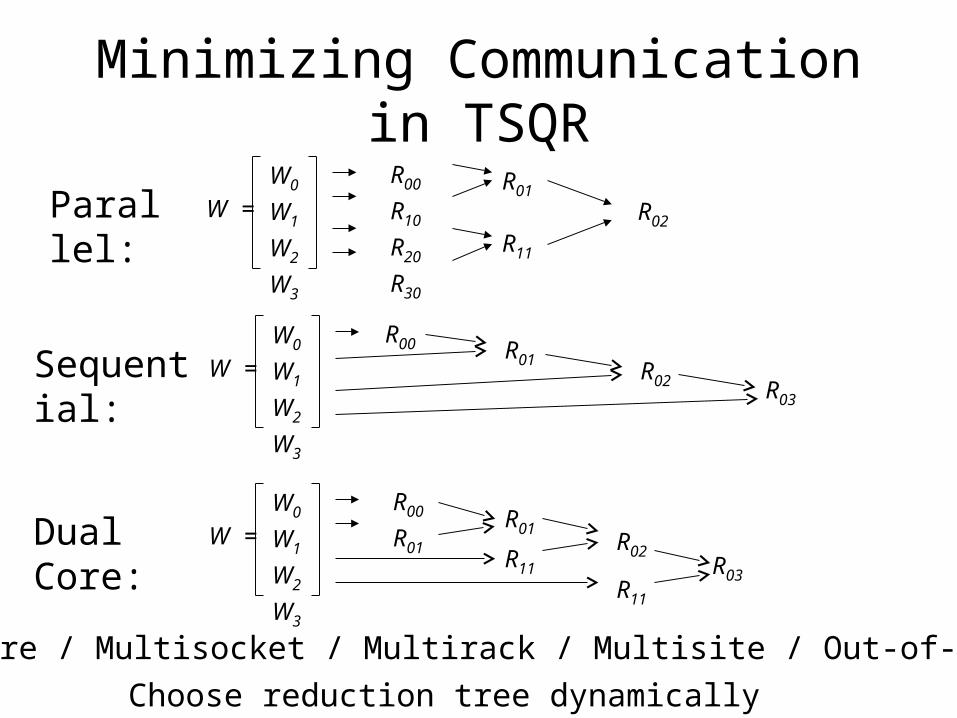
Minimizing Communication in TSQR

W = W0

W1

W2

W3

R00

R10

R20

R30

R01

R11

R02Parallel:

W = W0

W1

W2

W3

R01 R02

R00

R03

Sequential:

W = W0

W1

W2

W3

R00

R01

R01

R11

R02

R11

R03

Dual Core:

Choose reduction tree dynamicallyMulticore / Multisocket / Multirack / Multisite / Out-of-core: ?

Performance of TSQR vs Sca/LAPACK

• Parallel– Pentium III cluster, Dolphin Interconnect, MPICH• Up to 6.7x speedup (16 procs, 100K x 200)

– BlueGene/L• Up to 4x speedup (32 procs, 1M x 50)

– Both use Elmroth-Gustavson locally – enabled by TSQR• Sequential – OOC on PowerPC laptop• As little as 2x slowdown vs (predicted) infinite DRAM

• See UC Berkeley EECS Tech Report 2008-74

QR for General Matrices• CAQR – Communication Avoiding QR for general A– Use TSQR for panel factorizations– Apply to rest of matrix

• Cost of CAQR vs ScaLAPACK’s PDGEQRF– n x n matrix on P1/2 x P1/2 processor grid, block size b– Flops: (4/3)n3/P + (3/4)n2b log P/P1/2 vs (4/3)n3/P – Bandwidth: (3/4)n2 log P/P1/2 vs same– Latency: 2.5 n log P / b vs 1.5 n log P

• Close to optimal (modulo log P factors)– Assume: O(n2/P) memory/processor, O(n3) algorithm, – Choose b near n / P1/2 (its upper bound)– Bandwidth lower bound: (n2 /P1/2) – just log(P) smaller– Latency lower bound: (P1/2) – just polylog(P) smaller– Extension of Irony/Toledo/Tishkin (2004)

• Implementation – Julien’s summer project

Modeled Speedups of CAQR vs ScaLAPACK

Petascale up to 22.9x

IBM Power 5 up to 9.7x

“Grid” up to 11x

Petascale machine with 8192 procs, each at 500 GFlops/s, a bandwidth of 4 GB/s../102,10,102 9512 wordsss

TSLU: LU factorization of a tall skinny matrix

30

20

10

00

30

20

10

00

30

20

10

00

3

2

1

0

.

0

U

U

U

U

L

L

L

L

W

W

W

W

W

11

01

11

01

11

01

30

20

10

00

..

1

U

U

L

L

U

U

U

U

020202

11

01

2

ULU

U

First try the obvious generalization of TSQR:

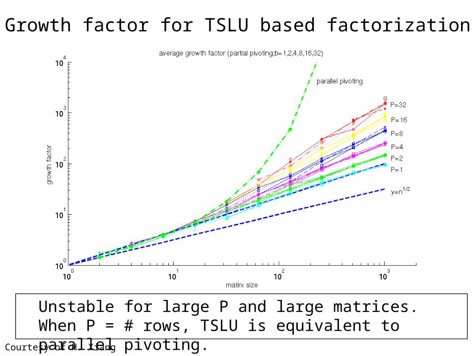
Growth factor for TSLU based factorization

Unstable for large P and large matrices.When P = # rows, TSLU is equivalent to parallel pivoting.

Courtesy of H. Xiang

Making TSLU Stable• At each node in tree, TSLU selects b pivot rows from 2b

candidates from its 2 child nodes• At each node, do LU on 2b original rows selected by child

nodes, not U factors from child nodes• When TSLU done, permute b selected rows to top of original

matrix, redo b steps of LU without pivoting• CALU – Communication Avoiding LU for general A

– Use TSLU for panel factorizations– Apply to rest of matrix– Cost: redundant panel factorizations

• Benefit: – Stable in practice, but not same pivot choice as GEPP– b times fewer messages overall - faster

Growth factor for better CALU approach

Like threshold pivoting with worst case threshold = .33 , so |L| <= 3Testing shows about same residual as GEPP

Performance vs ScaLAPACK• TSLU– IBM Power 5 • Up to 4.37x faster (16 procs, 1M x 150)

– Cray XT4• Up to 5.52x faster (8 procs, 1M x 150)

• CALU– IBM Power 5• Up to 2.29x faster (64 procs, 1000 x 1000)

– Cray XT4• Up to 1.81x faster (64 procs, 1000 x 1000)

• Optimality analysis analogous to QR• See INRIA Tech Report 6523 (2008)

Petascale machine with 8192 procs, each at 500 GFlops/s, a bandwidth of 4 GB/s.

Speedup prediction for a Petascale machine - up to 81x faster

./102,10,102 9512 wordsss

P = 8192

Summary (2) – Avoiding Communication in Sparse Linear Algebra

• Take k steps of Krylov subspace method– GMRES, CG, Lanczos, Arnoldi– Assume matrix “well-partitioned,” with modest surface-

to-volume ratio– Parallel implementation

• Conventional: O(k log p) messages• “New”: O(log p) messages - optimal

– Serial implementation• Conventional: O(k) moves of data from slow to fast memory• “New”: O(1) moves of data – optimal

• Can incorporate some preconditioners– Hierarchical, semiseparable matrices …

• Lots of speed up possible (modeled and measured)– Price: some redundant computation

x

Ax

A2x

A3x

A4x

A5x

A6x

A7x

A8x

Locally Dependent Entries for [x,Ax], A tridiagonal, 2 processors

Can be computed without communication

Proc 1 Proc 2

x

Ax

A2x

A3x

A4x

A5x

A6x

A7x

A8x

Can be computed without communication

Proc 1 Proc 2

Locally Dependent Entries for [x,Ax,A2x], A tridiagonal, 2 processors

x

Ax

A2x

A3x

A4x

A5x

A6x

A7x

A8x

Can be computed without communication

Proc 1 Proc 2

Locally Dependent Entries for [x,Ax,…,A3x], A tridiagonal, 2 processors

x

Ax

A2x

A3x

A4x

A5x

A6x

A7x

A8x

Can be computed without communication

Proc 1 Proc 2

Locally Dependent Entries for [x,Ax,…,A4x], A tridiagonal, 2 processors

x

Ax

A2x

A3x

A4x

A5x

A6x

A7x

A8x

Locally Dependent Entries for [x,Ax,…,A8x], A tridiagonal, 2 processors

Can be computed without communicationk=8 fold reuse of A

Proc 1 Proc 2

Remotely Dependent Entries for [x,Ax,…,A8x], A tridiagonal, 2 processors

x

Ax

A2x

A3x

A4x

A5x

A6x

A7x

A8x

One message to get data needed to compute remotely dependent entries, not k=8Minimizes number of messages = latency cost

Price: redundant work “surface/volume ratio”

Proc 1 Proc 2

Fewer Remotely Dependent Entries for [x,Ax,…,A8x], A tridiagonal, 2 processors

x

Ax

A2x

A3x

A4x

A5x

A6x

A7x

A8x

Reduce redundant work by half

Proc 1 Proc 2

Remotely Dependent Entries for [x,Ax,A2x,A3x], A irregular, multiple processors

Sequential [x,Ax,…,A4x], with memory hierarchy

v

One read of matrix from slow memory, not k=4Minimizes words moved = bandwidth cost

No redundant work

Performance Results

• Measured– Sequential/OOC speedup up to 3x

• Modeled – Sequential/multicore speedup up to 2.5x– Parallel/Petascale speedup up to 6.9x – Parallel/Grid speedup up to 22x

• See bebop.cs.berkeley.edu/#pubs

Optimizing Communication Complexity of Sparse Solvers

• Example: GMRES for Ax=b on “2D Mesh”– x lives on n-by-n mesh– Partitioned on p½ -by- p½ grid– A has “5 point stencil” (Laplacian)• (Ax)(i,j) = linear_combination(x(i,j), x(i,j±1), x(i±1,j))

– Ex: 18-by-18 mesh on 3-by-3 grid

Minimizing Communication of GMRES• What is the cost = (#flops, #words, #mess)

of k steps of standard GMRES?

GMRES, ver.1: for i=1 to k w = A * v(i-1) MGS(w, v(0),…,v(i-1)) update v(i), H endfor solve LSQ problem with H n/p½

n/p½

• Cost(A * v) = k * (9n2 /p, 4n / p½ , 4 )• Cost(MGS) = k2/2 * ( 4n2 /p , log p , log p )• Total cost ~ Cost( A * v ) + Cost (MGS)• Can we reduce the latency?

Minimizing Communication of GMRES• Cost(GMRES, ver.1) = Cost(A*v) + Cost(MGS)

• Cost(W) = ( ~ same, ~ same , 8 )• Latency cost independent of k – optimal

• Cost (MGS) unchanged• Can we reduce the latency more?

= ( 9kn2 /p, 4kn / p½ , 4k ) + ( 2k2n2 /p , k2 log p / 2 , k2 log p / 2 )

• How much latency cost from A*v can you avoid? Almost all

GMRES, ver. 2: W = [ v, Av, A2v, … , Akv ] [Q,R] = MGS(W) Build H from R, solve LSQ problem

k = 3

Minimizing Communication of GMRES• Cost(GMRES, ver. 2) = Cost(W) + Cost(MGS)

= ( 9kn2 /p, 4kn / p½ , 8 ) + ( 2k2n2 /p , k2 log p / 2 , k2 log p / 2 )

• How much latency cost from MGS can you avoid? Almost all

• Cost(TSQR) = ( ~ same, ~ same , log p )• Latency cost independent of s - optimal

GMRES, ver. 3: W = [ v, Av, A2v, … , Akv ] [Q,R] = TSQR(W) … “Tall Skinny QR” Build H from R, solve LSQ problem

W = W1

W2

W3

W4

R1

R2

R3

R4

R12

R34

R1234

Minimizing Communication of GMRES• Cost(GMRES, ver. 2) = Cost(W) + Cost(MGS)

= ( 9kn2 /p, 4kn / p½ , 8 ) + ( 2k2n2 /p , k2 log p / 2 , k2 log p / 2 )

• How much latency cost from MGS can you avoid? Almost all

• Cost(TSQR) = ( ~ same, ~ same , log p )• Oops

GMRES, ver. 3: W = [ v, Av, A2v, … , Akv ] [Q,R] = TSQR(W) … “Tall Skinny QR” Build H from R, solve LSQ problem

W = W1

W2

W3

W4

R1

R2

R3

R4

R12

R34

R1234

Minimizing Communication of GMRES• Cost(GMRES, ver. 2) = Cost(W) + Cost(MGS)

= ( 9kn2 /p, 4kn / p½ , 8 ) + ( 2k2n2 /p , k2 log p / 2 , k2 log p / 2 )

• How much latency cost from MGS can you avoid? Almost all

• Cost(TSQR) = ( ~ same, ~ same , log p )• Oops – W from power method, precision lost!

GMRES, ver. 3: W = [ v, Av, A2v, … , Akv ] [Q,R] = TSQR(W) … “Tall Skinny QR” Build H from R, solve LSQ problem

W = W1

W2

W3

W4

R1

R2

R3

R4

R12

R34

R1234

Minimizing Communication of GMRES• Cost(GMRES, ver. 3) = Cost(W) + Cost(TSQR)

= ( 9kn2 /p, 4kn / p½ , 8 ) + ( 2k2n2 /p , k2 log p / 2 , log p )

• Latency cost independent of k, just log p – optimal• Oops – W from power method, so precision lost – What to do?

• Use a different polynomial basis• Not Monomial basis W = [v, Av, A2v, …], instead …• Newton Basis WN = [v, (A – θ1 I)v , (A – θ2 I)(A – θ1 I)v, …] or• Chebyshev Basis WC = [v, T1(v), T2(v), …]

Summary and Conclusions (1/2)

• Possible to minimize communication complexity of much dense and sparse linear algebra– Practical speedups– Approaching theoretical lower bounds

• Optimal asymptotic complexity algorithms for dense linear algebra – also lower communication

• Hardware trends mean the time has come to do this

• Lots of prior work (see pubs) – and some new

Summary and Conclusions (2/2)

• Many open problems– Automatic tuning - build and optimize complicated

data structures, communication patterns, code automatically: bebop.cs.berkeley.edu

– Extend optimality proofs to general architectures– Dense eigenvalue problems – SBR or spectral D&C?– Sparse direct solvers – CALU or SuperLU?– Which preconditioners work?– Why stop at linear algebra?