Automatic Classification of Musical Instrument Sounds

Perfecto Herrera-Boyer (1)

Geoffroy Peeters (2) Shlomo Dubnov (3)

(1) Universitat Pompeu Fabra, Pg. Circumval.lació 8, 08003 Barcelona, Spain perfecto.herrera@iua.upf.es http://www.iua.upf.es/mtg

(2) IRCAM, 1Pl. Igor Stravinsky, 75004 Paris, France peeters@ircam.fr http://www.ircam.fr/equipes/analyse-synthese/peeters/

(3) The Hebrew University, Edmond Safra Campus, Givat Ram, Jerusalem, Israel dubnov@cs.huji.ac.il http://cse.cse.bgu.ac.il/~dubnov/

Abstract

We present an exhaustive review of research on automatic classification of sounds from musical instruments. Two different but complementary approaches are examined, the perceptual approach and the taxonomic approach. The former is targeted to derive perceptual similarity functions in order to use them for timbre clustering and for searching and retrieving sounds by timbral similarity. The latter is targeted to derive indexes for labeling sounds after culture- or user-biased taxonomies. We review the relevant features that have been used in the two areas and then we present and discuss different techniques for similarity-based clustering of sounds and for classification into pre-defined instrumental categories.

1 Introduction The need for automatic classification of sounds arises in different contexts: biology (e.g. for identifying animals belonging to a given species, or for cataloguing communicative resources) (Fristrup & Watkins, 1995; Mills, 1995; Potter, Mellinger & Clark, 1994), medical diagnosis (e.g. for detecting abnormal conditions of vital organs) (Shiyong, Zehan, Fei, Li & Shouzong, 1998; Buller & Lutman, 1998; Schön, Puppe & Manteuffel, 2001), surveillance (e.g. for recognizing machine-failure conditions) (McLaughling, Owsley & Atlas, 1997), military operations (e.g. for detecting an enemy engine approaching or for weapon identification) (Gorman & Sejnowski, 1988; Antonic & Zagar, 2000; Dubnov & Tishby, 1997), and multimedia content description (e.g. for helping video scene classification or object detection) (Liu, Wang & Chen, 1998; Pfeiffer, Lienhart & Effelsberg, 1998). Speech, sound effects, and music are the three main sonic categories that are combined in multimedia databases. Describing multimedia sound therefore means describing each one of those categories. In the case of speech, the main description concerns speaker identification and speech transcription. Describing sound effects means determining the apparent sound source, or clustering similar sounds even though they have been generated by different sources. In the case of music, description calls for deriving indexes in

order to locate melodic patterns, harmonic or rhythmic structures, musical instrument sets, usage of expressivity resources, etc. As we are not concerned here with discrimination between speech, music and sound effects, we recommend interested readers consult the work by Zhang and Kuo (1998b; 1999a). Provided that we are interested in a music-only stream of audio data, one of the most important description problems is the correct identification of the musical instruments present in the stream. This is a very difficult task that is far from being solved. The practical utility for musical instrument classification is twofold:

• First, to provide labels for monophonic recordings, for “sound samples” inside sample libraries, or for new patches created with a given synthesizer;

• Second, to provide indexes for locating the main instruments that are included in a musical mixture (for example, one might want to locate a saxophone “solo” in the middle of a song);

The first problem is easier than the second, and it seems clearly solvable given the current state of the art, as we will see later in this paper. The second is tougher, and it is not clear if research done on solving the first one may help. Common sense dictates that a reasonable approach to the second problem would be the initial separation of the sounds corresponding to the different sound sources, followed by the segmentationi and

classificationii on those separated tracks. Techniques for source separation cannot yet provide satisfactory solutions although some promising approaches have been developed (Casey & Westner, 2001; Ellis, 1996; Bell & Sejnowski, 1995; Varga & Moore, 1990). As a consequence, research on classification has concentrated on working with isolated sounds under the assumption that separation and segmentation have been previously performed. This implies the use of a sound sample collection (usually isolated notes) consisting of different instrument families and classes. The general classification procedure can be described as follows:

• Lists of features are selected to describe the samples.

• Values for these features are computed. • A learning algorithm that uses the selected

features to discriminate between instrument families or classes is applied.

• The performance of the learning procedure is evaluated by classifying new sound samples (cross-validation).

Note that there is a very important tradeoff in endorsing this isolated-notes strategy: we gain simplicity and tractability, but we lose contextual and time-dependent cues that can be exploited as relevant features for classifying musical sounds in complex mixtures. It is also important to note that the implicit assumption that solutions for isolated sounds can be extrapolated to complex mixtures should not be taken for granted, as we will discuss in the final section. Another implicit assumption that should not be taken for granted is that the arbitrary taxonomy that we use is optimal or, at least, good for the task (see Kartomi

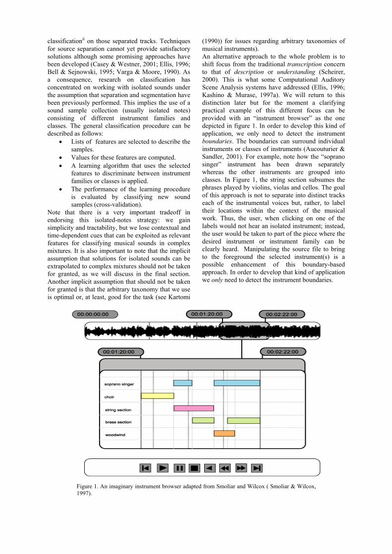
(1990)) for issues regarding arbitrary taxonomies of musical instruments). An alternative approach to the whole problem is to shift focus from the traditional transcription concern to that of description or understanding (Scheirer, 2000). This is what some Computational Auditory Scene Analysis systems have addressed (Ellis, 1996; Kashino & Murase, 1997a). We will return to this distinction later but for the moment a clarifying practical example of this different focus can be provided with an “instrument browser” as the one depicted in figure 1. In order to develop this kind of application, we only need to detect the instrument boundaries. The boundaries can surround individual instruments or classes of instruments (Aucouturier & Sandler, 2001). For example, note how the “soprano singer” instrument has been drawn separately whereas the other instruments are grouped into classes. In Figure 1, the string section subsumes the phrases played by violins, violas and cellos. The goal of this approach is not to separate into distinct tracks each of the instrumental voices but, rather, to label their locations within the context of the musical work. Thus, the user, when clicking on one of the labels would not hear an isolated instrument; instead, the user would be taken to part of the piece where the desired instrument or instrument family can be clearly heard. Manipulating the source file to bring to the foreground the selected instrument(s) is a possible enhancement of this boundary-based approach. In order to develop that kind of application we only need to detect the instrument boundaries.

Figure 1. An imaginary instrument browser adapted from Smoliar and Wilcox ( Smoliar & Wilcox,1997).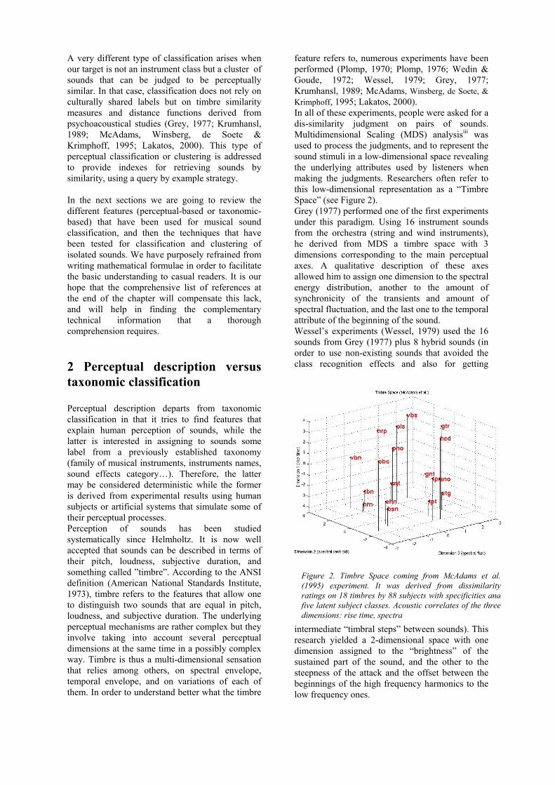

A very different type of classification arises when our target is not an instrument class but a cluster of sounds that can be judged to be perceptually similar. In that case, classification does not rely on culturally shared labels but on timbre similarity measures and distance functions derived from psychoacoustical studies (Grey, 1977; Krumhansl, 1989; McAdams, Winsberg, de Soete & Krimphoff, 1995; Lakatos, 2000). This type of perceptual classification or clustering is addressed to provide indexes for retrieving sounds by similarity, using a query by example strategy. In the next sections we are going to review the different features (perceptual-based or taxonomic-based) that have been used for musical sound classification, and then the techniques that have been tested for classification and clustering of isolated sounds. We have purposely refrained from writing mathematical formulae in order to facilitate the basic understanding to casual readers. It is our hope that the comprehensive list of references at the end of the chapter will compensate this lack, and will help in finding the complementary technical information that a thorough comprehension requires.

2 Perceptual description versus taxonomic classification Perceptual description departs from taxonomic classification in that it tries to find features that explain human perception of sounds, while the latter is interested in assigning to sounds some label from a previously established taxonomy (family of musical instruments, instruments names, sound effects category…). Therefore, the latter may be considered deterministic while the former is derived from experimental results using human subjects or artificial systems that simulate some of their perceptual processes. Perception of sounds has been studied systematically since Helmholtz. It is now well accepted that sounds can be described in terms of their pitch, loudness, subjective duration, and something called ”timbre”. According to the ANSI definition (American National Standards Institute, 1973), timbre refers to the features that allow one to distinguish two sounds that are equal in pitch, loudness, and subjective duration. The underlying perceptual mechanisms are rather complex but they involve taking into account several perceptual dimensions at the same time in a possibly complex way. Timbre is thus a multi-dimensional sensation that relies among others, on spectral envelope, temporal envelope, and on variations of each of them. In order to understand better what the timbre

feature refers to, numerous experiments have been performed (Plomp, 1970; Plomp, 1976; Wedin & Goude, 1972; Wessel, 1979; Grey, 1977; Krumhansl, 1989; McAdams, Winsberg, de Soete, & Krimphoff, 1995; Lakatos, 2000). In all of these experiments, people were asked for a dis-similarity judgment on pairs of sounds. Multidimensional Scaling (MDS) analysisiii was used to process the judgments, and to represent the sound stimuli in a low-dimensional space revealing the underlying attributes used by listeners when making the judgments. Researchers often refer to this low-dimensional representation as a “Timbre Space” (see Figure 2). Grey (1977) performed one of the first experiments under this paradigm. Using 16 instrument sounds from the orchestra (string and wind instruments), he derived from MDS a timbre space with 3 dimensions corresponding to the main perceptual axes. A qualitative description of these axes allowed him to assign one dimension to the spectral energy distribution, another to the amount of synchronicity of the transients and amount of spectral fluctuation, and the last one to the temporal attribute of the beginning of the sound. Wessel’s experiments (Wessel, 1979) used the 16 sounds from Grey (1977) plus 8 hybrid sounds (in order to use non-existing sounds that avoided the class recognition effects and also for getting

intermediate “timbral steps” between sounds). This research yielded a 2-dimensional space with one dimension assigned to the “brightness” of the sustained part of the sound, and the other to the steepness of the attack and the offset between the beginnings of the high frequency harmonics to the low frequency ones.

Figure 2. Timbre Space coming from McAdams et al. (1995) experiment. It was derived from dissimilarity ratings on 18 timbres by 88 subjects with specificities and five latent subject classes. Acoustic correlates of the three dimensions: rise time, spectra

Krumhansl (1989) used 21 FM-synthesis sounds from Wessel, Bristow & Settel (1987), mainly sustained harmonic sounds. She found the same results as Grey, but assigned the third dimension to something called “spectral flux” that was supposed to be related to the variations of the spectral content along time. McAdams et al. (1995), also used also these 21 FM-synthesis sounds in a new experiment and tested a new MDS technique that estimates the latent classes of subjects, instrument specificity values, and separate weights for each class. Compared to Krumhansl’s results, they confirmed the assignment of one dimension to the attack-time, another to the spectral centroid, but they did not confirm the “spectral flux” for the last dimension. Lakatos’ experiment (2000) used 36 natural sounds from the McGill University sound library, both wind and string (17) and percussive (18) sounds. The goal of this experiment was to extend the timbre space to percussive and mixed percussive/sustained sounds. This yields a two dimensional space and a three dimensional space. The conclusion of the experiment is that, except for spectral centroid and rise time, additional perceptual dimensions exist but their precise acoustic correlates are context dependent and therefore less prominent. An interesting practical application of this similarity-based research is that of setting up a given orchestration with some set of reference sound samples and then substituting some of them without radically changing the orchestration. Practical reasons for doing query-by-similarity of sound samples could include performance rights or copyrights issues, sample format compatibility, etc. Working examples of the timbre similarity approach are, for example, the Soundfisher system developed by Musclefishiv, and the Studio On Line developed by IRCAMv. Soundfisher, recently incorporated as a plug-in into a commercial video-logger called Virage, is designed to perform the classification, indexing and search of sounds in general, though it can be used in a music context. The initial versions of Soundfishervi (Keislar, Blum, Wheaton & Wold, 1995) did not yield an explicit class decision but, rather, generated a list of mathematically similar sounds. Some kind of class decision procedure, however, seems to have been recently implemented (Keislar, Blum, Wheaton & Wold, 1999). The Soundfisher system implicitly implements the assumption that what is mathematically similar can be also considered perceptually similar; in other words, that the computed features accurately represent perceptual dimensions, an assumption that contradicts most empirical studies. In contrast, Studio On Line computes similarity by using features that have been extracted under the paradigm of the above-

cited perceptual similarity psychoacoustical experiments. The interested reader can find in Peeters, McAdams & Herrera (2000) a recent validation of the psychoacoustical approach in the context of MPEG-7.

3. Relevant features for classification

3.1 Types of features The term feature denotes a quantity or a qualityvii describing an object of the world. In the realm of signal processing and pattern recognition, objects are usually described by using vectors or lists of features. Features are also known as attributes or descriptors. Audio signal features are usually computed directly from the signal, or from the output yielded by transformations such as the Fast Fourier Transform or the Wavelet Transform. These audio signal features are usually computed every few milliseconds, for a very short segment of audio samples, in order to grasp their micro-temporal evolution. Macro-temporal evolution features can also be computed by using a longer segment of samples (e.g. attack time, vibrato rate…), or by summarizing micro-temporal values (e.g. averages, variances…). A systematic taxonomy of features is outside the scope of this paper; nevertheless we could distinguish features at least according to four points of view: 1. The steadiness or dynamicity of the feature,

i.e. the fact that the features represent a value extracted from the signal at a given time, or a parameter from a model of the signal behavior along time (mean, standard deviation, derivative or Markov model of a parameter);

2. The time extent of the description provided by the features: some description applies to only part of the object (e.g. description of the attack of the sound), whereas other apply to the whole signal (e.g. loudness);

3. The “abstractness”, i.e. what does the feature represent (e.g. cepstrum and linear prediction are two different representation and extraction techniques for representing spectral envelope, but probably the former one can be considered as more abstract than the latter)

4. The extraction process of the feature. According to this point of view, we could further distinguish: • Features that are directly computed on the

waveform data as, for example, zero-crossing rate (the rate that the waveform changes from positive to negative values);

• Features that are extracted after performing a transform of the signal (FFT, wavelet…) as, for example, spectral

centroid (the “gravity center” of the spectrum);

• Features that relate to a signal model, as for example the sinusoidal model or the source/filter model;

• Features that try to mimic the output of the ear system (bark or erb bank filter output).

3.2. Relevant features for perceptual classification For each of the “timbre” experiments, people have tried to qualify the dimensions of these timbre spaces, the perceptual axes, in terms of ”brightness”, ”attack”, etc. Only recently attempts have been made to quantitatively describe these perceptual axes, i.e. relate the perceptual axes to variables or descriptors directly derived from the signal (Grey, 1978; Krimphoff, McAdams & Winsberg, 1994; Misdariis, Smith, Pressnitzer, Susini & McAdams, 1998). This quantitative description is done by finding the signal features that best explain the dis-similarity judgment. This is usually done using regression or multiple-regression between feature values and sound positions in the “timbre” space, and keeping only the features that yield the largest correlation. This makes the perceptual description framework different from taxonomic classification, since in the latter we’re not looking at features that “best explain” but at features that allow to “best discriminate” (between the considered classes). In the Grey and Gordon (1978) experiment, only one dimension correlated significantly with a perceptual dimension of their “timbre” space: the spectral centroid. Krimphoff et al. (1994) worked with Krumhansl’s space (1989) trying to find the quantitative parameters corresponding to its qualitative features and found, as Grey did, significant correlations with the spectral centroid, but also with the logarithm of the attack time and what they called the “spectral irregularity”, which is the average departure of the spectral harmonic amplitudes from a global spectral envelope. Krumhansl (1989) had labelled this dimension as “spectral flux”. Misdariis, Smith, Pressnitzer, Susini & McAdams, (1998) combined results coming from the Krumhansl (1989) and McAdams et al. (1995) experiments. They found the same features as Krimphoff did plus a new one that explained one dimension of McAdams et al. (1995) experiment: spectral flux defined here as the average of the correlation between amplitude spectra in adjacent time windows. Peeters et al. (2000) considered also the two above-cited experiments by Krumhansl and McAdams et al., called here “sustained harmonic sound space” as opposed to the “percussive sound space” coming from Lakatos (2000) experiment. Two methods

were used for the selection of the features, a “position” method, which tries to explain from the feature values the position of the sound in the timbre space, and a “distance” method, which tries to explain directly the perceived distance between sounds from a difference of feature values. From this study the following features, now part of the MPEG-7 standard, have been derived to describe the perceived similarity. For the “harmonic sustained sounds”: log-attack time, harmonic spectral centroid, harmonic spectral spread (the extent of the spectrum’s energy around the spectral centroid), harmonic spectral variation (the amount of variation of the spectrum energy distribution along time), and harmonic spectral deviation (the deviation of the spectrum harmonic from a global envelope). For the “percussive sounds”: log-attack time, temporal centroid (the temporal centre of gravity of the signal energy), and spectral centroid (the centre of gravity of the power spectrum of the whole sound). Another approach is the one taken by the company Muscle Fish in the development of the Soundfisher system (Wold, Blum, Keislar & Wheaton, 1966). In this case the selected features are not derived from experiments but they constitute a set that is similar to the one discussed above: loudness (rms value in dB), pitch, brightness (spectral centroid), bandwidth (spread of the spectrum around the spectral centroid), harmonicity (amount of energy of the signal explained by a periodic signal model)... In order to capture the temporal trend of the features, it is proposed to store their average, variance and auto-correlation values along time.

3.3. Relevant features for taxonomic classification Mel-Frequency Cepstrum Coefficients (hence MFCCs) are features that have proved useful for such speech processing tasks as, for example, speaker identification and speaker recognition (Rabiner & Juang, 1993). MFCCs are computed by taking the log of the power spectrum of a windowed signal, then non-linearly mapping the spectrum coefficients in a perceptually-oriented way (inspired by the Mel scale). This mapping is intended to emphasize perceptually meaningful frequencies. The Mel-weighted log-spectrum is then compacted into cepstral coefficients through the use of a discrete cosine transform. This transformation reduces the dimensionality of the representation without losing information (typically, the power spectrum may contain 256 values, whereas the MFCCs are usually less than 15). MFCCs provide a rather compact representation of the spectral envelope and are probably more musically meaningful than other common representations like Linear Predictive Coding coefficients or curve-fitting approximations to

spectrum. Despite these strengths, MFCCs by themselves can only convey information about static behavior and, as a consequence, temporal dynamics cannot be considered. Another important drawback is that MFCCs do not have an obvious direct interpretation, though they seem to be related (in an abstract way) with the resonances of instruments. Despite these shortcomings Marques (1999) used MFCCs in a broad series of classification studies. Eronen and Klapuri (2000) used Cepstral Coefficients (without the Mel scaling) and combined these features with a long list (up to 43) of complementary descriptors. Their list included, among others, centroid, rise and decay time, FM/AM rate and width, fundamental frequency and fundamental-variation-related features for onset and for the remainder of the note. In a more recent study, using a very large set of features (Eronen, 2001), the most important ones seemed to be the MFCCs, their standard deviations, and their deltas (differences between contiguous frames), the spectral centroid and related features, onset duration, and crest factor (specially for instrument family discrimination). There are ways, however, for adding temporal information into a MFCCS classification schema. For example, Cosi, De Poli & Prandoni (1994) created a Kohonen Feature Mapviii (Kohonen, 1995) using both note durations and the feature coefficients. The network then clustered and mapped the right temporal sequence into a bi-dimensional space. As a result, sounds were clustered in a human perceptual-like way (i.e. not into taxonomic classes but into timbrically similar conglomerates). Brown (1999) used cepstral coefficients from constant-Q transforms instead of taking them after FFT-transforms; she also clustered feature vectors in a way that the resulting clusters seemed to be coding some temporal dynamics. One of the most commonly used descriptors for musical, as well as non-musical, sound classification is energy. In (Kaminskyj & Materka, 1995), Root Mean Square (RMS) energy was used for classifying 4 different types of instruments with a neural network. In an additional, but apparently unfinished extension of this work (Kaminskyj & Voumard, 1996), the authors also included brightness, spectral onset asynchrony, harmonicity and MFCCs. In a more recent and comprehensive work (Kaminskyj, 2001) the main author used the RMS envelope, the Constant-Q frequency spectrum, and a set of spectral features derived from Principal Component Analysis (PCA from now on). PCA is commonly used to reduce dimensionality of complex data sets with a minimum loss of information. In PCA data is projected into abstract dimensions that are contributed with different –but partially related- variables. Then PCA calculates which projections, amongst all possible, are the best for representing the structure of data. The projections are chosen so that the maximum

variability of the data is represented using the smallest number of dimensions. In this specific research, the 177 spectral bins of the Constant-Q were reduced, after PCA, to 53 “abstract” features without any significant loss in discriminative power. Martin and Kim (Martin & Kim, 1998) exemplified the idea of testing very long lists of features and then selecting only those shown to be most relevant for performing classifications. Martin and Kim worked with log-lag correlograms to better approximate the way our hearing system processes sonic information. They examined 31 features to classify a corpus of 14 orchestral wind and string instruments. They found the following features to be the most useful: vibrato and tremolo strength and frequency, onset harmonic skew (i.e., the time difference of the harmonics to arise in the attack portion), centroid related measures (e.g., average, variance, ratio along note segments, modulation), onset duration, and select pitch related measures (e.g., value, variance). The authors noted that the features they studied exhibited non-uniform influences, that is, some features were better at classifying some instruments and instrument families and not others. In other words, features could be both relevant and non-relevant depending on the context. The influence of non-relevant features degraded the classification success rates between 7% and 14%. This degradation is an important theoretical issue (Blum & Langley, 1997) that unfortunately has been overlooked by the majority of studies we have reviewed. It should be noted that there are some classification techniques that also provide some indication about the relevance of the involved features. This is the case with Discriminant Analysis (see section 4.2.3). Using this technique “backward” deletion and “forward” addition of features can be used in order to settle into a good (though sometimes suboptimal) set. Agostini, Longari, and Pollastri ( 2001) have used this method for reducing their original set of eighteen features to the eight ones that best separate the groups. The best features were: inharmonicity mean, centroid mean and standard deviation, harmonicity energy mean, zero-crossing rate, bandwidth mean and standard deviation, and standard deviation of harmonic skewness. Spectral flatness is a feature that has been recently used in the context of MPEG-7 (Herre, Allamanche & Hellmuth, 2001) for robust retrieval of song archives. It is a “newcomer” in musical instrument classification but can be quite useful because it indicates how flat (i.e. “white-noisy”) the spectrum of a sound is. Our current work indicates that it can also be a good descriptor for percussive sound classification (Herrera, Yeterian & Gouyon, 2002). Jensen and Arnspang (1999) used amplitude, brightness, tristimulus, amplitude of odd partials, irregularity of spectral envelope, shimmer and jitter measures, and inharmonicity, for studying the classification of 1500 sounds from 7 instruments.

Jensen (1999), using PCA, had earlier identified these features as the most relevant from an initial set of 20 and indicated 3 relevant dimensions that could summarize the most important features. He labeled these, in decreasing order of importance, “spectral envelope”, “(temporal) envelope”, and “noise”. Kashino and Murase (1997b) applied PCA to the instrument classification problem: 41 features were reduced to 11. PCA, in the context of sound classification, can be also found in the works of Sandell and Martens (1995), and Rochebois and Charbonneau, (1997). Less compact representations for temporal or spectral envelopes can be found in Fragoulis, Avaritsiotis, and Papaodysseus (1999), who used the slope of the first five partials, the time delay in the onset of these partials, and the high-frequency energy. Cemgil and Gürgen (1997)) also used a set of harmonics (the first twelve) as discriminative features in their neural networks study. Apart from PCA, another useful method for reducing the dimensions of the feature selection problem is the application of Genetic Algorithms (GAs). GAs are modeled on the processes that drive the evolution of gene populations (e.g., crossover, mutation, evaluation of fitness, and selection of the best adapted). GAs have a property called implicit search, which means that near-optimal combinations of genes can be found without explicitly evaluating all possible combinations. GAs have been used in other musical contexts (e.g., sound synthesis and music composition) but the only known application to sound classification has been that of Fujinaga, Moore, and Sullivan (1998) where GAs were used to discover the best feature set. From an initial set of 352 features, their GA determined that the centroid, fundamental frequency, energy, standard deviation and skewness of spectrum, and the amplitudes of the first two harmonics were the best features to achieve a successful classification rate. In a more recent work (Fujinaga & MacMillan, 2000), two additional significant features were reported: spectral irregularity and a modified version of tristimulus. Unfortunately, the selection of best features was heavily instrument-dependent. This problematic dependence has been also noted by other studies. The intensive study of feature selection performed by Kostek (1998) represents another interesting approach. Kostek thoroughly examined approximately a dozen features. Examined features include, for example, energy of fundamental and of sets of partials, brightness, odd/even partials ratio, tristimulus-like features, and time delays of partials with respect to the fundamental. Kostek also explored, in other studies, the use of features derived from Wavelet Transforms instead of FFT-derived features. She found that the latter provided slightly better results than the former. One of the more interesting aspects of Kostek’s work is her use of rough sets (Pawlak, 1982; Pawlak,

1991). Rough sets are a technique that was developed in the realm of knowledge-based discovery systems and data mining. Rough sets are implemented with the aim of classifying objects and then evaluating the relevance of the features used in the classification process. An elementary introduction to rough sets can be found in (Pawlak, 1998). We will return later with a fuller explication of rough sets. Applications of the rough sets technique to different problems, including those of signal processing, can be found in (Czyzewski, 1998). Polkowski and Skowron (1998) present a thoughtful discussion of software tools implementing this kind of formalisms. Several studies by Kostek and her collaborators (Kostek, 1995; Kostek, 1998; Kostek, 1999; Kostek & Czyzewski, 2001), and by Wieckzorkowska (1999b), used rough sets for reducing a large initial set of features for instrument classification. Wieckzorkowska’s study provides the clearest example of set reduction using rough sets. She found that a starting set of sixty-two spectral and temporal features describing attack, steady state, and release of sounds could be further reduced to a set of sixteen features. Examples of the more significant features include: tristimulus, energy of 5th, 6th and 7th harmonics, energy of even partials, energy of odd partials, the most deviating of the lower partials, mean frequency deviation for low partials, brightness, and energy of high partials. Temporal differences between values of the same feature have been rarely used in the reviewed studies. Soundfisher, the commercial system mentioned earlier, incorporates temporal differences alongside such basic features as loudness, pitch, brightness, bandwidth, and MFCCs (Wold, Blum, Keislar & Wheaton, 1999). The Fujinaga or Eronen studies (cited above) have also incorporated temporal differences. To summarize this section, there are two inter-related factors that influence the success of feature-based identification and classification tasks. First, one must determine, and then select, the most discriminatory features from a seemingly infinite number of candidates. Second, one must reduce the number of applied features in order to make the resultant calculations tractable. We might intuitively conclude that using more than fifteen or twenty features seems to be a non-optimal strategy for attempting automatic classification of musical instruments. In order to settle into a short feature list, reliable data reduction techniques should be used. PCA and some types of Discriminant Analysis (both explained below) are robust and relatively easy to compute. Other techniques such as Kohonen maps, Genetic Algorithms, Rough Sets, etc., might yield better results when appropriate parameters and data are selected, but are inherently more complex. It is also clear that

there are some features that are discriminative only for certain types of instruments, and that not only temporal and spectral features, but also their temporal evolution, should be considered.

4. Techniques for sound classification

4.2. Perceptual-based clustering and classification Retrieving sounds from a database by directly selecting signal features as those cited in the previous section is not a friendly task. As a consequence, exploiting relationships between them and high-level descriptions such as class or property (roughness, brightness) is required. A different way of retrieving sounds is by providing examples that are similar to what we are searching for; this is known as “query by example”. A specific kind of “query by example” is the one based on similarity of perception of sounds, instead of being based on sound categories. Leaving pitch, loudness and duration apart, this points directly to the notion of timbre and therefore to “timbre similarity”. Several authors have proposed a measure of timbre similarity that has been derived from psycho-acoustical experiments (see section 2). This measure allows one to approximate the average judgment of perceived similarity obtained from people’s dissimilarity judgments between pairs of sounds. In order to do that, features or combinations of them, are used, with a possible weighting, to position the sound into a multi-dimensional space. Giving two sounds, a measure of timbre similarity can be approximated. Therefore, for a given target sound, it is possible to find in a database the one that “sounds” the closest to the target. Misdariis et al. (1998) derived such a similarity measure approximation from Krumhansl (1989) and McAdams et al. (1995) experiments. Its formulation uses four features: log-attack-time, spectral centroid, spectral irregularity and spectral flux. Use of the similarity measure proposed by Misdariis et al. (1998) can be found, for example, in the search engine of IRCAM’s “Studio On Line” sound database. Peeters et al. (2000) proposed a new approximation adding the new feature “spectral spread”. They also proposed an equivalent approximation for percussive sounds derived from the Lakatos (2000) experiment. This latter uses the log-attack time, the spectral centroid and the temporal centroid. A still remaining problem concerns the applicability of such a timbre similarity measure for sounds belonging to different families (as for example comparing a sustained harmonic sound –

i.e. an oboe sound- with a percussive sound –i.e. a snare sound-). Current research is trying to construct a meta-timbre-space allowing such comparison between sounds belonging to different sound classes. Another kind of approach is that of Feiten and Günzel (1994), Cosi, De Poli, and Lauzzana (1994), or Spevak and Polfreman (2000). Signal features used in these works try to take into account the properties of human perception: MFCCs, Loudness critical-band rate time patterns, Lyon’s cochlear model, Gamma filter banks, etc. These features are then used in order to construct, automatically, what is called a “physical timbre space”. The “physical timbre space” aims at being the equivalent to usual timbre spaces but derived from signal features instead of from dissimilarity judgments yielded by human subjects in experimental conditions. A “physical timbre space” can be derived from signal features using various techniques: Hierarchical Clustering, Multi-Dimensional Scaling analysis (see section 2), Kohonen Feature Maps (a.k.a. Self Organizing Maps, see note 8), or Principal Component Analysis (see section 3.3). Prandoni (1994) and De Poli and Prandoni (1997) used a combination of MFCCs, Self-Organized Maps, and PCA analysis. The authors applied this framework to the sounds of Wessel et al. (1987) and found that brightness and spectral slope are the features that best explain two of its “physical timbre space” axes. Prandoni (1994) used the barycentre of the representation of each sound family in a feature (MFCCs) space. Using MDS and Herarchical Clustering analysis he found similar results than Grey did, and assigned the first two axes of his space to brightness and to something called “presence”, which is a measure of the energy inside the 800 Hz. region. In these two studies the obtained spaces were compared to usual timbre spaces coming from human experiments such as the above cited (sections 2 and 3.2). In Feiten and Günzer (1994), and Spevak and Polfreman (2000)), the obtained spaces are used to make a temporal model of the sound evolution. The former authors define two sound feature maps (SFM). The first SFM is derived directly from a Kohonen Feature Map training using the MFCCs. This SFM, called the Steady State SFM, represents the steady parts of the sounds. Each sound is then represented by a trajectory between the states of the Steady State SFM. A Dynamic State SFM is then computed from these trajectories. The latter authors, on the other hand, make a comparison between different feature sets (Lyon’s cochlear model, Gamma Tone filterbank and MFCCs), considering their abilities to represent clear and separated trajectories in the SFM. They conclude that the best feature set is the Gamma Tone

filterbank combined with Meddis’s inner hair cell model.

4.3. Taxonomic classification In this section we are going to present different techniques that have been used for learning to classify isolated musical notes into instrument or music family categories. Although we have focused on the testing phase success rate as a way for evaluating them, we have to be cautious because other factors (number of instances used in the learning phase, number of instances used in the testing phase, testing procedure, number of classes to be learned, etc.) may have a large impact on the results.

K-Nearest Neighbors

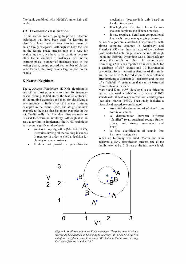
The K-Nearest Neighbours (K-NN) algorithm is one of the most popular algorithms for instance-based learning. It first stores the feature vectors of all the training examples and then, for classifying a new instance, it finds a set of k nearest training examples in the feature space, and assigns the new example to the class that has more examples in the set. Traditionally, the Euclidean distance measure is used to determine similarity. Although it is an easy algorithm to implement, the K-NN technique has several significant drawbacks:

• As it is a lazy algorithm (Mitchell, 1997), it requires having all the training instances in memory in order to yield a decision for classifying a new instance.

• It does not provide a generalization

mechanism (because it is only based on local information).

• It is highly sensitive to irrelevant features that can dominate the distance metrics.

• It may require a significant computational load each time a new query is processed.

A k-NN algorithm classified 4 instruments with almost complete accuracy in Kaminskyj and Materka (1995), but the small size of the database (with restricted note range to one octave, although including different dynamics) was a drawback for taking this result as robust. In recent years Kaminskyj (2001) has reported hit rates of 82% for a database of 517 sounds and 19 instrumental categories. Some interesting features of this study are the use of PCA for reduction of data obtained after applying a Constant Q Transform and the use of a “reliability” estimation that can be extracted from confusion matrices. Martin and Kim (1998) developed a classification system that used a k-NN on a database of 1023 sounds with 31 features extracted from cochleagrams (see also Martin (1999). Their study included a hierarchical procedure consisting of:

• An initial discrimination of pizzicati from continuous notes.

• A discrimination between different “families” (e.g., sustained sounds further divided into strings, woodwind, and brass),

• A final classification of sounds into instrument categories.

When no hierarchy was used, Martin and Kim achieved a 87% classification success rate at the family level and a 61% rate at the instrument level.

3A B V

2 BB 2 A

B A 1 A

0 1 2 3V1

Figure 3. An illustration of the K-NN technique. The point marked with a star would be classified as belonging to category “B” when K=3 (as two out of its 3 neighbours are from class “B”; but note that in case of using K=5 classification would be “A”.

Use of the hierarchical procedure increased the accuracy at the instrument level to 79% but it degraded the performance at the family level to 79%. In the case of not including the hierarchical procedure, performance figures were lower than the ones they obtained with a Bayesian classifier. Similar results (65% for 27 instrument classes; 77% for a two-level 6-element hierarchy) were reported by Agostini et al. (2001). In this report, the k-NN technique compared unfavorably against Discriminant Functions and also against Support Vector Machines. Eronen and Klapuri (2000) used a combination of k-NN and a Gaussian classifier (which was only used for rough discrimination between pizzicati and sustained sounds) for classifying 1498 samples into specific instrumental families or specific instrument labels. Using a system architecture very similar to Martin and Kim’s hierarchy –wherein sounds are first classified in broad categories and then the classification is refined inside that category- they reported success rates of 75% in individual instrument classification and 94% for family classification. They also reported a small accuracy improvement by only using the best features for each instrument and no hierarchy at all (80%). A quite surprising result is the extreme degradation of performance results (35%) that has been reported in a more recent paper (Eronen, 2001). The explanation may be found in several facts: they used a larger and more varied database (5286 sounds coming from different collections) and more restrictive cross-validation methods (the test phase used sounds that were completely excluded from the learning set). A possible enhancement of the K-NN technique, which includes the weighting of each feature according to its particular relevance for the task, has been used by the Fujinaga team (Fujinaga et al., 1998; Fujinaga, 1998; Fraser & Fujinaga, 1999; Fujinaga & MacMillan, 2000). In a series of three experiments using over 1200 notes from 39 different instruments, the initial success rate of 50%, observed when only the spectral shape of steady-state notes was used, increased to 68% when tristimulus, attack position, and features of the dynamically changing spectrum envelope (i.e., the change rate of the centroid) were added. In their last paper, a real-time version of this system was reported. The k-NN literature—including the works of such research leaders as Martin and Fujinaga—consistently reports accuracy rates around 80%. Provided that the feature selection has been optimized with genetic or other optimization techniques, one can thus interpret the 80% accuracy value as an estimation of the limitations of the K-NN algorithm. Therefore, more powerful techniques should be explored.

Naive Bayesian Classifiers

A Naïve Bayesian Classifier (NBC) incorporates a learning step in which the probabilities for the classes and the conditional probabilities for a given feature and a given class are estimated. Probability estimates for each of these are based on their frequencies as found in a collection of training data. The set of these estimates corresponds to the learned hypothesis, which is formed by simply counting the occurrences of various data combinations within the training examples. Each new instance is classified based upon the conditional probabilities calculated during the learning phase. This type of classifier is called naïve because it assumes the independence of the features. Brown (1999) used the NBC technique in conjunction with 18 Cepstral Coefficients computed after a constant Q transform. After clustering the feature vectors with a K-means algorithm, a Gaussian mixture model from their means and variances was built. This model was used to estimate the probabilities for a Bayesian classifier. It then classified 30 short sounds of oboe and sax with an accuracy rate of 85%. In a more recent paper (Brown, Houix & McAdams, 2001) she and her collaborators reported similar hit rates for four classes of instruments (oboe, sax, clarinet and flute); these good results were replicated for different types of descriptors (cepstral coefficients, bin-to-bin differences of the constant-Q spectrum, and autocorrelation coefficients). Martin (1999) enhanced a similar Bayesian classifier with context-dependent feature selection procedures, rule-one-out category decisions, beam search, and Fisher discriminant analysis, to estimate the maximum a priori probabilities. In (Martin & Kim, 1998), performance of this system was better than that of a K-NN algorithm at the instrument level with a 71% accuracy rate and equivalent to it at the family level with 85% accuracy rate. Kashino and his team (1995) have also used a Bayesian classifier in their CASA system. Their implementation is reported to be able to classify, and even separate, five different instruments: clarinet, flute, piano, trumpet and violin. Unfortunately, no specific performance data are provided in their paper.

Discriminant Analysis

Classification using categories or labels that have been previously defined can be done with the help of Discriminant Analysis (DA), a technique that is related to multivariate analysis of variance (MANOVA) and multiple regression. DA attempts to minimize the ratio of within-class scatter to the

between-class scatter and builds a definite decision region between the classes. It provides linear, quadratic or logistic functions of the variables that "best" separate cases into two or more predefined groups. DA is also useful for determining which are the most discriminative features and the most similar/dissimilar groups. Surprisingly there have been very few studies using these techniques. Martin and Kim (1998)) made limited use of this method when they used a linear DA to estimate the mean and variance of the Gaussian distributions of each class to be fed into an enhanced naive Bayesian classifier. More recently Agostini et al. (2001) have found that a set of quadratic discriminant functions outperformed even Support Vector Machines (93% versus 70% hit rates) in classifying 1007 tones from 27 musical instruments with a very small set of descriptors. In our laboratory we carried out, some time ago, an unpublished study with 120 sounds from 8 classes and 3 families in which we got a 75% accuracy using also quadratic linear discriminant functions in two steps (sounds were first assigned to a family, and then they were specifically classified). As the features we used were not optimized for instrument classification but for perceptual similarity classification, it would be reasonable to expect still better results when including other more task-specific features. In a more recent work (Herrera et al., 2002) that used a database of 464 drum sounds (kick, snare, hihat, tom, cymbals) and an initial set of more than thirty different features, we got hit rates higher than 94% with four canonical Discriminant functionsix that combined 18 features comprising some MFCCs, attack and decay descriptors, and relative energies in some selected bands.

Higher Order Statistics

When signals have Gaussian density distributions, we can describe them thoroughly with such second order measures as the autocorrelation function or the spectrum. In the case of noisy signals such as engine noises of sound effects, the variations in the spectral envelope do not allow a good signal characterisation and matching. A method to match signals using a variant of matched filter using polyspectral matching was presented in (Dubnov & Tishby, 1997), and it could be specifically useful for the classification of sounds from percussive instruments. There are some authors who claim that musical signals, because they have been generated through non-linear processes, do not fit a Gaussian distribution. In that case, using higher order statistics or polyspectra, as for example skewness of bispectrum and kurtosis of trispectrum, it is possible to capture all information that could be lost if using a simpler Gaussian model. With these

techniques, and using a Maximum Likelihood classifier, Dubnov, Tishby, and Cohen (1997) have showed that discrimination between 18 instruments from string, woodwind and brass families is possible. Unfortunately the detailed data that is presented there comes from a classification experiment that used machine and other types of non-instrumental sounds. Acoustic justification for differences in kurtosis among families of instruments was provided in (Dubnov & Rodet, 1997). The measure of kurtosis was shown to correspond to the phenomenon of phase coupling, which implies coherence in phase fluctuations among the partials.

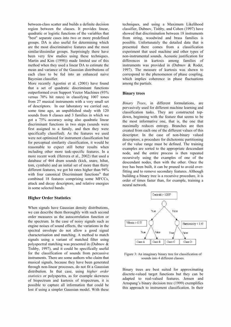
Binary trees

Binary Trees, in different formulations, are pervasively used for different machine learning and classification tasks. They are constructed top-down, beginning with the feature that seems to be the most informative one, that is, the one that maximally reduces entropy. Branches are then created from each one of the different values of this descriptor. In the case of non-binary valued descriptors, a procedure for dichotomic partitioning of the value range must be defined. The training examples are sorted to the appropriate descendant node, and the entire process is then repeated recursively using the examples of one of the descendant nodes, then with the other. Once the tree has been built, it can be pruned to avoid over-fitting and to remove secondary features. Although building a binary tree is a recursive procedure, it is order of times faster than, for example, training a neural network.

Figure 3: An imaginary binary tree for classification of

sounds into 4 different classes.

Binary trees are best suited for approximating discrete-valued target functions but they can be adapted to real-valued features. Jensen and Arnspang’s binary decision tree (1999) exemplifies this approach to instrument classification. In their

system, the trees are constructed by asking a large number of questions designed in each case to divide the data into two sets (e.g., “Is attack time longer than 60 ms?). Goodness of split (e.g., average entropy) is calculated and the question that renders the best goodness is chosen. Once the tree has been built using the learning set, it can be used for classifying new sounds because each leaf corresponds to one specific class. The tree can also be used for making explicit rules about which features better discriminate one instrument from another. Unfortunately, detailed results regarding the classification of new sounds have not yet been published. Consult Jensen’s thesis (1999), however, for his discussion of log-likelihood classification functions. Wieczorkowska (1999a) used a binary tree approach, called the C4.5 algorithm (Quinlan, 1993), to classify a database of 18 classes and 62 features. Accuracy rates varied between 64% and 68% depending on the test procedure applied. In our above-mentioned drum sounds classification study (Herrera et al., 2002) we obtained slightly better figures (83% of hit rates) using the C4.5 algorithm for classifying nine different classes of instruments. A final example of a binary tree for audio classification, although not specifically tested with musical sounds, is that of Foote (1997). His tree-based approach uses MFCCs and supervised vector quantization to partition the feature space into a number of discrete regions. Each split decision in the tree involves comparing one element of the vector with a fixed threshold that is chosen to maximize the mutual information between the data and the associated human-applied class labels. Once the tree is built, it can be used as a classifier by computing histograms of frequencies of classes in each leaf of the tree; histograms are similarly generated for the test sounds then compared with tree-derived histograms.

Artificial Neural Networks

An Artificial Neural Network (ANN) is an information processing structure that is composed of a large number of highly interconnected processing elements—called neurons or units—working in unison to solve specific problems. Neurons are grouped into layers (usually called input, output, and hidden) that can be interconnected through different connectivity patterns. An ANN learns complex mappings between input and output vectors by changing the weights that interconnect neurons. These changes may proceed either supervised or unsupervised. In the supervised case, a teaching instance is presented to the ANN, it is asked to generate an output, this out is then compared with an expected

“correct” output, and the weights are consequently changed in order to minimize future errors. In the unsupervised case, the weights “settle” into a pattern that represents the collection of input stimulus. A very simple feedforward network with a backpropagation training algorithm was used in (Kaminskyj & Materka, 1995). The network (a system with 3 input units, 5 hidden units, and 4 output units) learned to classify sounds from 4 very different instruments—piano, marimba, accordion and guitar—with an accuracy rate as high as 97%. Slightly better results were obtained, however, using a simpler K-NN algorithm. A three-way evaluative investigation involving a multilayer network, a time-delayed network, and a hybrid self-organizing network/radial basis function (see note 5) can be found in (Cemgil & Gürgen, 1997). Although very high success rates were found (e.g., 97% for the multilayer network, 100% for the time-delay network, and 94% for the self-organizing network) it should be noted that the experiments used only 40 sounds from 10 different classes with the pitch range limited to one octave. Implementations of self-organizing maps (Kohonen, 1995) can be found in (Feiten & Günzel, 1994; Cosi, De Poli & Lauzzana, 1994; Cosi et al., 1994; Toiviainen et al., 1998). All these studies used some kind of human auditory pre-processing simulation to derive the features that were fed to the network. Each then built a map and evaluated its quality by comparing the network clustering results to those human-based sound similarity judgments (Grey, 1977; Wessel, 1979). From their maps and their comparisons they advance timbral spaces to be explored, or confirm/reject theoretical models that explain the data. We must note, however, that the classification we get from self-organizing maps has not traditionally been directly usable for instrument recognition, as the maps are not provided with any a priori label to be learned (i.e., no instrument names). Nevertheless, there are several promising mechanisms being explored for associating the output clusters to specific labels (e.g., the radial basis function used by Cemgil, (see above). The ARTMAP architecture (Carpenter, Grossberg & Reynolds, 1991) is another means to implement this strategy. ARTMAP has a very complex topology including a couple of associative memory subsystems and also an “attentional” subsystem. Fragoulis et al. (1999) successfully used an ARTMAP for the classification of 5 instruments with the help of only ten features: slopes of the first five partials, time delays of the first 4 partials relative to the fundamental, and high frequency energy. The small 2% error rate reported was attributed to neglecting different playing dynamics in the training phase. Kostek’s (1999) is the most exhaustive study on instrument classification using neural networks.

Kostkek’s team has carried out several studies (Kostek & Krolikowski, 1997; Kostek & Czyzewski, 2000; Kostek & Czyzewski, 2001) on network architecture, training procedures, and number and type of features, although the number of classes to be classified has been always too small. They have used a feedforward NN with one hidden layer. Initially their classes were instruments with somewhat similar sounds: trombone, bass trombone, English horn and contrabassoon. In last papers more categories (double bass, cello, viola, violin, trumpet, flute, clarinet…) have been added to the tests. Accuracy rates higher than 90% were achieved for different sets of four classes, although the results varied depending on the types of training and descriptors used. Some ANN architectures are capable of approximating any function. This attribute makes neural networks a good choice when the function to be learned is not known in advance, or it is suspected to be nonlinear. ANN’s do have some important drawbacks, however, that must be considered before they are implemented: the computation time for the learning phase is very long, adjustment of parameters can be tedious and prohibitively time consuming, and data over-fitting can degrade their generalization capabilities. It is still an open question whether ANN’s can outperform simpler classification approaches. They do, however, exhibit one strong attribute that recommends their use: once the learning phase is completed, the classification decision is very fast when compared to other popular methods such as k-NN.

Support Vector Machines

SVMs are based on statistical learning theory (Vapnik, 1998). The basic training principle underlying SVMs is finding the optimal linear hyperplane such that the expected classification error for unseen test samples is minimized (i.e., they look for good generalization performance). According to the structural risk minimization inductive principle, a function that classifies the training data accurately, and which belongs to a set of functions with the lowest complexity, will generalize best regardless of the dimensionality of the input space. Based on this principle, a SVM uses a systematic approach to find a linear function with the lowest complexity. For linearly non-separable data, SVMs can (nonlinearly) map the input to a high dimensional feature space where a linear hyperplane can be found. This mapping is done by means of a so-called kernel function (denoted by φ in Figure 4). Although there is no guarantee that a linear solution will always exist in the high dimensional space, in practice it is quite feasible to construct a

working solution. In other words, it can be said that training a SVM is equivalent to solving a quadratic programming with linear constraints and as many variables as data points. Anyway, SVM present also some drawbacks: first, there is a risk of selecting a non-optimal kernel function; second, when there are more than two categories to classify, the usual way to proceed is to perform a

concatenation of two-class learning procedures; and third, the procedure is computationally intensive.

Figure 4. In SVM’s the Kernel function f maps the inputspace (where discrimination of the two classes ofinstances is not easy to be defined) into a so-called featurespace, where a linear boundary can be set between the twoclasses

Marques (1999) used an SVM for the classification of 8 solo instruments playing musical scores from well-known composers. The best accuracy rate was 70% using 16 MFCCs and 0.2 second sound segments. When she attempted classification on longer segments an improvement was observed (83%). There were, however, two instruments found to be very difficult to classify: trombone and harpsichord. Another noteworthy feature of this study was the use of truly independent sets for the learning and for the testing consisting mainly of “solo” phrases from commercial recordings. Agostini et al. have reported quite surprising results (Agostini et al., 2001). In their study an SVM performed marginally better than (Linear) Canonical Discriminant functions and also better than k-NN’s, but not nearly as good as a set of Quadratic Discriminant Functions (see section 4.2.3). Some promising applications of SVM that are related to music classification but are not specific to music instrument labelling can be found in Li & Guo (2000), Whitman, Flake and Lawrence (2001), Moreno and Rifkin (2000), or Guo, Zhang, and Li (2001).

Rough Sets

Rough sets are a novel technique for evaluating the relevance of the features used for description and classification. These are similar to, but should not

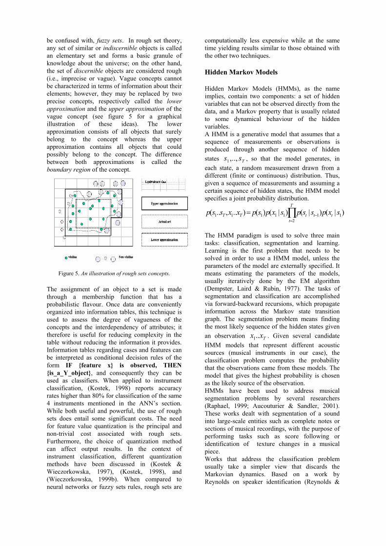
be confused with, fuzzy sets. In rough set theory, any set of similar or indiscernible objects is called an elementary set and forms a basic granule of knowledge about the universe; on the other hand, the set of discernible objects are considered rough (i.e., imprecise or vague). Vague concepts cannot be characterized in terms of information about their elements; however, they may be replaced by two precise concepts, respectively called the lower approximation and the upper approximation of the vague concept (see figure 5 for a graphical illustration of these ideas). The lower approximation consists of all objects that surely belong to the concept whereas the upper approximation contains all objects that could possibly belong to the concept. The difference between both approximations is called the boundary region of the concept.

Figure 5. An illustration of rough sets concepts.

The assignment of an object to a set is made through a membership function that has a probabilistic flavour. Once data are conveniently organized into information tables, this technique is used to assess the degree of vagueness of the concepts and the interdependency of attributes; it therefore is useful for reducing complexity in the table without reducing the information it provides. Information tables regarding cases and features can be interpreted as conditional decision rules of the form IF {feature x} is observed, THEN {is_a_Y_object}, and consequently they can be used as classifiers. When applied to instrument classification, (Kostek, 1998) reports accuracy rates higher than 80% for classification of the same 4 instruments mentioned in the ANN’s section. While both useful and powerful, the use of rough sets does entail some significant costs. The need for feature value quantization is the principal and non-trivial cost associated with rough sets. Furthermore, the choice of quantization method can affect output results. In the context of instrument classification, different quantization methods have been discussed in (Kostek & Wieczorkowska, 1997), (Kostek, 1998), and (Wieczorkowska, 1999b). When compared to neural networks or fuzzy sets rules, rough sets are

computationally less expensive while at the same time yielding results similar to those obtained with the other two techniques.

Hidden Markov Models

Hidden Markov Models (HMMs), as the name implies, contain two components: a set of hidden variables that can not be observed directly from the data, and a Markov property that is usually related to some dynamical behaviour of the hidden variables. A HMM is a generative model that assumes that a sequence of measurements or observations is produced through another sequence of hidden states , so that the model generates, in each state, a random measurement drawn from a different (finite or continuous) distribution. Thus, given a sequence of measurements and assuming a certain sequence of hidden states, the HMM model specifies a joint probability distribution.

Tss ,..,1

∏=

−=T

ttttTT sxpsspsxpspxxssp

21111111 )|()|()|()()..,..(

The HMM paradigm is used to solve three main tasks: classification, segmentation and learning. Learning is the first problem that needs to be solved in order to use a HMM model, unless the parameters of the model are externally specified. It means estimating the parameters of the models, usually iteratively done by the EM algorithm (Dempster, Laird & Rubin, 1977). The tasks of segmentation and classification are accomplished via forward-backward recursions, which propagate information across the Markov state transition graph. The segmentation problem means finding the most likely sequence of the hidden states given an observation . Given several candidate HMM models that represent different acoustic sources (musical instruments in our case), the classification problem computes the probability that the observations came from these models. The model that gives the highest probability is chosen as the likely source of the observation.

Txx ..1

HMMs have been used to address musical segmentation problems by several researchers (Raphael, 1999; Aucouturier & Sandler, 2001). These works dealt with segmentation of a sound into large-scale entities such as complete notes or sections of musical recordings, with the purpose of performing tasks such as score following or identification of texture changes in a musical piece. Works that address the classification problem usually take a simpler view that discards the Markovian dynamics. Based on a work by Reynolds on speaker identification (Reynolds &

Rose, 1995), several researchers considered a Gaussian Mixture Model (GMM) for computer identification of musical instruments (Brown, 1999; Marques, 1999). GMMs consider a continuous probability density of the observation, and model it as a weighted sum of several Gaussian densities. The hidden parameters in GMM are the mean vector, covariance matrix and mixture weight of the component densities. Parameter estimation is performed using an EM procedure or k-means. Using a GMM in an eight-instrument classification task, Marques reported an overall error rate of 5% for 32 Gaussians with MCCs as features. Brown performed a two-instrument classification experiment where she compared machine classification results with human perception for a set oboe and saxophone sounds. She reported a lower error rate for the computer than humans for oboe samples and roughly the same for the sax samples. Eronen and Klapuri (2000) also compare a GMM classifier to other classifiers for various features. In the HMM model for sound clips presented by Zhang and Kuo (1998a; 1999b) they use a continuous observation density probability distribution function (pdf) with various architectures of the Markov transition graphs. They also incorporate an explicit State Duration model (semi-markov model, (Rabiner, 1989) for modelling the possibility that d consecutive observations belong to the same state. Denote a complete parameter set of HMM as

, with A for the transition probability, B for the GMM parameters, D for duration pdf parameters and π for initial state distribution. In this model, two types of information are represented in the HMM: timbre and rhythm. Each kind of timbre is modelled by a state, and rhythm information is denoted by transition and duration parameters. The authors arrive at a three step learning procedure that first uses GMM for estimating B, then A is calculated from statistics of the state transitions and eventually D is estimated state by state, assuming a Gaussian density for the durations. This simplified procedure is not a strict HMM learning process and it is used to simplify the computational load of the learning stage. They report over 80% accurate classification rate for 50 sound clips, with misclassifications reportedly happening with classes of perceptually similar sounds, such as applause, rain, river and windstorm. The timbre of sound is described primarily by the frequency energy distribution that is extracted from short time spectrum. In their experiments, Zhang and Kuo employ a rather naive feature set for description of the timbre, that consist of log amplitude from a 128-point FFT vector (thus obtaining a 65 dimensional feature vector), calculated at

approximately 9 msec intervals. Depending on the type of sound that is analyzed, a partial or complete HMM models is employed. The simplest ones are single state sounds, and sounds that omit duration and transition information. These are used when every timbral state in the model can occur anywhere in time and for any duration. Second model includes transition probabilities, but without durations. The third (complete case) includes sounds such as footsteps and clock ticks, which carry both transition and duration information. An improvement to the timbral description was recently suggested by Casey and Westner (2001). Instead of using magnitude FFT, they suggest reduced rank spectra as a feature set for HMM classifier. After FFT analysis, singular value decomposition (SVD) is used to estimate a new basis for the data and, by discarding basis vectors with low eigenvalues, a data-reduction step is performed. Then the results are passed to independent component analysis (ICA

),,,( πλ DBA=

x), which imposes additional constraints on the output features. The resulting representation consists of a projection of a data into a lower-dimensional space with marginal distributions being approximately independent. They report a success rate of 92.65% for reduced-rank versus 60.61% for the full-rank spectra HMM classifier. Another variant of Markov modelling, but this time using explicit (not hidden) observations with arbitrary length Markov modelling was used by Dubnov and Rodet (1998). In this work a universal classifier is constructed using a discrete set of features. The features were obtained by clustering (vector quantization of) cepstral and cepstral derivative coefficients. The motivation for this model is a universal sequence classification method of Ziv-Merhav (Ziv & Merhav, 1993) that performs matching of arbitrary sequences with no prior knowledge of the source statistics and having an asymptotic performance as good as any Markov or finite-state model. Two types of information are modelled in their work: timbre information and local sound dynamics, which are represented by cepstral and cepstral derivative features (observables). The long-term temporal behaviour is captured by modelling innovation statistics of the sequence, i.e. a probability to see a new symbol given the history of that sequence (for all possible length prefixes). By clever sampling of the sequence history, only most significant prefixes are used for prediction and clustering. The clustering method was tested on a set of 20 examples from 4 musical instruments, giving a 100% correct clustering.

Conclusions We have examined the techniques that have been used for classification of isolated sounds and the

features that have been found as more relevant for the task. We have also reviewed the perceptual features that account for clustering of sounds based on timbral similarity. Regarding the perceptual approach, we have presented empirical data for defining timbral spaces that are spanned by a small number of perceptual dimensions. Theses timbral spaces may help users of a music content-processing system to navigate through collections of sounds, to suggest perceptually based labels, and to perform groupings of sounds that capture similarity concepts. Regarding the taxonomic classification, we have discussed a variety of techniques and features that have provided different degrees of success when classifying isolated instrumental sounds. All of them show advantages and disadvantages that should be balanced according to the specifics of the classification task (database size, real-time constraints, learning phase complexity, etc.). An approach yet to be tested is the combination of perceptual and taxonomic data in order to propose mixtures of perceptual and taxonomic labels (i.e. bright snare-like tom or nasal violin-like flute). It remains unclear, however, whether taxonomic classification techniques and features can be applied directly and successfully to the task of complex mixtures’ segmenting-by-instrument. Additionally, because many of these techniques assume a priori isolation of input sounds, they would not accomplish the requirements outlined by Martin (1999) for real-world sound-source recognition systems. Anyway, we have been lately focusing in a special type of sound mixtures, so-called “drum loops”, where some dual and ternary combinations of sounds can be found, and we have obtained very good classification results adopting the isolated sounds approach (Herrera, Yeterian, Gouyon, 2002). We have elsewhere (Herrera, Amatriain, Batlle & Serra, 2000) suggested some strategies for overcoming this limitation and for guiding some forthcoming research.

Acknowledgments The writing of this paper was partially made possible thank to funding received for the project CUIDADO from the European Community IST Program. The first author would like to express gratitude to Eloi Batlle and Xavier Amatriain for their collaboration as reviewers of preliminary drafts for some sections of this paper. He would also like to point out that large parts of this text have benefited from the editorial corrections and suggestions made by Stephen Downie, as editor of an alternative version (focused only on taxonomic classification) to be published elsewhere (Herrera, Amatriain, Batlle & Serra, 2002), and by other three anonymous reviewers. The second author

would also like to express gratitude to Stephen McAdams. Finally, thanks to Alex Sanjurjo for the graphical design of figure 1.

References Agostini, G., Longari, M., & Pollastri, E. (2001).

Musical instrument timbres classification with spectral features. IEEE Multimedia Signal Processing, IEEE.

American National Standards Institute. (1973). American national psychoacoustical terminology. S3.20. New York: American Standards Association.

Antonic, D., & Zagar, M. (2000). Method for determining classification significant features from acoustic signature of mine-like buried objects. 15th World Conference on Non-Destructive Testing. Rome .

Aucouturier, J. J., & Sandler, M. (2001). Segmentation of musical signals using hidden markov models. AES 110th Convention.

Bell, A. J., & Sejnowski, T. J. (1995). An information maximisation approach to blind separation and blind deconvolution. Neural Computation, 7, (6), 1129-1159.

Blum, A.,& Langley, P. (1997). Selection of relevant features and examples in machine learning. Artificial Intelligence, 97, 245-271.

Brown, J. C. (1999). Musical instrument identification using pattern recognition with cepstral coefficients as features. Journal of the Acoustical Society of America, 105, (3), 1933-1941.

Brown, J. C., Houix, O., & McAdams, S. (2001). Feature dependence in the automatic identification of musical woodwind instruments. Journal of the Acoustical Society of America, 109, (3), 1064-1072.

Buller, G. & Lutman, M. E. (1998). Automatic classification of transiently evoked otoacoustic emissions using an artificial neural network. British Journal of Audiology, 32, 235-247.

Carpenter, G. A., Grossberg, S., & Reynolds, J. H. (1991). ARTMAP: Supervised real-time learning and classification of nonstationary data by a self-orgnising neural network. Neural Networks, 4, 565-588.

Casey, M. A., & Westner, A. (2001). Separation of mixed audio sources by independent subspace analysis. Proceedings of the International Computer Music Conference, ICMA.

Cemgil, A. T., & Gürgen, F. (1997). Classification of musical instrument sounds using neural networks. Proceedings of SIU97. Bodrum, Turkey.

Cosi, P., De Poli, G., & Lauzzana, G. (1994). Auditory modelling and self-organizing neural networks for timbre classification. Journal of New Music Research, 21, (1), 71-98.

Cosi, P., De Poli, G., & Prandoni, P. (1994). Timbre characterization with Mel-cepstrum and neural nets. Proceedings of the 1994 International Computer Music Conference, (pp. 42-45). San Francisco, CA: International Computer Music Association.

Czyzewski, A. (1998). Soft processing of audio signals. In L. Polkowski & A. Skowron (Eds.), Rough Sets in Knowledge Discovery: 2: Applications, Case Studies and Software Systems. (pp. 147-165). Heidelberg: Physica Verlag.

De Poli, G.,& Prandoni, P. (1997). Sonological models for timbre characterization. Journal of New Music Research, 26, (2), 170-197.

Dempster, A. P., Laird, N. M., & Rubin, D. B. (1977). Maximum likelihood from incomplete data via the EM algorithm. Journal of the Royal Statistical Society, Series B, (34), 1-38.

Dubnov, S., & Rodet, X. (1997). Statistical Modelling of Sound Aperiodicities. Proceedings of International Computer Music Conference, International Computer Music Association.

Dubnov, S., & Rodet, X. (1998). Timbre recognition with combined stationary and temporal features. Proceedings of 1998 International Computer Music Conference. San Francisco, CA: International Computer Music Association.

Dubnov, S., & Tishby, N. (1997). Analysis of sound textures in musical and machine sounds by means of higher order statistical features. Proceedings of the International Conference on Acoustics Speech and Signal Processing.

Dubnov, S., Tishby, N., & Cohen, D. (1997). Polyspectra as measures of sound texture and timbre. Journal of New Music Research, 26, (4), 277-314.

Ellis, D. P. W. (1996). Prediction-driven computational auditory scene analysis. Unpublished doctoral dissertation, Massachussetts Institute of Technology, Cambridge, MA.

Eronen, A. (2001). Comparison of features for musical instrument recognition. 2001 IEEE Workshop on Applications of Signal Processing to Audio and Acoustics (WASPAA'01), IEEE.

Eronen, A., & Klapuri, A. (2000). Musical instrument recognition using cepstral coefficients and temporal features. Proceedings of the ICASSP. Istambul, Turkey: IEEE.

Feiten, B. and Günzel, S. (1994). Automatic indexing of a sound database using self-organizing neural nets. Computer Music Journal, 18, (3), 53-65-.

Foote, J. T. (1997). A similarity measure for automatic audio classification. Proceedings of the AAAI 1997 Spring Symposium on

Intelligent Integration and Use of Text, Image, Video, and Audio Corpora. Stanford, CA: AAAI Press.

Fragoulis, D. K., Avaritsiotis, J. N., & Papaodysseus, C. N. (1999). Timbre recognition of single notes using an ARTMAP neural network. Proceedings of the 6th IEEE International Conference on Electronics, Circuits and Systems. Paphos, Cyprus.

Fraser, A., & Fujinaga, I. (1999). Toward real-time recognition of acoustic musical instruments. Proceedings of the 1999 International Computer Music Conference, (pp. 175-177). San Francisco, CA: International Computer Music Association.

Fristrup, K. M., & Watkins, W. A. . Marine animal sound classification. Journal of the Acoustical Society of America, 97, (5), 3369-3370.

Fujinaga, I. (1998). Machine recognition of timbre using steady-state tone of acoustical musical instruments. Proceedings of the 1998 International Computer Music Conference, (pp. 207-210). San Francisco, CA: International Computer Music Association.

Fujinaga, I., & MacMillan, K. (2000). Realtime recognition of orchestral instruments. Proceedings of the 2000 International Computer Music Conference, (pp. 141-143). San Francisco, CA: International Computer Music Association.

Fujinaga, I., Moore, S., & Sullivan, D. S. (1998). Implementation of exemplar-based learning model for music cognition. Proceedings of the International Conference on Music Perception and Cognition, (pp. 171-179).

Gorman, R. P., & Sejnowski, T. J. (1988). Learned classification of sonar targets using a massively parallel network. IEEE Transactions on Acoustics, Speech and Signal Processing, 36, (7), 1135- 1140.

Grey, J. M. (1977). Multidimensional perceptual scaling of musical timbres. Journal of the Acoustical Society of America, 61, (5), 1270-1277.

Grey, J. M. (1978). Timbre Discrimination in Musical Patterns. Journal of the Acoustics Society of America, 64, (2), 467-472.

Grey, J. M., & Gordon, J. W. (1978). Perceptual effects of spectral modifications on musical timbres. Journal of the Acoustical Society of America, 63, (5), 1493-1500.

Guo, G. D., Zhang, H. J., & Li, S. Z. (2001). Boosting for Content-based Audio Classification and Retrieval: An Evaluation. IEEE International Conference on Multimedia and Expo.

Herre, J., Allamanche, E., & Hellmuth, O. (2001). Robust matching of audio signals using spectral flatness features. 2001 IEEE Workshop on

Applications of Signal Processing to Audio and Acoustics (WASPAA'01), IEEE.

Herrera, P., Amatriain, X., Batlle, E., & Serra, X. (2000). Towards instrument segmentation for music content description: A critical review of instrument classification techniques. International Symposium on Music Information Retrieval.

Herrera, P., Amatriain, X., Batlle, E., & Serra, X. (2002). A critical review of automatic musical instrument classification. In D. Byrd, J. S. Downie, & T. Crawford (Eds.), Recent Research in Music Information Retrieval: Audio, MIDI, and Score. Kluwer Academic Press.

Herrera, P., Yeterian, A., & Gouyon, F. (2002). Automatic classification of drum sounds: a comparison of feature selection methods and classification techniques. International Conference on Music and Artificial Intelligence. Edinburgh, United Kingdom.

Jensen, K. (1999). Timbre models of musical sounds. Unpublished doctoral dissertation, University of Copenhaguen, Copenhague, Denmark.

Jensen, K., & Arnspang, J. (1999). Binary decission tree classification of musical sounds. Proceedings of the 1999 International Computer Music Conference. San Francisco, CA: International Computer Music Association.

Kaminskyj, I. (2001). Multi-feature Musical Instrument Sound Classifier. Australasian Computer Music Conference.

Kaminskyj, I., & Materka, A. (1995). Automatic source identification of monophonic musical instrument sounds. Proceedings of the IEEE International Conference On Neural Networks, 1, (pp. 189-194).

Kaminskyj, I., & Voumard, P. (1996). Enhanced automatic source identification of monophonic musical instrument sounds. Proceedings of the 1996 Australian New Zealand Conference on Intelligent Information Systems, (pp. 76-79).

Kartomi, M. (1990). On Concepts and Classification of Musical Instruments. Chicago: The University of Chicago Press.

Kashino, K., & Murase, H. (1997a). A music stream segregation system based on adaptive multi-agents. Proceedings of the 15th International Joint Conference on Artificial Intelligence (IJCAI-97), 2, (pp. 1126-1131).

Kashino, K., & Murase, H. (1997b). Sound source identification for ensemble music based on the music stream extraction. Working Notes of the IJCAI-97 Computational Auditory Scene Analysis Workshop, (pp. 127-134).

Kashino, K., Nakadai, K., Kinoshita, T., & Tanaka, H. (1995). Application of Bayesian probability network to music scene analysis. Proceedings

of the 1995 International Joint Conference on Artificial Intelligence, (pp. 52-59). Montreal, Canada.

Keislar, D., Blum, T., Wheaton, J., & Wold, E. (1995). Audio analysis for content-based retrieval. Proceedings of the 1995 International Computer Music Conference, (pp. 199-202). San Francisco, CA: International Computer Music Association.

Keislar, D., Blum, T., Wheaton, J., & Wold, E. (1999). A content-ware sound browser. Proceedings of the 1999 International Computer Music Conference. San Francisco, CA: International Computer Music Association.

Kohonen, T. (1995). Self-organizing maps. Berlin: Springer-Verlag.

Kostek, B. (1995). Feature extraction methods for the intelligent processing of musical sounds. AES 100th convention, Audio Engineering Society.

Kostek, B. (1998). Soft computing-based recognition of musical sounds. In L. Polkowski & A. Skowron (Eds.), Rough Sets in Knowledge Discovery. Heidelberg: Physica-Verlag.

Kostek, B. (1999). Soft computing in acoustics: Applications of neural networks, fuzzy logic and rough sets to musical acoustics. Heidelberg: Physica Verlag.

Kostek, B., & Czyzewski, A. (2000). An approach to the automatic classification of musical sounds. AES 108th convention. Paris: Audio Engineering Society.

Kostek, B., & Czyzewski, A. (2001). Representing musical instrument sounds for their automatic classification. Journal of the Audio Engineering Society, 49, (9), 768-785.

Kostek, B., & Krolikowski, R. (1997). Application of artificial neural networks to the recognition of musical sounds. Archives of Acoustics , 22, (1), 27-50.

Kostek, B., & Wieczorkowska, A. (1997). Parametric representation of musical sounds. Archives of Acoustics, 22, (1), 3-26.

Krimphoff, J., McAdams, S., & Winsberg, S. (1994). Caractérisation du timbre des sons complexes. II: Analyses acoustiques et quantification psychophysique. Journal de Physique, 4, 625-628.

Krumhansl, C. L. (1989). Why is musical timbre so hard to understand? In S. Nielzenand & O. Olsson (Eds.), Structure and perception of electroacoustic sound and music (pp. 43-53). Amsterdam: Elsevier.

Lakatos, S. (2000). A common perceptual space for harmonic and percussive timbres. Perception and Psychophysics, Submitted for publication.

Li, S. Z., & Guo, G. (2000). Content-based audio Classification and retrieval using SVM

learning. Proceedings of the First IEEE Pacific-Rim Conference on Multimedia. Sidney, Australia: IEEE.

Liu, Z., Wang, Y, & Chen, T. (1998). Audio feature extraction and analysis for scene segmentation and classification. Journal of VLSI Signal Processing, 20, (1/2), 61-79.

Marques, J. (1999). An automatic annotation system for audio data containing music. Unpublished master's thesis, Massachussetts Institute of Technology, Cambridge, MA.

Martin, K. D. (1999). Sound-source recognition: A theory and computational model. Unpublished doctoral dissertation, MIT, Cambridge, MA.

Martin, K. D., & Kim, Y. E. (1998). Musical instrument identification: A pattern-recognition approach. Proceedings of the 136th meeting of the Acoustical Society of America.

McAdams, S. & Windsberg, S. (in preparation). A meta-analysis of timbre space. I: Multidimensional scaling of group data with common dimensions, specificities, and latent subject classes.

McAdams, S., Winsberg, S., de Soete, G., & Krimphoff, J. (1995). Perceptual scaling of synthesized musical timbres: common dimensions, specificities, and latent subject classes. Psychological Research, 58, 177-192.

McAdams, S, Susini, P., Krimphoff, J., Peeters, G., Rioux, V. Misdariis, N. & Smith, B. (in preparation). A meta-analysis of timbre space. II: Psychophysical quantification of common dimensions.

McLaughling, J., Owsley, L. M. D., & Atlas, L. E. (1997). Advances in real-time monitoring of acoustic emissions. Proceedings of the SAE Aerospace Manufacturing Technology and Exposition, (pp. 291-297). Seattle, Washington.

Michie, D., Spiegelhalter, D. J., & Taylor, C. C. (1994). Machine learning, neural and statistical classification. Chichester: Ellis Horwood.

Mills, H. Automatic detection and classification of nocturnal migrant bird calls. Journal of the Acoustical Society of America, 97, (5), 3370-3371.

Misdariis, N., Smith, B., Pressnitzer, D., Susini, P., & McAdams, S. (1998). Validation and multidimensional distance model for perceptual dissimilarities among musical timbres . Proc. of Joint meeting of the 16th congress on ICA, 135th meeting of ASA.

Mitchell, T. M. (1997). Machine learning. Boston, MA: McGraw-Hill.

Moreno, P.J., & Rifkin, R. (2000). Using the Fisher Kernel method for web audio classification. Proceedings of the International Conference on Acoustics, Speech and Signal Processing.

Pawlak, Z. (1982). Rough sets. Journal of Computer and Information Science, 11, (5), 341-356.

Pawlak, Z. (1991). Rough sets: Theoretical aspects of reasoning about data. Dordrecht: Kluwer.

Pawlak, Z. (1998). Rough set elements. In L. Polkowski & A. Skowron (Eds.), Rough Sets in Knowledge Discovery. Heidelberg: Physica-Verlag.

Peeters, G., McAdams, S., & Herrera, P. (2000). Instrument sound description in the context of MPEG-7. Proceedings of the 2000 International Computer Music Conference. San Francisco, CA: International Computer Music Association.

Pfeiffer, S. R., Lienhart, R., & Effelsberg, W. (1998). Scene determination based on video and audio features (TR-98-020). University of Mannheim, Mannheim, Germany.

Plomp, R. (1970). Old and new data on tone perception (IZF1970-14).

Plomp, R. (1976). Aspects of Tone Sensation: A Psychophysical Study. London: Academic Pres.

Polkowski, L., & Skowron, A. (1998). Rough sets in knowledge discovery. Heidelberg: Physica-Verlag.

Potter, J. R., Mellinger, D. K., & Clark, C. W. (1994). Marine mammal call discrimination using artificial neural networks. Journal of the Acoustical Society of America, 96, (3), 1255-1262.

Prandoni, P. (1994). An analysis-based timbre space.

Quinlan, J. R. (1993). C4.5: Programs for machine learning. San Mateo, CA: Morgan Kaufmann.

Rabiner, L. R. (1989). A tutorial on hidden Markov models and selected applications in speech recognition. Proceedings of the IEEE, 77 , (pp. 257-286) IEEE.

Rabiner, L. R., & Juang, B. H. (1993). Fundamentals of speech recognition. New York: Prentice-Hall.

Raphael, C. (1999). Automatic segmentation of acoustic musical signals using hidden Markov models. IEEE Transactions on Pattern Analysis and Machine Intelligence, 21, (4), 360-370.

Reynolds, D. A., and Rose, R. C. (1995). Robust text-independent speaker identification using Gaussian mixture speaker models. IEEE Transactions on Speech and Audio Processing, January 1995.

Rochebois, T., & Charbonneau, G. (1997). Cross-synthesis using interverted principal harmonic sub-spaces. In M. Leman (Ed.), Music, Gestalt and Computing (pp. 221-244). Berlin: Springer.

Sandell, G. J., & Martens, W. L. (1995). Perceptual evaluation of principal-component-based synthesis of musical timbres. Journal of the Acoustical Society of America, 43, (12), 1013-1028.

Scheirer, E. D. (2000). Music-listening systems. Unpublished doctoral dissertation, Massachussets Institute of Technology.

Schön, P. C., Puppe, B., & Manteuffel, G. (2001). Linear prediction coding analysis and self-organizing feature map as tools to classify stress calls of domestic pigs (Sus scrofa). Journal of the Acoustical Society of America, 110, (3), 1425-1431.

Shiyong, Z., Zehan, C., Fei, G., Li, F., & Shouzong, X. (1998). The knowledge-based signal analysis for a heart sound information system. Proceedings of the 20th Annual International Conference of the IEEE Engineering in Medicine and Biology Society, 20, (pp. 1622-1624). Piscataway, NJ: IEEE Computer Society Press.

Smoliar, S. W., & Wilcox, L. D. (1997). Indexing the content of multimedia documents. Proceedings of the Second International Conference on Visual Information Systems, (pp. 53-60). San Diego, CA.

Spevak, C., & Polfreman, R. (2000). Analyzing auditory representations for sound classification with self-organizing neural networks. COST G-6 Conference on Digital Audio Effects (DAFX-00).

Toiviainen, P., Tervaniemi, M., Louhivuori, J., Saher, M., Huotilainen, M., & Näätänen, R. (1998). Timbre similarity: Convergence of neural, behavioral, and computational approaches. Music Perception, 16, (2), 223-241.

Vapnik, V. N. (1998). Statistical learning theory. New York: Wiley.

Varga, A. P., & Moore, R. K. (1990). Hidden Markov model decomposition of speech and noise . Proceedings of the International Conference on Acoustics, Speech and Signal Processing, (pp. 845-848).

Wedin, L., & Goude, G. (1972). Dimension analysis of the perception of instrumental timbre. Scandinavian Journalof Psychology, (13), 228-240.

Wessel, D. (1979). Timbre space as a musical control structure. Computer Music Journal, 3, (2), 45-52.

Wessel, D., Bristow, D., & Settel, Z. (1987). Control of phrasing and articulation in synthesis. International Computer Music Conference, (pp. 108-116). San Francisco: International Computer Music Association.

Whitman,B., Flake,G., Lawrence,S. (2001). Artist detection in music with Minnowmatch. Proceedings of the 2001 IEEE Workshop on Neural Networks for Signal Processing. 559-568.

Wieczorkowska, A. (1999a). Classification of musical instrument sounds using decision trees.

Proceedings of the 8th International Symposium on Sound Engineering and Mastering, ISSEM'99, (pp. 225-230). Gdansk, Poland.

Wieczorkowska, A. (1999b). Rough sets as a tool for audio signal classification. In Z. W. Ras & A. Skowron (Eds.), Foundations of Intelligent Systems: Proceedings of the 11th International Symposium on Foundations of Intelligent Systems (ISMIS-99) (pp. 367-375). Berlin: Springer-Verlag.

Wish, M., & Carroll, J. D. (1982). Multidimensional scaling and its applications. In P. R. Krishnaiah & L. N. Kanal (Eds.), Handbook of statistics: 2. (pp. 317-345). Amsterdam: North-Holland.

Wold, E., Blum, T., Keislar, D., & Wheaton, J. (1999). Classification, search and retrieval of audio. In B. Furth (Ed.), Handbook of Multimedia Computing (pp. 207-226). Boca Raton, FLA: CRC Press.

Wold, E., Blum, T., Keislar, D., & Wheaton, J. (1996). Content-based classification, search and retrieval of audio. IEEE Multimedia, 3, 27-36.

Zhang, T., & Jay Kuo, C.-C. (1998a). Content-based classification and retrieval of audio. SPIE's 43rd Annual Meeting - Conference on Advanced Signal Processing Algorithms, Architectures, and Implementations VIII, 3461, (pp. 432-443). San Diego, CA.

Zhang, T., & Jay Kuo, C.-C. (1998b). Hierarchical system for content-based audio classification and retrieval. SPIE's Conference on Multimedia Storage and Archiving Systems III, 3527, (pp. 398-409). Boston: SPIE.

Zhang, T., & Jay Kuo, C.-C. (1999a). Heuristic approach for generic audio data segmentation and annotation. ACM Multimedia Conference, (pp. 67-76). Orlando, FLA.

Zhang, T., & Jay Kuo, C.-C. (1999b). Hierarchical classification of audio data for archiving and retrieving. IEEE International Conference On Acoustics, Speech, and Signal Processing, 6, 3004. Phoenix, AR.

Ziv, J., & Merhav, N. (1993). A measure of relative entropy between individual sequences with application to universal classification. IEEE Transactions on Information Theory, (July), 1270-1279.

NOTES

i Segmentation can be defined as the process of breaking

up an audio stream into temporal segments by means of applying a boundary detection criterion as, for example, texture, note, instrument, rhythm pattern, overall structure, etc. The same audio stream can be segmented in different ways by recurrently applying different criteria.

ii Once an audio stream has been segmented, labels have to be attached to the segments. Two different families of algorithms can be used for learning labels: in the case we know in advance the labels to be used, pattern recognition, discrimination, or supervised learning techniques are the logical choice; when we do not know beforehand the labels and they will have to be inferred from the data, then the right choice is some unsupervised learning or clustering technique. See {Michie, Spiegelhalter, et al. 1994 109 /id} for more details.

iii Multidimensional Scaling is a technique for discovering the number of underlying dimensions appropriate for a set of multidimensional data and for locating the observations in a low-dimensional space (Wish & Carroll, 1982).

iv http://www.musclefish.com v http://www.ircam.fr/produits/technologies/sol/index-

e.html vi http://www.soundfisher.com vii In this paper we will only consider the quantitative

approach. viii A Kohonen or Self Organized Feature Map is a type

of neural network that uses a single layer of interconnected units in order to learn a compact representation (i.e. with reduced features) of similar instances. It is very useful to cluster objects or instances that share some type of similarity because it preserves the inner space topology.

ix A canonical Discriminant function uses standardized values and Mahalannobis distances instead of raw values and Euclidean distances.

x Independent component analysis (ICA) tries to improve upon the more traditional Principal Component Analysis (PCA) method of feature extraction by performing an additional linear transformation (rotating and scaling) of the PCA features so as to obtain maximal statistical independence between the feature vectors. One must note that PCA arrives at uncorrelated features, which are independent only when the signal statistics are Gaussian. It is claimed by several researchers that both in vision and sound the more "natural" features are the ICA vectors. The motivation for this claim is that ICA features are better localized in time (or space, in the case of vision) [Bell and Sejnowsky 1996, 1997], and arrive at a more sparse representation of sound, that is, requiring less features, at every given instant of time (or space) in order to describe the signal. (One should

note, though, that the total number of features needed to describe the whole signal is not changed). A serious study of the utility of ICA for sound recognition still needs to be carried out, especially in view of the computational overhead that needs to be "paid" for ICA processing, vs. the improvement in recognition rates.