automated extraction of street-scene objects from mobile lidar point clouds
TRANSCRIPT

This article was downloaded by: [129.130.252.222]On: 19 July 2014, At: 06:09Publisher: Taylor & FrancisInforma Ltd Registered in England and Wales Registered Number: 1072954 Registeredoffice: Mortimer House, 37-41 Mortimer Street, London W1T 3JH, UK
International Journal of RemoteSensingPublication details, including instructions for authors andsubscription information:http://www.tandfonline.com/loi/tres20
Automated extraction of street-sceneobjects from mobile lidar point cloudsBisheng Yang a , Zheng Wei a , Qingquan Li a & Jonathan Li a ba State Key Laboratory of Information Engineering in Surveying,Mapping and Remote Sensing , Wuhan University , Wuhan ,430079 , Chinab Department of Geography and Environmental Management,Faculty of Environment , University of Waterloo , Waterloo ,Canada , N2L 3G1Published online: 30 Mar 2012.
To cite this article: Bisheng Yang , Zheng Wei , Qingquan Li & Jonathan Li (2012) Automatedextraction of street-scene objects from mobile lidar point clouds, International Journal of RemoteSensing, 33:18, 5839-5861, DOI: 10.1080/01431161.2012.674229
To link to this article: http://dx.doi.org/10.1080/01431161.2012.674229
PLEASE SCROLL DOWN FOR ARTICLE
Taylor & Francis makes every effort to ensure the accuracy of all the information (the“Content”) contained in the publications on our platform. However, Taylor & Francis,our agents, and our licensors make no representations or warranties whatsoever as tothe accuracy, completeness, or suitability for any purpose of the Content. Any opinionsand views expressed in this publication are the opinions and views of the authors,and are not the views of or endorsed by Taylor & Francis. The accuracy of the Contentshould not be relied upon and should be independently verified with primary sourcesof information. Taylor and Francis shall not be liable for any losses, actions, claims,proceedings, demands, costs, expenses, damages, and other liabilities whatsoever orhowsoever caused arising directly or indirectly in connection with, in relation to or arisingout of the use of the Content.
This article may be used for research, teaching, and private study purposes. Anysubstantial or systematic reproduction, redistribution, reselling, loan, sub-licensing,systematic supply, or distribution in any form to anyone is expressly forbidden. Terms &

Conditions of access and use can be found at http://www.tandfonline.com/page/terms-and-conditions
Dow
nloa
ded
by [
] at
06:
09 1
9 Ju
ly 2
014
International Journal of Remote SensingVol. 33, No. 18, 20 September 2012, 5839–5861
Automated extraction of street-scene objects from mobile lidarpoint clouds
BISHENG YANG*†, ZHENG WEI*†, QINGQUAN LI† and JONATHAN LI†‡†State Key Laboratory of Information Engineering in Surveying, Mapping and Remote
Sensing, Wuhan University, Wuhan 430079, China‡Department of Geography and Environmental Management, Faculty of Environment,
University of Waterloo, Waterloo, Canada N2L 3G1
(Received 16 September 2010; in final form 29 July 2011)
Mobile laser scanning or lidar is a new and rapid system to capture high-densitythree-dimensional (3-D) point clouds. Automatic data segmentation and featureextraction are the key steps for accurate identification and 3-D reconstruction ofstreet-scene objects (e.g. buildings and trees). This article presents a novel methodfor automated extraction of street-scene objects from mobile lidar point clouds.The proposed method first uses planar division to sort points into different grids,then calculates the weights of points in each grid according to the spatial distribu-tion of mobile lidar points and generates the geo-referenced feature image of thepoint clouds using the inverse-distance-weighted interpolation method. Finally, theproposed method transforms the extraction of street-scene objects from 3-D mobilelidar point clouds into the extraction of geometric features from two-dimensional(2-D) imagery space, thus simplifying the automated object extraction process.Experimental results show that the proposed method provides a promising solutionfor automatically extracting street-scene objects from mobile lidar point clouds.
1. Introduction
A laser scanning or lidar system provides an efficient solution for capturing spatialdata in a fast, efficient and highly reproducible way. It has been widely used in manyfields, such as cultural heritage documentation, reverse engineering, three-dimensional(3-D) object reconstruction and digital elevation model (DEM) generation, as it candirectly obtain the 3-D coordinates of objects (Biosca and Lerma 2008). Laser scan-ning can be divided into three categories, namely, airborne laser scanning (ALS),terrestrial laser scanning (TLS) and mobile laser scanning (MLS) or mobile lidar. ALShas been successfully used for DEM generation (Kraus and Pfeifer 1998, Axelsson2000, Sithole and Vosselman 2004) and reconstruction of building rooftops (Haalaand Brenner 1999, Maas and Vosselman 1999, Overby et al. 2004, Akel et al. 2009).However, it has difficulties in capturing points of the facades of buildings. As mobilemapping technology has made great progress (Schwarz and El-Sheimy 2007, Tao andLi 2007, Toth 2009), mobile lidar allows the rapid and cost-effective capture of 3-D
*Corresponding authors. Email: [email protected] (B. Yang); [email protected](Z. Wei)
International Journal of Remote SensingISSN 0143-1161 print/ISSN 1366-5901 online © 2012 Taylor & Francis
http://www.tandfonline.comhttp://dx.doi.org/10.1080/01431161.2012.674229
Dow
nloa
ded
by [
] at
06:
09 1
9 Ju
ly 2
014
5840 B. Yang et al.
data from large street sections, including dense point coverage of building facades(Haala et al. 2008a).
Mobile lidar systems such as the vehicle-borne laser measurement system (VLMS)(Manandhar and Shibasaki 2002, Zhao and Shibasaki 2005), StreetMapper (Hunteret al. 2006, Kremer and Hunter 2007, Haala et al. 2008b, StreetMapper 2010),LYNX (Optech 2009, Zampa and Conforti 2009) and FGI Roamer (Kukko et al.2007, Jaakkola et al. 2008) have been actively studied and implemented in the pastdecade. Kremer and Hunter (2007) evaluated the accuracy and performance ofthe StreetMapper system in some real-world projects. A mobile lidar system cancapture high-accuracy, high-density points at a precision and resolution exceedingthose available through aerial photogrammetry when using stationary terrestrial lidarwould be time-consuming (Zampa and Conforti 2009). A detailed review of currentmobile lidar systems was presented by Barber et al. (2008). However, when comparedwith the advances in mobile lidar systems, automated algorithms and software toolsfor efficiently extracting 3-D street-scene objects of interest from mobile lidar pointclouds rather fall behind, due to huge data volumes and the complexity of urbanstreet scenes. To extract street-scene objects or detailed features of building facades,mobile lidar point clouds need to be classified into different categories (e.g. buildingsand trees), which is a key step for accurate identification and 3-D reconstruction ofstreet-scene objects.
Different from the approaches for ALS data processing, methods for processingmobile lidar data have to deal fully with 3-D point clouds (Biosca and Lerma 2008).Due to the non-unique correspondence between (X , Y ) coordinates in the horizontalplane and the Z coordinate, the algorithms for filtering and classifying ALS data, suchas the triangulated irregular network (TIN)-based filtering method (Axelsson 2000),have difficulties in handling mobile lidar data because of data dimensionality.
Several researchers have proposed the use of prior knowledge in extracting build-ings from mobile lidar point clouds. Manandhar and Shibasaki (2001, 2002) used theinformation from individual scan lines, geometric structures and densities of points toclassify mobile lidar points into roads and buildings. Abuhadrous et al. (2004) clas-sified points into buildings, roads and trees by histograms of Z and Y directions inone profile. These approaches need prior knowledge of profiles and scan lines for clas-sifying mobile lidar point clouds. Li et al. (2004) proposed a method of density ofprojected points (DoPP) to extract buildings. However, this method has difficulties insetting a reasonable threshold of density for the extraction of building boundaries.
Other researchers have proposed the use of ancillary data, such as range imagery(Brovelli and Cannata 2004) or digital images captured by CCD cameras (Beckerand Haala 2007), for classification and object extraction from mobile lidar pointclouds. Mrstik and Kusevic (2009) fused airborne lidar data with mobile lidar datato add building roofs, reduce shadows and increase coverage. They also colouredthe mobile lidar point clouds by fusing the information of the mounted line scancamera. However, ancillary data are not always available. On the other hand, theintegration of geometric and semantic data shows promise for object extraction andreconstruction from mobile lidar point clouds. A bottom-up process for windowextraction was proposed by Pu and Vosselman (2009). They classified the point cloudsinto different geometric features and applied semantic feature recognition to extractground, wall, door and roof protrusion and intrusion. Then, the method of hole-basedwindow extraction was adopted to further identify windows. Becker (2009) aimedat data-driven facade reconstruction by combining the bottom-up and top-down
Dow
nloa
ded
by [
] at
06:
09 1
9 Ju
ly 2
014
Object extraction from mobile lidar data 5841
strategies with automatically inferred rules of facade elements. Their approach firstsearches for holes on the facade to model windows and doors using cell decomposi-tion, and then refines the geometry of the facade elements based on semantic data.For incomplete data, a facade grammar is automatically inferred and then used forthe generation of facade structures. The two methods mentioned above can extractbuilding facades and even more detailed features (e.g. windows) from mobile lidarpoint clouds. However, these methods have difficulties in extracting the point cloudsof individual buildings from mobile lidar point clouds that include trees, buildings andso on, because of huge data volume, redundancy and occlusion. Other related studiesincluding road surface modelling from mobile lidar data can be found in the worksof Kukko et al. (2007) and Jaakkola et al. (2008). To this end, an efficient solutionfor automatically extracting the point clouds of street-scene objects from mobile lidarpoint clouds is urgently needed.
Inspired by the integration of images and point clouds for extraction of features inthe field of ALS, the authors of this article present a method for automated extractionof street-scene objects from mobile lidar point clouds. The proposed method first gen-erates the geo-referenced feature image of mobile lidar point clouds and then extractsthe boundaries of street-scene objects (e.g. buildings) by applying the method of imagesegmentation and contour tracing on the geo-referenced feature image generated.Once the boundaries of street-scene objects are extracted, the 3-D points associatedwith street-scene objects can easily be isolated and extracted from mobile lidar pointclouds. The proposed method is able to:
• generate the geo-referenced feature image that preserves implicit geometricfeatures in mobile lidar point clouds;
• extract the boundaries of street-scene objects from the geo-referenced featureimage; and
• extract the point clouds of street-scene objects from 3-D point clouds by the 2-Dboundaries extracted.
2. Method for extraction of street-scene objects
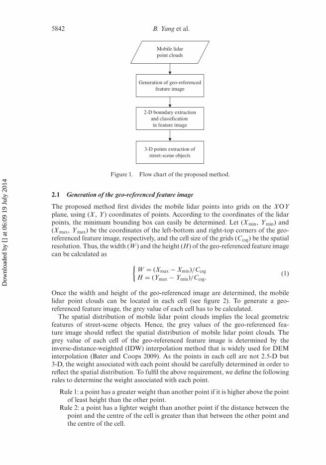
It is rather difficult to directly extract street-scene objects from mobile lidar pointclouds because of noise in the data, huge data volume and no explicit or ancillarydata (e.g. intensity image). Although clustering-based methods (Biosca and Lerma2008) can extract 3-D boundaries and local geometric features of street-scene objects,the efficiency is relatively low and the results are uncertain. We propose a methodfor generating a geo-referenced feature image that is capable of maintaining implicitgeometric features in mobile lidar point clouds. Hence, the existing operators forextracting line or key point features from imagery can be adopted to extract theboundaries of street-scene objects from the feature image generated. Figure 1 elabo-rates the flow chart of the proposed method. The proposed method encompasses twokey components, namely feature image generation and street-scene object extraction.
In light of the flow chart of the proposed method, feature image generation is thefirst step in street-scene object extraction. Although the geo-referenced feature imagecan preserve the spatial distribution and the density of mobile lidar points, the fea-ture image is also able to reflect the varied characteristics of different street-sceneobjects, which are represented as grey values in the feature image. To fulfil the aboverequirements, the grey values of each pixel and the resolution of the geo-referencedfeature image have to be determined.
Dow
nloa
ded
by [
] at
06:
09 1
9 Ju
ly 2
014
5842 B. Yang et al.
Mobile lidarpoint clouds
Generation of geo-referencedfeature image
2-D boundary extractionand classification in feature image
3-D points extraction ofstreet-scene objects
Figure 1. Flow chart of the proposed method.
2.1 Generation of the geo-referenced feature image
The proposed method first divides the mobile lidar points into grids on the XOYplane, using (X , Y ) coordinates of points. According to the coordinates of the lidarpoints, the minimum bounding box can easily be determined. Let (Xmin, Y min) and(Xmax, Y max) be the coordinates of the left-bottom and right-top corners of the geo-referenced feature image, respectively, and the cell size of the grids (Ccsg) be the spatialresolution. Thus, the width (W ) and the height (H) of the geo-referenced feature imagecan be calculated as
{W = (Xmax − Xmin)/Ccsg
H = (Ymax − Ymin)/Ccsg.(1)
Once the width and height of the geo-referenced image are determined, the mobilelidar point clouds can be located in each cell (see figure 2). To generate a geo-referenced feature image, the grey value of each cell has to be calculated.
The spatial distribution of mobile lidar point clouds implies the local geometricfeatures of street-scene objects. Hence, the grey values of the geo-referenced fea-ture image should reflect the spatial distribution of mobile lidar point clouds. Thegrey value of each cell of the geo-referenced feature image is determined by theinverse-distance-weighted (IDW) interpolation method that is widely used for DEMinterpolation (Bater and Coops 2009). As the points in each cell are not 2.5-D but3-D, the weight associated with each point should be carefully determined in order toreflect the spatial distribution. To fulfil the above requirement, we define the followingrules to determine the weight associated with each point.
Rule 1: a point has a greater weight than another point if it is higher above the pointof least height than the other point.
Rule 2: a point has a lighter weight than another point if the distance between thepoint and the centre of the cell is greater than that between the other point andthe centre of the cell.
Dow
nloa
ded
by [
] at
06:
09 1
9 Ju
ly 2
014

Object extraction from mobile lidar data 5843
Figure 2. Sketch map of cells and data points.
These two rules indicate that the weight of each point is determined by two factors,namely planar distance and height difference. Once the weight of each point is deter-mined, the grey value of each cell is calculated by the IDW interpolation method asfollows:
Fij =( nij∑
k=1
WijkZijk
)/( nij∑k=1
Wijk
), (2)
where Fij is the weighted average of the feature value of the cell with coordinates(i, j), which will be displayed as grey values in the image, nij is the number of scan-ning points in the cell, Wijk and Zijk are the weight and height of the kth point in thiscell (0 < k < nij), respectively, and the weight, Wijk, can be calculated by
Wijk = αW XYijk + βW H
ijk, (3)
where α and β are the coefficients of weights, which need to be tuned, W XYijk is the
weight of the kth point in the cell, calculated using only the planar distance in the cell,and W H
ijk is the weight of the kth point in the cell, calculated using only the heightdifference in the cell. They can be determined as follows:
⎧⎪⎨⎪⎩
W XYijk = √
2Ccsg
/(Dk
ij + δ)
W Hijk = Hk
ij (hmin(ij) − Zmin)/(Zmax − hmax(ij) + δ)
α + β = 1.0
, (4)
where Dkij is the planar distance from the kth point in the cell with coordinates
(i, j) to the centre of the cell, Hkij is the height difference from the kth point in the
Dow
nloa
ded
by [
] at
06:
09 1
9 Ju
ly 2
014
5844 B. Yang et al.
cell to the lowest point of the cell, hmin(ij) and hmax(ij) are the lowest and highestelevations in the cell, respectively, Zmax and Zmin are the lowest and highest ele-vations in the whole scanning area, respectively, and δ is a positive infinitesimalvalue to make the denominator of the equation be nonzero. The weight W H
ijk ofthe point calculated by the formula mentioned earlier is to emphasize high-lyingobjects and objects with a large standard deviation of height values. Dk
ij and Hkij are
calculated by
⎧⎨⎩Dk
ij =√(
xkij − xij
0
)2 +(
ykij − yij
0
)2
Hkij = Zijk − hmin(ij)
, (5)
where (xijk, yij
k) are the coordinates of the kth point in the cell with coordinates (i, j)and (xij
0 , yij0 ) are the coordinates of the centre of the cell.
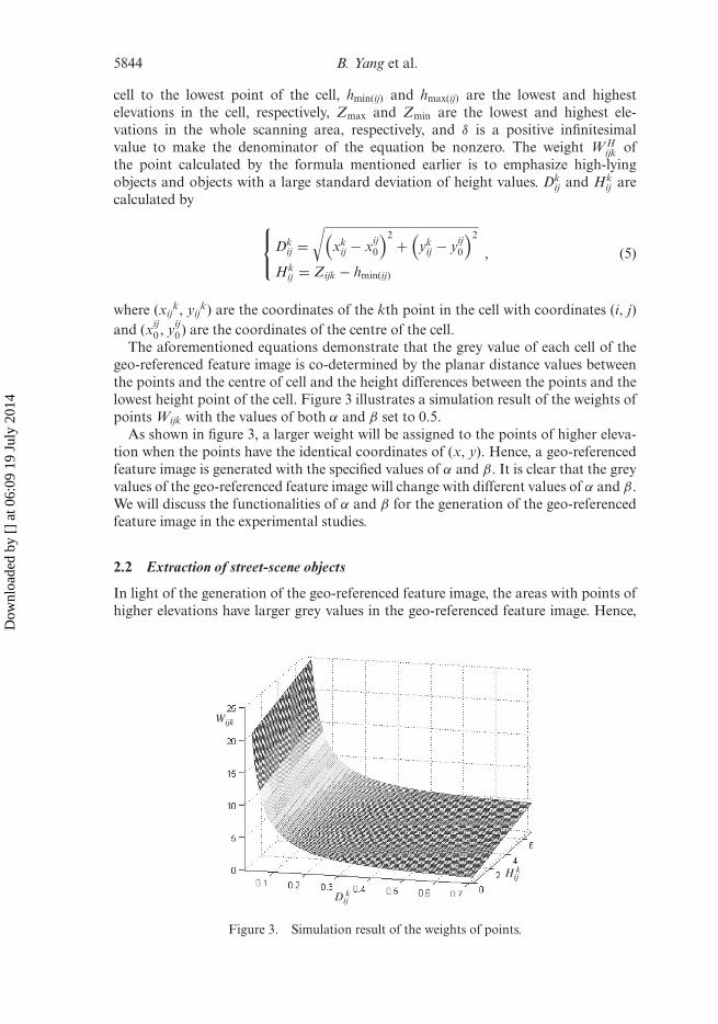
The aforementioned equations demonstrate that the grey value of each cell of thegeo-referenced feature image is co-determined by the planar distance values betweenthe points and the centre of cell and the height differences between the points and thelowest height point of the cell. Figure 3 illustrates a simulation result of the weights ofpoints Wijk with the values of both α and β set to 0.5.
As shown in figure 3, a larger weight will be assigned to the points of higher eleva-tion when the points have the identical coordinates of (x, y). Hence, a geo-referencedfeature image is generated with the specified values of α and β. It is clear that the greyvalues of the geo-referenced feature image will change with different values of α and β.We will discuss the functionalities of α and β for the generation of the geo-referencedfeature image in the experimental studies.
2.2 Extraction of street-scene objects
In light of the generation of the geo-referenced feature image, the areas with points ofhigher elevations have larger grey values in the geo-referenced feature image. Hence,
Wijk
Dijk
Hijk
Figure 3. Simulation result of the weights of points.
Dow
nloa
ded
by [
] at
06:
09 1
9 Ju
ly 2
014
Object extraction from mobile lidar data 5845
the areas of buildings and trees have larger grey values compared with their neigh-bouring areas (e.g. ground and roads). A threshold of grey value can be specified toextract the areas of larger grey values according to the histogram analysis on the geo-referenced feature image. In this study, we selected the method of discrete discriminantanalysis (Goldstein and Dillon 1978) to automatically specify the threshold because ofits robustness. The method of discrete discriminant analysis first finds the maximumand minimum grey values of the feature image. Then, it calculates the between-clustervariance under an assumed threshold. Finally, it finds the threshold with the highestvalue of between-cluster variances as the optimal threshold, which is used to classifythe pixels into different categories.
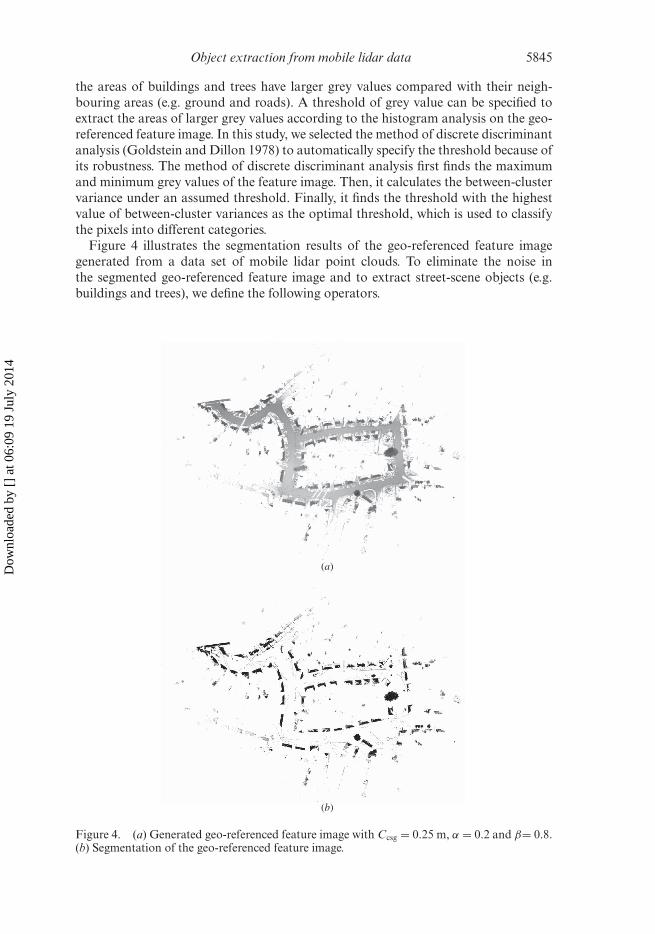
Figure 4 illustrates the segmentation results of the geo-referenced feature imagegenerated from a data set of mobile lidar point clouds. To eliminate the noise inthe segmented geo-referenced feature image and to extract street-scene objects (e.g.buildings and trees), we define the following operators.
(a)
(b)
Figure 4. (a) Generated geo-referenced feature image with Ccsg = 0.25 m, α = 0.2 and β= 0.8.(b) Segmentation of the geo-referenced feature image.
Dow
nloa
ded
by [
] at
06:
09 1
9 Ju
ly 2
014
5846 B. Yang et al.
2.2.1 Boundary extraction. In the field of image processing, many methods havebeen proposed to extract contours in 2-D image space, including the most widely usedCanny edge detector (Canny 1986) and the active contour model (Kass et al. 1988).As we deal with a segmented binary feature image (the background is black) here, weimplement contour extraction in a simple way. A pixel is changed into white if it is ablack pixel and its eight neighbouring pixels are black as well. In this way, the blackpixels whose eight neighbouring pixels are not all black will be labelled as boundarypixels.
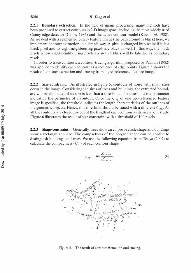
In order to trace contours, a contour-tracing algorithm proposed by Pavlidis (1982)was applied to identify each contour as a sequence of edge points. Figure 5 shows theresult of contour extraction and tracing from a geo-referenced feature image.
2.2.2 Size constraint. As illustrated in figure 5, contours of noise with small sizesoccur in the image. Considering the sizes of trees and buildings, the extracted bound-ary will be eliminated if its size is less than a threshold. The threshold is a parameterindicating the perimeter of a contour. Once the Ccsg of one geo-referenced featureimage is specified, the threshold indicates the length characteristics of the outlines ofthe geometric objects. Hence, this threshold should be tuned with a different Ccsg. Asall the contours are closed, we count the length of each contour as its size in our study.Figure 6 illustrates the result of size constraint with a threshold of 100 pixels.
2.2.3 Shape constraint. Generally, trees show an ellipse or circle shape and buildingsshow a rectangular shape. The compactness of the polygon shape can be applied todistinguish buildings and trees. We use the following equation from Touya (2007) tocalculate the compactness (Csp) of each contour shape.
Csp = 4πScontour
P2contour
, (6)
Figure 5. The result of contour extraction and tracing.
Dow
nloa
ded
by [
] at
06:
09 1
9 Ju
ly 2
014
Object extraction from mobile lidar data 5847
Figure 6. Filtering shapes by size constraint (threshold = 100 pixels).
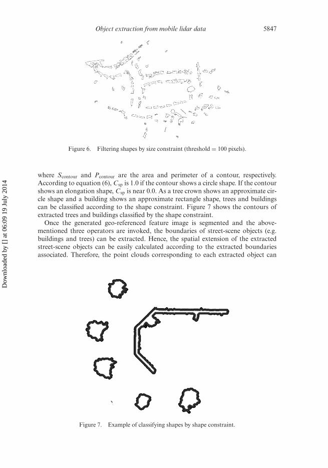
where Scontour and Pcontour are the area and perimeter of a contour, respectively.According to equation (6), Csp is 1.0 if the contour shows a circle shape. If the contourshows an elongation shape, Csp is near 0.0. As a tree crown shows an approximate cir-cle shape and a building shows an approximate rectangle shape, trees and buildingscan be classified according to the shape constraint. Figure 7 shows the contours ofextracted trees and buildings classified by the shape constraint.
Once the generated geo-referenced feature image is segmented and the above-mentioned three operators are invoked, the boundaries of street-scene objects (e.g.buildings and trees) can be extracted. Hence, the spatial extension of the extractedstreet-scene objects can be easily calculated according to the extracted boundariesassociated. Therefore, the point clouds corresponding to each extracted object can
Figure 7. Example of classifying shapes by shape constraint.
Dow
nloa
ded
by [
] at
06:
09 1
9 Ju
ly 2
014
5848 B. Yang et al.
be extracted from the mobile lidar point clouds according to the spatial extensioncalculated.
Generally, the perimeter of a tree crown is larger compared with that of the treetrunk. The perimeters of buildings at different heights are usually kept at a constantvalue. In addition, the mean perimeter of a building in the Z direction is usually muchlarger than that of a tree. Hence, buildings and trees show different profiles in the Zdirection, and this can be used to further classify buildings and trees from point clouds.
Given an unknown object with points, the area of a profile at a specified height (Ap)can be calculated with all the points lying in profile in the Z direction. These areas ofprofiles at different heights are used to compute the mean value (μA) of profile areasin the Z direction. Therefore, a threshold of μA can be set to distinguish buildings andtrees. If μA is smaller than the specified threshold, this object will be classified as trees.Otherwise, this object will be considered a building.
3. Experimental studies
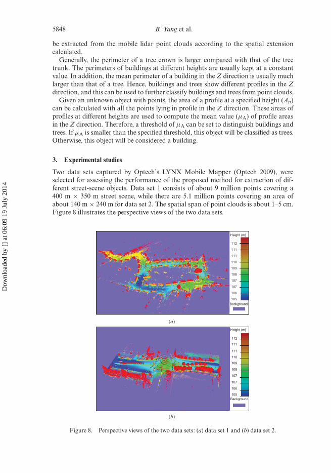
Two data sets captured by Optech’s LYNX Mobile Mapper (Optech 2009), wereselected for assessing the performance of the proposed method for extraction of dif-ferent street-scene objects. Data set 1 consists of about 9 million points covering a400 m × 350 m street scene, while there are 5.1 million points covering an area ofabout 140 m × 240 m for data set 2. The spatial span of point clouds is about 1–5 cm.Figure 8 illustrates the perspective views of the two data sets.
(a)
Height (m)
112
112
111
111
111
111
110
109
108
107
107
106
105
110
109
108
107
107
106
105Background
Height (m)
Background
(b)
Figure 8. Perspective views of the two data sets: (a) data set 1 and (b) data set 2.
Dow
nloa
ded
by [
] at
06:
09 1
9 Ju
ly 2
014
Object extraction from mobile lidar data 5849
3.1 Geo-referenced feature image generation
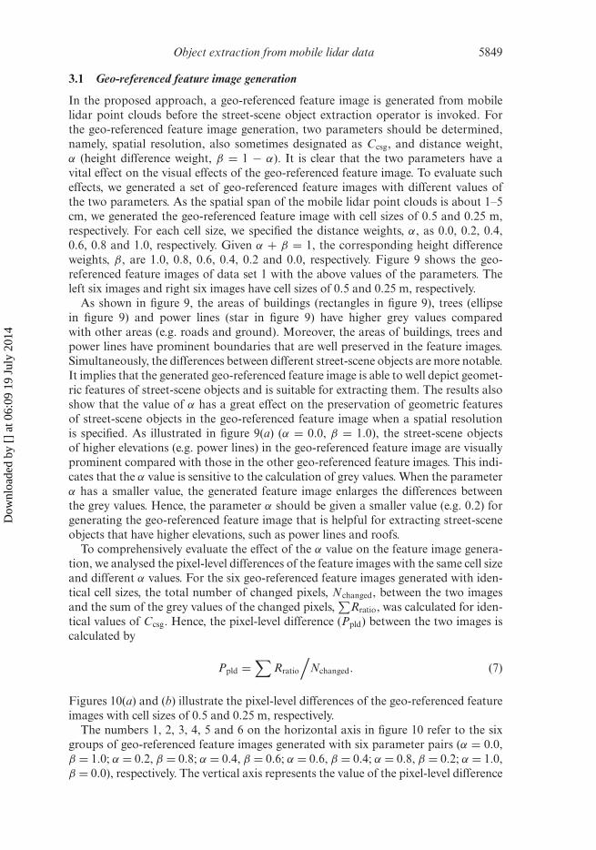
In the proposed approach, a geo-referenced feature image is generated from mobilelidar point clouds before the street-scene object extraction operator is invoked. Forthe geo-referenced feature image generation, two parameters should be determined,namely, spatial resolution, also sometimes designated as Ccsg, and distance weight,α (height difference weight, β = 1 − α). It is clear that the two parameters have avital effect on the visual effects of the geo-referenced feature image. To evaluate sucheffects, we generated a set of geo-referenced feature images with different values ofthe two parameters. As the spatial span of the mobile lidar point clouds is about 1–5cm, we generated the geo-referenced feature image with cell sizes of 0.5 and 0.25 m,respectively. For each cell size, we specified the distance weights, α, as 0.0, 0.2, 0.4,0.6, 0.8 and 1.0, respectively. Given α + β = 1, the corresponding height differenceweights, β, are 1.0, 0.8, 0.6, 0.4, 0.2 and 0.0, respectively. Figure 9 shows the geo-referenced feature images of data set 1 with the above values of the parameters. Theleft six images and right six images have cell sizes of 0.5 and 0.25 m, respectively.
As shown in figure 9, the areas of buildings (rectangles in figure 9), trees (ellipsein figure 9) and power lines (star in figure 9) have higher grey values comparedwith other areas (e.g. roads and ground). Moreover, the areas of buildings, trees andpower lines have prominent boundaries that are well preserved in the feature images.Simultaneously, the differences between different street-scene objects are more notable.It implies that the generated geo-referenced feature image is able to well depict geomet-ric features of street-scene objects and is suitable for extracting them. The results alsoshow that the value of α has a great effect on the preservation of geometric featuresof street-scene objects in the geo-referenced feature image when a spatial resolutionis specified. As illustrated in figure 9(a) (α = 0.0, β = 1.0), the street-scene objectsof higher elevations (e.g. power lines) in the geo-referenced feature image are visuallyprominent compared with those in the other geo-referenced feature images. This indi-cates that the α value is sensitive to the calculation of grey values. When the parameterα has a smaller value, the generated feature image enlarges the differences betweenthe grey values. Hence, the parameter α should be given a smaller value (e.g. 0.2) forgenerating the geo-referenced feature image that is helpful for extracting street-sceneobjects that have higher elevations, such as power lines and roofs.
To comprehensively evaluate the effect of the α value on the feature image genera-tion, we analysed the pixel-level differences of the feature images with the same cell sizeand different α values. For the six geo-referenced feature images generated with iden-tical cell sizes, the total number of changed pixels, Nchanged, between the two imagesand the sum of the grey values of the changed pixels,
∑Rratio, was calculated for iden-
tical values of Ccsg. Hence, the pixel-level difference (Ppld) between the two images iscalculated by
Ppld =∑
Rratio
/Nchanged. (7)
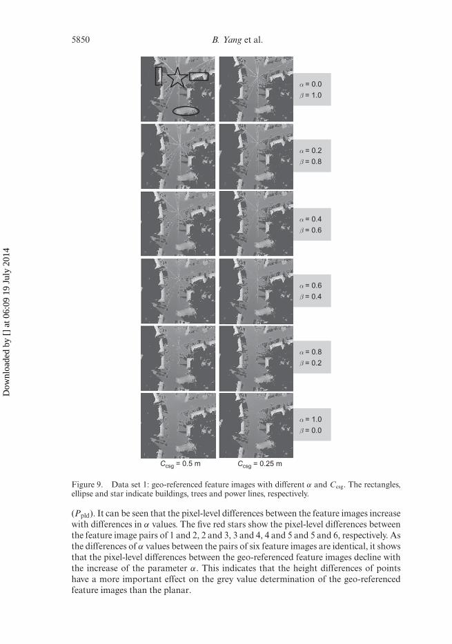
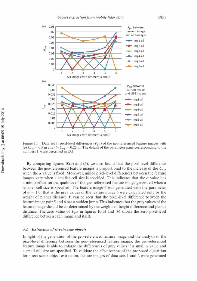
Figures 10(a) and (b) illustrate the pixel-level differences of the geo-referenced featureimages with cell sizes of 0.5 and 0.25 m, respectively.
The numbers 1, 2, 3, 4, 5 and 6 on the horizontal axis in figure 10 refer to the sixgroups of geo-referenced feature images generated with six parameter pairs (α = 0.0,β = 1.0; α = 0.2, β = 0.8; α = 0.4, β = 0.6; α = 0.6, β = 0.4; α = 0.8, β = 0.2; α = 1.0,β = 0.0), respectively. The vertical axis represents the value of the pixel-level difference
Dow
nloa
ded
by [
] at
06:
09 1
9 Ju
ly 2
014
5850 B. Yang et al.
α = 0.0
β = 1.0
α = 0.2
β = 0.8
α = 0.4
β = 0.6
α = 0.6
β = 0.4
α = 0.8
β = 0.2
α = 1.0
β = 0.0
Ccsg = 0.5 m Ccsg = 0.25 m
Figure 9. Data set 1: geo-referenced feature images with different α and Ccsg. The rectangles,ellipse and star indicate buildings, trees and power lines, respectively.
(Ppld). It can be seen that the pixel-level differences between the feature images increasewith differences in α values. The five red stars show the pixel-level differences betweenthe feature image pairs of 1 and 2, 2 and 3, 3 and 4, 4 and 5 and 5 and 6, respectively. Asthe differences of α values between the pairs of six feature images are identical, it showsthat the pixel-level differences between the geo-referenced feature images decline withthe increase of the parameter α. This indicates that the height differences of pointshave a more important effect on the grey value determination of the geo-referencedfeature images than the planar.
Dow
nloa
ded
by [
] at
06:
09 1
9 Ju
ly 2
014
Object extraction from mobile lidar data 5851
0
0.01
0.02
0.03
0.04
0.05
0.06
0.07
0.08 Ppld
between
current image
and all 6 images
Ppld
between
current image
and all 6 images
Pp
ld
Img1-all
Img2-all
Img3-all
Img4-all
Img5-all
Img6-all
Img1-all
Img2-all
Img3-all
Img4-all
Img5-all
Img6-all
0
0.005
0.01
0.015
0.02
0.025
0.03
0.035
0.04
0.045
2 3
Six images with different α and β
Six images with different α and β
4 51 6
2 3 4 51 6
Pp
ld
(a)
(b)
Figure 10. Data set 1: pixel-level differences (Ppld) of the geo-referenced feature images with(a) Ccsg = 0.5 m and (b) Ccsg = 0.25 m. The details of the parameter pairs corresponding to thenumbers 1–6 are described in §3.1.
By comparing figures 10(a) and (b), we also found that the pixel-level differencebetween the geo-referenced feature images is proportional to the increase of the Ccsg
when the α value is fixed. Moreover, minor pixel-level differences between the featureimages vary when a smaller cell size is specified. This indicates that the α value hasa minor effect on the qualities of the geo-referenced feature image generated when asmaller cell size is specified. The feature image 6 was generated with the parameterof α = 1.0, that is the grey values of the feature image 6 were calculated only by theweight of planar distance. It can be seen that the pixel-level difference between thefeature image pair 5 and 6 has a sudden jump. This indicates that the grey values of thefeature image should be co-determined by the weights of height difference and planardistance. The zero value of Ppld in figures 10(a) and (b) shows the zero pixel-leveldifference between each image and itself.
3.2 Extraction of street-scene objects
In light of the generation of the geo-referenced feature image and the analysis of thepixel-level difference between the geo-referenced feature images, the geo-referencedfeature image is able to enlarge the differences of grey values if a small α value anda small cell size are specified. To validate the effectiveness of the proposed algorithmfor street-scene object extraction, feature images of data sets 1 and 2 were generated
Dow
nloa
ded
by [
] at
06:
09 1
9 Ju
ly 2
014
5852 B. Yang et al.
with the parameters of α = 0.2, β = 0.8 and Ccsg = 0.25 m. This configuration ofparameters is beneficial for emphasizing high-lying objects.
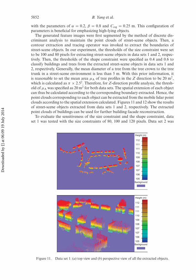
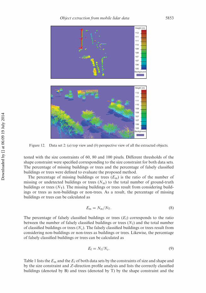
The generated feature images were first segmented by the method of discrete dis-criminant analysis to maintain the point clouds of street-scene objects. Then, acontour extraction and tracing operator was invoked to extract the boundaries ofstreet-scene objects. In our experiment, the thresholds of the size constraint were setto be 100 and 80 pixels for extracting street-scene objects in data sets 1 and 2, respec-tively. Then, the thresholds of the shape constraint were specified as 0.4 and 0.6 toclassify buildings and trees from the extracted street-scene objects in data sets 1 and2, respectively. Generally, the mean diameter of a tree from the tree crown to the treetrunk in a street-scene environment is less than 5 m. With this prior information, itis reasonable to set the mean area μA of tree profiles in the Z direction to be 20 m2,which is calculated as π × 2.52. Therefore, for Z-direction profile analysis, the thresh-old of μA was specified as 20 m2 for both data sets. The spatial extension of each objectcan thus be calculated according to the corresponding boundary extracted. Hence, thepoint clouds corresponding to each object can be extracted from the mobile lidar pointclouds according to the spatial extension calculated. Figures 11 and 12 show the resultsof street-scene objects extracted from data sets 1 and 2, respectively. The extractedpoint clouds of buildings can be used for further building facade reconstruction.
To evaluate the sensitiveness of the size constraint and the shape constraint, dataset 1 was tested with the size constraints of 80, 100 and 120 pixels. Data set 2 was
Height (m)
112
112
111
111
111
111
110
109
108
107
107
106
105
110
109
108
107
107
106
105Background
Height (m)
Background
Figure 11. Data set 1: (a) top view and (b) perspective view of all the extracted objects.
Dow
nloa
ded
by [
] at
06:
09 1
9 Ju
ly 2
014
Object extraction from mobile lidar data 5853
Height (m)
112
112
111
111
111
111
110
109
108
107
107
106
105
110
109
108
107
107
106
105
Background
Height (m)
Background
Figure 12. Data set 2: (a) top view and (b) perspective view of all the extracted objects.
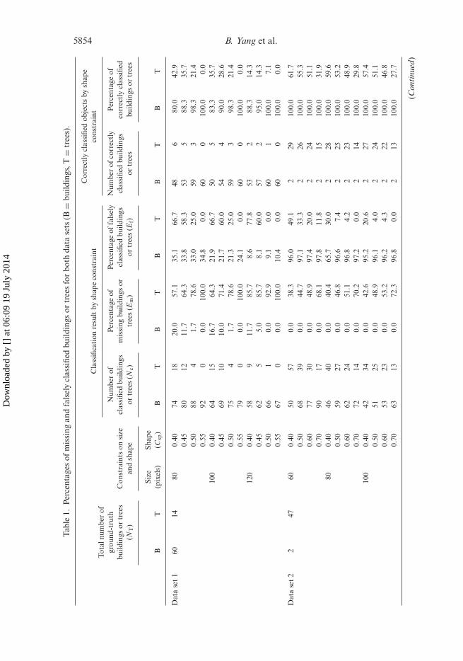
tested with the size constraints of 60, 80 and 100 pixels. Different thresholds of theshape constraint were specified corresponding to the size constraint for both data sets.The percentage of missing buildings or trees and the percentage of falsely classifiedbuildings or trees were defined to evaluate the proposed method.
The percentage of missing buildings or trees (Em) is the ratio of the number ofmissing or undetected buildings or trees (Nm) to the total number of ground-truthbuildings or trees (NT). The missing buildings or trees result from considering build-ings or trees as non-buildings or non-trees. As a result, the percentage of missingbuildings or trees can be calculated as
Em = Nm/NT. (8)
The percentage of falsely classified buildings or trees (Ef) corresponds to the ratiobetween the number of falsely classified buildings or trees (Nf) and the total numberof classified buildings or trees (Nc). The falsely classified buildings or trees result fromconsidering non-buildings or non-trees as buildings or trees. Likewise, the percentageof falsely classified buildings or trees can be calculated as
Ef = Nf/Nc. (9)
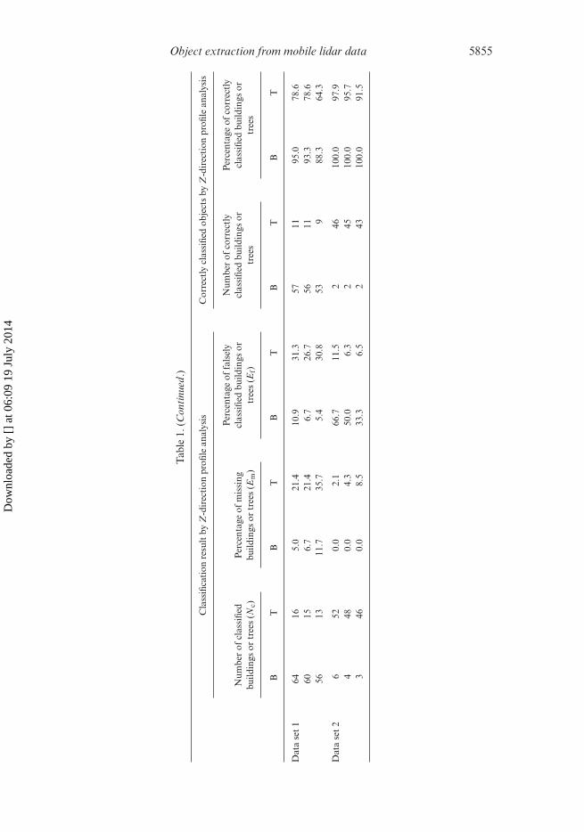
Table 1 lists the Em and the Ef of both data sets by the constraints of size and shape andby the size constraint and Z-direction profile analysis and lists the correctly classifiedbuildings (denoted by B) and trees (denoted by T) by the shape constraint and the
Dow
nloa
ded
by [
] at
06:
09 1
9 Ju
ly 2
014
5854 B. Yang et al.
Tab
le1.
Per
cent
ages
ofm
issi
ngan
dfa
lsel
ycl
assi
fied
build
ings
ortr
ees
for
both
data
sets
(B=
build
ings
,T=
tree
s).
Cla
ssifi
cati
onre
sult
bysh
ape
cons
trai
ntC
orre
ctly
clas
sifie
dob
ject
sby
shap
eco
nstr
aint
Tota
lnum
ber
ofgr
ound
-tru
thbu
ildin
gsor
tree
s(N
T)
Con
stra
ints
onsi
zean
dsh
ape
Num
ber
ofcl
assi
fied
build
ings
ortr
ees
(Nc)
Per
cent
age
ofm
issi
ngbu
ildin
gsor
tree
s(E
m)
Per
cent
age
offa
lsel
ycl
assi
fied
build
ings
ortr
ees
(Ef)
Num
ber
ofco
rrec
tly
clas
sifie
dbu
ildin
gsor
tree
s
Per
cent
age
ofco
rrec
tly
clas
sifie
dbu
ildin
gsor
tree
s
BT
Size
(pix
els)
Shap
e(C
sp)
BT
BT
BT
BT
BT
Dat
ase
t1
6014
800.
4074
1820
.057
.135
.166
.748
680
.042
.90.
4580
1211
.764
.333
.858
.353
588
.335
.70.
5088
41.
778
.633
.025
.059
398
.321
.40.
5592
00.
010
0.0
34.8
0.0
600
100.
00.
010
00.
4064
1516
.764
.321
.966
.750
583
.335
.70.
4569
1010
.071
.421
.760
.054
490
.028
.60.
5075
41.
778
.621
.325
.059
398
.321
.40.
5579
00.
010
0.0
24.1
0.0
600
100.
00.
012
00.
4058
911
.785
.78.
677
.853
288
.314
.30.
4562
55.
085
.78.
160
.057
295
.014
.30.
5066
10.
092
.99.
10.
060
110
0.0
7.1
0.55
670
0.0
100.
010
.40.
060
010
0.0
0.0
Dat
ase
t2
247
600.
4050
570.
038
.396
.049
.12
2910
0.0
61.7
0.50
6839
0.0
44.7
97.1
33.3
226
100.
055
.30.
6077
300.
048
.997
.420
.02
2410
0.0
51.1
0.70
9017
0.0
68.1
97.8
11.8
215
100.
031
.980
0.40
4640
0.0
40.4
65.7
30.0
228
100.
059
.60.
5059
270.
046
.896
.67.
42
2510
0.0
53.2
0.60
6224
0.0
51.1
96.8
4.2
223
100.
048
.90.
7072
140.
070
.297
.20.
02
1410
0.0
29.8
100
0.40
4234
0.0
42.6
95.2
20.6
227
100.
057
.40.
5051
250.
048
.996
.14.
02
2410
0.0
51.1
0.60
5323
0.0
53.2
96.2
4.3
222
100.
046
.80.
7063
130.
072
.396
.80.
02
1310
0.0
27.7
(Con
tinu
ed)
Dow
nloa
ded
by [
] at
06:
09 1
9 Ju
ly 2
014
Object extraction from mobile lidar data 5855
Tab
le1.
(Con
tinu
ed.)
Cla
ssifi
cati
onre
sult
byZ
-dir
ecti
onpr
ofile
anal
ysis
Cor
rect
lycl
assi
fied
obje
cts
byZ
-dir
ecti
onpr
ofile
anal
ysis
Num
ber
ofcl
assi
fied
build
ings
ortr
ees
(Nc)
Per
cent
age
ofm
issi
ngbu
ildin
gsor
tree
s(E
m)
Per
cent
age
offa
lsel
ycl
assi
fied
build
ings
ortr
ees
(Ef)
Num
ber
ofco
rrec
tly
clas
sifie
dbu
ildin
gsor
tree
s
Per
cent
age
ofco
rrec
tly
clas
sifie
dbu
ildin
gsor
tree
s
BT
BT
BT
BT
BT
Dat
ase
t1
6416
5.0
21.4
10.9
31.3
5711
95.0
78.6
6015
6.7
21.4
6.7
26.7
5611
93.3
78.6
5613
11.7
35.7
5.4
30.8
539
88.3
64.3
Dat
ase
t2
652
0.0
2.1
66.7
11.5
246
100.
097
.94
480.
04.
350
.06.
32
4510
0.0
95.7
346
0.0
8.5
33.3
6.5
243
100.
091
.5
Dow
nloa
ded
by [
] at
06:
09 1
9 Ju
ly 2
014
5856 B. Yang et al.
Z-direction profile analysis. The total number of ground-truth buildings (NTb) andtrees (NTt) were manually counted for both data sets. It can be seen that data set1 contains more buildings (60 buildings and 14 trees) and data set 2 contains moretrees (2 buildings and 47 trees). As listed in table 1, the Em and the Ef of data sets1 and 2 were high when only the size and the shape of constraints were used. It canbe seen that the threshold of the shape constraint has a large effect on the Em andthe Ef. The percentages of missing buildings (Emb) and falsely classified trees (Eft)decline with the increase of the threshold of the shape constraint according to theshape constraint. However, the percentages of missing trees (Emt) and falsely classifiedbuildings (Efb) show the opposite trend. This dilemma leads to difficulties in specifyingthe threshold of the shape constraint. The percentage of missing trees (Emt) in data set2 is 70.2% with a shape constraint of 0.7 and a size constraint of 80 pixels. This isbecause many trees and buildings have almost the same outlines, especially when thetrees are dense. However, the results were substantially improved when an additionalZ-direction profile analysis was used. It can be seen that the percentage of missing trees(Emt) using Z-direction profile analysis increases with the increase of the threshold ofthe size constraint, while the percentage of falsely classified buildings (Efb) declines.As the threshold of μA is related to the spatial extension of an object, the percentagesof missing buildings and falsely classified trees will be higher with a larger thresholdof μA. The larger the threshold of μA that is specified, the more buildings will beclassified as trees, which leads to the increase of the percentages of missing buildingsand falsely classified trees.
3.3 Comparison with DoPP algorithm and FCM clustering
To demonstrate the efficiency and effectiveness of the proposed algorithm imple-mented in C++ language, the DoPP algorithm and the fuzzy C-means (FCM)clustering (Biosca and Lerma 2008) were compared in our experiment.
The DoPP algorithm divides the mobile lidar points into cells with a certain sizein the XOY plane. Then, the threshold of the minimum number of points in onecell is specified for finding those cells which have the number of points more thanthe specified threshold. The points located in those cells are considered to belong tobuilding facade points. The FCM clustering method (Biosca and Lerma 2008) con-sists of two steps, namely the classification of data points into surface categories andthe classification of points lying on planar features into different planes accordingto the feature vector, which was calculated by the distance from a point to its best-fitting plane along its normal direction. In our study, the feature vector of a pointwas used to classify the point clouds into planar surfaces, undulating surfaces and therest.
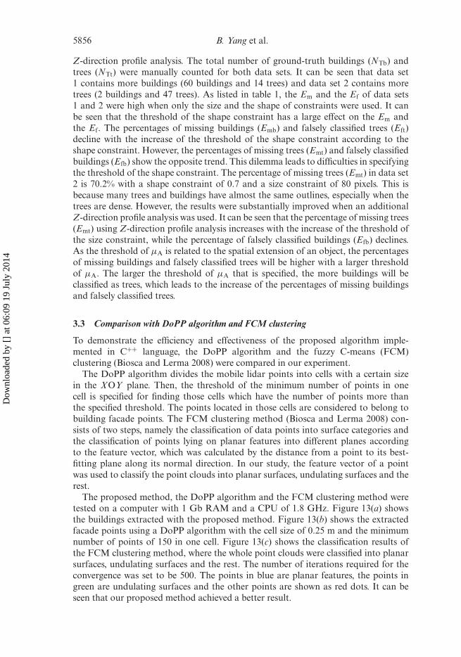
The proposed method, the DoPP algorithm and the FCM clustering method weretested on a computer with 1 Gb RAM and a CPU of 1.8 GHz. Figure 13(a) showsthe buildings extracted with the proposed method. Figure 13(b) shows the extractedfacade points using a DoPP algorithm with the cell size of 0.25 m and the minimumnumber of points of 150 in one cell. Figure 13(c) shows the classification results ofthe FCM clustering method, where the whole point clouds were classified into planarsurfaces, undulating surfaces and the rest. The number of iterations required for theconvergence was set to be 500. The points in blue are planar features, the points ingreen are undulating surfaces and the other points are shown as red dots. It can beseen that our proposed method achieved a better result.
Dow
nloa
ded
by [
] at
06:
09 1
9 Ju
ly 2
014
Object extraction from mobile lidar data 5857
Figure 13. Object extraction by (a) the proposed method, (b) the DoPP algorithm and (c)FCM clustering.
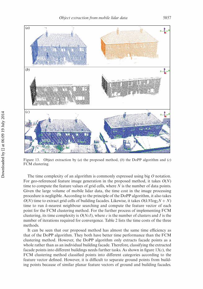
The time complexity of an algorithm is commonly expressed using big O notation.For geo-referenced feature image generation in the proposed method, it takes O(N)time to compute the feature values of grid cells, where N is the number of data points.Given the large volume of mobile lidar data, the time cost in the image processingprocedure is negligible. According to the principle of the DoPP algorithm, it also takesO(N) time to extract grid cells of building facades. Likewise, it takes O(kNlog2N + N)time to run k-nearest neighbour searching and compute the feature vector of eachpoint for the FCM clustering method. For the further process of implementing FCMclustering, its time complexity is O(NcI), where c is the number of clusters and I is thenumber of iterations required for convergence. Table 2 lists the time costs of the threemethods.
It can be seen that our proposed method has almost the same time efficiency asthat of the DoPP algorithm. They both have better time performance than the FCMclustering method. However, the DoPP algorithm only extracts facade points as awhole rather than as an individual building facade. Therefore, classifying the extractedfacade points into different buildings needs further tasks. As shown in figure 13(c), theFCM clustering method classified points into different categories according to thefeature vector defined. However, it is difficult to separate ground points from build-ing points because of similar planar feature vectors of ground and building facades.
Dow
nloa
ded
by [
] at
06:
09 1
9 Ju
ly 2
014
5858 B. Yang et al.
Table 2. Time efficiency comparison of the three methods.
Method Procedure (Ccsg = 0.25 m) Processing time (s)
DoPP algorithm Counting points in grids 2.095Building facade extraction 26.140
FCM clustering Feature vector calculation of each point 1823.52Classification of all points using FCM 609.66
The proposed method Generation of feature image 3.7012-D object classification 0.1403-D street-scene object extraction 24.180
Note: DoPP, density of projected points; FCM, fuzzy C-means.
Our proposed method is capable of classifying the extracted points into differentobjects (e.g. buildings). It also demonstrates that the proposed method maintainsthe local geometric features of street-scene objects. For instance, the point clouds ofbuilding roofs and tree crowns are well preserved in the extracted point clouds,which is particularly useful for further building facade reconstruction with high levelsof detail.
4. Discussion
The extraction of street-scene objects from mobile lidar point clouds is quite a time-consuming job due to huge data volumes and a lack of explicit geometric features.This article proposes a promising solution for efficiently extracting point clouds ofstreet-scene objects from mobile lidar point clouds. The main contributions of theproposed method are the generation of the geo-referenced feature image first fol-lowed by extracting street-scene objects from the feature image. Thus, the proposedmethod transforms the extraction of street-scene objects from 3-D point clouds toobject extraction from 2-D imagery. We have presented a formula to calculate the greyvalues of the geo-referenced feature image with a specified cell size of the grid (e.g. 25cm). Image segmentation and contour extraction techniques were applied to extractthe boundaries of street-scene objects in image space. Hence, the point clouds of thestreet-scene objects (e.g. buildings and trees) can be extracted in 3-D according to theboundaries associated.
The calculation of the grey values of the geo-referenced feature image demonstratesthat the generated feature image is of vital importance for efficiently extracting street-scene objects from mobile lidar point clouds. Moreover, two parameters, namely thecell size of the feature image and the weights of points, determine the qualities of thefeature images generated. The cell size of the grid can be obtained from the acquisi-tion parameters, such as the scanning frequency and average span between the scannedpoints. The weights of points of each cell consist of height differences with the mini-mum height of the whole area and the planar distances to the centre of the cell. Theanalysis of pixel-level differences between the generated feature images shows that theheight differences of points play a more important role for the weights of points com-pared with the planar distance values. That is why we assign a larger proportion tothe height differences part for the determination of the weights of points. This is alsohelpful for enlarging the grey-value differences of the geo-referenced feature image,which is useful for extracting the boundaries of high-lying street-scene objects. On theother hand, an α value is easily tuned to generate the geo-referenced feature images
Dow
nloa
ded
by [
] at
06:
09 1
9 Ju
ly 2
014
Object extraction from mobile lidar data 5859
with a given cell size for different purposes. For example, the geo-referenced featureimage can be generated with a low α value for enlarging the grey values of the areaof higher elevations, which is beneficial for the extraction of power lines, as shown infigure 9 (dotted in star).
In our method, the threshold of the size constraint differs from objects to beextracted and is affected by the cell size of grids. It may be difficult to automaticallyadjust the threshold of the size constraint for different street-scene objects withoutprior knowledge. On the other hand, the proposed method calculates the compactnessof each extracted object as a shape constraint to classify buildings and tree crowns.It can be seen that the shape constraint has a large effect on the two types of errors.Moreover, when compared with the size constraint, the shape constraint is more dif-ficult to specify. Hence, many non-trees and non-buildings were misclassified as treesand buildings. Nevertheless, the percentages of missing buildings or trees and falselyclassified buildings or trees were greatly reduced by 50% and 70%, respectively, withan additional Z-direction profile analysis. This is because the profiles of buildings andtrees in the Z-direction are different. With prior knowledge of the diameter of thetree crown, the threshold of the mean area of tree profiles was easily specified for theZ-direction profile analysis.
5. Conclusions
Automated extraction of street-scene objects from mobile lidar point clouds remainsa major unsolved problem in the use of mobile lidar mapping systems. A key issue isto identify geometric features (e.g. the boundary of a building) from 3-D lidar pointclouds. This article has presented a novel solution for efficiently extracting street-scene objects (e.g. buildings and trees) from point clouds collected by Optech’s LYNXMobile Mapping System. Our method consists of three key steps: (1) determination ofthe weights of points, (2) generation of a geo-referenced feature image and (3) imagesegmentation towards object extraction from the feature image. The geo-referencedfeature image generated from mobile lidar point clouds is able to represent the spatialdistribution of scanned points and preserve the local geometric features of street-sceneobjects. The experimental results demonstrate that our method is capable of generat-ing the geo-referenced feature image, in which the geometric features of street-sceneobjects are well preserved with the two parameters of the cell size and point weights.Moreover, these two parameters can easily be tuned for different purposes. In addi-tion, our method demonstrates high computational efficiency for the extraction ofpoint clouds of street-scene objects, which is beneficial for further reconstruction ofbuilding facades. Our further studies will focus on vector-based 3-D construction ofstreet-scene objects based on the point clouds of the extracted building.
AcknowledgementsThe work presented in this article was substantially supported by NSFC (No.41071268), the Outstanding Talented Project from the Ministry of Education ofPR China (NCET-07-0643) and the Fundamental Research Funds for the CentralUniversities (No. 3103005). The LYNX Mobile Mapper data sets were provided byOpech Inc. The authors thank the anonymous reviewers for their insightful commentsand suggestions.
Dow
nloa
ded
by [
] at
06:
09 1
9 Ju
ly 2
014
5860 B. Yang et al.
ReferencesABUHADROUS, I., AMMOUN, S., NASHASHIBI, F., GOULETTE, F. and LAURGEAU, C., 2004.
Digitizing and 3D modeling of urban environments and roads using vehicle-bornelaser scanner system. In Proceedings of 2004 IEEE/RSJ International Conference onIntelligent Robots and Systems (IROS 2004), 28 September–2 October 2004, Sendai,Japan (Piscataway, NJ: IEEE Press), vol. 1, pp. 76–81.
AKEL, N.A., FILIN, S. and DOVTSHER, Y., 2009, Reconstruction of complex shape build-ings from lidar data using free form surfaces. Photogrammetric Engineering & RemoteSensing, 75, pp. 271–280.
AXELSSON, P., 2000, DEM generation from laser scanner data using adaptive TIN models.International Archives of the Photogrammetry Remote Sensing and Spatial InformationSciences, 33, pp. 110–117.
BARBER, D., MILLS, J. and SMITH, V.S., 2008, Geometric validation of a ground-based mobilelaser scanning system. ISPRS Journal of Photogrammetry and Remote Sensing, 63,pp. 128–141.
BATER, C.W. and COOPS, N.C., 2009, Evaluating error associated with lidar-derived DEMinterpolation. Computers & Geosciences, 35, pp. 289–300.
BECKER, S., 2009, Generation and application of rules for quality dependent façade reconstruc-tion. ISPRS Journal of Photogrammetry and Remote Sensing, 64, pp. 640–653.
BECKER, S. and HAALA, N., 2007, Combined feature extraction for façade reconstruction. InProceedings of the ISPRS Workshop on Laser Scanning 2007 and SilviLaser 2007, 12–14 September 2007, P. Rönnholm, H. Hyyppä and J. Hyyppä (Eds.), Espoo, Finland(Laser Scanning 2007 and SilviLaser 2007 Organizing Committee (ISPRS)), pp. 44–49.
BIOSCA, J.M. and LERMA, J.L., 2008, Unsupervised robust planar segmentation of terres-trial laser scanner point clouds based on fuzzy clustering methods. ISPRS Journal ofPhotogrammetry & Remote Sensing, 63, pp. 84–98.
BROVELLI, M.A. and CANNATA, M., 2004, Digital terrain model reconstruction in urban areasfrom airborne laser scanning data: the method and the example of the town of Pavia(Northern Italy). Computers & Geosciences, 30, pp. 325–331.
CANNY, J.F., 1986, A computational approach to edge detection. IEEE Transactions on PatternAnalysis and Machine Intelligence, 8, pp. 679–698.
GOLDSTEIN, M. and DILLON, W.R., 1978, Discrete Discriminant Analysis (New York: Wiley).HAALA, N. and BRENNER, C., 1999, Extraction of buildings and trees in urban environments.
ISPRS Journal of Photogrammetry & Remote Sensing, 54, pp. 130–137.HAALA, N., PETER, M., CEFALU, A. and KREMER, J., 2008a, Mobile lidar mapping for
urban data capture. In VSMM 2008 – Conference on Virtual Systems and MultiMediaDedicated to Digital Heritage, 20–25 October 2008, D. Pitzalis (Ed.), Limassol, Cyprus(VSMM 2008 Organizing Committee), pp. 101–106.
HAALA, N., PETER, M., KREMER, J. and HUNTER, G., 2008b, Mobile lidar mapping for 3Dpoint cloud collection in urban areas – a performance test. International Archives ofPhotogrammetry, Remote Sensing and Spatial Information Sciences, 37, pp. 1119–1124.
HUNTER, G., COX, C. and KREMER, J., 2006, Development of a commercial laser scanningmobile mapping system – StreetMapper. In 2nd International Workshop on the Futureof Remote Sensing, 17–18 October 2006, Antwerp, Belgium.
JAAKKOLA, A., HYYPPÄ, J., HYYPPÄ, H. and KUKKO, A., 2008, Retrieval algorithms for roadsurface modeling using laser-based mobile mapping. Sensors, 8, pp. 5238–5249.
KASS, M., WITKIN, A. and TERZOPOULOS, D., 1988, Snakes: active contour models.International Journal of Computer Vision, 1, pp. 321–331.
KRAUS, K. and PFEIFER, N., 1998, Determination of terrain models in wooded areas with air-borne laser scanner data. ISPRS Journal of Photogrammetry and Remote Sensing, 53,pp. 193–203.
KREMER, J. and HUNTER, G., 2007, Performance of the StreetMapper mobile LIDAR map-ping system in ‘real world’ projects. In Photogrammetric Week ‘07, 2007 (Heidelberg:Wichmann), pp. 215–225.
Dow
nloa
ded
by [
] at
06:
09 1
9 Ju
ly 2
014
Object extraction from mobile lidar data 5861
KUKKO, A., ANDREI, C.O., SALMINEN, V.M., KAARTINEN, H., CHEN, Y., RONNHOLM, P.,HYYPPÄ, H., HYYPPÄ, J., CHEN, R., HAGGREN, H., KOSONEN, I. and CAPEK, K., 2007,Road environment mapping system of the Finnish Geodetic Institute-FGI ROAMER.International Archives of Photogrammetry, Remote Sensing and Spatial InformationSciences, 36, pp. 241–247.
LI, B.J., LI, Q.Q., SHI, W.Z. and WU, F.F., 2004, Feature extraction and modeling ofurban building from vehicle-borne laser scanning data. In International Archives ofPhotogrammetry, Remote Sensing and Spatial Information Sciences, 12–23 July 2004, O.Altan (Ed.), Istanbul, Turkey (The Organizing Committee of XXth ISPRS Congress),pp. 934–940.
MANANDHAR, D. and SHIBASAKI, R., 2001, Vehicle-borne laser mapping system (VLMS) for3-D GIS. Geoscience and Remote Sensing Symposium, 5, pp. 2073–2075.
MANANDHAR, D. and SHIBASAKI, R., 2002, Auto-extraction of urban features from vehicle-borne laser data. International Archives of Photogrammetry, Remote Sensing and SpatialInformation Sciences, 34, pp. 650–655.
MASS, H. and VOSSELMAN, G., 1999, Two algorithms for extracting building models fromraw laser altimetry data. ISPRS Journal of Photogrammetry & Remote Sensing, 54,pp. 153–163.
MRSTIK, P. and KUSEVIC, K., 2009, Real time 3D fusion of imagery and mobile lidar. In ASPRS2009 Annual Conference, 9–13 March 2009, Baltimore, MD.
OPTECH INC., 2009, LYNX Mobile Mapper. Available online at: http://www.optech.ca/pdf/LynxDataSheet.pdf (accessed 10 December 2009).
OVERBY, J., BODUM, L., KJEMS, E. and IISOE, P.M., 2004, Automatic 3D building recon-struction from airborne laser scanning and cadastral data using Hough transform.International Archives of the Photogrammetry, Remote Sensing and Spatial InformationSciences, 35, pp. 296–301.
PAVLIDIS, T., 1982, Algorithms for Graphics and Image Processing (Potomac, MD: ComputerScience Press).
PU, S. and VOSSELMAN, G., 2009, Knowledge based reconstruction of building models fromterrestrial laser scanning data. ISPRS Journal of Photogrammetry and Remote Sensing,64, pp. 575–584.
SCHWARZ, K.P. and EL-SHEIMY, N., 2007, Digital mobile mapping systems – state-of-the-artand future trends. In Advances in Mobile Mapping Technology, V. Tao and J. Li (Eds.),pp. 3–18 (London: Taylor & Francis).
SITHOLE, G. and VOSSELMAN, G., 2004, Experimental comparison of filter algorithms forbare-earth extraction from airborne laser scanning point clouds. ISPRS Journal ofPhotogrammetry & Remote Sensing, 59, pp. 85–101.
STREETMAPPER, 2010, StreetMapper | Mobile Laser Mapping. Available online at:http://www.streetmapper.net (accessed 23 April 2010).
TAO, V. and LI, J. (Eds.), 2007, Advances in Mobile Mapping Technology (London: Taylor &Francis).
TOTH, C.K., 2009, R&D of mobile lidar mapping and future trends. In ASPRS 2009 AnnualConference, 9–13 March 2009, Baltimore, MD.
TOUYA, G., 2007, A road network selection process based on data enrichment and structuredetection. In 10th ICA Workshop on Generalization and Multiple Representation, 2–3August 2007, Moscow.
ZAMPA, F. and CONFORTI, D., 2009, Mapping with mobile lidar. GIM International, 23,pp. 35–37.
ZHAO, H. and SHIBASAKI, R., 2005, Updating digital geographic database using vehicle-bornelaser scanners and line cameras. Photogrammetric Engineering & Remote Sensing, 71,pp. 415–424.
Dow
nloa
ded
by [
] at
06:
09 1
9 Ju
ly 2
014