This article appeared in a journal published by Elsevier. The attachedcopy is furnished to the author for internal non-commercial researchand education use, including for instruction at the authors institution

and sharing with colleagues.

Other uses, including reproduction and distribution, or selling orlicensing copies, or posting to personal, institutional or third party

websites are prohibited.

In most cases authors are permitted to post their version of thearticle (e.g. in Word or Tex form) to their personal website orinstitutional repository. Authors requiring further information

regarding Elsevier’s archiving and manuscript policies areencouraged to visit:

http://www.elsevier.com/copyright

Author's personal copy

Persistent evidence of a jovian mass solar companion in the Oort cloud

John J. Matese ⇑, Daniel P. WhitmireDepartment of Physics, University of Louisiana at Lafayette, Lafayette, LA 70504-4210, USA

a r t i c l e i n f o

Article history:Received 20 April 2010Revised 28 October 2010Accepted 6 November 2010Available online 17 November 2010

Keywords:Comets, DynamicsCelestial mechanicsKuiper beltJovian planetsPlanetary dynamics

a b s t r a c t

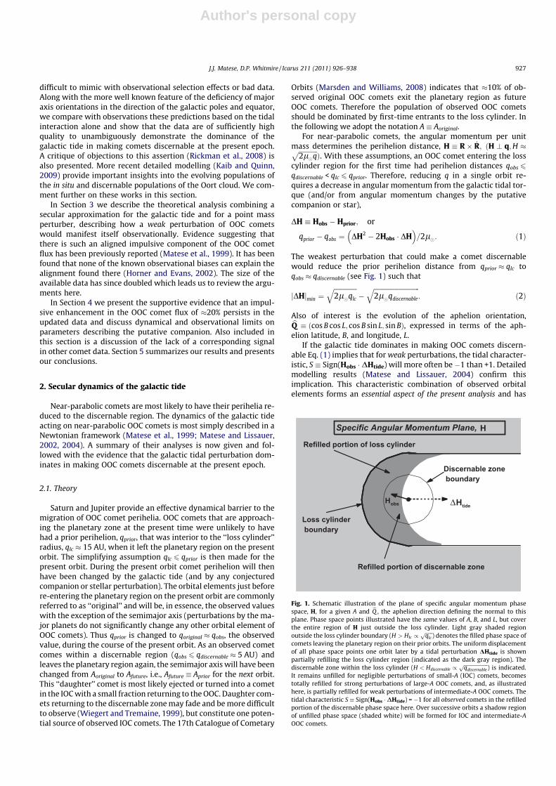
We present updated dynamical and statistical analyses of outer Oort cloud cometary evidence suggestingthat the Sun has a wide-binary jovian mass companion. The results support a conjecture that there existsa companion of mass �1—4 MJupiter orbiting in the innermost region of the outer Oort cloud. Our mostrestrictive prediction is that the orientation angles of the orbit plane in galactic coordinates are centeredon X, the galactic longitude of the ascending node = 319� and i, the galactic inclination = 103� (or theopposite direction) with an uncertainty in the orbit normal direction subtending <2% of the sky. Such acompanion could also have produced the detached Kuiper Belt object Sedna. If the object exists, theabsence of similar evidence in the inner Oort cloud implies that common beliefs about the origin ofobserved inner Oort cloud comets must be reconsidered. Evidence of the putative companion would havebeen recorded by the Wide-field Infrared Survey Explorer (WISE) which has completed its primary mis-sion and is continuing on secondary objectives.

� 2010 Elsevier Inc. All rights reserved.

1. Introduction

Anomalies in the aphelia distribution and orbital elements ofouter Oort cloud (OOC) comets led to the suggestion that �20%of these comets were made discernable due to a weak impulsefrom a bound jovian mass body (Matese et al., 1999). Since thattime the data base of comets has doubled. Further motivation foran updated analysis comes from the Wide-field Infrared SurveyExplorer (WISE; Wright, 2007), which would have easily detectedsuch an object orbiting in the OOC. The conjectured companionwould be incapable of creating comet ‘‘storms’’. To help mitigatepopular confusion with the Nemesis model (Whitmire and Jackson,1984; Davis and Muller, 1984) we use the name recently suggestedby Kirpatrick and Wright (2010), Tyche (the good sister ofNemesis).

In the classical view the Oort cloud (Oort, 1950) is believed tohave been formed as planetesimals were scattered from the solarprotoplanetary disk by the giant planets, ultimately resulting in aflattened inner Oort cloud (IOC) with a more nearly isotropicOOC. A later suggestion was that the Oort cloud instead formedby planetesimal capture from other stars when the Sun was in itsinitial residence in its birth cluster (Zheng et al., 1990), and theconsequences of this option have recently been investigated inmore detail (Levison et al., 2010). The disadvantage of the classicalmodel of Oort cloud formation is that it predicts a scattered disk/Oort cloud population ratio of �0.1, which is roughly a factor of

70 larger than is presently estimated (Levison et al., 2010). Thisproblem is potentially mitigated in the birth cluster model.

The OOC was initially described as the ensemble of comets hav-ing original semimajor axes A P 10,000 AU, but today the bound-ary is taken to be more nearly at 20,000 AU (Kaib and Quinn,2009). It has been shown that the majority of OOC comets thatare made discernable are first-time entrants into the inner plane-tary region (Fernandez, 1981). The dominance of the galactic tidein making OOC comets discernable at the present epoch has beenpredicted on theoretical grounds (Heisler and Tremaine, 1986).Observational evidence of this dominance has been claimed tobe compelling (Delsemme, 1987; Matese and Whitman, 1992;Wiegert and Tremaine, 1999; Matese and Lissauer, 2004).

Matese and Lissauer (2004) adopted an in situ energy distribu-tion similar to the initial distribution of Rickman et al. (2008)and took the remaining phase space external to a ‘‘loss cylinder’’(a dynamical barrier due to Saturn and Jupiter) to be uniformlypopulated at the present epoch. The distribution of cometary orbi-tal elements made discernable from the tide alone was then ob-tained and compared with observations.

Similar modelling (Matese and Lissauer, 2002) had been per-formed including single stellar impulses which mapped the cometflux over a time interval of 5 Myr, in 0.1 Myr intervals. Peak impul-sive enhancements P20% were found to have a half-maximumduration of �2 Myr and occurred with a mean time interval of�15 Myr. Various time-varying distributions of elements werecompared with the modelled tide-alone results and inferencesabout the signatures of a weak stellar impulse were drawn.

In Section 2 we review a discussion (Matese and Lissauer, 2004)of a subtle characteristic of galactic tidal dominance which is

0019-1035/$ - see front matter � 2010 Elsevier Inc. All rights reserved.doi:10.1016/j.icarus.2010.11.009

⇑ Corresponding author. Fax: +1 337 482 6699.E-mail address: matese@louisiana.edu (J.J. Matese).

Icarus 211 (2011) 926–938

Contents lists available at ScienceDirect

Icarus

journal homepage: www.elsevier .com/ locate/ icarus

Author's personal copy

difficult to mimic with observational selection effects or bad data.Along with the more well known feature of the deficiency of majoraxis orientations in the direction of the galactic poles and equator,we compare with observations these predictions based on the tidalinteraction alone and show that the data are of sufficiently highquality to unambiguously demonstrate the dominance of thegalactic tide in making comets discernable at the present epoch.A critique of objections to this assertion (Rickman et al., 2008) isalso presented. More recent detailed modelling (Kaib and Quinn,2009) provide important insights into the evolving populations ofthe in situ and discernable populations of the Oort cloud. We com-ment further on these works in this section.

In Section 3 we describe the theoretical analysis combining asecular approximation for the galactic tide and for a point massperturber, describing how a weak perturbation of OOC cometswould manifest itself observationally. Evidence suggesting thatthere is such an aligned impulsive component of the OOC cometflux has been previously reported (Matese et al., 1999). It has beenfound that none of the known observational biases can explain thealignment found there (Horner and Evans, 2002). The size of theavailable data has since doubled which leads us to review the argu-ments here.

In Section 4 we present the supportive evidence that an impul-sive enhancement in the OOC comet flux of �20% persists in theupdated data and discuss dynamical and observational limits onparameters describing the putative companion. Also included inthis section is a discussion of the lack of a corresponding signalin other comet data. Section 5 summarizes our results and presentsour conclusions.

2. Secular dynamics of the galactic tide

Near-parabolic comets are most likely to have their perihelia re-duced to the discernable region. The dynamics of the galactic tideacting on near-parabolic OOC comets is most simply described in aNewtonian framework (Matese et al., 1999; Matese and Lissauer,2002, 2004). A summary of their analyses is now given and fol-lowed with the evidence that the galactic tidal perturbation dom-inates in making OOC comets discernable at the present epoch.

2.1. Theory

Saturn and Jupiter provide an effective dynamical barrier to themigration of OOC comet perihelia. OOC comets that are approach-ing the planetary zone at the present time were unlikely to havehad a prior perihelion, qprior, that was interior to the ‘‘loss cylinder’’radius, qlc � 15 AU, when it left the planetary region on the presentorbit. The simplifying assumption qlc 6 qprior is then made for thepresent orbit. During the present orbit comet perihelion will thenhave been changed by the galactic tide (and by any conjecturedcompanion or stellar perturbation). The orbital elements just beforere-entering the planetary region on the present orbit are commonlyreferred to as ‘‘original’’ and will be, in essence, the observed valueswith the exception of the semimajor axis (perturbations by the ma-jor planets do not significantly change any other orbital element ofOOC comets). Thus qprior is changed to qoriginal � qobs, the observedvalue, during the course of the present orbit. As an observed cometcomes within a discernable region (qobs 6 qdiscernable � 5 AU) andleaves the planetary region again, the semimajor axis will have beenchanged from Aoriginal to Afuture, i.e., Afuture � Aprior for the next orbit.This ‘‘daughter’’ comet is most likely ejected or turned into a cometin the IOC with a small fraction returning to the OOC. Daughter com-ets returning to the discernable zone may fade and be more difficultto observe (Wiegert and Tremaine, 1999), but constitute one poten-tial source of observed IOC comets. The 17th Catalogue of Cometary

Orbits (Marsden and Williams, 2008) indicates that �10% of ob-served original OOC comets exit the planetary region as futureOOC comets. Therefore the population of observed OOC cometsshould be dominated by first-time entrants to the loss cylinder. Inthe following we adopt the notation A � Aoriginal.

For near-parabolic comets, the angular momentum per unitmass determines the perihelion distance, H � R � _R; ðH ? q;H �ffiffiffiffiffiffiffiffiffiffiffiffi

2l�qp

Þ. With these assumptions, an OOC comet entering the losscylinder region for the first time had perihelion distances qobs 6

qdiscernable < qlc 6 qprior. Therefore, reducing q in a single orbit re-quires a decrease in angular momentum from the galactic tidal tor-que (and/or from angular momentum changes by the putativecompanion or star),

DH � Hobs �Hprior; or

qprior � qobs ¼ DH2 � 2Hobs � DH� �

=2l�: ð1Þ

The weakest perturbation that could make a comet discernablewould reduce the prior perihelion distance from qprior � qlc toqobs � qdiscernable (see Fig. 1) such that

jDHjmin ¼ffiffiffiffiffiffiffiffiffiffiffiffiffiffi2l�qlc

q�

ffiffiffiffiffiffiffiffiffiffiffiffiffiffiffiffiffiffiffiffiffiffiffiffiffiffiffiffi2l�qdiscernable

q: ð2Þ

Also of interest is the evolution of the aphelion orientation,bQ � ðcos B cos L; cos B sin L; sin BÞ, expressed in terms of the aph-elion latitude, B, and longitude, L.

If the galactic tide dominates in making OOC comets discern-able Eq. (1) implies that for weak perturbations, the tidal character-istic, S � Sign(Hobs � DHtide) will more often be �1 than +1. Detailedmodelling results (Matese and Lissauer, 2004) confirm thisimplication. This characteristic combination of observed orbitalelements forms an essential aspect of the present analysis and has

Refilled portion of discernable zone

Hobs

Refilled portion of loss cylinder

ΔHtide

Loss cylinder boundary

Specific Angular Momentum Plane,

Discernable zone boundary

H

Fig. 1. Schematic illustration of the plane of specific angular momentum phasespace, H, for a given A and bQ , the aphelion direction defining the normal to thisplane. Phase space points illustrated have the same values of A, B, and L, but coverthe entire region of H just outside the loss cylinder. Light gray shaded regionoutside the loss cylinder boundary (H > Hlc /

ffiffiffiffiffiffiqlcp

) denotes the filled phase space ofcomets leaving the planetary region on their prior orbits. The uniform displacementof all phase space points one orbit later by a tidal perturbation DHtide is shownpartially refilling the loss cylinder region (indicated as the dark gray region). Thediscernable zone within the loss cylinder (H < Hdiscernable /

ffiffiffiffiffiffiffiffiffiffiffiffiffiffiffiffiffiffiffiqdiscernablep

) is indicated.It remains unfilled for negligible perturbations of small-A (IOC) comets, becomestotally refilled for strong perturbations of large-A OOC comets, and, as illustratedhere, is partially refilled for weak perturbations of intermediate-A OOC comets. Thetidal characteristic S � Sign(Hobs � DHtide) = �1 for all observed comets in the refilledportion of the discernable phase space here. Over successive orbits a shadow regionof unfilled phase space (shaded white) will be formed for IOC and intermediate-AOOC comets.

J.J. Matese, D.P. Whitmire / Icarus 211 (2011) 926–938 927

Author's personal copy

not been included in modelling results presented elsewhere (e.g.,Rickman et al., 2008; Kaib and Quinn, 2009).

A graphical illustration of this theme in Fig. 1 shows the phasespace changes in H for a specific choice of bQ and A over the courseof a single orbit period. As comets recede from the planetary regionon their prior orbits, the interior of the loss cylinder phase spaceregion is essentially emptied of OOC comets by planetary perturba-tions. The adjacent exterior region remains uniformly populated inthis model. To lowest order in q/A, i.e., the near-parabolic phasespace region just outside the loss cylinder boundary, the vector dis-placement in specific angular momentum, DHtide, is independentof the prior value of angular momentum, Hprior, and depends onlyon A and the major axis orientation, bQ , which are taken to be fixedfor the phase space of Fig. 1. In a single orbit all nearby specificangular momentum phase space points, filled and empty, are dis-placed uniformly (Matese and Lissauer, 2004). Fig. 1 illustrates thatin the present modelling, the phrase ‘‘loss cylinder’’ which is usedto describe the Saturn–Jupiter dynamical barrier might be moreappropriately changed to ‘‘loss circle’’.

The magnitude of the single-orbit angular momentum displace-ment is strongly dependent on A, varying as A7/2. Small-A cometsare defined here as IOC comets having galactic perturbations<jDHjmin, unable to repopulate the discernable zone. Large-A OOCcomets are defined here as those having strong tidal perturbationsresulting in large displacements in H that completely refill the dis-cernable zone, making S = 1 equally likely. Intermediate-A OOCcomets are defined here as those that are weakly perturbed bythe tide and only partially refill the discernable zone. Intermedi-ate-A comets preferentially have S = �1, as seen in Fig. 1. In thiscontext intermediate-A OOC comets have the smallest observedvalues of A among OOC comets if the tide dominates in makingcomets discernable. The fuzzy boundaries between small-A, inter-mediate-A and large-A depend weakly on B and L. We choose theboundaries for these intervals based on data discussed in Section 3.

Therefore, independent of stellar influences on the in situ distribu-tion of semimajor axes, if the galactic tidal interaction with the OOCdominates impulsive interactions in producing discernable OOCcomets at the present epoch we should see

a preponderance of OOC comets with S = �1 over those withS = +1, and an association in which S = �1 correlates with the smallest

observed values of A for OOC comets.

Conversely, if perturber impulses dominate in producing OOCcomets at the present epoch, the unique tidal characteristic Sshould be a random variable and should be uncorrelated with A.

2.2. Observational evidence for tidal dominance at the present epoch

Our data are taken from the 17th Catalogue of Cometary Orbitsfrom which we convert the ecliptic Eulerian orbital angles into thegalactic angles B, L and a, the orientation angle of H defined inMatese and Lissauer (2004). The Catalogue lists 102 comets withA > 104 AU (see Appendix B) of the highest quality class, 1A (wecount the split comet C/1996-J1A(B) as a single comet). The qualityclass predominantly distinguishes the accuracy of the originalsemimajor axis determination (Marsden et al., 1978). Since ouranalysis depends sensitively on an accurate determination of A,we restrict our detailed discussions to class 1A comets. In a previ-ous analysis (Matese et al., 1999) the orbital elements of 82 cometsof quality classes 1A + 1B with A > 104 AU given in the 11th Cata-logue were used, 47 of which were class 1A. In the following allreferences to Catalogue data will be to class 1A comets unlessotherwise specified.

The first observational indication that the galactic tide domi-nates involved the distribution in the galactic latitude of aphelion,B (Delsemme, 1987). One finds (Matese et al., 1999) that the dom-inant disk tidal term in the perturbation is /jsinBcosBj (Rickmanet al. (2008) conclude that this perturbation is /jsinBj rather than/jsinBcosBj). B and L are sensibly constant in the course of a singleorbit since Q has significant inertia for near-parabolic orbits. There-fore, if the tide dominates we should expect deficiencies of majoraxis orientations along the galactic poles and the galactic equator,and peaks near B = ±45�. One might argue that observational selec-tion effects can artificially produce an equatorial gap, but polargaps will be more difficult to attribute to an observational selectioneffect.

In Fig. 2 we show the results presented as a distribution injsinBj, which would be uniform for a random distribution. Polarand equatorial gaps are clear, as predicted if the galactic tide dom-inates. A small (but potentially informative) discrepancy is thelocation of the peak. If the tide dominates, our modelling (Mateseand Lissauer, 2004) predicts a peak at jsinBj � 0.7, somewhat largerthan seen in the data. We now look to the tidal characteristic S tofurther emphasize tidal dominance.

The prediction that S = 1 should be equally likely for large-AOOC comets, and that there should be a preponderance of S = �1for intermediate-A OOC comets (see Fig. 1) is now considered. Interms of the original orbital binding energy parameter x � 106 AU/A, class 1A comets have a mean formal error of �5 units, but theuncertainty due to unmodelled outgassing effects is likely to besomewhat larger (Kresák, 1992; Królikowska, 2006). In particularthe fraction of nominally unbound original orbits listed in AppendixB (7 of 102) is likely indicative of the true errors embodied in the tailsof the class 1A OOC comet energy distribution. For comparison, class1B comets nominally have a mean formal error of�12 units but thefraction of unbound original orbits with x < 100 is 13 of 51 suggest-ing that the nominal uncertainty understates the true uncertaintymuch more than for class 1A comets.

In Fig. 3 we show the cumulative binding energy distribution of66 comets with S = �1 and 36 comets with S = +1. The binomialprobability that as many or more would exhibit this imbalance ifin fact S = 1 were equally likely is 2 � 10�3. Further, as predictedby tidal dynamics, this preponderance of S = �1 also correlateswith intermediate-A OOC comets in a statistically significant man-ner. S = 1 is approximately equally likely for comets with x 6 30,suggesting that for this range of semimajor axes the galactic tide isstrong enough to refill the discernable zone almost completely, i.e.,the tidal efficiency is nearly 100% (Matese and Lissauer, 2002). Wetherefore take this as the observationally defined boundary be-tween large-A and intermediate-A OOC comets. In contrast, for30 < x < 100 the evidence is that the tide weakens dramaticallysince 45 comets have S = �1 and only 12 have S = +1. The binomial

0 0.2 0.4 0.6 0.8 1.0sin B

5

10

15

20

25

30

Fig. 2. The distribution in jsinBj for comets listed in Appendix B.

928 J.J. Matese, D.P. Whitmire / Icarus 211 (2011) 926–938

Author's personal copy

probability that as many or more would exhibit this imbalance if infact S = 1 were equally likely for this energy range is 7 � 10�6.This is unambiguous evidence that the class 1A OOC comet dataare of sufficiently high quality and sufficiently free of observationalselection effects to detect this unique imprint of tidal dominance inproducing discernable OOC comets at the present epoch.

Kaib and Quinn (2009) have found that �5% of comets that arediscernable for the first time should have 60 < x, the majority ofwhich have evolved from a primordial location in the IOC. It is un-likely that these comets have had their prior orbit perihelia outsidethe loss cylinder and therefore would not satisfy jDHj > jDHjmin.Taking account of expected errors in the binding energies we adopt30 < x < 60 as the defining interval for intermediate-A OOC cometsand 60 6 x as our working definition for the IOC. Discernable OOCcomets with nominal original energies �1 < x < 60 will be referredto as new comets as they are likely to be first-time entrants into thediscernable zone. Discernable IOC comets with 60 6 x 6 1000 willbe referred to as young comets.

These clear signatures of galactic tidal dominance in makingOOC comets discernable do not mean that we must abandon hopefor detecting any impulsive imprint on the distributions, as we de-scribe in Section 3.

2.3. Comparisons with recent modelling

Kaib and Quinn (2009) have done the most complete modellingof the production of discernable long-period comets (LPC) from theOort cloud in an attempt to infer the Sun’s birth environment. Theyclosely follow whether a new comet was born in the OOC or in theIOC and find that roughly comparable numbers of each primordialpopulation are made discernable after a suitable time lapse. Thebinding energy distribution for the two populations (theirFig. S4) differs in that the distribution for comets born in the IOCpeaks at x � 38 while that for comets born in the OOC peaks atx � 28. They conclude that the IOC pathway provides ‘‘an impor-tant, if not dominant, source of known LPCs’’. The primordial originof discernable comets is not important in our loss-cylindermodelling.

Very few observed comets with 30 < x < 60 are likely to havehad prior perihelia within the loss cylinder. We have used theirFig. S4 as a guide to the energy range most likely to show evidenceof a weak impulsive component of the observed OOC.

Rickman et al. (2008) have also embarked on an ambitiousmodelling program of the long term evolution of the Oort cloudwhich emphasizes a fundamental role for stellar perturbations.They demonstrate that over long timescales stellar impulses areneeded to replenish the phase space of the OOC which is capable

of being made discernable by the galactic tide. Massive star im-pulses serve to efficiently refill this feeding zone for a period ofseveral 100 Myr and therefore provide one aspect of the synergywith the galactic tide that make these comets discernable.

They also assert that ‘‘treating comet injections from the Oortcloud in the contemporary Solar System as a result of the galactictide alone is not a viable idea’’. This statement follows from theirobservations that a tide-alone model evolving over the lifetime ofthe Solar System differs significantly at the present epoch from acombined impulse-tide model.

But their modelling does not shed light on the question of thedominant dynamical mechanism responsible for injecting OOCcomets into the inner planetary region at the present epoch. Theirwork makes detailed predictions using results averaged over170 Myr. Such a large time window inevitably includes many indi-vidual stellar perturbations which contribute directly to the time-averaged flux. Separating out the dominant perturbation makingthese comets discernable at the present epoch would be best ob-tained if they (i) ‘‘turn off’’ both perturbations at the present epoch,(ii) wait for the discerned flux to dissipate, and then (iii) alternatelydetermine subsequent distributions produced by each perturba-tion separately turned on. This analysis was not performed.

Indeed, one can compare our predictions (Matese and Lissauer,2004) for discernable distributions in A and the A-dependent dis-cernable zone refill efficiency with Rickman et al. (2008) (wherethey use the term ‘‘filling factor’’ in the same context as our‘‘efficiency’’). The tide-alone results at the beginning of their simu-lations (see their Fig. 7 and Table III) provide the most appropriatecomparison since their phase space then is most nearly random-ized and comparable to that used in our previous work. One findsthat these two sets of distributions are in good agreement.

Their combined modelling of the latitude distributions doespredict a peak at jsinBj � 0.5, more nearly in agreement withobservations shown in Fig. 2 (however they assert that their pre-dictions do not agree with observations without any discussionof the nature of the discrepancies perceived). If this difference withour tidal model prediction of a peak at jsinBj � 0.7 is supported inthe future it may provide evidence that the in situ phase spacerefilling of the OOC by stellar perturbations is indeed detectablyincomplete at the present epoch, a point emphasized by them. Thiswould not contradict our assertion that the unambiguous evidenceis that the galactic tide dominates in making OOC comets discern-able at the present epoch. It remains for them to demonstratethat the modelling adopted here (Matese and Lissauer, 2002,2004) is no longer viable in describing observations at the presentepoch. We conclude our remarks by noting that neither of theabove analyses have tracked the orbital characteristic S in the pro-duction of new comets, a major measure of galactic dominance inour work.

3. Dynamics of a weak impulsive perturbation

3.1. Theory

The dynamics of a weak perturbation of a near-parabolic cometby a solar companion or field object is now considered. The changein the comet’s specific heliocentric angular momentum induced bya perturber is given by

_Hpert ¼ lpðR � rÞ 1

jR � rj3� 1

r3

!; ð3Þ

where lp = GMp and Mp is the perturber mass located at heliocentricposition r and R is the heliocentric comet position. In terms of the per-turber true anomaly, f, we have r = p/(1 + epcos f), with p = a(1 � ep

2).We then obtain for near-parabolic comets

0 10 20 30 40 50 60 70 80 90 100x

0

10

20

30

40

50

60

70

Nx

Fig. 3. The cumulative binding energy distribution (x � 106 AU/A) for comets listedin Appendix B, separately illustrated for S = 1. Solid line M S = �1, dotted line M

S = +1.

J.J. Matese, D.P. Whitmire / Icarus 211 (2011) 926–938 929

Author's personal copy

dHpert

df¼

ffiffiffiffiffiffiffiffiffil�a

p lp

l�bQ � r

� �Rb

r3

jR � rj3� 1

!; ð4Þ

where b ¼ affiffiffiffiffiffiffiffiffiffiffiffiffiffi1� e2

p

q, the semiminor axis of the perturber. One then

constructs

DHpert ¼ffiffiffiffiffiffiffiffiffil�a

p lp

l�bQ � I; ð5Þ

where the dimensionless integral I is taken around an interval of theperturber true anomaly Df � fo � fi that corresponds to the cometorbital time interval between to � 0, the present epoch, and

ti � �2pffiffiffiffiffiffiffiffiffiffiffiffiffiffiA3=l�

q,

I �Z fo

fi

df rRb

r3

jR � rj3� 1

!: ð6Þ

The first term in I corresponds to the perturber interaction with thecomet, the second with the Sun. For a specified perturber orbital el-lipse, I is determined by the cometary bQ and A as well as the com-panion’s present value of the true anomaly, fo. Eq. (3) is moreconvenient to use in an impulse approximation as has been donein a previous analysis of the combined tide-stellar impulse interac-tion with the OOC (Matese and Lissauer, 2002). Eq. (4) is moreappropriate if one wishes to include the slow ‘‘reflex’’ effects of abound perturber on the Sun.

3.2. Combined tidal and impulsive interaction

The galactic tidal perturbation and any putative point sourceperturbation of the Sun/OOC are, in nature, superposed in thecourse of a cometary orbit. For weak perturbations the two effectscan be superposed in a vector sense, Hobs � Hprior + DHpert + DHti-

de � Hprior + DHnet. The cometary phase space of comets will havethe prior loss cylinder distribution displaced by DHnet. The stan-dard step function for the prior distribution of angular momentumis changed to a uniformly displaced distribution, similar to thatillustrated in Fig. 1, but with DHtide replaced by DHnet,qprior� qobs ¼ ðDH2

net � 2Hobs � DHnetÞ=2l�.

3.3. Weak impulsive effects on the discernable energy and spatialdistributions

Matese and Lissauer (2002) modelled the time-dependentchanges in new comet orbital element distributions that resultedfrom a weak stellar impulse. In particular, the in situ energydistribution was taken to be essentially unchanged, as describedabove. The number of comets in the large-A (x 6 30) interval thatbecame discernable after an impulse was found to be essentiallyunchanged from the case with no impulse, although the specificcomets made discernable were changed. That is, the �100% effi-ciency of refilling the discernable zone remains �100% throughoutthe stellar impulse for large-A comets. This can be visualized inFig. 1 when we consider a large DHtide that completely refills theloss cylinder and the comparative case where the large DHtide ismodified by a weak DHpert. Independent of whether the impulseslightly increased or decreased the perturbation, a large jDHnetjwill still tend to completely refill the loss cylinder, albeit with dif-ferent comets.

For the intermediate-A population the discussion is more sub-tle. Suppose that for a specific bQ a comet population with x � 35will partially fill the discernable zone due to the tide (see Fig. 1).If some of those comets experience an impulse that increasesjDHnetj, the discernable zone will be more completely filled. How-ever other comets will be impulsed such that jDHnetj is decreased.This will in turn decrease the number of discernable comets for

this value of x leaving the efficiency for this x only moderatelyincreased.

Consider now the case for a population with x � 45. The tidalperturbation will be smaller by a factor of �0.4 from the x � 35population, which may be inadequate to make any of these cometsdiscernable in our loss cylinder model. In this case an impulsivetorque preferentially opposed to the tidal torque will have no effecton the number of observed comets for this x since none would havebeen observed in its absence. But for those comets which have aweak impulsive torque preferentially aiding the tide, some willbe made discernable that would not have been in the absence ofan impulse. Therefore the efficiency for this x will increase fromzero, and it will preferentially have S = �1. The net effect for a weakimpulse is to create an enhanced observed OOC comet populationalong the track of the perturber that preferentially has intermedi-ate-A and S = �1. These features have been demonstrated in de-tailed modelling for a weak stellar impulse (Matese and Lissauer,2002). Rickman et al. (2008) also discuss in detail this aspect ofsynergy but do not consider the importance of the characteristic,S, in this discussion.

In reality, the step function distribution of prior orbits for OOCcomets used in the loss cylinder model is a crude first approxima-tion. A small fraction of new comet orbits recede from the plane-tary region as future new comets with perihelia inside the losscylinder. This does not obviate the arguments invoked above.Along with the original energy errors associated with observationaluncertainties and outgassing effects, we can understand why theobserved spread in original OOC energies seen in Fig. 3 is some-what larger than predicted in our loss cylinder model and is consis-tent with more realistic modelling (Kaib and Quinn, 2009).

4. Observational evidence for an impulse

Matese et al. (1999) noted an excess of new comet major axesalong a great circle roughly centered on the galactic longitudinalbins 135� and 315� using 11th Catalogue data of quality classes1A + 1B with x < 100. Further, they found that the excess was pre-dominantly in the intermediate-A OOC population and had a largerproportion of S = �1, consistent with it being impulsively pro-duced. In Fig. 4 we now display the distribution of the aphelia lon-gitudes for comets in Appendix B. We see that the excess remainsin the present data.

4.1. Monte Carlo simulations

There is no obvious a priori reason why a systematic explana-tion of the overpopulation should be associated with a plane pass-ing through the galactic poles. Further, choosing longitude bins forcomparison has an obvious bias in that it preferentially excludes

0 60 120 180 240 300 360L

2

4

6

8

10

12

14

16

18

Fig. 4. The distribution of aphelia longitude, L, for comets listed in Appendix B.

930 J.J. Matese, D.P. Whitmire / Icarus 211 (2011) 926–938

Author's personal copy

solid angles near the poles where the tide is weak. We thereforeconsider great circle fits that count the number of major axes with-in an annular band of width ±9.6�, which has the same solid angle,4p/6, as the two overpopulated aphelia longitude bins in Fig. 4. Thedata that we now analyze includes comets listed in Appendix Bwhich are intermediate-A OOC comets, 30 < x < 60, with S = �1.As described above, this is the subset most likely to exhibit evi-dence of a weak impulsive component. Of these 35 comets, 15were included in the 11th Catalogue considered by Matese et al.(1999). In Fig. 5 we show the aphelia scatter of this data.

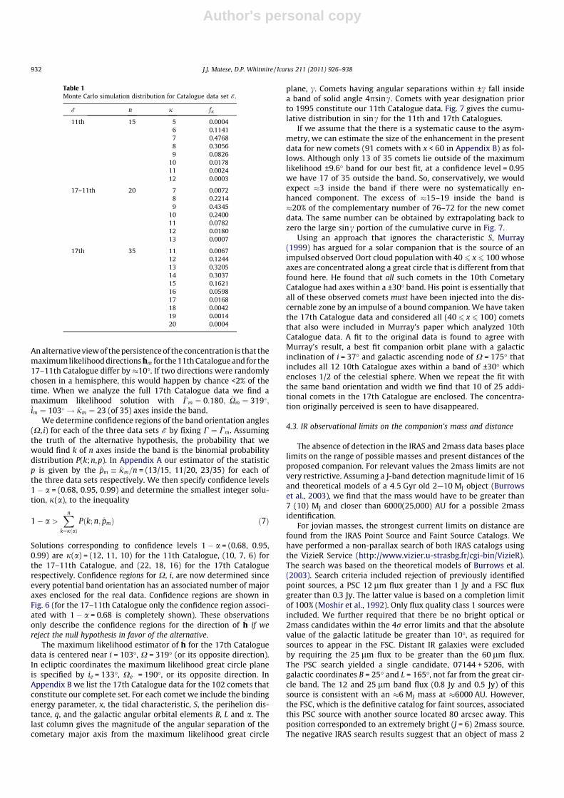
We now consider the null hypothesis, H�, that the dominantgalactic tide can explain the pattern of major axis orientations ofthis data subset and that the observed longitudinal asymmetry isdue to chance alone and not due to a systematic cause. Separatelyinvestigated are the original 11th Catalogue, the present 17th Cat-alogue and the data formed from their difference.

For each of these we perform a variation of the Monte Carlosimulation done elsewhere (Horner and Evans, 2002) which con-sidered the original conjecture. Each comet in the data maintainsits measured value of B, but is randomly assigned a value for L. Thissimulation choice is suited to the null hypothesis that the galactictide acts alone, producing minima in the number of major axes atthe galactic poles and equator and a near-uniform distribution inaphelia longitudes. An analysis is performed for the simulation tofind the orientation of the great circle band orbit normal h of half-width C � sin9.6� = 1/6 which maximizes the number of simulatedmajor axes interior to the band. Counting is done for all possiblegreat circle orientations with normal directions h stepped in a gridcovering solid angles (1�)2. Great circle orientations are denoted bythe galactic longitude of ascending node, X, and the galactic incli-nation, i. The same results are obtained for opposite great circlenormal vectors �h$ ðX� 180�;180� � iÞ.

We then record that maximal number, j. Repeating the process104 times we find the conditional distribution fj (keeping the lati-tudes fixed and assuming the null hypothesis is correct) as esti-mated by the Monte Carlo simulation. The process is repeated forthe 11th Catalogue data which includes n = 15 axes, the complete17th Catalogue data which includes n = 35 axes, as well as forthe 17–11th Catalogue subset. A summary of results is given inTable 1 for each set of evidence E. As an example, for the 11thCatalogue data the Monte Carlo simulations estimate that in only3 of 104 cases would we find as many as 12 major axes in the bandif in fact the null hypothesis was correct. When we repeat the anal-ysis to maximize the number of axes within the band for the realdata, we find that 13 axes are included. The probability of a valuethis large, assuming that H� is true, is apparently very small.

Evidence that the concentration has persisted can be inferredwhen we note that for the 17th Catalogue data the simulationsestimate that in only 4 of 104 cases would we find as many as 20major axes in the band if in fact the null hypothesis was correct.Repeating the analysis to maximize the number of axes withinthe band for the real data we now find that 22 axes are included.

4.2. Inferring the orbit orientation of the concentration

We now discuss the alternative to the null hypothesis, theassumption that there is a systematic cause oriented along a plane.In Appendix A we describe a maximum likelihood analysis to findestimators of the parameters for the orbital angles X, i, and the half-width C of the band under this assumption. For the 11th Cataloguedata we find maximum likelihood estimators Cm ¼ 0:164; Xm ¼318�; im ¼ 95� ! jm ¼ 13 (of 15) axes inside the band. The 17–11th Catalogue maximum likelihood solution gives Xm ¼ 321�;im ¼ 105� ! jm ¼ 11 (of 20) axes inside a band of the same width.

0 90 270 360L

B

Fig. 5. The scatter distribution for aphelia directions of 17th Catalogue new cometshaving a binding energy parameter, x � 106 AU/A, in the interval 30 < x < 60 andtidal characteristic S = �1. Solid curve: ecliptic plane. Dashed curve: maximumlikelihood plane with i = 103�, X = 319�. Black dots: aphelia directions within aband of width ±9.6� covering 1/6 of the celestial sphere and centered on themaximum likelihood great circle path. Gray dots: exterior to the band.

300 310 320 330 34080

90

100

110

120

i

300 310 320 330 34080

90

100

110

120

i

300 310 320 330 34080

90

100

110

120

i

Fig. 6. Confidence regions of orientation angles (X = galactic longitude of ascending node, i = galactic inclination) of great circle bands (black – 68% confidence region, darkgray – 95% confidence region, light gray – 99% confidence region). (left) 11th Catalogue data. (middle) 17–11th Catalogue data. (right) 17th Catalogue data.

0 0.2 0.4 0.6 0.8 1sin

0

5

10

15

20

25

30

35

nsi

n

Fig. 7. The cumulative distribution of the number of major axes of new cometshaving 30 < x < 60 and S = �1 that fall within an annular band of solid angle 4psinccentered on the maximum likelihood great circle i = 103�, X = 319�. Black: 17thCatalogue data. Gray: 11th Catalogue data. Solid lines are for random distributions.Dashed line indicates annular band of maximum likelihood width ±9.6� whichincludes C = 1/6 of the celestial sphere.

J.J. Matese, D.P. Whitmire / Icarus 211 (2011) 926–938 931

Author's personal copy

An alternative view of the persistence of the concentration is that themaximum likelihood directions hm for the 11th Catalogue and for the17–11th Catalogue differ by �10�. If two directions were randomlychosen in a hemisphere, this would happen by chance <2% of thetime. When we analyze the full 17th Catalogue data we find amaximum likelihood solution with Cm ¼ 0:180; Xm ¼ 319�;im ¼ 103� ! jm ¼ 23 (of 35) axes inside the band.

We determine confidence regions of the band orientation angles(X, i) for each of the three data sets E by fixing C ¼ Cm. Assumingthe truth of the alternative hypothesis, the probability that wewould find k of n axes inside the band is the binomial probabilitydistribution P(k;n,p). In Appendix A our estimator of the statisticp is given by the pm � jm=n = (13/15, 11/20, 23/35) for each ofthe three data sets respectively. We then specify confidence levels1 � a = (0.68, 0.95, 0.99) and determine the smallest integer solu-tion, j(a), to the inequality

1� a >Xn

k¼jðaÞPðk; n; pmÞ ð7Þ

Solutions corresponding to confidence levels 1 � a = (0.68, 0.95,0.99) are j(a) = (12, 11, 10) for the 11th Catalogue, (10, 7, 6) forthe 17–11th Catalogue, and (22, 18, 16) for the 17th Cataloguerespectively. Confidence regions for X, i, are now determined sinceevery potential band orientation has an associated number of majoraxes enclosed for the real data. Confidence regions are shown inFig. 6 (for the 17–11th Catalogue only the confidence region associ-ated with 1 � a = 0.68 is completely shown). These observationsonly describe the confidence regions for the direction of h if wereject the null hypothesis in favor of the alternative.

The maximum likelihood estimator of h for the 17th Cataloguedata is centered near i = 103�, X = 319� (or its opposite direction).In ecliptic coordinates the maximum likelihood great circle planeis specified by ie = 133�, Xe = 190�, or its opposite direction. InAppendix B we list the 17th Catalogue data for the 102 comets thatconstitute our complete set. For each comet we include the bindingenergy parameter, x, the tidal characteristic, S, the perihelion dis-tance, q, and the galactic angular orbital elements B, L and a. Thelast column gives the magnitude of the angular separation of thecometary major axis from the maximum likelihood great circle

plane, c. Comets having angular separations within ±c fall insidea band of solid angle 4psinc. Comets with year designation priorto 1995 constitute our 11th Catalogue data. Fig. 7 gives the cumu-lative distribution in sinc for the 11th and 17th Catalogues.

If we assume that the there is a systematic cause to the asym-metry, we can estimate the size of the enhancement in the presentdata for new comets (91 comets with x < 60 in Appendix B) as fol-lows. Although only 13 of 35 comets lie outside of the maximumlikelihood ±9.6� band for our best fit, at a confidence level = 0.95we have 17 of 35 outside the band. So, conservatively, we wouldexpect �3 inside the band if there were no systematically en-hanced component. The excess of �15–19 inside the band is�20% of the complementary number of 76–72 for the new cometdata. The same number can be obtained by extrapolating back tozero the large sinc portion of the cumulative curve in Fig. 7.

Using an approach that ignores the characteristic S, Murray(1999) has argued for a solar companion that is the source of animpulsed observed Oort cloud population with 40 6 x 6 100 whoseaxes are concentrated along a great circle that is different from thatfound here. He found that all such comets in the 10th CometaryCatalogue had axes within a ±30� band. His point is essentially thatall of these observed comets must have been injected into the dis-cernable zone by an impulse of a bound companion. We have takenthe 17th Catalogue data and considered all (40 6 x 6 100) cometsthat also were included in Murray’s paper which analyzed 10thCatalogue data. A fit to the original data is found to agree withMurray’s result, a best fit companion orbit plane with a galacticinclination of i = 37� and galactic ascending node of X = 175� thatincludes all 12 10th Catalogue axes within a band of ±30� whichencloses 1/2 of the celestial sphere. When we repeat the fit withthe same band orientation and width we find that 10 of 25 addi-tional comets in the 17th Catalogue are enclosed. The concentra-tion originally perceived is seen to have disappeared.

4.3. IR observational limits on the companion’s mass and distance

The absence of detection in the IRAS and 2mass data bases placelimits on the range of possible masses and present distances of theproposed companion. For relevant values the 2mass limits are notvery restrictive. Assuming a J-band detection magnitude limit of 16and theoretical models of a 4:5 Gyr old 2—10 MJ object (Burrowset al., 2003), we find that the mass would have to be greater than7 (10) MJ and closer than 6000(25,000) AU for a possible 2massidentification.

For jovian masses, the strongest current limits on distance arefound from the IRAS Point Source and Faint Source Catalogs. Wehave performed a non-parallax search of both IRAS catalogs usingthe VizieR Service (http://www.vizier.u-strasbg.fr/cgi-bin/VizieR).The search was based on the theoretical models of Burrows et al.(2003). Search criteria included rejection of previously identifiedpoint sources, a PSC 12 lm flux greater than 1 Jy and a FSC fluxgreater than 0.3 Jy. The latter value is based on a completion limitof 100% (Moshir et al., 1992). Only flux quality class 1 sources wereincluded. We further required that there be no bright optical or2mass candidates within the 4r error limits and that the absolutevalue of the galactic latitude be greater than 10�, as required forsources to appear in the FSC. Distant IR galaxies were excludedby requiring the 25 lm flux to be greater than the 60 lm flux.The PSC search yielded a single candidate, 07144 + 5206, withgalactic coordinates B = 25� and L = 165�, not far from the great cir-cle band. The 12 and 25 lm band flux (0.8 Jy and 0.5 Jy) of thissource is consistent with an �6 MJ mass at �6000 AU. However,the FSC, which is the definitive catalog for faint sources, associatedthis PSC source with another source located 80 arcsec away. Thisposition corresponded to an extremely bright (J = 6) 2mass source.The negative IRAS search results suggest that an object of mass 2

Table 1Monte Carlo simulation distribution for Catalogue data set E.

E n j fj

11th 15 5 0.00046 0.11417 0.47688 0.30569 0.0826

10 0.017811 0.002412 0.0003

17–11th 20 7 0.00728 0.22149 0.4345

10 0.240011 0.078212 0.018013 0.0007

17th 35 11 0.006712 0.124413 0.320514 0.303715 0.162116 0.059817 0.016818 0.004219 0.001420 0.0004

932 J.J. Matese, D.P. Whitmire / Icarus 211 (2011) 926–938

Author's personal copy

(5) MJ must have a current distance r P 2000(10,000) AU,respectively.

IRAS and 2mass observational constraints prohibit present loca-tions r < 2000:10,000:25,000 AU for Mp = 2:5:10 MJ respectively.Dynamical constraints previously discussed suggest a maximumcompanion mass in the range Mp � 1–4 MJ and semimajor axis inthe range a � 30,000–10,000 AU, respectively. Qualitatively theprobability that there exists a companion with these appropriateparameters is the ratio of the specified companion parameter spacearea (Mp,a) to the complementary, non-IRAS(2mass)-excludedparameter space area. Next we try to roughly estimate this fromthe non-Catalogue evidence.

We assume that there is a certainty that the Sun has an as-yet-to-be-discovered maximum mass companion with mass betweenMPluto $ 20 MJ, the upper limit being fixed by IRAS/2mass observa-tions. What we seek to model is the distribution of the maximumwide-binary companion mass (within these limits) for a collectionof solar-type stars. Zuckerman and Song (2009) give a mass distri-bution for brown dwarfs down to 13 MJ of dN/dM /M�1.2. It mightbe assumed that this power law roughly holds down to the mini-mum Jeans mass limit of 1–4 MJ (Whitworth and Stamatellos,2006) but the mass distribution below 1 MJ is completely un-known. For simplicity we assume that the distribution of maxi-mum masses is dN/dM /M�1 over the entire mass range.

Next we estimate the probability distribution in semimajor axisfor this companion, assumed to be in the interval 102 $ 105 AU,again subject to the IRAS(2mass) limits. We base this estimate onthe known distribution of semimajor axes of wide binary stars.At least 2/3 of solar-type stars in the field reside in binary or multi-ple star systems (Duquennoy and Mayor, 1991). The fraction ofthese systems which have semimajor axes a P 1000 AU (widebinaries) is �15% (Kouwenhoven et al., 2010; Duquennoy andMayor, 1991), and includes periods up to 30 Myr. The origin ofthese wide binaries may be capture during birth cluster dissolution(Kouwenhoven et al., 2010; Levison et al., 2010). For large semima-jor axes the observed distribution is well approximated by (dN/da) / a�1 and we adopt this power law for all maximum massesover the entire interval of a.

The simplifying assumptions we have made are equivalent toassuming a uniform probability distribution over the entireparameter space for the maximum mass companion under consid-eration

d2Nd log Md log a

¼ constant:

Thus the combined probability that the Sun has a companion ofmaximum mass 1–4 MJ with semimajor axis 30,000–10,000 AU issimply the ratio of this parameter area to the entire area after theIRAS constraint has been imposed. This value (�0.015) crudely esti-mates the probability that a jovian mass companion resides in theinferred parameter space. If one believed that the maximum massof an as yet to be discovered object must exceed Neptune’s massthe probability estimate would change to �0.05.

4.4. Dynamical inferences of other perturber properties

Although the orbit normal of the putative companion is tightlyconstrained, other properties are less so. The near-uniform distri-bution of the overpopulation around the great circle suggests thatit has a present orbit that is more nearly circular than parabolic(e2

p < 0:5). The near-circular implication cannot remain true overthe Solar System lifetime since the eccentricity and inclinationosculate significantly due to the tide. Further, the semimajor axiswill be affected by stellar impulses over these timescales.

The implication that e2p < 0:5, is in fact, consistent with the pres-

ent galactic inclination of the perturber inferred here, i � 103�. This

follows from the near-conservation of the z component of galacticangular momentum of objects in the IOC and OOC in the intervalsbetween strong stellar impulses, hz / b cos i / a

ffiffiffiffiffiffiffiffiffiffiffiffiffiffi1� e2

p

qcos i �

constant: Since the present value of jcos103�j � 0.22 is at the lowend of a random distribution, 0 6 jcos ij 6 1, a larger primordial valueof jcos ij implies that the present value of ep is reduced from its pri-mordial value.

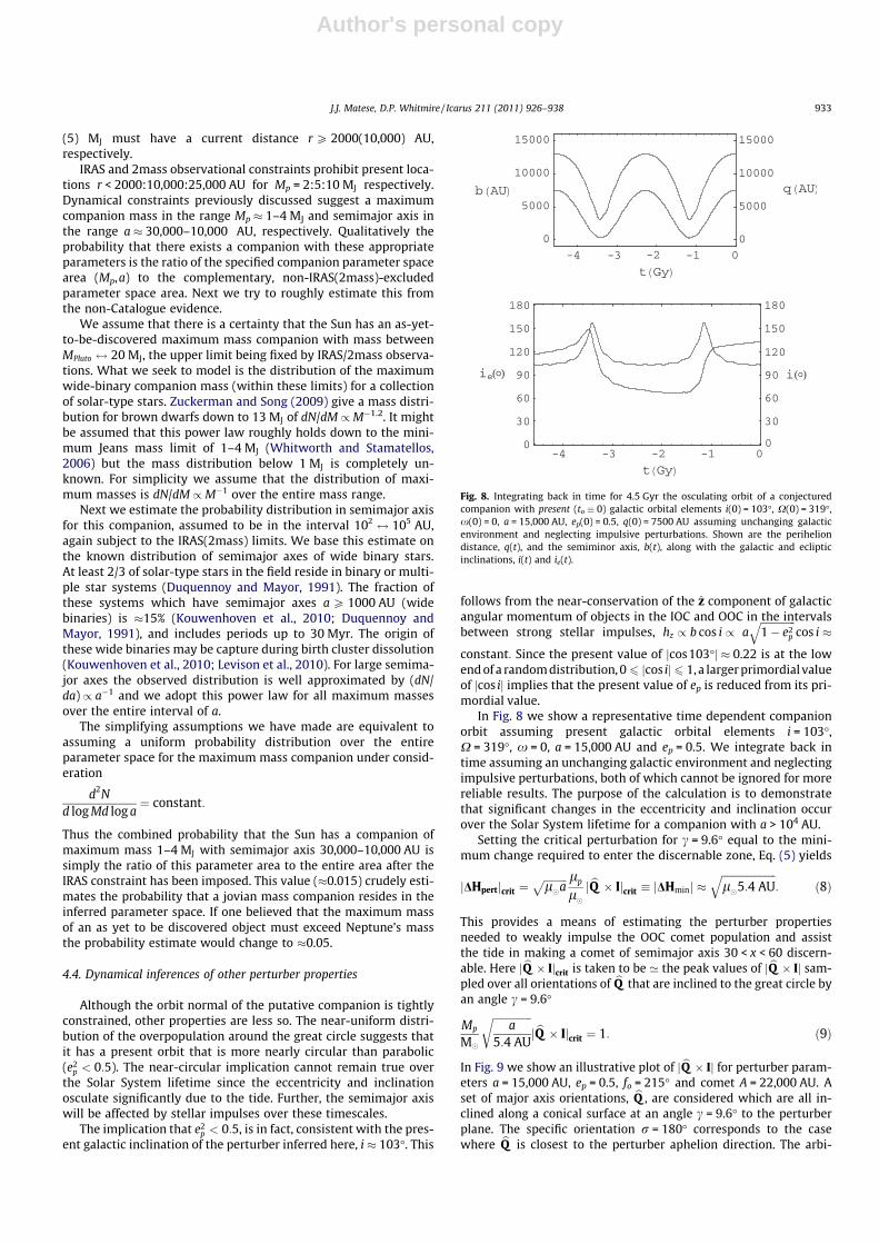
In Fig. 8 we show a representative time dependent companionorbit assuming present galactic orbital elements i = 103�,X = 319�, x = 0, a = 15,000 AU and ep = 0.5. We integrate back intime assuming an unchanging galactic environment and neglectingimpulsive perturbations, both of which cannot be ignored for morereliable results. The purpose of the calculation is to demonstratethat significant changes in the eccentricity and inclination occurover the Solar System lifetime for a companion with a > 104 AU.

Setting the critical perturbation for c = 9.6� equal to the mini-mum change required to enter the discernable zone, Eq. (5) yields

jDHpertjcrit ¼ffiffiffiffiffiffiffiffiffil�a

p lp

l�j bQ � Ijcrit � jDHminj �

ffiffiffiffiffiffiffiffiffiffiffiffiffiffiffiffiffiffiffiffiffil�5:4 AU

q: ð8Þ

This provides a means of estimating the perturber propertiesneeded to weakly impulse the OOC comet population and assistthe tide in making a comet of semimajor axis 30 < x < 60 discern-able. Here j bQ � Ijcrit is taken to be ’ the peak values of j bQ � Ij sam-pled over all orientations of bQ that are inclined to the great circle byan angle c = 9.6�

Mp

M�

ffiffiffiffiffiffiffiffiffiffiffiffiffiffiffia

5:4 AU

rj bQ � Ijcrit ¼ 1: ð9Þ

In Fig. 9 we show an illustrative plot of j bQ � Ij for perturber param-eters a = 15,000 AU, ep = 0.5, fo = 215� and comet A = 22,000 AU. Aset of major axis orientations, bQ , are considered which are all in-clined along a conical surface at an angle c = 9.6� to the perturberplane. The specific orientation r = 180� corresponds to the casewhere bQ is closest to the perturber aphelion direction. The arbi-

-4 -3 -2 -1 0

t Gy

0

30

60

90

120

150

180

ie

0

30

60

90

120

150

180

i

-4 -3 -2 -1 0

t Gy

0

5000

10000

15000

b AU

0

5000

10000

15000

q AU

Fig. 8. Integrating back in time for 4.5 Gyr the osculating orbit of a conjecturedcompanion with present (to � 0) galactic orbital elements i(0) = 103�, X(0) = 319�,x(0) = 0, a = 15,000 AU, ep(0) = 0.5, q(0) = 7500 AU assuming unchanging galacticenvironment and neglecting impulsive perturbations. Shown are the periheliondistance, q(t), and the semiminor axis, b(t), along with the galactic and eclipticinclinations, i(t) and ie(t).

J.J. Matese, D.P. Whitmire / Icarus 211 (2011) 926–938 933

Author's personal copy

trarily chosen present location of the companion is fo = 215� so thatit has recently passed aphelion. Two peaks are shown correspond-ing to the two comet axes bQ that are most strongly impulsed onthe way out and on the way in during the prior cometary orbit.The peak at r = 195� locates the perturber position when cometswere impulsed on their inward leg. The ratio of the comet/perturberperiods is �1.8 in this case and the second peak at r = 35�, corre-sponds to the outward leg when the perturber was on its previousorbit. The importance of the reflex term can be gauged from thebackground contribution. The reflex contribution depends onlymoderately on bQ . In general the peak corresponding to the inwardcomet leg will slightly lag the present perturber position if the per-turber is presently more nearly at aphelion. The second peak corre-sponding to the outward leg will, in general, tend to be randomlypositioned relative to the inward peak if A > a. Each peak containscomet axes bQ that may have had angular momentum impulsesboth aiding the tide and opposing the tide.

The results shown are typical for all ep < 0.5, 90� < fo < 270�when 10,000 AU < a < 30,000 AU. The exceptions include the lesslikely cases when the perturbations on both the outward and in-ward legs of a comet orbit find the perturber at the same generallocation f � r creating a larger net impulse. We shall adopt a typ-ical value of j bQ � Ijcrit � 6—12 for all possible orbit parametersabove. Smaller values in this range typically occur for smaller val-ues of a which have higher relative velocities at orbit crossing. An-other aspect of the variation is that the smaller reflex term can addor subtract from the direct impulse term.

Inserting Mp ¼ 5 MJ into Eq. (9) we obtain a � 6000 AU. Assum-ing e2

p < 0:5, this is marginally inconsistent with IRAS observa-tional limits. Smaller masses should not conflict with IRAS. Thuswe adopt an approximate range of perturber parameters 1 MJ <

Mp < 2 MJ for a � 30,000 AU extending to 2 MJ < Mp < 4 MJ fora � 10,000 AU. This companion mass range is consistent with theminimum Jeans mass (1–7) MJ as variously calculated (Whitworthand Stamatellos, 2006; Low and Lynden-Bell, 1976), although clus-ter capture of ejected planets may be more likely (Kouwenhovenet al., 2010; Levison et al., 2010).

A solar companion remains a viable option (Matese et al., 1999;Horner and Evans, 2002). In addition, we find that an �4 MJ com-panion in an orbit such as that shown in Fig. 8 would be capable ofadiabatically detaching a scattered disk EKBO, producing an objectwith orbital characteristics similar to Sedna (Matese et al., 2006;Gomes et al., 2006). Allowing for the possibility that the perturberwas more tightly bound primordially, smaller masses are thenallowed. It may also be possible to explain the misalignment ofthe invariable plane with the solar spin axis (Gomes et al., 2006)

if the putative companion was more tightly bound primordially.Such a companion would have a temperature of �200 K (Burrowset al., 2003) and its infrared signature would have been recordedby the recently completed Wide-field Infrared Survey Explorer(WISE) mission.

Matese and Lissauer (2002) investigated the frequency of weakstellar showers as well as the patterns of new comet orbital ele-ments. They found that stellar showers that produce a P20% peakenhancement in the background tidal flux occur with a frequencyof approximately once every 15 Myr. The half-maximum durationis�2 Myr. Thus it is only moderately unlikely that we are presentlyin a weak stellar shower of this magnitude. Flux enhancements ofthis magnitude were found to extend over an angular arc �150�and have a full-width half-max of �50�. Weak stellar impulsesnever extend over a larger arc. More simply put, to get the samestellar-induced flux enhancement as inferred from the data here,the enhanced region will have an extent that is �half as long and�twice as wide as that observed. Of course one must considerthe possible alignment of two weaker coincident stellar impulses(or a single weaker statistical anomaly and a coincident singleweaker stellar impulse) that happen to line up on opposite hemi-spheres. These will be improbable. For example, suppose we as-sume that there will always be two weak stellar impulsesenhancing the observed background tidal flux, each with half theobserved enhancement. The probability that both stellar orbitplanes will be aligned to within ±9.6� is 0.014.

4.5. The absence of an impulsive component in other data

Young comets have been defined here as observed IOC cometswith 60 6 x 6 1000. The 17th Catalogue lists 64 young comets, 49of which have S = �1, 15 of which have S = +1, a ratio that exceedsthat of new comets (56 for S = �1, 35 for S = +1). Further, 13 youngcomets have future orbits that are unbound, 4 become bound newcomets, 38 return to the young population and 9 become moretightly bound. Of the 91 observed new comets 50 have future orbitsthat are unbound, 8 return to the bound new population and 33 be-come young comets. None become more tightly bound than youngcomets. To complete the overview, the median perihelion distancefor S = �1 young comets is �2.8 AU, while that for the S = +1 youngcomets is �2.7 AU. The corresponding results are �3.8 AU for the56 S = �1 new comets and �2.5 AU for the 35 S = +1 new comets.There is no evidence of an overpopulation of S = �1 young comets(or of lower quality classes of new comets) within the perceivedband. These observations require further discussion.

4.5.1. Young cometsOnly 7 of 49 young comets with S = �1 are in the band – the

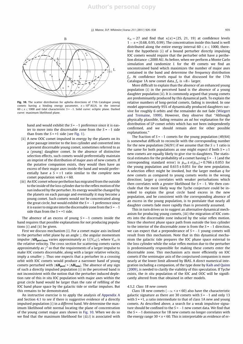
band is underpopulated with young comets. The scatter in aph-elion directions of these young comets is shown in Fig. 10. One ob-serves a modest selection effect in which young comet aphelia aredeficient in the equatorial north hemisphere, with polar directionlocated at galactic coordinates L = 123�, B = 27�. Young cometsare less likely to be discovered if their perihelia are in the equato-rial south hemisphere.

Any mechanism which is invoked for producing young cometsshould be able to explain the data which indicates that young com-ets preferentially have S = �1 to a degree that may exceed that ofnew comets. Three possible dynamical mechanisms for producingyoung comets include.

(i) An IOC comet with perihelion outside the loss cylinderweakly impulsed on its present orbit by a bound perturbersuch that it became a discernable young comet. These com-ets would preferentially have their major axes inside the

0 50 100 150 200 250 300 3500

2

4

6

8

10

12

14

Q Ι

Fig. 9. An example case showing the single-orbit impulse strength j bQ � Ij forcomets with A = 22,000 AU and bQ inclined to the perturber plane by c = 9.6�. Thepositions r = 0(180�) correspond to comet major axis orientations closest to theperturber perihelion (aphelion). Perturber parameters are a = 15,000 AU, ep = 0.5,and fo = 215�, the present true anomaly of the perturber.

934 J.J. Matese, D.P. Whitmire / Icarus 211 (2011) 926–938

Author's personal copy

band and would exhibit the S = �1 preference since it is eas-ier to move into the discernable zone from the S = �1 sidethan from the S = +1 side (see Fig. 1).

(ii) A new OOC comet impulsed in energy by the planets on itsprior passage interior to the loss cylinder and converted intoa present discernable young comet, sometimes referred to asa (young) daughter comet. In the absence of distinctiveselection effects, such comets would preferentially maintainan imprint of the distribution of major axes of new comets. Ifthe putative companion exists, they would then have anexcess of their major axes inside the band and would prefer-entially have a S = 1 ratio similar to the complete newcomet population with x < 60.

(iii) An IOC comet whose perihelion has migrated from the outsideto the inside of the loss cylinder due to the reflex motion of thesun induced by the perturber. Its energy would be changed bythe planets on each passage and eventually it may become ayoung comet. Such comets would not be concentrated alongthe great circle, but would exhibit the S = �1 preference sinceit is easier to migrate into the discernable zone from the S = �1side than from the S = +1 side.

The absence of an excess of young S = �1 comets inside theband requires that possible explanations for not producing popula-tions (i) and (ii) be given.

First we discuss mechanism (i). For a comet major axis inclinedto the perturber orbit plane by an angle c, the angular momentumimpulse jDHpertjmax varies approximately as 1/(Vrelc), where Vrel isthe relative velocity. The cross section for scattering comets variesapproximately as c2 so that the requirements of a larger impulse tomake IOC comets discernable, along with a larger relative velocity,imply a smaller c. Thus one expects that a perturber in a crossingorbit with IOC comets would produce a narrower band of youngcomets perturbed with jDHpertj > jDHminj. The absence of any signof such a directly impulsed population (i) in the perceived band isnot inconsistent with the notion that the perturber induced deple-tion rate of this in situ IOC population with major axes within thegreat circle band would be larger than the rate of refilling of theIOC band phase space by the galactic tide or stellar impulses. Butthis remains to be demonstrated.

An instructive exercise is to apply the analysis of Appendix Aand Section 4.1 to see if there is suggestive evidence of a directlyimpulsed population (i) in a different band. We determine the max-imum likelihood orbit normal locating the plane of concentrationof the young comet major axes shown in Fig. 10. When we do sowe find that the maximum likelihood for (X, i) is associated with

jm ¼ 27 and find that j(a) = (25, 21, 19) at confidence levels1 � a = (0.68, 0.95, 0.99). The concentration inside this band is welldistributed along the entire energy interval 60 6 x 6 1000, there-fore the hypothesis (i) of a bound perturber directly impulsingIOC comets would require that the perturber orbit have a perihe-lion distance62000 AU. As before, when we perform a Monte Carlosimulation and randomize L for the 49 comets we find anunconstrained band which maximizes the number of major axescontained in the band and determine the frequency distributionfj. At confidence levels equal to that discussed for the 17thCatalogue 1A new comet data, fj is �8� larger.

More difficult to explain than the absence of an enhanced youngpopulation (i) in the perceived band is the absence of a youngdaughter population (ii). It is commonly argued that young cometsare predominantly produced by this dynamical path. To explain therelative numbers of long-period comets, fading is invoked. In onemodel approximately 95% of dynamically produced daughters sur-vive for roughly 6 orbits and the remainder do not fade (Wiegertand Tremaine, 1999). However, they observe that ‘‘Althoughphysically plausible, fading remains an ad hoc explanation for thedistribution of LP comet orbits which has not been independentlyconfirmed, and we should remain alert for other possibleexplanations.’’

The fraction of S = �1 comets for the young population (49/64)is somewhat difficult to reconcile with the corresponding numberfor the new population (56/91) if we assume that the S 1 ratio isthe same for both populations as one might expect if both S = 1new comets are equally likely to give rise to daughters. The statis-tical estimates for the probability of a comet having S = �1 (and thecorresponding standard error) is pest ± r(pest) = 0.766 ± 0.053 forthe young population and 0.615 ± 0.051 for the new population.A selection effect might be invoked, but the larger median q fornew comets as compared to young comets works in the wrongdirection; larger q correlates with weaker perturbations whichthen correlates with a greater likelihood for S = �1. We then con-clude that the most likely way the Tyche conjecture could be in-voked to explain the great circle band excess in the newpopulation, and be consistent with the corresponding absence ofan excess in the young population, is to postulate that nearly alldaughter comets fade more rapidly than is presently assumed.

This in turn drives us to suggest an alternative dynamical mech-anism for producing young comets, (iii) the migration of IOC com-ets into the discernable zone induced by the solar reflex motion.Since the shortest phase space path from outside the loss cylinderto the interior of the discernable zone is from the S = �1 direction,we can expect that a preponderance of S = �1 young comets willresult from this mechanism. Note that in this dynamical mecha-nism the galactic tide prepares the IOC phase space external tothe loss cylinder while the solar reflex motion due to the perturberis predominantly responsible for making these comets enter thediscernable zone. This mechanism acts more efficiently on IOCcomets if the semimajor axis of the conjectured companion is morenearly at the lower limit allowed by IRAS. A direct numerical inte-gration including a companion, of the type done by Kaib and Quinn(2009), is needed to clarify the viability of this speculation. If Tycheexists, the in situ population of the IOC and OOC will be signifi-cantly altered from that obtained in other models.

4.5.2. Class 1B new cometsClass 1B new comets (�1 < x < 60) also have the characteristic

galactic signature as there are 30 comets with S = �1 and only 13with S = +1, a ratio intermediate to that of class 1A new and youngcomets. As described above, a search for a weak impulsive signa-ture should be confined to the S = �1 new comet data. We find thatthe S = �1 dominance for 1B new comets no longer correlates withthe energy range 30 < x < 60. This is interpretable as evidence of er-

0 90 270 360L

B

Fig. 10. The scatter distribution for aphelia directions of 17th Catalogue youngcomets having a binding energy parameter, x � 106 AU/A, in the interval60 6 x 6 1000 and tidal characteristic S = �1. Solid curve: ecliptic plane. Dashedcurve: maximum likelihood plane.

J.J. Matese, D.P. Whitmire / Icarus 211 (2011) 926–938 935

Author's personal copy

rors in the determination of x for this quality class, as previouslydiscussed. A clearer picture of the true uncertainty, includingunmodelled outgassing effects, is suggested by the observationsthat only 2 of the 56 S = �1 class 1A new comets are nominally un-bound, while 11 of the 30 S = �1 class 1B new comets are nomi-nally unbound. Further evidence that outgassing is moreimportant for class 1B new comets is the fact that the median peri-helion distance of the S = �1 class 1B new comets is 1.5 AU, whilethat of the S = �1 class 1A new comets is 3.8 AU. These observa-tions suggest that the 1B new comet population may be muchmore contaminated by truly young comets because of outgassingenergy errors than is the class 1A new comet population.

When we do a maximum likelihood search for the orbit normalh using the same procedure described in Appendix A with the evi-dence being the 30 S = �1 class 1B new comet major axes, the max-imum likelihood orientation has jm ¼ 14 axes falling within theband, but again the band orientation is well removed from thatfound for class 1A new comets. A confidence level of 0.99 is asso-ciated with j(a) = 8, extends over a large solid angle, and has aninsignificant P-value. The maximum likelihood band orientationobtained for the 30 < x < 60 class 1A evidence does include 8 ofthese 30 axes.

A selection effect that partially explains the different levels ofenhancement in the class 1A and 1B evidence is as follows: Class1A new comets have less outgassing M larger perihelion distances.But larger perihelion distances correlate with weak perturbations,those that are most likely to exhibit the effect of a bound perturber.Therefore class 1A evidence preferentially selects weak perturba-tions.

5. Summary and conclusions

We have described how the dynamics of a dominant galactic ti-dal interaction, weakly aided by an impulsive perturbation, pre-dicts specific properties for distributions of galactic orbitalelements of observed outer Oort cloud comets. These subtle pre-dictions have been found to be manifest in high-quality observa-tional data, suggesting that the observed OOC comet populationcontains an anomalous excess of �20% oriented along a well-de-fined arc. The extent of the enhanced arc is inconsistent with aweak stellar impulse, but is consistent with a jovian mass solarcompanion orbiting in the Oort cloud. A putative companion withthese properties may also be capable of producing detached KuiperBelt objects such as Sedna and has been given the name Tyche.Tyche would have depleted the inner Oort cloud over the Solar Sys-tem lifetime requiring a corresponding increase in the inferred pri-mordial Oort cloud population. A substantive difficulty with theTyche conjecture is the absence of a corresponding impulsivelyproduced excess in the observed IOC comet population.

Acknowledgments

The authors thank Jack J. Lissauer for his continuing interest andfor his contributions to this research. Additionally, useful refereecomments were provided by Julio Fernandez. We also acknowl-edge the guidance in statistical matters that has been providedby Charles L. Anderson.

Appendix A. Maximum likelihood analysis for the orbit planeorientation.

The relevant parameters of the putative companion are ep, Mp, a,X, i. In Sections 4.3 and 4.4 we discuss the rationale for estimatingthe allowed ranges of values for ep, Mp, a and these can loosely betaken as the 1r confidence intervals. Here we discuss the more

restrictive limits on orbital parameters, those inferred from a likeli-hood analysis involving the orbit plane orientation angles X, i asso-ciated with the orbit plane normal h. The evidence underconsideration is composed of the set of major axis orientations,E ¼ Q j; ðj ¼ 1;nÞ. Let zj �j Q j � h j� sin cj, a measure of the misalign-ment of the jth comet major axis with the assumed plane. Note that zj

implicitly depends on the unknown orbital parameters X, i. Our goalis to determine a maximal measure of the degree of concentration ofthese axes along the unknown plane. In Fig. 7 we show the cumula-tive number distribution of major axes for a specific choice ofh;nð6 sin c; hÞ.

The probability density function describing the likelihood ofmeasuring zj given p, X, i, C is defined as1

f ðEjp;X; i;CÞ �pC C P zj P 0;1�p1�C 1 P zj > C;

(

where 0 < p < 1, X, i, C are free parameters whose values are to bedetermined by maximizing the likelihood function

Lðp;X; i;CjEÞ �Yn

j¼1

f ðEjp;X; i;CÞ ¼ pC

� �j 1� p1� C

� �n�j

:

Here j � nð6 C; hÞ 6 n is the number of axes inside the band ofhalfwidth C having orientation angles X, i.

The maximum likelihood estimator of the parameter p (for arbi-trary X, i, C) is then j/n such that

Lðp! j=n;X; i;CjEÞ ¼ j=nC

� �j 1� j=n1� C

� �n�j

:

A maximum in the likelihood function is expected to occur in thevicinity of the parameter estimators Cm � 1=6; Xm � 315�;im � 90� based on Fig. 4 and prior work (Matese et al., 1999). To findthe maximum likelihood for E ¼ 11th we scan this vicinity andmaximize the likelihood when the parameters take on the valuesCm ¼ 0:164; Xm ¼ 318�; im ¼ 95� ! jm ¼ 13; pm ¼ 13=15.

Table 2Appendix B: Orbital elements of all 17th Catalogue class 1A comets with x < 100. Allangles are in degrees.

Comet name x S q (AU) B L a c

C/1996 J1-A(J1-B)

�510 (�1) �1 1.2978 15.9 202.6 55.0 51.13

C/1996 E1 �42 1 1.3590 �22.6 304.3 319.2 18.39C/1942 C2 �34 1 4.1134 �24.5 18.8 335.2 42.27C/1946 C1 �13 1 1.7241 �60.3 313.1 276.7 14.17C/2005 B1 �13 1 3.2049 �17.6 282.6 12.7 38.28C/1946 U1 �1 1 2.4077 49.0 347.2 255.0 28.13C/1997 BA6 0 �1 3.4364 27.7 123.0 52.9 20.05C/1993 Q1 3 1 0.9673 41.2 112.7 174.6 28.22C/2005 K1 7 1 3.6929 �17.3 227.4 312.1 85.45C/2003 T3 10 1 1.4811 25.5 293.6 148.9 16.25C/2006 L2 10 �1 1.9939 �50.0 225.1 98.2 52.89C/1974 V1 11 �1 6.0189 28.0 308.9 63.1 2.61C/1988 B1 13 �1 5.0308 �47.6 316.3 122.1 11.37C/2006 K1 13 1 4.4255 66.1 56.2 247.3 36.69C/2004 X3 14 1 4.4023 �36.8 80.9 24.1 31.90C/2005 E2 14 1 1.5196 42.0 312.6 134.6 3.99C/2006 OF2 15 1 2.4314 10.5 322.5 133.0 5.75C/1991 F2 16 �1 1.5177 29.7 90.0 345.1 48.65C/2005 G1 16 �1 4.9607 �55.3 297.9 100.6 22.60C/1916 G1 17 �1 1.6864 17.9 225.9 30.1 58.95C/1956 F1-A 17 1 4.4473 �25.4 180.0 62.1 42.33C/1944 K2 18 �1 2.2259 �31.8 124.3 159.3 5.25C/2007 O1 18 �1 2.8767 2.1 197.3 7.6 55.06C/1935 Q1 19 1 4.0434 11.8 248.0 115.3 58.81C/1999 J2 19 �1 7.1098 �49.9 234.4 259.3 52.80

936 J.J. Matese, D.P. Whitmire / Icarus 211 (2011) 926–938

Author's personal copy

Now we repeat the above analysis for E = 17th. In a preliminarycalculation, we fix C = 1/6, and find that the likelihood is maxi-mized when X = 319�, i = 103� ? j = 22. This is the great circle fitshown in Fig. 5. A slightly larger maximum likelihood is foundwhen we increase the halfwidth to Cm ¼ 0:180! jm ¼ 23;pm ¼ 23=35 for the same direction of h. A separate question nowis the maximum likelihood direction of the more recent evidence,E = 17–11th. Again we fix C = 1/6 and maximize the likelihood tofind Xm ¼ 321�; im ¼ 105� ! jm ¼ 11; pm ¼ 11=20.

Concluding, we note that this analysis only yields maximumlikelihood estimators for C, X, i, p under the assumption that thedata requires a systematic cause oriented along a plane, the alter-native to the null hypothesis discussed in Section 4.1.

Appendix B

See Table 2.

References

Burrows, A., Sudarsky, D., Lunine, J.J., 2003. Beyond the T dwarfs: Theoreticalspectra, colors and detectability of the coolest brown dwarfs. Astrophys. J. 596,587–596. <http://zenith.as.arizona.edu/�burrows/evolution3.html>.

Davis, P.Hut, Muller, R., 1984. Extinction of species by periodic comet showers.Nature 308, 715–717.

Delsemme, A.H., 1987. Galactic tides affect the Oort cloud: An observationalconfirmation. Astron. Astrophys. 187, 913–918.

Duquennoy, A., Mayor, M., 1991. Multiplicity among solar-type stars in the solarneighborhood: II. Distribution of the orbital elements in an unbiased sample.Astron. Astrophys. 248, 485–524.

Fernandez, J., 1981. New and evolved comets in the Solar System. Astron. Astrophys.96, 26–35.

Gomes, R.S., Matese, J.J., Lissauer, J.J., 2006. A distant planetary-mass solarcompanion may have produced distant detached objects. Icarus 184, 589–601.

Heisler, J., Tremaine, S., 1986. Influence of the galactic tidal field on the Oort cloud.Icarus 65, 13–26.

Horner, J., Evans, N.W., 2002. Biases in cometary Catalogues and Planet X. Mon. Not.R. Astron. Soc. 335, 641–654.

Kaib, N.A., Quinn, T., 2009. Reassessing the source of long-period comets. Science325, 1234–1236.

Kirpatrick, D., Wright, N., 2010. (Quoted in) Sun’s Nemesis pelted Earth withcomets, study suggests. <Space.com/scienceastronomy/nemesis-comets-earth-am-100311.html>.

Kouwenhoven, M.B.N., Goodwin, S.P., Parker, R.J., Davies, M.B., Malmberg, D.,Kroupa P., 2010. The formation of very wide binaries during the star clusterdissolution phase. arXiv:1001.3969V1[astro-ph.GA]

Kresák, L., 1992. Are there any comets coming from interstellar space? Astron.Astrophys. 259, 682–691.

Królikowska, M., 2006. Non-gravitational effects in long-period comets and the sizeof the Oort cloud. Acta Astron. 56, 385–412.

Levison, H.F., Duncan, M.J., Brasser, R., Kaufman, D.E., 2010. Capture of the Sun’sOort cloud from stars in its birth cluster. Science 329, 187–190.

Low, C., Lynden-Bell, D., 1976. The minimum Jeans mass when fragmentation muststop. Mon. Not. R. Astron. Soc. 176, 367–390.

Marsden, B.G., Williams, G.V., 2008. Catalogue of Cometary Orbits, 17th ed.Smithsonian Astrophysical Observatory, Cambridge, MA.

Marsden, B.G., Sekanina, Z., Everhart, E., 1978. New osculating orbits for 110 cometsand analysis of original orbits for 200 comets. Astron. J. 83, 64–71.

Matese, J.J., Lissauer, J.J., 2002. Characteristics and frequency of weak stellarimpulses of the Oort cloud. Icarus 157, 228–240.

Matese, J.J., Lissauer, J.J., 2004. Perihelion evolution of observed new comets impliesthe dominance of the galactic tide in making Oort cloud comets observable.Icarus 170, 508–513.

Matese, J.J., Whitman, P.G., 1992. A model of the galactic tidal interaction with theOort comet cloud. Celest. Mech. Dynam. Astron. 54, 13–36.

Matese, J.J., Whitman, P.G., Whitmire, D.P., 1999. Cometary evidence of a massivebody in the outer Oort cloud. Icarus 141, 354–366.

Matese, J.J., Whitmire, D.P., Lissauer, J.J., 2006. A wide binary solar companion as apossible origin of Sedna-like objects. Earth Moon Planets 97, 459–470.

Moshir, M. et al., 1992. Explanatory Supplement to the IRAS Faint Source Surveyversion 2. JPL D-10015 8/92 (Pasadena:JPL), Figure III.C.1.

Murray, J.B., 1999. Arguments for the presence of a distant large undiscovered SolarSystem planet. Mon. Not. R. Astron. Soc. 309, 31–34.

Oort, J.H., 1950. The structure of the cloud of comets surrounding the Solar System,and a hypothesis concerning its structure. Bull. Astron. Inst. Neth. 11, 91–110.

Rickman, H.M., Fouchard, M., Froeschlé, C., Valsecchi, G.B., 2008. Injection of Oortcloud comets: The fundamental role of stellar perturbations. Celest. Mech.Dynam. Astron. 102, 111–132.

Whitmire, D., Jackson, A., 1984. Are periodic mass extinctions driven by a distantsolar companion? Nature 308, 713–715.

Table 2 (continued)

Comet name x S q (AU) B L a c

C/1973 E1 20 �1 0.1424 17.0 207.3 46.3 53.15C/1984 W2 20 1 4.0002 33.1 79.5 101.0 55.69C/2001 C1 20 1 5.1046 �8.3 135.0 344.1 2.02C/2004 P1 20 �1 6.0141 20.2 208.7 63.7 51.26C/1922 U1 21 �1 2.2588 16.3 270.6 52.4 39.46C/1997 A1 21 1 3.1572 �19.9 352.3 306.7 25.22C/2003 K4 23 1 1.0236 �46.8 104.3 307.2 12.49C/2005 Q1 23 �1 6.4084 �8.8 321.7 258.1 0.65C/1947 S1 24 1 0.7481 10.9 185.4 170.2 40.61C/1978 H1 24 1 1.1365 �20.7 124.4 30.2 8.65C/1999 K5 24 �1 3.2554 34.1 129.8 271.8 14.81C/2001 G1 24 �1 8.2356 �46.8 113.6 118.9 7.02C/2006 HW51 25 1 2.2656 �35.4 162.3 83.4 26.39C/1914 M1 27 �1 3.7468 �1.4 200.9 100.9 59.81C/1980 E1 27 1 3.3639 �18.2 177.0 29.9 39.78C/2004 YJ35 27 �1 1.7812 �38.2 346.3 122.2 12.23C/1992 J1 28 1 3.0070 �43.8 316.9 0.3 10.47C/1913 Y1 29 �1 1.1045 �52.4 283.0 237.4 31.83C/1987 W3 29 �1 3.3328 64.7 333.5 62.5 17.92C/2001 K5 29 1 5.1843 �30.3 223.1 78.8 71.80C/1989 X1 32 �1 0.3498 �41.0 325.6 218.0 3.57C/1978 A1 33 �1 5.6064 �31.4 142.3 167.8 9.48C/1993 K1 33 �1 4.8493 2.3 130.9 347.4 8.38C/1948 E1 34 1 2.1071 �38.6 250.2 83.2 58.25C/1948 T1 34 �1 3.2611 17.9 324.0 306.9 8.63C/2006 Q1 34 �1 2.7636 �45.5 112.2 134.0 8.48C/1925 F1 35 1 4.1808 �40.9 65.6 327.8 33.96C/2002 J4 35 �1 3.6338 32.4 162.6 342.6 12.07C/1974 F1 36 �1 3.0115 21.7 140.3 10.7 3.59C/2003 S3 36 �1 8.1294 11.6 345.3 351.9 27.95C/2004 B1 36 1 1.6019 27.7 167.1 138.4 17.55C/1950 K1 37 �1 2.5723 �43.8 137.7 269.9 8.02C/1999 U4 37 �1 4.9153 �30.2 322.6 183.8 3.42C/2006 E1 37 �1 6.0406 31.4 140.5 290.6 21.24C/2006 P1 37 1 0.1707 �5.0 342.2 72.9 5.47C/1999 F1 38 �1 5.7869 15.2 99.7 341.0 68.86C/1999 U1 38 �1 4.1376 25.1 67.4 291.1 40.91C/2000 CT54 38 �1 3.1561 36.7 145.1 8.0 2.96C/2002 L9 38 �1 7.0330 51.6 147.6 292.5 4.93C/1954 Y1 39 �1 4.0769 �23.5 314.1 232.3 9.55C/1925 G1 40 1 1.1095 10.5 238.3 151.2 64.77C/1997 J2 40 1 3.0511 �0.5 261.1 332.6 55.83C/1954 O2 42 1 3.8699 �18.4 336.4 53.3 11.82C/1979 M3 42 1 4.6869 14.1 207.0 126.6 55.24C/2000 K1 42 �1 6.2761 �21.6 190.7 144.5 52.50C/2006 S3 42 �1 5.1309 �15.3 188.0 219.4 50.21C/1946 P1 44 �1 1.1361 �20.0 126.6 108.7 6.85C/1999 Y1 44 �1 3.0912 62.7 289.2 326.2 1.31C/2000 A1 44 �1 9.7431 �33.0 19.7 171.9 36.22C/2005 EL173 44 �1 3.8863 23.3 50.4 350.5 79.60C/1932 M2 45 �1 2.3136 �14.6 146.5 172.1 10.33C/1987 H1 46 �1 5.4575 �17.6 190.9 161.4 53.02C/1888 R1 48 �1 1.8149 59.5 313.7 289.0 8.54C/1983 O1 48 �1 3.3179 55.2 324.4 355.4 13.71C/1973 A1 49 �1 2.5111 �50.7 106.2 220.9 9.24C/1989 Y1 49 1 1.5692 �6.1 328.9 96.2 8.22C/2007 D1 50 �1 8.7936 �41.3 64.4 157.8 33.83C/2003 WT42 51 �1 5.1909 �56.8 353.7 171.0 6.59C/2000 O1 52 �1 5.9217 23.5 313.8 286.2 25.23C/2000 SV74 52 �1 3.5417 �21.5 296.7 193.5 0.53C/1999 F2 54 �1 4.7188 �46.0 135.3 112.9 6.83C/1999 S2 56 �1 6.4662 22.2 153.2 322.9 7.83C/2006 K3 56 1 2.5015 46.6 22.7 261.9 49.79C/1976 D2 59 1 6.8807 �44.5 120.9 315.8 3.36C/1987 F1 59 �1 3.6246 �26.5 129.8 186.4 2.20C/1993 F1 59 �1 5.9005 �45.0 330.2 213.7 1.44C/2002 J5 60 �1 5.7268 �33.0 240.2 157.1 67.57C/2005 L3 60 �1 5.5933 �30.3 203.9 169.6 61.07C/2000 Y1 61 �1 7.9748 28.0 350.3 8.5 33.52C/1999 H3 65 �1 3.5009 �50.1 250.1 167.3 49.12C/1898 L1 68 �1 1.7016 28.3 143.8 315.4 2.01C/1999 N4 68 �1 5.5047 �23.3 200.6 204.1 61.14C/1972 L1 69 1 4.2757 �40.3 235.4 66.6 62.09C/2007 JA21 69 �1 5.3682 �31.4 272.5 247.5 46.07C/1958 R1 76 �1 1.6282 �18.4 307.6 133.4 14.74C/1955 G1 82 �1 4.4957 �29.8 233.2 168.5 72.73C/2005 A1-A 94 �1 0.9069 29.4 113.9 12.6 28.06

J.J. Matese, D.P. Whitmire / Icarus 211 (2011) 926–938 937

Author's personal copy

Whitworth, A.P., Stamatellos, D., 2006. The minimum mass for star formation, andthe origin of binary brown dwarfs. Astron. Astrophys. 458, 817–829.

Wiegert, P., Tremaine, S., 1999. The evolution of long-period comets. Icarus 137, 84–122.

Wright, E.L., 2007. Wide-field Infrared Survey Explorer. <http://www.astro.ucla.edu/�wright/WISE/index.html>.

Zheng, J.-Q., Valtonen, M.J., Valtaoja, L., 1990. Capture of comets during theevolution of a star cluster and the origin of the Oort cloud. Celest. Mech. Dynam.Astron. 49, 265–272.

Zuckerman, B., Song, I., 2009. The minimum Jeans mass, brown dwarf companionIMF and predictions for detection of Y-type dwarfs. Astron. Astrophys. 493,1149–1154.

938 J.J. Matese, D.P. Whitmire / Icarus 211 (2011) 926–938