author's accepted manuscript - tsinghua university · vehicles with unknown trip length cong...

Author's Accepted Manuscript

Energy Management of Plug-in Hybrid ElectricVehicles with Unknown Trip Length

Cong Hou, Liangfei Xu, Hewu Wang, MinggaoOuyang, Huei Peng

PII: S0016-0032(14)00200-2DOI: http://dx.doi.org/10.1016/j.jfranklin.2014.07.009Reference: FI2075

To appear in: Journal of the Franklin Institute

Received date: 21 October 2013Revised date: 28 May 2014Accepted date: 11 July 2014

Cite this article as: Cong Hou, Liangfei Xu, Hewu Wang, Minggao Ouyang, Huei Peng,Energy Management of Plug-in Hybrid Electric Vehicles with Unknown Trip Length,Journal of the Franklin Institute, http://dx.doi.org/10.1016/j.jfranklin.2014.07.009

This is a PDF file of an unedited manuscript that has been accepted for publication. As aservice to our customers we are providing this early version of the manuscript. Themanuscript will undergo copyediting, typesetting, and review of the resulting galley proofbefore it is published in its final citable form. Please note that during the production processerrors may be discovered which could affect the content, and all legal disclaimers that applyto the journal pertain.

www.elsevier.com/locate/jfranklin

dx.doi.org/10.1016/j.jfranklin.2014.07.009






1

Energy Management of Plug-in Hybrid Electric Vehicles

with Unknown Trip Length

Cong Houa, Liangfei Xu

a, Hewu Wang

a, Minggao Ouyang

a, *1, Huei Peng

b

a State Key Laboratory of Automotive Safety and Energy, Tsinghua University, Beijing, China

b Department of Mechanical Engineering, University of Michigan, Ann Arbor, MI, USA

Abstract

This paper proposes a novel control strategy for plug-in hybrid electric vehicles (PHEV). The

minimization of the utility factor weighted fuel consumption (FCUFW), which represents the

average fuel consumption in numerous trips, is firstly proposed as the objective of the energy

management. In previous studies, the trip length is usually assumed to be known. Then, if it is

shorter than the all-electric range (AER), a Charge Depleting-Charge Sustaining (CDCS) strategy

leads to the minimum fuel consumption; otherwise, a blended strategy that spends down battery

energy almost uniformly brings the minimum fuel consumption. Nevertheless, the trip length is

not always known before trip in real life. To deal with the cases of unknown trip length, this paper

proposes a Range ADaptive Optimal Control (RADOC) strategy to minimize the FCUFW, which

utilizes the statistical information of the trip length. The RADOC strategy was verified by

dynamic programming and was found to be somewhere in between the blended and CDCS

strategies. Depending on the nature of the trips, the RADOC strategy was found to improve

FCUFW between 0.10% and 4.07% compared with the CDCS strategy. The RADOC strategy is

very close to the CDCS strategy when the PHEV is used in regular daily driving. On the contrary,

the RADOC solution exhibits a “uniform battery discharging” behavior similar to the blended

strategy for urban utility vehicles or taxis. The behavior of the RADOC strategy is also studied for

different battery sizes and driving cycles.

Keywords: PHEV, energy management, optimal control, dynamic programming

1. Introduction

Plug-in hybrid electric vehicles (PHEV) are natural extension of hybrid electric vehicles [1] ,

which have captured 3.5% of the US market and about 20% of the Japanese market in 2012.

Several PHEV models are now available in the US, including Toyota Prius plug-in [2] , Chevy

Volt [3] , and C-MAX/Fusion Energi from Ford [4] . PHEV replaces some of the petroleum fuel

with grid electricity and helps energy diversification [5] [6] . Bigger battery enables more

petroleum displacement. In addition, through better energy management strategy (EMS), the fuel

consumption can be further reduced without any additional cost. EMS reduces fuel consumption

by optimizing the power split between engine and electric machine(s). There is a large body of

literature on EMS for HEVs [7] [8] [9] , but relatively few for PHEVs.

The rule-based Charge Depleting–Charge Sustaining (CDCS) strategy is a simple EMS for

*Corresponding author: Minggao Ouyang, Tel: (+86)-10-62785706, E-mail: [email protected]

2

PHEV [5] . Because the vehicle uses all electricity in the charge depleting (CD) stage, it is also

known as All Electric–Charge Sustaining (AECS) strategy. With the AECS strategy, the vehicle

only utilizes the electric energy above a certain battery State of Charge (SOC) threshold. After that,

the powertrain shifts to charge sustaining. During the charge sustaining phase, the vehicle operates

like a conventional HEV, which optimizes fuel consumption using both power sources. The AECS

strategy is not necessarily close to optimal [10] [11] . The advantage of this strategy is that the

control rule is simple. Besides, it also maximizes electricity usage which results in minimal liquid

fuel consumption for average drivers when the battery has been sized for adequate trip length [12] .

A drawback of this strategy is the requirement for large electric machine(s) for all-electric

propulsion and thus higher cost.

When the trip length is known and is longer than the all-electric range of the battery, the

AECS strategy is less than optimal [13] . This fact was confirmed by using the dynamic

programming (DP) technique [14] [15] and by Pontryagin’s Minimum Principle [16] [17] . In the

true optimal solution, the fuel and electricity are blended to propel the vehicle from the very

beginning [18] [19] . The electric energy is used nearly at a constant pace throughout the trip [7] .

The AECS strategy and the blended strategy solved by DP are illustrated in Figure 1[20] .

Figure 1. PHEV power management using global optimization method

While the blended strategy reveals the nature of the optimal solution, it assumes that the trip

length is known. The trip length can be manifested when GPS is used and driver daily routine is

learned, or when driver input is received. For many other cases, trip length is not known (e.g., for

taxi drivers). In these cases, neither AECS strategy, nor blended strategy can guarantee the

minimum fuel consumption. If the trip length is longer than the all-electric range (AER), the

blended strategy is better than the AECS strategy; otherwise, the AECS strategy is better, because

it utilizes the grid electricity in prior to the fuel. Even for the cases with the trip length longer than

AER, the blended strategy still cannot promise the optimal fuel consumption, unless the charge

depleting range is carefully designed to match the trip length. From the perspective of average fuel

consumption in numerous trips, a former study declares that some of the blended strategies are

3

even less optimal than the simple AECS strategy [12] .

To deal with cases with unknown trip lengths, this paper now proposes a Range Adaptive

Optimal Control (RADOC) strategy. The utility factor weighted fuel consumption (FCUFW), which

represents the average fuel consumption in numerous trips, is the objective of the proposed

RADOC strategy. The initial definition of FCUFW comes from SAE J2841 standard [21] , utilizing

the travel statistics collected in National Household Travel Survey (NHTS) [22] With the US

utility factor, the FCUFW means the average fuel consumption if the PHEV is driven by a typical

American driver. Furthermore, when the utility factor is derived based on some one’s personal

travel statistics, the FCUFW will be a good estimation of the average fuel consumption for the

PHEV driven by him. When the proposed control strategy is combined with the blended strategy,

the combined strategy can deal with cases of both known and unknown trip lengths. When the trip

length is known, an appropriate blended strategy will be adopted to give the PHEV the minimum

fuel consumption for next trip; otherwise, the RADOC strategy will be utilized to minimize the

average fuel consumption based on the historical trip statistics. After all, the key to the ideal

combined solution is the RADOC strategy, which aims at minimizing the average fuel

consumption. The idea of minimizing the FCUFW is proposed for the first time, noticing the

significant impact of the trip length on the average fuel consumption of PHEVs.

The rest of the paper is organized as follows: in Section 2, the definition of the utility factor

weighted fuel consumption is reviewed; in Section 3, the models used in this study are introduced,

and the optimization problem, to minimize the utility factor weighted fuel consumption is solved

by dynamic programming; in Section 4, scenarios with different range distributions, different

PHEV configurations and different cycles are analyzed; and finally in Section 5, conclusions are

provided.

2. Utility Factor Weighted Fuel Consumption FCUFW

The concept of utility factor was described in SAE J2841 [21] and SAE J1711 [23] . The

utility factor (UF) is derived from the daily travel range data obtained in NHTS. Given the

all-electric-range of a PHEV, let’s say, x miles, the corresponding UF(x) is the utility, or service,

provided by the battery energy for all the trips in the NHTS. The denominator of UF(x) is the sum

of all trips (which is independent of x), and the numerator of UF(x) consists of two parts: the first

part is the total range of all trips shorter than or equal to x miles; and the second part is the first

x-miles of all trips longer than x miles [21] . As an example, the utility factor of the US trips for

a PHEV with 40-mile all electric range was 63%, and in concept that means such PHEV, when

widely deployed, could displace 63% of gasoline/diesel consumption by electricity. Similar survey

conducted in Beijing found the 63% utility factor corresponds to a 25-mile range [24] .

Based on the concept of utility factor, the utility factor weighted fuel consumption, FCUFW, is

defined [21] . First, the UF is calculated for each cycle. And the utility factor for each cycle is

called cycle UF. The FCUFW is then defined as the sum of the products of the cycle UFs and their

corresponding fuel consumption, shown as Equation 1.

1

[( ( ) (( 1) )) ] [1 ( )]lastCDcycle

UFW cycle cycle CDi CDC CS

i

FC UF i D UF i D FC UF R FC=

= ⋅ − − ⋅ ⋅ + − ⋅∑ (1)

Where FCUFW is the utility factor weighted fuel consumption, UF(D) is the utility factor at

distance D km, Dcycle is the distance for each driving cycle, FCCDi is the fuel consumption in the ith

driving cycle, FCCS is the fuel consumption in CS phase, and

depleting cycle.

The FCUFW gives the average fuel consumption of PHEVs, by

distributions. The cycle UF indicates the utility of different ranges in daily use.

weighted fuel consumptions could be regarded as the average fuel consumption of the

daily use for the general population

The FCUFW calculated with that

average fuel consumption of the specific PHEV in the U.S

nation-wide survey. However, this can be

For different fleets, the daily trip

can be customized. Of course, the

single vehicle. Then, the FCUFW

vehicle.

From the vehicle owner’s perspective, the average fuel consumption

figuring out the total ownership cost

fuel consumption, instead of the fuel consumption of a particular trip, when designing the energy

management strategy for the PHEV.

Previous studies usually did not

The blended strategy, which almost

trip with known distance. With the blended

compared with AECS strategy [7]

AECS strategy, which only uses electricity in early stages, benefits the FC

utility of the electricity. It minimizes

Figure 2.

In general, the AECS strategy

achieves better fuel consumption of long trips.

between, illustrated as Figure 2.

AECS is definitely the optimal str

blended is certainly the optimal strategy. But how

unknown trip length? This paper

optimal control strategy with respect to

4

is the fuel consumption in CS phase, and RCDC is the distance of charge

es the average fuel consumption of PHEVs, by considering

distributions. The cycle UF indicates the utility of different ranges in daily use. The utility factor

could be regarded as the average fuel consumption of the

for the general population.

calculated with that (original) utility factor curve is regarded as the national

average fuel consumption of the specific PHEV in the U.S, because the utility factor is based on a

However, this can be extended to any fleet, e.g. taxies, garbage

trip range distribution can be very different. Thus, the utility factor

, the utility factor can also be updated based on the trip statistics of a

UFW will indicate the average fuel consumption of that

From the vehicle owner’s perspective, the average fuel consumption is an important part in

figuring out the total ownership cost. Thus, it is reasonable and necessary to minimize the average


management strategy for the PHEV.

usually did not consider the distribution of trip length in designing the EMS

almost uniformly utilizes the electricity is only optimal

the blended strategy, the fuel consumption can be improved by

[7] . However, when considering the distribution of trip length

AECS strategy, which only uses electricity in early stages, benefits the FCUFW by increasing the

imizes the electric energy left unused at the end of the trip

Conceptual sketches of different strategies

In general, the AECS strategy has better electricity utility, while the blended strategy

fuel consumption of long trips. The RADOC strategy must be somewhere in

. Intuitively, if a PHEV never travels further than its CD range,

AECS is definitely the optimal strategy. And if a PHEV always have long distance travels, the

blended is certainly the optimal strategy. But how much should the strategy be blended

his paper will provide a systematic and quantitative analysis to find out the

with respect to range distributions.

is the distance of charge

the range

utility factor

could be regarded as the average fuel consumption of the PHEV in

curve is regarded as the national

, because the utility factor is based on a

trucks, etc.

utility factor

on the trip statistics of a

at particular

is an important part in

the average


of trip length in designing the EMS.

optimal for a given

consumption can be improved by 8%

of trip length,

by increasing the

the trip.

electricity utility, while the blended strategy

must be somewhere in

Intuitively, if a PHEV never travels further than its CD range,

ategy. And if a PHEV always have long distance travels, the

be blended for

a systematic and quantitative analysis to find out the

3. DP Solution

3.1 Driving pattern

The driving pattern session includes the driving cycle and range distribution information used

in the DP calculation. There are lots of studies on recognizing the driving cycle in real time

Thus, the driving cycle used in the study is

testing cycle used in China. The driving cycle is assumed to be known and fixed in this study and

the trips of different length are realized by increasing the number of the

The Beijing daily range distribution data

of the trip length is shown in Equation

of the trips are under 100 km. 25% of the trips are under 12.1 km, 50% of the trips are under 23.9

km and 80% of the trips are under 52.5km.

detailed trip lengths are required. However,

convert the trip range distribution to

is applied [25] .

p x

Where the p(x) is the probability density for case that the trip length equals to

λ are the parameters of the gamma distribution.

Figure 3. Beijing UF curve

The UF curve of Beijing is plotted in

distribution function, CDF) is also illustrated by

between the two curves is not large, it is clear the two curves

5


There are lots of studies on recognizing the driving cycle in real time

he driving cycle used in the study is constantly the NEDC cycle, which is the official

The driving cycle is assumed to be known and fixed in this study and

of different length are realized by increasing the number of the same cycle.

The Beijing daily range distribution data from [24] is used. The probability density function

Equation 2. In Beijing, the average daily trip length is 37.2

trips are under 100 km. 25% of the trips are under 12.1 km, 50% of the trips are under 23.9

km and 80% of the trips are under 52.5km. To calculate the UF curve via the original definition,

detailed trip lengths are required. However, [24] only provides the trip range distribution.

convert the trip range distribution to a UF curve, the transform equations from the previous study

10

( )= ( )

0 0

=1.2038

=0.03588

xr e x

p x

x

α

α λλ

α

α

λ

− −

≥Γ

<

，，

is the probability density for case that the trip length equals to x km,

are the parameters of the gamma distribution.

Beijing UF curve compared with the US UF curve

is plotted in Figure 3. The trip range distribution curve (cumulative

is also illustrated by a dashed red curve. Though the difference

between the two curves is not large, it is clear the two curves are different, especially for the short


There are lots of studies on recognizing the driving cycle in real time [25] .

cycle, which is the official

The driving cycle is assumed to be known and fixed in this study and

. The probability density function

37.2 km, most

trips are under 100 km. 25% of the trips are under 12.1 km, 50% of the trips are under 23.9

To calculate the UF curve via the original definition,

only provides the trip range distribution. To

UF curve, the transform equations from the previous study

(2)

km, α and

curve (cumulative

Though the difference

, especially for the short

range. The UF curve of the US is

J2841 [21] . We could see the

comparison, for the range of 50 km, the

to electrify 80% of the travel needs

that for Beijing is only 49 km.

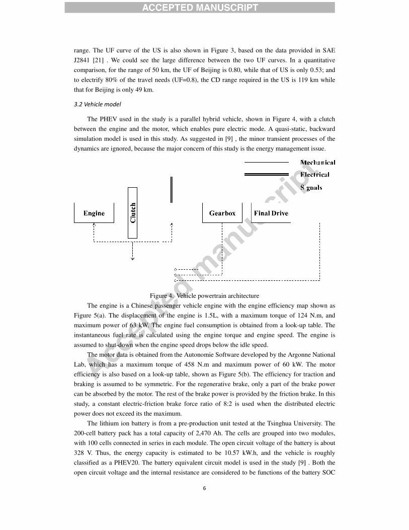
3.2 Vehicle model

The PHEV used in the study is a parallel

between the engine and the motor, which enables pure electric

simulation model is used in this

dynamics are ignored, because the major concern of this study is the energy management issue.

Figure 4.

The engine is a Chinese passenger vehicle engine

Figure 5(a). The displacement of the engine is 1.5L, with

maximum power of 63 kW. The engine

instantaneous fuel rate is calculated

assumed to shut-down when the engine speed drops below the idle speed.

The motor data is obtained from the

Lab, which has a maximum torque of 458 N.m and maximum power of 60 kW.

efficiency is also based on a look

braking is assumed to be symmetric. For the regenerative brake

can be absorbed by the motor. The rest

study, a constant electric-friction

power does not exceed its the maximum

The lithium ion battery is from

200-cell battery pack has a total capacity of 2

with 100 cells connected in series in each module. The open circuit voltage of the battery is

328 V. Thus, the energy capacity is estimated

classified as a PHEV20. The battery

open circuit voltage and the internal resistance are considered

6

range. The UF curve of the US is also shown in Figure 3, based on the data provided in SAE

. We could see the large difference between the two UF curves. In a quantitative

comparison, for the range of 50 km, the UF of Beijing is 0.80, while that of US is only 0.53; and

travel needs (UF=0.8), the CD range required in the US is 119 km while

The PHEV used in the study is a parallel hybrid vehicle, shown in Figure 4, with a clutch

between the engine and the motor, which enables pure electric mode. A quasi-static, backward

study. As suggested in [9] , the minor transient processes of the


Figure 4. Vehicle powertrain architecture

The engine is a Chinese passenger vehicle engine with the engine efficiency map shown as

The displacement of the engine is 1.5L, with a maximum torque of 124 N.m, and

The engine fuel consumption is obtained from a look-up table

calculated using the engine torque and engine speed. The engine is

down when the engine speed drops below the idle speed.

from the Autonomie Software developed by the Argonne National

maximum torque of 458 N.m and maximum power of 60 kW.

efficiency is also based on a look-up table, shown as Figure 5(b). The efficiency for traction and

symmetric. For the regenerative brake, only a part of the brake power

The rest of the brake power is provided by the friction brake.

friction brake force ratio of 8:2 is used when the distributed electric

the maximum.

The lithium ion battery is from a pre-production unit tested at the Tsinghua University.

total capacity of 2,470 Ah. The cells are grouped into two modules,

with 100 cells connected in series in each module. The open circuit voltage of the battery is

328 V. Thus, the energy capacity is estimated to be 10.57 kW.h, and the vehicle is roughly

The battery equivalent circuit model is used in the study [9]

open circuit voltage and the internal resistance are considered to be functions of the battery

sed on the data provided in SAE

difference between the two UF curves. In a quantitative

UF of Beijing is 0.80, while that of US is only 0.53; and

(UF=0.8), the CD range required in the US is 119 km while

, with a clutch

static, backward

, the minor transient processes of the


map shown as

maximum torque of 124 N.m, and

up table. The

The engine is

Argonne National

The motor

for traction and

a part of the brake power

brake power is provided by the friction brake. In this

when the distributed electric

Tsinghua University. The

to two modules,

with 100 cells connected in series in each module. The open circuit voltage of the battery is about

the vehicle is roughly

[9] . Both the

of the battery SOC

7

shown as Figure 5(c), constructed using test data.

The gearbox used in the study is an automatic with 4 speeds. The shift strategy is pre-set, and

regarded as independent from the energy management strategy. The gear shift strategy is only

related to the vehicle speed and the acceleration pedal shown as Figure 5(d).

(a) Engine map (b) Engine map

(c) Battery cell SOC feature (d) Transmission shift map

Figure 5. Component maps

The final drive ratio is 3.63. Friction loss at the final drive is ignored. The radius of the wheel

is 0.301m. Wheel slip is not considered in this study. The vehicle mass incudes the original vehicle

curb mass of 1200 kg and the battery mass of 79 kg. The fundamental vehicle longitude dynamic

equation is used to generate the vehicle speed and vehicle acceleration, shown in Equation 3. The

vehicle speed is directly read from the driving schedule.

( ) ( ) ( ) ( ) ( )t v a r g

dF t m v t F t F t F t

dt= + + + (3)

Where t is the current time, Ft is traction force required to propel the vehicle, Fa is the

aerodynamic friction, Fr is the rolling friction, Fg is the force caused by gravity when driving on

non-horizontal roads, mv is the mass of the vehicle and v is the vehicle speed.

The AECS strategy is used as the reference strategy in this study. The PHEV is assumed to

start the daily trip fully charged. With the AECS strategy, the battery energy is used exclusively

until a SOC threshold is reached. The engine is only used to make up the power gap in extreme

situations. During the CS stage, the Equivalent Consumption Minimization Strategy (ECMS) is

1000 2000 3000 4000 5000 60000

20

40

60

80

100

120

0.1

0.10.1

0.15 0.15

0.15

0.1

5

0.2

0.2

0.2

0.2

0.2

0.2

0.2

2

0.2

2

0.2

2

0.22

0.220.22

0.2

4

0.2

4

0.2

4

0.24

0.240.24

0.2

6

0.2

6

0.26 0.26

0.26

0.260.26

0.2

8

0.28

0.28

0.28

0.2

8

0.3 0.3

0.3

0.3

0.32

0.32 0.3

2

Engine Efficiency Map

Speed (r/min)

Torq

ue

(Nm

)

Engine Efficiency

Max Torque

Best Efficiency by Speed

Best Efficiency By Power

0 1000 2000 3000 4000 50000

100

200

300

400

0.7

0.7

0.7

0. 7

50

.75

0.7

5

0.8

0.8

0.8

0.8

5

0.8

5

0.8

50.85

0.9

0.9

0.9

0.9

0.9

0.9

0.9

0.9

0.9

0.9

0.9

0.9

0.9

1

0.91

0.9

1

0.91 0.91

0.91

0.9

1

0.9

1

0.9

2

0.92

0.92

0.92

0.92

0.93

0.93

0.930

.93

0.9

40.94

0.9

5

Motor Efficiency Map

Speed (r/min)

Torq

ue

(Nm

)

Motor Efficiency

Max Torque

0 0.2 0.4 0.6 0.8 13

3.1

3.2

3.3

3.4

3.5Battery Cell SOC Feature

SOC

Open C

ircuit V

oltage (

V)

0 0.2 0.4 0.6 0.8 10

0.004

0.008

0.012

0.016

0.02

Inner

Resis

tance (

ohm

)

Voltage

Resistance

0 20 40 60 80 1000

0.2

0.4

0.6

0.8

1

1.2Gearbox Shifting Strategy

Vehicle Speed (km/h)

Acc

eler

atio

n P

edal

Threshold between Gear 1 and 2



8

used to achieve near optimal fuel consumption [8] [27] . The ECMS factor is tuned for the NEDC

cycle to achieve SOC sustenance.

3.3 Optimization problem

The dynamic programming (DP) method is used to generate the solution. With DP, the global

optimal solution is obtained through backward calculation [28] . The objective function of the

optimization problem is the FCUFW. The original equation is modified as shown in Equation 4. The

cycle based equation was transformed from a distance based equation to a time based equation

with the assumption of fixed driving cycle. In addition, instead of partitioning the time horizon as

“CD + CS”, it is now partitioned as “Simulated + Un-simulated”. The very long trips are

approximated in the simulations because of their low probability of happening. For these long

range trips, it is assumed that vehicle operates in CS mode. In this study, we cover 95% of the total

trip length of all trips. For example, the length of the NEDC cycle is 10.93km. Based on the

Beijing’s UF curve, it takes 9 cycles (98.37km) to cover more than 95% of the total trip length of

all trips.

1

1

0

[( ( ) (( 1) )) ] [1 ( )]

= [( ( ) (( 1) )) ] [1 ( )]

1( ( )) ( , , ) [1 (

lastCDcycle

UFW cycle cycle CDi CDC CS

i

lastSIMcycle N

cycle cycle SIMi SIM CS

i

N T

SI

cycle

FC UF i D UF i D FC UF R FC

UF i D UF i D FC UF R FC

UFC D t m x u t dt UF RD

=

=

=

⋅

= ⋅ − − ⋅ ⋅ + − ⋅

⋅ − − ⋅ ⋅ + − ⋅

= ⋅ ⋅ + −

∑

∑

∫ � )]M CSFC⋅

(4)

Where N is the number of simulation cycles, FCSIMi is the fuel consumption in the ith

simulation cycle, RSIM is the total distance of the simulation cycles, T is the time length for each

cycle, ( , , )m x u t� is the engine fuel rate at time t, UFC(D) is the cycle utility factor at distance D

km, and the rest of the symbols have the same definitions as in Equation 1.

As the speed is directly specified by the driving cycle, the PHEV has only one degree of

freedom, which is the battery SOC (x(t)). The torque split ratio (TSR) is the control variable (u(t)).

It is defined as the motor torque divided by the total torque at the transmission input. The

dynamics can now be described by Equation 5.

2

( ) ( , , )

( ( ))- ( ( ))-4 ( ( )) ( ( ))=

2 ( ( ))

oc oc batt i

i batt

x t f x u t

V x t V x t P u t R x t

R x t Q

=�

(5)

Where x is the battery SOC, u is the torque split ratio, t is the current time, Voc is the open

circuit voltage of the battery, Pbatt is the output power of the battery, Ri is the inner resistance of

the battery and Qbatt is the capacity of the battery.

Both the control variable and the state variable are constrained. For the control variable, it

has three limits: the torque envelop curves of both engine and motor, and the power limit of the

battery. The battery is limited by the battery terminal voltage. To avoid safety hazards and rapid

degradation, the lower and upper limits of individual cells are respectively set to be 2.5 V and 3.7

V. Besides, the output power should not exceed the battery capability. For the state variable, it

must be within the SOC window (xmin, xmax). The maximum SOC is set to 0.8, and the sustaining

SOC is set to 0.3 [18] . To ensure the final SOC to be around 0.3, a penalty of SOC lower than 0.3

9

will be added to the objective function.

The optimization problem is described in Equation 6. The constant multiplier and the

“un-simulated part” in Equation 4 are omitted because they do not affect the optimization process.

A penalty function h(x) for the final SOC is added to ensure fair fuel consumption comparison.

0

min max

max

min max

min max

min : ( ( )) ( , , ) + ( ( ))

. .

( ) ( , , )

( ) ( ), { | }

0

( ) ( ) { | }

NT

eng eng

mot mot mot

batt batt batt

UFC D t m x u t dt h x NT

s t

x t f x u t

x t SOC t x x x x x

T T

u t TSR t u u T T T

U U U

⋅

=

= ∈ = ≤ ≤

≤ ≤

= ∈ = ≤ ≤

≤ ≤

∫

X

U

�

� ， (6)

Where N is the number of simulation cycles, T is the time length of each cycle, UFC(D) is

the cycle utility factor at distance D km, ( , , )m x u t� is the engine fuel rate at time t when the

battery SOC is x and the TSR is u, h(x) is the penalty function for final SOC, xmin and xmax are the

limit of battery SOC, Teng and Tmot are respectively the torques delivered by the engine and the

motor, and Ubatt is the output voltage of the battery.

In the DP optimization, the time horizon, the state space and control space are all discretized,

as shown in Figure 6. The time step is selected to be 1 second. The SOC grid is 0.001. The control

grid size is variable during the DP process, depending on the engine, motor and battery constraints.

The minimum and maximum TSR will be obtained for each grid. The admissible TSR range is

then divided into 100 sub-intervals

The Lagrangian Lk(xi, uj) for time interval k, at the state xi, with a control decision of uj is:

( , )= ( ( )) ( , )k i j k k i j

L x u UFC D t m x u t⋅ ⋅ ∆� (7)

The key feature of DP calculation is the concatenate recurrence. For the last step, there is a

final SOC penalty function. But the endpoint cost can be considered as part of the cost-to-go for

the final SOC grid. Assuming the total number of time steps is M, the optimization process at the

last time step then follows Equation 8. J*M-1(xi) is the cost-to-go at M-1 time step and ith

SOC grid.

U*M-1(xi) is the optimal control for the state grid xi at time step M-1, h(xi’) is the penalty to the

final SOC xi’, which is calculated from xM-1 and U*M-1(xi).

*

1 1 '

*

1 1 '

( ) [ ( , )+ ( )]

( ) [ ( , )+ ( )]

min

argmin

j

j

M i M i j i

u

M i M i j i

u

J x L x u h x

u x L x u h x

− −

∈

− −

∈

=

=

U

U

(8)

For time steps 1 to M-2, the process is very similar except that the endpoint penalty is

replaced by the cost-to-go function, as illustrated in Equation 9. The cost-to-go function usually

needs to be obtained through interpolation because state transition does not always fall onto a grid

point.

* *

1 '

* *

1 '

( ) [ ( , )+ ( )]

( ) [ ( , )+ ( )]

min

argmin

j

j

k i k i j k i

u

k i k i j k i

u

J x L x u J x

u x L x u J x

+

∈

+

∈

=

=

U

U

(9)

Figure 6.

The optimal control trace can be rebuilt by starting from a

specified time horizon length, by inferring the

matrix J* and u* obtained from a DP process solved using the maximum time duration.

3.4 Calculation results

Figure 7 and Figure 8 show the

utility factor of each cycle. The solid red bars indicate the cycle average fuel consumption

the AECS strategy, while the blue solid bars indicate that

shows the cycle UF. The hollow

The final FCUFW is the summation of the hollow bars, plus the

There are almost no differences between the two strategies, except for the 2

The RADOC strategy consumes

with the AECS strategy. For all other

the same. This shows that the ECMS strategy is near

AECS is nearly optimal for the given statistics

results are consistent with the analysis

strategy stays lower than that with the

consumes less fuel in the 2nd

cycle. During the CS stage, the two SOC traces share a very similar

trend, resulting in very similar fuel consumption.

10

Grids in Dynamic Programming problems

The optimal control trace can be rebuilt by starting from any user defined SOC

specified time horizon length, by inferring the optimal control and cost-to-go from the

obtained from a DP process solved using the maximum time duration.

show the calculation results. Figure 7 shows the fuel consumption and

each cycle. The solid red bars indicate the cycle average fuel consumption

rategy, while the blue solid bars indicate that using RADOC strategy. The grey curve

shows the cycle UF. The hollowed bars show the UF weighted fuel consumption of

the summation of the hollow bars, plus the weighted CS fuel consumption.

differences between the two strategies, except for the 2nd

and the 3

s more fuel in the 2nd

cycle, and less in the 3rd

cycle, compared

For all other cycles, the fuel consumptions of the two strategies are nearly

that the ECMS strategy is near-optimal for charge sustaining operation

AECS is nearly optimal for the given statistics. Figure 8 shows the corresponding

consistent with the analysis above. At the end of the 2nd

cycle, the SOC with AECS

strategy stays lower than that with the RADOC strategy, which means the AECS strategy


trend, resulting in very similar fuel consumption.

user defined SOC for any

go from the stored

shows the fuel consumption and

each cycle. The solid red bars indicate the cycle average fuel consumption using

strategy. The grey curve

each cycle.

onsumption.

and the 3rd

cycles.

cycle, compared

the two strategies are nearly

optimal for charge sustaining operations and

SOC. The

cycle, the SOC with AECS

hich means the AECS strategy


11

Figure 7. Fuel consumptions and FCUFW for each cycle

Figure 8. SOC trace comparison

As a summary, the RADOC strategy does improve the FCUFW. However, the AECS strategy

is a near-optimal strategy for PHEV20 if the vehicles are used in Beijing.

4. Scenario Analysis

In this section, scenarios with different range distributions, configurations, and driving cycles

are analyzed to verify the applicability and performance of the proposed RADOC strategy. Only

one factor changes in each scenario.

Figure 9 shows the scenario analysis diagram. The three major factors that affect fuel

economy of PHEV are: configuration, driving cycle and range distribution, shown in the top

blocks of Figure 9. The configuration diversity (varying battery sizes) will impact the ECMS

factor (also referred as SOC-to-fuel conversion factor) used in the CS stage. The range distribution

impacts the number of cycles required to cover 95% of the total trip length of all trips. The driving

cycle impacts both on the cycle number required and the ECMS factor. In the calculation of

0 1 2 3 4 5 6 7 8 9 100

0.7

1.4

2.1

2.8

3.5

4.2

4.9

5.6

6.3

7

Cycle Sequence

Fu

el

Co

nsu

mp

tio

n (

L/1

00km

)

Fuel Consumption and Utility Factor for Cycles

0 1 2 3 4 5 6 7 8 9 100

0.1

0.2

0.3

0.4

0.5

0.6

0.7

0.8

0.9

1

Cycle

Uti

lity

Facto

r

AECS / Unweighted

AECS / Weighted

RADOC / Unweighted

RADOC / Weighted

Cycle Utility Factor

0 2000 4000 6000 8000 10000 120000.2

0.3

0.4

0.5

0.6

0.7

0.8

0.9

SOC Trajectory

Time (s)

SO

C

AECS Strategy

RADOC Strategy

FCUFW (shown as Equation 4), the

number required and the ECMS factor, and the

only related to the ECMS factor.

varies, the un-simulated fuel consumption remains the same

simulated and un-simulated fuel consumptions should be re

All the results from the above blocks will

RADOC strategy and AECS strategy are compared

factor at each time, such as the configuration, driving cycle, or range di

other scenarios are obtained through the same process

compared and illustrated in the final block called

Figure 9.

4.1 Different range distribution

Four different range distributions are

RADOC strategy. The Beijing range distribution is from the survey

length distribution follows Equation

[21] . The urban logistics range distribution is based on samples from Beijing, which shows the

average daily range of a fleet of

the survey results, we created a normal distribution of

The mean value of the distribution

they travel around 200 km a day.

distribution of the taxis, where the mean

be emphasized again that the UF curve (range distribution) is different

the daily trip length distribution. The relationship between the two

As Figure 9 shows, the range distribution

number of NEDC cycles required

The fuel consumption in the “un-

because of the un-affected ECMS factor.

Simulation results for the four

12

he fuel consumption in the “simulated” part is related to both cycle

number required and the ECMS factor, and the fuel consumption in the “un-simulated” part is

Thus, in the scenario analysis, if only the cycle number required

simulated fuel consumption remains the same in all scenarios. Otherwise, both

simulated fuel consumptions should be re-calculated from scenario to scenario.

All the results from the above blocks will be gathered into the comparison block, where the

RADOC strategy and AECS strategy are compared. Then, by changing only one scenario impact

, such as the configuration, driving cycle, or range distribution, the results from

through the same process. The results of different scenarios will be

in the final block called “scenario analysis”.

Figure 9. Scenario analysis diagram

Four different range distributions are used to analyze the FCUFW improvement by

strategy. The Beijing range distribution is from the survey reported in [24]

length distribution follows Equation 2. The U.S. UF curve comes from the SAE J2841 standard

. The urban logistics range distribution is based on samples from Beijing, which shows the

a fleet of urban freight logistics trucks travels is around 100 km.

a normal distribution of the trip length for the urban logistics

of the distribution is 100 km, with a standard deviation of 5 km. For the taxi

they travel around 200 km a day. Another normal distribution is created to describe the trip length

the mean is 200 km and the standard deviation is 10 km.

the UF curve (range distribution) is different and must be derived

. The relationship between the two was reported in [25]

he range distribution only impacts the number of cycles required

required to cover 95% of the total length of all trips are shown in

-simulated” part stays the same over different range distributions,

affected ECMS factor.

for the four different range distributions show that the RADOC strategy

e “simulated” part is related to both cycle

simulated” part is

Thus, in the scenario analysis, if only the cycle number required

. Otherwise, both

calculated from scenario to scenario.

, where the

. Then, by changing only one scenario impact

stribution, the results from

. The results of different scenarios will be

improvement by the

[24] . The trip

. The U.S. UF curve comes from the SAE J2841 standard

. The urban logistics range distribution is based on samples from Beijing, which shows the

100 km. Based on

the trip length for the urban logistics case.

standard deviation of 5 km. For the taxi fleet,

to describe the trip length

10 km. It should

and must be derived from

[25] .

impacts the number of cycles required. The

trips are shown in Table 1.

simulated” part stays the same over different range distributions,

the RADOC strategy

13

improvements vary significantly, as shown in Table 1. The improvements of Beijing and US range

distributions are respectively 0.72% and 0.69%. And those of logistics and taxi range distributions

are much higher, 4.06% and 1.82%, illustrated in Figure 10. From the SOC trace comparison in

Figure 11, it is clear that the RADOC strategy is very close to the AECS strategy for the cases

with regular range distribution, e.g. Beijing and US. As the utility weighting of the fuel decreases

with the increase of trip length, the fuel consumed at short range contributes more to the FCUFW

than that at long range. As a result, the optimization chooses an AECS-like strategy, suggesting

that, for regular range distributions of relatively short trips, the electric utility is much more

important than fuel savings for the long trips. For trip populations with longer trips and less

uncertainties, such as urban logistics and taxi distributions, the RADOC strategy exhibits a

blended behavior. In these distributions, the range is very likely longer than the AER. This results

in equal utility weightings for the fuel consumption within that distance, which is illustrated as a

straight UF curve shown in Figure 11, where the slope shows the cycle UF weighting.

In summary, for regular range distributions, the RADOC strategy can be approximated by a

simple AECS strategy to achieve minimum FCUFW; for special range distributions with less

uncertainty, such as the logistics and taxi fleets, the RADOC strategy will be implemented as a

blended strategy.

Table 1. Results of different range distributions

Beijing US Logistics Taxi

Cycles required 9 29 9 18

AECS (L/100km) 2.24 3.37 3.74 4.41

RADOC (L/100km) 2.22 3.35 3.59 4.33

Improvement 0.72% 0.69% 4.07% 1.82%

Figure 10. FCUFW comparison of different range distributions

Beijing U.S. Logistics Taxi0

0.6

1.2

1.8

2.4

3

3.6

4.2

4.8

5.4

6

Range Distributions

Fu

el

Co

nsu

mp

tio

n (

L/1

00km

)

Fuel Consumption Improvement by RADOC over different distributions

Beijing U.S. Logistics Taxi0

0.6

1.2

1.8

2.4

3

3.6

4.2

4.8

5.4

6

Fu

el

Co

nsu

mp

tio

n I

mp

rovem

en

t (%

)

Fuel Consumption of AECS

Fuel Consumption of RADOC

Fuel Consumption Improvement by RADOC

14

Figure 11. SOC and UF curve comparisons of different range distributions

4.2 Different configuration

Three different configurations, including PHEV10, PHEV20, and PHEV40, are used to

analyze the FCUFW improvement by the RADOC strategy. The only difference between the

configurations is the battery size. With the same battery cell model and the same module

consisting of 100 cells in series, the PHEV10 has only one module, PHEV20 has two modules

connected in parallel, and PHEV40 has four modules connected in parallel. As a result of the

arrangement, the nominal open circuit voltages of the three configurations are the same.

The configuration diversity (varying battery sizes) causes the difference in ECMS factor

shown as Figure 9. So, the fuel consumptions for both “simulated” and “un-simulated” parts

should be re-calculated for every configuration.

The final results are shown in Table 2 and Figure 12. There is an obvious trend that the

improvement by RADOC strategy increases with the decrease of battery installed in the PHEV.

For PHEV40, the SOC traces with two strategies almost duplicate each other shown in Figure 13.

But for PHEV10, the two traces are apart from each other. This results coincide with the strategies

in the product PHEVs. For Prius PHV, it operates in blended mode before the charge is depleted

[29] . But for Chevy Volt, it is a typical range extend vehicle, which means it operates exactly as

0 50 100 150 200 250 300 3500.2

0.4

0.6

0.8

1

SOC Trajectories

Distance (km)

SO

C

RADOC Solution of Beijing

RADOC Solution of US

RADOC Solution of Logistics

RADOC Solution of Taxi

AECS for All

0 50 100 150 200 250 300 3500

0.2

0.4

0.6

0.8

1

1.2

1.4Utility Factor Curve

Distance (km)

Uti

lity

Facto

r

Beijing

U.S.

Logistics

Taxi

15

an EV whenever there is available electric energy. Speaking of the reason, the electric power from

PHEV10 is not large enough to propel the vehicle for some portion of the driving cycle. With the

AECS strategy, the engine only supplements the power gap between the demand and the motor.

Usually, it is not efficient to do so if the power gap indicates a low load to the engine. Instead, the

RADOC strategy will optimally reserve some electricity for this portion of cycle, and distribute a

high load to the engine as the engine has to start anyway. This results in a blended use of both

electricity and fuel before the CS stage in PHEV10.

As a summary, the RADOC strategy benefits the PHEV with small battery by offering an

appropriate blended, regarding the driving range distribution.

Table 2. Results of different configurations

PHEV10 PHEV20 PHEV40

Cells in total 100 200 400

Cells in series 100 100 100

Modules in parallel 1 2 4

ECMS factor (kg) -1.02 -2.06 -4.12

CS Fuel Consumption

(L/100km) 5.13 5.09 5.15

AECS (L/100km) 3.59 2.24 0.89

RADOC (L/100km) 3.47 2.22 0.88

Improvement 3.30% 0.72% 0.26%

Figure 12. FCUFW comparison of different configurations


0.5

1

1.5

2

2.5

3

3.5

4

4.5

5

Configurations

Fu

el

Co

nsu

mp

tio

n (

L/1

00km

)

Fuel Consumption Improvement by RADOC over different configurations


0.4

0.8

1.2

1.6

2

2.4

2.8

3.2

3.6

4

Fu

el

Co

nsu

mp

tio

n I

mp

rovem

en

t (%

)




16

Figure 13. SOC comparison of different configurations

4.3 Different driving cycles

Three different driving cycles are included in this analysis. The NEDC cycle used in the base

case is regarded as a combined cycle of urban and highway driving. The UDDS cycle is a typical

urban driving cycle, while the HFEDS cycle represents the typical highway driving cycle.

As the shown in Figure 9, the driving cycle impacts both on the cycle number required and

the ECMS strategy for the CS stage. Thus, in the calculation of FCUFW, the fuel consumptions of

both “simulated” and “un-simulated” parts are different from cycle to cycle.

The analysis result shows that, the improvements brought by RADOC strategy over AECS

strategy are all very small – below 1%, shown in Table 3 and Figure 14. The improvement of the

highway driving cycles are higher than that of the urban driving cycle. The SOC trace comparison

in Figure 15 shows the difference. For highway driving cycles, there is an obvious blended

interval before the charge is completed depleted. The SOC trend verifies the conceptual sketches

of this study, shown in Figure 2. For the urban driving cycle, the SOC traces with two strategies

almost duplicate, so that the FCUFWs are very close. The SOC trend of the combined driving cycle

shows the trend in between the two above, as expected. Because in the blended operations, the

engine starts to propel the vehicle in cooperating with the motor. For most of the engines, the

efficiency at a high load is better than that at a low load. This is why the more highway driving

takes the proportion in a cycle, the more blended the RADOC strategy prefers.

As a summary, although the RADOC strategy is very close to the AECS strategy with all

driving cycles, the RADOC strategy works more effectively for highway cycles than for urban

cycles.

0 10 20 30 40 50 60 70 80 90 1000.2

0.3

0.4

0.5

0.6

0.7

0.8

0.9SOC Trajectories

Distance (km)

SO

C

RADOC PHEV10

RADOC PHEV20

RADOC PHEV40

AECS PHEV10

AECS PHEV20

AECS PHEV40

17

Table 3. Results of different driving cycles

NEDC UDDS HFEDS

Cycle range (km) 10.93 11.99 16.51

Range coverage 0.95

Cycles required 9 8 6

ECMS factor(kg) -2.06 -2.07 -1.96

CS Fuel Consumption (L/100km) 5.09 3.87 6.08

AECS (L/100km) 2.24 1.22 3.13

RADOC (L/100km) 2.22 1.22 3.11

Improvement 0.72% 0.10% 0.66%

Figure 14. FCUFW comparison of different driving cycles

NEDC UDDS HFEDS0

0.4

0.8

1.2

1.6

2

2.4

2.8

3.2

3.6

4

Driving cycles

Fu

el

Co

nsu

mp

tio

n (

L/1

00km

)

Fuel Consumption Improvement by RADOC over different driving cycles

NEDC UDDS HFEDS0

0.1

0.2

0.3

0.4

0.5

0.6

0.7

0.8

0.9

1

Fu

el

Co

nsu

mp

tio

n I

mp

rovem

en

t (%

)




18

Figure 15. SOC comparison of different driving cycles

5. Conclusion

This paper proposes a range adaptive optimal control strategy which minimizes the utility

factor weighted fuel consumption (FCUFW). The contributions are summarized as following:

(1) This research proposes a novel idea of minimizing the FCUFW in energy management

strategy development for PHEVs, as it is a significant factor to evaluate the average fuel

consumption of PHEV considering the utility intensity.

(2) The range adaptive optimal control (RADOC) strategy is developed by dynamic

programming (DP) to achieve the objective of minimizing the FCUFW, and it is verified to be

available in different scenarios.

(3) According to the scenario analysis: The RADOC strategy can be replaced with AECS

strategy when the PHEV is used in regular daily use, while it can be replaced with blended

strategy when the PHEV is used as an urban logistics vehicle or a taxi; the RADOC strategy

improves more for the PHEV with small batteries than for that with large batteries; and, the

RADOC strategy works more effectively in highway driving than in urban driving.

This paper has just verified the necessity of the RADOC strategy via DP. The real-time

implementation of RADOC strategy will be studied in the future. After that, the RADOC strategy

will be combined with the earlier developed A-PMP strategy [30] to respectively deal with the

cases of unknown and known trip length. When the combined strategy is applied to the vehicle,

the fuel consumption will be optimized no matter whether the driver inputs the trip length before a

trip. If the trip length is given by the driver, the A-PMP strategy will be applied to offer the

0 10 20 30 40 50 60 70 80 90 1000.2

0.3

0.4

0.5

0.6

0.7

0.8

0.9

SOC Trajectories

Distance (km)

SO

C

RADOC NEDC

RADOC UDDS

RADOC HFEDS

AECS NEDC

AECS UDDS

AECS HFEDS

19

minimum fuel consumption for the coming trip; otherwise, the RADOC strategy will be applied to

minimize the FCUFW based on the historical trip statistics of the driver.

Acknowledgement

The collaboration is made possible under the US-China Clean Energy Research Center, a

joint center sponsored by China MOST and US DOE. This work is funded by the NSFC (National

Natural Science Foundation) of China under the contract of No. 61004075, and the MOST

(Ministry of Science and Technology) of China under the contracts of No. 2013BAG16B01 and

No. 2010DFA72760.

Reference

[1] Guang Wu, Xing Zhang, Zuomin Dong, Powertrain architectures of electrified vehicles:

review, classification and comparison, Journal of the Franklin Institute,

http://dx.doi.org/10.1016/j.jfranklin.2014.04.018

[2] Toyota Prius PHV specifications, http://www.toyota.com/prius-plug-in/#!/Welcome,

2013.10.20

[3] GM Chevy volt specifications, http://www.chevrolet.com/volt-electric-car.html, 2013.10.20

[4] Ford C-max energi speficifcations, http://www.ford.com/cars/cmax/trim/energi/, 2013.10.20

[5] Gong, Qiuming, Yaoyu Li, and Zhong-Ren Peng. "Optimal power management of plug-in

HEV with intelligent transportation system." Advanced intelligent mechatronics, 2007

IEEE/ASME international conference on. IEEE, 2007.

[6] Honarmand, Masoud, Alireza Zakariazadeh, and Shahram Jadid. "Self-scheduling of electric

vehicles in an intelligent parking lot using stochastic optimization." Journal of the Franklin

Institute (2014). http://dx.doi.org/10.1016/j.jfranklin.2014.01.019

[7] Sanjaka G. Wirasingha, Ali Emadi, Classification and Review of Control Strategies for

Plug-In Hybrid Electric Vehicles, IEEE Transaction on vehicular technology, VOL. 60, NO. 1,

JANUARY 2011, 111-122

[8] Serrao, Lorenzo. A comparative analysis of energy management strategies for hybrid electric

vehicles. Diss. Ohio State University, 2009.

[9] Guzzella, Lino, and Antonio Sciarretta. Vehicle propulsion systems. Springer, 2007.

[10] Banvait, Harpreetsingh, Sohel Anwar, and Yaobin Chen. A rule-based energy management

strategy for plug-in hybrid electric vehicle (PHEV). In American Control Conference, 2009.

ACC'09., pp. 3938-3943. IEEE, 2009.

[11] Montazeri-Gh, Morteza, Amir Poursamad, and Babak Ghalichi. Application of genetic

algorithm for optimization of control strategy in parallel hybrid electric vehicles. Journal of

the Franklin Institute 343.4 (2006): 420-435.

[12] Cong HOU, Minggao OUYANG, Hewu WANG, Liangfei XU, An assessment of PHEV

energy management strategies using driving range data collected in Beijing, EVS27

International Battery, Hybrid and Fuel Cell Electric Vehicle Symposium, NOV, 2013.

[13] Kum, Dongsuk, Huei Peng, and Norman Bucknor. Optimal control of plug-in HEVs for fuel

economy under various travel distances. Advances in Automotive Control. 2010.

[14] Karbowski, Dominik, S. Pagerit, J. Kwon, A. Rousseau, and K. Pechmann. Fair comparison

20

of powertrain configurations for plug-in hybrid operation using global optimization. In SAE

World Congress, Detroit SAE paper, pp. 01-1334. 2009.

[15] Lai L, Ehsani M. Dynamic Programming Optimized Constrained Engine on and off

Control Strategy for Parallel HEV[C]//Vehicle Power and Propulsion Conference (VPPC),

2013 IEEE. IEEE, 2013: 1-5.

[16] Kim, Namwook, Sukwon Cha, and Huei Peng. Optimal control of hybrid electric

vehicles based on Pontryagin's minimum principle. Control Systems Technology, IEEE

Transactions on 19.5 (2011): 1279-1287.

[17] Kim, Namwook, Aymeric Rousseau, and Daeheung Lee. A jump condition of

PMP-based control for PHEVs. Journal of Power Sources 196.23 (2011): 10380-10386.

[18] Gong, Qiuming, Yaoyu Li, and Zhong-Ren Peng. Trip based power management of

plug-in hybrid electric vehicle with two-scale dynamic programming. Vehicle Power and

Propulsion Conference, 2007. VPPC 2007. IEEE. IEEE, 2007.

[19] Kum, Dongsuk, Huei Peng, and Norman K. Bucknor. "Optimal energy and catalyst

temperature management of plug-in hybrid electric vehicles for minimum fuel consumption

and tail-pipe emissions." Control Systems Technology, IEEE Transactions on 21.1 (2013):

14-26.

[20] Duoba, Michael. Evaluating PHEV technology using component HIL, subsystem, and

chassis dynamometer testing: methods and results. SAE Hybrid Vehicle Technologies 2007

Symposium. 2007.

[21] SAE International, Utility Factor Definitions for Plug-In Hybrid Electric Vehicles Using

2001 U.S. DOT National Household Travel Survey Data. SAE J2841 [S] MAR, 2009.

[22] National Household Travel Survey official website, http://nhts.ornl.gov/, 2013.10.20

[23] SAE International, Recommended Practice for Measuring the Exhaust Emissions and

Fuel Economy of Hybrid-Electric Vehicles, Including Plug-in Hybrid Vehicles SAE J1711 [S]

JUN, 2010.

[24] Lvwei Wu, A GPS-based Research on the Driving Patterns of Private Passenger Vehicle

in Beijing. Diss. Tsinghua University, 2013.

[25] Xing Zhang, Guang Wu, Zuomin Dong, Curran Crawford, Embedded feature-selection

support vector machine for driving pattern recognition, Journal of the Franklin Institute,

http://dx.doi.org/10.1016/j.jfranklin.2014.04.021

[26] Cong Hou, Hewu Wang & Minggao Ouyang, A methodology of calculating PHEV

average fuel consumption based on the trip range distribution, Automotive Engineering, In

Press, 2013.

[27] Sciarretta, Antonio, and Lino Guzzella. Control of hybrid electric vehicles. Control

systems, IEEE 27.2 (2007): 60-70.

[28] Kirk, Donald E. Optimal control theory: an introduction. DoverPublications. com, 2012.

[29] Carlson, Richard W., Michael J. Duoba, Theodore P. Bohn, and Anantray D. Vyas ,

Testing and analysis of three plug-in hybrid electric vehicles. SAE International, 2007.

[30] Hou, Cong, Ouyang, Minggao, Xu, Liangfei, and Wang Hewu. Approximate Pontryagin’s

minimum principle applied to the energy management of plug-in hybrid electric vehicles. Applied

Energy 115 (2014): 174-189.

21

Table 4. Results of different range distributions

Beijing US Logistics Taxi

Cycles required 9 29 9 18

AECS (L/100km) 2.24 3.37 3.74 4.41

RADOC (L/100km) 2.22 3.35 3.59 4.33

Improvement 0.72% 0.69% 4.07% 1.82%

Table 5. Results of different configurations


Cells in total 100 200 400

Cells in series 100 100 100

Modules in parallel 1 2 4

ECMS factor (kg) -1.02 -2.06 -4.12

CS Fuel Consumption

(L/100km) 5.13 5.09 5.15

AECS (L/100km) 3.59 2.24 0.89

RADOC (L/100km) 3.47 2.22 0.88

Improvement 3.30% 0.72% 0.26%

Table 6. Results of different driving cycles

NEDC UDDS HFEDS

Cycle range (km) 10.93 11.99 16.51

Range coverage 0.95

Cycles required 9 8 6

ECMS factor(kg) -2.06 -2.07 -1.96

CS Fuel Consumption (L/100km) 5.09 3.87 6.08

AECS (L/100km) 2.24 1.22 3.13

RADOC (L/100km) 2.22 1.22 3.11

Improvement 0.72% 0.10% 0.66%

� An optimal PHEV energy management strategy minimizing utility factor weighted fuel

consumption

� An adaptive optimal control strategy based on travel statistics

� AECS strategy, a good choice for regular daily use

� Blended strategy, a good choice for logistics vehicle and taxi

author's accepted manuscript - tsinghua university · vehicles with unknown trip length cong...

Documents