Essays on the Analysis of High-Dimensional Dynamic Games and Data Combination

By

Carlos Andrew Manzanares

Dissertation

Submitted to the Faculty of the

Graduate School of Vanderbilt University

in partial fulfillment of the requirements

for the degree of

DOCTOR OF PHILOSOPHY

in

Economics

August, 2016

Nashville, Tennessee

Approved by:

Tong Li

Yanqin Fan

Andrea Moro

Alejandro Molnar

Patrick L. Bajari

ACKNOWLEDGMENTS

I thank Tong Li for graciously serving as my co-advisor. I also thank my co-advisor Yanqin Fan, whose men-

torship and tireless concern on my behalf have played a central role in my formation as a scholar. Additionally, I

thank Patrick Bajari for his extensive and conscientious advising and professional support, which far exceeded his

formal role as a dissertation committee member. I also thank my dissertation committee members Andrea Moro

and Alejandro Molnar for their invaluable contributions of time, insight, and advice. I thank the Departments of

Economics at Vanderbilt University and the University of Washington for coordinating an extensive and rewarding

visit to the University of Washington, as well as the eScience Institute at the University of Washington (especially,

Bill Howe and Andrew Whitaker), which introduced me to cloud computing and connected me to the broader data

science community. This experience greatly enhanced my research program. My research has benefited considerably

from conversations with Benito Arrunada, Gregory Duncan, Martin Gaynor, Panle Jia, Phillip Leslie, Chris Nosko,

Alberto Abadie, Valentina Staneva, Rahul Biswas, Charles Romeo, Fahad Khalil, Yu-chin Chen, Andrew Daughety,

Jennifer Reinganum, Gregory Leo, Federico Gutierrez, Irene Botosaru, and others too numerous to mention. Funding

from the National Science Foundation, Vanderbilt University, and the Mercatus Center, as well as an internship at

Amazon, are gratefully acknowledged.

To my parents, Carlos and Deborah, I thank you for your unwavering love, support, and encouragement and for

being the best role models and mentors I could hope for. To Christina, I thank you for being my best friend and for

sharing these experiences with me daily. To Chris, I thank you for being the best brother anyone could ask for, for

always being with us in spirit, and for watching over us. We love you and miss you everyday. Finally, I thank and

praise my Lord and Savior Jesus Christ for allowing me to draw upon His faithfulness and strength throughout this

journey.

ii

TABLE OF CONTENTS

Chapter Page

ACKNOWLEDGMENTS . . . . . . . . . . . . . . . . . . . . . . . . . . . . . . . . . . . . . . . . . . . . . . ii

LIST OF TABLES . . . . . . . . . . . . . . . . . . . . . . . . . . . . . . . . . . . . . . . . . . . . . . . . . v

LIST OF FIGURES . . . . . . . . . . . . . . . . . . . . . . . . . . . . . . . . . . . . . . . . . . . . . . . . . vii

1 New Entry and Mergers in Network Industries: Evidence from U.S. Airlines . . . . . . . . . . . . . . . . 1

1.1 Background . . . . . . . . . . . . . . . . . . . . . . . . . . . . . . . . . . . . . . . . . . . . . . . . 71.2 Model . . . . . . . . . . . . . . . . . . . . . . . . . . . . . . . . . . . . . . . . . . . . . . . . . . . 11

1.2.1 Preliminaries . . . . . . . . . . . . . . . . . . . . . . . . . . . . . . . . . . . . . . . . . . . 121.2.2 Network-Wide Capacity Game . . . . . . . . . . . . . . . . . . . . . . . . . . . . . . . . . 121.2.3 Price Competition . . . . . . . . . . . . . . . . . . . . . . . . . . . . . . . . . . . . . . . . 18

1.3 Data . . . . . . . . . . . . . . . . . . . . . . . . . . . . . . . . . . . . . . . . . . . . . . . . . . . . 221.3.1 Sources . . . . . . . . . . . . . . . . . . . . . . . . . . . . . . . . . . . . . . . . . . . . . . 221.3.2 Sample Selection . . . . . . . . . . . . . . . . . . . . . . . . . . . . . . . . . . . . . . . . . 231.3.3 Data Summary . . . . . . . . . . . . . . . . . . . . . . . . . . . . . . . . . . . . . . . . . . 24

1.4 Identification and Estimation . . . . . . . . . . . . . . . . . . . . . . . . . . . . . . . . . . . . . . . 271.4.1 Overview . . . . . . . . . . . . . . . . . . . . . . . . . . . . . . . . . . . . . . . . . . . . . 271.4.2 First Stage: Profits and Strategies . . . . . . . . . . . . . . . . . . . . . . . . . . . . . . . . 30

1.4.3 Second Stage: Capacity Game . . . . . . . . . . . . . . . . . . . . . . . . . . . . . . . . . . 33

1.5 Results . . . . . . . . . . . . . . . . . . . . . . . . . . . . . . . . . . . . . . . . . . . . . . . . . . 401.5.1 Model Estimates . . . . . . . . . . . . . . . . . . . . . . . . . . . . . . . . . . . . . . . . . 401.5.2 Value of Defense . . . . . . . . . . . . . . . . . . . . . . . . . . . . . . . . . . . . . . . . . 48

1.6 Conclusion . . . . . . . . . . . . . . . . . . . . . . . . . . . . . . . . . . . . . . . . . . . . . . . . 54

2 Improving Policy Functions in High-Dimensional Dynamic Games . . . . . . . . . . . . . . . . . . . . . 56

2.1 Method Characterization . . . . . . . . . . . . . . . . . . . . . . . . . . . . . . . . . . . . . . . . . 602.1.1 Model . . . . . . . . . . . . . . . . . . . . . . . . . . . . . . . . . . . . . . . . . . . . . . 602.1.2 Policy Function Improvement . . . . . . . . . . . . . . . . . . . . . . . . . . . . . . . 65

2.2 Empirical Illustration . . . . . . . . . . . . . . . . . . . . . . . . . . . . . . . . . . . . . . . . . . . 722.2.1 Institutional Background and Data . . . . . . . . . . . . . . . . . . . . . . . . . . . . . . . 722.2.2 Model Adaptation . . . . . . . . . . . . . . . . . . . . . . . . . . . . . . . . . . . . . . . . 732.2.3 Policy Function Improvement . . . . . . . . . . . . . . . . . . . . . . . . . . . . . . . . . . 76

2.2.4 Results . . . . . . . . . . . . . . . . . . . . . . . . . . . . . . . . . . . . . . . . . . . . . . 782.3 Conclusion . . . . . . . . . . . . . . . . . . . . . . . . . . . . . . . . . . . . . . . . . . . . . . . . 86

3 Partial Identification of Average Treatment Effects on the Treated via Difference-in-Differences . . . . . . 89

3.1 Partial Identification of the Average Treatment Effect on the Treated . . . . . . . . . . . . . . . . . . 913.1.1 Sharp bounds on AT T (x) and AT T . . . . . . . . . . . . . . . . . . . . . . . . . . . . . . . 923.1.2 A Numerical Example . . . . . . . . . . . . . . . . . . . . . . . . . . . . . . . . . . . . . . 95

3.2 Identification of AT T (x) and AT T Under An Exclusion Restriction . . . . . . . . . . . . . . . . . . . 973.3 Bounds on AT T (x) and AT T When a Matched Subsample is Available . . . . . . . . . . . . . . . . . 100

3.3.1 Identification of AT T (x) and AT T When Matched Sample is Random . . . . . . . . . . . . . 1023.3.2 Sharp Bounds on AT T (x) and AT T When Sampling Procedure for Matched Sample is Un-

known . . . . . . . . . . . . . . . . . . . . . . . . . . . . . . . . . . . . . . . . . . . . . . 1033.4 An Empirical Application . . . . . . . . . . . . . . . . . . . . . . . . . . . . . . . . . . . . . . . . . 104

3.4.1 Estimation . . . . . . . . . . . . . . . . . . . . . . . . . . . . . . . . . . . . . . . . . . . . 1053.4.2 Results . . . . . . . . . . . . . . . . . . . . . . . . . . . . . . . . . . . . . . . . . . . . . . 108

3.5 Conclusion . . . . . . . . . . . . . . . . . . . . . . . . . . . . . . . . . . . . . . . . . . . . . . . . 109

iii

BIBLIOGRAPHY . . . . . . . . . . . . . . . . . . . . . . . . . . . . . . . . . . . . . . . . . . . . . . . . . 110

A Chapter 1 Appendix . . . . . . . . . . . . . . . . . . . . . . . . . . . . . . . . . . . . . . . . . . . . . . 116

A.1 Supplemental Tables . . . . . . . . . . . . . . . . . . . . . . . . . . . . . . . . . . . . . . . . . . . 116A.2 Estimation Details . . . . . . . . . . . . . . . . . . . . . . . . . . . . . . . . . . . . . . . . . . . . 121

A.2.1 First Stage: Demand Estimation . . . . . . . . . . . . . . . . . . . . . . . . . . . . . . . . . 121A.2.2 First Stage: Marginal Costs . . . . . . . . . . . . . . . . . . . . . . . . . . . . . . . . . . . 123

A.3 Miscellaneous . . . . . . . . . . . . . . . . . . . . . . . . . . . . . . . . . . . . . . . . . . . . . . 124A.3.1 Low Cost Carrier List . . . . . . . . . . . . . . . . . . . . . . . . . . . . . . . . . . . 124A.3.2 Original Input Model Specification . . . . . . . . . . . . . . . . . . . . . . . . . . . . . . . 124

A.4 Ongoing and Future Work . . . . . . . . . . . . . . . . . . . . . . . . . . . . . . . . . . . . . . . . 130A.4.1 Summary . . . . . . . . . . . . . . . . . . . . . . . . . . . . . . . . . . . . . . . . . . . . 130A.4.2 Fixed, Entry, and Exit Costs . . . . . . . . . . . . . . . . . . . . . . . . . . . . . . . . . . . 131

B Chapter 2 Appendix . . . . . . . . . . . . . . . . . . . . . . . . . . . . . . . . . . . . . . . . . . . . . . 132

B.1 Supplemental Tables . . . . . . . . . . . . . . . . . . . . . . . . . . . . . . . . . . . . . . . . . . . 132B.1.1 Section 2.2.1 Tables . . . . . . . . . . . . . . . . . . . . . . . . . . . . . . . . . . . . . . . 132B.1.2 Section 2.2.2 Tables . . . . . . . . . . . . . . . . . . . . . . . . . . . . . . . . . . . . . . . 133B.1.3 Section 2.2.4 Table . . . . . . . . . . . . . . . . . . . . . . . . . . . . . . . . . . . . . . . . 135

B.2 Section Details . . . . . . . . . . . . . . . . . . . . . . . . . . . . . . . . . . . . . . . . . . . . . . 137B.2.1 Section 2.2.1 Details . . . . . . . . . . . . . . . . . . . . . . . . . . . . . . . . . . . . . . . 137B.2.2 Section 2.2.2 Details . . . . . . . . . . . . . . . . . . . . . . . . . . . . . . . . . . . . . . 137B.2.3 Section 2.2.4 Details . . . . . . . . . . . . . . . . . . . . . . . . . . . . . . . . . . . . . . . 141

C Chapter 3 Appendix . . . . . . . . . . . . . . . . . . . . . . . . . . . . . . . . . . . . . . . . . . . . . . 142

iv

LIST OF TABLES

1.1 Legacy Carrier and Low Cost Carrier Flight Capacity Increases and Decreases by Merger, Proportionof Markets . . . . . . . . . . . . . . . . . . . . . . . . . . . . . . . . . . . . . . . . . . . . . . . . . 11

1.2 Price Competition Variables Summary . . . . . . . . . . . . . . . . . . . . . . . . . . . . . . . . . . 26

1.3 Entry and Capacity Variables Summary . . . . . . . . . . . . . . . . . . . . . . . . . . . . . . . . . 27

1.4 Estimated Demand and Marginal Cost Models (Two Stage GMM), 2008q1 - 2008q3 . . . . . . . . . 41

1.5 Estimated Reduced-Form Profit Models, 2008q1 - 2008q3 . . . . . . . . . . . . . . . . . . . . . . . 43

1.6 Estimated Entry and Capacity Strategies . . . . . . . . . . . . . . . . . . . . . . . . . . . . . . . . . 45

1.7 Estimated Choice-Specific Value of Flight Capacity (Boosted Regression): Delta Airlines, 2008q2 . . 46

1.8 Estimated Choice-Specific Value of Flight Capacity (Boosted Regression): Northwest Airlines, 2008q2 47

1.9 Estimated Choice-Specific Value of Flight Capacity (Boosted Regression): Delta and NorthwestMerged, 2008q2 . . . . . . . . . . . . . . . . . . . . . . . . . . . . . . . . . . . . . . . . . . . . . . 47

1.10 Profitability of Offering 280 flights From Chicago to MSP, 2008q2, Southwest Airlines (Millions ofUS $) . . . . . . . . . . . . . . . . . . . . . . . . . . . . . . . . . . . . . . . . . . . . . . . . . . . 49

1.11 Change in Value of Defending Chicago to MSP Against Southwest Entry, Delta and Northwest, Pre-to Post-Merger . . . . . . . . . . . . . . . . . . . . . . . . . . . . . . . . . . . . . . . . . . . . . . 49

1.12 Southwest Unentered Segments in 2008q1 . . . . . . . . . . . . . . . . . . . . . . . . . . . . . . . . 51

1.13 Value of Defense (Median and Mean) . . . . . . . . . . . . . . . . . . . . . . . . . . . . . . . . . . 51

1.14 Merger-Induced Changes in Characteristics Affecting Profitability (Delta and Northwest Merger,2008q2 Data) . . . . . . . . . . . . . . . . . . . . . . . . . . . . . . . . . . . . . . . . . . . . . . . 53

2.1 Estimated Choice-Specific Value Function Models (Boosted Regression), Baseline Specification . . . 79

2.2 Simulation Results by Specification (Per-Store Average) . . . . . . . . . . . . . . . . . . . . . . . . 82

2.3 Simulation Results by Merchandise Type (Baseline Specification, Per-Store Average) . . . . . . . . . 84

3.1 Comparison of Botosaru and Gutierrez (2015) to Fan and Manzanares (2016) . . . . . . . . . . . . . 100

3.2 Data Summary . . . . . . . . . . . . . . . . . . . . . . . . . . . . . . . . . . . . . . . . . . . . . . 104

3.3 Empirical Application Results . . . . . . . . . . . . . . . . . . . . . . . . . . . . . . . . . . . . . . 108

v

A.1 Timeline of Merger Events . . . . . . . . . . . . . . . . . . . . . . . . . . . . . . . . . . . . . . . . 116

A.3 Distribution Summary, Value of Defense . . . . . . . . . . . . . . . . . . . . . . . . . . . . . . . . . 116

A.2 List of Southwest Flight Segments Unentered in 2008q1 . . . . . . . . . . . . . . . . . . . . . . . . 117

A.4 CSA Airport Correspondences . . . . . . . . . . . . . . . . . . . . . . . . . . . . . . . . . . . . . . 118

A.5 Estimated Choice-Specific Value of Flight Capacity (Boosted Regression): Delta Airlines, 2008q2(Full Set of Regressors) . . . . . . . . . . . . . . . . . . . . . . . . . . . . . . . . . . . . . . . . . . 119

A.6 Estimated Choice-Specific Value of Flight Capacity (Boosted Regression): Northwest Airlines, 2008q2(Full Set of Regressors) . . . . . . . . . . . . . . . . . . . . . . . . . . . . . . . . . . . . . . . . . . 120

A.7 Estimated Choice-Specific Value of Flight Capacity (Boosted Regression): Delta and NorthwestMerged, 2008q2 (Full Set of Regressors) . . . . . . . . . . . . . . . . . . . . . . . . . . . . . . . . . 121

A.8 List of Hubs . . . . . . . . . . . . . . . . . . . . . . . . . . . . . . . . . . . . . . . . . . . . . . . . 121

A.9 Estimated Demand and Marginal Cost Models (First Stage GMM), 2006q1 . . . . . . . . . . . . . . 126

A.10 Estimated Reduced-Form Profit Models (Original Specification), 2008q1 - 2008q3 . . . . . . . . . . 127

A.11 Estimated Entry and Capacity Strategies (Original Specification) . . . . . . . . . . . . . . . . . . . . 129

B.1 General Merchandise Distribution Centers . . . . . . . . . . . . . . . . . . . . . . . . . . . . . . . . 132

B.2 Food Distribution Centers . . . . . . . . . . . . . . . . . . . . . . . . . . . . . . . . . . . . . . . . . 133

B.3 State Space Cardinality Calculation . . . . . . . . . . . . . . . . . . . . . . . . . . . . . . . . . . . 134

B.4 Parameter Values by Specification . . . . . . . . . . . . . . . . . . . . . . . . . . . . . . . . . . . . 135

B.5 Estimated Choice-Specific Value Function Models (OLS), Baseline Specification . . . . . . . . . . . 136

vi

LIST OF FIGURES

1.1 Low Cost Carrier Share of Passengers, Delta and Northwest Hubs . . . . . . . . . . . . . . . . . . . 10

1.2 Probability of Southwest Entry and the Mean Value of Defense Change, Pre- to Post-Merger, Deltaand Northwest . . . . . . . . . . . . . . . . . . . . . . . . . . . . . . . . . . . . . . . . . . . . . . 52

2.1 Wal-Mart Distribution Center and Store Diffusion Map (1962 to 2006) . . . . . . . . . . . . . . . . 74

2.2 Simulation Results, Representative Simulation (2000 to 2006) . . . . . . . . . . . . . . . . . . . . . 86

2.3 Multi-Step Policy Improvement . . . . . . . . . . . . . . . . . . . . . . . . . . . . . . . . . . . . . 87

3.1 Relationship Between ρ and θ Given p . . . . . . . . . . . . . . . . . . . . . . . . . . . . . . . . . 96

vii

Chapter 1

New Entry and Mergers in Network Industries: Evidence from U.S. Airlines

From 1994 to 2007, prior to its merger with Delta Airlines in 2008, Northwest Airlines accounted for seventy-

four percent of passenger enplanements from the Minneapolis-St. Paul (MSP) airport, on average. To protect its

dominant position, Northwest typically responded to new low cost carrier entrants with aggressive price drops and

increases in the number of offered flights, with several of these responses generating allegations of predatory pricing

and antitrust scrutiny.1 Not surprisingly, low cost carriers maintained a relatively small presence at MSP, accounting

for an average of five percent of passenger enplanements from the airport from 1995 to 2007.2 With a small share of

low cost carrier flights, fares through MSP remained relatively high, consistently ranking as some of the highest fares

among major U.S. domestic airports during the same time period.3

In the second quarter of 2008, Northwest announced its merger with Delta. Almost immediately after this an-

nouncement, Southwest Airlines, the dominant low cost carrier in the United States, declared its intentions to offer

nonstop flights from MSP to Chicago, which represented its first regular nonstop flight offerings from MSP. South-

west’s entry initiated a wave of low cost carrier flight offerings, with so many new offerings that the governing

authorities at MSP expanded the airport to accommodate the growing presence of low cost carriers, whose share of

enplaned passengers increased to an all-time high of nineteen percent in 2014.4

What would drive a dominant incumbent with a history of aggressively responding to new entrants to seemingly

give up this competitive position and accommodate entry after a merger? This paper answers this question. Existing

models of predatory behavior might conclude that Northwest would become more likely to defend MSP against new

entrants after the merger. For example, ”long purse/deep pockets” predation models argue that predatory pricing

1 For an extensive analysis of the predatory pricing practices of Northwest Airlines at the Minneapolis-St. Paul airport, see Dempsey (2000,2002).

2 The share of low cost carrier and Northwest passenger volume for MSP from 1995 to 2007 was computed using the T100 segment database,available from the U.S. Department of Transportation, Bureau of Transportation Statistics. To determine the identity of low cost carriers, we usedthe historical list of these carriers with IATA codes available from IACO (2014). See Appendix Section A.3.1 for this list.

3 See Dempsey (2000). In the DB1B Market database, using data from 1995 to 2007, MSP has a mean and median fare rank of seventh amongthe top 75 airports in the U.S. by 2002 passenger volume.

4 The Metropolitan Airports Commission at MSP voted to expand Terminal 2 in June of 2015 to accommodate this growth, see ABC (2015)and Minneapolis Post (2013). The share of enplaned passengers for low cost carriers was computed using the number of enplaned passengersflying to or from MSP in the T100 segment database (2014 data). Carriers are classified as low cost using the classification of IACO (2014). SeeAppendix Section A.3.1 for the list of carriers designated as low cost.

1

strategies are supported by the relatively deep financial resources of incumbents relative to new entrants, allowing

them to credibly threaten or actively engage in predatory pricing long enough to make new entry unprofitable (see,

e.g., Bolton and Scharfstein (1990)). This framework might suggest that the new Delta and Northwest, whose merger

formed the largest carrier by passenger volume at the time, would be in an even better financial position to aggressively

respond to new entrants than the unmerged Northwest, which was the fifth largest airline prior to its merger.

We answer this question by proposing and estimating a model of airline competition that captures the tradeoffs

associated with committing aircraft capacity to particular markets around the U.S. Given that purchasing new aircraft

takes several years, adding aircraft capacity to a market (by increasing the number of flights) in response to new

entry usually requires some degree of reallocation of aircraft from another route the incumbent carrier serves.5 This

increase in aircraft capacity increases competition, lowering fares for all carriers in the market, with the lower fares

intended to make operating in the market unprofitable for the new entrant. The expected return for the incumbent

comes from additional market power due to the loss of a competitor in subsequent periods if this increased competition

successfully causes the new entrant’s exit.

Keeping this characterization of airline competition in mind, the incentives of legacy carriers to accommodate

entry in our model have three salient features. First, these incentives are dynamic, in that aircraft capacity increases

involve a temporary investment of short-term profits for an increase in expected profits realized at a later time. Second,

aircraft capacity constraints generate network-wide tradeoffs, since the cost of aircraft reallocation involves forgone

profits not only from the market experiencing increased competition but also from the (possibly far away) market

that provides the excess aircraft capacity. Finally, these incentives partly depend on differences in cost structures

between legacy carriers and low cost carriers. Low cost carriers typically operate with lower marginal costs than

legacy carriers, and an incumbent that accommodates a low cost carrier entrant can expect strong price competition.

Mergers of legacy carriers change the opportunity costs of reallocating fleet capacity, thereby changing the costs of

defending markets against new entrants. To the extent that these costs are too high in a given market, legacy carriers

will accommodate entry.

We use this model to study a rich and comprehensive dataset on U.S. airline prices, entry decisions, and scheduled

5 Carriers sometimes utilize short-term plane leases to obtain additional aircraft capacity quickly. However, these leases are not alwaysimmediately available. Short-term leases run one to three years and are typically obtained from one of three sources: a manufacturer who leasesa preowned aircraft traded in as part of a previous new aircraft purchase, a financial institution that leases aircraft while waiting for opportunitiesto sell it, or another aircraft owner or carrier with idle capacity. Even if aircraft are available from these sources, the terms of short-term leases areoften more problematic to negotiate than those of long-term leases. Issues in these negotiations often revolve around which party assumes the riskof unforeseen maintenance and repairs, see Wieand (2015).

2

flights, and estimate how the incentives of incumbent legacy carriers to accommodate new entry change with mergers.

In particular, we focus on changes in these incentives for the merged Delta and Northwest Airlines and compare

these changes to the entry and expansion behavior of Southwest Airlines.6 Since 2005, the U.S. airline industry

has experienced some of the most dramatic merger activity in its history, with five mergers between major carriers

including America West and US Airways in 2005, Delta and Northwest in 2008, United and Continental in 2010,

Southwest and AirTran in 2011, and American Airlines and US Airways in 2013.7 This merger activity has reduced

the number of major carriers in the industry from eight to four: American, Delta, United, and Southwest. Industry

consolidation coincided with an expansion by low cost carriers into several major domestic markets where low cost

carrier participation was previously low.8

We study changes in the incentives of newly merged legacy carriers to accommodate entry by proceeding in four

steps. First, we propose a dynamic, strategic model of aircraft competition which we explicitly condition on the

network-wide flight offerings of carriers. Second, we develop an identification and estimation strategy that allows us

to recover the opportunity cost of committing aircraft capacity to each market served by a reference legacy carrier.

Third, we use these estimates to simulate the expected return of driving Southwest out of each flight segment in our

sample unentered by Southwest in the first quarter of 2008, both with and without the Delta and Northwest merger

(which was announced in 2008q2). Fourth, we analyze the correlation between these estimated returns and Southwest

entry patterns from 2008q2 to 2014q4.

Our estimation strategy involves two layers, an ”inner” layer and an ”outer” layer. The inner layer involves

estimating consumer demand and product cost parameters by adapting the structural estimation procedure of Berry

and Jia (2010), which is a variant of the framework proposed by Berry, Levinsohn, and Pakes (1995). In this setup,

carriers offer differentiated airline products and otherwise compete over price. The model also allows low cost

carriers and legacy carriers to have different marginal cost structures, which are the marginal cost structures implied

by the estimated structural parameters of the model.9 This approach is flexible in that it accommodates unobservable

6 We are currently estimating changes in the incentives of a broader set of legacy carriers (in addition to Delta and Northwest) to accommodatethe entry of a broader set of low cost carrier entrants (in addition to Southwest) in the context of the other legacy carrier mergers that have occurredsince 2008. This includes the United and Continental merger and the American and US Airways merger. We will include these results in asubsequent draft of this paper.

7 Appendix Table A.1 lists the dates for merger announcement, regulatory approval, shareholder approval, legal closing date, issuance of asingle operating carrier certificate by the Federal Aviation Administration (FAA), and the creation of a single passenger reservation system. Thelast two events signal the effective operation of the carriers as a single carrier.

8 For example, using enplaned passenger data from the U.S. Department of Transportation (the Airline Origin and Destination Survey, DB1Bmarket database), three historical Delta or Northwest hubs experienced increases in the shares of enplaned passengers transported by low costcarriers (LCC’s) after the merger of Delta and Northwest (comparing 2008 and 2014 LCC share, see Figure 1.1 in Section 1.1).

9 This reflects the well-known tendencies of low cost carriers to operate point to point networks, offer fewer amenities, and maintain homoge-

3

product and cost characteristics as well as different customer types. We use the estimated parameters to recover the

product-level profits of each carrier as a function of observable market characteristics.

The outer layer uses the estimated product-level profits as primitives to estimate the value of reallocating aircraft

capacity across the network of the reference legacy carrier, conditional on observable network characteristics and

the strategic responses of competitors. For this layer, we use data on sequences of entry and capacity choices by all

U.S. domestic carriers since 2006 to model entry and flight capacity strategies as functions of payoff relevant state

variables.10 This allows us to estimate the entry and capacity strategies of all carriers as functions of observable

characteristics. We use the estimated strategy functions and forward simulation to estimate the choice-specific value

of flight capacity reallocation as a function of network-wide characteristics, both with and without the merger.11

These estimated choice-specific value functions in turn allow us to derive legacy carrier flight capacity reallocation

strategies, which designate the segments from which flight capacity should be drawn to respond to the hypothetical

entry of a low cost carrier.12 We use the reallocation strategies in a subsequent simulation to estimate the value for

the legacy carrier of defending flight segments unentered by Southwest as of 2008q1 against new Southwest entry,

both with and without the merger.

The primary challenge encountered when estimating the choice-specific value functions is that we explicitly con-

dition on network-wide characteristics, which makes the set of regressors very large and increases the computational

burden of simulation substantially. Competition parameters in the context of dynamic industry competition are often

estimated using simulation, and it is well-known that the simulation burden of estimation in these settings increases

dramatically with the number of state variables included. For example, in our primary specification, our regressors

include the aggregate number of flights offered by all carriers on each flight segment formed by the top 60 composite

statistical areas in the United States by 2002 passenger volume (1770 regressors), the capacity choices of the refer-

ence legacy carrier on the same flight segments (1770 regressors), and a series variables derived from carrier capacity

choices (including interaction terms), for a total of 17700 regressors. This specification allows us to study network-

nous aircraft fleets to lower maintenance costs. In contrast, legacy carriers operate hub and spoke networks, offer more amenities, and maintainheterogeneous aircraft fleets to accommodate a larger and richer set of flight offerings.

10 To facilitate this analysis, we assume carriers form strategies that are Markovian. In a series of robustness checks (forthcoming), we test theMarkov assumption by testing whether information realized prior to the current period significantly explains carrier strategies after conditioningon all current payoff relevant states.

11 This approach makes the choice-specific value function the outcome variable in an econometric model. See Pesendorfer and Schmidt-Dengler (2008) and Bajari, Hong, and Nekipelov (2013) for examples.

12 Specifically, we derive one-step improvement reallocation strategies for the merged and unmerged legacy carrier. The one-step improvementprocess is similar to the first step of the well-known policy function iteration method for deriving optimal policies in dynamic optimizationproblems, see Bertsekas (2012) for an extensive review of policy function iteration methods. This choice maximizes the estimated choice-specificvalue function in a ”greedy” manner, i.e. in the current period.

4

wide capacity reallocation strategies in a rich manner. However, in a dynamic game setting, the evolution of these

state variables generates an intractable number of solution paths for candidate parameters using existing methods.13

To lower this burden, we utilize a well-known technique from Machine Learning known as Component Wise Gra-

dient Boosting (CWGB), which we describe in detail in Section 1.4.3.3.14 CWGB works by projecting the estimand

functions of interest onto a low-dimensional set of parametric basis functions of regressors, with the regressors and

basis functions chosen in a data-driven manner.15 In our application, CWGB estimates a low-dimensional approxima-

tion to the choice-specific value function of the reference legacy carrier, which in turn reduces the simulation burden

of estimating the value of defending flight segments in the next step.

To preview results, we find that expansion by Southwest in the U.S. since 2008 was most likely in flight segments

that, from Delta and Northwest’s perspective, became expensive to defend, relative to other flight segments in Delta

and Northwest’s combined U.S. domestic network. We also find that these results are driven primarily by merger-

induced changes in the opportunity costs of reallocating fleet capacity across the network of the merged Delta and

Northwest.

This paper represents the first attempt to estimate the incentives of legacy carriers to accommodate new entry

across the entire U.S. domestic network, as well as how these incentives change after carriers merge. This allows

us to contribute to the small but growing number of empirical studies of predation, including, for example, Snider

(2009), Genesove and Mullin (2006), Scott-Morton (1997), Bamberger and Carlton (2007), and Ito and Lee (2004).

A primary advantage of our approach is that we estimate the incentives of legacy carriers to accommodate entry

even on flight segments unentered by Southwest. This is attractive because, in equilibrium, if Southwest perceives

the legacy carrier will respond with aggressive competition upon entry, they may choose not to enter. As a conse-

quence, competition responses to actual entry may be relatively accommodative, as was found by Ito and Lee (2004).

However, low cost carrier industry representatives often cite the expected competitive responses of legacy carrier

incumbents as important barriers to their expansion, see GAO (2014). Our approach allows antitrust enforcers and

policymakers to identify the U.S. domestic markets where low cost carriers face the greatest risk of a robust com-

petitive response from incumbent legacy carriers and how this risk changes in response to proposed mergers. For

13 See Bajari, Benkard, and Levin (2007) for a discussion of this issue in the context of estimating models of dynamic industry competition.14 This technique was developed and characterized theoretically in a series of articles by Breiman (1998, 1999), Friedman et al. (2000), and

Friedman (2001). Also see Hastie et al. (2009) for an introduction to the method.15 CWGB methods can accommodate non-linearity in the data generating process, are computationally simple, and, unlike many other non-

linear estimators, are not subject to problems with convergence in practice.

5

example, this type of analysis can be used to determine whether new entry is likely to offset reductions in competition

due to mergers,16 or whether airport administrators should plan for an influx of low cost carriers after a merger. It can

also be used as a supplementary tool in retrospective merger analyses to determine how past mergers made low cost

carrier expansion more or less costly.

We also contribute to the nascent literature applying Machine Learning estimation techniques in economics,

see, for example, Athey and Imbens (2015), Bajari, Nekipelov, Ryan, and Yang (2015), Chernozhukov, Hansen,

and Spindler (2015), Kleinberg, Ludwig, Mullainathan, and Obermeyer (2015), and Manzanares, Jiang, and Bajari

(2015) for recent examples. Machine Learning refers to a set of methods developed and used by computer scientists

and statisticians to estimate models when both the number of observations and controls is large. See Hastie et al.

(2009) for a survey. In particular, we utilize a model selection (regressor selection) technique from Machine Learning

to overcome the curse of dimensionality inherent in solving dynamic optimization problems. Our Machine Learning

estimator allows us to select a parsimonious set of state variables in a data-driven manner, reducing the computational

burden of subsequent simulation steps.

Finally, the overall approach of this paper can be generalized to study dynamic competition in other settings and

may be especially useful when studying network industries. Dynamic, strategic competition in network industries is

notoriously high-dimensional and analytically and computationally challenging to study, since firms typically com-

pete in thousands of markets simultaneously. To overcome these difficulties, researchers often analyze more stylized

versions of competition and choose state variables by assumption. However, deciding which state variables should

enter the model a-priori may be weakly justified in many empirical applications. Data-driven model selection serves

as a promising alternative, since it enables researchers to start with more realistic models of agent behavior, allowing

the data and estimation technique to select the regressors deemed most important for analysis.17

The rest of this chapter proceeds as follows. Section 1.1 describes changes in legacy carrier and low cost car-

rier flight capacity in the United States since 2005, focusing in particular on Northwest Airlines and changes at its

Minneapolis-St. Paul hub. Section 1.2 describes the model of airline competition. Section 1.3 details the data,

whiles Section 1.4 describes our identification and estimation strategy. Section 1.5 presents and discusses our results.

16 The U.S. Horizontal Merger Guidelines (USDOJ 2010, Section 9) explicitly consider the possibility of new entry when determining whethera proposed combination would reduce competition in a given market.

17 There has been relatively little attention to model selection in econometrics until recently. See Belloni, Chernozhukov, and Hansen (2013)for a survey of some recent work.

6

Section 1.6 concludes.

1.1 Background

Legacy carriers have historically responded to low cost carrier entry with aggressive price drops and aircraft

capacity increases. Some of the most famous of these responses occurred in the 1990’s and early 2000’s, when low

cost carriers began entering markets comprised of the primary hubs of legacy carriers, with many generating antitrust

scrutiny.18 Notwithstanding this scrutiny, allegations of predation in the U.S. airline industry are frequent, and there

is evidence this behavior still serves as a barrier to entry. As recently as 2014, in a study by the Government Account-

ability Office (GAO (2014)), low cost carrier executives and industry participants noted that predatory responses by

legacy carriers still serve as barriers to entry for low cost carriers, also see U.S. Congress (1996).

Prior to its merger with Delta Airlines in 2008, Northwest Airlines was the fifth largest airline by domestic

passengers traffic. Headquartered near Minneapolis-St. Paul (MSP) airport, Northwest held its major hub at MSP

and added Detroit and Memphis as hubs after its acquisition of Republic Airlines in 1986. Northwest’s share of

passengers traveling through these airports was high, accounting for an average of 71 percent, 70 percent, and 75

percent in Detroit, Memphis, and MSP, respectively, from 1994 to 2007.

To defend its dominant position in these hubs, Northwest developed a reputation as one of the most aggressive

responders to new entrants, frequently generating allegations of predation. These responses involved, primarily, price

cuts and increases in capacity, which included increases in the number of flights offered, the number of low priced

seats offered, and the size of planes utilized.19 One well known example included the entry of Reno Air into MSP.

Reno Air was a small low cost carrier which initiated operations in 1992 with seven jets and began offering three daily

round-trip flights between Reno, Nevada and MSP in February of 1993. The Reno to MSP route had been abandoned

by Northwest in 1991. Two days after Reno Air inaugurated service, Northwest announced that it would offer three

daily round-trip flights from MSP to Reno. It also announced that it would provide new service from Seattle, Los

18 For example, in 1995 and 1996, American responded aggressively with both price decreases and capacity increases to the entry of VanguardAirlines into the Dallas Fort Worth (DFW) to Wichita market, given the importance of American’s DFW hub to its overall profitability. Theaggressive responses resulted in Vanguard’s exit from this route and also resulted in antitrust scrutiny, with the U.S. Department of Justice (DOJ)filing a formal predation case against American. See Snider (2009) for a detailed analysis of this predation event.

19 It also involved other means, including eliminating ticket restrictions such as advanced purchases and Saturday night stays, incentivizingtravel agents and biasing reservation systems to redirect customers away from the new entrant, refusing to enter joint administrative agreements(e.g. joint fare, interline service, code-sharing, ticketing, and baggage handling) with the new entrant, refusing to lease gates and other infrastructure(e.g. aircraft hangars) or share aircraft parts with the new entrant, awarding frequent flyer bonuses for travel on contested routes, and providingincentives for partner regional airlines to deny feeder route service for the new entrant. For a detailed discussion of the predatory practices used byNorthwest in the late 1990’s and early 2000’s, see Dempsey (2000).

7

Angeles, and San Diego to Reno, which were three cities Reno Air served, and also that it would match Reno Air’s

low fares and provide frequent flyer bonus miles for travel to Reno. After this initial activity generated scrutiny from

federal aviation authorities, Northwest abandoned its planned service from Seattle, Los Angeles, and San Diego,

but maintained its service from MSP to Reno. Later that year, Reno Air abandoned its service to MSP. Prior to this

withdrawal, Northwest’s lowest nonrefundable and refundable round-trip fares were $86 and $136, respectively. After

the withdrawal, they rose to $149 and $455. Reno Air filed an antitrust lawsuit in 1997, claiming that Northwest’s

actions were predatory.20

Similar episodes include Northwest’s responses to the entry of Spirit (Detroit), Pro Air (Detroit), Kiwi Inter-

national (MSP, Detroit), Vanguard (MSP), Sun Country (MSP, Detroit), and ValueJet (Memphis). Northwest also

responded preemptively to low cost carrier expansion near its hubs. For example, as Western Pacific Airlines began

to expand service from its base in Colorado Springs in 1996, Northwest initiated service from each of its hubs to Col-

orado Springs. Upon Western Pacific’s liquidation in 1997, Northwest terminated service to the city from its Detroit

and Memphis hubs. These and related actions induced one industry commentator to conclude ”[i]n the history of U.S.

commercial aviation, no airline has presented more evidence of predatory behavior than Northwest,” (Dempsey 2000,

p. 52).

Prior to its merger with Northwest, Delta Airlines was the third largest airline by passenger traffic and operated a

primary hub in Atlanta, along with major hubs in Cincinnati and Salt Lake City. Similar to Northwest, Delta served

as the dominant carrier at its hubs, accounting for an average of 73 percent, 77 percent, and 62 percent of passenger

traffic through Atlanta, Cincinnati, and Salt Lake City, respectively, from 1994 to 2007. Initially, Delta’s responses to

low cost carrier intrusion into in its primary Atlanta hub were mild, famously accommodating the expansion of ValuJet

in the early 1990’s.21 Within a few years, however, Delta’s responses to low cost carrier entry began resembling those

of Northwest, resulting in allegations of predation by ValuJet, AccessAir, and AirTran.

In the second quarter of 2008, Delta and Northwest announced their intentions to merge, forming the largest airline

by passenger traffic at the time. The merger coincided with dramatic changes in market structure both nationally as

20 It abandoned this lawsuit after it was acquired by American Airlines.21 ValuJet began service in 1993 from Atlanta to three tourist destinations served by Delta, including Jacksonville, Orlando, and Tampa.

Although Delta responded to these offerings by matching ValuJet’s fares on some tickets, it retained ticket restrictions absent from ValuJet’stickets, including advanced purchase, round-trip travel, and Saturday night stay requirements. Additionally, Delta refrained from flooding themarket with additional capacity and maintained its existing stock of higher fare business class tickets. See Allvine et al. (2007), p.92, for adiscussion of the entry of ValuJet into Atlanta. Within one year, ValuJet had expanded to offer nonstop service to seventeen cities. ValuJeteventually merged with AirTran in 1997 and maintained a strong presence in Atlanta, which continued after the merger of AirTran and Southwestin 2011.

8

well as in the hubs of both carriers. Nationally, all legacy carriers, including the ”new Delta”, reduced the aggregate

number of flights offered in response to rising fuel prices and uncertain demand conditions induced by the Global

Financial Crisis of late 2007 and Great Recession of 2008-2009. In particular, the new Delta reduced the total number

of domestic flights it offered significantly, from nearly 40,000 in 2005 offered by either Delta or Northwest to 16,000

offered by the new Delta at the end of 2014.22

The merger also coincided with changes in the share of low cost carrier passengers traveling through the hubs

of Delta and Northwest, which is illustrated in Figure 1.1.23 The figure shows the timing of these changes relative

to the legal closing date of the merger at the end of 2008, as well as the issuance of a single operating certificate

for the merged airline in 2009.24 The largest change in low cost carrier share occurred at the Minneapolis-St. Paul

airport. In the fourth quarter of 2008, coinciding with the legal close of the merger, Southwest announced that it

would provide eight daily flights from Minneapolis, St. Paul to Chicago’s Midway airport, which began in March of

2009. This represented Southwest’s first new airport entry since its re-entry into San Francisco in August of 2007.25

This announcement was followed by a wave of new low cost carrier flight offerings and new entry, increasing the

share of passengers traveling on low cost carriers from 7.6 percent in 2008 to 19.5 percent in 2014. This low cost

carrier influx induced the expansion of Terminal 2 at MSP in June of 2015.26 The consummation of the merger also

saw a reduction in the share of passengers transported by Delta or Northwest through MSP, dropping from 66 percent

in 2008 to 55 percent as of 2014.

The shares of low cost carrier passengers also experienced post-merger changes at the other hubs of Delta and

Northwest. In Cincinnati, this share rose from 0.6 percent in 2008 to 7.5 percent in 2014. This coincided with a

decrease in the new Delta’s share of passengers from 42 percent in 2008 to 32 percent in 2014.27 The low cost carrier

share rose slightly in Detroit from 14 percent in 2008 to 17 percent in 2014. This share increase also accompanied a

reduction in the share transported by the new Delta, which decreased from 64 percent in 2008 to 55 percent in 2014.

This overall pattern was reversed in Atlanta and Salt Lake City, which experienced passenger share drops by low

22 This series was constructed using a comprehensive OAG sample on scheduled flights for all U.S. domestic carriers from 2005 to 2014. SeeSection 1.3 for details on sample selection.

23 The share of low cost carrier enplaned passengers was computed using data from the T100 segment database. See Section 1.3 for details onthis dataset.

24 The issuance of a single operating certificate by the U.S. Federal Aviation Administration represents the legal recognition of the carriers asa single carrier and is issued only after a rigorous demonstration of aligned operating procedures.

25 See Dallas Morning News (2008) and NewsCut (2008).26 See Minneapolis Post (2013) and ABC (2015).27 This represented a continuation of a general reduction of capacity by Delta since 2005.

9

Figure 1.1: Low Cost Carrier Share of Passengers, Delta and Northwest Hubs

0

0.05

0.1

0.15

0.2

0.25

2005 2006 2007 2008 2009 2010 2011 2012 2013 2014

Low  Cost  C

arrie

r  Share  of  P

assengers

Atlanta Cincinnati Detroit Minneapolis Salt  Lake  City

DL/NWMergerLegalClose

DL/NWSingle

OperatingCertificate

cost carriers and increases by the new Delta. As illustrated in Figure 1.1, the low cost carrier share dropped from 23

percent (2008) to 17 percent (2014) in Atlanta and from 22 percent (2008) to 18 percent (2014) in Salt Lake City. In

contrast, the share of passengers for the new Delta increased from 62 percent (2008) to 76 percent (2014) in Atlanta

and from 47 percent (2008) to 53 percent (2014) in Salt Lake City.

Other recent mergers also resulted in significant changes in the share of low cost carrier traffic. After the merger of

Delta and Northwest, six of the remaining major carriers participated in mergers, including United and Continental in

2010, Southwest and AirTran in 2011, and American and US Airways in 2013. This consolidation has left four major

domestic carriers including three legacy carriers: Delta, United-Continental, and American, as well as Southwest.

Although Southwest is classified as a low cost carrier, it was the nation’s fourth largest airline in terms of enplaned

passengers as of 2015.

Table 1.1 shows the proportion of U.S. domestic markets that experienced legacy carrier and low cost carrier

increases or decreases in the number of scheduled flights surrounding recent legacy carrier mergers.28 As shown in

28 The total number of markets considered is 3540, which includes all markets formed by flights between the top 60 composite statistical areasin the United States by 2002 total passenger volume. See Section 1.3 for details on sample selection.

10

Table 1.1, 41 percent, 14 percent, and 20 percent of markets experienced both legacy carrier flight capacity decreases

and low cost carrier flight capacity increases surrounding the Delta and Northwest, United and Continental, and

American and US Airways mergers, respectively.

Table 1.1: Legacy Carrier and Low Cost Carrier Flight Capacity Increases and Decreases by Merger, Proportion ofMarkets

Legacy Carrier Low Cost Carrier Delta and United and American andCapacity Change Capacity Change Northwest Continental US Airways

by Market by Market Merger Merger Merger(Pre to Post (Pre to Post (Percent of (Percent of (Percent of

Merger) Merger) Markets)* Markets)* Markets)*

Increase Decrease 5% 47% 20%Increase Increase 1% 4% 58%Decrease Decrease 52% 34% 2%Decrease Increase 41% 14% 20%

*Percent of 3540 markets created by the top 60 composite statistical areas in the UnitedStates by 2002 passenger volume. Computed using OAG data.

In the next sections, we explore the role of merger-induced changes in the incentives of Delta and Northwest to

accommodate new entrants as determinants of Southwest Airline’s expansion patterns.

1.2 Model

In this section, we characterize our model of airline competition, which involves a game between carriers played

in two layers. The outer layer focuses on a capacity game between all U.S. carriers, where in each time period,

carriers make simultaneous entry and capacity decisions in all U.S. domestic flight segments. A capacity allocation

by the reference legacy carrier is constrained in the current period, since we assume its airline fleet remains fixed.

This makes the legacy carrier’s capacity responses to new entry a constrained reallocation of its currently available

fleet across its U.S. domestic flight network. The inner layer assumes that carriers offer differentiated airline products

in each market and compete by choosing prices. An important feature of this price competition is that it is conditional

on the entry decisions and capacity allocations of all competitors in the market made in the outer layer, since the

number of entrants and capacity allocations affect the price elasticity of demand for consumers in the market. This

feature provides the mechanism for increasing competition on a flight segment, since an injection of capacity into a

market typically lowers prices for all competitors. We first define some notation and concepts common to both stages

11

and then describe the network-wide dynamic capacity game followed by the market-level pricing games.

1.2.1 Preliminaries

We establish some common terminology and notation used throughout the remainder of the paper. As in Berry

and Jia (2010), we define an airline market by a unidirectional origin and destination pair. For example, Cleveland to

Denver represents a different market than Denver to Cleveland, which allows characteristics of the origin city to affect

demand. Following Berry and Jia (2010), Berry, Carnall, and Spiller (BCS) (2007), and Berry, Levinsohn, and Pakes

(1995) we assume each carrier offers a set of differentiated airline products, including nonstop and onestop flights.29

We define each airline product by the following tuple: origin, destination, stop, and carrier.30 This accommodates the

introduction of many products by the carrier, including both onestop and nonstop flights, in a single market. Finally,

we refer to a flight segment or segment as a bidirectional origin and destination pair. For instance, Cleveland to

Denver represents the same segment as Denver to Cleveland. We make the distinction between markets and segments

primarily to facilitate different choice variables between consumers and carriers.

We define a discrete but infinitive number of time periods, denoted as t = 1, . . . ,∞, and a discrete and finite

number of carriers, i.e. f ∈F ≡ {1, . . . ,F} where F is the set of all carriers and F is the total number of carriers.

The set of carriers not including a reference carrier f is denoted as − f , where − f ≡ {¬( f ∩F )}, airline products

are indexed by j ∈ {1, . . . ,Jmt} where Jmt is the total number of products offered by all carriers in market m at time t,

and each consumer is indexed by i. Markets are indexed by m ∈ {1, . . . ,M}, and bidirectional segments are indexed

by c ∈ {1, . . . ,C}. Finally, we employ a simulation and estimation procedure in Section 1.4.3, which involves the

generation of simulated data. We index each observation of simulated data by l.

1.2.2 Network-Wide Capacity Game

1.2.2.1 Game Overview29 Following Berry and Jia (2010), we exclude the possibility of more than one stop since the percentage of flights with these itineraries on our

data is small. In the DB1B market database from 2005q4 to 2014q3, the average percentage of nonstop flights, onestop flights, and flights withmore than one stop are: 42%, 53%, and 5%, respectively.

30 Our product definition differs slightly from that of Berry and Jia (2010) in that we eliminate fare bins as an additional classifier of products.We do this primarily to avoid the potentially arbitrary choice of fare bins.

12

In the outer layer, we focus on the value of investing aircraft capacity around the U.S. domestic network of a

reference legacy carrier f , given the competitive capacity and pricing responses of opponent carriers. For practicality,

we use the number of flights as our unit of aircraft capacity. A legacy carrier’s defense of a particular flight segment

involves an increase in the number of flights it offers on the flight segment in the current period, followed by a return

to its baseline strategy in subsequent time periods. To facilitate the increase in capacity, we assume the legacy carrier

borrows aircraft (flights) utilized on other flight segments that it serves.31 Opponent carriers react strategically to both

of these actions, and we assume the game is Markov in that only information contained in the current state matters.

We describe this game formally in what follows.

1.2.2.2 States

The state vector, denoted as st , is comprised of the total number of flights offered by all carriers in period t for

each segment in the C = 1770 U.S. domestic segments considered,32 i.e.

st ≡ (s1t , . . . ,sCt) ∈St ⊆ NC

where s1t , . . . ,sCt represents the total number of flights for each of the C segments at time t, St represents the support

of st , and NC represents the C-ary Cartesian product over C sets of natural numbers N. At time t, the state at time

t +1 is random and is denoted as St+1 with realization St+1 = st+1.

We also define the dimension-reduced state vector that remains as a result of the Component-Wise Gradient

Boosting (CWGB) estimation process described in Section 1.4.3. Define this state vector, denoted as st for all t, as

st ≡(s1t , . . . ,sCCWGBt

)∈ St ⊆ NCCWGB

where CCWGB represents the number of state variables that remain after CWGB, such that CCWGB ≤C. In practice,

it is often the case that the dimension of st is much smaller than the dimension of the original state vector st , i.e. CCWGB

is much smaller than C, making the cardinality of St much smaller than the cardinality of St . This cardinality

31 An increase in capacity on a flight segment increases capacity in all markets the flight segment serves. For example, we assume an increaseon the Chicago to MSP bidirectional flight segment increases capacity on nonstop flights from Chicago to MSP and MSP to Chicago, as well asall onestop flights with Chicago to MSP or MSP to Chicago as a connecting leg (such as Chicago to MSP to Seattle). See the online Appendix fordetails (available soon).

32 See Section 1.3.2 for details on our sample selection process.

13

reduction plays an important role in reducing the computational burden of the counterfactual simulation detailed in

Section 1.4.3.

1.2.2.3 Actions

Define the number of flights offered by carrier f in period t−1 in each of the C segments as

a f t−1 ≡(a f t−11, . . . ,a f t−1C

)∈ At−1 ≡NC. An action for carrier f at time t, denoted as ∆a f t , is a vector of changes in

the number of flights the carrier offers in each of the C segments considered, where negative changes cannot exceed

the number of flights offered by the carrier in the previous period, i.e.

∆a f t ≡(∆a f 1t , . . . ,∆a fCt

)∈ ∆A f t ≡ ZC

such that ∆a f ct +a f ct−1 ≥ 0 for all segments c. Similarly, actions for the competitors of the reference legacy carrier

at time t represent the vector of changes in the number of nonstop flights offered by each carrier in each segment,

where negative changes cannot exceed the number of flights offered by the carrier in the previous period, i.e.

∆a− f t ∈ ∆A− f t ≡ ZC∗(F−1)

such that ∆a f ct +a f ct−1 ≥ 0 for all c and f ∈ − f .

As with the state vector, we also define the dimension-reduced action vector for carrier f that remains as a result

of the CWGB estimation process described in Section 1.4.3. Define this action vector, denoted as ∆a f t for all t, as

∆a f t ≡(∆a f 1t , . . . ,∆a fCCWGBt

)∈ ∆A f t ⊆ ∆A f t

such that ∆a f ct + a f ct−1 ≥ 0 for all segments c represented in the dimension-reduced vector. The action vector

∆a f t often has many fewer action variables than the full vector ∆a f t .

14

1.2.2.4 Period Return

In each period t, each carrier’s segment-level operating profits are given by the function:

π f ct(

sct ,∆a f ct ,∆a− f ct ,zct)+µ f ct

where µ f ct is an unobserved random segment and airline-specific profit shifter which is independent across segments,

and zct represents a set of observable segment-level characteristics with the collection of these characteristics across

segments denoted as zt = (z1t , . . . ,zCt). We abuse notation by suppressing the dependence of profits on a set of

parameters. The vector zct and profit parameters are further described in Section 1.2.3. Denote the vector of profit

shifters across all markets as µ f t ≡(µ f 1t , . . . ,µ fCt

)∈Θ⊆RC, where Θ is it’s support. Operating profits are a function

of the current capacity levels for all carriers in segment c and period t. We assume π f ct (.) = 0 for all segments where

the carrier offers zero flights and specify π f ct (.) in more detail in Section 1.2.3.

We assume that total national operating profits for carrier f in time t are additively separable functions of states,

actions, segment characteristics, and profit shifters across markets such that:

π f

(st ,∆a f t ,∆a− f t ,zt ,µ f t

)=

C

∑c=1

π f ct(

sct ,∆a f ct ,∆a− f ct ,zct)+µ f ct

These are a function of the total number of flights for all carriers in each market, the changes in the number of flights

chosen by all carriers, observable segment-level characteristics across all segments, the unobserved profit shifters,

and the set of parameters.

1.2.2.5 Strategies

We assume that carriers choose capacity levels simultaneously at each time t. A nation-wide strategy for carrier

f is a vector-valued function ∆a f t = δ f

(st ,zt ,µ f t

), which maps current capacity levels, segment characteristics, and

profit shifters in all segments at time t to carrier f ’s time t action vector ∆a f t . From the perspective of all other

carriers − f , carrier f ’s policy function as a function of the state is random. We define the conditional probability

mass function corresponding to the strategy function of carrier f as:

15

σ f(∆A f t = ∆a f t |st ,zt

)≡∫

I{

δ f

(st ,zt ,µ f t

)= ∆a f t

}dF(

µ f t

)(1.1)

where dF(

µ f t

)= f

(µ f t

)dµ f t , F

(µ f t

)and f

(µ f t

)represent the joint cdf and pdf of µ f t , respectively, and ∆A f t

is a random variable with support ∆At and realization ∆a f t . Further, we denote the joint conditional probability mass

function for the strategy functions of all carriers− f at time t as σ− f(∆A− f t = ∆a− f t |st ,zt

), where ∆A− f t is a random

vector with support ∆A− f t with realization ∆a− f t . Abusing notation, we often abbreviate σ f(∆A f t = ∆a f t |st ,zt

)as

σ f and σ− f(∆A− f t = ∆a− f t |st ,zt

)as σ− f

(∆a− f t |st ,zt

).

Our data lacks the degrees of freedom necessary for reliably estimating nation-wide strategy functions, as de-

scribed in Section 1.4. This is because nation-wide strategy functions are a function of capacity levels in all segments,

and to estimate these we are left using only variation by time, which leaves us with only forty observations (forty

quarters) to estimate a function with more than 1770 regressors. We therefore define ”local” carrier strategy functions,

which are local to each particular segment. Aguirregabiria and Ho (2012) and Benkard, Bodoh-Creed, and Lazarev

(2010) follow similar strategies when confronting the degrees of freedom shortage inherent in commonly used airline

data.33

Define the conditional probability mass function for the local strategy function for carrier f , denoted as

σ f(∆A f ct = ∆a f ct |sct ,zct

), such that:

σ f(∆A f ct = ∆a f ct |sct ,zct

)=∫

I{

δ f(sct ,zct ,µ f ct

)= ∆a f ct

}dF(µ f ct

)(1.2)

where dF(µ f ct

)= f

(µ f ct

)dµ f ct , F

(µ f ct

)and f

(µ f ct

)represent the cdf and pdf of µ f ct , respectively, and ∆A f ct

is a random variable with a support of the set of integers Z.

Finally, for estimation purposes, we define two specifications for local carrier strategies, one for flight capacity

33 In particular, the U.S. Department of Transportation, Bureau of Transportation Statistics, provides rich and commonly used datasets, includ-ing the T100 and DB1B databases, which we make use of in this paper. The T100 databases provide either segment-level or market-level domesticdata on all passenger enplanements in the U.S. since 1993 for reporting carriers. Reporting carriers include all carriers with gross revenues greaterthan $20 million. The DB1B databases provides data on fares and other characteristics for a 10 percent sample of all tickets sold in the U.S. since1993 for reporting carriers, which represents all major carriers in the U.S. Although these datasets are large and comprehensive, the degrees offreedom shortage arises when attempting to propose and estimate explicitly network-wide models of airline competition. This is because eachprovides data at the monthly frequency (T100) or the quarterly frequency (DB1B). For example, from 1993 to 2014, the T100 database providesmonthly data for at most 264 monthly samples, while the DB1B database provides quarterly data for at most 88 quarterly samples. Without usingcross-sectional differences among different segments and markets in each carrier’s network, each time period provides, at the extreme, one obser-vation of each carrier’s network choice. Since these networks are often made up of thousands of segments and markets, researchers have madeuse of cross-sectional differentiation by estimating ”local” carrier strategy functions. Overall, we utilize local strategy functions but overcome thedegrees of freedom shortage when estimating the value of network-wide capacity reallocation through extensive simulation and data-driven statevariable selection. See the Estimation section for details.

16

choice and another for entry. For the first specification, we assume local flight capacities are an additively separable

linear functions of the profit-shifter µ f ct , i.e.

∆a f ct = (sct ,zct)ϑcapf +µ f ct (1.3)

where ϑcapf is a vector of parameters to be estimated and we assume µ f ct is iid across segments and time.

We assume local entry strategies take the familiar probit model form:

Pr(I(∆a f ct +a f ct−1 > 0

)= 1|sct ,zct

)= Φ

((sct ,zct)ϑ

entryf

)

where Pr(.) represents the probability of positive capacity in segment c, conditional on sct ,zct , ϑentryf is a vector of

parameters to be estimated, and Φ represents the cumulative distribution function for the standard normal distribution.

1.2.2.6 Value Function and Choice-Specific Value Function

Value Function. Let β be a common discount factor. We define the following ex ante value function for carrier

f at time t,

Vf ( st ,zt)≡

∫max

∆a f t∈∆A f t

∑

∆a− f t∈∆A− f t

π f

(st ,∆a f t ,∆a− f t ,zt ,µ f t

)+

βESt+1,µ f t+1

[Vf (st+1,zt+1,µ f t+1)|st ,zt ,∆a− f t

]

∗σ− f(∆a− f t |st ,zt

)

dF(

µ f t

)(1.4)

where it is assumed carrier f makes the maximizing choice ∆a f t in each period and that the value function is

implicitly indexed by the profile of policy functions for all carriers. The expectation ESt+1,µ f t+1 is taken over all

realizations of the states and unobserved private shocks for carrier f in all time periods beyond time period t.

17

Choice-Specific Value Function: We define the following ex ante choice-specific value function for carrier f as:

Vf(

st ,zt ,∆a f t)≡

∫

∑∆a− f t∈∆A− f t

π f

(st ,∆a f t ,∆a− f t ,zt ,µ f t

)+

βESt+1

[Vf (st+1,zt+1,µ f t+1)| st ,zt ,∆a f t ,∆a− f t

]

∗σ− f(∆a− f t |st ,zt

)

dF(

µ f t

)(1.5)

The choice-specific value function for carrier f represents the expected total national profits of choosing a partic-

ular vector of capacity changes, conditional on the vector of current capacity levels, the vector of capacity choices for

competitors − f .

1.2.3 Price Competition

Unless otherwise noted, we follow the structural consumer demand and product supply model of Berry and Jia

(2010) closely. For completeness, we restate their model and follow their notation as closely as possible to facilitate

transparency.

1.2.3.1 Demand

The demand model is a version of the random coefficients model, employed by Berry and Jia (2010) and Berry,

Carnall, and Spiller (BCS) (2007), in the spirit of McFadden (1981) and Berry, Levinsohn, and Pakes (1995). In

this model, we assume there are two types of customers, denoted by r, which are classified as business and leisure

travelers, respectively.

The utility function for consumer i, who is of type r, of consuming product j in market m and time t is given by:

ui jt = x jmtκrt −αrt p jmt +ξ jmt +νimt(λt)+λtεi jmt (1.6)

Here, x jmt is a vector of product characteristics. The first is the number of connections for a round-trip flight,

i.e. zero for a nonstop flight or two for a onestop flight. In general, it is well-documented that consumers prefer

nonstop to onestop flights, all else equal. The second characteristic is the number of cities served by the carrier at

18

the destination city, which is intended to capture differences in the value of loyalty programs and the convenience

of gate access. For example, a carrier serving more cities from the destination is likely to offer a more extensive

and valuable frequent flyer program and more convenient gate access. The third characteristic is the average number

of departures corresponding to the product during the quarter, which is intended to capture preferences over flight

frequency. The fourth and fifth characteristics are the distance between the origin and destination as well as the

distance squared, since air travel demand is usually U-shaped in distance. Flights with shorter distances compete

with ground transportation, lowering demand. As distance increases, ground transportation becomes less viable as an

alternative, increasing demand, although at longer distances flights become more inconvenient and demand weakens.

The sixth and seventh characteristics include whether the origin or destination represents an area frequented by

tourists (Florida or Las Vegas), since these areas tend to have unique demand patterns, and whether either the origin

or destination city includes a slot controlled airport. We also add carrier dummies for nine carriers and an ”other”

category.34

Additional components of the utility function specified in 1.6 include: κrt , which represents a vector of ”tastes

for characteristics” for consumers of type r at time t, αrt which represents the marginal disutility of a price increase

for consumers of type r at time t, and p jmt , which represents is the product price. The parameter ξ jmt represents the

average effect of characteristics of product j unobserved to the econometrician and is specific to market m and time t.

This parameter is important in the airline context, since it helps account for unobserved characteristics such as ticket

restrictions, the date and time of ticket purchase and departure (at a frequency higher than quarterly), and service

quality. Berry and Jia (2010), and Berry, Carnall, and Spiller (2007) highlight the importance of accounting for these

characteristics when estimating demand parameters associated with observable characteristics. The parameter νimt

is a nested logit random taste that is constant across airline products within a market m and time t and differentiates

airline products from the outside good. The parameter λt is the nested logit parameter that varies between 0 and 1

and captures the degree of product substitutability, where λt = 0 means that all products in capacity bin c and time

period t are perfect substitutes and λct = 1 makes the nested logit a simple multinomial logit. The parameter εi jmt is

a logit error which we assume is identically and independently distributed across products, consumers, markets, and

time. The utility of the outside good is given by uiot = εi0mt , where εi0mt is another logit error. We assume that the

error structure νimt(λt)+λtεi jmt follows the distributional assumptions necessary to generate the purchase probability

34 These include American, Alaska, JetBlue, Continental, Delta, Northwest, US Airways, United, Southwest, and Other.

19

of the nested logit for consumers of type r, where the nests consist of airline products and the outside good. Finally,

as in the primary specification of Berry and Jia (2010), we define two types of consumers within the nested logit

specification: business travelers and tourists.

This model implies that for a market of size Dm, where Dm is the total number of passengers purchasing products

in market m, the market share demand function for product j in market m at time t takes the form:

ms jmt

(xmt , pmt ,ξ mt ;θ

drt

)≡

∑r

γrte(x jmt κrt−αrt p jmt+ξ jmt)/λt(

Jmt

∑k=1

e(xkmt κrt−αrt pkmt+ξkmt )/λt

)((

Jmt

∑k=1

e(xkmt κrt−αrt pkmt+ξkmt )/λt

)λt

1+

(Jmt

∑k=1

e(xkmt κrt−αrt pkmt+ξkmt )/λt

)λt

)(1.7)

where θ drt ≡ (κrt ,αrt ,λt ,γrt) is the vector of demand parameters to be estimated specific to time period t, and γrt is

the proportion of consumer-type r at time period t. The vectors xmt ≡ (x1mt , . . . ,xJmt mt), pmt ≡ (p1mt , . . . , pJmt mt), and

ξ mt ≡ (ξ1mt , . . . ,ξJmt mt) collect all product-level characteristics, prices, and unobserved attributes within each market

m at time t.

1.2.3.2 Marginal Costs

We follow Berry and Jia (2010) and propose a linear specification for the marginal costs associated with product

j and market m at time t:

mc jt = w jmtθmcrt +ω jmt (1.8)

where w jmt is a vector of observed cost shifters in time period t, θ mcrt is a vector of cost parameters specific to time

t (to be estimated), and ω jmt is an unobserved cost shock.

As in Berry and Jia (2010), the vector of observed cost shifters w jmt contains a set of carrier dummies, a constant,

the distance between the origin and destination, and the number of connections (zero for nonstop flights and two for

onestop flights), which are defined separately for short haul (shorter than 1500 miles) and long haul flights (with

20

the exception of the carrier dummies). We distinguish short haul and long haul flight parameters to accommodate

differences in cost structures between them. For example, short haul flights often utilize smaller planes and provide

fewer amenities. The number of connections variable is added to detect differences in costs between onestop and

nonstop flights. As documented by Berry and Jia (2010), hub carriers often use onestop flights to generate cost

economies per passenger by channeling passengers from a wide variety of origins to a wide variety of destinations

through their hub and spoke network. The effect of stops on marginal costs is ambiguous a priori, however, since

planes consume a large fraction of fuel during takeoffs and landings, and these costs may offset any economies

achieved through hub and spoke routing. For instance, Berry and Jia (2010) found that the effect of connections

on marginal costs changed sign from 1999 to 2006 (from negative to positive), which they speculated was due to

increased fuel costs in 2006.

1.2.3.3 Product-Market Equilibrium

We assume each carrier offers one or more airline products in each of the markets it serves. We make the

following additional assumptions.

Assumption 1 (timing). At a given time t, carriers make capacity decisions prior to choosing prices.

Assumption 2 (market-level profits). Market-level profits take the following form:

π f mt = ∑j∈T f m

(p jmt −mc jmt)ms jmt

(xmt , pmt ,ξ mt ;θ

drt

)Dm (1.9)

where T f m is the set of products produced by carrier f in market m and mc jmt is the marginal cost associated

with providing airline product j in market m and time t.

Assumption 3 (Bertrand-Nash equilibrium).

Conditional on the number of flights chosen by the carrier in the first stage, each carrier maximizes market-level

profits by choosing prices. Prices in each market m and time tare generated by a separate Nash equilibrium among

carriers offering multiple products.

21

Assumptions 1 and 3 ensure that, conditional on capacity levels chosen by the carriers in the outer layer, carriers

solve for profit-maximizing prices by market in the inner layer. These choices can be made separately from capacity

allocations made in the outer layer. Assumption 3 implies that, for each market m and time t, carriers choose prices for

the products offered in market m that solve the system of equations created by the following Jmt first order conditions:

P

p1mt −mc1mt

. . .

pJmt mt −mcJmt mt

=

0

. . .

0

(1.10)

where,

P≡

1 ms1mt

(xmt , pmt ,ξ mt ;θ d

rt) ∂ms1mt(xmt ,pmt ,ξ mt ;θ

drt)

∂ p1mt. . .

∂msJmt mt(xmt ,pmt ,ξ mt ;θdrt)

∂ p1mt

. . .

1 msJmt mt(xmt , pmt ,ξ mt ;θ d

rt) ∂ms1mt(xmt ,pmt ,ξ mt ;θ

drt)

∂ pJmt mt. . .

∂msJmt mt(xmt ,pmt ,ξ mt ;θdrt)

∂ pJmt mt

We use the system of equations represented by 1.10 to solve for marginal costs, as described in Section 1.4.2.2.

1.3 Data

1.3.1 Sources

We utilize data on unidirectional fares paid for airline tickets (along with other ticket characteristics), scheduled

flights, and overall passenger travel statistics on the U.S. domestic network.

For data on unidirectional fares and other airline ticket characteristics, we use publicly available data from the

Airline Origin and Destination Survey, Market Database (DB1B market database) provided by the United States

Department of Transportation, Bureau of Transportation Statistics (BTS). The DB1B market database provides a

quarterly ten percent random sample of all domestic origin and destination itineraries (origin, destination, and stop)

purchased from reporting carriers in the United States and is available electronically for data spanning 1993 to the

present period. The data contains, inter alia, information on flight fares, the number sampled passengers traveling

under the itinerary at the given fare, and the ticketing and operating carriers for each flight segment.

For scheduled flights, we use proprietary data from OAG, the industry leading provider of airline schedule data.

22

This database contains information on all scheduled commercial flights in the U.S. domestic market since 2005,

including the scheduled flight date and time, the type of aircraft used, and characteristics of the aircraft including the

maximum allowed weight capacity and aircraft range.

Finally, we add data on segment passengers obtained from the publicly available Air Carrier Statistics database

(for segment traffic), also known as the T100 segment database, also available from the BTS. This database contains

monthly data on enplaned passengers for each route segment flown by all reporting U.S. carriers.35

1.3.2 Sample Selection

Fares and Ticket Characteristics. From the DB1B Market database, we collect quarterly data from 2005q1 to

2014q4, for two reasons. First, since we seek to estimate entry and capacity strategy functions for carriers relevant to

time periods near the most recent wave of mergers (primarily, 2008 to 2013), we follow Benkard, Bodoh-Creed, and

Lazarev (2010) and view data from 2000 to 2003 as unrepresentative for estimating current carrier strategies. This

is due to the eccentricities of the demand and regulatory climate immediately following the collapse of the dot-com

bubble and terrorist attacks of September, 11, 2001. We view data prior to 2000 in a similar light. Second, our

dataset on airline schedules (described next), which we rely upon to estimate and simulate capacity reallocations, is

unavailable prior to 2005q1. Although more recent data likely captures carrier strategies more reliably, a consequence

of beginning in 2005q1 is that we have only one quarter of data (2005q1) to estimate the strategy functions of

carriers prior to the America West and US Airways merger, which was announced in 2005q2, and which we view

as insufficient. We therefore consider only the changes in predatory incentives due to the following legacy carrier

mergers: Delta and Northwest (2008), United and Continental (2010), and American and US Airways (2013).36

We filter the sample in various ways. First, we follow Benkard, Bodoh-Creed, and Lazarev (2010) and aggregate

airports by Composite Statistical Areas (CSA’s) where possible and Metropolitan Statistical Areas (MSA’s) otherwise.

For example, Dallas-Fort Worth international airport and Dallas Love Field airport are grouped into the Dallas-

Ft. Worth CSA.37 This aggregation abstracts from carrier competition between airports within a given CSA, since

consumers likely view flights to or from nearby airports within a CSA as substitutes. Further, we keep only itineraries

including an origin, destination, and stop airport from the top seventy-five airports by 2002 enplaned passenger

35 Reporting U.S. carriers include those with greater than $20 million in gross revenue.36 Results for the United and Continental merger and the American and US Airways merger will be available in a subsequent draft.37 See the Appendix Table A.4, for a table of the CSA’s and airports used.

23

traffic.38 These top seventy-five airports aggregate to sixty CSA’s, which generate 60∗59 = 3540 markets and 1770

bidirectional segments. We focus on these markets and segments in our estimation and simulation exercises.

As introduced in Section 1.2.1, we define an airline product as an origin, stop, destination, and carrier tuple. For

example, a onestop American Airlines flight from Atlanta to Austin through Nashville is a different product than an

American Airlines flight from Atlanta to Austin through Dallas. This results in roughly 700 thousand products per

quarter. We eliminate all itineraries with fares smaller than $50, since these fares are likely to correspond to itineraries

purchased by redeemed frequent flyer miles. We identify nine legacy and low-cost carriers within our sample and

group all others into a tenth group labeled ”Other.” This results in ten carriers including: American, Alaska, JetBlue,

Continental, Delta, Northwest, United, US Airways, Southwest, and Other.

Scheduled Flights. Our OAG sample includes, for the second Thursday of each month (with exceptions) from

January of 2005 to December of 2014, every scheduled flight with a U.S. origin or destination. We use Thursdays

because they typically represent unremarkable travel days along with Tuesdays and Wednesdays, with weekly travel

typically rising on Fridays, Saturdays, and Sundays. For Thursdays that fall on holidays or other remarkable events,

we sample either the first or third Thursday of the month. As with the DB1B data, we keep only scheduled flights

between the top sixty CSA’s based on 2002 enplaned passengers.

Segment and Market Passengers. From the T-100 segment and market databases we retain the number of

enplaned passengers per quarter and operating carrier from 2005q1 to 2014q4 for the top seventy-five airports (top

sixty CSA’s) as chosen by enplaned passenger traffic in 2002.

1.3.3 Data Summary

The raw DB1B market dataset from 2005q1 to 2014q4, where each observation represents a unique itinerary and

fare pair, consists of roughly 3.3 million observation per quarter or 128.1 million total observations. This dataset is

aggregated to the product level, i.e. to unique origin, stop, destination, carrier and year/quarter tuples, and sampled as

described in the previous section. The resulting dataset consists of roughly 230 thousand observations per quarter, or

9.1 million observations total. Finally, for the simulation, we create a template dataset of all possible products created

by the top 60 CSA’s, resulting in 12.6 million observations per quarter, or 492.1 million observations over all time

38 We obtained the top 75 airports by 2002 enplaned passenger traffic from the T100 Market database, limiting the sample to purely domesticflights, and aggregating passenger volume by origin city. The top 60 CSA’s in this ranking correspond to the top 75 airports listed in AppendixTable A.4. This table lists the cities and airports studied in our sample.

24

periods. We populate this template dataset with actual data from the aggregated DB1B market database as well as

flight capacity and aircraft data from OAG. The raw OAG data consists of nearly 196 thousand observations per quar-

ter for a total of 7.7 million observations over all time periods, where each observation represents a scheduled flight.

We aggregate this data to the origin, destination, and carrier level, resulting in between 2000 and 3540 observations

per quarter and carrier, depending on the size of each carrier’s network.

From these initial aggregated datasets we create several variables to carry out both the price competition and

capacity game parameter estimation processes. Table 1.2 lists descriptive statistics for the variables used in our price

competition estimation exercise. The average product share in each market is small at 4.9 percent, with an average

of 22 products per market. Average fares per product are $228.44 with a standard deviation of $149.47. The flights

served in our sample have an average distance between the origin and destination of 1776 miles and serve origins and

destinations with average populations of 3.7 million people. Thirty-five percent of our sample consists of nonstop

flights, with the remainder consisting of onestop flights. Table 1.2 also presents averages, standard deviations, and

min and max values for a variety of other variables in our sample.39

39 This includes the average number of round-trip connections for each flight (Num. of Connections), the number of cities served by nonstopflights provided by any carrier from the origin or destination, the number of routes (origin, destination, and connection) within each market, onaverage (Num. of Routes in a Market), the average number of carriers in each market (Num. Carriers by Market), and the average number oflow cost carriers by market (Num. Low Cost Carriers by Market). It also presents the number of departures by product (Num. Departures), theaverage population for each origin and destination pair (Population by Market), the average population for the origin and destination separately(Origin, Destination Population), the average number of passengers flying to or from the destination or origin in a given year and quarter (Origin,Destination Passengers), the average share of passengers transported by any carrier from the origin or destination (Carrier’s Share of Origin,Destination Passengers), the percentage of flights with up to 15 and 30 minute delays, the percentage of flights operated by commuter airlines, thepercentage of nonstop flights, and the percentage of flights that originate or arrive at hubs. It also shows averages for a variety of dummies.

25

Table 1.2: Price Competition Variables Summary

Statistic Mean St. Dev. Min Max

Product Share 0.05 0.12 0.00 1.00Fare 228.44 149.47 1.11 3625.07Distance 1775.67 926.51 73.70 7424.45Num. of Connections 1.87 0.50 0.00 2.00Num. of Cities with Non-Stop Flight from Dest. 20.30 15.82 0.00 57.00Num. of Cities with Non-Stop Flight from Origin 22.15 16.67 0.00 57.00Num. of Routes in a Market 26.03 17.51 0.00 130.00Num. of Carriers in a Market 6.54 1.44 0.00 9.00Num. of Low Cost Carriers in a Market 0.86 0.67 0.00 2.00Num. of Departures 44.56 210.47 0.01 12002.49Num. of Seats 114.25 40.63 0.00 328.11Population by Market (millions) 3.75 2.74 0.26 15.87Origin Population (millions) 3.83 3.94 0.14 18.97Destination Population (millions) 3.69 3.86 0.14 18.97Origin Passengers (millions) 0.18 0.15 0.01 0.53Destination Passengers (millions) 0.18 0.15 0.01 0.53Carrier’s Share of Origin Passengers 0.17 0.17 0.00 0.78Carrier’s Share of Destination Passengers 0.16 0.16 0.00 0.77Share of Flights with up to 15-minute Delays 0.15 0.16 0.00 1.00Share of Flights with up to 30-minute Delays 0.21 0.19 0.00 1.00Share of Flights Operated by Commuter Airlines 0.32 0.39 0.00 1.00Share of Non-Stop Flights 0.35 0.32 0.00 1.00Share of Flights Originating from Hubs 0.13 0.19 0.00 0.98Share of Flights Arriving in Hubs 0.15 0.22 0.00 0.99Origin Hub Dummy 0.14 0.35 0.00 1.00Connecting Hub Dummy 0.39 0.49 0.00 1.00Destination Hub Dummy 0.10 0.30 0.00 1.00Low Cost Carriers Dummy 0.16 0.37 0.00 1.00FL or Las Vegas Dummy 0.23 0.42 0.00 1.00Slot-Controlled Airport Dummy 0.21 0.43 0.00 2.00

We present descriptive statistics for variables used in the entry and capacity specifications of the capacity game

estimation process in Table 1.3. Many of these variables describe characteristics of segments similar to those in the

price competition specification, including characteristics of the origin and destination, characteristics related to flight

distance, and competition characteristics at the segment level.40

40 These variables include an interaction between the origin and destination population, multiplied by 1×e−12 (Origin Pop * Destination Pop),the log of the number of passengers served on the bidirectional segment in 2002 (Log 2002 Passenger Density), the number of carriers providinga nonstop flight in the market (Num. of Non-Stop Competitors), the average number of hubs operated by each carrier around its entire domesticflight network (Num. of Hubs), the average distance from the origin and destination to the closest hub operated by each carrier (Average ClosestHub Distance), the average number of flights offered by each carrier by segment (Carrier’s Flight Capacity), and the average for an indicatordetermining whether each carrier offers any flights in the current time period on each segment (Dummy for Carrier’s Segment Entry). Further, itprovides averages for a series of dummy variables describing whether the carrier operates a hub on the origin or destination, as well as whether thesegment flight distance is longer than a reference number of miles.

26

Table 1.3: Entry and Capacity Variables Summary

Statistic Mean St. Dev. Min Max

Origin Pop * Destination Pop (trillion) 7.43 14.25 0.05 242.20Log 2002 Passenger Density 8.32 4.39 0.00 15.29Num. of Non-Stop Competitors 1.85 2.09 0.00 10.00Num. of Hubs 2.36 1.43 0.00 5.00Average Closest Hub Distance 1991.78 2249.40 0.00 10320.43Carrier’s Flight Capacity 63.36 254.33 0.00 11629.00Dummy for Carrier’s Segment Entry 0.17 0.37 0.00 1.00Origin Hub Dummy 0.04 0.20 0.00 1.00Destination Hub Dummy 0.04 0.19 0.00 1.00Dummy for Distance > 250 Miles 0.95 0.21 0.00 1.00Dummy for Distance > 500 Miles 0.84 0.37 0.00 1.00Dummy for Distance > 1000 Miles 0.58 0.49 0.00 1.00Dummy for Distance > 1500 Miles 0.37 0.48 0.00 1.00Dummy for Distance > 2000 Miles 0.22 0.42 0.00 1.00Dummy for Distance > 2500 Miles 0.11 0.32 0.00 1.00

1.4 Identification and Estimation

1.4.1 Overview

1.4.1.1 Estimation Steps

Our estimation procedure involves two stages. In the first stage, we estimate the parameters of the discrete

choice demand system as implemented by Berry and Jia (2010), which is a form of the estimation procedure for

differentiated products markets proposed by Berry, Levinsohn, and Pakes (1995). We use these parameters along

with the assumption that firms choose prices to maximize market-level profits given the prices chosen by other firms

in the market, i.e. Assumptions 1, 2, and 3 stated in Section 1.2.3.3, to back out implied marginal costs by product.

These marginal costs serve as the outcome variable in a subsequent regression of marginal costs on product features

as specified in Section 1.2.3.2, where we use the estimation algorithm of Berry and Jia (2010) to accommodate the

presence of unobserved cost variables in the model. Also in the first stage, we estimate reduced-form models of

carrier segment entry and flight capacity choice strategies as functions of observable covariates.

The first stage estimation process allows us to recover realized profits by product. However, our second stage

seeks to estimate the value of both realized and counterfactual capacity allocations. This requires a method for

computing the prices that would arise given counterfactual entry and capacity allocations. In principle, this can be

27

achieved by solving for optimal prices by market for each simulated counterfactual entry and capacity choice using

the demand parameters estimated in the first stage and the first order conditions specified in equations 1.10. However,

as documented in Snider (2009), this is computationally intensive. We instead follow Snider (2009) and parameterize

the profit function, estimating the reduced-form relationship between realized profits and a set of observable product

characteristics. We use this profit model to generate counterfactual profits by product in our second stage estimation

process.

In the second stage, we estimate the choice-specific value for a reference legacy carrier of aircraft capacity (num-

ber of flights) changes around its U.S. domestic network, conditional on the competitive responses of opponent

carriers. This involves a simulation and estimation procedure, where we use the models estimated in the first stage

to simulate play in response to legacy carrier flight segment capacity changes for many periods. We use this simu-

lated sample to estimate the choice-specific value of reallocating capacity from each of the flight segments the legacy

carrier serves. We condition the choice-specific value function explicitly on network-wide characteristics, including

existing capacity levels in each segment in our U.S. domestic flight sample, as well as the capacity allocation of

the legacy carrier. This generates choice-specific value function models with many state variables, and we seek to

reduce the dimensionality of these estimated functions in order to make our counterfactual exercises computationally

feasible. We do so by employing Component-Wise Gradient Boosting (CWGB), which selects a parsimonious set of

state variables in a data-driven manner.

We use these parsimoniously specified choice-specific value functions in a second simulation along with the esti-

mated first stage models. In this simulation, we recover the value (from the legacy carrier’s perspective) of responding

to Southwest entry with increases in capacity for segments in our sample unentered by Southwest in 2008q1. We as-

sume the legacy carrier draws capacity from the flight segment (the reservoir flight segment) with available capacity

and the highest marginal value of capacity, which represents the opportunity cost of committing capacity to the en-

tered flight segment. Formally, this reservoir flight segment choice represents a one-step improvement strategy for

the legacy carrier, which is the choice that maximizes the estimated choice-specific value function in the current

period in a greedy manner, analogously to the first step of the well-known policy-function iteration method. We

repeat this simulation both with and without the legacy carrier merger, which gives us the estimated value (from the

legacy carrier’s perspective) of defending each flight segment unentered by Southwest in 2008q1. In Section 1.5, we

28

compare these values to Southwest’s actual entry decisions from 2008q2 to 2014q4.

1.4.1.2 Identification Strategy

Successful identification of the value of capacity reallocation relies on the identification of parameters from four

models: market-level demand, market-level marginal costs, reduced-form segment entry choices, and reduced-form

segment flight capacity choices. For the first two models, we rely on the instrumental variables strategy of Berry and

Jia (2010), introduced in Section 1.4.2.3.

For the reduced-form entry and capacity models, we impose parametric functional form assumptions as detailed

in Section 1.2.2.5 (imposing probit and OLS specifications, respectively). Given these assumptions, the primary

challenge for identification in this context involves controlling for unobserved characteristics that are correlated with

market demand. These unobserved demand characteristics confound parameter identification if they are correlated

other variables in each model, which is likely.

There are two identification strategies we employ, either separately or together, depending on the specification.41

A first involves taking advantage of the panel structure of our dataset. To do so, we saturate our models with fixed

effects, including origin and destination city effects, carrier effects, time effects, and interactions of these variables.

These variables eliminate the effect of unobserved demand characteristics that are fixed across cities, time, carriers,

or the interactions of these variables. They are also combined with observed variables such as origin and destination

populations, which are meant to further absorb the effect of unobserved demand characteristics.42

A second identification strategy involves using our estimated structural market-demand models to compute de-

mand residuals, which we incorporate as additional regressors. These residuals are intended to capture any unob-

served demand shocks that influence entry and capacity choices and would otherwise remain in the error term of

these models. We use this strategy as a robustness check.

1.4.2 First Stage: Profits and Strategies

41 We are currently in the process of incorporating reduced-form capacity and entry models that implement the two identification strategiesoutlined in this section. Our current value of defense estimates are based on the simpler models detailed in Section 1.4.2.5.

42 One disadvantage of this strategy is that entry and capacity parameters are identified only by ”within” changes in these variables (deviationsfrom the fixed effect), which often lowers the signal to noise ratio supporting parameter estimates. This low signal to noise ratio may complicatethe use of complementary identification strategies, such as the implementation of instrumental variables, since these instrumental variables aremore likely to be ”weak.” We therefore refrain from implementing an instrumental variable strategy in addition to the fixed effects strategy alreadyemployed.

29

1.4.2.1 First Stage: Demand

Since prices and the unobserved portion of utility, ξ jmt , are often correlated in practice, we utilize the instru-

mental variable identification strategy and Generalized Method of Moments (GMM) estimation procedure of Berry

and Jia (2010) to consistently estimate θ drt . Following Berry, Levinsohn, and Pakes (1995), this estimation procedure

forms moments of the unobservable product characteristics with a vector of instruments discussed in Section 1.4.2.3.

In particular, we assume we have access to a vector of instrumental variables Imt such that the expectation of the

vector of unobserved product characteristics conditional on these instruments is zero, i.e.

E [ξ mt |Imt ] = 0

for all m and t. These moment conditions imply:

E [h(Imt)ξ mt ] = 0

for all m and t and any function h(.). We estimate the parameters of the model using these moment conditions,

solving for the unobserved product attributes for each candidate parameter vector using the contraction mapping

algorithm of Berry and Jia (2010). Since we use their exact estimation routine, we present the details of this routine

in Appendix A.2.1.

1.4.2.2 First Stage: Marginal Costs

Since the marginal costs associated with each airline product are unobserved, we follow Berry and Jia (2010),

Berry, Carnall, and Spiller (2007), and Berry, Levinsohn, and Pakes (1995) and compute the marginal costs implied

by the demand specification and Assumptions 1, 2, and 3.

We invert the system of equations in 1.10 using the estimated demand parameters θ drt to solve for equilibrium

product price markups. As with demand side unobservables, cost-side unobservables are computed using the con-

traction mapping algorithm of Berry and Jia (2010). We assume we have access to a vector of instrumental variables

Imt such that the expectation of the vector of cost-side unobservables conditional on these instruments is zero, i.e.

30

E [ωmt |Imt ] = 0

for all m and t. These moment conditions imply:

E [h(Imt)ωmt ] = 0

for all m and t and any function h(.). We abuse notation by using the same notation for the vector of marginal

cost and demand instrumental variables, since in practice, these will include different variables. Since we implement

the exact estimation algorithm of Berry and Jia (2010), we present details in Appendix A.2.2.

1.4.2.3 First Stage: Demand and Marginal Cost Instruments

Since prices are endogenous, we need instruments to identify fare coefficients. We use the instrumental vari-

ables suggested by Berry and Jia (2010). First, we use rival product attributes and market competitiveness variables

including route characteristics. For example, we use the percentage of rival routes that offer direct flights, the average

distance of rival routes, and the number of all carriers. A second identification strategy is to find variables that affect

costs but not demand. For this purpose, we use whether the destination is a hub for the ticketing carrier, since it

affects the marginal cost of the flight (route traffic is denser), but it is excluded from demand. Performing a similar

role, we use the number of cities to which a carrier flies nonstop from the destination airport, since this also reflects

route density (and lower marginal costs), but is excluded from demand. Similarly, we use whether the flight connects

at a hub, since costs are likely lower for these flights. Finally, we exploit a third identification strategy, which uses

the fitted values of the twenty-fifth and seventy-fifth quantiles of fares on the route, since these quantiles capture

nonlinear effects of exogenous route characteristics on prices.

1.4.2.4 First Stage: Reduced-Form Profit Function

In principle, for each counterfactual capacity and entry choice in the second stage of our estimation process, we

could compute product and market-level variable profits for each carrier by re-solving for the prices that optimize

the system of equations represented by 1.10. However, since we simulate thousands of counterfactual capacity and

entry choices, the computational burden of doing this is very high. We therefore follow Snider (2009) and estimate a

31

reduced-form model of product-level variable profits for each time period.

To estimate this model, we first compute product-level profits by using actual fares by product obtained from

DB1B market data along with marginal costs computed using the structural marginal costs model estimated in Section

1.4.2.2. We obtain product shares (as a share of the total number of passengers by market) as well as the total number

of passengers by market (divided by 0.10 to reflect that the DB1B market sample is a 10% sample) directly from

DB1B market data.

Our outcome variable in this regression is the log of product-level profits per flight, which is regressed (using

OLS) as a function of several market and product-level variables. We add several control variables, including: the

log of passenger density in the market in 2002 (obtained from T100 market data), the number of hubs the carrier

operates nationally, the average distance between the origin, connection, and destination to the nearest hub of the

carrier, and indicators for whether the origin, connection, or destination is a hub for the carrier.

The regression also includes variables related to flight capacity, which serve as important variables for facilitating

changes in segment-level profitability in our capacity game. These include the total number of flights offered by all

carriers operating on the segment as well as the total number of distinct carriers operating on the segment. We also

include the square of these variables. These variables provide the primary mechanism for influencing profitability

through capacity allocations in our capacity game. This is because, to the extent that the relationship between these

regressors and profitability are negative, legacy carriers can increase the total capacity on a segment and decrease

the profits per flight of all other carriers on the segment, including the low cost carrier entrant. The low cost carrier

entrant must also weight the cost on profits per flight of entering a segment. Finally, in one specification (see Ap-

pendix Table A.10), we add interactions of capacity and segment competitor variables with the origin population and

destination population (multiplied by 1× e−12 to match the scale of other regressors in the model). These variables

capture the effects of increases in own capacity, total segment capacity, and the total number of segment competitors

on profitability. The population variable serves to capture any differential effects of capacity changes on segments

with stronger demand, as proxied by endpoint population levels.

32

1.4.2.5 First Stage: Flight Capacity and Entry

We estimate two models of local carrier strategy functions, one for segment capacity changes and another for

segment entry and exit (any flight offerings on the segment). We pool data from 2006q1 to 2008q4 to estimate both

models. Formally, for the flight capacity specification, we denote our parameter estimates by ϑcapf and our estimated

mean flight capacity change for carrier f by ∆a f ct (sct ,zct).43 We minimize the usual OLS loss function using pooled

data on flight capacity t +1 levels, states, and local segment characteristics, i.e.

ϑcapf ≡ argmin

ϑcapf

{T

∑t=1

C

∑c=1

(a f ct− (sct ,zct)ϑ

capf

)}

where we abuse notation by allowing t = 1 to T represent the range of time periods used for estimation, which

can vary depending on the merger studied and the specification.

We estimate a similar model of carrier t + 1 segment entry strategies using a probit specification. In this model,

the outcome variables is the 0, 1 indicator corresponding to whether the segment has positive flight capacity, i.e.

I(∆a f ct +a f ct−1 > 0

)= 1, where I(.) is the indicator function. We assume a carrier’s flight capacity level or segment

entry decision in period t+1 is a function of the origin and destination populations, the log of 2002 passenger volume

for all carriers on the segment from T100 data, the number of nonstop competitors offering flights on the segment, the

total number of hubs operated by the carrier across its domestic network, and the average distance between the hub of

the carrier and the origin and destination of the segment. We also include a series of dummies in both specifications,

including whether the segment includes any of the carrier’s hubs, whether the distance of the segment exceeds certain

thresholds, and carrier, city, and time dummies. For the segment entry specification, we additionally include whether

the carrier offered any flights on the segment in period t.

1.4.3 Second Stage: Capacity Game

1.4.3.1 Overview

In this section, we describe the process of estimating the choice-specific value function of a reference legacy

carrier in response to an entry event by a low cost carrier. We also describe how we use this estimated choice-specific43 For our primary capacity strategy specification presented in Table 1.6, we estimate one set of capacity parameters common to all carriers,

rather than a separate model for each individual carrier.

33

value function to generate a one-step reallocation strategy, which we use to estimate the value (to a reference legacy

carrier) of defending flight segments against new entry. The overall procedure is similar to the one employed by

Manzanares, Jiang, and Bajari (2015). We outline the steps of our algorithm in what follows.

Algorithm 4 We generate a one-step reallocation strategy for a reference legacy carrier according to the following

steps:

1. Use a pre-simulated grid of capacity allocations for the reference legacy carrier, as well as the pre-estimated

competitor strategies to simulate play.

2. Use this simulated data to estimate the choice-specific value function of the reference legacy carrier.

3. Obtain a one-step reallocation strategy for the reference legacy carrier.

4. In a separate simulation, use the one-step reallocation strategy as the legacy carrier’s strategy to estimate the

value of defending each flight segment against new entry.

1.4.3.2 Generate Simulation Sample (Step 1)

In this step, we use the estimated competitor strategy functions ∆a f ct (sct ,zct) for f ∈ − f and the estimated

strategy function ∆a f ct (sct ,zct) for the reference legacy carrier to simulate play for several periods. Denote simulated

variables with superscript ∗. This simulation proceeds as follows. First, we pre-simulate a grid of total flight capacity

levels at time t, capacity change choices at time t, and variables derived from these choices. We do this under the

constraint that the total number of flights served by the carrier must be less than or equal to the actual total number

of flights provided by the carrier in the data. This enforces our total flight capacity constraint. For the merged carrier,

the total number of flights offered cannot exceed the total offered by both carriers in the data. The permuted grid

provides a random sample of flight reallocations across the reference legacy carrier’s network.

Upon receiving the reallocation, we simulate the flight capacity and entry responses of other carriers using the

strategy functions estimated in the first stage. We then retrieve the product-level profits using the pre-estimated

reduced-form profit models, which are conditional on the new simulated capacity levels. In the following periods,

we simulate play using the previously estimated strategy functions for all carriers (including the reference carrier),

34

retrieving the payoffs in each period according to the reduced-form profit functions and updated capacity character-

istics.44

We repeat this simulation process many times, which gives us a sample of simulated data from which to esti-

mate the choice-specific value function of the reference legacy carrier. We estimate a separate choice-specific value

functions for the unmerged Delta, the unmerged Northwest, and the merged Delta and Northwest.

1.4.3.3 Choice-Specific Value Function Estimation (Step 2)

It is well-known that solving for optimal policy functions in the context of discrete Markov decision problems

suffers from a curse of dimensionality. This curse arises for two primary reasons. First, agents optimize over an

ex ante sequence of functions, i.e. actions as functions of the state, rather than over an ex ante sequence of actions

unconditional on the state. This generates many more candidate actions, since the optimal response may vary for

different states. Second, in a dynamic setting, each choice must be optimal not only with respect to the current

period, but also with respect to the expected evolution of the state and actions in all future periods. This expected

evolution is summarized in the continuation value portion of the value function in definition 2.1. Continuation value

in the choice-specific value function represents the expected value of choosing a particular action given the effect of

this choice on the evolution of all future states and actions.

In many industry studies it is difficult to solve for the continuation value analytically, so researchers have instead

relied on forward simulation. See Rust (1996) for an excellent review of solution methods in this context. In the in-

dustrial organization literature, researchers have developed methods for simulating and estimating parameters in the

context of oligopolistic competition based on the general framework of Ericson and Pakes (1995). This framework

assumes competition is generated by pure-strategy Markov Perfect Equilibria (MPE) and uses this assumption to sim-

ulate equilibrium behavior and estimate the parameters that rationalize these equilibria. The primary problem with

this ”full solution” approach is the simulation burden, since new equilibria must be computed for each realization path

followed by the state. As pointed out by researchers, see e.g. Benkard (2004), this simulation burden often makes

44 One challenge for this simulation procedure is allocating segment-level capacities (i.e. number of flights offered per quarter) to airlineproducts in order to compute product-level profits. For example, if American Airlines offers five more flights daily on the bidirectional Chicagoto MSP flight segment, what proportion of these additional flights represent increased capacity on the one-stop flight from Chicago to St. Louisto MSP? This task is particularly ambiguous when simulating counterfactual changes in the number of flights offered by carrier. As a preliminarysolution, we allocate capacity changes equiproportionally to all airline products offered by the carrier that contain the flight segment in question.For one-stop airline products, we assume the carrier offers the product if it offers flights on both of the connecting segments. We implementalternative approaches in a series of robustness checks (forthcoming).

35

computation and estimation prohibitive in all but the most stylized dynamic contexts. More recent methods have

reduced this simulation burden by assuming play is generated by one pure-strategy MPE and using revealed pref-

erence assumptions to recover parameters through estimation, see, for example, Bajari, Benkard, and Levin (2007).

This style of method has enabled the estimation of parameters in the context of dynamic, strategic competition, even

in network industries (including airlines), see Benkard, Bodoh-Creed, and Lazarev (2010), Aguirregabiria and Ho

(2012), and Snider (2009) for recent examples.

However, none of the above-mentioned research attempted to estimate parameters in the context of dynamic,

strategic industry competition with value functions explicitly made conditional on network-wide covariates, even

though profit functions of firms in network industries are likely conditional on these covariates. In our context, we

estimate the choice-specific value function of our reference legacy carrier as a function of 17700 regressors, including:

• indicators for whether the carrier offers flights from the origin and destination of each segment at time t (1770

regressors),

• the total number of carriers offering service on each segment at time t (1770 regressors),

• the total number of flights offered by all carriers on each segment at time t (1770 regressors),

• an indicator for whether the carrier offers any flights on each segment at time t (1770 regressors),

• the number of flights offered by the carrier on each segment at time t (1770 regressors),

• an indicator for whether the carrier offers any flights on each segment at time t +1 (1770 regressors),

• the number of flights added or subtracted by the carrier on each segment at time t (1770 regressors)

• a series of unidimensional interaction terms, including whether the carrier offers any flights on the segment

multiplied by whether the carrier offers any flights from the origin and destination of the segment (1770 regres-

sors), the number of flights added or subtracted by the carrier on the segment multiplied by the total number of

flights offered by all carriers on the segment (1770 regressors), and the number of flights added or subtracted

by the carrier on the segment multiplied by the total number of carriers offering flights on the segment (1770

regressors).

36

Although this specification allows us to study legacy carrier flight capacity reallocation strategies in a rich manner,

the large number of state and action variables makes the simulation burden of using existing methods high. We

therefore seek to model the choice-specific value function of each reference carrier as a parsimonious function of

a subset of these variables in order to make simulation and estimation feasible. However, a priori, it is difficult to

choose these variables transparently.

We use a tool from the Machine Learning literature called Component-Wise Gradient Boosting (CWGB) to es-

timate the choice-specific value of reallocating capacity to each segment in the reference legacy carrier’s network.

CWGB is a specific variant of boosting methods, which are a popular class of Machine Learning methods that ac-

commodate the estimation of both linear and nonlinear models. Boosting methods work by sequentially estimating a

series of simple models, deemed ”base learners,” and then forming a ”committee” of predictions from these models

through weighted averaging. See Hastie et al. (2009) for a survey of boosting methods.

We use the linear variant of CWGB as our primary estimator. Our simulated data represents a sample of previous

plays of the game, i.e. flight capacity levels and changes for all carriers, where the outcome variable is total nation-

wide discounted expected profits for the reference legacy carrier. The estimation algorithm is described in what

follows.

Algorithm 5 CWGB Estimator (Linear)

1. Initialize the iteration 0 model, denoted as V c=0f , by setting V c=0

f = 1L

L

∑l=1

Vf l , i.e. initializing the model with the

empirical mean of the outcome variable.

2. In the first step, estimate K univariate linear regression models (without intercepts) of the relationship between

Vf and each s∗lt ,∆a∗l f t (and the variables derived from these) as the sole regressor.

3. Choose the model with the best OLS fit, denoted as VW1f . Update the iteration 1 model as V c=1

f = V c=0f + λVW1

f ,

and use this model to calculate the iteration 1 fitted residuals, where λ is called the ”step-length factor,” which

is often chosen using k-fold cross-validation (we set λ = 0.01).

4. Using the iteration 1 fitted residuals as the new outcome variable, estimate an individual univariate linear

regression model (without an intercept) for each individual regressor s∗lt ,∆a∗l f t (and the variables derived from

these) as in iteration 1. Choose the model with the best OLS fit, denoted as VW2f . Update the iteration 2 model

37

as:

V c=2f = V c=1

f +λVW2f

5. Continue in a similar manner for a fixed number of iterations to obtain the final model (we use C = 1000

iterations). The number of iterations is often chosen using k-fold cross-validation.

As a consequence of this estimation process, it is usually the case that some regressors never comprise the best

fit model in any iteration. If so, then this variable is excluded from the final model. This process gives us an

estimate of the choice-specific value of reallocating capacity across the legacy carrier’s network, which we denote

as Vf(

st ,∆a f t), where as introduced in Section 1.2.2, st and ∆a f t represent the parsimonious set of state and action

variables that remain after the CWGB model selection procedure (where, in practice, this process reduces the number

of state and action variables dramatically).

1.4.3.4 Reallocation Strategy (Step 3)

Given the large number of state and action variables, we stop short of recomputing a best response for our

reference legacy carrier. Instead, we estimate the first step of the policy function iteration method. It is well known

that in the context of discrete state vectors, repeated policy function iteration derives the optimal policy. Further,

when the state vector is discrete and finite, policy function iteration generates the optimal response remarkably fast

(see Bertsekas (2012)). Specifically, we generate a one-step improvement policy for reference carrier f , denoted as

σ1f , which represents policy function, i.e. the flight capacity reallocation, which maximizes the estimated choice-

specific value function in the corresponding period t. We define this one-step reallocation policy as the vector σ1f

45

such that:

σ1f ≡

σ f : St → ∆A f t

∣∣∣∣∣∣∣∣σ f = argmax∆a f t∈∆A f t

{Vf(

st ,∆a f t)}

for all st ∈ St

(1.11)

Each σ1f is ”greedy” in that it searches only for the action choices that maximize the estimated choice-specific

value function in the current period, rather than the actions that maximize the value of choices across all time periods.

45 As with the other policy functions, we abuse notation by suppressing the dependence of σ1f on the corresponding states.

38

1.4.3.5 Value of Defense (Step 4)

Once σ1f is obtained, we use this reallocation strategy as the strategy of the reference legacy carrier for simulating

the value of defending each flight segment against new low cost carrier entry (from the legacy carrier’s perspective).

For the current results, the reference legacy carrier is either Delta, Northwest, or the merged Delta and Northwest, and

the potential low cost carrier entrant is Southwest. The flight segments we consider are those unentered by Southwest

as of 2008q1. We simulate this value in two steps for each flight segment.

In the first simulation, we force Southwest to enter and operate on the flight segment.46 We assume that the

legacy carrier responds by drawing flights from another flight segment and increasing the number of flights on the

entered flight segment for one period. The location of the flight reservoir for the legacy carrier is determined by

σ1f , in that we assume flights are drawn from the flight segment with the highest marginal value of flight capacity.

This represents the opportunity cost of investing flight capacity in the entered flight segment. We assume Southwest

exits in the next period and simulate competition between carriers using the previously estimated capacity and entry

strategy functions. The estimated profit functions allow us to recover the nation-wide expected profits of this entry

event from the perspective of the legacy carrier.

In a second simulation, we force Southwest to enter the flight segment and remain, otherwise simulating com-

petition for all carriers and many time periods using the previously estimated capacity and entry strategies. We also

recover the nation-wide expected profits of the legacy carrier using the estimated profit functions. However, we do

not force the legacy carrier to respond to the entry event with capacity reallocation. The difference in the legacy

carrier’s nation-wide expected profits between the first and second simulations gives us the value of defending the

flight segment. We repeat these simulations for each flight segment separately for the unmerged Delta, the unmerged

Northwest, and the merged Delta and Northwest.

Importantly, these simulations force us to commit to a particular exit threshold for Southwest. Specifically, in

our primary specification reported in Section 1.5, we assume that Southwest exits after the legacy carrier increases

capacity such that Southwest’s variable profits drop to zero on the flight segment for one period. In practice, this exit

threshold is unknown. For example, it is possible that Southwest would never exit in the face of increased competition

by the incumbent carrier. Since the value of defending a flight segment from the legacy carrier’s perspective is a

46 The number of flights chosen by Southwest varies by specification. For our primary specification, Southwest operates three daily flightsupon entering.

39

function of how much capacity is needed to induce Southwest’s exit, misspecifying the exit rule for Southwest will

misspecify the value of defense. As a robustness check, we compare our estimated values of defending flight segments

to actual Southwest entry events since 2008q1 in Section 1.5. This exercise serves as an ”out-of-sample” test for our

specification. It also provides our primary results.

1.5 Results

1.5.1 Model Estimates

1.5.1.1 First Stage: Demand and Marginal Costs

Table 1.4 presents the demand and marginal cost parameter estimates, using a two-stage GMM procedure, esti-

mated separately for 2008q1 to 2008q3. Coefficients with a ”1” label, such as Fare1, Connection1, and Constant1, are

the demand coefficients corresponding to leisure travelers, while coefficients with a ”2” label, i.e. Fare2, Connection2,

and Constant2, are the demand coefficients corresponding to business travelers.

Both customer types disfavor higher prices. As found by Berry and Jia (2010) using samples from 1999 and

2006, business travelers appear less sensitive to price than leisure travelers during this period. For example, the

coefficients on fare for business travelers (Fare 2) for 2008q1, q2, and q3, are -0.40, -0.37, and -0.35, respectively,

and are statistically significant at the 1 percent level. In contrast, the fare coefficients for leisure travelers during the

same time period are -2.05, -3.00, and -1.90, although coefficients on the last two quarters are imprecisely estimated.

Overall, the remaining coefficients are mostly of the expected sign. For example, the point estimates on connecting

flights (Connection1 and Connection2) are negative for both business and leisure travelers, indicating that connections

are disfavored (although these coefficients are imprecisely estimated). Passengers prefer more departures per time

period (No. departures), with coefficients of 0.20, 0.29, and 0.27 for 2008q1, q2, and q3, respectively.

Coefficients on flight distance and distance squared (Distance, Distance 2 respectively) show that passengers gen-

erally prefer longer distance flights, reflected in positive coefficients for Distance. Positive coefficients for Distance

are expected, since it is likely that passengers have fewer outside options for longer distance flights, such as bus and

car travel, which is reflected in prices. The coefficients for Distance 2 are negative, which could reflect a distaste for

flights as they become ”too” long, possibly increasing passenger discomfort.

40

Table 1.4: Estimated Demand and Marginal Cost Models (Two Stage GMM), 2008q1 - 2008q3

2008q1 2008q2 2008q3 2008q1 2008q2 2008q3

Fare 1 −2.05∗ −3.00 −1.90(1.24) (5.36) (1.35) Demand Carrier Dummy

Connection 1 −1.29 −1.24 −1.28 Other 0.19 0.15 0.16(1.72) (3.01) (1.91) (0.14) (0.13) (0.14)

Constant 1 −2.00 −2.66 −2.74 JetBlue 0.38∗∗∗ 0.40∗∗∗ 0.47∗∗∗

(3.39) (6.33) (2.99) (0.11) (0.10) (0.10)Fare 2 −0.40∗∗∗ −0.37∗∗∗ −0.35∗∗∗ Continental 0.53∗∗∗ 0.66∗∗∗ 0.74∗∗∗

(0.05) (0.04) (0.04) (0.06) (0.06) (0.06)Connection 2 −0.001 −0.05 −0.08∗ Delta 0.60∗∗∗ 0.62∗∗∗ 0.67∗∗∗

(0.04) (0.04) (0.04) (0.05) (0.05) (0.05)Constant 2 −2.00∗∗∗ −2.00∗∗∗ −2.00∗∗∗ Northwest 0.48∗∗∗ 0.48∗∗∗ 0.50∗∗∗

(0.22) (0.20) (0.21) (0.06) (0.06) (0.06)No. destination −0.24∗ −0.05 0.09 United 0.67∗∗∗ 0.64∗∗∗ 0.67∗∗∗

(0.14) (0.14) (0.14) (0.05) (0.05) (0.05)No. departures 0.20∗∗ 0.29∗∗∗ 0.27∗∗∗ US Airways 0.75∗∗∗ 0.68∗∗∗ 0.73∗∗∗

(0.08) (0.09) (0.08) (0.06) (0.06) (0.06)Distance 1.00∗∗∗ 1.00∗∗∗ 1.00∗∗∗ Southwest 0.52∗∗∗ 0.52∗∗∗ 0.56∗∗∗

(0.16) (0.16) (0.16) (0.06) (0.06) (0.06)Distance2 −0.13∗∗∗ −0.14∗∗∗ −0.14∗∗∗

(0.03) (0.03) (0.04) Cost Carrier DummyTour −0.25∗∗∗ −0.17∗∗ −0.19∗∗ Other −0.30∗∗∗ −0.35∗∗∗ −0.31∗∗∗

(0.08) (0.08) (0.08) (0.06) (0.06) (0.06)Slot-Control −0.03 −0.10∗ −0.10∗ JetBlue 0.08 0.01 −0.09

(0.05) (0.05) (0.05) (0.07) (0.06) (0.06)Cost Const Short −0.30∗∗∗ −0.26∗∗ −0.39∗∗∗ Continental 0.36∗∗∗ 0.30∗∗∗ 0.29∗∗∗

(0.12) (0.11) (0.12) (0.06) (0.05) (0.06)Cost Dist Short 0.78∗∗∗ 0.76∗∗∗ 0.89∗∗∗ Delta 0.10∗ 0.04 0.03

(0.08) (0.07) (0.08) (0.06) (0.05) (0.05)Cost Connect Short 0.41∗∗∗ 0.40∗∗∗ 0.34∗∗∗ Northwest 0.17∗∗∗ 0.07 0.18∗∗∗

(0.03) (0.03) (0.03) (0.06) (0.06) (0.06)Cost Const Long 0.29∗∗ 0.32∗∗∗ 0.26∗∗ United 0.47∗∗∗ 0.33∗∗∗ 0.38∗∗∗

(0.12) (0.12) (0.12) (0.05) (0.05) (0.05)Cost Dist Long 0.56∗∗∗ 0.53∗∗∗ 0.58∗∗∗ US Airways 0.55∗∗∗ 0.41∗∗∗ 0.48∗∗∗

(0.03) (0.02) (0.03) (0.05) (0.05) (0.05)Cost Connect Long 0.22∗∗∗ 0.22∗∗∗ 0.17∗∗∗ Southwest −0.41∗∗∗ −0.46∗∗∗ −0.33∗∗∗

(0.04) (0.04) (0.04) (0.05) (0.05) (0.05)HubMC −0.24∗∗∗ −0.15∗∗∗ −0.11∗∗∗ λ 0.10∗∗∗ 0.10∗∗∗ 0.10∗∗∗

(0.03) (0.03) (0.03) (0.02) (0.02) (0.02)SlotMC 0.21∗∗∗ 0.17∗∗∗ 0.21∗∗∗ γ 0.01 0.01 0.02

(0.03) (0.03) (0.03) (0.01) (0.02) (0.01)

Observations 23,320 19,207 18,315

Note: ∗p<0.1; ∗∗p<0.05; ∗∗∗p<0.01.

41

The coefficients on indicators for tourist destinations (Florida and Las Vegas), labeled as Tour, are generally

negative, reflecting the large composition of price-sensitive leisure travelers heading to these destinations. Finally,

travelers have a distaste for traveling through slot controlled airports generally, which is consistent with the findings

for 1999 and 2006 of Berry and Jia (2010). This result may reflect a distaste for heavily crowded airports, since

slot-controlled airports consist of the most crowded airports in the U.S. by passenger volume.

Marginal cost parameter estimates are also displayed in Table 1.4, including the variables denoted by ”Cost.”

Marginal costs increase for both short haul (less than 1500 miles round trip) and long haul flights with flight distance

(Cost Dist Short and Cost Dist Long) for all time periods, reflecting higher costs of fuel and amenities associated

with longer distance flights. The number of connections (variables labeled Cost Connect Short and Cost Connect

Long) are positively related to marginal costs for both long haul and short haul flights for all time periods. A positive

relationship between the number of connections and costs indicates that connecting is costly for carriers, since it

involves two additional landings and takeoffs for round trip flights and since most of a flight’s fuel costs are incurred

during landings and takeoffs. Having a hub at the origin, destination, or stop, lowers marginal costs in all time

periods (see the HubMC coefficients). In contrast, flights through slot-controlled airports have higher marginal costs

(see SlotMC coefficients), likely due to higher landing fees and congestion.

1.5.1.2 First Stage: Reduced-Form Variable Profits

The estimated coefficients for the reduced-form log of profits per flight model for 2008q1, 2008q2, and 2008q3

are displayed in Table 1.5. The origin and destination population interaction term is positively related to the log

of profits per flight in all time periods, which likely reflects the presence of unobserved demand variables that are

correlated with population and profits per flight. The log of 2002 passenger volume is negatively related to profits

per flight, reflecting an overall higher per flight profitability of lower passenger density markets (which attract fewer

competitors). Profits per flight fall as the average distance between the origin, stop, and destination to the carrier’s

nearest hub rises, which likely reflects the higher marginal costs of providing these flights for hub carriers. Having

a hub associated with the origin, connection, or destination of an airline product increases profits per flight. This is

consistent with previous studies which find a hub premium associated with carrier flights through own hubs.

Our estimated coefficients for flight capacity variables have the expected sign. Profits per flight fall at a decreasing

42

Table 1.5: Estimated Reduced-Form Profit Models, 2008q1 - 2008q3

Dependent variable: Log(Profit per Flight)

2008q1 2008q2 2008q3

(Intercept) 25.892∗∗∗ 26.113∗∗∗ 26.203∗∗∗

(0.271) (0.266) (0.268)Origin Pop * Dest. Pop 0.007∗∗∗ 0.007∗∗∗ 0.008∗∗∗

(0.001) (0.001) (0.001)Log 2002 Passenger Density -0.279∗∗∗ -0.273∗∗∗ -0.315∗∗∗

(0.015) (0.013) (0.014)Avg. Closest Hub Distance -2.436e-04∗∗∗ -2.351e-04∗∗∗ -1.325e-04∗∗∗

(4.938e-05) (4.869e-05) (4.815e-05)Origin Hub 0.637∗∗∗ 0.613∗∗∗ 0.743∗∗∗

(0.038) (0.037) (0.037)Connection Hub 0.863∗∗∗ 0.855∗∗∗ 0.922∗∗∗

(0.035) (0.035) (0.035)Destination Hub 0.668∗∗∗ 0.611∗∗∗ 0.730∗∗∗

(0.038) (0.038) (0.037)Market Capacity -8.429e-05∗∗∗ -8.683e-05∗∗∗ -9.627e-05∗∗∗

(5.755e-06) (5.790e-06) (5.880e-06)Market Capacity2 9.046e-10∗∗∗ 9.562e-10∗∗∗ 9.306e-10∗∗∗

(7.993e-11) (8.751e-11) (7.734e-11)Market Competitors -0.226∗∗∗ -0.257∗∗∗ -0.318∗∗∗

(0.046) (0.045) (0.045)Market Competitors2 0.010∗∗∗ 0.014∗∗∗ 0.020∗∗∗

(0.003) (0.003) (0.003)

Observations 18,646 19,203 18,900R2 0.520 0.515 0.525Adjusted R2 0.517 0.513 0.523

Note: Distance dummy variables, carrier dummy variables and city dummy variablesare suppressed from the table. ∗p<0.1; ∗∗p<0.05; ∗∗∗p<0.01.

43

rate with increases in the total number of flights in the market provided by all carriers, as indicated by a negative

coefficient on Market Capacity and a positive coefficient on Market Capacity 2. This pattern also holds with the total

number of competitors in the market, where profits per flight fall at a decreasing rate with the number of market

competitors (see Market Competitors and Market Competitors 2).

The coefficients on the capacity variables have important implications for our value of defense simulation. For

example, a legacy carrier that wishes to increase capacity in response to the entry of a low cost carrier can lower the

profits per flight of the low cost carrier (and all carriers in a market) by increasing capacity. This increased capacity

lower the profits per flight of other carriers through the negative coefficient on Market Capacity. Finally, the entry of

a new competitor tends to decrease profits per flight through the negative coefficient on Market Competitors.47

1.5.1.3 First Stage: Entry and Capacity Strategy Functions

Table 1.6 presents the estimated segment entry and flight capacity strategy functions used to simulate counter-

factual entry and capacity choices. If the carrier offers any flights on a segment in a given time period, they are more

likely to offer flights in the next time period, as indicated by the positive coefficient on current period segment entry

(Segment Entry t ). Higher origin and destination populations (Origin Pop * Destination Pop * 1× e−12) and more

passengers served in 2002 (Log 2002 Passenger Density) are associated with more offered flights per segment in the

capacity specification. Segments with more 2002 passengers served also generate a higher probability of entry, reflect-

ing the general attractiveness of serving segments with stronger demand. Carriers are less likely to enter segments

containing more competitors offering nonstop flights. They also offer fewer flights in these segments, conditional

on entry. Additionally, a higher number of hubs operated by a carrier nationally tends to increase its likelihood of

entering new domestic segments. Carriers operating many national hubs also offer more flights per segment.

Carriers are more likely to enter segments with an endpoint at one of their hubs and offer more flights on these

segments. Further, they are less likely to offer flights and also offer fewer flights per segment as the flight distance

increases. Fewer flights per segment on longer distance flights is consistent with the use of larger long-haul aircraft,

47 An important weakness of this specification is that, since our outcome variable is the log of variable profits per flight, we exclude thepossibility of negative variable profits per flight, i.e. fares falling below marginal costs. In antitrust law, plaintiffs proving predation must showevidence of below cost pricing by the alleged predator. The cost standard often used is average variable cost, although under current antitruststandards, other cost standards are allowed. Under the average variable cost standard, our profit specification prevents legacy carriers fromengaging in predation per se. In a series of robustness checks (results forthcoming), we are repeating our capacity game using models with profitsper flight and profits as the dependent variable, which allows legacy carriers to price below variable costs.

44

Table 1.6: Estimated Entry and Capacity Strategies

Dependent variable:

Segment Entryt+1 Capacityt+1

Probit OLS

(Intercept) -4.867∗∗∗ -32.032(0.152) (59.563)

Segment Entryt 4.098∗∗∗

(0.022)Origin Pop * Destination Pop -0.197 1,494.519∗∗∗

(0.193) (42.311)Log 2002 Passenger Density 0.114∗∗∗ 26.930∗∗∗

(0.006) (2.179)Num. of Non-Stop Competitors -0.113∗∗∗ -9.136∗∗∗

(0.008) (2.368)Num. of Hubs 0.112∗∗∗ 31.810∗∗∗

(0.020) (8.675)Average Closest Hub Distance 0.0002∗∗∗ 0.050∗∗∗

(0.00002) (0.007)Origin Hub Dummy 0.804∗∗∗ 205.974∗∗∗

(0.040) (8.040)Destination Hub Dummy 0.636∗∗∗ 205.170∗∗∗

(0.042) (8.824)Dummy for Distance > 250 Miles 0.019 -39.091∗∗∗

(0.043) (10.684)Dummy for Distance > 500 Miles -0.075∗∗∗ -197.913∗∗∗

(0.029) (7.437)Dummy for Distance > 1000 Miles -0.111∗∗∗ -146.767∗∗∗

(0.028) (7.645)Dummy for Distance > 1500 Miles -0.153∗∗∗ -149.321∗∗∗

(0.035) (9.838)Dummy for Distance > 2000 Miles -0.064 -259.758∗∗∗

(0.042) (12.415)Dummy for Distance > 2500 Miles -0.176∗∗∗ -31.512∗

(0.059) (18.287)

Observations 225,852 40,416R2 0.931 0.396Adjusted R2 0.932 0.395Log Likelihood -10,559.060Akaike Inf. Crit. 21,300.120Residual Std. Error 479.260 (df = 40326)F Statistic 297.105∗∗∗ (df = 89; 40326)

Note: Estimates of carrier dummy variables, city dummy variables, and time dummyvariables are suppressed from the probit and OLS tables. ∗p<0.1; ∗∗p<0.05; ∗∗∗p<0.01.

45

which transport more passengers per flight. Finally, carriers are more likely to enter segments and offer more flights

per segment in segments farther away from their hubs.

1.5.1.4 Second Stage: Legacy Carrier Value Functions48

Tables 1.7 through 1.9 provide the choice-specific value of flight capacity for Delta, Northwest, and the merged

Delta and Northwest, for 2008q2, which is the period in which each carrier reallocates capacity in our value of defense

simulation. Each coefficient represents the incremental gain (loss) in expected variable operating profits (in U.S. $)

from adding one additional flight per quarter to the corresponding segment.49

Table 1.7: Estimated Choice-Specific Value of Flight Capacity (Boosted Regression): Delta Airlines, 2008q2

Marginal Value of Flight DL Marginal Value of Flight DL

New York Memphis -4.36e+4 Atlanta Tulsa -1.66e+4Spokane Salt Lake City -4.36e+4 Atlanta Tucson -5.36e+4Orlando Memphis -4.76e+4 Hartford Cincinnati -6.09e+4Minneapolis-St. Paul Tucson -8.89e+4 Albuquerque Atlanta -5.07e+4New Orleans Salt Lake City -8.89e+4 Boston Cleveland -1.16e+4Albuquerque Cincinnati -2.27e+5 Boston Cincinnati -3.41e+3Philadelphia Salt Lake City -7.34e+4 Los Angeles New Orleans -5.34e+4Salt Lake City Sacramento -1.61e+4 Washington DC Cincinnati -5.05e+3Atlanta Denver -2.60e+4 Cincinnati Indianapolis -8.57e+3Atlanta Chicago -6.65e+6 Dallas Salt Lake City -2.34e+4Atlanta Norfolk -1.84e+4 Denver Salt Lake City -5.26e+3Atlanta Louisville -7.76e+3 Detroit Norfolk -1.49e+4Atlanta St. Louis -4.73e+3 Detroit Pittsburgh -1.47e+5Offset 5.59e+6

The starkest difference between the value functions for the unmerged Delta and Northwest (Tables 1.7 and 1.8)

and the merged Delta/Northwest (Table 1.9) is that the unmerged carriers have an incentive to reduce capacity in all

segments that enter each model, while the merged carrier has an incentive to raise capacity in several segments. This

is an important difference in our value of defense game, since the relative increase in the value of allocating capacity

to certain segments for the merged carrier raises the opportunity cost of removing capacity from those segments to

48 The results of sections 1.5.1.4 and 1.5.2 are based on a previous iteration of the demand and marginal cost parameters incorporatingcoefficients obtained from a first stage GMM estimation process and more basic specifications for the reduced-form entry, capacity, and profitmodels. A summary and discussion of these intermediate model estimates are available in Appendix A.3.2. Updated value of defense results usingthe intermediate model estimates reported in Sections 1.5.1.1 to 1.5.1.3 are forthcoming.

49 In ongoing work, we develop confidence bounds for the value function estimates reported in Tables 1.7, 1.8, and 1.9. Although initialwork on high-dimensional statistics focused on estimation and prediction (see, e.g., Buhlmann and Van De Geer (2011) for a review), there hasbeen recent work developing tools for statistical inference in high-dimensional contexts. For an excellent review of these recent contributions,see Lu, Kolar, and Liu (2015), Section 1.1, who develop confidence bands for high-dimensional non-parametric models. The primary inferencechallenge in our context is adjusting confidence bounds to account for the added undertainty generated by our two-stage estimation procedure.

46

respond to the entry of a low cost carrier in another segment. In particular, the merged carrier gains from allocating

capacity to several MSP-based segments, including MSP to Albuquerque, New Orleans, Oklahoma City, Pittsburgh,

and Sacramento, as well as non MSP-based segments including four out of Delta’s historical hub in Atlanta (Atlanta

to Nashville, Dallas, and Denver), and two out of Los Angeles (Los Angeles to Denver and Honolulu).

Table 1.8: Estimated Choice-Specific Value of Flight Capacity (Boosted Regression): Northwest Airlines, 2008q2

Marginal Value of Flight NW Marginal Value of Flight NW

New York Minneapolis-St. Paul -4.08e+4 Birmingham New York -1.17e+5Indianapolis Minneapolis-St. Paul -7.69e+4 Nashville Memphis -1.19e+5Jacksonville Minneapolis-St. Paul -1.78e+5 Nashville Minneapolis-St. Paul -1.09e+5Memphis Milwaukee -3.15e+5 Boston Indianapolis -6.56e+4Memphis New Orleans -1.75e+5 Los Angeles Reno -1.78e+5Albuquerque Cincinnati -3.57e+5 Cleveland Memphis -6.87e+4Atlanta Detroit -8.70e+3 Albany Cleveland -4.66e+5Hartford Detroit -6.24e+4 Charlotte Minneapolis-St. Paul -4.77e+4Hartford Houston -1.02e+6 Denver Memphis -1.72e+5Offset 2.04e+07

Table 1.9: Estimated Choice-Specific Value of Flight Capacity (Boosted Regression): Delta and Northwest Merged,2008q2

Marginal Value of Flight DLNW Marginal Value of Flight DLNW

Indianapolis Las Vegas -2.44e+2 Atlanta Las Vegas -7.80e+1Memphis Seattle -3.62e+2 Albuquerque Minneapolis-St. Paul 2.94e+1Minneapolis-St. Paul New Orleans 1.09e+4 Nashville Miami -9.89e+1Minneapolis-St. Paul Oklahoma City 1.32e+3 Buffalo Cincinnati -4.70e+2Minneapolis-St. Paul Pittsburgh 1.05e+3 Buffalo Detroit -3.93e+2Minneapolis-St. Paul Sacramento 1.76e+3 Buffalo Southwest Florida -1.30e+5Reno Tucson -9.59e+4 Los Angeles Denver 2.29e+3Atlanta Nashville 1.37e+2 Los Angeles Honolulu 2.99e+2Atlanta Dallas 3.36e+1 Cincinnati San Diego -7.67e+2Atlanta Denver 8.68e+1 Offset 3.47e+8

In contrast, the unmerged Delta and Northwest each gain by generally reducing capacity across the country. For

example, Delta gains by reducing capacity in several of its hubs, including Atlanta (to Albuquerque, Denver, Chicago,

Norfolk, Louisville, St. Louis, Tulsa, and Tucson), Cincinnati (to Albuquerque, Boston, Hartford, and Washington

DC), New York (to Memphis), and Los Angeles (to New Orleans), as well as in several of Northwest’s hubs, including

Detroit (to Pittsburgh), Salt Lake City (to Sacramento, Dallas, and Denver), and Minneapolis-St. Paul (to Tucson).

Similarly, Northwest gains by reducing capacity in several of its hubs, including Minneapolis-St. Paul (to New York,

47

Indianapolis, Jacksonville, Nashville, and Charlotte), Memphis (to Milwaukee, New Orleans, Nashville, Cleveland,

and Denver), and Detroit (to Atlanta and Hartford).

1.5.2 Value of Defense

1.5.2.1 Delta and Northwest, Chicago to MSP (Entry by Southwest Airlines)

Delta and Northwest announced their intentions to merge in 2008q2, creating what was at the time the world’s

largest airline. Shortly thereafter, in November of 2008, Southwest announced that it would commence its first

substantial presence at Minneapolis St. Paul (MSP) airport by operating flights from Chicago Midway to MSP

beginning in March of 2009. This entry initiated a general increase in the share of low cost carrier flight offerings

at MSP, which had remained low throughout the late 1990s and 2000s. Instead of fighting this entry aggressively as

Northwest had done throughout its time as the dominant hub carrier at MSP, the merged Delta and Northwest reduced

capacity in 2008 and 2009, which as of 2014q4 had not yet risen back to pre-recession levels.

In this section, we characterize the incentives for Southwest Airlines, Delta Airlines, and Northwest Airlines

immediately before and after the Delta and Northwest merger, focusing first on Southwest’s entry into the Chicago

to Minneapolis, St. Paul (MSP) segment. To calibrate the number of flights needed to induce Southwest’s exit, we

compute the profitability (variable operating profits) of entry for Southwest given various levels of total flights offered

by all carriers in a given market. Second, we detail the incentives for capacity allocation faced by the unmerged Delta

and Northwest and compare these incentives to those faced by the merged Delta and Northwest.

Table 1.10 shows our estimates of the profitability for Southwest of offering 280 flights per quarter (˜3 per day)

on the Chicago to MSP segment, starting in 2008q2. The expected profitability for Southwest generally falls as the

number of flights offered by other carriers (column 3) increases. For example, when the number of flights offered by

other carriers in the market is 100, Southwest expects a variable profit of $39.61 million. Expected variable profits

fall and go negative when other carriers offer at least 700 flights per quarter on the segment.

Table 1.11 presents the results of our primary simulation for the Chicago to MSP segment. This table shows the

value of defending the Chicago to MSP segment from Southwest entry, for Delta and Northwest as unmerged carriers,

as well as for the merged Delta and Northwest. We assume legacy carriers allocate 700 flights to the segment when

responding to Southwest’s entry. This table shows that the value of defending Chicago to MSP against Southwest’s

48

entry decreased for the merged Delta and Northwest as compared with the unmerged carriers. The unmerged Delta

gained the most from defending the flight segment, with a successful defense providing an increase of 1.3% of total

national operating profits for the carrier in 2008q1. For Northwest, it appears that defending the flight segment

provided little value absent the merger, with the value of defense accounting for -0.17% of 2008q1 total national

profits. However, the value of defense in this segment is much lower for the merged Delta and Northwest than for its

unmerged counterparts, accounting for large losses representing -1.1% of the combined carrier’s total national profits

in 2008q1. Relative to the unmerged carriers, these differences in value represent 1.77 and 1.07 percentage point

decreases with respect to Delta and Northwest, respectively.

Table 1.10: Profitability of Offering 280 flights From Chicago to MSP, 2008q2, Southwest Airlines (Millions of US$)

Expected Variable Total Number of FlightsProfits for Southwest Offered in the Market per

(Chi to MSP) Quarter (Chi to MSP)

39.614 10031.815 20024.015 30016.216 4008.417 5000.618 600

-7.182 700-14.981 800-22.780 900-30.580 1000

Table 1.11: Change in Value of Defending Chicago to MSP Against Southwest Entry, Delta and Northwest, Pre- toPost-Merger

Carrier Value of Defense (700 flights),% of 2008q1 National Profits

Delta 1.263%Northwest -0.173%Delta and Northwest (Merged) -1.096%Difference, Value of Defense Pre to Post Merger (Delta) -1.767%Difference, Value of Defense Pre to Post Merger (Northwest) -1.070%

Note: based on 500 simulation runs.

The mechanism for this drop in value is apparent from the estimated value functions for each carrier, as previously

presented in Tables 1.7 to 1.9.50 For each of the unmerged Delta and Northwest, the opportunity cost of moving flights

50 In the presented results, we assume the legacy carrier allocates the desired number of flights proportionally based on the value of reallocation

49

from other segments to Chicago to MSP is actually positive, since the coefficients on increasing capacity are negative

on these flight segments. For instance, for Delta, prior to considering the costs of increased capacity in the Chicago

to MSP market, moving one flight away from each segment listed in Table 1.7 increases nation-wide discounted

expected profits by $7.8 million. These increases are similar for Northwest, where removing one flight from each

market listed in Table 1.8 increases nation-wide discounted expected profits by $3.5 million.

In contrast, upon merging with Delta, the opportunity cost of reallocating capacity rose, as shown by the estimated

coefficients in Table 1.9. The merged carrier has incentives to allocate additional capacity to nine segments, which

makes taking away some of the fixed stock of flights from these segments costly. Reallocating one flight away from

each segment listed in Table 1.9 lowers nation-wide discounted expected profits by $0.21 million. In effect, defending

the Chicago to MSP flight segment for the merged firm involves a reallocation of capacity away from segments where

it has an incentive to increase capacity. This adds to the losses incurred by the merged carrier in the entered market

during the period(s) of increased competition.

1.5.2.2 Delta and Northwest, All Segments Unentered by Southwest Airlines in 2008q1

As shown in Table 1.12, in the first quarter of 2008, Southwest operated no nonstop flights in 569 segments in

our OAG sample. By the final time period in our sample (the fourth quarter of 2014), Southwest had begun offering

flights in 372 of these segments, with 197 segments still unentered. Appendix Table A.2 provides a full list of these

segments with the corresponding quarter when Southwest began offering flights (or a ”Never Entered” designation if

they failed to offer flights by 2014q4). In this section, we explore whether the value of defense, both from Delta and

Northwest’s perspective as well as from Southwest’s perspective, appears related to Southwest’s entry decisions after

2008q1.

Table 1.13 presents our primary results for the segments unentered by Southwest in 2008q1. These results appear

to confirm the hypothesis that Southwest was sensitive to changes in the merged Delta’s defense incentives when

making entry decisions during this period. First, upon merging, the value of defense for Delta and Northwest increased

more in segments never entered by Southwest relative to those eventually entered, with a mean and median change of

$27.56 and $22.45 million for segments never entered versus $17.93 and $13.66 million for those eventually entered.

as estimated in the value function. We then take the ”floor” of each designated allocation, to keep the number of flights as integers, and also tokeep the total number of reallocated flights less than or equal to 700. In ongoing robustness checks, we alter the flight segments from which thelegacy carrier draws capacity (to, for example, draw from the highest marginal value segment).

50

From the perspective of the unmerged Delta and Northwest, the value of defense was higher in markets never entered

by Southwest relative to those eventually entered, with a mean and median value of $16.56 and $14.74 million for

the never entered segments versus $9.54 and $7.81 million for those eventually entered. This relationship also holds

for the merged Delta and Northwest, where the mean and median value of defense for segments never entered by

Southwest is $44.12 and $40.37 million versus $27.47 and $19.60 million for segments eventually entered.

Table 1.12: Southwest Unentered Segments in 2008q1

Quarter Number of Quarter Number of Quarter Number of Quarter Number ofSegments Segments Segments Segments

Entered Entered Entered Entered

2008q2 9 2010q1 4 2011q4 2 2013q3 252008q3 4 2010q2 4 2012q1 37 2013q4 132008q4 1 2010q3 1 2012q2 5 2014q1 72009q1 49 2010q4 2 2012q3 3 2014q2 32009q2 19 2011q1 2 2012q4 8 2014q3 22009q3 12 2011q2 1 2013q1 19 2014q4 22009q4 42 2011q3 2 2013q2 94 Never

Entered 197

Table 1.13: Value of Defense (Median and Mean)

Value of Defense (Millions of $) Median Mean

Merger Change, Southwest Never Entered 22.45 27.56Merger Change, Southwest Entered After 2008q1 13.66 17.93Unmerged, Southwest Never Entered 14.74 16.56Unmerged, Southwest Entered After 2008q1 7.81 9.54Merged, Southwest Never Entered 40.37 44.12Merged, Southwest Entered After 2008q1 19.6 27.47Southwest, Southwest Never Entered -0.59 -0.58Southwest, Southwest Entered After 2008q1 -0.26 -0.45

In summary, in the segments Southwest eventually entered versus those they avoided, capacity increases by Delta

and Northwest was less valuable for Delta, Northwest, and the merged Delta and Northwest. Also, the value of

defense in the segments eventually entered increased less upon the merger of Delta and Northwest.

Figure 1.2 compares the probability of new entry by Southwest with the mean value of defense change for Delta

and Northwest by flight segment upon merging. For example, the value of defending against Southwest entry in the

Nashville to MSP flight segment for Delta fell by $21.9 million upon merging. For Northwest, this value fell by

$5.6 million. We average these two values together to obtain a mean value of defense change for the merged Delta

51

Figure 1.2: Probability of Southwest Entry and the Mean Value of Defense Change, Pre- to Post-Merger, Delta andNorthwest

-­‐20

0

20

40

60

80

100

0

0.1

0.2

0.3

0.4

0.5

0.6

0.7

0.8

Value  of  Defen

se  Cha

nge,  Pre-­‐to  Po

st-­‐M

erger  

(Millions)

Prob

ability  of  Sou

thwest  Entry  Since  2008q

1

Probability  of  Southwest  Entry Value  of  Defense  Change

[-­‐18.68, 6.29]                  [6.31,  30.77]                  [30.83,  101.83]

0.690.63

0.52

on the Nashville to MSP flight segment of -$13.7 million. The probabilities of Southwest entry from 2008q1 to

2014q4 (the last date in our sample) are computed for flight segments in the specified mean value of defense change

bins, considering only flight segments unentered by Southwest in 2008q1. Figure 1.2 shows that the probability

of Southwest’s entry was smaller on flight segments that exhibited the largest gains in the value of defense for the

merged Delta. In other words, Southwest appeared to avoid flight segments that became increasingly valuable for the

merged Delta to defend. For instance, on flight segments where the value of defense increased the most, Southwest’s

probability of entering these segments from 2008q1 to 2014q4 was 0.52. On flight segments where the value of

defense increased the least or decreased, Southwest’s probability of entry during the same time period was 0.69.

These results suggest that Southwest was sensitive to changes in the incentives of Delta and Northwest to defend

flight segments when making entry decisions.

Table 1.14 presents the primary changes in the data induced by the merger of Delta and Northwest, which in

52

turn change the value of defense on each flight segment.51 The characteristics included in this table are variables

found in the reduced-form profit specification presented in Table 1.5. As before, the flight segments considered

are those unentered by Southwest in 2008q1, where ”Southwest Entered” indicates flight segments that Southwest

entered from 2008q1 to 2014q4, while ”Southwest Unentered” indicates flight segments on which Southwest offered

no flights during the same time period. Southwest entry decisions on flight segments are allocated to airline products

to accommodate the possibility that Southwest utilizes the flight segment for both nonstop and onestop flights.52

These average characteristics mostly show how flight segments not entered by Southwest were associated with airline

products that became more profitable for the merged Delta due to changes in market structure induced by the merger.

For example, the end points of flight segments not entered by Southwest grew closer to existing hubs of Delta or

Northwest upon the merger than the end points of flight segments entered by Southwest. On average, the merger

made flight segments unentered by Southwest 146 miles closer to Delta or Northwest hubs, while it made flight

segments entered by Southwest 180 miles closer to these hubs. Closer hubs imply lower marginal costs and higher

profits for the merged Delta. Similarly, on some flight segments, Delta or Northwest gained a hub by merging.

Hubs generally provide higher carrier profits through increased pricing power and lower marginal costs. On average,

the merged Delta gained hubs at the origins, connections, and destinations of airline products it offered more often

when these airline products coincided with flight segments unentered by Southwest as opposed to those entered by

Southwest.

Table 1.14: Merger-Induced Changes in Characteristics Affecting Profitability (Delta and Northwest Merger,2008q2 Data)

Mean Merger Change Across Flight Segments Southwest Entered Southwest Unentered

Closest Hub Distance (Miles) -145.91 -180.25Origin Hub Indicator 0.076 0.078Stop Hub Indicator 0.070 0.074Destination Hub Indicator 0.076 0.078Number of Competitors -0.893 -0.766Profits Per Product-Quarter (Thousands) $11.38 $14.65Marginal Cost Per Passenger - $0.012 - $0.013Mean Cost of Reallocating 700 Flights (Millions) $7.49 $7.49

51 We focus on data from the second quarter of 2008, which is the time period when we simulate our counterfactual merger and values ofdefense.

52 To complete this allocation, we assign entered flight segments to the first and second legs of a hypothetical airline product, as well as toa nonstop airline product. We assume Southwest offers a onestop airline product if both legs are served by flight segments that Southwest hasentered.

53

The final three variables considered in Table 1.14 present changes in profitability more directly. First, unentered

Southwest flight segments were associated with higher gains in profits per airline product per quarter for the merged

Delta, changing by $14.65 thousand as opposed to $11.38 thousand for flight segments entered by Southwest. In

the same spirit, marginal costs per passenger dropped more for the merged Delta on airline products associated with

unentered Southwest flight segments (-$0.013) than on those associated with entered Southwest flight segments (-

$0.012). Third, the figure presents the change in the mean cost of reallocating seven hundred flights for the merged

Delta. This cost is computed by pulling seven hundreds flights in equal proportion from all flight segments listed

in Tables 1.7, 1.8, and 1.9 for Delta, Northwest, and the merged Delta, respectively. We then take the difference

between these costs for the merged Delta and the unmerged Delta as well as for the merged Delta and the unmerged

Northwest, and then average these differences. The cost of reallocating flights increased by $7.4 million, on average,

reflecting the increased marginal value of capacity on many flight segments across the merged Delta’s network, as

presented in Tables 1.7, 1.8, and 1.9. Finally, the only variable that appears to have the ”wrong” sign is the number of

competitors variable. The Delta and Northwest merger induces, at most, the elimination of one competitor in markets

where the unmerged Delta and Northwest both offer products. On average, Delta and Northwest were more likely

to experience this drop in competition (and increase in pricing power) in markets associated with entered Southwest

flight segments versus those associated with unentered Southwest flight segments. In the context of the rest of Table

1.14, this provides some evidence that Southwest was induced to enter flight segments associated with markets where

the merged Delta and Northwest gained pricing power through the loss of a competitor, but not where the merged

Delta gained profitability through other means, such as decreases in marginal costs and increases in pricing power

due to closer or newly obtained hubs. Notwithstanding this qualification, overall, Table 1.14 indicates that Southwest

tended to avoid entering flight segments associated with airline products that increased in per-period profitability for

the merged Delta.

1.6 Conclusion

Throughout its history, Northwest Airlines served as the dominant hub carrier at Minneapolis, St. Paul (MSP)

airport, building a reputation as one of the most aggressive responders to low cost carrier entry, especially into MSP.

Consequently, MSP maintained a relatively small low cost carrier presence and some of the highest airfares in the

54

country. Northwest’s incentives appeared to change after its merger with Delta, announced in 2008q2. Immediately

after announcing this merger, Southwest Airlines announced its first nonstop flight offerings from the airport, with

flights from MSP to Chicago. Other low cost carriers followed, and the share of low cost carrier flights to or from

MSP rose from below 20 percent immediately preceding the merger to almost 50 percent by the end of 2014. What

would drive a dominant incumbent with a history of aggressively responding to new entrants to seemingly give up

this competitive position and accommodate entry after a merger? This paper answers this question by studying how

the incentives of legacy carriers to accommodate low cost carrier entrants change when they merge with other legacy

carriers. To do so, we propose and estimate a model of dynamic, strategic airline competition where defending a flight

segment against new entrants involves a reallocation of aircraft capacity from other flight segments the legacy carrier

serves. This increase in capacity increases competition and lowers profits for the new entrant. In our model, mergers

change the value of defending flight segments by changing the opportunity costs of reallocating capacity, given the

merged airline’s combined fleet and flight network. Using this model and a rich and comprehensive sample of airline

fares, flight segments, and scheduled flights by U.S. carriers from 2005 to 2014, we find that the entry decisions of

Southwest airlines since 2008 appeared sensitive to changes in the incentives of Delta and Northwest to defend flight

segments in its U.S. domestic network. Specifically, Southwest entered flight segments since 2008q1 that, from Delta

and Northwest’s perspective, became more expensive to commit aircraft capacity to, relative to the rest of its network.

55

Chapter 2

Improving Policy Functions in High-Dimensional Dynamic Games

Many dynamic games of interest in economics have state spaces that are potentially very large, and solution

algorithms considered in the economics literature do not scale to problems of this size. Consider the game of Chess,

which is a two-player board game involving sequential moves on a board consisting of 64 squares and which can be

characterized as Markovian, with the existing board configuration serving as the current state. Since games end after

the maximum allowable 50 number of moves, solving for pure Markov-perfect equilibrium strategies is in principle

achievable using backward induction, since all allowable positions of pieces and moves could be mapped into an

extensive form game tree.1 In practice, however, there are at least two challenges to implementing this type of

solution method.

The first challenge is the high number of possible branches in the game tree. For example, an upper bound

on the number of possible terminal nodes is on the order of 1046.2 Fully solving for equilibrium strategies requires

computing and storing state transition probabilities at each of a very large number of nodes, which is both analytically

and computationally intractable.

The second challenge is deriving the strategies of opponents. Equilibrium reasoning motivates fixed-point meth-

ods for deriving equilibrium best responses. However, it is not clear that equilibrium assumptions will generate good

approximations of opponent play in Chess, since players may engage in suboptimal strategies, making Nash-style best

responses derived a priori possibly suboptimal. Similarly, it is not clear whether developing and solving a stylized

version of Chess would produce strategies relevant for playing the game.

Recently, researchers in computer science and artificial intelligence have made considerable progress deriving

strategies for high-dimensional dynamic games such as Chess using a general approach very different from that used

by economists, which has two broad themes. First, to derive player strategies, they rely more heavily on data of past

game play than on equilibrium assumptions. Second, instead of focusing on deriving optimal strategies, they focus

on continually improving upon the best strategies previously implemented by other researchers or game practitioners.

This general approach has provided a series of successful strategies for high-dimensional games.3

In this paper, we propose an approach which proceeds in this spirit, combining ideas developed by researchers in

computer science and artificial intelligence with those developed by econometricians for studying dynamic games to

1 Recently, researchers have found that this is even more complicated for games like Chess, which may have no uniform Nash equilibria inpure or even mixed positional strategies. See Boros, Gurvich and Yamangil (2013) for this assertion.

2 See Chinchalkar (1996).3 These include, inter-alia, the strategy of the well-publicized computer program “Deep Blue” (developed by IBM), which was the first

machine to beat a reigning World Chess Champion, and the counterfactual regret-minimization algorithm for the complex multi-player gameTexas Hold’em developed by Bowling, Burch, Johanson and Tammelin (2015), which has been shown to beat successful players in practice.

56

solve for policy improvements for a single agent in high-dimensional dynamic games, where strategies are restricted

to be Markovian. For an illustration, we consider the problem of computing a one-step improvement policy for a

single retailer in the game considered in Holmes (2011). He considers the decision by chain store retailers of where

to locate physical stores. We add to his model the decision of where to locate distribution centers as well. In our game,

there are 227 physical locations in the United States and two rival retailers, which each seek to maximize nation-wide

profits over seven years by choosing locations for distribution centers and stores.

This game is complicated for several reasons. First, store location decisions generate both own firm and competi-

tor firm spillovers. On the one hand, for a given firm, clustering stores in locations near distribution centers lowers

distribution costs. On the other hand, it also cannibalizes own store revenues, since consumers substitute between

nearby stores. For the same reason, nearby competitor stores lower revenues for a given store. Second, the game is

complicated because it is dynamic, since we make distribution center and store decisions irreversible. This forces

firms to consider strategies such as spatial preemption, whereby firm entry in earlier time periods influences the

profitability of these locations in future time periods.

Using our algorithm, we derive a one-step improvement policy for a hypothetical retailer and show that our

algorithm generates a 289 percent improvement over a strategy designed to approximate the actual facility location

patterns of Wal-Mart. This algorithm can be characterized by two attributes that make it useful for deriving strategies

to play high-dimensional games. First, instead of deriving player strategies using equilibrium assumptions, we utilize

data on a large number of previous plays of the game. Second, we employ an estimation technique from Machine

Learning that reduces the dimensionality of the game in a data-driven manner, which simultaneously makes estimation

feasible.

The data provides us with sequences of actions and states describing many plays of the game, indexed by time,

and the assumption that strategies are Markovian allows us to model play in any particular period as a function of a set

of payoff relevant state variables.4 Using this data, we estimate opponent strategies as a function of the state, as well

as a law of motion. We also borrow from the literature on the econometrics of games and estimate the choice-specific

value function, making the choice-specific value function the dependent variable in an econometric model.5 After

fixing the strategy of the agent for all time periods beyond the current time period using a benchmark strategy, we use

the estimated opponent strategies and law of motion to simulate and then estimate the value of a one-period deviation

from the agent’s strategy in the current period.6 This estimate is used to construct a one-step improvement policy by

maximizing the choice-specific value function in each period as a function of the state, conditional on playing the

4 We note that in principle there is some scope to test the Markov assumption. For example, we could do a hypothesis test of whetherinformation realized prior to the current period is significant after controlling for all payoff relevant states in the current period.

5 See Pesendorfer and Schmidt-Dengler (2008) for an example using this approach. Also see Bajari, Hong, and Nekipelov (2013) for a surveyon recent advances in game theory and econometrics.

6 In practice, the benchmark strategy could represent a previously proposed strategy that represents the highest payoffs agents have been ableto find in practice. For example, in spectrum auctions, we might use the well known ”straightforward bidding” strategy or the strategy proposedby Bulow, Levin, and Milgrom (2009).

57

benchmark strategy in all time periods beyond the current one.

Since the settings we consider involve a large number of state variables, estimating opponent strategies, the law

of motion, and the choice-specific value function in this algorithm is infeasible using conventional methods. For

example, in our spatial location game, one way to enumerate the current state is to define it as a vector of indicator

variables representing the national network of distribution center and store locations for both firms. This results in a

state vector that contains 1817 variables and achieves an average cardinality in each time period on the order of 1085.7

Although this enumeration allows us to characterize opponent strategies, the law of motion, and choice-specific value

functions of this game as completely non-parametric functions of the state variables, it is potentially computationally

wasteful and generates three estimation issues. First, the large cardinality of the state vector makes it unlikely that

these models are identified. Second, if they are identified, they are often inefficiently estimated since there are usually

very few observations for any given permutation of the state vector. Moreover, when estimating the choice-specific

value function, remedying these issues by increasing the scale of the simulation is computationally infeasible. Third,

when the number of regressors is large, researchers often find in practice that many of these regressors are highly

multicollinear, and in the context of collinear regressors, out-of-sample predictive accuracy under most norms is

often maximized using a relatively small number of regressors. To the extent that some state variables are relatively

unimportant, these estimation and computational issues motivate the use of well-specified approximations. However,

in high-dimensional settings, it is often difficult to know a priori which state variables are important.

As a consequence, we utilize a technique from Machine Learning which makes estimation and simulation in high-

dimensional contexts feasible through an approximation algorithm that selects the parsimonious set of state variables

that minimizes the loss associated with predicting our outcomes of interest using a fixed metric. Machine Learning

refers to a set of methods developed and used by computer scientists and statisticians to estimate models when both

the number of observations and controls is large, and these methods have proven very useful in practice for predicting

accurately in cross-sectional settings. See Hastie et al. (2009) for a survey. There has been relatively little attention

to the problem of estimation when the number of controls is very large in econometrics until recently. See Belloni,

Chernozhukov, and Hansen (2010) for a survey of some recent work. In our illustration, we utilize a Machine Learning

method known as Component Wise Gradient Boosting (CWGB), which we describe in detail in Section 2.1.2. This

7 1817 = 227 ∗ 2 (own distribution center indicators for two merchandise classes) + 227 ∗ 2 (own store indicators for two types of stores)+ 227 ∗ 2 (opponent distribution center indicators for two merchandise classes) + 227 ∗ 2 (opponent store indicators for two types of stores) +1 (location-specific population variable). The state space cardinality for the second time period is calculated as follows. In each time period,we constrain the number of distribution centers and stores that each firm can open, and at the start of the game (in the first time period), weallocate firm facilities randomly as described in the Appendix. Only locations not currently occupied by firm i facilities of the same type arefeasible. In the first time period, the number of feasible locations for placing facilities of each type in the second time period include: 220,226, 211, and 203, and among available locations, each firm chooses 4 distribution centers and 8 stores of each type. The order of the resultingcardinality of the state space in the second period (only including the cardinality of the state attributable to firm i facilities; also not includingthe cardinality of the population variable) is the product of the possible combinations of distribution centers and store locations of each type,

i.e.(

2204

)∗(

2264

)∗(

2118

)∗(

2038

)≈ 107 ∗107 ∗1013 ∗1013 = 1043. The cardinality of the state attributable to firm −i facilities

is calculated in a similar manner, and the total cardinality of the state (not considering the population variable) is the product of the cardinalityattributable to firm i and −i facilities. State space cardinality calculations attributable to firm i facilities for all time periods are available in theAppendix.

58

technique was developed and characterized theoretically in a series of articles by Breiman (1998, 1999), Friedman et

al. (2000), and Friedman (2001). Also see Hastie et al. (2009) for an introduction to the method.8 As with many other

ML methods, CWGB works by projecting the estimand functions of interest onto a low-dimensional set of parametric

basis functions of regressors, with the regressors and basis functions chosen in a data-driven manner. CWGB methods

can accommodate non-linearity in the data generating process, are computationally simple, and, unlike many other

non-linear estimators, are not subject to problems with convergence in practice. As a result of the estimation process,

CWGB often reduces the number of state variables dramatically, and we find that these parsimonious approximations

perform well in our application as compared with other variable and model selection procedures, suggesting that many

state representations in economics might be computationally wasteful.9 For example, we find that choice-specific

value functions in our spatial location game are well-approximated by between 6 and 7 state variables (chosen from

the original 1817).

Our algorithm contributes a data-driven method for deriving policy improvements in high-dimensional dynamic

Markov games which can be used to play these games in practice. High-dimensional dynamic games include, for

example, Chess, Go, Texas Hold ’em, spectrum auctions, and the entry game we study in this paper. It also extends a

related literature in approximate dynamic programming (ADP). ADP is a set of methods developed primarily by engi-

neers to study Markov decision processes in high-dimensional settings. See Bertsekas (2012) for an extensive survey

of this field. Within this literature, our approach is most related to the rollout algorithm, which is a technique that also

generates a one-step improvement policy based on a choice-specific value function estimated using simulation. See

Bertsekas (2013) for a survey of these algorithms. Although originally developed to solve for improvement policies

in dynamic engineering applications, the main idea of rollout algorithms–obtaining an improved policy starting from

another suboptimal policy using a one-time improvement–has been applied to Markov games by Abramson (1990)

and Tesauro and Galperin (1996). We appear to be the first to formalize the idea of estimating opponent strategies and

the law of motion as inputs into the simulation and estimation of the choice-specific value function when applying

rollout to multi-agent Markov games. This is facilitated by separating the impact of opponent strategies on state

transitions from the payoff function in the continuation value term of the choice-specific value function, which is a

separation commonly employed in the econometrics of games literature. Additionally, we extend the rollout litera-

ture by using a recently developed Machine Learning estimator to select regressors in high-dimensional contexts in a

data-driven manner.

We note that in practice there are several limitations to the approach we describe. A first is that we do not derive

8 We choose this method because among the methods considered, it had the highest level of accuracy in out-of-sample prediction. We notethat there are relatively few results about “optimal” estimators in high-dimensional settings. In practice, researchers most often use out-of-samplefit as a criteria for deciding between estimators.

9 As with other Machine Learning estimators, the relative performance of CWGB as compared with other methods may depend on theapplication considered. In general, Machine Learning methods do not necessarily dominate existing estimators in econometrics. For example,Hansen (forthcoming) shows that whether the Lasso estimator generates a lower mean-squared error than OLS depends on the extent to whichmany of the true coefficients on regressors are equal to zero, i.e. the extent to which the parameter space is ”sparse.”

59

an equilibrium of the game. Hence we are unable to address the classic questions of comparative statics if we change

the environment. That said, to the best of our knowledge, the problem of how to derive equilibria in games with

very large state spaces has not been solved in general. We do suspect that finding a computationally feasible way to

derive policy improvements in this setting may be useful as researchers make first steps in attacking this problem.

A second limitation is that we assume opponent strategies are fixed. In practice, competitors might reoptimize their

strategies after observing our play.10 A third limitation is that we do not derive theoretical characterizations of

the optimality properties of our Machine Learning estimator or policy function improvements, i.e. whether our

policy function improvements converge generally. Many Machine Learning estimators, including the one we use

in this paper, simultaneously perform model selection and estimation at the same time. This feature can generate

corner solutions, making the derivation of fundamental estimator properties, such as consistency and asymptotic

distributions, potentially more challenging. Although Machine Learning estimators are typically used on datasets

that are very large, often making sampling distributions a less important criteria than predictive accuracy, sampling

distributions may influence the convergence of our policy function improvements in the context of smaller samples.

That said, it is not clear that equilibrium theory is a particularly useful guide to play in these settings, even if

theory tells us that equilibrium exists and is unique. In economics, much of the guidance has been based on solving

very stylized versions of these games analytically or examining the behavior of subjects in laboratory experiments.

Our method complements these approaches by providing strategies useful for playing high-dimensional games in

practice. Artificial intelligence and computer science researchers, along with decision makers in industry and policy

have used data as an important input into deriving strategies to play games. We believe that our example shows

that certain economic problems may benefit from the intensive use of data and modeling based on econometrics and

Machine Learning.

The rest of this chapter proceeds as follows. Section 2.1 describes the class of games for which our algorithm is

useful and then describes Component-Wise Gradient Boosting as well as an algorithm for generating policy function

improvements. Section 2.2 describes our applications, the chain store entry game described previously. Section 2.3

concludes.

2.1 Method Characterization

2.1.1 Model

In this section, we formally characterize a class of games for which our method is useful for finding policy

function improvements.

10 It may be possible to mitigate this problem to some extent in practice. For example, if researchers can observe newly reoptimized opponentplay, they can reestimate opponent strategies and use our method to derive new policy improvements to compete against these strategies.

60

2.1.1.1 Preliminaries

We define a discrete number of time periods, denoted as t = 1, . . . ,T with T < ∞, and a discrete number of

players, denoted as i ∈ I ≡ {1, . . . ,N}. We refer to the competitors of a reference player i as players −i, where

−i ≡ {¬(i∩I )}. Finally, we denote observations of player actions and states (defined below) found within data

using the index l = 1, . . . ,L with L < ∞.

2.1.1.2 State

Define a state vector, denoted as st for each t, as

st ≡ (s1t , . . . ,sKst) ∈St ⊆ RKs

where s1t , . . . ,sKst represent a set of Ks state variables at time t, St represents the support of st , and RKs represents the

Ks-ary Cartesian product over Ks sets of real numbers R. The set St can be discrete, continuous, or both. In practice,

the number of state variables, i.e. Ks, can be large. At time t, the state at time t +1 is random and is denoted as St+1

with realization St+1 = st+1.

Importantly, in the econometrics of games literature, researchers often seek to model functions of the state, such

as payoffs, opponent strategies, and the law of motion (defined formally in the subsections that follow), using general

functional forms. In these settings, the cardinality of St , denoted as |St |, becomes important, and this cardinality is

potentially very large. For example, in our entry game application, although Ks = 1817, the average |St | (average by

time period) is greater than 1085. See the Appendix for a derivation of the cardinality of the state in our entry game

application.

We also define the dimension-reduced state vector that remains as a result of the Component-Wise Gradient

Boosting (CWGB) estimation process described in Section 2.1.2. Define this state vector, denoted as st for all t, as

st ≡(s1t , . . . ,sKs,GBt

)∈ St ⊆ RKs,GB

where Ks,GB represents the number of state variables that remain after CWGB, such that Ks,GB ≤ Ks. In practice,

it is often the case that the dimension of st is much smaller than the dimension of the original state vector st , i.e.

Ks,GB is much smaller than Ks, making the cardinality of St much smaller than the cardinality of St . This cardinality

reduction plays an important role in making the forward simulation step of our algorithm feasible (see Section 2.1.2),

since we only simulate realizations of the dimension-reduced state rather than realizations of the original state.

61

2.1.1.3 Actions

Each player chooses a vector of feasible actions, denoted as ait for all t, and defined as

ait ≡ (a1it , . . . ,aKait) ∈Ait ⊆ RKa

where a1it , . . . ,aKait represent a set of Ka action variables at time t, Ait represents the discrete support of ait , and

RKa represents the Ka-ary Cartesian product over Ka sets of real numbers R. We abuse the notation of ait by

suppressing its possible dependence on st . We further define the profile of actions across all competitors −i as

a−it ≡ (a1t , . . . ,ai−1t ,ai+1t , . . . ,aNt) with support A−it ⊆ RKa(N−1), and a profile of actions across all players includ-

ing i as at ≡ (a1t , . . . ,aNt) with support At ⊆ RKaN .

The action vector serves as either an outcome variable or set of regressors in the models estimated in Section 2.1.2.

In practice, when actions represent an outcome, we redefine Ait so as to constrain its cardinality to be sufficiently

small, since our method requires us to evaluate policies at each action in Ait for a subset of states. This often means

that we will redefine the problem such that each action we consider is a scalar rather than a vector, which is separately

denoted as ait to distinguish it from ait . For example, in our entry game application, Ka = 1 and ait is a scalar 0, 1

indicator over the choice of placing a facility in a given location, which gives |Ait |= 2 for all t.

When actions represent a set of regressors, as is the case when estimating the law of motion in Section 2.1.2,

we allow the dimensionality of the action vector to remain high. As is the case with the state vector, the CWGB

estimation process selects a subset of the original action variables, which we define as

ait ≡(a1it , . . . ,aKa,GBit

)∈ Ait ⊆ RKa,GB

where Ka,GB ≤ Ka.

2.1.1.4 Law of Motion

We make the following assumption on the evolution of states over time.

Assumption 6 (Markov property). States evolve according to the Markov property, i.e. for all st+1 ∈St+1, st ∈St ,

and at ∈At ,

F (St+1 ≤ st+1|s1, . . . ,st ,a1, . . . ,at) = F (St+1 ≤ st+1|st ,at)

where,

62

F (St+1 ≤ st+1|st ,at)≡ Pr(S1t+1 ≤ s1t+1, . . . ,SKst+1 ≤ sKst+1|st ,at)

Here, F (.) represents the cdf of St+1, which we deem the law of motion. In some applications, the law of motion

may vary across time periods, although we abstract away from this possibility for expositional simplicity. We allow

the transitions for a subset of state variables to be independent of player actions.

2.1.1.5 Period Return

The von Neumann-Morgenstern utility function for player i at time t is:

ui (st ,ait ,a−it)≡ πi (st ,ait ,a−it)+ εit

where εit is a continuous random variable observed only by player i at time t and which has a density f (εit) and

cumulative distribution function F (εit). The error εit can be interpreted as a preference shock unobserved by both the

econometrician as well as by the other players and which makes player strategies as a function of the state random

(see Section 2.1.1.6). It can also be interpreted as an unobserved state variable. See Rust (1987) for a discussion of

this interpretation within the context of dynamic optimization problems. We make the following assumption on the

distribution of εit .

Assumption 7 (private shock distribution). The private shock εit is distributed iid across agents, actions, states, and

time.

The term πi (st ,ait ,a−it) is a scalar which is a function of the current state st and the action vector for players i and

−i, i.e. πi (st ,ait ,a−it) : St ×Ait ×A−it → R, where R is the set of real numbers. We assume payoffs are additively

separable over time.

2.1.1.6 Strategies

We assume that players choose actions simultaneously at each time t. A strategy for agent i is a vector-valued

function ait = δi (st ,εit), which maps the state at time t and agent i’s time t private shock to agent i’s time t action

vector ait . From the perspective of all other players −i, player i’s policy function as a function of the state can be

represented by the conditional probability function σi (Ait = ait |st), such that:

σi (Ait = ait |st) =∫

I{δi (st ,εit) = ait}dF (εit)

where dF (εit) ≡ f (εit)dεit and where the notation Ait emphasizes that actions are random from the perspective

of other players (we use the notation Ait when actions are a random variable rather than a random vector). Abusing

63

notation, we often abbreviate σi (Ait = ait |st) as σi. Further define the product of the profile of policy functions for

all players −i at time t as σ−i (A−it = a−it |st) ≡ ∏j∈−i

σ j (A jt = a jt |st), which we abbreviate as σ−i (a−it |st). Finally,

we separately denote a potentially suboptimal policy function for player i at time t as σ i, which plays a special role

in our policy improvement algorithm detailed in Section 2.1.2. For simplicity, we abstract away from the possibility

that each player’s policy function changes over time. It is straightforward to relax this simplification in what follows.

2.1.1.7 Value Function and Choice-Specific Value Function

Value Function. Let β be a common discount factor. We define the following ex ante value function for player

i at time t,

Vi (st ,εit)≡

maxait∈Ait

{∑

a−it∈A−it

(πi (st ,ait ,a−it)+ εit +βESt+1,εit+1 [Vi(st+1,εit+1)|st ,ait ,a−it ]

)σ−i (a−it |st)

}(2.1)

where,

ESt+1,εit+1 [Vi(st+1,εit+1)|st ,ait ,a−it ] =∫st+1∈St+1

∫εit+1

Vi(st+1,εit+1)dF (st+1|st ,ait ,a−it)dF (εit+1) (2.2)

where it is assumed agent i makes the maximizing choice ait in each period t = 1, . . . ,T and that the value function

is implicitly indexed by the profile of policy functions for all agents. We allow opponent strategies to be optimal or

suboptimal, which facilitates the use of our method in practical game settings. The expectation ESt+1,εit+1 is taken

over all realizations of the state St+1, conditional on the current state and actions, and the unobserved private shock

for agent i in period t +1.

Choice-Specific Value Function. We also define the following ex ante choice-specific value function for player

i:

Vi (st ,εit ;ait ,σ i)≡

∑a−it∈A−it

(πi (st ,ait ,a−it)+ εit +βESt+1,εit+1 [Vi(st+1,εit+1;σ i)|st ,ait ,a−it ]

)σ−i (a−it |st) (2.3)

64

where,

ESt+1,εit+1 [Vi(st+1,εit+1;σ i)|st ,ait ,a−it ] =∫st+1∈St+1

∫εit+1

Vi(st+1,εit+1;σ i)dF (st+1|st ,ait ,a−it)dF (εit+1) (2.4)

Our choice-specific value function represents the value of a particular action choice ait , conditional on the state st ,

the agent’s private shock, εit , and a potentially suboptimal strategy played by agent i beyond the current time period,

σ i. Both value functions we define abstract away from the possibility that the value function changes over time. This

simplification is not necessary for implementing our method and can be relaxed if researchers have access to enough

data to efficiently estimate separate choice-specific value functions per time period.

2.1.2 Policy Function Improvement

In this section, we outline our algorithm for generating a one-step improvement policy as well as our Machine

Learning estimator of choice.

Algorithm 8 We generate a one-step improvement policy according to the following steps:

1. Estimate the strategies of competitors, and, if necessary, the law of motion and the payoff function, using a

Machine Learning estimator to select a parsimonious subset of state variables.

2. Fix an initial strategy for the agent.

3. Use the estimated competitor strategies, payoff function, law of motion, and fixed agent strategy to simulate

play.

4. Use this simulated data to estimate the choice-specific value function.

5. Obtain a one-step improvement policy.

6. Repeat by returning to step 1 and using the one-step improvement policy as the fixed initial agent strategy.

Since we seek to improve a strategy of a reference agent i, we assume the researcher knows F (εit+1) for this agent.

In particular, for expositional clarity, we set εit = 0 for all t = 1, . . . ,T for agent i. Prior to describing the steps of

Algorithm 8 in detail, we describe our Machine Learning estimator.

65

2.1.2.1 Component-Wise Gradient Boosting

We use Component-Wise Gradient Boosting (CWGB) in Algorithm 8, Step 1, to estimate models corresponding

to opponent strategies, and, if necessary, the law of motion and payoff function for a reference agent i. CWGB is a

specific variant of boosting methods, which are a popular class of Machine Learning methods that accommodate the

estimation of both linear and nonlinear models. Boosting methods work by sequentially estimating a series of simple

models, deemed ”base learners,” and then forming a ”committee” of predictions from these models through weighted

averaging. See Hastie et al. (2009) for a survey of boosting methods.

We present the linear variant of CWGB we employ and then briefly discuss how this setup can be generalized to

nonlinear contexts. To facilitate the description of CWGB, we show how it can be used to estimate the opponents’

strategy functions, i.e. σ j for j ∈−i, which are estimations employed in Algorithm 8, Step 1. We assume researchers

have access to a random sample of previous plays of the game for each player j ∈ −i, i.e.{

a jlt ,slt}L,T

l=1,t=1, where

the subscript l = 1, . . . ,L indexes individual observations of play attributable to player j. For the purposes of this

description, we assume the support of a jt is binary, 0, 1, which means that the linear CWGB estimator we employ

effectively estimates a linear probability model of the probability of choice a jt conditional on the dimension-reduced

state vector st .11 The estimator works according to the following steps.

Algorithm 9 CWGB Estimator (Linear)

1. Initialize the iteration 0 model, denoted as σ c=0j , by setting σ c=0

j = 1LT

L

∑l=1

T

∑t=1

a jlt , i.e. initializing the model with

the empirical mean of the outcome variable.12

2. In the first step, estimate Ks univariate linear regression models (without intercepts) of the relationship between

a jt and each skt as the sole regressor, denoted as b(s1t) = βs1t s1t , . . . , b(sKst) = βsKst sKst where each b(.) is a

linear base learner and each βskt is a univariate linear regression parameter.13

3. Choose the model with the best OLS fit, denoted as bW1 (sW1t) for some W1 ∈ {1, . . . ,Ks}. Update the iteration

1 model as σ j (A jt = a jt |sW1t)c=1 = σ c=0

j + bW1 (sW1t) and use it to calculate the iteration 1 fitted residuals.

4. Using the iteration 1 fitted residuals as the new outcome variable, estimate an individual univariate linear

regression model (without an intercept) for each individual regressor skt as in iteration 1. Choose the model

with the best OLS fit, denoted as bW2 (sW2t) for some W2 ∈ {1, . . . ,Ks}. Update the iteration 2 model as:

σ j (A jt = a jt |sW1t ,sW2t)c=2 = σ j (A jt = a jt |sW1t)

c=1 +λ bW2 (sW2t)

11 Section 2.1.2.2 discusses the case where the support of a jt is not binary.12 We abuse notation slightly here, since in principle, L can vary by time period.13 These linear regression models could also be estimated with an intercept term, which would vary for each of the Ks models.

66

where λ is called the ”step-length factor,” which is often chosen using k-fold cross-validation (we set λ = 0.01).

Use σ j (A jt = a jt |sW1t ,sW2t)c=2 to calculate iteration 2 residuals.

5. Continue in a similar manner for a fixed number of iterations to obtain the final model (we use C = 1000

iterations). The number of iterations is often chosen using k-fold cross-validation.

As a consequence of this estimation process, it is usually the case that some regressors never comprise the best fit

model in any iteration. If so, then this variable is excluded from the final model, yielding the dimension-reduced state

vector st defined in section 2.1.1.2 and the estimated opponent strategy models σ j (A jt = a jt |st) for each a jt ∈ A jt

and j ∈ −i. CWGB estimates are easily computed using one of several available open-source packages, including

H 2O as well as mboost and gbm in R.14 For the linear variant of CWGB, we use the glmboost function available in

the mboost package of R. See Hofner et al. (2014) for an introduction to implementing CWGB in R using the mboost

package.

The total number of iterations C and the step length factor λ are tuning parameters for the algorithm, typically

chosen using k-fold cross-validation. Cross-validation is a subset of the out-of-sample testing that is used as the

primary criteria for judging the performance of Machine Learning models in practice. Out-of-sample testing involves

the creation of a training dataset, which is used to estimate the models of interest, and a testing dataset (a ”holdout”

sample), which is used to evaluate the performance of these estimators. The separation of training and testing datasets

is important for evaluating estimators, since in general, adding regressors to a model often reduces training sample

prediction error but does not necessarily improve out-of-sample prediction error. A common criteria for evaluating

estimator performance on the testing dataset is the Mean-Squared Error (MSE) criteria. Training and testing models

is feasible in settings where the number of observations is large, since this allows both datasets to have a sufficient

number of observations to generate precise estimates. See Hastie et al. (2009) for an introduction to the common

practice of training and testing in Machine Learning.

Of C and λ , the number of iterations (C) has proven to be the most important tuning parameter in CWGB models,

and the most useful practical criterion for choosing λ is that it should be small (e.g., λ = 0.01 or λ = 0.1, see

Hofner et al. (2014) and Schmid and Hothorn (2008)). On the one hand, choosing a C that is too large may result in

overfitting, i.e. low MSE in sample, but poor MSE out-of-sample. On the other hand, choosing a C that is too low

also results in poor out-of-sample performance. As a consequence, C is often chosen by minimizing cross-validation

error on randomly chosen holdout samples. For example, when performing 10-fold cross validation for a given value

of C in this context, the researcher randomly chooses 10% of the observations to include in a holdout sample. Then

Algorithm 9 is run on the remaining 90% of the data, i.e. the training sample, to obtain the estimated model, which

14 H 2O is an open source software developed for implementing Machine Learning methods on particularly large datasets and is avail-able from http://0xdata.com/. The documentation for the gbm and mboost packages in R, respectively, are available from http://cran.r-project.org/web/packages/gbm/index.html and http://cran.r-project.org/web/packages/mboost/index.html.

67

used to compute the MSE on the 10% testing sample. This process is repeated nine additional times using the same

value of C, each with a different randomly chosen holdout and training sample, and the total MSE across all 10 folds

is recorded. A 10-fold cross-validation procedure is carried out for every candidate value of C, and the value of C that

generates the lowest total MSE is chosen. More generally, K-fold cross-validation generates K testing samples. The

mboost package provides a simple command for implementing K-fold cross-validation automatically.15

Generalizations of CWGB are achieved primarily through the choice of alternative base learners b(.), subsets

of regressors included in each base learner model, and loss functions. For example, nonlinear versions of gradient

boosting might employ regression trees instead of linear b(.), or they might use subsets of regressors larger than one

as part of the base learning models to accommodate interactions among regressors. We direct readers interested in a

more comprehensive introduction to boosting methods to Hastie et al. (2009) and Hofner et al. (2014).

2.1.2.2 Opponent Strategies, Period Return, and the Law of Motion (Step 1)

The first step of Algorithm 8 involves estimating opponent strategy functions, and if needed, the payoff function

for agent i and the law of motion. To do so, we make the following assumption.

Assumption 10 (sampling). Researchers have access to iid random samples of the form (i){

a jlt ,slt}L,T

l=1,t=1 for each

j ∈ −i, (ii) {πi (slt ,alt) ,slt ,alt}L,Tl=1,t=1, and (iii) {slt+1, slt , alt}L,T

l=1,t=1.

We invoke Assumption 10(i) to estimate a separate strategy function model for each j ∈ −i, with each model

denoted as σ j (A jt = a jt |st).16 As a prerequisite to estimation, we assume the action space can be redefined in a

way that makes it low-dimensional, as described in Section 2.1.1.3. In our application described in Section 2.2, we

assume the support of the action is binary 0,1, noting that there are more general forms of boosting estimators capable

of classification in the case of discrete categorical variables with more than two choices.17 For the binary case, we

propose estimating a linear probability model using CWGB as demonstrated in Algorithm 9. We abuse the notation

of st , since in practice, the state variables included in st may vary across models.

Often, the payoff function for agent i may be known. However, in many settings, it may be desirable and feasible

to estimate these payoff functions. Under Assumption 10(ii), we assume researchers have access to a random sample

of scalar payoffs for agent i along with corresponding states and actions. We propose estimating the payoff function

using CWGB and denote this estimate as πi (st , at), where again, st and at represent the dimension-reduced state

and action vectors selected by CWGB, keeping in mind that the selected state variables may be different from those

selected by CWGB to produce the opponent strategy function estimates.

15 See Hofner et al. (2014) for details on selecting C using cross-validation.16 If feasible, in some contexts it may be desirable to estimate separate strategy function models for each feasible action, i.e. σ j

(A jt = a jt |st

)for a jt ∈A jt . We employ this estimation strategy in our entry game application, described in Section 2.2.

17 This includes, e.g., the recently proposed gradient boosted feature selection algorithm of Zheng et al. (2014). We note that the implementa-tion of this algorithm requires large datasets, i.e. those where the number of observations is much larger than the number of regressors.

68

Under some circumstances, such as in the entry game application we study in Section 2.2, the law of motion

is deterministic and need not be estimated. In settings where the law of motion must be estimated, the outcomes

(st+1) will be high-dimensional, making the estimation of the law of motion infeasible or at least computationally

burdensome. We therefore propose estimating only the evolution of the state variables collected across all dimension-

reduced states selected by the CWGB estimation processes for all opponent strategy functions and the payoff function.

We abuse the notation of this state vector by also denoting it as st = (s1t , . . . ,sMt), where M is the total number of state

variables retained across all CWGB-estimated opponent strategy and payoff function models. This restricts attention

only to those state variables selected under the CWGB selection criteria for all other estimands of interest, rather

than the state variables that comprise the original state vector st . If the action vector is also high-dimensional, we

use the dimension-reduced action vector at selected in the payoff function estimation process. Using Assumption

10(iii) we assume researchers have access to a random sample of these state and action variables. Estimation of

the law of motion using the retained state and action variables can proceed flexibly and the exact estimator used

depends on the application and on the nature of the state variables. We propose estimating a separate model for each

outcome state variable included in st+1. These estimated models are denoted as fk (st , at) for each k = 1, . . . ,M. If

skt+1 is continuous, fk (st , at) can be estimated using linear regressions, which generates models that takes the form

skt+1 = fk (st , at)+ mt for k = 1, . . . ,M, where mt is a residual. If skt+1 is discrete and it’s support is binary 0,1, then

a parametric or semiparametric estimator of the probability of this state transition as a function of st and at can be

used (for example, a probit model or again, OLS). If skt+1 is discrete and its support is categorical, then an estimator

for categorical variables can be used (for example, the multinomial logit).

2.1.2.3 Initial Strategy for Agent (Step 2)

The second step involves fixing an initial strategy for the agent, i.e., choosing the potentially suboptimal policy

function for player i, i.e. σ i. In practice, this policy function can be any optimal or suboptimal policy, including

previously proposed strategy that represents the highest payoffs researchers or game players have been able to find

in practice. For example, if we were studying a game such as multi-player Texas Hold’em, we might start with the

counterfactual regret minimization strategy recently proposed by Bowling et al. (2015). Regardless of the choice of

σ i, Algorithm 8 is designed to weakly improve upon this strategy. However, a particularly suboptimal choice for σ i

may slow the convergence of our one-step improvements in subsequent iterations.

2.1.2.4 Simulating Play (Step 3)

We simulate play for the game using σ j (A jt = a jt |st) for all j ∈ −i, the law of motion, the payoff function,

and σ i. We describe the case where both the law of motion and period return functions are estimated since it is

straightforward to implement what follows when these functions are known and deterministic. Our simulation focuses

69

only on the state variables selected across all CWGB-estimated models for opponent strategies and the period return

function, i.e. st as introduced in Section 2.1.2.2. Denote simulated variables with the superscript ∗. First, we generate

an initial state s∗1. This can be done by either randomly selecting a state from the support of s1 or by restricting

attention to particular ”focal” states. For example, in an industry game, focal states of interest might include the

current state of the industry or states likely to arise under certain policy proposals. We then generate period t = 1

actions. For competitors, we choose actions a∗−i1 by drawing upon the estimated probability models generated by

opponent strategies σ j (A jt = a jt |st) for each j ∈ −i. For the agent, we choose actions a∗i1 by using the fixed agent

strategy σ i generally while randomly permuting a deviation to this action in some simulation runs or time periods.

Given choices for a∗i1 and a∗−i1, and also given s∗1, we draw upon the estimated law of motion models fk (s∗1, a∗1) for

k = 1, . . . ,M to generate s∗2. We draw s∗k2 from these models in two ways, depending upon whether sk2 is discrete

or continuous. For discrete state variables, fk (.) is a probability distribution, and we draw upon this probability

distribution to choose s∗k2. For continuous state variables, fk (.) is a linear regression model. We use this linear

regression model to generate a prediction for the next period state variable, which represents it’s mean value. We then

draw upon the empirical distribution of estimated residuals generated by our original sample (see Section 2.1.2.2) to

select a residual to add to the model prediction. This gives s∗k2 = fk (s∗t , a∗t )+ m∗t . We choose each a∗it , a∗−it , and s∗t+1

for t = 2, . . . ,T similarly by randomly deviating from σ i, and also by drawing upon σ j (.) and f (.), respectively. This

simulation sequence produces data used to estimate the choice-specific value of a one-period deviation from σ i. In

all time periods, we compute payoffs and generate the simulated sums for each t = 1, . . . ,T :

Vi (s∗lt ;a∗ilt ;σ i) =

T

∑τ=t

(β )τ−tπi (s

∗lτ , a

∗lτ) (2.5)

The simulated sums represent the discounted payoffs of choice a∗ilt , given that the agent plays σ i, each opponent

j ∈−i plays according to σ j (.), and the law of motion evolves as dictated by fk (.) for k = 1, . . . ,M. These simulated

sums provide us with outcome variables for estimation of the choice-specific value functions in Step 4.

The low-dimensionality of each st greatly reduces the simulation burden in two ways. First, the simulation only

needs to reach points in the support of each st , rather than all points in the full support of st , which is computationally

infeasible. Second, reducing the number of regressors may lead to more reliable estimates of σ j (.), and fk (.) due to a

variety of potential statistical issues encountered in settings where the number of regressors is large. When the number

of regressors is large, researchers often find in practice that many of these regressors are highly multicollinear, and

in the context of collinear regressors, out-of-sample prediction is often maximized using a relatively small number

of regressors. A large number of regressors may also cause identification issues using conventional models. Good

estimates of these models lead to better predictions, which in turn allow the simulation to reliably search across the

space of state variables that are strategically likely to arise when forming data for the choice-specific value function

70

estimates. This in turn generates more reliable estimates of the choice-specific value functions, which leads to better

improvements in Step 5.

The simulation process provides us with a sample of simulated data of the form:

{Vi (s∗lt ,a∗ilt ;σ i) , s

∗lt ,a∗ilt}

L,Tl=1,t=1

for player i. We use this simulated data to estimate the choice-specific value function for agent i in the next step.

2.1.2.5 Estimating Choice-Specific Value Function (Step 4)

If there is smoothness in the value function, this allows us to pool information from across our simulations in

Step 3 to reduce variance in our estimator. Note that the simulated choice specific value function will be equal to the

choice specific value function plus a random error due to simulation. If we have an unbiased estimator, adding error

to the dependent variable of a regression does not result in a biased estimator.

We propose pooling the simulated data{

Vi(s∗lt ,a

∗ilt ;σ i

), s∗lt ,a

∗ilt

}L,Tl=1,t=1 over time and estimating separate choice-

specific value functions for each action ait ∈ Ait using linear regressions (with intercepts), where each Vi(s∗lt ,a

∗ilt ;σ i

)is the outcome variable and s∗lt are the regressors. We denote each estimated model as Vi (st ,ait ;σ i).

2.1.2.6 One-Step Improvement Policy (Step 5)

We generate a one-step improvement policy for player i, denoted as σ1i , which represents policy function which

maximizes the estimated choice-specific value function in the corresponding period t conditional on σ i, i.e. we seek

the policy function vector σ1i

18 such that, for all t = 1, . . . ,T −1:

σ1i ≡

σi : St →Ait

∣∣∣∣∣∣∣σi = argmaxait∈Ait

{Vi (st ,ait ;σ i)

}for all st ∈St

(2.6)

Each σ1i is ”greedy” in that it searches only for the action choices that maximize the estimated choice-specific

value function in the current period conditional on the agent’s fixed strategy σ i, rather than the actions that maximize

the value of choices across all time periods. Once σ1i is obtained, this strategy vector can be used to generate σ i in the

following iteration, repeating Algorithm 8 again to obtain a second-step improvement σ2i , and so forth until a suitable

stopping rule is met.

18 As with the other policy functions, we abuse notation by suppressing the dependence of σ1i on the corresponding states.

71

2.2 Empirical Illustration

2.2.1 Institutional Background and Data

According to the U.S. Census, U.S. retail sales in 2012 totaled $4.87 trillion, representing 30 percent of nominal

U.S. GDP. The largest retailer, Wal-Mart, dominates retail trade, with sales accounting for 7 percent of the U.S. total

in 2012.19 Wal-Mart is not only the largest global retailer, it is also the largest company by total revenues of any kind

in the world.20 Notwithstanding their importance in the global economy, there has been a relative scarcity of papers

in the literature studying chain store retailers in a way that explicitly models the multi-store dimension of chain store

networks, primarily due to modeling difficulties.21

Wal-Mart, along with other large chain store retailers such as Target, Costco or Kmart, operate large networks

of physical store and distribution center locations around the world and compete in several product lines, including

general merchandise and groceries, and via several store types, including regular stores, supercenters, and discount

warehouse club stores. For example, by the end of 2014, Wal-Mart had 42 distribution centers and 4203 stores in the

U.S., with each distribution center supporting from 90 to 100 stores within a 200-mile radius.22

In our illustration, we model a game similar to the one considered by Holmes (2011), who studies the physical

store location decisions of Wal-Mart. Our game consists of two competing chain store retailers which seek to open

a network of stores and distribution centers from the years t = 2000, . . . ,2006 across a finite set of possible physical

locations in the United States.23 One location corresponds to a metropolitan statistical area (MSA) as defined by

the U.S. Census Bureau and is indexed by l = 1, . . . ,L with support L and L = 227 possible locations.24 We ex-

tend the game in Holmes (2011) by modeling the decision of where to locate distribution centers as well as stores.

Each firm sells both food and general merchandise and can open two types of distribution centers–food and general

merchandise–and two types of stores–supercenters and regular stores. Supercenters sell both food and general mer-

chandise and are supplied by both types of distribution centers, while regular stores sell only general merchandise

and are supplied only by general merchandise distribution centers.25

At a given time period t, each firm i will have stores and distribution centers in a subset of locations, observes

19 Total U.S. retail sales collected from the Annual Retail Trade Survey (1992-2012), available: http://www.census.gov/retail/. Wal-Mart shareof retail sales collected from the National Retail Federation, Top 100 Retailers (2013), available: https://nrf.com/resources/top-retailers-list/top-100-retailers-2013.

20 Fortune Global 500 list (2014), available: http://fortune.com/global500/.21 For recent exceptions, see Aguirregabiria and Vicentini (2014), Holmes (2011), Jia (2008), Ellickson, Houghton, and Timmins (2013), and

Nishida (2014).22 The total number of stores figure excludes Wal-Mart’s 632 Sam’s Club discount warehouse club stores.23 Throughout the paper, we use the notation t = 2000, . . . ,2006 and t = 1, . . . ,T with T = 7 interchangeably.24 Census Bureau, County Business Patterns, Metropolitan Statistical Areas, 1998 to 2012. Available at: http://www.census.gov/econ/cbp/. All

raw data used in this paper, which includes a list of MSA’s used, is available from: http://abv8.me/4bL.25 Additionally, each firm operates import distribution centers located around the country, where each import distribution center supplies both

food and general merchandise distribution centers. We abstract away from decisions regarding import distribution center placement, fixing andmaking identical the number and location of import distribution centers for both firms. Specifically, we place import distribution centers foreach competitor in the locations in our sample closest to the actual import distribution center locations of Wal-Mart during the same time period.See Appendix B.1.1 for details.

72

the facility network of the competitor as well as the current population of each MSA, and decides in which locations

to open new distribution centers and stores in period t +1. We collect MSA population and population density data

from the US Census Bureau.26 As in Holmes (2011), we focus on location decisions and abstract away from the

decision of how many facilities to open in each period. Instead, we constrain each competitor to open the same

number of distribution centers of each category actually opened by Wal-Mart annually in the United States from 2000

to 2006, with the exact locations and opening dates collected from data made publicly available by an operational

logistics consulting firm.27 We also constrain each competitor to open two supercenters for each newly opened food

distribution center and two regular stores for each newly opened general merchandise distribution center.28 Finally,

we use the distribution center data to endow our competitor with a location strategy meant to approximate Wal-Mart’s

actual expansion patterns as documented by Holmes (2011), which involved opening a store in a relatively central

location in the U.S., opening additional stores in a pattern that radiated from this central location out, and never

placing a store in a far-off location and filling the gap in between. This pattern is illustrated in Figure 2.1.29

2.2.2 Model Adaptation

In this section, we adapt our theoretical game model developed in Section 2.1.1 to the chain store entry game

characterized in Section 2.2.1.

State. Our state vector is comprised of indicator variables over facility placement decisions by firm i and firm

−i across all locations, as well as a location-specific characteristic (population), resulting in Ks = 8L+ 1 = 1817

variables. For example, the first L indicator variables take a value of 1 if firm i has placed a general merchandise

distribution center in location l, 0 otherwise. The next L indicators work similarly with respect to firm i food distribu-

tion centers, and so forth for firm i regular stores and supercenters. Similarly, the final 4L indicators represent facility

placements by firm −i. Finally, we include a discrete variable representing the population for a given location l.

Actions. As introduced in Section 2.2.1, we force each competitor to open a pre-specified aggregate number of

distribution centers and stores in each period.30 The set of feasible locations is constrained by the period t state, since

for a given facility type q, firm i can open at most one facility per location.31 Further, we restrict firms to open at

26 Our population density measure is constructed using MSA population divided by MSA land area by square miles in 2010, bothcollected from the U.S. Census Bureau. Population data by MSA was obtained from the Metropolitan Population Statistics, available:http://www.census.gov/population/metro/data/index.html. Land area in square miles by MSA in 2010 was obtained from the Patterns of Metropoli-tan and Micropolitan Population Change: 2000 to 2010, available: http://www.census.gov/population/metro/data/pop data.html.

27 This included thirty food distribution centers and fifteen general merchandise distribution centers. Wal-Mart distribution center locationswith opening dates were obtained from MWPVL International, available: http://www.mwpvl.com/html/walmart.html. We also provide a listin Appendix Tables B.1 and B.2.

28 This results in a total of sixty supercenters and thirty regular stores opened over the course of the game by each firm.29 Data prepared by Holmes (2011), available: http://www.econ.umn.edu/˜holmes/data/WalMart/.30 We force firms to open the following number of facilities in each period (food distribution centers, general merchandise distribution centers,

regular stores, and supercenters): (4,4,8,8) in t = 2000, (5,2,4,10) in t = 2001, (6,1,2,12) in t = 2002, (2,3,6,4) in t = 2003, (3,3,6,6) int = 2004, and (3,1,2,6) in t = 2005. Note that these vectors each represent facility openings for the next period, e.g. (4,4,8,8) in t = 2000designates the number of openings to be realized in t = 2001.

31 See Appendix B.2.2 for details.

73

Figure 2.1: Wal-Mart Distribution Center and Store Diffusion Map (1962 to 2006)

74

most one own store of any kind in each MSA, with firms each choosing regular stores prior to supercenters in period

t. Given these constraints and also given the designated number of aggregate facility openings in each period, at time

t, firm i chooses a vector of feasible actions (locations) ait with Ka = 4L = 908. This action vector is comprised of

indicator variables over facility placement choices by firm i across all locations. For example, the first L indicator

variables take a value of 1 if firm i chooses to place a general merchandise distribution center in location l at time

t +1, 0 otherwise. Similarly, the remaining 3L indicator variables represent placement decisions for food distribution

centers, regular stores, and supercenters, respectively. We assume that once opened, distribution centers and stores are

never closed. As documented by Holmes (2011), Wal-Mart rarely closes stores and distribution centers once opened,

making this assumption a reasonable approximation for large chain store retailers.32

Law of Motion. Since we assume the state is comprised of only the current network of facilities and populations,

rather than their entire history, this game is Markov. Since we assume that all players have perfect foresight with

respect to MSA-level population, the law of motion is a deterministic mapping from the current state and the current

actions taken by players i and −i to the state in period t +1.

Strategies. The policy function for each agent maps the current state to location choices in the following period.

The probabilities induced by the strategy of opponent−i are also defined as before, since our agent i does not observe

the period t location choices of opponent player −i until time period t +1.33

Period Return. The period t payoffs for firm i represents operating profits for location l. In this game, operating

profits are parametric and deterministic functions of the current location-specific state and are similar to the operating

profits specified by Holmes (2011). Since customers substitute demand among nearby stores, operating profits in

a given location are a function of both own and competitor facility presence in nearby locations. They are also a

function of location-specific variable costs, distribution costs, population, and population density. For simplicity of

exposition, we ignore the separate contribution of population density in the period return when defining the state and

instead use population as the lone non-indicator location-specific characteristic of interest. Appendix Section B.2.2

provides the details of our profit specification.

Choice-Specific Value Function. The choice-specific value function for agent i in this game is a ”local” facility

and choice-specific value function, which is defined as the period t location-specific discounted expected operating

profits of opening facility q ∈ { f ,g,r,sc} in location l for firm i, where f represents food distribution centers, g

represents general merchandise distribution centers, r represents regular stores, and sc represents supercenters. We

32 Also see MWPVL International’s list of WalMart distribution center openings and closing for additional support for this assertion, availablefrom: http://www.mwpvl.com/html/walmart.html.

33 Since in our illustration our state is ”location-specific” in that it includes only the population of a particular location l (rather than thevector of populations across all locations), we ignore the effect of populations across locations on opponent strategies. Although this is likelya misspecification, we define the state in this way to take advantage of cross-sectional differences in location populations when estimating thechoice-specific value function, rather than relying only on across-time variation. We show in Section 2.2 that our state is well-approximated byour specification. In practice, researchers with access to large datasets might include the entire vector of populations or other location-specificcharacteristics in the state.

75

denote this facility-specific choice-specific value function as Vi(st ,a

qilt ;σ i

), where aq

ilt replaces the action vector ait

and represents the decision by firm i of whether to locate facility q in location l, 0 otherwise. We focus on facility and

location-specific value functions in order to take advantage of cross-sectional differences in value when estimating

the choice-specific value function in the next section. The choice-specific value function is also conditional on a set

of profit parameters, which is a dependence we suppress to simplify the notation. Details regarding all parameters are

presented in Appendix Section B.2.2 and Appendix Table B.4.34

2.2.3 Policy Function Improvement

We adapt our algorithm to derive a one-step improvement policy over a benchmark strategy in our chain store

entry game.

Opponent Strategies and the Law of Motion (Step 1). In our illustration, we do not estimate models corre-

sponding to opponent strategies. Instead, we force the competitor to open distribution centers in the exact locations

and at the exact times chosen by Wal-Mart from 2000 to 2006, placing stores in the MSA’s closest to these distribu-

tion centers. Specifically, for σ−i for all simulations, we force our competitor to place food and general merchandise

distribution centers in the MSA’s in our sample closest to the exact locations of newly opened Wal-Mart distribution

centers of each kind during the years 2000 to 2006, as detailed in Appendix Tables B.1 and B.2. We then open regular

stores in the two closest feasible MSA’s to each newly opened firm i general merchandise distribution center. After

making this decision, we determine the closest firm i general merchandise distribution center to each newly opened

firm i food distribution center and open supercenters in the two feasible MSA’s closest to the centroid of each of these

distribution center pairs. Additionally, we do not estimate a law of motion, since it is deterministic in our example.

We also do not estimate the payoff function for agent i, since we assume that it is known.

Initial Strategy for Agent (Step 2). In our illustration, for the first-step policy improvement, we choose distribu-

tion center locations randomly over all remaining MSA’s not currently occupied by an own-firm general merchandise

or food distribution center, respectively (the number chosen per period is constrained as previously described). We34 There are two primary differences between the model developed in Section 2.1.1 and the model implied by our chain store game. The first

difference is the timing of actions. In the chain store application, in period t, agents decide on store locations in period t +1. This makes the timet period return deterministic, since all player actions have already been realized. The second difference is that the law of motion is deterministic,since the state is comprised of indicators over location choices, and period t actions deterministically determine period t + 1 location choices.Also, we assume perfect foresight by all competitors on the population variable, which represents the only variable in the state vector that is nota location indicator. As in Section 2.1.2, we assume that εit = 0 for t = 1, . . . ,T for our reference agent. As a result, the choice-specific valuefunction for the value of placing facility q in location l in our chain store entry game for the reference agent i takes the form:

Vi(st ;aq

ilt ,σ i)= πi (st)+βESt+1

[Vi(st+1;σ i)|st ,ait

(aq

ilt

)](2.7)

where,

ESt+1

[Vi(st+1;σ i)|st ,ait

(aq

ilt

)]= ∑

a−tt∈A−it

Vi(st+1(st ,ait

(aq

ilt

),a−it

);σ i)σ−i (a−it |st)

where the randomness in St+1 is due only to the randomness in the opponent’s strategy σ−i (a−it |st), the notation ait(aq

ilt

)indicates that

facility choices by agent i across all locations at time t are conditional on the facility and location-specific choice aqilt , and the notation

st+1(st ,ait

(aq

ilt

),a−it

)indicates that st+1 is conditional on st , ait

(aq

ilt

), and a−it .

76

then open regular stores and supercenters in the closest feasible MSA’s to these distribution centers exactly as de-

scribed for the competitor. For second-step policy improvements and beyond, we use the previous step’s improvement

strategy as the fixed agent strategy.

Simulating Play(Step 3). We simulate play for the game using the opponent’s strategy as described in Step 1, the

law of motion, and σ i. We generate an initial state s∗1 by 1) for the agent, randomly placing distribution centers around

the country and placing stores in the MSA’s closest to these distribution centers, and 2) for the competitor, placing

distribution centers in the exact locations chosen by Wal-Mart in the year 2000 and placing stores in the MSA’s closest

to these distribution centers. This results in seven food distribution centers, one general merchandise distribution

center, two regular stores, and fourteen supercenters allocated in the initial state (t = 2000). In all specifications,

store placement proceeds as follows. We open regular stores in the two closest feasible MSA’s to each newly opened

firm i general merchandise distribution center. After making this decision, we determine the closest firm i general

merchandise distribution center to each newly opened firm i food distribution center and open supercenters in the

two feasible MSA’s closest to the centroid of each of these distribution center pairs. We then generate period t = 1

actions. For the competitor, we choose locations a∗−i1 according to the opponent strategy from Step 1. For the agent,

we choose a subset of facility locations using the fixed agent strategy σ i, and the remaining facilities randomly, i.e.

by choosing aq∗il1 = 1 or aq∗

il1 = 0 for each facility q ∈ { f ,g,r,sc} and each location l = 1, . . . ,L by drawing from a

uniform random variable. For example, in t = 2000, of the 8 supercenters agent i must choose to enter in t = 2001, we

choose 6 using σ i and 2 randomly (i.e., we place supercenters in the two feasible locations with the highest random

draws). These choices specify the state in period t = 2, i.e. s∗2. We choose each aq∗ilt and a∗−it for t = 2, . . . ,T − 1

similarly using σ i, a subset of random location draws, and the opponent strategy. For each location l and period

t = 1, . . . ,T − 1, we calculate the expected profits generated by each choice aq∗ilt ∈ {0,1}, i.e. the simulated sums

presented in definition 2.5, substituting aq∗ilt for a∗ilt . This provides us with a sample of simulated data of the form{

Vi(s∗lt ,a

q∗ilt ;σ i

),s∗lt ,a

q∗ilt

}L,Tl=1,t=1 for firm i and each simulation run.

Estimating Choice-Specific Value Function (Step 4). We focus on eight estimands, Vi(st ,a

qilt ;σ i

)for each q ∈

{ f ,g,r,sc} and choice aqilt ∈ {0,1}. Defining the state as ”location-specific” through the location-specific population

variable allows us to exploit differences in value across locations when estimating the choice-specific value functions.

This simplification is not necessary for implementing Algorithm 8 but greatly reduces the simulation burden, since

each individual simulation effectively provides 227 sample observations rather than 1. We employ CWGB Algorithm

9, with outcomes Vi(s∗lt ,a

q∗ilt ;σ i

)and regressors s∗lt , and we pool observations across simulation runs, locations, and

time. This estimation process produces eight models, denoted as Vi(st ,a

qilt ;σ i

)for q ∈ { f ,g,r,sc} and aq

ilt ∈ {0,1},

where we abuse notation by not acknowledging the potential differences in the dimension-reduced vectors st across

models, which need not include the same state variables.35

35 In our chain store entry game application, we estimate the choice-specific value function using CWGB rather than OLS, where OLS is

77

One-Step Improvement Policy (Step 5). To derive each σ1i , we first compute the difference in the CWGB

estimated local choice and facility-specific value functions between placing a facility q in location l versus not, i.e.

Vi(st ,a

qilt = 1;σ i

)−Vi

(st ,a

qilt = 0;σ i

), for each facility type q ∈ { f ,g,r,sc} and location l = 1, . . . ,L. Then, for each

q, we rank these differences over all locations and choose the highest ranking locations to place the pre-specified

number of new facilities allowed in each period. This algorithm for choosing facility locations over all time periods

represents our one-step policy improvement policy σ1i .36 A second-step policy improvement is obtained by using σ1

i

to generate σ i, and repeating the steps of Algorithm 8.37

2.2.4 Results

The models resulting from using the CWGB procedure are presented in Table 2.1. Table 2.1 lists both the final

coefficients associated with selected state variables in each model, as well as the proportion of CWGB iterations for

which univariate models of these state variables resulted in the best fit (i.e. the selection frequency). For example,

during the CWGB estimation process which generated the model for general merchandise distribution centers and

agilt = 1, i.e. Vi

(st ,a

gilt = 1;σ i

), univariate models of the population variable were selected in 53 percent of the

iterations.

proposed in Section 2.1.2. This is necessary because our state vector remains high-dimensional in the chain store game, since we do not estimateopponent policy functions, our agent’s payoff function is known, and since the law of motion is deterministic. In settings where the policy functionsof opponents and (if necessary) the agent’s payoff function are estimated using CWGB, the CWGB estimator typically reduces the dimension ofthe state vector sufficiently, making further model selection unnecessary when estimating the choice-specific value function.

36 We note that by choosing σ1i in this way, we do not choose a true greedy maximum action vector ait in each period t, since focusing on

location and facility-specific choice-specific value functions effectively assumes that facilities in all other locations are chosen according to σ i.Nonetheless, we show in the next Section that σ1

i generates a substantial improvement in our illustration.37 Our code for implementing the chain store application is available at: http://abv8.me/4g8.

78

Table 2.1: Estimated Choice-Specific Value Function Models (Boosted Regression), Baseline Specification

Choice-Specifc Value Function Vi(agilt = 1) Vi(a

gilt = 0) Vi(a

filt = 1) Vi(a

filt = 0) Vi(ar

ilt = 1) Vi(arilt = 0) Vi(asc

ilt = 1) Vi(ascilt = 0)

Population 1.64×101 1.42×101 1.93×101 1.42×101 1.18×101 1.42×101 1.95×101 1.42×101

(0.530) (0.526) (0.526) (0.526) (0.531) (0.526) (0.533) (0.526)Own Entry Regstore Allentown, PA -1.69×107 -1.53×107 -2.09×106 -7.81×106

(0.113) (0.072) (0.058) (0.053)Own Entry Regstore Boulder, CO -4.85×106 -4.23×106 -2.37×106

(0.061) (0.065) (0.064)Own Entry Regstore Hartford, CT -8.70×106 -6.39×106 -1.15×106 -3.57×106

(0.051) (0.059) (0.054) (0.059)Own Entry Regstore Kansas City, MO -1.55×107 -5.42×106 -2.13×106 -3.54×106

(0.049) (0.026) (0.045) (0.035)Own Entry Regstore San Francisco, CA -1.08×107 -1.77×106 -1.11×106

(0.196) (0.159) (0.079)Own Entry Regstore Augusta, GA -1.48×107 -3.57×106 -9.28×106

(0.252) (0.153) (0.177)Rival Entry Regstore Albany, GA -8.47×106 -8.47×106 -8.48×106 -8.47×106

(0.302) (0.303) (0.303) (0.302)Rival Entry GM Dist Clarksville, TN -1.34×106 -1.35×106 -1.35×106 -1.34×106

(0.032) (0.033) (0.033) (0.032)Rival Entry GM Dist Columbia, MO -5.09×105 -5.05×105 -5.06×105 -5.05×105

(0.015) (0.015) (0.015) (0.015)Rival Entry GM Dist Cumberland, MD -1.35×106 -1.35×106 -1.35×106 -1.35×106

(0.050) (0.050) (0.050) (0.050)Rival Entry GM Dist Dover, DE -1.81×106 -1.80×106 -1.80×106 -1.81×106

(0.051) (0.050) (0.050) (0.051)Rival Entry GM Dist Hickory, NC -9.74×105 -9.65×105 -9.66×105 -9.74×105

(0.024) (0.023) (0.023) (0.024)Constant 4.12×107 9.37×106 3.11×107 9.37×106 6.24×106 9.38×106 1.72×107 9.37×106

Note: Selection frequencies are shown in parentheses. Results are based on 1000 simulation runs. We use glmboost function in mboost package in R withlinear base-learners, a squared-error loss function used for observation-weighting, 1000 iterations per boosted regression model, and a step size of 0.01. Thecovariate Own Entry Regstore City, State represents own-firm regular store entry in the listed MSA; similarly, Rival Entry Regstore City, State representscompetitor regular store entry in the listed MSA, and Rival Entry GM Dist City, State represents competitor general merchandise distribution center entryin the listed MSA.

This table reveals three salient features of these models. The first is that the CWGB procedure drastically

reduces the number of state variables for each model, from 1817 to an average of 7 variables. For example, one

of the most parsimonious models estimated is that for regular stores with arilt = 1, i.e. Vi

(st ,ar

ilt = 1;σ i), which

consists of a constant, the population covariate, and indicators for own regular store entry in five markets: Allentown,

PA, Hartford, CT, Kansas City, MO, San Francisco, CA, and Augusta, GA. This reduces the average state space

cardinality per time period from more than 1085 (not including population) to 32 (25) multiplied by the cardinality of

the population variable.

The second and related feature is that all models draw from a relatively small subset of the original 1816 own and

competitor facility presence indicators. It is also interesting to observe which MSA indicators comprise this subset,

which is made up primarily of indicators associated with medium-sized MSA’s in our sample scattered across the

country. What explains this pattern is that in the simulated data used for estimation, even across many simulations,

only a subset of MSA’s are occupied by firm facilities. Among those occupied, occasionally, the agent experiences

either heavy gains or heavy losses, which are compounded over time, since we do not allow firms to close facilities

once they are opened. These particularly successful or painful facility placements tend to produce univariate models

that explain levels of the choice-specific value function well, which results in their selection by the CWGB procedure,

typically across several models. For example, a series of particularly heavy losses were sustained by the agent as a

result of placing a regular store in Augusta, GA, which induced the CWGB procedure to choose this indicator at a

high frequency–25 percent, 15 percent, and 18 percent of iterations–across three different models, with each model

associating this indicator with a large negative coefficient. As a result, our one-step improvement policy σ1i tended to

avoid placing distribution centers and stores in this location.

The third salient feature apparent from Table 2.1 is that population is the state variable selected most consistently.

Across all CWGB models, population is selected with a frequency of roughly 53 percent in each model, while facility

presence indicator variables are selected at much smaller rates.38

For a variety of parameter specifications, Table 2.2 compares per-store revenues, operating income, margins, and

costs, averaged over all time periods and simulations, for three strategies: 1) the one-step improvement policy for the

agent, 2) a random choice agent strategy, where distribution centers and stores are chosen as specified for σ i (in all

38 For comparison, in Appendix Table B.5, we estimate OLS models of the choice-specific value functions of interest by using only the statevariables selected by the corresponding boosted regression model from Table 1. Overall, the post selection OLS models have similar coefficientsto the boosted regression models.

80

time periods t, . . . ,T − 1), and 3) the competitor’s strategy (benchmark). The three parameter specifications corre-

spond to three scenarios: a baseline specification, a high penalty for urban locations, and high distribution costs.39 As

shown in this table when comparing revenues, in the baseline scenario, the one-step improvement policy outperforms

the random choice strategy by 354 percent. Similarly, it outperforms the competitor’s strategy by 293 percent. In the

high urban penalty and high distribution cost specifications, the one-step improvement policy outperforms the random

choice strategy by 355 percent and 350 percent, respectively, and the competitor strategy by 293 percent and 294

percent, respectively. The relative returns of the one-step improvement policies seem fairly invariant to the parameter

specifications, which is understandable since each is constructed using a choice-specific value function estimated un-

der each respective parameter specification. The one-step improvement policies appear to adjust the agent’s behavior

accordingly in response to these parameter changes.

39 The parameter values in the baseline specification were chosen to calibrate competitor per-store returns to those actually received by Wal-Mart in the U.S. during the same time period. The high urban penalty and high distribution cost specifications were chosen to explore the sensitivityof the relative returns generated by our one-step improvement policy to these parameters.

81

Table 2.2: Simulation Results by Specification (Per-Store Average)

Model CWGB 1 CWGB 2 CWGB 3(baseline) (high-urban-penalty) (high-dist-cost)

Revenue (millions of $)Agent, One-Step Improvement 244.23 244.09 245.87Agent, Random Choice 53.79 53.67 54.64Competitor 62.14 62.15 62.47Operating Income (millions of $)Agent, One-Step Improvement 18.44 18.29 17.91Agent, Random Choice 3.26 3.09 2.78Competitor 4.40 4.25 4.01Operating MarginAgent, One-Step Improvement 7.55% 7.49% 7.28%Agent, Random Choice 6.07% 5.77% 5.08%Competitor 7.09% 6.83% 6.42%Variable Cost Labor (millions of $)Agent, One-Step Improvement 21.28 21.26 21.42Agent, Random Choice 5.64 5.62 5.73Competitor 5.91 5.91 5.93Variable Cost Land (millions of $)Agent, One-Step Improvement 0.20 0.20 0.20Agent, Random Choice 0.05 0.05 0.05Competitor 0.04 0.04 0.04Variable Cost Other (millions of $)Agent, One-Step Improvement 17.23 17.21 17.33Agent, Random Choice 4.78 4.76 4.84Competitor 5.16 5.16 5.18Import Distribution Cost (millions of $)Agent, One-Step Improvement 0.79 0.80 1.21Agent, Random Choice 0.74 0.73 1.10Competitor 0.56 0.56 0.85Domestic Distribution Cost (millions of $)Agent, One-Step Improvement 0.60 0.56 0.84Agent, Random Choice 0.37 0.37 0.55Competitor 0.28 0.28 0.42Urban Cost Penalty (millions of $)Agent, One-Step Improvement 0.34 0.51 0.34Agent, Random Choice 0.32 0.48 0.32Competitor 0.32 0.48 0.32

Note: Results are based on 1000 simulation runs for each specification. The parameter values for eachspecification are available in Appendix Table B.4.

Table 2.3 provides a comparison of per-store revenues, operating income, margins, and costs by revenue type and

strategy, averaged over all time periods and simulations in the baseline scenario, and compares these to Wal-Mart’s

revenue and operating income figures for 2005. The competitor’s strategy generates average operating income per

store (of both types) of $4.40 million, which is similar to that actually generated by Wal-Mart in 2005 of $4.49

million, and larger than the of the random choice strategy, which generates $3.26 million. The one-step improvement

policy does much better, with an operating income per store of over $18 million, corresponding to revenues per store

82

of $244 million, versus $62 million for the competitor and $54 million for the random choice strategy. Moreover,

the one-step improvement policy achieves a slightly higher operating margin than the other two strategies: 7.55

percent versus 7.09 percent for the competitor and 6.07 percent for the random choice strategy. One reason for the

success of the improvement strategy appears to be that it targets higher population areas than the other strategies,

which generates higher revenues in our simulation. Specifically, it targets MSA’s with an average population of 2.39

million versus 0.84 million for the random choice strategy and 1.01 million for the competitor. That the average

population of competitor locations is relatively small is understandable, since the competitor progresses as Wal-Mart

did, placing distribution centers and stores primarily in the Midwest and radiating out towards the east coast, while

the improvement strategy searches for value-improving locations for distribution centers and stores in a less restricted

manner across the country.

83

Table 2.3: Simulation Results by Merchandise Type (Baseline Specification, Per-Store Average)

Statistic One-Step Improvement Random Choice Competitor Wal-Mart (2005)

Revenue (millions of $)All Goods 244.23 53.79 62.14 60.88General Merchandise 119.19 30.81 36.61 –Food 180.71 33.13 36.89 –Operating Income (millions of $)All Goods 18.44 3.26 4.40 4.49General Merchandise 8.46 1.64 2.43 –Food 14.43 2.34 2.85 –Operating Margin (millions of $)All Goods 7.55% 6.07% 7.09% 7.38%General Merchandise 7.10% 5.33% 6.64% –Food 7.99% 7.05% 7.73% –Import Distribution Cost (millions of $)All Goods 0.79 0.74 0.56 –General Merchandise 0.55 0.43 0.30 –Food 0.35 0.44 0.38 –Domestic Distribution Cost (millions of $)All Goods 0.60 0.37 0.28 –General Merchandise 0.51 0.28 0.21 –Food 0.13 0.12 0.10 –Variable Costs and Urban Penalty (millions of $)Labor Cost, All Goods 21.28 5.64 5.91 –Land Cost, All Goods 0.20 0.05 0.04 –Other Cost, All Goods 17.23 4.78 5.16 –Urban Cost Penalty, All Goods 0.34 0.32 0.32 –MSA PopulationPopulation (millions) 2.39 0.84 1.01 –Population Density (Population/Square Miles) 528 296 264 –

Note: Results are based on 1000 simulation runs. The baseline specification parameter values are available in Appendix Table B.4.

These facility placement pattern differences are visually detectable in Figure 2.2, which shows distribution center

and store location patterns for the agent and the competitor in a representative simulation, with the agent using the

one-step improvement policy. As shown in these figures, the agent scatters distribution centers and stores across the

population dense MSA’s in the United States, while the competitor has a concentration of distribution centers and

stores primarily in the Midwest and east coast. By the end of 2006, the agent has a strong presence on the West coast

with eight facilities in California, while the competitor only opens four facilities in this region. Although visually

these pattern differences seem subtle, they generate large differences in revenues and operating income, as highlighted

by Table 2.3.

Finally, we generate additional policy improvements after the first one-step policy improvement by randomly

deviating from each one-step policy improvement and otherwise repeating the steps of Algorithm 8. As shown in

Figure 2.3, the first one-step policy improvement generates almost all gains in payoffs, and all subsequent policy

improvements generate returns very close to the first one-step policy improvement. For example, using the baseline

specification, while the first one-step policy improvement generates total revenues per store for the agent of $244.44

million, up from the total revenues per store generated by the random choice strategy of $53.61 million, the second

through fifth-step policy improvements generate total revenues per store of between $244.43 and $244.60 million.

Similarly, while the first one-step policy improvement generates operating income per store of $11.55 million, up

from the operating income per store generated by the random choice strategy of $1.94 million, the second through

fifth-step policy improvements generate operating income per store of between $11.23 million and $11.55 million.

85

Figure 2.2: Simulation Results, Representative Simulation (2000 to 2006)

2.3 Conclusion

This paper develops a method for deriving policy function improvements for a single agent in high-dimensional

Markov dynamic optimization problems and in particular dynamic games. The approach has two attributes that make

it useful for deriving policies in realistic game settings. The first is that we impose no equilibrium restrictions on

opponent behavior and instead estimate opponent strategies directly from data on past game play. This allows us to

accommodate a richer set of opponent strategies than equilibrium assumptions would imply. A second is that we use

a Machine Learning method to estimate opponent strategies and, if needed, the payoff function for a reference agent

86

Figure 2.3: Multi-Step Policy Improvement

 

 Note:   Training   samples   based   on   500   simulation   runs.   Test   samples   based   on   one  simulation   run.   Iteration   0   represents   return   from   random   facility   strategy.  Iterations   1   to   5   trained   using   one-­‐‑step   policy   improvements   upon   strategy   of  previous  iteration.  All  iterations  use  baseline  parameter  specification.  

0

50

100

150

200

250

300

0 1 2 3 4 5

Total  Revenue  (M

illions  of  $)

Iteration

Total  Revenue  Improvement  By  Iteration

0

2

4

6

8

10

12

14

0 1 2 3 4 5Operating  Income  (Millions  of  $)

Iteration

Operating  Income  Improvement  By  Iteration

87

and the law of motion. This method makes estimation of the agent’s choice-specific value function feasible in high-

dimensional settings, since as a consequence of estimation, the estimator reduces the dimension of the state space

in a data-driven manner. Data-driven dimension-reduction proceeds by choosing the state variables that minimize

the loss associated with predicting the outcomes of interest according to a fixed metric, making the estimates low-

dimensional approximations of the original functions. In our illustration, we show that our functions of interest are

well-approximated by these low-dimensional representations, suggesting that data-driven dimension-reduction might

serve as a helpful tool for economists seeking to make their models less computationally wasteful.

We use the method to derive policy function improvements for a single retailer in a dynamic spatial competition

game among two chain store retailers similar to the one considered by Holmes (2011). This game involves location

choices for stores and distribution centers over a finite number of time periods. This game becomes high-dimensional

primarily because location choices involve complementarities across locations. For example, clustering own stores

closer together can lower distribution costs but also can cannibalize own store revenues, since consumers substitute

demand between nearby stores. For the same reason, nearby competitor stores lower revenues for a given store.

Since we characterize the state as a vector enumerating the current network of stores and distribution centers for

both competitors, the cardinality of the state becomes extremely large (on the order of > 1085 per time period),

even given a relatively small number of possible locations (227). We derive an improvement policy and show that

this policy generates a nearly 300 percent improvement over a strategy designed to approximate Wal-Mart’s actual

facility placement during the same time period (2000 to 2006).

88

Chapter 3

Partial Identification of Average Treatment Effects on the Treated via Difference-in-Differences

The difference-in-differences (DID) method has been widely used as an empirical tool for evaluating the causal

effects of policies. The standard DID method focuses on the average treatment effect on the treated (AT T ), see

Abadie (2005) and references therein. When both pre-treatment and post-treatment outcomes are observed for each

individual (panel data), it is well known that the AT T is point-identified in the DID setup, see Heckman, Ichimura, and

Todd (1997) and Abadie (2005). Alternatively, when panel data is not available, repeated cross-sectional data may

be used. However, it is also well-known that the use of the DID method with repeated cross-sectional data suffers

from an inherent data availability problem; namely, post-treatment treatment status for the pre-treatment sample may

be unobserved, see Abadie (2005) and Manski and Pepper (2012a).

Solving this missing data problem may be difficult in many contexts. First, administrative data may be used to

link pre-treatment and post-treatment samples; however, this data may be unavailable. Second, there may exist an

individual characteristic present in both the pre-treatment and post-treatment samples that determines post-treatment

treatment status. For example, a job training program may be administered only to participants within a certain age

group. Therefore, in this example, age can be used to impute post-treatment treatment status for the pre-treatment

individuals. A possible problem with this approach is that, in order to achieve point identification of the AT T

conditional on a set of covariates, there must be at least some individuals who are untreated over the entire support

of the conditioning covariates. This assumption is known as the ”common support” condition, see Heckman et

al. (1997). If a particular covariate perfectly predicts treatment status, as was the case with age in the previous

example, then it must be excluded from the set of conditioning covariates so that the common support condition is

met. However, once this covariate is excluded, this may cause failure of the other standard DID assumption that,

conditional on the set of remaining covariates, average outcomes for the treated and controls would have followed

parallel paths over time, see Abadie (2005).

A third approach common in the literature is an imputation method, followed by sensitivity analysis. To illustrate,

consider the empirical approach of Gruber and Poterba (1994), who study the effect of the Tax Reform Act of 1986

on health insurance coverage status of the self-employed using data from the March Supplement of the Current

Population Survey (CPS). The authors construct two cross-sectional data sets: one using pre-reform data (1985-

1986), and one using post-reform data (1988-1989). Since the ”tax price” of health insurance remained stable pre-

and post-reform for the employed, the employed were used as a control group for the self-employed (the treatment

group), whose tax price of health insurance changed due to the reform. The primary identification issue is that in the

89

1985-1986 (pre-reform) sample, no individual had been treated by the reform, and post-reform employment status

was unavailable for individuals in the pre-reform sample.1 To solve this issue, the authors employ an imputation

method: self-reported employment status in 1985-1986 is used to impute the unknown employment status for these

individuals in 1988-1989. This imputation is problematic, however, if the tax reform induced individuals to change

their employment status from the pre- to post-reform period. This possibility is acknowledged by the authors, who

find that there was an increase in CPS-based self-employment rates beginning around 1986.2

Under many circumstances, this missing data problem cannot be credibly or practically solved using these meth-

ods. In this paper, we provide a systematic identification analysis for the AT T (and for the AT T conditional on a set

of time-invariant covariates) under the DID setup in the context of repeated cross-sectional data when post-treatment

treatment status is unavailable for the pre-treatment sample. First, using the expression for AT T in Abadie (2005),

we show that in this case, the AT T or conditional AT T is not point identified because the sample information does

not point identify the cross moment between the post-treatment treatment status and the outcome variable for the pre-

treatment sample. We apply an extension of a continuous version of the classical monotone rearrangement inequality

(see Hardy, Littlewood, and Polya (1934)) allowing for general copula bounds to establishing sharp bounds on the

AT T and conditional AT T . Second, we establish sharp bounds on both parameters in the presence of an instrumental

variable or of a matched subsample of individuals for which panel data is available. The latter is motivated by the

availability of such subsamples in the CPS. Finally, we illustrate our method on both a numerical example as well

as an application. In our application, we study whether the Americans with Disabilities Act (ADA) of 1991 had a

causal effect on the number of weeks worked by the disabled using data from the CPS. Utilizing a matched subsam-

ple available in the CPS, we estimate sharp bounds on the conditional AT T of the ADA. We compare these bounds

to point estimates for the same parameter obtained by Acemoglu and Angrist (2001), who employ an imputation

method similar to that of Gruber and Poterba (1994) to assign post-treatment treatment status to their pre-treatment

sample. Acemoglu and Angrist (2001) find that the ADA had a negative effect on the number of weeks worked by

the disabled. We find that their point estimates lie within our estimated bounds; however, our bounds cannot exclude

the possibility that the ADA generated positive employment effects for the disabled.

The rest of this chapter is organized as follows. Section 3.1 derives the sharp bounds of the AT T under the

DID setup when repeated cross-sectional data is used and post-treatment treatment status is unavailable for the pre-

treatment sample. These bounds are derived first for the AT T conditional on a set of time-invariant covariates X and

then for the unconditional AT T . Within this section, we also provide an analysis of the sensitivity of these bounds to

different identifying assumptions on the dependence structure between post-treatment treatment status and the pre-

1 Due to the interview structure, it is possible to track a portion of individuals in any CPS sample over a period of 16 months (essentiallycreating a panel). However, possibly due to the length of time between the pre-reform and post-reform samples, the authors do not appear to haveexploited this panel structure embedded within the data.

2 After conducting a sensitivity analysis that allowed the self-employed in 1988-1989 to have varying propensities to be insured, they con-cluded that this effect did not likely invalidate their main results.

90

treatment outcome variable, conditional on covariates. Additionally, we illustrate the use of these bounds through a

numerical example. Section 3.2 explores the identifying power of an exclusion restriction and shows the conditions

under which the AT T and the AT T conditional on covariates are point-identified. It also establishes sharp bounds

when an monotone instrumental variable (MIV) is available. Section 3.3 shows how our bounds are narrowed when

panel data is available for a subsample of individuals, as is the case in the CPS due to its rotating cohort structure.

Section 3.4 illustrates the use of our method by estimating the effect of the Americans with Disabilities Act of 1991

on employment outcomes of the disabled. Section 3.5 concludes. Technical proofs are relegated to Appendix C.

3.1 Partial Identification of the Average Treatment Effect on the Treated

Assume that we have access to repeated cross-sectional data for two periods, T = 0,1, where one sample is

collected in the pre-treatment period, T = 0, and another is collected in the post-treatment period, T = 1. Each

individual is associated with a random vector, U = (T,Y,D(1),X), where Y = TY (1) + (1− T )Y (0) represents a

realized outcome and takes a value of Y (1) if the individual is in the period T = 1 sample and Y (0) if the individual

is in the period T = 0 sample, D(1) represents treatment status in the post-treatment period, T = 1, where D(1) = 1

indicates that the individual belongs to the treatment group and D(1) = 0 indicates that the individual belongs to the

control group, and X represents a vector of time-invariant covariates. In period T = 0, no unit is getting treatment.

Further, let Yd(1) (t) denote the potential outcome from treatment D(1) = d(1) in period T = t . Since there is no

treatment in period T = 0, Y (0) =Y0 (0) for period T = 0 and Y (1) =D(1)Y1 (1)+(1−D(1))Y0 (1) for period T = 1.

Assumption 11 E [Y0 (1)−Y0 (0) |D(1) = 1,X = x] = E [Y0 (1)−Y0 (0) |D(1) = 0,X = x].

Assumption 12 Let p(x) ≡ Pr(D(1) = 1|X = x) denote the propensity score. Then 0 < p(x) < 1 for all x ∈X ,

where X represents the support of X.

Assumption 11 is the mean independence assumption commonly used to point-identify the AT T using the DID

setup. It implies that, conditional on a set of time-invariant covariates, in the absence of treatment, the average

outcomes for the treated and control groups would have followed parallel paths over time, see Abadie (2005). As

mentioned in Abadie (2005), using experimental data, Heckman et al. (1997) and Heckman, Ichimura, Smith, and

Todd (1998) have shown the plausibility of this identifying assumption in the context of the evaluation of a subsi-

dized training programme. This assumption is weaker than the selection-on-observables assumption, since it allows

confounders to vary across covariate groups. Assumption 12 is the common support assumption.

Let

AT T (x)≡ E [Y1 (1)−Y0 (1) |D(1) = 1,X = x] .

91

As shown by Abadie (2005), when Assumptions 11 and 12 hold, we have:

AT T (x) = E[

T −λ

λ (1−λ )· D(1)− p(x)

p(x) [1− p(x)]·Y |X = x

](3.1)

where λ represents the proportion of individuals sampled in period T = 1, i.e. λ = Pr(T = 1).3

Whether AT T (x) is point identifiable depends on the nature of the sample information. Assuming that the first

period treatment status, D(1), is available for the pre-treatment sample or more precisely Assumption 13 below,

Abadie (2005) establishes (point) identification for AT T (x) using the expression in ( 3.1).

Assumption 13 (i) Conditional on T = 1, the data are i.i.d. from the distribution of (Y (1),D(1),X); (ii) conditional

on T = 0, the data are i.i.d. from the distribution of (Y (0),D(1),X).

As pointed out by Abadie (2005), in many empirical applications, the first period treatment status, D(1), is

unavailable for the pre-treatment sample and as a result the identification analysis in Abadie (2005) breaks down. We

show, however, AT T (x) may be partially identified in the subsection below.

3.1.1 Sharp bounds on AT T (x) and AT T

Instead of 13 (ii), we make the following assumption:

Assumption 14 Conditional on T = 0, the data are i.i.d. from the distribution of (Y (0),X).

In addition, we adopt Assumption 15 below.

Assumption 15 Pr(D(1) = 1|X = x,T = 0) = Pr(D(1) = 1|X = x,T = 1) for all x ∈X .

For the remainder of the paper, we assume that Assumption 15 holds. Assumption 15 is a time-invariance as-

sumption, see Manski and Pepper (2012a, b). It implies that for all covariate groups, the propensity score conditional

on a specified covariate vector for individuals in the period T = 0 population is the same as that for individuals in the

period T = 1 population. This assumption is credible if we think that the period T = 0 population and the period

T = 1 population are similar. It might be unreasonable if, for example, period T = 0 and period T = 1 are far apart

in time, which could allow the population to change through births, deaths, immigration, or emigration.

Let C0 (·, ·|x) denote a copula function of D(1) and Y (0) conditional on T = 0 and X = x. Note that C0 (·, ·|x) is

identified from Assumption 13 (ii), but not from Assumption 14 which causes the point identification of AT T (x) in

Abadie (2005) to break down. Suppose that there are two known copula functions CL and CU such that

CL (u,v|x)≤C0 (u,v|x)≤CU (u,v|x) for all (u,v) ∈ [0,1]2. (3.2)3 As in Abadie (2005, note 11), we do not consider more complicated situations in which the data may be generated by stratified sampling on

X or D(1).

92

The forms of the copula bounds CL and CU depend on specific applications. For example, if D(1) and Y (0) condi-

tional on T = 0 and X = x are non-negatively dependent, then CL (u,v|x) = uv and CU (u,v|x) = min{u,v}. In some

applications, the value of a specific dependence measure such as Kendall’s τ or the values of C0 (·, ·|x) at some spe-

cific points (u,v) may be known. Applying the results in Nelsen and Ubeda-Flores (2004), Nelsen, Quesada-Molina,

Rodriguez-Lallena, and Ubeda-Flores (2001, 2004) to the conditional copula C0 (·, ·|x) implies that under regularity

conditions, there exists known copula functions CL (·, ·|x) ,CU (·, ·|x) which depend on the known dependence measure

or values of C0 (·, ·|x) such that ( 3.2) holds.

Let

µ (x)≡ E [D(1)Y (0)|X = x,T = 0] .

We first present a lemma establishing sharp bounds on µ (x).

Lemma 16 Suppose Assumptions 13 (i), 14, and 15 hold. Also assume that the expectation, E [D(1)Y (0)|X = x,T = 0],

exists. Then under ( 3.2), µ (x) is partially identified such that µL (x)≤ µ (x)≤ µU (x), where

µL (x) =

∫ 1

0

∫ 1

1−p(x)F−1

Y (0)|T,X (v|0,X = x)dCL (u,v|x) and

µU (x) =

∫ 1

0

∫ 1

1−p(x)F−1

Y (0)|T,X (v|0,X = x)dCU (u,v|x) .

In a completely different context, Horowitz and Manski (1995) establish the worst-case bounds on

E [Y (0)|D(1) = 1,X = x,T = 0], see the restatement of Proposition 4 of Horowitz and Manski (1995) in Cross

and Manski (2002). Since

E [Y (0)|D(1) = 1,X = x,T = 0] =µ (x)p(x)

,

the worst-case bounds in Horowitz and Manski (1995) leads to the worst-case bounds on µ (x). They correspond

to µL (x) and µU (x) in Lemma 16 when CL (u,v|x) and CU (u,v|x) are respectively the Frechet-Hoeffding lower and

upper bound copulas, i.e., when

CL (u,v|x) = W (u,v)≡max{u+ v−1,0} and

CU (u,v|x) = M (u,v)≡min{u,v} .

In words, the approach in Horowitz and Manski (1995) can be used to establish the worst case bounds for

E [Y (0)|D(1) = 1,X = x,T = 0] or µ (x), which is the component of the AT T (x) in our context that is not point

identified. Using this approach alone would allow us to derive the worst case bounds for AT T (x) and AT T . But

when there is information on the dependence between D(1) and Y (0) conditional on T = 0 and X = x such that either

93

CL (u,v|x) or CU (u,v|x) is not the Frechet-Hoeffding lower or upper bound copula, the approach in Horowitz and

Manski (1995) does not allow researchers to make use of this additional information to derive tighter bounds for

E [Y (0)|D(1) = 1,X = x,T = 0] or µ (x) as in Lemma 16.

Example 17 below presents expressions for the worst case bounds on µ (x) and Example 18 provides expressions

for the sharp bounds when D(1) and Y (0) conditional on T = 0 and X = x are non-negatively dependent.

Example 17 Suppose CL (u,v|x) =W (u,v) and CU (u,v|x) = M (u,v). Then

µL (x) =

∫ p(x)

0F−1

Y (0)|T,X (u|0,X = x)du and

µU (x) =

∫ 1

1−p(x)F−1

Y (0)|T,X (u|0,X = x)du. (3.3)

Example 18 Suppose CL (u,v|x) = uv and CU (u,v|x) = M (u,v). Then

µL (x) =

∫ 1

0

∫ 1

1−p(x)F−1

Y (0)|T,X (v|0,X = x)dudv and

µU (x) =

∫ 1

1−p(x)F−1

Y (0)|T,X (v|0,X = x)du.

Theorem 19 below establishes sharp bounds on the average effect of treatment on the treated, conditional on covariates

X = x. Let

rt (x) ≡ E [Y (t) |X = x,T = t] for t = 0,1 and

rt (x,d) ≡ E [Y (t) |D(1) = d,X = x,T = t] for t = 0,1 and d = 0,1.

Theorem 19 Let θo(x) = AT T (x). Suppose Assumptions 11, 12, 13 (i) 14, and 15 hold. Also assume that the

expectation, E [D(1)Y (0)|X = x,T = 0], exists. Then under ( 3.2), θ L(x)≤ θo(x)≤ θU (x), where

θL(x) =

11− p(x)

[r1 (x,1)− r1 (x)+ r0 (x)−

µU (x)p(x)

]and

θU (x) =

11− p(x)

[r1 (x,1)− r1 (x)+ r0 (x)−

µL (x)p(x)

].

Let θo ≡ AT T ≡ E[Y1 (1)−Y0 (1) |D(1) = 1]. Using the result from Theorem 19, Theorem 20 establishes sharp

bounds for the unconditional ATT:

Theorem 20 Suppose Assumptions 11 (for all x ∈X ), 12, 13 (i), 14 and 15 hold. Also assume that

EX |D(1)=1 [θ0(X)|D(1) = 1] exists and that E [D(1)Y (0)|X = x,T = 0] exists for each x ∈X . Then under ( 3.2),

94

θ L ≤ θo ≤ θU , where

θL = EX |D(1)=1

[θ

L(X)|D(1) = 1]

and θU = EX |D(1)=1

[θ

U (X)|D(1) = 1]

.

3.1.2 A Numerical Example

Assume that the copula function C0 (·, ·|x) takes the Gaussian copula form, i.e.,

C0 (u,v|x) = Φρ(x)(Φ−1(u),Φ−1(v)),

where Φ denotes the cumulative distribution function of the standard normal distribution and Φρ(x) denotes the cu-

mulative distribution function of the standard bivariate normal distribution with correlation coefficient ρ (x). If ρ (x)

is known, then θo(x) is point identified (again using Assumption 15):

θo(x) =1

(1− p(x))

(E[

D(1)− p(x)p(x)

·Y (1) |X = x,T = 1]+E [Y (0)|X = x,T = 0]− µ (x)

p(x)

),

where

µ (x) =∫ 1

0

∫ 1

1−p(x)F−1

Y (0)|T,X (v|0,X = x)dC0 (u,v|x) .

Further,

θo = EX |D(1)=1 [θo(X)|D(1) = 1] .

For the numerical example, we ignore the vector of conditioning covariates, x, and let θo(x) = θ . Further, for

simplicity, we assume that the realized outcomes Y (1) and Y (0) follow standard normal distributions and that Y (1)

and D(1) are independent. The expression for θo(x) = θ simplifies to:

θ =1

(1− p)

(E[

D(1)− pp

·Y (1) |T = 1]+E [Y (0) |X = x,T = 0]− µ

p

)=

1p(1− p)

E [D(1)Y (1)]− 1(1− p)

E [Y (1)]+1

(1− p)E [Y (0)]− µ

p(1− p)

=− µ

p(1− p)(3.4)

where

µ ≡ µ (ρ) =∫ 1

0

∫ 1

1−pF−1

Y (0)|T (v|0)dC0 (u,v;ρ) (3.5)

and the last equality in 3.4 is obtained by invoking the distributional assumptions on Y (1), Y (0), and D(1), which are

imposed in order to focus on how − µ

p(1−p) and θ change with ρ and p. In the expression for µ , we have indicated

95

explicitly the dependence of µ and C0 (u,v;ρ) on ρ . If the value of ρ is known, then θ is known. Figure ?? plots the

relationship between ρ and θ , for three values of p.

Figure 3.1: Relationship Between ρ and θ Given p

−1.0 −0.8 −0.6 −0.4 −0.2 0.0 0.2 0.4 0.6 0.8 1.0

−0.

08−

0.06

−0.

04−

0.02

0.00

0.02

0.04

0.06

0.08

ρ

θ

p=0.1p=0.5p=0.75

As shown in Figure 1, as Y (0) and D(1) become more statistically negatively dependent on each other, as reflected

by negative values of ρ , µ becomes a larger negative number, which makes θ = − µ

p(1−p) a larger positive number.

Intuitively, this is because the average pretreatment outcome for the treated group becomes smaller, while the average

posttreatment outcome for the treated group remains the same, since we assume that Y (1) and D(1) are independent

in this example. The propensity score p changes the sensitivity of θ to changes in ρ as expressed through µ in two

ways. For example, a large p, such as p = 0.75, generates a relatively small denominator in the expression − µ

p(1−p) ,

as compared to p = 0.5, which tends to reduce the size of θ . However, a large p results in a large integration range

within the expression for µ , which may increase the size of θ .4

In practice, ρ is unknown and the expression for µ allows us to bound µ and thus θ . For example, if it is known

that ρL ≤ ρ ≤ ρU , then µ (ρL)≤ µ ≤ µ (ρU ).

4 Numerical integration was carried out by creating and summing a grid of values in R, where the density function corresponding to thegaussian copula function was generated using the package mvtnorm. The code is available at: http://abv8.me/4fA.

96

3.2 Identification of AT T (x) and AT T Under An Exclusion Restriction

In this section, we establish sharp bounds for θo(x) and θo under an instrumental variable (IV) and monotone

instrumental variable (MIV) restriction. Building on Horowitz and Manski (1995), Cross and Manski (2002) use

IV assumptions to restrict sharp bounds in the context of a data combination problem. Manski and Pepper (2000)

introduce the identifying power of MIV assumptions when studying average treatment effects.

Our study of the identifying power of exclusion restrictions on θo(x) and θo proceed by imposing an exclusion

restriction on the period T = 0 conditional expectation E [Y (0)|D(1) = 1,X = x,T = 0]. For the remaining derivation

in this section, we suppress the period T = 0 time subscript as a conditioning variable. Let X ≡ (W,Z) and X =

W ×Z , where Z (with support Z ) represents a time-invariant instrumental or monotone instrumental variable (or

vector of these variables) as defined in Assumptions 21 (i) and (ii) below that is observed in both the pre-treatment

and post-treatment time periods, and W (with support W ) represents a vector of time-invariant covariates. Let

ϕtd(w,z) ≡ E [Y (t)|D(1) = d,W = w,Z = z,T = t] , and

ϕtd(w) ≡ E [Y (t)|D(1) = d,W = w] for d = 0,1 and t = 0,1 , and

µ (w,z) = E [D(1)Y (0)|W = w,Z = z]

Assumption 21

(i). (IV Assumption) For each w ∈ W , d = 0,1 and for all z ∈Z ,

ϕ0d (w,z) = ϕ

0d (w).

(ii). (MIV Assumption) For each w ∈ W , d = 0,1 and for all z1,z2 ∈Z , if z1 ≤ z2, then

ϕ0d (w,z1)≤ ϕ

0d (w,z2).

Assumption 21 (i) establishes that the expectation of Y (0) is mean-invariant to an instrumental variable Z, con-

ditional on membership in the treatment group and on W . However, the relationship between p(w,z) and Z is left

unconstrained. This exclusion restriction is of the same form as the exclusion restriction imposed by Cross and

Manski (2002), Assumption 13. Similarly, Assumption 21 (ii) is an MIV assumption, which establishes that the

expectation of Y (0) conditional on membership in the treatment group and on W is monotone in the variable Z. As

introduced by Manski and Pepper (2000), in some circumstances, the weaker MIV assumption might be justified

where the IV assumption is not credible.5

5 For example, Manski and Pepper (2000), p.998 discuss the MIV assumption in the context of determining the returns to schooling (as

97

Without further restrictions, θo(w,z) ≡ θo(x) and θo are partially identified, as presented in Theorem 23 below.

We now characterize an additional condition, Assumption (A6) below, that ensures point identification of θo(w,z) and

θo.

Assumption 22 (Relevance) For each w ∈W , there exists some m ≥ 2 and z1,z2, . . . ,zm ∈Z such that the matrix

defined below has rank 2,

Π≡

p(w,z1) 1− p(w,z1)

. . . . . .

p(w,zm) 1− p(w,zm)

.

Assumption 22 establishes that the propensity score is not a trivial function of the variable Z. The following

Theorem establishes the identifying power of Assumptions 21 (i), (ii), and 22.

Theorem 23 Suppose Assumptions 11, 12, 13 (i), 14, and 15 hold.

(i) If Assumption 21 (i) holds and µ (w,z) exists, then under ( 3.2), θ LIV (w,z)≤ θo(w,z)≤ θU

IV (w,z), where

θLIV (w,z) =

11− p(w,z)

[r1 (w,z,1)− r1 (w,z)+ r0 (w,z)− inf

z

{µU (w,z)p(w,z)

}]θ

UIV (w,z) =

11− p(w,z)

[r1 (w,z,1)− r1 (w,z)+ r0 (w,z)− sup

z

{µL (w,z)p(w,z)

}]

in which

µL (w,z) =

∫ 1

0

∫ 1

1−p(w,z)F−1

Y (0)|T,X (v|0,W = w,Z = z)dCL (u,v|w,z) and

µU (w,z) =

∫ 1

0

∫ 1

1−p(w,z)F−1

Y (0)|T,X (v|0,W = w,Z = z)dCU (u,v|w,z) .

If in addition, Assumption 22 holds, then θo(w,z) is point identified as

θo(w,z) =1

1− p(w,z)

[r1 (w,z,1)− r1 (w,z)+ r0 (w,z)−ϕ

01 (w)

]measured by mean wages) when a measure of student ability is available as a potential instrumental variable. In that context, it may be morereasonable to assume that mean wages increase weakly with student ability (the MIV assumption) than to assume mean wages are invariant tostudent ability (the IV assumption).

98

where(ϕ0

1 (w),ϕ00 (w)

)′ represents the solution to the system of equations:

Π

ϕ01 (w)

ϕ00 (w)

=

E[Y0(0)|W = w,Z = z1]

. . .

E[Y0(0)|W = w,Z = zm]

. (3.6)

(ii) If Assumption 21 (ii) holds and µ (w,z) exists, then under ( 3.2), θ LMIV (w,z2)≤ θo(w,z)≤ θU

MIV (w,z1), where

for z1,z2 ∈Z and z1 ≤ z2,

θLMIV (w,z2) =

11− p(w,z)

[r1 (w,z,1)− r1 (w,z)+ r0 (w,z)− inf

z2≥z

{µU (w,z2)

p(w,z2)

}]θ

UMIV (w,z1) =

11− p(w,z)

[r1 (w,z,1)− r1 (w,z)+ r0 (w,z)− sup

z1≤z

{µL (w,z1)

p(w,z1)

}]

(iii) If Assumption 21 (i) holds and if EW,Z|D(1)=1 [θo(W,Z)|D(1) = 1] exists and µ (w,z) exists for each w∈W and

z ∈Z , and if Assumption 11 holds for all x≡ (w,z) such that w ∈W and z ∈Z , then under ( 3.2), θ LIV ≤ θo ≤ θU

IV ,

where

θLIV = EW,Z|D(1)=1

[θ

LIV (W,Z)|D(1) = 1

]and θ

UIV = EW,Z|D(1)=1

[θ

UIV (W,Z)|D(1) = 1

]and if in addition, Assumption 22 holds, then θo is point identified as

θo = EW,Z|D(1)=1 [θo(W,Z)|D(1) = 1] .

Equation ( 3.6) clarifies the role of Assumption 22. It is a rank condition ensuring that there is a unique solution to

( 3.6) and that θo(w,z) is point identified. This type of rank condition is also used in Cross and Manski (2002), see

Proposition 3, Corollary 1 in their paper. Equation ( 3.6) resembles (1.1) in Molinari (2008), but is much simpler to

analyze. The reason is that the coefficient matrix in Equation ( 3.6) is identified from the sample information, but the

corresponding matrix in Molinari (2008) is not.

Our point identification result is closely related to that of Botosaru and Gutierrez (BG 2015). BG (2015) provide

an alternative condition for point identification of the AT T in the exact setting as in our paper. Prior to discussing

their results, we present a table comparing our baseline assumptions and theirs.

99

Table 3.1: Comparison of Botosaru and Gutierrez (2015) to Fan and Manzanares (2016)

Botosaru and Gutierrez (2015) Relationship Fan and Manzanares (2015)Assumption A1 (parallel paths) equivalent to Assumption 11

Assumption A2 (no anticipation) – Not needed since we define Y (0)≡Y0 (0)Assumption A3 (observability) similar to Assumption 12

Stated in text (D(0) unobserved) equivalent to Assumption 14Stated in text (time-invariant prop. score) equivalent to Assumption 15

Assumption A4 (relevance) equivalent to Assumption 22

To achieve point identification, they make assume the following exclusion restriction:

BG Assumption A5 (conditional mean independence) For each w ∈ W , d = 0,1 and for all z ∈Z ,

ϕ1d (w,z)−ϕ

0d (w,z) = ϕ

1d (w)−ϕ

0d (w) for d = 0,1

The assumption stated in their paper is defined for the unconditional on w case but can easily be extended to the

version we present here. This assumption is similar to our Assumption 21 (i), except that it is an exclusion restriction

with respect to the difference in expected outcomes from the pre-treatment to post-treatment period, rather than

with respect to the pretreatment expectation ϕ0d (w,z) only. Neither assumption implies the other. On the one hand,

BG Assumption A5 is less restrictive than Assumption 21 (i) with respect to the pre-treatment expectation ϕ0d (w,z),

since under BG Assumption A5, the relationship between z and ϕ0d (w,z) must be time invariant but is otherwise

unrestricted. On the other hand, Assumption 21 (i) provides no restriction on the relationship between z and the

average post-treatment outcome, ϕ1d (w,z), while BG Assumption A5 requires this relationship to be time-invariant.

The desirability of each assumption depends on the application and on the properties of available covariates Z. See

BG (2015) for some applications that justify the use of BG Assumption A5.

It is important to note that Assumption 21 (i) is testable. In particular, under Theorem 23, if θ LIV (w,z)> θU

IV (w,z)

for any w ∈W and z ∈ Z, this implies that the feasibility region for θo(w,z) is empty, and that the exclusion restriction

contained in Assumption 21 (i) is false. Additionally, Assumption 21 (i) fails if θ LIV > θU

IV . Similarly, if θ LMIV (w,z2)>

θUMIV (w,z1) given z1 ≤ z2, this implies that Assumption 21 (ii) is false.

3.3 Bounds on AT T (x) and AT T When a Matched Subsample is Available

In some applications, it may be possible to follow a subset of the pre-treatment sample over time, effectively

creating a panel data set for these individuals. If so, this matched sample can be used to narrow the bounds on θo(x)

and θo presented in Theorems 19 and 20. For example, although the Current Population Survey (CPS) is primarily

used as a repeated cross-sectional data set, it’s rotating interview structure allows researchers to follow a subset of

individuals within any given CPS sample over the course of sixteen months, see Acemoglu and Angrist (2001) for an

100

application that utilizes the matched-sample capabilities of the CPS.

Assume, as before, that we have access to repeated cross-sectional data for two periods, T = 0,1, where one

sample is collected in the pre-treatment period, T = 0, and another is collected in the post-treatment period, T = 1.

Also assume that we can identify a subset of individuals in the pre-treatment sample and link pre-treatment data to

post-treatment data for these individuals. This subsample of individuals is labeled the ”matched” sample. Notice

that for all individuals in the matched sample, post-treatment treatment status D(1) is not missing. We assume that

for individuals in the pre-treatment sample but not in the matched sample, D(1) is missing. Let M = 1 indicate that

an individual is in this matched sample and let M = 0 indicate that an individual is not in the matched sample. We

make the following identifying assumptions, which modify Assumptions 11, 12, 13 (i), 13 (ii), 14, and 15 used in

previous sections.

Assumption 24

E [Y0 (1)−Y0 (0) |D(1) = 1,X = x,M = m] =

E [Y0 (1)−Y0 (0) |D(1) = 0,X = x,M = m] for m ∈ {0,1} .

Assumption 25 Let p(x,m) ≡ Pr(D(1) = 1|X = x,M = m) denote the propensity score for m ∈ {0,1}. Then

0 < p(x,m)< 1 for all x ∈X and m ∈ {0,1}.

Assumption 26 (i) Conditional on T = 1 and M = m for m = 0,1, the data are i.i.d. from the distribution of

(Y (1),D(1),X). (ii) Conditional on T = 0 and M = 1, the data are i.i.d. from the distribution of (Y (0),D(1),X).

Assumption 27 Conditional on T = 0 and M = 0, the data are i.i.d. from the distribution of (Y (0),X).

Assumption 28 Pr(D(1) = 1|X = x,T = 0,M = 0) = Pr(D(1) = 1|X = x,T = 1,M = 0) for all x ∈X .

Assumption 29 Pr(M = 1|X = x) is known.

Assumption 24 is the standard parallel paths assumption imposed on each sample group. Assumption 25 es-

tablishes an ”overlap” condition on the propensity score conditional on membership in the matched or unmatched

sample. Assumptions 26(i) and 27 impose similar sampling conditions on the M = m sample as Assumptions 13 (i)

and 14 imposed on the entire population in Section 3.1. Notice that under Assumption 27, D(1) is missing for the

unmatched (M = 0) sample. Assumption 26 (ii) establishes that conditional on M = 1, Y (0), D(1), and X are jointly

observed, implying that the M = 1 sample is a panel data set. Assumption 28 is the M = 0 analog of Assumption 15,

where it is assumed that the propensity score for the unmatched period T = 1 sample is the same as that for the

unmatched period T = 0 sample. Assumption 29 establishes that the proportion of matched sample individuals in

101

the population, conditional on X = x, is known. This is the case in the CPS samples that motivate the results of this

section.

We also make an analogous assumption to 3.2. Suppose there are two known copula functions CL and CU such

that

CL (u,v|x,M = 0)≤C0 (u,v|x,M = 0)≤CU (u,v|x,M = 0) for all (u,v) ∈ [0,1]2. (3.7)

The following sections establish identification restrictions on θo(x) and θo given assumptions on the sampling

procedure for the matched (M = 1) sample.

3.3.1 Identification of AT T (x) and AT T When Matched Sample is Random

The following Theorem shows that if the matched sample is a random sample of the population, the AT T (x) and

AT T are point-identified by sample information. The next assumption formalizes this statement. Let

rt (x,d,m)≡ E [Y (t) |X = x,D(1) = d,T = t,M = m] for t = 0,1 , m = 0,1 , d = 0,1.

Assumption 30 For each x ∈X , d = 0,1, and t = 0,1, rt (x,d,1) = rt (x,d).

Assumption 30 establishes that conditional on D(1), X , and T , the expected realized value of the outcome Y (t) is

mean independent of M = 1. We also invoke one additional assumption to point-identify θo.

Assumption 31 For all x ∈X ,

Pr(X ≤ x|D(1) = 1) = Pr(X ≤ x|D(1) = 1,M = 1) .

Theorem 32 Suppose Assumptions 11, 12, 26 (i), 26 (ii) and 30 hold. Then,

i) θo(x) is point-identified by:

θo(x) = r1 (x,1,1)− r0 (x,1,1)−{r1 (x,0,1)− r0 (x,0,1)}

ii) if, in addition, 11 holds for all x ∈X and 31 holds, and if EX |D(1)=1,M=1 [θo(X)|D(1) = 1,M = 1] exists, then

θo is point-identified by:

θo = EX |D(1)=1,M=1 [θo(x)|D(1) = 1,M = 1]

102

3.3.2 Sharp Bounds on AT T (x) and AT T When Sampling Procedure for Matched Sample is Unknown

Theorem 34 below establishes sharp bounds for θo(x) and θo when the sampling procedure of the matched

sample is unknown.

We make the following additional assumption.

Assumption 33 For each observation in the matched sample (M = 1), the random vector (Y (1),Y (0),D(1),X) is

observed, but the sampling process for this random vector is unknown.

Assumption 33 allows for the possibility that the matched subsample does not represent a random sample of

all individuals. We characterize sharp bounds on the AT T (x) and the AT T under this assumption in the following

Lemma. Let θo(x,m)≡ AT T (X = x,M = m) for m = 0,1.

Theorem 34 Suppose Assumptions 24, 25, 26 (i), 26 (ii), 27, 28, 29 hold. Also assume that EX |D(1)=1 [θ0(X)|D(1) = 1]

exists, and that E [D(1)Y (0)|X = x,T = 0,M = 0] exists for each x ∈X . Then under 3.7,

(i) θo(x) is partially identified such that θ LM(x)≤ θo(x)≤ θU

M(x), where

θLM(x) = Pr(M = 1|X = x)θo(x,1)+Pr(M = 0|X = x)

(1

1− p(x,0)

[r1 (x,1,0)− r1 (x,0)+ r0 (x,0)−

µU (x)M=0

p(x,0)

])θ

UM(x) = Pr(M = 1|X = x)θo(x,1)+Pr(M = 0|X = x)

(1

1− p(x,0)

[r1 (x,1,0)− r1 (x,0)+ r0 (x,0)−

µL(x)M=0

p(x,0)

])

and where

µL(x)M=0 =

∫ 1

0

∫ 1

1−p(x,0)F−1

Y (0)|T,X ,M (v|0,X = x,0)dCL (u,v|x,M = 0) and

µU (x)M=0 =

∫ 1

0

∫ 1

1−p(x,0)F−1

Y (0)|T,X ,M (v|0,X = x,0)dCU (u,v|x,M = 0) .

(ii) if in addition Assumption 24 holds for all x ∈X , θo is partially identified such that θ LM ≤ θo ≤ θU

M , where

θLM = EX |D(1)=1

[θ

LM(X)|D(1) = 1

]and θ

UM = EX |D(1)=1

[θ

UM(X)|D(1) = 1

].

Intuitively, the sharp bounds in Theorem 34 can be viewed as resulting from a classic missing data problem, see,

e.g. Manski (2003). Because D(1) is available for matched pre-treatment observations, E[D(1)Y (0)|X = x,T =

0,M = 1] is ”nonmissing” and is therefore point-identified; however, since D(1) is unavailable for unmatched pre-

treatment sample observations, without further information concerning the sampling procedure for the matched sam-

ple, E[D(1)Y (0)|X = x,T = 0,M = 0] is ”missing” for these observations, resulting in the sharp bounds presented in

103

Theorem 34. Under Assumption 30, E[D(1)Y (0)|X = x,T = 0,M = 0] is ”missing-at-random” and therefore point

identified by E[D(1)Y (0)|X = x,T = 0,M = 1], leading to point identification of θo(x) as stated in Theorem 32.

3.4 An Empirical Application

In this section, we develop an illustration of our method to study the effect of the Americans with Disabilities

Act (ADA) of 1991 on the employment of the disabled. The ADA bans employers from discriminating against the

disabled in hiring, firing, or wage determination and also requires employers to provide reasonable accommodation to

disabled employees. Acemoglu and Angrist (AA 2001) study the consequences of the ADA on the number of weeks

worked for the disabled, finding that the ADA induced a drop in the number of weeks worked for disabled men of

all working ages and women under forty. They apply a difference-in-differences approach, where the nondisabled,

conditional on a set of observable characteristics, serve as controls for the disabled.

As in AA (2001), we utilize data for the number of weeks worked for disabled and nondisabled individuals from

a repeated cross-section of the March Current Population Survey (CPS). We focus on the 1992 and 1993 time periods

as the pre and post-implementation periods, since this sample straddles the July 1992 effective implementation date

of the ADA. Limiting the sample to these dates also allows us to utilize the CPS survey’s rotating interview structure

and match a subset of individuals over time, creating a panel dataset for these individuals.6 Disabled workers are

identified by the question: ”Does [respondent] have a health problem or a disability which prevents him/her from

working or which limits the kind or amount of work he/she can do?” Also as in AA (2001), we limit the sample to

individuals aged 21-58 (due to their strong labor force attachment) and classify these individuals into four 10-year

age groups, including those in their twenties, thirties, forties, and fifties. For simplicity, we focus on age as the only

observable characteristic and study the employment outcomes of men.

Table 3.2: Data Summary

Variable (Mean) 1992 1993

Disabled Indicator 0.067 0.067Agegroup=20 0.142 0.140Agegroup=30 0.300 0.293Agegroup=40 0.352 0.355Agegroup=50 0.206 0.212Weeks Worked 43.43 43.61

Observations 35,719 34,272

Table 1 presents summary statistics for our sample. The proportion of disabled men remained the same in 1992 to

6 A CPS cohort of households is interviewed each month for four (consecutive) months, not interviewed for the following four months, andthen interviewed again for four months. For any two consecutive March CPS repeated cross-sectional samples, researchers can match roughlythirty percent of the individuals in the combined samples.

104

1993, at 6.7 percent. Similarly, the proportions of men in each age group remained stable from 1992 to 1993. Overall,

the number of weeks worked for all men in the sample increased slightly from 1992 to 1993, from 43.43 weeks to

43.61 weeks. There are 35,719 and 34,272 observations in the 1992 and 1993 samples, respectively.

A foundational densification issue for applying the DID approach is assigning pre-treatment (1992) individuals

in our sample to the treated (disabled in 1993) or control (nondisabled in 1993) groups, since the sample consists of

repeated cross-sections of individuals. One approach, used in the primary specification of AA (2001), is to use the

self-reported disability status of the pre-treatment sample. If a pre-treatment individual reports that he is disabled in

1992, this approach assumes that this individual would have remained disabled in the 1993 sample. In other words,

these individuals were eventually ”treated” by the ADA. Alternatively, this approach assumes that the distribution

of unobserved characteristics (i.e. the ”composition”) of those who self-report as disabled does not change from

the pre to post-treatment period. As acknowledged by AA (2001), the identification risk of this approach is that

the composition of those claiming disabled status might have changed after the passage of the ADA. For example,

nondisabled individuals at the margins of disability status in 1992 may have found it advantageous to claim disabled

status after the implementation date of the ADA, but not before. To the extent that these individuals had higher or

lower propensities to work, this would invalidate the identification of the employment effects of the ADA on the

disabled.

3.4.1 Estimation

Given this identification issue, we separately estimate the AT T conditional on one covariate (age group) using

five approaches. The first uses self-reported disability status in 1992 to assign the pre-treatment sample to treatment

groups as in the primary specification of AA (2001). The second approach estimates the worst case bounds provided

by Theorem 19. The third approach makes use of the availability in the CPS of a subsample of individuals that we can

match over time, effectively creating a panel dataset for that subsample. This approach utilizes the bounds of Theorem

34. The forth and fifth approaches make assumptions on the copula functions to regenerate the bounds produced by

the second and third approaches. Under every approach, the pre-treatment period is 1992, the post-treatment period

is 1993, D(1) = 1 ⇐⇒ disabled in 1993, and X is univariate, consisting of the age group variable.

Approach 1 (Self-Reported 1992 Disability Status). For the first approach, we assume that an individual in the

pre-treatment sample will be ”treated” by the ADA if he indicates that he is disabled in 1992, i.e. D(1) = self-reported

disability status in 1992 or 1993. This approach was used to assign treatment status to the pre-treatment samples in

the primary specification of AA (2001). We estimate the AT T conditional on age group as:

θo(x) =1

1− p(x)

[r1 (x,1)− r1 (x)+ r0 (x)−

E [D(1)Y (0) |X = x,T = 0]p(x)

]

105

where the objects r1 (x,1), r1 (x), r0 (x), E [D(1)Y (0) |X = x,T = 0], and the propensity score p(x) are estimated using

cell estimates for each age group.

Approach 2 (No Matched Subsample). The second approach estimates the worst case bounds provided by

Theorem 19. As established by Theorem 19, when we do not observe the treatment outcome for the pre-treatment

sample, the conditional ATTis partially identified. We estimate the upper and lower bounds for the AT T conditional

on age group, denoted as θU (x) and θ L(x), respectively, such that:

θL(x) =

11− p(x)

[r1 (x,1)− r1 (x)+ r0 (x)−

µU (x)p(x)

]θ

U (x) =1

1− p(x)

[r1 (x,1)− r1 (x)+ r0 (x)−

µL (x)p(x)

].

and

µL (x) =

∫ p(x)

0F−1

Y (0)|T,X (u|0,X = x)du

µU (x) =

∫ 1

1−p(x)F−1

Y (0)|T,X (u|0,X = x)du. (3.8)

where µL (x) and µU (x) represent estimators for the Frechet-Hoeffding lower and upper worst case bound presented

in Example 17. The objects r1 (x,1), r1 (x), r0 (x), and p(x) are estimated as under Approach 1 (with the exception

that p(x) is estimated using only post-treatment individuals here), and F−1Y (0)|T,X (u|0,X = x) is estimated using the

empirical cdf estimator available in R. Given these estimated component models, we use numerical integration (the

”integrate” function of the stats package in R) to obtain µL (x) and µU (x).

Approach 3 (Matched Subsample). For the third approach, we utilize the availability of a subsample of indi-

viduals in the CPS that we can match across time periods.7 This amounts to 22.8% of our sample (14,952 of 65,552

individuals). As presented in Section 3.3.2, a matched subsample can provide additional information for identifying

the conditional AT T . We estimate the upper and lower bounds provided by Theorem 34, i.e.

θLM(x) = Pr(M = 1|X = x)θo(x,1)+ Pr(M = 0|X = x)

(1

1− p(x,0)

[r1 (x,1,0)− r1 (x,0)+ r0 (x,0)−

µU (x)M=0

p(x,0)

])θ

UM(x) = Pr(M = 1|X = x)θo(x,1)+ Pr(M = 0|X = x)

(1

1− p(x,0)

[r1 (x,1,0)− r1 (x,0)+ r0 (x,0)−

µL(x)M=0

p(x,0)

])7 We match as suggested by the approach in http://tiny.cc/of558x, using the CPS variables available in our dataset. Specifically, we group the

observations into four cohort groups using H-MIS, deleting the ”outgoing” cohorts from the pre-treatment sample and the ”incoming” cohorts fromthe post-treatment sample. We otherwise match individuals across samples using the household identifier (H-IDNUM) and individual identifier(LINENO). In this illustration, our match is ”naive”, in that we ignore the possibility of false positive and false negative matches. For a detailedguide for creating panel datasets from CPS data, see Madrian and Lefgren (1999).

106

where

µL(x)M=0 =

∫ p(x,0)

0F−1

Y (0)|T,X (u|0,X = x,0)du

µU (x)M=0 =

∫ 1

1−p(x,0)F−1

Y (0)|T,X (u|0,X = x,0)du. (3.9)

The objects µL(x)M=0 and µU (x)M=0 represent estimators for the Frechet-Hoeffding lower and upper worst

case bounds, respectively, using the unmatched sample only. The objects r1 (x,1,0), r1 (x,0), r0 (x,0), p(x,0), and

F−1Y (0)|T,X (u|0,X = x,0) are estimated exactly as their counterparts under Approach 2, except that only data for individ-

uals in the unmatched sample are used. As for the analogous bounds under Approach 2, µL(x)M=0 and µU (x)M=0 are

estimated using numerical integration in R. The probability of being in the matched sample, conditional on age group,

i.e. Pr(M = 1|X = x), is estimated a cell estimate for each age group (with Pr(M = 0|X = x) = 1− Pr(M = 1|X = x)).

Finally, the estimate of the conditional AT T for the matched subsample, i.e. θo(x,1), takes the form:

θo(x,1) = r1 (x,1,1)− r0 (x,1,1)−{r1 (x,0,1)− r0 (x,0,1)}

where the objects r1 (x,1,1), r0 (x,1,1), r1 (x,0,1), and r0 (x,0,1) are also estimated using cell estimates for each age

group.

Approach 4 (No Matched Subsample, Restricted Copula Function). For the forth approach, we restrict the

copula functions associated with µ (x). It is well known that labor force participation rates of the disabled are lower

than those for the nondisabled, see, for example, Bound and Burkhauser (1999) and AA (2001). It may therefore

be reasonable to assume that the relationship between weeks worked for the pre-treatment sample, i.e. Y (0), is non-

positively statistically related to treatment status. In other words, the disabled are more likely to work (weakly) fewer

weeks than the nondisabled, conditional on age. Under this assumption and Theorem 19, we estimate upper and lower

bounds for the AT T conditional on age group, except that we substitute a new lower bound denoted as θ Lres(x), such

that

θLres(x) =

11− p(x)

[r1 (x,1)− r1 (x)+ r0 (x)−

µUres (x)p(x)

]and

µUres (x) =

∫ 1

0

∫ 1

1−p(x)F−1

Y (0)|T,X (v|0,X = x)dudv.

and where µUres (x) utilizes the ”independence” copula, i.e. CL (u,v|x) = uv. We also estimate the upper bound θU (x)

and the objects r1 (x,1), r1 (x), r0 (x), p(x), µL (x), and F−1Y (0)|T,X (u|0,X = x) as under Approach 2. Analogously to

Approaches 2 and 3, we use numerical integration (the ”adaptIntegrate” function of the cubature package in R) to

obtain µUres (x).

107

Approach 5 (Matched Subsample, Restricted Copula Function). For the fifth approach, we also restrict the

copula functions associated with µ (x). The approach is otherwise the same as Approach 3, since we utilize the

availability of a subsample of individuals in the CPS that we can match across time periods. We estimate the upper

and lower bounds provided by Theorem 34, except that we substitute a new lower bound for the AT T conditional on

age group, denoted as θ LM,res(x), such that

θLM,res(x)= Pr(M = 1|X = x)θo(x,1)+Pr(M = 0|X = x)

(1

1− p(x,0)

[r1 (x,1,0)− r1 (x,0)+ r0 (x,0)−

µUres(x)M=0

p(x,0)

])

and

µUres (x)M=0 =

∫ 1

0

∫ 1

1−p(x,0)F−1

Y (0)|T,X (v|0,X = x,0)dudv.

where µUres (x)M=0 utilizes the ”independence” copula, i.e. CL (u,v|x) = uv. The upper bound θU

M(x) and the objects

θo(x,1), r1 (x,1,0), r1 (x,0), r0 (x,0), p(x,0), µL(x)M=0, Pr(M = 1|X = x), and F−1Y (0)|T,X (u|0,X = x,0) are estimated

exactly as under Approach 3. As for the analogous upper bound in Approach 3, we estimate µUres(x)M=0 using

numerical integration (the ”adaptIntegrate” function of the cubature package in R).

3.4.2 Results

We display estimates for the AT T conditional on age group for the three approaches in Table 2. As shown by this

table, under Approach 1, the ADA reduced the number of weeks worked by 4.64 weeks, 0.64 weeks, 0.82 weeks, and

2.18 weeks for disabled males in their twenties, thirties, forties, and fifties, respectively. These results are broadly

consistent with AA (2001), who find a decrease in the number of weeks worked for males aged 21-39 and 40-58

across the same time period.

Table 3.3: Empirical Application Results

Age Group Approach 1 Approach 2 Approach 3 Approach 4 Approach 520 -4.64 [-33.09,17.09] [-28.10,11.65] [-8.00,17.09] [-8.22,11.65]30 -0.64 [-31.71,17.59] [-24.07,9.65] [-7.06,17.59] [-7.21,9.65]40 -0.82 [-31.80,16.66] [-23.57,7.30] [-7.57,16.66] [-8.13,7.30]50 -2.18 [-34.31,12.16] [-25.63,2.78] [-11.06,12.16] [-11.42,2.78]

The columns corresponding to Approaches 2 and 3 show the worst case bounds for the conditional AT T as

well as the bounds corresponding to the use of the matched subsample, respectively. As shown by these results, the

point estimates from Approach 1 fall within both sets of bounds, lending credibility to these estimates. However,

neither the worst case bounds nor the matched subsample bounds can establish the sign of the effect of the ADA on

108

weeks worked, although the matched subsample bounds are considerably narrower. For example, for males in their

twenties, the worst case bounds range from a conditional AT T of−33.09 weeks worked to 17.09 weeks worked. The

matched subsample bounds are narrower, ranging from −28.10 weeks worked to 11.65 weeks worked. The matched

subsample bounds for males in their fifties come closest to ruling out the possibility of positive gains for the disabled

under the ADA, with a highest possible ADA effect of 2.78 weeks worked.

Approaches 4 and 5, incorporate the assumption that the pre-treatment number of weeks worked and treatment

status are nonpositively statistically related, which restricts the upper bound copula function relating these two ran-

dom variables. This assumption generates large impacts on the magnitudes of the lower bounds for the conditional

AT T for all age groups. For example, when incorporating this assumption and ignoring the information available in

the matched subsample, the lower bound conditional AT T rises from −33.09, −31.71, −31.80, and −34.31 (Ap-

proach 2) to −8.00, −7.06, −7.57, and −11.06 (Approach 4) for individuals in their twenties, thirties, forties, and

fifties, respectively. The rise in the lower bounds is similarly dramatic when using this assumption along with infor-

mation obtained from the matched subsample, i.e. when employing Approach 5 rather than Approach 3. Although

this assumption restricts the range of these bounds considerably, they are still uninformative as to the sign of the

conditional AT T for each age group, even when incorporating information from the matched subsample.

3.5 Conclusion

Using the difference-in-differences design in the context of repeated cross-sectional data poses a data availability

issue, since it is often not possible to observe both pre-treatment and post-treatment outcomes for a given individual.

Conventional solutions to this problem are often not practical or credible. In this paper, we show that, under some

conditions, both the average treatment effect on the treated (AT T ) and the AT T conditional on a set of time-invariant

covariates are partially identified, and we provide sharp bounds for these parameters. We further characterize how

these bounds change given various assumptions on the copula function, as well as given the availability of an in-

strumental variable or a matched panel subsample of individuals, which is often the case for researchers using the

Current Population Survey (CPS). Finally, we provide a numerical example and illustrate our approach by estimating

the effect of the Americans with Disabilities Act of 1991 on employment outcomes of the disabled.

109

BIBLIOGRAPHY

ABC. Berg, T. (2015, June 15). MAC Approves Terminal 2 Expansion, Minimum Wage Increase. Retrieved

November 13, 2015, from http://kstp.com/article/stories/s3826753.shtml

Abadie, Alberto (2005), ”Semiparametric Difference-in-Differences Estimators,” The Review of Economic Studies

72(1), 1-19.

Abramson, Bruce (1990), ”Expected-Outcome: A General Model of Static Evaluation,” IEEE Transactions on

Pattern Analysis and Machine Intelligence 12(2), 182-93.

Acemoglu, Daron and Joshua Angrist (2001), ”Consequences of Employment Protection? The Case of the Amer-

icans with Disabilities Act,” Journal of Political Economy 109(5), 915-57.

Aguirregabiria, Victor, and Chun-Yu Ho (2012), ”A Dynamic Oligopoly Game of the US Airline Industry: Esti-

mation and Policy Experiments,” Journal of Econometrics 168(1), 156-73.

Aguirregabiria, Victor and Gustavo Vicentini (2014), ”Dynamic Spatial Competition Between Multi-Store Firms,”

Working Paper, February.

Allvine, Fred C., Can Uslay, Ashutosh Dixit, and Jagdish N. Sheth (2007). Deregulation and Competition:

Lessons from the Airline Industry. SAGE Publications India.

Athey, Susan, and Guido Imbens (2015), ”A Measure of Robustness to Misspecification,” American Economic

Review 105(5), 476-80.

Bajari, Patrick, C. Lanier Benkard, and Jonathan Levin (2007), ”Estimating Dynamic Models of Imperfect Com-

petition,” Econometrica 75(5), 1331-70.

Bajari, Patrick, Han Hong, and Denis Nekipelov (2013), ”Game Theory and Econometrics: A Survey of Some

Recent Research,” Advances in Economics and Econometrics, 10th World Congress, Vol. 3, Econometrics, 3-52.

Bajari, Patrick, Ying Jiang, and Carlos A. Manzanares (2015),”Improving Policy Functions in High-Dimensional

Dynamic Games: An Entry Game Example,” Working Paper, March.

Bajari, Patrick, Denis Nekipelov, Stephen P. Ryan, and Miaoyu Yang (2015), ”Machine Learning Methods for

Demand Estimation,” American Economic Review 105(5), 481-85.

Bamberger, Gustavo, and Dennis Carlton (2007), ”Predation And The Entry And Exit of Low-Fare Carriers,”

Advances in Airline Economics Volume 1 Competition Policy and Antitrust Vol. 1, ed. Darin Lee, 1-23. Amsterdam:

Elsevier.

Belloni, Alexandre, Victor Chernozhukov, and Christian Hansen (2013), ”Inference Methods for High-Dimensional

Sparse Econometric Models,” 10th World Congress of the Econometric Society.

Benkard, C. Lanier (2004), ”A dynamic analysis of the market for wide-bodied commercial aircraft,” The Review

110

of Economic Studies 71(3), 581-611.

Benkard, C. Lanier, Aaron Bodoh-Creed, and John Lazarev (2010), ”Simulating the Dynamic Effects of Horizon-

tal Mergers: US Airlines,” Working Paper, May.

Berry, Steven, and Panle Jia (2010), ”Tracing the Woes: An Empirical Analysis of the Airline Industry,” American

Economic Journal: Microeconomics 2(3), 1-43.

Berry, Steven, Michael Carnall, and Pablo T. Spiller (2007), ”Airline Hubs: Costs, Markups and the Implications

of Customer Heterogeneity.” Advances in Airline Economics: Competition Policy and Antitrust Vol. 1, ed. Darin Lee,

183-214. Amsterdam: Elsevier.

Berry, Steven., James Levinsohn, and Ariel Pakes (1995), ”Automobile Prices in Market Equilibrium,” Econo-

metrica 63(4), 841-90.

Bertsekas, Dimitri P. (2012). Dynamic Programming and Optimal Control, Vol. 2, 4th ed. Nashua, NH: Athena

Scientific.

——– (2013), ”Rollout Algorithms for Discrete Optimization: A Survey,” In Pardalos, Panos M., Ding-Zhu Du,

and Ronald L. Graham, eds., Handbook of Combinatorial Optimization, 2nd ed., Vol. 21, New York: Springer,

2989-3013.

Besanko, Doraszelski, and Kryukov (2014), ”The Economics of Predation: What Drives Pricing When There is

Learning-by-Doing?” American Economic Review 104(3), 868-97.

Bolton, Patrick, and David S. Sharfstein (1990), ”A Theory of Predation Based on Agency Problems in Financial

Contracting,” American Economic Review 80(1), 93-106.

Boros, Endre, Vladimir Gurvich, and Emre Yamangil (2013), ”Chess-Like Games May Have No Uniform Nash

Equilibria Even in Mixed Strategies,” Game Theory 2013, 1-10.

Botosaru, Irene, and Federico Gutierrez (2015), ”Difference-in-Differences When The Treatment Status is Ob-

served in Only One Period,” Working Paper, January.

Bound, John, and Richard V. Burkhauser (1999), ”Economic Analysis of Transfer Programs Targeted on People

with Disabilities,” In The Handbook of Labor Economics, vol. 3, edited by O. Ashenfelter and D. Card. Amsterdam:

North-Holland.

Bowling, Michael, Neil Burch, Michael Johanson, and Oskari Tammelin (2015), ”Heads-Up Limit Hold’em Poker

is Solved,” Science 347(6218), 145-49.

Breiman, Leo (1998), ”Arcing Classifiers (with discussion),” The Annals of Statistics 26(3), 801-49.

——– (1999), ”Prediction Games and Arcing Algorithms,” Neural Competition 11(7), 1493-1517.

Buhlmann, Peter, and Sara Van De Geer (2011). Statistics for high-dimensional data: methods, theory and

applications. Springer Science & Business Media.

Bulow, Jeremy, Jonathan Levin, and Paul Milgrom (2009), ”Winning Play in Spectrum Auctions,” Working Paper,

111

February.

Chernozhukov, Victor, Christian Hansen, and Martin Spindler (2015), ”Post-Selection and Post-Regularization

Inference in Linear Models with Many Controls and Instruments,” American Economic Review 105(5), 486-90.

Chinchalkar, Shirish S. (1996), ”An Upper Bound for the Number of Reachable Positions,” ICCA Journal 19(3),

181-83.

Collins, Bob. ”Southwest Airlines Coming to Minneapolis-St. Paul.” NewsCut. Minnesota Public Radio, 1 Oct.

2008. Web. 11 Oct. 2015. ¡http://blogs.mprnews.org/newscut/2008/10/southwest airlines coming to m/¿.

Cross, Phillip J. and Charles F. Manski (2002), ”Regressions, Short and Long,” Econometrica 70(1), 357-68.

Dempsey, Paul Stephen (2000), ”Predatory Practices by Northwest Airlines: The Monopolization of Minneapolis/St.

Paul,” Appendix to U.S. v. Northwest Airlines Corp. and Continental Airlines, Inc., Opposition of the United States to

the Defendant Northwest’s Motion, In the Alternative, To Exclude the Testimony of Sun Country Airlines. Available:

http://www.airlineinfo.com/ostpdf26/277.pdf.

——– (2002), ”Predatory Practices & Monopolization in the Airline Industry: A Case Study of Minneapolis/St.

Paul,” Transportation Law Journal 29(129), 129-88.

Ellickson, Paul B., Stephanie Houghton, and Christopher Timmins (2013), ”Estimating network economies in

retail chains: a revealed preference approach,” The RAND Journal of Economics 44(2), 169-93.

Ericson, Richard, and Ariel Pakes (1995), ”Markov-perfect industry dynamics: A framework for empirical work.”

The Review of Economic Studies 62(1), 53-82.

Friedman, Jerome H. (2001), ”Greedy Function Approximation: A Gradient Boosting Machine,” The Annals of

Statistics 29(5), 1189-1232.

Fan, Yanqin and Carlos A. Manzanares (2016), “Partial Identification of Average Treatment Effects on the Treated

via Difference-in-Differences,” Working Paper, March.

Friedman, Jerome H., Trevor Hastie, and Robert Tibshirani (2000), ”Additive Logistic Regression: A Statistical

View of Boosting,” The Annals of Statistics 28(2), 337-407.

Genesove, David, and Wallace Mullin (2006), ”Predation And Its Rate of Return: The Sugar Industry, 1887-

1914,” The RAND Journal of Economics 37(1), 47-69.

Gruber, Jonathan and James Poterba (1994), ”Tax Incentives and the Decision to Purchase Health Insurance:

Evidence from the Self-Employed,” The Quarterly Journal of Economics 109(3), 701-33.

Hansen, Bruce (2015), ”The Risk of James-Stein and Lasso Shrinkage,” Econometric Reviews, 1-15.

Hardy, G.H., J. Littlewood, and G. Polya (1934), Inequalities. Cambridge University Press.

Hastie, Trevor, Robert Tibshirani, and Jerome H. Friedman (2009). The Elements of Statistical Learning (2nd

ed.), New York: Springer Inc.

112

Heckman, James, Hidehiko Ichimura, Jeffrey Smith and Petra E. Todd (1998), ”Characterizing Selection Bias

using Experimental Data,” Econometrica 66(5), 1017-98.

Heckman, James, Hidehiko Ichimura, and Petra E. Todd (1997), ”Matching as an Econometric Evaluation Esti-

mator: Evidence from Evaluating a Job Training Programme,” The Review of Economic Studies 64(4), 605-54.

Holmes, Thomas J. (2011), ”The Diffusion of Wal-Mart and Economies of Density,” Econometrica 79(1), 253-

302.

Hofner, Benjamin, Andreas Mayr, Nikolay Robinzonov, and Matthias Schmid (2014), ”Model-based Boosting in

R,” Computational Statistics 29(1-2), 3-35.

Horowitz, J. and C. Manski (1995), ”Identification and Robustness with Contaminated and Corrupted Data,”

Econometrica 63(2), 281-302.

IACO (2014), ”List of LCC based on IACO definition,” as of October 24, available: http://tinyurl.com/olc8seb.

Ito, Harumi, and Darin Lee (2004), ”Incumbent Responses to Lower Cost Entry: Evidence From the U.S. Airline

Industry,” Working Paper.

Jia, Panle (2008), ”What Happens When Wal-Mart Comes to Town: An Empirical Analysis of the Discount

Retailing Industry,” Econometrica 76(6), 1263-1316.

Kleinberg, Jon, Jens Ludwig, Sendhil Mullainathan, and Ziad Obermeyer (2015), ”Prediction Policy Problems.”

American Economic Review 105(5), 491-95.

Lu, Junwei, Mladen Kolar, and Han Liu (2015), ”Post-Regularization Confidence Bands for High Dimensional

Nonparametric Models with Local Sparsity,” arXiv preprint arXiv:1503.02978.

Madrian, Brigitte C. and Lars J. Lefgren (1999), ”A Note on Longitudinally Matching Current Population Survey

Respondents,” No. t0247, National Bureau of Economic Research.

Manski, Charles F. (2003), ”Nonparametric Bounds on Treatment Effects,” The American Economic Review Pa-

pers and Proceedings 80(2), 319-23.

Manski, Charles F. and John V. Pepper (2000), ”Monotone Instrumental Variables: With an Application to the

Returns to Schooling,” Econometrica 68(4), 997-1010.

Manski, Charles F. and John V. Pepper (2012a), ”Partial Identification of Treatment Response with Data on

Repeated Cross Sections,” working paper, April.

Manski, Charles F. and John V. Pepper (2012b), ”Deterrence and the Death Penalty: Partial Identification Analysis

Using Repeated Cross Sections,” Journal of Quantitative Criminology 29(1), 123-41.

Manzanares, Carlos A., Ying Jiang, and Patrick Bajari (2015), ”Improving Policy Functions in High-Dimensional

Dynamic Games,” No. w21124, National Bureau of Economic Research.

Maxon, Terry. ”Southwest Airlines to Enter Minneapolis-St. Paul Market in March.” The Dallas Morning News.

The Dallas Morning News, 1 Oct. 2008. Web. 11 Oct. 2015. ¡http://aviationblog.dallasnews.com/2008/10/southwest-

113

airlines-chairman-pr.html/¿.

McFadden, Daniel (1981), ”Econometric Models of Probabilistic Choice,” In Structural Analysis of Discrete Data

with Econometric Applications, ed. Charles F. Manski and Daniel McFadden, 198-272. Cambridge, MA: MIT Press.

Minneapolis Post (2013), ”Low-fare Airline Growth at MSP May Trigger Gate Expansion,” by Liz Fedor, August

30, available, https://www.minnpost.com/business/2013/08/low-fare-airline-growth-msp-may-trigger-gate-expansion.

Molinari, Francesca (2008), ”Partial Identification of Probability Distributions with Misclassified Data,” Journal

of Econometrics 144, 81-117.

Mueller, Alfred and Marco Scarsini (2000), ”Some Remarks on the Supermodular Order,” Journal of Multivariate

Analysis 73(1), 107-19.

Nelsen, Roger B., Jose J. Quesada-Molina, Josee A. Rodriguez-Lallena, Manuel Ubeda-Flores (2001), ”Bounds

on Bivariate Distribution Functions with Given Margins and Measures of Association,” Communications in Statistics

- Theory and Methods 30(6), 1055-62.

Nelsen, Roger B., Jose J. Quesada-Molina, Josee A. Rodriguez-Lallena, Manuel Ubeda-Flores (2004), ”Best-

Possible Bounds on Sets of Bivariate Distribution Functions,” Journal of Multivariate Analysis 90(2), 348-58.

Nelsen, Roger B. and Manuel Ubeda-Flores (2004), ”A Comparison of Bounds on Sets of Joint Distribution

Functions Derived from Various Measures of Association,” Communications in Statistics - Theory and Methods

33(10), 2299-2305.

Nishida, Mitsukuni (2014), ”Estimating a Model of Strategic Network Choice: The Convenience-Store Industry

in Okinawa,” Marketing Science 34(1), 20-38.

Pesendorfer, Mardin, and Philipp Schmidt-Dengler (2008), ”Asymptotic Least Squares Estimators for Dynamic

Games,” Review of Economic Studies 75(3), 901-928.

PWC (2014), ”Aviation Perspectives, The Impact of Mega-Mergers: A New Foundation for the US Airline In-

dustry,” January.

Rust, John (1996), ”Numerical Dynamic Programming in Economics,” Handbook of Computational Economics

1: 619-729.

Schmid, Matthias and Torsten Hothorn (2008), ”Boosting Additive Models Using Component-Wise P-Splines,”

Computational Statistics & Data Analysis 53(2), 298-311.

Scott-Morton, Fiona (1997), ”Entry And Predation: British Shipping Cartels 1879-1929,” Journal of Economics

and Management Strategy. 6(4). 679-724.

Snider, Connan (2009), ”Predatory Incentives and Predation Policy: The American Airlines Case,” Working

Paper.

Tankov, Peter (2011), ”Improved Frechet Bounds and Model-Free Pricing of Multi-Asset Options,” Journal of

Applied Probability 48(2), 389-403.

114

U.S. Department of Justice and Federal Trade Commission (USDOJ) (2010), ”United States Horizontal Merger

Guidelines,” available, https://www.ftc.gov/sites/default/files/attachments/merger-review/100819hmg.pdf.

U. S. Department of Transportation (USDOT) Bureau of Transportation Statistics. (2015). Average Domestic

Airline Itinerary Fares By Origin City. Retrieved October 12, 2015, from http://www.transtats.bts.gov/AverageFare/.

U.S. Government Accountability Office (GAO) (2014), ”Airline Competition: Report to Congressional Re-

questers,” June, GAO-14-515.

U.S. Senate, Committee on Commerce, Science, and Transportation (1996), ”Domestic Air Services in the Wake

of Airline Deregulation: Challenges Faced by Small Carriers,” April.

Wieand, Jeff. ”The Perils of Short-Term Aircraft Leases.” Business Jet Traveler. July 5, 2015. Accessed Novem-

ber 20, 2015. ¡http://www.bjtonline.com/business-jet-news/the-perils-of-short-term-aircraft-leases¿.

Xu, Zhixiang, Gao Huang, Kilian Q. Weinberger, and Alice X. Zheng (2014), ”Gradient boosted feature selec-

tion,” In Proceedings of the 20th ACM SIGKDD international conference on Knowledge discovery and data mining,

522-31. ACM.

115

Appendix A

Chapter 1 Appendix

A.1 Supplemental Tables

Table A.1: Timeline of Merger Events

Merger Announce- Regulatory Shareholder Merger Single Singlement Approval Approval Legal Operating Passenger

(U.S.) Close Certificate Reservation(FAA) System

American West May 19, Sept 16, Sept 13, Sept 27, Sept 26, Mar 4,and 2005 2005 2005 2005 2007 2007US AirwaysDelta Apr 14, Oct 29, Sept 26, Oct 28, Dec 31, Jan 31,and 2008 2008 2008 2008 2009 2010NorthwestUnited May 3, Aug 27, Sept 17, Oct 1, Nov 30, Mar 5,and 2010 2010 2010 2010 2011 2012ContinentalSouthwest Sept 27, Apr 26, Mar 23, May 2, Mar 1, Notand 2010 2011 2011 2011 2012 CompleteAirTranAmerican Feb 14, Nov 12, June 12, Dec 9, Apr 8, Notand 2013 2013 2013 2013 2015 CompleteUS Airways

Table A.3: Distribution Summary, Value of Defense

Value of Defense (Millions of $) Min. 1st Qu. Median Mean 3rd Qu. Max.

Markets That Southwest Never EnteredMerger Change -25.67 6.11 22.45 27.56 45.45 112.4Unmerged -3.4 6.16 14.74 16.56 24.39 56.03Merged -15.93 14.44 40.37 44.12 66.43 141.4Southwest -5.35 -1.73 -0.59 -0.58 0.65 4.46

Markets That Southwest Entered After 2008q1Merger Change -22.07 1.64 13.66 17.93 32.38 97.9Unmerged -4.12 2.55 7.81 9.54 14.24 46.01Merged -15.75 5.72 19.6 27.47 49.84 129.1Southwest -6.06 -1.49 -0.26 -0.45 0.64 3.77

116

Table A.2: List of Southwest Flight Segments Unentered in 2008q1

[2008q2] Birmingham to Spokane, Boise to Southwest Florida, El Paso to Omaha, Spokane to Jacksonville, Spokane to Tulsa, Orlando to Palm Beach, Omaha toTulsa, Palm Beach to Reno, Portland to Southwest Florida [2008q3] Boise to Jacksonville, Boise to Tulsa, Denver to Omaha, Oklahoma City to Southwest Florida[2008q4] Southwest Florida to Tulsa [2009q1] Albuquerque to Minneapolis-St. Paul, Albany to Minneapolis-St. Paul, Austin to Minneapolis-St. Paul, Hartford toMinneapolis-St. Paul, Birmingham to Minneapolis-St. Paul, Nashville to Minneapolis-St. Paul, Nashville to St. Louis, Boston to Minneapolis-St. Paul, Buffalo toMinneapolis-St. Paul, Los Angeles to Minneapolis-St. Paul, Washington DC to Minneapolis- St. Paul, Cleveland to Minneapolis-St. Paul, Columbus to Minneapolis-St.Paul, Dallas to Minneapolis-St. Paul, Denver to Minneapolis-St. Paul, Detroit to Minneapolis-St. Paul, El Paso to Minneapolis-St. Paul, El Paso to Palm Beach, Miamito Minneapolis-St. Paul, Houston to Minneapolis-St. Paul, Indianapolis to Minneapolis-St. Paul, Jacksonville to Minneapolis-St. Paul, Las Vegas to Minneapolis-St.Paul, Kansas City to Minneapolis-St. Paul, Orlando to Minneapolis-St. Paul, Chicago to Minneapolis-St. Paul, Minneapolis-St. Paul to New Orleans, Minneapolis-St.Paul to San Francisco, Minneapolis-St. Paul to Oklahoma City, Minneapolis-St. Paul to Norfolk, Minneapolis-St. Paul to Palm Beach, Minneapolis-St. Paul toPortland, Minneapolis-St. Paul to Philadelphia, Minneapolis-St. Paul to Phoenix, Minneapolis-St. Paul to Pittsburgh, Minneapolis-St. Paul to Raleigh-Durham,Minneapolis-St. Paul to Reno, Minneapolis-St. Paul to Southwest Florida, Minneapolis-St. Paul to San Diego Minneapolis-St. Paul to San Antonio, Minneapolis-St.Paul to Louisville, Minneapolis- St. Paul to Seattle, Minneapolis-St. Paul to Salt Lake City, Minneapolis-St. Paul to Sacramento, Minneapolis-St. Paul to St. Louis,Minneapolis-St. Paul to Tampa, Minneapolis-St. Paul to Tulsa, Minneapolis-St. Paul to Tucson, Palm Beach to Tucson [2009q2] Albuquerque to New York, Albanyto Honolulu, Birmingham to New York, Nashville to New York, Washington DC to New York, Cleveland to New York, Columbus to New York, Dallas to New York,Denver to New York, Detroit to New York, New York to Miami, New York to Houston, New York to Orlando, New York to Norfolk, New York to Palm Beach,New York to Raleigh-Durham, New York to San Diego, New York to Tampa, Oklahoma City to Palm Beach [2009q3] Boise to New York, Boise to Minneapolis-St.Paul, Boston to New York, Buffalo to New York, El Paso to New York, New York to Jacksonville, New York to Minneapolis-St. Paul, New York to Pittsburgh,New York to Reno, New York to Southwest Florida, New York to Salt Lake City, Spokane to Minneapolis-St. Paul [2009q4] Albuquerque to Milwaukee, Albany toMilwaukee, Austin to Milwaukee, Hartford to Milwaukee, Birmingham to Milwaukee, Nashville to Milwaukee, Boise to Milwaukee, Boston toMilwaukee, Buffalo toMilwaukee, Los Angeles to Milwaukee, Washington DC to Milwaukee, Columbus to Milwaukee, Dallas to Milwaukee, Denver to Milwaukee, El Paso to Milwaukee,Miami to Milwaukee, Spokane to Milwaukee, Houston to Milwaukee, Jacksonville to Milwaukee, Las Vegas to Milwaukee, Kansas City to Milwaukee, Orlando toMilwaukee, Milwaukee to New Orleans, Milwaukee to San Francisco, Milwaukee to Oklahoma City, Milwaukee to Norfolk, Milwaukee to Palm Beach, Milwaukee toPortland, Milwaukee to Phoenix, Milwaukee to Pittsburgh, Milwaukee to Raleigh-Durham, Milwaukee to Reno, Milwaukee to Southwest Florida, Milwaukee to SanDiego, Milwaukee to San Antonio, Milwaukee to Seattle, Milwaukee to Salt Lake City, Milwaukee to Sacramento, Milwaukee to St. Louis, Milwaukee to Tampa,Milwaukee to Tulsa, Milwaukee to Tucson [2010q1] Cleveland to Philadelphia, New York to Milwaukee, Jacksonville to Orlando, Portland to Seattle [2010q2] NewYork to Spokane, Spokane to Palm Beach, Milwaukee to Louisville, Palm Beach to Tulsa [2010q3] Buffalo to Cleveland [2010q4] Cleveland to Milwaukee, Detroit toPittsburgh [2011q1] Buffalo to Detroit, Columbus to Louisville [2011q2] Spokane to Southwest Florida [2011q3] Milwaukee to Omaha, Milwaukee to Philadelphia[2011q4] Albany to Boston, Columbus to Indianapolis [2012q1] Albuquerque to Atlanta, Albany to Atlanta, Atlanta to Austin, Atlanta to Hartford, Atlanta to Boise,Atlanta to Boston, Atlanta to Buffalo, Atlanta to Los Angeles, Atlanta to Washington DC, Atlanta to Cleveland, Atlanta to Dallas, Atlanta to Denver, Atlanta toDetroit, Atlanta to El Paso, Atlanta to New York, Atlanta to Spokane, Atlanta to Houston, Atlanta to Las Vegas, Atlanta to Kansas City, Atlanta to Chicago, Atlanta toMinneapolis-St. Paul, Atlanta to San Francisco, Atlanta to Oklahoma City, Atlanta to Omaha, Atlanta to Norfolk, Atlanta to Portland, Atlanta to Philadelphia, Atlantato, Atlanta to Reno, Atlanta to San Diego, Atlanta to San Antonio, Atlanta to Louisville, Atlanta to Seattle, Atlanta to Salt Lake City, Atlanta to Sacramento, Atlanta toTulsa, Atlanta to Tucson [2012q2] Atlanta to Columbus, Atlanta to Milwaukee, Atlanta to New Orleans, Atlanta to Pittsburgh, Atlanta to St. Louis [2012q3] Atlantato Indianapolis, Atlanta to Orlando, Atlanta to Tampa [2012q4] Atlanta to Miami, Atlanta to Jacksonville, Atlanta to Raleigh-Durham, Atlanta to Southwest Florida,Columbus to Pittsburgh, Detroit to Milwaukee, Milwaukee to Minneapolis-St. Paul, San Francisco to Sacramento [2013q1] Albany to Charlotte, Albany to San Juan,Atlanta to Palm Beach, Austin to Charlotte, Austin to San Juan, Hartford to San Juan, Boston to Charlotte, Boston to San Juan, Buffalo to Charlotte, Los Angeles toSan Diego, Washington DC to Charlotte, Washington DC to San Juan, Charlotte to Norfolk, Charlotte to Pittsburgh, Kansas City to Omaha, Minneapolis-St. Paul toOmaha, Norfolk to San Juan, Raleigh-Durham to San Juan, San Juan to Tampa [2013q2] Albuquerque to Charlotte, Albuquerque to San Juan, Atlanta to Charlotte,Atlanta to Memphis, Atlanta to San Juan, Austin to Memphis, Hartford to Charlotte, Birmingham to San Juan, Nashville to Charlotte, Nashville to San Juan, Boston toMemphis, Buffalo to San Juan, Los Angeles to Charlotte, Los Angeles to Memphis, Los Angeles to San Juan, Washington DC to Memphis, Cleveland to Charlotte,Cleveland to San Juan, Charlotte to Columbus, Charlotte to Dallas, Charlotte to Denver, Charlotte to Detroit, Charlotte to El Paso, Charlotte to Miami, Charlotte toSpokane, Charlotte to Houston, Charlotte to Indianapolis, Charlotte to Las Vegas, Charlotte to Kansas City, Charlotte to Orlando, Charlotte to Chicago, Charlotte toMilwaukee, Charlotte to Minneapolis-St. Paul, Charlotte to New Orleans, Charlotte to San Francisco, Charlotte to Oklahoma City, Charlotte to Omaha, Charlotte toPalm Beach, Charlotte to Portland, Charlotte to Phoenix, Charlotte to Reno, Charlotte to San Diego, Charlotte to San Antonio, Charlotte to Louisville, Charlotte toSeattle, Charlotte to San Juan, Charlotte to Salt Lake City, Charlotte to Sacramento, Charlotte to St. Louis, Charlotte to Tampa, Charlotte to Tulsa, Charlotte to Tucson,Columbus to San Juan, Dallas to San Juan, Denver to Memphis, Denver to San Juan, Detroit to San Juan, El Paso to San Juan, New York to Memphis, New York toSan Juan, Miami to San Juan, Houston to Memphis, Houston to San Juan, Indianapolis to San Juan, Jacksonville to San Juan, Las Vegas to Memphis, Las Vegas toSan Juan, Kansas City to San Juan, Orlando to Memphis, Orlando to San Juan, Chicago to Memphis, Chicago to San Juan, Memphis to San Francisco, Memphisto Norfolk, Memphis to Raleigh-Durham, Memphis to Seattle, Milwaukee to San Juan, Minneapolis-St. Paul to San Juan, New Orleans to San Juan, San Franciscoto San Juan, Oklahoma City to San Juan, Omaha to San Juan, Portland to San Juan, Philadelphia to San Juan, Phoenix to San Juan, Pittsburgh to San Juan, SanDiego to San Juan, San Antonio to San Juan, Louisville to San Juan, Seattle to San Juan, San Juan to Salt Lake City, San Juan to Sacramento, San Juan to St. Louis,San Juan to Tulsa [2013q3] Albuquerque to Memphis, Albany to Memphis, Hartford to Memphis, Boise to Memphis, Buffalo to Memphis, Cleveland to Memphis,Charlotte to Philadelphia, Charlotte to Southwest Florida, Columbus to Memphis, Detroit to Memphis, Jacksonville to Memphis, Kansas City to Memphis, Memphis toMilwaukee, Memphis to Minneapolis-St. Paul, Memphis to New Orleans, Memphis to Omaha, Memphis to Portland, Memphis to Philadelphia, Memphis to Phoenix,Memphis to Pittsburgh, Memphis to San Diego, Memphis to San Antonio, Memphis to Salt Lake City, Memphis to Sacramento, Reno to San Juan [2013q4] Charlotteto Memphis, Dallas to Memphis, El Paso to Memphis, Miami to Memphis, Memphis to Oklahoma City, Memphis to Reno, Memphis to Southwest Florida, Memphisto Louisville, Memphis to San Juan, Memphis to St. Louis, Memphis to Tampa, Memphis to Tucson, Reno to Sacramento [2014q1] Birmingham to Charlotte, Boiseto San Juan, Buffalo to Philadelphia, Charlotte to New York, Spokane to San Juan, Memphis to Palm Beach, Southwest Florida to San Juan [2014q2] Boise to Char-lotte, Boise to Palm Beach, Spokane to Memphis [2014q3] Atlanta to Nashville, Palm Beach to San Juan [2014q4] Indianapolis to Memphis, Indianapolis to Milwaukee.

117

Table A.4: CSA Airport Correspondences

CSA Airport Code CSA Airport Code

Albuquerque ABQ Orlando MCOAlbany ALB Chicago ORD, MDWAnchorage ANC Memphis MEMAtlanta ATL Milwaukee MKEAustin AUS Minneapolis−St.Paul MSPHart f ord BDL NewOrleans MSYBirmingham BHM SanFrancisco SFO, SJC, OAKNashville BNA Kahului OGGBoise BOI OklahomaCity OKCBoston BOS, MHT, PVD Omaha OMABu f f alo BUF Nor f olk ORFLosAngeles LAX, ONT, SNA, BUR PalmBeach PBIWashingtonDC IAD, DCA, BWI Portland PDXCleveland CLE Philadel phia PHLCharlotte CLT Phoenix PHXColumbus CMH Pittsburgh PITCincinnati CVG Raleigh−Durham RDUDallas DFW, DAL Reno RNODenver DEN SouthwestFlorida RSWDetroit DTW SanDiego SANElPaso ELP SanAntonio SATNewYork JFK, LGA, EWR Louisville SDFMiami MIA, FLL Seattle SEASpokane GEG SanJuan SJUHonolulu HNL SaltLakeCity SLCHouston IAH, HOU Sacramento SMFIndianapolis IND St.Louis STLJacksonville JAX Tampa TPALasVegas LAS Tulsa TULKansasCity MCI Tucson TUS

118

Table A.5: Estimated Choice-Specific Value of Flight Capacity (Boosted Regression): Delta Airlines, 2008q2 (FullSet of Regressors)

Variable DL Variable DL

Total Capacity t Capacity Change t+1El Paso San Diego 8.87e+6 New York Memphis -4.36e+4Spokane Philadelphia 2.58e+7 Spokane Salt Lake City -4.36e+4Honolulu Pittsburgh 2.50e+7 Orlando Memphis -4.76e+4Indianapolis Pittsburgh 8.46e+6 Minneapolis-St. Paul Tucson -8.89e+4Jacksonville Kahului 2.40e+7 New Orleans Salt Lake City -8.89e+4Jacksonville Louisville 9.15e+6 Albuquerque Cincinnati -2.27e+5Jacksonville Sacramento 9.34e+6 Philadelphia Salt Lake City -7.34e+4Las Vegas Palm Beach 9.24e+6 Salt Lake City Sacramento -1.61e+4Kansas City Tulsa 7.63e+6 Atlanta Denver -2.60e+4Anchorage El Paso 9.98e+6 Atlanta Chicago -6.65e+6Chicago San Juan 7.46e+6 Atlanta Norfolk -1.84e+4Milwaukee Palm Beach 1.92e+7 Atlanta Louisville -7.76e+3San Francisco Norfolk 2.64e+7 Atlanta St. Louis -4.73e+3Kahului Salt Lake City 1.63e+7 Atlanta Tulsa -1.66e+4Oklahoma City Raleigh-Durham 8.59e+6 Atlanta Tucson -5.36e+4Oklahoma City Seattle 8.96e+6 Hartford Cincinnati -6.09e+4Hartford Jacksonville 9.65e+6 Albuquerque Atlanta -5.07e+4Hartford Kahului 1.79e+7 Boston Cleveland -1.16e+4Washington DC Kahului 1.93e+7 Boston Cincinnati -3.41e+3Cleveland El Paso 9.94e+6 Los Angeles New Orleans -5.34e+4Columbus Reno 8.90e+6 Washington DC Cincinnati -5.05e+3Columbus Sacramento 9.04e+6 Cincinnati Indianapolis -8.57e+3Dallas San Juan 1.78e+7 Dallas Salt Lake City -2.34e+4

Denver Salt Lake City -5.26e+3Offset 5.58e+6 Detroit Norfolk -1.49e+4Entry t+1 Norfolk Tucson 7.99e+6 Detroit Pittsburgh -1.47e+5Entry t+1 Boise Washington DC 1.05e+7

119

Table A.6: Estimated Choice-Specific Value of Flight Capacity (Boosted Regression): Northwest Airlines, 2008q2(Full Set of Regressors)

Variable NW Variable NW

Total Capacity t Capacity Change t+1El Paso New Orleans 2.60e+7 New York Minneapolis-St. Paul -4.08e+4El Paso Omaha 6.78e+7 Indianapolis Minneapolis-St. Paul -7.69e+4Albany Southwest Florida 5.79e+7 Jacksonville Minneapolis-St. Paul -1.78e+5Spokane Memphis 6.04e+7 Memphis Milwaukee -3.15e+5Spokane San Antonio 2.45e+7 Memphis New Orleans -1.75e+5Spokane Sacramento 3.03e+7 Albuquerque Cincinnati -3.57e+5Honolulu New Orleans 9.57e+7 Atlanta Detroit -8.70e+3Honolulu Omaha 6.15e+7 Hartford Detroit -6.24e+4Honolulu Raleigh-Durham 3.52e+7 Hartford Houston -1.02e+6Memphis Southwest Florida 6.42e+7 Birmingham New York -1.17e+5Milwaukee San Juan 2.72e+7 Nashville Memphis -1.19e+5New Orleans Palm Beach 2.54e+7 Nashville Minneapolis-St. Paul -1.09e+5Anchorage Milwaukee 2.91e+7 Boston Indianapolis -6.56e+4Anchorage Oklahoma City 3.27e+7 Los Angeles Reno -1.78e+5Norfolk Reno 5.59e+7 Cleveland Memphis -6.87e+4Palm Beach Phoenix 6.85e+7 Albany Cleveland -4.66e+5Portland San Antonio 2.67e+7 Charlotte Minneapolis-St. Paul -4.77e+4Pittsburgh Reno 2.92e+7 Denver Memphis -1.72e+5Raleigh-Durham San Juan 3.05e+7San Diego Tulsa 9.69e+7 Offset 2.04e+7Austin Buffalo 3.58e+7Austin Cincinnati 1.02e+8Austin Kahului 5.82e+7Hartford El Paso 3.16e+7Hartford San Diego 3.25e+7Hartford St. Louis 5.52e+7Birmingham San Francisco 6.20e+7Boise Memphis 5.43e+7Boston Kahului 1.15e+8Albuquerque San Juan 3.56e+7Buffalo Cleveland 7.12e+7Washington DC Kahului 3.65e+7Columbus San Antonio 2.70e+7El Paso Honolulu 3.17e+7

120

Table A.7: Estimated Choice-Specific Value of Flight Capacity (Boosted Regression): Delta and Northwest Merged,2008q2 (Full Set of Regressors)

Variable DLNW Variable DLNW

Total Capacity t Capacity Change t+1Honolulu San Antonio 4.47e+5 Indianapolis Las Vegas -2.44e+2Jacksonville Southwest Florida 3.95e+5 Memphis Seattle -3.62e+2Kansas City Salt Lake City 2.76e+5 Minneapolis-St. Paul New Orleans 1.09e+4Palm Beach San Juan 5.94e+5 Minneapolis-St. Paul Oklahoma City 1.32e+3Austin Boise 5.72e+5 Minneapolis-St. Paul Pittsburgh 1.05e+3Buffalo Salt Lake City 3.24e+6 Minneapolis-St. Paul Sacramento 1.76e+3

Reno Tucson -9.59e+4Offset 3.47e+8 Atlanta Nashville 1.37e+2Entry t+1 Nashville Pittsburgh -3.94e+5 Atlanta Dallas 3.36e+1Entry t+1 Boise Boston 4.30e+5 Atlanta Denver 8.68e+1Entry t+1 Dallas Las Vegas 9.40e+5 Atlanta Las Vegas -7.80e+1

Albuquerque Minneapolis-St. Paul 2.94e+1Nashville Miami -9.89e+1Buffalo Cincinnati -4.70e+2Buffalo Detroit -3.93e+2Buffalo Southwest Florida -1.30e+5Los Angeles Denver 2.29e+3Los Angeles Honolulu 2.99e+2Cincinnati San Diego -7.67e+2

Table A.8: List of Hubs

Carrier Hubs

American Dallas Fort Worth, Los Angeles, Miami, Chicago O’Hare, San FranciscoAlaska Seattle-Tacoma, PortlandJetBlue Boston Logan, John F. Kennedy (New York, NY)Continental Cleveland Hopkins International Airport, Newark Liberty, George Bush

Intercontinental Airport (Houston, TX)Delta Hartsfield-Jackson Atlanta, Cincinnati/Northern Kentucky, Salt Lake CityNorthwest Detroit, Minneapolis-St. PaulUS Airways McCarran (Las Vegas, NV), Phoenix Sky Harbor, Charlotte Douglas,

Ronald Reagan Washington National, Philadelphia, PittsburghUnited Denver, Chicago O’Hare, San Francisco

Note: This list represents a snapshot of primary hubs maintained during 2007. We combinethe primary hubs of America West Airlines (Las Vegas, NV and Phoenix, AZ) with those ofUS Airways to reflect the merger of these carriers in 2005.

A.2 Estimation Details

A.2.1 First Stage: Demand Estimation

In this section, we elaborate on the discussion of Section 1.4.2.3, which introduces the estimation procedure for

demand parameters. As previously introduced, assume we have access to a vector of instrumental variables Imt such

121

that the expectation of the vector of unobserved product characteristics conditional on these instruments is zero, i.e.

E [ξ mt |Imt ] = 0

for all m and t. These moment conditions imply:

E [h(Imt)ξ mt ] = 0

for all m and t and any function h(.).

One issue with these conditions is that they are a function of the unobserved product attributes, which must be

computed. To do so, we use the contraction mapping algorithm of Berry and Jia (2010). Recall each carrier’s market

share demand function specified in Section 1.2.3. This expression provides a vector of closed-form expressions for

the market share of each product in market m at time t, which we denote as msmt(xmt , pmt ,ξ mt ;θ d

rt). Notice that for

each market, we obtain a vector of realized market shares for each product, defined as msmt ≡ (ms1mt , . . .msJmt mt)

where ms jmt represents the realized market share for product j, which we set equal to the vector of market share

equations, such that

msmt = msmt

(xmt , pmt ,ξ mt ;θ

drt

)(A.1)

for all m and t. The right hand side of equation A.1 gives us a closed-form solution for market shares up to the

unknown parameters θ drt , which must be estimated. For a given value of the parameter vector θ d

rt and for a given

realized vector of market shares, we can invert A.1 to solve for the vector of unobserved product characteristics in

market m at time t, i.e.

ξ mt = ms−1mt

(xmt , pmt ,smt ;θ

drt

)This leads to the following estimation algorithm for θ d

rt , where we denote the estimate as θ drt . Let ξ

gjmt denote the

unobserved product attribute for product j, market m, time t, and contraction-mapping iteration g.

Algorithm 35 Estimating θ drt as in Berry and Jia (2010) for a given time period t.

1. Choose a candidate parameter value θ drt

2. Solve for ξ mt using ξ mt = ms−1mt(xmt , pmt ,msmt ;θ d

rt)

3. Contraction Mapping. Set ξ0jmt = ξ jmt for all j,m. Set g = 1.

(a) Set ξgjmt = ξ

g−1jmt +λt

[ln(s jmt)− ln

(ms jmt

(xmt , pmt ,ξ

g−1mt ;θ d

rt

))]for all j and m, where ξ

g−1mt =

(ξ

g−11mt , . . . ,ξ

g−1Jmt mt

).

122

(b) Set g = g+ 1 and repeat until the difference between each ξgjmt and ξ

g−1jmt is sufficiently small according

to a desired tolerance level. Denote the final iteration as g = G.

4. Compute the empirical GMM moment function:

GMM(

ξGmt ,θ

drt

)=

1K

K

∑m=1

[h(zmt)ξ

Gmt

(xmt , pmt ,msmt ;θ

drt

)]

5. Repeat steps 1 to 4 and find the candidate parameter value θ drt such that

θdrt ≡ argmin

θ drt

∣∣∣GMM(

ξ mt ,θdrt

)∣∣∣A.2.2 First Stage: Marginal Costs

In this section, we partly restate and expand upon the discussion of the Berry and Jia (2010) algorithm for

estimating the marginal cost specification, as introduced in Section 1.4.2.2. We invert the system of equations in 1.10

using the estimated demand parameters θ drt to solve for equilibrium product price markups, i.e.

p1mt −mc1mt

. . .

pJmmt −mcJmmt

= P−1

0

. . .

0

(A.2)

where

P≡

1 ms1mt

(xmt , pmt ,ξ mt ; θ d

rt

)∂ms1mt(xmt ,pmt ,ξ mt ;θ

drt)

∂ p1mt. . .

∂msJmt mt(xmt ,pmt ,ξ mt ;θdrt)

∂ p1mt

. . .

1 sJmt mt

(xmt , pmt ,ξ mt ; θ d

rt

)∂ms1mt(xmt ,pmt ,ξ mt ;θ

drt)

∂ pJmt mt. . .

∂msJmt mt(xmt ,pmt ,ξ mt ;θdrt)

∂ pJmt mt

Since prices are observed, rearranging A.2 gives us marginal costs:

mc1mt

. . .

mcJmmt

=

p1mt

. . .

pJmmt

− P−1

0

. . .

0

(A.3)

As with demand side unobservables, cost-side unobservables are computed using the contraction mapping algo-

rithm of Berry and Jia (2010). We assume we have access to a vector of instrumental variables Imt such that the

expectation of the vector of cost-side unobservables conditional on these instruments is zero, i.e.

123

E [ωmt |Imt ] = 0

for all m and t. These moment conditions imply:

E [h(Imt)ωmt ] = 0

for all m and t and any function h(.).

As with demand unobservables, for a given time period t, we solve for cost-side unobservables ω jmt and form

moments for estimation that take the form E(

h(zmt)ωmt

(xmt , pmt ,msmt , θ

drt ,θ

mcrt

))= 0.

A.3 Miscellaneous

A.3.1 Low Cost Carrier List

We provide the list of low cost carriers used to compute the share of enplaned passengers from 1995 to 2014

departing or arriving at Minneapolis, St. Paul airport, using T100 segment data, available from the Department of

Transportation (Bureau of Transportation Statistics). The list comes from the historical list of lcc’s published by

IACO (2014), for which this source provided an IATA code. The list of lcc’s we use, with IATA code in parenthe-

ses, includes: Access Air (ZA), Air South (KKB), Air Tran Airways (FL), Allegiant Air (G4), ATA Airlines (TZ),

Eastwind Airlines (W9), Frontier Airlines (F9), Go! (YV), Independence Air (DH), JetBlue Airways (B6), Kiwi

International Airlines (KP), Midway Airlines (ML), Midwest Airlines (YX), National Airlines (N7), New York Air

(NY), Pacific Southwest Airlines (PS), People Express (PE), Pro Air (P9), Reno Air (QQ), Skybus Airlines (SX),

SkyValue USA (XP), Southwest Airlines (WN), Spirit Airlines (NK), Sun Country Airlines (SY), Tower Air (FF),

USA 3000 (U5), ValueJet (J7), Vanguard (NJ), Virgin America (VX), and Western Pacific (W7).

A.3.2 Original Input Model Specification

This section presents the estimated intermediate models used to generate the results in sections 1.5.1.4 and 1.5.2.

There are three primary differences between these intermediate models and those presented in Sections 1.5.1.1 to

1.5.1.3. First, product-level marginal costs are generated using 2006q1 data, rather than 2008q1-q3 data (as presented

in Table 1.4) using the demand and marginal cost parameters estimated in Appendix Table A.9. We therefore generate

our product-level variable profits, which serve as the y-variable in our reduced-form profit specification presented in

Appendix Table A.10, using actual prices from 2008q1, q2, and q3, respectively, and 2006q1 marginal cost functions.

This is in contrast to the reduced-form profit specifications presented in Table 1.5, which utilize product-level variable

124

profits that use prices and marginal costs generated from 2008q1-3 models, respectively. This feature of the reduced-

form profit specifications makes the results of 1.5.1.4 and 1.5.2 a counterfactual exercise, asking how the expected

value of capacity investments change for carriers as they merge, conditional on both the unmerged and merged firms

experiencing 2006q1 marginal cost structures and 2008q1-3 prices. In general, this will likely overestimate the value

of capacity investments for both the unmerged and merged firms, since one component of operating costs reflected in

estimated marginal costs, jet fuel prices, rose from $1.80 per gallon in 2006q1 to $2.66, $3.19, and $3.47 per gallon in

2008q1, q2, and q3, respectively.1 Results generated using 2008q1-q3 marginal cost structures are forthcoming. The

second primary difference between the original intermediate models and those presented in Sections 1.5.1.1 to 1.5.1.3

are slight changes in some of the regressors included in each model. The third difference is that carrier reduced-form

entry and capacity strategies are estimated at the airline product level rather than at the bidirectional segment level.

The remainder of this section presents and discusses the original intermediate model specifications in more detail.

1 Jet fuel prices per quarter were aggregated from monthly data for fuel use found in the Airline Fuel Cost and Consumption table (U.S.Carriers-Scheduled, scheduled service, which includes U.S. carriers with more than $20M in revenue per year), available from the U.S. Departmentof Transportation, Bureau of Transportation Statistics, http://www.transtats.bts.gov/fuel.asp?pn=1.

125

Table A.9: Estimated Demand and Marginal Cost Models (First Stage GMM), 2006q1

2006q1 2006q1 2006q1 2006q1(low cap) (high cap) (low cap) (high cap)

Fare 1 −1.575∗ −2.627(0.93) (1.89) Demand Carrier Dummy

Connection 1 −0.003 −0.013 Other 0.955∗∗∗ 0.986∗∗∗

(1.06) (0.57) (0.05) (0.09)Constant 1 −2.004 −2.007 JetBlue 0.886∗∗∗ 0.933∗∗∗

(2.15) (2.47) (0.12) (0.25)Fare 2 −0.207∗∗∗ −0.683∗∗∗ Continental 0.535∗∗∗ 0.981∗∗∗

(0.03) (0.04) (0.05) (0.07)Connection 2 −0.002 −0.002 Delta 0.316∗∗∗ 0.994∗∗∗

(0.15) (0.04) (0.04) (0.06)Constant 2 −2.002∗∗∗ −2.001∗∗∗ Northwest 0.400∗∗∗ 0.989∗∗∗

(0.31) (0.16) (0.04) (0.06)No. destination −1.990∗∗∗ 0.997∗∗∗ United 0.223∗∗∗ 0.996∗∗∗

(0.06) (0.11) (0.04) (0.06)No. departures -1.39∗∗∗ 0.499∗∗∗ US Airways 0.354∗∗∗ 0.969∗∗∗

(0.03) (0.06) (0.04) (0.06)Distance 0.136 0.999∗∗∗ Southwest 0.285∗∗∗ 0.996∗∗∗

(0.10) (0.10) (0.04) (0.07)Distance2 0.062∗∗∗ −0.111∗∗∗

(0.02) (0.02) Cost Carrier DummyTour −0.593∗∗∗ −0.506∗∗ Other 0.032 −0.196∗∗∗

(0.03) (0.04) (0.04) (0.04)Slot-Control −0.587∗∗∗ −0.097∗∗∗ JetBlue -0.470∗∗∗ −0.119∗

(0.02) (0.04) (0.07) (0.06)Cost Const Short 0.513∗ −0.987∗∗∗ Continental 0.121∗∗∗ −0.031

(0.29) (0.18) (0.04) (0.04)Cost Dist Short 0.390∗∗∗ 0.981∗∗∗ Delta −0.132∗∗∗ −0.500∗∗∗

(0.05) (0.08) (0.03) (0.05)Cost Connect Short 0.200∗ 0.387∗∗∗ Northwest 0.120∗∗ −0.317∗∗∗

(0.12) (0.08) (0.05) (0.06)Cost Const Long 1.121∗∗ −0.105 United −0.070∗ 0.256∗∗∗

(0.46) (0.10) (0.04) (0.03)Cost Dist Long 0.540∗∗∗ 0.425∗∗∗ US Airways 0.409∗∗∗ −0.141∗∗

(0.02) (0.02) (0.04) (0.06)Cost Connect Long −0.349 0.220∗∗∗ Southwest −0.449∗∗∗ −0.976∗∗∗

(0.22) (0.04) (0.03) (0.06)HubMC −0.000 −0.464∗∗∗ λ 0.100∗∗∗ 0.675∗∗∗

(0.03) (0.04) (0.02) (0.02)SlotMC 0.272∗∗∗ 0.154∗∗ γ 0.086∗∗∗ 0.017

(0.03) (0.07) (0.01) (0.02)

Observations 23,320 19,207

Note: ∗p<0.1; ∗∗p<0.05; ∗∗∗p<0.01.

The models in Appendix Table A.9 are separately estimated on airline products in “high” and “low” capacity bins,

where high capacity is defined as a total number of flights offered by all carriers greater than the median, while low

126

capacity is below the median.

Table A.10: Reduced-Form Profit Estimation, 2008q1-q3 (Original Specification)

Dependent variable: Log(Profit per Flight)

2008q1 2008q2 2008q3

Origin Pop ∗ Dest Pop 0.021∗∗∗ 0.025∗∗∗ 0.023∗∗∗

(0.002) (0.002) (0.002)Log 2002 Passenger Density 0.123∗∗∗ 0.107∗∗∗ 0.128∗∗∗

(0.003) (0.003) (0.003)Num. of Hubs 0.468∗∗∗ 0.383∗∗∗ 0.474∗∗∗

(0.046) (0.046) (0.046)Avg Closest Hub Distance -0.0001∗∗∗ -0.0001∗∗∗ -0.0001∗∗∗

(0.00003) (0.00003) (0.00003)Origin Is a Hub 0.059∗∗∗ 0.111∗∗∗ 0.125∗∗∗

(0.019) (0.019) (0.019)Connection Is a Hub -0.055∗∗∗ -0.071∗∗∗ -0.053∗∗∗

(0.018) (0.018) (0.018)Destination Is a Hub 0.084∗∗∗ 0.099∗∗∗ 0.125∗∗∗

(0.019) (0.019) (0.020)Legacy Competitors ∗ Capacity -0.00004 -0.0001 -0.0001∗∗

(0.0001) (0.00005) (0.00005)Pop ∗Market Capacity -0.002∗∗∗ -0.002∗∗∗ -0.002∗∗∗

(0.0001) (0.0001) (0.0001)Pop ∗Market Competitors 0.001∗∗∗ 0.001∗∗∗ 0.001∗∗∗

(0.0002) (0.0002) (0.0002)Capacity -0.004∗∗∗ -0.003∗∗∗ -0.003∗∗∗

(0.0003) (0.0003) (0.0003)Constant 4.313∗∗∗ 4.344∗∗∗ 4.926∗∗∗

(0.190) (0.190) (0.189)

Observations 33,417 32,843 31,874R2 0.563 0.554 0.562Adjusted R2 0.561 0.553 0.561

Note: Distance dummy variables, carrier dummy variables and city dummy variablesare suppressed from the table. Significance level: ∗p<0.1; ∗∗p<0.05; ∗∗∗p<0.01.

The estimated coefficients of the original reduced form profit models for 2008q1, q2, and q3 are displayed in

Appendix Table A.10. The origin and destination population interaction term is positively related to profits in all time

periods, as is the log of 2002 passenger volume, reflecting the overall higher profitability of more populated markets.

Further, as reflected in the distance indicator coefficients, as the distance of the flight rises, profits per flight tend to

rise for shorter distance flights (less than 1000 miles), reflecting increased passenger demand and fewer substitutes for

flying as the flight distance rises. At distances of 1500 miles and greater, this relationship reverses, and greater flight

distance is associated with less profitable flights, reflecting the increased marginal costs of providing these flights and

consumer distaste for flying longer distances. We include several hub-related variables in the model. The overall

number of hubs operated by the carrier increases average profits per flight in all routes, and profits per flight fall as

127

the average distance between the origin, stop, and destination to the carrier’s nearest hub rises. Having the origin or

destination as a hub increases profits per flight, while having a hub at the connection decreases profits per flight. This

reflects the decreased profitability of onestop flights versus nonstop flights, since legacy carriers tend to route onestop

flights through their hubs.

We also include three flight capacity related variables which have important implications for our predation simu-

lation. The coefficient on the interaction between the number of legacy carrier competitors in a market and a carrier’s

capacity allocated to an airline product (Legacy Competitors ∗ Capacity) is negative. For example, as the number of

legacy carrier competitors falls, which often happens when two legacy carriers merge, the marginal value of increas-

ing capacity for every carrier becomes positive, since less competition tends to increase prices and make capacity

increases more attractive. A second capacity-related variable is the product between the origin population, the des-

tination population, and total market flight capacity (Pop ∗ Market Capacity). The coefficient on this variable is

negative, which provides the primary mechanism for predation in our predation game. As legacy carriers add flight

capacity to a particular flight segment, the total flight capacity in all markets associated with that segment rises. This

total market capacity is common to all carriers operating in the market, all carriers suffer a drop in profits per flight

due to the increased capacity and competition. A similar variable encodes the interaction between origin population,

destination population, and the total number of competitors in a market (Pop ∗Market Competitors). The relationship

between the total number of competitors in a market and profits per flight is positive through the positive coefficient

on this variable. This variable likely reflects higher profits per flight associated with higher demand markets, which

is unaccounted for by the interaction with origin and destination population. Finally, a rise in a carrier’s own capacity

reduces the profits per flight associated with the product, reflecting an increase in competition. This, for example,

gives an added penalty to a legacy carrier for increasing capacity in a given market to predate the entry of a low cost

carrier, over an above the penalty imposed through the market capacity interaction term.

128

Table A.11: Estimated Entry and Capacity Strategies (Original Specification)

Dependent variable:

Entry Capacity

Probit OLS

(1) (2)

(Intercept) -3.088∗∗∗ 7.754∗∗∗

(0.040) (0.246)Origin Pop ∗ Destination Pop 0.002∗∗∗ 0.023∗∗∗

(0.0002) (0.001)Log2002 Passenger Density 0.020∗∗∗ 0.027∗∗∗

(0.002) (0.008)Distance > 250 Miles 0.335∗∗∗ -4.955∗∗∗

(0.038) (0.249)Distance > 500 Miles 0.195∗∗∗ -1.245∗∗∗

(0.016) (0.094)Distance > 1000 Miles 0.086∗∗∗ -0.232∗∗∗

(0.013) (0.062)Distance > 1500 Miles 0.061∗∗∗ -0.072

(0.013) (0.067)Distance > 2000 Miles 0.075∗∗∗ -0.101

(0.015) (0.075)Distance > 2500 Miles 0.087∗∗∗ 0.038

(0.024) (0.098)Num. of Non-Stop Competitors 0.055∗∗∗ 0.223∗∗∗

(0.003) (0.015)Num. of One-Stop Competitors 0.074∗∗∗ -0.222∗∗∗

(0.004) (0.018)Num. of Hubs -0.011∗∗ 0.012

(0.006) (0.030)Average Closest Hub Distance -0.001∗∗∗ 0.001∗∗∗

(0.00002) (0.0001)Origin Hub 0.598∗∗∗ -0.410∗∗∗

(0.016) (0.069)Connection Hub 1.741∗∗∗ -0.894∗∗∗

(0.013) (0.059)Destination Hub 0.608∗∗∗ 0.993∗∗∗

(0.015) (0.075)

Observations 550,116 64,983R2 0.111Adjusted R2 0.111Log Likelihood -54,573.330Akaike Inf. Crit. 109,198.700Residual Std. Error 5.314 (df = 64958)F Statistic 338.930∗∗∗ (df = 24; 64958)∗p<0.1; ∗∗p<0.05; ∗∗∗p<0.01

Note: Estimates of carrier dummy variables are suppressed from the probit andOLS tables.

Appendix Table A.11 presents the original estimated product entry and flight capacity strategy functions used to

129

simulate counterfactual entry and capacity choices. At the product level, a carrier “enters” if it offers the product

in the specified time period. Higher origin and destination populations, as well as a larger number of passengers

served at the product-level in 2002, increase the probability of carrier entry and offered flight capacity, reflecting

the general attractiveness of products serving larger markets. Carriers are more likely to offer products representing

longer distance flights, relative to the excluded flight distances ( ¡250 miles). Conditional on offering the product,

carriers offer fewer short haul flights than long haul flights.

Carriers are more likely to offer products serving markets with more nonstop and onestop competitors, signaling

the presence of unobserved segment characteristics that attract competitors. Further, carriers tend to provide a larger

number of flights for products serving markets with more nonstop competitors, and fewer flights for markets serving

more onestop competitors, providing evidence of a well-known distate by carriers for providing onestop flights, which

tend to be less profitable than nonstop flights. Berry and Jia (2010) find evidence that onestop flights became less

profitable from 1999 to 2006, which is consistent with our estimates. A higher number of hubs operated by a carrier

nationally tends to reduce its likelihood of offering new domestic products, probably because carriers with many hubs

tend to have a presence in most U.S. domestic markets already, leaving little room for expansion. Carriers tend to offer

products that have origins and destinations closer to existing hubs, although they offer more flights per time period

on average on products farther away from their hubs. This may reflect a tendency by carriers to keep flight capacity

relatively low in markets that they dominate, although the coefficient is small in magnitude. We find stronger evidence

of this relationship from the hub indicator coefficients, since a hub on either the origin or destination increases the

probability that the carrier offers any flights on the product; however, carriers tend to offer fewer flights on these

products.

A.4 Ongoing and Future Work

A.4.1 Summary

We are in the process of extending this chapter in a variety of ways. First, we are generating new results and

robustness checks related to the Delta and Northwest merger using 1) a variety of alternative specifications of the

input models presented in Sections 1.5.1.1 to 1.5.1.3 and Appendix Section A.3.2, and 2) data from an assortment of

alternative time periods. Second, we are proposing and estimating fixed, entry, and exit costs for carriers. Third, we

are exploring how to adapt recently proposed inference procedures for high-dimensional sparse linear models to our

dynamic optimization problem setting. Fourth, we are extending this setup to study other legacy carrier mergers that

occurred in the time period covered by our data, including the United and Continental merger and the American and

US Airways merger. We introduce some of this ongoing work in the remainder of this section.

130

A.4.2 Fixed, Entry, and Exit Costs

We propose the following linear model for the fixed and entry costs of carrier f operating in segment c:

Cost f c = γ0 + γ1I{EntryOrigAirport} f c + γ2I{EntryDestAirport} f c

+ γ3I{ExitOrigAirport} f c + γ4I{ExitDestAirport} f c

+ γ5I{EntrySegment} f c + γ6I{ExitSegment} f c+

+ γ7OrigShare f c + γ8DestShare f c

+ γ9I{HighCapacityLevel} f c + γ10I{MediumCapacityLevel} f c

+ γ11I{LowCapacityLevel} f c + ε f c

where I{.} represents the indicator function, EntryOrigAirport, EntryDestAirport, ExitOrigAirport, and

ExitDestAirport represent entry and exit by carrier f into and out of the origin and destination airport for segment c,

EntrySegment and ExitSegment represent entry and exit by carrier f into and out of segment c, and OrigShare jm and

DestShare jm represent carrier f ’s share of flights at the origin and destination airports of segment c. HighCapacityLevel,

MediumCapacityLevel, LowCapacityLevel are defined by the terciles of the distribution of flights for all segments

and all carriers. This cost function can be estimated by the inequality estimator proposed by Bajari, Benkard, and

Levin (2007). The specification is inspired by those for fixed and entry costs in the context of dynamic, strategic,

airline competition proposed by Benkard, Bodoh-Creed, and Lazarev (2010) and Snider (2009).

131

Appendix B

Chapter 2 Appendix

B.1 Supplemental Tables

B.1.1 Section 2.2.1 Tables

Table B.1: General Merchandise Distribution Centers

Year Wal-Mart Location Competitor’s Location

2000 LaGrange, GA Columbus, GA2001 Coldwater, MI Jackson, MI2001 Sanger, TX Sherman, TX2001 Spring Valley, IL Peoria, IL2001 St. James, MO Columbia, MO2002 Shelby, NC Hickory, NC2002 Tobyhanna, PA Scranton, PA2003 Hopkinsville, KY Clarksville, TN2004 Apple Valley, CA Riverside, CA2004 Smyrna, DE Dover, DE2004 St. Lucie County, FL Miami, FL2005 Grantsville, UT Salt Lake City, UT2005 Mount Crawford, VA Cumberland, MD2005 Sealy, TX Houston, TX2006 Alachua, FL Gainesville, FL

132

Table B.2: Food Distribution Centers

Year Wal-Mart Location Competitor’s Location

2000 Corinne, UT Salt Lake City, UT2000 Johnstown, NY Utica-Rome, NY2000 Monroe, GA Athens, GA2000 Opelika, AL Columbus, GA2000 Pauls Valley, OK Oklahoma City, OK2000 Terrell, TX Dallas, TX2000 Tomah, WI LaCrosse, WI2001 Auburn, IN FortWayne, IN2001 Harrisonville, MO KansasCity, MO2001 Robert, LA New Orleans, LA2001 Shelbyville, TN Huntsville, AL2002 Cleburne, TX Dallas, TX2002 Henderson, NC Raleigh, NC2002 MacClenny, FL Jacksonville, FL2002 Moberly, MO Columbia, MO2002 Washington Court House, OH Columbus, OH2003 Brundidge, AL Montgomery, AL2003 Casa Grande, AZ Phoenix, AZ2003 Gordonsville, VA Washington, DC2003 New Caney, TX Houston, TX2003 Platte, NE Cheyenne, WY2003 Wintersville (Steubenville), OH Pittburgh, PA2004 Fontana, CA Riverside,CA2004 Grandview, WA Yakima,WA2005 Arcadia, FL PuntaGorda,FL2005 Lewiston, ME Boston,MA2005 Ochelata, OK Tulsa,OK2006 Pottsville, PA Reading,PA2006 Sparks, NV Reno,NV2006 Sterling, IL Rockford,IL2007 Cheyenne, WY Cheyenne,WY2007 Gas City, IN Muncie,IN

B.1.2 Section 2.2.2 Tables

133

Table B.3: State Space Cardinality Calculation

Year 2000 2001 2002 2003 2004 2005 2006 Total facilitiesNumber of location decisions

Regular Stores 2 8 4 2 6 6 2 30Supercenters 14 8 10 12 4 6 6 60Food DC 7 4 5 6 2 3 3 30General Merchandise DC 1 4 2 1 3 3 1 15

Number of feasible locationsRegular Stores 227 211 195 181 167 157 145 –Supercenters 225 203 191 179 161 151 143 –Food DC 227 220 216 211 205 203 200 –General Merchandise DC 227 226 222 220 219 216 213 –

Number of possible combinationsRegular Stores 2.57×1004 8.52×1013 5.84×1007 1.63×1004 2.75×1010 1.89×1010 1.04×1004 –Supercenters 6.47×1021 6.22×1013 1.40×1016 1.55×1018 2.70×1007 1.49×1010 1.07×1010 –Food DC 5.61×1012 9.50×1007 3.74×1009 1.14×1011 2.09×1004 1.37×1006 1.31×1006 –General Merchandise DC 2.27×1002 1.06×1008 2.45×1004 2.20×1002 1.73×1006 1.66×1006 2.13×1002 –

State space cardinality 2.11×1041 5.33×1043 7.51×1037 6.34×1035 2.68×1028 6.40×1032 3.12×1022 –

Total number of possible terminal nodes (generated by state) 2.86×10242

Average state space cardinality (over all time periods) 7.64×1042

Note: The cardinality calculations represent the cardinality of the state attributable to firm i facilities only. The cardinality attributable to firm -i facilities isthe same that attributable to firm i facilities. The total cardinality of the state is the product of the cardinality attributable to firm i facilities, firm -ifacilities, and the population variable.

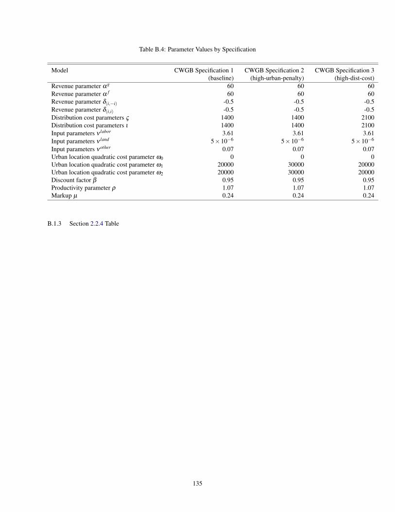
Table B.4: Parameter Values by Specification

Model CWGB Specification 1 CWGB Specification 2 CWGB Specification 3(baseline) (high-urban-penalty) (high-dist-cost)

Revenue parameter αg 60 60 60Revenue parameter α f 60 60 60Revenue parameter δ(i,−i) -0.5 -0.5 -0.5Revenue parameter δ(i,i) -0.5 -0.5 -0.5Distribution cost parameters ς 1400 1400 2100Distribution cost parameters ι 1400 1400 2100Input parameters ν labor 3.61 3.61 3.61Input parameters ν land 5×10−6 5×10−6 5×10−6

Input parameters νother 0.07 0.07 0.07Urban location quadratic cost parameter ω0 0 0 0Urban location quadratic cost parameter ω1 20000 30000 20000Urban location quadratic cost parameter ω2 20000 30000 20000Discount factor β 0.95 0.95 0.95Productivity parameter ρ 1.07 1.07 1.07Markup µ 0.24 0.24 0.24

B.1.3 Section 2.2.4 Table

135

Table B.5: Estimated Choice-Specific Value Function Models (OLS), Baseline Specification

Choice-Specifc Value Function Vi(agilt = 1) Vi(a

gilt = 0) Vi(a

filt = 1) Vi(a

filt = 0) Vi(ar

ilt = 1) Vi(arilt = 0) Vi(asc

ilt = 1) Vi(ascilt = 0)

Population 1.70×101*** 1.48×101*** 1.99×101*** 1.48×101*** 1.35×101*** 1.48×101*** 2.00×101*** 1.48×101***(1.15×100) (1.76×10−2) (8.53×10−1) (1.76×10−2) (5.99×10−1) (1.76×10−2) (5.99×10−1) (1.76×10−2)

Own Entry Regstore Allentown, PA -1.86×107 -1.38×107 -2.43×106 -7.22×106

(2.37×107) (1.26×107) (2.38×106) (6.51×106)Own Entry Regstore Boulder, CO -7.26×106 -6.26×106 -3.52×106

(1.91×107) (1.02×107) (5.26×106)Own Entry Regstore Hartford, CT -9.72×106 -6.68×106 -1.75×106 -3.73×106

(2.08×107) (1.08×107) (1.59×106) (5.56×106)Own Entry Regstore Kansas City, MO -1.33×107 -6.06×106 -1.89×106 -3.88×106

(2.37×107) (1.14×107) (2.11×106) (5.85×106)Own Entry Regstore San Francisco, CA NA NA NA

NA NA NAOwn Entry Regstore Augusta, GA -1.91×107 -3.10×106 -9.38×106

(1.51×107) (2.77×106) (7.76×106)Rival Entry Regstore Albany, GA NA NA NA NA

NA NA NA NARival Entry GM Dist Clarksville, TN -1.44×106*** -1.44×106*** -1.44×106*** -1.44×106***

(1.03×105) (1.03×105) (1.03×105) (1.03×105)Rival Entry GM Dist Columbia, MO -5.54×105*** -5.50×105*** -5.51×105*** -5.50×105***

(1.03×105) (1.03×105) (1.03×105) (1.03×105)Rival Entry GM Dist Cumberland, MD -2.35×106*** -2.35×106*** -2.35×106*** -2.35×106***

(1.03×105) (1.03×105) (1.03×105) (1.03×105)Rival Entry GM Dist Dover, DE -1.98×106*** -1.98×106*** -1.98×106*** -1.98×106***

(1.03×105) (1.03×105) (1.03×105) (1.03×105)Rival Entry GM Dist Hickory, NC -1.03×106*** -1.03×106*** -1.03×106*** -1.03×106***

(1.03×105) (1.03×105) (1.03×105) (1.03×105)Constant 2.77×107. 6.36×103 3.25×107** 5.08×103 2.27×106 4.31×103 1.48×107* 5.14×103

(1.58×107) (7.43×104) (1.18×107) (7.43×104) (2.22×106) (7.43×104) (6.04×106) (7.43×104)

Note: Each column represents an OLS regression model of the indicated choice-specific value function run only on the state variables selected by the corrresponding boosted regressionmodel f.

B.2 Section Details

B.2.1 Section 2.2.1 Details

Import Distribution Centers. During the 2000 to 2006 time period, Wal-Mart operated import distribution

centers in Mira Loma, CA, Statesboro, GA, Elwood, IL, Baytown, TX, and Williamsburg, VA.1 For our simulation

(over all time periods), we endow each firm with an import distribution center in each MSA in our sample physically

closest to the above listed cities. These include [with Wal-Mart’s corresponding import distribution center location in

brackets]: Riverside, CA [Mira Loma, CA], Savannah, GA [Statesboro, GA], Kankakee, IL [Elwood, IL], Houston,

TX [Baytown, TX], and Washington, DC [Williamsburg, VA].

General Merchandise and Food Distribution Centers. We constrain each competitor to open the same number

of general merchandise and food distribution centers in each period as actually opened by Wal-Mart. Additionally,

we constrain the competitor to open general merchandise and food distribution centers in the MSA’s in our sample

closest to the actual distribution centers opened by Wal-Mart in the same period. Tables B.1 and B.2 present both the

distribution centers opened by Wal-Mart, as well as the distribution center locations opened by the competitor in all

simulations.

B.2.2 Section 2.2.2 Details

State Space Cardinality Calculation. Calculations for the cardinality of the part of the state space attributable

to firm i as defined in our illustration are listed in Table B.3.

Constraints on firm location choices. For a given firm i, we allow each location l to accommodate up to

four firm i facilities at one time: one import distribution center, one food distribution center, one general merchandise

distribution center, and one store of either type. Symmetrically, the competitor firm can also place up to four facilities

in the same location l, for a maximum number of eight facilities per location. We assume that neither firm can place

two of its own stores (regardless of type) in one location. This approximates actual store placement patterns by big

box retailers such as Wal-Mart well for small MSA’s, which usually accommodate only one own-store at a time, but

less so for larger MSA’s, which might contain several own-stores. One additional constraint we impose is that in each

period t, each firm chooses regular stores prior to choosing supercenters. Since we allow only one firm i store of any

type per MSA, each firm’s constrained set of possible supercenter locations are a function of period t regular store

location choices.

Profit Specification. For a given firm i, sales revenues for a store in location l depend on the proximity of other

firm i stores and firm −i stores, where −i denotes the competitor firm. Note that since we allow only one store of any

1 See http://www.mwpvl.com/html/walmart.html for this list.

137

kind per MSA, we can refer to a store by its location, i.e. we refer to a store in location l as store l. Let the portion

of the state vector attributable to locations for food distribution centers ( f ), general merchandise distribution centers

(g), regular stores (r), and supercenters (sc) be denoted as s fit , sg

it ,srit , and ssc

it , where each vector is of length L, and

sqit ≡

(sq

1t , . . . ,sqLt

)for q ∈ { f ,g,r,sc}. Also denote the population for location l at time t as poplt . For store l of firm i

at time t, denote food revenues as R filt

(ssc

it ,ssc−it , poplt

)and general merchandise revenues as Rg

ilt (sit ,s−it , poplt), where

sit ≡ I(srit + ssc

it > 0) with support Sit , I(.) represents the indicator function, each element of sit is denoted as silt , food

revenues are a function of the proximity of supercenter locations for both firms, general merchandise revenues are a

function of the proximity of store locations of both types for both firms, and both classes of revenue are a function

location-specific population poplt .2 Although we do not model consumer choice explicitly, our revenue specification

implies that consumers view other own-stores and competitor-stores as substitutes for any given store.3

We assume that revenues are a function of the parameter vector ϑ i = (αi,δi,−i,δi,i) and specify total revenues for

store l and firm i at time t in the following way:

Rilt(ssc

it ,ssc−it ,sit ,s−it , poplt ;ϑ i

)= R f

ilt

(ssc

it ,ssc−it , poplt ;ϑ i

)+Rg

ilt (sit ,s−it , poplt ;ϑ i) (B.1)

where,

R filt

(ssc

it ,ssc−it , poplt ;ϑ i

)=

sscilt ∗

[αi poplt

(1+δi,−i ∑

m 6=l

ssc−imt

dlm∗ I{dlm ≤ 60}+δi,i ∑

m 6=l

sscimt

dlm∗ I{dlm ≤ 60}

)]

Rgilt (sit ,s−it , poplt ;ϑ i) =

silt ∗

[αi poplt

(1+δi,−i ∑

m 6=l

s−imt

dlm∗ I{dlm ≤ 60}+δi,i ∑

m 6=l

simt

dlm∗ I{dlm ≤ 60}

)]

In this specification, both classes of revenue depend on the proximity of own-stores and competitor-stores through

the terms δi,i ∑m6=l

syimt

dlm∗ I{dlm ≤ 60} and δi,−i ∑

m 6=l

sy−imtdlm∗ I{dlm ≤ 60} for y ∈ {sc,�}, respectively, where m indexes a

location different from location l, and dlm represents the distance from location l to a different location m. The

2 It is conceivable that close-proximity regular stores could cannibalize food revenues of a given supercenter store l to the extent that consumersbuy food incidentally while shopping for general merchandise. In that case, a nearby regular store might attract the business of these consumers,who could refrain from making the incidental food purchases they might have made at supercenter store l. Because we expect this effect to besmall, we model food revenues as conditional only on the presence of nearby supercenters.

3 Holmes (2011) specifies revenue in a similar way but derives consumers’ store substitution patterns from demand estimates obtained usingdata on Wal-Mart sales.

138

parameters δi,i and δi,−i represent the average effect on revenues of close-proximity own-stores and competitor-

stores, respectively. Since we assume that the parameters δi,i and δi,−i are negative, intuitively, these terms represent

a deduction to revenues induced by own-stores or competitor-stores that are close in proximity to store l, since

we assume that consumers view these stores as substitutes for store l. With respect to own-stores, this revenue

substitution effect is deemed own-store ”cannibalization,” which is an important dimension of chain-store location

decisions as documented by Holmes (2011) for the case of Wal-Mart. With respect to competitor stores, this effect

reflects competition. The strength of the effect is weighted by dlm, with stores in locations that are farther away from

store l having a smaller effect on revenues than those that are close by. The indicators I{dlm ≤ 60} take a value of

1 if location m is closer than 60 miles away from location l, 0 otherwise, which imposes the assumption that stores

located farther than 60 miles have no effect on store l revenues. This assumption is slightly unrealistic, but we impose

it since our sample only includes 227 MSA’s in the U.S., which means there are few MSA’s within, for example, a

30 mile radius of any MSA in our sample. With more MSA’s, this cutoff distance can be reduced. We assume that

the parameters δi,i and δi,−i are the same across revenue categories to simplify the exposition. Both types of revenue

are dependent on population at time t, xlt , through a common scalar parameter αi. Additionally, since regular stores

don’t sell food, R filt = 0 for all regular stores.

As in Holmes (2011), we abstract from price variation and assume each firm sets constant prices across all own-

stores and time, which is motivated by simplicity and is not necessarily far from reality for a chain-store retailer like

Wal-Mart, which is known to set prices according to an every-day-low-price strategy. Denoting µ as the proportion

of sales revenue that is net of the cost of goods sold (COGS), then µReilt (.) represents revenues net of COGS for firm

i, store l, time t, and revenue type e ∈ {g, f}.

Firms incur three types of additional costs: 1) distribution costs attributable to store sales, 2) store-level variable

costs, and store-level fixed costs. In order to sell a given set of goods in time period t at store l, as in Holmes

(2011), we assume that each firm incurs distribution costs to deliver these goods from general merchandise or food

distribution centers (or both for supercenters) to store l. In addition, we assume that firms incur distribution costs

when transporting these goods from import distribution centers to either general merchandise or food distribution

centers. We introduce these latter distribution costs in order to model location decisions for general merchandise and

food distribution centers. Denote the distribution costs incurred by firm i to sell goods from store l at time t as DCilt ,

which take the form: DCilt = ςdglt + ιdimp

lgt + ςd flt + ιdimp

l f t . Here, dglt and d f

lt represent the distance from store l to the

nearest firm i general merchandise distribution center or food distribution center, respectively. In our game simulation,

if store l is a regular store, we assume that it is supplied exclusively by the own-general merchandise distribution

center in the MSA physically closest to store l. Similarly, if store l is a supercenter, it is supplied exclusively by

the own-food distribution center and own-general merchandise distribution center in the MSA(’s) closest to store l.

Further, dimplgt represents the distance between the general merchandise distribution center that supplies store l and the

139

nearest import distribution center, while dimpl f t represents the distance between the food distribution center that supplies

store l (if store l is a supercenter) and the nearest import distribution center. We assume that distribution costs are

a fixed proportion of these distances, captured by the parameters ς and ι , and interpret fixed distribution costs as the

costs incurred to operate a truck over the course of one delivery of goods per day, aggregated over one year. This

model approximates the daily truck delivery distribution model actually employed by Wal-Mart, as documented by

Holmes (2011). Finally, if store l is a regular store, ςd flt + ιdimp

l f t = 0 since regular stores do not sell food.

The remainder of our costs for both firms are specified almost exactly as in Holmes (2011) for the case of Wal-

Mart, so we describe them succinctly and direct the interested reader to that work for additional description. Firms

incur variable costs in the form of labor, land, and other costs (all costs not attributable to land or labor). Variable

land costs are motivated by the store modification patterns of Wal-Mart, which frequently changes parking lot size,

building size, and shelf space to accommodate changes in sales patterns. The quantity of labor, land, and other

inputs needed are assumed to be a fixed proportion of total store revenues, such that for firm i, store l, and time t,

Laboreilt = νLaborRe

ilt , Landeilt = νLandRe

ilt , and Othereilt = νOtherRe

ilt , for merchandise segment e ∈ {g, f}. The prices

of land and labor per unit of input are represented by wages and rents specific to store l at time t, denoted as wagelt

and rentlt . We collect data on rents and wages for each time period and each MSA. We define rents as the median

(per-MSA) residential home value per square-foot from Zillow, and wages as the annual retail sector payroll divided

by the total number of employees (per-MSA), provided by the U.S. Census County Business Patterns dataset (MSA

level).4 The price of the other input is normalized to 1. We focus only on fixed costs that vary by location, since costs

that are constant across locations do not matter for the decision of where to locate stores and distribution centers. As

documented by Holmes (2011), there are disadvantages for big box retailers like Wal-Mart of locating stores in urban

locations, including, for example, increased non big box retailer shopping options for consumers. The fixed-cost

disadvantage of locating stores in urban locations is modeled as a as a function of the population density at time t of

the location hosting store l, denoted as Popdenlt .5 This function, u(Popdenlt), is quadratic in logs, e.g.:

u(Popdenlt) = ω0 +ω1 ln(Popdenlt)+ω2 ln(Popdenlt)2

Given this specification for revenues and costs, firm i operating profits for store l at time t take the following form:

πi (st)≈ πilt ≡[[

ψgilt − ςdg

lt − ιdimplgt

]+[ψ

filt − ςd f

lt − ιdimpl f t

]−u(Popdenlt)

](B.2)

where,4 The Zillow data is available from http://www.zillow.com/, and the Census data is available from http://www.census.gov/econ/cbp/.5 See Section 2.2.1 for details on our population density definition and data source.

140

ψeilt = µRe

ilt −WageltLaboreilt −RentltLande

ilt −Othereilt for merchandise segment e ∈ {g, f}

If store l is a regular store, the profit component[ψ

filt − ςd f

lt − ιdimpl f t

]= 0, since regular stores sell only general

merchandise. We assume that if firm i operates no store in location l at time t, then πilt = 0. Note that we use the ≈

notation to make clear that the we omit population density from the location-specific state described in Section 2.2.2

and instead only include location-specific population.

We define a discount factor β and set it to β = 0.95. As in Holmes (2011), we define an exogenous productivity

parameter ρ that represents gradual increases in average sales per-store, motivated by gradual increases in average

sales per-store experienced by Wal-Mart.6 Profit parameter values for each specification are presented in Table B.4.

B.2.3 Section 2.2.4 Details

Table B.5 presents OLS models of the choice-specific value functions of interest using state variables selected

by the corresponding boosted regression models in Table 2.1 and simulation data generated under the baseline speci-

fication of parameters.

6 Unlike in Holmes (2011), for simplicity of exposition, we make this productivity parameter constant over time. One source of these increasesis an expansion in the variety of products offered for sale.

141

Appendix C

Chapter 3 Appendix

Proof of Lemma 16. If E [D(1)Y (0)|X = x,T = 0] exists and if there are two known copula functions CL and

CU such that CL (u,v|x)≤C0 (u,v|x)≤CU (u,v|x) for all (u,v) ∈ [0,1]2, it follows from Mueller and Scarsini (2000),

Tchen (1980), and Tankov (2011) that

µL (x) =

∫ 1

0

∫ 1

0F−1

D(1)|T,X (u|0,X = x)F−1Y (0)|T,X (v|0,X = x)dCL (u,v|x) and

µU (x) =

∫ 1

0

∫ 1

0F−1

D(1)|T,X (u|0,X = x)F−1Y (0)|T,X (v|0,X = x)dCU (u,v|x) .

Assumptions 13 (i), 14, and 15 allow us to identify FY (0)|T,X (·|0,X = x) and FD(1)|T,X (·|0,X = x), since under As-

sumption 15, FD(1)|T,X (d|0,X = x) = FD(1)|T,X (d|1,X = x). The conclusion of the lemma follows from

F−1D(1)|T,X (u|0,X = x) =

0 if u ∈ [0,1− p(x)]

1 otherwise,

where p(x) is identified under Assumptions 13 (i) and 15, since

p(x) = Pr(D(1) = 1|X = x) = Pr(D(1) = 1|X = x,T = 1).

Proof of Theorem 19. From equation ( 3.1), we know that

θo(x) = AT T (x) = E[

T −λ

λ (1−λ )· D(1)− p(x)

p(x)(1− p(x))·Y |X = x

].

By the Law of Iterated Expectations (LIE), we obtain:

θo(x) = E[

E[

T −λ

λ (1−λ )· D(1)− p(x)

p(x)(1− p(x))·Y |X = x,T = t

]]= λ ·E

[1−λ

λ (1−λ )· D(1)− p(x)

p(x)(1− p(x))·Y (1) |X = x,T = 1

]+(1−λ ) ·E

[−λ

λ (1−λ )· D(1)− p(x)

p(x)(1− p(x))·Y (0) |X = x,T = 0

]= E

[D(1)− p(x)

p(x)(1− p(x))·Y (1) |X = x,T = 1

]−E

[D(1)− p(x)

p(x)(1− p(x))·Y (0) |X = x,T = 0

]. (C.1)

142

We note that, under Assumption 15, the propensity score p(x) is identified from sample information, since:

p(x) = λ ·Pr(D(1) = 1|X = x,T = 1)+(1−λ ) ·Pr(D(1) = 1|X = x,T = 0)

= λ ·Pr(D(1) = 1|X = x,T = 1)+(1−λ ) ·Pr(D(1) = 1|X = x,T = 1) (by Assump. 15)

= Pr(D(1) = 1|X = x,T = 1)

where Pr(D(1) = 1|X = x,T = 1) is identified from sample information. Therefore,

E[

D(1)− p(x)p(x)(1− p(x))

·Y (1) |X = x,T = 1]

in equation ( C.1) is identified from sample information. Further it is easy to see that

E[

D(1)− p(x)p(x)(1− p(x))

·Y (1) |X = x,T = 1]=

11− p(x)

(r1 (x,1)− r1 (x)) .

However, since D(1) is unobserved for the period T = 0 sample, without additional information, the expression

E[

D(1)−p(x)p(x)(1−p(x)) ·Y (0) |X = x,T = 0

]in equation ( C.1) is partially identified from sample information. To see this,

notice that:

E[

D(1)− p(x)p(x)(1− p(x))

·Y (0) |X = x,T = 0]

=1

p(x)(1− p(x))·E [D(1)Y (0) |X = x,T = 0]− 1

1− p(x)·E [Y (0) |X = x,T = 0] . (C.2)

In the right-hand-side expression, both E [Y (0) |X = x,T = 0] and p(x) are identified from sample information. But

µ (x) = E [D(1)Y (0) |X = x,T = 0] is not point-identified from sample information. However, Lemma 16 implies

that it is bounded: µL (x) ≤ µ (x) ≤ µU (x). Inserting these bounds into the right-hand-side of equation ( C.2) and

inserting equation ( C.2) into the right-hand-side of equation ( C.1) and rearranging provides θU (x) and θ L(x).

Proof of Theorem 20 . Notice that E[Y1 (1)−Y0 (1) |D(1) = 1] = EX |D(1)=1 [E[Y1 (1)−Y0 (1) |X = x,D(1) = 1]].

From the bounds in Theorem 19, under Assumptions (A1), (A2), (A3) (i) and (ii)’, and (A4), and assuming

E [D(1)Y (0)|X = x,T = 0] exists for each x ∈X , then E[Y1 (1)−Y0 (1) |X = x,D(1) = 1] = θo(x) is partially

identified for all x ∈X . The expectation EX |D(1)=1 [θ0(x)|D(1) = 1] is based on the distribution function Pr(X ≤

x|D(1) = 1) where:

Pr(X ≤ x|D(1) = 1) = λ ·Pr(X ≤ x|D(1) = 1,T = 1)+(1−λ ) ·Pr(X ≤ x|D(1) = 1,T = 0)

The distribution Pr(X ≤ x|D(1) = 1,T = 1) is identified from the period T = 1 sample, while λ is also identified from

143

sample information. Using Assumption 15, Pr(X ≤ x|D(1) = 1,T = 0) is identified from sample information, since:

Pr(X ≤ x|D(1) = 1,T = 0) =Pr(D(1) = 1,X ≤ x,T = 0)

Pr(D(1) = 1,T = 0)

=Pr(D(1) = 1,X ≤ x|T = 0)(1−λ )

Pr(D(1) = 1|T = 0)(1−λ )

=Pr(D(1) = 1|X ≤ x,T = 0)Pr(X ≤ x|T = 0)

Pr(D(1) = 1|T = 0)(C.3)

The denominator of the right-hand-side of equation C.3 can be expressed as:

Pr(D(1) = 1|T = 0) = Pr(D(1) = 1|X ≤ x,T = 0)Pr(X ≤ x|T = 0)

+Pr(D(1) = 1|X ≥ x,T = 0)Pr(X ≥ x|T = 0).

By Assumption 15, Pr(D(1) = 1|X ≥ x,T = 0) = Pr(D(1) = 1|X ≥ x,T = 1) and Pr(D(1) = 1|X ≤ x,T = 0) =

Pr(D(1) = 1|X ≤ x,T = 1), where both Pr(D(1) = 1|X ≥ x,T = 1) and Pr(D(1) = 1|X ≤ x,T = 1) are identified from

the period T = 1 sample. Finally, Pr(X ≤ x|T = 0) and Pr(X ≥ x|T = 0) are identified from the period T = 0 sample.

Proof of Theorem 23. Part (i): By the definition of X ≡ (W,Z), prior to utilizing the IV assumption, the bounds

in Theorem 19 can be written as:

θL(w,z) =

11− p(w,z)

[r1 (w,z,1)− r1 (w,z)+ r0 (w,z)−

µU (w,z)p(w,z)

]θ

U (w,z) =1

1− p(w,z)

[r1 (w,z,1)− r1 (w,z)+ r0 (w,z)−

µL (w,z)p(w,z)

]

where

µL (w,z) =

∫ 1

0

∫ 1

1−p(w,z)F−1

Y (0)|T,W,Z (v|0,W = w,Z = z)dCL (u,v|w,z) and

µU (w,z) =

∫ 1

0

∫ 1

1−p(w,z)F−1

Y (0)|T,W,Z (v|0,W = w,Z = z)dCU (u,v|w,z) .

By the LIE, ϕ01 (w,z) =

µ(w,z)p(w,z) . By Assumption 21 (i), ϕ0

1 (w,z) = ϕ01 (w). Therefore, the upper and lower bounds for

ϕ01 (w), denoted as ϕ0

1 (w)U and ϕ0

1 (w)L, respectively, are

ϕ01 (w)

L = supz

{µL (w,z)p(w,z)

}and ϕ

01 (w)

U = infz

{µU (w,z)p(w,z)

}.

The result θ LIV (w,z)≤ θo(w,z)≤ θU

IV (w,z) follows since µU (w,z) = p(w,z)ϕ01 (w)

U and µL (w,z) = p(w,z)ϕ01 (w)

L.

144

For the point identification result, notice that for any z ∈Z , by the LIE, we obtain:

E [Y (0)|W = w,Z = z] = p(w,z)ϕ01 (w,z)+(1− p(w,z))ϕ

00 (w,z) (C.4)

By Assumption 21 (i), ϕ0d (w,z) = ϕ0

d (w), so Equation C.4 becomes:

E [Y (0)|W = w,Z = z] = p(w,z)ϕ01 (w)+(1− p(w,z))ϕ

00 (w) (C.5)

which holds for all z ∈ Z. For z1,z2, . . . ,zm ∈Z , we obtain the system of equations formed by C.5:

Π

ϕ01 (w)

ϕ00 (w)

=

E[Y0(0)|W = w,Z = z1]

. . .

E[Y0(0)|W = w,Z = zm]

. (C.6)

By Assumptions 13 (i), 14, and 15, p(w,z) and E[Y0(0)|W = w,Z = z] are point-identified for all z ∈Z . So if Π has

rank 2, then

ϕ01 (w)

ϕ00 (w)

is point-identified. Under Assumption 22, Π has rank 2. Since θo(w,z) can be expressed

as

θo(w,z) =1

1− p(w,z)

[r1 (w,z,1)− r1 (w,z)+ r0 (w,z)−ϕ

01 (w)

](C.7)

this implies that θo(w,z) is point identified, since ϕ01 (w) is point identified and since under Assumptions 11, 12, 13

(i), 14, and 15, all other parameters in the expression for θo(w,z) are point-identified. We note that if m > 2, then

θo(w,z) may be over-identified.

Part (ii): The proof of this part begins exactly as under Part (i) in that, prior to utilizing the MIV assumption, the

bounds in Theorem 19 can be written as:

θL(w,z) =

11− p(w,z)

[r1 (w,z,1)− r1 (w,z)+ r0 (w,z)−

µU (w,z)p(w,z)

]θ

U (w,z) =1

1− p(w,z)

[r1 (w,z,1)− r1 (w,z)+ r0 (w,z)−

µL (w,z)p(w,z)

]

where

µL (w,z) =

∫ 1

0

∫ 1

1−p(w,z)F−1

Y (0)|T,W,Z (v|0,W = w,Z = z)dCL (u,v|w,z) and

µU (w,z) =

∫ 1

0

∫ 1

1−p(w,z)F−1

Y (0)|T,W,Z (v|0,W = w,Z = z)dCU (u,v|w,z) .

Again, by the LIE, ϕ01 (w,z) =

µ(w,z)p(w,z) . By Assumption 21 (ii) and given z1 ≤ z≤ z2, ϕ0

1 (w,z1)≤ ϕ01 (w,z)≤ ϕ0

1 (w,z2).

145

Therefore, the upper and lower bounds for ϕ01 (w,z), denoted as ϕ0

1 (w,z1)U and ϕ0

1 (w,z2)L, respectively, are

ϕ01 (w,z1)

L = supz1≤z

{µL (w,z1)

p(w,z1)

}and ϕ

01 (w,z2)

U = infz2≥z

{µU (w,z2)

p(w,z2)

}.

The result θ LMIV (w,z2)≤ θo(w,z)≤ θU

MIV (w,z1) follows since µU (w,z2) = p(w,z2)ϕ01 (w,z2)

U and

µL (w,z1) = p(w,z1)ϕ01 (w,z1)

L.

Part (iii): The expectation EW,Z|D(1)=1 [θo(W,Z)|D(1) = 1] is a function of θo(w,z) and Pr(W ≤ w,Z ≤ z|D(1) =

1). Part (i) establishes the sharp bounds for θo(w,z) for all z ∈ Z. By the LIE,

θo = E [Y (1)−Y (0)|D(1) = 1] = EW,Z|D(1)=1 [θo(W,Z)|D(1) = 1] .

As shown in the proof for Theorem 20, using Assumption 15, Pr(X ≤ x|D(1) = 1) is identified by sample infor-

mation. Since X ≡ (W,Z), Pr(W ≤ w,Z ≤ z|D(1) = 1) is identified from sample information. This, along with As-

sumptions 11, 12, 13 (i), 14, 15, and 21 (i), establish θ LIV ≤ θo ≤ θU

IV . Under Assumption 22, Π has rank 2 and θo(w,z)

is point-identified for each z ∈Z . θo is point-identified since by the LIE, θo = EW,Z|D(1)=1 [θo(W,Z)|D(1) = 1].

Proof of Theorem 32. Under Assumptions 11 and 12, it is well-known that θo(x) is point-identified by:

θo(x) = r1 (x,1)− r0 (x,1)−{r1 (x,0)− r0 (x,0)}

See Heckman et al. (1997). Under Assumptions 26 (i) and (ii), r1 (x,1,1), r0 (x,1,1), r1 (x,0,1), and r0 (x,0,1) are

point-identified. Under Assumption 30, we have that:

r1 (x,1)− r0 (x,1)−{r1 (x,0)− r0 (x,0)}= r1 (x,1,1)− r0 (x,1,1)−{r1 (x,0,1)− r0 (x,0,1)}

which implies that θo(x) is point-identified. If Assumption 11 holds for all x ∈X , then θo(x) is point-identified for

each x ∈X . By the LIE,

θo = EX |D(1)=1 [θo(x)|D(1) = 1] (C.8)

where the expectation in C.8 is based on the distribution function Pr(X ≤ x|D(1) = 1). Assumptions 26 (i) and

(ii) point-identify Pr(X ≤ x|D(1) = 1,M = 1) for all x ∈X , which in turn point-identifies Pr(X ≤ x|D(1) = 1) for

all x ∈X using Assumption 31. The result follows.

Proof of Theorem 34. Part (i): By the LIE,

θo(x) = Pr(M = 1|X = x)θo(x,1)+Pr(M = 0|X = x)θo(x,0). (C.9)

146

Under Assumption 29, Pr(M = 1|X = x) is known. Under Assumptions 24, 25, 26 (i) and (ii), θo(x,1) is also

point-identified, since

θo(x,1) = r1 (x,1,1)− r0 (x,1,1)−{r1 (x,0,1)− r0 (x,0,1)} .

Now consider θo(x,0). Under 24 and 25, this parameter can be re-expressed as

θo(x,0) =1

1− p(x,0)

[r1 (x,1,0)− r1 (x,0)+ r0 (x,0)−

E [D(1)Y (0)|X = x,T = 0,M = 0]p(x,0)

](C.10)

By Assumption 28 and the LIE, p(x,0) is point-identified by Pr(D(1) = 1|T = 1,X = x,M = 0). Also, under

Assumptions 26 (i) and 27, the expectations r1 (x,1,0), r1 (x,0), and r0 (x,0) are identified by sample information.

However, since for the unmatched (M = 0) sample, Y (0) and D(1) are not jointly observed in the period T = 0 sample,

E [D(1)Y (0)|X = x,T = 0,M = 0] is not necessarily point-identified. Let µ(x)M=0 =E [D(1)Y (0)|X = x,T = 0,M = 0].

Since by assumption E [D(1)Y (0)|X = x,T = 0,M = 0] exists and there are two known copula functions CL and CU

such that CL (u,v|x,M = 0) ≤ C0 (u,v|x,M = 0) ≤ CU (u,v|x,M = 0) for all (u,v) ∈ [0,1]2, it follows from Mueller

and Scarsini (2000), Tchen (1980), and Tankov (2011), that

µL(x)M=0 =

∫ 1

0

∫ 1

1−p(x,0)F−1

Y (0)|T,X ,M (v|0,X = x,0)dCL (u,v|x,M = 0) (C.11)

µU (x)M=0 =

∫ 1

0

∫ 1

1−p(x,0)F−1

Y (0)|T,X ,M (v|0,X = x,0)dCU (u,v|x,M = 0)

since F−1D(1)|T,X ,M (u|0,X = x,0) =

0 if u ∈ [0,1− p(x,0)]

1 otherwise.

Under Assumption 27, FY (0)|T,X ,M (·|0,X = x,0) is identified by sample information. It follows that θo(x,0) is

partially identified by θ L(x,0)≤ θo(x,0)≤ θU (x,0), where

θL(x,0) =

11− p(x,0)

[r1 (x,1,0)− r1 (x,0)+ r0 (x,0)−

µU (x)M=0

p(x,0)

]and

θU (x,0) =

11− p(x,0)

[r1 (x,1,0)− r1 (x,0)+ r0 (x,0)−

µL(x)M=0

p(x,0)

].

Substituting these bounds into equation C.9 gives

θLM(x) = Pr(M = 1|X = x)θo(x,1)+Pr(M = 0|X = x)θ L(x,0) and

θUM(x) = Pr(M = 1|X = x)θo(x,1)+Pr(M = 0|X = x)θU (x,0).

Without further restrictions, there bounds are sharp.

147

Part (ii): Deriving the sharp bounds for θo is straightforward. By the LIE, θo =EX |D(1)=1 [θo(X)|D(1) = 1]. Since

E [D(1)Y (0)|X = x,T = 0,M = 0] exists for each x ∈X , by Assumptions 24, 25, 26 (i) and (ii), 27, 28, 29, and 33,

θo(x) is partially identified by θ LM(x)≤ θo(x)≤ θU

M(x) as above for each x ∈X . EX |D(1)=1 [θ0(X)|D(1) = 1] exists

and is based on the distribution function

Pr(X ≤ x|D(1) = 1) = Pr(M = 1|D(1) = 1)Pr(X ≤ x|D(1) = 1,M = 1)

+Pr(M = 0|D(1) = 1)Pr(X ≤ x|D(1) = 1,M = 0)

By Assumptions 26 (i) and (ii), Pr(M = 1|D(1) = 1) and Pr(X ≤ x|D(1) = 1,M = 1) are identified by sample infor-

mation. By Assumptions 28, 26 (i) and (ii), Pr(X ≤ x|D(1) = 1,M = 0) is identified by sample information. The

probability Pr(M = 0|D(1) = 1) is identified from sample information, since

Pr(M = 0|D(1) = 1) =Pr(M = 0,D(1) = 1)

Pr(D(1) = 1)

=Pr(D(1) = 1|M = 0)Pr(M = 0)

Pr(D(1) = 1)

and each component Pr(D(1) = 1|M = 0), Pr(M = 0), and Pr(D(1) = 1) is identified by sample information under

Assumptions 28, 26 (i), 27, and 29. Since Assumption 24 holds for all x ∈X , the result follows.

148