Atmospheric Water and Precipitation

• Global energy balance• Atmospheric circulation• Atmospheric water vapor• Precipitation

• Reading: Sections 3.1 to 3.4

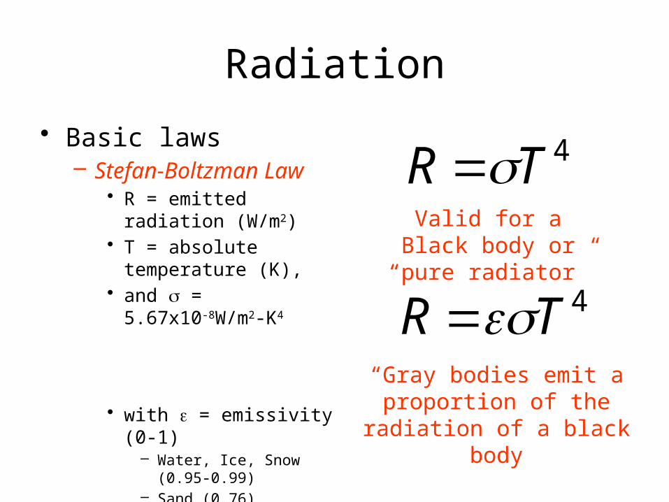
Radiation

• Basic laws– Stefan-Boltzman Law

• R = emitted radiation (W/m2)

• T = absolute temperature (K),

• and s = 5.67x10-8W/m2-K4

• with e = emissivity (0-1)– Water, Ice, Snow (0.95-0.99)– Sand (0.76)

4TR

“Gray bodies emit a proportion of the radiation

of a black body

4TR

Valid for a Black body or “pure radiator”

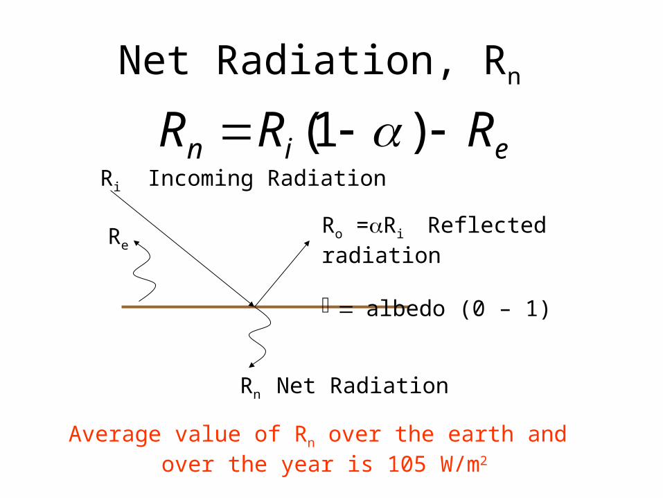
Net Radiation, Rn

Ri Incoming Radiation

Ro =aRi Reflected radiation

a= albedo (0 – 1)

Rn Net Radiation

Re

ein RRR )1(

Average value of Rn over the earth and over the year is 105 W/m2

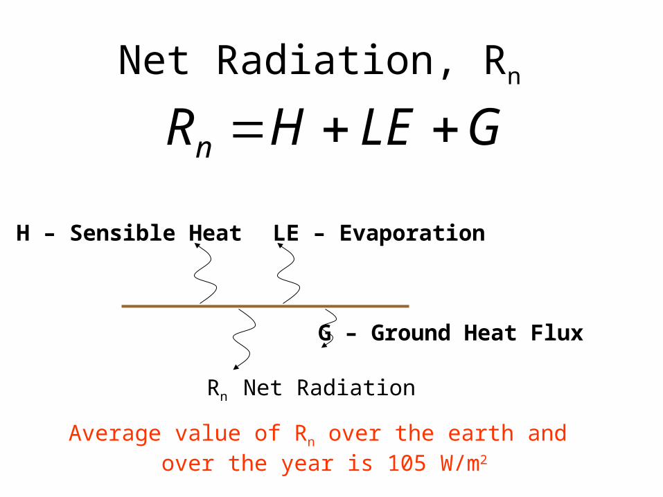
Net Radiation, Rn

Rn Net Radiation

GLEHRn

Average value of Rn over the earth and over the year is 105 W/m2

G – Ground Heat Flux

LE – EvaporationH – Sensible Heat

http://www.uwsp.edu/geo/faculty/ritter/geog101/textbook/energy/radiation_balance.html

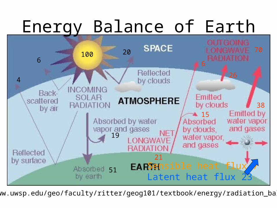
Energy Balance of Earth

6

4

10070

51

21

26

38

6

20

15

Sensible heat flux 7Latent heat flux 23

19

-600

-400

-200

0

200

400

600

D_Sho

rt

U_Sho

rt

D_Lon

g

U_Lon

g

Groun

d

Late

nt

Sensib

le Flu

x (

W/m

2)

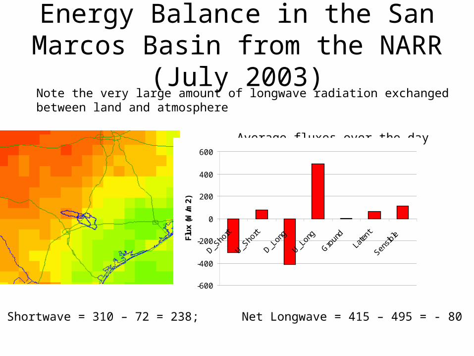
Energy Balance in the San Marcos Basin from the NARR (July 2003)

Average fluxes over the day

310

72

415

495

361

112

Net Shortwave = 310 – 72 = 238; Net Longwave = 415 – 495 = - 80

Note the very large amount of longwave radiation exchanged between land and atmosphere

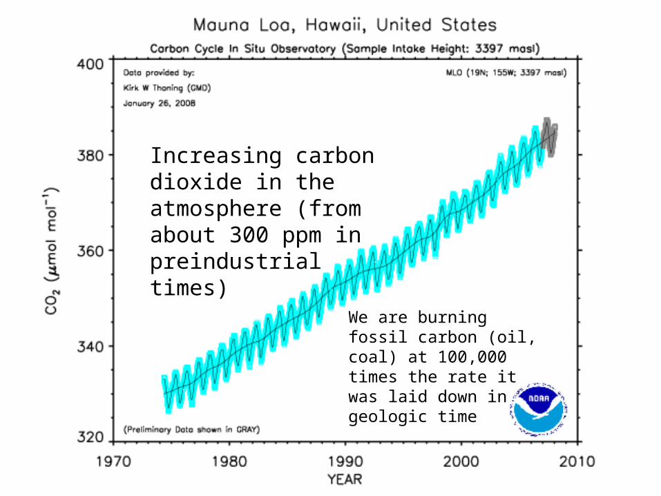
Increasing carbon dioxide in the atmosphere (from about 300 ppm in preindustrial times)

We are burning fossil carbon (oil, coal) at 100,000 times the rate itwas laid down in geologic time

Absorption of energy by CO2

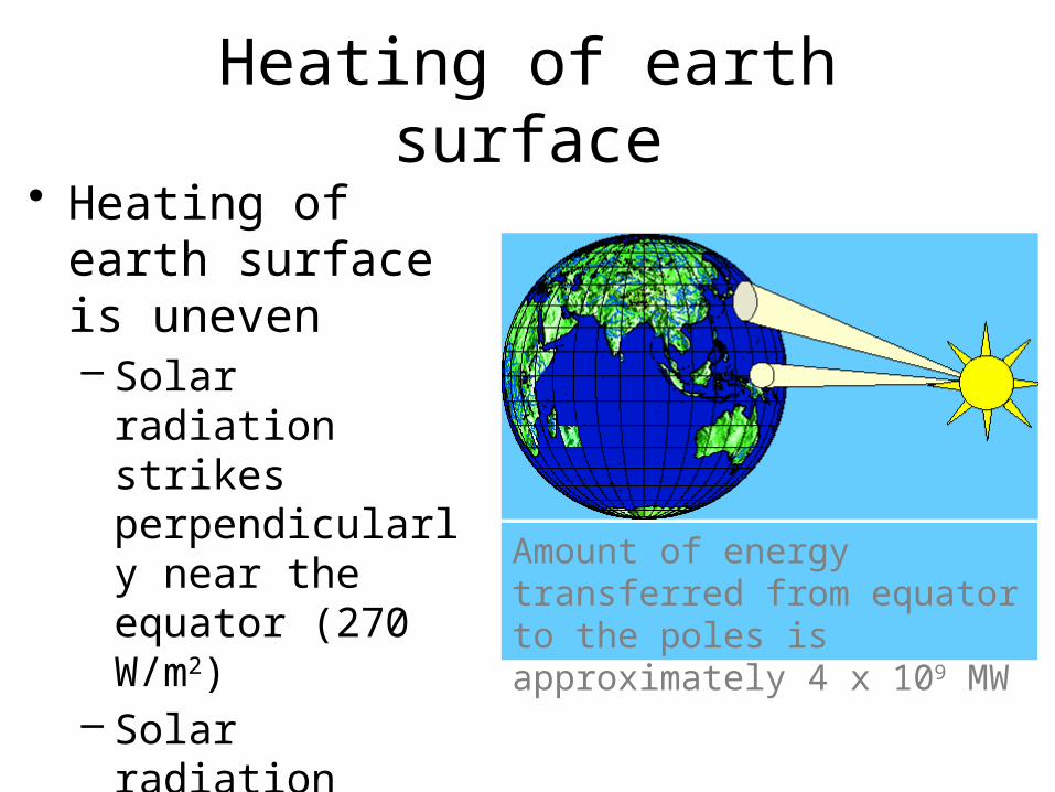
Heating of earth surface• Heating of earth

surface is uneven– Solar radiation

strikes perpendicularly near the equator (270 W/m2)

– Solar radiation strikes at an oblique angle near the poles (90 W/m2)

• Emitted radiation is more uniform than incoming radiation

Amount of energy transferred from equator to the poles is approximately 4 x 109 MW

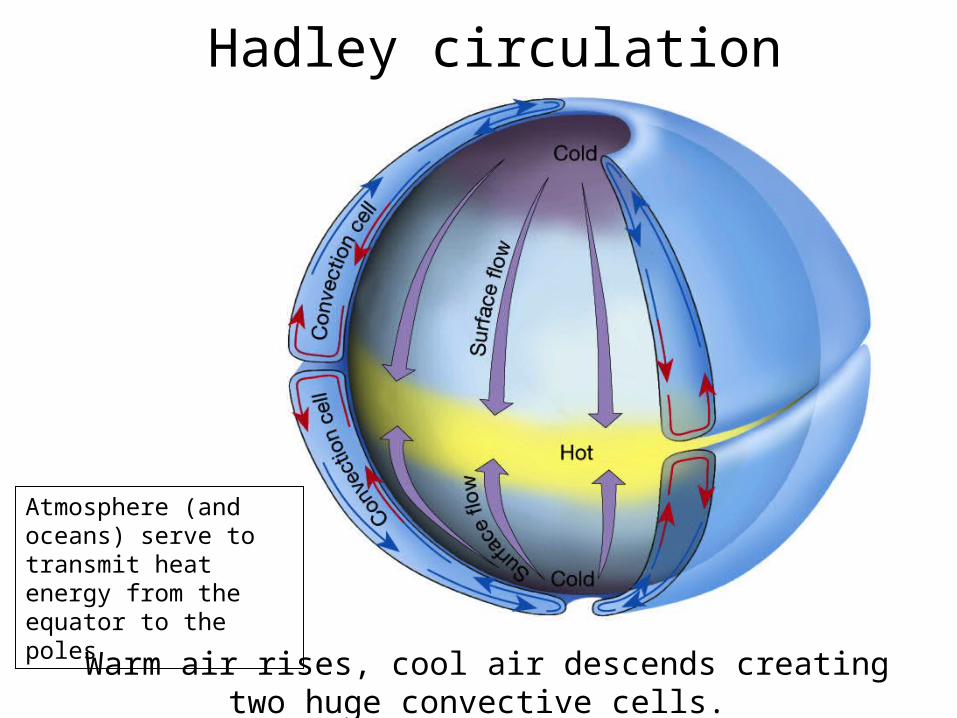
Hadley circulation

Warm air rises, cool air descends creating two huge convective cells.

Atmosphere (and oceans) serve to transmit heat energy from the equator to the poles

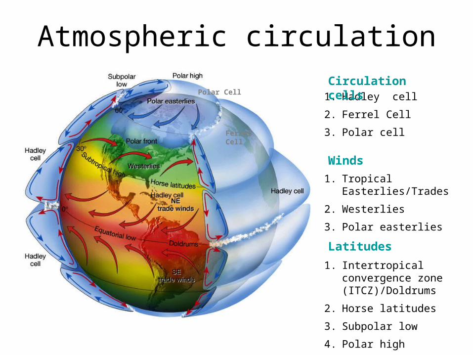
Atmospheric circulation

1. Tropical Easterlies/Trades

2. Westerlies

3. Polar easterlies

1. Intertropical convergence zone (ITCZ)/Doldrums

2. Horse latitudes

3. Subpolar low

4. Polar high

Ferrel Cell

Polar Cell 1. Hadley cell

2. Ferrel Cell

3. Polar cell

Latitudes

Winds

Circulation cells

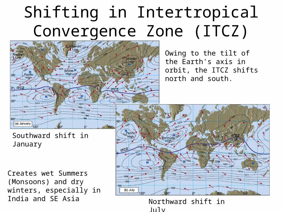
Shifting in Intertropical Convergence Zone (ITCZ)

Owing to the tilt of the Earth's axis in orbit, the ITCZ shifts north and south. 

Southward shift in January

Northward shift in July

Creates wet Summers (Monsoons) and dry winters, especially in India and SE Asia

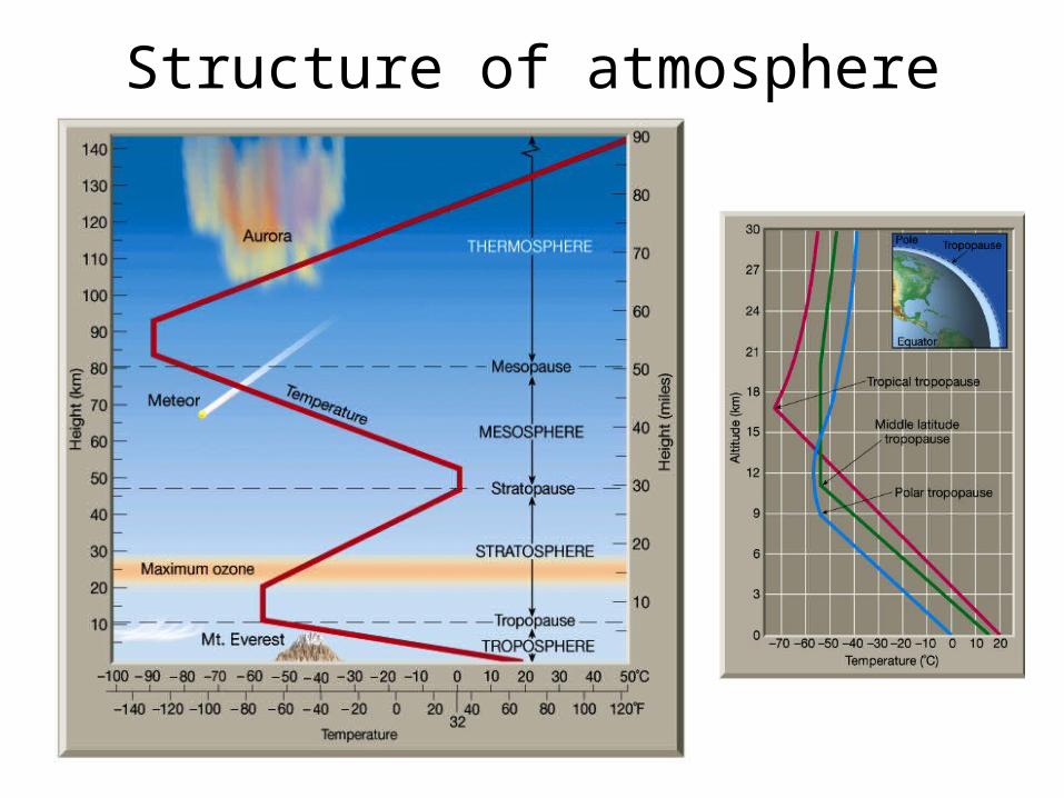
Structure of atmosphere

Atmospheric water

• Atmospheric water exists – Mostly as gas or water vapor– Liquid in rainfall and water droplets in clouds– Solid in snowfall and in hail storms

• Accounts for less than 1/100,000 part of total water, but plays a major role in the hydrologic cycle

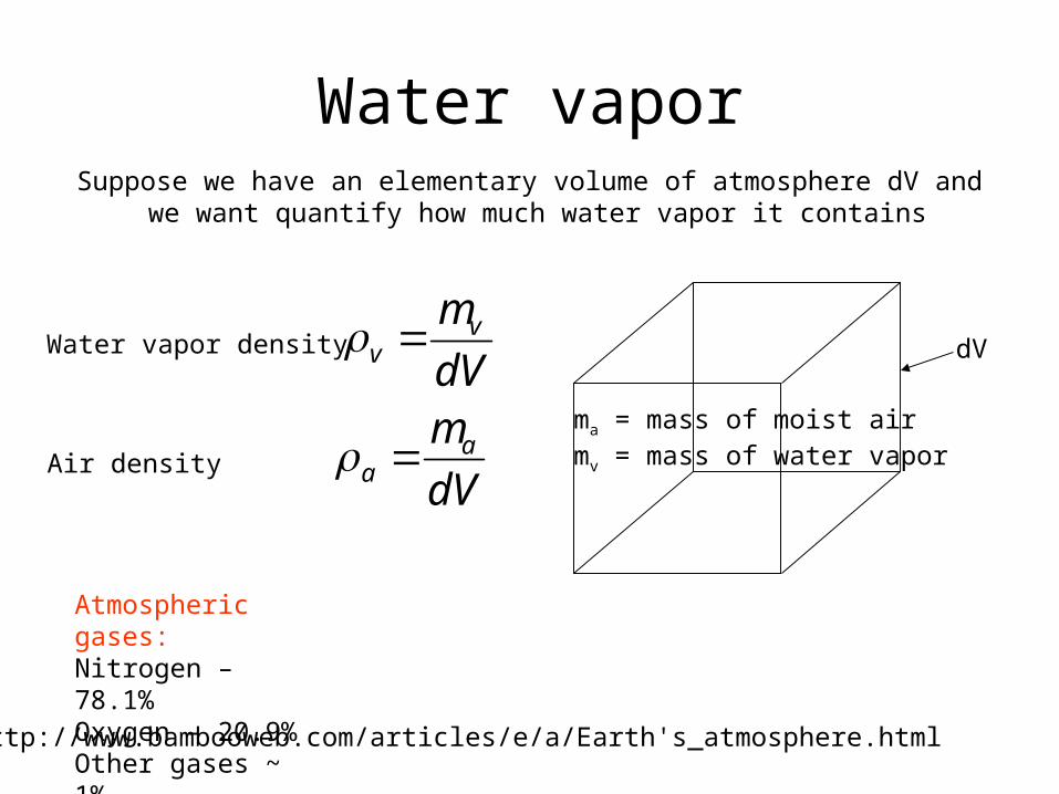
Water vaporSuppose we have an elementary volume of atmosphere dV and

we want quantify how much water vapor it contains

Atmospheric gases:Nitrogen – 78.1%Oxygen – 20.9%Other gases ~ 1%

http://www.bambooweb.com/articles/e/a/Earth's_atmosphere.html

dV

ma = mass of moist airmv = mass of water vapor

dV

mvv Water vapor density

dV

maa Air density

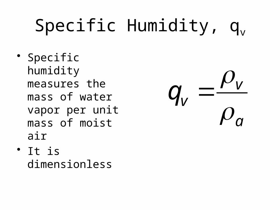
Specific Humidity, qv

• Specific humidity measures the mass of water vapor per unit mass of moist air

• It is dimensionlessa

vvq

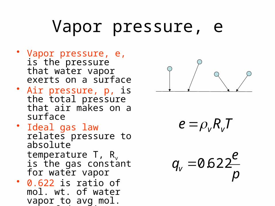
Vapor pressure, e• Vapor pressure, e, is the

pressure that water vapor exerts on a surface

• Air pressure, p, is the total pressure that air makes on a surface

• Ideal gas law relates pressure to absolute temperature T, Rv is the gas constant for water vapor

• 0.622 is ratio of mol. wt. of water vapor to avg mol. wt. of dry air (=18/28.9)

TRe vv

p

eqv 622.0

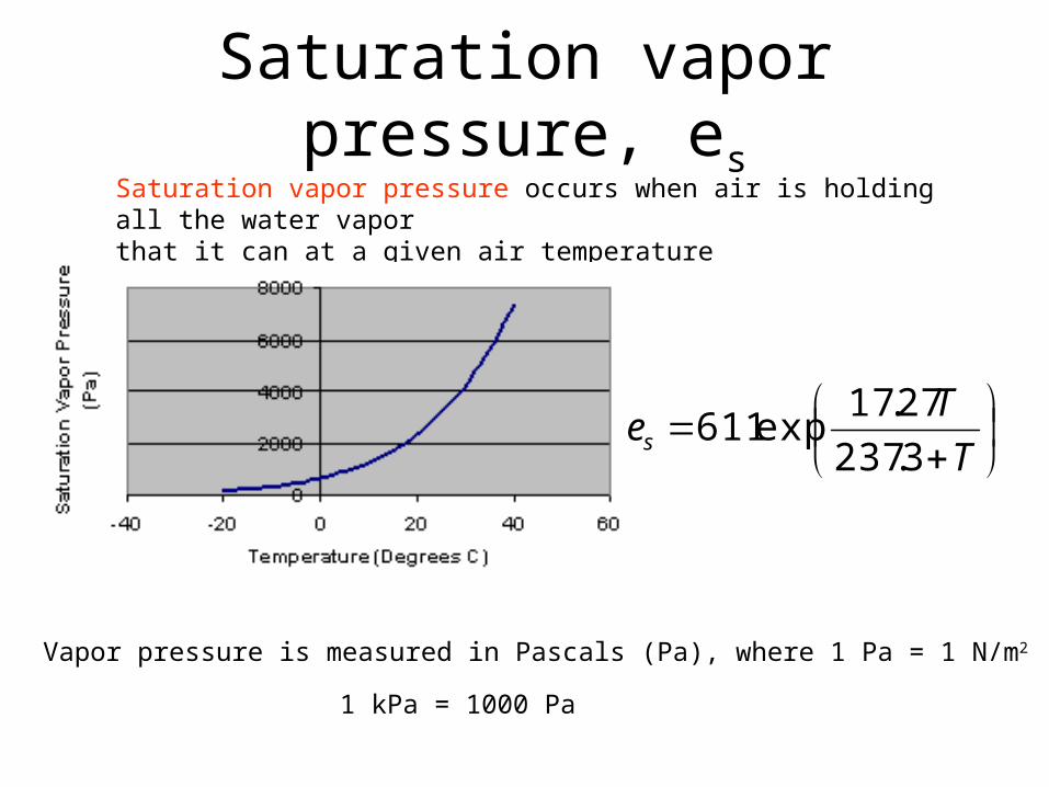
Saturation vapor pressure, es

Saturation vapor pressure occurs when air is holding all the water vaporthat it can at a given air temperature

T

Tes 3.237

27.17exp611

Vapor pressure is measured in Pascals (Pa), where 1 Pa = 1 N/m2

1 kPa = 1000 Pa

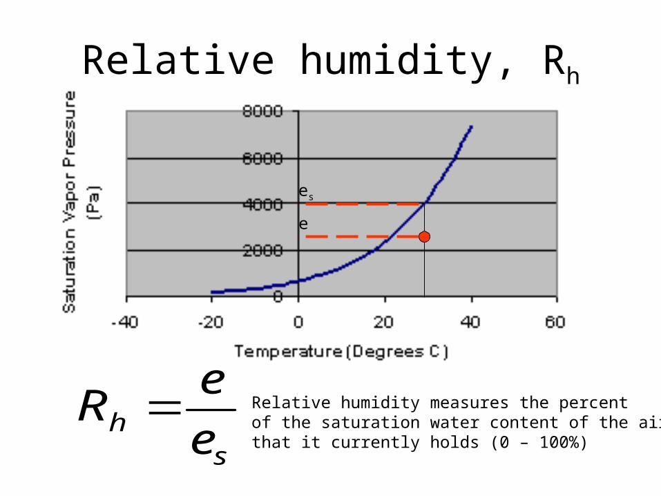
Relative humidity, Rh

es

e

sh e

eR Relative humidity measures the percent

of the saturation water content of the airthat it currently holds (0 – 100%)

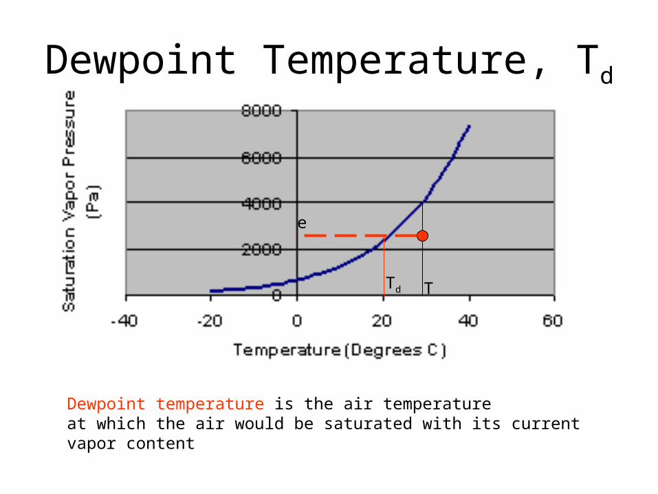
Dewpoint Temperature, Td

e

Dewpoint temperature is the air temperatureat which the air would be saturated with its current vapor content

TTd

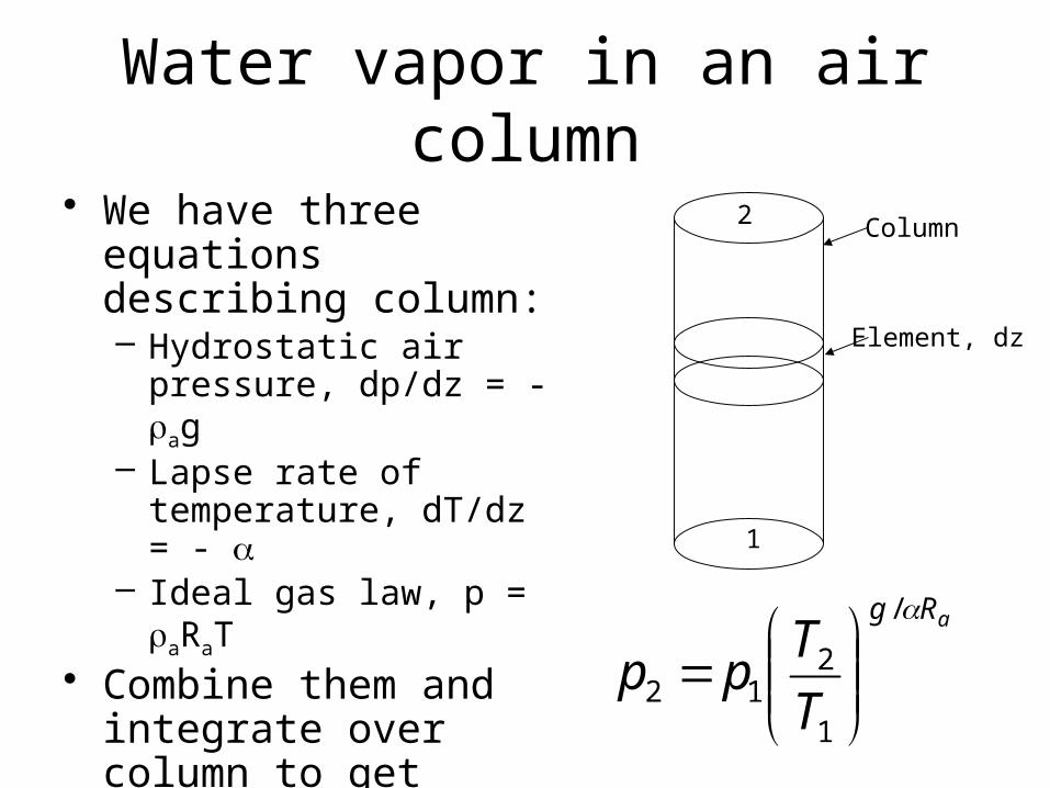
Water vapor in an air column

• We have three equations describing column:– Hydrostatic air pressure,

dp/dz = -rag– Lapse rate of temperature,

dT/dz = - a– Ideal gas law, p = raRaT

• Combine them and integrate over column to get pressure variation elevation

Column

Element, dz

aRg

T

Tpp

/

1

212

1

2

Precipitable Water

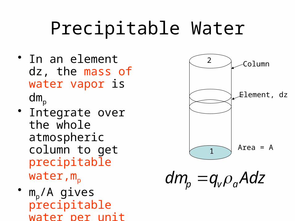
• In an element dz, the mass of water vapor is dmp

• Integrate over the whole atmospheric column to get precipitable water,mp

• mp/A gives precipitable water per unit area in kg/m2

Column

Element, dz

1

2

Adzqdm avp

Area = A

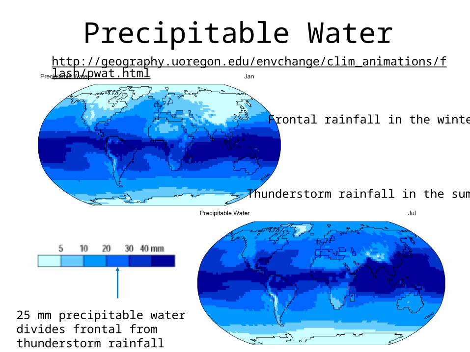
Precipitable Waterhttp://geography.uoregon.edu/envchange/clim_animations/flash/pwat.html

25 mm precipitable water divides frontal from thunderstorm rainfall

Frontal rainfall in the winter

Thunderstorm rainfall in the summer

Precipitation

• Precipitation: water falling from the atmosphere to the earth.– Rainfall– Snowfall– Hail, sleet

• Requires lifting of air mass so that it cools and condenses.

Mechanisms for air lifting

1. Frontal lifting

2. Orographic lifting

3. Convective lifting

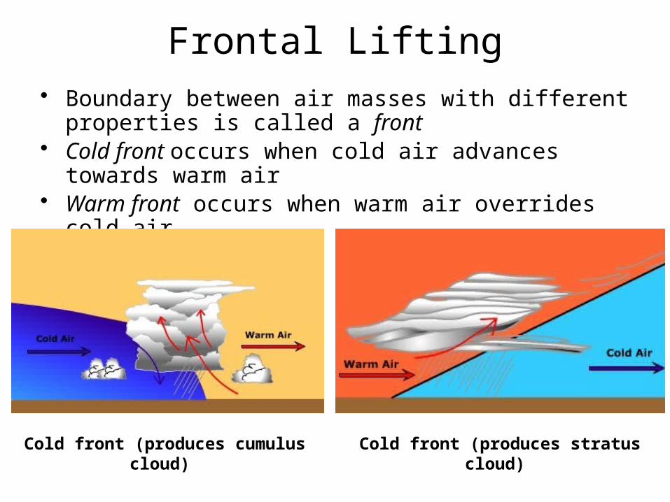
Frontal Lifting• Boundary between air masses with different properties is

called a front• Cold front occurs when cold air advances towards warm

air• Warm front occurs when warm air overrides cold air

Cold front (produces cumulus cloud)

Cold front (produces stratus cloud)

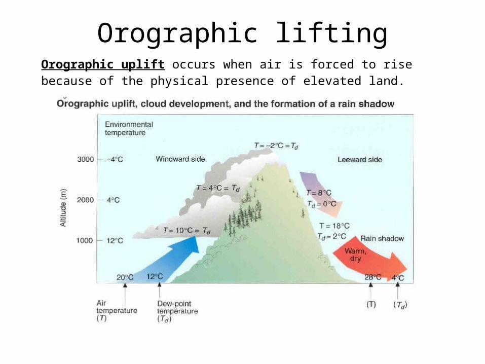
Orographic liftingOrographic uplift occurs when air is forced to rise because of the physical presence of elevated land.

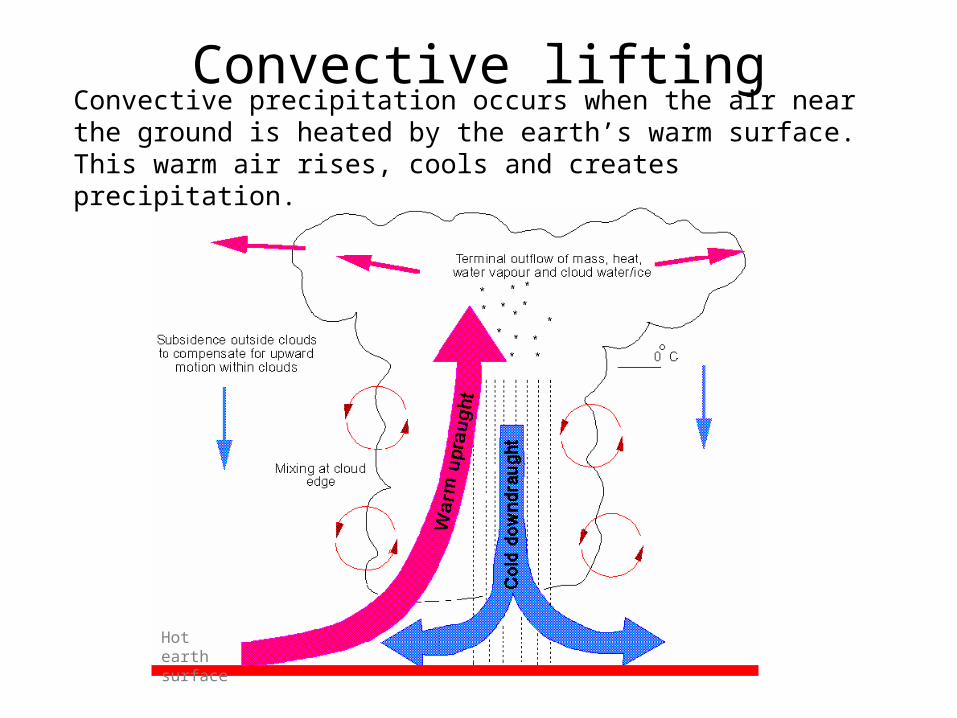
Convective lifting

Hot earth surface

Convective precipitation occurs when the air near the ground is heated by the earth’s warm surface. This warm air rises, cools and creates precipitation.

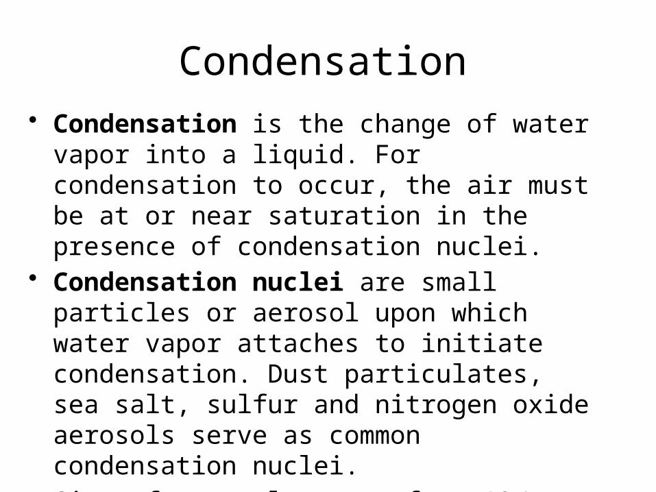
Condensation• Condensation is the change of water vapor into

a liquid. For condensation to occur, the air must be at or near saturation in the presence of condensation nuclei.

• Condensation nuclei are small particles or aerosol upon which water vapor attaches to initiate condensation. Dust particulates, sea salt, sulfur and nitrogen oxide aerosols serve as common condensation nuclei.

• Size of aerosols range from 10-3 to 10 mm.

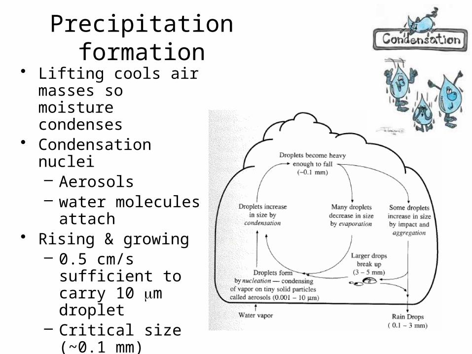
Precipitation formation• Lifting cools air masses

so moisture condenses• Condensation nuclei

– Aerosols – water molecules

attach• Rising & growing

– 0.5 cm/s sufficient to carry 10 mm droplet

– Critical size (~0.1 mm)

– Gravity overcomes and drop falls

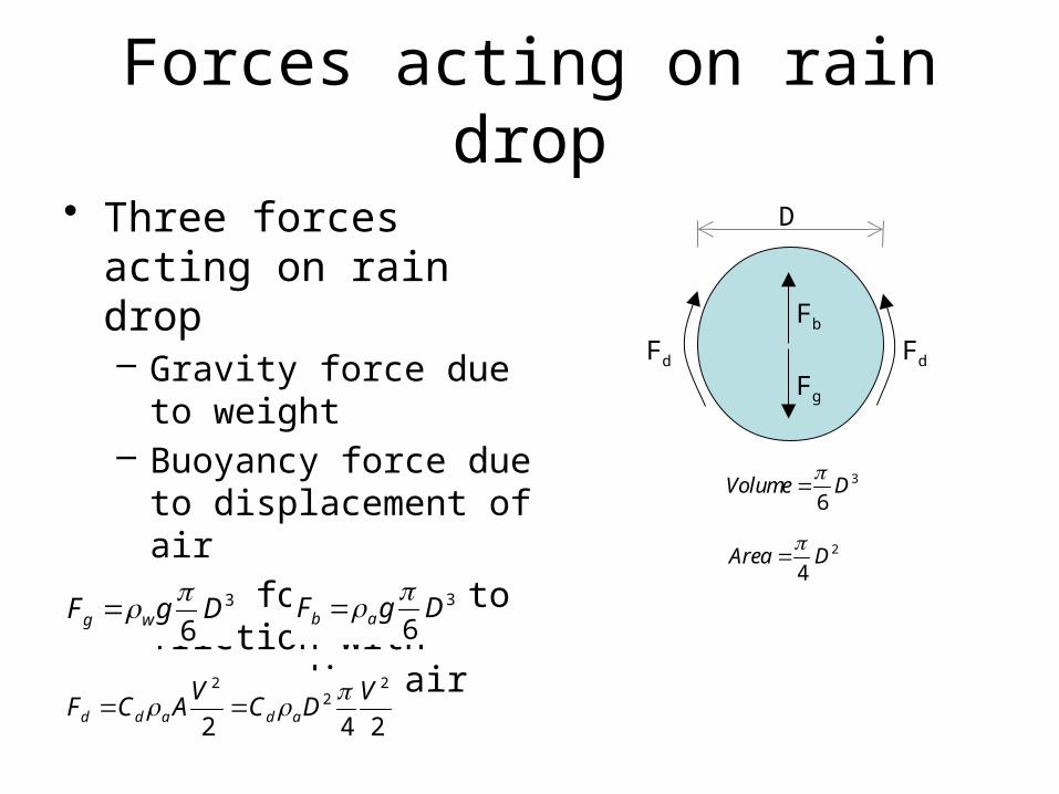
Forces acting on rain drop

FdFd

Fb

Fg

D• Three forces acting on rain drop– Gravity force due to

weight– Buoyancy force due to

displacement of air– Drag force due to friction

with surrounding air

3

6DVolume

2

4DArea

3

6DgF wg

3

6DgF ab

242

22

2 VDC

VACF adadd

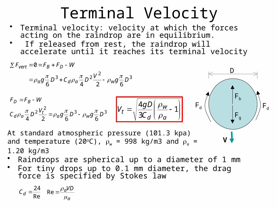
Terminal Velocity• Terminal velocity: velocity at which the forces acting on the raindrop

are in equilibrium.• If released from rest, the raindrop will accelerate until it reaches its

terminal velocity

32

23

6246

0

DgV

DCDg

WFFF

wada

DBvert

332

2

6624DgDg

VDC

WFF

wat

ad

BD

1

3

4

a

w

dt C

gDV

• Raindrops are spherical up to a diameter of 1 mm• For tiny drops up to 0.1 mm diameter, the drag force is specified by

Stokes law

FdFd

Fb

Fg

D

V

Re

24dCa

aVD

Re

At standard atmospheric pressure (101.3 kpa) and temperature (20oC), rw = 998 kg/m3 and ra = 1.20 kg/m3

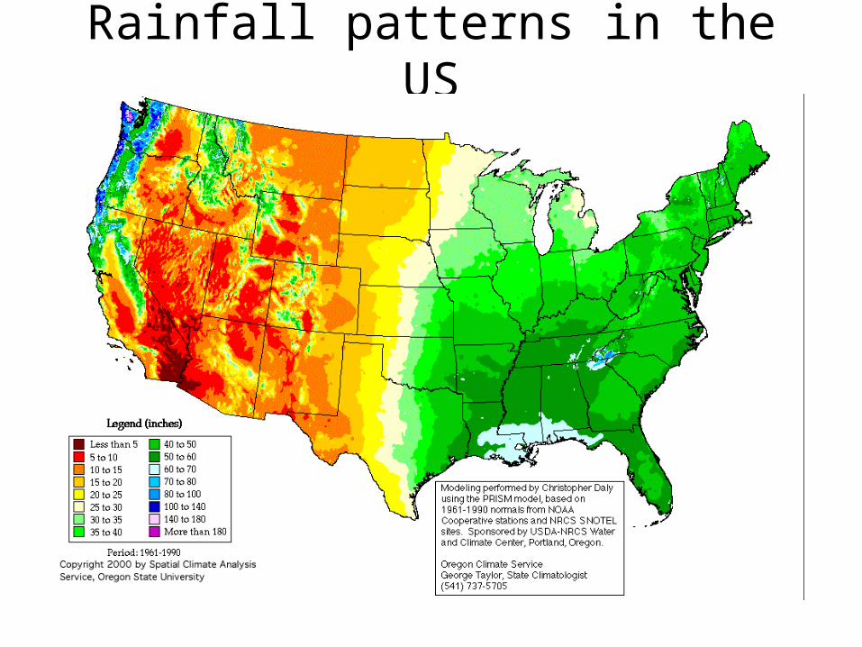
Rainfall patterns in the US

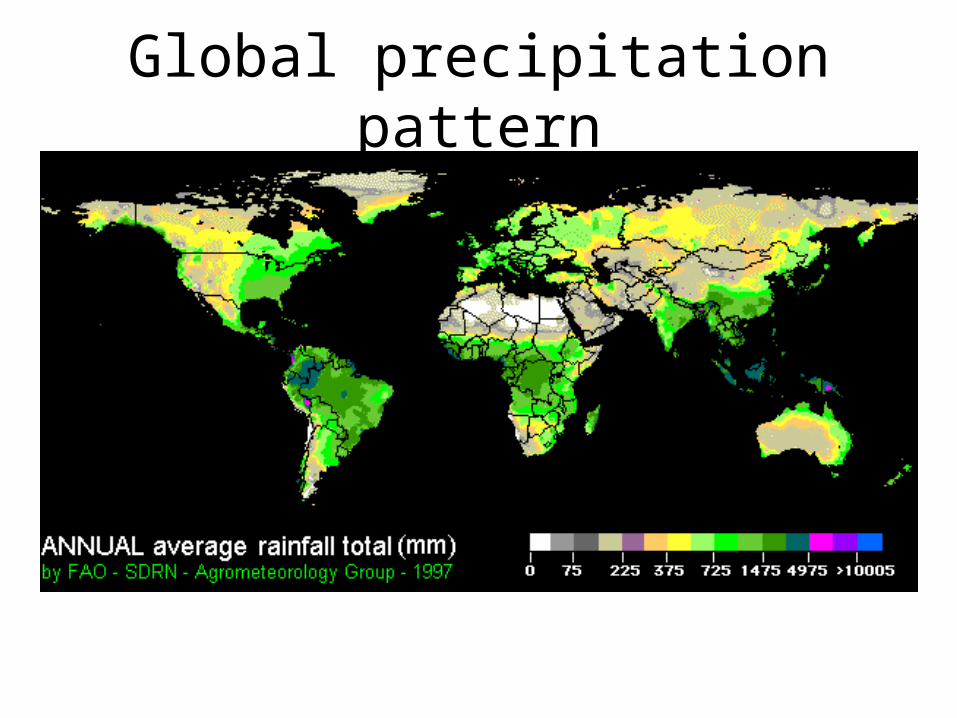
Global precipitation pattern

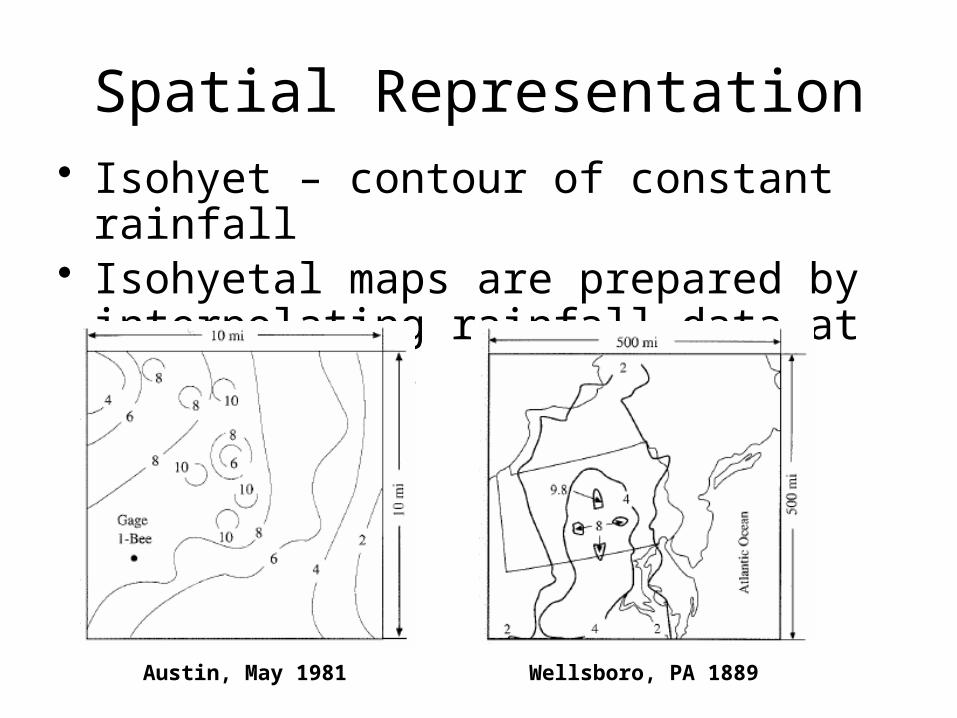
Spatial Representation• Isohyet – contour of constant rainfall• Isohyetal maps are prepared by

interpolating rainfall data at gaged points.

Austin, May 1981 Wellsboro, PA 1889

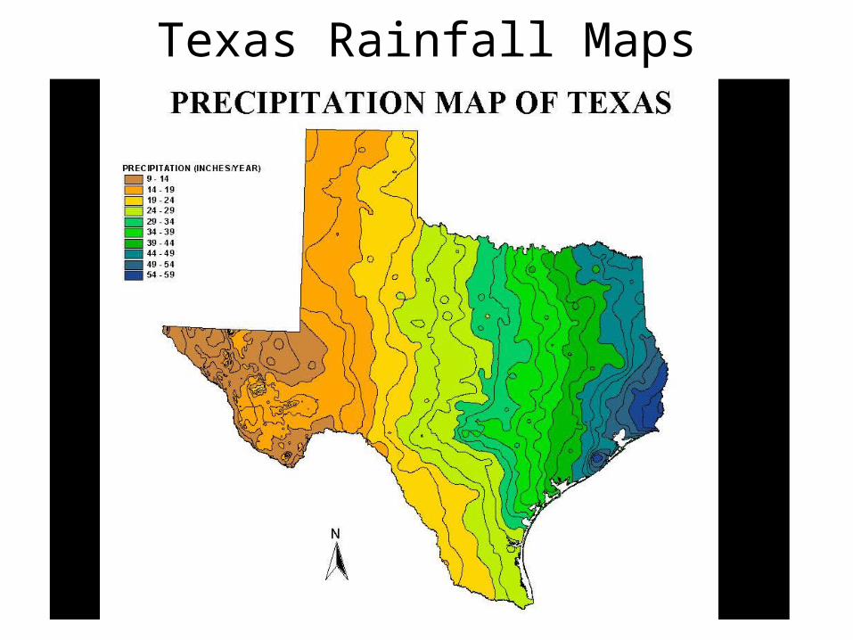
Texas Rainfall Maps

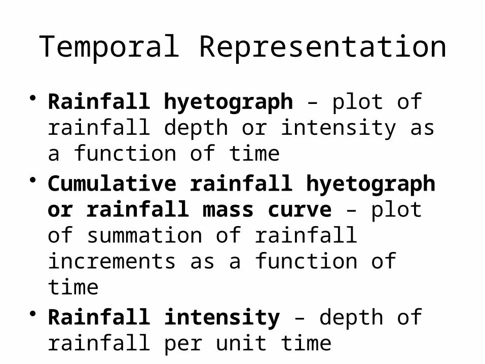
Temporal Representation

• Rainfall hyetograph – plot of rainfall depth or intensity as a function of time

• Cumulative rainfall hyetograph or rainfall mass curve – plot of summation of rainfall increments as a function of time

• Rainfall intensity – depth of rainfall per unit time

Rainfall Depth and IntensityTime (min) Rainfall (in) Cumulative 30 min 1 h 2 h

Rainfall (in)0 05 0.02 0.0210 0.34 0.3615 0.1 0.4620 0.04 0.525 0.19 0.6930 0.48 1.17 1.1735 0.5 1.67 1.6540 0.5 2.17 1.8145 0.51 2.68 2.2250 0.16 2.84 2.3455 0.31 3.15 2.4660 0.66 3.81 2.64 3.8165 0.36 4.17 2.5 4.1570 0.39 4.56 2.39 4.275 0.36 4.92 2.24 4.4680 0.54 5.46 2.62 4.9685 0.76 6.22 3.07 5.5390 0.51 6.73 2.92 5.5695 0.44 7.17 3 5.5100 0.25 7.42 2.86 5.25105 0.25 7.67 2.75 4.99110 0.22 7.89 2.43 5.05115 0.15 8.04 1.82 4.89120 0.09 8.13 1.4 4.32 8.13125 0.09 8.22 1.05 4.05 8.2130 0.12 8.34 0.92 3.78 7.98135 0.03 8.37 0.7 3.45 7.91140 0.01 8.38 0.49 2.92 7.88145 0.02 8.4 0.36 2.18 7.71150 0.01 8.41 0.28 1.68 7.24Max. Depth 0.76 3.07 5.56 8.2Max. Intensity 9.12364946 6.14 5.56 4.1

Running Totals

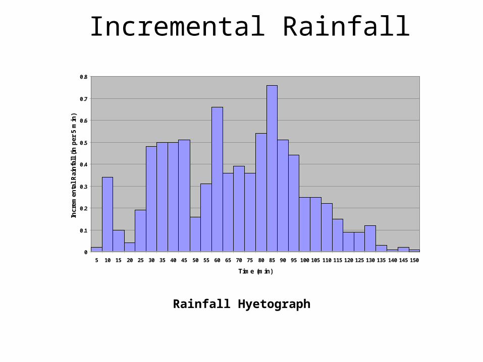
Incremental Rainfall

0

0.1

0.2

0.3

0.4

0.5

0.6

0.7

0.8

5 10 15 20 25 30 35 40 45 50 55 60 65 70 75 80 85 90 95 100 105 110 115 120 125 130 135 140 145 150

Time (min)

Incr

emen

tal

Rai

nfa

ll (

in p

er 5

min

)

Rainfall Hyetograph

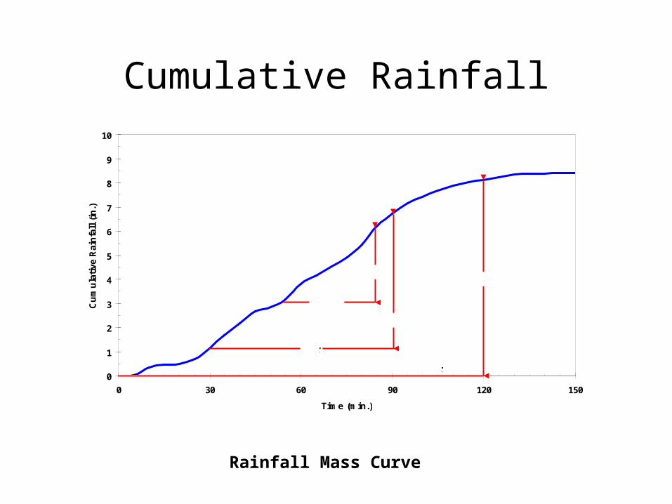
Cumulative Rainfall

0

1

2

3

4

5

6

7

8

9

10

0 30 60 90 120 150

Time (min.)

Cu

mu

lati

ve R

ain

fall

(in

.)

30 min

1 hr

2 hr

3.07 in

5.56 in

8.2 in

Rainfall Mass Curve

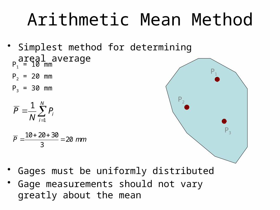
Arithmetic Mean Method• Simplest method for determining areal

averageP1

P2

P3

P1 = 10 mm

P2 = 20 mm

P3 = 30 mm

• Gages must be uniformly distributed• Gage measurements should not vary greatly about

the mean

N

iiPN

P1

1

mmP 203

302010

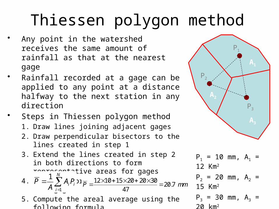
Thiessen polygon method

P1

P2

P3

A1

A2

A3

• Any point in the watershed receives the same amount of rainfall as that at the nearest gage

• Rainfall recorded at a gage can be applied to any point at a distance halfway to the next station in any direction

• Steps in Thiessen polygon method1. Draw lines joining adjacent gages

2. Draw perpendicular bisectors to the lines created in step 1

3. Extend the lines created in step 2 in both directions to form representative areas for gages

4. Compute representative area for each gage

5. Compute the areal average using the following formula

N

iiiPAA

P1

1

P1 = 10 mm, A1 = 12 Km2

P2 = 20 mm, A2 = 15 Km2

P3 = 30 mm, A3 = 20 km2

mmP 7.2047

302020151012

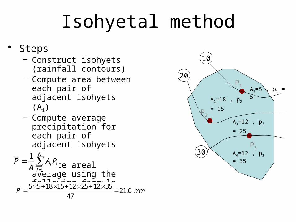
Isohyetal method

P1

P2

P3

10

20

30

• Steps– Construct isohyets (rainfall

contours)– Compute area between

each pair of adjacent isohyets (Ai)

– Compute average precipitation for each pair of adjacent isohyets (pi)

– Compute areal average using the following formula

M

iii pAP

1

A1=5 , p1 = 5

A2=18 , p2 =

15

A3=12 , p3 =

25

A4=12 , p3 = 35

mmP 6.2147

35122512151855

N

iiiPAA

P1

1

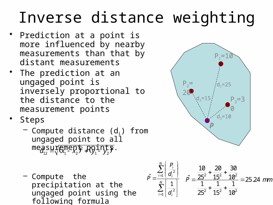
Inverse distance weighting

P1=10

P2= 20

P3=30

• Prediction at a point is more influenced by nearby measurements than that by distant measurements

• The prediction at an ungaged point is inversely proportional to the distance to the measurement points

• Steps– Compute distance (di) from

ungaged point to all measurement points.

– Compute the precipitation at the ungaged point using the following formula

N

i i

N

i i

i

d

d

P

P

12

12

1ˆ

d1=25

d2=15

d3=10

mmP 24.25

10

1

15

1

25

110

30

15

20

25

10

ˆ

222

222

p

2212

2112 yyxxd

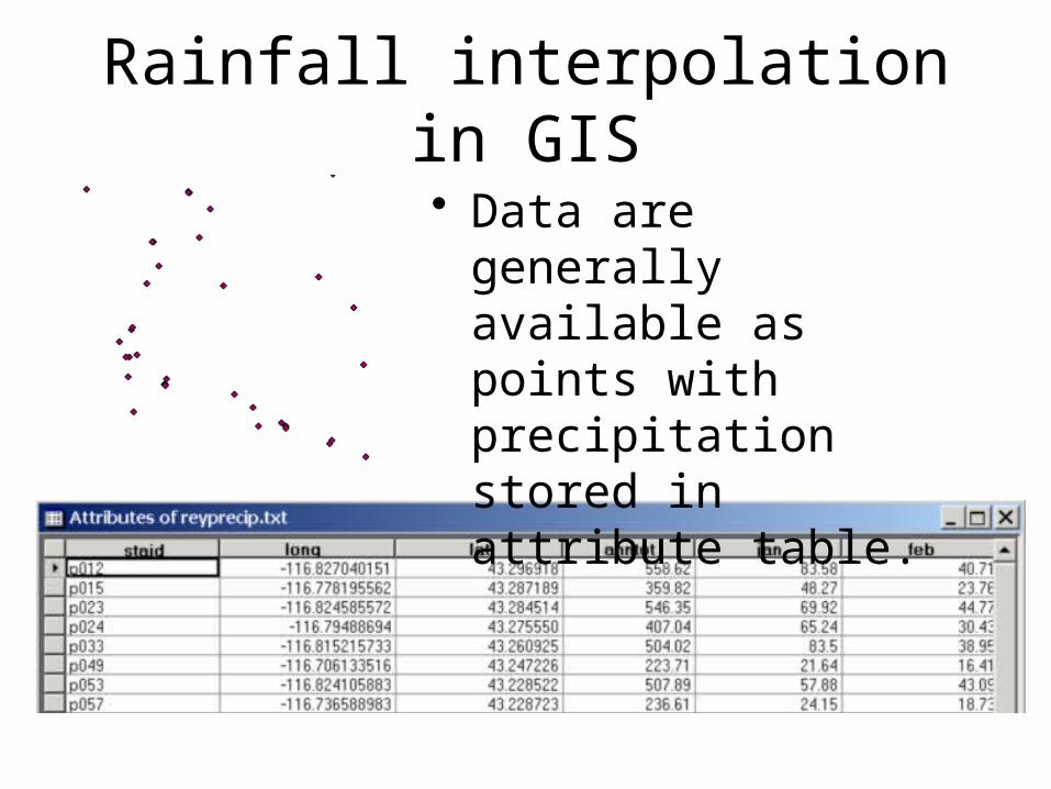
Rainfall interpolation in GIS

• Data are generally available as points with precipitation stored in attribute table.

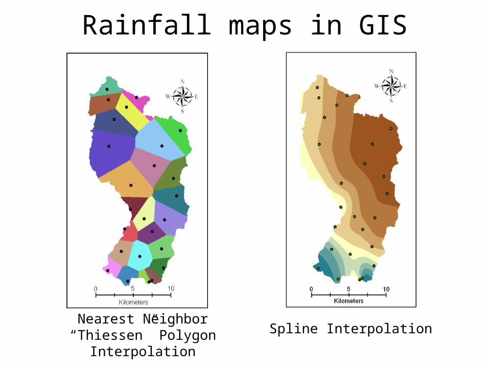
Rainfall maps in GIS

Nearest Neighbor “Thiessen” Polygon Interpolation

Spline Interpolation

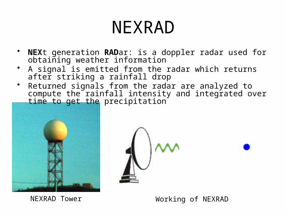
NEXRAD

NEXRAD Tower

• NEXt generation RADar: is a doppler radar used for obtaining weather information

• A signal is emitted from the radar which returns after striking a rainfall drop

• Returned signals from the radar are analyzed to compute the rainfall intensity and integrated over time to get the precipitation

Working of NEXRAD

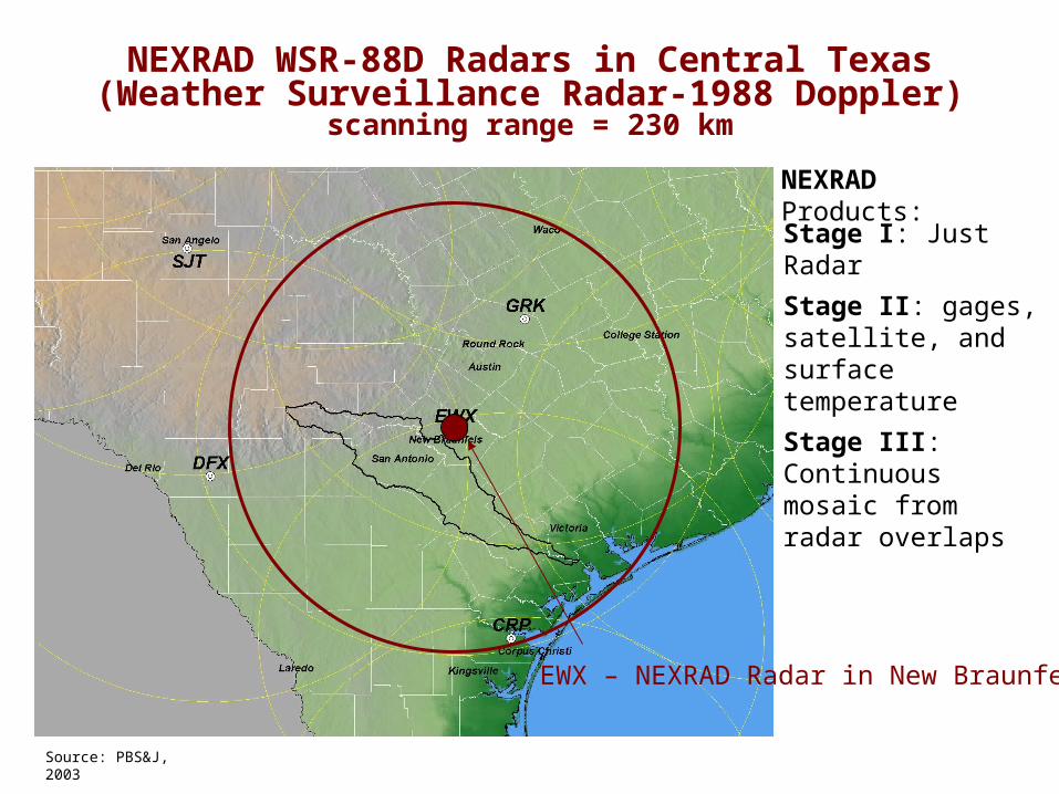
NEXRAD WSR-88D Radars in Central Texas(Weather Surveillance Radar-1988 Doppler)

scanning range = 230 km

Stage I: Just Radar

Stage II: gages, satellite, and surface temperature

Stage III: Continuous mosaic from radar overlaps

NEXRAD Products:

Source: PBS&J, 2003

EWX – NEXRAD Radar in New Braunfels

NEXRAD data

• NOAA’s Weather and Climate Toolkit (JAVA viewer)– http://www.ncdc.noaa.gov/oa/wct/

• West Gulf River Forecast Center– http://www.srh.noaa.gov/wgrfc/

• National Weather Service Precipitation Analysis– http://www.srh.noaa.gov/rfcshare/precip_analysis_new.php