atmospheric pollution research · 2015-06-11 · atmospheric pollution research 2 (2011) ... data...

Atmospheric Pollution Research 2 (2011) 283‐299

Atmospheric Pollution Research

www.atmospolres.com

Assessment of WRF/Chem to simulate sub–Arctic boundary layer characteristics during low solar irradiation using radiosonde, SODAR, and surface data Nicole Mölders 1,2, Huy N.Q. Tran 1,2, Patricia Quinn 3, Kenneth Sassen 1,2, Glenn E. Shaw 1, Gerhard Kramm 1

1 University of Alaska Fairbanks, Geophysical Institute, USA

2 University of Alaska Fairbanks, College of Natural Science and Mathematics, Department of Atmospheric Sciences, 903 Koyukuk Dr., Fairbanks, AK 99775, USA

3 NOAA–PMEL, Ocean Climate Research Division, 7600 Sand Point Way NE, Seattle, WA 98115, USA

ABSTRACT

Data from a Doppler SOund Detection And Ranging (SODAR) device, twice–daily radiosondes, 33 surface meteorological and four aerosol sites were used to assess the ability of the Weather Research and Forecasting model inline coupled with a chemistry package (WRF/Chem) to capture atmospheric boundary layer (ABL) characteristics in Interior Alaska during low solar irradiation (11–01–2005 to 02–28–2006). Biases determined based on all available data from the 33 sites over the entire episode are 1.6 K, 1.8 K, 1.85 m/s, –5 o, and 1.2 hPa for temperature, dewpoint temperature, wind–speed, wind–direction, and sea–level pressure, respectively. The SODAR–data reveal that WRF/Chem over/under–estimates wind–speed in the lower (upper) atmospheric boundary layer. WRF/Chem captures the frequency of low–level jets well, but overestimates the strength of moderate low–level jets. Data from the four aerosol sites suggest large underestimation of PM10, and NO3 at the remote sites and PM2.5 at the polluted site. Difficulty in capturing the temporal evolution of aerosol concentrations coincides with difficulty in capturing sudden temperature changes, underestimation of inversion–strengths and timing of frontal passages. Errors in PM2.5 concentrations strongly relate to temperature errors.

Keywords: WRF/Chem

High–latitudes SODAR

Stable boundary layer Aerosol

Article History: Received: 03 August 2010 Revised: 11 January 2011

Accepted: 14 January 2011

Corresponding Author: Nicole Mölders

Tel: +1‐907‐474‐7910 Fax: +1‐907‐474‐7379

E–mail: [email protected]

© Author(s) 2011. This work is distributed under the Creative Commons Attribution 3.0 License. doi: 10.5094/APR.2011.035 1. Introduction

In air–quality modeling, the accuracy of simulated meteorological fields is of first–order importance. These fields are predicted by the meteorological module of the air–quality model (AQM). Meteorological modules of AQMs were evaluated most thoroughly for mid–latitude and low latitude weather events due to the availability of routine data (Etherton and Santos, 2008; Otkin and Greenwald, 2008; Hong et al., 2009). Validation hardly exists for long–term and seasonally weak–dynamic conditions, governed by stagnant, cold anticyclones with temperature inversions and little precipitation. These conditions, however, are of great interest in high–latitude air–quality studies. These weak–dynamic conditions strongly limit vertical mixing of often–polluted air close to the ground with less polluted air at higher levels of the atmospheric boundary layer (ABL). During late fall and winter (November to February, hereafter called NTF) solar irradiation is low or even not present in high–latitudes. A notable impact on photochemical processes cannot be expected. However, low temperatures and moisture content affect temperature and/or moisture–dependent chemical reactions and particle growth.

AQMs require high accuracy of meteorological quantities as

relative humidity, insolation, air temperature and the presence of liquid cloud particles affect certain chemical reactions directly. The meteorological conditions in the ABL control and/or strongly affect

water–vapor uptake, emission patterns, emitted aerosol–chemical species, chemical transformations and total concentrations of particulate matter (PM). They determine horizontal and vertical transport, turbulent mixing, removal by dry and wet deposition, and the rates at which secondary species and aerosols form. Thus, AQMs have to capture well the basic ABL–characteristics like the 3D–fields of temperature, moisture and wind, thermal stratification, intensity of turbulent mixing, and mixed–layer depth.

To identify the most appropriate physical parameterizations

for air–quality modeling various comparison studies were performed for mid–latitudes (Seaman, 2000). These studies underlined that suitable parameterizations to describe ABL–processes must consider the turbulent fluxes for heat, moisture, and momentum, the exchange processes at the atmosphere–surface interface and shortwave and long–wave radiation fluxes that are all of subgrid–scale with respect to the grid–spacing of AQMs.

The enforcement of air–quality standards and emission

regulations has socio–economic impacts. Thus, scientific guidance provided to policymakers should be based upon well–tested AQMs evaluated for the area in which these models are to be applied. The lack of routine data at both the surface and aloft limits the evaluation of the chemical module of AQMs. Therefore, efforts have been made to evaluate AQMs using data from special field

284 Mölders et al. – Atmospheric Pollution Research 2 (2011) 283‐299

campaigns almost exclusively carried out in highly populated mid–latitude regions (Grell et al., 2000; Becker et al., 2002; McKeen et al., 2007; Eder et al., 2009; Zhang et al., 2009; Wilczak et al., 2009; Djalalova et al., 2010). These evaluated AQMs are often used for other conditions and regions assuming similar quality of performance.

None of the modern AQMs have been developed or assessed

for the sub–Arctic in a sufficient manner. In the sub–Arctic, where the atmosphere can become strongly stable during the long dark nights of NTF, parameterizations often have difficulty capturing the ABL (Hines and Bromwich, 2008; Mölders and Kramm, 2010). Moreover, strong temperature inversions (hereafter called inversions) with strength of up to 50 K/100 m (Bourne et al., 2010) form frequently in valleys. Such inversions cap the air layers close to the ground. In areas strongly polluted by gaseous and particulate matter released by the seasonal combustion for heating, inversions hinder the export of the polluted air into unpolluted or less polluted air layers aloft. These natural atmospheric phenomena cause the accumulation of pollutants, especially of particles with aerodynamic diameters less than 2.5 µm (PM2.5) in Fairbanks, the only major population center in Interior Alaska. Other ABL–phenomena affecting air–quality occurring in Interior Alaska are slope–drainage and channeling winds in mountains.

Our goal is to use SOund Detection And Ranging (SODAR) data,

radiosonde soundings, surface meteorological and aerosol observations to (1) assess WRF/Chem’s (Grell et al., 2005; Peckham et al., 2009) performance in simulating ABL–characteristics for Interior Alaska during NTF, (2) identify model deficits with respect to simulating ABL–characteristics, and (3) assess the potential impact of the current model deficits on air–quality modeling.

2. Methods 2.1. Model setup

WRF/Chem simulates concurrently the meteorological

conditions and chemistry of atmospheric species from emission, through transport and a variety of chemical reactions, to the removal by wet or dry deposition. The Weather Research and Forecasting model (Skamarock et al., 2008) serves as meteorol‐ogical module for WRF/Chem.

We chose the following physical packages that were capable

of capturing Alaska winter conditions well in previous studies (Mölders and Kramm, 2010; Yarker et al., 2010). Cloud– and precipitation–formation processes were simulated by the WRF–Single–Moment six–class scheme that allows for mixed–phase processes and the coexistence of super–cooled water and ice (Hong and Lim, 2006). With a grid–spacing of 4 km, some cumulus clouds are of subgrid–scale. To consider the impact of cumulus convection, despite convection only occurred on a few days during NTF, we used the cumulus–ensemble approach (Grell and Devenyi, 2002). Shortwave radiation was determined by the Goddard two–stream multi–band scheme that considers, among other things, cloud effects and ice–fog. Long–wave radiation was treated with the Rapid Radiative Transfer Model (Mlawer et al., 1997) that considers multiple spectral bands, trace gases, and microphysical species. Turbulent processes in the ABL were determined using a 1D–prognostic TKE–based scheme (Janjic, 2001). However, Monin–Obukhov similarity hypotheses were used to describe the turbulent processes in the atmospheric surface layer, where Zilitinkevich’s thermal roughness–length concept was considered for the underlying viscous sublayer (Janjic, 1994). The exchange of heat and moisture at the land–atmosphere interface was described by Smirnova et al.'s (2000) land–surface model (LSM). The LSM calculates soil–temperature and moisture states including frozen soil physics. Its multi–layer snow model and one–layer vegetation model consider snow and vegetation processes, respectively.

We chose the well–tested chemical setup (Grell et al., 2005; McKeen et al., 2007; Bao et al., 2008) that also performed acceptably for South–Central Alaska (Mölders et al., 2010). Gas–phase chemistry was treated by the chemical mechanism (Stockwell et al., 1990) of the Regional Acid Deposition Model version 2 (Chang et al., 1989). Photolysis frequencies were determined following Madronich (1987) as even at winter solstice Fairbanks experiences 3.7 h of sunlight. The formulation of dry deposition (Wesely, 1989) was modified following Zhang et al. (2003) to treat dry deposition of trace gases more realistically under low temperature conditions. Since the stomata of Alaska vegetation often are still open at –5 °C, the threshold for total stomata closure was lowered accordingly in the LSM and deposition module.

To treat aerosol physics and chemistry we chose the

Secondary ORGanic Aerosol Model (Schell et al., 2001) and Modal Aerosol Dynamics Model for Europe (Ackermann et al., 1998). These modules consider, among other things, inorganic aerosols, secondary organic aerosols, and the wet and dry removal of aerosols.

Some Alaska plant species are photosynthetically active at

temperatures as low as –5 oC. Biogenic emissions of isoprene, monoterpenes, and other volatile organic compounds (VOCs) by plants, and nitrogen emissions by soil were calculated using the Model of Emissions of Gases and Aerosols from Nature (Guenther et al., 1994; Simpson et al., 1995).

Alaska–typical values were taken as vertical profiles of initial

background concentrations (e.g., acetylene, CH3CHO, CH3OOH, CO, ethane, HCHO, HNO3, H2O2, isoprene, NOx, O3, propene, propane, SO2).

2.2. Simulations

The domain of interest for the analysis encompasses

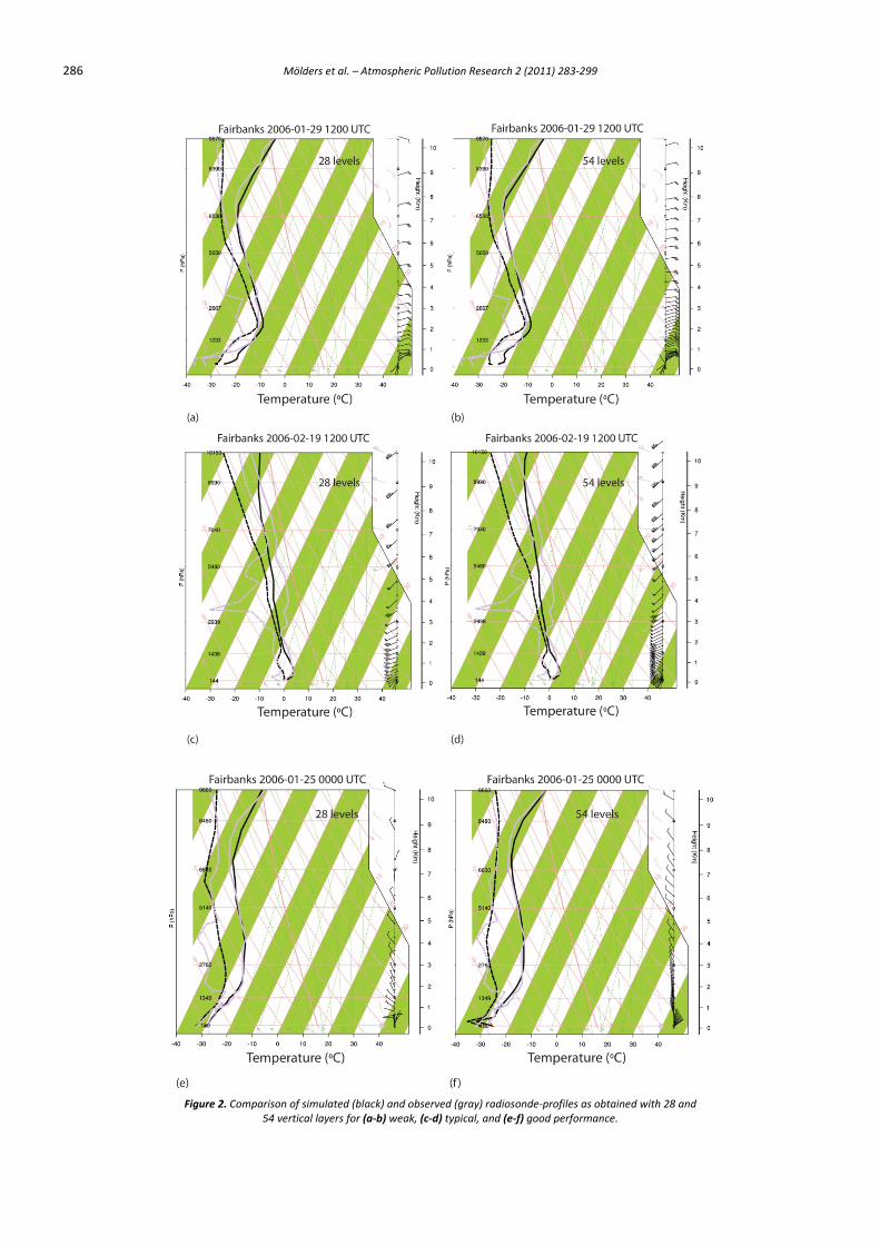
89 600 km2 centered around Fairbanks up to 100 hPa (Figure 1; 80x70 grid–points with a horizontal grid–spacing of 4 km). According to Persson and Warner (1991) an optimal vertical grid–spacing Δzopt for fronts with slopes s of 0.005–0.02 is Δzopt = sΔx. With a horizontal grid–spacing Δx = 4 km, we obtain 0.002–0.08 km. Such a grid–spacing would not permit long–term simulations with WRF/Chem. Mölders and Kramm (2010) already showed for a winter study encompassing Interior Alaska that the performance with higher vertical resolution was not superior to that with 28 levels. Based on sensitivity studies with 54 levels for various days (Figure 2), we came to the same conclusion. During NTF, only 11 fronts were observed in the Interior. The model simulated them all and no gravity–wave–like structures were found in the simulated data. Therefore, we used a vertically stretched grid with 28 layers as a compromise between resolution and computational time to assess WRF/Chem’s long–term performance under low solar irradiance conditions. In the lower troposphere, the tops of the layers were at 8, 16, 64, 113, 219, 343, 478, 632, and 824 m above ground level (AGL).

Anthropogenic emissions stem from the National Emission

Inventory of 2005, and were allocated in space and time according to population density, land–cover, month, weekday, hour, and emission sources. For point–emissions, plume–rise was calculated following Peckham et al. (2009). In accord with the measurements by the Fairbanks North Star Borough, PM was split into ammonium (NH4), carbon, nitrate (NO3), potassium, sodium, and sulfate (SO4). Due to the lack of observational data, we split the total anthropogenic VOC emissions into the various species like alkanes, alkenes, ketones, etc. depending on emission–source types.

The initial conditions for the meteorological, snow and soil

variables were obtained from the 1o x 1o, 6 h–resolution National Centers for Environmental Prediction global final analyses (FNL).

Mölders et al. – Atmospheric Pollution Research 2 (2011) 283‐299 285

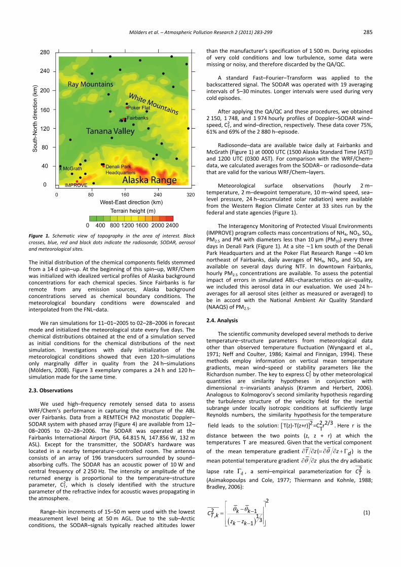
Figure 1. Schematic view of topography in the area of interest. Black crosses, blue, red and black dots indicate the radiosonde, SODAR, aerosol and meteorological sites.

The initial distribution of the chemical components fields stemmed from a 14 d spin–up. At the beginning of this spin–up, WRF/Chem was initialized with idealized vertical profiles of Alaska background concentrations for each chemical species. Since Fairbanks is far remote from any emission sources, Alaska background concentrations served as chemical boundary conditions. The meteorological boundary conditions were downscaled and interpolated from the FNL–data.

We ran simulations for 11–01–2005 to 02–28–2006 in forecast

mode and initialized the meteorological state every five days. The chemical distributions obtained at the end of a simulation served as initial conditions for the chemical distributions of the next simulation. Investigations with daily initialization of the meteorological conditions showed that even 120 h–simulations only marginally differ in quality from the 24 h–simulations (Mölders, 2008). Figure 3 exemplary compares a 24 h and 120 h–simulation made for the same time.

2.3. Observations

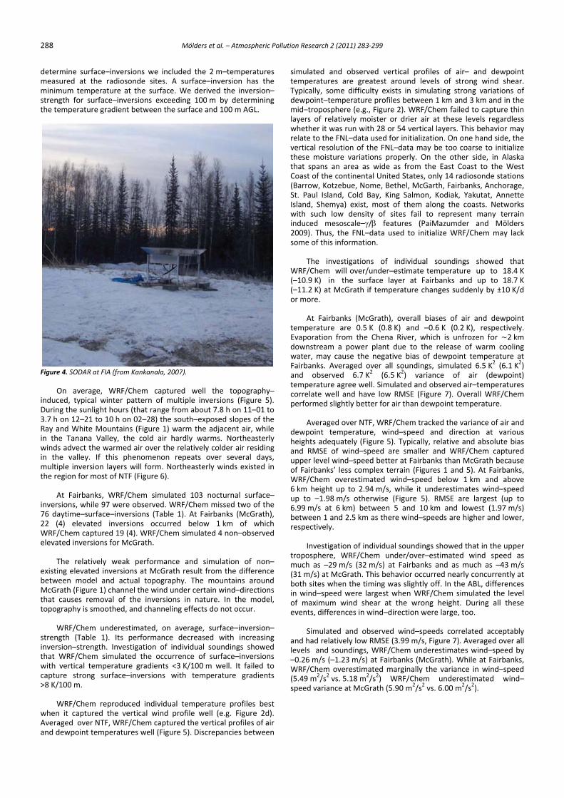
We used high–frequency remotely sensed data to assess

WRF/Chem’s performance in capturing the structure of the ABL over Fairbanks. Data from a REMTECH PA2 monostatic Doppler–SODAR system with phased array (Figure 4) are available from 12–08–2005 to 02–28–2006. The SODAR was operated at the Fairbanks International Airport (FIA, 64.815 N, 147.856 W, 132 m ASL). Except for the transmitter, the SODAR's hardware was located in a nearby temperature–controlled room. The antenna consists of an array of 196 transducers surrounded by sound–absorbing cuffs. The SODAR has an acoustic power of 10 W and central frequency of 2 250 Hz. The intensity or amplitude of the returned energy is proportional to the temperature–structure parameter, CT

2, which is closely identified with the structure parameter of the refractive index for acoustic waves propagating in the atmosphere.

Range–bin increments of 15–50 m were used with the lowest

measurement level being at 50 m AGL. Due to the sub–Arctic conditions, the SODAR–signals typically reached altitudes lower

than the manufacturer’s specification of 1 500 m. During episodes of very cold conditions and low turbulence, some data were missing or noisy, and therefore discarded by the QA/QC.

A standard Fast–Fourier–Transform was applied to the

backscattered signal. The SODAR was operated with 19 averaging intervals of 5–30 minutes. Longer intervals were used during very cold episodes.

After applying the QA/QC and these procedures, we obtained

2 150, 1 748, and 1 974 hourly profiles of Doppler–SODAR wind–speed, CT

2, and wind–direction, respectively. These data cover 75%, 61% and 69% of the 2 880 h–episode.

Radiosonde–data are available twice daily at Fairbanks and

McGrath (Figure 1) at 0000 UTC (1500 Alaska Standard Time [AST]) and 1200 UTC (0300 AST). For comparison with the WRF/Chem–data, we calculated averages from the SODAR– or radiosonde–data that are valid for the various WRF/Chem–layers.

Meteorological surface observations (hourly 2 m–

temperature, 2 m–dewpoint temperature, 10 m–wind speed, sea–level pressure, 24 h–accumulated solar radiation) were available from the Western Region Climate Center at 33 sites run by the federal and state agencies (Figure 1).

The Interagency Monitoring of Protected Visual Environments

(IMPROVE) program collects mass concentrations of NH4, NO3, SO4, PM2.5 and PM with diameters less than 10 µm (PM10) every three days in Denali Park (Figure 1). At a site 1 km south of the Denali Park Headquarters and at the Poker Flat Research Range 40 km northeast of Fairbanks, daily averages of NH4, NO3, and SO4 are available on several days during NTF. In downtown Fairbanks, hourly PM2.5 concentrations are available. To assess the potential impact of errors in simulated ABL–characteristics on air–quality, we included this aerosol data in our evaluation. We used 24 h–averages for all aerosol sites (either as measured or averaged) to be in accord with the National Ambient Air Quality Standard (NAAQS) of PM2.5. 2.4. Analysis

The scientific community developed several methods to derive temperature–structure parameters from meteorological data other than observed temperature fluctuation (Wyngaard et al., 1971; Neff and Coulter, 1986; Kaimal and Finnigan, 1994). These methods employ information on vertical mean temperature gradients, mean wind–speed or stability parameters like the Richardson number. The key to express CT

2 by other meteorological quantities are similarity hypotheses in conjunction with dimensional π–invariants analysis (Kramm and Herbert, 2006). Analogous to Kolmogorov’s second similarity hypothesis regarding the turbulence structure of the velocity field for the inertial subrange under locally isotropic conditions at sufficiently large Reynolds numbers, the similarity hypothesis for the temperature

field leads to the solution: [ ] 2 2/32T(z)‐T(z+r) =C rT . Here r is the

distance between the two points (z, z + r) at which the temperatures T are measured. Given that the vertical component

of the mean temperature gradient ( )∂ ∂ = ∂ ∂ + ΓθT z z d is the

mean potential temperature gradient zθ∂ ∂ plus the dry adiabatic

lapse rate dΓ , a semi–empirical parameterization for 2CT is

(Asimakopoulps and Cole, 1977; Thiermann and Kohnle, 1988; Bradley, 2006):

( )

2

2 1, 1

31

k kCT kz zk k

θ θ⎡ ⎤

−⎢ ⎥−= ⎢ ⎥−⎢ ⎥−⎣ ⎦

(1)


Figure 2. Comparison of simulated (black) and observed (gray) radiosonde‐profiles as obtained with 28 and

54 vertical layers for (a‐b) weak, (c‐d) typical, and (e‐f) good performance.


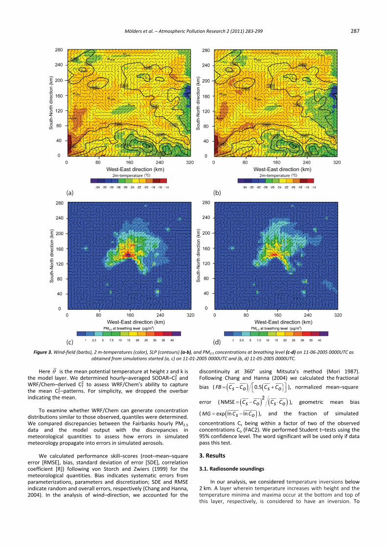
Figure 3. Wind‐field (barbs), 2 m‐temperatures (color), SLP (contours) (a‐b), and PM2.5 concentrations at breathing level (c‐d) on 11‐06‐2005 0000UTC as obtained from simulations started (a, c) on 11‐01‐2005 0000UTC and (b, d) 11‐05‐2005 0000UTC.

Here θ is the mean potential temperature at height z and k is

the model layer. We determined hourly–averaged SODAR–CT2 and

WRF/Chem–derived CT2 to assess WRF/Chem’s ability to capture

the mean CT2–patterns. For simplicity, we dropped the overbar

indicating the mean. To examine whether WRF/Chem can generate concentration

distributions similar to those observed, quantiles were determined. We compared discrepancies between the Fairbanks hourly PM2.5 data and the model output with the discrepancies in meteorological quantities to assess how errors in simulated meteorology propagate into errors in simulated aerosols.

We calculated performance skill–scores (root–mean–square

error [RMSE], bias, standard deviation of error [SDE], correlation coefficient [R]) following von Storch and Zwiers (1999) for the meteorological quantities. Bias indicates systematic errors from parameterizations, parameters and discretization; SDE and RMSE indicate random and overall errors, respectively (Chang and Hanna, 2004). In the analysis of wind–direction, we accounted for the

discontinuity at 360° using Mitsuta’s method (Mori 1987). Following Chang and Hanna (2004) we calculated the fractional

bias ( ( ) ( )0.5FB C C C Cs o s o⎡ ⎤= − +⎣ ⎦ ), normalized mean–square

error ( ( ) ( )2NMSE C C C Cs o s o= − ⋅ ), geometric mean bias

( ( )exp ln lnMG C Cs o= − ), and the fraction of simulated

concentrations Cs being within a factor of two of the observed concentrations Co (FAC2). We performed Student t–tests using the 95% confidence level. The word significant will be used only if data pass this test.

3. Results 3.1. Radiosonde soundings

In our analysis, we considered temperature inversions below

2 km. A layer wherein temperature increases with height and the temperature minima and maxima occur at the bottom and top of this layer, respectively, is considered to have an inversion. To

288

detmeminstrethe

Figu

indDur3.7Rayin winin muthe

inv76 22 WRele

exisbetMcthatop

streinvthawitcap>8

whAveand

8

termine surfaceeasured at thenimum temperength for surfae temperature g

ure 4. SODAR at F

On average,uced, typical wring the sunligh h on 12–21 toy and White Mthe Tanana Vands advect the the valley. If

ultiple inversione region for mos

At Fairbanks,

ersions, while 9daytime–surfa(4) elevated

RF/Chem captuvated inversion The relativel

sting elevated tween model acGrath (Figure 1at causes remopography is smo

WRF/Chem u

ength (Table 1ersion–strengthat WRF/Chem th vertical tempture strong sK/100 m. WRF/Chem r

en it capturederaged over NTd dewpoint tem

e–inversions w radiosonde srature at the suace–inversions gradient betwe

FIA (from Kankan

WRF/Chem winter pattern ht hours (that ro 10 h on 02–28ountains (Figualley, the coldwarmed air ovthis phenome

n layers will forst of NTF (Figur

, WRF/Chem s97 were observce–inversions inversions ored 19 (4). WRFns for McGrath.

y weak perfoinversions at Mand actual top1) channel the woval of the invoothed, and cha

underestimated1). Its performh. Investigationsimulated the perature gradisurface–inversi

reproduced indd the vertical wTF, WRF/Chem mperatures wel

Mölder

we included theites. A surfaceurface. We derexceeding 100en the surface

nala, 2007).

captured welof multiple inange from abo8) the south–exre 1) warm the air hardly waver the relativelenon repeats rm. Northeastere 6).

simulated 103 ved. WRF/Chem(Table 1). At Foccurred belowF/Chem simula.

ormance and sMcGrath result pography. The wind under certversions in natanneling effect

d, on average,mance decreasn of individualoccurrence ofients <3 K/100 ons with tem

dividual tempewind profile wcaptured the vl (Figure 5). Dis

rs et al. – Atmosp

e 2 m–temperae–inversion harived the inver0 m by determand 100 m AGL

l the topogranversions (Figuut 7.8 h on 11–xposed slopes oe adjacent air, arms. Northealy colder air resover several

erly winds exist

nocturnal surm missed two oairbanks (McGw 1 km of wted 4 non–obs

simulation of from the diffemountains ar

tain wind–directure. In the ms do not occur.

, surface–inversed with increl soundings shf surface–inverm well. It fail

mperature grad

rature profileswell (e.g. Figurevertical profiles screpancies bet

heric Pollution Re

atures s the rsion–mining L.

aphy–re 5). –01 to of the while sterly siding days, ted in

rface–of the rath), which erved

non–rence round ctions model,

rsion–easing owed rsions ed to dients

s best e 2d). of air tween

simutempTypicdewmid–layerwhetrelatvertithesethat Coas(BarrSt. PIslanwith indu2009some

WRF(–10(–11or m

tempEvapdowwateFairband tempcorreperfo

dewheighand uppeof FaWRF6 kmup t6.99betwrespe

tropomuc(31 mbothin wof meven

and level–0.2WRF(5.49spee

esearch 2 (2011)

ulated and obsperatures are cally, some difpoint–tempera–troposphere (ers of relatively ther it was run te to the FNL–dcal resolution e moisture varspans an area

st of the continrow, Kotzebue,Paul Island, Cod, Shemya) exsuch low de

ced mesoscale9). Thus, the FNe of this inform The investigaF/Chem will ov.9 K) in the .2 K) at McGra

more. At Fairbanks (perature are 0poration from tnstream a power, may cause banks. Average

observed 6perature agree elate well and ormed slightly b Averaged overpoint temperahts adequatelyRMSE of winder level wind–sairbanks’ less cF/Chem overesm height up to to –1.98 m/s om/s at 6 km)

ween 1 and 2.5ectively. Investigation oosphere, WRF/h as –29 m/s (m/s) at McGrath sites when theind–speed wermaximum windnts, differences Simulated andhad relatively lls and soundin6 m/s (–1.23 mF/Chem overest9 m2/s2 vs. 5.18ed variance at M

283‐299

served verticalgreatest arounfficulty exists inture profiles bee.g., Figure 2). moister or drwith 28 or 54 ata used for inof the FNL–datriations propera as wide as frental United St Nome, Bethel,ld Bay, King Saxist, most of thnsity of sites e–γ/β featureNL–data used t

mation.

tions of indivver/under–estimsurface layer th if temperatu

(McGrath), ove0.5 K (0.8 K) athe Chena Rivewer plant due the negative bed over all sou.7 K2 (6.5 K2) well. Simulatedhave low RMSbetter for air th

NTF, WRF/Cheature, wind–spy (Figure 5). Typd–speed are smpeed better at complex terrainstimated wind–2.94 m/s, whil

otherwise (Figubetween 5 ankm as there w

of individual sou/Chem under/(32 m/s) at Faih. This behavioe timing was slre largest when shear at the in wind–direct

d observed winow RMSE (3.99ngs, WRF/Chemm/s) at Fairbanktimated margin8 m2/s2) WRF/McGrath (5.90 m

l profiles of and levels of stn simulating stetween 1 km aWRF/Chem fairier air at thesevertical layers. itialization. On ta may be too rly. On the othrom the East Ctates, only 14 r, McGarth, Fairalmon, Kodiak,hem along thefail to repres

es (PaiMazumdto initialize WR

vidual soundinmate temperatat Fairbanks ure changes su

erall biases of and –0.6 K (0.er, which is unto the release

bias of dewpoiundings, simula

variance ofd and observedSE (Figure 7). Ohan dewpoint te

em tracked the peed and direpically, relativemaller and WRFairbanks thann (Figures 1 an–speed below le it underestimure 5). RMSE and 10 km and ind–speeds are

undings showed/over–estimateirbanks and asor occurred nealightly off. In thn WRF/Chem swrong heightion were large,

nd–speeds cor9 m/s, Figure 7)m underestimatks (McGrath). Wnally the varian/Chem underm2/s2 vs. 6.00 m

air– and dewptrong wind shtrong variationnd 3 km and inled to capture e levels regardThis behavior one hand side,coarse to initiaher side, in AlaCoast to the Wadiosonde statrbanks, Anchor, Yakutat, Anne coasts. Netwsent many terder and MöldRF/Chem may

ngs showed ture up to 18and up to 18uddenly by ±10

air and dewp.2 K), respectivnfrozen for 2e of warm coont temperaturated 6.5 K2 (6.1f air (dewpod air–temperatuOverall WRF/Chemperature.

variance of air ection at vare and absolute RF/Chem captun McGrath becad 5). At Fairba1 km and ab

mates wind–spare largest (uplowest (1.97 m

e higher and low

d that in the uped wind speed much as –43arly concurrenthe ABL, differensimulated the lt. During all th, too.

related accept. Averaged ovetes wind–speedWhile at Fairbance in wind–sprestimated wim2/s2).

point hear. s of the thin dless may , the alize aska West ions age, ette orks rrain ders lack

that 8.4 K 8.7 K K/d

point vely. 2 km oling e at 1 K2) oint) ures hem

and ious bias ured ause nks, bove peed p to m/s) wer,

pper d as m/s ly at nces evel hese

ably er all d by nks, peed ind–


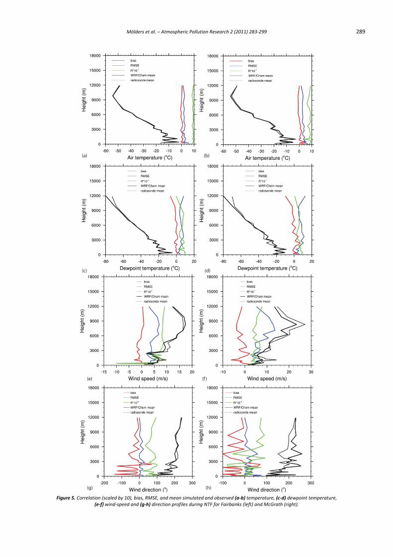
Figure 5. Correlation (scaled by 10), bias, RMSE, and mean simulated and observed (a‐b) temperature, (c‐d) dewpoint temperature,

(e‐f) wind‐speed and (g‐h) direction profiles during NTF for Fairbanks (left) and McGrath (right).


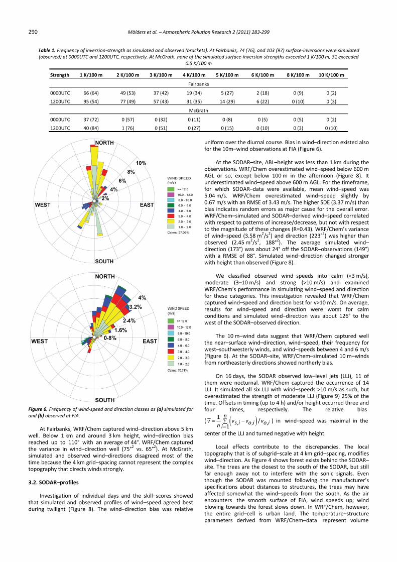
Table 1. Frequency of inversion‐strength as simulated and observed (brackets). At Fairbanks, 74 (76), and 103 (97) surface‐inversions were simulated (observed) at 0000UTC and 1200UTC, respectively. At McGrath, none of the simulated surface‐inversion‐strengths exceeded 1 K/100 m, 31 exceeded

0.5 K/100 m

Strength 1 K/100 m 2 K/100 m 3 K/100 m 4 K/100 m 5 K/100 m 6 K/100 m 8 K/100 m 10 K/100 m

Fairbanks

0000UTC 66 (64) 49 (53) 37 (42) 19 (34) 5 (27) 2 (18) 0 (9) 0 (2)

1200UTC 95 (54) 77 (49) 57 (43) 31 (35) 14 (29) 6 (22) 0 (10) 0 (3)

McGrath

0000UTC 37 (72) 0 (57) 0 (32) 0 (11) 0 (8) 0 (5) 0 (5) 0 (2)

1200UTC 40 (84) 1 (76) 0 (51) 0 (27) 0 (15) 0 (10) 0 (3) 0 (10)

Figure 6. Frequency of wind‐speed and direction classes as (a) simulated for and (b) observed at FIA.

At Fairbanks, WRF/Chem captured wind–direction above 5 km well. Below 1 km and around 3 km height, wind–direction bias reached up to 110° with an average of 44°. WRF/Chem captured the variance in wind–direction well (75°2 vs. 65°2). At McGrath, simulated and observed wind–directions disagreed most of the time because the 4 km grid–spacing cannot represent the complex topography that directs winds strongly.

3.2. SODAR–profiles

Investigation of individual days and the skill–scores showed

that simulated and observed profiles of wind–speed agreed best during twilight (Figure 8). The wind–direction bias was relative

uniform over the diurnal course. Bias in wind–direction existed also for the 10m–wind observations at FIA (Figure 6).

At the SODAR–site, ABL–height was less than 1 km during the

observations. WRF/Chem overestimated wind–speed below 600 m AGL or so, except below 100 m in the afternoon (Figure 8). It underestimated wind–speed above 600 m AGL. For the timeframe, for which SODAR–data were available, mean wind–speed was 5.04 m/s. WRF/Chem overestimated wind–speed slightly by 0.67 m/s with an RMSE of 3.43 m/s. The higher SDE (3.37 m/s) than bias indicates random errors as major cause for the overall error. WRF/Chem–simulated and SODAR–derived wind–speed correlated with respect to patterns of increase/decrease, but not with respect to the magnitude of these changes (R=0.43). WRF/Chem’s variance of wind–speed (3.58 m2/s2) and direction (223°2) was higher than observed (2.45 m2/s2, 188°2). The average simulated wind–direction (173°) was about 24° off the SODAR–observations (149°) with a RMSE of 88°. Simulated wind–direction changed stronger with height than observed (Figure 8).

We classified observed wind–speeds into calm (<3 m/s),

moderate (3–10 m/s) and strong (>10 m/s) and examined WRF/Chem’s performance in simulating wind–speed and direction for these categories. This investigation revealed that WRF/Chem captured wind–speed and direction best for v>10 m/s. On average, results for wind–speed and direction were worst for calm conditions and simulated wind–direction was about 126° to the west of the SODAR–observed direction.

The 10 m–wind data suggest that WRF/Chem captured well

the near–surface wind–direction, wind–speed, their frequency for west–southwesterly winds, and wind–speeds between 4 and 6 m/s (Figure 6). At the SODAR–site, WRF/Chem–simulated 10 m–winds from northeasterly directions showed northerly bias.

On 16 days, the SODAR observed low–level jets (LLJ), 11 of

them were nocturnal. WRF/Chem captured the occurrence of 14 LLJ. It simulated all six LLJ with wind–speeds >10 m/s as such, but overestimated the strength of moderate LLJ (Figure 9) 25% of the time. Offsets in timing (up to 4 h) and/or height occurred three and four times, respectively. The relative bias

( ( )1/, , ,

1

nv v v vs i o i o in i

= −∑=

) in wind–speed was maximal in the

center of the LLJ and turned negative with height. Local effects contribute to the discrepancies. The local

topography that is of subgrid–scale at 4 km grid–spacing, modifies wind–direction. As Figure 4 shows forest exists behind the SODAR–site. The trees are the closest to the south of the SODAR, but still far enough away not to interfere with the sonic signals. Even though the SODAR was mounted following the manufacturer’s specifications about distances to structures, the trees may have affected somewhat the wind–speeds from the south. As the air encounters the smooth surface of FIA, wind speeds up; wind blowing towards the forest slows down. In WRF/Chem, however, the entire grid–cell is urban land. The temperature–structure parameters derived from WRF/Chem–data represent volume


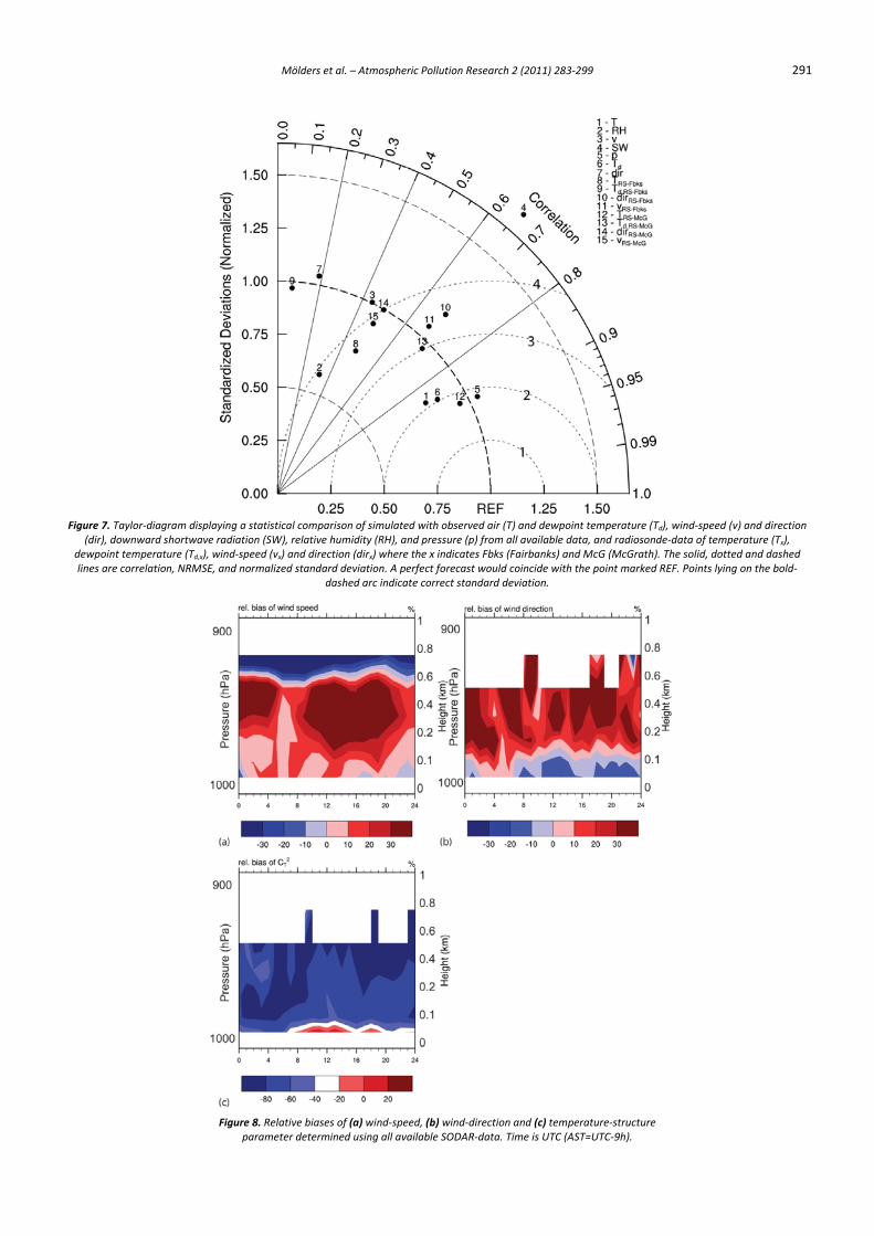
Figure 7. Taylor‐diagram displaying a statistical comparison of simulated with observed air (T) and dewpoint temperature (Td), wind‐speed (v) and direction

(dir), downward shortwave radiation (SW), relative humidity (RH), and pressure (p) from all available data, and radiosonde‐data of temperature (Tx), dewpoint temperature (Td,x), wind‐speed (vx) and direction (dirx) where the x indicates Fbks (Fairbanks) and McG (McGrath). The solid, dotted and dashed lines are correlation, NRMSE, and normalized standard deviation. A perfect forecast would coincide with the point marked REF. Points lying on the bold‐

dashed arc indicate correct standard deviation.

Figure 8. Relative biases of (a) wind‐speed, (b) wind‐direction and (c) temperature‐structure

parameter determined using all available SODAR‐data. Time is UTC (AST=UTC‐9h).


averages of 4 kmx4 km model–layer thickness, while the averaged SODAR–data represents much smaller volumes of same thickness that increase horizontally with increasing height. Thus, our comparison focused mainly on the similarity of pattern.

WRF/Chem reproduced the general features of the CT

2–pattern. However, averaged over all available data, mean CT

2–values (121 K2/m2/3) determined from observations were about three times higher than those determined from simulations (44 K2/m2/3). Overall, RMSE is 190 K2/m2/3.

The mean WRF/Chem–derived (96 K2/m2/3) and observation–

derived (89 K2/m2/3) CT2–values agreed well for wind–speeds

<3 m/s. The negative bias of CT2 grew with increasing wind–speed.

The variance (158 K4/m4/3) was more than twice as high when determined from the observations than simulations (61 K4/m4/3). The large observed variance may relate to aircraft traffic at FIA that causes mixing and vertical exchange of air of different properties.

3.3. Meteorological surface observations

WRF/Chem–simulated meteorological variables and the

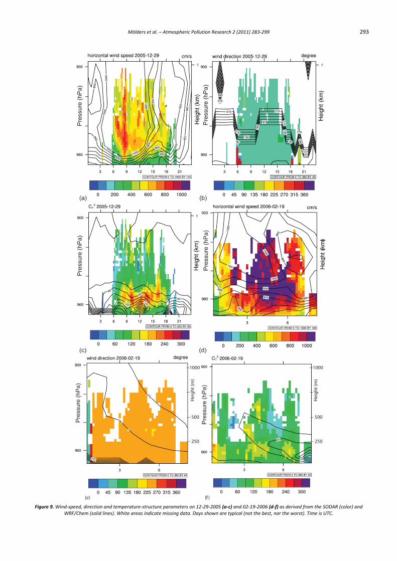
observations at the 33 sites did not differ significantly, and correlations were significant. Averaged over all data, WRF/Chem simulated the NTF–seasonal weather pattern of dewpoint temperature, wind–direction, 24 h–accumulated solar radiation and sea–level pressure (SLP) of Interior Alaska well. Biases in hourly temperature, dewpoint temperature, wind–speed, wind–direction, downward shortwave radiation, and SLP were 1.6 K, 1.8 K, 1.85 m/s, –5°, 9 W/m2, and 1.2 hPa, respectively. Note that the bias of 24 h–accumulated downward shortwave radiation was much larger than 9 W/m2, and strongly depended on the length of daylight (Figure 10).

WRF/Chem captured well the general temporal evolution of

downward shortwave radiation, but overestimated it. As daylight got shorter (longer) the absolute bias decreased (increased). During cloudy periods, initializing every 5th day causes a trend in bias over the 5 d–simulation with too high irradiation at the beginning when clouds spin–up (Figure 10). WRF/Chem starts with zero cloud and precipitation particles on the first day of a simulation. It takes about 3–6 h for clouds to form. Thus, at 0000UTC (1500AST), still enough shortwave radiation exists for most of the time to be affected by potentially too low cloudiness. Initializing 6 h earlier and discarding the first 6 h causes discrepancies between the meteorological and chemical fields (cf. also Figure 3) and was avoided therefore.

WRF/Chem captured well the temporal evolution of air– and

dewpoint temperature, SLP and wind–speed, except for sudden strong (>10 K/d) temperature changes and errors in timing (up to 4 h) of frontal passages (Figure 10). It also performed well outside of frontal passages. During sudden extreme temperature–change events, WRF/Chem failed to capture the full extent of temperature change.

In the Taylor (2001) diagram (Figure 7), the standard deviation

is normalized to its observed value. All available data during the episode were used, i.e. for the radiosonde–data the entire profiles twice a day and for the 33 sites the hourly values. The diagram suggests that WRF/Chem captured the standard deviation of SLP, wind–speed and direction adequately, indicating that the pattern variations are of the right amplitude. WRF/Chem captured the standard deviation of air and dewpoint temperature acceptably, and relative humidity and 24 h–accumulated downward shortwave radiation broadly. For the latter the initialization and differences between the saturation–vapor pressure over water and ice play a role. At the temperatures considered here, saturation with respect to ice exists at a (water) relative humidity as low as 70%.

Relative accuracy was highest for the temperature profile at McGrath, and SLP followed by dewpoint– and air temperature. It was worst for the dewpoint–temperature profile at Fairbanks and wind–direction (Figure 7). The former is due to the open Chena River and the strong water–vapor emissions from Fairbanks that are inert to the observations, but not included in the simulations. These emissions affect the dewpoint temperatures in the lower 1 000 m of the radiosonde profile. The low relative accuracy in wind–direction was due to subgrid–scale wind–channeling effects at many observational sites. The better relative accuracy for the wind–directions for the radiosonde profiles than the 33 sites indicates that WRF/Chem captured vertical–temporal patterns better than temporal pattern at the surface. Accuracy increases with height as local (subgrid–scale) terrain effects loose and synoptic–scale flow patterns gain impact on wind–direction.

The NRMSE of wind–speed was best for the Fairbanks

radiosonde–profile followed by that of McGrath and the 33 sites. This finding indicates difficulty in simulating wind–speed in the ABL related to subgrid–scale topographic effects.

The SDE of temperature, dewpoint temperature, wind–speed,

wind–direction, and SLP amount 5.3 K, 5.1 K, 2.46 m/s, 149°, and 6.9 hPa, respectively. The fact that the SDEs exceeded the biases, suggests that random errors were the major cause for the RMSE.

3.4. Aerosols

A perfect model would have MG, FAC2 and R equal to 1 with

zero FB and NMSE. Since FB and MG measure only the systematic model bias, predictions and observations can be completely out of phase and the evaluation still provides FB=0 or MG=1 due to canceling errors. The NMSE measures the mean relative scatter.

AQMs with fractional biases within ±30%, random scatter

being within a factor of two or three of the mean, and 50% of the predictions falling within a factor of two of the observations are considered to perform well (Chang and Hanna, 2004). The low data density (Table 2) and number of sites may increase errors due to local effects.

WRF/Chem–aerosol simulations for Interior Alaska under low

insolation conditions fall in the lower end of acceptable performance. The simulated maximum PM2.5 concentration is about 6% too low (Table 2). Averaged over all PM2.5 sites and time, WRF/Chem provided 1.2 times higher 24 h–concentrations than observed. However, averaging over data from a remote and a polluted site may be misleading. Simulated and observed PM2.5 agree best at the polluted Fairbanks site. Here, the 24 h–averaged simulated and observed PM2.5–concentrations correlate slightly higher than for the combined data (Table 2). At the Fairbanks site, the overall bias and significant correlation of 24 h–average PM2.5 concentrations were 4.0 µg/m3 and 0.59, respectively.

On average, WRF/Chem underestimated PM10–concentrations

and the maximum PM10–concentration by nearly an order and more than two orders of magnitude, respectively (Table 2). It underestimated the maximum and mean NH4–concentrations by more than an order of magnitude. Typically, SO4–concentrations were simulated 20% too low. The observed SO4–concentration maximum is twice as higher than simulated. WRF/Chem, on average, underestimated NO3–concentrations by two orders of magnitude. Since there are only 16 NO3–data, the weak NO3–performance should not be over–evaluated.

Averaged over the two PM2.5– and SO4–sites, 41% and 50% of

the predictions, respectively, fell within a factor of two. For the low background concentrations at the PM10–, NO3– and NH4–sites, persistence out–performs the forecast (Table 2). Obviously,


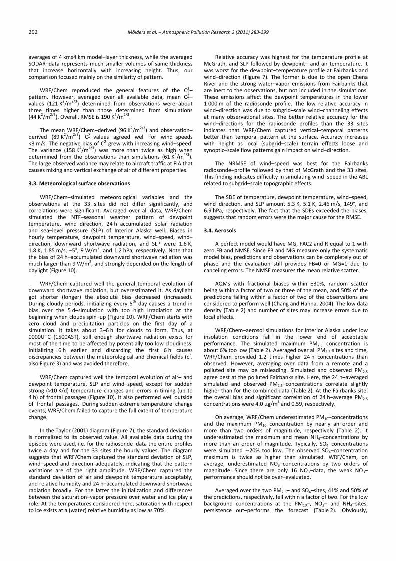
Figure 9. Wind‐speed, direction and temperature‐structure parameters on 12‐29‐2005 (a‐c) and 02‐19‐2006 (d‐f) as derived from the SODAR (color) and

WRF/Chem (solid lines). White areas indicate missing data. Days shown are typical (not the best, nor the worst). Time is UTC.


Figure 10. Temporal evolution of (a) air‐temperature, (b) wind‐speed, (c) 24 h‐accumulated downward shortwave radiation, and (d) pressure averaged over all sites for which data were available. Plots for dewpoint (not shown) and air‐temperatures look similar.

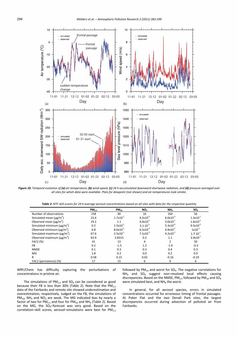
Table 2. NTF skill‐scores for 24 h‐average aerosol concentrations based on all sites with data for the respective quantity

PM2.5 PM10 NO3 NH4 SO4

Number of observations 158 40 16 164 56Simulated mean (µg/m3) 23.4 1.7x10‐1 4.2x10‐4 6.0x10‐3 1.3x10‐1

Observed mean (µg/m3) 19.2 1.1 4.0x10‐2 3.0x10‐1 1.6x10‐1

Simulated minimum (µg/m3) 0.2 1.5x10‐1 5.1⋅10‐5 5.3x10‐9 9.5x10‐2

Observed minimum (µg/m3) 0.8 8.6x10‐2 6.5x10‐4 4.9x10‐3 1x10‐2

Simulated maximum (µg/m3) 67.6 2.5x10‐1 7.1x10‐3 4.2x10‐2 1.7⋅10‐1 Observed maximum (µg/m3) 63.9 3.8315 0.2 1.1 3.9x10‐1

FAC2 (%)

41 13 4 2 50FB 0.2 ‐1.5 1.2 ‐1.9 ‐0.3NMSE 0.1 0.3 0.3 0.4 0.3MG 1.8 0.2 0.0 0.2 0.9R 0.58 0.15 0.02 ‐0.16 ‐0.19FAC2 (persistence) (%) 17 15 6 9 6

WRF/Chem has difficulty capturing the perturbations of concentrations in pristine air.

The simulations of PM2.5 and SO4 can be considered as good

because their FB is less than 30% (Table 2). Note that the PM2.5 data of the Fairbanks and remote site showed underestimation and overestimation, respectively. Judged on the FB, the simulations of PM10, NH4 and NO3 are weak. The MG indicated bias by nearly a factor of two for PM2.5 and four for PM10 and NH4 (Table 2). Based on the MG, the SO4–forecast was very good. Based on the correlation–skill scores, aerosol–simulations were best for PM2.5

followed by PM10 and worst for SO4. The negative correlations for NH4 and SO4 suggest non–resolved local effects causing discrepancies. Based on the NMSE, PM2.5 followed by PM10 and SO4 were simulated best, and NH4 the worst.

In general, for all aerosol species, errors in simulated

concentrations occurred for erroneous timing of frontal passages. At Poker Flat and the two Denali Park sites, the largest discrepancies occurred during advection of polluted air from Fairbanks.


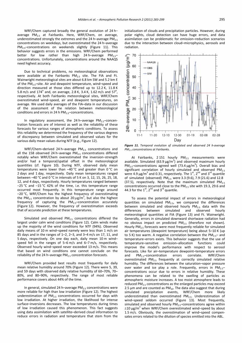
WRF/Chem captured broadly the general evolution of 24 h–average PM2.5 at Fairbanks. Here, WRF/Chem, on average, underestimated strongly the extremes and the 24 h–average PM2.5 concentrations on weekdays, but overestimated the 24 h–average PM2.5–concentrations on weekends slightly (Figure 11). This behavior suggests errors in the emissions. WRF/Chem performed better for low rather than high 24 h–average PM2.5–concentrations. Unfortunately, concentrations around the NAAQS need highest accuracy.

Due to technical problems, no meteorological observations

were available at the Fairbanks PM2.5 site. The FIA and Ft. Wainwright meteorological sites are about 6.8 km SW and 5.2 km E of the PM2.5–site. Air and dewpoint temperature, wind–speed and direction measured at those sites differed up to 12.2 K, 11.8 K 5.8 m/s and 174o and, on average, 2.8 K, 3.4 K, 1.62 m/s and 57o, respectively. At both Fairbanks meteorological sites, WRF/Chem overestimated wind–speed, air and dewpoint temperatures, on average. We used daily averages of the FIA–data in our discussion of the assessment of the relation between meteorological conditions and errors in 24 h PM2.5–concentrations.

In regulatory assessment, the 24 h–average PM2.5–concen‐

tration forecasts are of interest as well as the reliability of these forecasts for various ranges of atmospheric conditions. To assess this reliability we determined the frequency of the various degrees of discrepancy between simulated and observed values for the various daily mean values during NTF (e.g., Figure 12).

WRF/Chem–derived 24 h–average PM2.5 concentrations and

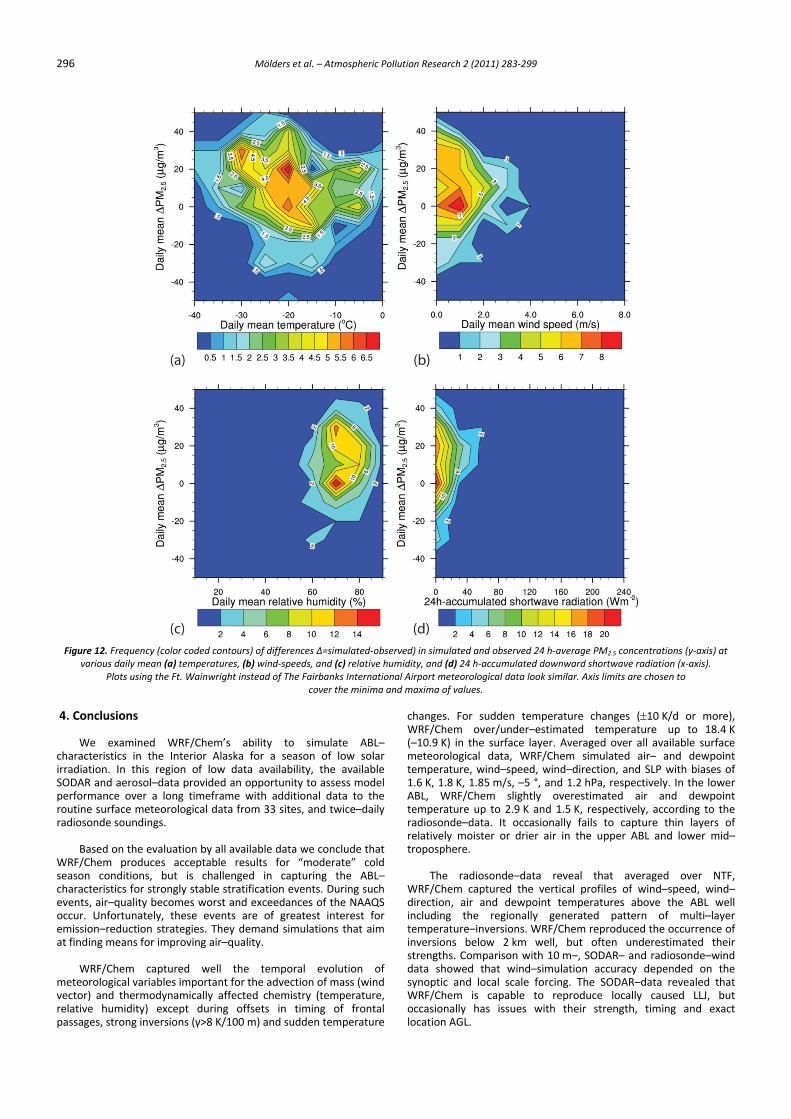
all the 158 observed 24 h–average PM2.5 concentrations differed notably when WRF/Chem overestimated the inversion–strength and/or had a temporal/spatial offset in the meteorological quantities (cf. Figure 10). During NTF, observed daily mean temperatures were lower than –40 °C and greater than 0 °C on 2 days and 1 day, respectively. Daily mean temperatures ranged between –40 °C and 0 °C in intervals of 5 K on 3, 12, 15, 26, 25, 18, 12, and 4 days, respectively. Hourly temperatures ranged between –25 °C and –15 °C 42% of the time, i.e. this temperature range occurred most frequently. In this temperature range around –20 °C, WRF/Chem has the highest frequency of overestimating the PM2.5 concentration by about 20 μg/m

3, but also the highest frequency of capturing the PM2.5–concentration accurately (Figure 12). However, the frequency of overestimation exceeds that of accurate prediction at these temperatures.

Simulated and observed PM2.5 concentrations differed the

largest under calm wind conditions (Figure 12). Calm winds make up the majority of the wind conditions for NTF (94%). Observed daily means of 10 m wind–speed namely were less than 1 m/s on 85 days and in the ranges of 1–2, 2–3, and 3–4 m/s on 17, 11, and 5 days, respectively. On one day each, daily mean 10 m wind–speed fell in the ranges of 5–6 m/s and 6–7 m/s, respectively. Observed hourly wind–speed never exceeded 13 m/s. This means that based on wind conditions one cannot conclude on the reliability of the 24 h–average PM2.5 concentration forecasts.

WRF/Chem provided best results most frequently for daily

mean relative humidity around 70% (Figure 12). There were 5, 39, and 59 days with observed daily relative humidity of 60–70%, 70–80%, and 80–90%, respectively. The range of most reliable performance covers about 44% of the time.

In general, simulated 24 h–average PM2.5 concentrations were

more reliable for high than low irradiation (Figure 12). The highest underestimation of PM2.5 concentrations occurred for days with low irradiation. At higher irradiation, the likelihood for intense surface–inversions decreases. The low temperatures during times of low irradiation caused this phenomenon. This fact suggests using data assimilation with satellite–derived cloud information to reduce errors in radiation and temperature that stem from the

initialization of clouds and precipitation particles. However, during polar nights, cloud detection can have huge errors, and data assimilation can be problematic for emission–reduction scenarios due to the interaction between cloud–microphysics, aerosols and radiation.

Figure 11. Temporal evolution of simulated and observed 24 h‐average PM2.5 concentrations at Fairbanks.

At Fairbanks, 2 151 hourly PM2.5 measurements were

available. Simulated (63.9 µg/m3) and observed maximum hourly PM2.5–concentrations agreed well (73.4 µg/m

3). Overall bias and significant correlation of hourly simulated and observed PM2.5 were 4.9 µg/m3 and 0.31, respectively. The 1st, 2nd and 3rd quantile of simulated (observed) PM2.5 were 3.3 (9.6), 7.9 (21.6) and 12.8 (37.5), respectively. Note that the maximum simulated PM2.5 concentrations occurred close to the PM2.5 site with 19.3, 29.6 and 44.3 for the 1st, 2nd and 3rd quantile.

To assess the potential impact of errors in meteorological

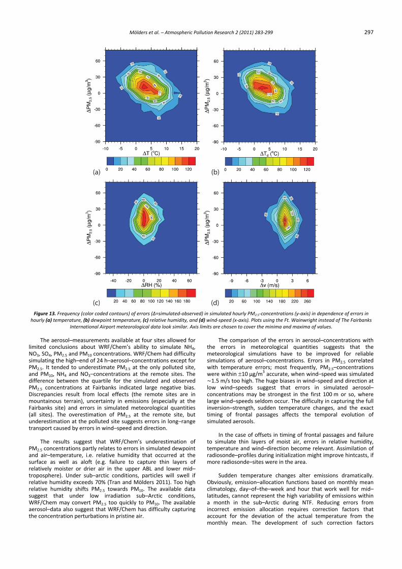
quantities on simulated PM2.5, we compared the differences between simulated and observed hourly PM2.5 data with the differences between simulated and observed hourly meteorological quantities at FIA (Figure 13) and Ft. Wainwright. Generally, errors in simulated downward shortwave radiation had no obvious impact on predicted PM2.5 (therefore not shown). Hourly PM2.5 forecasts were most frequently reliable for simulated air temperatures (dewpoint temperature) being about 5–10 K (up to 5 K) too warm. A negative correlation between the PM2.5– and temperature–errors exists. This behavior suggests that the use of temperature–sensitive emission–allocation functions could improve the model’s performance with respect to aerosol forecasts. Like for air–temperature dewpoint–temperature errors and PM2.5–concentration errors correlate. WRF/Chem overestimated PM2.5 frequently at correctly simulated relative humidity. The differences between the saturation–vapor pressure over water and ice play a role. Frequently, errors in PM2.5–concentrations occur due to errors in relative humidity. These phenomena can be related to the swelling of particles as atmospheric moisture increases. A too moist atmosphere leads to reduced PM2.5 concentrations as the enlarged particles may exceed 2.5 µm and are counted as PM10. The data also suggest that during simulated precipitation events, WRF/Chem more likely underestimated than overestimated PM2.5. Underestimation of wind–speed seldom occurred (Figure 13). Most frequently, simulated and observed hourly PM2.5–concentrations agree within ±10 µg/m3 when WRF/Chem overestimated wind–speed by about 1.5 m/s. Obviously, the overestimation of wind–speed compen‐sates errors related to the dilution of species emitted into the ABL.


Figure 12. Frequency (color coded contours) of differences Δ=simulated‐observed) in simulated and observed 24 h‐average PM2.5 concentrations (y‐axis) at

various daily mean (a) temperatures, (b) wind‐speeds, and (c) relative humidity, and (d) 24 h‐accumulated downward shortwave radiation (x‐axis). Plots using the Ft. Wainwright instead of The Fairbanks International Airport meteorological data look similar. Axis limits are chosen to

cover the minima and maxima of values.

4. Conclusions We examined WRF/Chem’s ability to simulate ABL–

characteristics in the Interior Alaska for a season of low solar irradiation. In this region of low data availability, the available SODAR and aerosol–data provided an opportunity to assess model performance over a long timeframe with additional data to the routine surface meteorological data from 33 sites, and twice–daily radiosonde soundings.

Based on the evaluation by all available data we conclude that

WRF/Chem produces acceptable results for “moderate” cold season conditions, but is challenged in capturing the ABL–characteristics for strongly stable stratification events. During such events, air–quality becomes worst and exceedances of the NAAQS occur. Unfortunately, these events are of greatest interest for emission–reduction strategies. They demand simulations that aim at finding means for improving air–quality.

WRF/Chem captured well the temporal evolution of

meteorological variables important for the advection of mass (wind vector) and thermodynamically affected chemistry (temperature, relative humidity) except during offsets in timing of frontal passages, strong inversions (γ>8 K/100 m) and sudden temperature

changes. For sudden temperature changes (±10 K/d or more), WRF/Chem over/under–estimated temperature up to 18.4 K (–10.9 K) in the surface layer. Averaged over all available surface meteorological data, WRF/Chem simulated air– and dewpoint temperature, wind–speed, wind–direction, and SLP with biases of 1.6 K, 1.8 K, 1.85 m/s, –5 °, and 1.2 hPa, respectively. In the lower ABL, WRF/Chem slightly overestimated air and dewpoint temperature up to 2.9 K and 1.5 K, respectively, according to the radiosonde–data. It occasionally fails to capture thin layers of relatively moister or drier air in the upper ABL and lower mid–troposphere.

The radiosonde–data reveal that averaged over NTF,

WRF/Chem captured the vertical profiles of wind–speed, wind–direction, air and dewpoint temperatures above the ABL well including the regionally generated pattern of multi–layer temperature–inversions. WRF/Chem reproduced the occurrence of inversions below 2 km well, but often underestimated their strengths. Comparison with 10 m–, SODAR– and radiosonde–wind data showed that wind–simulation accuracy depended on the synoptic and local scale forcing. The SODAR–data revealed that WRF/Chem is capable to reproduce locally caused LLJ, but occasionally has issues with their strength, timing and exact location AGL.


Figure 13. Frequency (color coded contours) of errors (Δ=simulated‐observed) in simulated hourly PM2.5‐concentrations (y‐axis) in dependence of errors in

hourly (a) temperature, (b) dewpoint temperature, (c) relative humidity, and (d) wind‐speed (x‐axis). Plots using the Ft. Wainwright instead of The Fairbanks International Airport meteorological data look similar. Axis limits are chosen to cover the minima and maxima of values.

The aerosol–measurements available at four sites allowed for

limited conclusions about WRF/Chem’s ability to simulate NH4, NO3, SO4, PM2.5 and PM10 concentrations. WRF/Chem had difficulty simulating the high–end of 24 h–aerosol–concentrations except for PM2.5. It tended to underestimate PM2.5 at the only polluted site, and PM10, NH4 and NO3–concentrations at the remote sites. The difference between the quartile for the simulated and observed PM2.5 concentrations at Fairbanks indicated large negative bias. Discrepancies result from local effects (the remote sites are in mountainous terrain), uncertainty in emissions (especially at the Fairbanks site) and errors in simulated meteorological quantities (all sites). The overestimation of PM2.5 at the remote site, but underestimation at the polluted site suggests errors in long–range transport caused by errors in wind–speed and direction.

The results suggest that WRF/Chem’s underestimation of

PM2.5 concentrations partly relates to errors in simulated dewpoint and air–temperature, i.e. relative humidity that occurred at the surface as well as aloft (e.g. failure to capture thin layers of relatively moister or drier air in the upper ABL and lower mid–troposphere). Under sub–arctic conditions, particles will swell if relative humidity exceeds 70% (Tran and Mölders 2011). Too high relative humidity shifts PM2.5 towards PM10. The available data suggest that under low irradiation sub–Arctic conditions, WRF/Chem may convert PM2.5 too quickly to PM10. The available aerosol–data also suggest that WRF/Chem has difficulty capturing the concentration perturbations in pristine air.

The comparison of the errors in aerosol–concentrations with the errors in meteorological quantities suggests that the meteorological simulations have to be improved for reliable simulations of aerosol–concentrations. Errors in PM2.5 correlated with temperature errors; most frequently, PM2.5–concentrations were within ±10 µg/m3 accurate, when wind–speed was simulated 1.5 m/s too high. The huge biases in wind–speed and direction at

low wind–speeds suggest that errors in simulated aerosol–concentrations may be strongest in the first 100 m or so, where large wind–speeds seldom occur. The difficulty in capturing the full inversion–strength, sudden temperature changes, and the exact timing of frontal passages affects the temporal evolution of simulated aerosols.

In the case of offsets in timing of frontal passages and failure

to simulate thin layers of moist air, errors in relative humidity, temperature and wind–direction become relevant. Assimilation of radiosonde–profiles during initialization might improve hintcasts, if more radiosonde–sites were in the area.

Sudden temperature changes alter emissions dramatically.

Obviously, emission–allocation functions based on monthly mean climatology, day–of–the–week and hour that work well for mid–latitudes, cannot represent the high variability of emissions within a month in the sub–Arctic during NTF. Reducing errors from incorrect emission allocation requires correction factors that account for the deviation of the actual temperature from the monthly mean. The development of such correction factors


requires examining the temperature–emission relationship at temperatures below –20 °C for all source types.

Our results suggest that WRF/Chem has difficulty in describing

the vertical exchange of heat and matter during strongly stable stratification. Thus, for sub–Arctic air–quality studies the parameterization for strongly stable stratification has to be further–developed. Such further–development requires targeted field campaigns. These campaigns should focus on surface–inversion events with strengths >8 K/100 m and on dissipation of elevated inversions by local wind pattern. Eddy–correlation measurements of temperature, water vapor and wind have to be taken under strongly stable conditions to develop parameterizations that permit simulating the vertical mixing more precisely. SODAR–measurements positioned strategically in potential drainage flows, and regions of potentially stagnant air in combination with temporally (hourly) and highly resolved radiosonde soundings are required. Over complex terrain, measurements at different elevations are beneficial to capture the development of drainage flow and the conditions above and below the surface–inversion.

Model further–development for sub–Arctic applications also

requires increased spatial resolution of surface meteorological and aerosol sites than currently exists. Aerosols should be measured at an hourly rather than daily or every third day basis. Increased spatial and temporal resolution of aerosol measurements will permit assessment of model performance in simulating the aerosol distribution, identifying shortcomings and missing processes, and improving WRF/Chem for low irradiance applications if the underestimation that we found based on the available measurements, is real.

Acknowledgements

We thank J. Fochesatto, T.T. Tran and the anonymous

reviewers for fruitful discussion, P.K. Kankanala for the SODAR–measurements, and the NWS Fairbanks for access to use their site. The Fairbanks North Star Borough (contract LGFEEQ) and NSF (contracts ATM–0630506, ARC0652838) provided financial support. Computational support was provided in part by a grant of HPC–resources from the Arctic Region Supercomputing Center at UAF as part of the Department of Defense High Performance Computing Modernization Program.

References Ackermann, I.J., Hass, H., Memmesheimer, M., Ebel, A., Binkowski, F.S.,

Shankar, U., 1998. Modal aerosol dynamics model for Europe: development and first applications. Atmospheric Environment 32, 2981‐2999.

Asimakopoulos, D.N., Cole, R.S., 1977. An Acoustic sounder for remote probing of the lower atmosphere. Journal of Physics E: Scientific Instruments 10, 47‐50.

Bao, J.W., Michelson, S.A., Persson, P.O.G., Djalalova, I.V., Wilczak, J.M., 2008. Observed and WRF‐simulated low‐level winds in a high‐ozone episode during the Central California ozone study. Journal of Applied Meteorology and Climatology 47, 2372‐2394.

Becker, A., Scherer, B., Memmesheimer, M., Geiß, H., 2002. Studying the city plume of Berlin on 20 July 1998 with three different modelling approaches. Journal of Atmospheric Chemistry 42, 41‐70.

Bourne, S.M., Bhatt, U.S., Zhang, J., Thoman, R., 2010. Surface‐based temperature inversions in Alaska from a climate perspective. Atmospheric Research 95, 353‐366.

Bradley, S., 2006. Atmospheric Acoustic Remote Sensing, CRC Press, Taylor and Francis Group, Boca Raton, 271 pp.

Chang, J. S., Binkowski, F.S., Seaman, N.L.,McHenry, J.N., Samson, P.J., Stockwell, W.R., Walcek, C.J., Madronich, S., Middleton, P.B., Pleim, J.E., Lansford, H.H., 1989. The Regional Acid Deposition Model and Engineering Model. State‐of‐Science/Technology, Report 4, National Acid Precipitation Assessment Program, Washington D.C.

Chang, J.C., Hanna, S.R., 2004. Air quality model performance evaluation. Meteorology and Atmospheric Physics 87, 167‐196.

Djalalova, I., Wilczak, J., McKeen, S., Grell, G., Peckham, S., Pagowski, M., DelleMonache, L., McQueen, J., Tang, Y., Lee, P., McHenry, J., Gong, W., Bouchet, V., Mathur, R., 2010. Ensemble and bias‐correction techniques for air quality model forecasts of surface O3 and PM2.5 during the TEXAQS‐II experiment of 2006. Atmospheric Environment 44, 455‐467.

Eder, B., Kang, D.W., Mathur, R., Pleim, J., Yu, S.C., Otte, T., Pouliot, G., 2009. A performance evaluation of the national air quality forecast capability for the summer of 2007. Atmospheric Environment 43, 2312‐2320.

Etherton, B., Santos, P., 2008. Sensitivity of WRF forecasts for South Florida to initial conditions. Weather and Forecasting 23, 725‐740.

Grell, G.A., Devenyi, D., 2002. A generalized approach to parameterizing convection combining ensemble and data assimilation techniques. Geophysical Research Letters 29, art. no. 1693.

Grell, G.A., Emeis, S., Stockwell, W.R., Schoenemeyer, T., Forkel, R., Michalakes, J., Knoche, R., Seidl, W., 2000. Application of a multiscale, coupled MM5/chemistry model to the complex terrain of the VOTALP valley campaign. Atmospheric Environment 34, 1435‐1453.

Grell, G.A., Peckham, S.E., Schmitz, R., McKeen, S.A., Frost, G., Skamarock, W.C., Eder, B., 2005. Fully coupled "online" chemistry within the WRF model. Atmospheric Environment 39, 6957‐6975.

Guenther, A., Hewitt, C.N., Erickson, D., Fall, R., Geron, C., Graedel, T., Harley, P., Klinger, L., Lerdau, M., Mckay, W.A., Pierce, T., Scholes, B., Steinbrecher, R., Tallamraju, R., Taylor, J., Zimmerman, P., 1995. A global‐model of natural volatile organic compound emissions. Journal of Geophysical Research‐Atmospheres 100, 8873‐8892.

Hines, K.M., Bromwich, D.H., 2008. Development and testing of polar weather research and forecasting (WRF) model. Part I: Greenland ice sheet meteorology. Monthly Weather Review 136, 1971‐1989.

Hong, S.‐Y., Lim, J.‐O.J., 2006. The WRF single‐moment 6‐class microphysics scheme (WSM6). Journal Korean Meteorological Society 42, 129‐151.

Hong, S.‐Y., Sunny Lim, K.‐S., Kim, J.‐H., Jade Lim, J.‐O., Dudhia, J., 2009. Sensitivity study of cloud‐resolving convective simulations with WRF using two bulk microphysical parameterizations:ice‐phase microphysics versus sedimentation effects. Journal of Applied Meteorology and Climatology 48, 61‐76.

Janjic, Z.I., 2001. Nonsingular implementation of the Mellor‐Yamada level 2.5 scheme in the NCEP Meso Model. National Centers for Environmental Prediction Office Note 437, 61pp.

Janjic, Z.I., 1994. The step‐mountain eta coordinate model: further developments of the convection, viscous sublayer, and turbulence closure schemes. Monthly Weather Review 122, 927‐945.

Kaimal, J.C., Finnigan, J.J., 1994. Atmospheric Boundary Layer Flows, Oxford University Press, Oxford, 289pp.

Kankanala, P.K.R., 2007. Doppler Sodar Observations of the Winds and Structure in the Lower Atmosphere over Fairbanks, Alaska. MS Thesis, University of Alaska Fairbanks, 130pp.

Kramm, G., Herbert, F., 2006. The structure functions of the velocity and temperature fields from the perspective of dimensional scaling. Flow Turbulence and Combustion 76, 23‐60.

Madronich, S., 1987. Photodissociation in the atmosphere, 1, actinic flux and the effects of ground reflections and clouds. Journal of Geophysical Research‐Atmospheres 92, 9740‐9752.


McKeen, S., Chung, S.H., Wilczak, J., Grell, G., Djalalova, I., Peckham, S., Gong, W., Bouchet, V., Moffet, R., Tang, Y., Carmichael, G.R., Mathur, R., Yu, S., 2007. Evaluation of several PM2.5 forecast models using data collected during the ICARTT/NEAQS 2004 field study. Journal of Geophysical Research‐Atmospheres 112, art. no. D10S20.

Mlawer, E.J., Taubman, S.J., Brown, P.D., Iacono, M.J., Clough, S.A., 1997. Radiative transfer for inhomogeneous atmospheres: RRTM, a validated correlated‐K model for the longwave. Journal of Geophysical Research‐Atmospheres 102, 16663‐16682.

Mölders, N., Kramm, G., 2010. A case study on wintertime inversions in interior Alaska with WRF. Atmospheric Research 95, 314‐332.

Mölders, N., Porter, S.E., Cahill, C.F., Grell, G.A., 2010. Influence of ship emissions on air quality and input of contaminants in Southern Alaska National Parks and Wilderness areas during the 2006 tourist season. Atmospheric Environment 44, 1400‐1413.

Mölders, N., 2008. Suitability of the Weather Research and Forecasting (WRF) model to predict the June 2005 fire weather for Interior Alaska. Weather and Forecasting 23, 953‐973.

Mori, Y., 1987. Methods for estimating the mean and the standard‐deviation of wind direction. Journal of Climate and Applied Meteorology 26, 1282‐1284.

Neff, W.D., Coulter, R.L., 1986. Acoustic Remote Sensing. In: Lenschow, D.H. (Ed.), Probing the Atmospheric Boundary Layer, American Meteorological Society, Boston, 201‐239.

Otkin, J.A., Greenwald, T.J., 2008. Comparison of WRF model‐simulated and MODIS‐derived cloud data. Monthly Weather Review 136, 1957‐1970.

PaiMazumder, D., Mölders, N., 2009. Theoretical assessment of uncertainty in regional averages due to network density and design. Journal of Applied Meteorology and Climatology 48, 1643‐1666.

Peckham, S.E., Fast, J.D., Schmitz, R., Grell, G.A., Gustafson, W.I., McKeen, S.A., Ghan, S.J., Zaveri, R., Easter, R.C., Barnard, J., Chapman, E., Salzmann, M., Wiedinmyer, C., Freitas, S.R., 2009. WRF/Chem Version 3.1 User’s Guide, p.78.

Persson, P.O.G., Warner, T.T., 1991. Model generation of spurious gravity‐waves due to inconsistency of the vertical and horizontal resolution. Monthly Weather Review 119, 917‐935.

Schell, B., Ackermann, I.J., Hass, H., Binkowski, F.S., Ebel, A., 2001. Modeling the formation of secondary organic aerosol within a comprehensive air quality model system. Journal of Geophysical Research‐Atmospheres 106, 28275‐28293.

Seaman, N.L., 2000. Meteorological modeling for air‐quality assessments. Atmospheric Environment 34, 2231‐2259.

Simpson, D., Guenther, A., Hewitt, C.N., Steinbrecher, R., 1995. Biogenic emissions in Europe 1. estimates and uncertainties. Journal of Geophysical Research‐Atmospheres 100, 22875‐22890.

Skamarock, W.C., Klemp, J.B., Dudhia, J., Gill, D.O., Barker, D.M., Duda, M.G., Huang, X.‐Y., Wang, W., Powers, J.G., 2008. A Description of The Advanced Research WRF Version 3, National Center for Atmospheric Research Boulder, Colorado, USA, 125p.

Smirnova, T.G., Brown, J.M., Benjamin, S.G., Kim, D., 2000. Parameterization of cold‐season processes in the MAPS land‐surface scheme. Journal of Geophysical Research‐Atmospheres 105D, 4077‐4086.

Stockwell, W.R., Middleton, P., Chang, J.S., Tang, X.Y., 1990. The 2nd generation regional acid deposition model chemical mechanism for regional air‐quality modeling. Journal of Geophysical Research‐Atmospheres 95, 16343‐16367.

Taylor, K.E., 2001. Summarizing multiple aspects of model performance in a single diagram. Journal of Geophysical Research‐Atmospheres 106, 7183‐7192.

Thiermann, V., Kohnle, A., 1988 A simple model for the structure constant of temperature fluctuations in the lower atmosphere. Journal of Physics D: Applied Physics 21, 37‐40.

Tran, H.N.Q., Mölders, N., 2011. Investigations on meteorological conditions for elevated PM2.5 in Fairbanks, Alaska. Atmospheric Research 99, 39‐49.

von Storch, H., Zwiers, F.W., 1999. Statistical Analysis in Climate Research, Cambridge University Press, 484pp.

Wesely, M.L., 1989. Parameterization of surface resistances to gaseous dry deposition in regional‐scale numerical models. Atmospheric Environment 23, 1293‐1304.

Wilczak, J.M., Djalalova, I., McKeen, S., Bianco, L., Bao, J.W., Grell, G., Peckham, S., Mathur, R., McQueen, J., Lee, P., 2009. Analysis of regional meteorology and surface ozone during the TEXAQS II field program and an evaluation of the NMM‐CMAQ and WRF‐Chem air quality models. Journal of Geophysical Research‐Atmospheres 114, art. no. D00F14.

Wyngaard, J.C., Izumi, Y., Collins, S.A., Jr., 1971. Behavior of the refractive index structure parameter near the ground. Journal of the Optical Society of America 61, 1646‐1650.

Yarker, M.B., PaiMazumder, D., Cahill, C.F., Dehn, J., Prakash, A., Mölders, N., 2010. Theoretical investigations on potential impacts of high‐latitude volcanic emissions of heat, aerosols and water vapor and their interactions with clouds and precipitation. The Open Atmospheric Science Journal 4, 24‐44.

Zhang, L., Brook, J.R., Vet, R., 2003. A revised parameterization for gaseous dry deposition in air‐quality models. Atmospheric Chemistry and Physics 3, 2067‐2082.

Zhang, Y., Dubey, M.K., Olsen, S.C., Zheng, J., Zhang, R., 2009. Comparisons of WRF/Chem simulations in Mexico City with ground‐based rama measurements during the 2006‐MILAGRO. Atmospheric Chemistry and Physics 9, 3777‐3798.

atmospheric pollution research · 2015-06-11 · atmospheric pollution research 2 (2011) ... data...

Documents