atmospheric correction of remotely sensed images in spatial and transform domain

Priti Tyagi & Udhav Bhosle

International Journal of Image Processing (IJIP), Volume (5) : Issue (5) : 2011 564

Atmospheric Correction of Remotely Sensed Images in Spatial and Transform Domain

Priti Tyagi [email protected] Associate Professor PVPP College of Engineering Mumbai University India

Dr. Udhav Bhosle [email protected] Principal Rajiv Gandhi Institute of Technology Mumbai University India

Abstract

Remotely sensed data is an effective source of information for monitoring changes in land use and land cover. However remotely sensed images are often degraded due to atmospheric effects or physical limitations. Atmospheric correction minimizes or removes the atmospheric influences that are added to the pure signal of target and to extract more accurate information. The atmospheric correction is often considered critical pre-processing step to achieve full spectral information from every pixel especially with hyperspectral and multispectral data. In this paper, multispectral atmospheric correction approaches that require no ancillary data are presented in spatial domain and transform domain. We propose atmospheric correction using linear regression model based on the wavelet transform and Fourier transform. They are tested on Landsat image consisting of 7 multispectral bands and their performance is evaluated using visual and statistical measures. The application of the atmospheric correction methods for vegetation analyses using Normalized Difference Vegetation Index is also presented in this paper.

Keywords: Atmospheric Correction, Multispectral, Spatial Domain, Transform Domain, Vegetation Analyses.

1. INTRODUCTION

The atmosphere influences the amount of electromagnetic energy that is sensed by the detectors of an imaging system and these effects are wavelength dependent. This is particularly true for imaging systems such as Landsat Multispectral Scanner (MSS) and Thematic Mapper (TM) that record data in the visible & near infrared parts of the spectrum. When electromagnetic radiation travels through the atmosphere, it may be absorbed or scattered by the constituent particles of the atmosphere. Atmospheric absorption affects mainly the visible and infrared bands. It reduces the solar radiance within the absorption bands of the atmospheric gases. Atmospheric scattering is important only in the visible and near infrared regions. Scattering of radiation by the constituent gases and aerosols in the atmosphere causes degradation of the remotely sensed images. Most noticeably, the solar radiation scattered by the atmosphere towards the sensor without first reaching the ground produces a hazy appearance of the image. This effect is particularly severe in the blue end of the visible spectrum due to the stronger Rayleigh scattering for shorter wavelength radiation. Atmospheric absorption has multiplicative effect & atmospheric scattering has additive effect on the data.

Several different Atmospheric Scattering or haze removal techniques have been developed for use with digital remotely sensed data. Most of the methods use various atmospheric transmission models, in situ field data, or require specific targets to be present in the image. [7] [8] [9]. Major limitation with these sophisticated techniques is that they require information other than digital Image data. [e.g., path radiance and (or) atmospheric transmission at several locations within the image area collected during satellite’s overflight. Ideally, a method that uses in situ or ground



truth information is most accurate in terms of correcting for atmospheric haze effects. However most of the users work with remotely sensed data that has already been collected. Most of the time only data available is the image itself. Image-based radiometric correction methods are simple and effective as they require no ancillary data to estimate the path radiance and sensor offset terms. Hence we propose image based atmospheric correction methods which donot require any information about the camera, Image acquisition and imaging conditions. Eight methods wherein, three methods (Spatial domain) namely Standard Dark Object Subtraction Technique, Improved Dark Object Subtraction Technique and Linear Regression Method, along with five methods in transform domain namely Wavelet Thresholding, Homomorphic filtering, DCT, Wavelet Regression and Fourier Regression are presented in this paper along with performance evaluation of each method. Results are assessed statistically and compared with each other.

The rest of this paper is organized as follows: Section 2 describes Image based atmospheric correction methods in spatial domain wherein Section 3 describes proposed Transform Domain methods. Section 4 gives details of application of the atmospheric correction methods for vegetation analyses using NDVI method. In section 5 we present the results based on visual and statistical measures. Finally section 6 concludes the paper.

2 : IMAGE BASED ATMOSPHERIC CORRECTION METHODS (SPATIAL DOMAIN METHODS)

2.1 Simple Dark Object Subtraction Method Dark object subtraction Technique removes the effects of scattering from the image data. It requires only the information contained in the digital image data. It derives the corrected DN (Digital Number) values solely from the digital data with no outside information[3].

Dark-object subtraction (DOS) is a widely used method of reducing haze within an image and is done for each band individually. It is assumed that there are pixels within each band of a multispectral image that have very low or no reflectance on the ground, and that the difference between the brightness value of these pixels and zero is due to haze. This per-band estimated difference is subtracted from each band of the image. Most dark object subtraction technique assumes that there is a high probability that there are atleast a few pixels within an image which should be black (0% Reflectance) [2]. This assumption is made because in a single band there are large number of pixels (Landsat MSS single band images- over 7 million pixels and Landsat TM single band images- over 45 million pixels). Thus there are some shadows due to topography or clouds in the image where pixels should be completely dark. Ideally, the imaging system should not detect any radiance at these shadow locations and a DN of zero should be assigned to them. However because of atmospheric scattering, the imaging system records a non zero DN value at these supposedly dark shadowed pixel locations. This represents the DN value that must be subtracted from the particular spectral band to remove first order scattering component. Haze DN value is directly selected from the DN frequency Histogram of a digital Image. A different constant is used for each spectral Band with a different set of constants used from image to image. Histogram of given spectral Bands, particularly in the visible spectrum will offset towards higher DN values by some amount due to scattering. There is usually very sharp increase in the number of pixels at some non zero DN or Gray Level X. This DN value is the amount of Haze in that particular Band. Haze DN value is subtracted from the respective spectral Band. 2.2 : Improved Dark Object Subtraction Technique The technique of Dark object haze correction is further improved in this method. [2][3] DN value selected for haze removal using standard dark object subtraction technique may not conform to a realistic relative atmospheric scattering model. Hence problems are encountered in the analysis stage if the digital multispectral image data is haze corrected using the standard Dark object subtraction technique. This lack of conformity may cause the data to be



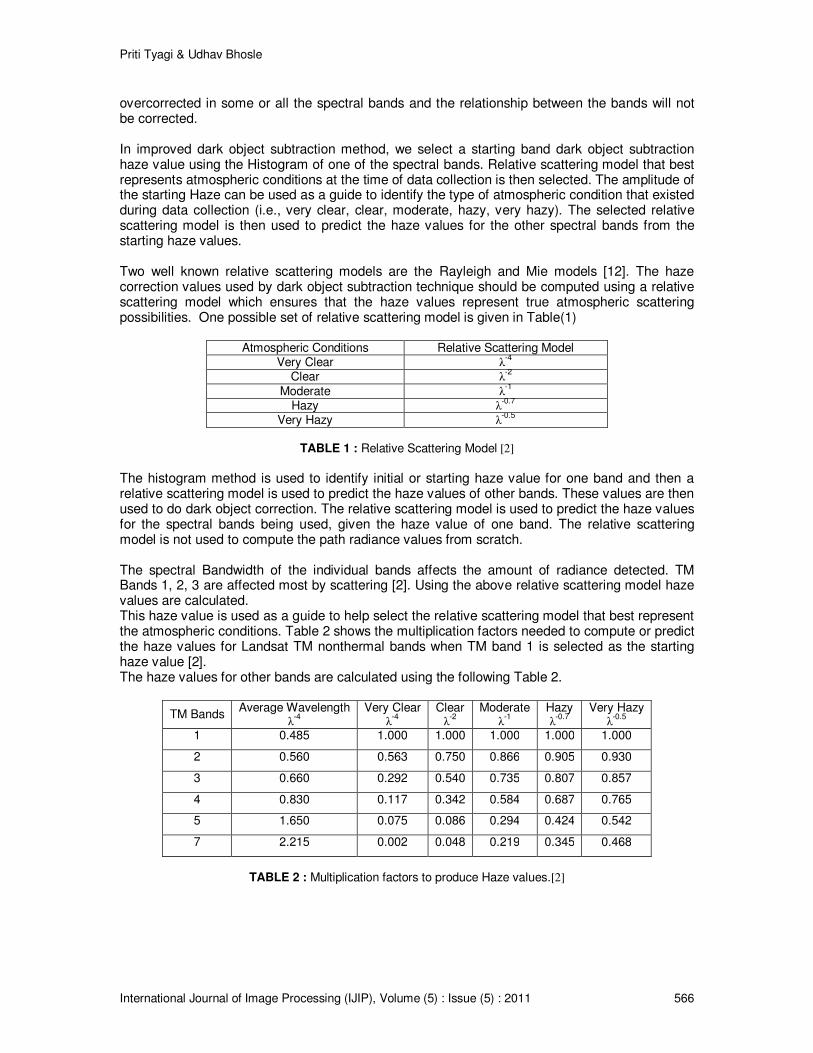
overcorrected in some or all the spectral bands and the relationship between the bands will not be corrected. In improved dark object subtraction method, we select a starting band dark object subtraction haze value using the Histogram of one of the spectral bands. Relative scattering model that best represents atmospheric conditions at the time of data collection is then selected. The amplitude of the starting Haze can be used as a guide to identify the type of atmospheric condition that existed during data collection (i.e., very clear, clear, moderate, hazy, very hazy). The selected relative scattering model is then used to predict the haze values for the other spectral bands from the starting haze values. Two well known relative scattering models are the Rayleigh and Mie models [12]. The haze correction values used by dark object subtraction technique should be computed using a relative scattering model which ensures that the haze values represent true atmospheric scattering possibilities. One possible set of relative scattering model is given in Table(1)

Atmospheric Conditions Relative Scattering Model Very Clear λ-4

Clear λ-2

Moderate λ-1

Hazy λ-0.7

Very Hazy λ-0.5

TABLE 1 : Relative Scattering Model [2]

The histogram method is used to identify initial or starting haze value for one band and then a relative scattering model is used to predict the haze values of other bands. These values are then used to do dark object correction. The relative scattering model is used to predict the haze values for the spectral bands being used, given the haze value of one band. The relative scattering model is not used to compute the path radiance values from scratch. The spectral Bandwidth of the individual bands affects the amount of radiance detected. TM Bands 1, 2, 3 are affected most by scattering [2]. Using the above relative scattering model haze values are calculated. This haze value is used as a guide to help select the relative scattering model that best represent the atmospheric conditions. Table 2 shows the multiplication factors needed to compute or predict the haze values for Landsat TM nonthermal bands when TM band 1 is selected as the starting haze value [2]. The haze values for other bands are calculated using the following Table 2.

TM Bands Average Wavelength

λ-4

Very Clear λ-4

Clear λ-2

Moderate λ-1

Hazy λ-0.7

Very Hazy λ-0.5

1 0.485 1.000 1.000 1.000 1.000 1.000

2 0.560 0.563 0.750 0.866 0.905 0.930

3 0.660 0.292 0.540 0.735 0.807 0.857

4 0.830 0.117 0.342 0.584 0.687 0.765

5 1.650 0.075 0.086 0.294 0.424 0.542

7 2.215 0.002 0.048 0.219 0.345 0.468

TABLE 2 : Multiplication factors to produce Haze values.[2]



2.3 Regression Line Method

Linear Regression Model The regression intersection method of minimizing the effect of the atmosphere provides absolute results from the image data without the use of ancillary data. The method does not require any information or assumptions about the scene, atmospheric conditions or sensor calibrations. The method generally involves calculation of regression lines for a number of surface materials of contrasting spectral properties. The regression line method (RLM) determines a 'best fit' line for multispectral plots of pixels within homogenous cover types. Ideally, the intersection of lines must represent a point of zero ground reflectance since this is the only point at which radiometric values of two spectrally different materials can be safe. If no atmospheric scattering has taken place, the intersection of the line would be expected to pass through the origin. The slope of the plot is proportional to the ratio of the reflective material. However, the lines will, in reality, intersect the x and y axis producing two offset values. These brightness values represent the amount of bias caused by atmospheric scattering. Crippen (1987) recommends the collection of a series of training areas resulting in many regression lines intersecting in two dimensional spaces at the same point using training sets to represent homogeneous land cover types [10]. The relative values generated by regression method tend to be more reliable. However, many new high-resolution satellites provide data which is spectrally and spatially different from Landsat derived data.

General Linear Models

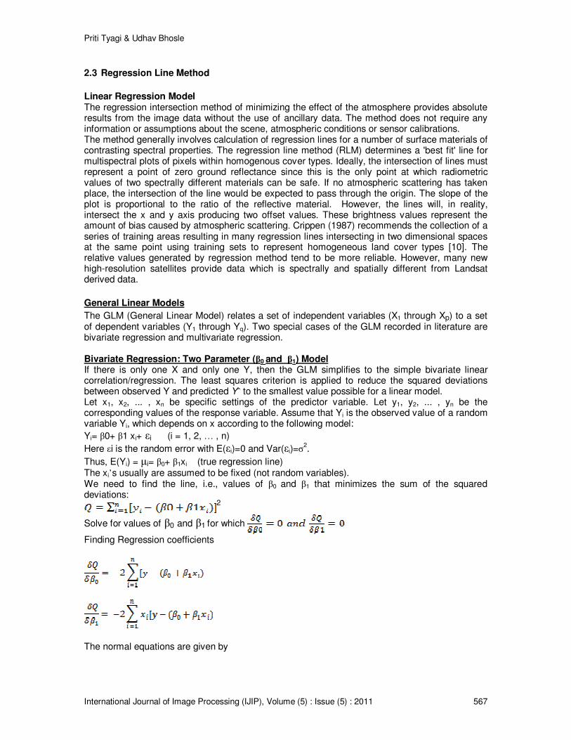
The GLM (General Linear Model) relates a set of independent variables (X1 through Xp) to a set of dependent variables (Y1 through Yq). Two special cases of the GLM recorded in literature are bivariate regression and multivariate regression. Bivariate Regression: Two Parameter (β0 and β1) Model If there is only one X and only one Y, then the GLM simplifies to the simple bivariate linear correlation/regression. The least squares criterion is applied to reduce the squared deviations between observed Y and predicted Yˆ to the smallest value possible for a linear model. Let x1, x2, ... , xn be specific settings of the predictor variable. Let y1, y2, ... , yn be the corresponding values of the response variable. Assume that Yi is the observed value of a random variable Yi, which depends on x according to the following model:

Yi= β0+ β1 xi+ εi (i = 1, 2, … , n)

Here εi is the random error with E(εi)=0 and Var(εi)=σ2.

Thus, E(Yi) = µi= β0+ β1xi (true regression line) The xi’s usually are assumed to be fixed (not random variables). We need to find the line, i.e., values of β0 and β1 that minimizes the sum of the squared deviations:

2

Solve for values of β0 and β1 for which

Finding Regression coefficients

The normal equations are given by



nβ0 + β1 = β0 + β1 =

Finding solution to Normal Equations we get

The coefficient "β0" is the Y-intercept, and " β1" is the slope, the average amount of change in Y per unit change in X. Algorithm for Regression Line Method Regression line method (RLM) suggested here uses one-independent variable regression model described in previous section for estimation of path radiance. The band values, for which correction coefficient is to be determined, regressed against higher spectral bands over homogeneous area. The band to be corrected is plotted on y axis and estimated y intercept is considered as correction coefficient as it is assumed that it equals zero-ground radiance. Threshold for mask to select homogeneous area is determined using histogram of band 5.

• TM Band 5 data is corrected by Improved dark object subtraction method.

• TM Band 4 values are corrected using RLM where Band 5 values are repeated on the independent variable’s axis.

• RLM is again applied to correct Band 3, Band 2 and Band 1, using band 5 as independent variable.

3 Tranform Domain Methods

3.1 Wavelet Thresholding Method As a consequence of atmosphere on remotely sensed images, the images are corrupted by blur and noise. Here, we assume that the image degradation can be described by a linear space-invariant blurring operator and additive Gaussian noise.

To remove atmospheric effects without excessive smoothing of important details, a denoising algorithm needs to be spatially adaptive. The wavelet representation, due to its sparsity, edge detection and multiresolution properties, naturally facilitates such spatially adaptive noise filtering.

Discrete Wavelet Transform

The discrete wavelet analysis is a two channel digital filter bank (composed of the lowpass and the highpass filters), iterated on the lowpass output. The lowpass filtering yields an approximation of a signal (at a given scale), while the highpass (more precisely, bandpass) filtering yields the details that constitute the difference between the two successive approximations. A family of wavelets is then associated with the bandpass, and a family of scaling functions with the lowpass filters. Mallat has introduced a fast, pyramidal filter bank algorithm [Mallat89b] for computing the coefficients of the orthogonal wavelet representation; later it was generalized for the biorthogonal case. This algorithm, is in literature usually referred to as the discrete wavelet transform (DWT).



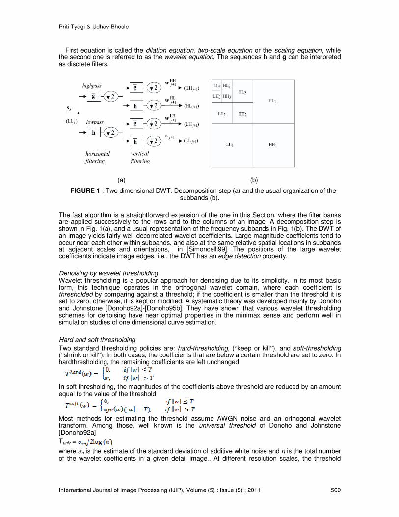
First equation is called the dilation equation, two-scale equation or the scaling equation, while the second one is referred to as the wavelet equation. The sequences h and g can be interpreted as discrete filters.

(a) (b)

FIGURE 1 : Two dimensional DWT. Decomposition step (a) and the usual organization of the subbands (b).

The fast algorithm is a straightforward extension of the one in this Section, where the filter banks are applied successively to the rows and to the columns of an image. A decomposition step is shown in Fig. 1(a), and a usual representation of the frequency subbands in Fig. 1(b). The DWT of an image yields fairly well decorrelated wavelet coefficients. Large-magnitude coefficients tend to occur near each other within subbands, and also at the same relative spatial locations in subbands at adjacent scales and orientations, in [Simoncelli99]. The positions of the large wavelet coefficients indicate image edges, i.e., the DWT has an edge detection property.

Denoising by wavelet thresholding Wavelet thresholding is a popular approach for denoising due to its simplicity. In its most basic form, this technique operates in the orthogonal wavelet domain, where each coefficient is thresholded by comparing against a threshold; if the coefficient is smaller than the threshold it is set to zero, otherwise, it is kept or modified. A systematic theory was developed mainly by Donoho and Johnstone [Donoho92a]-[Donoho95b]. They have shown that various wavelet thresholding schemes for denoising have near optimal properties in the minimax sense and perform well in simulation studies of one dimensional curve estimation.

Hard and soft thresholding

Two standard thresholding policies are: hard-thresholding, (“keep or kill”), and soft-thresholding (“shrink or kill”). In both cases, the coefficients that are below a certain threshold are set to zero. In hardthresholding, the remaining coefficients are left unchanged

In soft thresholding, the magnitudes of the coefficients above threshold are reduced by an amount equal to the value of the threshold

Most methods for estimating the threshold assume AWGN noise and an orthogonal wavelet transform. Among those, well known is the universal threshold of Donoho and Johnstone [Donoho92a]

Tuniv =

where σn is the estimate of the standard deviation of additive white noise and n is the total number of the wavelet coefficients in a given detail image.. At different resolution scales, the threshold



differs only in the constant factor that is related to the number of the coefficients in a given subband.

ALGORITHM

1) Decompose multispectral Landsat TM Image into seven Bands. 2) Consider band 1. Apply discrete wavelet transform to band 1 of the multispectral image. 3) Perform soft thresholding by applying threshold tn = σ √2log(n) to the decomposed band

1 in the multispectral image. 4) Find Inverse DWT of the thresholded image. 5) Repeat steps (2) to (6) for other TM Bands. 6) Concatenate band TM2, TM3, TM4 to see the output image.

3.2 Wavelet Regression

Let and ψ be, respectively, a father and mother wavelet [13] that generate the following complete orthonormal set in L

2[0, 1]:

,

Ψ ,

for integers j ≥ J0 and k, where J0 is fixed. Any function f ∈L

2 [0, 1] may be expanded as

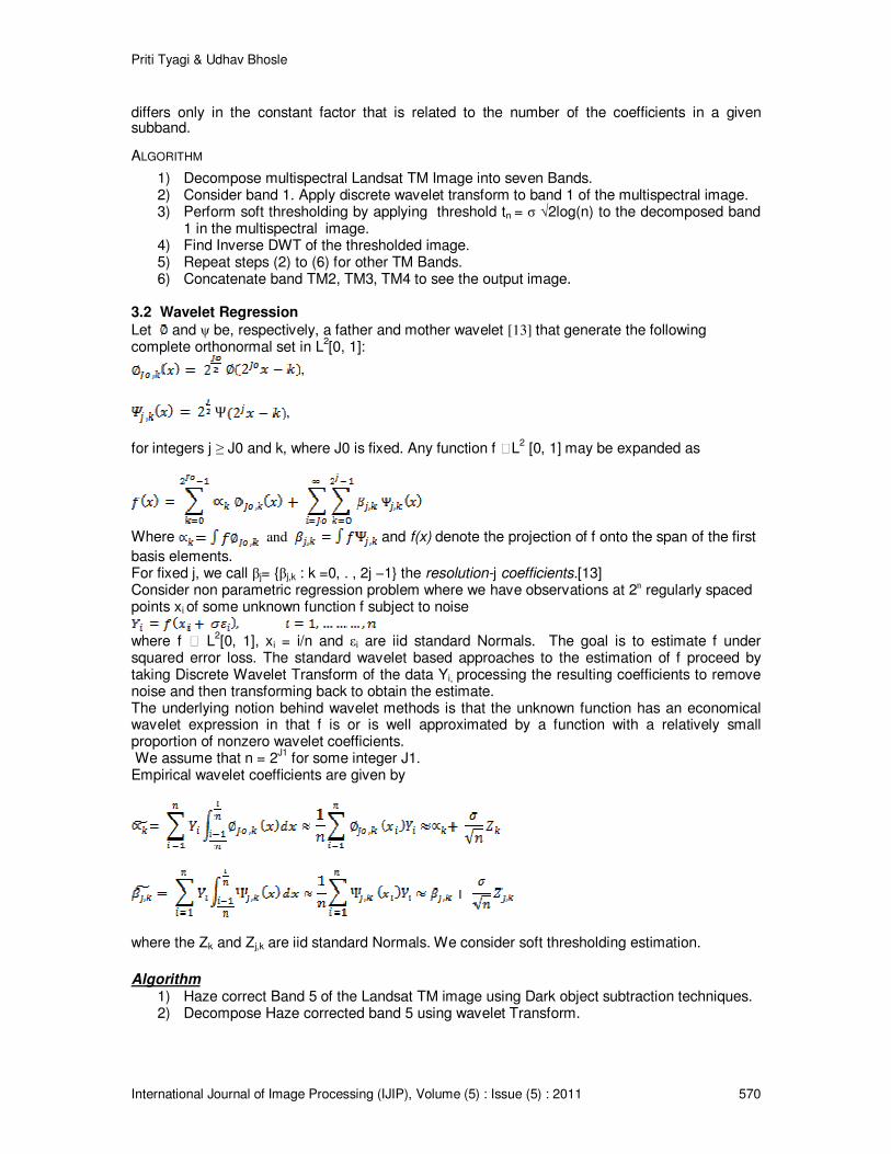
Where and and f(x) denote the projection of f onto the span of the first

basis elements. For fixed j, we call βj= {βj,k : k =0, . , 2j −1} the resolution-j coefficients.[13] Consider non parametric regression problem where we have observations at 2n regularly spaced points xi of some unknown function f subject to noise

where f ∈ L

2[0, 1], xi = i/n and εi are iid standard Normals. The goal is to estimate f under

squared error loss. The standard wavelet based approaches to the estimation of f proceed by taking Discrete Wavelet Transform of the data Yi, processing the resulting coefficients to remove noise and then transforming back to obtain the estimate. The underlying notion behind wavelet methods is that the unknown function has an economical wavelet expression in that f is or is well approximated by a function with a relatively small proportion of nonzero wavelet coefficients. We assume that n = 2

J1 for some integer J1.

Empirical wavelet coefficients are given by

where the Zk and Zj,k are iid standard Normals. We consider soft thresholding estimation.

Algorithm

1) Haze correct Band 5 of the Landsat TM image using Dark object subtraction techniques. 2) Decompose Haze corrected band 5 using wavelet Transform.



3) Perform soft thresholding by applying threshold tn = σ √2log(n) to the decomposed band 5 in the multispectral image.

4) Apply discrete wavelet transform to band 1 of the multispectral image. 5) Threshold decomposed band 1 using soft thresholding. 6) Regress decomposed (DWT) and thresholded band1 to the multiresoution band 5 data

obtained in step (3) using Linear least squares Regression Equation. 7) Find Inverse DWT of the Regressed image. 8) Repeat steps (4) to (7) for other TM Bands. 9) Concatenate band TM2, TM3, TM4 to see the output image.

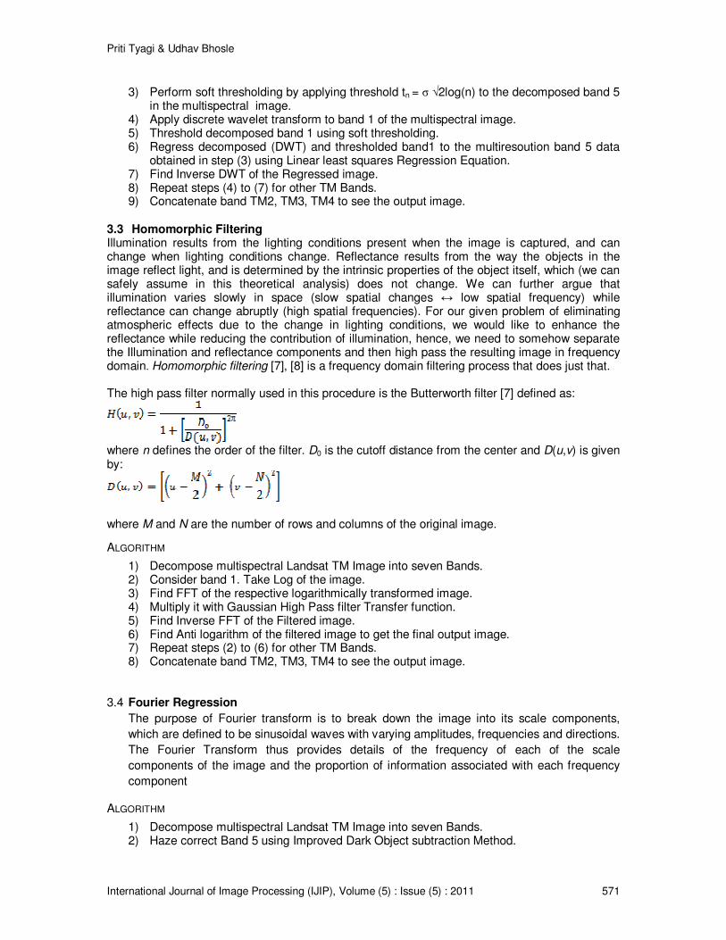
3.3 Homomorphic Filtering Illumination results from the lighting conditions present when the image is captured, and can change when lighting conditions change. Reflectance results from the way the objects in the image reflect light, and is determined by the intrinsic properties of the object itself, which (we can safely assume in this theoretical analysis) does not change. We can further argue that illumination varies slowly in space (slow spatial changes ↔ low spatial frequency) while reflectance can change abruptly (high spatial frequencies). For our given problem of eliminating atmospheric effects due to the change in lighting conditions, we would like to enhance the reflectance while reducing the contribution of illumination, hence, we need to somehow separate the Illumination and reflectance components and then high pass the resulting image in frequency domain. Homomorphic filtering [7], [8] is a frequency domain filtering process that does just that. The high pass filter normally used in this procedure is the Butterworth filter [7] defined as:

where n defines the order of the filter. D0 is the cutoff distance from the center and D(u,v) is given by:

where M and N are the number of rows and columns of the original image.

ALGORITHM

1) Decompose multispectral Landsat TM Image into seven Bands. 2) Consider band 1. Take Log of the image. 3) Find FFT of the respective logarithmically transformed image. 4) Multiply it with Gaussian High Pass filter Transfer function. 5) Find Inverse FFT of the Filtered image. 6) Find Anti logarithm of the filtered image to get the final output image. 7) Repeat steps (2) to (6) for other TM Bands. 8) Concatenate band TM2, TM3, TM4 to see the output image.

3.4 Fourier Regression

The purpose of Fourier transform is to break down the image into its scale components,

which are defined to be sinusoidal waves with varying amplitudes, frequencies and directions.

The Fourier Transform thus provides details of the frequency of each of the scale

components of the image and the proportion of information associated with each frequency

component

ALGORITHM

1) Decompose multispectral Landsat TM Image into seven Bands. 2) Haze correct Band 5 using Improved Dark Object subtraction Method.



3) Find FFT of the Haze corrected Image. 4) Multiply it with Butterworth High Pass filter Transfer function. 5) Consider band 1. Find FFT of the image. 6) Multiply it with High Pass filter Transfer function. 7) Regress the image obtained in step (6) against the image data obtained in step(4) using

Linear regression equations. 8) Find Inverse FFT of the Regressed band 1 image. 9) Repeat steps (5) to (8) for other TM Bands. 10) Concatenate band TM2, TM3, TM4 (false color composite) to see the output image.

3.5 Atmospheric Correction of Multispectral Data using DCT A discrete Cosine Transform (DCT) expresses a sequence of finitely many data points in terms of a sum of cosine functions oscillating at different frequencies. The DCT does a better job of concentrating energy into lower order coefficients for image data. For most images, after transformation the majority of signal energy is carried by just a few of the low order DCT coefficients. These coefficients can be more finely quantized than the higher order coefficients. Many higher order coefficients may be quantized to 0. Formulae for DCT and inverse DCT are as given below:

In the formulas, F(u,v) is the two-dimensional NxN DCT. u,v,x,y = 0,1,2,...N-1. x,y are spatial coordinates in the sample domain. u, v are frequency coordinates in the transform domain. C(u), C(v) = 1/(square root (2)) for u, v = 0. C(u), C(v) = 1 otherwise.

ALGORITHM

1) Decompose multispectral Landsat TM Image into seven Bands. 2) Consider band 1. Find DCT of the image. 3) DCT coefficient at zero frequency is made zero. 4) Find Inverse DCT of the image. 5) Repeat steps (2) to (6) for other TM Bands. 6) Concatenate band TM2, TM3, TM4 to see the output image.

4 : NDVI METHOD FOR VEGETATION ANALYSES One of the applications of the atmospheric correction methods discussed in this paper is Vegetation analysis. Satellite Image processing can be increasingly used in examination of land use and land cover change. NDVI can be very useful in generation of land use/land cover classification. Ratio indices such as the normalized difference vegetation index (NDVI), of Rouse et al. (1973), use various ratios of red and near-infrared bands to determine presence of vegetation. One of the functions of this method is to detect vegetation and plant refreshments and is capable of monitoring those levels in different ages.

NDVI represents the amount of green vegetation and is calculated from reflected red and near infra red light.

NDVI = (NIR - red) / (NIR + red)



NDVI ranges are usually between -1 to 1. Water, snow and clouds or any other nonvegetated scene is represented by negative number. Low positive number near zero indicates rock and bare soil, which reflect near infra red and red at the same level. Increasingly positive number indicates greener vegetation [6]. However, the NDVI is also influenced by sun angle changes and are affected by soil background to the point that they are as sensitive to soil darkening as to vegetation development [4].

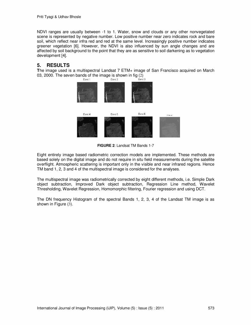
5. RESULTS The image used is a multispectral Landsat 7 ETM+ image of San Francisco acquired on March 03, 2000. The seven bands of the image is shown in fig (2)

FIGURE 2: Landsat TM Bands 1-7

Eight entirely image based radiometric correction models are implemented. These methods are based solely on the digital image and do not require in situ field measurements during the satellite overflight. Atmospheric scattering is important only in the visible and near infrared regions. Hence TM band 1, 2, 3 and 4 of the multispectral image is considered for the analyses.

The multispectral image was radiometrically corrected by eight different methods, i.e. Simple Dark object subtraction, Improved Dark object subtraction, Regression Line method, Wavelet Thresholding, Wavelet Regression, Homomorphic filtering, Fourier regression and using DCT.

The DN frequency Histogram of the spectral Bands 1, 2, 3, 4 of the Landsat TM image is as shown in Figure (3).



(a) (b)

(c) (d)

FIGURE 3: Landsat TM Bands and its corresponding Histogram (a) TM1, (b) TM 2, (c) TM 3, (d) TM 4

In Simple Dark Object Subtraction Method DN Haze value selected from the DN frequency histogram of an image is shown in Table (3)

TM 1 TM 2 TM 3 TM 4

54 35 25 8

TABLE 3 : Haze DN values

This Haze DN value is subtracted from the respective spectral band. The original and the corrected images (composite band 2, 3 and 4) obtained after this is shown in fig (5a) and fig (5b) respectively. This relative normalization method assumes that the effects of haze are distributed evenly across the entire image, which may or may not be the case. This is a good initial adjustment, but there may be problems analyzing the data unless one of five atmospheric scattering models (scaled from very clear to very hazy) is chosen in addition to a dark-object haze value. In Improved Dark object Subtraction Method, the starting haze value selected from TM Band 1 using histogram method is 54. The starting DN haze value must not overpredict the values for other bands. The predicted haze value for TM bands 1, 2, 3, and 4 are shown below.

Haze DN Value

TM 1 TM 2 TM 3 TM 4

54 40.5 29.16 18.468

TABLE 4: Haze DN values

These values were generated using the clear relative scattering model factors shown in Table 2.The image obtained after haze correction is shown in Figure (5c).

As seen from DN haze values (Table 4 and Table 5) TM Band1 is most affected by atmospheric scattering and the value gradually decreases with the bands. Hence we consider that TM band 5



can be used as a reference image to validate the results based on visual analyses as no reference image is available in Absolute Radiometric Correction.

The original and the corrected version of the multispectral image using RLM method is shown in Fig (5d).

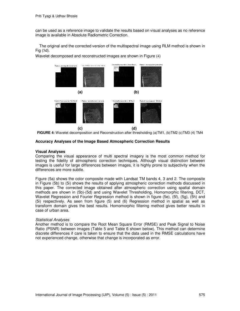
Wavelet decomposed and reconstructed images are shown in Figure (4)

(a) (b)

(c) (d)

FIGURE 4: Wavelet decomposition and Reconstruction after thresholding (a)TM1, (b)TM2 (c)TM3 (4) TM4

Accuracy Analyses of the Image Based Atmospheric Correction Results

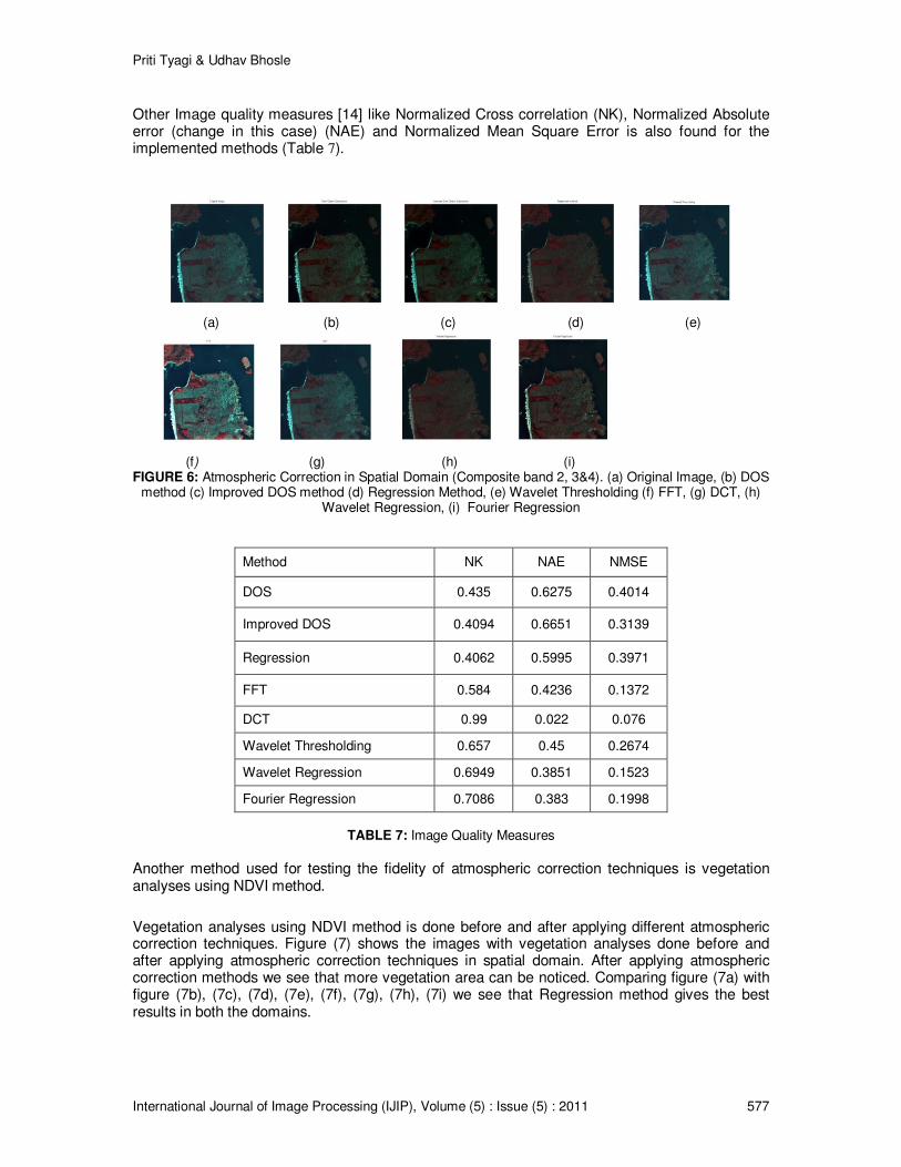
Visual Analyses Comparing the visual appearance of multi spectral imagery is the most common method for testing the fidelity of atmospheric correction techniques. Although visual distinction between images is useful for large differences between images, it is highly prone to subjectivity when the differences are more subtle. Figure (5a) shows the color composite made with Landsat TM bands 4, 3 and 2. The composite in Figure (5b) to (5i) shows the results of applying atmospheric correction methods discussed in this paper. The corrected image obtained after atmospheric correction using spatial domain methods are shown in (5b)-(5d) and using Wavelet Thresholding, Homomorphic filtering, DCT, Wavelet Regression and Fourier Regression method is shown in figure (5e), (5f), (5g), (5h) and (5i) respectively. As seen from figure (5) and (6) Regression method in spatial as well as transform domain gives the best results. Homomorphic filtering method gives better results in case of urban area.

Statistical Analyses Another method is to compare the Root Mean Square Error (RMSE) and Peak Signal to Noise Ratio (PSNR) between images (Table 5 and Table 6 shown below). This method can determine discrete differences if care is taken to ensure that the data used in the RMSE calculations have not experienced change, otherwise that change is incorporated as error.



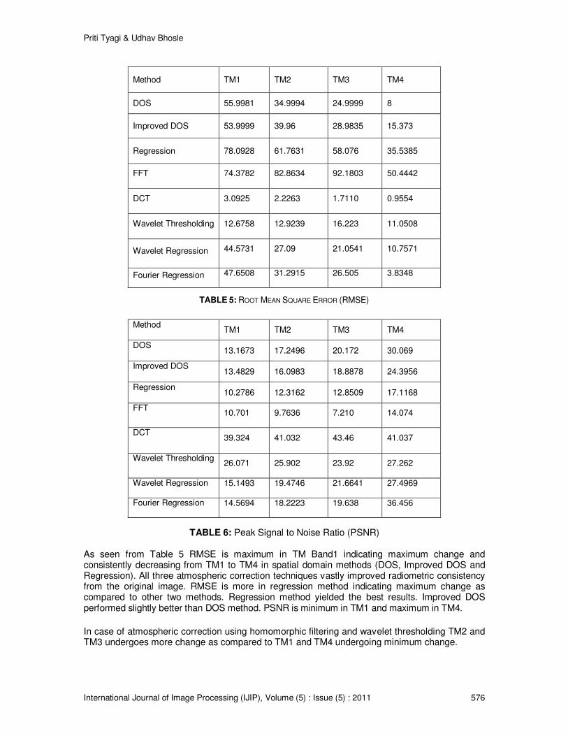
Method TM1 TM2 TM3 TM4

DOS 55.9981 34.9994 24.9999 8

Improved DOS 53.9999 39.96 28.9835 15.373

Regression 78.0928 61.7631 58.076 35.5385

FFT 74.3782 82.8634 92.1803 50.4442

DCT 3.0925 2.2263 1.7110 0.9554

Wavelet Thresholding 12.6758 12.9239 16.223 11.0508

Wavelet Regression 44.5731 27.09 21.0541 10.7571

Fourier Regression 47.6508 31.2915 26.505 3.8348

TABLE 5: ROOT MEAN SQUARE ERROR (RMSE)

Method

TM1 TM2 TM3 TM4

DOS 13.1673 17.2496 20.172 30.069

Improved DOS 13.4829 16.0983 18.8878 24.3956

Regression 10.2786 12.3162 12.8509 17.1168

FFT 10.701 9.7636 7.210 14.074

DCT 39.324 41.032 43.46 41.037

Wavelet Thresholding 26.071 25.902 23.92 27.262

Wavelet Regression 15.1493 19.4746 21.6641 27.4969

Fourier Regression 14.5694 18.2223 19.638 36.456

TABLE 6: Peak Signal to Noise Ratio (PSNR)

As seen from Table 5 RMSE is maximum in TM Band1 indicating maximum change and consistently decreasing from TM1 to TM4 in spatial domain methods (DOS, Improved DOS and Regression). All three atmospheric correction techniques vastly improved radiometric consistency from the original image. RMSE is more in regression method indicating maximum change as compared to other two methods. Regression method yielded the best results. Improved DOS performed slightly better than DOS method. PSNR is minimum in TM1 and maximum in TM4.

In case of atmospheric correction using homomorphic filtering and wavelet thresholding TM2 and TM3 undergoes more change as compared to TM1 and TM4 undergoing minimum change.



Other Image quality measures [14] like Normalized Cross correlation (NK), Normalized Absolute error (change in this case) (NAE) and Normalized Mean Square Error is also found for the implemented methods (Table 7).

(a) (b) (c) (d) (e)

(f) (g) (h) (i) FIGURE 6: Atmospheric Correction in Spatial Domain (Composite band 2, 3&4). (a) Original Image, (b) DOS

method (c) Improved DOS method (d) Regression Method, (e) Wavelet Thresholding (f) FFT, (g) DCT, (h) Wavelet Regression, (i) Fourier Regression

Method NK NAE NMSE

DOS 0.435 0.6275 0.4014

Improved DOS 0.4094 0.6651 0.3139

Regression 0.4062 0.5995 0.3971

FFT 0.584 0.4236 0.1372

DCT 0.99 0.022 0.076

Wavelet Thresholding 0.657 0.45 0.2674

Wavelet Regression 0.6949 0.3851 0.1523

Fourier Regression 0.7086 0.383 0.1998

TABLE 7: Image Quality Measures

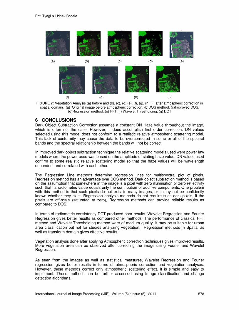
Another method used for testing the fidelity of atmospheric correction techniques is vegetation analyses using NDVI method.

Vegetation analyses using NDVI method is done before and after applying different atmospheric correction techniques. Figure (7) shows the images with vegetation analyses done before and after applying atmospheric correction techniques in spatial domain. After applying atmospheric correction methods we see that more vegetation area can be noticed. Comparing figure (7a) with figure (7b), (7c), (7d), (7e), (7f), (7g), (7h), (7i) we see that Regression method gives the best results in both the domains.



(a) (b) (c) (d) (e)

(f) (g) (h) (i)

FIGURE 7: Vegetation Analysis (a) before and (b), (c), (d) (e), (f), (g), (h), (i) after atmospheric correction in spatial domain. (a) Original image before atmospheric correction, (b)DOS method, (c)Improved DOS,

(d)Regression method. (e) FFT, (f) Wavelet Thresholding, (g) DCT

6 CONCLUSIONS Dark Object Subtraction Correction assumes a constant DN Haze value throughout the image, which is often not the case. However, it does accomplish first order correction. DN values selected using this model does not conform to a realistic relative atmospheric scattering model. This lack of conformity may cause the data to be overcorrected in some or all of the spectral bands and the spectral relationship between the bands will not be correct. In improved dark object subtraction technique the relative scattering models used were power law models where the power used was based on the amplitude of stating haze value. DN values used confirm to some realistic relative scattering model so that the haze values will be wavelength dependent and correlated with each other.

The Regression Line methods determine regression lines for multispectral plot of pixels. Regression method has an advantage over DOS method. Dark object subtraction method is based on the assumption that somewhere in the image is a pixel with zero illumination or zero reflectivity such that its radiometric value equals only the contribution of additive components. One problem with this method is that such pixels do not exist in many images, or it may not be confidently known whether they exist. Regression analysis methods do not require such dark pixels. If the pixels are off-scale (saturated at zero), Regression methods can provide reliable results as compared to DOS.

In terms of radiometric consistency DCT produced poor results. Wavelet Regression and Fourier Regression gives better results as compared other methods. The performance of classical FFT method and Wavelet Thresholding method were of medium quality. It may be suitable for urban area classification but not for studies analyzing vegetation. Regression methods in Spatial as well as transform domain gives effective results.

Vegetation analysis done after applying Atmospheric correction techniques gives improved results. More vegetation area can be observed after correcting the image using Fourier and Wavelet Regression.

As seen from the images as well as statistical measures, Wavelet Regression and Fourier regression gives better results in terms of atmospheric correction and vegetation analyses. However, these methods correct only atmospheric scattering effect. It is simple and easy to implement. These methods can be further assessed using Image classification and change detection algorithms.



7 REFERENCES

[1] Bhosle, U. V., Pudale S., “Multivariate regression method for Radiometric correction of High resolution of Satellite data”, International Conference on Signal Processing, Instrumentation and Control, VIT, Pune.

[2] Chavez, P.S. (1988). “An improved dark-object subtraction technique for atmospheric

scattering correction of multispectral data”. Remote Sensing of Environment, Vol. 24, pp. 459-479.

[3] Chavez, P.S. (1988). “Image Based atmospheric corrections- Revisited and Improved.”,

Photogrammetric Engineering & remote sensing, Vol 62, No. 9, September 1996

[4] Huete, A. R. and Jackson, R. D., 1987, “Suitability of spectral indices for evaluating

vegetation characteristics on arid rangelands”. Remote Sensing of Environment, 23, pp. 213-232.

[5] Janzen, D. T., Fredeen A. L.and Wheate,R. D., “Radiometric Correction techniques and

accuracy assessment for Landsat TM data in remote forested regions”. Can. J. Remote Sensing, Vol 32, No. 5, pp. 330-340, 2006

[6] Lillesand, T. M. and Kiefer, R. W. (1994), “Remote sensing and image linter predation”, John Wiley and sons Press

[7] Rahman, H., and G. Dedieu. 1994. ”SMAC: a simplified method for the atmospheric correction of satellite measurements in the solar spectrum”. International Journal of Remote Sensing,15(1):123-143.

[8] Richter, R. 1990. “A fast atmospheric correction algorithm applied to Landsat TM images”.

International Journal of Remote Sensing,11(1):159-166.

[9] Richter, R. 1996. “A spatially adaptive fast atmospheric correction algorithm”. International Journal of Remote Sensing, 17(6):1201-1214

[10] Robert E. Crippen, “Regression intersection method of adjusting Image data for band ratioing”, Int. J. Remote Sensing, 1987, Vol 8, no. 2, 137-155

[11] Shunlin Liang, Hongliang Fang, and Mingzhen Chen, “Atmospheric Correction of Landsat

ETM+ Land Surface Imagery—Part I: Methods”, IEEE Transactions On Geoscience And Remote Sensing, vol. 39, no. 11, November 2001, 2490-2498

[12] Slater, P. N., Doyle, F. J., Fritz, N. L. and Welch R. (1983), “Photographic systems for

remote sensing”, American Society of Photogrammetry Second Edition of manual of Remote Sensing, Vol. 1, Chap6. pp. 231-291

[13] Christopher R. Genovese and Larry Wasserman, “Confidence sets for nonparametric

wavelet regression”. The Annals of Statistics, 2005, Vol. 33, No. 2, 698–729.

[14] Ahmet M., Eskicioglu and Paul S. Fisher, “Image Quality Measures and their performance”,

IEEE Transactions on Communications, Vol. 43, No. 12, Dec 1995

atmospheric correction of remotely sensed images in spatial and transform domain

Education