ATMOSPHERIC CORRECTION OF MERIS IMAGERY ABOVE CASE-2 WATERS *)

Th. Schroeder and J. Fischer

Free University BerlinEarth Sciences

Institute for Space SciencesCarl-Heinrich-Becker-Weg 6-10

D-12165 Berlin (FRG)

Email: thomas.schroeder@wew.fu-berlin.de

juergen.fischer@wew.fu-berlin.de

ABSTRACT/RESUME

This paper describes an atmospheric correction algorithm designed for the Medium Resolution ImagingSpectrometer (MERIS) with special emphasis to case-2 waters based on inverse modeling of radiative transfercalculations by using artificial neural network techniques. The presented correction scheme is implemented as a directinversion of spectral top-of-atmosphere (TOA) radiances into spectral remote sensing reflectances at mean sea level,with additional output of the aerosol optical thickness (AOT) at 4 wavelengths for validation purpose. In this work weapply the inversion algorithm to 8 MERIS Level 1b data tracks of the year 2002 and 2003 covering the North and BalticSea region. A validation of the retrieved AOTs is performed with coincident in situ sunphotometer measurements of theAerosol Robotic Network (AERONET) from Helgoland Island. The overall root mean square error (RMSE) of theretrieved AOTs at 440, 550, 670 and 870 nm is 0.05 when using Rayleigh corrected TOA radiances and 0.073 withoutprior Rayleigh and ozone correction.

1 INTRODUCTION

A water classification scheme into case-1 and case-2 water types was first introduced by [1]. In contrast to case-1waters, in which the optical properties are determined solely by phytoplankton and their degradation products and thewater itself, the spectral signatures of case-2 waters are influenced additionally by colored dissolved organic matter(CDOM) and suspended particulate matter (SPM). In this optically complex water type all water constituents can varyindependently from each other. For an accurate retrieval of water constituents from remotely sensed images one needsto remove the effects that result from scattering and absorption in the atmosphere and from reflection at the sea surfacefrom the measured TOA radiances. Such procedures are called atmospheric corrections. Standard atmosphericcorrection algorithms, which assume the ocean color as black in the near infrared spectral region (λ > 700 nm), oftenfail above these water type, due to the influence of highly scattering water constituents or bottom up effects. Non zerowater-leaving radiances in the near infrared will lead to an overestimation of the AOT with the consequence of an over-correction in the visible spectral region which often results in negative water-leaving radinances. By setting up a multi-band algorithm based on artificial neural networks we try to overcome the problems in atmospheric correction abovecase-2 waters.

2 ALGORITHM DESCRIPTION

2.1 Forward and inverse model

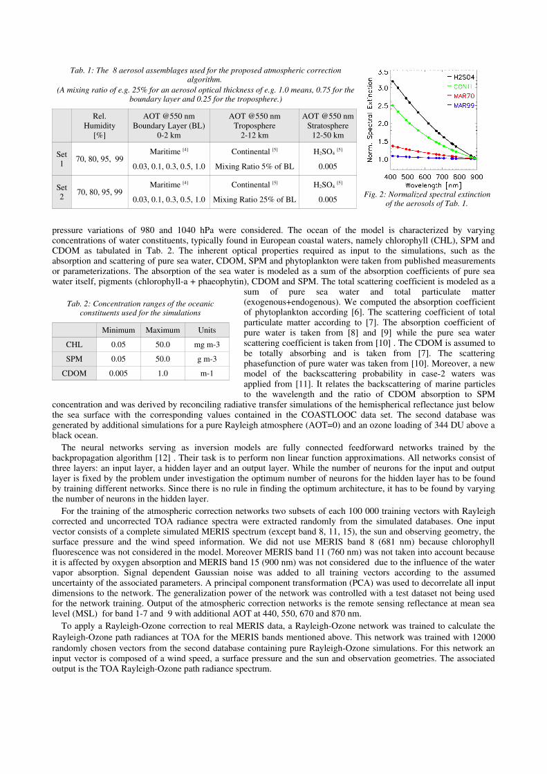
As forward model we used a radiative transfer code based on the matrix-operator method to generate two largedatabases which are used as data pools for the neural network training [2],[3]. The first database was generated withazimuthally resolved upward radiances in the MERIS channels just above the sea surface and at TOA for a variety ofsun and observing geometries. All simulations are based on a U.S. Standard atmosphere with a constant ozone loadingof 344 DU and were performed for a mixture of maritime [4], continental [5] and H2SO4 [5] aerosol types as outlined inTab. 1. As shown from the normalized spectral extinction coefficients of Fig. 1 no absorbing aerosols were taken intoaccount. The optical properties of these aerosols used as input for the radiative transfer simulations were derived priorfrom Mie calculations. Moreover, a rough sea surface characterized by wind speeds of 1.5 and 7.2 m/s and surface air___________________________________________

* Presented at the MERIS User Workshop, ESA ESRIN, Frascati, Italy, 10.-13. November 2003.

pressure variations of 980 and 1040 hPa were considered. The ocean of the model is characterized by varyingconcentrations of water constituents, typically found in European coastal waters, namely chlorophyll (CHL), SPM andCDOM as tabulated in Tab. 2. The inherent optical properties required as input to the simulations, such as theabsorption and scattering of pure sea water, CDOM, SPM and phytoplankton were taken from published measurementsor parameterizations. The absorption of the sea water is modeled as a sum of the absorption coefficients of pure seawater itself, pigments (chlorophyll-a + phaeophytin), CDOM and SPM. The total scattering coefficient is modeled as a

sum of pure sea water and total particulate matter(exogenous+endogenous). We computed the absorption coefficientof phytoplankton according [6]. The scattering coefficient of totalparticulate matter according to [7]. The absorption coefficient ofpure water is taken from [8] and [9] while the pure sea waterscattering coefficient is taken from [10] . The CDOM is assumed tobe totally absorbing and is taken from [7]. The scatteringphasefunction of pure water was taken from [10]. Moreover, a newmodel of the backscattering probability in case-2 waters wasapplied from [11]. It relates the backscattering of marine particlesto the wavelength and the ratio of CDOM absorption to SPM

concentration and was derived by reconciling radiative transfer simulations of the hemispherical reflectance just belowthe sea surface with the corresponding values contained in the COASTLOOC data set. The second database wasgenerated by additional simulations for a pure Rayleigh atmosphere (AOT=0) and an ozone loading of 344 DU above ablack ocean.

The neural networks serving as inversion models are fully connected feedforward networks trained by thebackpropagation algorithm [12] . Their task is to perform non linear function approximations. All networks consist ofthree layers: an input layer, a hidden layer and an output layer. While the number of neurons for the input and outputlayer is fixed by the problem under investigation the optimum number of neurons for the hidden layer has to be foundby training different networks. Since there is no rule in finding the optimum architecture, it has to be found by varyingthe number of neurons in the hidden layer.

For the training of the atmospheric correction networks two subsets of each 100 000 training vectors with Rayleighcorrected and uncorrected TOA radiance spectra were extracted randomly from the simulated databases. One inputvector consists of a complete simulated MERIS spectrum (except band 8, 11, 15), the sun and observing geometry, thesurface pressure and the wind speed information. We did not use MERIS band 8 (681 nm) because chlorophyllfluorescence was not considered in the model. Moreover MERIS band 11 (760 nm) was not taken into account becauseit is affected by oxygen absorption and MERIS band 15 (900 nm) was not considered due to the influence of the watervapor absorption. Signal dependent Gaussian noise was added to all training vectors according to the assumeduncertainty of the associated parameters. A principal component transformation (PCA) was used to decorrelate all inputdimensions to the network. The generalization power of the network was controlled with a test dataset not being usedfor the network training. Output of the atmospheric correction networks is the remote sensing reflectance at mean sealevel (MSL) for band 1-7 and 9 with additional AOT at 440, 550, 670 and 870 nm.

To apply a Rayleigh-Ozone correction to real MERIS data, a Rayleigh-Ozone network was trained to calculate theRayleigh-Ozone path radiances at TOA for the MERIS bands mentioned above. This network was trained with 12�000randomly chosen vectors from the second database containing pure Rayleigh-Ozone simulations. For this network aninput vector is composed of a wind speed, a surface pressure and the sun and observation geometries. The associatedoutput is the TOA Rayleigh-Ozone path radiance spectrum.

Tab. 1: The 8 aerosol assemblages used for the proposed atmospheric correctionalgorithm.

(A mixing ratio of e.g. 25% for an aerosol optical thickness of e.g. 1.0 means, 0.75 for theboundary layer and 0.25 for the troposphere.)

Rel.Humidity

[%]

AOT @550 nmBoundary Layer (BL)

0-2 km

AOT @550 nmTroposphere

2-12 km

AOT @550 nmStratosphere

12-50 km

Set1 70, 80, 95, 99

Maritime [4]

0.03, 0.1, 0.3, 0.5, 1.0

Continental [5]

Mixing Ratio 5% of BL

H2SO4 [5]

0.005

Set2 70, 80, 95, 99

Maritime [4]

0.03, 0.1, 0.3, 0.5, 1.0

Continental [5]

Mixing Ratio 25% of BL

H2SO4 [5]

0.005

Tab. 2: Concentration ranges of the oceanicconstituents used for the simulations

Minimum Maximum Units

CHL 0.05 50.0 mg m-3

SPM 0.05 50.0 g m-3

CDOM 0.005 1.0 m-1

Fig. 2: Normalized spectral extinctionof the aerosols of Tab. 1.

2.2. Data processing

When introducing real MERIS data to the networks two normalizations have to be applied to be consistent with thesimulation world. First the TOA radiances need to be normalized to the actual spectral solar constant values containedin the Level 1b data file. Second the TOA radiances have to be normalized to an ozone loading of 344 DU used in theradiative transfer simulations. Therefore the direct ozone transmission for the simulation with 344 DU and for theozone amount at the time of the MERIS overpath have to be calculated. The total ozone amount at the time of theMERIS measurement is taken from the resampled ECMWF data of the annotation dataset while the spectral ozoneextinction coefficients are taken from [13].

When applying a Rayleigh correction to the MERIS measurements first, the atmospheric correction is performed bytwo consecutive networks. First the Rayleigh-Ozone network calculates the TOA Rayleigh-Ozone path radiances forthe actual pressure and an ozone loading of 344 DU for each pixel. This output is used to correct the normalized TOAradiance spectra for Rayleigh scattering and ozone absorption and is then processed by the atmospheric correctionnetwork. If no Rayleigh-Ozone correction is applied to the TOA radiances only one network will do the atmosphericcorrection. Output of both networks consist of the remote sensing reflectances at mean sea level for 8 bands and theAOT at 4 wavelengths.

3 RESULTS AND VALIDATION

Validation of atmospheric correction algorithms are performed with the help ofcoincident in situ measurements of the marine reflectance and the spectral aerosoloptical thickness. Due to the lack marine reflectance measurements a validation of theproposed algorithm is achieved solely with the help of coincident CIMELsunphotometer measurements of the Aerosol Robotic Network (AERONET) [14] fromthe Helgoland Island (Fig. 2). Helgoland Island is located at 7.89°E longitude and 54.18°N latitude about 70 km off mainland in the German Bight. In the frame of this work 8MERIS tracks from the years 2002 and 2003 were processed with the outlined neuralnetwork atmospheric correction algorithms. From a 20 x 20 pixel box centered atHelgoland Island the median values of the retrieved neural network AOTs for aninversion with Rayleigh correction are compared with the median values of the sunphotometer measurements of a 2hour time window (Fig. 3). MERIS overpath time for the selected tracks is calculated to be between 10 and 10:30 UTC.

29.07.02 14.08.02 13.04.03 17.04.03

23.04.03 29.04.03 26.06.03 14.07.03

Fig. 3: Median of the neural network retrieved aerosol optical thickness (black) compared with the median of in situ sunphotometermeasurements from Helgoland Island (red). Black error bars represent the standard deviation for a 20x20 Pixel box. Red error bars

represent the standard deviation for the 2 hour time window of the in situ measurements.

Fig. 2: Helgoland Island

Therefore the time window for the AERONET data was selected between 9 and 11 UTC. Land pixels were rejectedwith the help of the Level 1b data flags. Moreover we applied an own cloud mask based on simple thresholds, sufficient

enough for ocean color purpose.For better intercomparison of all 8days the median AERONETvalues were interpolated on 550nm and scatter plotted versus theneural network results (Fig. 4).For AOTs less than 0.2 thenetwork retrieved AOTs showbetter results for an inversion withRayleigh and ozone correction.The overall RMSE for theRayleigh and ozone correctedinversion is with 0.05 lowercompared to the uncorrected with0.073 RMSE. Fig. 4 suggestsbetter performance for theRayleigh and ozone correctednetwork, but if one compares theresults for the derived AOT fieldsat 440 nm shown in Fig. 5, the

Rayleigh-Ozone network produces artificial patches in the lower left of the image which can be seen in the RGBcomposite as structures from the water and not from the atmosphere. Therefore it is helpful for the validation of theAOT not only to look at RMSE values but also at the derived structures of the AOT fields. Even though the Rayleighand ozone uncorrected network has a higher overall RMSE, it is leading to more reliable AOT structures. Along thecoastlines both networks achieved good results, which means that the retrieved AOTs are not influenced by sediments.

Due to the lack of in situ data the network derived remote sensing reflectances could not be validated. But samplespectra taken at 4 locations marked in Fig. 6 look reliable when comparing them with spectra taken from literature [15].The spectra of location 1 and 3 are typical for waters with moderate chlorophyll and sediment concentrations. While thespectra of location 2 and 4 are typical for moderate sediment and gelbstoff concentrations with some phytoplankton.Moreover the structures of the reflectances at 442.5 nm and 560.0 nm of Fig. 6 look feasible. Along the coastline thereflectance at 560.0 have higher values compared with 442.5 nm due to the sediments and the gelbstoff. In general, thecorrelation between the path reflectance and derived remote sensing reflectance at MSL should be low after appylingthe atmospheric correction. The correlation analysis of both reflectances for the West-to-East transact of Fig. 8 yields alow correlation of r=-0.299 at 442.5 nm and a higher correlation of r=-0.839 at 560.0 nm. The path reflectances werecalculated with an approximation of the diffuse transmittance given by [16].

Fig, 4: Scatter plots of the neural network retrieved median AOTs versus the median of thein situ measured AOTs from AERONET station Helgoland Island. With prior Rayleigh andozone correction (left). Without Rayleigh and ozone correction (right). Error bars represent

the standard deviation of the 20x20 pixel box and the 2h time window.

RGB composite AOT 440 Rayleigh+O3 corrected AOT 440

0.0 0.2 0.4 0.6 0.8 1.0

Fig. 5: RGB composite covering the German Bight as measured by MERIS on April 13th 2003 (left) with the associated neuralnetwork derived AOT field at 440 nm with Rayleigh and ozone correction (center) and without prior correction (right).

4 CONCLUSION

We proposed an atmospheric correction scheme forMERIS data above case-2 waters based on artificialneural networks and applied the algorithm to 8 MERISLevel 1b data tracks covering the German Bight. Thefast and robust inversion algorithm derives the remotesensing reflectance at mean sea level and the aerosoloptical thickness at 4 wavelengths. An overall RMSE of0.05 between 440 nm and 870 nm could be derived incomparing the spectral AOTs of an atmosphericcorrection network with prior Rayleigh and ozonecorrection with in situ AERONET data from HelgolandIsland. A slightly higher overall RMSE of 0.073 wasachieved by a network without Rayleigh and ozonecorrection. Although this network is less accurate, abetter separation of atmospheric and oceanic structurescould be obtained from this network. Further validation data are needed to analyze the differences between the networkcomputed spectral AOTs and AERONET. Other aerosol models like the suggested blue aerosol model may help toimprove the AOT retrieval at shorter wavelenghts. For the future in situ measurements of the marine reflectance likefrom SIMBADA are needed for validation of the neural network remote sensing reflectance.

RGB composite Remote sensing reflectance 442.5 nm Remote sensing reflectance 560.0 nm

0.001 [sr -1] 0.01Fig. 6: RGB composite covering the German Bight as measured by MERIS on April 13th 2003 (left) with labeled locations and atransact for analysis of the derived remote sensing reflectance at 442.5 nm (center) and 560.0 nm (right). Details Fig. 7 and 8.

[W-E] [W-E]

Fig. 8: TOA remote sensing reflectance RSTOA and the associatedneural network derived remote sensing reflectance at mean sea

level RSMSL for the transact of Fig. 6 from West to East. Pathreflectance RSPATH calculated with an approximation of the diffuse

transmittance td given by [16] according to [RSTOA-(td*RSMSL)].

[1] [2] [3] [4]

Fig. 7: TOA remote sensing reflectance spectra RSTOA and the associated neural network derived remote sensing reflectance spectraRSMSL at the 4 locations of Fig. 6.

5 ACKNOWLEDGEMENTS

This work was funded by the European Commission under the contract number EVG1 CT-2000-00034 (NAOC, NeuralNetwork Algorithms for Ocean Color). Moreover we thank the Roland Doerffer for his effort in establishing and maintaining the Helgoland Island AERONETstation.

6 REFERENCES

1. Morel M., and Prieur L., Analysis of Variations in Ocean Color, Limnology and Oceanography, 22(4), pp. 709 ff.,1977.

2. Fischer J., and Grassl H., Radiative transfer in an atmosphere-ocean system: an azimuthally dependent matrix-operator approach, Applied Optics , 23, 1032-1039, 1984.

3. Fell F., and Fischer J., Numerical simulation of the light field in the atmosphere-ocean system using the matrix-operator method, Journal of Quantitative Spectroscopy & Radiative Transfer, 69, 351-388, 2001.

4. Shettle E. P. And Fenn R. W., Models for the aerosols of the lower atmosphere and the effects of humidity variationson their optical properties, Environmental Research Papers, AFGL TR 79 0214, AFGL, 1979.

5. WCRP; World Climate Research Program, A preliminary cloudless standard atmosphere for radiation computation,Int. Ass. For Meteor. and Atm. Phys., Radiation Commission, WCP 112, 1986.

6. Bricaud A., Morel A., Babin M., Allali K. and Claustre H., Variations of light absorption by suspended particles withchlorophyll a concentration in oceanic (case 1) waters: Analysis and implications for bio optical models, Journalof Geophysical Research, 103, pp. 31033 31044, 1998.

7. Babin, M., Coastal surveillance through observation of ocean colour (COASTLOOC), Final Report, Project ENV4-CT96-0310, 233 pp., Laboratoire de Physique et Chimie Marines, Villefranche-sur-mer, France, 2000.

8. Pope R., and Fry E. S., Absorption spectrum (380 700 nm) of pure water. II. Integrating cavity measurements,Applied Optics, 36, pp. 8710 8723, 1997.

9. Hale G. M. and Querry M. R., Optical constants of water in the 200 nm to 200 mm wavelength region, AppliedOptics, 12, pp. 555 563, 1973.

10. Morel A., Optical properties of pure water and sea water. In: Optical Aspects of Oceanography, Edited by Jerlovand Steemann Nielsen, Academic, pp. 1 24, 1974.

11. Zhang T., Fell F. and Fischer J., Modeling the backscattering ratio of marine particles in case II waters,Proceedings of Ocean Optics XVI, published on CD-ROM, Santa Fe, New Mexico, USA, 2002.

12. Rummelhart D. and McClelland J., Parallel Distributed Processing, MIT Press, Cambridge, Massachusetts, 1986.

13. Baur, F. (Editor), Linkes Meteorologisches Taschenbuch, Band 2, Leipzig: Akademische Verlagsgesellschaft Geest& Porting, 1953.

14. http://aeronet.gsfc.nasa.gov/

15. IOCCG, Reports of the International Ocean-Colour Coordinating Group, IOCCG Report No. 3, Remote Sensing ofOcean Colour in Coastal, and Other Optically-Complex, Waters, Ed. by Shubha Sathyendranath, 2000.

16. Gordon H. R., Atmospheric correction of ocean color imagery in the Earth Observing Sytem era, Journal ofGeophysical Research, Vol. 102, NO. D14, at page 17099, 1997.