atmospheric correction of hj-1 ccd imagery over turbid ... · atmospheric correction of hj-1 ccd...

Atmospheric correction of HJ-1 CCD imagery over turbid lake waters

Minwei Zhang,1 Junwu Tang,2 Qing Dong,1,* Hongtao Duan,3 and Qian Shen1 1Key Laboratory of Digital Earth Science, Institute of Remote Sensing and Digital Earth, Chinese Academy of

Sciences, Beijing 100094, China 2National Ocean Technology Center, Tianjin 300112, China

3Nanjing Institute of Geography and Limnology, Chinese Academy of Sciences, Nanjing, 210008, China *[email protected]

Abstract: We have presented an atmospheric correction algorithm for HJ-1 CCD imagery over Lakes Taihu and Chaohu with highly turbid waters. The Rayleigh scattering radiance (Lr) is calculated using the hyperspectral Lr with a wavelength interval 1nm. The hyperspectral Lr is interpolated from Lr in the central wavelengths of MODIS bands, which are converted from the band response-averaged Lr calculated using the Rayleigh look up tables (LUTs) in SeaDAS6.1. The scattering radiance due to aerosol (La) is interpolated from La at MODIS band 869nm, which is derived from MODIS imagery using a shortwave infrared atmospheric correction scheme. The accuracy of the atmospheric correction algorithm is firstly evaluated by comparing the CCD measured remote sensing reflectance (Rrs) with MODIS measurements, which are validated by the in situ data. The CCD measured Rrs is further validated by the in situ data for a total of 30 observation stations within ± 1h time window of satellite overpass and field measurements. The validation shows the mean relative errors about 0.341, 0.259, 0.293 and 0.803 at blue, green, red and near infrared bands.

©2014 Optical Society of America

OCIS codes: (010.1285) Atmospheric correction; (010.0010) Atmospheric and oceanic optics; (010.0280) Remote sensing and sensors.

References and links

1. Y. Li, Y. Xue, X. He, and J. Guang, “High-resolution aerosol remote sensing retrieval over urban areas by synergetic use of HJ-1 CCD and MODIS data,” Atmos. Environ. 46, 173–180 (2012).

2. H. R. Gordon and M. Wang, “Retrieval of water-leaving radiance and aerosol optical thickness over the oceans with SeaWiFS: a preliminary algorithm,” Appl. Opt. 33(3), 443–452 (1994).

3. A. Morel and L. Prieur, “Analysis of variations in ocean color,” Limnol. Oceanogr. 22(4), 709–722 (1977). 4. D. A. Siegel, M. Wang, S. Maritorena, and W. Robinson, “Atmospheric correction of satellite ocean color

imagery: the black pixel assumption,” Appl. Opt. 39(21), 3582–3591 (2000). 5. M. Wang and W. Shi, “Estimation of ocean contribution at the MODIS near-infrared wavelengths along the east

coast of the U.S.: Two case studies,” Geophys. Res. Lett. 32(13), L13606 (2005). 6. R. A. Arnone, M. Sydor, and R. W. Gould, Jr., “Remote sensing reflectance of case 2 waters,” Ocean Optics

XIII 2963, 222–227 (1996). 7. X. He and D. Pan, “A practical method of atmospheric correction of SeaWiFS imagery for turbid coastal and

inland waters,” Proc. SPIE 4892, 494–505 (2003). 8. S. J. Lavender, M. H. Pinkerton, G. F. Moore, J. Aiken, and D. Blondeau-Patissier, “Modification to the

atmospheric correction of SeaWiFS ocean color images over turbid waters,” Cont. Shelf Res. 25(4), 539–555 (2005).

9. J. Ding, J. Tang, Q. Song, and X. Wang, “Atmospheric correction for Chinese coastal turbid waters using iteration and optimization method,” J. Remote Sens. 10, 732–741 (2006).

10. C. Hu, K. L. Carder, and F. E. Muller-Karger, “Atmospheric correction of SeaWiFS imagery over turbid coastal waters: a practical method,” Remote Sens. Environ. 74(2), 195–206 (2000).

11. K. G. Ruddick, F. Ovidio, and M. Rijkeboer, “Atmospheric correction of SeaWiFS imagery for turbid coastal and inland waters,” Appl. Opt. 39(6), 897–912 (2000).

12. P. Dash, N. Walker, D. Mishra, E. d’Sa, and S. Ladner, “Atmospheric correction and vicarious calibration of Oceansat-1 Ocean Color Monitor(OCM) data in coastal case 2 waters,” Remote Sens. 4(12), 1716–1740 (2012).

13. M. Wang, “Remote sensing of the ocean contributions from ultraviolet to near-infrared using the shortwave infrared bands: simulations,” Appl. Opt. 46(9), 1535–1547 (2007).

#206330 - $15.00 USD Received 14 Feb 2014; revised 14 Mar 2014; accepted 14 Mar 2014; published 27 Mar 2014(C) 2014 OSA 7 April 2014 | Vol. 22, No. 7 | DOI:10.1364/OE.22.007906 | OPTICS EXPRESS 7906

14. M. Wang, W. Shi, and J. Tang, “Water property monitoring and assessment for China’s inland Lake Taihu from MODIS-Aqua measurements,” Remote Sens. Environ. 115(3), 841–854 (2011).

15. G. M. Hale and M. R. Querry, “Optical constants of water in the 200-nm to 200-micrometer wavelength region,” Appl. Opt. 12(3), 555–563 (1973).

16. L. Gross-Colzy, S. Colzy, R. Frouin, and P. Henry, “A general ocean color atmospheric correction scheme based on principal components analysis: Part I. performance on Case 1 and Case 2 waters,” Proc. SPIE 6680, 668002 (2007).

17. T. Schroeder, I. Behnert, M. Schaale, J. Fischer, and R. Doerffer, “Atmospheric correction algorithm for MERIS above case-2 waters,” Int. J. Remote Sens. 28(7), 1469–1486 (2007).

18. C. Hu, F. E. Muller-Karger, S. Andrefouet, and K. L. Carder, “Atmospheric correction and cross-calibration of LANDSAT-7/ETM+ imagery over aquatic environments: A multiplatform approach using SeaWiFS/MODIS,” Remote Sens. Environ. 78(1–2), 99–107 (2001).

19. J. Li, B. Zhang, Z. Chen, and Q. Shen, “Atmospheric correction of CBERS CCD images with MODIS data,” Sci. China Ser. E 49, 149–158 (2006).

20. J. Chen, J. Fu, and M. Zhang, “An atmospheric correction algorithm for Landsat/TM imagery basing on inverse distance spatial interpolation algorithm: a case study in Taihu Lake,” IEEE J. Sel. Top. Appl. Earth Observ. Remote Sens. 4(4), 882–889 (2011).

21. A. G. Dekker, R. J. Vos, and S. W. Peters, “Comparison of remote sensing data, model results and in situ data for total suspended matter (TSM) in the southern Frisian lakes,” Sci. Total Environ. 268(1–3), 197–214 (2001).

22. C. Hu, Z. Chen, T. D. Clayton, P. Swarzenski, J. C. Brock, and F. E. Muller-Karger, “Assessment of estuarine water-quality indicators using MODIS medium-resolution bands: initial results from Tampa Bay, Florida,” Remote Sens. Environ. 93(3), 423–441 (2004).

23. A. Morel, Y. Huot, B. Gentili, P. J. Werdell, S. B. Hooker, and B. A. Franz, “Examining the consistency of products derived from various ocean color sensors in open ocean (Case 1) waters in the perspective of a multi-sensor approach,” Remote Sens. Environ. 111(1), 69–88 (2007).

24. M. Zhang, J. Tang, Q. Dong, Q. Song, and J. Ding, “Retrieval of total suspended matter concentration in the Yellow and East China Seas from MODIS imagery,” Remote Sens. Environ. 114(2), 392–403 (2010).

25. J. Chen, W. Quan, G. Yao, and T. Cui, “Retrieval of absorption and backscattering coefficients from HJ-1A/CCD imagery in coastal waters,” Opt. Express 21(5), 5803–5821 (2013).

26. J. Chen and W. Quan, “An improved algorithm for retrieving chlorophyll-a from the Yellow River Estuary using MODIS Imagery,” Environ. Monit. Assess. 185(3), 2243–2255 (2013).

27. L. Guo, P. Xie, L. Ni, W. Hu, and H. Li, “The status of fishery resources of lake Chaohu and its response to eutrophication,” Acta Hydrobiol. Sin. 31, 700–705 (2007).

28. J. L. Mueller, C. Davis, R. Arnone, R. Frouin, K. L. Carder, Z. Lee, R. G. Steward, S. Hooker, C. D. Mobley, and S. McLean, “Above-water radiance and remote sensing reflectance measurements and analysis protocols,” in Radiometric Measurements and Data Analysis Protocols, Vol. III in Ocean Optics Protocols for Satellite Ocean Color Sensor Validation, revision 4, (2003), Chap. 3, pp. 21–30.

29. C. D. Mobley, “Estimation of the remote-sensing reflectance from above-surface measurements,” Appl. Opt. 38(36), 7442–7455 (1999).

30. R. Ma, J. Tang, J. Dai, Y. Zhang, and Q. Song, “Absorption and scattering properties of water body in Taihu Lake, China: absorption,” Int. J. Remote Sens. 27(19), 4277–4304 (2006).

31. M. Rijkeboer, A. G. Dekker, and H. J. Gons, “Subsurface irradiance reflectance spectra of inland waters differing in morphometry and hydrology,” Aquat. Ecol. 31(3), 313–323 (1998).

32. D. Gurlin, A. A. Gitelson, and W. J. Moses, “Remote estimation of chl-a concentration in turbid productive waters - Return to a simple two-band NIR-red model?” Remote Sens. Environ. 115(12), 3479–3490 (2011).

33. Y. Zhang, L. Feng, J. Li, L. Luo, Y. Yin, M. Liu, and Y. Li, “Seasonal–spatial variation and remote sensing of phytoplankton absorption in Lake Taihu, a large eutrophic and shallow lake in China,” J. Plankton Res. 32(7), 1023–1037 (2010).

34. C. C. Trees, R. R. Bidigare, D. M. Karl, L. V. Heukelem, and J. Dore, “Fluorometric chlorophyll a: sampling, laboratory methods, and data analysis protocols,” in Biogeochemical and Bio-optical Measurements and Data Analysis Protocols, Vol. V in Ocean Optics Protocols for Satellite Ocean Color Sensor Validation, revision 5 (2003), Chap. 3, pp. 15–25.

35. J. D. H. Strickland and T. R. Parsons, A Practical Handbook of Seawater Analysis, 2nd ed. (Board of Canada, 1972).

36. M. Wang, “The Rayleigh lookup tables for the SeaWiFS data processing: accounting for the effects of ocean surface roughness,” Int. J. Remote Sens. 23(13), 2693–2702 (2002).

37. M. Wang, “A refinement for the Rayleigh radiance computation with variation of the atmospheric pressure,” Int. J. Remote Sens. 26(24), 5651–5663 (2005).

38. C. Cox and W. Munk, “Measurement of the roughness of the sea surface from photographs of the sun’s glitter,” J. Opt. Soc. Am. 44(11), 838–850 (1954).

39. M. Wang and S. W. Bailey, “Correction of sun glint contamination on the SeaWiFS ocean and atmosphere products,” Appl. Opt. 40(27), 4790–4798 (2001).

40. H. R. Gordon and M. Wang, “Influence of oceanic whitecaps on atmospheric correction of ocean-color sensors,” Appl. Opt. 33(33), 7754–7763 (1994).

41. W. W. Gregg and K. L. Carder, “A simple spectral solar irradiance model for cloudless maritime atmospheres,” Limnol. Oceanogr. 35(8), 1657–1675 (1990).

42. R. E. Eplee, W. D. Robinson, S. W. Bailey, D. K. Clark, P. J. Werdell, M. Wang, R. A. Barnes, and C. R. McClain, “Calibration of SeaWiFS. II. vicarious techniques,” Appl. Opt. 40(36), 6701–6718 (2001).


43. H. R. Gordon and D. J. Castaño, “Aerosol analysis with the Coastal zone color scanner: A simple method for including multiple scattering effects,” Appl. Opt. 28(7), 1320–1326 (1989).

44. H. R. Gordon and D. J. Castaño, “Coastal zone color scanner atmospheric correction algorithm: multiple scattering effects,” Appl. Opt. 26(11), 2111–2122 (1987).

45. H. R. Gordon, “Remote sensing of ocean color: a methodology for dealing with broad spectral bands and significant out-of-band response,” Appl. Opt. 34(36), 8363–8374 (1995).

46. M. Zhang, R. Ma, J. Li, B. Zhang, and H. Duan, “A validation study of an improved SWIR iterative atmospheric correction algorithm for MODIS-Aqua measurements in Lake Taihu, China,” IEEE Trans. Geosci. Remote Sens. 52, 4686–4695 (2014).

47. M. Wang, S. Son, and W. Shi, “Evaluation of MODIS SWIR and NIR-SWIR atmospheric correction algorithms using SeaBASS data,” Remote Sens. Environ. 113(3), 635–644 (2009).

48. H. R. Gordon, D. K. Clark, J. W. Brown, O. B. Brown, R. H. Evans, and W. W. Broenkow, “Phytoplankton pigment concentrations in the Middle Atlantic Bight: comparison of ship determinations and CZCS estimates,” Appl. Opt. 22(1), 20–36 (1983).

49. S. W. Bailey and P. J. Werdell, “A multi-sensor approach for the on-orbit validation of ocean color satellite data products,” Remote Sens. Environ. 102(1–2), 12–23 (2006).

50. D. Wang, D. Morton, J. Masek, A. Wu, J. Nagol, X. Xiong, R. Levy, E. Vermote, and R. Wolfe, “Impact of sensor degradation on the MODIS NDVI time series,” Remote Sens. Environ. 119, 55–61 (2012).

51. R. Ma, H. Duan, X. Gu, and S. Zhang, “Detecting aquatic vegetation changes in Taihu Lake, China using multi-temporal satellite imagery,” Sensors 8(6), 3988–4005 (2008).

52. P. N. Reinersman and K. L. Carder, “Monte Carlo simulation of the atmospheric point-spread function with an application to correction for the adjacency effect,” Appl. Opt. 34(21), 4453–4471 (1995).

53. Q. Li, S. Niu, and D. Xu, “Remote sensing of aerosol optical properties and air pollution with MFRSR measurements in Taihu region,” T. Atmos. Sci. 35, 364–371 (2012).

54. L. Tian, J. Lu, X. Chen, Z. Yu, J. Xiao, F. Qiu, and X. Zhao, “Atmospheric correction of HJ-1A/B CCD images over Chinese coastal waters using MODIS-Terra aerosol data,” Sci. China Ser. E 53(S1), 191–195 (2010).

55. Z. Yu, X. Chen, L. Tian, and B. Zhou, “Atmospheric correction method for Poyang lake HJ-1A/B CCD image,” Geomatics Info. Sci. Wuhan U. 37, 1078–1082 (2012).

56. R. L. Miller and B. A. McKee, “Using MODIS Terra 250 m imagery to map concentrations of total suspended matter in coastal waters,” Remote Sens. Environ. 93(1–2), 259–266 (2004).

57. V. Rodríguez-Guzmán and F. Gilbes-Santaella, “Using MODIS 250 m imagery to estimate total suspended sediment in a tropical open bay,” Int. J. Syst. Appl. Eng. Dev. 3, 36–44 (2009).

58. B. Nechad, K. Ruddick, and Y. Park, “Calibration and validation of a generic multisensor algorithm for mapping of total suspended matter in turbid waters,” Remote Sens. Environ. 114(4), 854–866 (2010).

59. G. Neukermans, K. Ruddick, E. Bernard, D. Ramon, B. Nechad, and P. Y. Deschamps, “Mapping total suspended matter from geostationary satellites: a feasibility study with SEVIRI in the Southern North Sea,” Opt. Express 17(16), 14029–14052 (2009).

60. Z. Chen, C. Hu, and F. Muller-Karger, “Monitoring turbidity in Tampa bay using MODIS/Aqua 250 m imagery,” Remote Sens. Environ. 109(2), 207–220 (2007).

61. G. Dall’Olmo and A. A. Gitelson, “Effect of bio-optical parameter variability on the remote estimation of chlorophyll-a concentration in turbid productive waters: experimental results,” Appl. Opt. 44(3), 412–422 (2005).

62. G. Zhou, Q. Liu, R. Ma, and G. Tian, “Inversion of chlorophyll-a concentration in turbid water of lake Taihu based on optimized multi-spectral combination,” J. Lake Sci. 20, 153–159 (2008).

63. C. Le, Y. Li, Y. Zha, D. Sun, C. Huang, and H. Lu, “A four-band semi-analytical model for estimation chlorophyll a in highly turbid lakes: the case of Taihu Lake, China,” Remote Sens. Environ. 113(6), 1175–1182 (2009).

64. Z. Lee, M. Darecki, K. L. Carder, C. Davis, D. Stramski, and W. J. Rhea, “Diffuse attenuation coefficient of downwelling irradiance: An evaluation of remote sensing methods,” J. Geophys. Res. 110, C02017 (2005).

65. X. A. Xia, H. B. Chen, and P. C. Wang, “Validation of MODIS aerosol retrievals and evaluation of potential cloud contamination in east Asia,” J. Environ. Sci. China 16(5), 832–837 (2004).

1. Introduction

The satellite constellation including HJ-1A and HJ-1B, launched on Sep. 6, 2008, is designed for monitoring the environment and forecasting the disaster [1]. Two charge-coupled device(CCD) cameras (named CCD1 and CCD2) aboard each satellite, with a spatial resolution about 30m and four bands including blue, green, red, and near infrared (NIR) ones, have the potential of monitoring the color of inland waters with high spatial variation of optical properties.

Due to the complexity of water optical properties, atmospheric correction (AC) is still a challenge for the application of satellite remote sensing in monitoring the color of inland waters. The standard AC algorithm for case 1 waters [2] fails when applied to inland area, which show characteristics of case 2 waters (the definitions of case 1 and 2 waters were described by [3]). The failure results from invalid assumption of black water at NIR bands


[4,5]. Many algorithms have been developed for the atmospheric correction of case 2 waters using data not only from ocean color sensors (such as SeaWiFS, MODIS and MERIS) but also from sensors primarily developed for monitoring land targets (such as TM). The algorithms for ocean color sensors can be classified into three categories. The first one is the iterative algorithms [6–9], where the spectral relationship is used to calculate the NIR contribution in order to use the AC algorithm based on the black water assumption. The second one is based on the assumption of low variation of aerosol [10–12]. The third one is the shortwave infrared (SWIR) scheme [13,14] with black water assumption in SWIR wavelengths [15]. Other AC algorithms are developed by means of a multi-parameter inversion using the complete spectral information at visible to NIR bands and coupled atmospheric and oceanic radiative transfer model. The inversion is based on principle components analysis (PCA) [16] or neural networks (NN) [17] techniques. The AC algorithms for data from sensors like TM are developed using the aerosol information either provided by ocean color sensors [18, 19] or in situ data [20] to calculate the aerosol scattering radiance.

Satellite remote sensing has been used to monitor the water quality in oceanic and coastal regions [21–26]. However, the algorithms developed for oceanic and coastal waters fail when applied to lake waters due to the complicated optical properties, which result from the combined effects of shallow water and sediment resuspension. On the other hand, the AC algorithms described above cannot be applied to CCD (CCD means both CCD1 and CCD2 aboard HJ-1A and HJ-1B) due to the difference of band specifications. An AC algorithm is in need for CCD imagery when applied to quantitatively monitor the optical properties of lake waters. It is challenged to develop the AC algorithms for CCD over lake waters, primarily due to the poorly documented optical properties of fresh waters and the optical path variation resulted from the lake altitudes. The challenge is also due to the adjacency effects and spatial resolution. The latter is addressed in this study. CCD doesn’t meet the minimum requirement for the atmospheric correction with at least two NIR or SWIR bands. As a result, other data have to be used in developing the AC algorithm.

The overall aim of this paper is to develop an AC algorithm for CCD imagery over turbid lake waters. The accuracy of the algorithm is firstly evaluated by comparing with MODIS measured spectra, which are validated using in situ data. The algorithm is further validated by in situ data. Using the CCD measured Rrs, the development of an algal bloom occurred in Lake Taihu is monitored. The potential application in quantifying the concentration of water’s component and the limitations of the algorithm are discussed.

2. Data

2.1. Study area

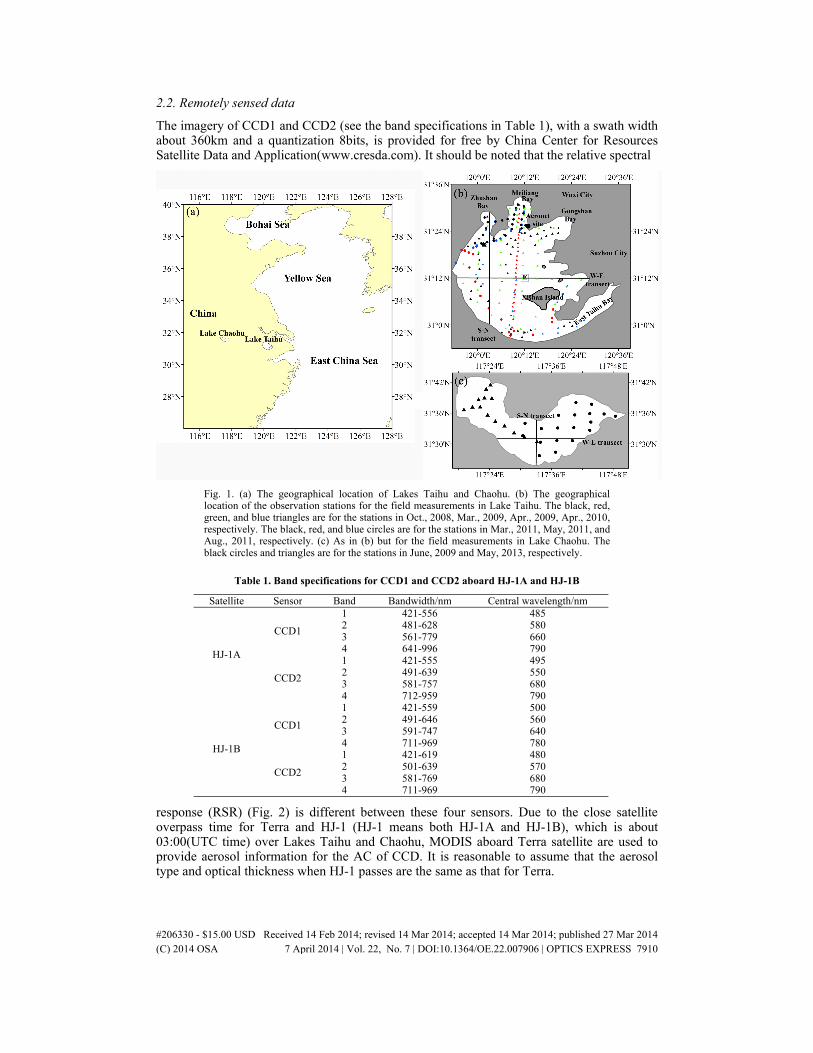
Lake Taihu with an area about 2338km2 (see the geographical location in Fig. 1(a)) is the third largest freshwater lake in China. The water in the lake is polluted by nutrient-laden river runoff and algal bloom is frequently occurred, affecting the water usage of nearby residents. As a result, there is an urgent need for monitoring the water quality and understanding the biological, optical, and ecological process in the lake.

Lake Chaohu well known for fishery is one of the five freshwater lakes in China, with an area about 775km2. The lake is semi-enclosed since a floodgate was built in the southwest exit in 1962. Water quality is deteriorating primarily due to the terrestrial inputs and also due to the decrease of self-purification resulted from the construction of the floodgate. The fish species have decreased 40% since 1980s due to the pollution [27]. The water quality monitoring is in need for promoting the fishery development and for the water usage in daily life for nearby residents.


2.2. Remotely sensed data

The imagery of CCD1 and CCD2 (see the band specifications in Table 1), with a swath width about 360km and a quantization 8bits, is provided for free by China Center for Resources Satellite Data and Application(www.cresda.com). It should be noted that the relative spectral

Fig. 1. (a) The geographical location of Lakes Taihu and Chaohu. (b) The geographical location of the observation stations for the field measurements in Lake Taihu. The black, red, green, and blue triangles are for the stations in Oct., 2008, Mar., 2009, Apr., 2009, Apr., 2010, respectively. The black, red, and blue circles are for the stations in Mar., 2011, May, 2011, and Aug., 2011, respectively. (c) As in (b) but for the field measurements in Lake Chaohu. The black circles and triangles are for the stations in June, 2009 and May, 2013, respectively.

Table 1. Band specifications for CCD1 and CCD2 aboard HJ-1A and HJ-1B

Satellite Sensor Band Bandwidth/nm Central wavelength/nm

HJ-1A

CCD1

1 421-556 4852 481-628 5803 561-779 6604 641-996 790

CCD2

1 421-555 4952 491-639 5503 581-757 6804 712-959 790

HJ-1B

CCD1

1 421-559 5002 491-646 5603 591-747 6404 711-969 780

CCD2

1 421-619 4802 501-639 5703 581-769 6804 711-969 790

response (RSR) (Fig. 2) is different between these four sensors. Due to the close satellite overpass time for Terra and HJ-1 (HJ-1 means both HJ-1A and HJ-1B), which is about 03:00(UTC time) over Lakes Taihu and Chaohu, MODIS aboard Terra satellite are used to provide aerosol information for the AC of CCD. It is reasonable to assume that the aerosol type and optical thickness when HJ-1 passes are the same as that for Terra.


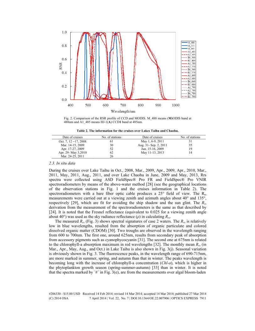
Fig. 2. Comparison of the RSR profile of CCD and MODIS. M_488 means (M)ODIS band at 488nm and A1_485 means HJ-1(A) CCD1 band at 485nm.

Table 2. The information for the cruises over Lakes Taihu and Chaohu.

Date of cruises No. of stations Date of cruises No. of stations Oct. 7, 12 −17, 2008 61 May 1, 6-9, 2011 31

Mar. 14-15, 2009 30 Aug. 31- Sep. 2, 2011 35 Apr. 17-27, 2009 52 Jun. 15-16, 2009 19

Apr. 29- May 3,2010 62 May 11-13, 2013 14 Mar. 24-25, 2011 26

2.3. In situ data

During the cruises over Lake Taihu in Oct., 2008, Mar., 2009, Apr., 2009, Apr., 2010, Mar., 2011, May, 2011, Aug., 2011, and over Lake Chaohu in June, 2009 and May, 2013, Rrs spectra were collected using ASD FieldSpec® Pro FR and FieldSpec® Pro VNIR spectroradiometers by means of the above-water method [28] (see the geographical locations of the observation stations in Fig. 1 and the cruises information in Table 2). The spectroradiometers with a bare fiber optic cable produces a 25° field of view. The Rrs measurements were carried out at a viewing zenith and azimuth angles about 40° and 135°, respectively [29], which are fit for avoiding the ship shadow and the sun glint. The Rrs derivation from the measurement of the spectroradiometers is the same as that described by [24]. It is noted that the Fresnel reflectance (equivalent to 0.025 for a viewing zenith angle about 40°) was used as the sky radiance reflectance (ρ) in calculating Rrs.

The measured Rrs (Fig. 3) shows spectral signatures of case 2 waters. The Rrs is relatively low in blue wavelengths, resulted from the absorption of organic particulate and colored dissolved organic matter (CDOM) [30]. Two troughs are observed in the wavelength ranging from 600 to 700nm. The first one, around 625nm, results from secondary peak of absorption from accessory pigments such as cyanophycocyanin [31]. The second one at 675nm is related to the chlorophyll-a absorption maximum in red wavelengths [32]. The monthly mean Rrs (in Mar., Apr., May, Aug., and Oct.) in Lake Taihu is also shown in Fig. 3(j). Seasonal variation is obviously shown in Fig. 3. The fluorescence peaks, in the wavelength range of 690-715nm, are more marked in summer, spring, and autumn than that in winter. The peaks wavelength is becoming long with the increase of chlorophyll-a concentration (Chl-a), which is higher in the phytoplankton growth season (spring-summer-autumn) [33] than in winter. It is noted that the spectra marked by ´#´ in Fig. 3(e), are from the measurements over algal bloom-laden


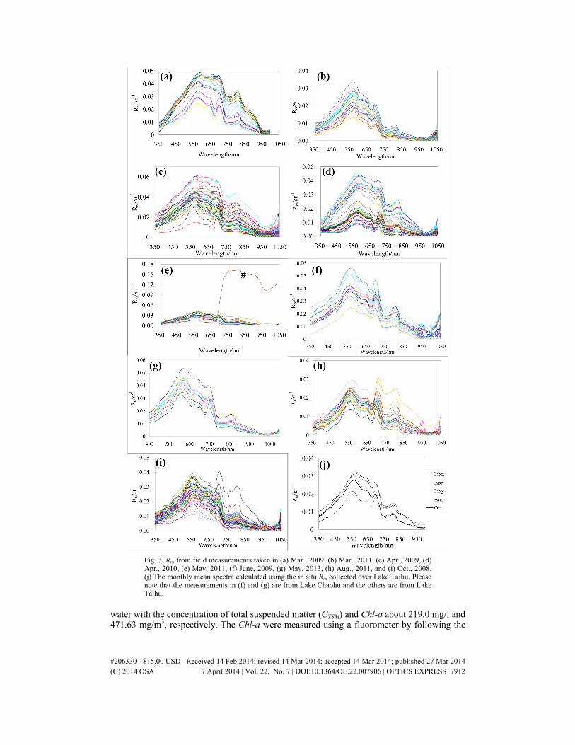
Fig. 3. Rrs from field measurements taken in (a) Mar., 2009, (b) Mar., 2011, (c) Apr., 2009, (d) Apr., 2010, (e) May, 2011, (f) June, 2009, (g) May, 2013, (h) Aug., 2011, and (i) Oct., 2008. (j) The monthly mean spectra calculated using the in situ Rrs collected over Lake Taihu. Please note that the measurements in (f) and (g) are from Lake Chaohu and the others are from Lake Taihu.

water with the concentration of total suspended matter (CTSM) and Chl-a about 219.0 mg/l and 471.63 mg/m3, respectively. The Chl-a were measured using a fluorometer by following the


protocol described by [34] and the CTSM were measured by means of the weighing method described by [35].

3. Atmospheric correction of CCD imagery

Scattering radiance due to air molecule (Lr) and aerosol (La) account for over 90% of the top-of-atmosphere (TOA) radiance (Lt) received by a remote sensor in the visible wavelengths [36]. Lw is less than 10%. As a result, the atmospheric correction, which removes atmospheric path radiance from Lt, is a key procedure in quantitative remote sensing of water color. Lt in the wavelength λ is given by Eq. (1) [2]:

t r a g w( ) ( ) ( ) ( ) ( ) ( ) ( ) ( ) ( )fL L L T L t L t Lλ λ λ λ λ λ λ λ λ= + + + + (1)

Lg is the direct sun glint. Lf is the scattering radiance due to whitecaps. T and t are direct and diffuse transmittance at sensor viewing direction. Lr can be calculated with an uncertainty within 0.1% in blue wavelengths and within 0.05% in green to NIR wavelengths [37]. For the calculation of Lg, sun glint coefficient is derived using the model proposed by [38]. Lg can be neglected if the coefficient is smaller than the threshold (0.0001 in this study). Otherwise, Lg is calculated by means of the method presented by [39]. Lf is calculated using the method developed by [40]. The scattering reflectance ρr, ρa, ρg, ρf, and ρw are given by

0 s/ (F cos )x xLρ π θ= (2)

where x means r, a, g, f, and w. F0 is the instantaneous extraterrestrial solar irradiance F´ reduced by two trips through the ozone layer, i. e.,

0 oz vF F exp[ (1/ cos 1/ cos )]sτ θ θ′= − + (3)

θv is the zenith angle of a vector from the pixel to the sensor and θs is the sun zenith angle. τoz is the ozone optical thickness given by

oz oz oz( ) ( )k Uτ λ λ= (4)

The specific absorption coefficients koz are presented by [41] and the ozone contents Uoz are from http://oceandata.sci.gsfc.nasa.gov/Ancillary/Meterological.

3.1. Rayleigh scattering

The scattering radiance due to air molecule (named Rayleigh scattering) of CCD is converted from the Rayleigh scattering radiance at MODIS bands, which are calculated using the Rayleigh lookup tables (LUTs). The dependency in λ−4 is used in the conversion [18]. The conversion factor β, from response-averaged Rayleigh optical thickness to that in the central wavelength is given by Eq. (5):

MOD0( )/ ( )r rβ τ λ τ λ= < > (5)

τr(λ0) is Rayleigh optical thickness in the central wavelength λ0 of MODIS band. <τr (λ)>MOD

is the response-averaged Rayleigh optical thickness at MODIS band, calculated by Eq. (6).

( ) ( ) ( ) ( ) ( ) ( )0 0/MODr r S F d S F dτ λ τ λ λ λ λ λ λ λ< > = (6)

S(λ) is the RSR of MODIS bands [42]. Using Eqs. (5)–(7), β are estimated as 1.0278, 0.9973, 0.9755, 0.9963, 0.9968, 1.0041, 0.994, 1.0013, 0.9999, 1.0028, 0.9806, 0.9911, and 0.9904 for MODIS bands at 412, 443, 469, 488, 531, 547, 555, 645, 667, 678, 748, 859, and 869 nm, respectively.

4 2 4( ) 0.008569 (1 0.0113 0.00013 ) in µmrτ λ λ λ λ λ− − −= + + (7)


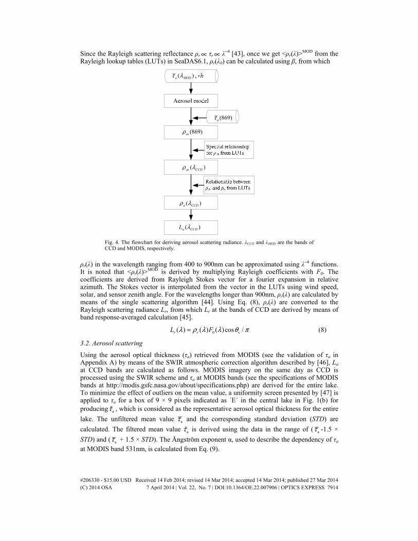
Since the Rayleigh scattering reflectance ρr ∝ τr ∝ λ−4 [43], once we get <ρr(λ)>MOD from the

Rayleigh lookup tables (LUTs) in SeaDAS6.1, ρr(λ0) can be calculated using β, from which

)869(~aτ

)(~MODa λτ

)869(asρ

)( CCDas λρ

)( CCDa λρ

)( CCDaL λ

Fig. 4. The flowchart for deriving aerosol scattering radiance. λCCD and λMOD are the bands of CCD and MODIS, respectively.

ρr(λ) in the wavelength ranging from 400 to 900nm can be approximated using λ−4 functions. It is noted that <ρr(λ)>

MOD is derived by multiplying Rayleigh coefficients with F0. The coefficients are derived from Rayleigh Stokes vector for a fourier expansion in relative azimuth. The Stokes vector is interpolated from the vector in the LUTs using wind speed, solar, and sensor zenith angle. For the wavelengths longer than 900nm, ρr(λ) are calculated by means of the single scattering algorithm [44]. Using Eq. (8), ρr(λ) are converted to the Rayleigh scattering radiance Lr, from which Lr at the bands of CCD are derived by means of band response-averaged calculation [45].

0 s( ) ( ) ( )cos /r rL Fλ ρ λ λ θ π= (8)

3.2. Aerosol scattering

Using the aerosol optical thickness (τa) retrieved from MODIS (see the validation of τa in Appendix A) by means of the SWIR atmospheric correction algorithm described by [46], La at CCD bands are calculated as follows. MODIS imagery on the same day as CCD is processed using the SWIR scheme and τa at MODIS bands (see the specifications of MODIS bands at http://modis.gsfc.nasa.gov/about/specifications.php) are derived for the entire lake. To minimize the effect of outliers on the mean value, a uniformity screen presented by [47] is applied to τa for a box of 9 × 9 pixels indicated as ´E´ in the central lake in Fig. 1(b) for producing aτ , which is considered as the representative aerosol optical thickness for the entire

lake. The unfiltered mean value aτ and the corresponding standard deviation (STD) are

calculated. The filtered mean value aτ is derived using the data in the range of ( aτ -1.5 ×

STD) and ( aτ + 1.5 × STD). The Ångström exponent α, used to describe the dependency of τa at MODIS band 531nm, is calculated from Eq. (9).


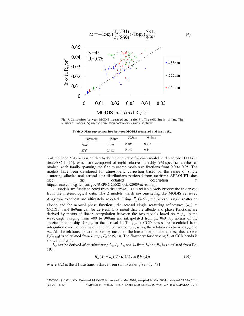
(531) 531( ) / ( )

869(869)log loga

e ea

ττα = − (9)

Fig. 5. Comparison between MODIS measured and in situ Rrs. The solid line is 1:1 line. The number of stations (N) and the correlation coefficient(R) are also shown.

Table 3. Matchup comparison between MODIS measured and in situ Rrs.

Parameter 488nm 555nm 645nm

MRE 0.289 0.206 0.213

STD 0.192 0.146 0.144

α at the band 531nm is used due to the unique value for each model in the aerosol LUTs in SeaDAS6.1 [14], which are composed of eight relative humidity (rh)-specific families of models, each family spanning ten fine-to-coarse mode size fractions from 0.0 to 0.95. The models have been developed for atmospheric correction based on the range of single scattering albedos and aerosol size distributions retrieved from maritime AERONET sites (see the detailed description at http://oceancolor.gsfc.nasa.gov/REPROCESSING/R2009/aerosols/).

20 models are firstly selected from the aerosol LUTs which closely bracket the rh derived from the meteorological data. The 2 models which are bracketing the MODIS retrieved

Angstrom exponent are ultimately selected. Using (869)aτ , the aerosol single scattering

albedo and the aerosol phase functions, the aerosol single scattering reflectance (ρas) at MODIS band 869nm can be derived. It is noted that the albedo and phase functions are derived by means of linear interpolation between the two models based on α. ρas in the wavelength ranging from 400 to 900nm are interpolated from ρas(869) by means of the spectral relationship for ρas in the aerosol LUTs. ρas at CCD bands are calculated from integration over the band width and are converted to ρa using the relationship between ρa and ρas. All the relationships are derived by means of the linear interpolation as described above. La(λCCD) is calculated from La = ρa F0 cosθs / π. The flowchart for deriving La at CCD bands is shown in Fig. 4.

Lw can be derived after subtracting La, Lr, Lg, and Lf from Lt and Rrs is calculated from Eq. (10).

s( ) ( ) / ( ( ) cos ( ))rs w sR L t Fλ λ λ θ λ′= (10)

where ts(λ) is the diffuse transmittance from sun to water given by [48]


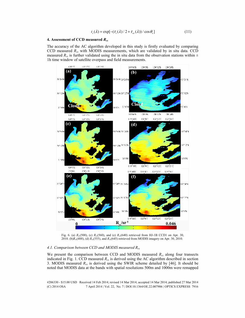
r s( ) exp[ ( ( ) / 2 ( )) / cos ]s ozt λ τ λ τ λ θ= − + (11)

4. Assessment of CCD measured Rrs

The accuracy of the AC algorithm developed in this study is firstly evaluated by comparing CCD measured Rrs with MODIS measurements, which are validated by in situ data. CCD measured Rrs is further validated using the in situ data from the observation stations within ± 1h time window of satellite overpass and field measurements.

Fig. 6. (a) Rrs(500), (c) Rrs(560), and (e) Rrs(640) retrieved from HJ-1B CCD1 on Apr. 30, 2010. (b)Rrs(488), (d) Rrs(555), and Rrs(645) retrieved from MODIS imagery on Apr. 30, 2010.

4.1. Comparison between CCD and MODIS measured Rrs

We present the comparison between CCD and MODIS measured Rrs along four transects indicated in Fig. 1. CCD measured Rrs is derived using the AC algorithm described in section 3. MODIS measured Rrs is derived using the SWIR scheme detailed by [46]. It should be noted that MODIS data at the bands with spatial resolutions 500m and 1000m were remapped


with 250m by means of the bilinear interpolation method for the two lakes with relatively small area.

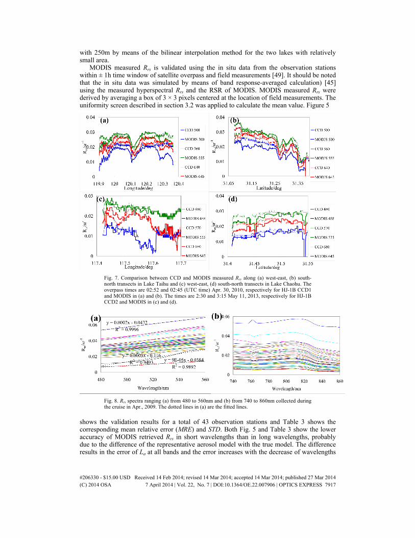
MODIS measured Rrs is validated using the in situ data from the observation stations within ± 1h time window of satellite overpass and field measurements [49]. It should be noted that the in situ data was simulated by means of band response-averaged calculation) [45] using the measured hyperspectral Rrs and the RSR of MODIS. MODIS measured Rrs were derived by averaging a box of 3 × 3 pixels centered at the location of field measurements. The uniformity screen described in section 3.2 was applied to calculate the mean value. Figure 5

Fig. 7. Comparison between CCD and MODIS measured Rrs along (a) west-east, (b) south-north transects in Lake Taihu and (c) west-east, (d) south-north transects in Lake Chaohu. The overpass times are 02:52 and 02:45 (UTC time) Apr. 30, 2010, respectively for HJ-1B CCD1 and MODIS in (a) and (b). The times are 2:30 and 3:15 May 11, 2013, respectively for HJ-1B CCD2 and MODIS in (c) and (d).

Fig. 8. Rrs spectra ranging (a) from 480 to 560nm and (b) from 740 to 860nm collected during the cruise in Apr., 2009. The dotted lines in (a) are the fitted lines.

shows the validation results for a total of 43 observation stations and Table 3 shows the corresponding mean relative error (MRE) and STD. Both Fig. 5 and Table 3 show the lower accuracy of MODIS retrieved Rrs in short wavelengths than in long wavelengths, probably due to the difference of the representative aerosol model with the true model. The difference results in the error of La at all bands and the error increases with the decrease of wavelengths


[4]. The lower accuracy is also possibly due to the significant degradation at blue bands. The degradation is a common occurrence as satellite instruments age in the harsh space environment. It was reported that the degradation at short wavelengths is larger than at long wavelengths for Terra MODIS [50]. It is noted from Fig. 5 the tendency of smaller MODIS measured Rrs than in situ data, which is probably resulted from the small ρ (0.025 in the study) used in calculating the in situ Rrs. It was reported that ρ increases from 0.026 with wind speed 0m/s to approximately 0.043 when wind speed is 15m/s under the assumption of a viewing zenith and azimuth angles about 40° and 135° and a clear-sky radiance distribution for θs about 30° [28]. The small ρ results in the higher Rrs than the true value. It is noted from [29] that the relative difference between Rrs calculated using ρ equivalent to 0.022 and 0.034

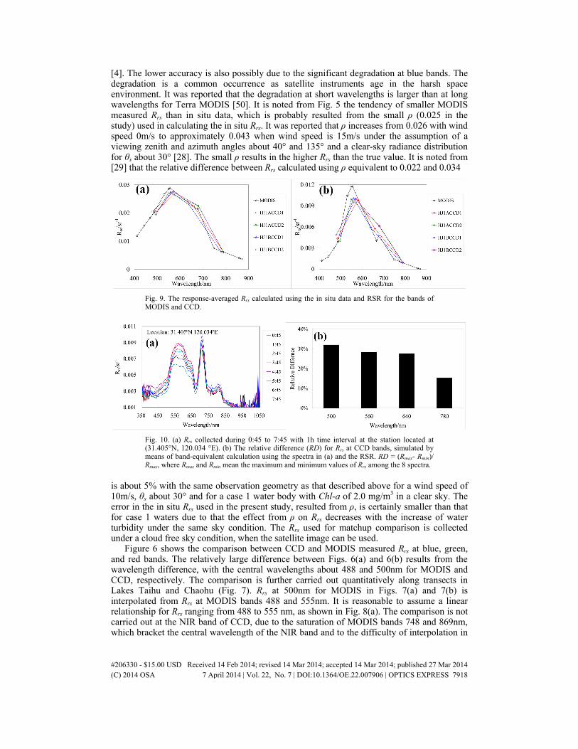
Fig. 9. The response-averaged Rrs calculated using the in situ data and RSR for the bands of MODIS and CCD.

Fig. 10. (a) Rrs collected during 0:45 to 7:45 with 1h time interval at the station located at (31.405°N, 120.034 °E). (b) The relative difference (RD) for Rrs at CCD bands, simulated by means of band-equivalent calculation using the spectra in (a) and the RSR. RD = (Rmax- Rmin)/ Rmax, where Rmax and Rmin mean the maximum and minimum values of Rrs among the 8 spectra.

is about 5% with the same observation geometry as that described above for a wind speed of 10m/s, θs about 30° and for a case 1 water body with Chl-a of 2.0 mg/m3 in a clear sky. The error in the in situ Rrs used in the present study, resulted from ρ, is certainly smaller than that for case 1 waters due to that the effect from ρ on Rrs decreases with the increase of water turbidity under the same sky condition. The Rrs used for matchup comparison is collected under a cloud free sky condition, when the satellite image can be used.

Figure 6 shows the comparison between CCD and MODIS measured Rrs at blue, green, and red bands. The relatively large difference between Figs. 6(a) and 6(b) results from the wavelength difference, with the central wavelengths about 488 and 500nm for MODIS and CCD, respectively. The comparison is further carried out quantitatively along transects in Lakes Taihu and Chaohu (Fig. 7). Rrs at 500nm for MODIS in Figs. 7(a) and 7(b) is interpolated from Rrs at MODIS bands 488 and 555nm. It is reasonable to assume a linear relationship for Rrs ranging from 488 to 555 nm, as shown in Fig. 8(a). The comparison is not carried out at the NIR band of CCD, due to the saturation of MODIS bands 748 and 869nm, which bracket the central wavelength of the NIR band and to the difficulty of interpolation in


the wavelength range of 740 to 860nm as shown in Fig. 8(b). Figure 7 shows a better consistency at red and green bands than at blue bands. The difference between CCD and MODIS measured Rrs results from the difference of RSR (as shown in Fig. 2). The effect of the RSR difference is shown in Fig. 9, where the Rrs spectra are derived by means of band-equivalent calculation method using the RSR and in situ data. The difference in Fig. 7 is also possibly due to the spatial variation resulted from the uncertainties in geometric positioning and the temporal variation since the color of the shallow water with a mean depth about 1.9m [51] is easily affected by wind-driven resuspension. In order to evaluate the stability of the water color in Lake Taihu, the spectra were collected with 1h time interval from 0:45 to 7:45 (UTC time) on May 2, 2010 at the station located at (31.405°N, 120.034 °E). The spectra variation is shown in Fig. 10, from which we can see that the variation may reach 30% during

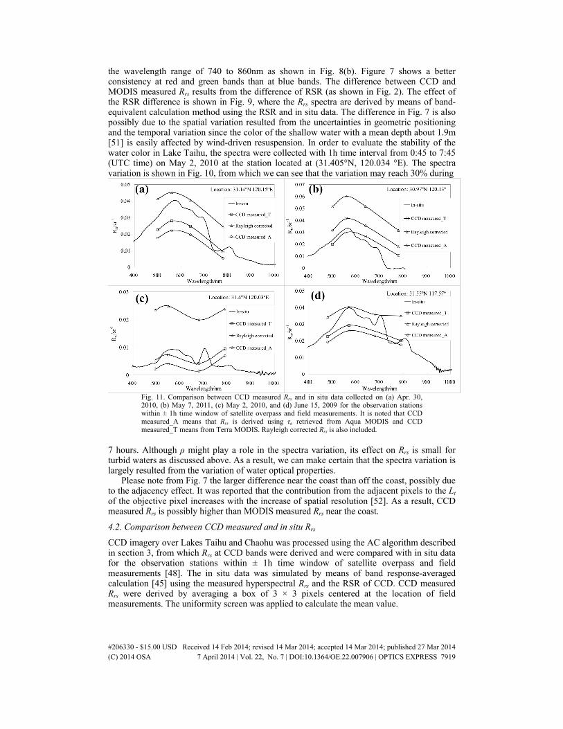
Fig. 11. Comparison between CCD measured Rrs and in situ data collected on (a) Apr. 30, 2010, (b) May 7, 2011, (c) May 2, 2010, and (d) June 15, 2009 for the observation stations within ± 1h time window of satellite overpass and field measurements. It is noted that CCD measured_A means that Rrs is derived using τa retrieved from Aqua MODIS and CCD measured_T means from Terra MODIS. Rayleigh corrected Rrs is also included.

7 hours. Although ρ might play a role in the spectra variation, its effect on Rrs is small for turbid waters as discussed above. As a result, we can make certain that the spectra variation is largely resulted from the variation of water optical properties.

Please note from Fig. 7 the larger difference near the coast than off the coast, possibly due to the adjacency effect. It was reported that the contribution from the adjacent pixels to the Lt of the objective pixel increases with the increase of spatial resolution [52]. As a result, CCD measured Rrs is possibly higher than MODIS measured Rrs near the coast.

4.2. Comparison between CCD measured and in situ Rrs

CCD imagery over Lakes Taihu and Chaohu was processed using the AC algorithm described in section 3, from which Rrs at CCD bands were derived and were compared with in situ data for the observation stations within ± 1h time window of satellite overpass and field measurements [48]. The in situ data was simulated by means of band response-averaged calculation [45] using the measured hyperspectral Rrs and the RSR of CCD. CCD measured Rrs were derived by averaging a box of 3 × 3 pixels centered at the location of field measurements. The uniformity screen was applied to calculate the mean value.


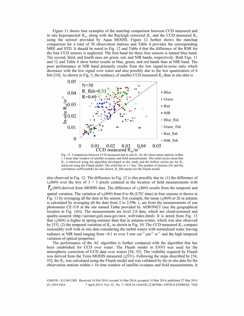
Figure 11 shows four examples of the matchup comparison between CCD measured and in situ hyperspectral Rrs, along with the Rayleigh corrected Rrs and the CCD measured Rrs using the aerosol provided by Aqua MODIS. Figure 12 further shows the matchup comparison for a total of 30 observation stations and Table 4 provides the corresponding MRE and STD. It should be noted in Fig. 12 and Table 4 that the difference of the RSR for the four CCD sensors is neglected. The first band for these four sensors is named blue band. The second, third, and fourth ones are green, red, and NIR bands, respectively. Both Figs. 11 and 12 and Table 4 show better results at blue, green, and red bands than at NIR band. The poor performance at NIR band primarily results from the low signal-to-noise ratio which decreases with the low signal over water and also possibly due to the low quantization of 8 bits [10]. As shown in Fig. 5, the tendency of smaller CCD measured Rrs than in situ data is

Fig. 12. Comparison between CCD measured and in situ Rrs for the observation stations within ± 1 hour time window of satellite overpass and field measurements. The solid circles mean that Rrs is retrieved using the algorithm developed in this study and the hollow circles are for Rrs retrieved using the Flaash model. The solid line is 1:1 line. The number of stations (N) and the correlation coefficient(R) are also shown. R_flsh means for the Flaash model.

also observed in Fig. 12. The difference in Fig. 12 is also possibly due to: (1) the difference of τa(869) over the box of 3 × 3 pixels centered at the location of field measurements with

(869)aτ derived from MODIS data. The difference of τa(869) results from the temporal and

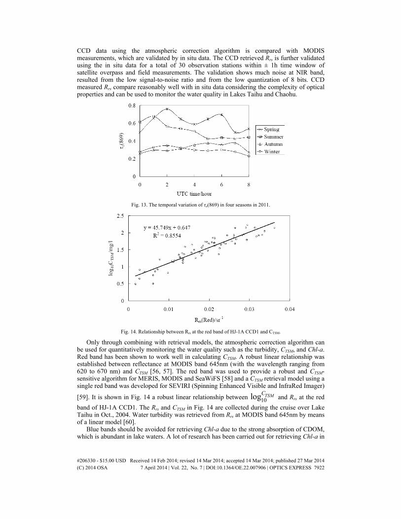
spatial variation. The variation of τa(869) from 0 to 8h (UTC time) in four seasons is shown in Fig. 13 by averaging all the data in the season. For example, the mean τa(869) at 2h in autumn is calculated by averaging all the data from 2 to 2:59h. τa are from the measurements of sun photometer CE-318 at the site named Taihu provided by AERONET (see the geographical location in Fig. 1(b)). The measurements are level 2.0 data, which are cloud-screened and quality-assured (http://aeronet.gsfc.nasa.gov/new_web/index.html). It is noted from Fig. 13 that τa(869) is higher in spring-summer than that in autumn-winter, which was also observed by [53]. (2) the temporal variation of Rrs as shown in Fig. 10. The CCD measured Rrs compare reasonably well with in situ data considering the turbid waters with normalized water leaving radiance at NIR band ranging from ~0.1 to over 5 mw cm−2 μm−1 sr−1 and the high temporal variation of optical properties.

The performance of the AC algorithm is further compared with the algorithm that has been established for CCD over water. The Flaash model in ENVI was used for the atmospheric correction of CCD data over waters [54, 55]. The visibility required by Flaash was derived from the Terra MODIS measured τa(551). Following the steps described by [54, 55], the Rrs was calculated using the Flaash model and was validated by the in situ data for the observation stations within ± 1h time window of satellite overpass and field measurements. It


is noted that τa(551) is retrieved from MODIS using the AC algorithm presented by [46]. Both Fig. 12 and Tables 4 and 5 show that the algorithm developed in this study has a better performance than the Flaash model.

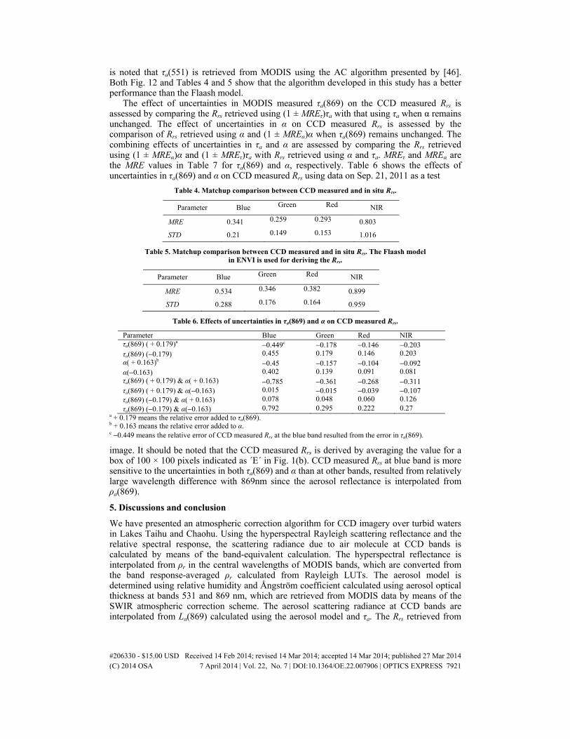
The effect of uncertainties in MODIS measured τa(869) on the CCD measured Rrs is assessed by comparing the Rrs retrieved using (1 ± MREτ)τa with that using τa when α remains unchanged. The effect of uncertainties in α on CCD measured Rrs is assessed by the comparison of Rrs retrieved using α and (1 ± MREα)α when τa(869) remains unchanged. The combining effects of uncertainties in τa and α are assessed by comparing the Rrs retrieved using (1 ± MREα)α and (1 ± MREτ)τa with Rrs retrieved using α and τa. MREτ and MREα are the MRE values in Table 7 for τa(869) and α, respectively. Table 6 shows the effects of uncertainties in τa(869) and α on CCD measured Rrs using data on Sep. 21, 2011 as a test

Table 4. Matchup comparison between CCD measured and in situ Rrs.

Parameter Blue Green Red NIR

MRE 0.341 0.259 0.293 0.803

STD 0.21 0.149 0.153 1.016

Table 5. Matchup comparison between CCD measured and in situ Rrs. The Flaash model in ENVI is used for deriving the Rrs.

Parameter Blue Green Red NIR

MRE 0.534 0.346 0.382 0.899

STD 0.288 0.176 0.164 0.959

Table 6. Effects of uncertainties in τa(869) and α on CCD measured Rrs.

Parameter Blue Green Red NIR τa(869) ( + 0.179)a −0.449c −0.178 −0.146 −0.203 τa(869) (−0.179) 0.455 0.179 0.146 0.203 α( + 0.163)b −0.45 −0.157 −0.104 −0.092 α(−0.163) 0.402 0.139 0.091 0.081 τa(869) ( + 0.179) & α( + 0.163) −0.785 −0.361 −0.268 −0.311 τa(869) ( + 0.179) & α(−0.163) 0.015 −0.015 −0.039 −0.107 τa(869) (−0.179) & α( + 0.163) 0.078 0.048 0.060 0.126 τa(869) (−0.179) & α(−0.163) 0.792 0.295 0.222 0.27

a + 0.179 means the relative error added to τa(869). b + 0.163 means the relative error added to α. c −0.449 means the relative error of CCD measured Rrs at the blue band resulted from the error in τa(869).

image. It should be noted that the CCD measured Rrs is derived by averaging the value for a box of 100 × 100 pixels indicated as ´E´ in Fig. 1(b). CCD measured Rrs at blue band is more sensitive to the uncertainties in both τa(869) and α than at other bands, resulted from relatively large wavelength difference with 869nm since the aerosol reflectance is interpolated from ρa(869).

5. Discussions and conclusion

We have presented an atmospheric correction algorithm for CCD imagery over turbid waters in Lakes Taihu and Chaohu. Using the hyperspectral Rayleigh scattering reflectance and the relative spectral response, the scattering radiance due to air molecule at CCD bands is calculated by means of the band-equivalent calculation. The hyperspectral reflectance is interpolated from ρr in the central wavelengths of MODIS bands, which are converted from the band response-averaged ρr calculated from Rayleigh LUTs. The aerosol model is determined using relative humidity and Ångström coefficient calculated using aerosol optical thickness at bands 531 and 869 nm, which are retrieved from MODIS data by means of the SWIR atmospheric correction scheme. The aerosol scattering radiance at CCD bands are interpolated from La(869) calculated using the aerosol model and τa. The Rrs retrieved from


CCD data using the atmospheric correction algorithm is compared with MODIS measurements, which are validated by in situ data. The CCD retrieved Rrs is further validated using the in situ data for a total of 30 observation stations within ± 1h time window of satellite overpass and field measurements. The validation shows much noise at NIR band, resulted from the low signal-to-noise ratio and from the low quantization of 8 bits. CCD measured Rrs compare reasonably well with in situ data considering the complexity of optical properties and can be used to monitor the water quality in Lakes Taihu and Chaohu.

Fig. 13. The temporal variation of τa(869) in four seasons in 2011.

Fig. 14. Relationship between Rrs at the red band of HJ-1A CCD1 and CTSM.

Only through combining with retrieval models, the atmospheric correction algorithm can be used for quantitatively monitoring the water quality such as the turbidity, CTSM, and Chl-a. Red band has been shown to work well in calculating CTSM. A robust linear relationship was established between reflectance at MODIS band 645nm (with the wavelength ranging from 620 to 670 nm) and CTSM [56, 57]. The red band was used to provide a robust and CTSM-sensitive algorithm for MERIS, MODIS and SeaWiFS [58] and a CTSM retrieval model using a single red band was developed for SEVIRI (Spinning Enhanced Visible and InfraRed Imager)

[59]. It is shown in Fig. 14 a robust linear relationship between 10log TSMC and Rrs at the red

band of HJ-1A CCD1. The Rrs and CTSM in Fig. 14 are collected during the cruise over Lake Taihu in Oct., 2004. Water turbidity was retrieved from Rrs at MODIS band 645nm by means of a linear model [60].

Blue bands should be avoided for retrieving Chl-a due to the strong absorption of CDOM, which is abundant in lake waters. A lot of research has been carried out for retrieving Chl-a in


case 2 waters using red and NIR bands [61]. established a three-band reflectance model for assessing Chl-a in turbid productive waters. Two red bands in the range of 670-700nm and one NIR band around 750nm are used in the model. Using measured Rrs and Chl-a, three bands with central wavelengths 666, 688, and 725nm were selected by means of optimization and iteration for retrieving Chl-a in Lake Taihu [62]. An improved four-band model had a better performance than the three-band model when applied to Lake Taihu [63]. The central wavelengths for the four bands are 663, 693, 705, and 740nm. Overall, at least two red bands

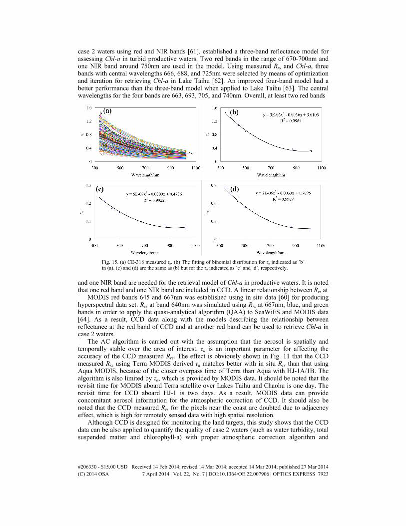
Fig. 15. (a) CE-318 measured τa. (b) The fitting of binomial distribution for τa indicated as ´b´ in (a). (c) and (d) are the same as (b) but for the τa indicated as ´c´ and ´d´, respectively.

and one NIR band are needed for the retrieval model of Chl-a in productive waters. It is noted that one red band and one NIR band are included in CCD. A linear relationship between Rrs at

MODIS red bands 645 and 667nm was established using in situ data [60] for producing hyperspectral data set. Rrs at band 640nm was simulated using Rrs at 667nm, blue, and green bands in order to apply the quasi-analytical algorithm (QAA) to SeaWiFS and MODIS data [64]. As a result, CCD data along with the models describing the relationship between reflectance at the red band of CCD and at another red band can be used to retrieve Chl-a in case 2 waters.

The AC algorithm is carried out with the assumption that the aerosol is spatially and temporally stable over the area of interest. τa is an important parameter for affecting the accuracy of the CCD measured Rrs. The effect is obviously shown in Fig. 11 that the CCD measured Rrs using Terra MODIS derived τa matches better with in situ Rrs than that using Aqua MODIS, because of the closer overpass time of Terra than Aqua with HJ-1A/1B. The algorithm is also limited by τa, which is provided by MODIS data. It should be noted that the revisit time for MODIS aboard Terra satellite over Lakes Taihu and Chaohu is one day. The revisit time for CCD aboard HJ-1 is two days. As a result, MODIS data can provide concomitant aerosol information for the atmospheric correction of CCD. It should also be noted that the CCD measured Rrs for the pixels near the coast are doubted due to adjacency effect, which is high for remotely sensed data with high spatial resolution.

Although CCD is designed for monitoring the land targets, this study shows that the CCD data can be also applied to quantify the quality of case 2 waters (such as water turbidity, total suspended matter and chlorophyll-a) with proper atmospheric correction algorithm and


retrieval models, providing useful information for decision makers to manage water environment and to prepare for events as algal blooms.

Appendix A. Validation of the Terra MODIS measured τa

It should be noted that τa retrieved from MODIS is critical to the atmospheric correction of CCD imagery. τa at bands 531 and 869nm are used to calculate the Ångström coefficient which is used along with the relative humidity to determine the aerosol model. Using the aerosol model and τa(869), ρa(869) is derived, from which the reflectance at CCD bands are

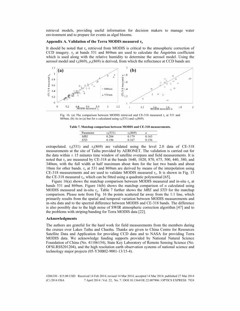
Fig. 16. (a) The comparison between MODIS retrieved and CE-318 measured τa at 531 and 869nm. (b) As in (a) but for α calculated using τa(531) and τa(869).

Table 7. Matchup comparison between MODIS and CE-318 measurements.

Parameter τa(531) τa(869) αMRE 0.204 0.179 0.163STD 0.196 0.167 0.156

extrapolated. τa(531) and τa(869) are validated using the level 2.0 data of CE-318 measurements at the site of Taihu provided by AERONET. The validation is carried out for the data within ± 15 minutes time window of satellite overpass and field measurements. It is noted that τa are measured by CE-318 at the bands 1640, 1020, 870, 675, 500, 440, 380, and 340nm, with the full width at half maximum about 4nm for the last two bands and about 10nm for other bands. τa at 531 and 869nm are derived by means of the interpolation using CE-318 measurements and are used to validate MODIS measured τa. It is shown in Fig. 15 the CE-318 measured τa, which can be fitted using a quadratic polynomial [65].

Figure 16(a) shows the matchup comparison between MODIS measured and in-situ τa at bands 531 and 869nm. Figure 16(b) shows the matchup comparison of α calculated using MODIS measured and in-situ τa. Table 7 further shows the MRE and STD for the matchup comparison. Please note from Fig. 16 the points scattered far away from the 1:1 line, which primarily results from the spatial and temporal variation between MODIS measurements and in-situ data and to the spectral difference between MODIS and CE-318 bands. The difference is also possibly due to the high noise of SWIR atmospheric correction algorithm [47] and to the problems with striping/banding for Terra MODIS data [22].

Acknowledgments

The authors are grateful for the hard work for field measurements from the members during the cruises over Lakes Taihu and Chaohu. Thanks are given to China Centre for Resources Satellite Data and Application for providing CCD data and to NASA for providing Terra MODIS data. We acknowledge funding supports provided by National Natural Science Foundation of China (No. 41106154), State Key Laboratory of Remote Sensing Science (No. OFSLRSS201204), and the high resolution earth observation systems of national science and technology major projects (05-Y30B02-9001-13/15-4).


atmospheric correction of hj-1 ccd imagery over turbid ... · atmospheric correction of hj-1 ccd...

Documents