atmospheric boundary layer height monitoring using a kalman filter and backscatter lidar returns

IEEE TRANSACTIONS ON GEOSCIENCE AND REMOTE SENSING, VOL. 52, NO. 8, AUGUST 2014 4717

Atmospheric Boundary Layer Height MonitoringUsing a Kalman Filter and Backscatter

Lidar ReturnsDiego Lange, Jordi Tiana-Alsina, Umar Saeed, Sergio Tomás, and Francesc Rocadenbosch, Member, IEEE

Abstract—A solution based on a Kalman filter to trace theevolution of the atmospheric boundary layer (ABL) sensed by aground-based elastic-backscatter tropospheric lidar is presented.An erf-like profile is used to model the mixing-layer top and theentrainment-zone thickness. The extended Kalman filter (EKF)enables to retrieve and track the ABL parameters based on sim-plified statistics of the ABL dynamics and of the observation noisepresent in the lidar signal. This adaptive feature permits to analyzeatmospheric scenes with low signal-to-noise ratios (SNRs) withoutthe need to resort to long-time averages or range-smoothing tech-niques, as well as to pave the way for future automated detectionsolutions. First, EKF results based on oversimplified syntheticand experimental lidar profiles are presented and compared withclassic ABL estimation quantifiers for a case study with differentSNR scenarios.

Index Terms—Adaptive kalman filtering, laser radar, remotesensing, signal processing.

I. INTRODUCTION

THERE are several methods to retrieve the atmosphericboundary layer (ABL) height based on remote sensing

techniques. These techniques are always based on the detec-tion of a vertical feature from atmospheric variables, whichcontinuously vary with range and time, and having a well-defined transition identifiable as an “edge” or “boundary.”Height retrieval methods and their accuracy are conditionedto the characteristics of the sensing instrumentation: lidar,sodar, radar wind profilers, and radio acoustic sounding system,among others (see [1] for an extensive review), either solely orcombined [2].

A significant advantage of backscatter lidar remote sensinginstruments is that they are able to gather a range-resolvedprofile of the ABL simultaneously for the whole observationrange, which greatly improves the temporal resolution of in situsensors and radiosoundings.

Manuscript received June 19, 2013; revised August 7, 2013; acceptedSeptember 13, 2013. Date of publication October 24, 2013; date of currentversion February 27, 2014.

D. Lange and F. Rocadenbosch are with the Department of Signal Theoryand Communications (TSC), Remote Sensing Laboratory (RSLab), UniversitatPolitècnica de Catalunya (UPC)/Institut d’Estudis Espacials de Catalunya(IEEE/CRAE), 08034 Barcelona, Spain (e-mail: [email protected]).

J. Tiana-Alsina and U. Saeed are with the Department of Signal Theoryand Communications (TSC), Remote Sensing Laboratory (RSLab), UniversitatPolitècnica de Catalunya (UPC), 08034 Barcelona, Spain.

S. Tomás is with the Institut de Ciències de l’Espai-Consejo Superior de In-vestigaciones Científicas/Institut d’Estudis Espacials de Catalunya (ICE-CSIC/IEEC), 08193 Barcelona, Spain.

Digital Object Identifier 10.1109/TGRS.2013.2284110

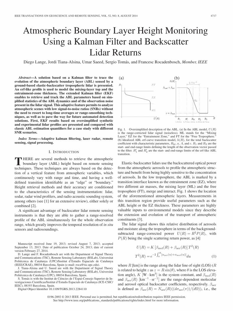
Fig. 1. Oversimplified description of the ABL. (a) In the ABL model, U(R)is the range-corrected lidar signal (noiseless). ML stands for the “MixingLayer,” EZ for the “Entrainment Zone,” and FT for the “Free Troposphere.”(b) Idealized ABL erf-curve transition model, h(R), for the total backscattercoefficient with characteristic parameters, Rbl, a, A, and c. R1 and R2 are thestart- and end-range limits defining the length of the observation vector passedto the filter. R′

1 and R′2 are the start- and end-range limits of the erf-like ABL

transition.

Elastic-backscatter lidars use the backscattered optical powerfrom the atmospheric aerosols to profile the atmospheric struc-ture and benefit from being highly sensitive to the concentrationof aerosols. In the low troposphere, the ABL is marked by atransition interface known as the entrainment zone (EZ), wheretwo different air masses, the mixing layer (ML) and the freetroposphere (FT), merge and interact. Fig. 1 shows the locationof the aforementioned atmospheric layers. Measurements inthis transition region provide useful parameters such as theABL height or the EZ thickness. These parameters are highlyvaluable inputs to environmental models since they describethe extension and evolution of the transport of atmosphericconstituents [3].

The lidar signal shows this relative distribution of aerosolsand moisture along the troposphere in terms of the background-subtracted range-corrected power U(R) = R2P (R), withP (R) being the single scattering return power, as [4]

U(R) =K [βmol(R) + βaer(R)]T 2(R)

T 2(R) = e−2

∫ R

0[αaer(u)+αmol(u)]du (1)

where R [km] is the range along the lidar line of sight (LOS) (Ris related to height z as z = R sin(θ), where θ is the LOS eleva-tion angle), K [W · km3] is the system constant, and βmol(R)and βaer(R) [km−1 · sr−1] are the range-dependent molecularand aerosol optical backscatter coefficients, respectively. βaer

is defined as βaer(R) = Naer(R)((dσaer(π))/(dΩ)), i.e., the

0196-2892 © 2013 IEEE. Personal use is permitted, but republication/redistribution requires IEEE permission.See http://www.ieee.org/publications_standards/publications/rights/index.html for more information.

4718 IEEE TRANSACTIONS ON GEOSCIENCE AND REMOTE SENSING, VOL. 52, NO. 8, AUGUST 2014

product of the aerosol number concentration, N(R)aer [km−3],and the average differential backscatter cross section of theaerosol mixture, ((dσaer(π))/(dΩ) [km2 · sr−1], which in-cludes the effects of aerosol type and moisture. The molecularcomponent, βmol(R), can be computed from the U.S. standardatmosphere model [5] or radiosoundings.

Finally, T 2(R) represents the two-way path atmospherictransmittance affecting the optical pulse, with αmol and αaer

being the atmospheric extinction coefficients due to aerosolsand molecules, respectively.

The transmittance factor can be included into the totalbackscatter by defining the attenuated total backscatter as

βatten(R) = β(R)T 2(R) (2)

where β(R) = βmol(R) + βaer(R). Inside the ML and, par-ticularly, toward the NIR or in relatively optically denseatmospheres, the aerosol backscatter component dominates, soβaer(R) � βmol(R) and β(R) ≈ βaer(R). This simplificationmakes the range-corrected lidar signal, U(R), almost propor-tional to the aerosol number concentration profile, Naer(R). Incontrast, in the FT, the aerosol content is virtually nil (withthe exception of, e.g., unstable dust layers or dust intrusions[6]), and hence, β(R) ≈ βmol(R). As a result, in the FT, thelidar signal, U(R), becomes proportional to the profile of themolecular number concentration, Nmol(R) (see Fig. 1).

The lidar profile typically presents a sharp decrease at someheight inside the EZ, henceforth called the ABL local transition.The buoyancy-driven updrafts tend to narrow this local transi-tion, while in the case of downdrafts, the transition widens [7].This simple assumption of aerosol concentration/lidar signalpreviously mentioned is often distorted by several factors suchas instrumental noise, multilayer scenarios (transported layers,stratified layers, lateral entrainments, or the residual layer),and nonlinear effects of moisture distribution in the aerosolbackscatter. The influence of all these effects is different, de-pending on which method of ABL height detection is chosen.Thus, active research in terms of intercomparison is still underway [8], [9].

Lidar sensing of the ABL has been carried out not only byground-based systems such as backscatter lidars [10], water-vapor differential absorption lidar [11], or, more recently,ceilometers [12] but also by airborne lidars [13] and scanninglidars in a range height indicator scan [14], [15]. Ground-fixedsystems monitor the ABL structure as a function of time whileairborne and scanning lidars spatially assess the ABL. Twodifferent approaches to estimate the ABL height from lidarsignals can be outlined:

1) The geometrical approach uses the fact that the EZ regionusually appears in the individual lidar signal profiles as asharp decrease between the two air masses (this is due tothe lack of aerosols and moisture in the FT, all of whichcause a strong signature in the range-corrected backscat-ter lidar return). Geometrical-based ABL-detectionmethods rely on the detection of a meaningful transition,usually by some sort of edge-detection analysis, by meansof a threshold criterion [13], [16], [17] or gradient detec-tion [10], [18] applied to time-averaged profiles. When

high signal-to-noise ratio (SNR) and temporal resolutionare available from the lidar sensor, geometrical methodsare able to retrieve the instantaneous ABL height (hABL),which is identified as the instantaneous ABL top.

2) The statistical approach uses the high variability in thereturn signal caused by the mixing processes betweencells in the EZ and cells in the FT above or in the MLbelow. This approach requires the analysis of a set ofprofiles to produce a statistically significant estimate ofthe ML depth, taken as the mean ABL height (hABL).

In this paper, we present a tradeoff between both aforemen-tioned approaches by using an adaptive filter solution basedon the extended Kalman filter (EKF) [19] which estimatesthe time-dependent ABL height, hABL, the approximate EZthickness, and auxiliary atmospheric backscatter-coefficient pa-rameters. A preliminary study on the problem has been outlinedin [20], from the Remote Sensing Laboratory (RSLab). Becausethe filter adaptively fits a model shape function to the lidar-measured data and minimizes the mean-squared error over timein a statistical sense, it provides convenient estimates. Thefilter thus makes the most from the high temporal resolution ofcurve-fitting geometrical models and the physically significantestimate output by statistical methods.

In the concept-design implementation of the filter presentedhere, multilayer scenes are not considered. In contrast, this pa-per focuses on the impact that noise has on the filter estimates,particularly for different SNR scenarios.

This paper is organized as follows: Section II formulatesthe nonlinear adaptive estimator based on the Kalman filtertheory with which ABL parameters can sensibly be estimated.Section III shows the simulation results on the temporal evo-lution of the ABL parameters and cross-examines them withthe estimated ones from EKF and traditional nonlinear leastsquares (NLSQ) approaches. Section IV presents the results ofapplying the EKF approach to experimental lidar backscatterdata under two different SNR scenarios (high and low SNRs).Results are also compared with well-known classical ABL-detection methods in the literature. Finally, concluding resultsare presented in Section V.

II. ABL ADAPTIVE DETECTION METHOD

An EKF is applied to adaptively fit an erf-like functionmodeling the EZ lidar-signal transition curve to the range-corrected lidar measurements. The erf curve-fitting method [21]is chosen because it is a robust approach which involves thebulk of the lidar profile. Later studies have been given in [7]and [22], mostly on the convective boundary layer (CBL).

The application of the EKF to the field of lidar-signal pro-cessing to estimate the atmospheric optical parameters departsfrom previous works in [23] and [24]. On the other hand,Mukherjee et al. [25] have applied a scalar Kalman filter toestimate the ABL height from sodar signals.

A. EKF Approach

The discrete Kalman filter is an adaptive linear estimatorinherited from control system theory that operates recursively

LANGE et al.: ABL HEIGHT MONITORING USING KALMAN FILTER AND BACKSCATTER LIDAR RETURNS 4719

using a state-space model formulation. The filter is based ontwo models: 1) the measurement model (see Section II-C1),which relates the atmospheric state-vector unknowns (to beestimated) to the observation measurements (i.e., the range-corrected lidar backscatter signals), and 2) the state-vectormodel (see Section II-C2), which approximately describes thetemporal projection of the unknowns and its associated statis-tics [see (5)]. However poor this “a priori” information aboutthe atmospheric state vector and its statistics may be, thisinformation is of advantage to the filter in order to improve itsestimates by combining the actual estimation with the statisticalbehavior from past estimates. In what follows, “a priori” and“a posteriori” stand for “before” and “after” assimilating theinformation from the present measurement at discrete time tk,respectively.

When, as is the case of (1), the measurement model is non-linear, a linearization is made around the state-vector trajectory,which is updated at each successive iteration of the filter oncea new measurement zk is assimilated in what is called theEKF. Likewise, at each filter iteration, the state vector, xk, theestimated a priori and a posteriori error-covariance matrices,P−

k and Pk, respectively, and the Kalman gain, Kk, are recur-sively updated (see, e.g., [19, pp. 215–219] and [24]). By therecursive procedure, the filter corrects its projection trajectoryof the ABL atmospheric variables and improves its estimationof the ABL parameters via a new atmospheric state vector xk

being estimated. By means of this convenient adaptive behavior,tracking the state-vector components appears as a natural anddesirable feature of the filter.

For an M -component state vector (M = 4 in the case ofthe ABL estimation model described in Section II-C1), thenumber of observation samples in the ABL transition (N) mustobviously be N ≥ M for data sufficiency. In practice, a muchlarger number of samples—as it is always the case—conveysthe extra benefit of enhanced robustness to noise (this is equiva-lent to an overdetermined system of equations in classic algebratheory).

B. ABL Problem Formulation

For moderate to clear-air atmospheres and lidar soundingranges roughly below 3 km (R ≤ 3 km), the optical thickness,τ =

∫ R

0 [αaer(u) + αmol(u)]du, can be considered low enough(τ < 1) to disregard the effects of the atmospheric transmissiv-ity term T (R) in (1). Under these conditions usually found inpractice, the range-corrected lidar signal, U(R), is proportionalto the total backscatter coefficient in (1)

U(R) � Kβ(R) (3)

with β(R) = βaer(R) + βmol(R). As a result, U(R) can beconsidered a surrogate for the total backscatter coefficientβ(R), which is representative of the average aerosol and molec-ular concentration of the atmospheric mixture aloft.

The range-corrected lidar signal exhibits a transition curvefrom high concentrations inside the ABL to lower concentra-tions (molecular-background level) as the height increases. TheABL transition model proposed here follows a similar formu-lation to that in [21] but for the total backscatter coefficient.

The erf-like total backscatter-coefficient model is formulated interms of four characteristic parameters, Rbl, a, A, and c, as

h(R;Rbl, a, A, c) =A

2

{1− erf

[a√2(R−Rbl)

]}+ c (4)

where Rbl is the range position that marks the instantaneousABL height, defined as the inflection point where the function hchanges from convex to concave (equivalently, the point whereh has minimum gradient), a is a scaling factor related to thetransition thickness, A is the total backscatter-coefficient tran-sition amplitude (equivalently, the difference between the upperand lower asymptotical levels of h or between the ML and FTbackscatter-related values), and c is an offset term modelingthe FT molecular-backscatter level. Equation (4) models anidealized CBL profile consisting of a single transition structurebetween the ML and the FT within the range interval [R1, R2][see Fig. 1(b)].

In (4), the key parameters of interest are Rbl and a for theyare directly related to the measurements of the ML depth andto the EZ thickness [7]. The instantaneous ML top is identifiedas the minimum-gradient model parameter, Rbl[26]. For an erf-based ABL transition, its derivative is a Gaussian curve whosefull-width half maximum, σbl, is related to a as a−1 =

√2σbl

(see Fig. 1). Following [21], the 95-to-5% falling transitionthickness is 2.77a−1.

From the physical point of view, the variation of the local-transition scale factor a with time comes as a function ofthe variation of the EZ thickness (i.e., a varies as the localtransitions caused by updrafts and downdrafts). The variabilityof the amplitude of the ML with respect to the molecular level[A in (13)] is caused by the entrainments of aerosol structuresas they cross the lidar beam and is dependent on the normalizedbackscatter values of these structures, their size, their advectionvelocity, and the time resolution of the lidar acquisition.

In the adaptive approach proposed next, the EKF filter con-siders the four characteristic parameters of the (4) model astime-variant stochastic processes forming the state vector to beestimated at each time tk

xk = [Rbl,k, ak, Ak, ck]t (5)

here given in transposed form.The EKF observation vector, zk, is related to the state vector,

xk, via the measurement model

zk = h(xk) + vk (6)

where h is the ABL transition model of (4) and vk is theobservation noise at time tk (including both lidar instrumentnoise and modeling errors) with associated noise covariancematrix Rk (see [19, p. 215]). In (6), the observation vector zk(i.e., the lidar measurements at each time tk) is the measurednoise-corrupted version of h(R) in the range interval [R1, R2].

As mentioned in Section II-B, under moderate-to-low opticalthickness (τ < 1), the range-corrected lidar signal U(R) isbasically proportional to the total backscatter coefficient.

For better numerical conditioning and physical significance,the observation vector zk presented to the filter is a molecular


normalized version of U(R), zk = Un(Rk), as described in theAppendix. This is basically saying that Un(R) � βmol(R) +βaer(R) in (1), which is in accordance to Fig. 1 (in [R1, R

′1],

h(R) tends to βmol+βaer, and in [R′2, R2], h(R) tends to βmol).

C. Filter Models

Measurement Model: In the EKF approach, at each succes-sive time tk, the filter compares the actual observable zk formedfrom the measured normalized lidar signal [see (25)] with alinearized version of the observation model, Hk. The latteris based on the partial derivatives of the measurement-modelfunction h(R) [see (4)] evaluated at the “a priori” estimate ofthe state vector, x−

k

zk = h(x−k

)→ zk = Hkx

−k (7)

where zk is the estimated observation vector, in turn, used toupdate the estimation of the state vector xk

xk = x−k +Kk(zk − zk) = x−

k +Kk

(zk −Hkx

−k

). (8)

In (8), Kk is the so-called Kalman filter gain or “projection”gain. The standard Kalman filter recursive loop can be found in,e.g., [23].

The measurement matrix is formulated as

Hk(R;x) =

[δh(R)

δRbl

δh(R)

δa

δh(R)

δA

δh(R)

δc

]∣∣∣∣x=x−

k

=[H1

k H2k H3

k H4k

]N×4

(9)

where

H1k(a,Rbl) =

δh(R)

δRbl=

Aa√2π

exp

[−a2

2(R−Rbl)

2

]

R ∈ [R′1, R

′2] (10)

H2k(a,Rbl) =

δh(R)

δa

= − A√2π

(R−Rbl) exp

[−a2

2(R−Rbl)

2

]

R ∈ [R′1, R

′2] (11)

H3k(A, c) =

δh(R)

δA=

1

2− 1

2erf

[a√2(R−Rbl)

]

R ∈ [R1, R′1) ∪ (R′

2, R2] (12)

H4k(A, c) = 1, R ∈ [R1, R

′1) ∪ (R′

2, R2] . (13)

Range intervals [R′1, R

′2] and [R1, R

′1) ∪ (R′

2, R2] respectivelydefine the measurement-model fitting ranges inside and outsidethe ABL transition (see Fig. 1). Variables in brackets [(a,Rbl)in (10)–(11) and (A, c) in (12)–(13)] indicate the estimationvariables in each range interval. Hi

k, i = 1 . . . 4, are N × 1 vec-tors with N being the number of measurement samples in themeasurement vector, zk. R is in continuous form for better clar-ity, although, in practice, it is discretized as Ri = Rmin + (i−1)ΔR, i = 1 . . . N , with Rmin being the minimum soundinginversion range and ΔR being the raw-data spatial resolution.

The observation noise is modeled by its covariance matrix, Rk,assuming white Gaussian additive noise with range-dependentvariance σ2

n(R). Because the observations zk are the range-corrected lidar returns [see (25)] or, equivalently, (1), the noisecovariance matrix takes the form

Rk=

⎡⎢⎢⎢⎣σ2n(R1)R

41 0 . . . 0

0. . .

...... σ2

n(RN−1)R4N−1 0

0 . . . 0 σ2n(RN )R4

N

⎤⎥⎥⎥⎦N×N(14)

with σ2n(R) being the range-dependent noise estimate from the

normalized measurements zk. Noise variance estimation can becarried out using, for example, piecewise or parametric SNRestimators [27], [28]. The noise model variance follows thewell-known model described in [23].

State-Vector Model: The Kalman filter state-vector model isdescribed by means of the recursive discrete equation

xk+1 = Φkxk +wk (15)

where Φk is the transition matrix (4 × 4) from time tk totime tk+1 and wk is the state-noise vector with covariancematrix Qk, which models the statistics of the state vector xk.The vector wk is a zero-mean white Gaussian noise sequencethat can be seen as the “driving” noise animating the state-vector dynamics. The model is initialized with a user input, x−

0 ,describing the approximate initial value of the atmospheric statevector (to be estimated), xk, along with the initial “a priori”error-covariance matrix P−

0 determining the user uncertaintyon the initial estimation with respect to the actual (unknown)atmospheric initial state vector, x0.

The ABL physical variables describing the four state vectorcomponents in (5) are slowly varying with time and nearlyconstant over relatively large time scales (e.g., minutes tohours). Following [23] and [24], a simple model representingthis situation is the random walk (see [19, pp. 100–102]),which is characterized by a 4 × 4 transition matrix Φk = 1

in (15). This enables Rbl,k, ak, Ak, and ck to evolve with timeas random-walk independent processes. As a result, the state-vector covariance matrix Qk takes the diagonal form

Qk =

⎡⎢⎣σ2Rbl

0 0 00 σ2

a 0 00 0 σ2

A 00 0 0 σ2

c

⎤⎥⎦ (16)

where principal-diagonal terms are the user-proposed variancesfor each state-vector component describing approximate 1σfluctuations. Although these variances are related to underlyingphysical processes [see the text following (4)], the simulationexperiments carried out in Section III will show that evenroughly relatively adjusted values are enough to enable reason-ably good filter convergence.

Nonlinear Least Squares Approach: The erf-curve paramet-ric fitting problem described in Section II-A can also be tackledfrom NLSQ estimation [29] in which Rbl,k, ak, Ak, and ckare the ABL parameters to be estimated given a set of lidar


measurements, zk. The NLSQ solution is found by minimizingthe quadratic norm of the error function between the actualmeasurement zk and the ABL model function h(xLSQ

k )

ε(xLSQk

)= zk − h

(xLSQk

)(17)

with respect to the state-vector variables, xk. That is

min

{∥∥∥ε(xLSQk

)∥∥∥2}∣∣∣∣xk=[Rbl,k,ak,Ak,ck]

. (18)

Because the NLSQ is applied to each lidar measurementprofile independently, a new estimation is carried out at eachsuccessive lidar return (nonmemory estimation).

In comparison with the EKF adaptive behavior discussedin Section II-A, it can be shown that, for SNR → ∞ (i.e.,with ideal noiseless measurements, Rk = 0) or under no“a priori” knowledge of the state-vector statistics (i.e., P−

0 →∞), the Kalman gain reduces to just the inverse of the observa-tion matrix (Kk = H−1

k , the so-called pseudoinverse matrix),and hence, the EKF solution converges to the NLSQ solution.Under these conditions, the deterministic NLSQ and the EKFyield the same solution for xk, which only depends on themeasurement observables, zk (see [19, pp. 270–273] and [30]).Similarly to the NLSQ, the annealing iterative search algorithm[21] is also reported in the literature.

III. SIMULATION RESULTS

A. Atmospheric Model

A set of 250 synthetic ABL relative backscatter-coefficientprofiles at 532-nm wavelength has been generated following astochastic Gauss–Markov model (see [19, pp. 94–96])

xatmk+1 = Φatm

k xatmk +watm

k (19)

where Φatmk = exp(−1/Lc) · 1 is the simulated atmospheric

transition matrix from time tk to time tk+1, Lc is the temporalcorrelation length, and watm

k is the atmospheric state-noisevector with covariance matrix, Qatm

k . Superscript “atm” is areminder of “atmospheric” model. The correlation length Lc

has been chosen as five times the number of simulated obser-vations in order to model smooth variations of the state vector.

According to (6), a set of 250 noise-corrupted lidar-signalprofiles, zatmk , has been generated in response to the set of250 backscatter-coefficient profiles xatm

k generated earlier.The observation noise, vk, has been simulated following a

synthetic SNR profile ranging from SNR = 50 at R = Rmin toSNR = 1 at R = Rmax in accordance with typical values of theRSLab ground-based tropospheric lidar system [31]. The op-toatmospheric parameters simulated are summarized in Table I.

The aerosol backscatter-coefficient figure, βaer, simulates“clear atmosphere” conditions (see [32, p. 88]), and the meanmolecular backscatter-coefficient figure, βmol, has been com-puted using a U.S. standard atmosphere model. For simplicity,the lidar instrument is assumed to be pointing to the verticaldirection so that range R represents height in what follows.

Table II lists the initial atmospheric state-vector parametersas well as model ABL parameters R1, R2, R′

1, and R′2 (see (6)

TABLE IOPTOATMOSPHERIC PARAMETERS IN THE

SIMULATIONS MENTIONED IN SECTION III-A

TABLE IIABL AND EKF OBSERVATION PARAMETERS IN THE

SIMULATION DESCRIBED IN SECTION III-A

and Fig. 1). Thus, the initial boundary height Rbl is 2 km, andthe initial EZ-scaling factor a is set to 550 m.

For better numerical conditioning, observation profile zkand state-vector parameters Ak and ck in (5) have been nor-malized by βmol. Consequently, A/βmol is the ratio of theaerosol backscatter coefficient to the molecular background(equivalently, the relative amplitude of the ML backscatter withrespect to its level in the FT zone; see Fig. 1). Analogously,the FT molecular-backscatter level normalized to the molecular


backscatter coefficient (c/βmol) is equal to 1. Therefore, theinitial atmospheric state vector becomes xatm

0 = [2, 5, 6, 1]t.Observation range parameters R1 and R2 (see Fig. 1) lie on

the ML and FT “zone,” respectively, which corresponds to theinitial and end tails of the erf function. The observation rangeinterval [R1, R2] is chosen in such a way as to enable both EKFand NLSQ estimators to time track the range drift and shapeevolution of the ABL with time.

The atmospheric state-noise covariance matrix Qatmk [see

(16)] has been initialized with standard deviations, σRbl=

10−2Rbl, σa = 2× 10−2a, σA = 2× 10−2A, and σc = 1.5×10−2c. With the values of Table II, this models a boundary-layerheight Rbl which roughly fluctuates by ±30 m at 3− σ level,the EZ-scaling factor a around ±15 m, the transition amplitudeA around 0.06 km−1 · sr−1, and the molecular-backscatter levelc around 3× 10−3 km−1 · sr−1.

B. EKF/NLSQ Models

Because the atmospheric model is, in practice, unknown,i.e., hidden to the filter, “on purpose” reasonable user-inputerrors have also been simulated in the initial state vector,x−0 , passed to both the EKF and the NLSQ estimators as

well as oversimplified models for the state-noise covariancematrix, Qk. Thus, the state vector has been initialized to x−

0 =[0.7 Rbl, 0.7 a, 0.7 A, c]t. This models 30% error from the“true” atmospheric state except in the molecular background, c,which is assumed to be known (or fairly well estimated as is theactual case in practical lidar observation/radiosounding). The“a priori” error-covariance matrix has been set to P−

0 = μQ,with μ = 10−1. This μ error function represents an “a priori”uncertainty factor with respect to the standard deviation ofeach component of the state vector of

√0.1 = 0.32 (32%).

Qualitatively, P−0 represents the approximate 1− σ “search

nervousness” of the filter as compared to the fluctuations of thestate-vector atmospheric parameters. Finally, the observation-noise covariance matrix Rk [see (14)] has been updated at eachnumerical iteration with the corresponding range-dependentnoise variance, σ2

n(R), computed after the range-dependentSNR(R) in each simulated measurement data set, zk.

Fig. 2 shows the ABL state-vector estimates for both theEKF and the NLSQ estimators as a function of time. Thesuperior performance of the EKF with respect to the NLSQis evidenced by the smooth tracking of the ABL estimates.The EKF estimates (dash-dotted gray line) perfectly follow thetime evolution of the atmospheric parameters with minimumdispersion with respect to the “true” atmospheric parameters(solid black line). This behavior is due to the convenient wayby which the EKF carries out the estimation by combining past-estimate information with the present measurements in order topredict the new atmospheric estimates. In contrast, NLSQ esti-mates (black crosses) become slightly up biased for parameterA and down biased for parameter c and randomly fluctuate witha much larger error span around the true atmospheric value.The latter is a consequence of making no use of “a priori”statistical information and relying on just the incoming noisymeasurements at each successive time step, tk. Similar concep-tual results were obtained in [20].

Fig. 2. Time evolution of the EKF and NLSQ estimates. (a) Boundary-layer height, Rbl, (b) EZ-scaling parameter, a, (c) backscatter-coefficienttransition amplitude, A, normalized to the molecular-coefficient background,and (d) state-vector parameter, c, normalized to the molecular backscatter-coefficient background. (Solid black line) Simulated atmospheric state-vectorcomponents [Rbl,k, ak, Ak, ck]. (Dash-dotted gray line) EKF. (Black crosses)NLSQ estimates. (Black dotted line) Initial value provided to the estimators.

IV. EXPERIMENTAL RESULTS

In this section, two different scenarios (high and low SNRs)have been analyzed in order to cross-examine EKF and NLSQestimators against three of the most common classes of methodsused to trace the ABL height. Measurements took place in theRSLab lidar laboratory (Universitat Politècnica de Catalunya(UPC), Campus Nord, Barcelona, 115 m asl) on December 16,2010. The RSLab lidar is a Nd : Y AG-based biaxial lidarincluding six channels, 3 + 2 elastic/Raman aerosol channels,and one water-vapor channel [31]. The measurements presentednext correspond to NIR and UV elastic channels at 1064- and355-nm wavelengths, respectively. In spite of the higher spec-tral scattering toward the UV , the emission energy at 355 nmis much lower than that in the NIR (35 and 160 mJ, respec-tively). UV and NIR channels are representative of low- andhigh-SNR cases, respectively [31].

The measurement chosen is a night measurement, whichis 12 min long and has a 2.5-s temporal resolution. Thelidar sounding LOS has been set along a slant path (θ =38 deg. elevation), hence allowing a starting range of full over-lap at a lower height (500 m) than that with a vertically pointinglidar system. In turn, this permits to have more measurementsamples in the range interval [R1, R

′1] (see Fig. 1 and Table IV)

where the average ML height is to be estimated. The slantarrangement assumes that the ABL is horizontally invariantalong the sounding height, typically 3–4 km. The slant-pathrange resolution is 3.75 m, which corresponds to a verticalresolution of 2.3 m. The EKF-retrieved local ABL parametersto be presented next are given by the evolution of the local ABLtop as hABL(tk) = Rbl,k sin θ + 115 m(asl) and the ABL local-transition thickness as 2.77a−1

k (R is along range, and h standsfor vertical height).


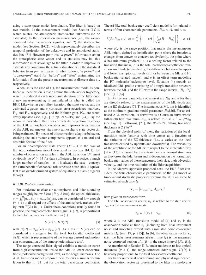
Fig. 3. Cross-examination of four classic ABL estimation methods (VCM,LGM, GM, and IPM). The black line represents the measured time-averagedrange-corrected lidar profile. The dark gray line corresponds to the first deriva-tive of the range-corrected lidar signal, ((dU(R))/(dR)), the dashed gray lineto the derivative of the logarithm, ((d lnU(R))/(dR)), and the dotted grayline to the second derivative, ((d2U(R))/(dR2)). The light gray dash-dottedline is the range-dependent variance of the lidar measurement set. Because allthe plots have different scales, they have been arbitrarily normalized so thatthey can be plotted on the same scale for visual purposes.

The NLSQ estimator operates in the range interval R =[R1, R2] while the EKF operates in the inner interval R =[R′

1, R′2] and in the outer intervals [R1, R

′1] and [R2, R

′2] [see

(10)–(13)]. The ratio between the lengths of the inner and full-range intervals is usually set between 0.6 and 0.8.

The classical methods studied are the threshold method(THM) [13], [16], [17], derivative methods (see, e.g., [18] and[33] for a review), and the centroid/variance method (VCM)[34]. The first two are based on the geometrical morphology ofthe backscatter lidar signal while the third one falls into the sta-tistical analysis class of methods. In the THM, a given thresholdis applied to the range-corrected profile to differentiate betweena high-level backscatter region and a low-level backscatterregion. The derivative methods presented are the gradientmethod (GM) [10], [26], the logarithmic gradient method(LGM) [35], and the inflection point method (IPM) [36]. TheGM and LGM seek for the range position corresponding tothe absolute minimum of either the first derivative or the firstderivative of the logarithm of the range-corrected signal. Thederivative of the logarithm enhances the aerosol contrast [33],but also, the noise contamination is amplified. The IPM methodcomputes the minimum of the second derivative to find theinflection points of the range-corrected lidar profile. Finally, theVCM computes the average ABL “centroid” height which isdefined as the lowest range position of a local maximum of thevariance profile [34].

In order to cross-examine the classical methods, Fig. 3shows a measured range-corrected profile at 1064 nm fromthe RSLab lidar system (black line) along with the computedfirst and second derivatives and the variance profile. The firstderivative (dark gray line) has been computed by averaging500 lidar vertical profiles in combination with a range-smoothing rectangular sliding window over the lidar signal. Thewindow length is 35 samples, and the raw-data spatial resolu-tion is 2.3 m/sample. The pulse repetition frequency is 20 Hz.This yields a temporal resolution of ΔtGM ∼ 25 s and a clean-data spatial resolution of ΔRGM ∼ 80 m in the determinationof the ABL height. The first derivative of the logarithm and

the second derivative have been computed by using the samesmoothing parameters as for the GM. To determine the varianceprofile, a larger range smoothing has been used (ΔRVCM ∼100 m), which leads to a slightly worse spatial resolution. Thetime resolution of the variance profile (light gray dash-dottedline) is ΔtVCM ∼ 190 s. Therefore, the VCM has a poorer timeresolution as compared with the derivative methods.

Range smoothing and time averaging are enough to ensuresufficient SNR (≥ 10) in the applicability of the classical meth-ods presented earlier, although they often give biased resultsand a reduced resolution [18], [33]. As a common trait, almostall methods lack, in some degree, the requirements to operatein an unattended real-time basis to monitor the ABL. Whereasstatistical methods like the VCM cannot follow the fast timescales of the lidar profiles, nonadaptive geometrical methodsdo not have the capability to assimilate past ABL estimates toenhance their ABL estimates with time.

A. High-SNR Case Study

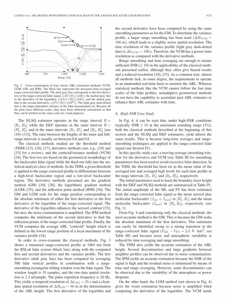
In Fig. 4, it can be seen that, under high-SNR conditions(typically SNR ≥ 10 at the maximum sounding range [31]),both the classical methods described at the beginning of thissection and the NLSQ and EKF estimators, yield almost thesame results. This is because long-time averages and range-smoothing techniques are applied to the range-corrected lidarsignal (see Section IV).

In this specific study case, a moving-average smoothing win-dow for the derivative and VCM (see Table III for smoothingparameters) has been used to avoid excessive false detection. Inthe THM, the threshold has been set as the mean value of theaveraged low and averaged high levels for each time profile inthe range intervals [R1, R

′1] and [R2, R

′2], respectively.

The initial parameters used to track the boundary layer heightwith the EKF and NLSQ methods are summarized in Table IV.The initial amplitude of the ML and FT has been estimatedfrom the range-corrected lidar signal as the mean aerosol plusmolecular backscatter (βaer + βmol) in [R′

1, R1] and the meanmolecular backscatter (βmol) in [R′

2, R2], respectively (seeFig. 1).

From Fig. 4 and considering only the classical methods, themost accurate method is the GM. This is because the GM seeksthe absolute minimum of the first derivative. This minimumcan easily be identified owing to a strong transition in therange-corrected lidar signal (VML − VFT = 2.5 V · km2; seeTable III) and because noise and atmospheric variability isreduced by time averaging and range smoothing.

The THM also yields the accurate estimation of the ABLheight. Several discontinuities and large gradients betweenneighbor profiles can be observed due to noise contamination.The IPM yields an accurate estimation because the SNR of thesignal is high and the residual noise is minimized by means oftime and range averaging. However, some discontinuities canbe observed due to the variability of the atmosphere or powerdropouts.

On the other hand, the LGM method (not shown in Fig. 4)gives the worst estimation because noise is amplified whencomputing the derivative of the logarithm. The VCM needs


Fig. 4. High-SNR case, ABL sunset (UPC, Campus Nord, Barcelona, on December 16, 2010). (a) Time–height plot of the range-corrected lidar signal for the1064-nm channel. ABL height retrieval by the following methods: (Red dots) GM, (green dots) LGM, (blue dots) THM, (white dots) IPM, (yellow dots) VCM,(black crosses) NLSQ estimator, and (magenta dots) EKF estimator. Lower and upper black lines represent R1 and R2, respectively, and lower and upper whitelines represent R′

1 and R′2. (b) Detail in the time interval from 19:40 to 19:43.

TABLE IIICLASSICAL-METHOD PARAMETERS USED FOR HIGH- AND

LOW-SNR CASE STUDIES (UNIT V · km2 REFERS

TO THE RANGE-CORRECTED SIGNAL, U(R))

higher time and range averages due to noise and shear-inducedturbulence, its performance being comparable to the LGM (thiseffect can also be observed in Fig. 3).

It should be noted that, because of the temporal windowlength (smoothing) required to compute the time averaging, allclassical methods can estimate the ABL height only up to theend of the time series minus the temporal smoothing lengthused (Δt1st in the case of the GM and LGM, Δt2nd in the caseof the IPM, and ΔtVCM in the case of VCM).

Regarding the NLSQ and the EKF, estimation runs until theend of the time series because no time or range smoothing isnecessary. Both methods give nearly identical results. There isonly a difference at the beginning of the time series because theABL height parameter Rbl was initialized with a considerablyhigher value than the real height just to show the robustness ofthe method under wrong parameters.

B. Low-SNR Case Study

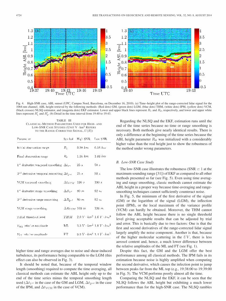
The low-SNR case illustrates the robustness (SNR � 1 at themaximum sounding range [31]) of EKF as compared to all othermethods presented so far (see Fig. 5). Even using time averag-ing and range smoothing, classic methods cannot estimate theABL height in a proper way because time-averaging and range-smoothing techniques cannot sufficiently counteract noise.

In Fig. 5, the minimum of the first derivative of the signal(GM) or the logarithm of the signal (LGM), the inflectionpoint (IPM), or the local maximum of the variance profile(VCM) can hardly be obtained. Moreover, the THM cannotfollow the ABL height because there is no single thresholdlevel giving acceptable results that can be adjusted by trialand error. This is basically due to two factors: One is that thefirst and second derivatives of the range-corrected lidar signallargely amplify the noise component. Another is that, becauseof the higher molecular scattering in the UV , there is lessaerosol content and, hence, a much lower difference betweenthe relative amplitudes of the ML and FT (see Fig. 1).

Despite this fact, the GM and the LGM offer the bestperformance among all classical methods. The IPM fails in itsestimation because noise is highly amplified when computingthe second derivative, which causes the infection point to jumpbetween peaks far from the ML top (e.g., 19:38:00 to 19:39:00in Fig. 5). The VCM performs poorly almost all the time.

Comparing the NLSQ and the EKF, it can be seen that theNLSQ follows the ABL height but exhibiting a much lowerperformance than for the high-SNR case. The NLSQ rambles


TABLE IVEKF AND NLSQ PARAMETERS

Fig. 5. Low-SNR case, ABL sunset (UPC, Campus Nord, Barcelona, on December 16, 2010). (a) Time–height plot of the range-corrected lidar signal for the355-nm channel. ABL height retrieval by the following methods: (Red dots) GM, (green dots) LGM, (blue dots) THM, (white dots) IPM, (yellow dots) VCM,(black crosses) NLSQ estimator, and (magenta dots) EKF estimator. Lower and upper black lines represent R1 and R2, respectively, and lower and upper whitelines represent R′

1 and R′2. (b) Detail in the time interval from 19:40 to 19:43.

between time-adjacent profiles in such a way that the ABLheight estimates become time discontinuous. On the other hand,the EKF follows the ABL height fairly consistently in instanceswhere all other methods evidence limitations. Thus, the EKFexhibits higher temporal and spatial resolution because, in orderto obtain consistent time-continuous estimates, the GM and theLGM require temporal and spatial smoothing as evidenced bypiecewise discontinuous estimates in Fig. 5 [e.g., time intervals19:37 to 19:38 in Fig. 5(a) or 19:40 to 19:41 in Fig. 5(b)]. In

addition, the GM and the LGM, when compared to the EKF,overestimate the ABL height with estimates starting to fall inthe FT zone [see Fig. 5(b)].

V. CONCLUSION

It has been shown that, in a scenario with a well-mixedlayer, without stratifications, and under high-SNR conditions,both classical and adaptive methods perform reasonably well


without unambiguous results (see Fig. 4). On the other hand,under low-SNR scenarios, ambiguities arise among these meth-ods (see Fig. 5). The EKF approach emerges as the mostsuitable method to track the temporal evolution of the ABLheight. NLSQ yields time-discontinuous ABL estimates that donot take benefit from past estimates and that fail to perform a“true” time tracking of the ABL height.

Thus, in low SNRs, derivative methods such as GM andLGM perform reasonably well only if the lidar signal is av-eraged in time and smoothed in range before these methodsare applied. Even in these conditions, the IPM performs poorlybecause the first and second derivatives of the range-correctedlidar signal largely amplify measurement noise. The TM, whichshares with the derivative methods using a geometrical ap-proach, also performs poorly because it is very difficult to seta physically consistent threshold to estimate the ABL height inthe erf -like zone; moreover, there is no unique solution. In allthese methods, if the difference between ML and FT averagelevels is small (as is usually the case in the UV ) or if the lidarsignal is too noisy, false peaks lead to the misestimation of theABL height.

The VCM uses a statistical approach that requires a largenumber of profiles to compute a statistically significant vari-ance (see Section I). In low-SNR conditions, the VCMis often misled due to noise fluctuations or shear-inducedturbulence.

The EKF approach presented is based on estimating fourtime-adaptive coefficients (see Section II) of an oversimplifiederf -like curve model representing the ABL transition. Fur-thermore, the filter is able to combine previous estimates inorder to improve the actual one, which permits to work withlow-SNR atmospheric scenes without excessively losing thetemporal resolution of the lidar instrument by a long pulseaveraging. This issue clearly outperforms the NLSQ estimates.These capabilities allow the EKF to avoid sudden changes ordropouts in the estimates of consecutive profiles, as it happenswith the NLSQ.

EKF and NLSQ methods perform better than the classicalmethods so far presented, particularly under low-SNR condi-tions. Under high-SNR conditions, both estimators reduce tothe same solution, as it can be shown theoretically that the EKFconverges to the NLSQ for SNR → ∞ (see Section II-C3).

Simulation tests of Section III have shown that the boundary-layer height, Rbl, and the transition amplitude, A, are the easiestparameters to estimate (higher sensitivity) while the EZ-scalingparameter, a, and the molecular-background parameter, c, arethe least sensitive ones in (4).

The actual implementation of the EKF method is limited torelatively clear atmosphere conditions and to the oversimplifiederf -like profile used to model the ML and EZ thickness. Furtherimplementations of the filter will take care of this limitation.

APPENDIX

NORMALIZATION OF THE RANGE-CORRECTED

LIDAR SIGNAL

The lidar signal of (1) can be written in expanded form as in(20), shown at the bottom of the page, where

K ′aer = Ke

−2∫ R0

0αaer(u)du (21)

and R0 is the end of the ABL (equivalently, the starting rangeof the FT containing only molecules, R′

2 in Fig. 1).Because the lidar system constant K is undetermined in

practice (or known with large errors) and the lidar signal iscorrupted with different background offsets of natural andinstrument origins, a molecular reference range (e.g., [R′

2, R2]in Fig. 1) in the FT is used to calibrate the lidar signal[37], [38].

In a molecular reference range, αmol(R) and βmol(R),the molecular extinction and backscatter profiles, respectively,are known from U.S. standard atmospheric and ground-level temperature and pressure conditions from radiosound-ing data.

Because the ABL transition model of (4) (see Fig. 1) isformulated in terms of the total backscatter coefficient, β(R),a normalization factor for (20) must be derived.

Assuming a ground-based backscatter lidar and consideringas molecular reference range the region R > R′

2 in Fig. 1, (20)fits βmol(R) when (20) is multiplied by a scaling factor

ζ =1

K ′aer

e2∫ R

0αmol(u)du. (22)

This yields the sought-after molecular normalized version ofU(R), Un(R). In expanded form

Un(R) =

{[βmol(R) + βaer(R)] e

2∫ R0

Rαaer(u)du, R ≤ R0

βmol(R), R > R0.(23)

At this point, it is interesting to see that, for R < R0 and

assuming low optical thickness (e2∫ R0

R � 1)

Un(R) �{βmol(R) + βaer(R), R ≤ R0

βmol(R), R > R0

(24)

which is in accordance to the model of (4) and Fig. 1.The observation vector, zk, is computed from the measured

lidar signals at each time tk as

zk = ζZk(R) (25)

where Zk(R) = Uk(R) + vk(R) is the discrete range-corrected measured lidar signal at time tk, with Uk(R) beingthe noiseless range-corrected backscatter power of (1), and vk

is the additive range-corrected instrumental noise.

U(R) =

⎧⎨⎩K [βmol(R) + βaer(R)] e

−2∫ R

0[αaer(u)+αmol(u)]du, if R ≤ R0

K ′aerβmol(R)e

−2∫ R

0αmol(u)du, if R > R0

(20)


ACKNOWLEDGMENT

This work was supported in part by the European Unionthrough the projects Initial Training in Atmospheric RemoteSensing (ITARS) under Grant 289923 and Aerosols, Clouds,and Trace Gases Research Infrastructure Network (ACTRIS)under Grant 262254 and in part by the Spanish Ministry ofEconomy and Competitivity (MEC) and European RegionalDevelopment (FEDER) funds through the project TEC2012-34575 and Complementary Action CGL2008-01330-E/CLI.The authors would like to thank the Spanish Ministry of ForeignAffairs and Cooperation (MAEC-AECID) and the EuropeanUnion/Initial Training in Atmospheric Remote Sensing for thepredoctoral fellowships of D. Lange and U. Saeed, respectively.The authors would also like to thank the Spanish Ministry ofScience and Innovation (MICINN) for the Granted BES-2007-17047 predoctoral fellowship of Dr. S. Tomás when at theRemote Sensing Laboratory (RSLab), Universitat Politècnicade Catalunya.

REFERENCES

[1] P. Seibert, F. Beyrich, S. Gryning, S. Joffre, A. Rasmussen, and P. Tercier,“Review and intercomparison of operational methods for the determina-tion of the mixing height,” Atmos. Environ., vol. 34, no. 7, pp. 1001–1027,2000.

[2] S. Emeis, K. Schäfer, and C. Münkel, “Surface-based remote sensing ofthe mixing-layer height: A review,” Meteorol. Zeitschr., vol. 17, no. 5,pp. 621–630, Oct. 2008.

[3] R. B. Stull, An Introduction to Boundary Layer Meteorology. New York,NY, USA: Springer-Verlag, 1988, ser. Atmospheric and OceanographicSciences Library, p. 670.

[4] V. A. Kovalev and W. E. Eichinger, Elastic Lidar: Theory, Practice, andAnalysis Methods. Hoboken, NJ, USA: Wiley, 2004, p. 615.

[5] B. A. Bodhaine, N. B. Wood, E. G. Dutton, and J. R. Slusser, “Rayleighoptical depth calculations,” J. Atmos. Ocean. Technol., vol. 16, no. 11,pp. 1854–1861, Nov. 1999.

[6] C. Pérez, S. Nickovic, J. M. Baldasano, M. Sicard, F. Rocadenbosch, andV. E. Cachorro, “A long Saharan dust event over the western Mediter-ranean: Lidar, Sun photometer observations, and regional dust model-ing,” J. Geophys. Res., vol. 111, no. D15, pp. D15214-1–D15214-16,Aug. 2006.

[7] P. Hägeli, D. G. Steyn, and K. B. Strawbridge, “Spatial and temporalvariability of mixed-layer depth and entrainment zone thickness,” Bound.-Lay. Meteorol., vol. 97, no. 1, pp. 47–71, Oct. 2000.

[8] S. Pal, A. Behrendt, and V. Wulfmeyer, “Elastic-backscatter-lidar-basedcharacterization of the convective boundary layer and investigationof related statistics,” Ann. Geophys., vol. 28, no. 3, pp. 825–847,Mar. 2010.

[9] M. Haeffelin, F. Angelini, Y. Morille, G. Martucci, C. D. O’Dowd,I. Xueref-Rémy, B. Wastine, S. Frey, and L. Sauvage, “Evaluation ofmixing depth retrievals from automatic profiling lidars and ceilometersin view of future integrated networks in Europe,” Bound.-Lay. Meteorol.,vol. 143, no. 1, pp. 49–75, Apr. 2011.

[10] R. M. Endlich, F. L. Ludwig, and E. E. Uthe, “An automatic method fordetermining the mixing depth from lidar observations,” Atmos. Environ.,vol. 13, no. 7, pp. 1051–1056, 1979.

[11] A. Lammert and J. Bösenberg, “Determination of the convective boundarylayer height with laser remote sensing,” Bound.-Lay. Meteorol., vol. 119,no. 1, pp. 159–170, Apr. 2005.

[12] S. Emeis, K. Schäfer, and C. Münkel, “Observation of the structure of theurban boundary layer with different ceilometers and validation by RASSdata,” Meteorol. Zeitschr., vol. 18, no. 2, pp. 149–154, May 2009.

[13] S. H. Melfi, J. D. Spinhirne, S. H. Chou, and S. P. Palm, “Lidar obser-vation of vertically organized convection in the planetary boundary layerover the ocean,” J. Clim. Appl. Meteorol., vol. 24, no. 8, pp. 806–821,Aug. 1985.

[14] K. E. Kunkel, E. W. Eloranta, and S. T. Shipley, “Lidar observations of theconvective boundary layer,” J. Appl. Meteorol., vol. 10, no. 12, pp. 1306–1311, Dec. 1977.

[15] A. Piironen and E. W. Eloranta, “Convective boundary layer mean depths,cloud base altitudes, cloud top altitudes, cloud coverages, and cloudshadows obtained from Volume Imaging Lidar data,” J. Geophys. Res.,vol. 100, no. 12, pp. 25 569–25 576, Dec. 1995.

[16] R. Boers and E. W. Eloranta, “Lidar measurements of the atmosphericentertainment zone and the potential temperature jump across the top ofthe mixed layer,” Bound.-Lay. Meteorol., vol. 34, no. 4, pp. 357–375,Mar. 2006.

[17] E. Batchvarova, D. G. Steyn, X. Cai, S.-E. Gryning, and M. Baldi, “Mod-elling the internal boundary layer in the Lower Fraser Valley,” in Proc.EURSAP Workshop Determination Mixing Height-Current Progr. Prob.,1997, vol. Risø-R-997(EN), pp. 141–144.

[18] M. Sicard, C. Pérez, F. Rocadenbosch, J. M. Baldasano, andD. García-Vizcaino, “Mixed-layer depth determination in the Barcelonacoastal area from regular lidar measurements: Methods, results and limi-tations,” Bound.-Lay. Meteorol., vol. 119, no. 1, pp. 135–157, Apr. 2006.

[19] R. G. Brown and P. Y. C. Hwang, Introduction to Random Signals andApplied Kalman Filtering. New York, NY, USA: Wiley, 1982.

[20] S. Tomás, F. Rocadenbosch, and M. Sicard, “Atmospheric boundary-layerheight estimation by adaptive Kalman filtering of lidar data,” in Proc.SPIE Remote Sens. Clouds Atmos. VIII, Toulouse, France, Sep. 21–23,2010, vol. 7827, pp. 782704-1–782704-10.

[21] D. G. Steyn, M. Baldi, and R. M. Hoff, “The detection of mixed layerdepth and entrainment zone thickness from lidar backscatter profiles,” J.Atmos. Ocean. Technol., vol. 16, no. 7, pp. 953–959, Jul. 1999.

[22] T. M. Mok and C. Z. Rudowicz, “A lidar study of the atmospheric en-trainment zone and mixed layer over Hong Kong,” Atmos. Res., vol. 69,no. 3/4, pp. 147–163, Jan.–Mar. 2004.

[23] F. Rocadenbosch, G. Vázquez, and A. Comerón, “Adaptive filter solutionfor processing lidar returns: Optical parameter estimation,” Appl. Opt.,vol. 37, no. 30, pp. 7019–7034, Oct. 1998.

[24] F. Rocadenbosch, C. Soriano, A. Comerón, and J. M. Baldasano, “Lidarinversion of atmospheric backscatter and extinction-to-backscatter ratiosby use of a Kalman filter,” Appl. Opt., vol. 38, no. 15, pp. 3175–3180,May 1999.

[25] A. Mukherjee, P. Adhikaria, P. K. Nandia, P. Palb, and J. Das, “Estimationof atmospheric boundary layer using Kalman filter technique,” SignalProcess., vol. 82, no. 11, pp. 1763–1771, Nov. 2002.

[26] C. Flamant, J. Pelon, P. H. Flamant, and P. Durand, “Lidar determinationof the entrainment zone thickness at the top of the unstable marine atmo-spheric boundary-layer,” Bound.-Lay. Meteorol., vol. 83, no. 2, pp. 247–284, May 1997.

[27] M. N. M. Reba, F. Rocadenbosch, and M. Sicard, “A straightforwardsignal-to-noise ratio estimator for elastic/Raman lidar signals,” in Proc.SPIE Remote Sens. Clouds Atmos. XI, Stockholm, Sweden, Sep. 11–14,2006, vol. 6362, pp. 626223-1–626223-12.

[28] M. N. M. Reba, F. Rocadenbosch, M. Sicard, C. Muñoz, and S. Tomás,“Piece-wise variance method for signal-to-noise ratio estimation inelastic/Raman lidar signals,” in Proc. IEEE IGARSS, Barcelona, Spain,Jul. 23–28, 2007, pp. 3158–3161.

[29] J. J. Moré, “The Levenberg-Marquardt algorithm: Implementation andtheory,” in Numerical Analysis. Lecture Notes in Mathematics. Berlin,Germany: Springer-Verlag, 1977, pp. 105–116.

[30] F. Rocadenbosch, M. Sicard, A. Comerón, and M. N. M. Reba, “Compar-ison between the Kalman and the non-linear least-squares estimators inlow signal-to-noise ratio lidar inversion,” in Proc. IEEE IGARSS, Boston,MA, USA, Jul. 6–11, 2008, vol. 3, pp. III-1083–III-1086.

[31] D. Kumar, D. Lange, F. Rocadenbosch, S. Tomás, M. Sicard,C. Muñoz, and A. Comerón, “Power budget and performance assessmentfor the RSLAB multispectral elastic/Raman lidar system,” in Proc. IEEEIGARSS, Jul. 22–27, 2012, pp. 4703–4706.

[32] R. T. H. Collis and P. B. Russell, “Lidar measurement of particles andgases by elastic backscattering and differential absorption,” in Laser Mon-itoring of the Atmosphere, E. D. Hinkley, Ed. New York, NY, USA:Springer-Verlag, 1976.

[33] G. Martucci, M. K. Srivastava, V. Mitev, R. Matthey, M. Froud, andH. Richner, “Comparison of lidar methods to determine the aerosol mixedlayer top,” in Proc. SPIE Remote Sens. Clouds Atmos. VIII, Maspalomas,Spain, Sep. 13–15, 2004, vol. 5235, pp. 447–456.

[34] W. P. Hooper and E. W. Eloranta, “Lidar measurements of wind in theplanetary boundary layer: The method, accuracy and results from jointmeasurements with radiosonde and kytoon,” J. Clim. Appl. Meteorol.,vol. 25, no. 7, pp. 990–100, Jul. 1986.

[35] C. Senff, J. Bösenberg, G. Peters, and T. S. Chaberl, “Remote sesing ofturbulent ozone fluxes and the ozone budget in the convective boundarylayer with DIAL and radar-RASS: A case study,” Contrib. Atmos. Phys.,vol. 69, no. 1, pp. 161–176, 1996.


[36] L. Menut, C. Flamant, J. Pelon, and P. H. Flamant, “Urban boundary-layerheight determination from lidar measurements over the Paris area,” Appl.Opt., vol. 38, no. 6, pp. 945–954, Feb. 1999.

[37] J. Bösenberg, R. Hoff, A. Ansmann, D. Müller, J. C. Antuna,D. Whitemann, N. Sugimoto, A. Apituley, M. Hardesty, J. Welton,E. Eloranta, Y. Arshinov, S. Kinne, and V. Freudenthaler, “Plan forthe implementation of the GAW Aerosol Lidar Observation Network(GALION),” World Meteorol. Org., Geneva, Switzerland, 1443, 2007,WMO Report.

[38] D. Lange, D. Kumar, and F. Rocadenbosch, “Backscattered signal leveland SNR validation methodology for tropospheric elastic lidars,” in Proc.IEEE IGARSS, Jul. 22–27, 2012, pp. 4707–4710.

Diego Lange received the B.S. degree in electronicsengineering from the San Simón University (UMSS),Cochabamba, Bolivia, in 2005 and the M.S. de-gree in electronics engineering from the UniversitatPolitècnica de Catalunya (UPC), Barcelona, Spain,in 2009. He is currently working toward the Ph.D.degree in the Remote Sensing Laboratory (RSLab),Department of Signal Theory and Communications,UPC, granted by the Spanish Ministry of ForeignAffairs and Cooperation (MAEC-AECID).

His research interests include multispectral lidarsignal processing, error-bound estimation, and adaptive lidar/radar inversion ofatmospheric optical parameters.

Jordi Tiana-Alsina was born in Barcelona,Catalunya, Spain, in 1981. He received the B.Sc.degree in physics from the Autonomous Universityof Barcelona, Barcelona, in 2005 and the Ph.D.degree from the Polytechnic University of Catalonia,Barcelona, in 2011. The focus of his researchwas on the analysis of the dynamical behavior ofsemiconductor lasers with optical feedback, as wellas the analysis of the synchronization of this kind ofsystems under different coupling architectures.

He is currently working on atmospheric lidar re-mote sensing systems at the Remote Sensing Laboratory (RSLab), Departmentof Signal Theory and Communications, Universitat Politècnica de Catalunya,Barcelona. His research interests include dynamics in semiconductor lasers aswell as signal processing applied to optical remote sensing technologies.

Umar Saeed received the B.E. degree in electronicsengineering from the National University of Sciencesand Technology, Karachi, Pakistan, in 2007 and theM.Sc. degree in communications engineering withspecialization in digital signal processing from theSchool of Electrical Engineering, Aalto University,Helsinki, Finland, in 2012. Currently, he is a Marie-Curie Early Stage Researcher in the framework ofthe Initial Training in Atmospheric Remote Sensingnetwork and is currently working toward the Ph.D.degree in the Remote Sensing Laboratory (RSLab),

Department of Signal Theory and Communications, Universitat Politècnica deCatalunya, Barcelona, Spain, granted by the European Union.

His research interests include the application of signal processing methods inactive optical and passive microwave atmospheric remote sensing and statisticaland adaptive processing.

Sergio Tomás received the M.S. and Ph.D. degreesin telecommunications engineering from the Uni-versitat Politècnica de Catalunya (UPC), Barcelona,Spain, in 2005 and 2011, respectively, and did hisundergraduate thesis at the Institute of Photonic Sci-ences (ICFO), Barcelona.

In 2012, he joined the Institute of Space Sciences(ICE-CSIC/IEEC) in Bellaterra, Spain, as a ResearchEngineer working in the detection of precipitationby means of polarimetric global navigation satel-lite system radio-occultations. His research interests

additionally include lidar remote sensing and related signal processing forwind monitoring and atmospheric boundary layer detection, and atmosphericturbulence.

Francesc Rocadenbosch (M’10) received the B.S.and Ph.D. degrees in telecommunications engineer-ing from the Universitat Politècnica de Catalunya(UPC), Barcelona, Spain, in 1991 and 1996, respec-tively, and the M.B.A. degree from the University ofBarcelona, Barcelona, Spain, in 2001.

From 1991 to 1992, he was with the University ofLas Palmas de Gran Canaria, Las Palmas de GranCanaria, Spain, working on microwave systems. In1993, he joined the Electromagnetics and PhotonicsEngineering (EEF) Group, Department of Signal

Theory and Communications (TSC), UPC, where he has been an AssociateProfessor since 1997 and a Joint Representative of the Remote Sensing Lab-oratory (RSLab), where he has been steering the development of the UPCactivities on multispectral elastic-Raman lidar (laser radar) since 1993. He isa reviewer of well-known international journals, such as Applied Optics, OpticsLetters, and Optical Engineering. His research interests include lidar remotesensing and cooperative remote-sensing sensors, related signal processing, and,more recently, its application to offshore wind farms (KIC-InnoEnergy strategicplan).

Dr. Rocadenbosch is an Associate Editor of the IEEE TRANSACTIONS

ON GEOSCIENCE AND REMOTE SENSING. He was the recipient of theSalvà i Campillo Best Research Project from the Catalan Association ofTelecommunication Engineers in 1998 as a member of the RSLab Lidar Group,the Telecommunications National Award in 2003 as a member of the EEFGroup, TSC Department, UPC, and the Best IEEE Reviewer Award from theTransactions on Geoscience and Remote Sensing in 2010.

atmospheric boundary layer height monitoring using a kalman filter and backscatter lidar returns

Documents