asymptotic analysis

An introduction to

asymptotic analysis

Simon J.A. Malham

Department of Mathematics, Heriot-Watt University

Contents

Chapter 1. Order notation 5

Chapter 2. Perturbation methods 92.1. Regular perturbation problems 92.2. Singular perturbation problems 15

Chapter 3. Asymptotic series 213.1. Asymptotic vs convergent series 213.2. Asymptotic expansions 253.3. Properties of asymptotic expansions 263.4. Asymptotic expansions of integrals 29

Chapter 4. Laplace integrals 314.1. Laplace’s method 324.2. Watson’s lemma 36

Chapter 5. Method of stationary phase 39

Chapter 6. Method of steepest descents 43

Bibliography 49

Appendix A. Notes 51A.1. Remainder theorem 51A.2. Taylor series for functions of more than one variable 51A.3. How to determine the expansion sequence 52A.4. How to find a suitable rescaling 52

Appendix B. Exam formula sheet 55

3

CHAPTER 1

Order notation

The symbols O, o and ∼, were first used by E. Landau and P. Du Bois-Reymond and are defined as follows. Suppose f(z) and g(z) are functions ofthe continuous complex variable z defined on some domain D ⊂ C and possesslimits as z → z0 in D. Then we define the following shorthand notation forthe relative properties of these functions in the limit z → z0.

Asymptotically bounded:

f(z) = O(g(z)) as z → z0 ,

means that: there exists constants K ≥ 0 and δ > 0 such that, for 0 <|z − z0| < δ,

|f(z)| ≤ K|g(z)| .

We say that f(z) is asymptotically bounded by g(z) in magnitude as z → z0,or more colloquially, and we say that f(z) is of ‘order big O’ of g(z). Henceprovided g(z) is not zero in a neighbourhood of z0, except possibly at z0, then

∣∣∣∣

f(z)

g(z)

∣∣∣∣

is bounded .

Asymptotically smaller:

f(z) = o(g(z)) as z → z0 ,

means that: for all ε > 0, there exists δ > 0 such that, for 0 < |z − z0| < δ,

|f(z)| ≤ ε|g(z)| .

Equivalently this means that, provided g(z) is not zero in a neighbourhood ofz0 except possibly at z0, then as z → z0:

f(z)

g(z)→ 0 .

We say that f(z) is asymptotically smaller than g(z), or more colloquially,f(z) is of ‘order little o’ of g(z), as z → z0.

5

6 1. ORDER NOTATION

Asymptotically equal:

f(z) ∼ g(z) as z → z0 ,

means that, provided g(z) is not zero in a neighbourhood of z0 except possiblyat z0, then as z → z0:

f(z)

g(z)→ 1 .

Equivalently this means that as z → z0:

f(z) = g(z) + o(g(z)) .

We say that f(z) asymptotically equivalent to g(z) in this limit, or morecolloquially, f(z) ‘goes like’ g(z) as z → z0.

Note that O-order is more informative than o-order about the behaviourof the function concerned as z → z0. For example, sin z = z + o(z2) as z → 0tells us that sin z − z → 0 faster than z2, however sin z = z + O(z3), tells usspecifically that sin z − z → 0 like z3.

Examples.

• f(t) = O(1) as t→ t0 means f(t) is bounded when t is close to t0.

• f(t) = o(1) ⇒ f(t) → 0 as t→ t0.

• If f(t) = 5t2 + t+ 3, then f(t) = o(t3), f(t) = O(t2) and f(t) ∼ 5t2

as t→ ∞; but f(t) ∼ 3 as t→ 0 and f(t) = o(1/t) as t→ ∞.

• As t→ ∞, t1000 = o(et), cos t = O(1).

• As t→ 0+, t2 = o(t), e−1/t = o(1), tan t = O(t), sin t ∼ t.

• As t→ 0, sin(1/t) = O(1), cos t ∼ 1 − 12 t

2.

Remarks.

(1) In the definitions above, the function g(z) is often called a gaugefunction because it is the function against which the behaviour off(z) is gauged.

(2) This notation is also easily adaptable to functions of a discrete vari-able such as sequences of real numbers (i.e. functions of the positiveinteger n). For example, if xn = 3n2 − 7n + 8, then xn = o(n3),xn = O(n2) and xn ∼ 3n2 as n→ ∞.

(3) Often the alternative notation f(z) � g(z) as z → z0 is used in placeof f(z) = o(g(z)) as z → z0.

1. ORDER NOTATION 7

−1 −0.5 0 0.5 10.8

0.9

1

1.1

1.2

1.3

1.4

1.5

1.6

1.7

1.8

t

tan(

t)/t

Graph of tan(t)/t

−1 −0.5 0 0.5 10.84

0.86

0.88

0.9

0.92

0.94

0.96

0.98

1

1.02

t

sin(t)

/t

Graph of sin(t)/t

Figure 1. The behaviour of the functions tan(t)/t andsin(t)/t near t = 0. These functions are undefined at t = 0;but both these functions approach the value 1 as t approaches0 from the left and the right.

CHAPTER 2

Perturbation methods

Usually in applied mathematics, though we can write down the equationsfor a model, we cannot always solve them, i.e. we cannot find an analyticalsolution in terms of known functions or tables. However an approximateanswer may be sufficient for our needs provided we know the size of the errorand we are willing to accept it. Typically the first recourse is to numericallysolve the system of equations on a computer to get an idea of how the solutionbehaves and responds to changes in parameter values. However it is oftendesirable to back-up our numerics with approximate analytical answers. Thisinvariably involves the use of perturbation methods which try to exploit thesmallness of an inherent parameter. Our model equations could be a system ofalgebraic and/or differential and/or integral equations, however here we willfocus on scalar algebraic equations as a simple natural setting to introducethe ideas and techniques we need to develop (see Hinch [5] for more details).

2.1. Regular perturbation problems

Example. Consider the following quadratic equation for x which involvesthe small parameter ε:

x2 + εx− 1 = 0 , (2.1)

where 0 < ε � 1. Of course, in this simple case we can solve the equationexactly so that

x = −12ε±

√

1 + 14ε

2 ,

and we can expand these two solutions about ε = 0 to obtain the binomialseries expansions

x =

{

+1 − 12ε+ 1

8ε2 − 1

128ε4 + O(ε6) ,

−1 − 12ε− 1

8ε2 + 1

128ε4 + O(ε6) .

(2.2)

Though these expansions converge for |ε| < 2, a more important property isthat low order truncations of these series are good approximations to the rootswhen ε is small, and maybe more efficiently evaluated (in terms of computertime) than the exact solution which involves square roots.

However for general equations we may not be able to solve for the solutionexactly and we will need to somehow derive analytical approximations whenε is small, from scratch. There are two main methods and we will explore thetechniques involved in both of them in terms of our simple example (2.1).

9

10 2. PERTURBATION METHODS

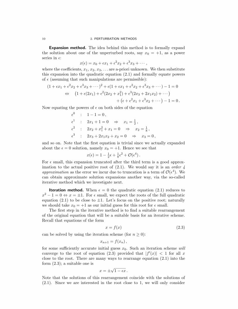
Expansion method. The idea behind this method is to formally expandthe solution about one of the unperturbed roots, say x0 = +1, as a powerseries in ε:

x(ε) = x0 + εx1 + ε2x2 + ε3x3 + · · · ,where the coefficients, x1, x2, x3, . . . are a-priori unknown. We then substitutethis expansion into the quadratic equation (2.1) and formally equate powersof ε (assuming that such manipulations are permissible):

(1 + εx1 + ε2x2 + ε3x3 + · · · )2 + ε(1 + εx1 + ε2x2 + ε3x3 + · · · ) − 1 = 0

⇔(1 + ε(2x1) + ε2(2x2 + x2

1) + ε3(2x3 + 2x1x2) + · · ·)

+(ε+ ε2x1 + ε3x2 + · · ·

)− 1 = 0 .

Now equating the powers of ε on both sides of the equation

ε0 : 1 − 1 = 0 ,

ε1 : 2x1 + 1 = 0 ⇒ x1 = 12 ,

ε2 : 2x2 + x21 + x1 = 0 ⇒ x2 = 1

8 ,

ε3 : 2x3 + 2x1x2 + x2 = 0 ⇒ x3 = 0 ,

and so on. Note that the first equation is trivial since we actually expandedabout the ε = 0 solution, namely x0 = +1. Hence we see that

x(ε) = 1 − 12ε+ 1

8ε2 + O(ε4) .

For ε small, this expansion truncated after the third term is a good approx-imation to the actual positive root of (2.1). We would say it is an order 4approximation as the error we incur due to truncation is a term of O(ε4). Wecan obtain approximate solution expansions another way, via the so-callediterative method which we investigate next.

Iteration method. When ε = 0 the quadratic equation (2.1) reduces tox2 − 1 = 0 ⇔ x = ±1. For ε small, we expect the roots of the full quadraticequation (2.1) to be close to ±1. Let’s focus on the positive root; naturallywe should take x0 = +1 as our initial guess for this root for ε small.

The first step in the iterative method is to find a suitable rearrangementof the original equation that will be a suitable basis for an iterative scheme.Recall that equations of the form

x = f(x) (2.3)

can be solved by using the iteration scheme (for n ≥ 0):

xn+1 = f(xn) ,

for some sufficiently accurate initial guess x0. Such an iteration scheme willconverge to the root of equation (2.3) provided that |f ′(x)| < 1 for all xclose to the root. There are many ways to rearrange equation (2.1) into theform (2.3); a suitable one is

x = ±√

1 − εx .

Note that the solutions of this rearrangement coincide with the solutions of(2.1). Since we are interested in the root close to 1, we will only consider

2.1. REGULAR PERTURBATION PROBLEMS 11

−2 −1.5 −1 −0.5 0 0.5 1 1.5 2−2

−1

0

1

2

3

4

x

f(x;ε

)Function f(x;ε)

−2 −1.5 −1 −0.5 0 0.5 1 1.5 20

0.5

1

1.5

2

roots

ε

Roots of f(x;ε)=0

ε=0.5ε=0

exactrootfour term asymptotic approx

Figure 1. In the top figure we see how the quadratic functionf(x; ε) = x2 + εx− 1 behaves while below we see how its rootsevolve, as ε is increased from 0. The dotted curves in the lowerfigure are the asymptotic approximations for the roots.


−2 −1.5 −1 −0.5 0 0.5 1 1.5 2−4

−2

0

2

4

x

f(x;ε

)Function f(x;ε)

−2 −1.5 −1 −0.5 0 0.5 1 1.5 20

0.1

0.2

0.3

0.4

0.5

0.6

0.7

roots

ε

Roots of f(x;ε)=0

ε=0.5ε=0

exactcuberootsthree term asymptotic approx

Figure 2. In the top figure we see how the cubic functionf(x; ε) = x3−x2− (1+ ε)x+1 behaves while below we see howits roots evolve, as ε is increased from 0. The dotted curvesin the lower figure are the asymptotic approximations for theroots close to 1.

2.1. REGULAR PERTURBATION PROBLEMS 13

the positive square root (we would take the negative square root if we wereinterested in approximating the root close to −1). Hence we identify f(x) ≡+√

1 − εx in this case and we have a rearrangement of the form (2.3). Alsonote that this is a sensible rearrangement as

∣∣f ′(x)

∣∣ =

∣∣∣∣

d

dx

(√1 − εx

)∣∣∣∣

=

∣∣∣∣

−ε/2√1 − εx

∣∣∣∣

≈ | − ε/2| .

In the last step we used that (1− εx)−1/2 ≈ 1 since x is near 1 and ε is small.In other words we see that close to the root

∣∣f ′(x)

∣∣ ≈ ε/2 ,

which is small when ε is small. Hence the iteration scheme

xn+1 =√

1 − εxn . (2.4)

will converge. We take x0 = 1 as our initial guess for the root.Computing the first approximation using (2.4), we get

x1 =√

1 − ε

=1 − 12ε− 1

8ε2 − 1

16ε3 − · · · ,

where in the last step we used the binomial expansion. Comparing this withthe expansion of the actual solution (2.2) we see that the terms of order ε2

are incorrect. To proceed we thus truncate the series after the second term sothat x1 = 1 − 1

2ε and iterate again:

x2 =√

1 − ε(1 − 1

2ε)

= 1 − 1

2ε(1 − 1

2ε)− 1

8ε2 (1 + · · · )2 + · · ·

= 1 − 12ε+ 1

8ε2 + · · · .

The term of order ε2 is now correct and we truncate x2 just after that termand iterate again:

x3 =√

1 − ε(1 − 1

2ε+ 18ε

2)

= 1 − 12ε(1 − 1

2ε+ 18ε

2)− 1

8ε2(1 − 1

2ε+ · · ·)2 − 1

16ε3 (1 + · · · )3 + · · ·

= 1 − 12ε+ 1

8ε2 + 0 · ε3 + · · · .

We begin to see that as we continue the iterative process, more work isrequired—and to ensure that the current highest term is correct we needto take a further iterate.

Remark. Note that the size of |f ′(x)| for x near the root indicates theorder of improvement to be expected from each iteration.


Example (non-integral powers). Find the first four terms in power seriesapproximations for the root(s) of

x3 − x2 − (1 + ε)x+ 1 = 0 , (2.5)

near x = 1, where ε is a small parameter. Let’s proceed as before using thetrial expansion method. First we note that at leading order (when ε = 0) wehave that

x30 − x2

0 − x0 + 1 = 0 ,

which by direct substitution, clearly has a root x0 = 1. If we assume the trialexpansion

x(ε) = x0 + εx1 + ε2x2 + ε3x3 + · · · ,and substitute this into (2.5), we soon run into problems when trying todetermine x1, x2, etc. . . by equating powers of ε—try it and see what happens!

However, if we go back and examine the equation (2.5) more carefully, werealize that the root x0 = 1 is rather special, in fact it is a double root since

x30 − x2

0 − x0 + 1 = (x0 − 1)2(x0 + 1) .

(The third and final root x0 = −1 is a single ordinary root.) Whenever wesee a double root, this should give us a warning that we should tread morecarefully.

Since the cubic x3 − x2 − (1 + ε)x + 1 has a double root at x = 1 whenε = 0, this means that it behaves locally quadratically near x = 1. Hence anorder ε change in x from x = 1 will produce and order ε2 change in the cubic

function (locally near x = 1). Equivalently, an order ε12 change in x locally

near x = 1, will produce an order ε change in the cubic polynomial. This

suggests that we instead should try a trial expansion in powers of ε12 :

x(ε) = x0 + ε12x1 + εx2 + ε

32x3 + · · · ,

Substituting this into the cubic polynomial (2.5) we see that

0 = x3 − x2 − (1 + ε)x+ 1

=(

1 + ε12x1 + εx2 + ε

32x3 + · · ·

)3−(

1 + ε12x1 + εx2 + ε

32x3 + · · ·

)2

− (1 + ε)(

1 + ε12x1 + εx2 + ε

32x3 + · · ·

)

+ 1

=(

1 + 3ε12x1 + ε(3x2

1 + 3x2) + ε32 (x3

1 + 6x1x2 + 3x3) + · · ·)

+(

1 + 2ε12x1 + ε(x2

1 + 2x2) + ε32 (2x1x2 + 2x3) + · · ·

)

−(

1 + ε12x1 + ε(1 + x2) + ε

32 (x1 + x3) + · · ·

)

+ 1 .

Hence equating coefficients of powers of ε:

ε0 : 1 − 1 − 1 + 1 = 0

ε12 : 3x1 − 2x1 − x1 = 0

ε : 3x21 + 3x2 − x2

1 − 2x2 − 1 − x2 = 0 ⇒ x1 = ± 1√2

ε32 : x3

1 + 6x1x2 + 3x3 − 2x1x2 − 2x3 − x1 − x3 = 0 ⇒ x2 = 18 .

2.2. SINGULAR PERTURBATION PROBLEMS 15

Hence

x(ε) ∼ 1 ± 1√2ε

12 + 1

8ε+ · · · .

Remark. If we were to try the iterative method, we might try to exploitthe significance of x = 1, and choose the following decomposition for anappropriate iterative scheme:

(x− 1)2(x+ 1) = εx ⇒ x = 1 ±√

εx

1 + x.

Example (non-integral powers). Find the first three terms in power seriesapproximations for the root(s) of

(1 − ε)x2 − 2x+ 1 = 0 , (2.6)

near x = 1, where ε is a small parameter.

Remark. Once we have realized that we need to pose a formal power

expansion in say powers of ε1n , we could equivalently set δ = ε

1n and expand

in integer powers of δ. At the very end we simply substitute back that δ = ε1n .

This approach is particularly convenient when you use either Maple1 to tryto solve such problems perturbatively.

Example (transcendental equation). Find the first three terms in thepower series approximation of the root of

ex = 1 + ε , (2.7)

where ε is a small parameter.

2.2. Singular perturbation problems

Example. Consider the following quadratic equation:

εx2 + x− 1 = 0 . (2.8)

The key term in this last equation that characterizes the number of solutionsis the first quadratic term εx2. This term is ‘knocked out’ when ε = 0. Inparticular we notice that when ε = 0 there is only one root to the equation,namely x = 1, whereas for ε 6= 0 there are two! Such cases, where the characterof the problem changes significantly from the case when 0 < ε� 1 to the casewhen ε = 0, we call singular perturbation problems. Problems that are notsingular are regular.

For the moment, consider the exact solutions to (2.8) which can be deter-mined using the quadratic equation formula,

x =1

2ε

(−1 ±

√1 + 4ε

).

1You can download a Maple worksheet from the course webpage which will help you toverify your algebra and check your homework answers.


Expanding these two solutions (for ε small):

x =

{

1 − ε+ 2ε2 − 5ε3 + · · · ,−1ε − 1 + ε− 2ε2 + 5ε3 + · · · .

We notice that as ε→ 0, the second singular root ‘disappears off to negativeinfinity’.

Iteration method. In order to retain the second solution to (2.8) as ε→ 0and keep track of its asymptotic behaviour, we must keep the term εx2 as asignificant main term in the equation. This means that x must be large. Notethat at leading order, the ‘−1’ term in the equation will therefore be negligiblecompared to the other two terms, i.e. we have

εx2 + x ≈ 0 ⇒ x ≈ −1

ε. (2.9)

This suggests the following sensible rearrangement of (2.8),

x = −1

ε+

1

εx,

and hence the iterative scheme

xn+1 = −1

ε+

1

εxn,

with

x0 = −1

ε.

Note that in this case

f(x) = −1

ε+

1

εx.

Hence

∣∣f ′(x)

∣∣ =

∣∣∣∣− 1

εx2

∣∣∣∣

=1

ε· 1

x2

≈ ε ,

when x ≈ −1/ε. Therefore, since ε is small, |f ′(x)| is small when x is closeto the root, and further, we expect an order ε improvement in accuracy witheach iteration. The first two steps in the iterative process reveals

x1 = − 1

ε− 1 ,

and

x2 = − 1

ε− 1

1 + ε

= − 1

ε− 1 + ε+ · · · .


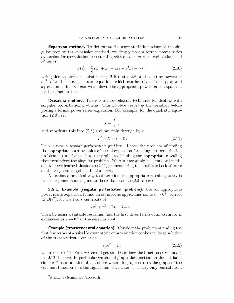
Expansion method. To determine the asymptotic behaviour of the sin-gular root by the expansion method, we simply pose a formal power seriesexpansion for the solution x(ε) starting with an ε−1 term instead of the usualε0 term:

x(ε) =1

εx−1 + x0 + εx1 + ε2x2 + · · · . (2.10)

Using this ansatz2, i.e. substituting (2.10) into (2.8) and equating powers ofε−1, ε0 and ε1 etc. generates equations which can be solved for x−1, x0 andx1 etc. and thus we can write down the appropriate power series expansionfor the singular root.

Rescaling method. There is a more elegant technique for dealing withsingular perturbation problems. This involves rescaling the variables beforeposing a formal power series expansion. For example, for the quadratic equa-tion (2.8), set

x =X

ε,

and substitute this into (2.8) and multiply through by ε,

X2 +X − ε = 0 . (2.11)

This is now a regular perturbation problem. Hence the problem of findingthe appropriate starting point of a trial expansion for a singular perturbationproblem is transformed into the problem of finding the appropriate rescalingthat regularizes the singular problem. We can now apply the standard meth-ods we have learned thusfar to (2.11), remembering to substitute back X = εxat the very end to get the final answer.

Note that a practical way to determine the appropriate rescaling to try isto use arguments analogous to those that lead to (2.9) above.

2.2.1. Example (singular perturbation problem). Use an appropriatepower series expansion to find an asymptotic approximation as ε→ 0+, correctto O(ε2), for the two small roots of

εx3 + x2 + 2x− 3 = 0 .

Then by using a suitable rescaling, find the first three terms of an asymptoticexpansion as ε→ 0+ of the singular root.

Example (transcendental equation). Consider the problem of finding thefirst few terms of a suitable asymptotic approximation to the real large solutionof the transcendental equation

ε xex = 1 , (2.12)

where 0 < ε� 1. First we should get an idea of how the functions ε xex and 1in (2.12) behave. In particular we should graph the function on the left-handside ε xex as a function of x and see where its graph crosses the graph of theconstant function 1 on the right-hand side. There is clearly only one solution,

2Ansatz is German for “approach”.


which will be positive, and also large when ε is small. In fact when 0 < ε� 1,then

xex =1

ε� 1 ⇒ x� 1 ,

confirming that we expect the root to be large. The question is how large, ormore precisely, exactly how does the root scale with ε?

Given that the dominant term in (2.12) is ex, taking the logarithm of bothsides of the equation (2.12) might clarify the scaling issue.

⇒ x+ lnx+ ln ε = 0

⇔ x = − ln ε− lnx

⇔ x = ln(

1ε

)− lnx ,

where in the last step we used that − lnA ≡ ln(

1A

). Now we see that when

0 < ε � 1 so that x � 1, then x � lnx and the root must lie near to ln(

1ε

),

i.e.

x ≈ ln(

1ε

).

This suggests the iterative scheme

xn+1 = ln(

1ε

)− lnxn ,

with x0 = ln(

1ε

). Note that in this case we can identify f(x) ≡ ln

(1ε

)− lnx,

and

∣∣f ′(x)

∣∣ =

∣∣∣∣

d

dx

(ln(

1ε

)− lnx

)∣∣∣∣

=

∣∣∣∣−1

x

∣∣∣∣

=1

|x|

≈ 1

ln(

1ε

) ,

when x is close to the root. Therefore |f ′(x)| is small since ε is small. Anothergood reason for choosing the iteration method here is that a natural expansionsequence is not at all obvious. The iteration scheme gives

x1 = ln(

1ε

)− ln ln

(1ε

).

Then

x2 = ln(

1ε

)− lnx1

= ln(

1ε

)− ln

(ln(

1ε

)− ln ln

(1ε

))

= ln(

1ε

)− ln

(

ln(

1ε

)

(

1 − ln ln(

1ε

)

ln(

1ε

)

))

= ln(

1ε

)− ln ln

(1ε

)− ln

(

1 − ln ln(

1ε

)

ln(

1ε

)

)

,


where in the last step we used that lnAB ≡ lnA + lnB. Hence, using theTaylor series expansion for ln(1−x), i.e. ln(1−x) ≈ −x, we see that as ε→ 0+,

x ∼ ln(

1ε

)− ln ln

(1ε

)+

ln ln(

1ε

)

ln(

1ε

) + · · · .

CHAPTER 3

Asymptotic series

3.1. Asymptotic vs convergent series

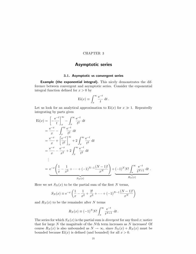
Example (the exponential integral). This nicely demonstrates the dif-ference between convergent and asymptotic series. Consider the exponentialintegral function defined for x > 0 by

Ei(x) ≡∫ ∞

x

e−t

tdt .

Let us look for an analytical approximation to Ei(x) for x � 1. Repeatedlyintegrating by parts gives

Ei(x) =

[

−e−t

t

]∞

x

−∫ ∞

x

e−t

t2dt

=e−x

x−∫ ∞

x

e−t

t2dt

=e−x

x+

[e−t

t2

]∞

x

+ 2

∫ ∞

x

e−t

t3dt

=e−x

x− e−x

x2+ 2

∫ ∞

x

e−t

t3dt

...

= e−x

(

1

x− 1

x2+ · · · + (−1)N−1 (N − 1)!

xN

)

︸︷︷︸

SN (x)

+ (−1)NN !

∫ ∞

x

e−t

tN+1dt

︸︷︷︸

RN (x)

.

Here we set SN (x) to be the partial sum of the first N terms,

SN (x) ≡ e−x(

1

x− 1

x2+

2!

x3+ · · · + (−1)N−1 (N − 1)!

xN

)

and RN (x) to be the remainder after N terms

RN (x) ≡ (−1)NN !

∫ ∞

x

e−t

tN+1dt .

The series for which SN (x) is the partial sum is divergent for any fixed x; noticethat for large N the magnitude of the Nth term increases as N increases! Ofcourse RN (x) is also unbounded as N → ∞, since SN (x) + RN (x) must bebounded because Ei(x) is defined (and bounded) for all x > 0.

21

22 3. ASYMPTOTIC SERIES

Suppose we consider N fixed and let x become large:

∣∣RN (x)

∣∣ =

∣∣∣∣(−1)NN !

∫ ∞

x

e−t

tN+1dt

∣∣∣∣

=∣∣(−1)N

∣∣N !

∫ ∞

x

e−t

tN+1dt

= N !

∫ ∞

x

e−t

tN+1dt

<N !

xN+1

∫ ∞

xe−t dt

=N !

xN+1e−x ,

which tends to zero very rapidly as x → ∞. Note that the ratio of RN (x) tothe last term in SN (x) is

∣∣∣∣

RN (x)

(N − 1)!e−xx−N

∣∣∣∣=

|RN (x)|(N − 1)!e−xx−N

<N !e−xx−(N+1)

(N − 1)!e−xx−N

=N

x, (3.1)

which also tends to zero as x→ ∞. Thus

Ei(x) = SN (x) + o(last term in SN (x)

)

as x → ∞. In particular, if x is sufficiently large and N fixed, SN (x) gives agood approximation to Ei(x); the accuracy of the approximation increases asx increases for N fixed. In fact, as we shall see, this means we can write

Ei(x) ∼ e−x(

1

x− 1

x2+

2!

x3+ · · ·

)

,

as x→ ∞.Note that for x sufficiently large, the terms in SN (x) will successively

decrease initially—for example 2!x−3 < x−2 for x large enough. However atsome value N = N∗(x), the terms in SN (x) for N > N∗ will start to increasesuccessively for a given x (however large) because the Nth term,

(−1)N−1e−x(N − 1)!

xN,

is unbounded as N → ∞.Hence for a given x, there is an optimal value N = N∗(x) for which the

greatest accuracy is obtained. Our estimate (3.1) suggests we should take N∗to be the largest integral part of the given x.

In practical terms, such an asymptotic expansion can be of more value thana slowly converging expansion. Asymptotic expansions which give divergentseries, can be remarkably accurate: for Ei(x) with x = 10; N∗ = 10, butS4(10) approximates Ei(10) with an error of less than 0.003%.

3.1. ASYMPTOTIC VS CONVERGENT SERIES 23

1 2 3 4 5 6 7 8 9 100

0.01

0.02

0.03

0.04

0.05

0.06

0.07

0.08

0.09

0.1

N

|(N−1

)! e−x

/xN

|

Magnitude of last term in SN

(x)

x=2x=2.5x=3

Figure 1. The behaviour of the magnitude of the last termin SN (x), i.e.

∣∣(−1)N−1(N − 1)!e−xx−N

∣∣, as a function of N

for different values of x.

Basic idea. Consider the following power series expansion about z = z0:

∞∑

n=0

an(z − z0)n . (3.2)

• Such a power series is convergent for |z − z0| < r, for some r ≥ 0,provided (see the Remainder Theorem)

RN (x) =∞∑

n=N+1

an(z − z0)n → 0 ,

as N → ∞ for each fixed z satisfying |z − z0| < r.

• A function f(z) has an asymptotic series expansion of the form (3.2)as z → z0, i.e.

f(z) ∼∞∑

n=0

an(z − z0)n , (3.3)

provided

RN (x) = o((z − z0)

N),

as z → z0, for each fixed N .


1 1.5 2 2.5 3 3.5 4 4.5 5

−0.02

0

0.02

0.04

0.06

0.08

0.1

0.12

x

Ei(x)

Exponential integral function

Ei(x)S

1(x)

S2(x)

S3(x)

S4(x)

1 1.5 2 2.5 3 3.5 4 4.5 5−5

−4

−3

−2

−1

0

1

x

log

10 |S

N(x

)−E

i(x)|

Logarithm of error in the asymptotic approximations

log10

|S1(x)−Ei(x)|

log10

|S2(x)−Ei(x)|

log10

|S3(x)−Ei(x)|

log10

|S4(x)−Ei(x)|

Figure 2. In the top figure we show the behaviour of the Ex-ponential Integral function Ei(x) and four successive asymp-totic approximations. The lower figure shows how the magni-tude of the difference between the four asymptotic approxima-tions and Ei(x) varies with x—i.e. the error in the approxima-tions is shown (on a semi-log scale).

3.2. ASYMPTOTIC EXPANSIONS 25

3.2. Asymptotic expansions

Definition. A sequence of gauge functions {φn(x)}, n = 1, 2, . . . is saidto form an asymptotic sequence as x→ x0 if, for all n,

φn+1(x) = o(φn(x)

),

as x→ x0.

Examples. (x− x0)n as x→ x0; x

−n as x→ ∞; (sinx)n as x→ 0.

Definition. If {φn(x)} is an asymptotic sequence of functions as x→ x0,we say that

∞∑

n=1

anφn(x)

where the an are constants, is an asymptotic expansion (or asymptotic ap-proximation) of f(x) as x→ x0 if for each N

f(x) =

N∑

n=1

anφn(x) + o(φN (x)

), (3.4)

as x → x0, i.e. the error is asymptotically smaller than the last term in theexpansion.

Remark. An equivalently property to (3.4) is

f(x) =N−1∑

n=1

anφn(x) + O(φN (x)

),

as x → x0 (which can be seen by using that the guage functions φn(x) forman asymptotic sequence).

Notation. We denote an asymptotic expansion by

f(x) ∼∞∑

n=1

anφn(x) ,

as x→ x0.

Definition. If the gauge functions form a power sequence, then the as-ymptotic expansion is called an asymptotic power series.

Examples. xn as x→ 0; (x− x0)n as x→ x0; x

−n as x→ ∞.


3.3. Properties of asymptotic expansions

Uniqueness. For a given asymptotic sequence {φn(x)}, the asymptoticexpansion of f(x) is unique; i.e. the an are uniquely determined as follows

a1 = limx→x0

f(x)

φ1(x);

a2 = limx→x0

f(x) − a1φ1(x)

φ2(x);

...

aN = limx→x0

f(x) −∑N−1n=1 anφn(x)

φN (x);

and so forth.

Non-uniqueness (for a given function). A given function f(x) may havemany different asymptotic expansions. For example as x→ 0,

tanx ∼ x+ 13x

3 + 215x

5 + · · ·∼ sinx+ 1

2(sinx)3 + 38(sinx)5 + · · · .

Subdominance. An asymptotic expansion may be the asymptotic expan-sion of more than one function. For example, if as x→ x0

f(x) ∼∞∑

n=0

an(x− x0)n ,

then also

f(x) + e− 1

(x−x0)2 ∼∞∑

n=0

an(x− x0)n ,

as x→ x0 because e− 1

(x−x0)2 = o((x− x0)

n)

as x→ x0 for all n.In fact,

∞∑

n=0

an(x− x0)n

is asymptotic as x→ x0 to any function which differs from f(x) by a functiong(x) so long as g(x) → 0 as x → x0 faster than all powers of x − x0. Such afunction g(x) is said to be subdominant to the asymptotic power series; theasymptotic power series of g(x) would be

g(x) ∼∞∑

n=0

0 · (x− x0)n .

Hence an asymptotic expansion is asymptotic to a whole class of functionsthat differ from each other by subdominant functions.

3.3. PROPERTIES OF ASYMPTOTIC EXPANSIONS 27

Example (subdominance: exponentially small errors). The function e−x

is subdominant to an asymptotic power series of the form

∞∑

n=0

anx−n

as x → +∞; and so if a function f(x) has such a asymptotic expansion, sodoes f(x) + e−x, i.e. f(x) has such an asymptotic power series expansion upto exponentially small errors.

Equating coefficients. If we write

∞∑

n=0

an · (x− x0)n ∼

∞∑

n=0

bn · (x− x0)n (3.5)

we mean that the class of functions to which

∞∑

n=0

an · (x− x0)n and

∞∑

n=0

bn · (x− x0)n

are asymptotic as x → x0, are the same. Further, uniqueness of asymptoticexpansions means that an = bn for all n, i.e. we may equate coefficients oflike powers of x− x0 in (3.5).

Arithmetical operations. Suppose as x→ x0,

f(x) ∼∞∑

n=0

anφn(x) and g(x) ∼∞∑

n=0

bnφn(x)

then as x→ x0,

αf(x) + βg(x) ∼∞∑

n=0

(an + bn) · φn(x) ,

where α and β are constants. Asymptotic expansions can also be multipliedand divided—perhaps based on an enlarged asymptotic sequence (which wewill need to be able to order). In particular for asymptotic power series, whenφn(x) = (x− x0)

n, these operations are straightforward:

f(x) · g(x) ∼∞∑

n=0

cn(x− x0)n ,

where cn =∑n

m=0 anbn−m and if b0 6= 0, d0 = a0/b0, then

f(x)

g(x)∼

∞∑

n=0

dn(x− x0)n ,

where dn =(

an −∑n−1

m=0 dmbn−m)

/b0.


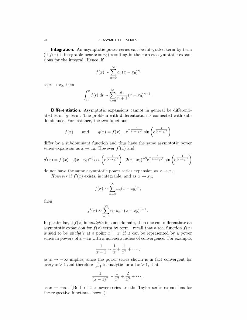
Integration. An asymptotic power series can be integrated term by term(if f(x) is integrable near x = x0) resulting in the correct asymptotic expan-sions for the integral. Hence, if

f(x) ∼∞∑

n=0

an(x− x0)n

as x→ x0, then∫ x

x0

f(t) dt ∼∞∑

n=0

ann+ 1

(x− x0)n+1 .

Differentiation. Asymptotic expansions cannot in general be differenti-ated term by term. The problem with differentiation is connected with sub-dominance. For instance, the two functions

f(x) and g(x) = f(x) + e− 1

(x−x0)2 sin

(

e1

(x−x0)2

)

differ by a subdominant function and thus have the same asymptotic powerseries expansion as x→ x0. However f ′(x) and

g′(x) = f ′(x)−2(x−x0)−3 cos

(

e1

(x−x0)2

)

+2(x−x0)−3e

− 1(x−x0)2 sin

(

e1

(x−x0)2

)

do not have the same asymptotic power series expansion as x→ x0.However if f ′(x) exists, is integrable, and as x→ x0,

f(x) ∼∞∑

n=0

an(x− x0)n ,

then

f ′(x) ∼∞∑

n=0

n · an · (x− x0)n−1 .

In particular, if f(x) is analytic in some domain, then one can differentiate anasymptotic expansion for f(x) term by term—recall that a real function f(x)is said to be analytic at a point x = x0 if it can be represented by a powerseries in powers of x−x0 with a non-zero radius of convergence. For example,

1

x− 1∼ 1

x+

1

x2+ · · · ,

as x → +∞ implies, since the power series shown is in fact convergent forevery x > 1 and therefore 1

x−1 is analytic for all x > 1, that

1

(x− 1)2∼ 1

x2+

2

x3+ · · · ,

as x → +∞. (Both of the power series are the Taylor series expansions forthe respective functions shown.)

3.4. ASYMPTOTIC EXPANSIONS OF INTEGRALS 29

3.4. Asymptotic expansions of integrals

Integral representations. When modelling many physical phenomena, itis often useful to know the asymptotic behaviour of integrals of the form

I(x) =

∫ b(x)

a(x)f(x, t) dt , (3.6)

as x → x0 (or more generally, the integral of a complex function along acontour). For example, many functions have integral representations:

• the error function,

Erf(x) ≡ 2√π

∫ x

0e−t

2dt;

• the incomplete gamma function (x > 0, a > 0),

γ(a, x) ≡∫ x

0e−t ta−1 dt .

Many other special functions such as the Bessel, Airy and hypergeometricfunctions have integral representations as they are solutions of various classesof differential equations. Also, if we use Laplace, Fourier or Hankel trans-formations to solve differential equations, we are often left with an integralrepresentation of the solution (eg. to determine an inverse Laplace trans-form we must evaluate a Bromwich contour integral). Two simple techniquesfor obtaining asymptotic expansions of integrals like (3.6) are demonstratedthrough the following two examples.

Example (Inserting an asymptotic expansion of the integrand). We canobtain an asymptotic expansion of the incomplete gamma function γ(a, x) asx → 0, by expanding the integrand in powers of t and integrating term byterm.

γ(a, x) =

∫ x

0

(

1 − t+t2

2!− t3

3!+ · · ·

)

ta−1 dt

=xa

a− xa+1

(a+ 1)+

xa+2

(a+ 2)2!− xa+3

(a+ 3)3!+ · · ·

= xa∞∑

n=0

(−1)nxn

(a+ n)n!,

which in fact converges for all x. However for large values of x, it convergesvery slowly which in practical terms is not very useful.

Example (Integrating by parts). For large x we can obtain an asymptoticexpansion of γ(a, x) as x→ +∞ as follows. Write

γ(a, x) =

∫ ∞

0e−t ta−1 dt

︸︷︷︸

Γ(a)

−∫ ∞

xe−t ta−1 dt

︸︷︷︸

Ei(1−a,x)

.


Recall that the (complete) gamma function Γ(a) is defined by

Γ(a) ≡∫ ∞

0e−t ta−1 dt .

And a generalization of the exponential integral above is labelled (x > 0)

Ei(1 − a, x) ≡∫ ∞

xe−t ta−1 dt .

We now integrate Ei(1 − a, x) by parts successively:

Ei(1 − a, x) = e−xxa−1 + (a− 1)

∫ ∞

xe−t ta−2 dt

...

= e−x(xa−1 + (a− 1)xa−2 + · · · + (a− 1) · · · (a−N + 1)xa−N

)

+ (a− 1)(a− 2) · · · (a−N)

∫ ∞

xe−t ta−N−1 dt.

Note that for any fixed N > a− 1,∣∣∣∣

∫ ∞

xe−t ta−N−1 dt

∣∣∣∣≤∫ ∞

x

∣∣e−t ta−N−1

∣∣ dt

=

∫ ∞

xe−t ta−N−1 dt

≤ xa−N−1

∫ ∞

xe−t dt

= xa−N−1e−x

= o(xa−Ne−x)

as x→ +∞, and so the expansion for Ei(1−a, x) above is asymptotic. Hence

γ(a, x) ∼ Γ(a) − e−x xa(

1

x+a− 1

x2+

(a− 1)(a− 2)

x3+ · · ·

)

,

as x → +∞, although the series is divergent. Note further that if RN (x) isthe remainder after N terms (and with N > a− 1):

∣∣RN (x)

∣∣

∣∣e−x xa−N (a− 1) · · · (a−N + 1)

∣∣≤ e−x xa−N−1

∣∣(a− 1) · · · (a−N)

∣∣

e−x xa−N∣∣(a− 1) · · · (a−N + 1)

∣∣

=

∣∣a−N

∣∣

x.

Hence for a given x, only use the largest number of N (integer) terms in theasymptotic expansion such that x > |a−N |.

CHAPTER 4

Laplace integrals

A Laplace integral has the form

I(x) =

∫ b

af(t) exφ(t) dt (4.1)

where we assume x > 0. Typically x is a large parameter and we are interestedin the asymptotic behaviour of I(x) as x→ +∞. Note that we can write I(x)in the form

I(x) =1

x

∫ b

a

f(t)

φ′(t)· d

dt

(

exφ(t))

dt .

Integrating by parts gives

I(x) =

[1

x· f(t)

φ′(t)· exφ(t)

]b

a︸︷︷︸

boundary term

− 1

x

∫ b

a

d

dt

(f(t)

φ′(t)

)

· exφ(t) dt

︸︷︷︸

integral term

. (4.2)

If the integral term is asymptotically smaller than the boundary term, i.e.

integral term = o(boundary term)

as x→ +∞, then

I(x) ∼[

1

x· f(t)

φ′(t)· exφ(t)

]b

a

as x→ +∞, i.e.

I(x) ∼ 1

x· f(b)

φ′(b)· exφ(b) − 1

x· f(a)

φ′(a)· exφ(a) (4.3)

and we have a useful asymptotic approximation for I(x) as x → +∞. Ingeneral, this will in fact be the case, i.e. (4.3) is valid, if φ(t), φ′(t) and f(t)are continuous functions (possibly complex) and the following condition issatisfied:

φ′(t) 6= 0 for a ≤ t ≤ b and either f(a) 6= 0 or f(b) 6= 0 .

This ensures that the integral term in (4.2) is bounded and is asymptoticallysmaller than the boundary term. Further, we may also continue to integrateby parts to generate further terms in the asymptotic expansion of I(x); eachintegration by parts generates a new factor of 1/x.

31

32 4. LAPLACE INTEGRALS

4.1. Laplace’s method

We can see that for Laplace integrals, integration by parts may fail forexample, when φ′(t) has a zero somewhere in a ≤ t ≤ b. Laplace’s methodis a general technique that allows us to generate an asymptotic expansionfor Laplace integrals for large x (and in particular when integration by partsfails). Recall

I(x) =

∫ b

af(t) exφ(t) dt

where we now suppose f(t) and φ(t) are real, continuous functions.

Basic idea. If φ(t) has a global maximum at t = c with a ≤ c ≤ b and iff(c) 6= 0, then it is only the neighbourhood of t = c that contributes to thefull asymptotic expansion of I(x) as x→ +∞.

Procedure.Step 1. We may approximate I(x) by I(x; ε) where

I(x; ε) =

∫ c+ε

c−εf(t) exφ(t) dt, if a < c < b,

∫ a+ε

af(t) exφ(t) dt, if c = a,

∫ b

b−εf(t) exφ(t) dt, if c = b,

(4.4)

where ε > 0 is arbitrary, but sufficiently small to guarantee that each of thesubranges of integration indicated are contained in the interval [a, b]. Sucha step is valid if the asymptotic expansion of I(x; ε) as x → +∞ does notdepend on ε and is identical to the asymptotic expansion of I(x) as x→ +∞.Both of these results are in fact true since (eg. when a < c < b) the terms

∣∣∣∣

∫ c−ε

af(t) exφ(t) dt

∣∣∣∣+

∣∣∣∣

∫ b

c+εf(t) exφ(t) dt

∣∣∣∣

are subdominant to I(x) as x → +∞. This is because exφ(t) is exponentially

small compared to exφ(c) for a ≤ t ≤ c− ε and c+ ε ≤ t ≤ b. In other words,changing the limits of integration only introduces exponentially small errors(all this can be rigorously proved by integrating by parts). Hence we simplyreplace I(x) by the truncated integral I(x; ε).

Step 2. Now ε > 0 can be chosen small enough so that (now we’re confinedto the narrow region surrounding t = c) it is valid to replace φ(t) by the firstfew terms in its Taylor or asymptotic series expansion.

• If φ′(c) = 0 with a ≤ c ≤ b and φ′′(c) 6= 0, approximate φ(t) by

φ(t) ≈ φ(c) +1

2φ′′(c) · (t− c)2 ,

4.1. LAPLACE’S METHOD 33

and approximate f(t) by

f(t) ≈ f(c) 6= 0. (4.5)

• If c = a or c = b and φ′(c) 6= 0, approximate φ(t) by

φ(t) ≈ φ(c) + φ′(c) · (t− c) ,

and approximate f(t) by

f(t) ≈ f(c) 6= 0. (4.6)

Step 3. Having substituted the approximations for φ and f indicatedabove, we now extend the endpoints of integration to infinity, in order to eval-uate the resulting integrals (again this only introduces exponentially smallerrors).

• If φ′(c) = 0 with a < c < b, we must have φ′′(c) < 0 (t = c is amaximum) and so as x→ +∞,

I(x) ∼∫ c+ε

c−εf(c)ex(φ(c)+ 1

2φ′′(c)·(t−c)2) dt

∼ f(c)exφ(c)

∫ ∞

−∞ex·

φ′′(c)2

(t−c)2 dt

=

√2f(c)exφ(c)

√

−xφ′′(c)

∫ ∞

−∞e−s

2ds (4.7)

where in the last step we made the substitution

s = +

√

−x · φ′′(c)

2(t− c) .

Since (see the formula sheet in Appendix B)∫ ∞

−∞e−s

2ds =

√π ,

we get

I(x) ∼√

2πf(c)exφ(c)

√

−xφ′′(c), (4.8)

as x→ +∞.If φ′(c) = 0 and c = a or c = b, then the leading order behaviour

for I(x) is the same as that in (4.8) except multiplied by a factor12—when we extend the limits of integration, we only do so in onedirection, so that the integral in (4.7) only extends over a semi-infiniterange.


• If c = a and φ′(c) 6= 0, we must have φ′(c) < 0, and as x→ +∞,

I(x) ∼∫ a+ε

af(a)ex(φ(a)+φ′(a)·(t−a)) dt

∼ f(a)exφ(a)

∫ ∞

0ex·φ

′(a)·(t−a) dt

⇒ I(x) ∼ − f(a)exφ(a)

xφ′(a).

If c = b and φ′(c) 6= 0, we must have φ′(c) > 0, and a similarargument implies that as x→ +∞,

I(x) ∼ f(b)exφ(b)

xφ′(b).

Remarks.

(1) If φ(t) achieves its global maximum at several points in [a, b], decom-pose the integral I(x) into several intervals, each containing a singlemaximum. Perform the analysis above and compare the contribu-tions to the asymptotic behaviour of I(x) (which will be additive)from each subinterval. The final ordering of the asymptotic expan-sion will then depend on the behaviour of f(t) at the maximal valuesof φ(t).

(2) If the maximum is such that φ′(c) = φ′′(c) = · · · = φ(m−1)(c) = 0

and φ(m)(c) 6= 0 then use that φ(t) ≈ φ(c) + 1m!φ

(m)(c) · (t− c)m.

(3) In (4.5) and (4.6) above we assumed f(c) 6= 0—see the beginning ofthis section—the case when f(c) = 0 is more delicate and treated inmany books—see Bender & Orszag [2].

(4) We have only derived the leading order behaviour. It is also possibleto determine higher order terms, though the process is much moreinvolved—again see Bender & Orszag [2].

Example (Stirling’s formula). We shall try to find the leading order be-haviour of the (complete) Gamma function

Γ(x+ 1) ≡∫ ∞

0e−t tx dt ,

as x→ +∞. First note that we can write

Γ(x+ 1) =

∫ ∞

0e−t+x ln t dt .

Second we try to convert it more readily to the standard Laplace integralform by making the substitution t = xr (this really has the effect of creating

4.1. LAPLACE’S METHOD 35

0 1 2 3 4 5−4

−3.5

−3

−2.5

−2

−1.5

−1

−0.5

0

0.5

r

exp(

x(ln

(r)−r

))

x=1

0 1 2 3 4 50

0.02

0.04

0.06

0.08

0.1

0.12

0.14

r

exp(

x(ln

(r)−r

))

x=2

0 1 2 3 4 50

0.005

0.01

0.015

0.02

r

exp(

x(ln

(r)−r

))

x=4

0 1 2 3 4 50

0.5

1

1.5

2

2.5

3

3.5x 10

−4

r

exp(

x(ln

(r)−r

))

x=8

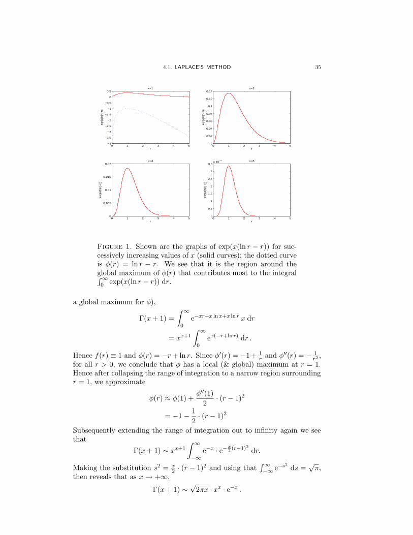
Figure 1. Shown are the graphs of exp(x(ln r − r)) for suc-cessively increasing values of x (solid curves); the dotted curveis φ(r) = ln r − r. We see that it is the region around theglobal maximum of φ(r) that contributes most to the integral∫∞0 exp(x(ln r − r)) dr.

a global maximum for φ),

Γ(x+ 1) =

∫ ∞

0e−xr+x lnx+x ln r x dr

= xx+1

∫ ∞

0ex(−r+ln r) dr .

Hence f(r) ≡ 1 and φ(r) = −r+ ln r. Since φ′(r) = −1 + 1r and φ′′(r) = − 1

r2,

for all r > 0, we conclude that φ has a local (& global) maximum at r = 1.Hence after collapsing the range of integration to a narrow region surroundingr = 1, we approximate

φ(r) ≈ φ(1) +φ′′(1)

2· (r − 1)2

= −1 − 1

2· (r − 1)2

Subsequently extending the range of integration out to infinity again we seethat

Γ(x+ 1) ∼ xx+1

∫ ∞

−∞e−x · e−x

2(r−1)2 dr.

Making the substitution s2 = x2 · (r − 1)2 and using that

∫∞−∞ e−s

2ds =

√π,

then reveals that as x→ +∞,

Γ(x+ 1) ∼√

2πx · xx · e−x .


0 0.5 1 1.5 2 2.5 3 3.5 4 4.5 510

−1

100

101

102

103

x

Γ(x+

1)

Accuracy of Stirlings formula

exactasymptotic

Figure 2. On a semi–log plot, we compare the exact valuesof Γ(x+ 1) with Stirling’s formula.

When x ∈ N, this is Stirling’s formula for the asymptotic behaviour of thefactorial function for large integers.

4.2. Watson’s lemma

Based on the ideas above, we can prove a more sophisticated result for asimpler Laplace integral.

Watson’s lemma. Consider the following example of a Laplace integral(for some b > 0)

I(x) ≡∫ b

0f(t) e−xt dt . (4.9)

Suppose f(t) is continuous on [0, b] and has the asymptotic expansion as t→0+ ,

f(t) ∼ tα∞∑

n=0

antβn . (4.10)

We assume that α > −1 and β > 0 so that the integral is bounded near t = 0;if b = ∞, we also require that f(t) = o(ect) as t → +∞ for some c > 0, toguarantee the integral is bounded for large t. Then as x→ +∞ ,

I(x) ∼∞∑

n=0

anΓ(α+ βn+ 1)

xα+βn+1. (4.11)

Proof. The basic idea is to use Laplace’s method and to take advantageof the fact that here we have the simple exponent φ(t) = −t in (4.9) (which hasa global maximum at the left end of the range of integration at t = 0). Thismeans that we can actually generate all the terms in the asymptotic power

4.2. WATSON’S LEMMA 37

series expansion of I(x) in (4.9) by plugging the asymptotic power series forf(t) in (4.10) into (4.9) and proceeding as before.

Step 1. Replace I(x) by I(x; ε) where

I(x; ε) =

∫ ε

0f(t)e−xt dt. (4.12)

This approximation only introduces exponentially small errors for any ε > 0.

Step 2. We can now choose ε > 0 small enough so that the first N termsin the asymptotic series for f(t) are a good approximation to f(t), i.e.

∣∣∣∣∣f(t) − tα

N∑

n=0

antβn

∣∣∣∣∣≤ K · tα+β(N+1), (4.13)

for 0 ≤ t ≤ ε and some constant K > 0. Substituting the first N terms in theseries for f(t) into (4.12) we see that, using (4.13),∣∣∣∣∣I(x; ε) −

N∑

n=0

an

∫ ε

0tα+βne−xt dt

∣∣∣∣∣=

∣∣∣∣∣

∫ ε

0

(

f(t) − tαN∑

n=0

antβn

)

e−xt dt

∣∣∣∣∣

≤∫ ε

0

∣∣∣∣∣f(t) − tα

N∑

n=0

antβn

∣∣∣∣∣e−xt dt

≤ K ·∫ ε

0tα+β(N+1)e−xt dt

≤ K ·∫ ∞

0tα+β(N+1)e−xt dt .

Hence using the identity∫ ∞

0tme−xt dt ≡ Γ(m+ 1)

xm+1(4.14)

we have just established that∣∣∣∣∣I(x; ε) −

N∑

n=0

an

∫ ε

0tα+βne−xt dt

∣∣∣∣∣≤ K · Γ(α+ β + βN + 1)

xα+β+βN+1.

Step 3. Extending the range of integration to [0,∞) and using the identity(4.14) again, we get that

I(x) =

N∑

n=0

an

∫ ∞

0tα+βne−xt dt+ o

(1

xα+βN+1

)

=N∑

n=0

anΓ(α+ βn+ 1)

xα+βn+1+ o

(1

xα+βN+1

)

,

as x → +∞. Since this is true for every N , we have proved (4.11) and thusthe Lemma. �


Remark. Essentially Watson’s lemma tells us that under the conditionsoutlined: if we substitute the asymptotic expansion (4.10) for f(t) into theintegral I(x) and extend the range of integration to 0 ≤ t ≤ ∞, then inte-grating term by term generates the correct asymptotic expansion for I(x) asx→ +∞.

Example. To apply Watson’s lemma to the modified Bessel function

K0(x) ≡∫ ∞

1(s2 − 1)−

12 e−xs ds ,

we first substitute s = t+ 1, so the lower endpoint of integration is t = 0:

K0(x) = e−x∫ ∞

0(t2 + 2t)−

12 e−xt dt .

For |t| < 2, the binomial theorem implies

(t2 + 2t)−12 = (2t)−

12(1 + t

2

)− 12

= (2t)−12

∞∑

n=0

(− t

2

)n · Γ(n+ 12)

n! Γ(12)

.

Watson’s lemma then immediately tells us that as x→ +∞

K0(x) ∼ e−x∫ ∞

0

∞∑

n=0

(2t)−12(− t

2

)n · Γ(n+ 12)

n! Γ(12)

e−xtdt

= e−x∞∑

n=0

Γ(n+ 12)

n! Γ(12)

(−1)n

2n+ 12

∫ ∞

0tn−

12 e−xtdt

= e−x∞∑

n=0

(−1)n ·(Γ(n+ 1

2))2

2n+ 12n! Γ(1

2)xn+ 12

.

Note. We can use Watson’s lemma to determine the leading order be-haviour (and higher orders) of more general Laplace integrals such as (4.1),as x→ +∞. Simply make the change of variables s = −φ(t) in (4.1) so that

I(x) = −∫ −φ(b)

−φ(a)F (s)e−xs , ds

where

F (s) = − f(φ−1(−s)

)

φ′(φ−1(−s)

) .

However, if t = φ−1(−s) is intricately multi-valued, then use the more directversion of Laplace’s method—for example if φ(t) has a global maximum att = c (for more details see Bender & Orszag [2]).

CHAPTER 5

Method of stationary phase

This method was originally developed by Stokes and Kelvin in the 19thcentury in their study of water waves. Consider the general Laplace integralin which φ(t) is pure imaginary, i.e. φ(t) = iψ(t) so that

I(x) =

∫ b

af(t) eixψ(t) dt,

where a, b, x, f(t) and ψ(t) are all real. In this case, I(x) is called the

generalized Fourier integral. Note that the term eixψ(t) is purely oscillatoryand so we cannot exploit the exponential decay of the integrand away from amaximum as was done in Laplace’s method and Watson’s lemma. However,if x is large, the integrand in I(x) oscillates rapidly and so we might expectapproximate cancellation of positive and negative contributions from adjacentintervals, leading to a small net contribution to the integral. In fact we havethe following result.

Riemann-Lebesgue lemma. If |f(t)| is integrable and ψ(t) is continu-ously differentiable over a ≤ t ≤ b, but ψ(t) is not constant over any subin-terval of a ≤ t ≤ b, then as x→ +∞,

I(x) =

∫ b

af(t) eixψ(t) dt→ 0 .

To obtain an asymptotic expansion of I(x) as x → +∞, we integrate byparts as before. This is valid provided the boundary terms are finite and theresulting integral exists; for example, provided that f(t)/ψ′(t) is smooth (inparticular bounded) over a ≤ t ≤ b and non-zero at either boundary, then

I(x) =

[f(t)

ixψ′(t)· eixψ(t)

]b

a︸︷︷︸

boundary term

− 1

ix

∫ b

a

d

dt

(f(t)

ψ′(t)

)

eixψ(t) dt

︸︷︷︸

integral term

.

The integral term is o(

1x

)as x→ +∞ by the Riemann-Lebesgue lemma and

so as x→ +∞,

I(x) ∼[f(t)

ixψ′(t)· eixψ(t)

]b

a

.

Integration by parts may fail if ψ(t) has a stationary point in the range ofintegration, i.e. ψ′(c) = 0 for some a ≤ c ≤ b.

Basic idea. If ψ′(c) = 0 for some a ≤ c ≤ b and ψ′(t) 6= 0 for all t 6= c in[a, b], then it is the neighbourhood of t = c that generates the leading orderasymptotic term in the full asymptotic expansion of I(x) as x→ +∞.

39

40 5. METHOD OF STATIONARY PHASE

Procedure.Step 1. For a small ε > 0 we decompose I(x) to I(x; ε) just like in (4.4)

for Laplace’s method. The remainder terms we neglect, for example in thecase when a < c < b, are

∫ c−ε

af(t) eixψ(t) dt+

∫ b

c+εf(t) eixψ(t) dt

and these vanish like 1/x as x→ +∞ because ψ(t) has no stationary points ineither interval and we can integrate by parts and apply the Riemann-Lebesguelemma.

Step 2. With ε small enough, to obtain the leading order behaviour wereplace ψ(t) and f(t) by the approximations

ψ(t) ≈ ψ(c) +ψ′′(c)

2!· (t− c)2

and

f(t) ≈ f(c) .

(This assumes ψ′′(c) 6= 0, otherwise we must consider higher order terms—seethe remarks below). Hence we get as x→ +∞,

I(x) ∼∫ c+ε

c−εf(c) e

ix·“

ψ(c)+ψ′′(c)

2!·(t−c)2

”

dt .

Step 3. We extend the range of integration to infinity in each direction—this again introduces terms which vanish like 1/x as x → +∞ and whichwill be asymptotically smaller terms that can be neglected. Then using thesubstitution

s = +

√

x · |ψ′′(c)|2

· (t− c) ,

(a change of variables due to Morse) yields

I(x) ∼ f(c) eixψ(c) ·√

2

x|ψ′′(c)| ·∫ ∞

−∞ei·sgn(ψ′′(c))·s2 ds , (5.1)

where

sgn(y) ≡{

+1 , if y > 0 ,

−1 , if y < 0 .

To evaluate the integral on the right, use that∫ ∞

−∞e±is2 ds =

√πe±iπ/4

so that eventually we get

I(x) ∼ f(c) · eixψ(c)+i·sgn(ψ′′(c))π/4 ·√

2π

x|ψ′′(c)| ,

as x→ +∞.

5. METHOD OF STATIONARY PHASE 41

Remarks.

(1) If c = a or c = b, the contribution from the integral, which is onlyover a semi-infinite interval, means that the asymptotic result abovemust be multiplied by a factor of 1

2 .

(2) If ψ(t) has many stationary points in [a, b], then we split up the in-tegral into intervals containing only one stationary point and dealwith each one independently (though their contributions are addi-tive). Again, the relative size of f(t) at the stationary points of ψ(t)will now be important.

(3) If the stationary point is such that ψ′(c) = ψ′′(c) = · · · = ψm−1(c) =

0 and ψm(c) 6= 0 then use that ψ(t) ≈ ψ(c)+ ψm(c)m! · (t− c)m instead.

In this case I(x) behaves like x−1/m as x→ +∞.

(4) Again, a very useful reference for more details is Bender & Orszag [2].

Example. To find the leading order asymptotic behaviour as x→ +∞ of

I(x) =

∫ 3

0t cosx

(13 t

3 − t)

dt ,

we first write the integral in the form

I(x) = Re

{∫ 3

0t eix

(13 t

3−t)

dt

}

so that we can identify f(t) ≡ t and ψ(t) = 13 t

3 − t. Hence ψ′(t) = t2 − 1 andψ′′(t) = 2t so that ψ has two stationary points, of which only the positive onelies in the range of integration at c = 1. Since ψ′′(t) = 2t > 0 for t ≥ 0, this isa local and global minimum. Hence truncating our interval of integration to asmall neighbourhood of c (this only introduces asymptotically smaller terms),we then make the approximations

ψ(t) ≈ ψ(c) +ψ′′(c)

2· (t− c)2 ,

and

f(t) ≈ f(c) .

Now we extend the endpoints of integration to infinity (again only introducingasymptotically smaller terms) so that as x→ +∞,

I(x) ∼ f(c) eixψ(c)

∫ ∞

−∞eix·ψ

′′(c)2

·(t−c)2 dt .

Making the substitution

s = +

√

x · ψ′′(c)

2· (t− c) ,

generates

I(x) ∼ f(c) eixψ(c) ·√

2

xψ′′(c)·∫ ∞

−∞eis2 ds .

42 5. METHOD OF STATIONARY PHASE

Since (see the formula sheet in Appendix B)∫ ∞

−∞eis2 ds =

√π eiπ/4 ,

we get

I(x) ∼ f(c) ei(xψ(c)+π/4) ·√

2π

xψ′′(c).

Now taking the real part of this and using that ψ(c) = −2/3, ψ ′′(c) = 2 andf(c) = 1 we get that as x→ +∞,

I(x) ∼√π

xcos

(π

4− 2x

3

)

.

0 0.5 1 1.5 2 2.5 3−3

−2

−1

0

1

2

3

t

t cos

(x(t

3 /3−

t))

x=10

0 0.5 1 1.5 2 2.5 3−3

−2

−1

0

1

2

3

t

t cos

(x(t

3 /3−

t))

x=50

0 0.5 1 1.5 2 2.5 3−3

−2

−1

0

1

2

3

t

t cos

(x(t

3 /3−

t))

x=100

0 0.5 1 1.5 2 2.5 3−3

−2

−1

0

1

2

3

t

t cos

(x(t

3 /3−

t))

x=200

Figure 1. This demonstrates why it is the region around thestationary point of the cubic 1

3 t3 − t that will contribute most

to the integral∫ 30 t cos

(x(

13 t

3 − t))

dt. Shown above are the

graphs of cos(x(

13 t

3 − t))

for successively increasing values of

x (solid curves); the dotted curve is the cubic 13 t

3 − t. We

see that away from the stationary point of 13 t

3 − t, the ar-

eas between the t-axis and cos(x(

13 t

3 − t))

approximately can-cel each other—which is rigorously embodied in the Riemann-Lebesgue Lemma.

CHAPTER 6

Method of steepest descents

This method originated with Riemann (1892). It is a general techniquefor finding the asymptotic behaviour of integrals of the form

I(λ) =

∫

Cf(z) eλh(z) dz ,

as λ → +∞, where C is a contour in the complex z-plane and f(z) & h(z)are analytic functions of z in some domain of the complex plane that containsC. The functions f(z) and h(z) need not be analytic in the whole of thecomplex plane C, in fact frequently in practice, they have isolated singularities,including branch points, the branch lines which must be carefully noted whenproceeding with the analysis below (for more details see Murray [9] and Bender& Orszag [2]).

Suppose h(z) = φ(z) + iψ(z), with φ(z) and ψ(z) both real valued, andthe contour C, which may be finite or infinite, joins the point z = a and z = b.Then, with ds = |dz|, we note that

|I(λ)| ≤∫ z=b

z=a

∣∣∣f(z) eλh(z)

∣∣∣ ds

≤∫ z=b

z=a|f(z)| eλφ(z) ds.

If∫ z=bz=a |f(z)| ds is bounded, then by Laplace’s method

|I(λ)| = O(eλφ) ,

ignoring multiplicative algebraic terms like λ−12 , λ−1, etc.. If |C| is bounded,

|I(λ)| ≤ |C| · maxC

{

|f(z)| eλφ(z)}

.

Hence we observe that the most important contribution to the asymptoticapproximation of |I(λ)| as λ → +∞ comes from the neighbourhood of themaximum of φ.

Basic idea. We can deform the contour C to a new contour C ′, usingCauchy’s theorem, at least in the domain of analyticity of f(z) and h(z).If f(z) has an isolated pole singularity for example, we can still deform thecontour C into another, which may involve crossing the singularity providedwe use the theory of residues appropriately (branch points/cuts need moredelicate care).

The reason for deforming C → C ′ is twofold:

43

44 6. METHOD OF STEEPEST DESCENTS

(1) we want to deform the path C so that φ drops off either side of itsmaximum at the fastest possible rate. In this way the largest valueof eλφ(z) as λ → +∞ will be concentrated in a small section of thecontour. This specific path through the point of the maximum ofeλφ(z) will be the contour of steepest descents. It is important to notehowever, that deforming the contour C in this way may alter its lengthand drastically change the variation of eλφ(z) in the neighbourhoodof its maximum when λ is large.

(2) we want to deform the path C so that h(z) has a constant imaginarypart, i.e. so that ψ is constant. The purpose of this is to eliminatethe necessity to consider rapid oscillations of the integrand when λis large. Such a contour is known as a constant–phase contour andwould mean that

I(λ) = eiλψ

∫

C′

f(z) eλφ(z) dz ,

which although z is complex, can be treated by Laplace’s methodas λ → +∞ because φ(z) is real. (Alternatively we could deformC so that φ is constant on it, and apply the method of stationaryphase. However, Laplace’s method is a much better approximationscheme as a full asymptotic expansion of a Laplace integral is de-termined by the integrand in an arbitrary small neighbourhood ofthe maximum of φ(z) on the contour; whereas the full asymptoticexpansion of a generalized Fourier integral depends on the behaviourof the integrand along the entire contour.)

So the question is: can we deform C → C ′ so that both these goals can besatisfied?

Recall. For a differentiable function f(x, y) of two variables, ∇f(x, y)points in the direction of the greatest rate of change of f at the point (x, y).The directional derivative in the direction of the unit vector n is ∂f/∂n =∇f ·n = the rate of f in the direction n. Hence on a two dimensional contourplot, ∇f is perpendicular to level contours of f , and the directional derivativein the direction parallel to the contour is zero.

Let h(z) be analytic in z, and for the moment, let us restrict ourselves to

regions of C where h′(z) 6= 0. We define a constant–phase contour of eλh(z),where λ > 0, as a contour on which ψ = Reh(z) is constant. We define a

steepest contour as one whose tangent is parallel to ∇|eλh(z)| = ∇eλφ(z), which

is parallel to ∇φ(z), i.e. a steepest contour is one on which eλh(z) is changingmost rapidly in z.

The important result here is, if h(z) is analytic with h′(z) 6= 0, then

constant–phase contours are steepest contours.

To prove this result, we note that since h(z) is analytic, then its real andimaginary parts satisfy the Cauchy-Riemann equations,

φx = ψy and φy = −ψx.

6. METHOD OF STEEPEST DESCENTS 45

Hence ∇φ · ∇ψ = 0; and thus ∇φ is perpendicular to ∇ψ provided h′(z) 6= 0.So the directional derivative of ψ in the direction of ∇φ is zero, which meansthat ψ is constant on contours whose tangents are parallel to ∇φ.

Note that where h′(z) 6= 0, there is a unique constant–phase/steepestcontour through that point.

Saddle points. When the contour of integration C is deformed into a con-stant phase contour C ′, we determine the leading order asymptotic behaviourof I(λ) from the behaviour of the integrand in the vicinity of the local max-ima of φ(z)—the local maxima may occur at an interior point of a contouror an endpoint. If the local maximum occurs at an interior point of the con-tour, then the directional derivative of φ along the contour vanishes, and theCauchy-Riemann equations imply that ∇φ = ∇ψ = 0. Hence h′(z) = 0 at aninterior maximum of φ on a constant–phase contour.

A point where h′(z) = 0 is called a saddle point ; at such points, two ormore level contours of ψ, and hence also steepest contours, may intersect. Notethat by the maximum modulus theorem, φ and ψ, cannot have a maximum (ora minimum) in the domain of analyticity of h(z) (where they are harmonic).

General procedure. First note that near the saddle point z0, we can ex-pand h(z) as a Taylor series

h(z) = h(z0) +1

2h′′(z0) · (z − z0)

2 + O((z − z0)

3).

We now deform the contour C (assuming in this case that the endpoints lie inthe valleys on either side of the saddle point) so that it lies along the steepestdescent path obtained by setting ψ(z) = ψ(z0). On this path, near z0,

φ(z) − φ(z0) = h(z) − h(z0) +1

2h′′(z0) · (z − z0)

2 < 0 ,

which is real (the constant imaginary parts cancel). Let us introduce the newreal variable τ by

h(z) − h(z0) = −τ2 , (6.1)

which determines z as a function of τ , i.e. z(τ). Hence

I(λ) = eλh(z0)∫ τb

τa

f(z(τ)) e−λτ2 · dz

dτdτ ,

where τa > 0 and τb > 0 correspond to the endpoints z = a and z = b ofthe original contour under the transformation (6.1). Laplace’s method thenimplies that as λ→ +∞,

I(λ) ∼ eλh(z0)

∫ +∞

−∞f(z(τ)) e−λτ

2 · dz

dτdτ . (6.2)

In this last expression, z(τ), and hence f(z(τ)) & dz/dτ , are obtained byinverting the transformation (6.1) on the steepest descent contour with ψ =ψ(z0): since

1

2h′′(z0) · (z − z0)

2 + O((z − z0)

3)

= −τ2 ,


we get

z − z0 =

√

−2

h′′(z0)· τ + O(τ2) . (6.3)

Now we require f(z(τ)) as a power series

f(z(τ)) = f(z0) + f ′(z0) · (z − z0) + · · ·

= f(z0) + f ′(z0) ·√

−2

h′′(z0)· τ + O(τ2) .

Substituting our expansions for f(z(τ)) and dz/dτ into (6.2), we get as λ →+∞,

I(λ) ∼ eλh(z0) · f(z0) ·√

−2

h′′(z0)

∫ +∞

−∞e−λτ

2dτ + · · · .

⇒ I(λ) = f(z0) ·√

−2π

λh′′(z0)· eλh(z0) + O

(

eλh(z0)

λ

)

.

Note. It is important in (6.3), since h′′(z0) is complex, to choose the

appropriate branch of√

−1h′′(z0) when z lies on the steepest descent path—

it must be chosen consistent with the direction of passage through the sta-tionary point. If there is more than one stationary point, then the relevantstationary point is the one which admits a possible deformation of the orig-inal contour into a path of steepest descents. If more than one stationarypoint is appropriate, then the one which gives the maximum φ is the rel-evant one. The method of steepest descents still applies even if the end-points of the original contour only lie in one valley (rather than in val-leys either side of the stationary point)—we still deform the contour to apath of steepest descents. If the stationary point is of order m − 1, i.e.h′(z0) = h′′(z0) = · · · = h(m−1)(z0) = 0 and h(m)(z0) 6= 0, then approximate

h(z) near z0 by h(z) = h(z0) + 1m!h

(m)(z0) · (z − z0)m instead, and proceed as

before.

Example. Consider the Gamma function, with a complex argument,

Γ(a+ 1) ≡∫ ∞

0e−t ta dt . (6.4)

The path of integration is along the real axis and a ∈ C, with |arg(a)| < π/2.We wish to find the asymptotic expansion of Γ(a + 1) as a → ∞ along someray. Since a ∈ C, the principal value of ta is taken with the branch line as thenegative real t-axis. To apply the method of steepest descents, we must firstexpress (6.4) in the appropriate form; consider the transformation

t = a(1 + z) , a = λeiα , λ > 0 , |α| < π

2,

6. METHOD OF STEEPEST DESCENTS 47

where now z is complex, and the contour C in the z-plane goes from z = −1(t = 0) to z = ∞ e−iα (t = +∞) with |α| < π/2:

Γ(a+ 1) = aa+1e−a∫ ∞ e−iα

−1eλ(e

iα(log(1+z)−z)) dz ,

where the principal value of the logarithm is taken with the branch line fromz = −1 along the negative real axis to z = ∞ eiπ. Hence we are now interestedin the asymptotic approximation as λ→ +∞ of

I(λ) =

∫

Ceλh(z) dz ,

where h(z) = eiα (log(1 + z) − z) and C is the contour already described.There is a single stationary point of h(z):

h′(z) = eiα

(1

1 + z− 1

)

= 0 ⇔ z = 0 .

Since h′′(0) = −1 6= 0, z = 0 is a stationary point of order 1. The path ofsteepest descents through z = 0 is

ψ = Im {h(z)} = Im {h(0)} = 0 ,

which, when expanding h(z) close to z = 0 is (setting z = reiθ, r > 0)approximately

Im

{

−eiα · 1

2z2

}

≈ 0 ⇒ r2 sin(2θ + α) ≈ 0 .

The paths of steepest descent and ascent near z = 0 are

θ = −1

2α with the continuation θ = π − 1

2α, (6.5)

θ = −1

2π − 1

2α with the continuation θ =

1

2π − 1

2α . (6.6)

Along (6.5) near z = 0,

φ = Re {h(z)} ≈ Re

{

−eiα · 1

2z2

}

= −1

2r2 cos(2θ + α) < 0 = φ(0)

and so (6.5) must be the path of steepest descents while (6.6) is the path ofsteepest ascents.

We now deform C to the steepest descents path in the vicinity of thestationary point, C ′, shown in the figure. Following the general procedure,introduce the new real variable τ by,

h(z) − h(0) = eiα (log(1 + z) − z) = −τ 2 .

Expanding the left-hand side in Taylor series near the stationary point z = 0gives

−eiα · 1

2z2 + · · · = −τ 2 ⇒ z(τ) = ±

√2 · e−iα/2 · τ + O(τ2) ,


where ±1 are the two branches of√

1. On the steepest descents path θ = −α/2near z = 0; we wish to have τ > 0. Since z = re−iα/2 on it, we must choosethe plus sign so

z(τ) = +√

2 · e−iα/2 · τ + O(τ2) .

Hence as λ→ +∞,

I(λ) =√

2 · e−iα/2

∫ +∞

−∞e−λτ

2dτ =

√

2π

λ· e−iα/2 =

√

2π

a.

And so

Γ(a+ 1) =√

2π · aa+ 12 e−a as a→ ∞ with |arg(a)| < π

2.

Bibliography

[1] Atkinson, K.E. An introduction to numerical analysis, John Wiley & Sons, 1978.[2] Bender, C.M. and Orszag, S.A. Advanced mathematical methods for scientists and en-

gineers, McGraw-Hill, 1978.[3] J.C. Burkill and H. Burkill, A second course in mathematical analysis, CUP, 1970.[4] Herbert, D. Lecture notes on asymptotic analysis, Imperial College, 1989.[5] Hinch, E.J. Perturbation methods, CUP, 1991.[6] Keener, J.P. Principles of applied mathematics: transformation and approximation,

Perseus Books, 2000.[7] Kevorkian, J. and Cole, J.D. Perturbation methods in applied mathematics, Applied

Mathematical Sciences 34, Springer–Verlag, 1981.[8] Lacey, A. Lecture notes on asymptotic analysis, Heriot-Watt, 2001.[9] Murray, J.D. Asymptotic analysis, Springer-Verlag, 1984.

[10] Marsden, J.E. and Ratiu, T.S. Introduction to mechanics and symmetry, Springer-Verlag, 1994.

[11] Rothe, K. Lecture notes on analysis, Imperial College, 1988.[12] Verhulst, F. Nonlinear differential equations and dynamical systems, Springer, 1996.

49

APPENDIX A

Notes

A.1. Remainder theorem

Theorem. (Remainders) Suppose f (n−1) is continuous in [a, a + h] anddifferentiable in (a, a+ h). Let Rn be defined by

f(a+ h) =n−1∑

m=0

f (m)(a)

m!· hm +Rn.

Then

(1) (with Legendre’s remainder) there exists θ ∈ (0, 1) such that

Rn =f (n)(a+ θh)

n!· hn;

(2) (with Cauchy’s remainder) there exists θ̃ ∈ (0, 1) such that

Rn = (1 − θ̃)n−1 f(n)(a+ θ̃h)

(n− 1)!· hn;

In particular, if we can prove that Rn → 0 as n→ ∞ (in either form above),then the Taylor expansion

∞∑

n=0

f (n)(a)

n!· hn

converges to f(a+ h).

A.2. Taylor series for functions of more than one variable

We can successively attempt to approximate f(x, y) near (x, y) = (a, b)by a tangent plane, quadratic surface, cubic surface, etc. . . , to generate theTaylor series expansion for f(x, y):

f(x, y) = f(a, b) + fx(a, b)(x− a) + fy(a, b)(y − b) (A.1)

+1

2!

(

fxx(a, b)(x− a)2

+ 2fx,y(a, b)(x− a)(y − b)

+ fyy(a, b)(y − b)2)

+ · · · .

Note that we can also derive the above series by expanding

F (t) = f(a+ ht, b+ kt) (A.2)

51

52 A. NOTES

in a Taylor series in the single independent variable t, about t = 0, withh = x− a, k = y − b, and evaluating at t = 1:

F (1) = F (0) + F ′(0) +1

2!F ′′(0) + · · · . (A.3)

Now using that F (t) is given by (A.2) in (A.3), we can generate (A.1).

A.3. How to determine the expansion sequence

Example. Consider the perturbation problem

(1 − ε)x2 − 2x+ 1 = 0 , (A.4)

for small ε. When ε = 0 this quadratic equation has a double root

x0 = 1 .

For small ε 6= 0 the quadratic equation (A.4) will have two distinct roots, bothclose to 1. To determine the appropriate expansion for both roots, we pose ageneral expansion of the form

x(ε) = 1 + δ1(ε)x1 + δ2(ε)x2 + · · · , (A.5)

where we require that

1 � δ1(ε) � δ2(ε) � · · · , (A.6)

and that x1, x2, . . . are strictly order unity as ε→ 0 (this means that they areO(1), but not asymptotically small as ε→ 0).

The idea is then to substitute (A.5) into (A.4) and, after cancelling off anyobvious leading terms and noting the asymptotic relations (A.6) and |ε| � 1,to consider the three possible leading order balances: δ2

1 � ε, δ21 = ε andδ21 � ε. For more details see Hinch [5].

A.4. How to find a suitable rescaling

For some singular perturbation problems it is difficult to guess what theappropriate rescaling should be a-priori. In this case, pose a general rescalingfactor δ(ε):

x = δX , (A.7)

where we will insist that X is strictly of order unity as ε→ 0. Then substitutethe rescaling (A.7) into the singular perturbation problem at hand, and ex-amine the balances within the rescaled problem for δ of different magnitudes.

Example. Consider the singular perturbation problem

εx3 + x2 − 1 = 0 , (A.8)

for small ε. In the limit as ε → 0, one of the roots is knocked out while theother two remaining roots are

x0 = ±1 .

For small ε 6= 0 the cubic equation will have two regular roots close to ±1;approximate expansions for these roots in terms of powers of ε can be found

A.4. HOW TO FIND A SUITABLE RESCALING 53

in the usual way. To determine the appropriate expansion for the remainingsingular root we substitute the rescaling (A.7) into (A.8) to get

εδ3X3 + δ2X2 − 1 = 0 . (A.9)

It is quite clear in this simple example that the appropriate rescaling thatregularizes the problem is δ = 1/ε—we could also use the argument that weexpect the singular root to be large for small ε and hence at leading order wehave

εx3 + x2 ≈ 0 ⇒ x ≈ −1

ε.

However let’s suppose that we did not see this straight away and try to deduceit by considering δ of different magnitudes and examining the relative size ofthe terms in the left-hand side of (A.9) as follows.

• If δ � 1, thenεδ3X3︸︷︷︸

o(1)

+ δ2X2︸︷︷︸

o(1)

−1 .

where by o(1) we of course mean asymptotically small (� 1). Withthis rescaling the left-hand side of (A.9) clearly cannot balance zeroon the right-hand side and so this rescaling is unacceptable.

• If δ = 1, thenεδ3X3︸︷︷︸

o(1)

+δ2X2 − 1 .

We can balance zero (on the right-hand side) in this case and thisrescaling corresponds to the trivial one we would make for the tworegular roots, i.e. we get that X = ±1 + o(1).

• If 1 � δ � ε−1, then (after dividing through by δ2)

εδX3︸︷︷︸

o(1)

+X2 − 1/δ2︸︷︷︸

o(1)

.

For this rescaling we cannot balance zero on the right-hand side unlessX = 0+o(1), but this violates our assumption that X is strictly orderunity. Hence this rescaling in unacceptable.

• If δ = ε−1, then (after dividing through by εδ3)

X3 +X2 − 1/εδ3

︸︷︷︸

o(1)

.

This can balance zero on the right-hand side if

X = −1 + o(1) ,

orX = 0 + o(1) .

The first solution must correspond to the singular root, whilst thesecond violates our assumption that X is strictly order unity.

54 A. NOTES

• If ε−1 � δ, then (after dividing through by εδ3)

X3 + 1εδ X

2

︸︷︷︸

o(1)

− 1/εδ3

︸︷︷︸

o(1)

.

This cannot balance zero on the right-hand side unless X = 0+o(1),but this violates our assumption that X is strictly order unity. Hencethis rescaling in unacceptable.

Hence δ = 1 is the suitable rescaling for the regular root and δ = ε−1 isthe suitable rescaling for investigating the singular root.

APPENDIX B

Exam formula sheet

Power series.

ex = 1 + x+1

2!x2 +

1

3!x3 + · · · for all x

sinx = x− 1

3!x3 +

1

5!x5 − 1

7!x7 ± · · · for all x

cosx = 1 − 1

2!x2 +

1

4!x4 − 1

6!x6 ± · · · for all x

sinhx = x+1

3!x3 +

1

5!x5 +

1

7!x7 + · · · for all x

coshx = 1 +1

2!x2 +

1

4!x4 +

1

6!x6 + · · · for all x

(a+ x)k = ak + kak−1x+k(k − 1)

2!ak−2x2 + · · · for |x| < a

log(1 + x) = x− 1

2x2 +

1

3x3 − 1

4x4 ± · · · for |x| < 1

Integration by parts formula.∫ b

au(t)v′(t) dt =

[u(t)v(t)

]t=b

t=a−∫ b

au′(t)v(t) dt .

55

56 B. EXAM FORMULA SHEET

Perturbation expansions.

x(ε) = x0 + x1ε+ x2ε2 + x3ε

3 + x4ε4 + O(ε5)

(x(ε)

)2= x2

0 + 2x0x1ε+ (x21 + 2x0x2)ε

2 + (2x1x2 + 2x0x3)ε3

+ (x22 + 2x1x3 + 2x0x4)ε

4 + O(ε5)

(x(ε)

)3= x3

0 + 3x20x1ε+ 3(x0x

21 + x2

0x2)ε2 + (x3

1 + 6x0x1x2 + 3x20x3)ε

3

+ 3(x21x2 + 2x0x1x3 + x0x

22 + x2

0x4)ε4 + O(ε5)

(x(ε)

)4= x4

0 + 4x30x1ε+ 2(3x2

0x21 + 2x3

0x2)ε2 + 4(x0x

31 + 3x2

0x1x2 + x30x3)ε

3

+ (x41 + 12x0x

21x2 + 6x2

0x22 + 12x2

0x1x3 + 4x30x4)ε

4 + O(ε5)

Definite integrals.∫ ∞

0sn−1 e−s ds = n! for n = 0, 1, 2, 3, . . .

∫ ∞

0sα−1 e−s ds = Γ(α) for α > 0

∫ ∞

−∞e−s

2ds =

√π

∫ ∞

−∞s2 e−s

2ds =

√π

2

∫ ∞

−∞e±is2 ds =

√π e±iπ/4

asymptotic analysis

Documents

sin z z

limit z z0

z oz3

z oz2

neighbourhood of z0

ft 5t2as t

possiblyat z0

5t2 t