Asymmetric information and economies-of-scale in

service contracting

Mustafa Akan, Bariş Ata, Martin A. Lariviere

September 5, 2007

COSM-07-001

Working Paper Series

Center for Operations and Supply Chain Management

Asymmetric information and economies-of-scale in service contracting

Mustafa Akan � Bar¬̧s Ata � Martin A. Lariviere

Kellogg School of Management, Northwestern University

September 5, 2007

Abstract

We consider a contracting problem in which a �rm outsources its call center operations to a service

provider. The outsourcing �rm (which we term the originator) has private information regarding the rate

of incoming calls. The per-call revenue (or margin) earned by the �rm and the service level depend on the

sta¢ ng decisions by the service provider. Initially, we restrict attention to pay-per-call contracts under which

the parties contract on a service level and a per-call fee. The service provider is modeled as a multi-server

queue with a Poisson arrival process, exponentially distributed service times and customer abandonment.

We assume that the service provider�s queue is large enough such that the economically sensible mode of

operation for sta¢ ng it is the Quality-and-E¢ ciency-Driven regime, which allows tractable approximations

of various performance metrics. We �rst consider a screening scenario with the service provider o¤ering

a contract to the originator. Due to the statistical economies of scale phenomenon observed in queueing

systems, the allocation of the originator with higher arrival rate is distorted, which reverses the typical

�e¢ ciency at top�result present in the literature on monopolist screening. We then consider the alternative

scenario with the originator o¤ering a contract to signal her information and show that the service level of

the high volume �rm is again distorted. The introduction of a �xed payment ameliorates distortions from

�rst-best and may eliminate them.

1 Introduction

The last twenty years have seen an increasing use outsourcing. Beginning in manufacturing, �rms

have made greater and greater use of others to do work for them. Over time, this has moved from

purchasing simple commodity parts to having suppliers provide complex parts and subassemblies.

For its new 787 Dreamliner, Boeing is counting on outside �rms to deliver doors, landing gear, and

even entire wings (Niezen & Weller (2006)). In the auto industry, it is not uncommon for purchased

materials to account for more than half the cost of making a car.

1

Outsourcing, however, is not just for manufacturing anymore. Recent years have seen a growing

trend in outsourcing services. Such outsourcing began with simple ancillary activities such as

janitorial services but has grown to include the complete outsourcing of entire business processes

(such as order taking) and departments (such as information technology). This has become a big

business. TPI, a consulting �rm that specializes in sourcing, estimates that new business process

outsourcing (BPO) contracts for the �rst half of 2007 exceeded $30 billion in value, which is actually

a decrease from earlier years, cf. Munoz (2007). TPI�s estimates do not include government

contracts, deals under $50 million, or contracts renewed without the help of outside consultants.

Taking a broader view, Cohen & Young (2006) estimate that the BPO market will exceed three-

quarters of a trillion dollars by 2008.

Given the growth and importance of service outsourcing, it is worth studying the similarities

and di¤erences between outsourcing the delivery of services and the production of physical goods.

The reliance on suppliers to deliver components and subassemblies has been studied extensively in

the supply chain management literature. In particular, researchers have studied a wide variety of

contracts that govern the supplier-buyer relationship and how these vary with model parameters,

available information, and relevant decisions. (See Cachon (2003), for detailed review.) This work

generally takes a simple operational view of the supply chain in order to illuminate the role of

economic incentives. Here, we take a similar tack, looking at a basic model in order to show how

the move from a supply chain to a service settings alters the nature of optimal contract.

Speci�cally, we consider a �rm (which we term the originator) outsourcing its inbound call

center to a service provider. Admittedly, call center outsourcing is only one slice of the overall

BPO market. However, it is a signi�cant slice. Beasty (2005) estimates that the US call center

outsourcing market will reach £ 23.9 billion by 2008 while Beasty (2006) reports that there are over

150 outsourcing vendors for call centers in North America. Further, looking at call centers allows

us to focus on a business with well-documented and understood de�nitions of service quality. In

other parts of the BPO markets, how to de�ne and measure quality and performance is often a

stumbling block to developing successful commercial partnerships (Taylor & Tofts (2006)).

Call center contracts also take a variety of form. Hourly charges based on the number of call

center agents available to take calls for a client are common in the market.1 Another alternative is a

fee for each minute that an agent is engaged with a caller. Yet another possibility is a charge per call

1Much of the information on typical call center contracts comes from Centris Information Systems (2007) and

conversations with a Centris executive.

2

handled. (If the distribution of call durations is well understood, per-call and per-minute-engaged

charges are equivalent in the long run.) Because the typical call center pays its workers an hourly

wage, hourly charges and payments tied to call volume have di¤erent risk implications. Hourly

charges insure the call center covers its costs even if agents are idle. When payments are tied to the

number of calls coming in, the service provider may not earn enough to recoup its sta¢ ng costs.

As a consequence, per-call payments may be combined with some minimum volume requirements.

Centris Information Systems of Longview, Texas, has contracts pairing a per-minute charge with

a minimum utilization level. Accolade Support, an Albuquerque-based vendor, o¤ers packages in

which buyers commit to purchasing a minimum number of minutes with additional minutes of

service being provided at higher prices.2 Beyond ongoing charges, call originators typically pay a

�xed amount at the start of the contract to cover agent training.

The amount charged for call center services, of course, depends on a number of factors. Complex

services (such as order taking or technical support) require more highly skilled agents than simpler

tasks (such as lead generation) and thus cost more. The agents serving an originator�s may be

dedicated to that originator or cross-trained to handle calls from multiple sources. Complex calls

favor dedicated agents to reduce training requirements. The targeted service level whether measured

by waiting time targets or abandonment rates also matters, with higher service levels increasing

costs. This last point is crucial to our analysis. Higher service levels are more costly but just how

much more costly depends on the call volume. Call centers naturally exhibit of economies of scale,

so it is cheaper on a per call basis to provide good service when the call volume is high. This is

re�ected in pricing. Accolade Support has a base charge of 83.2c/ per minute when a customer

commits to buying 600 minutes per month. That drops to 76.9c/ per minute when the customer

commits to 6,500 minutes per month and to 70.4c/ per minute at 27,000 minutes. A call originator

thus has an incentive to exaggerate his call volume in order to secure a lower cost, a better service

level, or some combination of both.

We explore these issues in a simple contracting setting. The originator needs to hire a provider

to service a �ow of calls. Calls are revenue generating and better service results in both fewer callers

abandoning as well as higher revenues per call. The originator can be one of two types. A high

type, as the name implies, anticipates a higher average call volume than a low type. The originator

knows her type with certainty but the service provider only has a prior over the two possibilities.

We consider two sequences of play. In the �rst, the service provider moves �rst and o¤ers a menu

2See www.accoladesupport.com/NewFiles/Accolade%20Support-Pricing.pdf.

3

of contracts. This raises the possibility that the provider may screen the types of customers. In

the second, the originator moves �rst, proposing a contract that might signal his private.

Related problems of asymmetric demand information have been studied in the literatures on

franchising (Desai & Sirinivasan (1995)), channel management (Chu (1992)), and supply chain

management (Cachon & Lariviere (2001)). Like much of this work, we focus on terms of trade that

are variations of two part tari¤s. We �rst suppose that contracts consist of a per call fee and a

promised service level (measured by the abandonment rate) and later add a lump sum payment

as well. While our contracts are standard (both in the industry and the academic literature) our

model of the market and the production process deviate from past academic work on contracting

with asymmetric demand information. Most work in this area suppose linear production costs and

either deterministic demand (given full information) or a newsvendor formulation. Our analysis is

built around a queuing model to capture the natural economies of scale in running a call center

and to endogenize service measures such as abandonments and average delays.

The switch to a queuing model has a nontrivial impact on the nature of contracting. A basic

problem in mechanism design considers a seller o¤ering multiple levels of quality to customer

segments that di¤er in their willingness to pay for quality. Providing higher quality is more costly.

This leads to the standard results that the most favorable type (i.e., customer segment which is

more pro�table) receive an e¢ cient level of quality and captures an information rent. The least

favorable type (i.e., customer segment which is less pro�table) receive an ine¢ cient level of quality

and are driven to indi¤erence. (See Salanié (1997).)

In our setting, these results are reversed3. Suppose that the service provider o¤ers the contract.

Here, the high volume provider is the favorable type. If the provider could verify the originator�s

type, he would provide a high volume originator with a higher quality service (i.e., a lower aban-

donment rate) in part because the marginal cost of providing good service is decreasing in the

originator�s call volume. When the provider cannot verify the originator�s volume, he o¤ers a menu

that distorts the quality provided to the high type. The high type is o¤ered an ine¢ ciently low

abandonment rate and is indi¤erent to accepting the contract. The low type, in contrast, is o¤ered

the e¢ cient abandonment rate and garners an information rent. These results are slightly modi�ed

if the provider also imposes a lump sum payment; if the di¤erence in arrival rates is su¢ ciently

3We are not the �rst to highlight how the economies of scale inherent in queueing systems alter the economic

incentives. Cachon & Harker (2002) examines the impact of queueing economies of scale in a duopoly market. We,

however, focus on a vertical as opposed to a horizontal relationship.

4

large, the high type may receive the e¢ cient level of service but her abandonment rate is still

distorted otherwise.

When the order of play is reversed and the originator o¤ers the contract, a high volume originator

signals her information by demanding a lower abandonment rate and adjusting her price. Thus, we

conclude that asymmetric information results in ine¢ ciently low abandonment rates for high call

volumes regardless of who o¤ers the contract. Again, this is modi�ed when a �xed fee is included,

which allows a high type to signal her information without distorting her desired service level.

Contract theory provides the framework for analyzing the strategic interactions among agents

that arise from informational asymmetries, see Salanié (1997) for an introduction to agency models.

Hassin & Haviv (2002) provides a survey for the strategic issues arising in queueing systems. The

literature on service contracting for call center operations is thin. Aksin, de Vericourt & Karaesmen

(2006) considers a service provider who is faced with an uncertain volume and can outsource all or

part of the calls. The authors look at the impact of contract terms on the capacity planning and

the nature of the work to be outsourced. In a newsvendor framework, they examine whether the

�rm should outsource its base load of calls or its peak calls. Ren & Zhou (2006) studies contracting

in a service supply chain and analyzes contracts that can induce the call center to choose optimal

sta¢ ng and e¤ort choices. Ren & Zhang (2007) examines service outsourcing contracts when the

service provider�s cost structure is private information. Hasija, Pinker & Shumsky (2006) considers

a variety of contracts for call center outsourcing and shows how di¤erent combinations of the

contract features make the �rm to better manage vendors when there is information asymmetry

about worker productivity. Milner & Olsen (2007) considers a call center with both contract and

non-contract customers, which gives priority to the contract customers only in the o¤-peak hours.

The authors show that under contracts on the percentile of delay, this is the rational behavior on

behalf of the call center. They also propose other novel contracts that eliminate such undesirable

behavior from the perspective of the contract customers.

The rest of the paper is structured as follows: Section 2 introduces the model and analyzes

the full-information case. Sections 3 & 4 examine, respectively, screening and signalling with pay-

per-call contracts. Section 5 adds a �xed fee to the contract and section 6 concludes. Proofs are

relegated to Appendices A through C throughout the paper.

5

2 The Model

Consider a contracting problem in which an originator outsources her call center operations to

a service provider (also referred to as the call center). We assume that the calls are revenue

generating and lead to the originator capturing a margin of m. Hence, our model is appropriate

for an originator outsourcing order taking as opposed to one outsourcing technical support.

For simplicity, the service system is modeled as a multi-server queue with a Poisson arrival

process and exponentially distributed service times. The arrival rate is �; which for the moment is

assumed commonly known. Without loss of generality, the mean service time is one. Each customer

waiting to be served may abandon, and time-to-abandon is exponentially distributed with rate �.

In other words, using the terminology that is standard in queueing theory, we model the call center

as a M=M=N +M queue.

We assume that � is large, i.e., �� 1: Thus, the approximation results of Garnett, Mandelbaum

& Reiman (2002) for large call centers accurately captures the queueing dynamics in our setting.

Besides developing approximations of various performance metrics for large call centers, Garnett

et al. (2002) also argues that economic considerations require managing such large call centers in a

Quality-and-E¢ ciency-Driven regime. That, in turn, leads to sta¢ ng decisions based on a square-

root rule. Speci�cally, the number of call-center agents N prescribed by the square-root sta¢ ng

rule is

N = �+ �p�: (1)

Given Poisson arrivals,p� is the of standard deviation of demand arriving per unit of time. � is

then the system�s excess capacity measured in units of the standard deviation of demand per unit

of time. We will refer to � as the standardized excess capacity.

Garnett et al. (2002) shows that the standardized excess capacity � captures the impact of

capacity decisions on various performance metrics. Consequently, we assume that per-call revenue

(or margin) captured by the originator m(�) is a function of the system�s standardized excess

capacity. We assume m(�) is increasing and concave in �: This is in line with the literature

that assumes customers respond to the �full�price of the service and are concerned with explicit

monetary charges as well as implicit non-monetary delay costs (Hassin & Haviv (2002)). A higher

excess capacity results in better service, reducing a customer�s non-monetary expense and allowing

for a higher explicit monetary price.

The sta¢ ng cost for the call center is k per agent per unit of time. The originator and provider

6

do not, however, contract explicitly on the number of agents. Rather, the parties contract on

some service level and a per-call fee, which are commonly used terms of trade, cf. Hasija et al.

(2006). Speci�cally, we assume the contract speci�es an abandonment probability. Thus, we restrict

attention to contracts of the form (�; c); where � is the agreed upon abandonment probability and

c is the fee to be paid by the originator to the service provider per answered call.

We borrow the following approximation from Garnett et al. (2002) as a tractable model of

call-center operations. The abandonment probability is given4 by

P(Abandonment) =�(�)p�; (2)

which provides a good approximation for moderate to large values of �: Moreover, we assume that

�(�) is a convex decreasing function of the standardized excess capacity �: Garnett et al. (2002)

provides an explicit formula for �(�) in terms of the hazard rate function of a standard normal

random variable, and indeed our assumptions on �(�) are satis�ed for moderate to large values of

�, which is precisely the regime we are interested in.

For our purposes, the most important feature of the approximation (2) is that it captures the

statistical economies of scale phenomenon one expects in large call centers. To elaborate on this,

de�ne the standardized excess capacity �(�; �) needed to provide the abandonment rate � for a

given arrival rate � as follows.

�(�; �) = ��1(�p�); (3)

where ��1(�) is the inverse of �(�): Then for a given �; the corresponding standardized excess

capacity �(�; �) is decreasing in the arrival rate. In other words, a larger call center is more

e¢ cient and can provide better service for a given level of standardized excess capacity, which is

precisely due to the economies of scale phenomenon.

For technical simplicity, we assume that the expected margin per incoming call is increasing

and concave in the standardized excess capacity. This is formalized in the following assumption.

Assumption 1 m(�)�1� �(�)p

�

�is concave increasing in �:

Finally, we assume the following holds.

4To be more speci�c, Garnett et al. (2002) proposes the approximation P(Abandonment) = �(�)=pN which is

equivalent to the approximation (2) asymptotically; and both are justi�ed through the same limiting argument.

7

Assumption 2 For �0 > �1 and � > 1;

(1� �1)m���1

��1p����� (1� �0)m

���1

��0p����

> (1� �1)m���1

��1p���� (1� �0)m

���1

��0p���:

As the service level increase (i.e., as � falls), pro�t per incoming call increases for two reasons. First,

a caller is less likely to abandon. Second, a higher service level requires greater excess capacity,

increasing margin per answered call. This assumption impose additional structure on how the pro�t

per call increases. We are assuming that an increase in the service level is worth more on a per call

basis as the arrival rate increase. This is reasonable because the higher volume system starts from

a lower level of excess capacity (i.e., �(�0; ��) < �(�0; �) for � > 1). It is also similar to the single

crossing property generally imposed in the literature (Salanié (1997)).

2.1 The optimal full-information service level

To establish a benchmark, we now examine the optimal contract under symmetric information.

Since the per-call payment by the originator to the call center is just a monetary transfer, the

problem reduces to choosing the e¢ cient abandonment rate given � to maximize the system-wide

pro�ts. Hence, the e¢ cient (also called the �rst-best) levels of abandonment probabilities are

obtained by solving the following problem. Choose the abandonment probabilities � so as to

maximize m(�(�; �)�(1� �)� k(�+p��(�; �)). (4)

Recall that (3) provides a one-to-one correspondence between the abandonment probability and

the associated standardized excess capacity for each type. Thus, (4) can equivalently be viewed

as a problem of choosing the e¢ cient level of standardized excess capacity for each type. That is,

choose the standardized excess capacity levels � so as to

maximize m(�H)�H

�1� �(�H)p

�H

�� k(�H +

p�H�H).

The following proposition characterizes the �rst-best levels of the standardized excess capacities,

denoted by ��; and the corresponding �rst-best abandonment probabilities ��; its proof is given in

Appendix A.

Proposition 1 Given �; the �rst-best standardized excess capacity �� is given by the unique solu-

tion of the following: �m(��)(1� �(�

�)p�)

�0=

kp�; (5)

8

and the corresponding �rst-best abandonment probability �� is given by

�� =�(��)p�: (6)

Moreover, �� is increasing and �� is decreasing in �:

Observe that at the �rst-best solution we achieve an e¢ cient allocation in the sense that marginal

bene�ts of excess capacity is equal to the marginal cost of sta¢ ng. Moreover, under the e¢ cient

allocation, the service provider supplies more excess capacity when the originator has a higher

arrival rate. The originator�s callers thus receive better service and have a lower abandonment

probability. Note that the system pro�t must then be increasing in �: Not only are more customers

calling the system, they are on average less likely to abandon and will also spend more.

The proposition does not specify the payments between the parties. Once �� is set, the overall

pro�t of the system is �xed and the per-call payment merely splits the pie between the originator

and the service provider. The exact value of that payment will depend on the relative bargaining

power of the players. Assuming outside options are set to zero, the provider would prefer that c

be set as close as possible to m(��); which would leave the originator just indi¤erent to hiring the

provider. The originator would prefer that the transfer price be k�1 + ��=

p��; which just allows

the provider to recover his sta¢ ng costs.

3 Screening with Pay-per-call Contracts

We now suppose that the originator is privately informed about her arrival rate. The arrival rate

can take two values �H ; �L with �H > �L: For i = L;H; let ��i and ��i denote, respectively, the

optimal standardized excess capacity and optimal abandonment probability when the arrival rate

is known to be �i. In what follows, we will refer to an originator with arrival rate �H as the high

type, and an originator with arrival rate �L as the low type. While it is obvious to presume the

originator knows her market better than the provider, we also assume that the originator cannot

simply relay this information to the provider in a credible manner. That is, the originator cannot

simply produce market surveys that con�rm her arrival rate. Consequently, unless the originator

can take some additional action to demonstrate her type, the provider has only her prior probability

p that the originator is a high type.

Here, we consider the service provider o¤ering a pay-per-call contract to the originator without

knowing her type. That is, the uninformed party o¤ers a menu of contracts to the informed party

9

to distinguish, or screen, an originator with a high arrival rate from one with a low rate. By the

revelation principle, the provider can without loss of generality restrict his search for the optimal

terms of trade to contracts of the following form: The call center o¤ers a pair (�i; ci) specifying

the abandonment probability �i and the per-call payment ci for each type i = L;H. Thus, the

service provider tries to pick the optimal menu of contracts so as to maximize her expected pro�ts

subject to individual rationality and incentive compatibility conditions. The precise mathematical

formulation of the service provider�s problem is as follows: Choose f(�L; cL); (�H ; cH)g so as to

maximize p[cH�H(1� �H)� k(�H +p�H�(�H ; �H))]

+(1� p)[cL�L(1� �L)� k(�L +p�L�(�L; �L))]

subject to

�H(1� �H)[m(�(�H ; �H))� cH ] � 0, (IRH)

�L(1� �L)[m(�(�L; �L))� cL] � 0; (IRL)

�H(1� �H)[m(�(�H ; �H))� cH ] � �H(1� �L)[m(�(�L; �H))� cL]; (ICH)

�L(1� �L)[m(�(�L; �L))� cL] � �L(1� �H)[m(�(�H ; �L))� cH ]: (ICL)

Commonly referred to as participation constraints, the �rst two constraints impose individual

rationality; they ensure that each type of originator prefers the contract designed to not hiring the

provider5. The incentive compatibility constraint (ICi) ensures that the originator of type i (i =

L;H) prefers the contract devised for her over the contract devised for the other type. When both

individual rationality and incentive compatibility constraints are satis�ed, each type of originator

will self select the contract devised for her. Note that the incentive compatibility constraints capture

an important implicit assumption. The parties have contracted on an abandonment probability,

not a sta¢ ng or excess capacity level. Hence, if a low-type originator were to take a contract

designed for a high-type, the service provider must use excess capacity �(�H ; �L) which is greater

than �(�H ; �H): This assumes that the service provider can quickly deduce the true arrival rate

and adjust his sta¢ ng to ful�ll his contractual obligation.

The pro�t of the service provider when serving the type i originator is equal to the pay-per-call

5We assume that the outside option of each type of originator is zero. However, the results are robust to introducing

outside option Ki for type i provided KH=�H � KL=�L. A justi�cation for assuming KH=�H � KL=�L is that if

the originator were to establish her own call center and incur the �xed setup plus variable sta¢ ng costs, the pro�t of

the high type normalized by the arrival rate would be higher than that of the low type due to economies of scale in

queueing systems.

10

fees ci�i(1 � �i) minus the sta¢ ng cost necessary to support an abandonment probability of �i.

Therefore, the objective function of the service provider maximizes expected pro�ts, where the

expectation is taken with respect to the prior the service provider has on the originator�s type.

The following proposition characterizes the optimum menu of contracts and its proof is given in

Appendix A.

Proposition 2 The optimal menu of contracts, denoted by f(�L; cL); (�H ; cH)g; o¤ered by the

service provider is unique and satis�es the following:

�H < ��H and �L = ��L;

where ��L and ��H are the �rst-best abandonment probabilities. Moreover, the pay-per-call payments

cL and cH are given as follows:

cH = m(�(�H ; �H)) and cL = m(�(��L; �L)) +(1� �H)(1� ��L)

[m(�(�H ; �H))�m(�(�H ; �L))];

so that the high type originator earns zero pro�t whereas the low type gets a strictly positive infor-

mation rent.

Relative to the �rst best, the optimal screening contract does not distort the abandonment

probability �L pro¤ered to the low type but does alter the corresponding service level for the high

type, o¤ering an abandonment probability that is ine¢ ciently low. Such distortion is unusual in

the literature on monopolist screening. More typically, one has �e¢ ciency at top�and the o¤ering

for the more favorable type (i.e., the type that is more pro�table under full information) is not

distorted and the favorable type earns an information rent while the less favorable type is pushed

to indi¤erence. The reversal of this standard result is driven by the statistical economies of scale

phenomenon inherent in queueing systems. Economies of scale induce the service provider to distort

the abandonment probability of the high type in order to reduce the information rent of the low

type.

To see why this is necessary, notice that for any given �, we have �(�; �H) � �(�; �L). In

words, the service provider needs more standardized excess capacity to provide the low type with

the same abandonment rate as the high type. Since the revenue (or margin) per answered call

m(�) earned by the originator is an increasing function of �, a low type originator who pretends to

be a high type obtains a higher per call margin than a true high type originator would. Thus the

�rst-best clearly cannot be implemented by pay-per-call contracts since a low volume originator

11

would have an incentive to deviate and enjoy the bene�ts of enhanced service. However, it follows

from Assumption 2 that the gain a low type captures by pretending to be a high type decreases as

the abandonment rate under the high-type contract is reduced. Thus, if a boost in the high-type

service level increases a high type�s willingness to pay by a dollar, the low type�s willingness to

pay for the high service level increase by less than a dollar. Deviating to the high type�s contract

is consequently less attractive and the service provider can charge the low type a higher price

(although the low type still earns a positive pro�t).

4 Signaling with Pay-per-call Contracts

We now reverse the order of play and have the originator o¤er a contract. There are two basic

scenarios to consider. In the �rst, the high and low type originators o¤er distinct terms of trade.

If the high type can devise a contract that the low is unwilling to copy, she e¤ectively signals her

private information to service provider. Alternatively, the two types of originators can pool, o¤ering

the same contract and leaving the service provider unable to garner additional information.

Recall that the service provider initially has prior beliefs that assign probability p to the origi-

nator being a high type and this is commonly known to all parties. Since the contract terms (c; �)

may be informative, the service provider updates his beliefs about the type of the originator after

seeing the contract o¤er. Let �(c; �) denote the belief of the service provider that the originator

is of high type after observing a contract o¤er of (c; �). (�(c; �) = p if both types always o¤er the

same contract.) The service provider makes the decision to accept or reject the contract based on

his posterior �(c; �). In particular, he accepts the contract (c; �) if the expected payo¤ of accepting

the contract exceeds zero.

We �rst consider the scenario in which the originator signals her information with the goal

of characterizing the perfect Bayesian equilibria of this game. In our setting, a perfect Bayesian

equilibrium corresponds to a set of strategies for the originator and the service provider, and a

belief function � of the service provider, which jointly satisfy the following:

(i) The strategies are optimal given the belief function �.

(ii) The belief function � is derived from the strategies through Bayes�rule whenever possible.

We restrict attention to pure strategy equilibria and focus on equilibria satisfying the intuitive

criterion of Cho & Kreps (1987), consistent with most of the literature on signalling games; see, for

instance Bagwell & Riordan (1991), Bagwell & Bernheim (1996), Schultz (1996) and Choi (1998).

12

The intuitive criterion is an equilibrium re�nement which restricts beliefs o¤ the equilibrium path.

In particular, it requires that the updating of beliefs should not assign positive probability to a

player taking an action that is equilibrium dominated (in a sense made precise in Appendix B.)

Essentially, the intuitive criterion allows us to eliminate any perfect Bayesian equilibrium from

which some type of originator would want to deviate even if she were not sure what exact belief the

service provider would have as long as she knows that the provider would not think she is a type

who would �nd the deviation equilibrium dominated. Appendix B reviews the formal de�nition of

intuitive criterion and proves the following proposition (and others for this section), which provides

an equivalent criterion in terms of the primitives of our problem. The following notation is needed

to state Proposition 3. Let �i(c; �) for i = H;L denote the pro�t of the service provider who

accepts contract (c; �) when the arrival rate is �i. That is,

�i(c; �) = (1� �)�i[m(��1(�p�i))� c]:

Proposition 3 A perfect Bayesian equilibrium with contract o¤ers (�L; cL) and (�H ; cH) violate

the intuitive criterion of Cho & Kreps (1987), if and only if there exists a type i 2 fL;Hg and a

deviation contract (�; c) such that for j 6= i,

�i(�; c) > �i(�i; ci), �j(�j ; cj) > �j(�; c) and (1� �)c�i � k(�i +p�i�

�1(�p�i)) � 0. (7)

Let (cH ; �H) and (cL; �L) denote the contracts o¤ered by the high and low type originators

in a separating equilibria. The next proposition characterizes the separating equilibria under the

intuitive criterion and is proved in Appendix B.

Proposition 4 There exists a unique (pure strategy) perfect Bayesian equilibrium under the intu-

itive criterion which has the following properties

�L = ��L and (1� �L)cL = k(1 +

��1(�Lp�L)p

�L);

�H < ��H and (1� �H)cH = k(1 +

��1(�Hp�H)p

�H):

Moreover, the low type is indi¤erent between her own contract and the contract o¤er of the high

type, i.e. �L(�H ; cH) = �L(�L; cL):

Note that �H < ��H . Just as the screening service provider in the previous section found it

bene�cial to distort the service level o¤ered the high type, here the high type voluntarily decreases

13

her abandonment probability below the �rst best. There are two consequence to this. First, she

must pay more for every call; the high type now pays

(1� �H)cH = k(1 +��1(�H

p�H)p

�H)

per answered call. Second, she earns more for each call since m (�) is increasing. Moreover, the

originator is able to extract all the surplus from the service provider since she is making a take-it-

or-leave-it o¤er. By Assumption 2, that gain in margin is less for the low type than for the high.

Hence, while the high type lowers her pro�t (relative to the full information case) by asking for a

higher service level, it makes mimicking her actions less attractive to the low type.

Before closing this section, we consider whether pooling equilibria might arise. In a pooling

equilibrium, the high and low types o¤er the same contract (c; �) and the provider is unable to

update his beliefs (i.e., � (c; �) = p). The next proposition shows that a pooling equilibrium is not

a possible outcome of the signalling game with reasonable beliefs; it is proved in Appendix B.

Proposition 5 There exists no pooling equilibrium that satis�es the intuitive criterion.

The intuition behind Proposition 5 is that the high type can always exploit economies of scale in

order to distinguish herself from the low type while such a deviation would be dominated for the

low type.

5 Introducing a Fixed Fee

We now expand the contracts the parties may use by introducing a �xed fee. The terms of trade are

(�; c; T ); where � and c are, as before, the agreed upon abandonment probability and per-call fee

and T is a payment from the originator to the service provider that is independent of the realized

call volume. There are several reasons for considering such a payment. First, call center outsourcing

contracts frequently include such payments to cover initial training and set up costs. Second, they

allow the contract terms to somewhat mimic the economies of scale of the underlying queuing

system. Finally, two part tari¤s have proven e¤ective instruments in other studies of contracting

under asymmetric information (see, for example, Chu (1992)). To see why they might be useful in

our setting, note that for a given �; a high-type originator is indi¤erent between paying c > 0 per

call answered with no �xed fee and paying a �xed fee of c�H with no per-call charge. A low-type

originator, however, obviously is not, preferring the low �xed payment and higher variable rate.

14

We now show a �xed fee may be su¢ cient to recover e¢ ciency in both the screening and

signalling scenarios. Proposition 6 deals with the former case while Proposition 7 deals with the

latter.6 Their proof are in Appendix C.

Proposition 6 Let ��L and ��H denote the �rst-best abandonment probabilities. The optimal menu

of contracts, denoted by f(�L; cL; TL); (�H ; cH ; TH)g; o¤ered by the service provider is given as

follows:

i) If �Hm(�(��H ; �H)) � �Lm(�(��H ; �L)); then the service provider o¤ers the �rst-best aban-

donment probabilities. That is,

�H = ��H and �L = ��L: (8)

As for the per-call payments, the service provider can choose any (cL; cH) such that

cH ��Hm(�(�H ; �H))� �Lm(�(�H ; �L))

�H � �L; (9)

cL ��Hm(�(�L; �H))� �Lm(�(�L; �L))

�H � �L; (10)

provided that the �xed fees TL and TH are as follows:

TH = �H(1� �H)m(�(�H ; �H))� �H(1� �H)cH ; (11)

TL = �L(1� �L)m(�(�L; �L))� �L(1� �L)cL: (12)

ii) If �Hm(�(��H ; �H)) < �Lm(�(��H ; �L)); then the abandonment probabilities o¤ered by the

service provider are uniquely determined. To be speci�c, the service provider o¤ers the �rst-best

abandonment probability to the low type, i.e. �L = ��L, while he o¤ers a lower abandonment

probability to the high type than the �rst-best level, i.e. �H < ��H . Moreover, the �xed fee and

per-call payment of the high type are uniquely determined as follows:

cH = 0 and TH = �H (1� �H)m (� (�H ; �H)) ;

so that the high type originator earns zero pro�ts, while the service provider can choose any per-call

payment cL for the low type such that

cL � �H [m(�(�L; �H))]� �L[m(�(�L; �L))]�H � �L

+(1� �H)(1� �L)

��L

�H � �Lm(�(�H ; �L))�

�H�H � �L

m(�(�H ; �H))

�; (13)

6We do not explicitly consider pooling when the originator o¤ers the contract. One can derive a result similar to

Proposition 5 that rules out a pooling equilibrium.

15

provided

TL = �L (1� �L) [m (� (�L; �L))� cL] + (1� �H) [�Hm (� (�H ; �H))� �Lm (� (�H ; �L))]: (14)

In particular,

TL+�L (1� �L) cL = �L (1� �L)m (� (�L; �L))+(1� �H) [�Hm (� (�H ; �H))��Lm (� (�H ; �L))];

so that the low type originator earns positive information rent.

Proposition 7 Let ��L and ��H denote the �rst-best abandonment probabilities.

(i) If

(1� ��L)�Lm(�(��L; �L))� k(�L +p�L�

�1(��Lp�L))

� (1� ��H)�Lm(�(��H ; �L))� k(�H +p�H�

�1(��Hp�H)); (15)

then any (pure strategy) separating perfect Bayesian equilibrium under the intuitive criterion has

the following properties:

�L = ��L and �H = �

�H ;

that is, the low and high type originators o¤er the �rst-best abandonment probabilities. As for the

per-call payments, the originators can choose any (cL; cH) such that

cH � (1� �L)�Lm (� (�L; �L))� (1� �H)�Lm (� (�H ; �L))(1� �H) (�H � �L)

+k(�H +

p�H�

�1(�Hp�H)� k(�L +

p�L�

�1(�Lp�L))

(1� �H) (�H � �L)(16)

cL � (1� �L)�Hm (� (�L; �H))� (1� �H)�Hm (� (�H ; �H))(1� �L) (�H � �L)

+k(�H +

p�H�

�1(�Hp�H)� k(�L +

p�L�

�1(�Lp�L))

(1� �L) (�H � �L); (17)

provided that the �xed fees TL and TH are as follows:

TH = k(�H +p�H�

�1(�Hp�H))� �H(1� �H)cH ; (18)

TL = k(�L +p�L�

�1(�Lp�L))� �L(1� �L)cL: (19)

so that both the high and low type originator extract all the surplus.

16

(ii) If (15) does not hold, then for any (pure strategy) separating perfect Bayesian equilibrium

under the intuitive criterion, the abandonment probabilities are determined uniquely, and they sat-

isfy the following:

�L = ��L and �H < �

�H ;

where �H is such that the low type originator is indi¤erent between her contract and the contract

o¤er of the high type; and the low type originator o¤ers the �rst-best abandonment probability.

Moreover, the �xed fee and per-call payment of the high type originator, cH and TH , are also

uniquely determined as follows

cH = 0, TH = k(�H +p�H�

�1(�Hp�H));

whereas the low type originator can choose any per-call payment cL such that

cL � (1� �L)�Hm (� (�L; �H))� (1� �H)�Hm (� (�H ; �H))(1� �L) (�H � �L)

+k(�H +

p�H�

�1(�Hp�H)� k(�L +

p�L�

�1(�Lp�L))

(1� �L) (�H � �L); (20)

provided

TL = k(�L +p�L�

�1(�Lp�L))� �L(1� �L)cL; (21)

and, hence there is multiplicity in the choice of (cL; TL).

Adding a �xed fee has similar a¤ects on both the screening and signalling scenarios. For both,

if there is su¢ cient di¤erentiation between the volume of calls for high and low types (exactly

what is su¢ cient depends on the scenario), a �xed fee is enough to restore e¢ ciency. Both types

receive their �rst best service levels, and (in the screening case) the low type no longer captures

any information rents. In these setting multiple possible equilibrium contracts exist. Intuitively,

one option is always to have the high type pay just a �xed fee with no per-call charge. If the low

type strictly prefers her full information contract to these terms, there is a multiplicity of contract

because the �xed fee of the high type could be lowered and a per-call charge added that leaves the

total payment of the high type unchanged but is still unattractive to the low type.

This changes when there is not much di¤erence between the arrival rates. Now if the high type

were to receive its �rst best service level and pay only a �xed fee, a low type would want to take

that contract. E¤ective screening or signalling thus again requires distorting the service level. The

amount of the distortion is less than before. By sticking with a �xed fee and no per-call charge,

17

the equilibrium takes the contract form that is least attractive to the low type in order to minimize

the system loss due to deviation from the �rst best. In the case of screening, this also lowers the

information rent paid to the low type.

Note that the �xed fee contract has much in common with the terms o¤ered by call center

vendors. As discussed above, Accolade Support o¤ers packages that require originators to essentially

pre-pay for a �xed number of minutes and then pay higher per minute rates when demand exceeds

the pre-paid quantity. Similarly, Centris Information Systems may set a minimum utilization which

e¤ectively commits the originator to paying for some number of calls. Here, under both screening

and signalling, it is always possible to have high volume originator paying just a �xed fee with

no per-call charge. This is equivalent to committing to a minimum purchase quantity that a low

volume originator �nds unattractive.

6 Discussion

We have examined how asymmetric demand information can a¤ect contracting between two parties.

Where past studies have focused on deterministic demand curves or newsvendor problems, we

assume a call center, an important and growing part of the business process outsourcing market.

Focusing on a call center naturally leads us to using a queuing framework. Queuing systems

exhibit economies of scale and this leads to signi�cant changes in the contract terms. In particular,

while monopoly screening problems do not generally recommend distorting the o¤ering to the most

favorable type, here we �nd that it is optimal to o¤er a high volume originator an ine¢ ciently high

level of service. Further, a low volume originator ends up earning a positive information rent. One

sees a similar distortion when we switch to a signalling setting; a high type requests (and pays for)

a service level so high that the low type does not �nd it worth copying her request. The amount

of distortion in both the screening and signalling settings is reduced if the contracts are expanded

to include a �xed fee.

We have taken the abandonment probability as our measure of service. This is largely done

to increase the transparency of the presentation. Alternatively, one could have other service level

criterion such as an upper bound on the probability of waiting more than a certain amount. Indeed,

for such criterion, one can use approximations similar to ours to show that our structural results

continue to hold.

A question remains: What determines the extent of the distortion from the �rst best? As

18

one might expect, there is less distortion in the screening scenario relative to the �rst-best as the

proportion of high volume originators increase. If the proportion of high volume originators is

high, then the cost associated with distorting the allocation of the high volume operator outweighs

the bene�t of distinguishing (screening) di¤erent types of originators. On the other hand, in

the signalling scenario, the actions of the low and high volume operators are not a¤ected by the

proportion of the high types in the population.

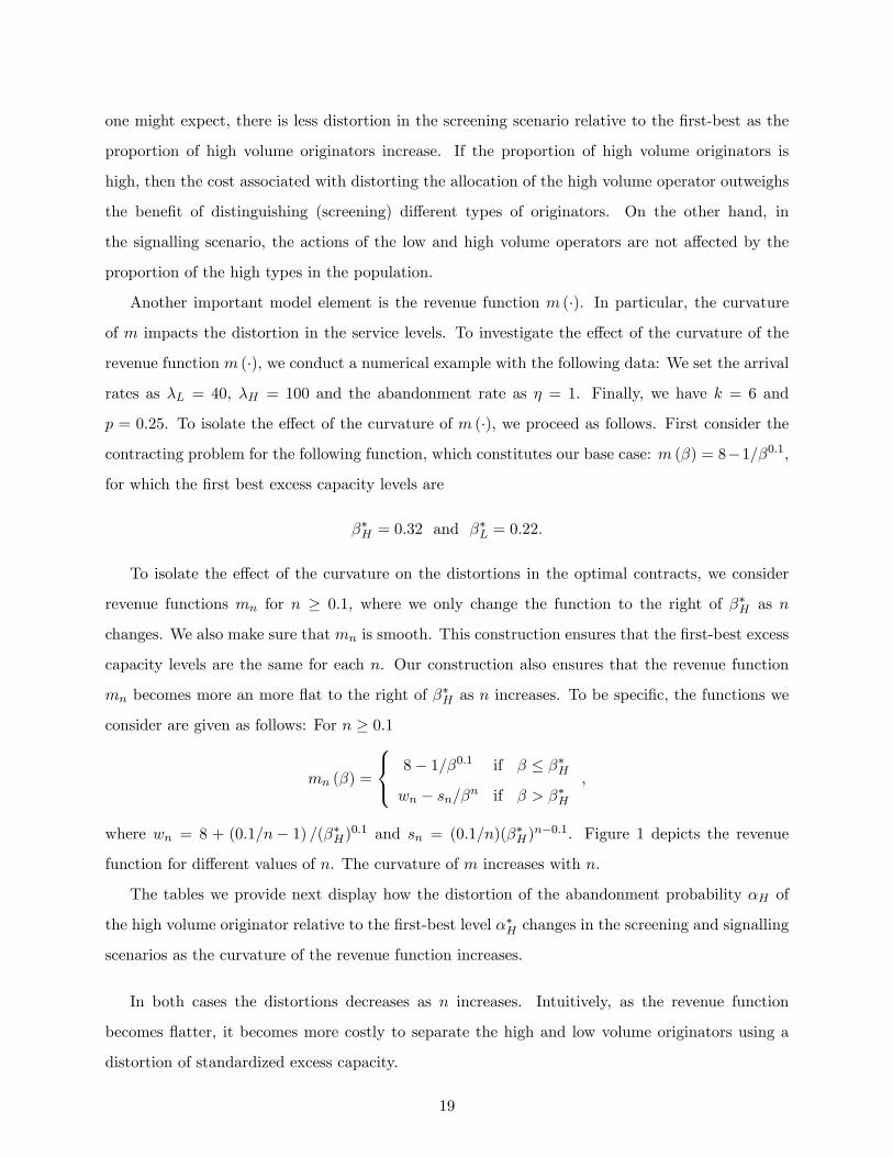
Another important model element is the revenue function m (�). In particular, the curvature

of m impacts the distortion in the service levels. To investigate the e¤ect of the curvature of the

revenue function m (�), we conduct a numerical example with the following data: We set the arrival

rates as �L = 40, �H = 100 and the abandonment rate as � = 1. Finally, we have k = 6 and

p = 0:25. To isolate the e¤ect of the curvature of m (�), we proceed as follows. First consider the

contracting problem for the following function, which constitutes our base case: m (�) = 8�1=�0:1,

for which the �rst best excess capacity levels are

��H = 0:32 and ��L = 0:22.

To isolate the e¤ect of the curvature on the distortions in the optimal contracts, we consider

revenue functions mn for n � 0:1, where we only change the function to the right of ��H as n

changes. We also make sure that mn is smooth. This construction ensures that the �rst-best excess

capacity levels are the same for each n. Our construction also ensures that the revenue function

mn becomes more an more �at to the right of ��H as n increases. To be speci�c, the functions we

consider are given as follows: For n � 0:1

mn (�) =

8<: 8� 1=�0:1 if � � ��Hwn � sn=�n if � > ��H

;

where wn = 8 + (0:1=n� 1) =(��H)0:1 and sn = (0:1=n)(��H)n�0:1. Figure 1 depicts the revenue

function for di¤erent values of n. The curvature of m increases with n.

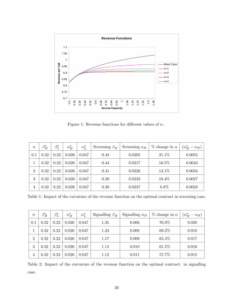
The tables we provide next display how the distortion of the abandonment probability �H of

the high volume originator relative to the �rst-best level ��H changes in the screening and signalling

scenarios as the curvature of the revenue function increases.

In both cases the distortions decreases as n increases. Intuitively, as the revenue function

becomes �atter, it becomes more costly to separate the high and low volume originators using a

distortion of standardized excess capacity.

19

Revenue Functions

6.7

6.75

6.8

6.85

6.9

6.95

7

7.05

7.1

0.2

0.28

0.36

0.44

0.52 0.6

0.68

0.76

0.84

0.92 1

1.08

1.16

1.24

1.32 1.4

1.48

Excess Capacity

Rev

enue

 per

 Cal

l Base Casen=1n=2n=3n=4

Figure 1: Revenue functions for di¤erent values of n.

n ��H ��L ��H ��L Screening �H Screening �H % change in � (��H � �H)

0.1 0:32 0:22 0:026 0:047 0:48 0:0205 21:1% 0:0055

1 0:32 0:22 0:026 0:047 0:44 0:0217 16:5% 0:0043

2 0:32 0:22 0:026 0:047 0:41 0:0226 13:1% 0:0034

3 0:32 0:22 0:026 0:047 0:39 0:0233 10:4% 0:0027

4 0:32 0:22 0:026 0:047 0:38 0:0237 8:8% 0:0023

Table 1: Impact of the curvature of the revenue function on the optimal contract in screening case.

n ��H ��L ��H ��L Signalling �H Signalling �H % change in � (��H � �H)

0.1 0:32 0:22 0:026 0:047 1:35 0:006 76:9% 0:020

1 0:32 0:22 0:026 0:047 1:23 0:008 69:2% 0:018

2 0:32 0:22 0:026 0:047 1:17 0:009 65:4% 0:017

3 0:32 0:22 0:026 0:047 1:14 0:010 61:5% 0:016

4 0:32 0:22 0:026 0:047 1:12 0:011 57:7% 0:015

Table 2: Impact of the curvature of the revenue function on the optimal contract: in signalling

case.

20

References

Aksin, O., de Vericourt, F. & Karaesmen, F. (2006), �Call center outsourcing contract design and choice�,

Management Science . To appear.

Bagwell, K. & Bernheim, B. (1996), �Venlen e¤ects in a theory of conspicuous consumption�, American

Economic Review 86.

Bagwell, K. & Riordan, M. (1991), �High and declining prices signal product quality�, American Economic

Review 81.

Beasty, C. (2005), �The call center outsourcing outlook.�, Business Insights .

Beasty, C. (2006), �Contact center outsourcing strengthens�, Destination CRM.com p. January 17.

Cachon, G. (2003), Supply chain coordination with contracts, Handbooks in Operations Research and Man-

agement Science: Supply Chain Management.

Cachon, G. & Harker, P. (2002), �Competition and outsourcing with scale ecomonies�, Management Science

48(10), 1314�1333.

Cachon, G. & Lariviere, M. P. (2001), �Contracting to assure supply: How to share demand forecasts in a

supply chain�, Management Science 47(5), 629�646.

Cho, I. & Kreps, D. (1987), �Signalling games and stable equilibria�, Quarterly Journal of Economics

102, 179�221.

Choi, J. (1998), �Brand extension as informatioal leverage�, Review of Economic Studies 65.

Chu, W. (1992), �Demand signaling and screening in channels of distribution�, Marketing Science 11(4), 327�

347.

Cohen, L. & Young, A. (2006), Moving beyond outsourcing to Achieve Growth and Agility, Harvard Business

School Press.

Desai, P. & Sirinivasan, K. (1995), �A franchise management issue:Demand signaling under unobservable

service�, Management Science 41(10), 1608�1623.

Garnett, O., Mandelbaum, A. & Reiman, M. (2002), �Designing a call center with impatient customers�,

Manufacturing & Service Operations Management 4, 208�227.

Hasija, S., Pinker, A. & Shumsky, R. (2006), �Call center outsourcing contracts under asymmetric informa-

tion�. Working Paper.

Hassin, R. & Haviv, M. (2002), To Queue or Not to Queue: Equilibrium Behavior in Queueing Systems,

Kluwer Academic Publishers.

21

Milner, J. & Olsen, T. (2007), �Service level agreements in call centers: Perils and prescriptions�,Management

Science . To appear.

Munoz, C. (2007), �External a¤airs.�, The Economist 384, 65�66.

Niezen, C. & Weller, W. (2006), �Procurement as strategy�, Harvard Business Review 84(9), 22�24.

Ren, Z. & Zhang, F. (2007), �Service outsourcing: Information asymmetry and service quality�. Working

paper.

Ren, Z. & Zhou, Y.-P. (2006), �Call center outsourcing: Coordinating sta¢ ng levels and service quality�,

Management Science . Forthcoming.

Salanié, B. (1997), The Economics of Contracts, The MIT Press.

Schultz, C. (1996), �Polarization and ine¢ cient policies�, Review of Economic Studies 63.

Taylor, R. & Tofts, C. (2006), �Death by a thousand slas; A short study of commerical suicide pacts.�.

working paper. HP Laboratories Bristol.

A Proofs in Sections 2.1 and 3

Proof of Proposition 1. The �rst order condition, which is necessary and su¢ cient by Assump-

tion 1, gives �m(��)(1� �(�

�)p�)

�0= k=

p�.

By Assumption 1, we have �� is increasing in �. Then, �� is decreasing since � is decreasing. �

Lemma 1 The constraints (IRH) and (ICL) of the service provider�s screening problem bind at an

optimum contract.

Proof of Lemma 1. Suppose (IRH) does not bind. Then, increasing cH by a small amount

is more pro�table to the service provider. Clearly, we can do this if (ICH) does not bind, because

increasing cH relaxes (ICL). Therefore, we restrict attention to the possibility that (ICH) binds.

In that case, we have that

(1� �H)[m(�(�H ; �H))� cH ] = (1� �L)[m(�(�L; �H))� cL]: (22)

Since (IRH) does not bind by assumption, we have m(�(�H ; �H)) > cH . Then, (22) implies that

m(�(�L; �H)) > cL as well. Because cL and cH are related through (22), we need to check that

22

(IRL) is not violated as we increase cH by a small amount. Thus, we next consider (IRL). Since

m (�) is increasing and �(�L; �L)) > �(�L; �H), we have

m(�(�L; �L))� cL � m(�(�L; �H))� cL > 0:

Therefore, (IRL) does not bind either. Then, consider increasing cH by �1��H and cL by �

1��L

for su¢ ciently small � > 0. Then, the incentive compatibility constraints are not violated since

we decrease both sides by �; but the objective value of the service provider�s screening problem

increases strictly, which contradicts optimality. Thus, (IRH) binds at an optimum contract.

Now suppose that (ICL) does not bind. Since (IRH) binds by the above argument, we have

that m(�(�H ; �H)) = cH . Then, ICL becomes

(1� �L)[m(�(�L; �L))� cL] > (1� �H)[m(�(�H ; �L))�m(�(�H ; �H))];

where the right hand side is strictly positive since �(�H ; �L) > �(�H ; �H), which implies that (IRL)

does not bind either. Also note that increasing cL by a su¢ ciently small � > 0 relaxes (ICH). Thus,

we can increase cL by a su¢ ciently small � > 0, in which case (IRL) and (ICL) are still satis�ed

and we get a strictly better objective value, contradicting the optimality. Thus, (ICL) binds. �

Proof of Proposition 2. First notice that we have the following relations for any given

abandonment probabilities �L and �H :

�(�L; �H) � �(�L; �L);

�(�H ; �L) � �(�H ; �H);

which is due to statistical economies of scale inherent in queueing systems. Also recall that (IRH)

and (ICL) binds at an optimum contract by Lemma 1. Then, (IRL) is also satis�ed since

�L(1� �L)[m(�(�L; �L))� cL] = �L(1� �H)[m(�(�H ; �L))� cH ];

� �L(1� �H)[m(�(�H ; �H))� cH ];

= 0;

where the �rst equality follows from the fact that (ICL) binds, the second line is true since

�(�H ; �L) � �(�H ; �H) and the last line follows from (IRH).

We proceed with the service provider�s screening problem ignoring the constraint (ICH) for now.

We will �rst characterize the optimal solution to a relaxed problem, which ignores (ICH), and then

23

verify that (ICH) is indeed satis�ed by that solution in the end. Given that (IRH) and ICL bind

by Lemma 1, we can solve for cH and cL, which gives the following:

cH = m(�(�H ; �H)); (23)

cL = m(�(�L; �L)) +(1� �H)(1� �L)

[m(�(�H ; �H))�m(�(�H ; �L))]: (24)

Then, substituting (23) and (24) into the objective function of the service provider�s problem

(ignoring (ICH) for now) we arrive at the following problems. Choose the abandonment probabilities

�L and �H so as to maximize

p[m(�(�H ; �H))�H(1� �H)� k(�H +p�H�(�H ; �H))]� (1� p)k(�L +

p�L�(�L; �L))

+(1� p)��m(�(�L; �L)) +

(1� �H)(1� �L)

[m(�(�H ; �H))�m(�(�H ; �L))]��L(1� �L)

�(25)

It is easy to see that the optimal level of �L is equal to ��L, the �rst-best level. To �nd the

optimum �H , we consider the following problem, which ignores the terms that do not depend on

�H : Choose the abandonment probability �H for the high type so as to

maximize�H p[m(�(�H ; �H))�H(1� �H)� k(�H +p�H�(�H ; �H))]

+(1� p) [((1� �H)[m(�(�H ; �H))�m(�(�H ; �L))])�L] : (26)

By (3), the maximization problem (26) can equivalently be stated as a problem of choosing the

optimal standardized excess capacity �H as follows: Choose �H so as to

maximize p[m(�H)�H

�1� �(�H)p

�H

�� k(�H +

p�H�H)]

+(1� p)�L��1� �(�H)p

�H

�[m(�H)�m(b�H)]� ; (27)

where b�H is de�ned as a function of �H through the relation�(�H)p�H

=�(b�H)p�L

:

The �rst order conditions for (27) give�m(�H)

�1� �(�H)p

�H

��0=

kp�H

� (1� p)�Lp�H

��1� �(�H)p

�H

�[m(�H)�m(b�H)]�0 ; (28)

where the second termh(1� �(�H)p

�H)[m(�H)�m(b�H)]i0 � 0 by Assumption 2. To see this, notice

that Assumption 2 can be rewritten as follows using simple algebraic manipulations:

(1� �)[m(��1(�p�))�m(��1(�

p��))] is decreasing as (1� �) increases for � > 1:

24

Then, the termh(1� �(�H)p

�H)[m(�H)�m(b�H)]i can be expressed as a function of the abandonment

probability �H through the relation (3) as follows:

(1� �H)hm���1

��Hp�H

���m

���1

��Hp�L

��i;

which is nonpositive and increasing as �H decreases by Assumption 2. This is equivalent to haveh(1� �(�H)p

�H)[m(�H)�m(b�H)]i increasing as a function of �H , cf. (3). Then comparing (5) with

(28) yields �H � ��H by Assumption 1, which in turn implies, cf. (2), that

�H =�(�H)p�H

� �(��H)p�H

= ��H < ��L = �L:

Then it follows from Assumption 2 that

(1� �L)hm���1

��Lp�L

���m

���1

��Lp�H

��i� (1� �H)

hm���1

��Hp�L

���m

���1

��Hp�H

��i;

which in turn is equivalent to (cf. 3)

(1� �L)[m(�(�L; �L))�m(�(�L; �H))] � (1� �H)[m(�(�H ; �L))�m(�(�H ; �H))]: (29)

Recall that we had ignored (ICH) while we solve the above maximization problem. What

remains is to check whether (ICH) is satis�ed in this solution. For that,the right hand side of

(ICH) is zero, since (IRH) binds. Then rewrite (ICH) as follows:

0 � (1� �L)[m(�(�L; �H))� cL]: (30)

Substituting (24) into (30), an rearranging terms we see that checking whether (ICH) is satis�ed

is equivalent to checking whether the following holds:

(1� �L)[m(�(�L; �L))�m(�(�L; �H))] � (1� �H)[m(�(�H ; �L))�m(�(�H ; �H))];

which is precisely (29). Thus, (ICH) is satis�ed.

Finally, note that the high type originator earns zero pro�ts by (23); and it follows from (24)

and the fact that m(�(�H ; �L)) > m(�(�H ; �H)) that the low type originator gets strictly positive

information rent. �

25

B Proofs and Auxiliary Derivations for Section 4

In this appendix, we prove the results in Section 4 and provide some auxiliary results necessary

for proofs. We also reviews the formal de�nition of the intuitive criterion of Cho & Kreps (1987),

which we specialize for our setting.

Intuitive Criterion. The idea of this re�nements is that reasonable beliefs should not assign

positive probability to a player taking an action that is strictly dominated (in a sense to be made

precise) for her. To formalize this, for any nonempty set � � fH;Lg, let S�(�; (c; �)) � fAccept,

Rejectg denote the set of possible equilibrium responses by the service provider that can arise after

contract o¤er (c; �) is observed for some beliefs satisfying the property that �(c; �) = 1 if � = fHg

and �(c; �) = 0 if � = fLg. That is, the set S�(�; (c; �)) contains the equilibrium responses by

the service provider to the contract choice (c; �) for some beliefs that assign positive probability to

types only in the set �. When we have � = fH;Lg, this construction puts no restriction on the

beliefs.

We now introduce the notion of equilibrium dominance. To facilitate our analysis, we introduce

the following de�nitions with a slight abuse of notation. Let �H(c; �; s) denote the pro�t of a high

type originator if she o¤ers the contract (c; �) and the service provider�s decision is s 2 fAccept,

Rejectg. Then, we have

�H(c; �;Accept) = (1� �)�H [m(��1(�p�H))� c] and �H(c; �;Reject) = 0.

Similarly de�ne �L(c; �; s) as the pro�t of the low type originator if she o¤ers a contract (c; �)

and the service provider�s decision is s 2 fAccept, Rejectg: Let (cH ; �H) and (cL; �L) denote the

contract o¤ers of the high and low type originators in a perfect Bayesian equilibrium with belief

system �. The equilibrium responses by the call center to the contract o¤ers (cH ; �H) and (cL; �L)

should be to accept since otherwise the originator would not be maximizing her payo¤. We then say

that a contract (c; �) is equilibrium dominated for the high type in this perfect Bayesian equilibrium

if

(1� �H)�H [m(��1(�Hp�H))� cH ] > Maxs2S�(fH;Lg;(c;�)) �H(c; �; s). (31)

We similarly de�ne the contracts that are equilibrium dominated for the low type. Then, for each

contact (c; �), we de�ne the set ��(c; �) as the set of types for which (c; �) is not equilibrium

dominated. Finally, the perfect Bayesian equilibrium with contract o¤ers (cH ; �H) and (cL; �L)

and belief system � is said to violate the intuitive criterion if there exists a type � 2 fH;Lg and a

26

contract (c; �) such that

Mins2S�(��(c;�); (c;�)) ��(c; �; s) > ��(c�; ��;Accept). (32)

For instance, a pooling equilibrium with contract o¤er (ec; e�) and the belief system � violate the

intuitive criterion if there exists a type � and a deviation (c; �) that yields higher pro�t for type

� than her equilibrium pro�t as long as the call center does not assign a positive probability to a

type for which the deviation (c; �) is equilibrium dominated.

The following lemma is nothing but the "if part" of Proposition 3, which is really what is needed

for the following proofs. Thus, we next state and prove Lemma 2; and we will eventually prove

the "only if" part of Proposition 3, which provides a criterion (in terms of problem primitives)

equivalent to the intuitive criterion in our setting.

Lemma 2 A perfect Bayesian equilibrium with contract o¤ers (cL; �L) an (cH ; �H) violate the

intuitive criterion of Cho & Kreps (1987) if there exists a type i 2 fL;Hg and a deviation contract

(ec; e�) such that�i(e�i;eci) > �i(�i; ci), �j(�j ; cj) > �j(e�i;eci) and (1�e�i)eci�i�k(�i+p�i��1(e�ip�i)) � 0 for j 6= i.

(33)

Proof of Lemma 2. In any equilibrium we have �i(ci; �i;Accept) � 0 for i = L;H. Thus, in

(32), we should have S�(��(c; �); (c; �)) = fAcceptg. This, in turn, implies that a contract (�; c)

is a deviation for type i = L;H violating the intuitive criterion if �i(�; c) > �i(�i; ci), �j(�j ; cj) >

�j(�; c) for j 6= i (which guarantees that ��(c; �) = fig) and (1��)c�i�k(�i+p�i�

�1(�p�i)) � 0

(which ensures S�(��(c; �); (c; �)) = fAcceptg). �

We will use the following lemma to construct deviations of the form given in Lemma 2; and

we will eventually prove the "only if" part of Proposition 3, which provides a criterion at various

places in what follows.

Lemma 3 Consider candidate equilibrium contract o¤ers (cL; �L) and (cH ; �H) (not necessarily

di¤erent, i.e. we allow for (cL; �L) = (cH ; �H)) o¤ered by the low and high type originators,

respectively. If �H (cH ; �H) = �H (cL; �L), then there exists a deviation (�; c) for the high type

such that

�H(�; c) > �H(�H ; cH), �L(�L; cL) > �L(�; c) and (1� �)c�H � k(�H +p�H�

�1(�p�H)) � 0.

27

Thus, f(cL; �L) ; (cH ; �H)g cannot correspond to outcomes of a perfect Bayesian equilibrium satis-

fying the intuitive criterion.

Proof of Lemma 3. To construct such a deviation for the high type, choose � < �L and set

c such that

(1� �)c = (1� �L)cL +1

2

h(1� �)m(��1(�

p�L))� (1� �L)[m(��1(�L

p�L))

i+1

2

h(1� �)m(��1(�

p�H))� (1� �L)[m(��1(�L

p�H))

i: (34)

Recall that1

�L�L(�; c) = (1� �)m(��1(�

p�L))� (1� �)c:

Then substituting (34) into this and rearranging terms give

1

�L�L(�; c) = (1� �L)m(��1(�L

p�L))� (1� �L)cL

�12(1� �L)

hm(��1(�L

p�L))�m(��1(�L

p�H))

i+1

2(1� �)

hm(��1(�

p�L))�m(��1(�

p�H))

i< (1� �L)m(��1(�L

p�L))� (1� �L)cL; (35)

where the last inequality follows from Assumption 2. Then, (35) can equivalently be written as

�L(�; c) < (1� �L)�Lhm(��1(�L

p�L))� cL

i= �L(�L; cL):

Similarly we have that

1

�H�H(�; c) = (1� �)m(��1(�

p�H))� (1� �)c:

Then substituting (34) into this and rearranging terms give

1

�H�H(�; c) = (1� �L)m(��1(�L

p�H))� (1� �L)cL

+1

2(1� �L)

hm(��1(�L

p�L))�m(��1(�L

p�H))

i�12(1� �)

hm(��1(�

p�L))�m(��1(�

p�H))

i> (1� �L)m(��1(�L

p�H))� (1� �L)cL; (36)

where the inequality follows from Assumption 2. Clearly, (36) is equivalent to

�H(�; c) > (1� �L)�Hhm(��1(�L

p�H))� cL

i;

28

where the right hand side is equal to �H(�L; cL) by de�nition, which, in turn, is equal to �H(�H ; cH)

by assumption. Thus, we have

�H(�; c) > �H(�H ; cH):

Moreover, since (�L; cL) and (�H ; cH) are equilibrium outcomes, the service provider will assign

positive probability to the originator being a low type upon seeing the contract o¤er (�L; cL), that

is, 1� �(�L; cL) > 0. Given the service provider accepts the contract o¤er (�L; cL) in equilibrium,

we must have

�(cL; �L)

�(1� �L)cL � k(1 +

��1(�Lp�H)p

�H)

�+(1��(cL; �L))

�(1� �L)cL � k(1 +

��1(�Lp�L))p

�L

�� 0:

Then we have that

(1� �L)cL � k�1 +

��1(�Lp�H)p

�H

�> 0;

which follows since

0 � �(cL; �L)

�(1� �L)cL � k(1 +

��1(�Lp�H)p

�H)

�+(1� �(cL; �L))

�(1� �L)cL � k(1 +

��1(�Lp�L))p

�L

�< (1� �L)cL � k

�1 +

��1(�Lp�H)p

�H

�:

Then we also have that

(1� �)c� k�1 +

��1(�p�H)p

�H

�� 0

for � < �L su¢ ciently close to �L. Thus,

(1� �)c�H � k��H +

p�H�

�1(�p�H)

�� 0:

The proof is then complete by Lemma 2. Finally, note that nowhere in this proof we assumed

(cL; �L) 6= (cH ; �H).Thus, this result can be used to construct deviations from a pooling equilibrium

as well. �

Next, we prove Proposition 4.

Proof of Proposition 4. We follow the 4-step approach outlined next.

Step 1: Characterize a perfect Bayesian equilibrium as a solution to an optimization problem.

Step 2: Characterize/solve the optimization problem identi�ed in Step 1.

Step 3: Show that the equilibrium characterized in Step 2 satis�es the intuitive criterion.

Step 4: Check that the only perfect Bayesian separating equilibrium satisfying the intuitive

criterion is the one characterized in Step 2.

29

Step 1. Here we �rst focus on a speci�c separating equilibrium where the out of equilibrium

beliefs are de�ned as follows: The service provider believes the originator to be a low type if

he sees a contact o¤er di¤erent than (cH ; �H), the equilibrium contract o¤er of the high type

originator. We will eventually show that the equilibrium we derived under this belief system is the

unique (pure strategy) perfect Bayesian equilibrium satisfying the intuitive criterion without any

speci�c assumptions on the belief system. To this end, we �rst derive the constraints which have

to be satis�ed by a pair f(cL; �L); (cH ; �H)g of separating equilibrium contract o¤ers. Consider

the contract choice of the low type under the belief system � that assigns probability zero to the

originator being a high type upon seeing a contract o¤er other than (cH ; �H). Then, the contract

o¤er (cL; �L) is sequentially rational for the low type if it yields a pro�t that is better than any

possible deviation. If the low type deviates to a contract (c; �) 6= (cH ; �H), then the service provider

believes she is a low type. Thus, if (c; �) is accepted by the service provider, the low type gets

pro�t �L(c; �). Therefore, the best deviation for the low type to a contract (c; �) 6= (cH ; �H), then

solves the following maximization problem: Choose the contract o¤er (c; �) so as to

maximize �L(c; �)

subject to

(1� �)c�L � k(�L +p�L�

�1(�p�L)) � 0:

The constraint in this maximization problem always binds. Thus, the problem is the same as

maximizing the surplus in the system. The solution is given by the �rst best level � = ��L as in

(5)-(6), and we have

(1� ��L)c�L = k(1 +��1(��L

p�L)p

�L):

Therefore, any deviation for the low type to a contract (c; �) 6= (cH ; �H) yields less pro�t for the

low type. Then, for (cL; �L) = (c�L; ��L) to be sequentially rational, it should also give higher pro�ts

for the low type than the equilibrium contract o¤er (cH ; �H) of the high type. That is, we must

have

�L(c�L; �

�L) � (1� �H)�L[m(��1(�H

p�L))� cH ]: (37)

We next consider the sequential rationality of the contract choice (cH ; �H) of the high type. If

the high type deviates from (cH ; �H), under the belief system �, the call center will believe that she

is a low type. Thus, the best such deviation will solve the following problem: Choose the contract

30

o¤er (c; �) so as to

maximize �H(c; �) (38)

subject to

(1� �)c�L � k(�L +p�L�

�1(�p�L)) � 0: (39)

Note that the constraint (39) re�ects the fact that the service provider accepts the contract believing

that it is o¤ered by a low type originator. It is easy to see that the constraint (39) will always bind

in optimum contract solving the problem (38)-(39). Thus, we can equivalently state (38)-(39) as

follows: Choose the abandonment probability � so as to

maximize (1� �)m(��1(�p�H))� k(1 +

��1(�p�L)p

�L): (40)

which, in turn, can also be posed as a problem of choosing the standardized capacity � to

maximize (1� �(�)p�H)m(�)� k(1 +

b�p�L); (41)

where b� is de�ned as a function of � implicitly through the relation�(�)p�H

=�(b�)p�L: (42)

The �rst order condition associated with the problem (41) can be written as�m(�)(1� �(�)p

�H)

�0=

kp�L

@b�@�; (43)

where @b�=@� can be calculated using the implicit function theorem. More speci�cally, de�ne thefunction ' such that

'(b�; �) = �(b�)�r �L�H�(�) = 0:

We have that

@b�=@� = �@'=@�@'=@b� =

r�L�H

�0(�)

�0(b�) :Substituting this into (43), the �rst order condition becomes�

m(�)(1� �(�)p�H)

�0=

kp�H

�0(�)

�0(b�) ; (44)

where the right hand side is strictly less than k=p�H since b� > � and �

0(b�) > �

0(�). Then

comparing (44) with (5) and using Assumption 1, we see that the optimum solution e� to the31

problem (42) satis�es e� > ��H , where ��H is the �rst best level. This implies that the optimal

abandonment probability e� for the problem 38)-(39), or equivalently for the problem (40), satis�es

e� = ��e��p�H

< ��H ; (45)

where ��H is the �rst-best abandonment probability. Thus, the sequential rationality of (cH ; �H)

requires that

�H(cH ; �H) � �H eg(e�); (46)

where

eg(�) = (1� �)m(��1(�p�H))� k(1 + ��1(�p�L)p�L

):

The last constraint the contract (cH ; �H) has to satisfy is that it has to be accepted by the call

center. Since �(cH ; �H) = 1; this translate into the constraint

(1� �H)cH�H � k(�H +p�H�

�1(�Hp�H)) � 0: (47)

In summary, for (cL; �L) and (cH ; �H) to be equilibrium contract o¤ers we must have (cL; �L) =

(c�L; ��L) and that (cH ; �H) should solve the following problem: Choose (c; �) so as to

maximize �H(c; �) (48)

subject to

(1� �)c�H � k(�H +p�H�

�1(�p�H)) � 0; (49)

�H(c; �) � �Heg(e�); (50)

�L(c�L; �

�L) � (1� �)�L[m(��1(�

p�L))� c]: (51)

The problem (48)-(51) characterizes the equilibrium contract o¤ers, completing Step 1.

Step 2. We now focus on solving the problem (48)-(51). Clearly, we can reformulate the problem

(48)-(51) as one of choosing (1� �H)cH and �H . Without loss of generality, set

"H = k(1 +��1(�H

p�L)p

�L� (1� �H)cH : (52)

Then,we can rewrite the problem as one of choosing "H and �H optimally. Substituting (52) into

(49)-(51), we can write the constraints as follows:

"H � h(�H);

"H � eg(e�)� eg(�H);"H � gL(�L)� gL(�H),

32

where h(�) and gL(�) are de�ned as

h(�) = k

���1(�

p�L)p

�L� �

�1(�p�H)p

�H

�, gL(�) = (1��)[m(��1(�

p�L))]�k

�1 +

��1(�p�L)p

�L

�:

Then, we can equivalently express the problem (48)-(51) as choosing "H and �H so as to

maximize eg(�H) + "Hsubject to

"H � h(�H);

eg(e�)� eg(�H) � "H � gL(�L)� gL(�H).We further simplify the problem as follows: Choose "H and �H to

maximize eg(�H) + "H (53)

subject to

"H + eg(�H) � gH(�H); (54)

eg(e�) � "H + eg(�H) � gL(�L)� gL(�H) + eg(�H), (55)

where gH(�) = h(�) + eg(�) = (1��)[m(��1(�p�H))]� k �1 + ��1(�p�H)p

�H

�. That is, we consider

the following maximization problem in which we choose �; �H so as to

maximize � (56)

subject to

� � gH(�H); (57)

eg(e�) � � � f(�H), (58)

where f(�) = gL(�L) � gL(�) + eg(�). To characterize the solution to the problem (56)-(58), we

make the following observations.

Observation 1:

(i) gH(�) achieves its unique maximum at ��H .

(ii) gH(�) > eg(�) for all � 2 (0; 1]. Moreover, gH(�) > gH(e�) > eg(e�) for e� < � < ��H .(iii) There exists a unique �< e� such that gH(�) = eg(e�):It is easy to see that part (i) follows from Assumption 1 and the �rst order condition (??). We

have gH(�) > eg(�) for all � 2 (0; 1] since � is decreasing and �H > �L. Then, gH(�) > gH(e�) >33

eg(e�) for e� < � < ��H from Part (i). Part (iii) simply follows from Part (ii) and monotonicity of

gH .

Observation 2: f(�) is decreasing with f(��H) < gH (��H) and f (�) > gH(�) = eg(e�).Assumption 2 implies that f(�) is decreasing. We have f(��H) = gL(�L) � gL(��H) + eg(��H) <

gH(��H) since gL(�L) < gH(�

�H) and gL(�

�H) > eg(��H). Finally, f (�) > gH(�) = eg(e�) since

f (e�) > eg(e�), f(�) if decreasing and �< e�.Observation 3: There exists a unique �H 2 (�; ��H) such that f (�H) = gH (�H), which also

satis�es f (�H) > eg(e�). Moreover, (cH ; �H), wherecH =

k

(1� �H)

�1 +

��1(�Hp�H)p

�H

�; (59)

is the unique optimal solution of (48)-(51).

To see why �H and cH as in (59) is the unique optimal solution of (48)-(51), recall that the

constraint (57), or equivalently (54), binds at an optimum solution. Then, since the constraint

(57) was obtained from (50) through the relation (52), "H denote the slack in (50). The fact that

(57) binds at the optimum implies that "H = 0 and hence, �H and cH as in (59) constitute an

equilibrium contract o¤er for the high type.

Therefore, (c�L; ��L) and (cH ; �H) as characterized in Observation 3 are the equilibrium contract

o¤ers by the low and high types, under the belief system �. The next step is to this equilibrium

satis�es the intuitive criterion.

Step 3.

Let (c�L; ��L) and (cH ; �H) denote the contract o¤ers by the high and low type originators in the

separating equilibrium of Step 2. The high and low type originators earn the following pro�ts:

�H(cH ; �H) = (1� �H)[m(��1(�Hp�H))� cH ];

�L(c�L; �

�L) = (1� ��L)m(��1(��L

p�L))� k(�L +

p�L�

�1(��Lp�L)):

We will show that there for both the low and high types, there exists no deviation that would

violate the intuitive criterion. We �rst consider the potential deviations by the low type. Since we

have

�L(c�L; �

�L)) > 0;

the low type would not deviate to a contract that would be rejected by the call center. Put more

formally, for there to be a deviation (c; �) for the low type such that

Mins2S�(��(c;�); (c;�)) uL(c; �; s) > �L(c�L; �

�L)),

34

we should have that S�(��(c; �); (c; �)) = fAcceptg. Suppose such a deviation (c; �) exists.

This immediately implies that uL(c; �;Accept) > uL(c�L; �

�L;Accept). Thus, fLg � ��(c; �) if

��(c; �) 6= ?. Recall that by de�nition, the set S�(��(c; �); (c; �)) contains the equilibrium

responses by the call center to the contract choice (c; �) for some beliefs that assign positive

probability to types only in the set ��(c; �). Then, to have S�(��(c; �); (c; �)) = fAcceptg, the

contract (c; �) has to satisfy

�L(1� �)c� k(�L +p�L�

�1(�p�L)) � 0;

in which case we have

uL(c; �;Accept) � uL(cL; �L;Accept);

as ��L is the �rst best level of abandonment rate for the low type, contradicting the assumption

that (c; �) is a deviation that yields higher for the low type originator.

Second we consider potential deviations by the high type originator. Suppose there exists a

contract o¤er (c; �) 6= (cH ; �H) by the high type such that

Mins2S�(��(c;�); (c;�)) uH(c; �; s) > uH(cH ; �H).

Since (cH ; �H) gives the high type originator nonnegative pro�ts, we should have S�(��(c; �);

(c; �)) = fAcceptg. Then, since uH(c; �;Accept) > uH(cH ; �H ;Accept), we have fHg � ��(c; �).

Now consider two cases that might potentially arise. In the �rst case, we have ��(c; �) = fHg. If

��(c; �) = fHg, to have S�(��(c; �); (c; �)) = fAcceptg, it should be that

�H(1� �)c� k(�H +p�H�

�1(�p�H)) � 0:

Moreover, by the de�nition of the set ��(c; �) = fHg; we must also have

(1� ��L)[m(��1(��Lp�L))� c�L] > (1� �)[m(��1(�

p�L))� c];

(1� �H)[m(��1(�p�H))� cH ] < (1� �)[m(��1(�

p�H))� c];

However, this would contradict the sequential rationality of the contract choice (cH ; �H) in the

separating equilibrium Step 2. Thus, there exits no deviation (c; �) for the high type such that

��(c; �) = fHg and the intuitive criterion is violated.

In the second case, we have ��(c; �) = fH;Lg. If ��(c; �) = fH;Lg, then to have S�(��(c; �);

(c; �)) = fAcceptg, we must have

�L(1� �)c� k(�L +p�L�

�1(�p�L)) � 0: (60)

35

Then, the best possible pro�t a the high type originator could get from a deviation (c; �) that

satisfy (60) is

(1� e�)�H �m(��1(e�p�H))� k(1 + ��1(e�p�L)p�L

�,

where e� is given by (45). From (46), the deviation (c; �) yields less pro�ts for the high type

originator than uH(cH ; �H). Thus, no deviation exists for the high type that would violate the

intuitive criterion and the equilibrium in Step 2 satis�es the intuitive criterion.

Step 4. We now show that the separating equilibrium characterized in Step 2 is the unique

outcome that might arise as a separating equilibrium satisfying the intuitive criterion.

To check this, let f(cH ; �H) ; (cL; �L)g be an arbitrary separating equilibrium contract o¤ers

satisfying the intuitive criterion. First, we show that we must have

(1� �L)cL = k�1 +

��1(�Lp�L)p

�L

�: (61)

That is, the contract o¤er of the low type originator does not leave any surplus to the service

provider. Second, we show that we must have �L = ��L. Finally, we show that �H and cH are as

characterized in Step 2. In particular, they satisfy

�H < ��H and (1� �H)cH = k

�1 +

��1(�Hp�H)p

�H

�:

To show that (61) holds, we argue by contradiction. Note that in a separating equilibrium,

upon seeing the low type�s contract o¤er (cL; �L), the service provider knows that she is low type.

Since the service provider accepts the contract o¤ered in equilibrium, we must have that

(1� �L)cL � k�1 +

��1(�Lp�L)p

�L

�:

Thus, we only need to rule out the possibility that

(1� �L)cL > k�1 +

��1(�Lp�L)p

�L

�: (62)

Suppose (62) holds. Then, (cL � �; �L) for � > 0 su¢ ciently small is a deviation that violate the

intuitive criterion. To see this, it su¢ ces to check that �H(�H ; cH) > �H(�L; cL � �), cf. Lemma

2. By incentive compatibility, we must have �H(�H ; cH) � �H(�L; cL). Then, if �H(�H ; cH) >

�H(�L; cL), we also have �H(�H ; cH) > �H(�L; cL � �) for � small enough. Therefore, we restrict

attention to the case �H(�H ; cH) = �H(�L; cL), that is, the high type is indi¤erent between his

contract and that of the low type, but then one can invoke Lemma 3 to �nd a deviation (c; �) for

the high type originator such that

�H(�; c) > �H(�H ; cH), �L(�L; cL) > �L(�; c) and (1� �)c�H � k(�H +p�H�

�1(�p�H)) � 0,

36

which is a contradiction. Thus, the low type extracts all the surplus from the service provider in

any separating equilibrium satisfying the intuitive criterion.

Next, we prove that �L = ��L, for which we use the fact that

(1� �L)cL = k�1 +

��1(�Lp�L)p

�L

�: (63)

We argue by contradiction, i.e. suppose �L 6= ��L. If �H(�H ; cH) > �H(�L; cL), then moving

slightly towards ��L would be a deviation for the low type that violates the intuitive criterion. On

the other hand, if �H(�H ; cH) = �H(�L; cL), the argument is the same as the one immediately

above. Namely, the high type can �nd a deviation that violates the intuitive criterion. Thus, we

have �L = ��L:

Finally, we prove that �H and cH are as characterized in Step 2. in particular, we shoe that

they satisfy

�H < ��H and (1� �H)cH = k

�1 +

��1(�Hp�H)p

�H

�:

To this end, let (�H ; cH) denote the speci�c contract o¤er of the high type characterized in Step

2. Since we already know that �L = ��L and cL is as in (63), we need to only consider deviations

by the high type. We argue by contradiction. Suppose (�H ; cH) 6= (�H ; cH). Then, it follows from

the proof of Step 2 that if

�H > �H and (1� �H)cH = k(1 +��1(�H

p�H)p

�H);

then the low type will prefer (�H ; cH) over (�L; cL). Then it is easy to show that there exists a

deviation for the low type violating the intuitive criterion as in Lemma 2. on the other hand if

�H > �H and (1� �H)cH > k(1 +��1(�H

p�H)p

�H);

then the contract (�H ; cH � �) for � small enough yields strictly better pro�ts for the high type,

and we will have

(1� �H) (cH � �) > k(1 +��1(�H

p�H)p

�H):

Moreover, we would have �L (�H ; cH � �) < �L (�L; cL) if �L (�H ; cH) < �L (�L; cL) already.

Therefore we restrict attention to the case �L (�H ; cH) = �L (�L; cL). Then, there exists a de-

viation (�; c) for the high type such that �H(�H ; cH) < �H(�; c), �L(�H ; cH) > �L(�; c) and

(1 � �)c�H � k(�H +p�H�

�1(�p�H)) � 0, which follows from Lemma 3, and that violates the

intuitive criterion by Lemma 2. Thus, we have proved that we cannot have �H > �H .

37

We next show that we cannot have �H < �H . If �H < �H and

(1� �H)cH = k(1 +��1(�H

p�H)p

�H);

then the high type can increase �H slightly and set

(1� �H)cH = k(1 +��1(�H

p�H)p

�H);

which will yield strictly higher pro�ts for her, while the low type would strictly prefer

�L = ��L and (1� ��L)cL = k(1 +

��1(��Lp�L)p

�L)

over the deviation of the high type since �L(�H ; cH) < �L(�L; cL) for �H < �H and (1��H)cH =

k(1 + ��1(�Hp�H)p

�H). Then what remains to show is that �H < �H and (1 � �H)cH > k(1 +

��1(�Hp�H)p

�H) cannot be an equilibrium outcome in a separating equilibrium satisfying the intuitive

criterion. If �L(�H ; cH) < �L(�L; cL), then (�H ; cH � �) for � small enough is a deviation for the

high type that violates the intuitive criterion. Finally, observe that we cannot have �L(�H ; cH) =

�L(�L; cL) if �H < �H and

(1� �H)cH > k(1 +��1(�H

p�H)p

�H)

since �L(�H ; cH) = �L(�L; cL). Thus, we have that �H = �H .

Finally we show that

(1� �H)cH = k(1 +��1(�H

p�H)p

�H):

We argue by contradiction again. Suppose that

(1� �H)cH > k(1 +��1(�H

p�H)p

�H):

Then, �L(�H ; cH) < �L(�L; cL) by the proof of Step 2. Hence, (�H ; cH � �) for � small enough is

a deviation for the high type that violates the intuitive criterion. Thus, we have �H = �H and

(1� �H)cH = k(1 +��1(�H

p�H)p

�H);

which prove that �H and cH are as characterized in Step 2. �

Proof of Proposition 5. We argue by contradiction. Suppose that there exists a pooling

equilibrium that satis�es the intuitive criterion. Let (ec; e�) denote an arbitrary pooling equilibriumcontract o¤er with the belief system �. From Bayes�rule, we have �(ec; e�) = p. Note that (ec; e�)has to be accepted by the service provider since otherwise some type would �nd it pro�table to

38

deviate and o¤er a contract that is accepted. Since (ec; e�) is accepted in the equilibrium by the

service provider, we have

ph(1� e�)ec�H � k(�H +p�H��1(e�p�H))i+(1�p) h(1� e�)ec�L � k(�L +p�L��1(e�p�L))i � 0:

Next, we show that the high type has a deviation that violates the intuitive criterion. It is easy to

see that there exists a deviation (c; �) for the high type as in Lemma 3 deviation contract (ec; e�)such that

�H(c; �) > �H(ec; e�), �L(ec; e�) > �L(c; �) and (1� �)c�H � k(�H +p�H��1(�p�H)) � 0,which is a contradiction. Thus, there exists no pooling equilibrium that satis�es the intuitive

criterion. �

Proof of Proposition 3. The "if part" of Proposition 3 was established in Lemma 2. We

now prove the "only if" part of Proposition 3. Namely, we prove that if for a perfect Bayesian

equilibrium with contract o¤ers (�L; cL) and (�H ; cH), there exists no type i 2 fL;Hg and no

deviation contract (�; c) such that

�i(�; c) > �i(�i; ci), �j(�j ; cj) > �j(�; c) and (1� �)c�i � k(�i +p�i�

�1(�p�i)) � 0 for j 6= i,

then the perfect Bayesian equilibrium with contract o¤ers (�L; cL) and (�H ; cH) does not violate

the intuitive criterion. We have shown in Step 4 of the proof of Proposition 4 that the only perfect

Bayesian separating equilibrium for which there exists no deviations as in Lemma 2 is the one

characterized in Proposition 4. Moreover, we have also shown that the equilibrium characterized

in Proposition 4 satis�es the intuitive criterion, This establishes that if for a perfect Bayesian

equilibrium, there exits no deviations as in Lemma 2, then the perfect Bayesian equilibrium satis�es

the intuitive criterion. �

39

C Proofs in Section 5

First note , that in the screening scenario, the service provider�s problem is: Choose f(�L; cL; TL); (�H ; cH ; TH)g

so as to

maximize p [TH + cH�H(1� �H)� k(�H +p�H�(�H ; �H))]

+ (1� p) [TL + cL�L(1� �L)� k(�L +p�L�(�L; �L))]

subject to

�H(1� �H)[m(�(�H ; �H))� cH ]� TH � 0, (IRH)

�L(1� �L)[m(�(�L; �L))� cL]� TL � 0; (IRL)

�H(1� �H)[m(�(�H ; �H))� cH ]� TH � �H(1� �L)[m(�(�L; �H))� cL]� TL; (ICH)

�L(1� �L)[m(�(�L; �L))� cL]� TL � �L(1� �H)[m(�(�H ; �L))� cH ]� TH ; (ICL)

where the �rst two constraints enforce individual rationality while the last two are incentive com-

patibility constraints.

Proof of Proposition 6.We �rst consider the case when the following condition holds:

�Hm(�(��H ; �H)) � �Lm(�(��H ; �L)): (64)

We will �rst analyze the screening problem of the service provider without the constraints. This

will give us unique levels of the abandonment probabilities to be o¤ered to the high and low type

originators. Then, we will show that there exists (cL; TL) and (cH ; TH) such that we can actually

implement the optimal abandonment probabilities found previously, i.e. the incentive compatibility

and individual rationality constraints are satis�ed. This clearly gives us an optimal solution to the

screening problem of the service provider. Finally, we characterize the possible values of (cL; TL)

and (cH ; TH) that can implement the optimal abandonment probabilities.

If we consider the screening problem of the service provider where the service provider extracts

all the surplus from the high and low type originators and the incentive compatibility and individual

rationality constraints are ignored, it is easy to see that the optimal abandonment probabilities are

given uniquely by the �rst best levels, cf. Proposition 1. That is, the optimal abandonment

probabilities are given as follows

�L = ��L and �H = �

�H : (65)

Next, we prove that there exists (cL; TL) and (cH ; TH) that satisfy the incentive compatibility

and individual rationality constraints given (8). We propose the following values for (cL; TL) and

40

(cH ; TH) and show that together with (65), the incentive compatibility and individual rationality

constraints are satis�ed. Let the high type originator be o¤ered only a �xed fee, i.e. cH = 0 and

TH = �H(1���H)m(�(��H ; �H)) and the low type originator be o¤ered only per-call fee, i.e. TL = 0

and cL = m(�(��L; �L)). Then, (ICH) is satis�ed. ICL is also satis�ed since

0 � �L(1� �H)[m(�(��H ; �L))]� TH ;

= �L(1� �H)[m(�(��H ; �L))]� �H(1� �H)[m(�(��H ; �H))];

since (64) holds. Thus, if (64) holds, we can implement the �rst-best allocation by the payment

scheme: TL = 0, cL = m(�(��L; �L)) and cH = 0, TH = �H(1 � ��H)m(�(��H ; �H)). Then, it is

straightforward to see that (9)-(12) characterize the possible selection of (cL; TL) and (cH ; TH) that

would be optimal for the screening problem of the service provider together with �L = ��L and

�H = ��H :

Second, we consider what happens if (64) does not hold. A result similar to Lemma 1 proves

that (ICL) and (IRH) binds. Then, we have

TH + �H (1� �H) cH = �H (1� �H)m (� (�H ; �H)) ; (66)

by (IRH). Substituting (66) into (ICL) and rearranging terms yields

TL + �L (1� �L) cL = �L (1� �L)m (� (�L; �L))

+[�H (1� �H) [m (� (�H ; �H))� cH ]� �L (1� �H) [m (� (�H ; �L))� cH ]](67)

Next we plug the expressions for TH + �H (1� �H) cH and TL + �L (1� �L) cL into the objec-

tive function of the maximization problem of the call center and solve for optimum abandonment

probabilities. That is, we choose �L and �H so as to

maximize p[�H(1� �H)m(�(�H ; �H))� k(�H +p�H�(�H ; �H))]

+(1� p)[�L(1� �L)m(�(�L; �L))� k(�L +p�L�(�L; �L))

+[�H (1� �H) [m (� (�H ; �H))� cH ]� �L (1� �H) [m (� (�H ; �L))� cH ]]]

It is easy to see that the optimizing level of �L is equal to ��L, the �rst best level. To �nd the

optimum �H and cH , we solve the following problem if we ignore the terms that do not depend on

�H and cH : Choose �H ; cH so as to

maximize p[m(�(�H ; �H))�H(1� �H)� k(�H +p�H�(�H ; �H))]

+(1� p) (1� �H) [�Hm (� (�H ; �H))� �Lm (� (�H ; �L)) + (�L � �H) cH ] :

41

Since �L � �H < 0, the in the optimal solution we have cH = 0. Then, the optimization with

respect to �H can equivalently be written as a problem of maximization with respect to �H .

Maximize�H p[m(�H)�H(1��(�H)p�H

)� k(�H +p�H�H)]

+(1� p)(1� �(�H)p�H

)h�Hm(�H)� �Lm(b�H)]i ;

where b�H is de�ned as a function of �H through the relation�(�H)p�H

=�(b�H)p�L

:

The �rst order conditions give�m(�H)(1�

�(�H)p�H

)

�0=

kp�H

� (1� p)p

�(1� �(�H)p

�H)[m(�H)�

�L�Hm(b�H)]�0 :

By rearranging terms we get�m(�H)(1�

�(�H)p�H

)

�0 �1 +

(1� p)p

�H � �L�H

�=

kp�H�(1� p)

p

�L�H

�(1� �(�H)p

�H)[m(�H)�m(b�H)]�0

where the second term on the right hand sideh(1� �(�H)p

�H)[m(�H)�m(b�H)]i0 � 0 by Assumption

2 as before. Then, by Assumption 1, we have �H � ��H .

What remains is to check whether (ICH) is satis�ed in this solution. For that, we rewrite (ICH)

as follows since (IRH) binds:

0 � �H(1� �L)[m(�(�L; �H))� cL]� TL;

= �H(1� �L)m(�(�L; �H))� [TL + �L(1� �L)cL]� (�H � �L) (1� �L)cL;

where TL + �L(1� �L)cL is given by (67). Then, (ICH) is most likely to be satis�ed when cL is as

large as possible. Thus, let TL = 0, and (ICH) becomes

0 � (1� �L)m(�(�L; �H))� (1� �L)cL;

= (1� �L)m(�(�L; �H))� (1� �L)m (� (�L; �L))��H�L

(1� �H)m (� (�H ; �H))

+ (1� �H)m (� (�H ; �L)) ;

which is satis�ed by Assumption 2 and the fact that �H > �L. �

Proof of Proposition 7.We �rst consider the case when (15) holds. Then, it is easy to see that

the contract o¤er characterized in part (i) of Proposition 7 is a separating equilibrium with a belief

system that assigns probability zero for the originator being a high type upon seeing a contract

42

o¤er other than (�H ; cH ; TH). The proof that this equilibrium satis�es the intuitive criterion is

very similar to the proof of Step 3 of Proposition 4. Then, we prove that this equilibrium is

the unique separating equilibrium satisfying the intuitive criterion as follows: The argument that

�L(1 � �L)cL + TL = k(�L +p�L�

�1(�Lp�L)) and �L = ��L is very similar to the argument in

Step 4 of the proof of Proposition 4, and is actually proved while we consider Part (ii). Then,

we have �H(1 � �H)cH + TH = k(�H +p�H�

�1(�Hp�H)) and �H = ��H since otherwise there

always exists a deviation for the high type that violates the intuitive criterion, either by moving

towards ��H in terms of the abandonment probability or by decreasing the total payment to the

service provider.

Next we consider the case when (15) does not hold. To that end, let f(cH ; �H ; TH) ; (cL; �L; TL)g

be an arbitrary separating equilibrium satisfying the intuitive criterion. We divide the proof into

four steps. First, we show that �L(1� �L)cL + TL = k(�L +p�L�

�1(�Lp�L)): Second, we show

that we must have �L = ��L. Third, we prove that cH = 0. Finally, we show that �H < ��H and

TH = k(1 +��1(�H

p�H)p

�H) as in Proposition 7.

Suppose that (1 � �L)cL + TL�L> k(1 + ��1(�L

p�L)p

�L). Then, (cL; �L; TL � �) for � > 0 small

enough, is a deviation that violate the intuitive criterion. To see this, we need to check only that

�H(�H ; cH ; TH) > �H(�L; cL; TL � �). By incentive compatibility, we have �H(�H ; cH ; TH) �

�H(�L; cL; TL). Then, if �H(�H ; cH ; TH) > �H(�L; cL; TL), for small enough �; we still have

�H(�H ; cH ; TH) > �H(�L; cL; TL��). Consider the other case, i.e. �H(�H ; cH ; TH) = �H(�L; cL; TL).

By a similar result to Lemma 3, we can show that there exists a deviation (�; c; T ) for the high type

such that �H(�H ; cH ; TH) < �H(�; c; T ), �L(�L; cL; TL) > �L(�; c; T ) and (1 � �)c�H � k(�H +p�H�

�1(�p�H)) � 0. This completes the proof �rst part, namely, the low type originator extracts

all surplus from the call center in any separating equilibrium satisfying the intuitive criterion.

Second, we prove that �L = ��L. Suppose not. Recall that we have (1 � �L)cL = k(1 +

��1(�Lp�L)p

�L) from the �rst part of the proof. If �H(�H ; cH ; TH) > �H(�L; cL; TL), then moving

slightly towards ��L would be a deviation for the low type that violates the intuitive criterion. If

�H(�H ; cH ; TH) = �H(�L; cL; TL), the argument is the same as the previous case. Thus, we have

�L = ��L:

Next, we prove that we should have cH = 0. Suppose not. Then, we will construct a deviation

(c0H ; �

0H ; T

0H) that violates the intuitive criterion. If (1 � �H)cH +

TH�H

> k(1 + ��1(�Hp�H)p

�H), then

let c0H = 0, T

0H = (1 � �H)cH�H + TH � � and the low type would strictly prefer to stay at her

optimal contract whereas the high type strictly prefers the deviation to the existing contract o¤er

43

of her. Now consider the case (1��H)cH + TH�H= k(1+ ��1(�H

p�H)p

�H). Then, the best level of � the

high type could achieve is ��H but at ��H the low type strictly prefers to deviate. Then, let c

0H = 0,

T0H = k(�H +

p�H�

�1(�0H

p�H)) where �

0H 6= �H and we move slightly towards the direction of

��H . Then, the low type would strictly prefer her existing contract whereas the high type would

strictly prefer the deviation. Thus, we prove that cH = 0 in any separating equilibrium satisfying

the intuitive criterion.

Finally, we prove that we should have �H < ��H and TH�H

= k(1 + ��1(�Hp�H)p

�H). Suppose not.

Let��H ; cH ; TH

�denote the contract o¤er by the high type in Proposition 7. That is, �H is de�ned

as follows:

�H := minn� : (1� �)�Lm(��1(�

p�L))� k(�H +

p�H�

�1(�p�H))� �L(�L; cL; TL) = 0

o;

(68)

where the expression

(1� �)�Lm(��1(�p�L))� k(�H +

p�H�

�1(�p�H))� �L(�L; cL; TL);

is positive at � = ��H and is strictly decreasing as � decreases. To see this, note that we can write

(1� �)�Lm(��1(�p�L))� k(�H +

p�H�

�1(�p�H))

=h(1� �)�Lm(��1(�

p�L))� (1� �)�Lm(��1(�

p�H))

i+h(1� �)�Lm(��1(�

p�H))� k(�H +

p�H�

�1(�p�H))

i;

where (1��)�Lm(��1(�p�L))� (1��)�Lm(��1(�

p�H)) > 0 for all � 2 (0; 1) and is decreasing

as � decreases by Assumption 2, whereas the second termh(1� �)�Lm(��1(�

p�H))� k(�H +

p�H�

�1(�p�H))

iachieves its maximum at an abandonment probability e� > ��H and, hence, is strictly decreasing

as � decreases for � � ��H . Thus, there exists a unique level of �H such that (68) holds and we

have �H < ��H . This also proves that for � > �H , the deviation pro�t of the low type is strictly

decreasing as � decreases, a property we will make use in the remainder of the proof.

By the second part of the proof, we need to consider only the deviations by the high type since we

already know that �L = ��L and (1���L)cL+TL�L= k(1+

��1(��Lp�L)p

�L). Then, observe that if �H > �H

and TH�H= k(1+��1(�H

p�H)p

�H), then the low type will prefer (�H ; cH ; TH) with cH over (�L; cL; TL). If

�H > �H andTH�H> k(1+��1(�H

p�H)p

�H), then the contract (�H ; cH ; TH � �) for � small enough yields

44

strictly better pro�ts for the high type and we would have �L (�H ; cH ; TH � �) < �L (�L; cL; TL)

if �L (�H ; cH ; TH) < �L (�L; cL; TL) already. So suppose �L (�H ; cH ; TH) = �L (�L; cL; TL). Then,

by a similar argument to Lemma there exists a deviation (�; c; T ) for the high type such that

�H(�H ; cH ; TH) < �H(�; c; T ), �L(�H ; cH ; TH) > �L(�; c; T ) and T + (1 � �)c�H � k(�H +p�H�

�1(�p�H)) � 0. Thus, we have proved that we cannot have �H > �H .

Finally, we show that we cannot have �H < �H . If �H < �H andTH�H= k(1+��1(�H

p�H)p

�H), then

the high type can increase �H slightly and set TH�H = k(1 + ��1(�Hp�H)p

�H), which will yield strictly

better pro�ts for her while the low type would strictly prefer �L = ��L andTL�L+ (1 � ��L)cL =

k(1 +��1(��L

p�L)p

�L) over the deviation of the high type since �L(�H ; cH ; TH) < �L(�L; cL; TL) for

�H < �H and TH�H

= k(1 + ��1(�Hp�H)p

�H). What remains is show that �H < �H and TH

�H>

k(1 + ��1(�Hp�H)p

�H) cannot be an equilibrium outcome in a separating equilibrium satisfying the

intuitive criterion. If �L(�H ; cH ; TH) < �L(�L; cL; TL), then (�H ; cH ; TH � �) for � small enough

is a deviation for the high type that violates the intuitive criterion. Finally, observe that we

cannot have �L(�H ; cH ; TH) = �L(�L; cL; TL) if �H < �H and TH�H

> k(1 + ��1(�Hp�H)p

�H) since

�L(�H ; cH ; TH) = �L(�L; cL; TL). �

45