1

April 10, 2015

Assessment of Frost Impact on Cast Iron Pipes

Principle Investigator: Khalid Farrag, Ph.D., PE

Presented by:

Paul Armstrong

GTI Report Project: 21345

2

Company Overview ESTABLISHED 1941

Independent, not-for-profit established by the natural gas industry

Providing natural gas research, development and technology deployment services to industry and government clients

Performing contract research, program management, consulting, and training

Wellhead to the burner tip including energy conversion technologies

3

Introduction

About 33,600 miles of cast iron mains are estimated to be in service in 2011.

About 50% of these pipes are located within four states: New Jersey, New York, Massachusetts, and Pennsylvania.

Most of the states have replacement programs. However, replacement efforts in urban areas can be technically difficult, extremely expensive, and will take time to complete.

Consistent with the 49 CFR federal requirements, LDC’s have developed procedures for surveillance of their cast iron to identify leaks, damages, and take appropriate actions.

4

Introduction

The objective of the study was to enhance LDC’s winter surveillance programs, based on an engineering-supported approach which evaluates the weather, soil, and pipe parameters.

The approach consisted of the following:

Review leak surveillance data, inspection, and repair records.

Correlate CI leaks and damage due to freeze with local site conditions.

Statistical modeling and assessment to enhance the winter leak surveillance procedure.

5

Introduction

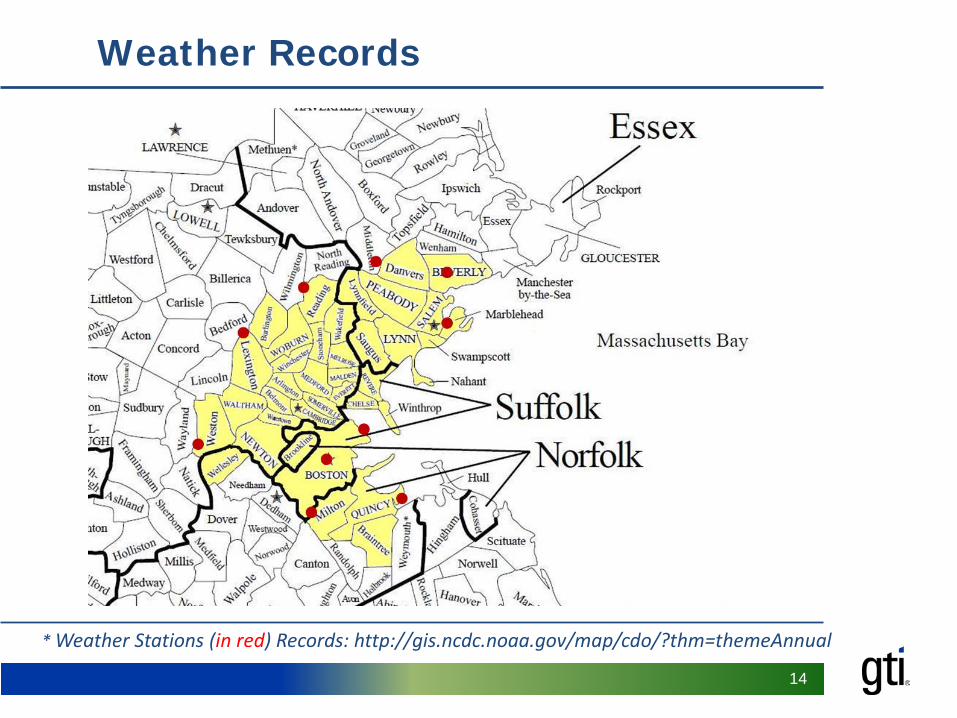
The project reviewed the cast iron pipeline inventory in the eastern region of MA.

This region included towns in four counties (Essex, Middlesex, Suffolk, and Norfolk) and had a total of 2,258 miles of CI main, which is about 20% of the CI inventory in the gas distribution system in New England and NY.

Investigated leak-database records during the winter months in the period from 2001 to 2012.

6

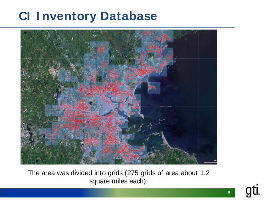
CI Inventory Database

The area was divided into grids (275 grids of area about 1.2 square miles each).

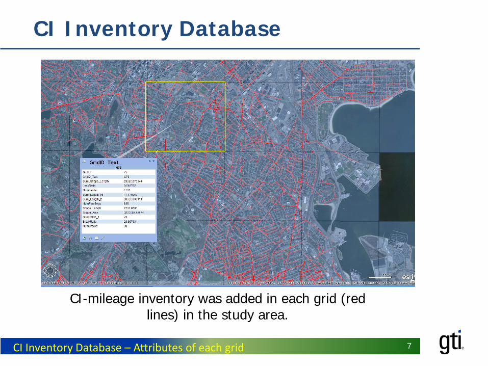
7 CI Inventory Database – Attributes of each grid

CI Inventory Database

CI-mileage inventory was added in each grid (red lines) in the study area.

8 CI- Leak Database (2001-2012)

CI Leak Database

CI leak inventory was added in each grid (yellow dots) in the study area.

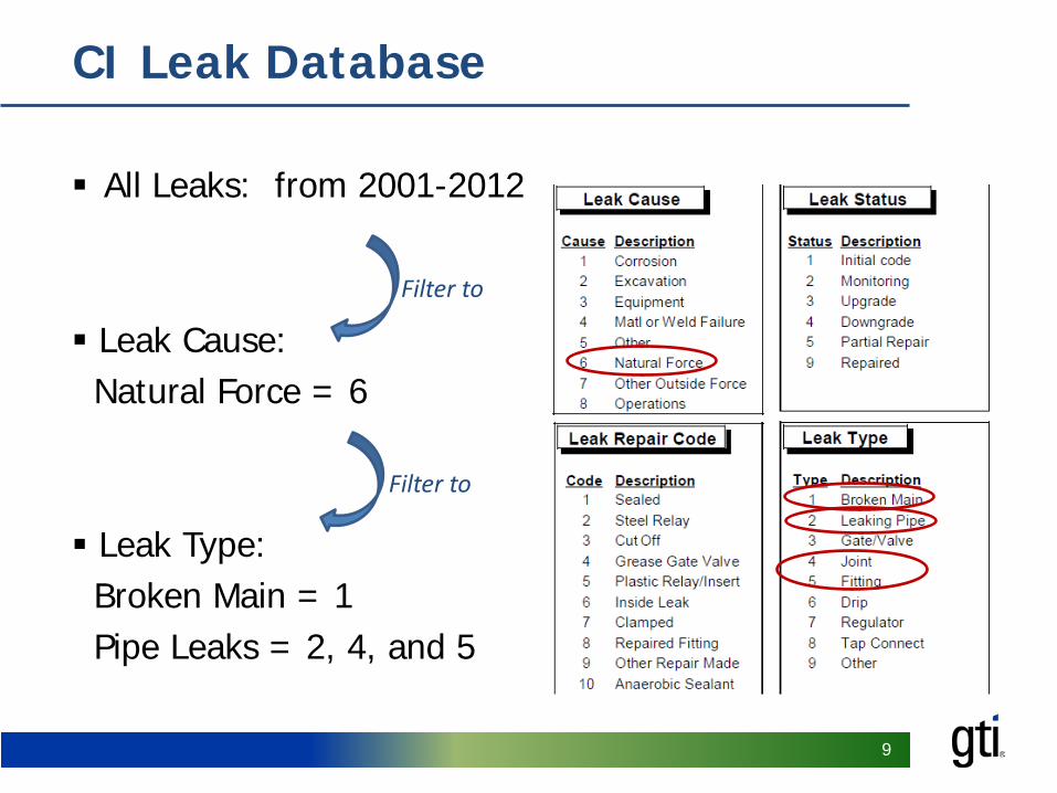
9

All Leaks: from 2001-2012 Leak Cause: Natural Force = 6 Leak Type: Broken Main = 1 Pipe Leaks = 2, 4, and 5

CI Leak Database

Filter to

Filter to

10

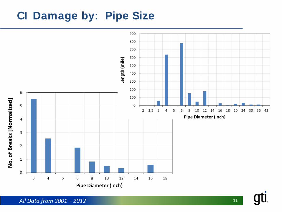
CI Leaks by: Pipe Size

Leak Type Data from 2001 - 2012 Histograms, Program: Statistica Note: Data in graph is not normalized with length of CI for each pipe size

11 All Data from 2001 – 2012

No.

of B

reak

s [N

orm

alize

d]

CI Damage by: Pipe Size

12

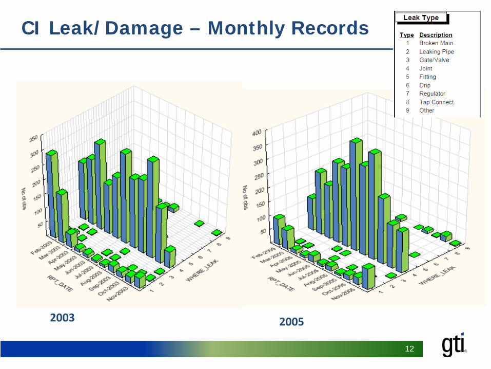
CI Leak/Damage – Monthly Records

2003 2005

13

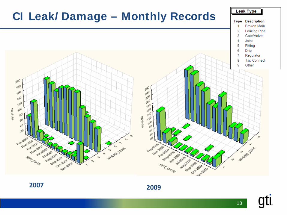
2007 2009

CI Leak/Damage – Monthly Records

14

* Weather Stations (in red) Records: http://gis.ncdc.noaa.gov/map/cdo/?thm=themeAnnual

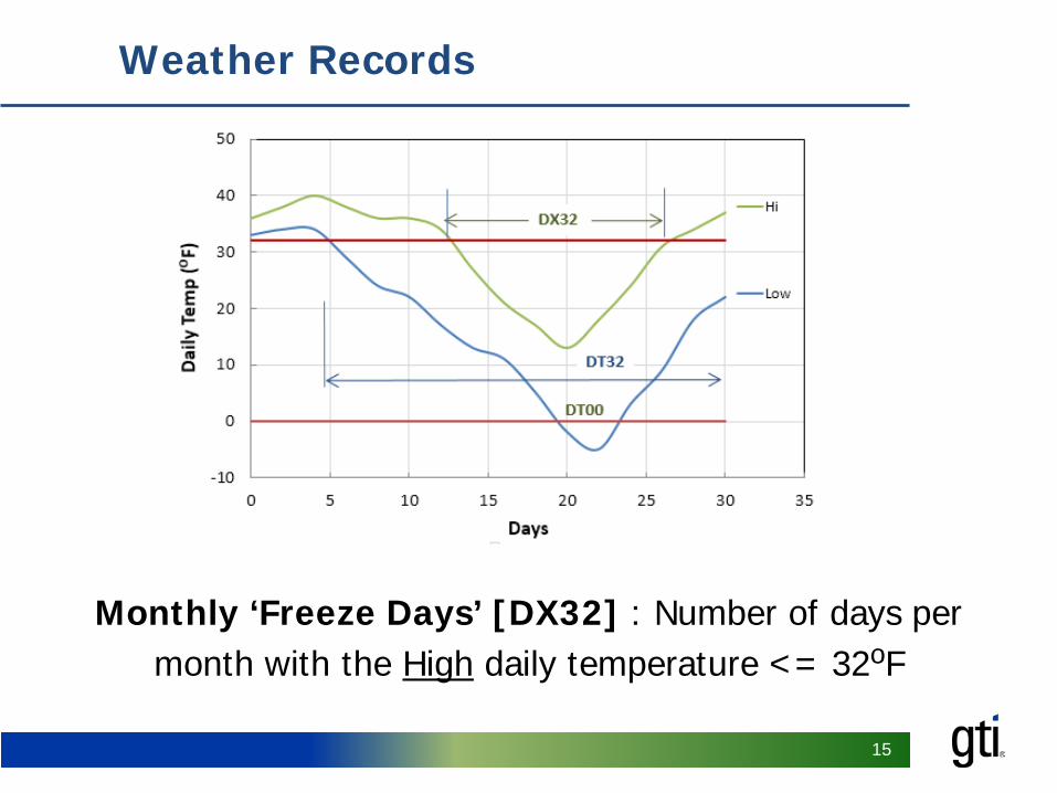
Weather Records

15

Monthly ‘Freeze Days’ [DX32] : Number of days per month with the High daily temperature <= 32oF

Weather Records

16

Monthly ‘Freeze Days’ [DX32] : Number of days per month with the High daily temperature <= 32oF

Weather Records

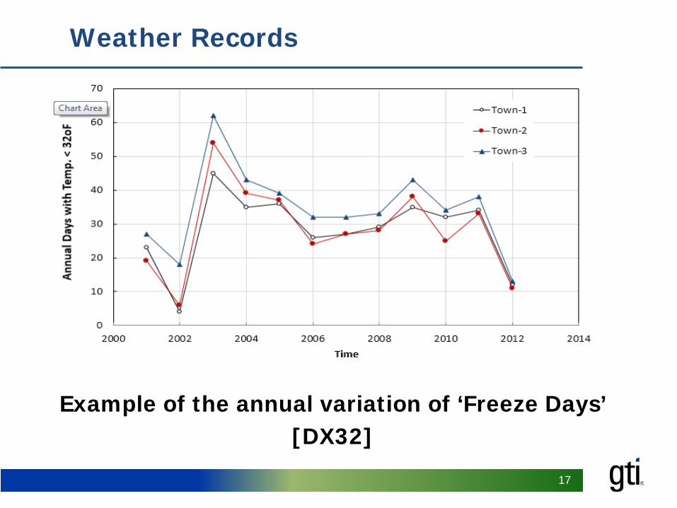
17

Weather Records

Example of the annual variation of ‘Freeze Days’ [DX32]

18

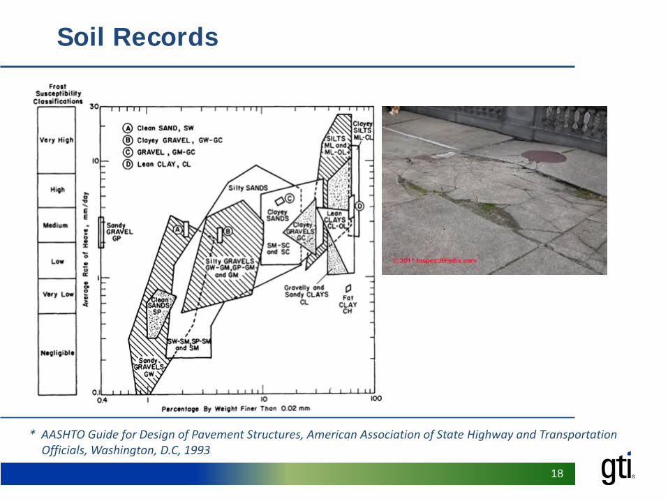
* AASHTO Guide for Design of Pavement Structures, American Association of State Highway and Transportation Officials, Washington, D.C, 1993

Soil Records

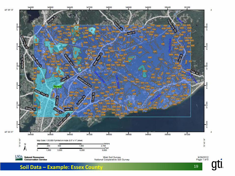
19 Soil Data – Example: Essex County

20

Soil Records

21

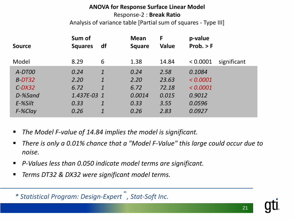
* Statistical Program: Design-Expert®, Stat-Soft Inc.

ANOVA for Response Surface Linear Model Response-2 : Break Ratio

Analysis of variance table [Partial sum of squares - Type III]

Sum of Mean F p-value Source Squares df Square Value Prob. > F Model 8.29 6 1.38 14.84 < 0.0001 significant A-DT00 0.24 1 0.24 2.58 0.1084 B-DT32 2.20 1 2.20 23.63 < 0.0001 C-DX32 6.72 1 6.72 72.18 < 0.0001 D-%Sand 1.437E-03 1 0.0014 0.015 0.9012 E-%Silt 0.33 1 0.33 3.55 0.0596 F-%Clay 0.26 1 0.26 2.83 0.0927

The Model F-value of 14.84 implies the model is significant. There is only a 0.01% chance that a "Model F-Value" this large could occur due to

noise. P-Values less than 0.050 indicate model terms are significant. Terms DT32 & DX32 were significant model terms.

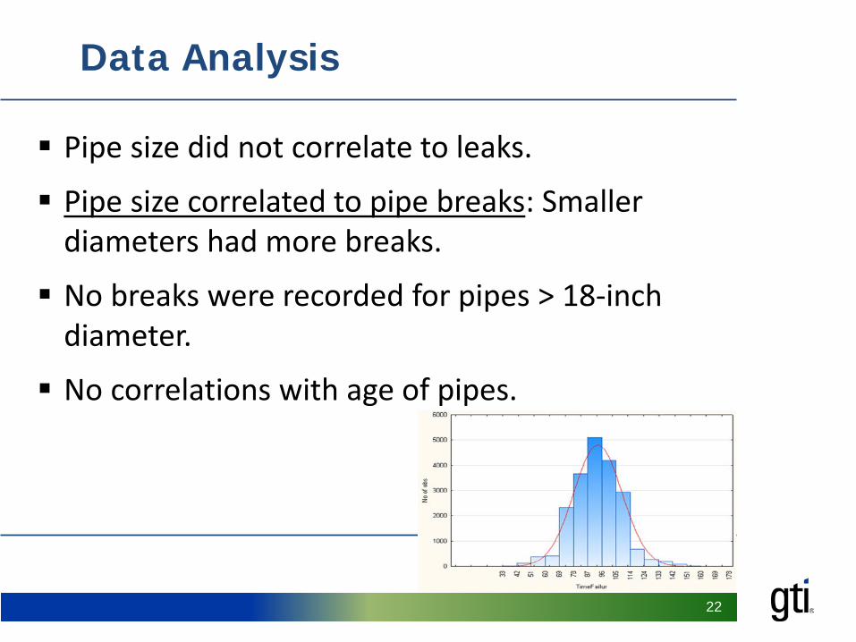
22

Pipe size did not correlate to leaks.

Pipe size correlated to pipe breaks: Smaller diameters had more breaks.

No breaks were recorded for pipes > 18-inch diameter.

No correlations with age of pipes.

Data Analysis

23

Soil properties were obtained from the ‘Web Soil Survey’ database of the U.S. DOA.

Soil with high silt and clayey-silt contents are more susceptible to freeze and heave. However, soil data could not be used as a ‘trigger’ to predict pipe damage or initiate winter surveillance.

Some of the factors are: (a) soil variations make it difficult to estimate soil-frost susceptibility, and (b) backfill around the pipes in the urban areas differs from native soils listed in the database.

Data Analysis

24

Freeze-Days: Number of days per month with the High-Daily temperature <= 32oF.

Freeze Days’ relates to the other commonly used term:

‘Frost Degree Days’, which is: Number of days with the high-daily temperature T <= 32oF multiplied by (32-

T)oF].

The relationship between ‘Freeze-Days’ and pipe damage records was plotted in the following slides.

Data Analysis

25

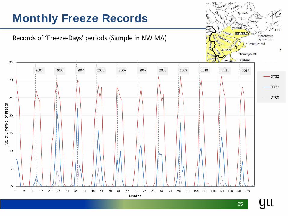
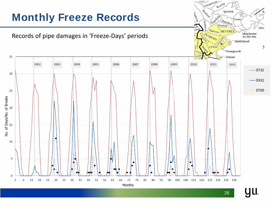
Monthly Freeze Records

Records of ‘Freeze-Days’ periods (Sample in NW MA)

26

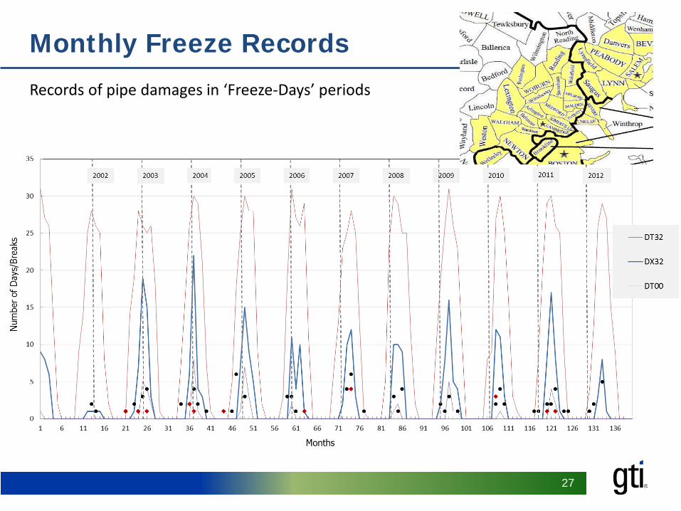
Monthly Freeze Records

Records of pipe damages in ‘Freeze-Days’ periods

27

Monthly Freeze Records

Records of pipe damages in ‘Freeze-Days’ periods

28

Conclusions

The correlation between the ‘Freeze-Days’ and pipe damage was evaluated in 18 towns in the NE. Most of the winter pipe damages (90%) occurred after 5 days accumulation of the Freeze-Days.

This correlation can be used to establish a criterion for initiating winter patrols and to optimize the probabilities of detecting winter damage.

Soil freeze-depth varies widely and is highly dependent on soil type, moisture condition, and type and thickness of the pavement cover. This makes it difficult to have a representative soil freeze-depth for the whole region.

29

Conclusions

‘Freeze-Days’ provides a better correlation than using ‘Average Daily Temperature’ to correlate to CI.

Utilities may use the weather data in their service areas to establish similar winter surveillance plans.

The following slides provide a suggested procedure for the scheduling winter patrol as an illustration of the approach to implement weather data.

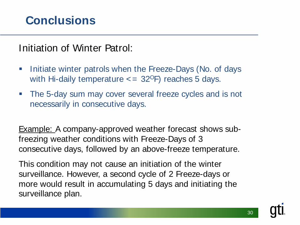
30

Initiation of Winter Patrol: Initiate winter patrols when the Freeze-Days (No. of days

with Hi-daily temperature <= 32OF) reaches 5 days.

The 5-day sum may cover several freeze cycles and is not necessarily in consecutive days.

Example: A company-approved weather forecast shows sub-freezing weather conditions with Freeze-Days of 3 consecutive days, followed by an above-freeze temperature.

This condition may not cause an initiation of the winter surveillance. However, a second cycle of 2 Freeze-days or more would result in accumulating 5 days and initiating the surveillance plan.

Conclusions

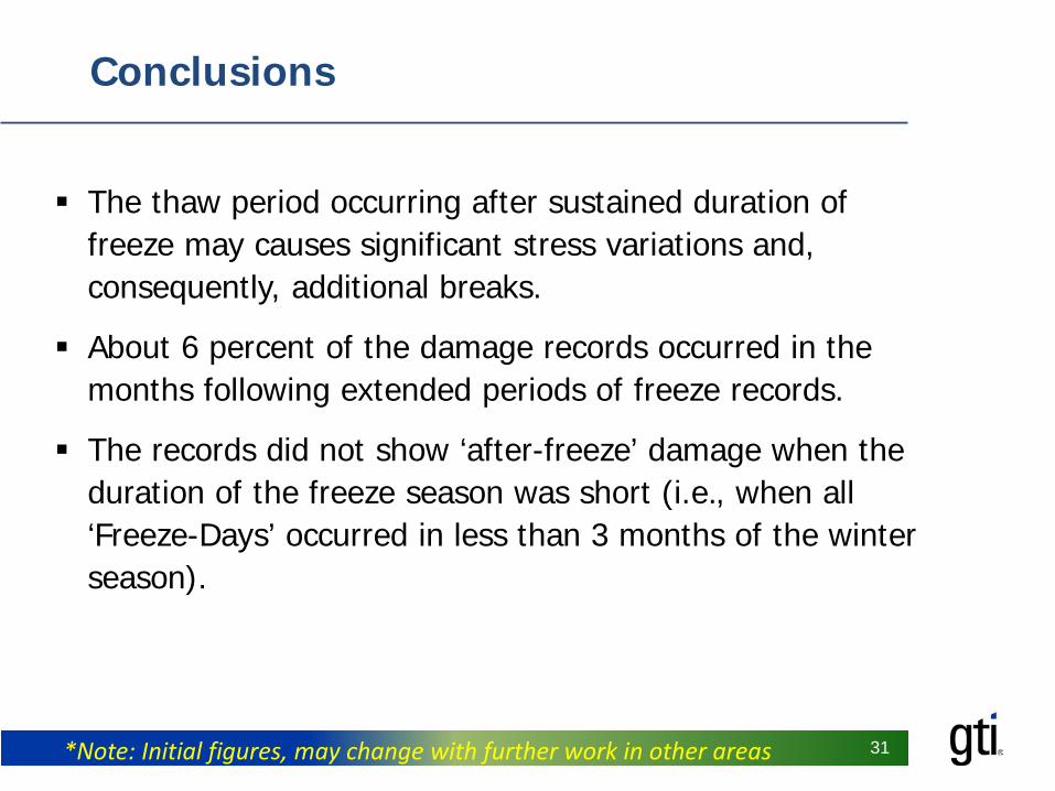
31 *Note: Initial figures, may change with further work in other areas

The thaw period occurring after sustained duration of freeze may causes significant stress variations and, consequently, additional breaks.

About 6 percent of the damage records occurred in the months following extended periods of freeze records.

The records did not show ‘after-freeze’ damage when the duration of the freeze season was short (i.e., when all ‘Freeze-Days’ occurred in less than 3 months of the winter season).

Conclusions

32

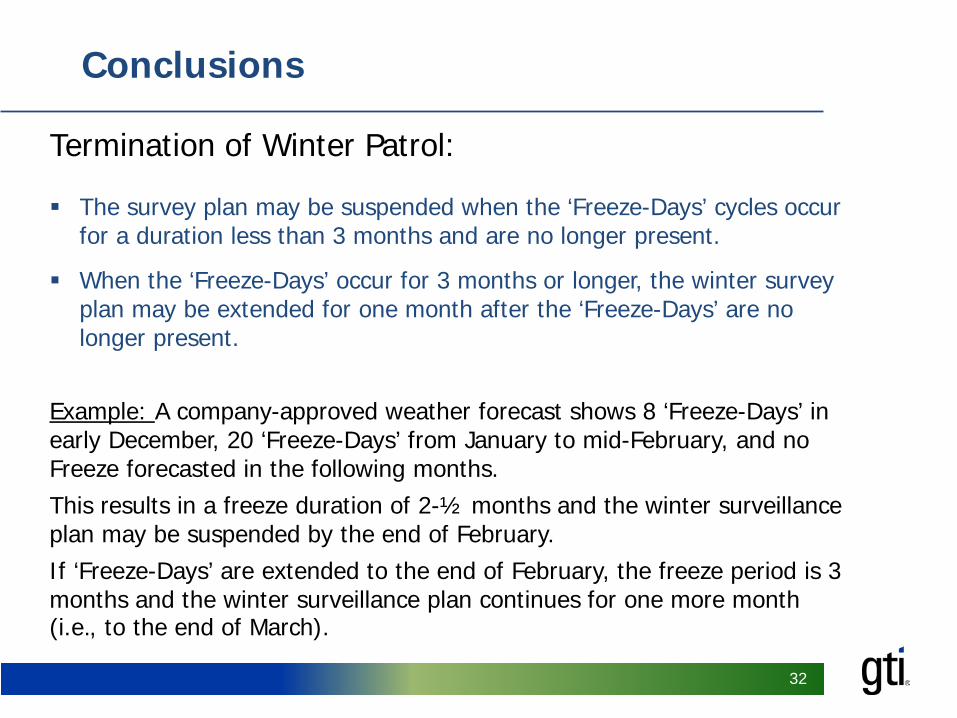
Termination of Winter Patrol: The survey plan may be suspended when the ‘Freeze-Days’ cycles occur

for a duration less than 3 months and are no longer present.

When the ‘Freeze-Days’ occur for 3 months or longer, the winter survey plan may be extended for one month after the ‘Freeze-Days’ are no longer present.

Example: A company-approved weather forecast shows 8 ‘Freeze-Days’ in early December, 20 ‘Freeze-Days’ from January to mid-February, and no Freeze forecasted in the following months. This results in a freeze duration of 2-½ months and the winter surveillance plan may be suspended by the end of February. If ‘Freeze-Days’ are extended to the end of February, the freeze period is 3 months and the winter surveillance plan continues for one more month (i.e., to the end of March).

Conclusions

33

Tackling Important Energy Challenges and Creating Value for Customers in the Global Marketplace

Paul Armstrong Director Business Development, GTI paul.armstrong@gastechnology.org 781-449-1141 www.gastechnology.org

@gastechnology