assessing the impact of us macroeconomic policies and inflation rates on the australian economy

Assessing the Impact of US Macroeconomic Policies and Inflation Rates on the Australian

Economy*

RICHARD C.K. BURDEKIN Chremont McKenna College

and Chremont Graduute School USA

A three-equation system is specified with Australian monetary buse growth, the domestic budget deficit and the domestic inflation rate as dependent variables Lugged vulues of these three variables and their US counterparts are entered us erplnnutory variables in each equation Results for 1967-83 suggest u possible effect of hgged US monetary base growth on Australian monetary b w growth plus a positive direct impact of US inflution on Austrulian inflrrtion

I Introduction In the small economy under fixed exchange rates,

macroeconomic policies and inflation rates are likely to be particularly vulnerable to the international transmission of economic disturbances from the rest of the world. Unlike almost all other major developed countries, Australia remained on fixed exchange rates after the breakdown of Bretton Woods and the Australian dollar was not floated until December 1983. Using US variables to reflect 'rest of the world' effects, this study seeks to assess the interrelationships between domestic and US monetary policy, fiscal policy and inflation for Australia over the 1967-83 period. At the same time, allowance is made for a possible structural break corresponding to the switch to a 'crawling peg' exchange rate regime in September 1974. occurring as it did in conjunction with the worldwide adoption of more freely floating exchange rates around that time. A three-equation model is employed in the analysis, with domestic monetary base growth, the domestic budget deficit *The author is grateful for helpful comments and suggestions from Paul Burkett. Mark Wohar and an anonymous referee.

and the domestic inflation rate as dependent variables. The results provide some evidence that US monetary base growth may significantly influence Australian monetary base growth. A positive impact of US inflation on Australian inflation also emerges, and there is some suggestion of additional negative effects on Australian monetary base growth and budget deficits. There is no evidence of any impact arising from US budget deficits.

I! A SimpkfEd Two-Country Setting Under fixed exchange rates and with the United

States as the reserve currency country. domestic money growth in the small economy will tend to be automatically linked to US money growth via the balance of payments. Here, an increase in US money growth leads to an excess demand for goods and capital in the United States and to a corresponding outflow of funds from the US economy as this excess demand is translated into flows of imports. Such flows of US dollars abroad require the foreign central bank to purchase US dollars with foreign assets in order to maintain the fixed exchange rate, with an increase in the foreign monetary base being the means of funding these

16

1992 ASSESSING THE IMPACT OF US MACROECONOMIC WLlCIES 17

purchases.' Another channel of transmission is suggested by the monetary approach to the balance of payments, whereby the determination of tradeable goods prices according to the law of one price directly links domestic inflation to foreign inflation. In this way, foreign money growth could influence domestic inflation through its effect on foreign and/or world inflation in addition to that on domestic money growth.

More formally, under purchasing power parity, we can write

p = p ' + e ( 1 )

where p is the rate of domestic inflation in the small economy, p' is the rate of inflation in the United States (as the reserve currency country), and e is the percentage change in the exchange rate.

Following Darby and Lothian (1989). let this equation be combined with a money demand function of the form:

IW' = uy. i, u) + p (2)

where mJ is the percentage growth rate of nominal money demand, y is the percentage growth rate of real income, i is the rate of change of the nominal interest rate, and u is a portmanteau variable capturing other determinants of money demand.

In this stylized setting, equality between the rate of money supply growth (m) and money demand, together with the zero value for e implied under the fixed exchange rate case yields:

m = U y , i u) +p'. (3)

In this way, higher inflation in the United States will, cereris paribus, be expected to raise the equilibrium rate of domestic monetary expansion via the increase in the domestic inflation rate and

I In principle, the monetary base and money stock in the small economy need not increase if international reserve flows could be successfully sterilized by the central bank. Laney and Willett's (1982) examination of sterilization coefficient estimates suggests, however, that international reserve increases did remain the predominant cause of monetary expansion in Australia, even though a stronger role for domestic factors was indicated for a number of the other countria examined.

associated rise in W. Hence, effects of higher rates of monetary expansion in the reserve currency country would be felt, not only directly as the central bank in the small economy (in order to maintain the fixed exchange rate) funds purchases of US dollars with an increase in domestic credit, but also indirectly to the extent that US inflation itself increases with higher rates of US money growth.

There is also scope for effects of US fiscal policy following from any impact a higher US budget deficit, say. may have on world inflation and/or world interest rates. If the dominate effect were on interest rates. then the resulting decrease in money demand would imply a reduced rate of monetary expansion in the small economy from equation 3. Finally, impacts of the US variables on fiscal policy in the small economy could follow from any tendency for the domestic budget deficit to rise with the higher inflation rates implied by higher US inflation and/or more expansionary US monetary and fiscal policies. That is, any such upward pressure on world and domestic prices suggests that, if planned provision of government goods and services is to be held constant in real terms, some increases in government purchases in nominal terms will be required-thus providing for an automatic merchanism that may tend to raise the domestic budget deficit in the absence of any discretionary policy move.?

The extent to which the small economy remains vulnerable to US influences under a floating regime is more questionable. Allowance for a floating exchange rate in the simple three-equation set-up laid out above would leave the small economy's inflation rate determined by the domestic rate of excess money growth alone. At the same time, there is scope for setting domestic money supply growth independently so long as the central bank is willing to accept the consequences of, say. exchange rate appreciation in the face of a policy that lowers the domestic inflation rate below that level prevailing abroad.

In practice, however, attempts to maintain exchange-rate and interest-rate stability can

2 Higher inflation may also be associated with political prasurc for increased government outlay arising from groups seeking to make good losses on implicit contracts upset by unanticipated inflation. In obtaining cross- sectional evidence on inflation as a causal influence on government spending. Opler (1988, p. 333) finds that, for the sample ofcountries adhering to the Bretton Woods agreement prior to the early 1970s. 'the relationship between inflation and government growth remained even when inflation was imported from the United States'.

18 ECONOMIC RECORD MARCH

account for a continued channel of monetary transmission from the United States. In the Australian case. for example, Marsden and Jones (1988) describe how central bank interventions to moderate the rate of depreciation of the Australian dollar have, at least in the period since August 1986, led to a considerable 'dirtying' of the float- with the Reserve Bank intervening in the market by selling foreign exchange and buying domestic currency so as to strengthen the Australian dollar.' Such policy rules involving direct exchange rate manipulation must, by their very nature, limit the degree of possible insulation against externally generated inflation (see Pitchford and Vousden. 1987, for formal analysis of this issue)!

Nevertheless, the radical nature of the change in strucrure associated with a move toward even a 'dirty' float is undeniable. Indeed. Darby and Lothian (1989) consider that, although short-run inter-country linkages may have persisted in those countries adopting floating exchange rates after 1973. so long as the associated interest-rate and exchange-targets feature sufficient flexibility the degree of long-run monetary independence may still be substantial. Darby and Lothian in fact obtain evidence on the cross-country variability of inflation, money growth and interest rates supporting such enhanced long-run independence in the period following the advent of flexible exchange rates.

In the Australian case, the degree to which the domestic economy has remained vulnerable to continued international transmission of inflation after the December 1983 float of the domestic currency requires more post-I983 data than is currently available. However, the evidence presented below regarding the pre-float period does nevertheless provide a possible yardstick by which the later experience may be compared and, in indicating the specific effects emanating from the United States which have been of most importance

Empirical evidence of such intervention bchaviour, or 'leaning against the wind', is obtained by Hopkins (1988). Moreover, her results suggest that intervention activity actually increased in the period following the December 1983 floating of the Australian dollar. ' That is not to say that complae insulation from

external inflation will necessarily be attained even under a freely floating exchange rate. Pitchford (1985). for example, points to necessary conditions for complete insulation that include. not only perfect foresight, but also an operative Fisher effect in the foreign country together with a uniform foreign inflation rate that involves all foreign nominal magnitudes increasing at the same rate.

in the past, may well point to influences that are potentially also relevant in the current mode of dirty floating.

III Revwus Studies of the Transmkwn of US Poky Variables

A causal role for US monetary base growth in determining 'world' money stock and inflation rates in the years prior to the breakdown of Bretton Woods is certainly suggested in the review provided by Parkin (19771.5 A subsequent analysis of the fixed exchange rate era by Feige and Johannes ( 19821, however, obtains some apparently contrary evidence in that, for the six countries included in the study, foreign monetary growth and inflation rates are not found to be systematically related to growth in the US money supply. Meanwhile, Sheehan ( 1987) finds that US and foreign money growth generally were related under fixed exchange rates, while a more limited effect of US money growth is observed under floating exchange rates where the null hypothesis of independence could be rejected only for Canada and Japan.6.

The particular influence of US monetary growth-as measured under the M- I definition of the money supply-on Australian monetary growth has previously been examined by Layton (I 983, 1986). Using quarterly data from I959(3)- I978(4), Layton finds that US money growth leads Australian money growth with a lag of approximately 18 months. This finding holds both in a bivariate context and also when Australian income growth is included as an additional right- hand-side variable in the Australian money growth equation.

The inferences that can be drawn from Layton's analysis are, however, limited by the exclusive focus on the effect of US money growth on domestic money growth. Possible influences of US money growth on domestic fiscal policy and inflation rates, for example, as suggested in the preceding section, would also be of interest. Moreover, incorporating US influences on, say, domestic money growth to the exclusion of any

In this context, the 'world' is the aggregate of countries which maintained a fixed exchange rate with the US dollar-and full convertability-in the 1958-7 I period examined by Parkin.

Substantial US influences on the four largest European economies of France, Italy, the United Kingdom and West Germany are, however, found to endure across both fixed and floating exchange rate periods in Burdckin (1989).

1992 ASSESSING THE IMPACT OF US MACROECONOMIC POLICIES 19

domestic interactions between monetary policy, fiscal policy and inflation suggests a danger of omitted variable bias. For example, in allowing for such domestic interactions in the United States, Ahking and Miller (1985) have modelled money, deficits and inflation as a trivariate autoregressive process. finding all three to be causally related (in the sense of Granger's temporal causality, where the past and present can cause the future. but the future cannot cause the past) for the 1950s and 1970s.

Effects of US monetary policy may themselves be transmitted not only directly but also indirectly via the impact of higher rates of US monetary expansion on US-and hence world-inflation. This suggests the desirability for testing for effects of US inflation in order to obtain a fuller assessment of the impact of US monetary policy on the small economy. Finally. there is the question of US fiscal policy effects, for which the existing evidence is rather mixed. On the one hand, Evans (1986) finds no impact of the US budget deficit on the exchange value of the dollar, while Memck and Saunders ( 1986) also find no affect of US fiscal policy on international real interest rates. At the same time, significant effects of US government spending shocks on both exchange rates and interest rates are suggested by Masson and Blundell- Wignall ( 1985).

IV The hpitical Procedure The present study seeks to assess the influence

of US monetary policy within the more general context of a three-equation system that, following initial estimation by ordinary least squares (OLS). is then estimated simultaneously to take advantage of the efficiency gains arising from the iterative Zellner-Aitken procedure. The sample (comprising quarterly data) is extended through December 1983 to include all observations available prior to the floating of the Australian dollar at the end of that year. The analysis foduses on domestic and US monetary base growth due to the monetary base reflecting the stance of monetary policy, and the outcome of central bank open-market operations, more directly than does M- 1.'

The Australian budget deficit as a ratio to GNP ( D E B and domestic inflation rate (DP), together

Naturally. the monetary base has less applicability as a measure of policy stance in a small economy owing to the very international influences that are the subject of this paper. See Barry (1978) for further analysis on this point.

with domestic monetary base growth (DMB), comprise the full set of endogenous variables. Lagged values of US monetary base growth (USUB), the US budget deficit divided by GNP (USDEF) and the US inflation rate (USDP) along with lagged values of each of the Australian variables are entered on the right-hand side of each equation.8 As such, the chosen methodology permits the importance of the US effects hypothesized in Section 2 to be assessed in conjunction with the role played by domestic in teractions.Y

In view of International Monetary Fund (IMF) data on the Australian budget deficit not being available prior to 1965( 1). the estimation period- after allowance for lags-is set from 1967( I)- 1983(4). It is assumed, for simplicity, that the dependent variables are linearly related to the right-hand-side variables. Given that information lags make within-period responses to innovations in the explanatory variables unl ike ly . contemporaneous terms are excluded and the minimum lag length is assumed to be one quarter.

We have the following system of equations that is 10 be estimated for Australia:

D M B = ~ ~ + u ~ ( L ) D M E + u ? ~ U D U ; + U ~ ( L ) D ~ ~ ~ , ( ~ U S M B (4) +u~(UUSDEF+U~UUSDP+U,

DEF=hi,+bi(L)DMB+h(L,DEFfb,(L)DP+h,(L)USMB ( 5 ) + bs(UUSDEF+bdUUSDptV,

DP;c,,+r,(L)DMB+c~L)Dff~c$L)DP+c,(L)USMB (6) +cS(L)USDEF+C~UUSDP+W~

where DUB is the rate of growth of the domestic monetary base, DEF is the domestic budget deficit divided by domestic GNP, DP is the rate of growth of the domestic consumer price index, USMB is the rate of growth of the US monetary base, USDEF is the US budget deficit divided by US GNP, USDP is the rate of growth of the US consumer price index,

" Evidence that the US inflation rate is itself exogenous with respect to the rest of the world is provided by Darby (I98 I).

Here. the effect of other variables, such as i and y in Section 11. is (by necessity. given the limited number of observations available) taken to be subsumed in the reduced form responses to the monetary. fiscal and inflation variables appearing on the right-hand side of the equations.


(L) is the lag operator, u, v, and w, re error terms.

The question of the lag lengths that should be applied to each variable is addressed by first estimating each equation separately by OLS with the lags on each variable set at a maximum of eight quarters. Akaike's (1970) Final Prediction Error (FPE) criterion is then applied as the lags on each right-hand-side variable are successively reduced from eight to zero, holding the lag length on the others at the maximum. While this at first involves estimating 52 parameters with 68 observations, it should be pointed out that, by way of correcting for the large starting number of right- hand-side variables, the initial FPE-selected lags were themselves used as the maxima in a second application of the procedure. None of the final specifications derived from this lag reduction process has any more than 20 parameters to be estimated over the 68 observations.

The FPE criterion itself is an appealing decision rule in that i t trades off the risk due to bias when a shorter lag length is selected against risk due to increase in variance when a higher order is chosen. Furthermore, the criterion allows the effect of each variable to be felt at a different lag length- selection of which is dictated by the minimum value of the statistic

T+(L+K+ I -d) FpE= T-(LSK+I-d) ' T d=O,I.. . .,L (7)

where T is the number of observations, L is an arbitrarily chosen maximum lag length, K is the number of explanatory variables, d represents the lag length restrictions imposed, and RSSL-,, is the residual sum of squares from the regression with d lag restrictions imposed.

After applying the FPE criterion to each equation and deleting those variables for which the criterion selects a lag length of zero, OLS estimation of the resulting final specifications is followed by joint-estimation of the three-equation system by generalized least squares (GLS), using the maximum likelihood procedure provided by the Time Series Processor (TSP) software package. In this way, allowance is made for cross-equation correlation of disturbances as suggested by Zcllner (1962). Certainly, to the extent that each of the dependent variables in the equations estimated for Australia is vulnerable to the same external shocks-that is, contemporaneous, stochastic disturbances not captured by the available set of

right-hand-side variables-the appeal to potential cross-correlation of the error terms is seemingly well-justified on a priori grounds.

V Estimation Results for Australia The results for the OLS and GLS estimations

of the final specifications for the monetary base, budget deficit and inflation rate are presented in Tables 1-3. Results for the sums of the lags on each variable and for tests of the overall significance levels for each set of coefficients are presented in Table 4. In the case of the OLS estimation, the reported F statistics test the joint significance of the coefficients comprising the sum of the lags on each variable. For the GLS results, likelihood ratio tests are applied by re-estimating the system of equations after excluding all lagged values of the variable from the individual equation in question.1" Here, comparison of the OLS and GLS results reveals that, while the values of the individual coefficients and coefficient sums appear quite robust to the application of the GLS procedure, the t statistics are almost uniformly higher and the overall significance levels for the sums of the lags are also improved under GLS.II In the GLS case, all of the variables are significant at the I per cent level except for USDP in the monetary base equation-itself significant only at the 10 per cent level.

It is important to consider, however, whether contemporaneous correlation of the error terms across equations is complicated by serial correlation of the errors within the individual equations themselves. Here, in light of the complications in testing for autocorrelation under GLS estimation, attention is focused on residuals from the OLS regressions. Now, the Durbin- Watson statistics reported in Tables 1-3 themselves test only for first-order serial correlation and, moreover, are biased toward 2 in the deficit and inflation equations because lagged dependent variables appear on the right-hand side. In this case, an alternative testing procedure-developed by

1'' The likelihood ratio is given by two times the difference between the restricted and unrestricted log likelihood. This provides a test statistic that is distributed as a x' stalistic with degrees of freedom equal to the number of restrictions imposed-that is, the number of lags on the variable being excluded.

' 1 Although it should be pointed out that, strictly speaking, the test statistics obtained for the GLS case are themselves valid only asymptotically-see Rothenberg ( I 984) on the conditions for approximate normality of the GLS estimates.


TABLE I

Monetary BaK Equation

Dependent Variable DMB Sample I967:l- 1983:4

GLS Results OLS Results

Coefficient t Statistic Coefficient t Statistic Constant 0.099 (4.78) 0.105 (4.26) DR- I ) 0.795 (1.45) 0.804 ( I .24) DR-2) - I .389 (-2.45) - I .446 (-2.15) DR-3) 0.088 (0.16) -0.003 (-0.004) DR-4) I .022 (1.91) I .073 ( I .68) DR-5) 0. I07 (0.20) 0.249 (0.38) DR-6) - I .279 (-2.43) - I .303 (-2.05) DR-7) -0.6 I6 (- 1.21) -0.299 (-0.49) DR-8) I .479 (3.01) I .227 (2.08) USMB( - I ) -0.826 (-2.88) -0.894 (-2.58) USMB( - 2 ) -0.235 (-0.75) -0.305 (-0.80)

USMB( -4 ) -0.445 (- 1.36) -0.507 (-1.28) USMB( - 5 ) 0.108 (0.33) 0.032 (-0.08)

USMB( - 3 ) 0.088 (0.27) 0. I23 (0.3 I )

IISMB( - 6) 1.179 (3.39) 1.304 (3.09) USMB( - 7 ) 0.443 ( 1.37) 0.5 3 7 ( I .38) USDR- I ) -1.056 (- 1.81) -1.138 ( - I .64)

Summary Statistics for OLS Results R2=0.54; 0=0.037; Flo,,p5.21; DW=1.88 where a is the standard error of the regression. and DW is the Durbin- Watson statistic.

Note: As in each subsequent case. three seasonal dummies were included in the regression alongside the variables listed in the table.

TABLE 2

Deficit Equation

Dependent Variable DEF Sample 1967: I - I983:4


Coefficient I Statistic Coefficient t Statistic Constant 0.009 ( I .97) 0.010 (2.00) DMB(- I ) -0.0 I9 (- I .53) -0.015 (-1.01) DMB(-2) -0.033 (-2.47) -0.036 (-2.25) DMB( -3 ) -0.009 (-0.7 I ) -0.0 10 (-0.63) DMB(-4) -0.037 (-2.88) -0.040 (-2.65) DEF(- I ) 0.252 (2.34) 0.216 (1.72) DER-2) -0.002 (-0.02) 0.036 (0.28)

DER-4) 0.467 (4.29) 0.462 (3.62) 09- 1) 0.073 (1.10) 0.066 (0.86)

DR-3) 0.195 (3.48) 0.209 (3.18)

DEF(-3) -0.034 (-0.29) -0.04 I (-0.30)

DS-2) 0.006 (0.1 I) -0.004 (-0.05)

DR-4) -0.077 (-I .29) -0.063 (-0.89) USDS- I ) -0. I98 (-3.10) -0.202 (-2.73)

Summary Statistics for OLS Results %0.95; a=O.o04; FIb~I=73.98; DW=1.90


TABLE 3

lnfloiion Equation

Dependent Variable DP Sample 1967:l-1983:4


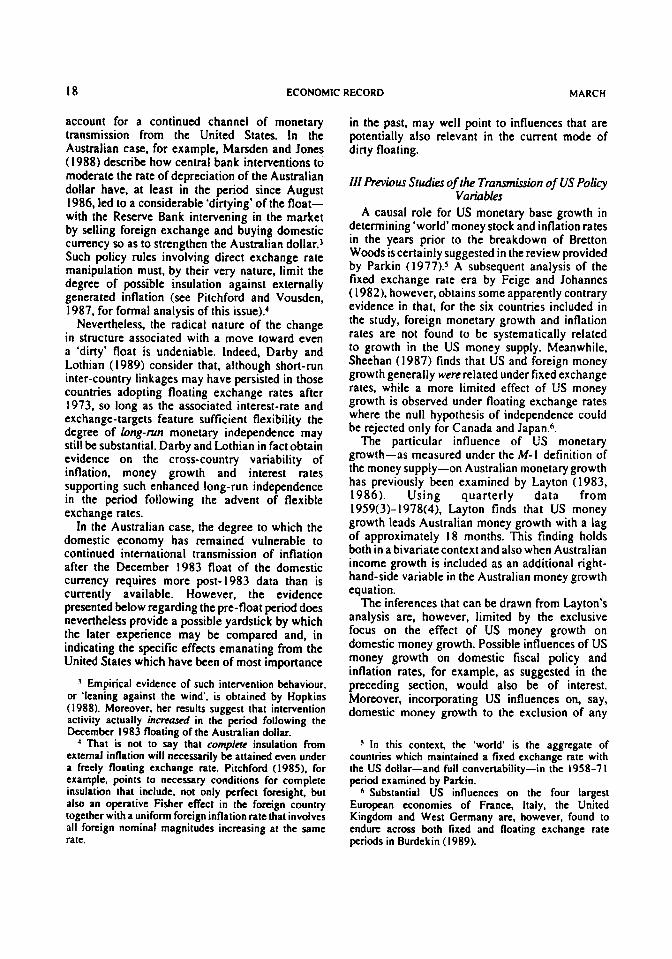
Coemcient I Statistic Coefficient f Statistic Constani 0.0 I6 ( 1.86) 0.0 I9 (1.77) DMm- I j 0.077 (3.61) 0.082 (3.22)

DMN-3) 0.006 (0.28) 0.005 (0.19) DMBI-4) 0.058 (2.78) 0.056 (2.28) D r n - I ) 0.206 (1.12) 0.193 (0.88) DER-2) -0.539 (-2.85) -0.48 I (-2.14) DER-3) 0.574 (2.71) 0.569 (2.26)

DER-5) -0.607 (-3.13) -0.693 (-2.97) DER-6) 0.597 (2.94) 0.573 (2.34)

DM&-2) -0.043 (- I .89) -0.048 (- I .76)

DER-4) -0.080 (-0.37) -0.0 19 (-0.07)

DER-7) -0.053 (-0.25) -0.040 (-0.16) DER-8) -0.404 (-2.09) -0.456 (- I .95) D U - I ) 0.336 (3.2 I ) 0.320 (2.59) DU-2) 0.3 I5 (3.18) 0.332 (2.83) USDR- I ) 0.395 (3.67) 0.41 I (3.23)

Summary Statistics for OLS Results k 0 . 6 9 ; 0=0.007; F14,p'8.5 I ; DW=2.08

TABLE 4

MLS for rhe Sums of rhe Lugs


Number Sum Li kelihood Sum

Variable L g s Lags Statistic Lags Statistic of of Ratio Test of F-Test

Monetary DP Base Equation USMB

USDP

Deficit DMB Equation DEF

DP USDP

Inflation DMB Equation DEF

DP USDP

8 7 I

0.207 0.3 12 - I .056

-0.098 0.683 0.197

-0.198

0.098 -0.306 0.65 1 0.395

~ 4 ~ 2 2 . 5 8 , xf= 18.72. xf=3. I2***

xl=16.79* +29.35* xf= I7.84* xf=8.9 I

x3=22.00* +26.6 1 x3=4 I .45* xf= 12.01*

0.302 0.290

-1.138

-0.101 0.673 0.208

-0.202

0.095 -0.354 0.652 0.41 I

NOW *. ** and *** denote significance at the I per cent, 5 per cent and 10 per cen; levels. respectively. The likelihood ratio and F-test statistics apply to the o w d significance of the respective lag distributions.


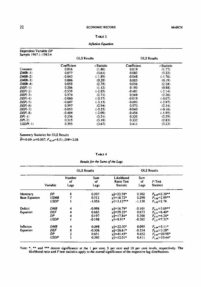
TABLE 5

Bnusch-Godfrey Tern for Serial Cotrelath of the Residuals in the OLS Rcgmciom

x 2 Test Siaricrics Monetary

Equation Equation Equation Values Lag

Order

1 0.27 0.8 I 0.37 x+3.84

3 2.06 3.76 4.64 x+7.82

5 6.77 7.25 5.5 I xj= I 1.07 6 7.44 8.32 5.83 x2=12.59 7 7.85 11.29 5.23 x3= 14.07

9 10.73 11.55 10.55 xj=16.92

Base Deficit Inflation 5% Critical

2 2.09 2.03 4.8 I x3=5.99

4 6.30 7.4 I 5.63 xt=9.49

8 8.27 12.54 9.9 I xi=15.51

10 10.79 13.72 9.67 ~ f o = I 8.3 I

Breusch ( 1978) and Godfrey ( 1978)-is applied to the model and, as suggested by Beggs (1988). testing is extended to allow for autocorrelation from order I out to the reasonably high order of 10.

In testing for autocorrelation of order p , the Breusch-Godfrey test statistic is obtained by regressing the residuals from the OLS regression on the original set of right-hand-side variables augmented with lagged residuals from orders I to p.11 Multiplying the resultant Rz by the number of observations, R, then yields a test statistic distributed as a x1 statistic with p degrees of freedom. This test is particularly appealing in that not only is i t valid in the presence of lagged dependent variables, but also the same test statistic obtained in testing for an autoregressive process of order p simultaneously tests for a moving- average process of the same order. The results reported in Table 5 reveal that the null hypothesis

of serial independence cannot be rejected at the 5 per cent level for any of the equations in the model over any lag order from I to 10-thus providing no evidence of any dynamic mis- specification that would compromise the GLS findings.

In proceeding to assess the importance of US policy variables for the Australian economy, i t should be pointed out, first, that USDEF is not represented in any of the hypothesis tests because the FPE criterion fails to select a positive lag length for this variable in any of the equations. Elsewhere, the US monetary base enters only the Australian monetary base equation-with a lag length of 7- while USDP enters all three equations with a lag length of I . If attention is restricted to the results obtained under GLS, the system-wide estimation procedure allows the joint significance of the US variables across all r h equations of the model to be assessed. Accordingly, Table 6 gives the

TABLE 6

Ovcmll Signfiance of the US Variables in the GLT Rcgmriom

Variable Total Number

of Lags Likelihood Ratio

Test Statistic

USMB USDP USMB and USDP

7 3

10

x+ I8.72* ~ 3 ~ 2 6 . 4 I * x f 0 4 2 . 8 9 ~

* denotes significance at the I per cent level. ‘ 1 The exposition of this paragraph draws on Johnston

( 1 9 8 4 . ~ ~ . 319-21).


results of likelihood ratio tests applied to examine the effect of excluding the US variables from the three-equation system. The overall significance of US inflation, for example, is tested by removing all lags of that variable from the monetary base, deficit and inflation equations. Here, test results in fact reveal both USMB and USDP to be significant at the I per cent level while the test statistic yielded by excluding both variables simultaneously is likewise significant at the I per cent level.

In turning to a more detailed analysis of the GLS results for each of the equations, one further testing procedure is applied so as to examine the important question of whether the coefficient sums reported in Table 4 are not only significant in an overall sense-that is, for the lag distribution taken as a whole-but that the coefficient sum itself is significantly different from zero. (While the likelihood ratio test results indicate the overall significance of the lag distribution-and are the counterpart to the F-tests applied to the OLS regression results-application of a Wald test for the restriction that the coefficient sum is equal to zero is required in order to substantiate any inferences concerning the direction of the effects). Indeed. the Wald test results reported in Table 7 reveal that, in the case of the monetary base equation, the coefficient sums are in two instances not significantly different from zero even though the associated lag distributions, taken as a whole, are each significant at the 1 per cent level.

In particular, the monetary base equation exhibits net positive responses to both domestic inflation and US monetary base growth that are significant-in an overall sense-at the I per cent level under the respective likelihood ratio tests. The fact that the Wald test results indicate that neither of the coefficient sums is actually significantly different from zero suggests, however, that the overall impact of domestic inflation and US monetary base growth may be ambiguous in terms of the direction of the effect despite the significant individual lag coefficients contained in the respective distributions.

On the other hand, closer inspection of the individual coefficients on USMB, as reported i n Table I shows that a mixed but largely negative response over the first 4 lags is followed by a consistently positive response over the remaining lags 5 through 7. In this sense. the present results accord to some extent with Layton's (1983, 1986) finding of an approximate 18-month lag time for the effect of US M- I growth-and it may also be noted that the largest t statistic here is that associated with USMB(-6). i.e at 18 months. In an attempt to examine the question further, additional Wald tests were applied to test, first, the joint significance of lags I through 4 and, second, the joint significance of lags 5 through 7. Here, lags I through 4 are seen to have a coefficient sum of -1.418 that falls below the 5 per cent significance level (xi=3.83), while lags 5 through 7 have a sum of I .73 I that is easily significant

TABLE 7

Wuld Tests for Restriction that Sums of Lags (vc Jointly Zero in the GLS Regresrionr

Monetary Base Equation

Deficit Equation

Inflation Equation

Variable

DP USMB USDP

DMB DEF DP USDP

DMB DEF DP USDP

Wald Test Statistic

xi=0.2 I xf=0.08 xf=3.28***

x{=18.25* x{=27. I S* xf= I2.30* xf=9.58*

xf=5.99*+

xf= 13.44.

xf= I .84. xf=57.56+

*, ** and *+* denote significance at the I per cent, 5 per cent and 10 per cent levels, respectively.


at the 5 per cent level (xi=6.14) Moreover, re- estimation with lags 1 through 4 excluded yields a coefficient sum of 2.167-i.e.. for USMB (-51, USMB (-6) and USMB (-7) taken together-that is significant at the 1 per cent level (x+8.70) and also not significantly different from the I .73 1 total value for these coefficients arising in the full estimation.

There is some suggestion therefore that the overall sum of lags on USMB conflates a significant positive lagged effect commencing after five quarters with a less important, but broadly negative, effect over the first four quarters of the lag distribution.'? While this sign pattern does not have any specific (I prion' justification, the possibility of a positive transmission of US monetary base growth that takes over a year to manifest itself is at least not something that would be excluded on theoretical grounds and, moreover, is broadly consistent with the time lag observed by Layton with respect to the transmission of US M- I growth. Nevertheless. the insignificant Wald test result for the positive sign on the total sum of lags on USMB certainly remains an important qualification to the high significance level attained under the original likelihood ratio test.

US inflation meanwhile enters the monetary base equation with a lag length of 1 and with a negative sign. One explanation for the negative sign attached to this variable would be that the Reserve Bank of Australia contracts the monetary base in order to offset the inflationary effects that might otherwise be transmitted to the Australian economy following higher US inflation. Certainly, such a positive effect of US inflation on the Australian inflation rate is suggested in the results for the inflation equation. The US inflation rate is, however, significant only at the 10 per cent level in the monetary base equation-a result that applies to both the likelihood ratio and Wald tests.

The Australian budget deficit like the monetary base features an accommodative response to domestic inflation. There is also a negative response to domestic monetary base growth together with a positive impact of the lagged deficit. Finally, as in the monetary base equation, US inflation enters with a I-quarter lag and with a

I 3 Indeed, i f consideration is given to the contemporaneous fitted value implied by this lag distribution-obtained by regressing USMB on its seven lags, a constant, and three seasonal dummies-this fitted value is found to have a positive effect on Australian monetary base growth (although the estimated coefficient of 0.822 is significant only at the 10 per cent level).

negative sign. Each set of coefficients is significant at the I per cent level in the deficit equation under both likelihood ratio and Wald tests. As far as the response to the monetary base is concerned, the evidence from this equation combined with that from the monetary base equation-where the deficit is not selected at all by the FPE criterion- suggests that fiscal policy depends on monetary policy, but not the other way round.

The fact that the deficit incorporates automatic stabilizer effects as well as discretionary does, however, make the indicated response to DMB rather difficult to interpret.I4 Otherwise, the effects of domestic and US inflation in the deficit equation accord with those observed in the monetary base equation in that there is a positive response to D P and negative response to USDP in each case- implying at the same time that any stimulus to budget deficits arising from inflationary pressure is captured in the response to the domestic inflation rate alone.

The inflation equation reveals a significant positive effect of lagged domestic monetary base growth, as would be predicted by, for example, the quantity theory approach. At the same time, there is no evidence that domestic budget deficits have fueled inflation-and the sum of coefficients on the deficit (actually negative in total), while significant at the I per cent level under the likelihood ratio test is not significantly different from zero according to the Wald test. There is also a positive effect of both lagged domestic inflation and lagged US inflation, with the latter entering with the same I.-quarter lag observed in the monetary base and deficit equations. The effect of US inflation is, however, in this case positive and significant at the I per cent level under both significance tests. Moreover, it may be added that the long-run coefficient on USDPof 1. I3 I indicates that the magnitude of the response is quite substantial.

Overall, then, the results suggest that strong empirical support for a direct link between US inflation and Australian inflation may be placed alongside the somewhat less clear-cut evidence of a direct effect of US monetary base growth on Australian monetary base growth. At the same

1' Moreover, it should be recognized that formal derivation of structural policy responses from the estimated reduced form coefficients would require an application of the inverse control problem and. as such, lies outside the scope of this paper. See Camen, Genberg and Salemi (1990) for an application of this procedure to the case of Switzerland.


time, there is the implication that higher US money growth likely fuels Australian inflation through placing upward pressure on the US inflation rate quite aside from the possible impact exerted via Australian monetary base growth. The robustness of these findings to tests for stability of the structure of the model over time, and with respect to allowance for possible mis-specification due to omitted variables, is now addressed below.

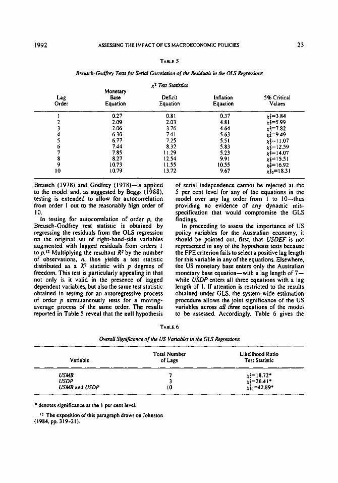
VI Specification Tests The sample period is curtailed at 1983(4) so

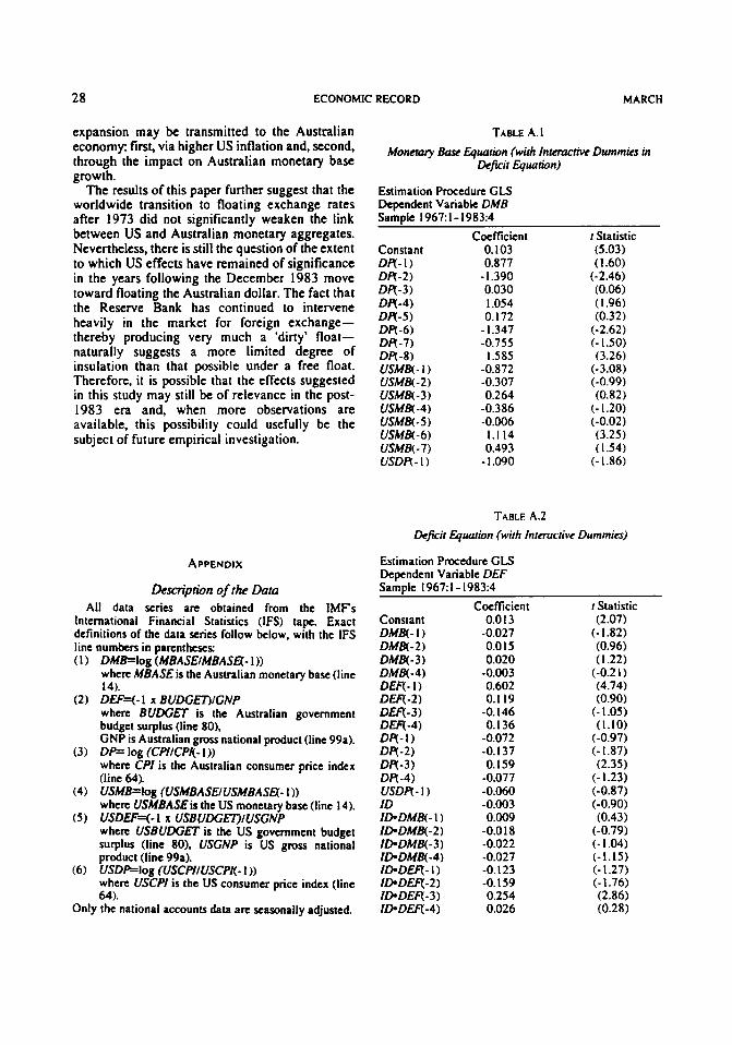
as to exclude observations that apply to the floating exchange rate regime adopted in December 1983. There remains, however, the question of a possible structural break corresponding to the introduction in September 1974 of a crawling peg by which the Australian dollar was pegged to a trade weighted basket of foreign currencies. Felmingham and Divisekera (1986, p. 33) point out that this latter regime operated more as a managed float in contrast to the earlier regime where the Australian dollar was fixed relative to. first, the pound Sterling and then the US dollar. Following Felmingham and Divisekera, the period of the managed float is assessed from 1974(4)- 1983(4) and, in order to test the stability of the model over this potential break point, a dummy variable (ID) is defined as being equal to I for the 1967( I)- 1974(3) period and zero elsewhere. This dummy is then entered additively and multiplicitively in each equation and a likelihood ratio test applied so as to test the joint significance of the full set of dummy variables. The resulting test statistic (&=79.93) is significant at the I per cent level so as to reject the null hypothesis of no structural change.

The next step concerns isolati,ng the source of the structural break. In this respect, the effects of adding the relevant set of additive and multiplicative dummies to each of the three equations is assessed with the other two equations in the system left in their original, unmodified form: that is, dummies are added to. say, the monetary base equation but not to the other two equations in the system. Here, only the deficit equation yields a test-statistic (xf4=41.60) that is significant at the 5 per cent level or better. Moreover, the difference between the value of the likelihood function when dummies are included in all three equations and the likelihood attaired when dummies are included in the deficit equation alone yields a test-statistic (xj3=38.33) that fails to be significant even at the 10 per cent level.

The results obtained when the system is re- estimated with the dummy variables included in the deficit equation are summarized in Table 8, which reports the values and significance of the sums of the lags on each variable. comparison with Table 4 reveals that the monetary base and inflation equations are little affected by the inclusion of the dummy variables, and this observation is further borne out in the detailed results for each equation under inclusion of the dummy variables (as listed in the appendix). In terms of the deficit equation itself, allowance for the dummy variables results in the responses to the domestic monetary base and to US inflation no longer being significant at the 5 per cent level under a likelihood ratio test. In particular, there is no evidence of any influence of US variables on the Australian budget deficit under the revised set of estimates.

Nevertheless, the main results concerning the impact of US monetary base growth on Australian monetary base growth and of US inflation on Australian inflation remained unaffected. Thus, despite the structural instability suggested in the deficit equation, there remains support for a significant influence of the US variables that persists through both the fixed and crawling peg exchange rate regimes. Whether the same can be said with regard to the experience after December 1983 is an issue that cannot be settled satisfactorily until more observations become available.Is

Another issue is whether the model is mis- specified in the sense that relevant variables have been omitted from the regressions. Here, Ramsey (1969) suggests a procedure (RESET) in which the estimated equations are augmented by additional test variables. If these additional test variables are jointly insignificant-in this case on the basis of a likelihood ratio test-then the null hypothesis of no specification error cannot be rejected. Kriimer er uf. (1985) suggest three sets of test variables based on (i) second and third powers of the fitted dependent variable, (ii) second powers of all right-hand-side variables included

' 3 A n attempt was made to assess the effect of adding post-I983 observations to the present sample and re- estimating. However, using multiplicative dummy variables to test for shifts in the parameters after 1983 led to singularity problems-although it may be added that, when attention was restricted to additive dummies, these proved to be insignificant in each of the three equations. (The additional years that could be included were, by necessity, limited to 1984 and 1985 due to the IMF series on the quarterly US budget deficit being curtailed at 1985(4)).

I992 ASSUSING THE IMPACT OF US MACROECONOMIC POLICIES 27

TABLE 8

GLS Results for the Sums of the Logs When Interacnve Dummies are Included in the LkficU Equation

Sum of Number of Likelihood Ratio Variable Lags Lags Test Statistic

Monetary Base DP Equation USUB

USDP

Deficit Equation

Inflation Equation

DUB DEF DP USDP ID-DMB ID-DEF D D P ID- USDP

DMB DEF DP USDP

0.226 0.300

- 1.090

0.005 0.71 I

-0. I 2 1 -0.060 -0.058 -0.002 0.246

-0. I03

0.103

0.645 0.402

-0.297

8 7 I

4 4 4 I 4 4 4 I

4 8 2 I

xi=25.5 3* xi=20.65* xi=3.37***

xi=8.57***

xi= I I .49**

xi=3.37

xj=34.23 * xizO.74

xi=22.45* xi=20.25* xi=0.47

,+2 I .87* xi=27.63* &40.53* x;=12.52*

Note: ID is a dummy variable set equal to 1 for 1967(1)- 1974(3) and 0 elsewhere.

*, ** and *** denote significance at the I per cent, 5 per cent and 10 per cent levels, respectively.

in the original regression and (iii) second and third powers of the first principal component of the regressor matrix.

Unfortunately, retrieval of the fitted values of the dependent variables is not possible under the simultaneous equation estimation procedure considered here, while addition of second powers of all the right-hand-side variables proves infeasible owing to the larg: number of explanatory variables and to the resulting singularity in the coefficient matrix. Hence, attention has to be restricted to the second and third powers of the first principal component. When these second and third powers are added to each equation in the system, however, the null hypothesis of no specification error cannot be rejected.'e In this way, neither the application of the RESET test nor the allowance for structural instability appears to call into question the main results derived in the previous section, even though the instability evidenced in the deficit equation suggests the same

When added to the specification that includes the additive and interactive dummies in the deficit equation, the relevant test statistic is given by xz=l1.92. In the case of the original specification without these dummies, the test-statistic is almost identical and is equal to 12.00,

need for caution in aggregating across fixed and crawling peg exchange rate regimes that is indicated in Felmingham and Divisekera's ( 1 986) results for the behaviour of Australia's trade balance.

Vii Conclusions This paper extends the previous literature by

examining the influence of US variables on the Australian economy in the context of a trivariate model that also allows for interactions between domestic monetary policy, fiscal policy and inflation. The results provide some support for Layton's (1983, 1986) earlier finding that lagged US monetary growth exerts a significant and positive impact on Australian monetary growth- although this effect tends to be masked by less significant and broadly negative terms appearing in the early part of the full lag distribution. At the same time, there is the additional finding that US inflation leads Australian inflation with a long- run coefficient slightly in excess of unity. In conjunction with a significant role for lagged Australian monetary base growth in the inflation equation, this draws attention to two possible channels by which higher rates of US monetary


expansion may be transmitted to the Australian economy first, via higher US inflation and, second, through the impact on Australian monetary base growth.

The results of this paper further suggest that the worldwide transition to floating exchange rates after 1973 did not significantly weaken the link between US and Australian monetary aggregates. Nevertheless, there is still the question of the extent to which US effects have remained of significance in the years following the December 1983 move toward floating the Australian dollar. The fact that the Reserve Bank has continued to intervene heavily in the market for foreign exchange- thereby producing very much a ‘dirty’ float- naturally suggests a more limited degree of insulation than that possible under a free float. Therefore, it is possible that the effects suggested in this studv mav still be of relevance in the Dost- 1983 era *and,- when more observations’ available, this possibility could usefully be subject of future empirical investigation.

APPENDIX

&scn)rion of the Data

are the

All data series are obtained from the IMF‘s International Financial Statistics (IFS) tape. Exact definitions of the data series follow below, with the IFS line numbcn in parentheses:

DMB=lOg (MBASEIMBASH- I )) where MBASEis the Australian monetary base (line 14). Dffq-1 x BUDC&T)iGNP where BUDGET is the Australian government budget surplus (line 80). GNP i s Australian gross national product (line 99a).

when CPI is the Australian consumer price index (line 64).

where USMBASEis the US monetary base (line 14).

when USBUDGET is the US government budget surplus (line 80). USGNP is US gross national product (line 99a). USDBlog (USCPIlUSCPI(- I ) ) where USCPI i s the US consumer price index (line 64).

DP= log (CPllCPI(- I ))

USMB=IO~ (USMBASUUSMBAS&- I ))

USDEFq- I x USBUDGOIUSGNP

Only the national accounts data are seasonally adjusted.

TABLE A. I hionemy Base Equation ( w i h Interactive Dummies in

Defrrit Equation)

Estimation Procedure GLS Dependent Variable DMB Sam& 1967: I - 1983:4

Constant O R - I ) DR-2) DR-3) DR-4) DPI-5) DR-6) 0 9 - 7 ) DR-8) USMBt- 1 ) USM& - 2 ) USMBt - 3) USM&-4) USM&-5 ) USU&-6) USM& - 7 ) USDR- I)

Coefficient 0. I03 0.877

0.030 I .054 0. I72

- I .390

- I .347 -0.755

1.585 -0.872 -0.307 0.264

-0.386 -0.006

1 . 1 14 0.493

- I .090

r Statistic (5.03) ( I .60)

(-2.46) (0.06) (I .96) (0.32)

(-2.62) (- I .50) (3.26)

(-3.08) (-0.99) (0.82)

(- I .20) (-0.02) (3.25) ( I .54)

(-1.86)

TABLE A.2

Deficit Equrion (wiih lniemcrive Dummies)

Estimation Procedure GLS Dependent Variable DEF Sample 1967: I - 1983:4

Coefficient 0.0 I3

-0.027 0.0 I5 0.020

-0.003 0.602 0.1 19

0. I36 -0. I46

-0.072 -0.137 0. I59

-0.077 -0.060 -0.003 0.009

-0.0 I8 -0.022 -0.027 -0. I23 -0. I59 0.254 0.026

I Statistic (2.07)

(-1.82) (0.96) (I .22)

(-0.2 I ) (4.74) (0.90)

(- I .05) (1.10)

(-0.97) (- 1.87)

(-1.23) (-0.87) (-0.90) (0.43)

(-0.79) (- I .04) ( - I . I S ) (-1.27) (- 1.76) (2.86) (0.28)

(2.35)

I992 ASSESSING THE IMPACT OF US MACROECONOMIC POLICIES 29

ID. DR - I ) -0.078 (-0.87)

ID DR- 3) -0.083 (-0.9 I )

ID USDR- I ) -0. I 03 (-0.70)

IDDR-2) 0.342 (4.8 I )

IDDR-4) 0.065 (0.83)

Note: ID is a dummy variable set equal to I for 1967( I)- 1974(3) and 0 elsewhere.

TABLE A.3

Infirion Equation (with Interactive Dummies in Defuir Equution)

Estimation Procedure GLS Dependent Variable DP Samole 1967: I - l983:4

Constant DMN- I ) D MB( - 2 ) DMN-3) DMN-4) DER- I) DER-2) DER-3) DER-4) DER-5) DER-6) DER-7) DEF( - 8) DR-I) DR-2) USDR- I )

Coefficient 0.0 I5 0.076

-0.042 0.009 0.060 0.239

0.609 -0.546

-0. I03 -0.663 0.581

-0.099 -0.3 I5 0.335 0.310 0.402

I Statistic (1.73) (3.55)

(- 1.82) (0.4 I ) (2.86) ( I .30)

(2.90) (-2.89)

(-0.48) (-3.50)

(-0.49) (- I .67)

(2.92)

(3.22) (3.14) (3.73)

REFERENCES Ahking, F.W. and Miller, S.M. (1985). 'The Relationship

Between Government Deficits. Money Growth and Inflation'. Journal of Macroeconomics 7.447-67.

Akaike. H. ( I 970). 'Statistical Predictor Identification', Ann& of the Institute of Stafkrical Mathematics 22.

Barry, P.F. (1978). 'An Indicator of Central-Bank Policy in an Open Economy', in M.G. Porter (ed.). The Ausrrahn Monetary Sysrem in rhr 1970s. Monash University. Clayton, Victoria.

Beggs, JJ. (1988). 'Diagnostic Testing in Applied Econometrics'. Economic Record 64.8 I - I0 I.

Breusch. T.S. ( I978), 'Testing for Autocornlation in Dynamic Linear Models', Ausrrahn Economic Papers

Burdekin. R.C.K ( 1989). 'International Transmission of U.S. Macroeconomic Policy and the Inflation Record of Western Europe'. J o m I of Intmatbnal M o t q and Fiance 8.40 1-23.

Camen, U.. Genberg, H. and Salemi. M. (1990), 'Optimal Monetary Policy and the Revealed Preference Function of the Swiss National Bank', in P. Artus

203- 17.

17,334-55.

and Y. Barroux (eds), Monetary Policy: A Theorerical und .&onornettic Approach. Kluwer Academic, Dordrecht. Netherlands.

Darby, M.R. (1981), 'The International Economy as a Source of and Restraint on US. Inflation'. in W.A. Gale (ed.). Infition. Causes. Consequences. and Control, Oelgeschlager. Gunn and Hain, Cambridge, Massachusetts.

-and Lothian, J.R. (1989). 'The International Transmission of Inflation Afloat', in M.D. Bordo (cd.). Money, History, and Internarionul finance: Ecrnys in Honor of Anna J. Schwam. University of Chicago Press. Chicago, Illinois.

Evans, P. (1986). 'Is the Dollar High Because of Large Budget Deficits?, lournul of Monetury Eonomics 18,

Feige, E.L. and Johannes. J.M. ( 1982). 'Was the United States Responsible for Worldwide Inflation under the Regime of Fixed Exchange Rates?'. Kyklos 35.

Felrningham. B.S. and Divisekera. S. (1986). 'The Response of Australia's Trade Balance Under Different Exchange Rate Regimes', Ausrruliuti Economic Pupen 25.33-46.

Godfrcy, L.G. (1978). 'Testing Against General Autoregressive and Moving Average Error Models when the Regressors Include Lagged Dependent Variables'. fionometricu 46, 1293- 1302.

Hopkins, S. (1988). 'Official Australian Intervention in Foreign Exchange Markets. I977 to I 986'. l2onomit.s Lwrters 26. 73-75.

Johnston, J. (1984). Econometric Methods, 3rd edn, McGraw-Hill. New York.

Krimer, W.. Sonnkrger, H.. Maurer. 1. and Havlik. P. ( 1985). 'Diagnostic Checking in Practice', Review of Economics and StatiCrics 67. I 18-23.

Laney, LO. and Willett, T.D. (1982). 'The International Liquidity Explosion and Worldwide Inflation: The Evidence from Sterilization Coefficient Estimates'. JournuloflniernarionalMontyondF~ance 1.141-52.

Layton, A.P. ( 1983). 'Is U.S. Monetary Growth a Leading Indicator of Australian Monetary Growth?. Economic

-(1986). 'A Second Look at the U.S.-Australian Monetary Growth Causal Nexus', Applied Economics

Marsden, J.S. and Jones, P.L. (1988). 'Monetary and Exchange Rate Policy: A Volatility Based Perspective', Economic Papers 7,82-93.

Masson, P. and Blundell-Wignall, A. (1985). 'Fiscal Policy and the Exchange Rate in the Big Seven: Transmission of U.S. Government Spending Shocks', Europan Economic RNicw 28, I 1-42.

Mcnick, JJ . Jr and Saundcrs. A. (1986). 'International Expected Real Interest Rates: New Tests of the Parity Hypothesis and U.S. Fiscal Policy Effects', Journal of Monetary Economics 18.3 13-22.

Opler. T.C. ( 1988). 'The Effect of Inflationary Pressure on Government Expenditure', Economics Lrtm 28, 33 1-34.

227-49.

263-77.

Record 59, 180-5.

18.443-5 I .


Parkin. M. (1977), 'A 'Monetarist' Analysis of the

Papers and

J o d of the Royal Srarirticol Sociery, Series B 31,

Rothenberg, TJ. (1984). 'Approximate Normality of Generalized Least Squam Estimates', Economcnica

Sh=han. R.G. (1987)v 'Does U.S. Money Growth Determine Money Growth in Other Nations?', Federal Reserve Bank of St Louis Review 6% 1 ), 5- 14.

Zellner, A. (1962), 'An Efficient Method of Estimating Seemingly Unrelated Regressions and Tests for Aggregation Bias', Journalof rhe American Srarirrical Associorion 57.348-68.

Generation and Transmission of Inflation: 350-7 I. 1958-1971** American Economic Proceedings 67. 164-7 1.

Flexible Exchange Rate System in the Context of External Inflation', Scandinavian Journal of Economics 87.44-65.

-and Vousden. N. (1987). 'Exchange Rates, Policy Rules and Inflation', AILmalian Economic Papers 26, 43-57.

Ramscy, J.B. (1969). 'Tats for Specification Errors in - Classical Linear Least-squares Regression Analysis',

Pitchford, J.D. (1985). 'The Insulation Capacity of a 52.8 I 1-25,

assessing the impact of us macroeconomic policies and inflation rates on the australian economy

Documents