Assessing the Impact of Trade Liberalization on Import-Competing Industries in the Appalachian Region ∗

Andrew B. Bernard Tuck School of Business at Dartmouth and NBER J. Bradford Jensen Institute for International Economics Peter K. Schott Yale School of Management and NBER July 2005

∗ This project was supported by ARC grants CO-12884S-03, CO-12884U-03, and CO-12884V-03. The research in this paper was conducted at the Center for Economic Studies. Results and conclusions are those of the authors and do not necessarily indicate concurrence by the Bureau of the Census, the NBER, or the Appalachian Regional Commission. The paper has been screened to insure that no confidential data are revealed. It has not undergone the review that Census gives its official products.

Executive Summary: Appalachian manufacturing will face significant pressure from import competition over the near and medium term and will face significantly larger adjustments than the rest of the US. The challenges faced by Appalachia are the result of a number of related factors. First, the share of manufacturing imports from low-wage countries like China and India has grown significantly over the past 30 years and especially rapidly in the last ten years. These low-wage imports are concentrated in relatively labor-intensive industries such as apparel and footwear and are relatively absent in capital-intensive, technology-intensive sectors such as transportation. Second, the arrival of low-wage imports in a sector is associated with a higher probability of manufacturing plant closure as well as lower employment and output growth. Within industries, the lowest-wage, most labor-intensive plants face the greatest threat due to imports from these low-wage countries. Third, Appalachian manufacturing employment and output are concentrated in industries facing high exposure to imports from low-wage countries. Within industries, plants in the Appalachian region are less skill-intensive and less productive than elsewhere in the US. Appalachian manufacturing is therefore more exposed to the effects of imports from low-wage countries. Fourth, in addition to being more exposed, direct measures of the impact of low-wage competition on employment growth and plant failure show a more pronounced effect of low-wage competition on Appalachian plants than on plants elsewhere in the US. Plants in the Appalachian region have higher shutdown probabilities and lower employment growth when facing low-wage imports than do firms in the rest of the US. Fifth, low-wage import shares are forecast to increase rapidly in the next decade. By 2011, low-wage countries are predicted to account for 24 percent of all US imports, up from 15 percent in 1991. More importantly, the increase will be greatest in low-wage, labor-intensive industries, precisely those sectors that are over-represented in the Appalachian region. And, while tariffs and transportation costs are not expected to undergo substantial changes in the medium term, the next decade will bring continued pressure on firms in labor-intensive industries and on firms with a labor-intensive product mix in all industries. Developments in trade policy are unlikely to dramatically alter these forecasts. Sixth, Appalachian manufacturing industries also exhibit lower levels of firm entry and exit than the US as a whole. These lower transition rates suggest that Appalachian manufacturing might be slower to adjust their product mix in response to international pressure, compounding the challenges posed by increasing import competition. The combination of these factors presents significant challenges to Appalachian manufacturing and policy-makers in the region.

i

I. Introduction:

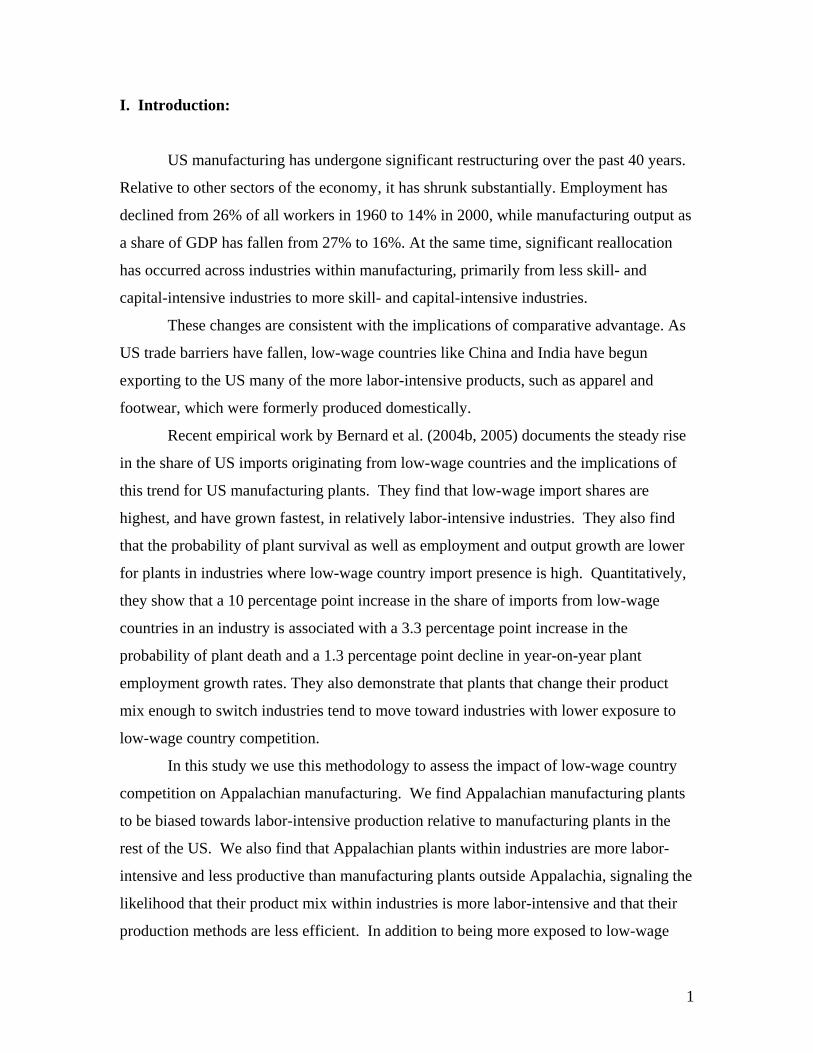
US manufacturing has undergone significant restructuring over the past 40 years.

Relative to other sectors of the economy, it has shrunk substantially. Employment has

declined from 26% of all workers in 1960 to 14% in 2000, while manufacturing output as

a share of GDP has fallen from 27% to 16%. At the same time, significant reallocation

has occurred across industries within manufacturing, primarily from less skill- and

capital-intensive industries to more skill- and capital-intensive industries.

These changes are consistent with the implications of comparative advantage. As

US trade barriers have fallen, low-wage countries like China and India have begun

exporting to the US many of the more labor-intensive products, such as apparel and

footwear, which were formerly produced domestically.

Recent empirical work by Bernard et al. (2004b, 2005) documents the steady rise

in the share of US imports originating from low-wage countries and the implications of

this trend for US manufacturing plants. They find that low-wage import shares are

highest, and have grown fastest, in relatively labor-intensive industries. They also find

that the probability of plant survival as well as employment and output growth are lower

for plants in industries where low-wage country import presence is high. Quantitatively,

they show that a 10 percentage point increase in the share of imports from low-wage

countries in an industry is associated with a 3.3 percentage point increase in the

probability of plant death and a 1.3 percentage point decline in year-on-year plant

employment growth rates. They also demonstrate that plants that change their product

mix enough to switch industries tend to move toward industries with lower exposure to

low-wage country competition.

In this study we use this methodology to assess the impact of low-wage country

competition on Appalachian manufacturing. We find Appalachian manufacturing plants

to be biased towards labor-intensive production relative to manufacturing plants in the

rest of the US. We also find that Appalachian plants within industries are more labor-

intensive and less productive than manufacturing plants outside Appalachia, signaling the

likelihood that their product mix within industries is more labor-intensive and that their

production methods are less efficient. In addition to being more exposed to low-wage

1

import competition, the response of plants in Appalachia to import competition is greater

than elsewhere in the US. For Appalachian manufacturing plants, we find that low-wage

competition has reduced the probability of plant survival and lowered employment

growth among surviving plants and this response is more pronounced than in the rest of

the US. However, at the same time, firm characteristics play a larger role in offsetting

the deleterious effects of low-wage competition in Appalachia. Skill-intensive and

capital-intensive firms are more likely to survive and grow in the Appalachian region

even in the face of increasing low-wage import exposure.

Our results are also consistent with those of Jensen (1998) in finding that wages in

Appalachia, both skilled and unskilled, are lower than they are in the rest of the United

States. These differences are driven by two biases, namely that Appalachian plants are

concentrated in labor-intensive industries and, within industries, they are more labor-

intensive than non-Appalachian plants.

The remainder of this report is structured as follows. Section II outlines the

measures we use to assess low-wage country competition. Section III compares

Appalachian manufacturing plants to those of the rest of the United States. Section IV

describes our methodology for estimating the impact of low-wage country competition on

Appalachia as well as the plant-level US manufacturing data we exploit. Section V

develops a forecast for import competition over the next decade and VI discusses

scenarios for Appalachian exposure to low-wage country import competition going

forward.

2

II. Measuring Import Competition

II.A. Share of Imports from Low-Wage Countries1

US imports of goods and services have increased rapidly over the past 20 years

from $319B in 1981 to $1,437B in 2001 (2000$), accounting for 6.0% of GDP in 1981

and 14.6% in 2001. Even as total imports have increased faster than GDP, imports

originating in low-wage countries have grown more rapidly than overall imports. As

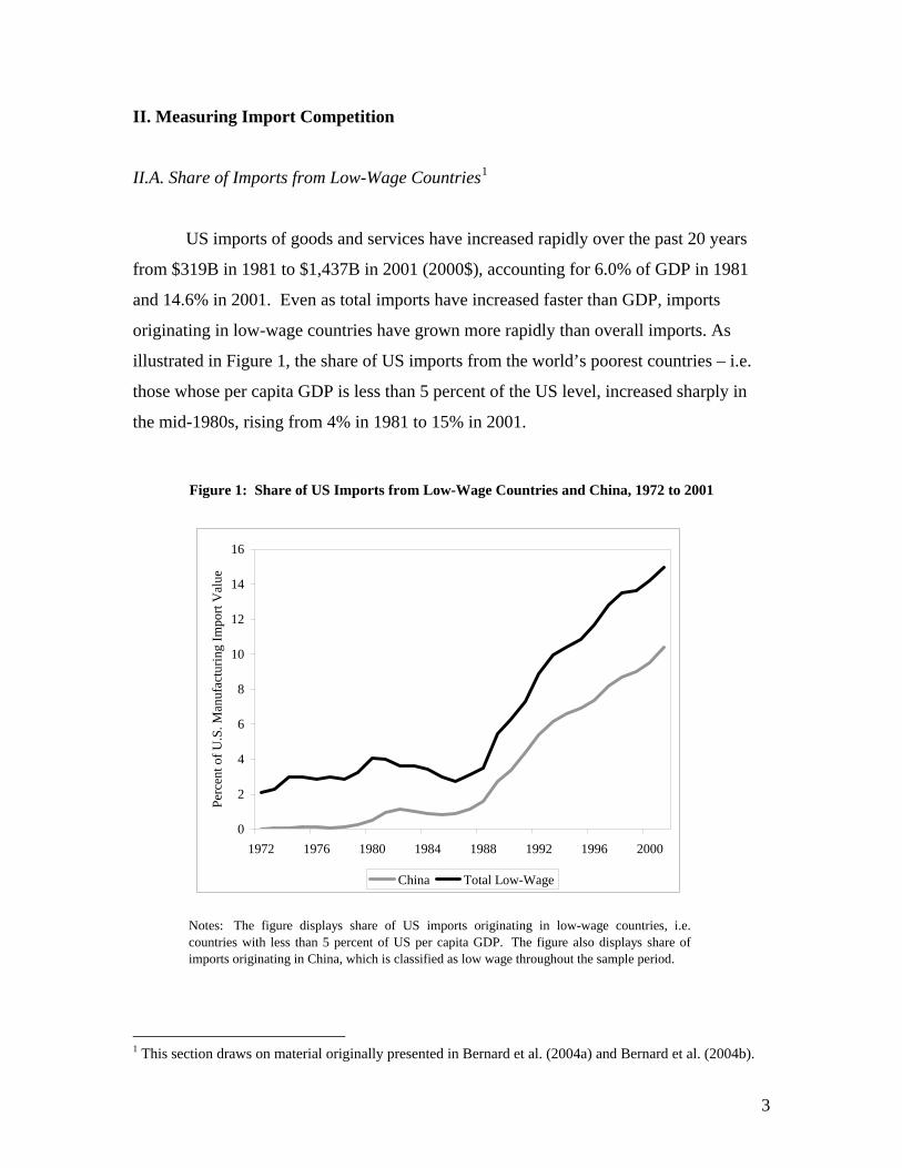
illustrated in Figure 1, the share of US imports from the world’s poorest countries – i.e.

those whose per capita GDP is less than 5 percent of the US level, increased sharply in

the mid-1980s, rising from 4% in 1981 to 15% in 2001.

Figure 1: Share of US Imports from Low-Wage Countries and China, 1972 to 2001

0

2

4

6

8

10

12

14

16

1972 1976 1980 1984 1988 1992 1996 2000

Perc

ent o

f U.S

. Man

ufac

turin

g Im

port

Val

ue

China Total Low-Wage

Notes: The figure displays share of US imports originating in low-wage countries, i.e. countries

with less than 5 percent of US per capita GDP. The figure also displays share ofimports originating in China, which is classified as low wage throughout the sample period.

1 This section draws on material originally presented in Bernard et al. (2004a) and Bernard et al. (2004b).

3

In this study we use the share of imports from low-wage countries to examine the

link between US manufacturing plant outcomes and international trade. This measure of

exposure to international competition differs from traditional measures, including import

penetration and import price indexes, by focusing on where imports originate rather than

on their level. This alternate focus is necessary because the intra- and inter-industry

reallocation implied by the factor proportions framework of international trade is a

function of trade between countries with very different relative endowments. A key

implication of the factor proportions trade model is that the goods produced in a country

are a function of its relative endowments. In an open world trading system, relatively

capital- and skill-abundant countries like the US are expected to produce a more capital-

and skill-intensive mix of industries than relatively labor-abundant countries like China.

For example the US produces pharmaceuticals and China produces t-shirts.2 For the US,

imports from China are expected to have a larger impact on manufacturing than imports

from countries like Germany whose relative capital intensity and technology intensity is

similar to those in the US. As a result, the measure of the share of imports from low-

wage countries provides a strong signal about which US industries are most exposed to

trade with low-wage countries.3

Formally, we define an industry’s exposure to imports originating in low-wage

countries in a given year as the value share of imports from low wage countries (or

VSHit), as:

VSHit = (Importsit,Low Wage / Importsit,Total)

where Importsit,Low Wage and Importsit,Total Imports are the value of imports from low-wage

countries and all countries, respectively. VSH is bounded by zero and unity, with VSH=1

indicating that all of an industry’s import value originates in low-wage countries.

2 Relative endowments of factors rather than absolute quantities drive differences in production across countries. For example, Belgium produces goods that are similar to those produced in the US while Cambodia produces products similar to those produced in China even though Belgium and Cambodia are much smaller than the US or China. 3 A number of factors, including tariff barriers, non-tariff barriers and transportation costs can induce heterogeneity of exposure, even across industries of similar labor intensity.

4

We classify a country as low-wage in year t if its per capita GDP is less than 5

percent of US per capita GDP.4 This method of classification is practical because per

capita GDP data are available for a much larger sample of countries than other measures

of relative development, e.g., manufacturing wages. Our cutoff captures an average of 50

countries per year. Table 1 lists the set of countries classified as low wage by this screen

in every year of the sample period. This set includes China and India as well as relatively

small exporters such as Haiti. Using data and concordances compiled by Feenstra (1996)

and Feenstra et al. (2002), we are able to compute VSH for 385 of 459 four-digit SIC

(SIC4) manufacturing industries. These industries encompass 88 percent of

manufacturing employment and 91 percent of manufacturing value.

We choose a 5 percent cutoff to classify countries as low wage for several

reasons. Most important, it represents the world’s most labor-abundant cohort of

countries and therefore the set of countries most likely to have an effect on US

manufacturing plants according to the factor proportions framework. Second, though this

cohort of countries is responsible for a relatively small level of exports, it accounts for a

relatively significant share of US import growth over time.5 Among countries with less

than 30 percent of US GDP per capita, the cohort of countries below the 5 percent cutoff

experienced the largest increase in import share, by far, between 1972 and 1992. Finally,

the set of countries defined by this cutoff is relatively stable in terms of countries entering

and leaving the set over the sample period we consider.6

Table 2 summarizes VSH by two-digit SIC manufacturing industry and year. The

final row of the table reports VSH for US manufacturing as a whole. Across all

4 We compare countries to the US in terms of dollar-denominated per capita GDP. We do not make purchasing power parity (PPP) adjustments to the GDP values because for countries with such low levels of income, the use of PPP-adjusted per capita GDP sharply limits the number of available countries and years due to a lack of data. 5 Even a low level of imports from low-wage countries can play a significant role in US manufacturing outcomes. The key consideration is whether or not imports from low-wage countries overlap with goods produced in the US (Leamer 1999). It is precisely the effect of such overlap that we investigate in this paper. 6 In sensitivity analyses not reported here, we obtain similar results when using cutoffs of 10 and 15 percent.

5

manufacturing, VSH increases from 2 percent in 1972 to 15 percent in 2001, with much

of this increase occurring in the most recent years.

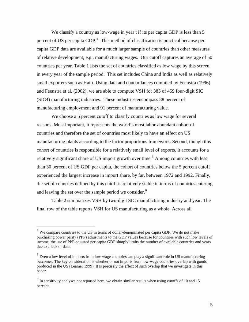
Table 1: Low-Wage US Trading Partners

Albania Ghana NigerAngola Guinea Nigeria

Bangladesh Guinea-Bissau PakistanBenin Guyana Papua New Guinea

Bolivia Haiti PhilippinesBurkina Honduras RwandaBurundi India Senegal

Cambodia Indonesia Sierra LeoneCameroon Ivory Coast Sri Lanka

Central African Republic Kenya SudanChad Laos Suriname

China (Mainland) Madagascar Syrian Arab RepublicComoros Malawi Tanzania

Congo Mali TogoCongo, Rep. Mauritania Uganda

Djibouti Mongolia VietnamEgypt Morocco Yemen Arab Republic

Equatorial Guinea Mozambique ZambiaEthiopia Nepal ZimbabweGambia Nicaragua

Notes: Countries are classified as low wage if their mean real per capita GDP isless than 5% of the U.S. level between 1972 and 2001.

The rows of Table 2 reveal that VSH varies substantially across both industries

and time. VSH is higher and increases more rapidly among generally labor-intensive

industries like Apparel, Textiles and Leather. In 2001, Transportation faced almost no

low-wage competition (1%) while the Apparel industry was heavily exposed (41%). This

contrasts sharply with the situation in 1972 when both sectors saw few imports from the

world’s poorest economies. The different experiences of these two industries reflects

their disproportionate dependence on labor: capital- and skill- intensive sectors like

Transportation are exposed to far less competition from countries like China than labor-

intensive industries like Apparel. This link between industry characteristics and low-

wage country competition adheres to the well-known theory of comparative advantage.

This theory states simply that countries specialize production according to their available

6

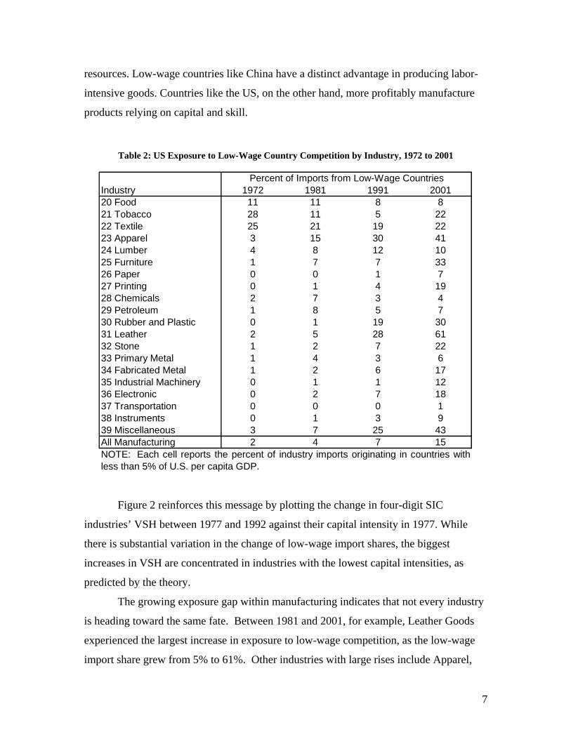
resources. Low-wage countries like China have a distinct advantage in producing labor-

intensive goods. Countries like the US, on the other hand, more profitably manufacture

products relying on capital and skill.

Table 2: US Exposure to Low-Wage Country Competition by Industry, 1972 to 2001

Industry 1972 1981 1991 200120 Food 11 11 8 821 Tobacco 28 11 5 2222 Textile 25 21 19 2223 Apparel 3 15 30 4124 Lumber 4 8 12 1025 Furniture 1 7 7 3326 Paper 0 0 1 727 Printing 0 1 4 1928 Chemicals 2 7 3 429 Petroleum 1 8 5 730 Rubber and Plastic 0 1 19 3031 Leather 2 5 28 6132 Stone 1 2 7 2233 Primary Metal 1 4 3 634 Fabricated Metal 1 2 6 1735 Industrial Machinery 0 1 1 1236 Electronic 0 2 7 1837 Transportation 0 0 0 138 Instruments 0 1 3 939 Miscellaneous 3 7 25 43All Manufacturing 2 4 7 15

Percent of Imports from Low-Wage Countries

NOTE: Each cell reports the percent of industry imports originating in countries withless than 5% of U.S. per capita GDP.

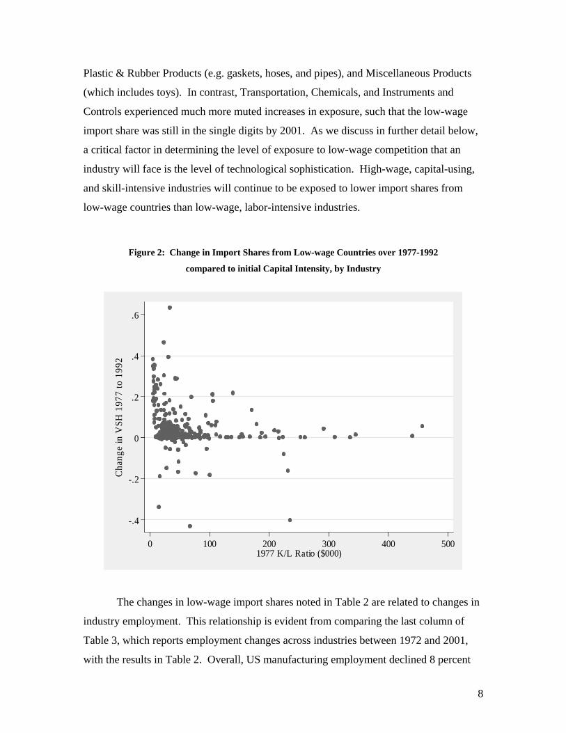
Figure 2 reinforces this message by plotting the change in four-digit SIC

industries’ VSH between 1977 and 1992 against their capital intensity in 1977. While

there is substantial variation in the change of low-wage import shares, the biggest

increases in VSH are concentrated in industries with the lowest capital intensities, as

predicted by the theory.

The growing exposure gap within manufacturing indicates that not every industry

is heading toward the same fate. Between 1981 and 2001, for example, Leather Goods

experienced the largest increase in exposure to low-wage competition, as the low-wage

import share grew from 5% to 61%. Other industries with large rises include Apparel,

7

Plastic & Rubber Products (e.g. gaskets, hoses, and pipes), and Miscellaneous Products

(which includes toys). In contrast, Transportation, Chemicals, and Instruments and

Controls experienced much more muted increases in exposure, such that the low-wage

import share was still in the single digits by 2001. As we discuss in further detail below,

a critical factor in determining the level of exposure to low-wage competition that an

industry will face is the level of technological sophistication. High-wage, capital-using,

and skill-intensive industries will continue to be exposed to lower import shares from

low-wage countries than low-wage, labor-intensive industries.

Figure 2: Change in Import Shares from Low-wage Countries over 1977-1992

compared to initial Capital Intensity, by Industry

-.4

-.2

0

.2

.4

.6

Cha

nge

in V

SH 1

977

to 1

992

0 100 200 300 400 5001977 K/L Ratio ($000)

The changes in low-wage import shares noted in Table 2 are related to changes in

industry employment. This relationship is evident from comparing the last column of

Table 3, which reports employment changes across industries between 1972 and 2001,

with the results in Table 2. Overall, US manufacturing employment declined 8 percent

8

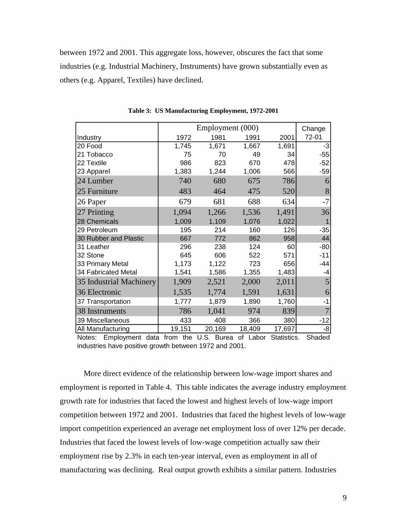
between 1972 and 2001. This aggregate loss, however, obscures the fact that some

industries (e.g. Industrial Machinery, Instruments) have grown substantially even as

others (e.g. Apparel, Textiles) have declined.

Table 3: US Manufacturing Employment, 1972-2001

Industry 1972 1981 1991 200120 Food 1,745 1,671 1,667 1,691 -321 Tobacco 75 70 49 34 -5522 Textile 986 823 670 478 -5223 Apparel 1,383 1,244 1,006 566 -5924 Lumber 740 680 675 786 625 Furniture 483 464 475 520 826 Paper 679 681 688 634 -727 Printing 1,094 1,266 1,536 1,491 3628 Chemicals 1,009 1,109 1,076 1,022 129 Petroleum 195 214 160 126 -3530 Rubber and Plastic 667 772 862 958 4431 Leather 296 238 124 60 -8032 Stone 645 606 522 571 -1133 Primary Metal 1,173 1,122 723 656 -4434 Fabricated Metal 1,541 1,586 1,355 1,483 -435 Industrial Machinery 1,909 2,521 2,000 2,011 536 Electronic 1,535 1,774 1,591 1,631 637 Transportation 1,777 1,879 1,890 1,760 -138 Instruments 786 1,041 974 839 739 Miscellaneous 433 408 366 380 -12All Manufacturing 19,151 20,169 18,409 17,697 -8Notes: Employment data from the U.S. Burea of Labor Statistics. Shadedindustries have positive growth between 1972 and 2001.

Percent Change 72-01

Employment (000)

More direct evidence of the relationship between low-wage import shares and

employment is reported in Table 4. This table indicates the average industry employment

growth rate for industries that faced the lowest and highest levels of low-wage import

competition between 1972 and 2001. Industries that faced the highest levels of low-wage

import competition experienced an average net employment loss of over 12% per decade.

Industries that faced the lowest levels of low-wage competition actually saw their

employment rise by 2.3% in each ten-year interval, even as employment in all of

manufacturing was declining. Real output growth exhibits a similar pattern. Industries

9

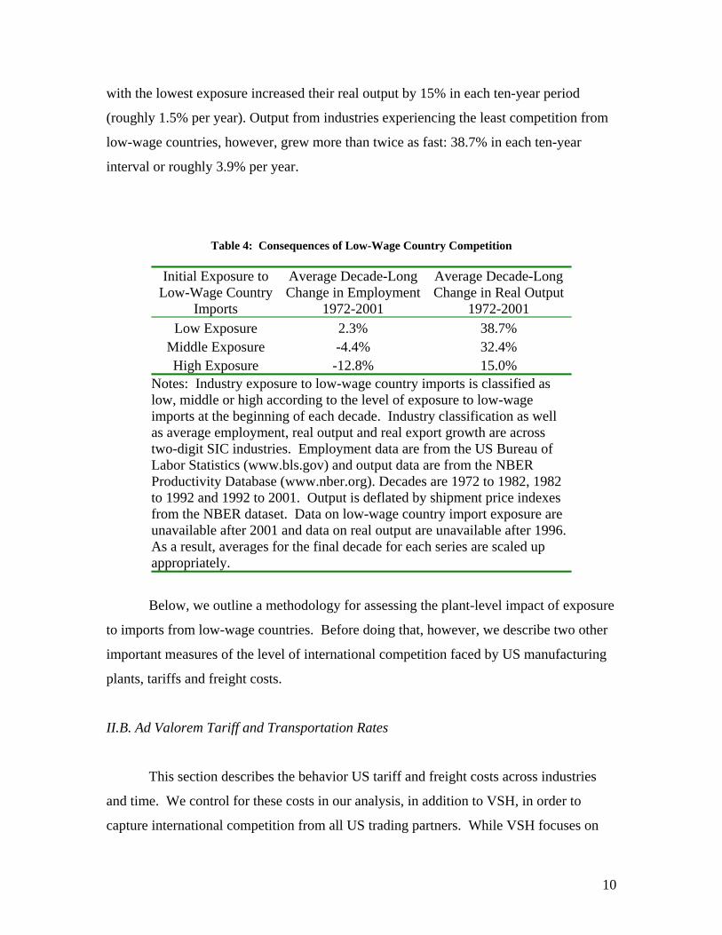
with the lowest exposure increased their real output by 15% in each ten-year period

(roughly 1.5% per year). Output from industries experiencing the least competition from

low-wage countries, however, grew more than twice as fast: 38.7% in each ten-year

interval or roughly 3.9% per year.

Table 4: Consequences of Low-Wage Country Competition

Initial Exposure to Low-Wage Country

Imports

Average Decade-Long Change in Employment

1972-2001

Average Decade-Long Change in Real Output

1972-2001 Low Exposure 2.3% 38.7%

Middle Exposure -4.4% 32.4% High Exposure -12.8% 15.0%

Notes: Industry exposure to low-wage country imports is classified as low, middle or high according to the level of exposure to low-wage imports at the beginning of each decade. Industry classification as well as average employment, real output and real export growth are across two-digit SIC industries. Employment data are from the US Bureau of Labor Statistics (www.bls.gov) and output data are from the NBER Productivity Database (www.nber.org). Decades are 1972 to 1982, 1982 to 1992 and 1992 to 2001. Output is deflated by shipment price indexes from the NBER dataset. Data on low-wage country import exposure are unavailable after 2001 and data on real output are unavailable after 1996. As a result, averages for the final decade for each series are scaled up appropriately.

Below, we outline a methodology for assessing the plant-level impact of exposure

to imports from low-wage countries. Before doing that, however, we describe two other

important measures of the level of international competition faced by US manufacturing

plants, tariffs and freight costs.

II.B. Ad Valorem Tariff and Transportation Rates

This section describes the behavior US tariff and freight costs across industries

and time. We control for these costs in our analysis, in addition to VSH, in order to

capture international competition from all US trading partners. While VSH focuses on

10

competition with countries like China, tariff and freight costs measure competitive effects

from all trading partners, whether or not their wages are low.

We use estimates of industry-year ad valorem tariff (tit) and freight and insurance

(fit) rates assembled in Bernard et al. (2003). These estimates are computed from

product-level US import data complied by Feenstra et al (2003). The tariff or freight rate

for industry i is the weighted average rate across all products in i, using the import values

from all source countries as weights. The ad valorem tariff rate is therefore duties

collected (dutiesit) relative to the Free-On-Board customs value of imports (fobit),

fit = dutiesit / fobit

Similarly, the ad valorem freight rate is the markup of the Customs-Insurance-Freight

value (cifit) over fobit relative to fobit,

fit = cifit / fobit - 1

Estimated tariff and freight rates by two-digit SIC industry and year are displayed

in Table 5. 7 Tariff rates vary substantially across industries and generally decline with

time. They are higher in labor-intensive industries like Apparel and lower in capital-

intensive sectors like Paper. Over the entire period, tariffs decline by more than one

quarter in thirteen of twenty industries. The pace of these declines, however, varies

substantially across industries.

Freight costs are highest among industries producing goods with a low value-to-

weight ratio, including Stone, Lumber, Furniture, and Food. Freight costs also generally

decline with time, though the pattern of declines is decidedly more mixed than it is with

tariffs.

7 Data on the tariff and freight measures for all 337 (SIC4) industries and years is available at http://www.som.yale.edu/faculty/pks4/sub_international.htm.

11

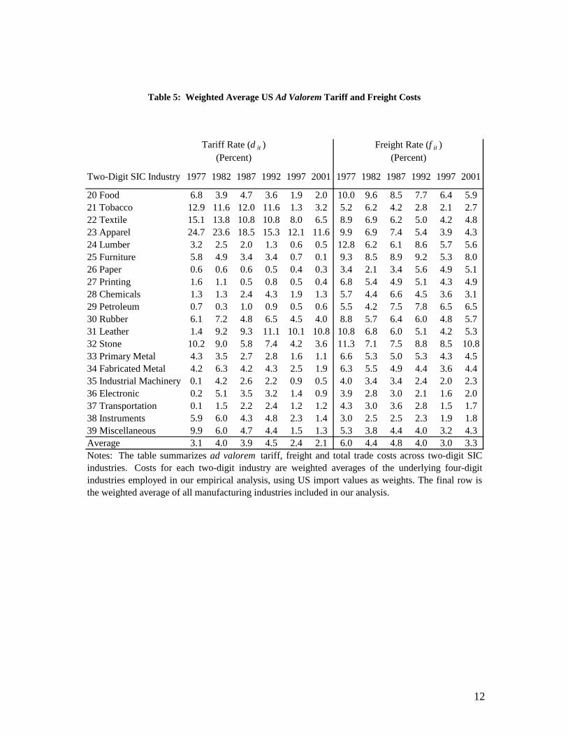
Table 5: Weighted Average US Ad Valorem Tariff and Freight Costs

Two-Digit SIC Industry 1977 1982 1987 1992 1997 2001 1977 1982 1987 1992 1997 2001

20 Food 6.8 3.9 4.7 3.6 1.9 2.0 10.0 9.6 8.5 7.7 6.4 5.921 Tobacco 12.9 11.6 12.0 11.6 1.3 3.2 5.2 6.2 4.2 2.8 2.1 2.722 Textile 15.1 13.8 10.8 10.8 8.0 6.5 8.9 6.9 6.2 5.0 4.2 4.823 Apparel 24.7 23.6 18.5 15.3 12.1 11.6 9.9 6.9 7.4 5.4 3.9 4.324 Lumber 3.2 2.5 2.0 1.3 0.6 0.5 12.8 6.2 6.1 8.6 5.7 5.625 Furniture 5.8 4.9 3.4 3.4 0.7 0.1 9.3 8.5 8.9 9.2 5.3 8.026 Paper 0.6 0.6 0.6 0.5 0.4 0.3 3.4 2.1 3.4 5.6 4.9 5.127 Printing 1.6 1.1 0.5 0.8 0.5 0.4 6.8 5.4 4.9 5.1 4.3 4.928 Chemicals 1.3 1.3 2.4 4.3 1.9 1.3 5.7 4.4 6.6 4.5 3.6 3.129 Petroleum 0.7 0.3 1.0 0.9 0.5 0.6 5.5 4.2 7.5 7.8 6.5 6.530 Rubber 6.1 7.2 4.8 6.5 4.5 4.0 8.8 5.7 6.4 6.0 4.8 5.731 Leather 1.4 9.2 9.3 11.1 10.1 10.8 10.8 6.8 6.0 5.1 4.2 5.332 Stone 10.2 9.0 5.8 7.4 4.2 3.6 11.3 7.1 7.5 8.8 8.5 10.833 Primary Metal 4.3 3.5 2.7 2.8 1.6 1.1 6.6 5.3 5.0 5.3 4.3 4.534 Fabricated Metal 4.2 6.3 4.2 4.3 2.5 1.9 6.3 5.5 4.9 4.4 3.6 4.435 Industrial Machinery 0.1 4.2 2.6 2.2 0.9 0.5 4.0 3.4 3.4 2.4 2.0 2.336 Electronic 0.2 5.1 3.5 3.2 1.4 0.9 3.9 2.8 3.0 2.1 1.6 2.037 Transportation 0.1 1.5 2.2 2.4 1.2 1.2 4.3 3.0 3.6 2.8 1.5 1.738 Instruments 5.9 6.0 4.3 4.8 2.3 1.4 3.0 2.5 2.5 2.3 1.9 1.839 Miscellaneous 9.9 6.0 4.7 4.4 1.5 1.3 5.3 3.8 4.4 4.0 3.2 4.3Average 3.1 4.0 3.9 4.5 2.4 2.1 6.0 4.4 4.8 4.0 3.0 3.3Notes: The table summarizes ad valorem tariff, freight and total trade costs across two-digit SICindustries. Costs for each two-digit industry are weighted averages of the underlying four-digitindustries employed in our empirical analysis, using US import values as weights. The final row isthe weighted average of all manufacturing industries included in our analysis.

Tariff Rate (d it ) Freight Rate (f it )(Percent) (Percent)

12

III. Differences Between Appalachian and Rest-of-US Manufacturing Plants

In this section we compare Appalachian manufacturing plants to manufacturing

plants in the rest of the United States along four key dimensions:

• The distribution of employment across industries

• The distribution of output across industries

• Plant entry and exit rates

• Exposure to international competition

We find Appalachian plants to be more heavily concentrated in labor-intensive industries,

and to be more labor-intensive within industries, than manufacturing plants in the rest of

the United States. We also find less plant entry and exit across industries in Appalachia.

A result of these trends is that Appalachia is relatively more exposed to competition from

low-wage countries.

III.A. Distribution of Employment and Output

Though the distribution of Appalachian employment and output has become more

similar to the rest of the United States over time, it is still biased toward labor-intensive

industries and labor-intensive, lower-wage and less productive plants within those

industries. Figure 3 and Figure 4 compare the aggregate output and employment of

Appalachian manufacturing plants with those of the Rest of the US (ROUS). (These

figures are based on the data displayed in Table 6 and Table 7.) Each bar in the figure

displays the difference between the share of that industry in Appalachia versus its share

in ROUS. The first bars of Figure 3, for example, indicate that Appalachia is more

heavily weighted toward Primary Metal production than ROUS, but that this difference

has decreased with time. The fact that most bars are shorter in 1997 than in 1992

indicates that Appalachia has converged toward the rest of the country over time.

13

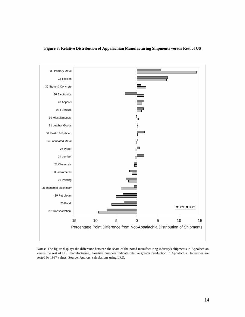
Figure 3: Relative Distribution of Appalachian Manufacturing Shipments versus Rest of US

Notes: The figure displays the difference between the share of the noted manufacturing industry's shipments in Appalachianversus the rest of U.S. manufacturing. Positive numbers indicate relative greater production in Appalachia. Industries aresorted by 1997 values. Source: Authors' calculations using LRD.

-15 -10 -5 0 5 10 15

37 Transportation

20 Food

29 Petroleum

35 Industrial Machinery

27 Printing

38 Instruments

28 Chemicals

24 Lumber

26 Paper

34 Fabricated Metal

30 Plastic & Rubber

31 Leather Goods

39 Miscellaneous

25 Furniture

23 Apparel

36 Electronics

32 Stone & Concrete

22 Textiles

33 Primary Metal

Percentage Point Difference from Not-Appalachia Distribution of Shipments

1972 1997

14

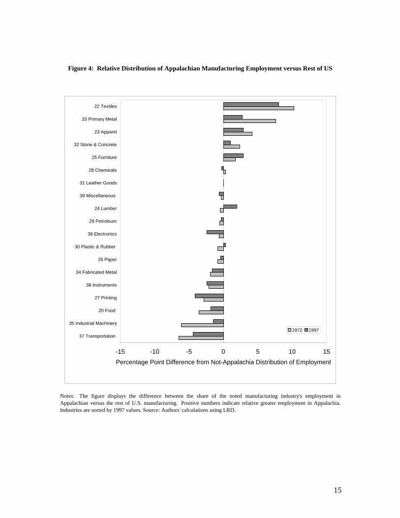
Figure 4: Relative Distribution of Appalachian Manufacturing Employment versus Rest of US

Notes: The figure displays the difference between the share of the noted manufacturing industry's employment inAppalachian versus the rest of U.S. manufacturing. Positive numbers indicate relative greater employment in Appalachia.Industries are sorted by 1997 values. Source: Authors' calculations using LRD.

-15 -10 -5 0 5 10 15

37 Transportation

35 Industrial Machinery

20 Food

27 Printing

38 Instruments

34 Fabricated Metal

26 Paper

30 Plastic & Rubber

36 Electronics

29 Petroleum

24 Lumber

39 Miscellaneous

31 Leather Goods

28 Chemicals

25 Furniture

32 Stone & Concrete

23 Apparel

33 Primary Metal

22 Textiles

Percentage Point Difference from Not-Appalachia Distribution of Employment

1972 1997

15

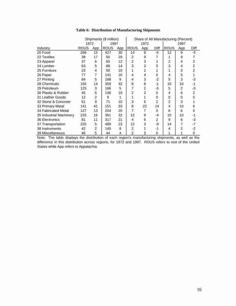
Table 6: Distribution of Manufacturing Shipments

ROUS App Diff20 Food 266 15 427 30 14 8 -6 12 9 -322 Textiles 38 17 50 29 2 9 7 1 9 723 Apparel 37 6 65 12 2 3 1 2 4 224 Lumber 63 5 88 14 3 3 0 3 4 225 Furniture 23 4 50 10 1 2 1 1 3 226 Paper 77 7 141 16 4 4 0 4 5 127 Printing 84 5 188 9 4 3 -2 5 3 -328 Chemicals 155 14 359 32 8 8 -1 10 10 -129 Petroleum 125 3 166 5 7 2 -5 5 2 -330 Plastic & Rubber 45 5 136 19 2 3 0 4 6 231 Leather Goods 12 2 9 1 1 1 0 0 0 032 Stone & Concrete 51 9 71 10 3 5 2 2 3 133 Primary Metal 141 41 151 33 8 22 14 4 10 634 Fabricated Metal 127 13 204 20 7 7 0 6 6 035 Industrial Machinery 233 16 361 32 12 9 -4 10 10 -136 Electronics 81 11 317 21 4 6 2 9 6 -337 Transportation 225 5 489 23 12 3 -9 14 7 -738 Instruments 42 2 145 8 2 1 -1 4 2 -239 Miscellaneous 46 5 44 4 2 3 0 1 1 0

1972 1997Share of All Manufacturing (Percent)Shipments ($ million)

1972 1997

Note: The table displays the distribution of each region's manufacturing shipments, as well as thedifference in this distribution across regions, for 1972 and 1997. ROUS refers to rest of the UnitedStates while App refers to Appalachia.

Industry ROUS App ROUS App ROUS App Diff

16

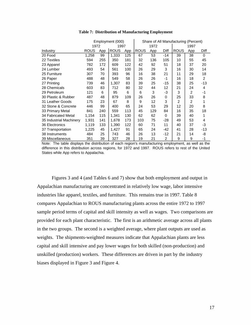
Table 7: Distribution of Manufacturing Employment

Industry ROUS App ROUS App ROUS App Diff ROUS App Diff20 Food 1,258 99 1,333 125 67 53 -14 39 38 022 Textiles 594 255 350 181 32 136 105 10 55 4523 Apparel 782 172 609 122 42 92 51 18 37 2024 Lumber 493 54 561 100 26 29 3 16 30 1425 Furniture 307 70 393 96 16 38 21 11 29 1826 Paper 488 48 549 58 26 26 -1 16 18 227 Printing 739 46 1,307 83 39 25 -15 38 25 -1328 Chemicals 603 83 712 80 32 44 12 21 24 429 Petroleum 121 6 95 6 6 3 -3 3 2 -130 Plastic & Rubber 487 48 879 109 26 26 0 25 33 831 Leather Goods 175 23 67 8 9 12 3 2 2 132 Stone & Concrete 446 99 400 65 24 53 29 12 20 833 Primary Metal 841 240 559 113 45 129 84 16 35 1834 Fabricated Metal 1,154 115 1,341 130 62 62 0 39 40 135 Industrial Machinery 1,931 141 1,678 173 103 75 -28 49 53 436 Electronics 1,119 133 1,390 122 60 71 11 40 37 -337 Transportation 1,225 45 1,427 91 65 24 -42 41 28 -1338 Instruments 484 25 743 46 26 13 -12 21 14 -839 Miscellaneous 351 39 327 28 19 21 2 9 9 -1

1972 1997

Note: The table displays the distribution of each region's manufacturing employment, as well as thedifference in this distribution across regions, for 1972 and 1997. ROUS refers to rest of the UnitedStates while App refers to Appalachia.

1972 1997Employment (000) Share of All Manufacturing (Percent)

Figures 3 and 4 (and Tables 6 and 7) show that both employment and output in

Appalachian manufacturing are concentrated in relatively low wage, labor intensive

industries like apparel, textiles, and furniture. This remains true in 1997. Table 8

compares Appalachian to ROUS manufacturing plants across the entire 1972 to 1997

sample period terms of capital and skill intensity as well as wages. Two comparisons are

provided for each plant characteristic. The first is an arithmetic average across all plants

in the two groups. The second is a weighted average, where plant outputs are used as

weights. The shipments-weighted measures indicate that Appalachian plants are less

capital and skill intensive and pay lower wages for both skilled (non-production) and

unskilled (production) workers. These differences are driven in part by the industry

biases displayed in Figure 3 and Figure 4.

17

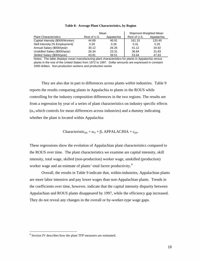
Table 8: Average Plant Characteristics, by Region

Plant Characteristics Rest of U.S. Appalachia Rest of U.S. AppalachiaCapital Intensity ($000/Worker) 44.69 46.91 161.15 120.40Skill Intensity (% Employment) 0.29 0.26 0.31 0.25Annual Salary ($000/year) 30.12 26.26 41.12 34.92Unskilled Salary ($000/year) 26.34 23.31 36.84 31.83Skilled Salary ($000/year) 43.81 39.51 53.64 47.63

Mean Shipment-Weighted Mean

Notes: The table displays mean manufacturing plant characteristics for plants in Appalachia versus plants in the rest of the United States from 1972 to 1997. Dollar amounts are expressed in constant 2000 dollars. Non-production workers and production worke

They are also due in part to differences across plants within industries. Table 9

reports the results comparing plants in Appalachia to plants in the ROUS while

controlling for the industry composition differences in the two regions. The results are

from a regression by year of a series of plant characteristics on industry specific effects

(αit which controls for mean differences across industries) and a dummy indicating

whether the plant is located within Appalachia:

Characteristicpit = αit + βt APPALACHIA + εpit.

These regressions show the evolution of Appalachian plant characteristics compared to

the ROUS over time. The plant characteristics we examine are capital intensity, skill

intensity, total wage, skilled (non-production) worker wage, unskilled (production)

worker wage and an estimate of plants’ total factor productivity.8

Overall, the results in Table 9 indicate that, within-industries, Appalachian plants

are more labor intensive and pay lower wages than non-Appalachian plants. Trends in

the coefficients over time, however, indicate that the capital intensity disparity between

Appalachian and ROUS plants disappeared by 1997, while the efficiency gap increased.

They do not reveal any changes in the overall or by-worker-type wage gaps.

8 Section IV describes how the plant TFP measures are estimated.

18

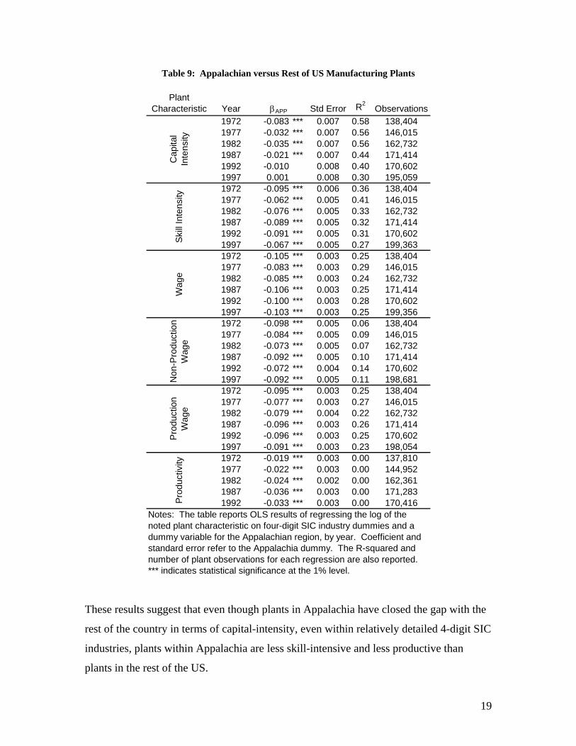
Table 9: Appalachian versus Rest of US Manufacturing Plants

Plant Characteristic Year Std Error R2

Observations1972 -0.083 *** 0.007 0.58 138,4041977 -0.032 *** 0.007 0.56 146,0151982 -0.035 *** 0.007 0.56 162,7321987 -0.021 *** 0.007 0.44 171,4141992 -0.010 0.008 0.40 170,6021997 0.001 0.008 0.30 195,0591972 -0.095 *** 0.006 0.36 138,4041977 -0.062 *** 0.005 0.41 146,0151982 -0.076 *** 0.005 0.33 162,7321987 -0.089 *** 0.005 0.32 171,4141992 -0.091 *** 0.005 0.31 170,6021997 -0.067 *** 0.005 0.27 199,3631972 -0.105 *** 0.003 0.25 138,4041977 -0.083 *** 0.003 0.29 146,0151982 -0.085 *** 0.003 0.24 162,7321987 -0.106 *** 0.003 0.25 171,4141992 -0.100 *** 0.003 0.28 170,6021997 -0.103 *** 0.003 0.25 199,3561972 -0.098 *** 0.005 0.06 138,4041977 -0.084 *** 0.005 0.09 146,0151982 -0.073 *** 0.005 0.07 162,7321987 -0.092 *** 0.005 0.10 171,4141992 -0.072 *** 0.004 0.14 170,6021997 -0.092 *** 0.005 0.11 198,6811972 -0.095 *** 0.003 0.25 138,4041977 -0.077 *** 0.003 0.27 146,0151982 -0.079 *** 0.004 0.22 162,7321987 -0.096 *** 0.003 0.26 171,4141992 -0.096 *** 0.003 0.25 170,6021997 -0.091 *** 0.003 0.23 198,0541972 -0.019 *** 0.003 0.00 137,8101977 -0.022 *** 0.003 0.00 144,9521982 -0.024 *** 0.002 0.00 162,3611987 -0.036 *** 0.003 0.00 171,2831992 -0.033 *** 0.003 0.00 170,416

Pro

duct

ion

Wag

eW

age

βAPP

Notes: The table reports OLS results of regressing the log of the noted plant characteristic on four-digit SIC industry dummies and a dummy variable for the Appalachian region, by year. Coefficient and standard error refer to the Appalachia dummy. The R-squared and number of plant observations for each regression are also reported. *** indicates statistical significance at the 1% level.

Prod

uctiv

ityC

apita

l In

tens

itySk

ill In

tens

ityN

on-P

rodu

ctio

n W

age

These results suggest that even though plants in Appalachia have closed the gap with the

rest of the country in terms of capital-intensity, even within relatively detailed 4-digit SIC

industries, plants within Appalachia are less skill-intensive and less productive than

plants in the rest of the US.

19

III.B. Industry Entry and Exit

Consistent with research reported in Jensen (1998) and Foster (2004), we find

Appalachian manufacturing to be less dynamic than manufacturing in the rest of the

United States. Table 10 documents that Appalachian manufacturing industries

experience both lower entry and exit rates than the US as a whole. Appalachian entry

rates are lower in 10 of the 19 two-digit SIC industries while exit rates are lower in 17.

For example, exit rates in Apparel and Furniture are 8 percentage points and 6 percentage

points lower, respectively, in Appalachia than in the ROUS.

These differences in entry and exit rates take on a particular importance in the

context of international competition. Lower entry and exit rates signal increased barriers

to firm formation and industries that are less able to respond to external shocks. As low-

wage countries enter US markets, one path for firms to avoid decline and shutdown is to

change product mix and enter new markets. Bernard, Redding and Schott (2004) show

that product market entry is higher in dynamic industries, i.e. industries with greater entry

and exit rates. Lower firm entry and exit rates in the Appalachian region may inhibit

firms’ abilities to get out of the way of international competition.

20

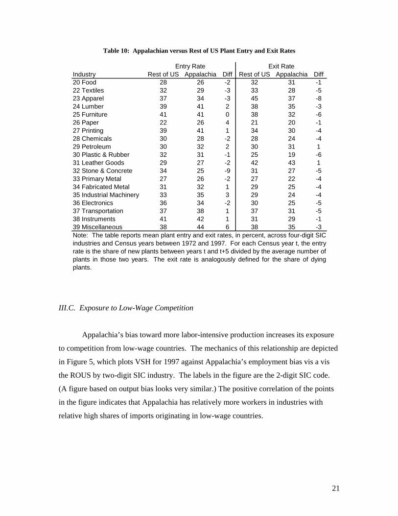
Table 10: Appalachian versus Rest of US Plant Entry and Exit Rates

Industry Rest of US Appalachia Diff Rest of US Appalachia Diff20 Food 28 26 -2 32 31 -122 Textiles 32 29 -3 33 28 -523 Apparel 37 34 -3 45 37 -824 Lumber 39 41 2 38 35 -325 Furniture 41 41 0 38 32 -626 Paper 22 26 4 21 20 -127 Printing 39 41 1 34 30 -428 Chemicals 30 28 -2 28 24 -429 Petroleum 30 32 2 30 31 130 Plastic & Rubber 32 31 -1 25 19 -631 Leather Goods 29 27 -2 42 43 132 Stone & Concrete 34 25 -9 31 27 -533 Primary Metal 27 26 -2 27 22 -434 Fabricated Metal 31 32 1 29 25 -435 Industrial Machinery 33 35 3 29 24 -436 Electronics 36 34 -2 30 25 -537 Transportation 37 38 1 37 31 -538 Instruments 41 42 1 31 29 -139 Miscellaneous 38 44 6 38 35 -3

Exit Rate

Note: The table reports mean plant entry and exit rates, in percent, across four-digit SICindustries and Census years between 1972 and 1997. For each Census year t, the entryrate is the share of new plants between years t and t+5 divided by the average number ofplants in those two years. The exit rate is analogously defined for the share of dyingplants.

Entry Rate

III.C. Exposure to Low-Wage Competition

Appalachia’s bias toward more labor-intensive production increases its exposure

to competition from low-wage countries. The mechanics of this relationship are depicted

in Figure 5, which plots VSH for 1997 against Appalachia’s employment bias vis a vis

the ROUS by two-digit SIC industry. The labels in the figure are the 2-digit SIC code.

(A figure based on output bias looks very similar.) The positive correlation of the points

in the figure indicates that Appalachia has relatively more workers in industries with

relative high shares of imports originating in low-wage countries.

21

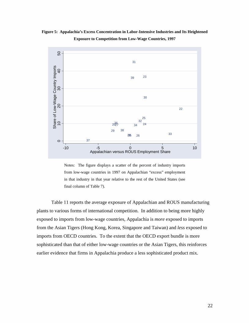
Figure 5: Appalachia’s Excess Concentration in Labor-Intensive Industries and Its Heightened

Exposure to Competition from Low-Wage Countries, 1997

20

22

23

24

25

26

27

2829

30

31

32

33

34

35

36

37

38

39

010

2030

4050

Sha

re o

f Low

-Wag

e C

ount

ry Im

ports

-10 -5 0 5 10Appalachian versus ROUS Employment Share

Notes: The figure displays a scatter of the percent of industry imports

from low-wage countries in 1997 on Appalachian “excess” employment

in that industry in that year relative to the rest of the United States (see

final column of Table 7).

Table 11 reports the average exposure of Appalachian and ROUS manufacturing

plants to various forms of international competition. In addition to being more highly

exposed to imports from low-wage countries, Appalachia is more exposed to imports

from the Asian Tigers (Hong Kong, Korea, Singapore and Taiwan) and less exposed to

imports from OECD countries. To the extent that the OECD export bundle is more

sophisticated than that of either low-wage countries or the Asian Tigers, this reinforces

earlier evidence that firms in Appalachia produce a less sophisticated product mix.

22

Table 11: Average Trade Exposure Across Plants, by Region

Country Group Rest of U.S. Appalachia Rest of U.S. AppalachiaLow-Wage Countries 5.02 6.02 4.01 6.42Tiger Countries 6.07 6.35 4.07 4.67OECD Countries 71.87 69.63 72.91 70.93Ad Valorem Tariff Rate 4.08 4.79 3.20 4.95Ad Valorem Freight Rate 5.62 5.97 5.15 5.54

Mean Shipment-Weighted Mean

Notes: The first three rows of the table display mean share of imports from noted countries acrossplants based on their four-digit SIC industry classification. Low-wage countries are defined as countrieswith less than 5% of U.S. per capita GDP. Tiger countries are Hong Kong, Korea, Singapore andTaiwan. OECD countries are the 22 members as of 1972 (i.e. excluding recent entrants such as Koreaand Mexico). The final two rows in each section report average ad valorem tariff and transport costs.The left panel reports arithmatic means while the right panel reports shipment-weighted means.

The final two rows of Table 11 report the average import tariffs and transport

costs weighted by industrial output for Appalachia and ROUS. The industrial mix in the

Appalachian region is composed of relatively high-tariff, high transport cost sectors. On

an output-weighted basis, tariffs on goods in Appalachia are 1.8 percentage points, or 54

percent, higher than for the rest of the US. These higher levels of protection and

transport costs have somewhat insulated industries in the Appalachian region from the

pressure of import competition.

However, these pooled numbers hide a faster decline in tariffs for Appalachian

industries over time as can be seen in Table 12. In 1977, output-weighted tariff levels

were 6.3 percent in Appalachia and 3.6 percent in the ROUS. By 1997, tariffs levels had

fallen to 2.4 percent and 1.7 percent in the two regions respectively. Similarly the gap in

transport costs narrows over time between the Appalachian region and the ROUS. The

more rapid decline in tariffs and transport costs for industries in Appalachia suggests that

these traditional barriers to import competition are declining.

23

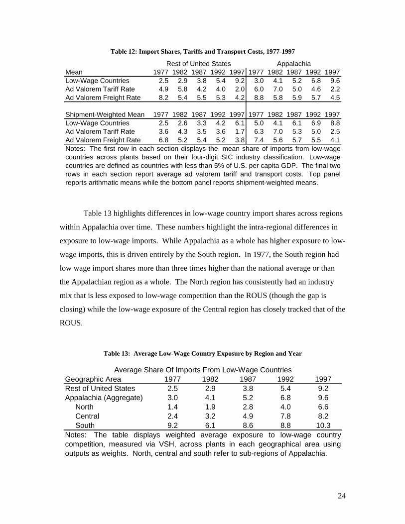
Table 12: Import Shares, Tariffs and Transport Costs, 1977-1997

Mean 1977 1982 1987 1992 1997 1977 1982 1987 1992 1997Low-Wage Countries 2.5 2.9 3.8 5.4 9.2 3.0 4.1 5.2 6.8 9.6Ad Valorem Tariff Rate 4.9 5.8 4.2 4.0 2.0 6.0 7.0 5.0 4.6 2.2Ad Valorem Freight Rate 8.2 5.4 5.5 5.3 4.2 8.8 5.8 5.9 5.7 4.5

Shipment-Weighted Mean 1977 1982 1987 1992 1997 1977 1982 1987 1992 1997Low-Wage Countries 2.5 2.6 3.3 4.2 6.1 5.0 4.1 6.1 6.9 8.8Ad Valorem Tariff Rate 3.6 4.3 3.5 3.6 1.7 6.3 7.0 5.3 5.0 2.5Ad Valorem Freight Rate 6.8 5.2 5.4 5.2 3.8 7.4 5.6 5.7 5.5 4.1

Rest of United States Appalachia

Notes: The first row in each section displays the mean share of imports from low-wagecountries across plants based on their four-digit SIC industry classification. Low-wagecountries are defined as countries with less than 5% of U.S. per capita GDP. The final tworows in each section report average ad valorem tariff and transport costs. Top panelreports arithmatic means while the bottom panel reports shipment-weighted means.

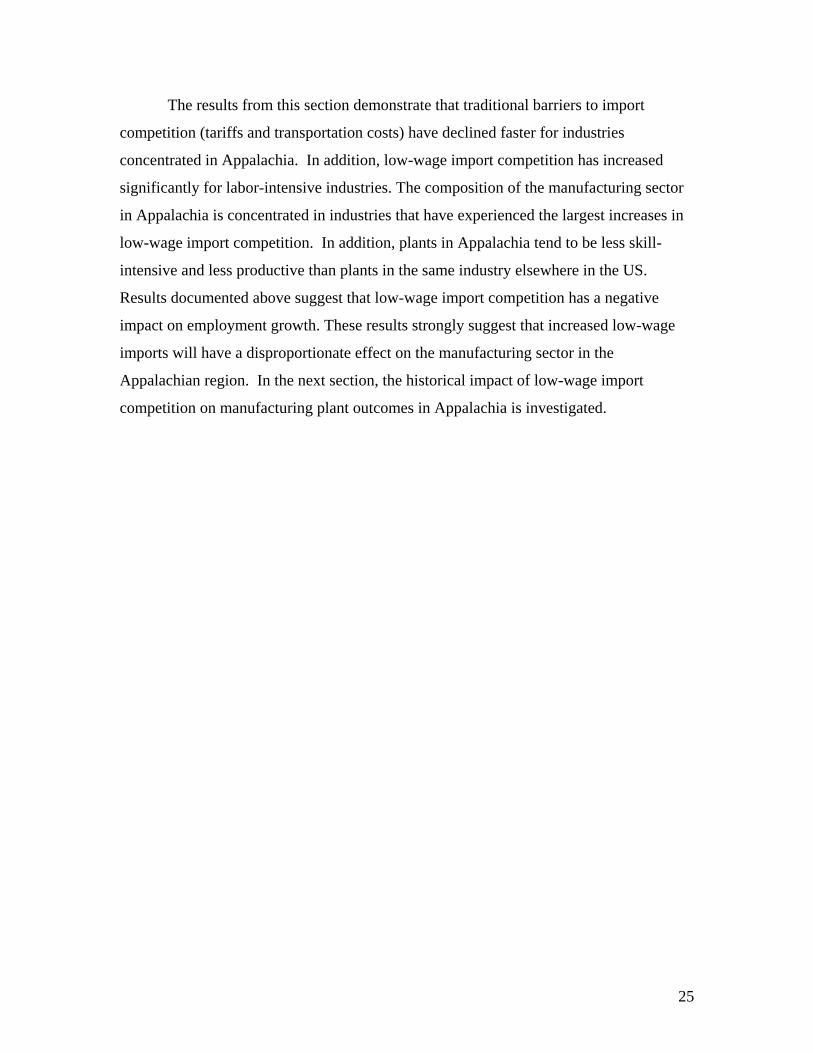
Table 13 highlights differences in low-wage country import shares across regions

within Appalachia over time. These numbers highlight the intra-regional differences in

exposure to low-wage imports. While Appalachia as a whole has higher exposure to low-

wage imports, this is driven entirely by the South region. In 1977, the South region had

low wage import shares more than three times higher than the national average or than

the Appalachian region as a whole. The North region has consistently had an industry

mix that is less exposed to low-wage competition than the ROUS (though the gap is

closing) while the low-wage exposure of the Central region has closely tracked that of the

ROUS.

Table 13: Average Low-Wage Country Exposure by Region and Year

Geographic Area 1977 1982 1987 1992 1997Rest of United States 2.5 2.9 3.8 5.4 9.2Appalachia (Aggregate) 3.0 4.1 5.2 6.8 9.6 North 1.4 1.9 2.8 4.0 6.6 Central 2.4 3.2 4.9 7.8 8.2 South 9.2 6.1 8.6 8.8 10.3

Average Share Of Imports From Low-Wage Countries

Notes: The table displays weighted average exposure to low-wage countrycompetition, measured via VSH, across plants in each geographical area usingoutputs as weights. North, central and south refer to sub-regions of Appalachia.

24

The results from this section demonstrate that traditional barriers to import

competition (tariffs and transportation costs) have declined faster for industries

concentrated in Appalachia. In addition, low-wage import competition has increased

significantly for labor-intensive industries. The composition of the manufacturing sector

in Appalachia is concentrated in industries that have experienced the largest increases in

low-wage import competition. In addition, plants in Appalachia tend to be less skill-

intensive and less productive than plants in the same industry elsewhere in the US.

Results documented above suggest that low-wage import competition has a negative

impact on employment growth. These results strongly suggest that increased low-wage

imports will have a disproportionate effect on the manufacturing sector in the

Appalachian region. In the next section, the historical impact of low-wage import

competition on manufacturing plant outcomes in Appalachia is investigated.

25

IV. The Impact of International Competition on Appalachian Manufacturing Plants

This section describes our methodology for estimating how international

competition, particularly competition from low-wage countries, affects Appalachian

manufacturing plants. We also compare these estimates to the impact of international

competition on non-Appalachian manufacturing plants.

IV.A. Data

Manufacturing plant data come from the Longitudinal Research Database (LRD),

a linked version of the Censuses of Manufactures (CM) collected by the US Bureau of

the Census. The sampling unit for the Census is a manufacturing establishment, or plant,

and the sampling frame in each Census year includes detailed information on inputs,

output, and products on all establishments. Regression analysis covers plant outcomes for

four panels: 1977 to 1982, 1982 to 1987, 1987 to 1992, and 1992 to 1997.

From the Census, we construct plant characteristics including the total value of

shipments, total employment, total capital stock (K, the book value of machinery,

equipment, and buildings) and the quantity of and the wages paid to non-production (N)

and production (P) workers in each Census year. Plant output is recorded at the four-digit

SIC level of aggregation, which is our definition of industry. Plant failure (alternately

plant death or plant shutdown) is defined as the cessation of operations of the plant and

represents a ‘true’ death, i.e. plants that merely change owners between Census years

remain in the sample.

In constructing our sample, we make several modifications to the basic data. First,

while the LRD does contain limited information on very small plants (so-called

Administrative records), we do not include these records in this study due to the lack of

information on inputs other than total employment. Second, we drop any industry whose

products are categorized as ‘not elsewhere classified’ because these ‘industries’ are

typically catch all categories for relatively heterogeneous products. In practice, this

corresponds to any industry whose four-digit code ends in ‘9’. This reduces the number

of industries in the sample to 337. Finally, we drop any manufacturing establishment that

26

does not report one of the required input or output measures. We are left with roughly

443,000 observations encompassing roughly 245,000 plants in the four panels.

As suggested in our analysis above, two input intensities can be observed in the

LRD. Plant capital intensity is measured as the log of the ratio of plant capital stock to

plant production workers. Skill intensity is harder to measure as there is relatively little

information in the LRD on the characteristics of the workforce. We measure plant skill

intensity as the non-production worker wage bill to production worker wage bill.

Beyond the detailed input and output data available on the LRD that enable us to

characterize the input intensities and productivity of individual plants, the LRD also

contains detailed, county level location information for each plant. The county level

information allows us to reliably identify all plants in the Appalachian Regional

Commission region.

It is possible for firms to survive exposure to low-wage countries via productivity

improvements. As a result, we control for plant total factor productivity (TFP ) in our

empirical analysis. As is well known, accurately measuring a plant’s multi-factor

productivity is quite difficult, and we are constrained here in our choice of productivity

measures because we have only single observations for many of the establishments in our

sample. We measure TFP as the residual of a five-input production function for each

industry and year, where the inputs are two types of capital, two types of labor and

purchased inputs. By construction the measure is mean zero for each industry in each

period. We recognize this procedure’s inability to control for the co-movement of

markups and productivity, or the co-movements of variable inputs and productivity. We

note that our reported results are robust to using plant TFP estimates generated from

Bartelsman et al. (2000) industry cost shares. We also note that the relationship we find

between plant outcomes and exposure to low-wage countries is robust to omitting TFP

from all specifications.

IV.B Model

We relate plant outcomes between years t and t + 5 are related to a set of plant

characteristics, the average import share of low-wage countries in the preceding five

27

years, and interactions of plant input intensities and productivity with the measures of

trade costs and low-wage competition,

Outcomet:t+5,p = f (Zpt, Git, Xipt).

where outcomes are plant shutdowns and employment growth. Zpt is a vector of plant

characteristics at time t, Git is a vector of industry-level measures of globalization, and

Xipt is a vector of interactions between plant characteristics and industry globalization

measures. We relate the levels of plant and industry characteristics in year t to changes in

plant outcomes across Census years t to t+5 to mitigate the endogeneity of

contemporaneous behavior and plant characteristics.

We consider two types of plant outcomes. The first is plant death, which we

estimate via probit. The additional plant outcome we consider is the change in plant

employment, which we estimate by OLS. We measure plant employment growth using

log differences which limits our sample to surviving plants. Because we cannot observe

the characteristics of plants prior to their birth, we are unable to include birth

observations in our empirical specifications above.

Our set of plant characteristics encompasses log total employment, age, log TFP,

log capital intensity, and the non-production worker to production worker wage bill ratio.

We use the wage bill ratio in our regressions rather than the percent of skilled workers in

employment reported above to account for unobserved skill variation across plants and

regions (Bernard, Redding and Schott 2005). Our inclusion of controls for plant size

(total employment) and plant age is motivated by the empirical work of Dunne et al.

(1988, 1989) and subsequent theoretical models by Hopenhayn (1992a,b), Olley and

Pakes (1996) and others. The specification also includes time fixed effects, industry or

plant fixed effects are also added to some specifications. Plant output is deflated with

industry shipment deflators available in the NBER Productivity Database compiled by

Bartelsman et al. (2000).

28

IV.C Results

Estimation results presented in Table 14 demonstrate that manufacturing plants in

the Appalachian region are more responsive to low-wage imports than plants elsewhere

in the country. The coefficient on VSH in the plant shutdowns specification (without

including the interaction of VSH with plant characteristics) is about double the

coefficient on VSH for the rest of the country, 0.279 compared to 0.138. The implication

of these results is that a 10-percentage point increase in VSH is associated with an

increase in the probability of plant shutdown by about 1.96 percentage points in

Appalachia (the average probability of a plant closing is about 25 percent). The increase

in probability of plant closure associated with a 10-percentage point increase in VSH in

the ROUS is only 1.09 percentage points. These results suggest that plants in Appalachia

have significantly larger shutdown responses to changes in low-wage import shares than

plants elsewhere in the country.

When the interaction term is included, the difference is smaller. In examining the

interaction between plant characteristics and VSH, capital intensity mitigates the impact

of low-wage import competition. Plants that have higher capital intensity relative to other

plants in their industry are more likely to survive in both the ROUS and Appalachia. In

Appalachia, plants that pay a higher share of wages to non-production (skilled) workers

are also statistically significantly less likely to shutdown.

The employment growth specifications also demonstrate low-wage import shares

have a greater impact on plants in Appalachia than elsewhere in the country. The

coefficient on VSH for the Appalachian sample, in both specifications, is more than

double the rest of US coefficient, -0.053 compared to –0.019 in the specification without

the plant characteristic interactions. This suggests a significantly greater employment

response to low-wage import competition in Appalachia than in the rest of the US. A 10-

percentage point increase in VSH in Appalachia is associated with a decrease in

annualized employment growth by 1.39 percentage points; in the ROUS the marginal

impact is 0.19 percentage points. These results indicate that the employment response is

significantly larger at plants in Appalachia than elsewhere in the country.

29

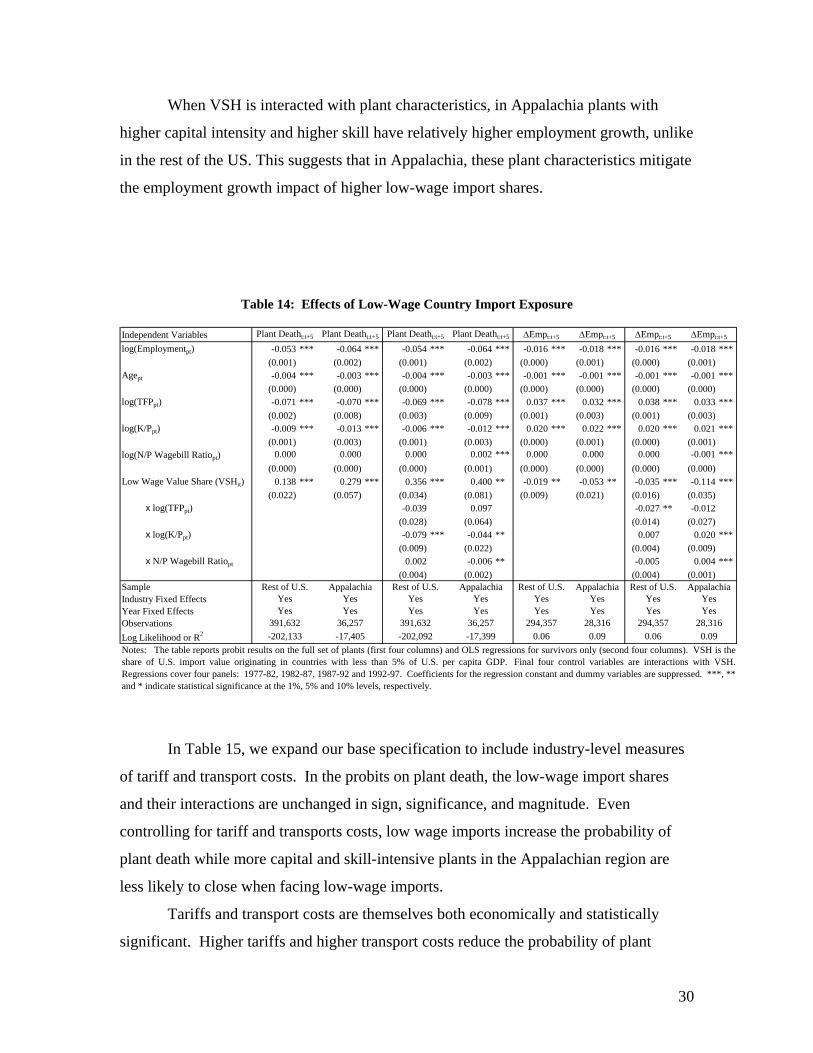
When VSH is interacted with plant characteristics, in Appalachia plants with

higher capital intensity and higher skill have relatively higher employment growth, unlike

in the rest of the US. This suggests that in Appalachia, these plant characteristics mitigate

the employment growth impact of higher low-wage import shares.

Table 14: Effects of Low-Wage Country Import Exposure

Independent Variableslog(Employmentpt) -0.053 *** -0.064 *** -0.054 *** -0.064 *** -0.016 *** -0.018 *** -0.016 *** -0.018 ***

(0.001) (0.002) (0.001) (0.002) (0.000) (0.001) (0.000) (0.001)Agept -0.004 *** -0.003 *** -0.004 *** -0.003 *** -0.001 *** -0.001 *** -0.001 *** -0.001 ***

(0.000) (0.000) (0.000) (0.000) (0.000) (0.000) (0.000) (0.000)log(TFPpt) -0.071 *** -0.070 *** -0.069 *** -0.078 *** 0.037 *** 0.032 *** 0.038 *** 0.033 ***

(0.002) (0.008) (0.003) (0.009) (0.001) (0.003) (0.001) (0.003)log(K/Ppt) -0.009 *** -0.013 *** -0.006 *** -0.012 *** 0.020 *** 0.022 *** 0.020 *** 0.021 ***

(0.001) (0.003) (0.001) (0.003) (0.000) (0.001) (0.000) (0.001)log(N/P Wagebill Ratiopt) 0.000 0.000 0.000 0.002 *** 0.000 0.000 0.000 -0.001 ***

(0.000) (0.000) (0.000) (0.001) (0.000) (0.000) (0.000) (0.000)Low Wage Value Share (VSHit) 0.138 *** 0.279 *** 0.356 *** 0.400 ** -0.019 ** -0.053 ** -0.035 *** -0.114 ***

(0.022) (0.057) (0.034) (0.081) (0.009) (0.021) (0.016) (0.035) x log(TFPpt) -0.039 0.097 -0.027 ** -0.012

(0.028) (0.064) (0.014) (0.027) x log(K/Ppt) -0.079 *** -0.044 ** 0.007 0.020 ***

(0.009) (0.022) (0.004) (0.009) x N/P Wagebill Ratiopt 0.002 -0.006 ** -0.005 0.004 ***

(0.004) (0.002) (0.004) (0.001)SampleIndustry Fixed EffectsYear Fixed EffectsObservationsLog Likelihood or R2

Rest of U.S. Appalachia Rest of U.S. Appalachia

-17,399

Rest of U.S. Appalachia Rest of U.S. Appalachia

YesYes

Notes: The table reports probit results on the full set of plants (first four columns) and OLS regressions for survivors only (second four columns). VSH is theshare of U.S. import value originating in countries with less than 5% of U.S. per capita GDP. Final four control variables are interactions with VSH.Regressions cover four panels: 1977-82, 1982-87, 1987-92 and 1992-97. Coefficients for the regression constant and dummy variables are suppressed. ***, **and * indicate statistical significance at the 1%, 5% and 10% levels, respectively.

YesYes

36,257-17,405

YesYes

28,3160.09-202,133 0.06 0.06 0.09

391,632 294,357 294,357 28,316391,632-202,092

36,257Yes Yes YesYes YesYes Yes YesYes Yes

Plant Deatht:t+5 ΔEmpt:t+5 ΔEmpt:t+5 ΔEmpt:t+5Plant Deatht:t+5 ΔEmpt:t+5Plant Deatht:t+5 Plant Deatht:t+5

In Table 15, we expand our base specification to include industry-level measures

of tariff and transport costs. In the probits on plant death, the low-wage import shares

and their interactions are unchanged in sign, significance, and magnitude. Even

controlling for tariff and transports costs, low wage imports increase the probability of

plant death while more capital and skill-intensive plants in the Appalachian region are

less likely to close when facing low-wage imports.

Tariffs and transport costs are themselves both economically and statistically

significant. Higher tariffs and higher transport costs reduce the probability of plant

30

shutdown and have much larger effects for plants in the Appalachian region than for

those in the ROUS.

The results for surviving plant employment growth are again robust to the

inclusion of the additional trade measures. Employment growth is lower in the face of

low-wage competition and the effect is larger in the Appalachian region. Again within

industries, high-skill and capital-intensive plants are able to offset some of the effects of

low-wage imports. Tariffs and transport costs themselves are positively associated with

employment growth and their effects are strongest in Appalachia.

31

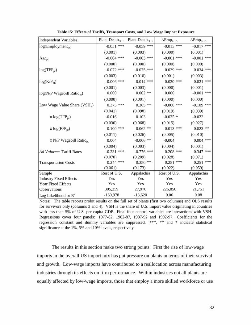
Table 15: Effects of Tariffs, Transport Costs, and Low Wage Import Exposure

Independent Variableslog(Employmentpt) -0.051 *** -0.059 *** -0.015 *** -0.017 ***

(0.001) (0.003) (0.000) (0.001)Agept -0.004 *** -0.003 *** -0.001 *** -0.001 ***

(0.000) (0.000) (0.000) (0.000)log(TFPpt) -0.072 *** -0.075 *** 0.039 *** 0.034 ***

(0.003) (0.010) (0.001) (0.003)log(K/Ppt) -0.006 *** -0.014 *** 0.020 *** 0.021 ***

(0.001) (0.003) (0.000) (0.001)log(N/P Wagebill Ratiopt) 0.000 0.002 ** 0.000 -0.001 ***

(0.000) (0.001) (0.000) (0.000)Low Wage Value Share (VSHit) 0.375 *** 0.365 ** -0.060 *** -0.109 ***

(0.041) (0.098) (0.019) (0.039) x log(TFPpt) -0.016 0.103 -0.025 * -0.022

(0.030) (0.068) (0.015) (0.027) x log(K/Ppt) -0.100 *** -0.062 ** 0.013 *** 0.023 **

(0.011) (0.026) (0.005) (0.010) x N/P Wagebill Ratiopt 0.004 -0.006 ** -0.004 0.004 ***

(0.004) (0.003) (0.004) (0.001)Ad Valorem Tariff Rates -0.231 *** -0.776 *** 0.208 *** 0.347 ***

(0.070) (0.209) (0.028) (0.071)Transportation Costs -0.244 *** -0.356 ** 0.251 *** 0.251 ***

(0.061) (0.173) (0.022) (0.059)SampleIndustry Fixed EffectsYear Fixed EffectsObservationsLog Likelihood or R2

ΔEmpt:t+5 ΔEmpt:t+5Plant Deatht:t+5 Plant Deatht:t+5

Rest of U.S. AppalachiaRest of U.S. AppalachiaYes YesYes YesYes YesYes Yes

226,850 21,751305,259 27,970

Notes: The table reports probit results on the full set of plants (first two columns) and OLS resultsfor survivors only (columns 3 and 4). VSH is the share of U.S. import value originating in countrieswith less than 5% of U.S. per capita GDP. Final four control variables are interactions with VSH.Regressions cover four panels: 1977-82, 1982-87, 1987-92 and 1992-97. Coefficients for theregression constant and dummy variables are suppressed. ***, ** and * indicate statisticalsignificance at the 1%, 5% and 10% levels, respectively.

0.06 0.08-160,978 -13,620

The results in this section make two strong points. First the rise of low-wage

imports in the overall US import mix has put pressure on plants in terms of their survival

and growth. Low-wage imports have contributed to a reallocation across manufacturing

industries through its effects on firm performance. Within industries not all plants are

equally affected by low-wage imports, those that employ a more skilled workforce or use

32

capital intensively have been able to avoid some of the competition from low-wage

countries.

Second, the effects of low-wage imports have been greater for plants within the

Appalachian region both in terms of the level of exposure they face and the response to

that exposure. For comparable low-wage import share, Appalachian plants show higher

probabilities of closure and lower employment growth for survivors. However, within-

industries skill and capital-intensity play a larger role in insulating Appalachian plants

from low-wage imports.

The results above suggest that Appalachian manufacturing is more exposed to

low-wage import shares and has a greater response to low-wage competition than the rest

of the US. We now turn our focus to the expected trends of these international factors in

the future and the likely responses by firms and industries in the US manufacturing sector

as a whole and in the Appalachian region in particular.

33

V. The Future Evolution of Low-Wage Imports, Tariff and Transportation Costs

Given the important influences of low-wage country import shares, tariffs and

transports on the path of Appalachian manufacturing, it is useful to examine how they

will evolve in the coming years. We introduce a method for forecasting industry low-

wage import shares. To formulate this forecast, we take advantage of the fact that low-

wage country product penetration today is a good predictor of low-wage import market

share in the future (Bernard et al 2004b). For transport costs, tariffs and other trade

policies we discuss likely developments over the next decade.

V.A. Low-Wage Imports Going Forward

Analysis of product-level trade data indicates that low-wage country market entry

patterns have been quite consistent over time. Firms from low-wage countries first enter a

US industry by selling relatively small amounts of relatively low value products. They

next expand the breadth of their offerings to cover most of the products in an industry.

Finally, they boost the quantity, and therefore value, of each product. This path of initial

entry and subsequent expansion of volume culminates in a dramatic rise in the share of

industry imports sourced from low-wage countries. Figure 6 plots both the share of

aggregate manufacturing import value imported from low-wage countries as well as the

low-wage countries’ breadth of product penetration. We define the low-wage countries’

product penetration as the share of products in an industry sourced from low-wage

countries (referred to as number share or NSH which represents the number of products

in an industry imported from low wage countries relative to the total number of products

imported in an industry).9 The product penetration can range from zero to one, with one

indicating that all of the products in an industry are imported from low-wage countries.

Comparison of the two lines in the figure indicates that import value share lags its

product penetration by about a decade: the rise in penetration beginning in 1978 is

followed by a noticeable rise in value share starting in 1988. 9 In the US trade data, products are defined according to ten-digit Harmonized System code, known as HS codes. On average, there are 622 products in each of the 20 manufacturing industries listed in Table 16.

34

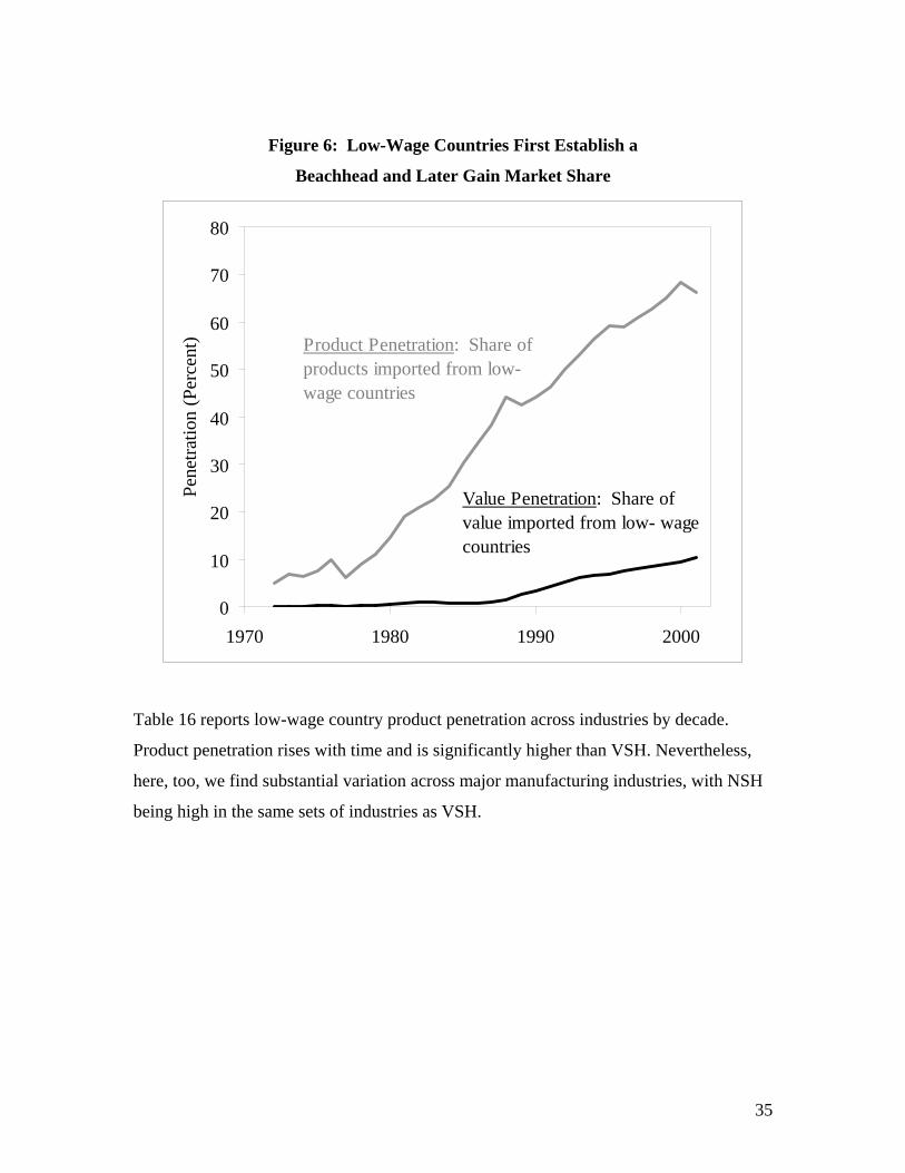
Figure 6: Low-Wage Countries First Establish a

Beachhead and Later Gain Market Share

0

10

20

30

40

50

60

70

80

1970 1980 1990 2000

Pene

tratio

n (P

erce

nt) Product Penetration: Share of

products imported from low- wage countries

Value Penetration: Share of value imported from low- wage countries

Table 16 reports low-wage country product penetration across industries by decade.

Product penetration rises with time and is significantly higher than VSH. Nevertheless,

here, too, we find substantial variation across major manufacturing industries, with NSH

being high in the same sets of industries as VSH.

35

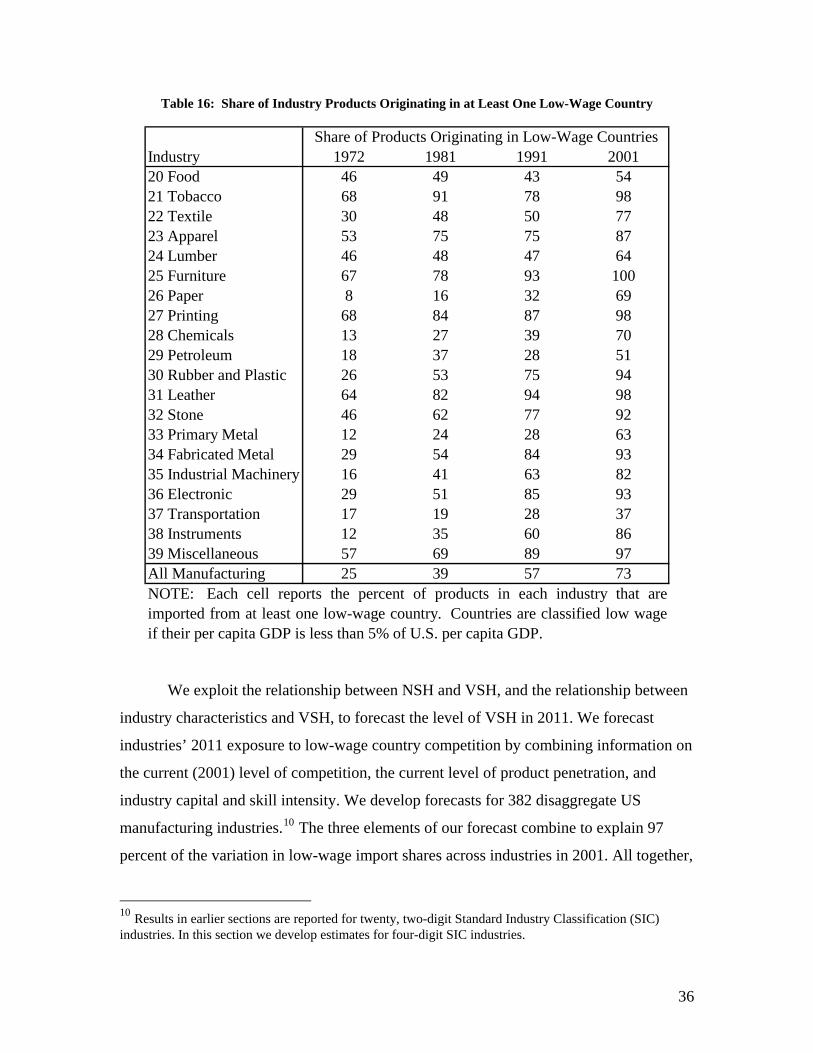
Table 16: Share of Industry Products Originating in at Least One Low-Wage Country

Industry 1972 1981 1991 200120 Food 46 49 43 5421 Tobacco 68 91 78 9822 Textile 30 48 50 7723 Apparel 53 75 75 8724 Lumber 46 48 47 6425 Furniture 67 78 93 10026 Paper 8 16 32 6927 Printing 68 84 87 9828 Chemicals 13 27 39 7029 Petroleum 18 37 28 5130 Rubber and Plastic 26 53 75 9431 Leather 64 82 94 9832 Stone 46 62 77 9233 Primary Metal 12 24 28 6334 Fabricated Metal 29 54 84 9335 Industrial Machinery 16 41 63 8236 Electronic 29 51 85 9337 Transportation 17 19 28 3738 Instruments 12 35 60 8639 Miscellaneous 57 69 89 97All Manufacturing 25 39 57 73

Share of Products Originating in Low-Wage Countries

NOTE: Each cell reports the percent of products in each industry that areimported from at least one low-wage country. Countries are classified low wageif their per capita GDP is less than 5% of U.S. per capita GDP.

We exploit the relationship between NSH and VSH, and the relationship between

industry characteristics and VSH, to forecast the level of VSH in 2011. We forecast

industries’ 2011 exposure to low-wage country competition by combining information on

the current (2001) level of competition, the current level of product penetration, and

industry capital and skill intensity. We develop forecasts for 382 disaggregate US

manufacturing industries.10 The three elements of our forecast combine to explain 97

percent of the variation in low-wage import shares across industries in 2001. All together,

10 Results in earlier sections are reported for twenty, two-digit Standard Industry Classification (SIC) industries. In this section we develop estimates for four-digit SIC industries.

36

each factor has the expected relationship: high competition today is a solid predictor of

high competition in ten years; product penetration today is a reliable signal of where low-

wage competition will concentrate in the future; and industries that use more capital and

skill in production face less competition in ten years.

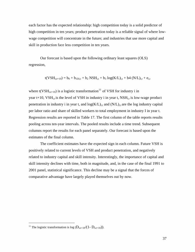
Our forecast is based upon the following ordinary least squares (OLS)

regression,

t(VSHi,t+10) = b0 + b1Di,t + b2 NSHi,t + b3 log(K/L)i,t + b4 (N/L)i,t + ei,t

where t(VSHi,t+10) is a logistic transformation11 of VSH for industry i in

year t+10, VSHi,t is the level of VSH in industry i in year t, NSHi,t is low-wage product

penetration in industry i in year t, and log(K/L)i,t and (N/L)i,t are the log industry capital

per labor ratio and share of skilled workers to total employment in industry I in year t.

Regression results are reported in Table 17. The first column of the table reports results

pooling across ten-year intervals. The pooled results include a time trend. Subsequent

columns report the results for each panel separately. Our forecast is based upon the

estimates of the final column.

The coefficient estimates have the expected sign in each column. Future VSH is

positively related to current levels of VSH and product penetration, and negatively

related to industry capital and skill intensity. Interestingly, the importance of capital and

skill intensity declines with time, both in magnitude, and, in the case of the final 1991 to

2001 panel, statistical significance. This decline may be a signal that the forces of

comparative advantage have largely played themselves out by now.

11 The logistic transformation is log (Di,t+10/(1- Di,t+10)).

37

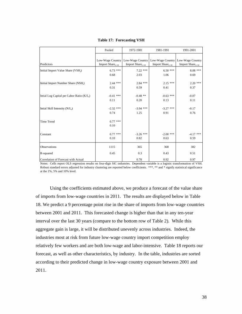
Table 17: Forecasting VSH

Predictors

Initial Import Value Share (VSHt) 6.73 *** 7.22 *** 6.50 *** 8.08 ***0.68 2.03 1.06 0.69

Initial Import Number Share (NSHt) 2.44 *** 2.84 *** 2.15 *** 2.20 ***0.31 0.59 0.41 0.37

Intial Log Capital per Labor Ratio (K/Lt) -0.41 *** -0.48 ** -0.63 *** -0.070.11 0.20 0.13 0.11

Intial Skill Intensity (N/Lt) -2.32 *** -3.94 *** -3.27 *** -0.170.74 1.25 0.91 0.76

Time Trend 0.77 ***0.10

Constant 0.77 *** -3.26 *** -2.00 *** -4.17 ***0.10 0.82 0.63 0.59

Observations 1115 365 368 382

R-squared 0.45 0.3 0.43 0.51

Correlation of Forecast with Actual 0.78 0.92 0.97

Pooled

Low-Wage Country Import Sharet+10

1991-2001

Low-Wage Country Import Sharet+10

1972-1981

Low-Wage Country Import Sharet+10

1981-1991

Low-Wage Country Import Sharet+10

Notes: Cells report OLS regression results on four-digit SIC industries. Dependent variable is a logistic transformation of VSH.Robust standard errors adjusted for industry clustering are reported below coefficients. ***, ** and * signify statistical significanceat the 1%, 5% and 10% level.

Using the coefficients estimated above, we produce a forecast of the value share

of imports from low-wage countries in 2011. The results are displayed below in Table

18. We predict a 9 percentage point rise in the share of imports from low-wage countries

between 2001 and 2011. This forecasted change is higher than that in any ten-year

interval over the last 30 years (compare to the bottom row of Table 2). While this

aggregate gain is large, it will be distributed unevenly across industries. Indeed, the

industries most at risk from future low-wage country import competition employ

relatively few workers and are both low-wage and labor-intensive. Table 18 reports our

forecast, as well as other characteristics, by industry. In the table, industries are sorted

according to their predicted change in low-wage country exposure between 2001 and

2011.

38

Four sectors – Leather Goods, Apparel, Furniture and Miscellaneous – are

forecast to experience increases in low-wage country import shares of more than 20

percentage points by 2011. These industries pay below-average wages and have a small

share of US manufacturing employment, yet are relatively important in the Appalachian

region.

Table 18: Forecasted Change in US Exposure to Low-Wage Country Imports, 2001 to 2011

Employment HourlyIndustry 2001 2011 Change Emp Share Wage ($)31 Leather Goods 61 87 26 0.3 1023 Apparel 41 67 25 3.2 925 Furniture 33 57 24 2.9 1239 Misc (e.g. Toys) 43 65 22 2.1 1232 Stone & Concrete 22 36 14 3.2 1534 Fabricated Metal 17 30 13 8.4 1427 Printing 19 31 13 8.4 1530 Plastic & Rubber 30 42 12 5.4 1322 Textiles 22 32 10 2.7 1136 Electronics 18 28 10 9.2 1424 Lumber 10 19 8 4.4 1226 Paper 7 14 7 3.6 1635 Industrial Machinery 12 19 6 11.4 1638 Instruments 9 15 6 4.7 1537 Trans Equip 1 4 3 9.9 1920 Food 8 11 3 9.6 1328 Chemicals 4 7 2 5.8 1833 Primary Metal 6 7 2 3.7 1629 Petroleum 7 5 -2 0.7 21

All Manufacturing 15 24 9 100.0 14

Low-Wage Import Share

Notes: Industry identifiers are preceded by their two-digit Standard Industrial Classification(SIC) code. Rows are sorted by forecast change in low-wage country import share between2001 and 2011 (column 4). The employment share is the fraction of U.S. manufacturingemployment in the sector in 2001. The hourly wage is the average nominal hourly wage in thesector in 2001. Employment and wage data are from the U.S. Bureau of Labor statisticsavailable at www.bls.gov.

The combination of concentration in labor-intensive sectors, the relatively large

response to low-wage imports in Appalachia, and the forecast for significant growth in

39

VSH in sectors important in Appalachia suggest that import competition will pose an

important challenge to the region.

V.B. Transportation Costs Going Forward

Over the last 30 years, transportation costs have fallen substantially across a broad

range of products. However, events in recent years have called into question the

perpetuation of such a downward trend in transport costs and might even foreshadow a

period of globally higher freight costs. Both the sustained rise in energy prices and, in

particular, the huge increase in import demand in China has combined to put upward

pressure on transport prices in the short run.12

Over longer horizons, reasonable forecasts of freight and insurance costs are

relatively flat, however such expectations come complete with large standard deviations.

The next decade is likely to see flat transport costs but scenarios with large increases or

modest declines are possible.

V.C. Tariffs and the Trade Policy Environment Going Forward

As reported in Table 5, tariffs have decreased significantly over the last 30 years

and are currently very low in most sectors. Since tariff changes are typically the by-

product of multilateral or bilateral negotiations or under direct political control, we are

unable to produce estimates of tariff changes by sector going forward. Instead we

consider the prospects of the major ongoing trade negotiations and their likely effect on

tariffs and trade openness in general.

12 See the Beige Book Summary of Commentary on Current Economic Conditions by Federal Reserve District, March 3, 2004 Federal Reserve Board of Governors.

40

V.C.1 Overall Environment

The current environment – both political and economic – provides limited

prospects for additional liberalization in the near-term. On the political side, a wide range

of polls suggest that the electorate is evenly split or against further liberalization of trade

policies (see Slaughter and Scheve ((2001)). This sentiment is evident in the Congress.

The limited political mandate seems to be reflected in narrow and partisan House votes

approving Trade Promotion Authority in 2001 and 2002 and increasing partisanship on

trade issues in general. The narrow support and voting margins for trade policy increase

the ability of special interests to block further liberalization.

On the economic side, the US current account deficit is at historical highs – both

in absolute terms and as a share of GDP. High trade deficits typically mitigate against

trade liberalization. There is also a broad-based perception that the US dollar is over-

valued relative to other currencies. This also tends to increase protectionist pressure (as

evidenced by recently proposed legislation and a number of requests from specific

industries for special protections from trade with China). The sluggishness in

employment growth (and the related debate on outsourcing and jobs) is also likely to

dampen enthusiasm for trade liberalization.

In spite of the issues discussed above, the US is currently pursuing a broad array

of trade policy initiatives, including the Doha Round in the WTO, the Free Trade Area of

the Americas negotiation with other countries in the western hemisphere, and a number

of bilateral Free Trade Agreements.

V.C.2 Doha Round in the WTO

The Doha Round of negotiations in the WTO, launched in November 2001 and

originally scheduled to be completed in January 2005, is behind schedule. After the failed

ministerial meeting in Cancun in 2003, the distance between members’ positions

particularly between the developing countries and the developed countries on agricultural

sector issues was evident. It was not clear (and still is not) that the Doha Round will come

to a successful conclusion. To achieve a successful Doha Round, both developing and

41

developed countries will need to make significant (and difficult) changes in their

domestic agricultural programs and agricultural market access. Negotiators worked hard

to get the negotiations back on track and in the July 2004 meeting in Geneva, WTO

members agreed on new guidelines for the negotiation of global trade reforms in

agriculture, manufactured goods, and services. In the meeting, members also agreed to

launch new negotiations on trade procedures and customs reform and to delete the other

“Singapore issues” on how countries treat foreign direct investment in their countries,

how countries manage their competition or anti-trust policy, and the process by which

countries governments’ procure goods and services.

The ambitious US proposal to eliminate tariffs on industrial goods by 2015 seems

unlikely to be accepted, as there is resistance in both the US and in some developing

countries. The major developments in the Doha Round are likely to be reducing barriers

for agricultural product imports in developing countries and reducing barriers for

industrial products and services in developing (particularly middle-income) countries.

The next WTO ministerial in Hong Kong in December 2005 will be key to a

successful conclusion of the round. A key milestone in concluding the negotiation is

likely to be the expiration of Trade Promotion Authority in June 2007 (assuming it is

reauthorized by Congress in 2005). Thus, it is unlikely that the Doha Round will be

complete before mid-2007, if at all.

The most likely outcome for tariffs on manufactured products from low-wage

countries is a relative absence of change or movement towards reduction. This suggests

that there will be little multilateral downward pressure on tariff rates over the medium

term.

V.C.3 Free Trade Area of the Americas

Similar to the Doha Round in the WTO, the FTAA negotiations are not

proceeding well. The FTAA ministerial meeting in Miami in November 2003 achieved

little more than papering over the differences between the negotiators. The prospect of

“FTAA-lite,” that the Miami meeting suggested, would allow countries to exclude certain

sensitive areas from reform. This prospect significantly reduces the prospect of achieving

42

an ambitious and comprehensive trade reform package. The talks are currently well

behind schedule and are likely to proceed in parallel with the Doha Round for the next

two years. The FTAA does not present significant promise of additional trade

liberalization in the near-term. Even if the FTAA were to come to successful fruition,

only Haiti, Honduras, and Nicaragua are low-wage countries by our definition, so it

seems unlikely that the FTAA would accelerate the rate of growth in low-wage imports.

It is perhaps more likely that preferential access for Central and South America will

divert some trade from low-wage Asian countries to higher income Central and South

American countries.

V.C.4 Bilateral Free Trade Agreements

In part because of the issues with the Doha Round in the WTO and the difficulties

in the FTAA negotiations, the US is pursuing a number of bilateral or regional Free Trade

Agreements (FTA).

The US currently has FTAs with Canada, Mexico, Chile, Singapore, Jordan,

Israel, Australia, and Morocco. There are three agreements that are subject to ratification,

Bahrain, and CAFTA (Costa Rica, Honduras, El Salvador, Guatemala, and Nicaragua and

the Dominican Republic). Similar to the FTAA, the current list of FTA agreements and

pending agreements include only a small number of low-wage countries (Haiti and

Honduras), so it seems unlikely that CAFTA or the other bilaterals would accelerate the

rate of growth in low-wage imports.13 It is perhaps more likely that preferential access for

Central and South America will divert some trade from low-wage Asian countries to

higher income Central and South American countries.

The US is pursuing negotiations with Colombia, Ecuador, Peru, Panama,

Thailand, and the South Africa Customs Union (Botswana, Lesotho, Namibia, South

Africa and Swaziland). These countries are not low-wage countries, so these trade

agreements, if realized, are unlikely to increase the rate of growth of imports from low-

13 At this point in time, it is still difficult to predict whether the CAFTA agreement will be ratified by the Congress.

43

wage countries. They are more likely to divert trade from low-wage countries in the near-

term.

V.C.5 Expiration of the Multi-Fiber Arrangement

The other looming development on the trade policy front is the expiration of the

Multi-Fiber Arrangement (MFA), which expired in January 2005. The MFA has

controlled trade in textiles and apparel for more than 40 years. Many analysts expect that

with the expiration of the MFA, a significant share of the world’s textile and apparel

production will shift to China and other low-wage producers – displacing employment in

both developed countries and developing non-Asian countries. Consistent with other

analyses, our forecast shows a significant increase in the low-wage country share of

textiles and apparel.

There are a number of policy developments that might moderate the growth in

low-wage textile and apparel imports – specifically imports from China – including a

China-specific Textile Safeguard remedy, regular safeguard measures, and standard anti-

dumping measures.14

While it is difficult to forecast the reaction of a future US administration, in 2003

the US Department of Commerce imposed a 7.5 percent quota limit on the growth of

Chinese bra, knit fabric, dressing gown, and robe imports above the levels reached

between September 2002 and September 2003. Current Administration officials have

indicated in press interviews that they will consider using the safeguard provisions

available to it under the WTO agreement to prevent “market disruption” in other textile

and apparel goods.15 These safeguard and anti-dumping responses are likely to moderate

the growth of textile and apparel imports from China.

14 Hufbauer and Wong (2004) describe the range of policy alternatives the US government has at its disposal to limit the increase in imports from China. 15 “US May Limit Chinese Imports” by Peter S. Goodman, Washington Post, September 13, 2004.

44

VI. Going Forward – 3 Scenarios

The results presented above lead to the immediate conclusion that the rise in

imports from low wage countries has played a large role in shaping the face of US

manufacturing in general and in the Appalachian region in particular over the last 30

years. In this section we present three scenarios for the next decade based on the

forecasts of low wage imports and the possible paths for trade policy and transportation

costs.

Scenario 1: The Most Likely Path

We start with the scenario that we consider most likely: one of large increase in

import shares from low-wage countries, modest tariff reductions for most goods with

reactive protection on some specific products, and a general stabilization of freight and

transport costs.

The dominant feature of this scenario is the prospect for increasing import shares

for low-wage countries. There is little doubt that going forward imports from low-wage

countries will continue to rise. Using the results from our model of how low-wage

countries enter US markets, we expect to see a significant rise in low-wage import shares

over the next decade. However, as in the last three decades, there will be substantial

variation by industry in the degree of low-wage import penetration.

In this scenario, sectors that have already had substantial restructuring such as

Apparel and Leather will continue to see rapidly rising imports from low-wage countries.

In addition, sectors such as Furniture will enter a phase of rapid low-wage import growth

and likely find domestic employment and output continuing to fall. These industries have

already undergone a substantial round of adjustment to low-wage imports and while their

prospects in the US are limited, these industries are relatively small and at a national level

the loss of jobs will be relatively muted. However, in regions and communities where the

affected industries represent a significant share of employment, there is potential for

considerable disruption to local labor markets.

45

Manufacturing sectors with the highest wages, greatest employment shares, and

highest productivity will not be subject to massive imports from low-wage countries.

Prospects for domestic production in these industries will be relatively good and some

sub-sectors may even expand employment as the reallocation of activity within

manufacturing continues, helping to foster continued aggregate productivity gains. For

manufacturing as a whole, the employment losses due to low-wage imports will be

modest.

In this most likely scenario, the prospects for large changes in tariff rates or

freight and transport costs are relatively small. The focus of multilateral trade

negotiations is likely to be on areas other than manufacturing and possible bilateral

treaties with countries such as Australia will not lead to large increases in import

volumes. As a result, we foresee no substantive changes in overall tariff levels. On the

other hand, for specific products, such as furniture and apparel, there remains the

possibility of reactive tariff-based protection. We see little chance that such events would

alter the process of reallocation in the manufacturing sector as a whole.

Scenario 1 in the Appalachian Region

The Appalachian region continues to face higher levels of exposure to low-wage

imports, especially in its South region, as shown in Table 13 above. The effects of this

increased exposure is exacerbated by the fact that the process of reallocation in the

manufacturing sector has been lagging in the Appalachian region and the ability of the

region to adjust through changes in firm entry and exit has been lower than that of the

country as a whole. These factors combine to yield slightly more pessimistic predictions

for the manufacturing sector in the Appalachian region.

Figure 7 shows the historical and forecast low-wage import shares for the sub-

regions within the ARC and the rest of the US (the figure uses 1997 shipments as weights

for forecast low-wage country import shares). As can be seen in the figure, the low-wage

import exposure for the region is increasing faster than the ROUS. Even for the North

sub-region, which historically has had lower low-wage import exposure than the ROUS,

the forecast for 2011 shows higher exposure than the ROUS. For the Central sub-region

46

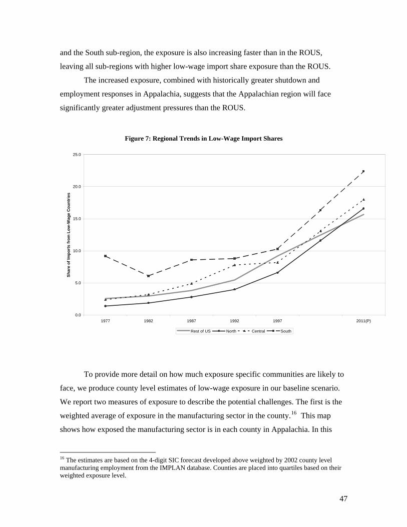
and the South sub-region, the exposure is also increasing faster than in the ROUS,

leaving all sub-regions with higher low-wage import share exposure than the ROUS.

The increased exposure, combined with historically greater shutdown and

employment responses in Appalachia, suggests that the Appalachian region will face

significantly greater adjustment pressures than the ROUS.

Figure 7: Regional Trends in Low-Wage Import Shares

0.0

5.0

10.0

15.0

20.0

25.0

1977 1982 1987 1992 1997 2011(P)

Shar

e of

Impo

rts

from

Low

-Wag

e C

ount

ries

Rest of US North Central South

To provide more detail on how much exposure specific communities are likely to

face, we produce county level estimates of low-wage exposure in our baseline scenario.

We report two measures of exposure to describe the potential challenges. The first is the

weighted average of exposure in the manufacturing sector in the county.16 This map

shows how exposed the manufacturing sector is in each county in Appalachia. In this

16 The estimates are based on the 4-digit SIC forecast developed above weighted by 2002 county level manufacturing employment from the IMPLAN database. Counties are placed into quartiles based on their weighted exposure level.

47

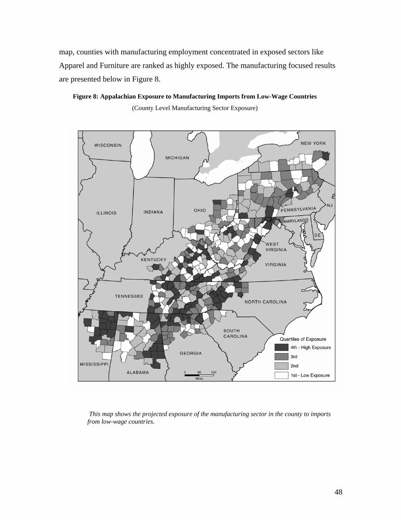
map, counties with manufacturing employment concentrated in exposed sectors like

Apparel and Furniture are ranked as highly exposed. The manufacturing focused results

are presented below in Figure 8.

Figure 8: Appalachian Exposure to Manufacturing Imports from Low-Wage Countries

(County Level Manufacturing Sector Exposure)

This map shows the projected exposure of the manufacturing sector in the county to imports from low-wage countries.

48

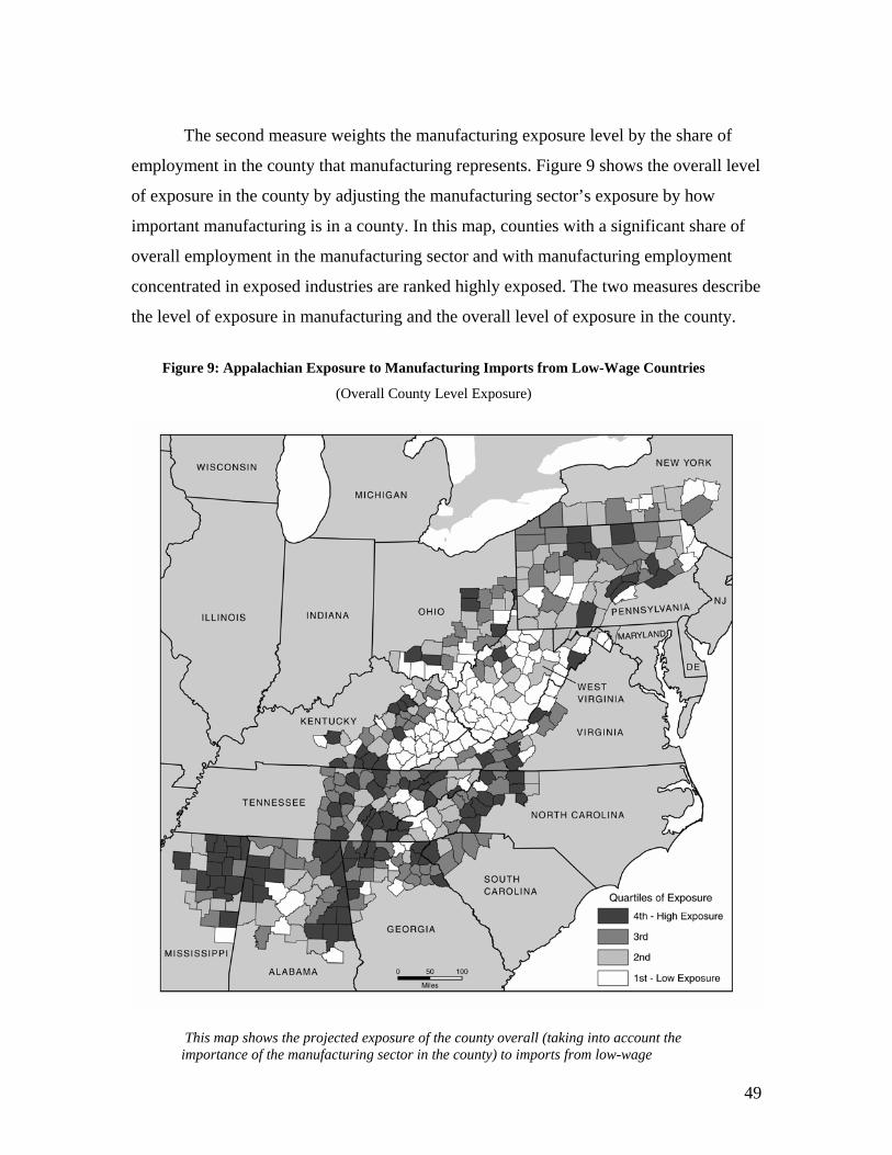
The second measure weights the manufacturing exposure level by the share of

employment in the county that manufacturing represents. Figure 9 shows the overall level

of exposure in the county by adjusting the manufacturing sector’s exposure by how

important manufacturing is in a county. In this map, counties with a significant share of

overall employment in the manufacturing sector and with manufacturing employment

concentrated in exposed industries are ranked highly exposed. The two measures describe

the level of exposure in manufacturing and the overall level of exposure in the county.

Figure 9: Appalachian Exposure to Manufacturing Imports from Low-Wage Countries

(Overall County Level Exposure)

This map shows the projected exposure of the county overall (taking into account the importance of the manufacturing sector in the county) to imports from low-wage

49

Substantial reallocation away from labor-intensive, low-wage sectors will

continue in the region over the next decade. This cross-industry movement will be

coupled with continued reallocation within sectors as the relatively capital-poor plants of

the region face stiffer direct competition from low-wage country imports. Compounding

the problems associated with reallocation is the problem of low firm creation rates across

industries in the region.

Scenario 2: Slowing Globalization

The second scenario is one of modest increases in global economic integration

characterized by low increases in both import volumes and the share of imports from

low-wage countries. In this case, the past trends for all three major factors, low-wage

imports, tariffs, and transport costs, are slowed or reversed. Low-wage import shares

continue to increase but at a slower pace than in the past decade; tariff rates are

unchanged across manufacturing industries; and freight and transport costs rise

substantially due to the increased demands of rapidly growing economies such as China.

While we consider this scenario to be substantially less likely than scenario 1, it remains

a possibility especially as the future of transport costs is highly uncertain and subject to

possible demand pressure and supply constraints.

In this view of the global economy over the next decade, the process of

reallocation in US manufacturing continues but at a slower pace. The slower pace would

have two effects. The slower pace of globalization would provide less pressure on low-

wage labor-intensive industries and firms. However, the slowing pace of globalization

would also constrain the growth of capital and technology-intensive sectors, dampening

output, employment, and productivity growth in these sectors. While slowing

globalization might provide some solace for industries that face higher and increasing

low-wage import shares, for manufacturing as a whole it would mitigate employment

reductions at the expense of lower wage and productivity growth.

50

Scenario 2 in the Appalachian Region

This scenario of slowing global trade growth would affect the Appalachian

Region in one of two different ways. One possibility is that a reduction in the pressure

from low-wage countries would allow firms in low-skill, low-wage industries the time to

reorganize, possibly by shifting to new products, new industries, and new technologies.

However, given the history of lower firm entry and exit in the region, a more

likely long-run outcome would be a perpetuation of the old industrial mix. The ultimate

result of such persistence would be a regional manufacturing base that was ill-prepared to

transform itself going forward and was even more exposed to dislocation from low-wage

imports when the pressure resumed.

Scenario 3: Accelerating Change

In this final scenario, we consider the prospects for US and Appalachian

manufacturing if the global economy expands rapidly and allows for even more rapid

integration and globalization. The key features of this scenario are dramatic

liberalizations in sectors other than manufacturing due to multilateral negotiations, a

continued decline in transport costs, and the rapid emergence of other large low-wage

countries such as India in the global manufacturing production network. We must

emphasize that we see this scenario as the least likely of the three given the current global

economic environment.

With these changes, the share of manufactured imports from low-wage countries

would increase beyond the 25% predicted by our model. However, the distributional

array of such import would not be substantially changed, only the levels would be higher.

The consequences for such events on US firms are quite clear. Pressure in low-wage

industries and for low-tech, labor-intensive producers in all industries would be

magnified, leading to higher exit rates, slower employment growth and greater amounts

of product switching.

However, the obverse side of increasing integration and globalization would mean

greater world-wide opportunities for export-oriented sectors such as transportation, and

51

for skill-intensive sectors in general. Overall, we would expect to see substantially

higher rates of firm turnover, both entry and exit, in a wide variety of industries. This

accelerating reallocation would foster even faster productivity growth.

Scenario 3 in the Appalachian Region

A ramp-up of globalization would have sharp consequences for manufacturing in

the Appalachian region. The composition of Appalachian industries means the region is

unduly exposed to a rapid increase in low-wage imports. In addition, the preponderance

of low-skill, low wage plants means than even in sectors with expansion possibilities, the

Appalachian region would see disproportionate numbers of firm failures and problems

with employment growth.

Of particular concern is the relatively poor performance in firm creation in the

region. Increased globalization and integration place a premium on regions that can

rapidly adjust their firm and industry mix, in particular obsolete enterprises must be

rapidly replaced by new firms in new sectors. The historical record shows that the

Appalachian region is at a disadvantage in this key business performance indicator and

would face significant challenges in this scenario.

52

VII. Summary and Conclusion:

The Appalachian region faces significantly greater challenges from import

competition from low-wage countries than the rest of the US. The challenges come from

the combination of a number of factors.

First, import shares from low-wage countries are forecast to increase significantly

between now and 2011, increasing faster over the period than in any decade over the past

30 years. We develop a forecast of import shares from low-wage countries for 2011 and

demonstrate that import shares from low-wage countries are likely to rise, significantly so

for labor-intensive industries.

Second, manufacturing activity in Appalachia is concentrated in low-wage, labor-

intensive industries that are forecast to experience the greatest increases in low-wage

import competition. Further, even within industries, plants within Appalachia are less

skill-intensive and less productive. Due to the industrial base in Appalachia, the region

overall and all sub-regions are forecast to experience greater increases in low-wage

import shares than the rest of the US, with all regions having higher exposure than the

ROUS in 2011.

Third, in addition to increased exposure, manufacturing plants in Appalachia have

exhibited greater plant shutdown and employment decline responses to low-wage import

competition than the rest of the US. We estimate the responses of manufacturing plants

in Appalachia and the ROUS to increased low-wage import shares and tariffs and

transportation costs. Increased low-wage import shares increase the likelihood of plant

shutdown and decrease relative employment growth in Appalachia and the ROUS, with

the response being greater in Appalachian than the ROUS.

Fourth, a compounding factor is that Appalachia is less dynamic in terms of plant

entry and exit than the rest of the country. As has been documented in other studies, plant

entry and exit rates in Appalachia are lower than the ROUS. This lack of dynamism may

impede the reallocation process in Appalachia and leave the region exposed to low-wage

import competition.

One potentially productive avenue of future research is to examine the sources of

the lower entry and exit rates in Appalachia. Given the current manufacturing base and

53

the forecast for increased low-wage competition, the Region faces the prospect of

significant reallocation. Understanding the impediments to the reallocation process in

Appalachia and developing policies to facilitate adjustment should be important

objectives for policymakers in the Region.

References:

Bartelsman, Eric and Mark Doms, (2000) ‘Understanding Productivity: Lessons from Longitudinal Microdata’, Journal of Economic Literature, XXXVIII, 569-94. Bernard, Andrew B., J. Bradford Jensen and Peter K. Schott. (2004a) ‘Falling Trade Costs, Heterogeneous Firms, and Industry Dynamics’. Tuck School of Business mimeo, revision of NBER Working Paper #9639. Bernard, Andrew B., J. Bradford Jensen and Peter K. Schott. (2004b) ‘Facing The Dragon: Prospects For US Manufacturers in the Coming Decade’. Tuck School of Business mimeo. Bernard, Andrew B., J. Bradford Jensen and Peter K. Schott. (2005) ‘Survival of the Best Fit: Exposure to Low Wage Countries and the (Uneven) Growth of US Manufacturing Plants’. Journal of International Economics, forthcoming. Bernard, Andrew B., Stephen Redding and Peter K. Schott. (2004) ‘Product Choice and Product Switching’. Tuck School of Business mimeo, revision of NBER Working Paper #9789.. Bernard, Andrew B., Stephen Redding and Peter K. Schott. (2005) ‘Factor Price Equality and the Economies of the United States’ Centre for Economic Policy Discussion Paper 5126. Dunne, Timothy, Mark J. Roberts, and Larry Samuelson, (1988) “Patterns of firm entry and exit in US manufacturing industries”, Rand Journal of Economics, Vol. 19(4), 495-515. Dunne, Timothy, Mark J. Roberts, and Larry Samuelson. (1988) ‘The Growth and Failure of US Manufacturing Plants’, Quarterly Journal of Economics, Vol. 104, No. 4 , pp. 671-698. Dunne, Timothy, Mark J. Roberts, and Larry Samuelson. (1989) ‘The Growth and Failure of US Manufacturing Plants’, Quarterly Journal of Economics, Vol. 104, No. 4 , pp. 671-698.

54

Feenstra, Robert C. (1996) ‘US Imports 1972-1994: Data and Concordances.’ NBER Working Paper # 5515. Feenstra, Robert C., John Romalis and Peter K. Schott. (2002) ‘US Imports, Exports, and Tariff Data, 1989-2001’ NBER Working Paper # 9387. Foster, Lucia (2004) ‘The Appalachian Economy, Establishment and Employment Dynamics, 1982-1997: Evidence from the Longitudinal Business Database,’ Appalachian Regional Commission Report. Hufbauer, Gary and Yee Wong, (2004) ‘China Bashing 2004’, Institute for International Economics International Policy Brief PB04-5. Hopenhayn, Hugo. (1992a) ‘Entry, Exit, and Firm Dynamics in Long Run Equilibrium’, Econometrica, 60(5), 1127-1150. Hopenhayn, Hugo, (1992b) “ Exit, Selection and The Value of Firms.” Journal of Economic Dynamics and Control, 16, 621-653. Jensen, J. Bradford (1998) ‘Birth and Death of Manufacturing Plants and Restructuring in Appalachia's Industrial Economy, 1963–1992: Evidence from the Longitudinal Research Database’, Appalachian Regional Commission Report.

55