assessing the climate trade-offs of gasoline direct ...€¦ · assessing the climate trade-offs of...

S1

Supporting Information:

Assessing the climate trade-offs of gasoline direct

injection engines

Naomi Zimmerman, †,*,x Jonathan M. Wang,† Cheol-Heon Jeong, † James S. Wallace, ‡ Greg J.

Evans†

†Department of Chemical Engineering and Applied Chemistry, University of Toronto, Toronto,

Ontario M5S3E5 Canada

‡ Department of Mechanical and Industrial Engineering, University of Toronto, Toronto, Ontario

M5S3G8 Canada

Corresponding author:

Dr. Naomi Zimmerman

Dept. of Chemical Engineering and Applied Chemistry

University of Toronto

200 College Street, Room 123, Toronto, Canada, M5S 3E5

xPresent Address

Dept. of Mechanical Engineering

Carnegie Mellon University

5000 Forbes Avenue, Pittsburgh, PA 15213

Tel. 412-268-2490

Fax: 416-978-8605

Email: [email protected]

12 pages, 3 tables, 2 figures

S2

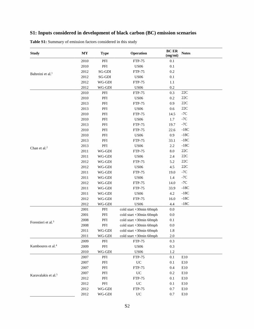
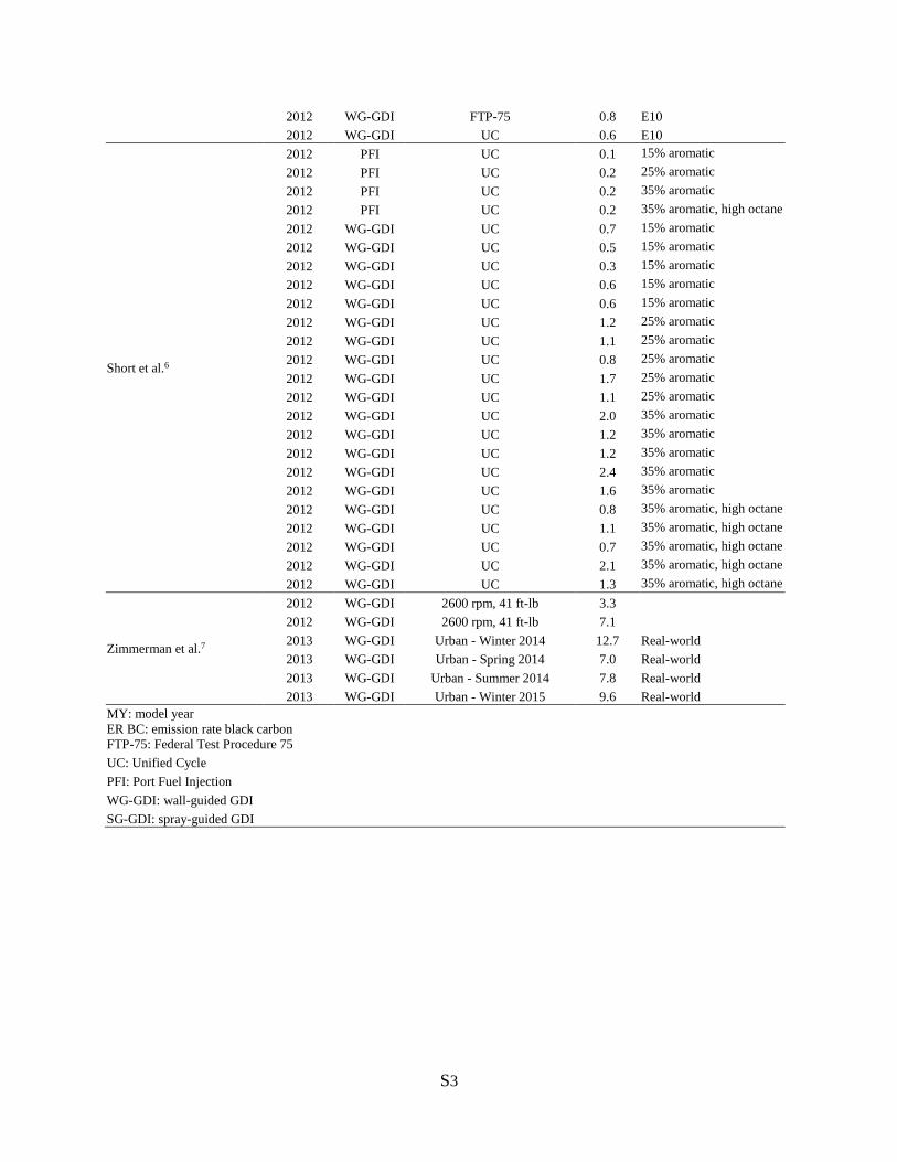
S1: Inputs considered in development of black carbon (BC) emission scenarios

Table S1: Summary of emission factors considered in this study

Study MY Type Operation BC ER

(mg/mi) Notes

Bahreini et al.1

2010 PFI FTP-75 0.1

2010 PFI US06 0.1

2012 SG-GDI FTP-75 0.2

2012 SG-GDI US06 0.1

2012 WG-GDI FTP-75 1.1

2012 WG-GDI US06 0.2

Chan et al.2

2010 PFI FTP-75 0.3 22C

2010 PFI US06 0.2 22C

2013 PFI FTP-75 0.9 22C

2013 PFI US06 0.6 22C

2010 PFI FTP-75 14.5 -7C

2010 PFI US06 1.7 -7C

2013 PFI FTP-75 19.7 -7C

2010 PFI FTP-75 22.6 -18C

2010 PFI US06 0.9 -18C

2013 PFI FTP-75 33.1 -18C

2013 PFI US06 2.2 -18C

2011 WG-GDI FTP-75 8.0 22C

2011 WG-GDI US06 2.4 22C

2012 WG-GDI FTP-75 5.2 22C

2012 WG-GDI US06 4.5 22C

2011 WG-GDI FTP-75 19.0 -7C

2011 WG-GDI US06 1.4 -7C

2012 WG-GDI FTP-75 14.0 -7C

2011 WG-GDI FTP-75 33.9 -18C

2011 WG-GDI US06 4.2 -18C

2012 WG-GDI FTP-75 16.0 -18C

2012 WG-GDI US06 4.4 -18C

Forestieri et al.3

2001 PFI cold start +30min 60mph 0.0




2011 WG-GDI cold start +30min 60mph 1.8

2011 WG-GDI cold start +30min 60mph 2.0

Kamboures et al.4

2009 PFI FTP-75 0.3

2009 PFI US06 0.3

2010 WG-GDI US06 1.2

Karavalakis et al.5

2007 PFI FTP-75 0.1 E10

2007 PFI UC 0.1 E10

2007 PFI FTP-75 0.4 E10

2007 PFI UC 0.2 E10

2012 PFI FTP-75 0.1 E10

2012 PFI UC 0.1 E10

2012 WG-GDI FTP-75 0.7 E10

2012 WG-GDI UC 0.7 E10

S3

2012 WG-GDI FTP-75 0.8 E10

2012 WG-GDI UC 0.6 E10

Short et al.6

2012 PFI UC 0.1 15% aromatic



2012 PFI UC 0.2 35% aromatic, high octane

2012 WG-GDI UC 0.7 15% aromatic















2012 WG-GDI UC 0.8 35% aromatic, high octane





Zimmerman et al.7

2012 WG-GDI 2600 rpm, 41 ft-lb 3.3

2012 WG-GDI 2600 rpm, 41 ft-lb 7.1

2013 WG-GDI Urban - Winter 2014 12.7 Real-world

2013 WG-GDI Urban - Spring 2014 7.0 Real-world

2013 WG-GDI Urban - Summer 2014 7.8 Real-world

2013 WG-GDI Urban - Winter 2015 9.6 Real-world

MY: model year

ER BC: emission rate black carbon

FTP-75: Federal Test Procedure 75

UC: Unified Cycle

PFI: Port Fuel Injection

WG-GDI: wall-guided GDI

SG-GDI: spray-guided GDI

S4

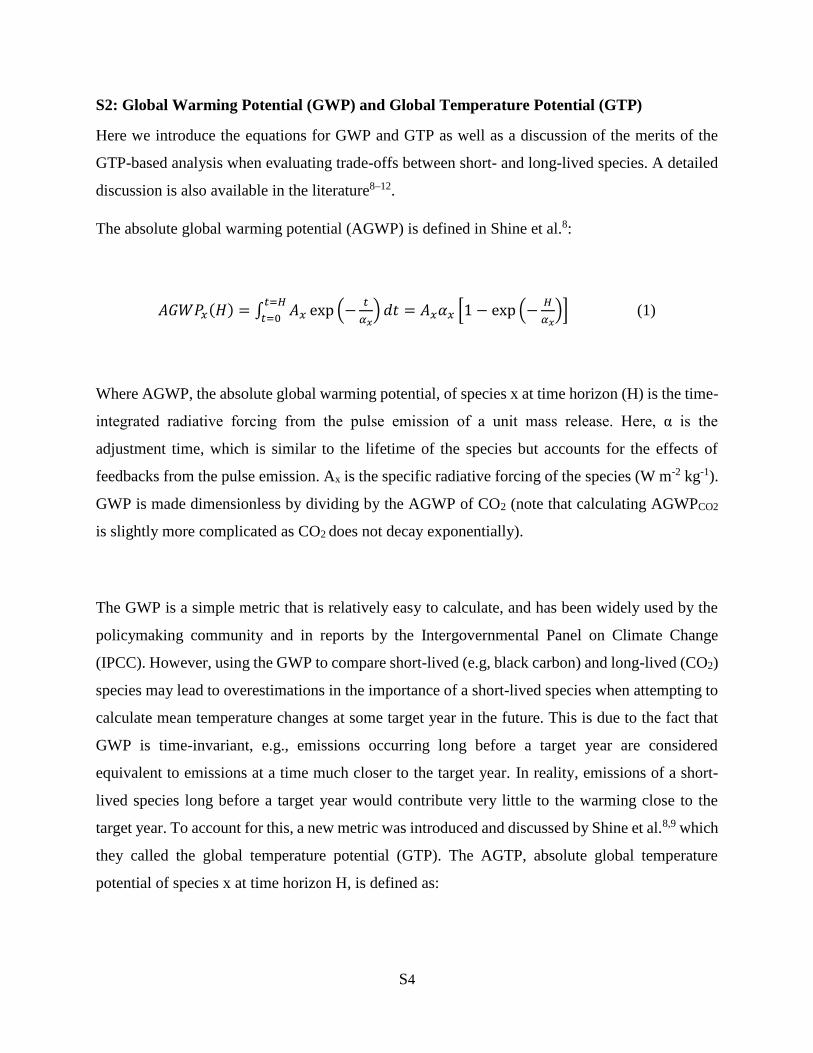
S2: Global Warming Potential (GWP) and Global Temperature Potential (GTP)

Here we introduce the equations for GWP and GTP as well as a discussion of the merits of the

GTP-based analysis when evaluating trade-offs between short- and long-lived species. A detailed

discussion is also available in the literature8–12.

The absolute global warming potential (AGWP) is defined in Shine et al.8:

𝐴𝐺𝑊𝑃𝑥(𝐻) = ∫ 𝐴𝑥 exp (−𝑡

𝛼𝑥) 𝑑𝑡 = 𝐴𝑥𝛼𝑥 [1 − exp (−

𝐻

𝛼𝑥)]

𝑡=𝐻

𝑡=0 (1)

Where AGWP, the absolute global warming potential, of species x at time horizon (H) is the time-

integrated radiative forcing from the pulse emission of a unit mass release. Here, α is the

adjustment time, which is similar to the lifetime of the species but accounts for the effects of

feedbacks from the pulse emission. Ax is the specific radiative forcing of the species (W m-2 kg-1).

GWP is made dimensionless by dividing by the AGWP of CO2 (note that calculating AGWPCO2

is slightly more complicated as CO2 does not decay exponentially).

The GWP is a simple metric that is relatively easy to calculate, and has been widely used by the

policymaking community and in reports by the Intergovernmental Panel on Climate Change

(IPCC). However, using the GWP to compare short-lived (e.g, black carbon) and long-lived (CO2)

species may lead to overestimations in the importance of a short-lived species when attempting to

calculate mean temperature changes at some target year in the future. This is due to the fact that

GWP is time-invariant, e.g., emissions occurring long before a target year are considered

equivalent to emissions at a time much closer to the target year. In reality, emissions of a short-

lived species long before a target year would contribute very little to the warming close to the

target year. To account for this, a new metric was introduced and discussed by Shine et al.8,9 which

they called the global temperature potential (GTP). The AGTP, absolute global temperature

potential of species x at time horizon H, is defined as:

S5

𝐴𝐺𝑇𝑃𝑥(𝐻) =𝐴𝑥

𝐶(𝜏−1−𝛼𝑥−1)

[exp (−𝐻

𝛼𝑥) − exp (−

𝐻

𝜏)] (2)

Where Ax and αx are as defined previously in the GWP, C is the heat capacity of the climate system

and τ is the time-scale of the climate response. Parameters C and τ are needed due to the inclusion

of a simple climate model within the metric (τ=C, where is a climate sensitivity parameter, see

Shine et al.8 for a detailed discussion). As with the GWP, the GTP is made dimensionless by

dividing by the AGTP of CO2 (note that calculating AGTPCO2 is also computed slightly

differently). Comparing equations (1) and (2), equation (2) is an end-point metric whereas equation

(1) is integrative. This metric is a function of both the time horizon and proximity to the target

time horizon, making it more relevant for comparisons of short and long-lived species.

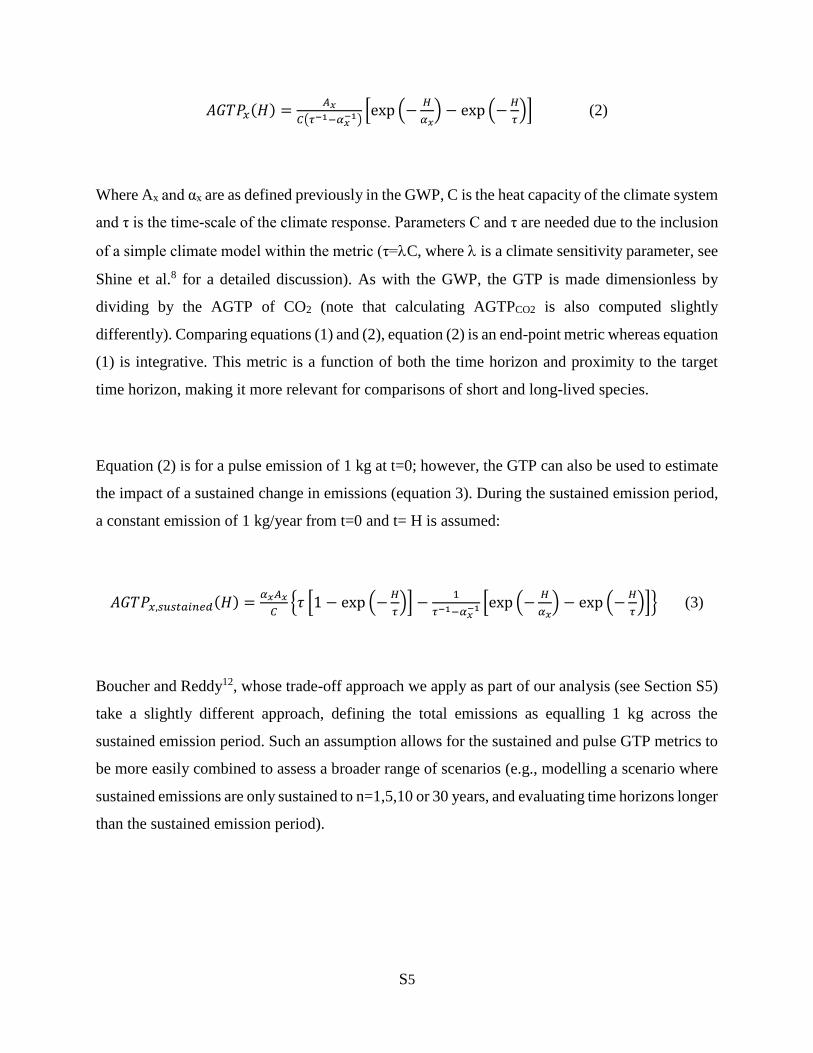
Equation (2) is for a pulse emission of 1 kg at t=0; however, the GTP can also be used to estimate

the impact of a sustained change in emissions (equation 3). During the sustained emission period,

a constant emission of 1 kg/year from t=0 and t= H is assumed:

𝐴𝐺𝑇𝑃𝑥,𝑠𝑢𝑠𝑡𝑎𝑖𝑛𝑒𝑑(𝐻) =𝛼𝑥𝐴𝑥

𝐶{𝜏 [1 − exp (−

𝐻

𝜏)] −

1

𝜏−1−𝛼𝑥−1 [exp (−

𝐻

𝛼𝑥) − exp (−

𝐻

𝜏)]} (3)

Boucher and Reddy12, whose trade-off approach we apply as part of our analysis (see Section S5)

take a slightly different approach, defining the total emissions as equalling 1 kg across the

sustained emission period. Such an assumption allows for the sustained and pulse GTP metrics to

be more easily combined to assess a broader range of scenarios (e.g., modelling a scenario where

sustained emissions are only sustained to n=1,5,10 or 30 years, and evaluating time horizons longer

than the sustained emission period).

S6

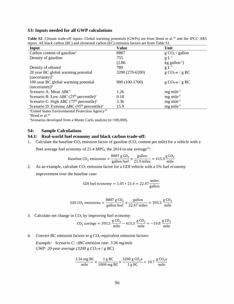
S3: Inputs needed for all GWP calculations

Table S2: Climate trade-off inputs. Global warming potentials (GWPs) are from Bond et al.10 and the IPCC AR5

report. All black carbon (BC) and elemental carbon (EC) emission factors are from Table S1.

Input Value Unit

Carbon content of gasolinea 8887 g CO2 / gallon

Density of gasoline 755 g L-1

(2.86 kg gallon-1)

Density of ethanol 789 g L-1

20 year BC global warming potential

(uncertainty)b

3200 (270-6200) g CO2-e / g BC

100 year BC global warming potential

(uncertainty)b

900 (100-1700) g CO2-e / g BC

Scenario A: Mean ΔBCc 1.26 mg mile-1

Scenario B: Low ΔBC (25th percentile)c 0.18 mg mile-1

Scenario C: High ΔBC (75th percentile)c 3.36 mg mile-1

Scenario D: Extreme ΔBC (95th percentile)c 15.9 mg mile-1 aUnited States Environmental Protection Agency13 bBond et al.10 cScenarios developed from a Monte Carlo analysis (n=100,000).

S4: Sample Calculations

S4.1: Real-world fuel economy and black carbon trade-off:

1. Calculate the baseline CO2 emission factor of gasoline (CO2 content per mile) for a vehicle with a

fleet average fuel economy of 21.4 MPG, the 2014 in-use average14:

Baseline CO2 emissions =8887 g CO2

gallon fuel×

gallon

21.4 miles= 415.3

g CO2

mile

2. As an example, calculate CO2 emission factor for a GDI vehicle with a 5% fuel economy

improvement over the baseline case:

GDI fuel economy = 1.05 ∗ 21.4 = 22.47miles

gallon

GDI CO2 emissions =8887 g CO2

gallon fuel×

gallon

22.47 miles= 395.5

g CO2

mile

3. Calculate net change in CO2 by improving fuel economy:

CO2 savings = 395.5 g CO2

mile− 415.3

g CO2

mile= −19.8

g CO2

mile

4. Convert BC emission factors to g CO2-equivalent emission factors:

Example: Scenario C: ΔBC emission rate: 3.36 mg/mile

GWP: 20-year average (3200 g CO2-e / g BC)

3.36 mg BC

mile×

1 g BC

1000 mg BC×

3200 g CO2e

1 g BC= 10.7

g CO2e

mile

S7

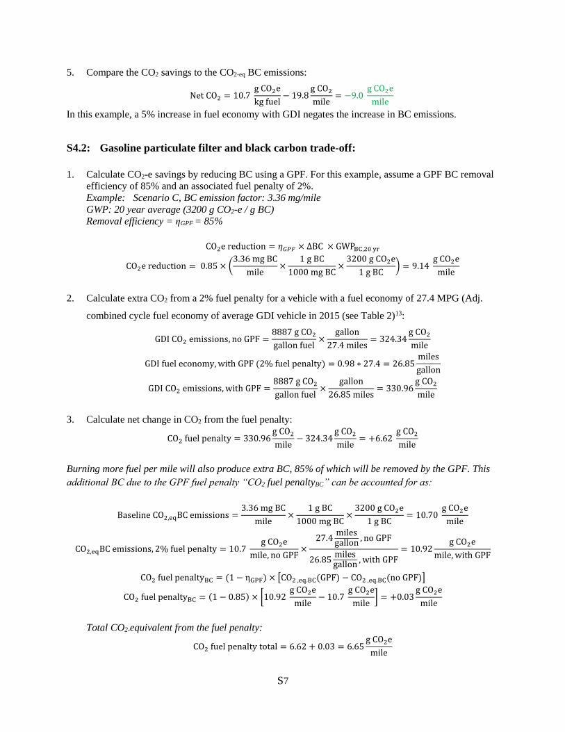
5. Compare the CO2 savings to the CO2-eq BC emissions:

Net CO2 = 10.7 g CO2e

kg fuel− 19.8

g CO2

mile= −9.0

g CO2e

mile

In this example, a 5% increase in fuel economy with GDI negates the increase in BC emissions.

S4.2: Gasoline particulate filter and black carbon trade-off:

1. Calculate CO2-e savings by reducing BC using a GPF. For this example, assume a GPF BC removal

efficiency of 85% and an associated fuel penalty of 2%.

Example: Scenario C, BC emission factor: 3.36 mg/mile

GWP: 20 year average (3200 g CO2-e / g BC)

Removal efficiency = ηGPF = 85%

CO2e reduction = 𝜂𝐺𝑃𝐹 × ∆BC × GWPBC,20 yr

CO2e reduction = 0.85 × (3.36 mg BC

mile×

1 g BC

1000 mg BC×

3200 g CO2e

1 g BC) = 9.14

g CO2e

mile

2. Calculate extra CO2 from a 2% fuel penalty for a vehicle with a fuel economy of 27.4 MPG (Adj.

combined cycle fuel economy of average GDI vehicle in 2015 (see Table 2)13:

GDI CO2 emissions, no GPF =8887 g CO2

gallon fuel×

gallon

27.4 miles= 324.34

g CO2

mile

GDI fuel economy, with GPF (2% fuel penalty) = 0.98 ∗ 27.4 = 26.85miles

gallon

GDI CO2 emissions, with GPF =8887 g CO2

gallon fuel×

gallon

26.85 miles= 330.96

g CO2

mile

3. Calculate net change in CO2 from the fuel penalty:

CO2 fuel penalty = 330.96g CO2

mile− 324.34

g CO2

mile= +6.62

g CO2

mile

Burning more fuel per mile will also produce extra BC, 85% of which will be removed by the GPF. This

additional BC due to the GPF fuel penalty “CO2 fuel penaltyBC” can be accounted for as:

Baseline CO2,eqBC emissions =3.36 mg BC

mile×

1 g BC

1000 mg BC×

3200 g CO2e

1 g BC= 10.70

g CO2e

mile

CO2,eqBC emissions, 2% fuel penalty = 10.7 g CO2e

mile, no GPF×

27.4milesgallon

, no GPF

26.85milesgallon

, with GPF= 10.92

g CO2e

mile, with GPF

CO2 fuel penaltyBC = (1 − ηGPF) × [CO2 ,eq.BC(GPF) − CO2 ,eq.BC(no GPF)]

CO2 fuel penaltyBC = (1 − 0.85) × [10.92 g CO2e

mile− 10.7

g CO2e

mile] = +0.03

g CO2e

mile

Total CO2-equivalent from the fuel penalty:

CO2 fuel penalty total = 6.62 + 0.03 = 6.65g CO2e

mile

S8

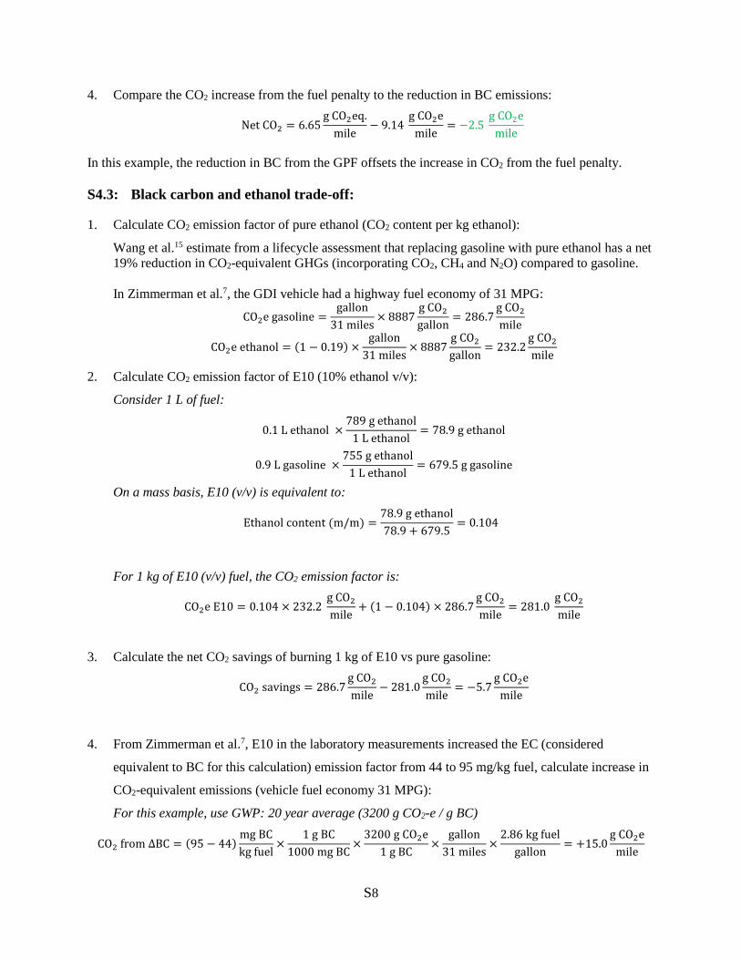
4. Compare the CO2 increase from the fuel penalty to the reduction in BC emissions:

Net CO2 = 6.65g CO2eq.

mile− 9.14

g CO2e

mile= −2.5

g CO2e

mile

In this example, the reduction in BC from the GPF offsets the increase in CO2 from the fuel penalty.

S4.3: Black carbon and ethanol trade-off:

1. Calculate CO2 emission factor of pure ethanol (CO2 content per kg ethanol):

Wang et al.15 estimate from a lifecycle assessment that replacing gasoline with pure ethanol has a net

19% reduction in CO2-equivalent GHGs (incorporating CO2, CH4 and N2O) compared to gasoline.

In Zimmerman et al.7, the GDI vehicle had a highway fuel economy of 31 MPG:

CO2e gasoline =gallon

31 miles× 8887

g CO2

gallon= 286.7

g CO2

mile

CO2e ethanol = (1 − 0.19) ×gallon

31 miles× 8887

g CO2

gallon= 232.2

g CO2

mile

2. Calculate CO2 emission factor of E10 (10% ethanol v/v):

Consider 1 L of fuel:

0.1 L ethanol ×789 g ethanol

1 L ethanol= 78.9 g ethanol

0.9 L gasoline ×755 g ethanol

1 L ethanol= 679.5 g gasoline

On a mass basis, E10 (v/v) is equivalent to:

Ethanol content (m/m) =78.9 g ethanol

78.9 + 679.5= 0.104

For 1 kg of E10 (v/v) fuel, the CO2 emission factor is:

CO2e E10 = 0.104 × 232.2 g CO2

mile+ (1 − 0.104) × 286.7

g CO2

mile= 281.0

g CO2

mile

3. Calculate the net CO2 savings of burning 1 kg of E10 vs pure gasoline:

CO2 savings = 286.7g CO2

mile− 281.0

g CO2

mile= −5.7

g CO2e

mile

4. From Zimmerman et al.7, E10 in the laboratory measurements increased the EC (considered

equivalent to BC for this calculation) emission factor from 44 to 95 mg/kg fuel, calculate increase in

CO2-equivalent emissions (vehicle fuel economy 31 MPG):

For this example, use GWP: 20 year average (3200 g CO2-e / g BC)

CO2 from ∆BC = (95 − 44)mg BC

kg fuel×

1 g BC

1000 mg BC×

3200 g CO2e

1 g BC×

gallon

31 miles×

2.86 kg fuel

gallon= +15.0

g CO2e

mile

S9

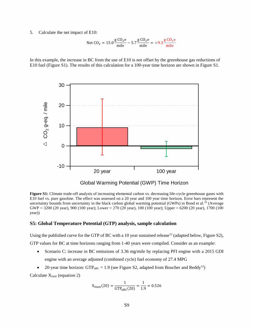
5. Calculate the net impact of E10:

Net CO2 = 15.0g CO2e

mile− 5.7

g CO2e

mile= +9.3

g CO2e

mile

In this example, the increase in BC from the use of E10 is not offset by the greenhouse gas reductions of

E10 fuel (Figure S1). The results of this calculation for a 100-year time horizon are shown in Figure S1.

Figure S1: Climate trade-off analysis of increasing elemental carbon vs. decreasing life-cycle greenhouse gases with

E10 fuel vs. pure gasoline. The effect was assessed on a 20 year and 100 year time horizon. Error bars represent the

uncertainty bounds from uncertainty in the black carbon global warming potential (GWPs) in Bond et al.10 (Average

GWP = 3200 (20 year), 900 (100 year); Lower = 270 (20 year), 100 (100 year); Upper = 6200 (20 year), 1700 (100

year))

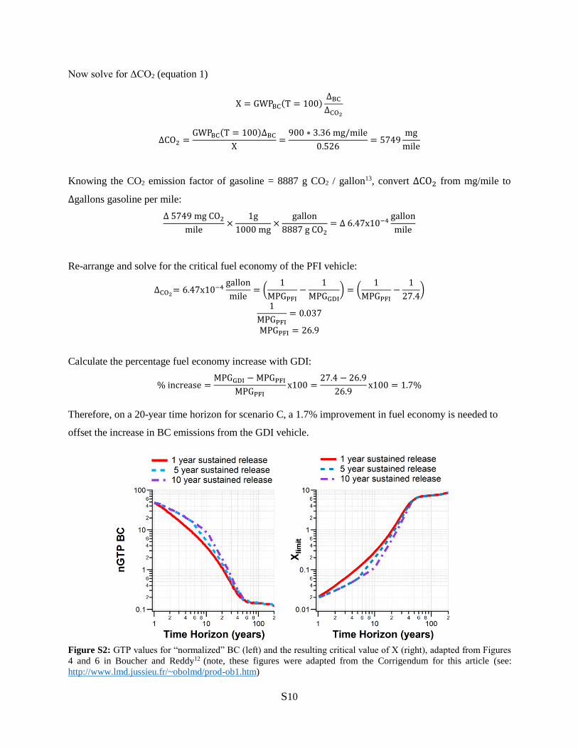
S5: Global Temperature Potential (GTP) analysis, sample calculation

Using the published curve for the GTP of BC with a 10 year sustained release12 (adapted below, Figure S2),

GTP values for BC at time horizons ranging from 1-40 years were compiled. Consider as an example:

Scenario C: increase in BC emissions of 3.36 mg/mile by replacing PFI engine with a 2015 GDI

engine with an average adjusted (combined cycle) fuel economy of 27.4 MPG

20-year time horizon: GTPnBC = 1.9 (see Figure S2, adapted from Boucher and Reddy12)

Calculate Xlimit (equation 2)

Xlimit(20) =1

GTPnBC(20)=

1

1.9= 0.526

30

20

10

0

-10

CO

2 g

-eq

. /

mile

20 year 100 year

Global Warming Potential (GWP) Time Horizon

S10

Now solve for ΔCO2 (equation 1)

X = GWPBC(T = 100)∆BC

∆CO2

∆CO2 =GWPBC(T = 100)∆BC

X=

900 ∗ 3.36 mg/mile

0.526= 5749

mg

mile

Knowing the CO2 emission factor of gasoline = 8887 g CO2 / gallon13, convert ∆CO2 from mg/mile to

∆gallons gasoline per mile:

∆ 5749 mg CO2

mile×

1g

1000 mg×

gallon

8887 g CO2

= ∆ 6.47x10−4gallon

mile

Re-arrange and solve for the critical fuel economy of the PFI vehicle:

∆CO2= 6.47x10−4

gallon

mile= (

1

MPGPFI

−1

MPGGDI

) = (1

MPGPFI

−1

27.4)

1

MPGPFI

= 0.037

MPGPFI = 26.9

Calculate the percentage fuel economy increase with GDI:

% increase =MPGGDI − MPGPFI

MPGPFI

x100 =27.4 − 26.9

26.9x100 = 1.7%

Therefore, on a 20-year time horizon for scenario C, a 1.7% improvement in fuel economy is needed to

offset the increase in BC emissions from the GDI vehicle.

Figure S2: GTP values for “normalized” BC (left) and the resulting critical value of X (right), adapted from Figures

4 and 6 in Boucher and Reddy12 (note, these figures were adapted from the Corrigendum for this article (see:

http://www.lmd.jussieu.fr/~obolmd/prod-ob1.htm)

http://www.lmd.jussieu.fr/~obolmd/prod-ob1.htm

S11

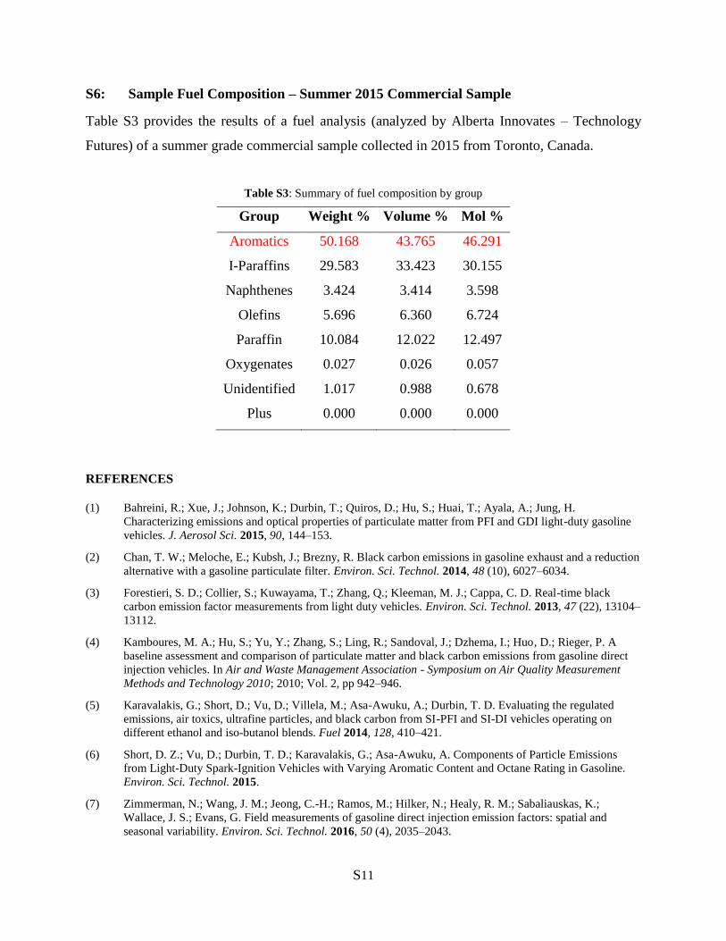
S6: Sample Fuel Composition – Summer 2015 Commercial Sample

Table S3 provides the results of a fuel analysis (analyzed by Alberta Innovates – Technology

Futures) of a summer grade commercial sample collected in 2015 from Toronto, Canada.

Table S3: Summary of fuel composition by group

Group Weight % Volume % Mol %

Aromatics 50.168 43.765 46.291

I-Paraffins 29.583 33.423 30.155

Naphthenes 3.424 3.414 3.598

Olefins 5.696 6.360 6.724

Paraffin 10.084 12.022 12.497

Oxygenates 0.027 0.026 0.057

Unidentified 1.017 0.988 0.678

Plus 0.000 0.000 0.000

REFERENCES

(1) Bahreini, R.; Xue, J.; Johnson, K.; Durbin, T.; Quiros, D.; Hu, S.; Huai, T.; Ayala, A.; Jung, H.

Characterizing emissions and optical properties of particulate matter from PFI and GDI light-duty gasoline

vehicles. J. Aerosol Sci. 2015, 90, 144–153.

(2) Chan, T. W.; Meloche, E.; Kubsh, J.; Brezny, R. Black carbon emissions in gasoline exhaust and a reduction

alternative with a gasoline particulate filter. Environ. Sci. Technol. 2014, 48 (10), 6027–6034.

(3) Forestieri, S. D.; Collier, S.; Kuwayama, T.; Zhang, Q.; Kleeman, M. J.; Cappa, C. D. Real-time black

carbon emission factor measurements from light duty vehicles. Environ. Sci. Technol. 2013, 47 (22), 13104–

13112.

(4) Kamboures, M. A.; Hu, S.; Yu, Y.; Zhang, S.; Ling, R.; Sandoval, J.; Dzhema, I.; Huo, D.; Rieger, P. A

baseline assessment and comparison of particulate matter and black carbon emissions from gasoline direct

injection vehicles. In Air and Waste Management Association - Symposium on Air Quality Measurement

Methods and Technology 2010; 2010; Vol. 2, pp 942–946.

(5) Karavalakis, G.; Short, D.; Vu, D.; Villela, M.; Asa-Awuku, A.; Durbin, T. D. Evaluating the regulated

emissions, air toxics, ultrafine particles, and black carbon from SI-PFI and SI-DI vehicles operating on

different ethanol and iso-butanol blends. Fuel 2014, 128, 410–421.

(6) Short, D. Z.; Vu, D.; Durbin, T. D.; Karavalakis, G.; Asa-Awuku, A. Components of Particle Emissions

from Light-Duty Spark-Ignition Vehicles with Varying Aromatic Content and Octane Rating in Gasoline.

Environ. Sci. Technol. 2015.

(7) Zimmerman, N.; Wang, J. M.; Jeong, C.-H.; Ramos, M.; Hilker, N.; Healy, R. M.; Sabaliauskas, K.;

Wallace, J. S.; Evans, G. Field measurements of gasoline direct injection emission factors: spatial and

seasonal variability. Environ. Sci. Technol. 2016, 50 (4), 2035–2043.

S12

(8) Shine, K. P.; Fuglestvedt, J. S.; Hailemariam, K.; Stuber, N. Alternatives to the Global Warming Potential

for Comparing Climate Impacts of Emissions of Greenhouse Gases. Clim. Change 2005, 68, 281–302.

(9) Shine, K. P.; Berntsen, T. K.; Fuglestvedt, J. S.; Bieltvedt Skeie, R.; Stuber, N. Comparing the climate effect

of emissions of short- and long-lived climate agents. Philos. Trans. R. Soc. A 2007, 265, 1903–1914.

(10) Bond, T. C.; Doherty, S. J.; Fahey, D. W.; Forster, P. M.; Berntsen, T.; DeAngelo, B. J.; Flanner, M. G.;

Ghan, S.; Kärcher, B.; Koch, D.; et al. Bounding the role of black carbon in the climate system: A scientific

assessment. J. Geophys. Res. Atmos. 2013, 118 (11), 5380–5552.

(11) Stohl, A.; Aamaas, B.; Amann, M.; Baker, L. H.; Bellouin, N.; Berntsen, T. K.; Boucher, O.; Cherian, R.;

Collins, W.; Daskalakis, N.; et al. Evaluating the climate and air quality impacts of short-lived pollutants.

Atmos. Chem. Phys. Discuss. 2015, 15 (11), 15155–15241.

(12) Boucher, O.; Reddy, M. S. Climate trade-off between black carbon and carbon dioxide emissions. Energy

Policy 2008, 36 (1), 193–200.

(13) United States Environmental Protection Agency. Light-Duty Automotive Technology, Carbon Dioxide

Emissions, and Fuel Economy Trends: 1975 Through 2015; 2015.

(14) United States Department of Transportation. Table 4-23: Average Fuel Efficiency of U.S. Light Duty

Vehicles | Bureau of Transportation Statistics

http://www.rita.dot.gov/bts/sites/rita.dot.gov.bts/files/publications/national_transportation_statistics/html/tab

le_04_23.html.

(15) Wang, M.; Wu, M.; Huo, H. Life-cycle energy and greenhouse gas emission impacts of different corn

ethanol plant types. Environ. Res. Lett. 2007, 2 (2), 024001.

assessing the climate trade-offs of gasoline direct ...€¦ · assessing the climate trade-offs of...

Documents