assembly language programming: arm cortex-m3 - … language...μcontroller constructed around an arm...
TRANSCRIPT


Assembly Language Programming

Assembly LanguageProgramming
ARM Cortex-M3
Vincent Mahout
First published 2012 in Great Britain and the United States by ISTE Ltd and John Wiley & Sons, Inc.
Apart from any fair dealing for the purposes of research or private study, or criticism or review, aspermitted under the Copyright, Designs and Patents Act 1988, this publication may only be reproduced,stored or transmitted, in any form or by any means, with the prior permission in writing of the publishers,or in the case of reprographic reproduction in accordance with the terms and licenses issued by theCLA. Enquiries concerning reproduction outside these terms should be sent to the publishers at theundermentioned address:
ISTE Ltd John Wiley & Sons, Inc.27-37 St George’s Road 111 River StreetLondon SW19 4EU Hoboken, NJ 07030UK USA
www.iste.co.uk www.wiley.com
© ISTE Ltd 2012
The rights of Vincent Mahout to be identified as the author of this work have been asserted by him inaccordance with the Copyright, Designs and Patents Act 1988.____________________________________________________________________________________
Library of Congress Cataloging-in-Publication Data
Mahout, Vincent.Assembly language programming : ARM Cortex-M3 / Vincent Mahout.p. cm.Includes bibliographical references and index.ISBN 978-1-84821-329-61. Embedded computer systems. 2. Microprocessors. 3. Assembler language (Computer programlanguage) I. Title.TK7895.E42M34 2012005.2--dc23
2011049418
British Library Cataloguing-in-Publication DataA CIP record for this book is available from the British LibraryISBN: 978-1-84821-329-6
Printed and bound in Great Britain by CPI Group (UK) Ltd., Croydon, Surrey CR0 4YY
Table of Contents
Preface . . . . . . . . . . . . . . . . . . . . . . . . . . . . . . . . . . . . . . . . . . . ix
Chapter 1. Overview of Cortex-M3 Architecture . . . . . . . . . . . . . . . . 1
1.1. Assembly language versus the assembler . . . . . . . . . . . . . . . . . . 11.2. The world of ARM . . . . . . . . . . . . . . . . . . . . . . . . . . . . . . . 21.2.1. Cortex-M3 . . . . . . . . . . . . . . . . . . . . . . . . . . . . . . . . . . 31.2.2. The Cortex-M3 core in STM32. . . . . . . . . . . . . . . . . . . . . . 7
Chapter 2. The Core of Cortex-M3 . . . . . . . . . . . . . . . . . . . . . . . . . 15
2.1. Modes, privileges and states . . . . . . . . . . . . . . . . . . . . . . . . . . 152.2. Registers . . . . . . . . . . . . . . . . . . . . . . . . . . . . . . . . . . . . . 172.2.1. Registers R0 to R12 . . . . . . . . . . . . . . . . . . . . . . . . . . . . 192.2.2. The R13 register, also known as SP . . . . . . . . . . . . . . . . . . . 192.2.3. The R14 register, also known as LR. . . . . . . . . . . . . . . . . . . 202.2.4. The R15 or PC register. . . . . . . . . . . . . . . . . . . . . . . . . . . 212.2.5. The xPSR register . . . . . . . . . . . . . . . . . . . . . . . . . . . . . 22
Chapter 3. The Proper Use of Assembly Directives . . . . . . . . . . . . . . . 25
3.1. The concept of the directive . . . . . . . . . . . . . . . . . . . . . . . . . . 253.1.1. Typographic conventions and use of symbols . . . . . . . . . . . . . 26
3.2. Structure of a program . . . . . . . . . . . . . . . . . . . . . . . . . . . . . 273.2.1. The AREA sections . . . . . . . . . . . . . . . . . . . . . . . . . . . . 28
3.3. A section of code . . . . . . . . . . . . . . . . . . . . . . . . . . . . . . . . 293.3.1. Labels. . . . . . . . . . . . . . . . . . . . . . . . . . . . . . . . . . . . . 293.3.2. Mnemonic . . . . . . . . . . . . . . . . . . . . . . . . . . . . . . . . . . 313.3.3. Operands . . . . . . . . . . . . . . . . . . . . . . . . . . . . . . . . . . . 323.3.4. Comments . . . . . . . . . . . . . . . . . . . . . . . . . . . . . . . . . . 343.3.5. Procedure. . . . . . . . . . . . . . . . . . . . . . . . . . . . . . . . . . . 35
vi Assembly Language Programming
3.4. The data section . . . . . . . . . . . . . . . . . . . . . . . . . . . . . . . . . 363.4.1. Simple reservation . . . . . . . . . . . . . . . . . . . . . . . . . . . . . 363.4.2. Reservation with initialization . . . . . . . . . . . . . . . . . . . . . . 373.4.3. Data initialization: the devil is in the details . . . . . . . . . . . . . . 39
3.5. Is that all? . . . . . . . . . . . . . . . . . . . . . . . . . . . . . . . . . . . . . 393.5.1. Memory management directives . . . . . . . . . . . . . . . . . . . . . 403.5.2. Project management directives . . . . . . . . . . . . . . . . . . . . . . 413.5.3. Various and varied directives . . . . . . . . . . . . . . . . . . . . . . . 44
Chapter 4. Operands of Instructions . . . . . . . . . . . . . . . . . . . . . . . . 47
4.1. The constant and renaming. . . . . . . . . . . . . . . . . . . . . . . . . . . 484.2. Operands for common instructions . . . . . . . . . . . . . . . . . . . . . . 494.2.1. Use of registers . . . . . . . . . . . . . . . . . . . . . . . . . . . . . . . 494.2.2. The immediate operand . . . . . . . . . . . . . . . . . . . . . . . . . . 53
4.3. Memory access operands: addressing modes . . . . . . . . . . . . . . . . 574.3.1. The pointer concept . . . . . . . . . . . . . . . . . . . . . . . . . . . . 584.3.2. Addressing modes . . . . . . . . . . . . . . . . . . . . . . . . . . . . . 59
Chapter 5. Instruction Set . . . . . . . . . . . . . . . . . . . . . . . . . . . . . . . 63
5.1. Reading guide . . . . . . . . . . . . . . . . . . . . . . . . . . . . . . . . . . 635.1.1. List of possible “condition” suffixes. . . . . . . . . . . . . . . . . . . 65
5.2. Arithmetic instructions . . . . . . . . . . . . . . . . . . . . . . . . . . . . . 665.3. Logical and bit manipulation instructions . . . . . . . . . . . . . . . . . . 705.4. Internal transfer instructions . . . . . . . . . . . . . . . . . . . . . . . . . . 755.5. Test instructions . . . . . . . . . . . . . . . . . . . . . . . . . . . . . . . . . 765.6. Branch instructions . . . . . . . . . . . . . . . . . . . . . . . . . . . . . . . 775.7. Load/store instructions . . . . . . . . . . . . . . . . . . . . . . . . . . . . . 805.7.1. Simple transfers . . . . . . . . . . . . . . . . . . . . . . . . . . . . . . . 805.7.2. Multiple transfers . . . . . . . . . . . . . . . . . . . . . . . . . . . . . . 825.7.3. Access to the system stack . . . . . . . . . . . . . . . . . . . . . . . . 84
5.8. “System” instructions and others . . . . . . . . . . . . . . . . . . . . . . . 85
Chapter 6. Algorithmic and Data Structures . . . . . . . . . . . . . . . . . . . 87
6.1. Flowchart versus algorithm . . . . . . . . . . . . . . . . . . . . . . . . . . 876.2. Alternative structures . . . . . . . . . . . . . . . . . . . . . . . . . . . . . . 896.2.1. Simple (or shortened) alternative. . . . . . . . . . . . . . . . . . . . . 896.2.2. Complete alternative . . . . . . . . . . . . . . . . . . . . . . . . . . . . 906.2.3. Special case of the alternative . . . . . . . . . . . . . . . . . . . . . . 936.2.4. Multiple choice . . . . . . . . . . . . . . . . . . . . . . . . . . . . . . . 94
6.3. Iterative structures . . . . . . . . . . . . . . . . . . . . . . . . . . . . . . . . 986.3.1. The Repeat…Until loop . . . . . . . . . . . . . . . . . . . . . . . . . . 98
Table of Contents vii
6.3.2. TheWhile…Do loop . . . . . . . . . . . . . . . . . . . . . . . . . . . . 1026.3.3. The For… loop . . . . . . . . . . . . . . . . . . . . . . . . . . . . . . . 105
6.4. Compound conditions. . . . . . . . . . . . . . . . . . . . . . . . . . . . . . 1066.4.1. Alternative with AND . . . . . . . . . . . . . . . . . . . . . . . . . . . 1076.4.2. Iteration with AND. . . . . . . . . . . . . . . . . . . . . . . . . . . . . 1086.4.3. Alternative with OR . . . . . . . . . . . . . . . . . . . . . . . . . . . . 1096.4.4. Iteration with OR . . . . . . . . . . . . . . . . . . . . . . . . . . . . . . 110
6.5. Data structure. . . . . . . . . . . . . . . . . . . . . . . . . . . . . . . . . . . 1116.5.1. Table in one dimension . . . . . . . . . . . . . . . . . . . . . . . . . . 1116.5.2. Tables in multiple dimensions . . . . . . . . . . . . . . . . . . . . . . 1126.5.3. Registration . . . . . . . . . . . . . . . . . . . . . . . . . . . . . . . . . 1136.5.4. Non-dimensional table, character string. . . . . . . . . . . . . . . . . 1136.5.5. Queue . . . . . . . . . . . . . . . . . . . . . . . . . . . . . . . . . . . . . 1146.5.6. Stack . . . . . . . . . . . . . . . . . . . . . . . . . . . . . . . . . . . . . 115
Chapter 7. Internal Modularity . . . . . . . . . . . . . . . . . . . . . . . . . . . 119
7.1. Detailing the concept of procedure . . . . . . . . . . . . . . . . . . . . . . 1197.1.1. Simple call . . . . . . . . . . . . . . . . . . . . . . . . . . . . . . . . . . 1197.1.2. Nested calls . . . . . . . . . . . . . . . . . . . . . . . . . . . . . . . . . 1197.1.3. “Red wire” example . . . . . . . . . . . . . . . . . . . . . . . . . . . . 121
7.2. Procedure arguments . . . . . . . . . . . . . . . . . . . . . . . . . . . . . . 1237.2.1. Usefulness of arguments. . . . . . . . . . . . . . . . . . . . . . . . . . 1237.2.2. Arguments by value and by reference . . . . . . . . . . . . . . . . . . 1237.2.3. Passing arguments by general registers . . . . . . . . . . . . . . . . . 1237.2.4. Passing arguments by a stack . . . . . . . . . . . . . . . . . . . . . . . 1267.2.5. Passing arguments by the system stack . . . . . . . . . . . . . . . . . 1337.2.6. On the art of mixing . . . . . . . . . . . . . . . . . . . . . . . . . . . . 136
7.3. Local data . . . . . . . . . . . . . . . . . . . . . . . . . . . . . . . . . . . . . 1367.3.1. Simple reservation of local data . . . . . . . . . . . . . . . . . . . . . 1377.3.2. Using a chained list. . . . . . . . . . . . . . . . . . . . . . . . . . . . . 143
Chapter 8. Managing Exceptions. . . . . . . . . . . . . . . . . . . . . . . . . . . 147
8.1. What happens during Reset?. . . . . . . . . . . . . . . . . . . . . . . . . . 1488.2. Possible exceptions . . . . . . . . . . . . . . . . . . . . . . . . . . . . . . . 1518.2.1. Traps . . . . . . . . . . . . . . . . . . . . . . . . . . . . . . . . . . . . . 1538.2.2. Interrupts . . . . . . . . . . . . . . . . . . . . . . . . . . . . . . . . . . . 159
8.3. Priority management . . . . . . . . . . . . . . . . . . . . . . . . . . . . . . 1618.3.1. Priority levels and sublevels . . . . . . . . . . . . . . . . . . . . . . . 1628.3.2. The nested mechanism. . . . . . . . . . . . . . . . . . . . . . . . . . . 166
8.4. Entry and return in exception processing . . . . . . . . . . . . . . . . . . 1678.4.1. Re-routing . . . . . . . . . . . . . . . . . . . . . . . . . . . . . . . . . . 1678.4.2. Return. . . . . . . . . . . . . . . . . . . . . . . . . . . . . . . . . . . . . 169
viii Assembly Language Programming
8.4.3. “Tail-chaining” and “Late-arriving” . . . . . . . . . . . . . . . . . . . 1698.4.4. Other useful registers for the NVIC . . . . . . . . . . . . . . . . . . . 170
Chapter 9. From Listing to Executable: External Modularity . . . . . . . . 173
9.1. External modularity . . . . . . . . . . . . . . . . . . . . . . . . . . . . . . . 1759.1.1. Generic example . . . . . . . . . . . . . . . . . . . . . . . . . . . . . . 1759.1.2. Assembly by pieces . . . . . . . . . . . . . . . . . . . . . . . . . . . . 1789.1.3. Advantages of assembly by pieces. . . . . . . . . . . . . . . . . . . . 1789.1.4. External symbols . . . . . . . . . . . . . . . . . . . . . . . . . . . . . . 1799.1.5. IMPORT and EXPORT directives . . . . . . . . . . . . . . . . . . . . 181
9.2. The role of the assembler. . . . . . . . . . . . . . . . . . . . . . . . . . . . 1829.2.1. Files produced by the assembler . . . . . . . . . . . . . . . . . . . . . 1839.2.2. Placement counters . . . . . . . . . . . . . . . . . . . . . . . . . . . . . 1859.2.3. First pass: symbol table . . . . . . . . . . . . . . . . . . . . . . . . . . 1859.2.4. Second pass: translation . . . . . . . . . . . . . . . . . . . . . . . . . . 1869.2.5. Relocation table . . . . . . . . . . . . . . . . . . . . . . . . . . . . . . . 187
9.3. The role of the linker . . . . . . . . . . . . . . . . . . . . . . . . . . . . . . 1889.3.1. Functioning principle . . . . . . . . . . . . . . . . . . . . . . . . . . . 1889.3.2. The products of the linker . . . . . . . . . . . . . . . . . . . . . . . . . 190
9.4. The loader and the debugging unit . . . . . . . . . . . . . . . . . . . . . . 196
Appendices . . . . . . . . . . . . . . . . . . . . . . . . . . . . . . . . . . . . . . . . 199
Appendix A. Instruction Set – Alphabetical List . . . . . . . . . . . . . . . . . 201
Appendix B. The SysTick Timer . . . . . . . . . . . . . . . . . . . . . . . . . . . 209
Appendix C. Example of a “Bootstrap” File. . . . . . . . . . . . . . . . . . . . 217
Appendix D. The GNU Assembler . . . . . . . . . . . . . . . . . . . . . . . . . . 227
Bibliography . . . . . . . . . . . . . . . . . . . . . . . . . . . . . . . . . . . . . . . 239
Index . . . . . . . . . . . . . . . . . . . . . . . . . . . . . . . . . . . . . . . . . . . . 241
Preface
To be able to plan and write this type of book, you need a good workenvironment. In my case, I was able to benefit from the best working conditions forthis enterprise. In terms of infrastructure and material, the Institut National deSciences Appliquées de Toulouse, France (Toulouse National Institute of AppliedSciences), and in particular their Electrical and Computer Engineering Department,has never hesitated to invest in computer systems engineering, so that the training ofour future engineers will always be able to keep up with rapid technological change.I express my profound gratitude to this institution. These systems would not haveamounted to much unless, over the years, there was an educational and technicalteam bringing their enthusiasm and dynamism to implement them. The followingpages also contain the hard work of Pascal Acco, Guillaume Auriol, Pierre-Emmanuel Hladik, Didier Le Botlan, José Martin, Sébastien Di Mercurio andThierry Rocacher. I thank them sincerely. Two final respectful and friendly nods goto François Pompignac and Bernard Fauré who, before retirement, did much work tofertilize this now thriving land.
When writing a book on the assembly language of a μprocessor, we know inadvance that it will not register in posterity. By its very nature, an assemblylanguage has the same life expectancy as the processor it supports – perhaps 20years at best. What’s more, this type of programming is obviously not used for thedevelopment of software projects and so is of little consequence.
Assembly language programming is, however, an indispensable step inunderstanding the internal functioning of a μprocessor. This is why it is still widelytaught in industrial computer training, and particularly in training engineers. It isclear that a good theoretical knowledge of a particular assembly language, combinedwith a practical training phase, allows for easier learning of other programminglanguages, whether they are the assembly languages of other processors orhigh-level languages.
x Assembly Language Programming
Thus, this book intends to dissect programming in the assembly language of aμcontroller constructed around an ARM Cortex-M3 core. The choice of thisμcontroller rests on the desire to explain:
– a 32-bit processor: the choice of the ARM designer is essential in the 32-bitworld. This type of processor occupies, for example, 95% of the market in thedomain of mobile telephony;
– a processor of recent conception and architecture: the first licenses forCortex-M3 are dated October 2004 and those for STMicroelectronics’ 32-bit flashmicrocontrollers (STM32) were given in June 2007;
– a processor adapted to the embedded world, based on the observation that 80%of software development activity involves embedded systems.
This book had been written to be as generic as possible. It is certainly based onthe architecture and instruction set of Cortex-M3, but with the intention ofexplaining the basic mechanisms of assembly language programming. In this waywe can use systematically modular programming to show how basic algorithmicstructures can be programmed in assembly language. This book also presents manyillustrative examples, meaning it is also practical.
Chapter 1
Overview of Cortex-M3 Architecture
A computer program is usually defined as a sequence of instructions that act ondata and return an expected result. In a high-level language, the sequence and dataare described in a symbolic, abstract form. It is necessary to use a compiler totranslate them into machine language instructions, which are only understood by theprocessor. Assembly language is directly derived from machine language, so whenprogramming in assembly language the programmer is forced to see things from thepoint of view of the processor.
1.1. Assembly language versus the assembler
When executing a program, a computer processor obeys a series of numericalorders – instructions – that are read from memory: these instructions are encoded inbinary form. The collection of instructions in memory makes up the code of theprogram being executed. Other areas of memory are also used by the processorduring the execution of code: an area containing the data (variables, constants) andan area containing the system stack, which is used by the processor to store, forexample, local data when calling subprograms. Code, data and the system stack arethe three fundamental elements of all programs during their execution.
It is possible to program directly in machine language – that is, to write the bitinstruction sequences in machine language. In practice, however, this is not realistic,even when using a more condensed script thanks to hexadecimal notation(numeration in base 16) for the instructions. It is therefore preferable to use anassembly language. This allows code to be represented by symbolic names, adaptedto human understanding, which correspond to instructions in machine language.
2 Assembly Language Programming
Assembly language also allows the programmer to reserve the space needed for thesystem stack and data areas by giving them an initial value, if necessary. Take thisexample of an instruction to copy in the no. 1 general register of a processor with thevalue 170 (AA in hexadecimal). Here it is, written using the syntax of assemblylanguage studied here:
EXAMPLE 1.1.– A single line of code
MOV R1, #0xAA ; copy (move) value 170 (AA in hexa)
; in register R1
The same instruction, represented in machine language (hexadecimal base), iswritten: E3A010AA. The symbolic name MOV takes the name mnemonic. R1 and#0xAA are the arguments of the instruction. The semicolon indicates the start of acommentary that ends with the current line.
The assembler is a program responsible for translating the program from theassembly language in which it is written into machine language. Upon input, itreceives a source file that is written in assembly language, and creates two files: theobject file containing machine language (and the necessary information for thefabrication of an executable program), and the printout assembly file containing areport that details the work carried out by the assembler.
This book deals with assembly language in general, but focuses on processorsbased on Cortex-M3, as set out by Advanced RISC Machines (abbreviated to ARM).Different designers (Freescale, STmicroelectronics, NXP, etc.) then integrate thisstructure into μcontrollers containing memory and multiple peripherals as well asthis processor core. Part of the documentation regarding this processor core isavailable in PDF format at www.arm.com.
1.2. The world of ARM
ARM does not directly produce semiconductors, but rather provides licenses formicroprocessor cores with 32-bit RISC architecture.
This Cambridge-based company essentially aims to provide semiconductors forthe embedded systems market. To give an idea of the position of this designer onthis market, 95% of mobile telephones in 2008 were made with ARM-based
Overview of Cortex-M3 Architecture 3
processors. It should also be noted that the A4 and A5 processors, produced byApple and used in their iPad graphics tablets, are based on ARM Cortex-Type Aprocessors.
Since 1985 and its first architecture (named ARM1), ARM architectures havecertainly changed. The architecture upon which Cortex-M3 is based is calledARMV7-M.
ARM’s collection is structured around four main families of products, for whichmany licenses have been filed1:
– the ARM 7 family (173 licenses);
– the ARM 9 family (269 licenses);
– the ARM 10 family (76 licenses);
– the Cortex-A family (33 licenses);
– the Cortex-M family (51 licenses, of which 23 are for the M3 version);
– the Cortex-R family (17 licenses).
1.2.1. Cortex-M3
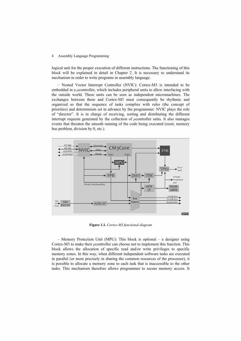
Cortex-M3 targets, in particular, embedded systems requiring significantresources (32-bit), but for these the costs (production, development andconsumption) must be reduced. The first overall illustration (see Figure 1.1) ofCortex-M3, as found in the technical documentation for this product, is a functionaldiagram. Although simple in its representation, every block could perplex a novice.Without knowing all of the details and all of the subtleties, it is useful to have anidea of the main functions performed by different blocks of the architecture.
1.2.1.1. Executive units
These units make up the main part of the processor – the part that is ultimatelynecessary to run applications and to perform them or their software functions:
– CM3CORE: This is the core itself. This unit contains different registers, all ofthe read/write instruction mechanisms and data in the form of the arithmetical and
1 Numbers from the third quarter of 2010.
4 Assembly Language Programming
logical unit for the proper execution of different instructions. The functioning of thisblock will be explained in detail in Chapter 2. It is necessary to understand itsmechanism in order to write programs in assembly language.
– Nested Vector Interrupt Controller (NVIC): Cortex-M3 is intended to beembedded in a μcontroller, which includes peripheral units to allow interfacing withthe outside world. These units can be seen as independent micromachines. Theexchanges between them and Cortex-M3 must consequently be rhythmic andorganized so that the sequence of tasks complies with rules (the concept ofpriorities) and determinism set in advance by the programmer. NVIC plays the roleof “director”. It is in charge of receiving, sorting and distributing the differentinterrupt requests generated by the collection of μcontroller units. It also managesevents that threaten the smooth running of the code being executed (reset, memorybus problem, division by 0, etc.).
Figure 1.1. Cortex-M3 functional diagram
– Memory Protection Unit (MPU): This block is optional – a designer usingCortex-M3 to make their μcontroller can choose not to implement this function. Thisblock allows the allocation of specific read and/or write privileges to specificmemory zones. In this way, when different independent software tasks are executedin parallel (or more precisely in sharing the common resources of the processor), itis possible to allocate a memory zone to each task that is inaccessible to the othertasks. This mechanism therefore allows programmer to secure memory access. It
Overview of Cortex-M3 Architecture 5
usually goes hand-in-hand with the use of an operating system (real-time orotherwise) for the software layer.
– Bus matrix: This unit is a kind of gigantic intelligent multiplex. It allowsconnections to the external buses:
- the ICode bus (32-bit AHB-Lite type2) that carries the memory mappingsallocated to the code and instructions;
- the DCode bus (also 32-bit AHB-Lite type) that is responsible forreading/writing in data memory zones;
- the System bus (again 32-bit AHB-Lite type), which deals with all systemspace access;
- the Private Peripheral Bus (PPB): all peripherals contained in the μcontrollerare added to the Cortex-M3 architecture by the designer. ARM designed a specificbus to allow exchanges with peripherals. This bus contains 32 bits, but in this case itis the Advanced Peripheral Bus (APB) type. This corresponds to another busprotocol (which you may know is less efficient than AHB type, but it is more thansufficient for access to peripheral units). It should be noted that the bus matrix playsan important role in transmitting useful information to development units, which arementioned in the next section.
1.2.1.2. Development units
The development of programs is an important and particularly time-consumingstep in the development cycle of an embedded application. What is more, if theproject has certification imperatives, it is necessary that tools (software and/ormaterial) allowing maximum monitoring of the events occurring in each clock cycleare at its disposition. In Cortex-M3, the different units briefly introduced belowcorrespond to these monitoring functions. They are directly implanted in the siliconof the circuit, which allows them to use these development tools at a material level.An external software layer is necessary, however, to recover and process theinformation issued by these units. The generic idea behind the introduction ofhardware solutions is to offer the programmer the ability to test and improve thereliability of (or certify) his or her code without making any changes. It isconvenient (and usual) to insert some print (“Hello I was here”) into a softwarestructure to check that the execution passes through this structure. This done, a codemodification is introduced, which can modify the global behavior of the program.This is particularly true when time management is critical for the system, which, for
2 Advanced High-performance Bus (AHB) is a microcontroller bus protocol brought in byARM.
6 Assembly Language Programming
embedded systems controlled by a μcontroller, is almost always the case. The unitsrelating to monitoring functions in Cortex-M3 include:
– Flash Patch and Breakpoint (FPB): the FPB is the most basic function for thisprocess. It is linked to the concept of a stopping point (breakpoint), which imposes astop on a line of code (that is to say, an instruction in the case of assembly language)located beforehand. This unit is used to mark instructions so that when they comeinto effect, the processor puts itself into a particular mode of operation: debug mode.Development software (and other pieces of software that use it) can thereforeobserve the state of the processor and directly influence the running of the programin progress.
– Data Watchpoint and Trace (DWT): the concept of a “point of observation” isthe counterpart to the concept of a stopping point for the data. The DWT stops theprogram running when it works on marked data rather than a marked instruction.This action can be in reading, writing, passing on values, etc. The unit can also sendrequests to the ITM and ETM units.
– Embedded Trace Macrocell (ETM): the concept of trace includes the capacityfor the hardware to record a sequence of events during program execution. Therecovery of these recordings allows the programmer to analyze the running of theprogram, whether good or bad. In the case of ETM, only information on instructionsis stored in a first in, first out (FIFO)-type structure. As with the MPU unit, this unitis optional.
– Instrumentation Trace Macrocell (ITM): this unit also allows the collection oftrace information on applications (software, hardware or time). The information ismore limited than with the ETM unit but is nevertheless very useful in isolating avicious bug. This is especially true if the optional ETM is not present.
– Advanced High-performance Bus Access Port (AHB-AP): this is an(Input/Output) port within Cortex-M3 that is designed to debug. It allows access toall records and all addressable memory space. It has priority in the arbitrationpolicies of the bus matrix. This unit is connected upstream by the Serial Wire JTAG(Joint Test Action Group) port (SW/JTAG), which is the interface (with its physicallayers) that connects to the outside world, equipped with its part of the JTAG probe.The JTAG protocol is a standardized protocol used by almost all semiconductormanufacturers.
– Trace Port Interface Unit (TPUI): the TPUI plays the same role in tracefunctions as the SW/JTAG plays in debug functions. Its existence is principallylinked to the fact that it is necessary to sort the external world recordings collectedby the ITM. There is an additional challenge, however, when an ETM unit ispresent, as it must also manage the data stored there. Its secondary role is
Overview of Cortex-M3 Architecture 7
therefore to combine and format this double stream of data before transmitting itto the port. In the outside world, it is necessary to use a Trace Port Analyzer torecover the data.
1.2.2. The Cortex-M3 core in STM32
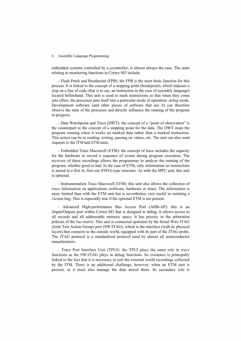
As already stated, ARM does not directly make semiconductors. The μcontrollercore designs are sold under license to designers, who add all of the peripheral unitsthat make up the “interface with the exterior”. For example, the STM32 family ofμcontrollers, made by STMicroelectronics, contains the best selling μcontrollersusing Cortex-M3. Like any good family of μcontrollers, the STM32 family isavailable in many versions. In early 2010, the STMicroelectronics catalog offeredthe products shown in Figure 1.2.
Figure 1.2. STM32 family products
8 Assembly Language Programming
1.2.2.1. Functionality
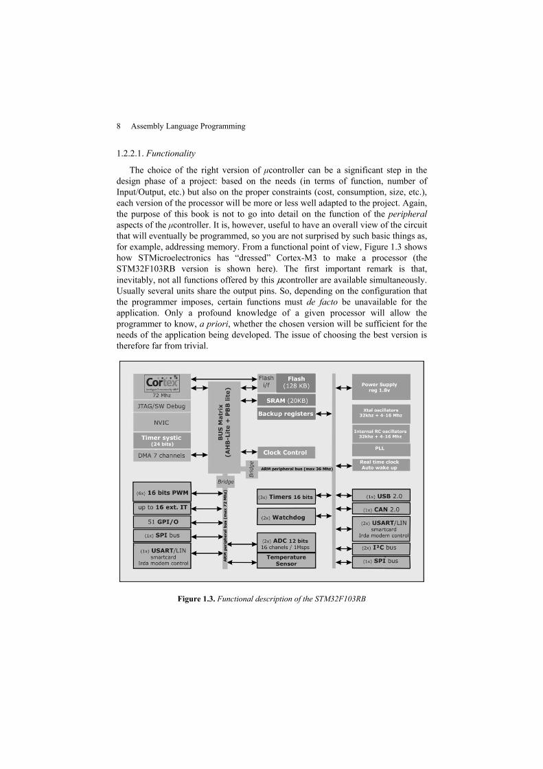
The choice of the right version of μcontroller can be a significant step in thedesign phase of a project: based on the needs (in terms of function, number ofInput/Output, etc.) but also on the proper constraints (cost, consumption, size, etc.),each version of the processor will be more or less well adapted to the project. Again,the purpose of this book is not to go into detail on the function of the peripheralaspects of the μcontroller. It is, however, useful to have an overall view of the circuitthat will eventually be programmed, so you are not surprised by such basic things as,for example, addressing memory. From a functional point of view, Figure 1.3 showshow STMicroelectronics has “dressed” Cortex-M3 to make a processor (theSTM32F103RB version is shown here). The first important remark is that,inevitably, not all functions offered by this μcontroller are available simultaneously.Usually several units share the output pins. So, depending on the configuration thatthe programmer imposes, certain functions must de facto be unavailable for theapplication. Only a profound knowledge of a given processor will allow theprogrammer to know, a priori, whether the chosen version will be sufficient for theneeds of the application being developed. The issue of choosing the best version istherefore far from trivial.
Figure 1.3. Functional description of the STM32F103RB
Overview of Cortex-M3 Architecture 9
In looking at the outline of the STM32F103RB processor, we can see that it hasARM design elements in its processor core, namely:
– a power stage and so clock circuits. This makes it possible to put the processorinto “sleep” mode and allow access to different frequencies (which is interesting fortimer management in particular);
– the addition of Flash and RAM. The amount of memory present in the case isone of the variables that fluctuates the most, depending on which μcontroller ischosen. The STM32F103RB version has 128 KB of Flash memory which, to put itin perspective, can represent up to 65,000 lines of code written in assembly language(assuming that an instruction is coded on 16 bits);
– managers developed in system time, including the Systick 24-bit timer and anautomatic wake-up system when the processor has gone into “sleep” mode. Theseunits have an undeniable usefulness during the use of the real-time kernel.
STMicroelectronics then added the following functions:
– time and/or counting management peripherals;
– analog signal management peripherals. These are analogical/numericalconverters for acquiring analog quantities, and represent the PWM (Pulse WidthModulation) managers for sending assimilable signals to the analog quantities;
– digital input/output peripherals. These 51 General Purpose Input Output(GPIO) peripherals are the TTL (Transistor-Transistor Logic) input/output ports andthe other 16 signals involving digital input that can transmit an interrupt request;
– communication peripherals. Different current protocols are present in this chipfor communications via a serial link (Universal Synchronous AsynchronousReceiver Transmitter (USART)), Universal Serial Bus (USB) or an industrial bus(I2C, Controller–area network (CAN), Serial Peripheral Interface (SPI)).
1.2.2.2.Memory space
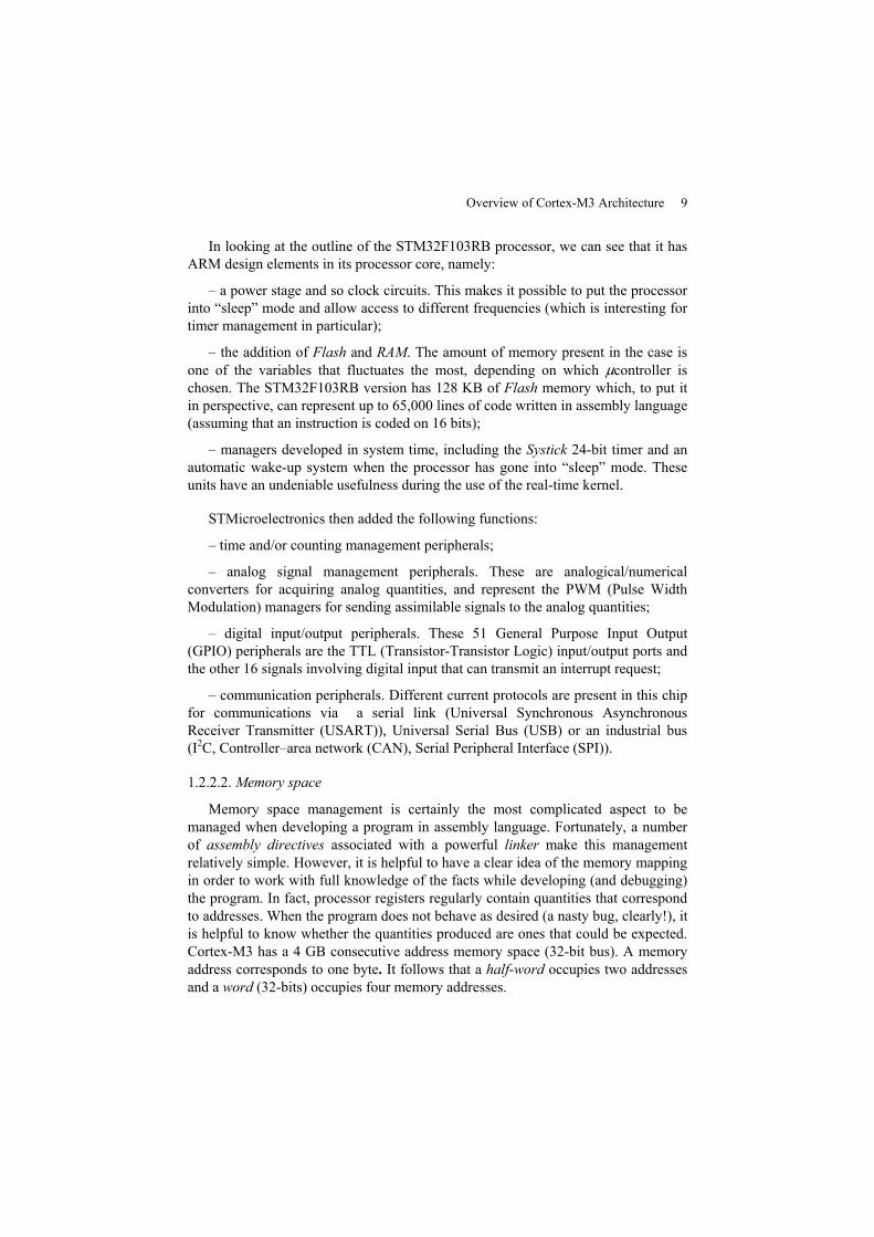
Memory space management is certainly the most complicated aspect to bemanaged when developing a program in assembly language. Fortunately, a numberof assembly directives associated with a powerful linker make this managementrelatively simple. However, it is helpful to have a clear idea of the memory mappingin order to work with full knowledge of the facts while developing (and debugging)the program. In fact, processor registers regularly contain quantities that correspondto addresses. When the program does not behave as desired (a nasty bug, clearly!), itis helpful to know whether the quantities produced are ones that could be expected.Cortex-M3 has a 4 GB consecutive address memory space (32-bit bus). A memoryaddress corresponds to one byte. It follows that a half-word occupies two addressesand a word (32-bits) occupies four memory addresses.
10 Assembly Language Programming
By convention, data storage is arranged according to the little endian standard,where the least significant byte of a word or half-word is stored at the lowestaddress, and we return to the higher addresses by taking the series of componentbytes making up the numbers stored in memory. Figure 1.4 shows how, in the littleendian standard, memory placement of words and half-words is managed.
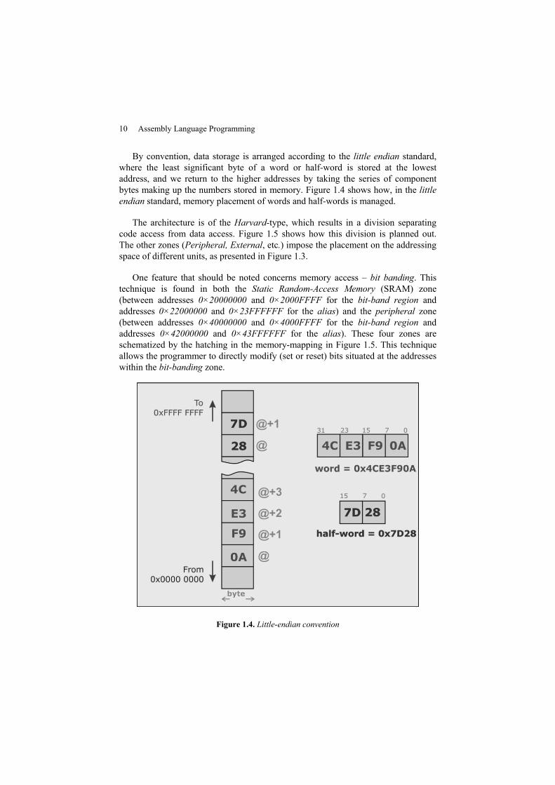
The architecture is of the Harvard-type, which results in a division separatingcode access from data access. Figure 1.5 shows how this division is planned out.The other zones (Peripheral, External, etc.) impose the placement on the addressingspace of different units, as presented in Figure 1.3.
One feature that should be noted concerns memory access – bit banding. Thistechnique is found in both the Static Random-Access Memory (SRAM) zone(between addresses 0×20000000 and 0×2000FFFF for the bit-band region andaddresses 0×22000000 and 0×23FFFFFF for the alias) and the peripheral zone(between addresses 0×40000000 and 0×4000FFFF for the bit-band region andaddresses 0×42000000 and 0×43FFFFFF for the alias). These four zones areschematized by the hatching in the memory-mapping in Figure 1.5. This techniqueallows the programmer to directly modify (set or reset) bits situated at the addresseswithin the bit-banding zone.
Figure 1.4. Little-endian convention
Overview of Cortex-M3 Architecture 11
Figure 1.5. Cortex-M3 memory mapping
12 Assembly Language Programming
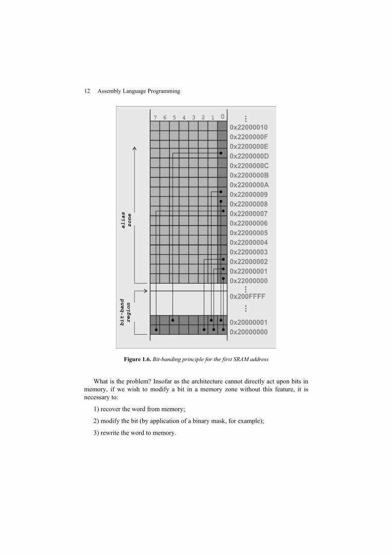
Figure 1.6. Bit-banding principle for the first SRAM address
What is the problem? Insofar as the architecture cannot directly act upon bits inmemory, if we wish to modify a bit in a memory zone without this feature, it isnecessary to:
1) recover the word from memory;
2) modify the bit (by application of a binary mask, for example);
3) rewrite the word to memory.
Overview of Cortex-M3 Architecture 13
ARM is designed to match the address of a word (in the alias zone) with a bit (inthe bit-banding zone). So when the programmer writes a value in the alias zone, itamounts to modifying the bit-banding bit corresponding to the zero-weight bit thatthey just wrote. Conversely, reading the least significant bit of a word in the aliaszone lets the programmer know the logic state of the corresponding bit in thebit-banding zone (see Figure 1.6). It should be noted that this technique does not useRAM memory insofar as alias zones are imaginary: they do not physicallycorrespond to memory locations – they only use memory addresses, but with 4 GBof possible addresses this loss is of little consequence.

Chapter 2
The Core of Cortex-M3
The previous chapter showed how the programmer could break down thedifferent units present in a μcontroller like STM32 from a functional point of view.It is now time to delve a little deeper into the Cortex-M3 core, and to explain indetail the contents of the CM3CORE box, as shown in Figure 2.1.
It would be pointless to create a replica (which would be incomplete due to thesimplification necessary) of the contents of the various reference manuals[ARM 06a, ARM 06b, ARM 06c] that give detailed explanations of Cortexfunctions. It would also be pointless, however, to claim to program in assemblylanguage without having a reasonably precise idea of its structure. This chaptertherefore attempts to present the aspects of the architecture necessary for reasonedprogramming of a μcontroller.
2.1. Modes, privileges and states
Cortex-M3 can be put into two different operating modes: thread mode andHandler mode. These modes combine with the privilege levels that can be granted tothe execution of a program regarding access to certain registers:
– At the unprivileged access level, the executed code cannot access allinstructions (those instructions specific to the access of special registers areexcluded). It does not generally have access to all functions within the system(Nested Vector Interrupt Controller [NVIC], timer system, etc.). The concern issimply to avoid having code that, by bad management of a pointer for example,would be detrimental to the global behavior of the processor and severely disturb therunning of the application.
16 Assembly Language Programming
– At the other end of the spectrum, at the privileged level, all of these limitationsare lifted.
– Thread mode corresponds to the default mode in the sense that it is the modethat the processor takes after being reset. It is the normal mode for the execution ofapplications. In this mode, both privilege levels are possible.
– The processor goes into Handler mode following an exception. When it hasfinished processing the instructions for this exception, the last instruction allows areturn to normal execution and causes the return to thread mode. In this mode, thecode always has privileged level access.
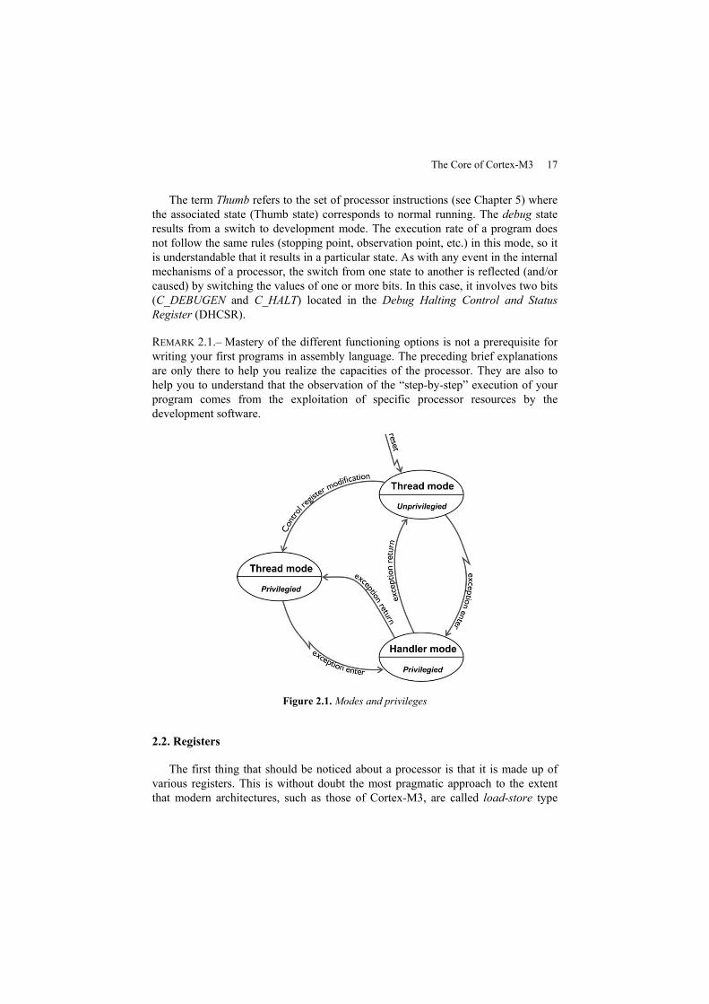
Passage between these three types of functioning can be described by a statemachine, see Figure 2.1 [YIU 07]. After being reset, the processor is in thread modewith privilege. By setting the least significant bit (LSB) of the CONTROL register, itis possible to switch into unprivileged mode (also called user mode in the ARMdocumentation) using software. In unprivileged mode, the user cannot access theCONTROL register, and so it is impossible to return to the privileged mode. Justafter the launch of an exception (see Chapter 8) the processor switches to Handlermode, which necessarily has privilege. Once the exception has been processed, theprocessor returns to its previous mode. If, during processing of the exception, theLSB of the CONTROL register is modified, then the processor can return to theopposite mode to that which was in effect before the launch. The only way to switchto unprivileged thread mode, as opposed to privileged thread mode, is by goingthrough an exception that expresses itself by passing into Handler mode.
This level of protection can appear somewhat minimalist. It is a little like thelocking/unlocking of your mobile phone: it takes a combination of keys (known toall) to achieve. It is obviously no use in preventing theft, but it is still useful whenthe phone is in the bottom of a pocket.
This type of security can only be developed within a global software architectureincluding an operating system. In a rather simplistic but ultimately quite realisticmanner, it is possible to imagine that the operating system (OS) has full accessprivileges. It can therefore launch tasks in unprivileged thread mode, which couldguarantee an initial level of security. A second privilege level concerns the functionsof the memory protection unit block mentioned previously. Each task can onlyaccess the memory regions assigned to it by the OS.
A supplementary element should be taken into account in order to understand thefunctioning of Cortex-M3. It concerns the internal state of the processor, which canbe in either Thumb or debug state.
The Core of Cortex-M3 17
The term Thumb refers to the set of processor instructions (see Chapter 5) wherethe associated state (Thumb state) corresponds to normal running. The debug stateresults from a switch to development mode. The execution rate of a program doesnot follow the same rules (stopping point, observation point, etc.) in this mode, so itis understandable that it results in a particular state. As with any event in the internalmechanisms of a processor, the switch from one state to another is reflected (and/orcaused) by switching the values of one or more bits. In this case, it involves two bits(C_DEBUGEN and C_HALT) located in the Debug Halting Control and StatusRegister (DHCSR).
REMARK 2.1.– Mastery of the different functioning options is not a prerequisite forwriting your first programs in assembly language. The preceding brief explanationsare only there to help you realize the capacities of the processor. They are also tohelp you to understand that the observation of the “step-by-step” execution of yourprogram comes from the exploitation of specific processor resources by thedevelopment software.
Figure 2.1. Modes and privileges
2.2. Registers
The first thing that should be noticed about a processor is that it is made up ofvarious registers. This is without doubt the most pragmatic approach to the extentthat modern architectures, such as those of Cortex-M3, are called load-store type
18 Assembly Language Programming
architectures. This means that the programs initially transfer data from memory tothe registers and performs operations on these registers in a second step. Finally, andwhen necessary, there is the transfer of the result to memory.
First we must define what a register is. A register, in the primary sense,corresponds to the location in internal memory (in the sense of a series of accessiblebits in parallel) of a processor. We should, however, adjust this definition for thesimple reason that, in the case of a μcontroller, although there is internal memory(20 KB of static RAM in the case of a standard STM32, and that is without takinginto account Flash memory), this internal memory does not make up a set ofregisters. An equally inexact definition would be to think of a register as a memorylocation that does not take part in memory mapping. In effect, all peripherals of acontroller can be programmed by means of the values that they are given by theregisters; they have no fewer physical addresses that the processor can access thanany other memory space. The extensive use of the term “register” in computerarchitecture means that this term often encompasses, in a rather vague manner, allmemory spaces whose content directly affects the functioning of the processor. Inthis section, we will only consider the registers of the Cortex-M3 core. Their mainfeature is that they are accessible by the instruction set without submitting a requestto the data bus. The opcode (which is linked to the coding of the instruction to beexecuted) of an instruction manipulating the contents of a register must thereforecontain the information of the register to be contacted. The execution of aninstruction can cause the modification of one or more of these registers without theneed to activate the data bus.
Conrtex-M3 has 17 initial registers, all obviously 32-bit:
– R0 to R12: 13 general usage registers;
– R13: a stack pointer register, also called SP, PSP (SP_process) or MSP(SP_main);
– R14: link register (LR);
– R15: ordinal counter or PC (program pointer);
– xPSR: a state register (Program Status Register, the x can be A forApplication, I for Interrupt or E for Execution) that is strangely never called R16.
To these 17 registers we must add three special registers (PRIMASK,FAULTMASK and BASEPRI), which are used for exception handling (seeChapter 8). The 21st that we can add to this list is the CONTROL register, which hasalready been mentioned for its role in privilege levels but which is also a level of theR13 stack pointer.
The Core of Cortex-M3 19
2.2.1. Registers R0 to R12
These 13 registers are used, as we shall see in the passage reviewing theinstruction set, as a container for storing the operands of an instruction and toreceive the results of these operations. ARM distinguishes between the first eightregisters R0 to R7 (low registers) and the following four (R8 to R12, the highregisters). The high registers have employment restrictions with respect to certaininstructions. The prudent programmer will primarily use the first eight registers sothat they do not have to manage these restrictions.
REMARK 2.2.– These general registers, contrary to other architectures, are onlyaccessible in 32-bit packets. The registers can therefore not be split into two half-words or four bytes. If your application deals with bytes (chains of characters to bemore precise), for example, the 24 highest weighted bits would be positioned at 0 inorder for their operation to be sensible.
2.2.2. The R13 register, also known as SP
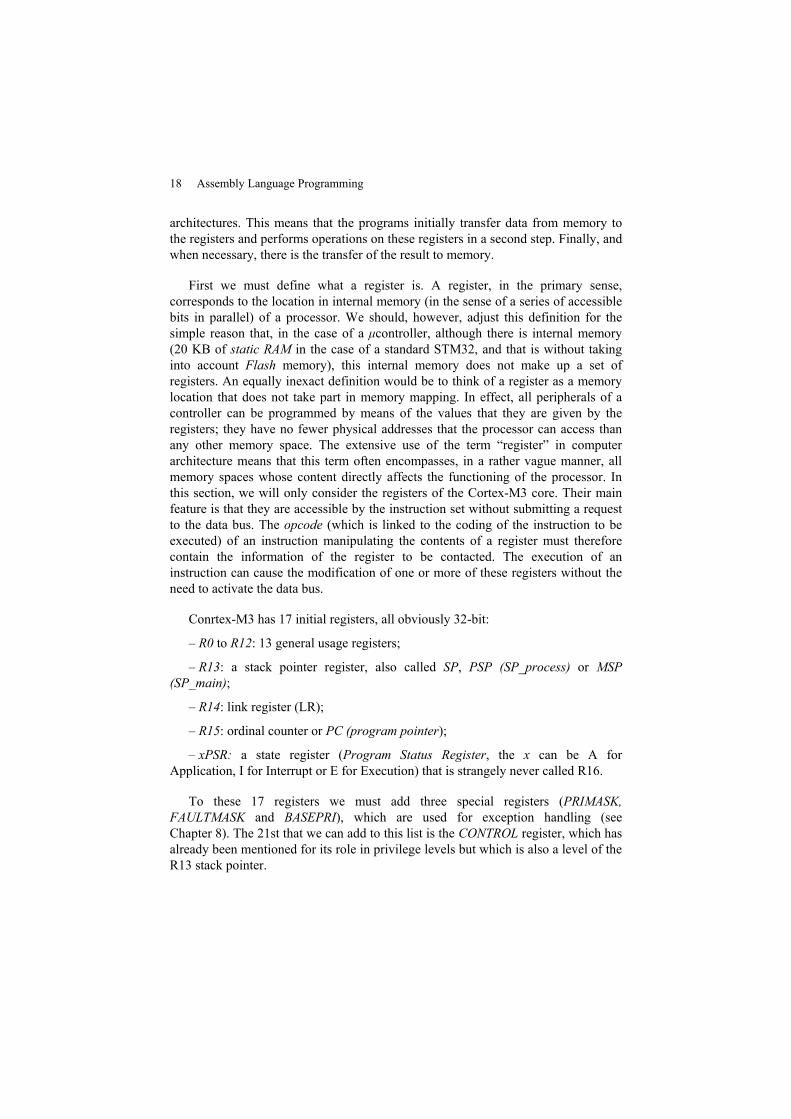
R13 is the SP register. As its name suggests, it points (i.e. it contains the addressof a memory location) to a place that corresponds to the current location of thesystem stack. This idea of a stack will be explained in more detail later (see section6.5.6), but for now we will just consider it as a buffer zone where the runningprogram can temporarily store data. In the case of Cortex-M3, this storage zone isdoubled, and so the SP register comes in two versions: PSP (SP_Process) or MSP(SP_Main). It is important to note that, at any given moment, only one of the twostacks is visible to the processor. So when writing to the stack as in the followingexample:
EXAMPLE 2.1.– Saving a register
PUSH R14 ; PC save
; MSP or PSP???
The writing is done to the visible zone. In terms of this visibility, we can acceptthat, in Handler mode, the current pointer is always MSP. In thread mode, even if itcan be modified with software, the current pointer is PSP. Thus, without particularmanipulation, access to the system stack will be via PSP during the normal course ofthe program, but when there is an exception the management of the stack is subjectto MSP. This division induces a much greater reliability in the functioning of theμcontroller and greater speed during context changes (not forgetting that the
20 Assembly Language Programming
peripherals communicate with Cortex-M3 through interruptions and so an exceptionis not exceptional, etc.).
Figure 2.2. Double stack system
2.2.3. The R14 register, also known as LR
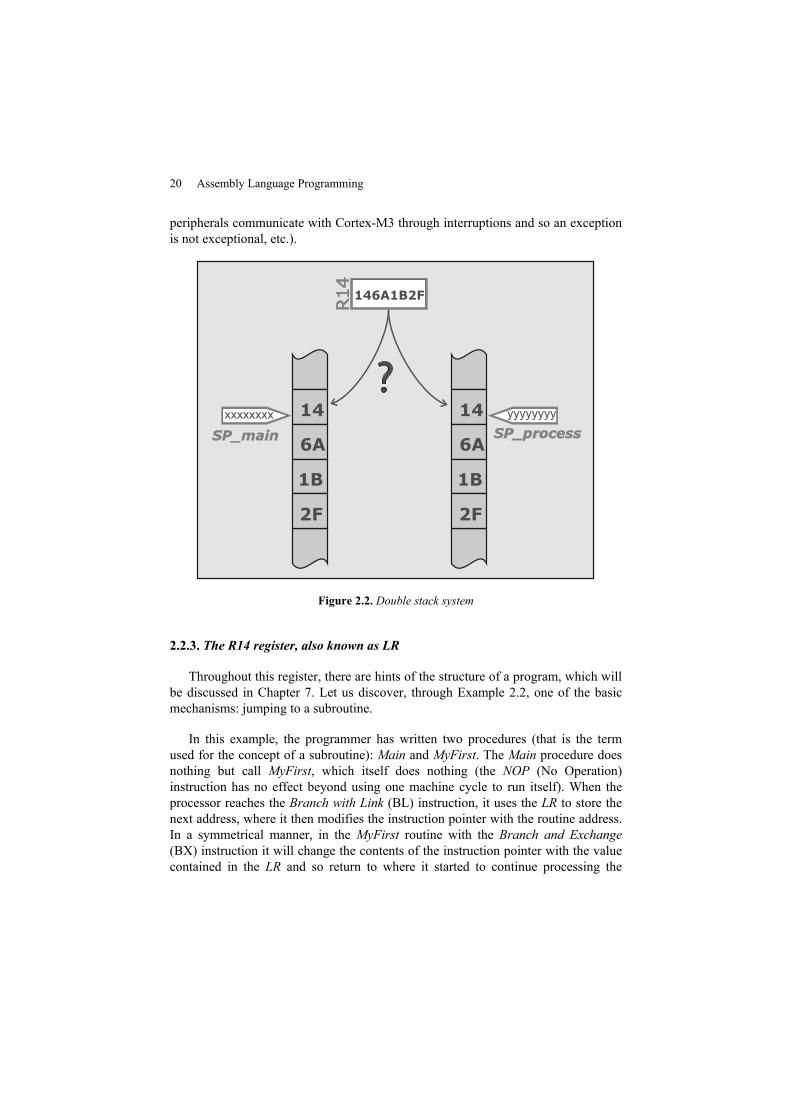
Throughout this register, there are hints of the structure of a program, which willbe discussed in Chapter 7. Let us discover, through Example 2.2, one of the basicmechanisms: jumping to a subroutine.
In this example, the programmer has written two procedures (that is the termused for the concept of a subroutine): Main and MyFirst. The Main procedure doesnothing but call MyFirst, which itself does nothing (the NOP (No Operation)instruction has no effect beyond using one machine cycle to run itself). When theprocessor reaches the Branch with Link (BL) instruction, it uses the LR to store thenext address, where it then modifies the instruction pointer with the routine address.In a symmetrical manner, in the MyFirst routine with the Branch and Exchange(BX) instruction it will change the contents of the instruction pointer with the valuecontained in the LR and so return to where it started to continue processing the
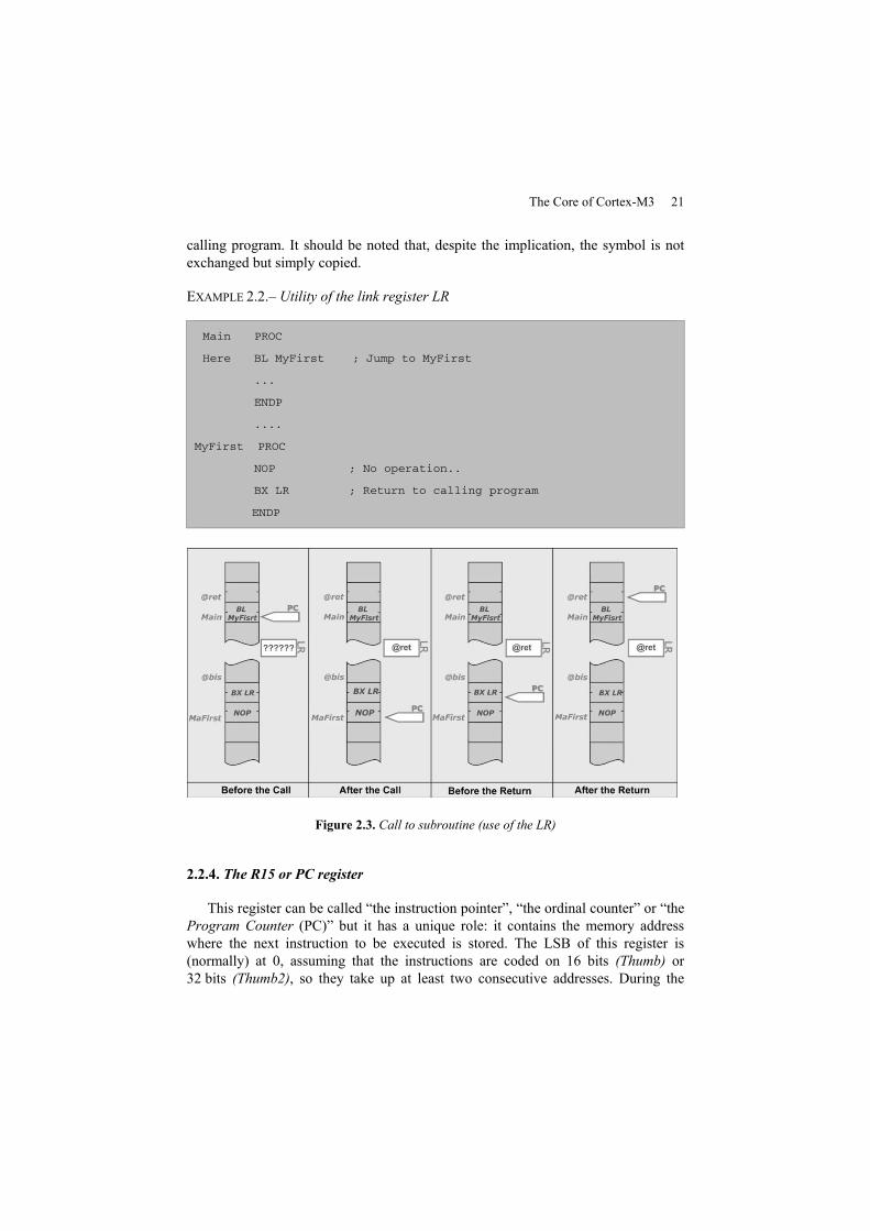
The Core of Cortex-M3 21
calling program. It should be noted that, despite the implication, the symbol is notexchanged but simply copied.
EXAMPLE 2.2.– Utility of the link register LR
Main PROC
Here BL MyFirst ; Jump to MyFirst
...
ENDP
....
MyFirst PROC
NOP ; No operation..
BX LR ; Return to calling program
ENDP
Figure 2.3. Call to subroutine (use of the LR)
2.2.4. The R15 or PC register
This register can be called “the instruction pointer”, “the ordinal counter” or “theProgram Counter (PC)” but it has a unique role: it contains the memory addresswhere the next instruction to be executed is stored. The LSB of this register is(normally) at 0, assuming that the instructions are coded on 16 bits (Thumb) or32 bits (Thumb2), so they take up at least two consecutive addresses. During the
22 Assembly Language Programming
running of a code sequence, the PC pointer will automatically increment itself(usually two-by-two) in order to then point and recover the rest of the code. Theterm ordinal counter could imply that its functioning is limited to this simpleincrementation. This is not so, and things quickly become complicated, particularlywhen there is a break in the sequence (in the instance of Example 2.2, where the callto a subroutine caused a discontinuity in the rest of the stored code addresses). Inthis case, PC would take a value that was not a simple incrementation of its initialvalue.
The management of this pointer is intrinsically linked to the pipeline structure ofthis Reduced Instruction Set Computer (RISC) architecture. This technique allowsthe introduction of a form of parallelism in the work of the processor. At eachmoment, several instructions are processed simultaneously, each at a different level.Three successive steps are necessary for an instruction to be completely carried out:
– The Fetch phase: recovery of the instruction from memory. This is the stepwhere PC plays its part.
– The Decode phase: the instruction is a value encoded in memory (its opcode),which requires decoding to prepare it for execution (data recovery, for example).
– The Execute phase: execution of the decoded instruction and writing back ofthe results if necessary.
In these three stages (which are classic in a pipeline structure) a first upstreamunit must be added: the PreFetch unit. This unit (which is part of ARM’s expertise)essentially exists to predict what will happen during sequence breaks and to prepareto recover the next instruction by “buffering” about six instructions in advance. Thispractice optimizes processor speed.
This simplified view of pipeline stages deliberately masks its complexity. Again,in line with the objectives of this book, this level of understanding is sufficient towrite programs in assembly language. Interested readers can search the ARMdocumentation to find all of the explanations necessary to go further.
2.2.5. The xPSR register
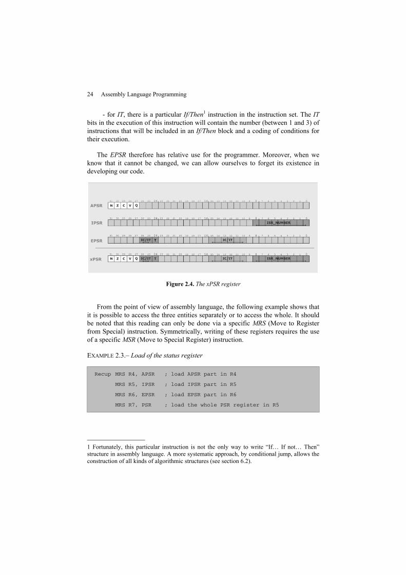
This register contains information regarding the “status” or “state” of theprocessor. It contains important information – a kind of short report – about whathas happened in the processor. It is available in three versions, although it is onlyone register. The distribution of significant bits, as shown in Figure 2.4, is such thatthere is no intersection, so it is possible to separate it into three independent subsets:
The Core of Cortex-M3 23
– APSR, with the A meaning Application: this register contains the flags of theprocessor. These five bits are essential for the use of conditional operations, sincethe conditions exclusively express themselves as a logical combination of theseflags. Updating of these is carried out by most of the instructions, provided that thesuffix S is specified in the symbolic name of the instruction. These flags are:
- indicator C (Carry): represents the “carry” during the calculation of thenatural (unsigned) quantities. If C=1, then there was an overflow in the unsignedrepresentation during the previous instruction, which shows that the unsigned resultis partially false. Knowledge of this bit allows for much more precise work;
- indicator Z (Zero): has a value of 1 if the result is zero;
- indicator N (Negative): copies the most significant bit of the result. If thevalue is signed, N being 1 therefore indicates a negative result;
- indicator V (oVerflow): if this has a value of 1, there has been an overflow (orunderflow) of signed representation. The signed result is false;
- indicator Q (Sticky Saturation Flag): only makes sense for the two specificsaturation instructions USAT and SSAT: the bit is set at 1 if these instructions havesaturated the register used.
– IPSR, with the I meaning Interrupt: in this configuration, this refers to the nineLSBs containing information. These nine bits make up the exception number(Interrupt Service Routine or ISR) that will be launched. For example, when the ISRhas a value of 2, it corresponds to the launch of a Non Maskable Interrupt (NMI)interruption; if it has a value of 5 then there has been a problem with memoryaccess.
– EPSR, with the E meaning Execution: this register stores three distinct piecesof information:
- the 24-bit (T) to indicate whether it is in Thumb state – that is, if it is usingthe Thumb instruction set. As this is always the case, this bit is always at 1. Wecould question the usefulness of this information. As a matter of fact, it is useless inthe case of Cortex-M3, but in other architectures this bit can be at 0 to show that theprocessor is using the ARM set and not Thumb;
- it uses bit fields [10–15] and [25–26] to store two pieces of overlappinginformation (the two uses are mutually exclusive): ICI or IT;
- for ICI, this is information that is stored when a read/write multiple (theprocessor reads/writes several general registers successively, but uses only oneinstruction) is interrupted. Upon returning from the interruption, the processor canresume its multiple accesses from where it was before;
24 Assembly Language Programming
- for IT, there is a particular If/Then1 instruction in the instruction set. The ITbits in the execution of this instruction will contain the number (between 1 and 3) ofinstructions that will be included in an If/Then block and a coding of conditions fortheir execution.
The EPSR therefore has relative use for the programmer. Moreover, when weknow that it cannot be changed, we can allow ourselves to forget its existence indeveloping our code.
Figure 2.4. The xPSR register
From the point of view of assembly language, the following example shows thatit is possible to access the three entities separately or to access the whole. It shouldbe noted that this reading can only be done via a specific MRS (Move to Registerfrom Special) instruction. Symmetrically, writing of these registers requires the useof a specificMSR (Move to Special Register) instruction.
EXAMPLE 2.3.– Load of the status register
Recup MRS R4, APSR ; load APSR part in R4
MRS R5, IPSR ; load IPSR part in R5
MRS R6, EPSR ; load EPSR part in R6
MRS R7, PSR ; load the whole PSR register in R5
1 Fortunately, this particular instruction is not the only way to write “If… If not… Then”structure in assembly language. A more systematic approach, by conditional jump, allows theconstruction of all kinds of algorithmic structures (see section 6.2).
Chapter 3
The Proper Use of Assembly Directives
As for any language, the syntactic aspect of a listing is of crucial importance sothat the compiler (in the case of higher level language structures) or the assembler(for listings written in assembly language) understands the rest of the characters thatit will read and that make up the program. If we consider the previous examples, anassembler would have trouble generating the corresponding executable code: it lacksa lot of information. Only a few instructions, without any context, were transcribedin the examples that have previously been presented. Where is the code entry point,where does the program end, where is the code located in memory, what are theconstants or variables?
This chapter aims to define this context through the description of assemblydirectives.
3.1. The concept of the directive
An assembly directive is a piece of information that appears word-for-word inthe listing and which is supplied by the assembler to give the construction rules ofthe executable. These lines in the source file, though an integral part of the listingand necessary for its coherence, do not correspond directly to any line of code.These pieces of information will therefore not appear during the disassembly of thecode and will be also be missing if a hacker tries to reverse engineer it. Disassemblyis a process that consists of converting the code (that is, the collection of words readin memory) into the corresponding symbols and, if necessary, the operands (numericor register). The coding of an instruction being biunivocal, there is no particularproblem in re-transcribing a code extracted from memory into primitive assembly
26 Assembly Language Programming
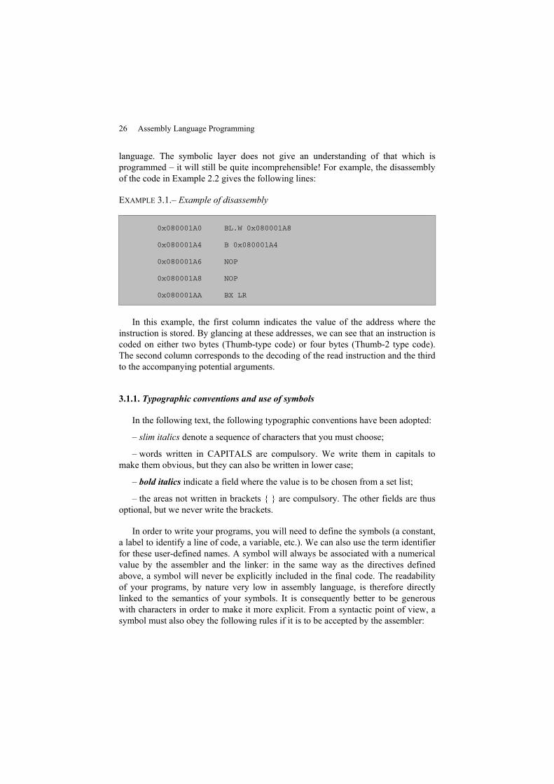
language. The symbolic layer does not give an understanding of that which isprogrammed – it will still be quite incomprehensible! For example, the disassemblyof the code in Example 2.2 gives the following lines:
EXAMPLE 3.1.– Example of disassembly
0x080001A0 BL.W 0x080001A8
0x080001A4 B 0x080001A4
0x080001A6 NOP
0x080001A8 NOP
0x080001AA BX LR
In this example, the first column indicates the value of the address where theinstruction is stored. By glancing at these addresses, we can see that an instruction iscoded on either two bytes (Thumb-type code) or four bytes (Thumb-2 type code).The second column corresponds to the decoding of the read instruction and the thirdto the accompanying potential arguments.
3.1.1. Typographic conventions and use of symbols
In the following text, the following typographic conventions have been adopted:
– slim italics denote a sequence of characters that you must choose;
– words written in CAPITALS are compulsory. We write them in capitals tomake them obvious, but they can also be written in lower case;
– bold italics indicate a field where the value is to be chosen from a set list;
– the areas not written in brackets { } are compulsory. The other fields are thusoptional, but we never write the brackets.
In order to write your programs, you will need to define the symbols (a constant,a label to identify a line of code, a variable, etc.). We can also use the term identifierfor these user-defined names. A symbol will always be associated with a numericalvalue by the assembler and the linker: in the same way as the directives definedabove, a symbol will never be explicitly included in the final code. The readabilityof your programs, by nature very low in assembly language, is therefore directlylinked to the semantics of your symbols. It is consequently better to be generouswith characters in order to make it more explicit. From a syntactic point of view, asymbol must also obey the following rules if it is to be accepted by the assembler:
The Proper use of Assembly Directives 27
– the name of a symbol must be unique within a given module;
– the characters may be upper or lower case letters, numbers or “underscores”.The assembler is case-sensitive;
– a priori, there is no maximum length;
– the first character cannot be a number;
– the key words (mnemonics, directives, etc.) of the language are reserved;
– if it proves necessary to use a palette of more important characters (in order tomix your code with a compiler, for example), it is possible to do this by surroundingthe symbol with | (these do not become part of the symbol). For example |.text| is avalid symbol and the assembler will memorize it (in its symbol table) as .text.
3.2. Structure of a program
Writing a program in assembly language, in its simplest form, implies that theuser can, in a source file (which is just a text file and so a simple series of ASCIIcharacters):
– define the sequence of code instructions, so that the assembler will be able totranslate them into machine language. This sequence, once assembled and givenCortex-M3 Harvard structure, will be stored in CODE memory;
– declare the data it will use, by giving it an initial or constant value, ifnecessary. This allows the assembler to give orders to reserve the necessary memoryspace, by initializing everything that is predestined to fill the DATA memory, whenappropriate.
REMARK 3.1.– A third entity is required for the correct running of a program: thesystem stack. This is not fixed in size or memory location. This implies thatsomewhere in the listing there is a reservation for this specific area and at least oneinstruction for the initialization of the stack pointer (SP) responsible for itsmanagement. In using existing development tools, this phase is often included in afile (written in assembly language) that contains a number of initializations. Indeed,the μcontroller hosting Cortex-M3 must also undergo a number of configurationoperations just after a reset; the initialization of the stack in this file is consequentlynot aberrant. The advanced programmer will, however, have to verify that thepredefined size of the system stack is not under- or over-sized relative to itsapplication.
28 Assembly Language Programming
3.2.1. The AREA sections
A program in assembly language must have at least two parts, which we willrefer to as sections, that must be defined in the listing by the AREA directive:
– one section of code containing the list of instructions;
– one section of data where we find the description of the data (name, size, initialvalue).
REMARK 3.2.– Unlike in higher level languages where the declaration of variablescan be more or less mixed with instructions, assembly language requires a clearseparation.
From the point of view of the assembler, a section is a contiguous zone ofmemory in which all of the elements are of the same logical nature (instructions,data, and system stack).
The programmer uses the AREA directive to communicate with the assembler inorder to show the beginning of a section. The section naturally terminates at thebeginning of another section, so there is no specific marker for the end of a section.
The body of a section is made up of instructions for the CODE part or of variousplace reservations (whether initialized of not) for the DATA section.
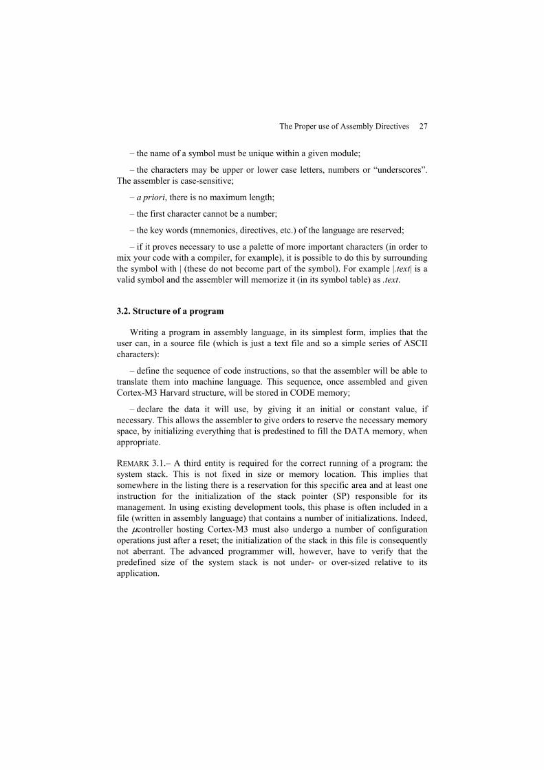
The general definition syntax of a section, as it must be constructed in a sourcefile, is:
AREA Section_Name { ,type } { ,attr } …
… Body of the section:
… definitions of data
… or instructions, according to the case
So let us explain the four fields:
– AREA: the directive itself;
– Section_Name: the name that you have given to the section in keeping with therules set out earlier;
– type: code or data: indicates the type of section being opened;
– a suite of non-compulsory options. The principal options are:
The Proper use of Assembly Directives 29
- readonly or readwrite: indicates whether the section is accessible to readonly (the default for CODE sections) or to read and write (the default for DATAsections),
- noinit: indicates, for a DATA section, that it is not initialized or initialized at0. This type of section can only contain rough memory reservations or reservationsfor data initialized at 0, and
- align = n with a value between 0 and 31. This option indicates how thesection should be placed in memory. The section will be aligned with a 2n moduloaddress, or in other terms it signifies that the least significant n bits of the firstaddress of the section would be at 0.
There are other options which, if they need to be put in place, show that youhave reached a level of expertise beyond the scope of this book.
In a program, a given section can be opened and closed several times. It is alsopossible that we might like to open different sections of code or data that are distinctfrom each other. Finally, all of these various parts combine automatically. That isthe role of the linker, which should therefore take into account the variousconstraints so that it can assign memory addresses for each constituent section of theproject.
3.3. A section of code
A section of code contains instructions in symbolic form. One instruction iswritten on one line, according to the following syntax:
{ label } SYMBOL { expr }{ ,expr }{ ,expr} { ; comment}
The syntax of all assembly language is rigorous. At most, we can place oneinstruction on one line. It is also permitted to have lines without an instructioncontaining a label, a comment or even nothing at all (to space out the listing in orderto make it more readable). Finally, please note that a label must always be placed inthe first column of the line.
3.3.1. Labels
A label is a symbol of your choice that is always constructed according to thesame rules. The label serves as a marker, or an identifier, for the instruction (or thedata). It allows us to go to that instruction during execution by way of a jump (orbranch).
30 Assembly Language Programming
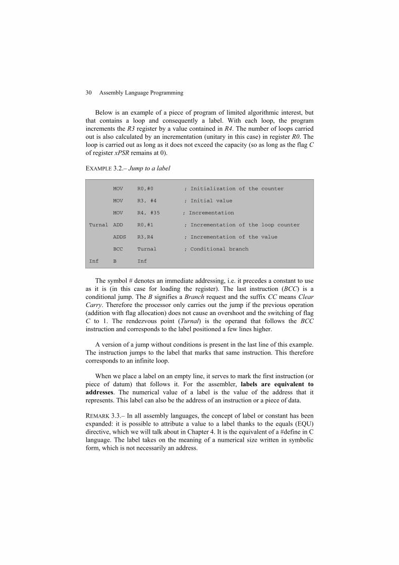
Below is an example of a piece of program of limited algorithmic interest, butthat contains a loop and consequently a label. With each loop, the programincrements the R3 register by a value contained in R4. The number of loops carriedout is also calculated by an incrementation (unitary in this case) in register R0. Theloop is carried out as long as it does not exceed the capacity (so as long as the flag Cof register xPSR remains at 0).
EXAMPLE 3.2.– Jump to a label
MOV R0,#0 ; Initialization of the counter
MOV R3, #4 ; Initial value
MOV R4, #35 ; Incrementation
Turnal ADD R0,#1 ; Incrementation of the loop counter
ADDS R3,R4 ; Incrementation of the value
BCC Turnal ; Conditional branch
Inf B Inf
The symbol # denotes an immediate addressing, i.e. it precedes a constant to useas it is (in this case for loading the register). The last instruction (BCC) is aconditional jump. The B signifies a Branch request and the suffix CC means ClearCarry. Therefore the processor only carries out the jump if the previous operation(addition with flag allocation) does not cause an overshoot and the switching of flagC to 1. The rendezvous point (Turnal) is the operand that follows the BCCinstruction and corresponds to the label positioned a few lines higher.
A version of a jump without conditions is present in the last line of this example.The instruction jumps to the label that marks that same instruction. This thereforecorresponds to an infinite loop.
When we place a label on an empty line, it serves to mark the first instruction (orpiece of datum) that follows it. For the assembler, labels are equivalent toaddresses. The numerical value of a label is the value of the address that itrepresents. This label can also be the address of an instruction or a piece of data.
REMARK 3.3.– In all assembly languages, the concept of label or constant has beenexpanded: it is possible to attribute a value to a label thanks to the equals (EQU)directive, which we will talk about in Chapter 4. It is the equivalent of a #define in Clanguage. The label takes on the meaning of a numerical size written in symbolicform, which is not necessarily an address.
The Proper use of Assembly Directives 31
3.3.2.Mnemonic
We use mnemonic to mean the symbolic name of an instruction. This name is setand the series of mnemonics makes up the instruction set.
In the ARM world, since the ARMV4 version of the architecture, there havebeen two distinct instruction sets: the ARM set (coded in 32 bits) and the Thumb set(coded in 16 bits). The size for coding with the Thumb set being smaller, this setoffers fewer possibilities than the full ARM set. The advantage that can be drawnfrom this compression is a more compact code. For many ARM processors, there isthe option to make them work in Thumb or ARM mode, according to the needs andappropriate constraints of the project.
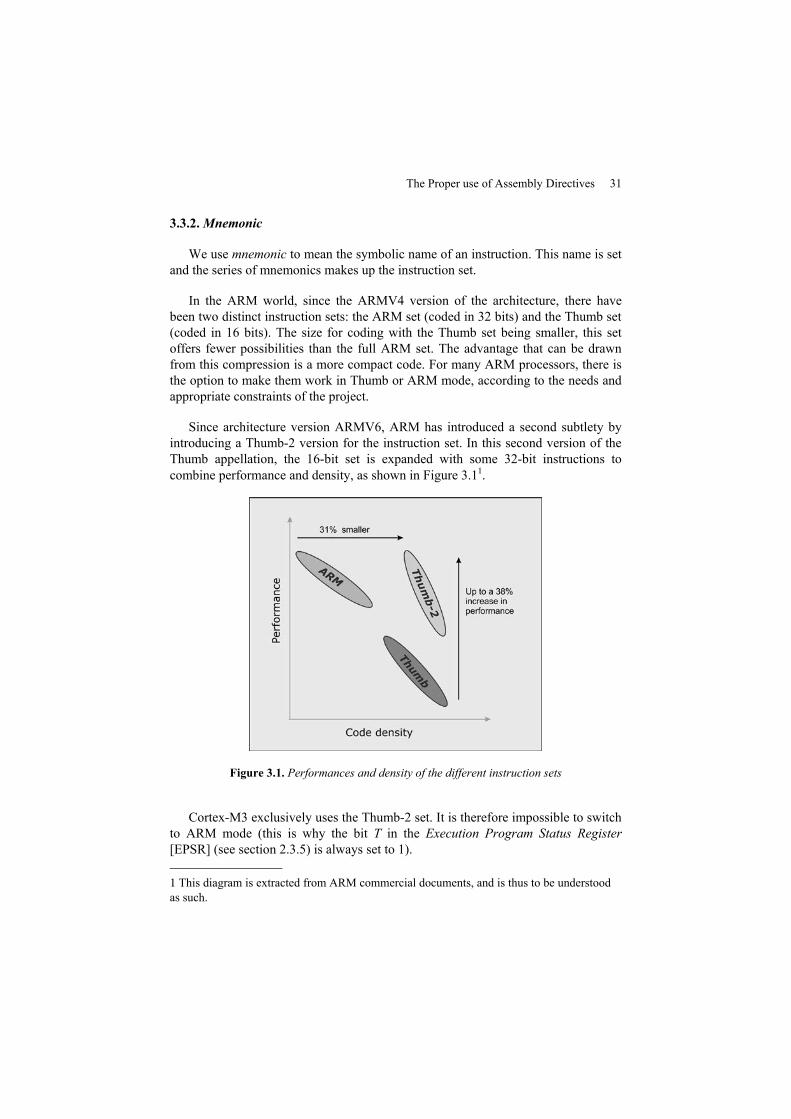
Since architecture version ARMV6, ARM has introduced a second subtlety byintroducing a Thumb-2 version for the instruction set. In this second version of theThumb appellation, the 16-bit set is expanded with some 32-bit instructions tocombine performance and density, as shown in Figure 3.11.
Figure 3.1. Performances and density of the different instruction sets
Cortex-M3 exclusively uses the Thumb-2 set. It is therefore impossible to switchto ARM mode (this is why the bit T in the Execution Program Status Register[EPSR] (see section 2.3.5) is always set to 1).
1 This diagram is extracted from ARM commercial documents, and is thus to be understoodas such.
32 Assembly Language Programming
The Thumb-2 set understands 114 different mnemonics (excludingcommunication instructions with a potential coprocessor). A quick classificationallows us to pick out:
– 8 mnemonics for branch instructions;
– 17 for basic arithmetic instructions (addition, comparison, etc.);
– 9 for logical shift;
– 9 for multiplication and division;
– 2 for saturation instructions;
– 4 for change of format instructions (switching from eight to 16 bits, forexample);
– 10 for specific arithmetic instructions;
– 2 for xPSR register recovery;
– 24 for unitary read/write memory operations;
– 12 for multiple read/write memory operations;
– 17 for various instructions (WAIT, NOP, etc.).
REMARK 3.4.– Be careful not to make a mistake regarding the complexity ofoperations. These are all operations that only handle integers (signed or unsigned).The novice should not be surprised to not find, with these processors, capabilities forhandling floating point numbers, for example. Similarly, for everything related tothe algorithmic structure or management of advanced data structures, it will benecessary to break down even the smallest operation in order to adapt to assemblylanguage.
3.3.3. Operands
Instructions act on and/or with the operands provided. An instruction can,depending on the case, have zero to four operands, separated by commas. Eachoperand is written in the form of an expression Expr that is assessed by theassembler. Generally, arithmetic and logical instructions take two or three operands.The case with four operands is relatively rare in this instruction set. In the case ofthe Thumb-2 set, apart from read/write instructions, the operands are of two types:immediate values or registers. For read/write instructions, the first operand will be aregister and the second must be a memory address. Different techniques exist forspecifying these addresses; such techniques correspond to the idea of addressingmode, which will be explained later (see section 4.3). It is therefore necessary tobear in mind that, because of the load/store architecture of Cortex-M3, this address
The Proper use of Assembly Directives 33
will always be stored in a register. All memory access will require prior recovery ofthe address of the target to be reached in a register.
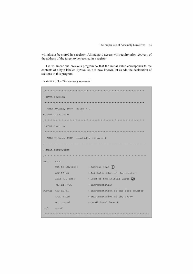
Let us amend the previous program so that the initial value corresponds to thecontents of a byte labeled Bytinit. As it is now known, let us add the declaration ofsections to this program.
EXAMPLE 3.3.– The memory operand
;****************************************************************
; DATA Section
;****************************************************************
AREA MyData, DATA, align = 2
Bytinit DCB 0x124
;****************************************************************
; CODE Section
;****************************************************************
AREA MyCode, CODE, readonly, align = 3
;– – – – – – – – – – – – – – – – – – – – – – – – – – – – – – – – –
; main subroutine
;– – – – – – – – – – – – – – – – – – – – – – – – – – – – – – – – –
main PROC
LDR R6,=Bytinit ; Address load
MOV R0,#0 ; Initialization of the counter
LDRB R3, [R6] ; Load of the initial value
MOV R4, #35 ; Incrementation
Turnal ADD R0,#1 ; Incrementation of the loop counter
ADDS R3,R4 ; Incrementation of the value
BCC Turnal ; Conditional branch
Inf B Inf
;*******************************************************************
34 Assembly Language Programming
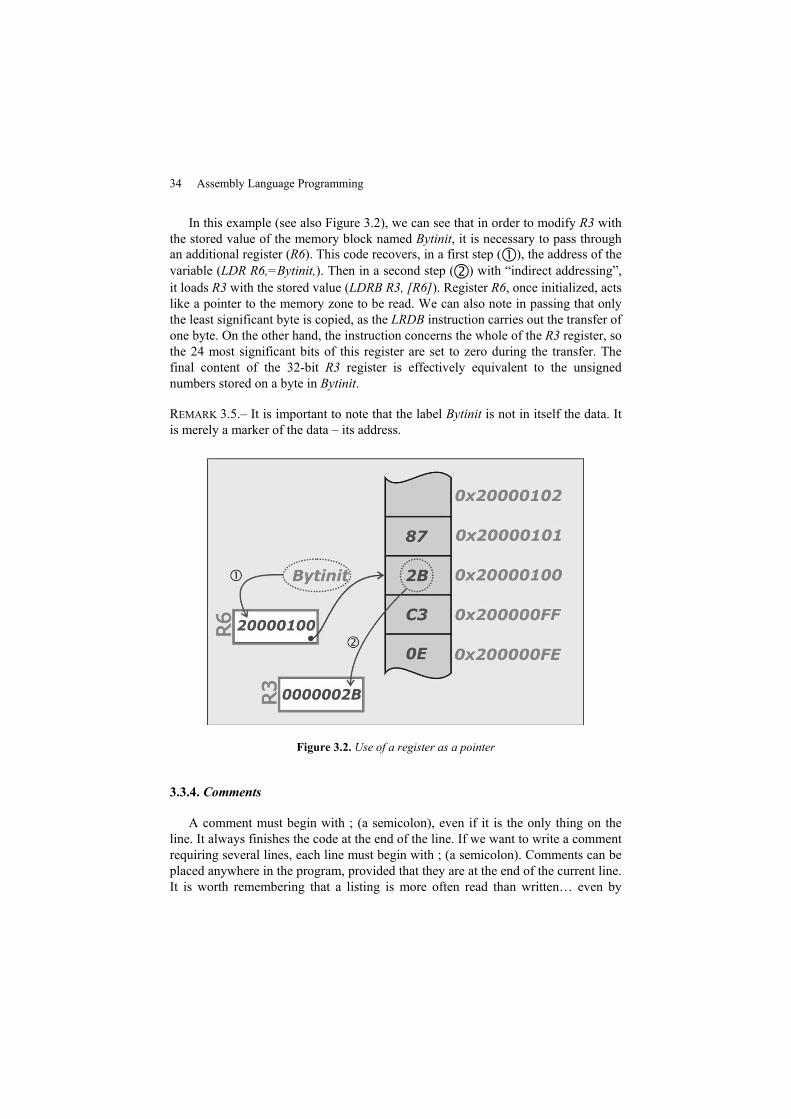
In this example (see also Figure 3.2), we can see that in order to modify R3 withthe stored value of the memory block named Bytinit, it is necessary to pass throughan additional register (R6). This code recovers, in a first step ( ), the address of thevariable (LDR R6,=Bytinit,). Then in a second step ( ) with “indirect addressing”,it loads R3 with the stored value (LDRB R3, [R6]). Register R6, once initialized, actslike a pointer to the memory zone to be read. We can also note in passing that onlythe least significant byte is copied, as the LRDB instruction carries out the transfer ofone byte. On the other hand, the instruction concerns the whole of the R3 register, sothe 24 most significant bits of this register are set to zero during the transfer. Thefinal content of the 32-bit R3 register is effectively equivalent to the unsignednumbers stored on a byte in Bytinit.
REMARK 3.5.– It is important to note that the label Bytinit is not in itself the data. Itis merely a marker of the data – its address.
Figure 3.2. Use of a register as a pointer
3.3.4. Comments
A comment must begin with ; (a semicolon), even if it is the only thing on theline. It always finishes the code at the end of the line. If we want to write a commentrequiring several lines, each line must begin with ; (a semicolon). Comments can beplaced anywhere in the program, provided that they are at the end of the current line.It is worth remembering that a listing is more often read than written… even by
The Proper use of Assembly Directives 35
those who wrote it. It is thus particularly useful when revisiting code written severalweeks, months, years, etc., earlier for it to have comments, so do not hesitate toprovide them!
3.3.5. Procedure
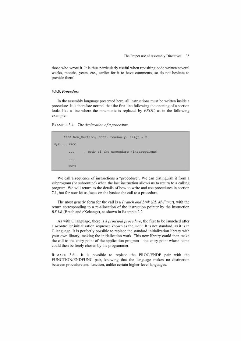
In the assembly language presented here, all instructions must be written inside aprocedure. It is therefore normal that the first line following the opening of a sectionlooks like a line where the mnemonic is replaced by PROC, as in the followingexample.
EXAMPLE 3.4.– The declaration of a procedure
AREA New_Section, CODE, readonly, align = 2
MyFunct PROC
... ; body of the procedure (instructions)
...
ENDP
We call a sequence of instructions a “procedure”. We can distinguish it from asubprogram (or subroutine) when the last instruction allows us to return to a callingprogram. We will return to the details of how to write and use procedures in section7.1, but for now let us focus on the basics: the call to a procedure.
The most generic form for the call is a Branch and Link (BL MyFunct), with thereturn corresponding to a re-allocation of the instruction pointer by the instructionBX LR (Brach and eXchange), as shown in Example 2.2.
As with C language, there is a principal procedure, the first to be launched aftera μcontroller initialization sequence known as the main. It is not standard, as it is inC language. It is perfectly possible to replace the standard initialization library withyour own library, making the initialization work. This new library could then makethe call to the entry point of the application program – the entry point whose namecould then be freely chosen by the programmer.
REMARK 3.6.– It is possible to replace the PROC/ENDP pair with theFUNCTION/ENDFUNC pair, knowing that the language makes no distinctionbetween procedure and function, unlike certain higher-level languages.
36 Assembly Language Programming
3.4. The data section
A set of directives allows us to reserve memory space that will be used by theprogram to store data. It is also possible assign such space an initial value, if needed.This manipulation seems simple but it needs to be looked at more closely.
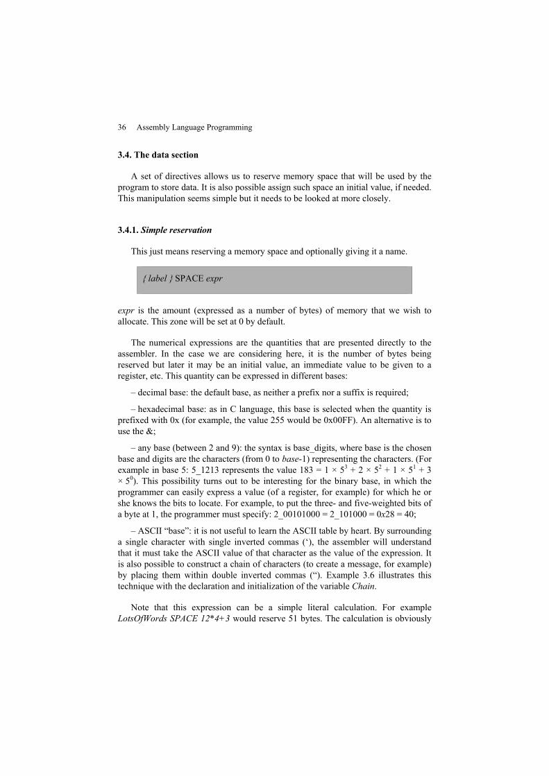
3.4.1. Simple reservation
This just means reserving a memory space and optionally giving it a name.
{ label } SPACE expr
expr is the amount (expressed as a number of bytes) of memory that we wish toallocate. This zone will be set at 0 by default.
The numerical expressions are the quantities that are presented directly to theassembler. In the case we are considering here, it is the number of bytes beingreserved but later it may be an initial value, an immediate value to be given to aregister, etc. This quantity can be expressed in different bases:
– decimal base: the default base, as neither a prefix nor a suffix is required;
– hexadecimal base: as in C language, this base is selected when the quantity isprefixed with 0x (for example, the value 255 would be 0x00FF). An alternative is touse the &;
– any base (between 2 and 9): the syntax is base_digits, where base is the chosenbase and digits are the characters (from 0 to base-1) representing the characters. (Forexample in base 5: 5_1213 represents the value 183 = 1 × 53 + 2 × 52 + 1 × 51 + 3× 50). This possibility turns out to be interesting for the binary base, in which theprogrammer can easily express a value (of a register, for example) for which he orshe knows the bits to locate. For example, to put the three- and five-weighted bits ofa byte at 1, the programmer must specify: 2_00101000 = 2_101000 = 0x28 = 40;
– ASCII “base”: it is not useful to learn the ASCII table by heart. By surroundinga single character with single inverted commas (‘), the assembler will understandthat it must take the ASCII value of that character as the value of the expression. Itis also possible to construct a chain of characters (to create a message, for example)by placing them within double inverted commas (“). Example 3.6 illustrates thistechnique with the declaration and initialization of the variable Chain.
Note that this expression can be a simple literal calculation. For exampleLotsOfWords SPACE 12*4+3 would reserve 51 bytes. The calculation is obviously
The Proper use of Assembly Directives 37
done by the assembler (and so the processor of the development host computer)when generating the code (and not at any time by Cortex-M3!). The principalarithmetic operators (+, -, *, /, >> (right shift), << (left shift), & (and), | (or), etc.)allow us to construct these literal expressions. The advanced user will find anexhaustive and detailed list of existing operators and their precedence level (relativepriority), knowing that brackets are allowed, in the technical documentation[ARM 10].
3.4.2. Reservation with initialization
Different directives exist to create memory zones containing specific values(initialized variables). Below is the list with the possible arguments:
{ label1 } FILL expr {,value{,valuesize} }
{ label2 } DCB expr1 {,expr2}{,expr2}…
{ label3 } DCD{U} expr1 {,expr2}{,expr3}…
{ label4 } DCW{U} expr1 {,expr2}{,expr3}…
{ label5 } DCQ{U} expr1 {,expr2}{,expr3}…
The reservation for FILL is the counterpart of the directive SPACE but withinitialization. We specify that we want to reserve expr initialized bytes with thevalue value, which is coded on valuesize bytes. For it to be completely consistent,the size of the reservation (expr) must be a multiple of the value of valuesize.
REMARK 3.7.– All unsigned values can be stored in a larger format than that whichis strictly necessary for their size; just add 0 in front of the useful bits. Theassembler cannot know a priori in what size it must code the information.
The other four directives specify the size of the variable with the last letter of themnemonic: B = byte, W = half-word (2 bytes), D = word (four bytes) andQ = double word (8 bytes). The data are aligned by default: a type W datum startson an even address (least significant bit at 0), and type D and Q data are on modulo4 addresses (the two least significant bits at 0).
The number of reservations therefore corresponds to a number of given initialvalues. The first initialization is compulsory. Any following this are optional. Thefollowing example uses these different directives with different bases and several
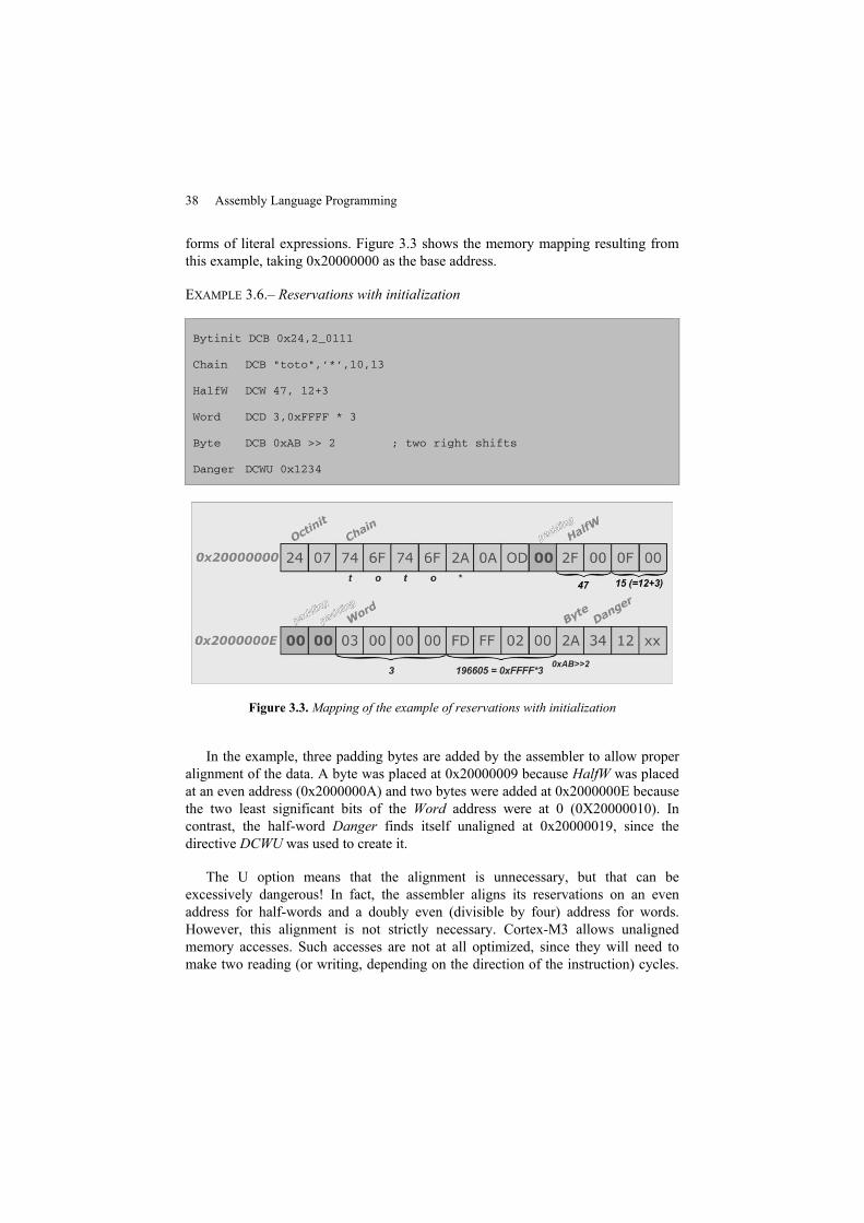
38 Assembly Language Programming
forms of literal expressions. Figure 3.3 shows the memory mapping resulting fromthis example, taking 0x20000000 as the base address.
EXAMPLE 3.6.– Reservations with initialization
Bytinit DCB 0x24,2_0111
Chain DCB "toto",’*’,10,13
HalfW DCW 47, 12+3
Word DCD 3,0xFFFF * 3
Byte DCB 0xAB >> 2 ; two right shifts
Danger DCWU 0x1234
Figure 3.3. Mapping of the example of reservations with initialization
In the example, three padding bytes are added by the assembler to allow properalignment of the data. A byte was placed at 0x20000009 because HalfW was placedat an even address (0x2000000A) and two bytes were added at 0x2000000E becausethe two least significant bits of the Word address were at 0 (0X20000010). Incontrast, the half-word Danger finds itself unaligned at 0x20000019, since thedirective DCWU was used to create it.
The U option means that the alignment is unnecessary, but that can beexcessively dangerous! In fact, the assembler aligns its reservations on an evenaddress for half-words and a doubly even (divisible by four) address for words.However, this alignment is not strictly necessary. Cortex-M3 allows unalignedmemory accesses. Such accesses are not at all optimized, since they will need tomake two reading (or writing, depending on the direction of the instruction) cycles.
The Proper use of Assembly Directives 39
It is primarily for the sake of optimality that alignment is in force at the level ofmemory reservations by the assembler. However, ARM has provided the option toprohibit unaligned access, physically speaking. This is done by setting the weightthree bit (UNALIGN_TRAP) in the Configuration Control Register to 1. Thuspositioned, any access to a half-word on an odd address, or a word at a non-doublyeven address, would cause a usage fault (see section 8.2.1.4). If your processor isconfigured in this state, it becomes essential to manage it rigorously (notably,regarding the alignment of its pointers).
3.4.3. Data initialization: the devil is in the details
What happens in the life of an initialized variable? In a normal developmentcycle, we can imagine that this variable is born in the loading of the program tomemory. The loader (program in charge of the transfer from the developmenttoolchain to the target containing Cortex-M3) will write the planned initial value tothe memory address corresponding to this variable. Then, if the variable is“variable”, it will change and no longer be equal to its initial value. Let us nowsuppose that the user restarts the target (RESET). The program restarts without goingthrough the loader step. What guarantees that the initial value will be re-transcribed?A priori in assembly language, nothing; however, it turns out that in the majority ofcases (because it is often paired with a C compiler) the assembler has anticipatedthis. The mechanism put in place is based on a doubling of initialization zones: afirst random access memory (RAM)-type address space for the variables themselvesand a duplicate in read-only memory (ROM)-type (usually just after the code)containing the initial values. It is then enough to have a routine at its disposal thatrecovers the tables of different zone addresses and then operates a copy of one overthe other. A slight adaptation of this method also allows us to reinitialize thevariables at zero. These maneuvers, although very useful, may not appear veryclearly. So in the case of the ARM-MDK (Microcontroller Development Kit), this isdone through the use of a dynamic library in the code, which is accomplished byadding a nice but nevertheless obscure IMPORT||Lib$$ Request$$armlib|| to themain file header. This initialization mechanism is revisited in detail in Chapter 9.
3.5. Is that all?
Obviously not. There are also certain directives for the assembler that are notcompletely explained in this chapter. Some of them (EQU, RN and LTORG) arediscussed in the next chapter as they deal mainly with data manipulation (and thusoperand management). Others concern the sharing (IMPORT, EXPORT) of variablesor procedures, which is the subject of Chapter 9. Yet others will not be mentionedhere because interest in their use is somewhat limited (INFO, TTL, etc.).
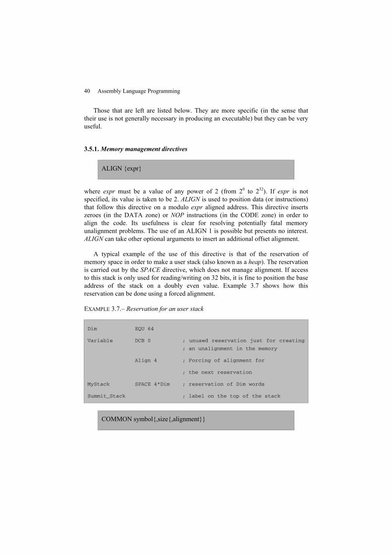
40 Assembly Language Programming
Those that are left are listed below. They are more specific (in the sense thattheir use is not generally necessary in producing an executable) but they can be veryuseful.
3.5.1.Memory management directives
ALIGN {expr}
where expr must be a value of any power of 2 (from 20 to 232). If expr is notspecified, its value is taken to be 2. ALIGN is used to position data (or instructions)that follow this directive on a modulo expr aligned address. This directive insertszeroes (in the DATA zone) or NOP instructions (in the CODE zone) in order toalign the code. Its usefulness is clear for resolving potentially fatal memoryunalignment problems. The use of an ALIGN 1 is possible but presents no interest.ALIGN can take other optional arguments to insert an additional offset alignment.
A typical example of the use of this directive is that of the reservation ofmemory space in order to make a user stack (also known as a heap). The reservationis carried out by the SPACE directive, which does not manage alignment. If accessto this stack is only used for reading/writing on 32 bits, it is fine to position the baseaddress of the stack on a doubly even value. Example 3.7 shows how thisreservation can be done using a forced alignment.
EXAMPLE 3.7.– Reservation for an user stack
Dim EQU 64
Variable DCB 0 ; unused reservation just for creating
; an unalignment in the memory
Align 4 ; Forcing of alignment for
; the next reservation
MyStack SPACE 4*Dim ; reservation of Dim words
Summit_Stack ; label on the top of the stack
COMMON symbol{,size{,alignment}}
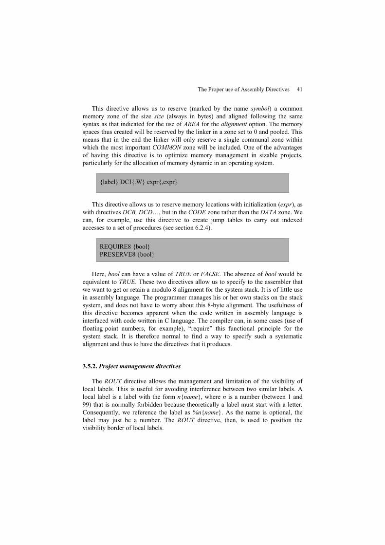
The Proper use of Assembly Directives 41
This directive allows us to reserve (marked by the name symbol) a commonmemory zone of the size size (always in bytes) and aligned following the samesyntax as that indicated for the use of AREA for the alignment option. The memoryspaces thus created will be reserved by the linker in a zone set to 0 and pooled. Thismeans that in the end the linker will only reserve a single communal zone withinwhich the most important COMMON zone will be included. One of the advantagesof having this directive is to optimize memory management in sizable projects,particularly for the allocation of memory dynamic in an operating system.
{label} DCI{.W} expr{,expr}
This directive allows us to reserve memory locations with initialization (expr), aswith directives DCB, DCD…, but in the CODE zone rather than the DATA zone. Wecan, for example, use this directive to create jump tables to carry out indexedaccesses to a set of procedures (see section 6.2.4).
REQUIRE8 {bool}PRESERVE8 {bool}
Here, bool can have a value of TRUE or FALSE. The absence of bool would beequivalent to TRUE. These two directives allow us to specify to the assembler thatwe want to get or retain a modulo 8 alignment for the system stack. It is of little usein assembly language. The programmer manages his or her own stacks on the stacksystem, and does not have to worry about this 8-byte alignment. The usefulness ofthis directive becomes apparent when the code written in assembly language isinterfaced with code written in C language. The compiler can, in some cases (use offloating-point numbers, for example), “require” this functional principle for thesystem stack. It is therefore normal to find a way to specify such a systematicalignment and thus to have the directives that it produces.
3.5.2. Project management directives
The ROUT directive allows the management and limitation of the visibility oflocal labels. This is useful for avoiding interference between two similar labels. Alocal label is a label with the form n{name}, where n is a number (between 1 and99) that is normally forbidden because theoretically a label must start with a letter.Consequently, we reference the label as %n{name}. As the name is optional, thelabel may just be a number. The ROUT directive, then, is used to position thevisibility border of local labels.
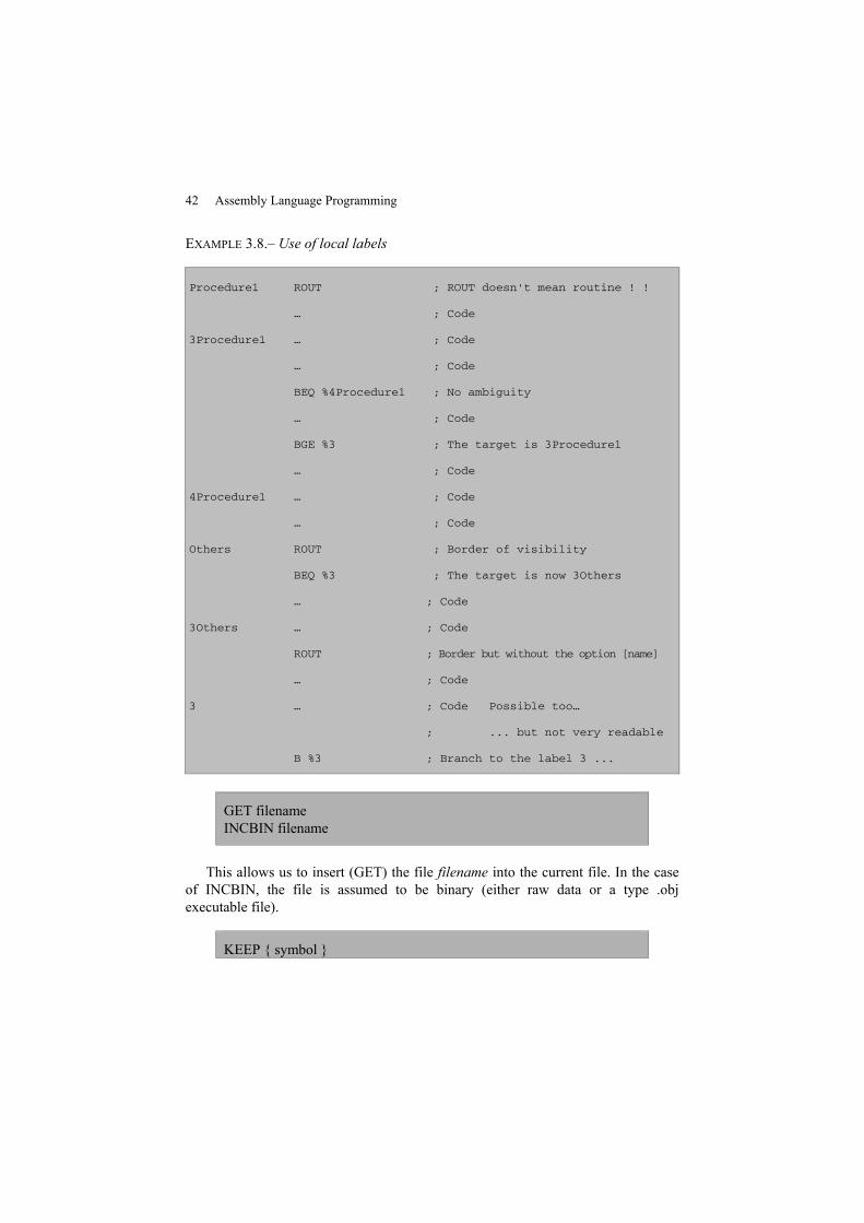
42 Assembly Language Programming
EXAMPLE 3.8.– Use of local labels
Procedure1 ROUT ; ROUT doesn't mean routine ! !
… ; Code
3Procedure1 … ; Code
… ; Code
BEQ %4Procedure1 ; No ambiguity
… ; Code
BGE %3 ; The target is 3Procedure1
… ; Code
4Procedure1 … ; Code
… ; Code
Others ROUT ; Border of visibility
BEQ %3 ; The target is now 3Others
… ; Code
3Others … ; Code
ROUT ; Border but without the option [name]
… ; Code
3 … ; Code Possible too…
; ... but not very readable
B %3 ; Branch to the label 3 ...
GET filenameINCBIN filename
This allows us to insert (GET) the file filename into the current file. In the caseof INCBIN, the file is assumed to be binary (either raw data or a type .objexecutable file).
KEEP { symbol }
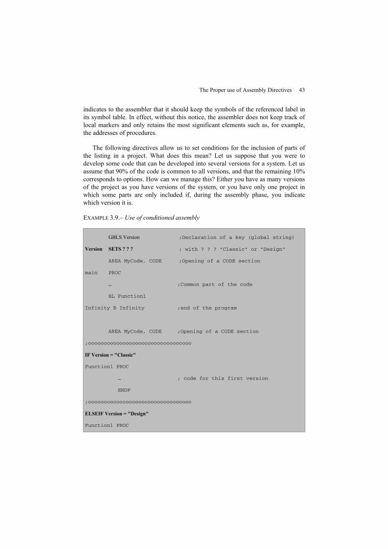
The Proper use of Assembly Directives 43
indicates to the assembler that it should keep the symbols of the referenced label inits symbol table. In effect, without this notice, the assembler does not keep track oflocal markers and only retains the most significant elements such as, for example,the addresses of procedures.
The following directives allow us to set conditions for the inclusion of parts ofthe listing in a project. What does this mean? Let us suppose that you were todevelop some code that can be developed into several versions for a system. Let usassume that 90% of the code is common to all versions, and that the remaining 10%corresponds to options. How can we manage this? Either you have as many versionsof the project as you have versions of the system, or you have only one project inwhich some parts are only included if, during the assembly phase, you indicatewhich version it is.
EXAMPLE 3.9.– Use of conditioned assembly
GBLS Version ;Declaration of a key (global string)
Version SETS ? ? ? ; with ? ? ? "Classic" or "Design"
AREA MyCode, CODE ;Opening of a CODE section
main PROC
… ;Common part of the code
BL Function1
Infinity B Infinity ;end of the program
AREA MyCode, CODE ;Opening of a CODE section
;ooooooooooooooooooooooooooooooooo
IF Version = "Classic"
Function1 PROC
… ; code for this first version
ENDP
;ooooooooooooooooooooooooooooooooo
ELSEIF Version = "Design"
Function1 PROC
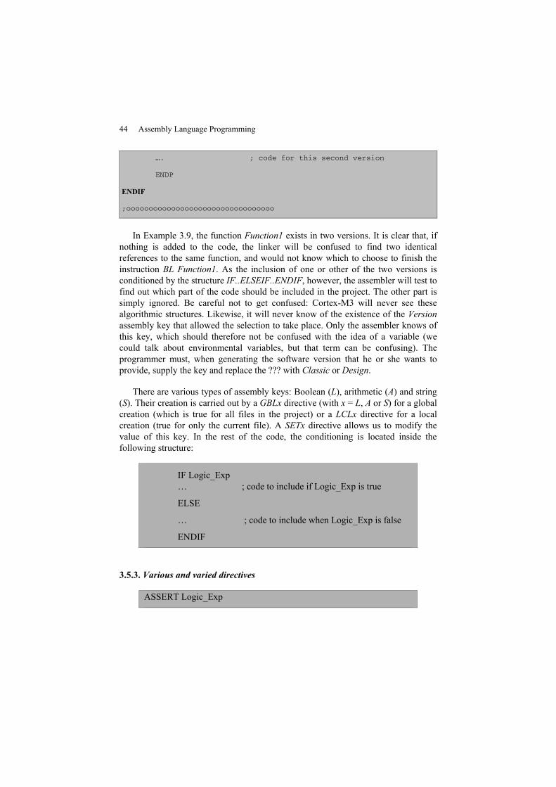
44 Assembly Language Programming
…. ; code for this second version
ENDP
ENDIF
;ooooooooooooooooooooooooooooooooo
In Example 3.9, the function Function1 exists in two versions. It is clear that, ifnothing is added to the code, the linker will be confused to find two identicalreferences to the same function, and would not know which to choose to finish theinstruction BL Function1. As the inclusion of one or other of the two versions isconditioned by the structure IF..ELSEIF..ENDIF, however, the assembler will test tofind out which part of the code should be included in the project. The other part issimply ignored. Be careful not to get confused: Cortex-M3 will never see thesealgorithmic structures. Likewise, it will never know of the existence of the Versionassembly key that allowed the selection to take place. Only the assembler knows ofthis key, which should therefore not be confused with the idea of a variable (wecould talk about environmental variables, but that term can be confusing). Theprogrammer must, when generating the software version that he or she wants toprovide, supply the key and replace the ??? with Classic or Design.
There are various types of assembly keys: Boolean (L), arithmetic (A) and string(S). Their creation is carried out by a GBLx directive (with x = L, A or S) for a globalcreation (which is true for all files in the project) or a LCLx directive for a localcreation (true for only the current file). A SETx directive allows us to modify thevalue of this key. In the rest of the code, the conditioning is located inside thefollowing structure:
IF Logic_Exp… ; code to include if Logic_Exp is true
ELSE
… ; code to include when Logic_Exp is false
ENDIF
3.5.3. Various and varied directives
ASSERT Logic_Exp
The Proper use of Assembly Directives 45
The above directive allows us to display a message (such as an error message)during the second assembly phase (an assembler takes several passes to carry out itswork). If Logic_Exp is false:
name CN expr
allows us to rename a register in a possible coprocessor:
{ label } DCFSU fpliteral{,fpliteral}…
which allows us to reserve initialized memory space for floating points. This impliesthat the program has access to floating-point calculation libraries and/or that afloating-point arithmetic unit type coprocessor is attached to the Cortex-M3structure.
ENTRY
The above defines the entry point of the program. This directive is essential ifyou create all of the code. If you use a processor initialization library, it willintegrate entry point management. In this case, you should avoid using this directive.
IMPORT EXPORT
The two directives above allow us to share a symbol (name of a procedure, of avariable, etc.) between several files of a single project. Their advantages and useswill be elaborated on in section 9.1.5.

Chapter 4
Operands of Instructions
Chapter 3 showed us how a program written in assembly language is formed. Letus now look at techniques in this language for accessing and manipulating data. Thisinvolves defining what an operand is. First, let us specify that this processor has aload/store type structure. It is therefore only possible to access memory zones in theData section by using specific instructions. For these instructions, one of theoperands will necessarily be the address of a memory location where it will need toread or write. The way to describe this address corresponds to the term addressingmode and will be covered at the end of this chapter.
For other instructions, the operands are explicitly given values (immediateoperand), contents of registers, or labels in the case of branch instructions. In orderto specify which operands a programmer wants to use to carry out the operation, heor she writes an expression made up of numbers and symbols.
When the instruction takes two or three operands, as in the following example:
Instr op1,o2{,op3}
op1 is called the destination operand. It is this operand that receives the result of theoperation or assignment. Operands op2 and op3 are called source operands, as theyserve to supply the instruction.
REMARK 4.1.– For read (LDR (LoaD Register), etc.) and write (STR (SToreRegister), etc) instructions (see section 5.7), the meanings of destination and sourceoperands are reversed. This is a source of error when writing a source program inassembly language, even if at the instruction level we can see a certain logic.
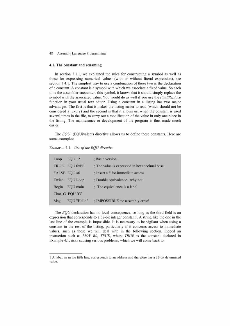
48 Assembly Language Programming
4.1. The constant and renaming
In section 3.1.1, we explained the rules for constructing a symbol as well asthose for expressing numerical values (with or without literal expression), seesection 3.4.1. The simplest way to use a combination of these two is the declarationof a constant. A constant is a symbol with which we associate a fixed value. So eachtime the assembler encounters this symbol, it knows that it should simply replace thesymbol with the associated value. You would do as well if you use the Find/Replacefunction in your usual text editor. Using a constant in a listing has two majoradvantages. The first is that it makes the listing easier to read (which should not beconsidered a luxury) and the second is that it allows us, when the constant is usedseveral times in the file, to carry out a modification of the value in only one place inthe listing. The maintenance or development of the program is thus made mucheasier.
The EQU (EQUivalent) directive allows us to define these constants. Here aresome examples:
EXAMPLE 4.1.– Use of the EQU directive
Loop EQU 12 ; Basic version
TRUE EQU 0xFF ; The value is expressed in hexadecimal base
FALSE EQU #0 ; Insert a # for immediate access
Twice EQU Loop ; Double equivalence...why not!
Begin EQU main ; The equivalence is a label
Char_G EQU ’G’
Msg EQU "Hello" ; IMPOSSIBLE => assembly error!
The EQU declaration has no local consequence, so long as the third field is anexpression that corresponds to a 32-bit integer constant1. A string like the one in thelast line of the example is impossible. It is necessary to be vigilant when using aconstant in the rest of the listing, particularly if it concerns access to immediatevalues, such as those we will deal with in the following section. Indeed aninstruction such as MOV R0, TRUE, where TRUE is the constant declared inExample 4.1, risks causing serious problems, which we will come back to.
1 A label, as in the fifth line, corresponds to an address and therefore has a 32-bit determinedvalue.
Operands of Instructions 49
The directive RN (ReName) can also make the listing more readable (although):
name RN n
where n is a number between 0 and 15 and serves to identify the general register thatis the target of this directive. The directive allows us to rename the target registerwith a proposed name. So Counter RN 0 allows us to use the symbol Counterinstead of the symbol R0 in the rest of the listing. This makes sense even if, in theend, the disappearance of the name of a general register in the listing can confuse aprogrammer. You can also definitively discourage future readers by writing XV34_ZRN 1 and R_4 RN 2. Register R2 would become R_4 and register R1 would becomeXV34_Z. In terms of readability, this does not seem like an improvement2!
4.2. Operands for common instructions
By common instructions, we mean the set of instructions other than theread/write instructions.
4.2.1. Use of registers
4.2.1.1. General registers
In most instructions (and the examples presented here follow this approach), theprogrammer will mainly use the general registers R0 to R12 to store the values withwhich he or she carries out the common instructions. As such, the registers could beconsidered local variables. General registers are thus the most common operandsthat we come across in a program. They can contain quantities that express values ofvery different natures (an 8-bit integer for the ASCII code of a character, anunsigned 16-bit integer for an array index, a signed integer for a relativedisplacement in the program, etc.). Whatever the case, the 13 registers will alwaysbe seen by the processor as a quantity coded on 32 bits. The programmer is facedwith mastering the entire contents of a register when the information that he or she isdealing with only holds a half or a quarter of it.
From the coding point of view, it can be interesting to see what the codegenerated by the assembler looks like. Let us take the simple addition instructionADD R0,R1 as an example. This adds together the value contained in the tworegisters and stores the result in R0. This result is a priori of the Thumb type. Itscoding (and so what will be stored in the CODE memory) is on 16 bits and its
2 Not all registers are allowed! For example, R3 RN 4 is impossible.
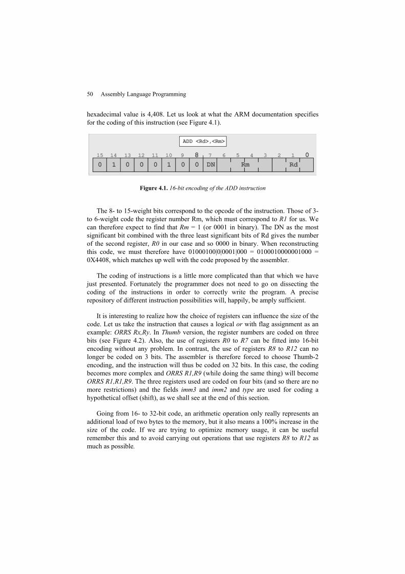
50 Assembly Language Programming
hexadecimal value is 4,408. Let us look at what the ARM documentation specifiesfor the coding of this instruction (see Figure 4.1).
Figure 4.1. 16-bit encoding of the ADD instruction
The 8- to 15-weight bits correspond to the opcode of the instruction. Those of 3-to 6-weight code the register number Rm, which must correspond to R1 for us. Wecan therefore expect to find that Rm = 1 (or 0001 in binary). The DN as the mostsignificant bit combined with the three least significant bits of Rd gives the numberof the second register, R0 in our case and so 0000 in binary. When reconstructingthis code, we must therefore have 01000100|0|0001|000 = 0100010000001000 =0X4408, which matches up well with the code proposed by the assembler.
The coding of instructions is a little more complicated than that which we havejust presented. Fortunately the programmer does not need to go on dissecting thecoding of the instructions in order to correctly write the program. A preciserepository of different instruction possibilities will, happily, be amply sufficient.
It is interesting to realize how the choice of registers can influence the size of thecode. Let us take the instruction that causes a logical or with flag assignment as anexample: ORRS Rx,Ry. In Thumb version, the register numbers are coded on threebits (see Figure 4.2). Also, the use of registers R0 to R7 can be fitted into 16-bitencoding without any problem. In contrast, the use of registers R8 to R12 can nolonger be coded on 3 bits. The assembler is therefore forced to choose Thumb-2encoding, and the instruction will thus be coded on 32 bits. In this case, the codingbecomes more complex and ORRS R1,R9 (while doing the same thing) will becomeORRS R1,R1,R9. The three registers used are coded on four bits (and so there are nomore restrictions) and the fields imm3 and imm2 and type are used for coding ahypothetical offset (shift), as we shall see at the end of this section.
Going from 16- to 32-bit code, an arithmetic operation only really represents anadditional load of two bytes to the memory, but it also means a 100% increase in thesize of the code. If we are trying to optimize memory usage, it can be usefulremember this and to avoid carrying out operations that use registers R8 to R12 asmuch as possible.
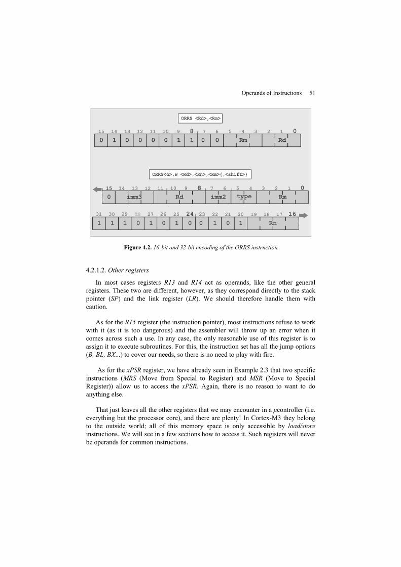
Operands of Instructions 51
Figure 4.2. 16-bit and 32-bit encoding of the ORRS instruction
4.2.1.2. Other registers
In most cases registers R13 and R14 act as operands, like the other generalregisters. These two are different, however, as they correspond directly to the stackpointer (SP) and the link register (LR). We should therefore handle them withcaution.
As for the R15 register (the instruction pointer), most instructions refuse to workwith it (as it is too dangerous) and the assembler will throw up an error when itcomes across such a use. In any case, the only reasonable use of this register is toassign it to execute subroutines. For this, the instruction set has all the jump options(B, BL, BX...) to cover our needs, so there is no need to play with fire.
As for the xPSR register, we have already seen in Example 2.3 that two specificinstructions (MRS (Move from Special to Register) and MSR (Move to SpecialRegister)) allow us to access the xPSR. Again, there is no reason to want to doanything else.
That just leaves all the other registers that we may encounter in a μcontroller (i.e.everything but the processor core), and there are plenty! In Cortex-M3 they belongto the outside world; all of this memory space is only accessible by load/storeinstructions. We will see in a few sections how to access it. Such registers will neverbe operands for common instructions.
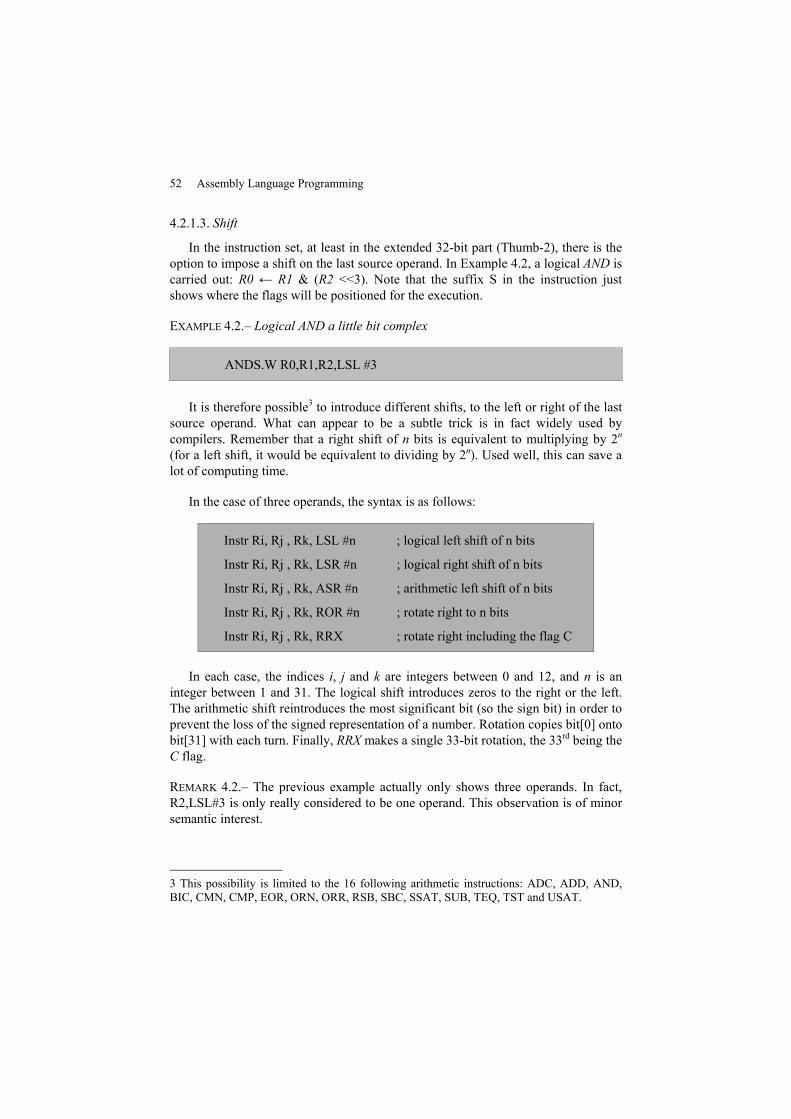
52 Assembly Language Programming
4.2.1.3. Shift
In the instruction set, at least in the extended 32-bit part (Thumb-2), there is theoption to impose a shift on the last source operand. In Example 4.2, a logical AND iscarried out: R0 ← R1 & (R2 <<3). Note that the suffix S in the instruction justshows where the flags will be positioned for the execution.
EXAMPLE 4.2.– Logical AND a little bit complex
ANDS.W R0,R1,R2,LSL #3
It is therefore possible3 to introduce different shifts, to the left or right of the lastsource operand. What can appear to be a subtle trick is in fact widely used bycompilers. Remember that a right shift of n bits is equivalent to multiplying by 2n
(for a left shift, it would be equivalent to dividing by 2n). Used well, this can save alot of computing time.
In the case of three operands, the syntax is as follows:
Instr Ri, Rj , Rk, LSL #n ; logical left shift of n bits
Instr Ri, Rj , Rk, LSR #n ; logical right shift of n bits
Instr Ri, Rj , Rk, ASR #n ; arithmetic left shift of n bits
Instr Ri, Rj , Rk, ROR #n ; rotate right to n bits
Instr Ri, Rj , Rk, RRX ; rotate right including the flag C
In each case, the indices i, j and k are integers between 0 and 12, and n is aninteger between 1 and 31. The logical shift introduces zeros to the right or the left.The arithmetic shift reintroduces the most significant bit (so the sign bit) in order toprevent the loss of the signed representation of a number. Rotation copies bit[0] ontobit[31] with each turn. Finally, RRX makes a single 33-bit rotation, the 33rd being theC flag.
REMARK 4.2.– The previous example actually only shows three operands. In fact,R2,LSL#3 is only really considered to be one operand. This observation is of minorsemantic interest.
3 This possibility is limited to the 16 following arithmetic instructions: ADC, ADD, AND,BIC, CMN, CMP, EOR, ORN, ORR, RSB, SBC, SSAT, SUB, TEQ, TST and USAT.
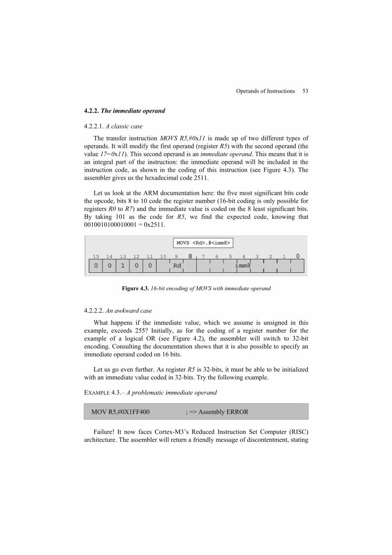
Operands of Instructions 53
4.2.2. The immediate operand
4.2.2.1. A classic case
The transfer instruction MOVS R5,#0x11 is made up of two different types ofoperands. It will modify the first operand (register R5) with the second operand (thevalue 17=0x11). This second operand is an immediate operand. This means that it isan integral part of the instruction: the immediate operand will be included in theinstruction code, as shown in the coding of this instruction (see Figure 4.3). Theassembler gives us the hexadecimal code 2511.
Let us look at the ARM documentation here: the five most significant bits codethe opcode, bits 8 to 10 code the register number (16-bit coding is only possible forregisters R0 to R7) and the immediate value is coded on the 8 least significant bits.By taking 101 as the code for R5, we find the expected code, knowing that0010010100010001 = 0x2511.
Figure 4.3. 16-bit encoding of MOVS with immediate operand
4.2.2.2. An awkward case
What happens if the immediate value, which we assume is unsigned in thisexample, exceeds 255? Initially, as for the coding of a register number for theexample of a logical OR (see Figure 4.2), the assembler will switch to 32-bitencoding. Consulting the documentation shows that it is also possible to specify animmediate operand coded on 16 bits.
Let us go even further. As register R5 is 32-bits, it must be able to be initializedwith an immediate value coded in 32-bits. Try the following example.
EXAMPLE 4.3.– A problematic immediate operand
MOV R5,#0X1FF400 ; => Assembly ERROR
Failure! It now faces Cortex-M3’s Reduced Instruction Set Computer (RISC)architecture. The assembler will return a friendly message of discontentment, stating
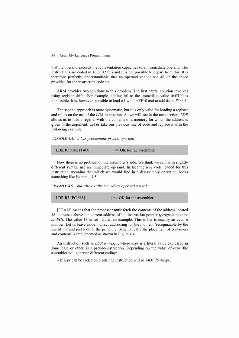
54 Assembly Language Programming
that the operand exceeds the representation capacities of an immediate operand. Theinstructions are coded in 16 or 32 bits and it is not possible to depart from this. It istherefore perfectly understandable that an operand cannot use all of the spaceprovided for the instruction code set.
ARM provides two solutions to this problem. The first partial solution involvesusing register shifts. For example, adding R0 to the immediate value 0xff100 isimpossible. It is, however, possible to load R1 with 0xFF10 and to add R0 to R1<<4.
The second approach is more systematic, but it is only valid for loading a registerand relies on the use of the LDR instruction. As we will see in the next section, LDRallows us to load a register with the contents of a memory for which the address isgiven in the argument. Let us take our previous line of code and replace it with thefollowing example.
EXAMPLE 4.4.– A less problematic pseudo-operand
LDR R5,=0x1FF400 ; => OK for the assembler
Now there is no problem on the assembler’s side. We think we can, with slightlydifferent syntax, use an immediate operand. In fact the true code loaded for thisinstruction, meaning that which we would find in a disassembly operation, lookssomething like Example 4.5.
EXAMPLE 4.5.– but where is the immediate operand passed?
LDR R5,[PC,#18] ; => OK for the assembler
[PC,#18] means that the processor must fetch the contents of the address located18 addresses above the current address of the instruction pointer (program counteror PC). The value 18 is set here as an example. This offset is usually an even nnumber. Let us leave aside indirect addressing for the moment (recognizable by theuse of []), and just look at the principle. Schematically the placement of containersand contents is implemented as shown in Figure 4.4.
An instruction such as LDR Ri =expr, where expr is a literal value expressed insome base or other, is a pseudo-instruction. Depending on the value of expr, theassembler will generate different coding:
– if expr can be coded on 8 bits, the instruction will beMOV Ri, #expr;
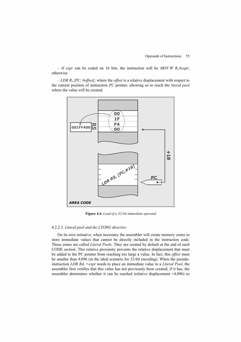
Operands of Instructions 55
– if expr can be coded on 16 bits, the instruction will be MOV.W Ri,#expr;otherwise
– LDR Ri,{PC, #offset], where the offset is a relative displacement with respect tothe current position of instruction PC pointer, allowing us to reach the literal poolwhere the value will be created.
Figure 4.4. Load of a 32-bit immediate operand
4.2.2.3. Literal pool and the LTORG directive
On its own initiative, when necessary the assembler will create memory zones tostore immediate values that cannot be directly included in the instruction code.These zones are called Literal Pools. They are created by default at the end of eachCODE section. This relative proximity prevents the relative displacement that mustbe added to the PC pointer from reaching too large a value. In fact, this offset mustbe smaller than 4,096 (in the ideal scenario for 32-bit encoding). When the pseudo-instruction LDR Rd, =expr needs to place an immediate value in a Literal Pool, theassembler first verifies that this value has not previously been created; if it has, theassembler determines whether it can be reached (relative displacement <4,096) so
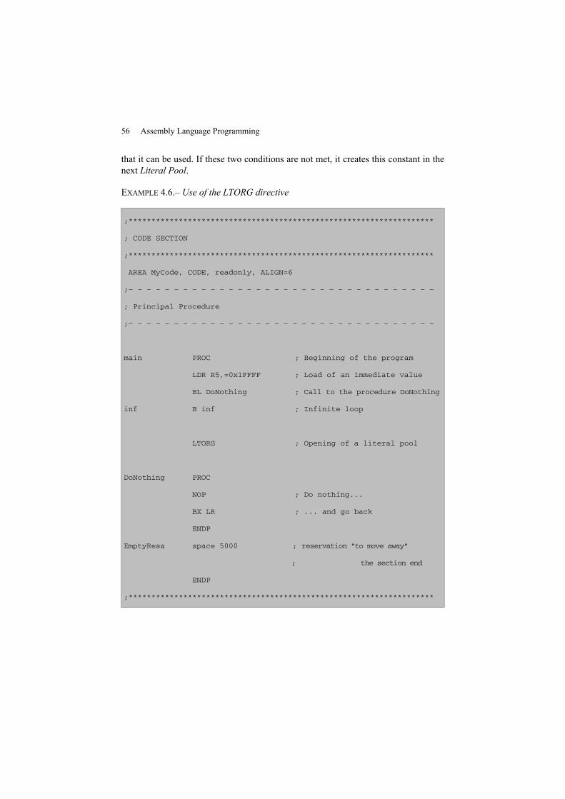
56 Assembly Language Programming
that it can be used. If these two conditions are not met, it creates this constant in thenext Literal Pool.
EXAMPLE 4.6.– Use of the LTORG directive
;*******************************************************************
; CODE SECTION
;*******************************************************************
AREA MyCode, CODE, readonly, ALIGN=6
;– – – – – – – – – – – – – – – – – – – – – – – – – – – – – – – – – –
; Principal Procedure
;– – – – – – – – – – – – – – – – – – – – – – – – – – – – – – – – – –
main PROC ; Beginning of the program
LDR R5,=0x1FFFF ; Load of an immediate value
BL DoNothing ; Call to the procedure DoNothing
inf B inf ; Infinite loop
LTORG ; Opening of a literal pool
DoNothing PROC
NOP ; Do nothing...
BX LR ; ... and go back
ENDP
EmptyResa space 5000 ; reservation “to move away”
; the section end
ENDP
;*******************************************************************
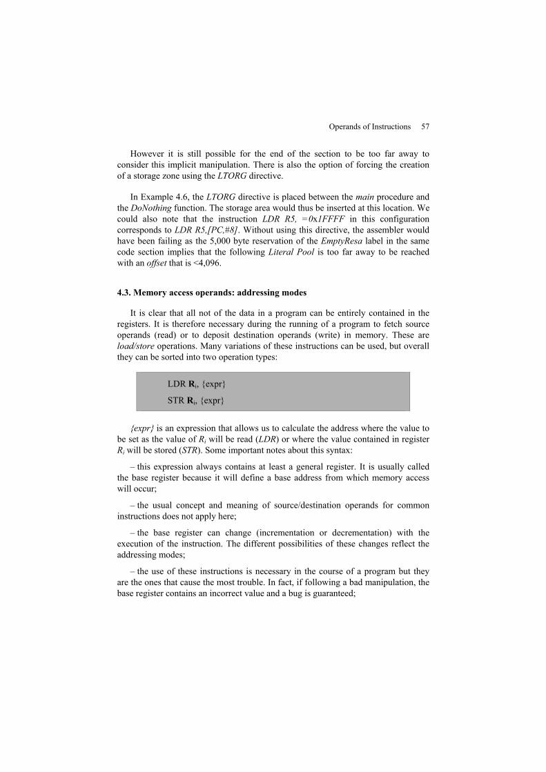
Operands of Instructions 57
However it is still possible for the end of the section to be too far away toconsider this implicit manipulation. There is also the option of forcing the creationof a storage zone using the LTORG directive.
In Example 4.6, the LTORG directive is placed between the main procedure andthe DoNothing function. The storage area would thus be inserted at this location. Wecould also note that the instruction LDR R5, =0x1FFFF in this configurationcorresponds to LDR R5,[PC,#8]. Without using this directive, the assembler wouldhave been failing as the 5,000 byte reservation of the EmptyResa label in the samecode section implies that the following Literal Pool is too far away to be reachedwith an offset that is <4,096.
4.3. Memory access operands: addressing modes
It is clear that all not of the data in a program can be entirely contained in theregisters. It is therefore necessary during the running of a program to fetch sourceoperands (read) or to deposit destination operands (write) in memory. These areload/store operations. Many variations of these instructions can be used, but overallthey can be sorted into two operation types:
LDR Ri, {expr}
STR Ri, {expr}
{expr} is an expression that allows us to calculate the address where the value tobe set as the value of Ri will be read (LDR) or where the value contained in registerRi will be stored (STR). Some important notes about this syntax:
– this expression always contains at least a general register. It is usually calledthe base register because it will define a base address from which memory accesswill occur;
– the usual concept and meaning of source/destination operands for commoninstructions does not apply here;
– the base register can change (incrementation or decrementation) with theexecution of the instruction. The different possibilities of these changes reflect theaddressing modes;
– the use of these instructions is necessary in the course of a program but theyare the ones that cause the most trouble. In fact, if following a bad manipulation, thebase register contains an incorrect value and a bug is guaranteed;
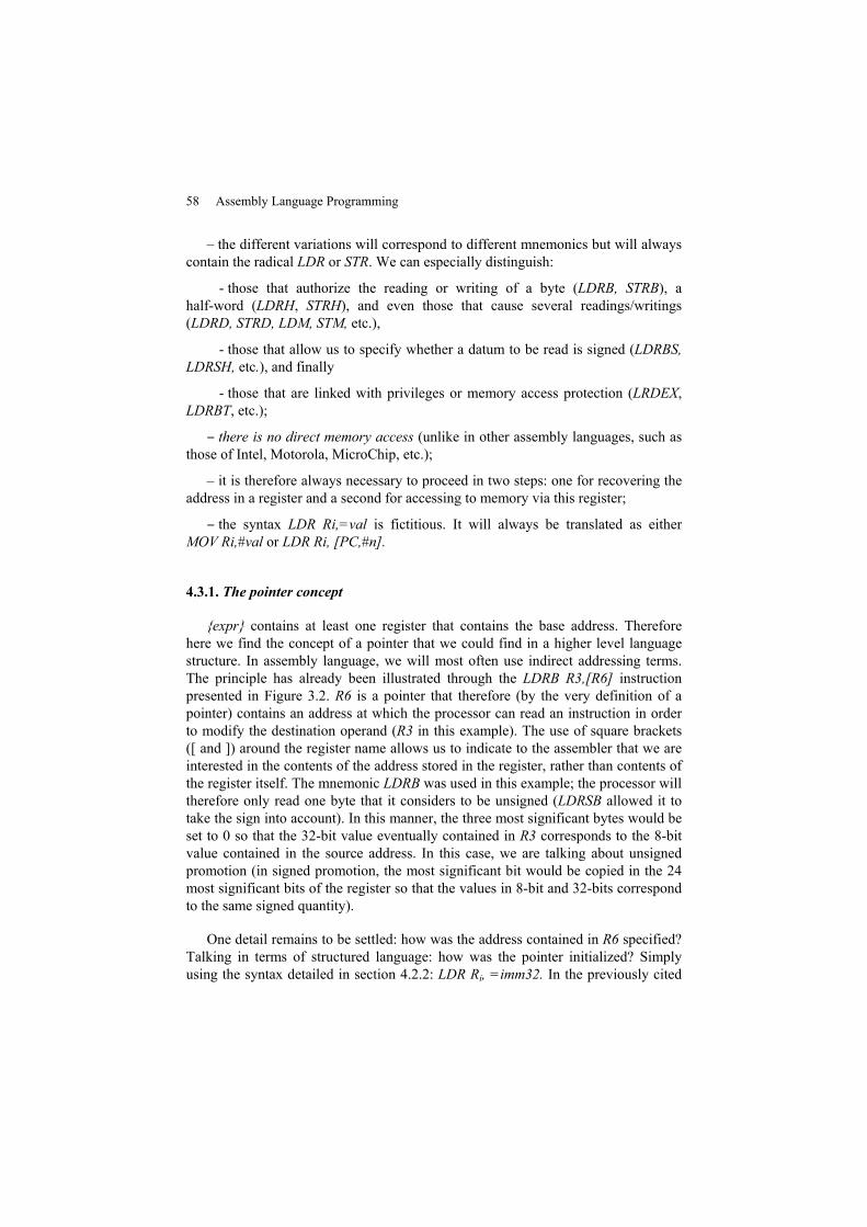
58 Assembly Language Programming
– the different variations will correspond to different mnemonics but will alwayscontain the radical LDR or STR. We can especially distinguish:
- those that authorize the reading or writing of a byte (LDRB, STRB), ahalf-word (LDRH, STRH), and even those that cause several readings/writings(LDRD, STRD, LDM, STM, etc.),
- those that allow us to specify whether a datum to be read is signed (LDRBS,LDRSH, etc.), and finally
- those that are linked with privileges or memory access protection (LRDEX,LDRBT, etc.);‒ there is no direct memory access (unlike in other assembly languages, such asthose of Intel, Motorola, MicroChip, etc.);
– it is therefore always necessary to proceed in two steps: one for recovering theaddress in a register and a second for accessing to memory via this register;‒ the syntax LDR Ri,=val is fictitious. It will always be translated as eitherMOV Ri,#val or LDR Ri, [PC,#n].
4.3.1. The pointer concept
{expr} contains at least one register that contains the base address. Thereforehere we find the concept of a pointer that we could find in a higher level languagestructure. In assembly language, we will most often use indirect addressing terms.The principle has already been illustrated through the LDRB R3,[R6] instructionpresented in Figure 3.2. R6 is a pointer that therefore (by the very definition of apointer) contains an address at which the processor can read an instruction in orderto modify the destination operand (R3 in this example). The use of square brackets([ and ]) around the register name allows us to indicate to the assembler that we areinterested in the contents of the address stored in the register, rather than contents ofthe register itself. The mnemonic LDRB was used in this example; the processor willtherefore only read one byte that it considers to be unsigned (LDRSB allowed it totake the sign into account). In this manner, the three most significant bytes would beset to 0 so that the 32-bit value eventually contained in R3 corresponds to the 8-bitvalue contained in the source address. In this case, we are talking about unsignedpromotion (in signed promotion, the most significant bit would be copied in the 24most significant bits of the register so that the values in 8-bit and 32-bits correspondto the same signed quantity).
One detail remains to be settled: how was the address contained in R6 specified?Talking in terms of structured language: how was the pointer initialized? Simplyusing the syntax detailed in section 4.2.2: LDR Ri, =imm32. In the previously cited
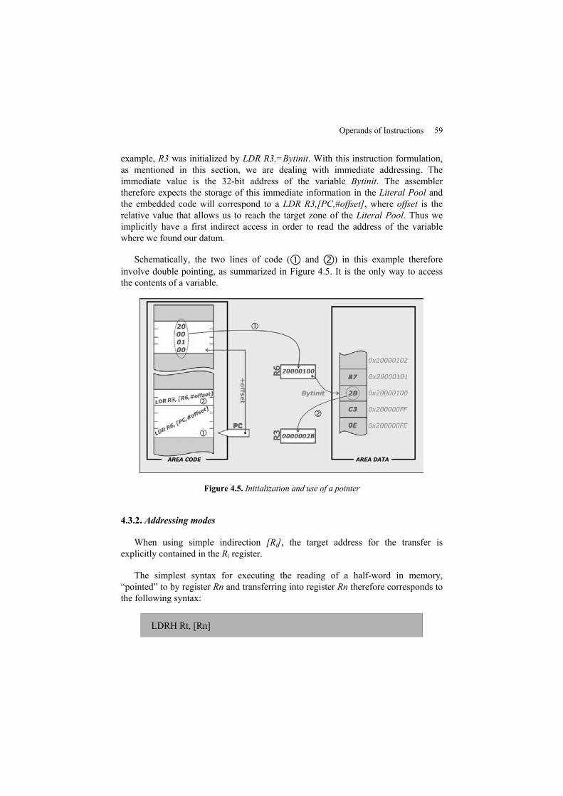
Operands of Instructions 59
example, R3 was initialized by LDR R3,=Bytinit. With this instruction formulation,as mentioned in this section, we are dealing with immediate addressing. Theimmediate value is the 32-bit address of the variable Bytinit. The assemblertherefore expects the storage of this immediate information in the Literal Pool andthe embedded code will correspond to a LDR R3,[PC,#offset], where offset is therelative value that allows us to reach the target zone of the Literal Pool. Thus weimplicitly have a first indirect access in order to read the address of the variablewhere we found our datum.
Schematically, the two lines of code ( and ) in this example thereforeinvolve double pointing, as summarized in Figure 4.5. It is the only way to accessthe contents of a variable.
Figure 4.5. Initialization and use of a pointer
4.3.2. Addressing modes
When using simple indirection [Ri], the target address for the transfer isexplicitly contained in the Ri register.
The simplest syntax for executing the reading of a half-word in memory,“pointed” to by register Rn and transferring into register Rn therefore corresponds tothe following syntax:
LDRH Rt, [Rn]
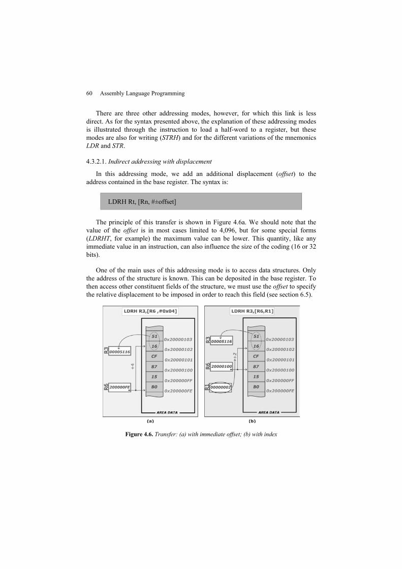
60 Assembly Language Programming
There are three other addressing modes, however, for which this link is lessdirect. As for the syntax presented above, the explanation of these addressing modesis illustrated through the instruction to load a half-word to a register, but thesemodes are also for writing (STRH) and for the different variations of the mnemonicsLDR and STR.
4.3.2.1. Indirect addressing with displacement
In this addressing mode, we add an additional displacement (offset) to theaddress contained in the base register. The syntax is:
LDRH Rt, [Rn, #±offset]
The principle of this transfer is shown in Figure 4.6a. We should note that thevalue of the offset is in most cases limited to 4,096, but for some special forms(LDRHT, for example) the maximum value can be lower. This quantity, like anyimmediate value in an instruction, can also influence the size of the coding (16 or 32bits).
One of the main uses of this addressing mode is to access data structures. Onlythe address of the structure is known. This can be deposited in the base register. Tothen access other constituent fields of the structure, we must use the offset to specifythe relative displacement to be imposed in order to reach this field (see section 6.5).
Figure 4.6. Transfer: (a) with immediate offset; (b) with index
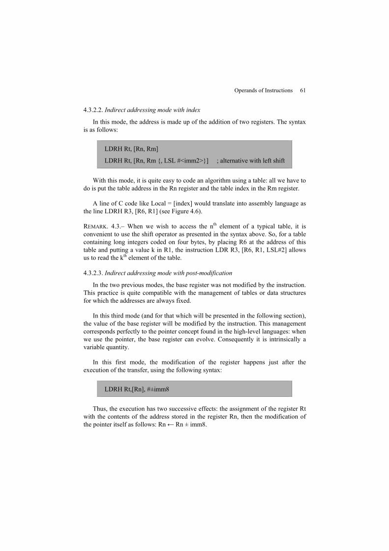
Operands of Instructions 61
4.3.2.2. Indirect addressing mode with index
In this mode, the address is made up of the addition of two registers. The syntaxis as follows:
LDRH Rt, [Rn, Rm]
LDRH Rt, [Rn, Rm {, LSL #<imm2>}] ; alternative with left shift
With this mode, it is quite easy to code an algorithm using a table: all we have todo is put the table address in the Rn register and the table index in the Rm register.
A line of C code like Local = [index] would translate into assembly language asthe line LDRH R3, [R6, R1] (see Figure 4.6).
REMARK. 4.3.– When we wish to access the nth element of a typical table, it isconvenient to use the shift operator as presented in the syntax above. So, for a tablecontaining long integers coded on four bytes, by placing R6 at the address of thistable and putting a value k in R1, the instruction LDR R3, [R6, R1, LSL#2] allowsus to read the kth element of the table.
4.3.2.3. Indirect addressing mode with post-modification
In the two previous modes, the base register was not modified by the instruction.This practice is quite compatible with the management of tables or data structuresfor which the addresses are always fixed.
In this third mode (and for that which will be presented in the following section),the value of the base register will be modified by the instruction. This managementcorresponds perfectly to the pointer concept found in the high-level languages: whenwe use the pointer, the base register can evolve. Consequently it is intrinsically avariable quantity.
In this first mode, the modification of the register happens just after theexecution of the transfer, using the following syntax:
LDRH Rt,[Rn], #±imm8
Thus, the execution has two successive effects: the assignment of the register Rtwith the contents of the address stored in the register Rn, then the modification ofthe pointer itself as follows: Rn← Rn ± imm8.
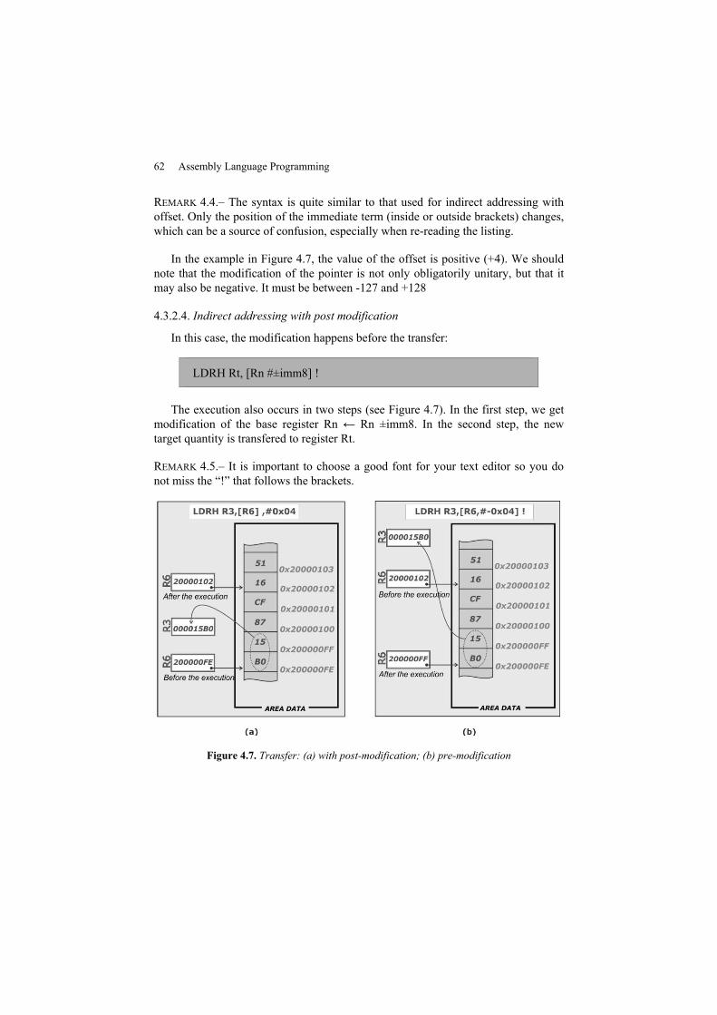
62 Assembly Language Programming
REMARK 4.4.– The syntax is quite similar to that used for indirect addressing withoffset. Only the position of the immediate term (inside or outside brackets) changes,which can be a source of confusion, especially when re-reading the listing.
In the example in Figure 4.7, the value of the offset is positive (+4). We shouldnote that the modification of the pointer is not only obligatorily unitary, but that itmay also be negative. It must be between -127 and +128
4.3.2.4. Indirect addressing with post modification
In this case, the modification happens before the transfer:
LDRH Rt, [Rn #±imm8] !
The execution also occurs in two steps (see Figure 4.7). In the first step, we getmodification of the base register Rn ← Rn ±imm8. In the second step, the newtarget quantity is transfered to register Rt.
REMARK 4.5.– It is important to choose a good font for your text editor so you donot miss the “!” that follows the brackets.
Figure 4.7. Transfer: (a) with post-modification; (b) pre-modification
Chapter 5
Instruction Set
Reading an instruction set is anything but pleasant. In their first reading of thischapter, readers will just skim through, but in the end, this is definitely the chapterthat the user will return to the most often to find out what the processor can do andabove all how he or she can make it do that (i.e. with which operands).
5.1. Reading guide
A certain number of conventions, omissions or implicit rules govern thecompilation of the explanations of the instruction set. It is therefore necessary toread these sections while taking into account the following remarks:
– some instructions are only mentioned (at the end of the chapter) and are notexplained. They are advanced instructions for the processor and so are directed atadvanced programmers who would not, in any case, be satisfied with this singlebook;
– the majority of instructions are in a 16- or 32-bit version. The assembler,according to its own implicit rules and functional limits (the size of the immediateoperands, for example) will choose one or the other. It is, however, possible to forcethe desired code size by adding the .W for a 32-bit or .N for a 16-bit extension. Indoing so, this may lead to greater mastery of the code fabrication process but at theexpense of failure in the event that it is impossible to code the instruction in the codewith the suffix <q>. In this book we will only indicate the possible sizes (16, 16/32or 32 bits) for each instruction, it being understood that forcing is only reasonable ifthe size is not fixed.

64 Assembly Language Programming
REMARK 5.1.– W means word but sometimes (like in this chapter) it means a 32-bitquantity and sometimes (as for the DCW directive) a 16-bit quantity. Elsewhere the16-bit quantity can be characterized by the use of an H (half-word) or by the use of.N as explained above. It is not horribly complicated but it is terribly inconvenientand a source of particularly annoying small errors:
– for many instructions it is possible to add on a suffix that then allows us tocondition the execution of the instruction. The option to add this suffix is shown inthe table by the symbol <c>. The addition of this suffix is not without consequencesfor the code generated by the assembler because this amounts to inserting an ITinstruction in front of the instruction itself. It is therefore necessary to rememberthis, especially during development sequences where this instruction can appeareven if the programmer has not explicitly written it. It is also necessary to rememberthat the conditioning is relative to the state of the flags, which are themselvesgenerally assigned by the previous instruction that must itself be conditioned. Thelist of suffixes is given in the Table 5.1 with the conditions and the logicalcombination of flags relating to each condition;
– for several instructions, it is necessary to make the distinction between theleast significant and most significant bits of the operand. For the sake ofcompactness, the abbreviations LSB (least significant bit) and MSB (most significantbit) have been used to make this distinction;
– for common instructions, the first operand is often presented as being optional.In the following tables describing the different instructions, this is generally shownby a {Rn} for the recipient operand. If the recipient operand is not explicitly given,however, the first operand behaves as both the source and the destination at once.For example, in ADD R0,#2, the register R0 is both the source and destination andthis instruction means R0←R0+2.
The general registers are indiscriminately denoted by Rd, Rn, Rm or Ra forcommon instructions. It is not necessary, however, for an instruction to verify d ≠ n≠ m ≠ a and a priori with, a, d, m, n ∈:
− [0…15]. Thus, the instruction ADDS.W R1,R1,R1 is quite allowable and showsthat R1 will receive double its contents and that the flags (suffix S) will be updated;
– for read/write instructions, the base register is Rn and the register thatreceives/supplies the data is called Rt;
– the expression M32(Rn) signifies the 32-bit contents of the address pointed atby Rn and the following three addresses;
– the <shift> operator appears (optional operator for most instructions) to imposea bit shift on the last operand in the list. The list of possible shifts is the same as thatpresented in section 4.2.1.1.
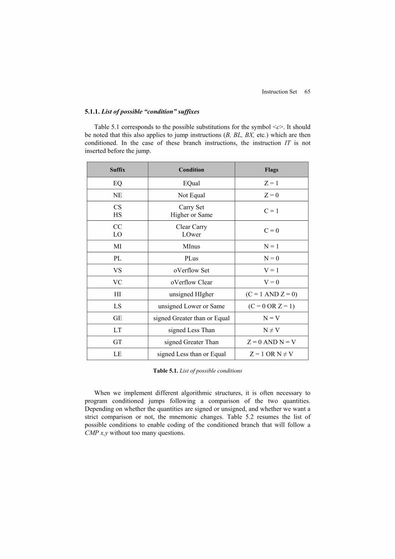
Instruction Set 65
5.1.1. List of possible “condition” suffixes
Table 5.1 corresponds to the possible substitutions for the symbol <c>. It shouldbe noted that this also applies to jump instructions (B, BL, BX, etc.) which are thenconditioned. In the case of these branch instructions, the instruction IT is notinserted before the jump.
Suffix Condition Flags
EQ EQual Z = 1
NE Not Equal Z = 0
CSHS
Carry SetHigher or Same C = 1
CCLO
Clear CarryLOwer C = 0
MI MInus N = 1
PL PLus N = 0
VS oVerflow Set V = 1
VC oVerflow Clear V = 0
HI unsigned HIgher (C = 1 AND Z = 0)
LS unsigned Lower or Same (C = 0 OR Z = 1)
GE signed Greater than or Equal N = V
LT signed Less Than N ≠ V
GT signed Greater Than Z = 0 AND N = V
LE signed Less than or Equal Z = 1 OR N ≠ V
Table 5.1. List of possible conditions
When we implement different algorithmic structures, it is often necessary toprogram conditioned jumps following a comparison of the two quantities.Depending on whether the quantities are signed or unsigned, and whether we want astrict comparison or not, the mnemonic changes. Table 5.2 resumes the list ofpossible conditions to enable coding of the conditioned branch that will follow aCMP x,y without too many questions.
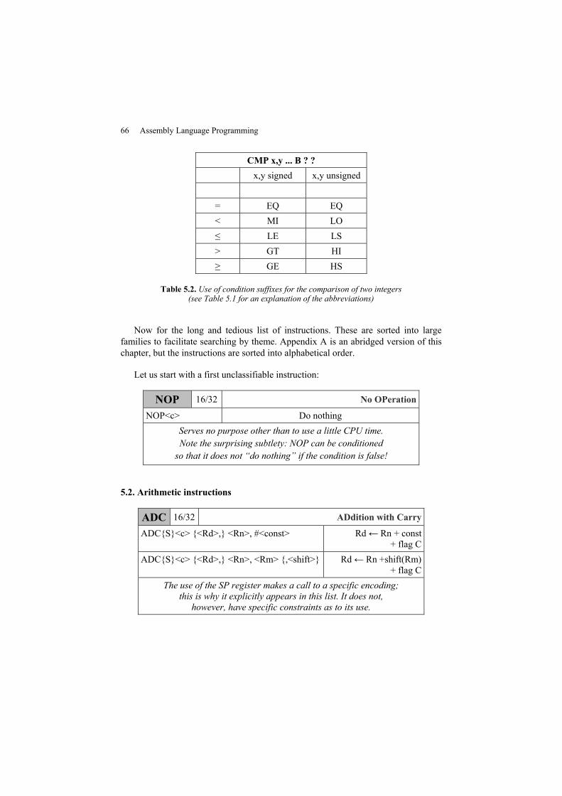
66 Assembly Language Programming
CMP x,y ... B ? ?x,y signed x,y unsigned
= EQ EQ< MI LO≤ LE LS> GT HI≥ GE HS
Table 5.2. Use of condition suffixes for the comparison of two integers(see Table 5.1 for an explanation of the abbreviations)
Now for the long and tedious list of instructions. These are sorted into largefamilies to facilitate searching by theme. Appendix A is an abridged version of thischapter, but the instructions are sorted into alphabetical order.
Let us start with a first unclassifiable instruction:
NOP 16/32 No OPeration
NOP<c> Do nothingServes no purpose other than to use a little CPU time.Note the surprising subtlety: NOP can be conditionedso that it does not “do nothing” if the condition is false!
5.2. Arithmetic instructions
ADC 16/32 ADdition with Carry
ADC{S}<c> {<Rd>,} <Rn>, #<const> Rd← Rn + const+ flag C
ADC{S}<c> {<Rd>,} <Rn>, <Rm> {,<shift>} Rd← Rn +shift(Rm)+ flag C
The use of the SP register makes a call to a specific encoding;this is why it explicitly appears in this list. It does not,however, have specific constraints as to its use.
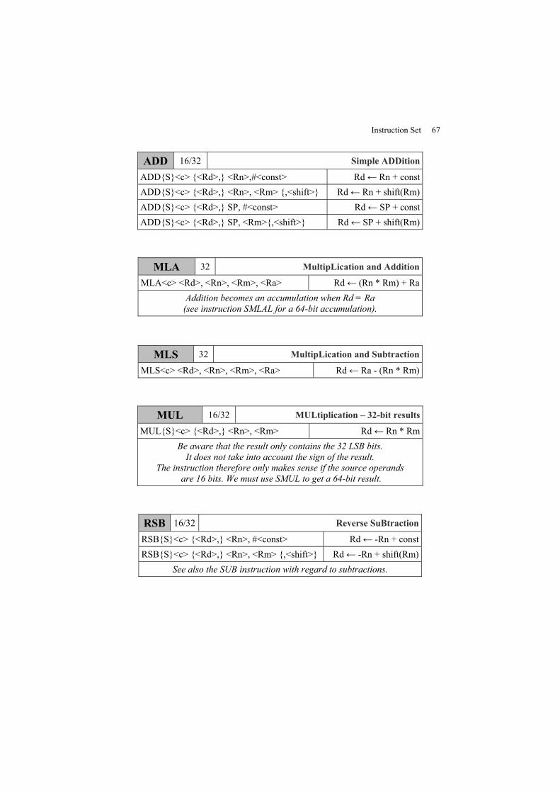
Instruction Set 67
ADD 16/32 Simple ADDition
ADD{S}<c> {<Rd>,} <Rn>,#<const> Rd← Rn + constADD{S}<c> {<Rd>,} <Rn>, <Rm> {,<shift>} Rd← Rn + shift(Rm)ADD{S}<c> {<Rd>,} SP, #<const> Rd← SP + constADD{S}<c> {<Rd>,} SP, <Rm>{,<shift>} Rd← SP + shift(Rm)
MLA 32 MultipLication and Addition
MLA<c> <Rd>, <Rn>, <Rm>, <Ra> Rd← (Rn * Rm) + RaAddition becomes an accumulation when Rd = Ra(see instruction SMLAL for a 64-bit accumulation).
MLS 32 MultipLication and Subtraction
MLS<c> <Rd>, <Rn>, <Rm>, <Ra> Rd← Ra - (Rn * Rm)
MUL 16/32 MULtiplication – 32-bit results
MUL{S}<c> {<Rd>,} <Rn>, <Rm> Rd← Rn * RmBe aware that the result only contains the 32 LSB bits.It does not take into account the sign of the result.
The instruction therefore only makes sense if the source operandsare 16 bits. We must use SMUL to get a 64-bit result.
RSB 16/32 Reverse SuBtraction
RSB{S}<c> {<Rd>,} <Rn>, #<const> Rd← -Rn + constRSB{S}<c> {<Rd>,} <Rn>, <Rm> {,<shift>} Rd← -Rn + shift(Rm)
See also the SUB instruction with regard to subtractions.
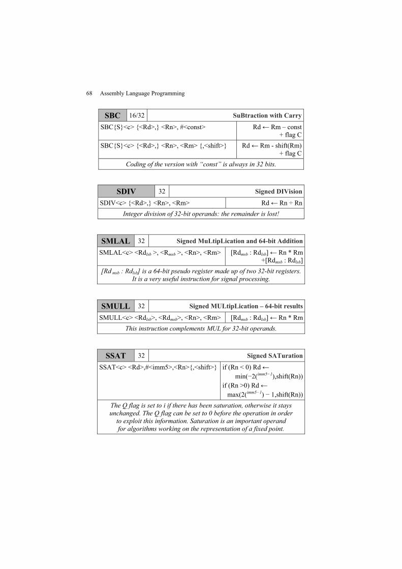
68 Assembly Language Programming
SBC 16/32 SuBtraction with Carry
SBC{S}<c> {<Rd>,} <Rn>, #<const> Rd← Rm – const+ flag C
SBC{S}<c> {<Rd>,} <Rn>, <Rm> {,<shift>} Rd← Rm - shift(Rm)+ flag C
Coding of the version with “const” is always in 32 bits.
SDIV 32 Signed DIVision
SDIV<c> {<Rd>,} <Rn>, <Rm> Rd← Rn ÷ RnInteger division of 32-bit operands: the remainder is lost!
SMLAL 32 Signed MuLtipLication and 64-bit Addition
SMLAL<c> <Rdlsb >, <Rmsb >, <Rn>, <Rm> [Rdmsb : Rdlsb]← Rn * Rm+[Rdmsb : Rdlsb]
[Rd msb : Rdlsb] is a 64-bit pseudo register made up of two 32-bit registers.It is a very useful instruction for signal processing.
SMULL 32 Signed MULtipLication – 64-bit results
SMULL<c> <Rdlsb>, <Rdmsb>, <Rn>, <Rm> [Rdmsb : Rdlsb]← Rn * RmThis instruction complements MUL for 32-bit operands.
SSAT 32 Signed SATuration
SSAT<c> <Rd>,#<imm5>,<Rn>{,<shift>} if (Rn < 0) Rd←min(−2(imm5−1),shift(Rn))
if (Rn >0) Rd←max(2(imm5−1) − 1,shift(Rn))
The Q flag is set to i if there has been saturation, otherwise it staysunchanged. The Q flag can be set to 0 before the operation in orderto exploit this information. Saturation is an important operandfor algorithms working on the representation of a fixed point.
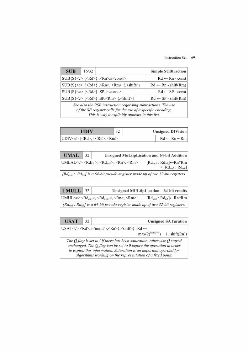
Instruction Set 69
SUB 16/32 Simple SUBtraction
SUB{S}<c> {<Rd>} ,<Rn>,#<const> Rd← Rn - constSUB{S}<c> {<Rd>} ,<Rn>, <Rm> {,<shift>} Rd← Rn - shift(Rm)SUB{S}<c> {<Rd>} ,SP,#<const> Rd← SP - constSUB{S}<c> {<Rd>} ,SP,<Rm> {,<shift>} Rd← SP - shift(Rm)
See also the RSB instruction regarding subtractions. The useof the SP register calls for the use of a specific encoding.
This is why it explicitly appears in this list.
UDIV 32 Unsigned DIVision
UDIV<c> {<Rd>,} <Rn>, <Rm> Rd← Rn ÷ Rm
UMAL 32 Unsigned MuLtipLication and 64-bit Addition
UMLAL<c> <Rdlsb >, <Rdmsb>, <Rn>, <Rm> [Rdmsb : Rdlsb]←Rn*Rm+ [Rdmsb : Rdlsb]
[Rdmsb : Rdlsb] is a 64-bit pseudo-register made up of two 32-bit registers.
UMULL 32 Unsigned MULtipLication – 64-bit results
UMUL<c> <Rdlsb >, <Rdmsb >, <Rn>, <Rm> [Rdmsb : Rdlsb]←Rn*Rm[Rdmsb : Rdlsb] is a 64-bit pseudo-register made up of two 32-bit registers.
USAT 32 Unsigned SATuration
USAT<c> <Rd>,#<imm5>,<Rn>{,<shift>} Rd←max(2(imm5−1) − 1 , shift(Rn))
The Q flag is set to i if there has been saturation, otherwise Q stayedunchanged. The Q flag can be set to 0 before the operation in orderto exploit this information. Saturation is an important operand for
algorithms working on the representation of a fixed point.
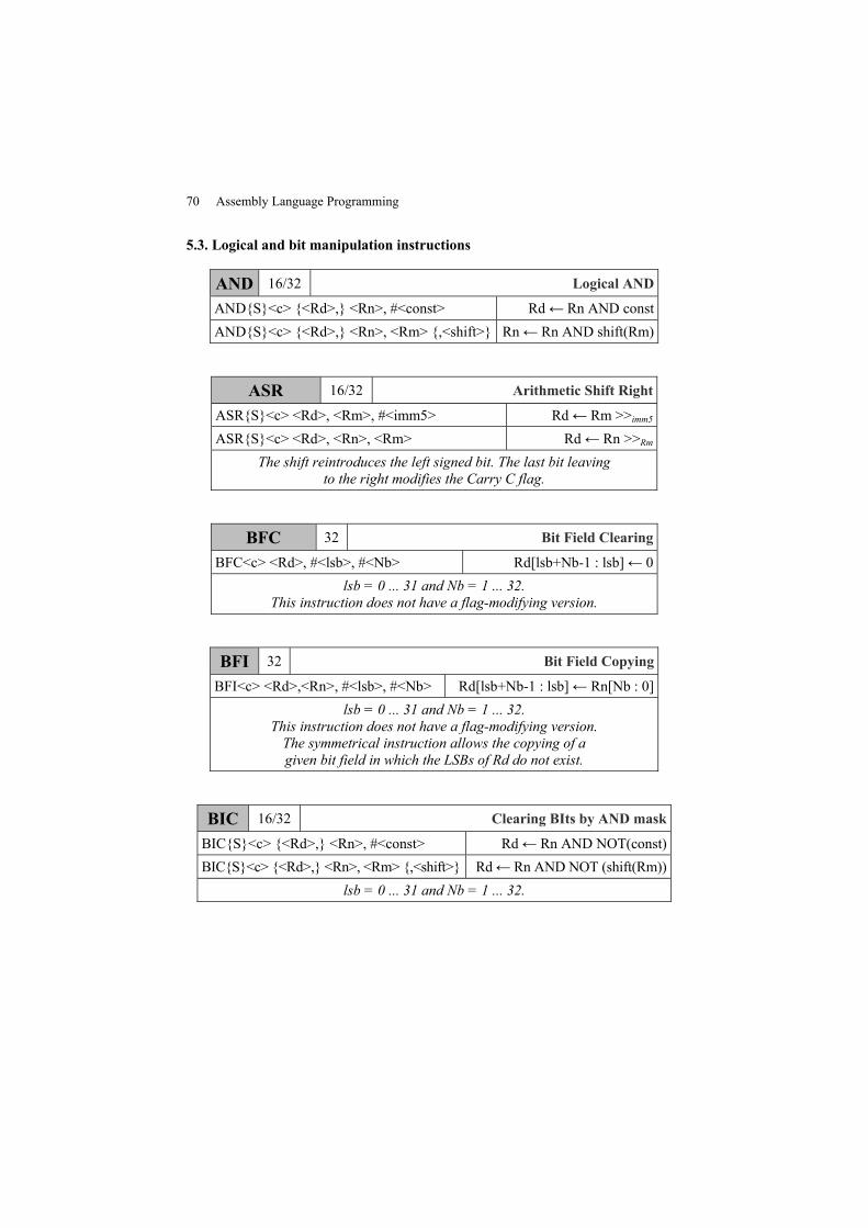
70 Assembly Language Programming
5.3. Logical and bit manipulation instructions
AND 16/32 Logical AND
AND{S}<c> {<Rd>,} <Rn>, #<const> Rd← Rn AND constAND{S}<c> {<Rd>,} <Rn>, <Rm> {,<shift>} Rn← Rn AND shift(Rm)
ASR 16/32 Arithmetic Shift Right
ASR{S}<c> <Rd>, <Rm>, #<imm5> Rd← Rm >>imm5ASR{S}<c> <Rd>, <Rn>, <Rm> Rd← Rn >>Rm
The shift reintroduces the left signed bit. The last bit leavingto the right modifies the Carry C flag.
BFC 32 Bit Field Clearing
BFC<c> <Rd>, #<lsb>, #<Nb> Rd[lsb+Nb-1 : lsb]← 0lsb = 0 ... 31 and Nb = 1 ... 32.
This instruction does not have a flag-modifying version.
BFI 32 Bit Field Copying
BFI<c> <Rd>,<Rn>, #<lsb>, #<Nb> Rd[lsb+Nb-1 : lsb]← Rn[Nb : 0]lsb = 0 ... 31 and Nb = 1 ... 32.
This instruction does not have a flag-modifying version.The symmetrical instruction allows the copying of agiven bit field in which the LSBs of Rd do not exist.
BIC 16/32 Clearing BIts by AND mask
BIC{S}<c> {<Rd>,} <Rn>, #<const> Rd← Rn AND NOT(const)BIC{S}<c> {<Rd>,} <Rn>, <Rm> {,<shift>} Rd← Rn AND NOT (shift(Rm))
lsb = 0 ... 31 and Nb = 1 ... 32.
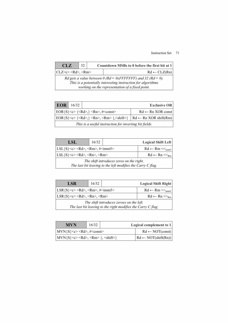
Instruction Set 71
CLZ 32 Countdown MSBs to 0 before the first bit at 1
CLZ<c> <Rd>, <Rm> Rd← CLZ(Rn)Rd gets a value between 0 (Rd = 0xFFFFFFF) and 32 (Rd = 0).
This is a potentially interesting instruction for algorithmsworking on the representation of a fixed point.
EOR 16/32 Exclusive OR
EOR{S}<c> {<Rd>,} <Rn>, #<const> Rd← Rn XOR constEOR{S}<c> {<Rd>,} <Rn>, <Rm> {,<shift>} Rd← Rn XOR shift(Rm)
This is a useful instruction for inverting bit fields.
LSL 16/32 Logical Shift Left
LSL{S}<c> <Rd>, <Rm>, #<imm5> Rd← Rm <<imm5LSL{S}<c> <Rd>, <Rn>, <Rm> Rd← Rn <<Rm
The shift introduces zeros on the right.The last bit leaving to the left modifies the Carry C flag.
LSR 16/32 Logical Shift Right
LSR{S}<c> <Rd>, <Rm>, #<imm5> Rd← Rm >>imm5LSR{S}<c> <Rd>, <Rn>, <Rm> Rd← Rn >>Rm
The shift introduces zeroes on the left.The last bit leaving to the right modifies the Carry C flag.
MVN 16/32 Logical complement to 1
MVN{S}<c> <Rd>, #<const> Rd← NOT(const)MVN{S}<c> <Rd>, <Rm> {, <shift>} Rd← NOT(shift(Rn))
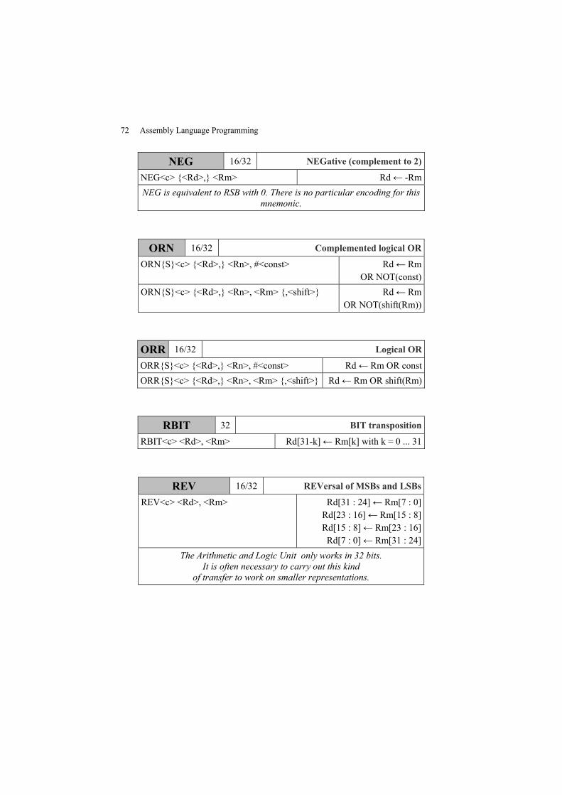
72 Assembly Language Programming
NEG 16/32 NEGative (complement to 2)
NEG<c> {<Rd>,} <Rm> Rd← -RmNEG is equivalent to RSB with 0. There is no particular encoding for this
mnemonic.
ORN 16/32 Complemented logical OR
ORN{S}<c> {<Rd>,} <Rn>, #<const> Rd← RmOR NOT(const)
ORN{S}<c> {<Rd>,} <Rn>, <Rm> {,<shift>} Rd← RmOR NOT(shift(Rm))
ORR 16/32 Logical OR
ORR{S}<c> {<Rd>,} <Rn>, #<const> Rd← Rm OR constORR{S}<c> {<Rd>,} <Rn>, <Rm> {,<shift>} Rd← Rm OR shift(Rm)
RBIT 32 BIT transposition
RBIT<c> <Rd>, <Rm> Rd[31-k]← Rm[k] with k = 0 ... 31
REV 16/32 REVersal of MSBs and LSBs
REV<c> <Rd>, <Rm> Rd[31 : 24]← Rm[7 : 0]Rd[23 : 16]← Rm[15 : 8]Rd[15 : 8]← Rm[23 : 16]Rd[7 : 0]← Rm[31 : 24]
The Arithmetic and Logic Unit only works in 32 bits.It is often necessary to carry out this kind
of transfer to work on smaller representations.
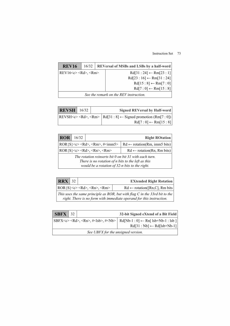
Instruction Set 73
REV16 16/32 REVersal of MSBs and LSBs by a half-word
REV16<c> <Rd>, <Rm> Rd[31 : 24]← Rm[23 : 1]Rd[23 : 16]← Rm[31 : 24]
Rd[15 : 8]← Rm[7 : 0]Rd[7 : 0]← Rm[15 : 8]
See the remark on the REV instruction.
REVSH 16/32 Signed REVersal by Half-word
REVSH<c> <Rd>, <Rm> Rd[31 : 8]← Signed promotion (Rm[7 : 0])Rd[7 : 0]← Rm[15 : 8]
ROR 16/32 Right ROtation
ROR{S}<c> <Rd>, <Rm>, #<imm5> Rd← rotation(Rm, imm5 bits)ROR{S}<c> <Rd>, <Rn>, <Rm> Rd← rotation(Rn, Rm bits)
The rotation reinserts bit 0 on bit 31 with each turn.There is no rotation of n bits to the left as thiswould be a rotation of 32-n bits to the right.
RRX 32 EXtended Right Rotation
ROR{S}<c> <Rd>, <Rn>, <Rm> Rd← rotation([Rn,C], Rm bitsThis uses the same principle as ROR, but with flag C in the 33rd bit to theright. There is no form with immediate operand for this instruction.
SBFX 32 32-bit Signed eXtend of a Bit Field
SBFX<c> <Rd>, <Rn>, #<lsb>, #<Nb> Rd[Nb-1 : 0]← Rn[ lsb+Nb-1 : lsb ]Rd[31 : Nb]← Rd[lsb+Nb-1]
See UBFX for the unsigned version.
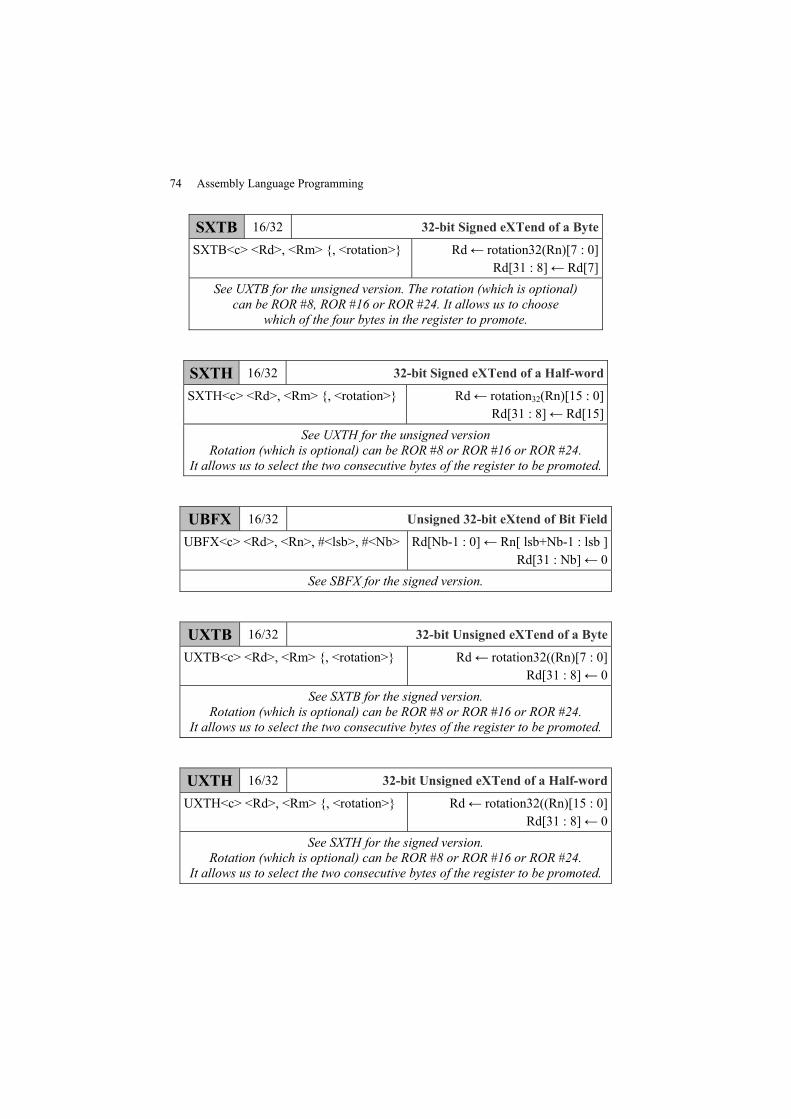
74 Assembly Language Programming
SXTB 16/32 32-bit Signed eXTend of a Byte
SXTB<c> <Rd>, <Rm> {, <rotation>} Rd← rotation32(Rn)[7 : 0]Rd[31 : 8]← Rd[7]
See UXTB for the unsigned version. The rotation (which is optional)can be ROR #8, ROR #16 or ROR #24. It allows us to choose
which of the four bytes in the register to promote.
SXTH 16/32 32-bit Signed eXTend of a Half-word
SXTH<c> <Rd>, <Rm> {, <rotation>} Rd← rotation32(Rn)[15 : 0]Rd[31 : 8]← Rd[15]
See UXTH for the unsigned versionRotation (which is optional) can be ROR #8 or ROR #16 or ROR #24.
It allows us to select the two consecutive bytes of the register to be promoted.
UBFX 16/32 Unsigned 32-bit eXtend of Bit Field
UBFX<c> <Rd>, <Rn>, #<lsb>, #<Nb> Rd[Nb-1 : 0]← Rn[ lsb+Nb-1 : lsb ]Rd[31 : Nb]← 0
See SBFX for the signed version.
UXTB 16/32 32-bit Unsigned eXTend of a Byte
UXTB<c> <Rd>, <Rm> {, <rotation>} Rd← rotation32((Rn)[7 : 0]Rd[31 : 8]← 0
See SXTB for the signed version.Rotation (which is optional) can be ROR #8 or ROR #16 or ROR #24.
It allows us to select the two consecutive bytes of the register to be promoted.
UXTH 16/32 32-bit Unsigned eXTend of a Half-word
UXTH<c> <Rd>, <Rm> {, <rotation>} Rd← rotation32((Rn)[15 : 0]Rd[31 : 8]← 0
See SXTH for the signed version.Rotation (which is optional) can be ROR #8 or ROR #16 or ROR #24.
It allows us to select the two consecutive bytes of the register to be promoted.
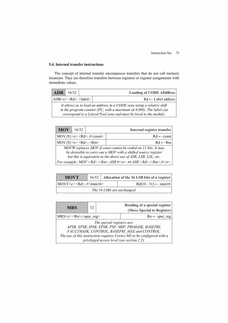
Instruction Set 75
5.4. Internal transfer instructions
The concept of internal transfer encompasses transfers that do not call memorylocations. They are therefore transfers between registers or register assignments withimmediate values.
ADR 16/32 Loading of CODE ADdRess
ADR<c> <Rd>, <label> Rd← Label addressIt allows us to load an address in a CODE zone using a relative shiftin the program counter (PC, with a maximum of 4,096). The label cancorrespond to a Literal Pool zone and must be local to the module.
MOV 16/32 Internal register transfer
MOV{S}<c> <Rd>, #<const> Rd← constMOV{S}<c> <Rd>, <Rm> Rd← Rm
MOVW replaces MOV if const cannot be coded on 11 bits. It maybe desirable to carry out a MOV with a shifted source registerbut this is equivalent to the direct use of ASR, LSR, LSL, etc.
For example: MOV <Rd>,<Rm>,ASR #<n>⇔ ASR <Rd>,<Rm>,#<n>.
MOVT 16/32 Allocation of the 16 LSB bits of a register
MOVT<c> <Rd>, #<imm16> Rd[16 : 31]← imm16The 16 LSBs are unchanged.
MRS 32Reading of a special register(Move Special to Register)
MRS<c> <Rn>,<spec_reg> Rn← spec_regThe special registers are:
APSR, XPSR, IPSR, EPSR, PSP, MSP, PRIMASK, BASEPRI,FAULTMASK, CONTROL, BASEPRI_MAX and CONTROL.
The use of this instruction requires Cortex-M3 to be configured with aprivileged access level (see section 2.2).
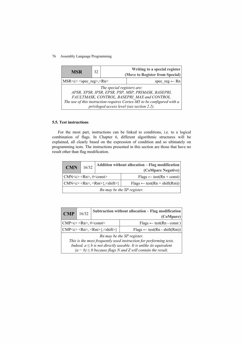
76 Assembly Language Programming
MSR 32Writing to a special register
(Move to Register from Special)MSR<c> <spec_reg>,<Rn> spec_reg← Rn
The special registers are:APSR, XPSR, IPSR, EPSR, PSP, MSP, PRIMASK, BASEPRI,FAULTMASK, CONTROL, BASEPRI_MAX and CONTROL.
The use of this instruction requires Cortex-M3 to be configured with aprivileged access level (see section 2.2).
5.5. Test instructions
For the most part, instructions can be linked to conditions, i.e. to a logicalcombination of flags. In Chapter 6, different algorithmic structures will beexplained, all clearly based on the expression of condition and so ultimately onprogramming tests. The instructions presented in this section are those that have noresult other than flag modification.
CMN 16/32Addition without allocation – Flag modification
(CoMpare Negative)CMN<c> <Rn>, #<const> Flags← test(Rn + const)CMN<c> <Rn>, <Rm>{,<shift>} Flags← test(Rn + shift(Rm))
Rn may be the SP register.
CMP 16/32Subtraction without allocation – Flag modification
(CoMpare)CMP<c> <Rn>, #<const> Flags← test(Rn - const )CMP<c> <Rn>, <Rm>{,<shift>} Flags← test(Rn - shift(Rm))
Rn may be the SP register.This is the most frequently used instruction for performing tests.Indeed, a ≤ b is not directly useable. It is unlike its equivalent(a − b) ≤ 0 because flags N and Z will contain the result.
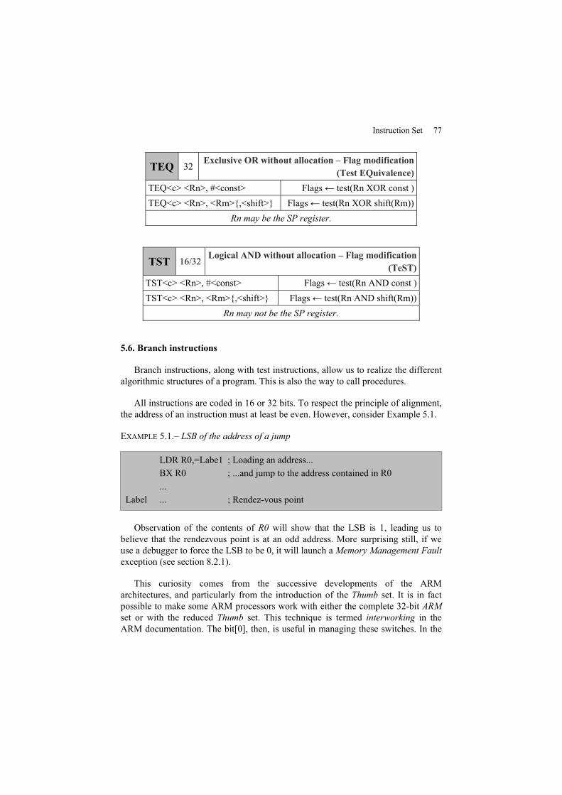
Instruction Set 77
TEQ 32Exclusive OR without allocation – Flag modification
(Test EQuivalence)TEQ<c> <Rn>, #<const> Flags← test(Rn XOR const )TEQ<c> <Rn>, <Rm>{,<shift>} Flags← test(Rn XOR shift(Rm))
Rn may be the SP register.
TST 16/32Logical AND without allocation – Flag modification
(TeST)TST<c> <Rn>, #<const> Flags← test(Rn AND const )TST<c> <Rn>, <Rm>{,<shift>} Flags← test(Rn AND shift(Rm))
Rn may not be the SP register.
5.6. Branch instructions
Branch instructions, along with test instructions, allow us to realize the differentalgorithmic structures of a program. This is also the way to call procedures.
All instructions are coded in 16 or 32 bits. To respect the principle of alignment,the address of an instruction must at least be even. However, consider Example 5.1.
EXAMPLE 5.1.– LSB of the address of a jump
LDR R0,=Labe1 ; Loading an address...BX R0 ; ...and jump to the address contained in R0...
Label ... ; Rendez-vous point
Observation of the contents of R0 will show that the LSB is 1, leading us tobelieve that the rendezvous point is at an odd address. More surprising still, if weuse a debugger to force the LSB to be 0, it will launch a Memory Management Faultexception (see section 8.2.1).
This curiosity comes from the successive developments of the ARMarchitectures, and particularly from the introduction of the Thumb set. It is in factpossible to make some ARM processors work with either the complete 32-bit ARMset or with the reduced Thumb set. This technique is termed interworking in theARM documentation. The bit[0], then, is useful in managing these switches. In the
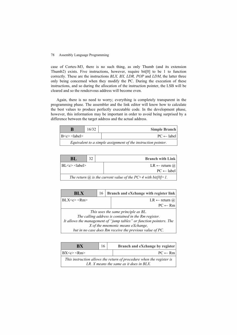
78 Assembly Language Programming
case of Cortex-M3, there is no such thing, as only Thumb (and its extensionThumb2) exists. Five instructions, however, require bit[0] to be 1 to functioncorrectly. These are the instructions BLX, BX, LDR, POP and LDM, the latter threeonly being concerned when they modify the PC. During the execution of theseinstructions, and so during the allocation of the instruction pointer, the LSB will becleared and so the rendezvous address will become even.
Again, there is no need to worry; everything is completely transparent in theprogramming phase. The assembler and the link editor will know how to calculatethe best values to produce perfectly executable code. In the development phase,however, this information may be important in order to avoid being surprised by adifference between the target address and the actual address.
B 16/32 Simple Branch
B<c> <label> PC← labelEquivalent to a simple assignment of the instruction pointer.
BL 32 Branch with Link
BL<c> <label> LR← return @PC← label
The return @ is the current value of the PC+4 with bit[0]=1.
BLX 16 Branch and eXchange with register link
BLX<c> <Rm> LR← return @PC← Rm
This uses the same principle as BL.The calling address is contained in the Rm register.
It allows the management of “jump tables” or function pointers. TheX of the mnemonic means eXchange,
but in no case does Rm receive the previous value of PC.
BX 16 Branch and eXchange by register
BX<c> <Rm> PC← RmThis instruction allows the return of procedure when the register is
LR. X means the same as it does in BLX.
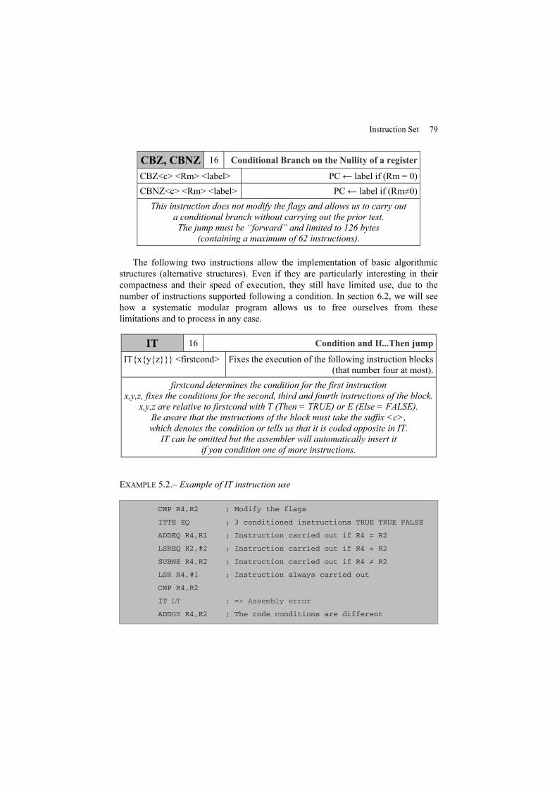
Instruction Set 79
CBZ, CBNZ 16 Conditional Branch on the Nullity of a register
CBZ<c> <Rm> <label> PC← label if (Rm = 0)CBNZ<c> <Rm> <label> PC← label if (Rm≠0)This instruction does not modify the flags and allows us to carry out
a conditional branch without carrying out the prior test.The jump must be “forward” and limited to 126 bytes
(containing a maximum of 62 instructions).
The following two instructions allow the implementation of basic algorithmicstructures (alternative structures). Even if they are particularly interesting in theircompactness and their speed of execution, they still have limited use, due to thenumber of instructions supported following a condition. In section 6.2, we will seehow a systematic modular program allows us to free ourselves from theselimitations and to process in any case.
IT 16 Condition and If...Then jump
IT{x{y{z}}} <firstcond> Fixes the execution of the following instruction blocks(that number four at most).
firstcond determines the condition for the first instructionx,y,z, fixes the conditions for the second, third and fourth instructions of the block.
x,y,z are relative to firstcond with T (Then = TRUE) or E (Else = FALSE).Be aware that the instructions of the block must take the suffix <c>,which denotes the condition or tells us that it is coded opposite in IT.IT can be omitted but the assembler will automatically insert it
if you condition one of more instructions.
EXAMPLE 5.2.– Example of IT instruction use
CMP R4,R2 ; Modify the flags
ITTE EQ ; 3 conditioned instructions TRUE TRUE FALSE
ADDEQ R4,R1 ; Instruction carried out if R4 = R2
LSREQ R2,#2 ; Instruction carried out if R4 = R2
SUBNE R4,R2 ; Instruction carried out if R4 ≠ R2
LSR R4,#1 ; Instruction always carried out
CMP R4,R2
IT LT ; => Assembly error
ADDGE R4,R2 ; The code conditions are different
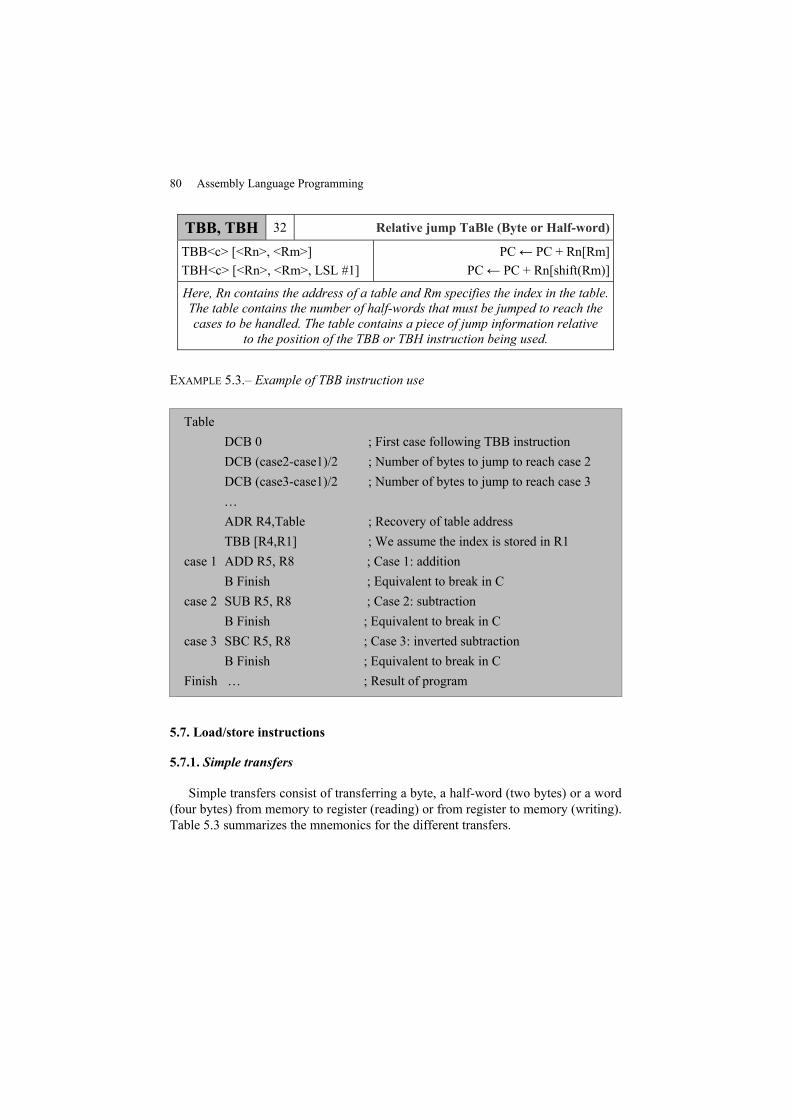
80 Assembly Language Programming
TBB, TBH 32 Relative jump TaBle (Byte or Half-word)
TBB<c> [<Rn>, <Rm>]TBH<c> [<Rn>, <Rm>, LSL #1]
PC← PC + Rn[Rm]PC← PC + Rn[shift(Rm)]
Here, Rn contains the address of a table and Rm specifies the index in the table.The table contains the number of half-words that must be jumped to reach thecases to be handled. The table contains a piece of jump information relative
to the position of the TBB or TBH instruction being used.
EXAMPLE 5.3.– Example of TBB instruction use
TableDCB 0 ; First case following TBB instructionDCB (case2-case1)/2 ; Number of bytes to jump to reach case 2DCB (case3-case1)/2 ; Number of bytes to jump to reach case 3…ADR R4,Table ; Recovery of table addressTBB [R4,R1] ; We assume the index is stored in R1
case 1 ADD R5, R8 ; Case 1: additionB Finish ; Equivalent to break in C
case 2 SUB R5, R8 ; Case 2: subtractionB Finish ; Equivalent to break in C
case 3 SBC R5, R8 ; Case 3: inverted subtractionB Finish ; Equivalent to break in C
Finish … ; Result of program
5.7. Load/store instructions
5.7.1. Simple transfers
Simple transfers consist of transferring a byte, a half-word (two bytes) or a word(four bytes) from memory to register (reading) or from register to memory (writing).Table 5.3 summarizes the mnemonics for the different transfers.
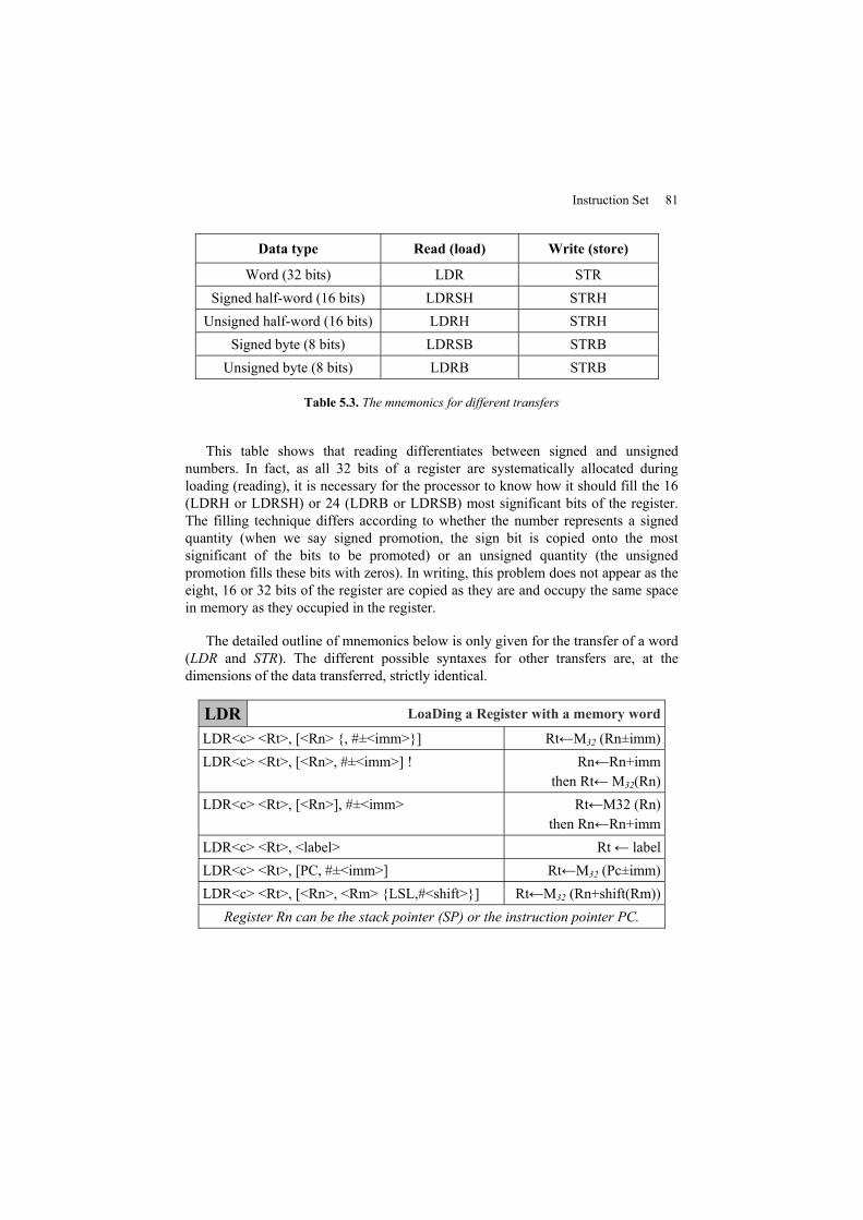
Instruction Set 81
Data type Read (load) Write (store)
Word (32 bits) LDR STRSigned half-word (16 bits) LDRSH STRHUnsigned half-word (16 bits) LDRH STRH
Signed byte (8 bits) LDRSB STRBUnsigned byte (8 bits) LDRB STRB
Table 5.3. The mnemonics for different transfers
This table shows that reading differentiates between signed and unsignednumbers. In fact, as all 32 bits of a register are systematically allocated duringloading (reading), it is necessary for the processor to know how it should fill the 16(LDRH or LDRSH) or 24 (LDRB or LDRSB) most significant bits of the register.The filling technique differs according to whether the number represents a signedquantity (when we say signed promotion, the sign bit is copied onto the mostsignificant of the bits to be promoted) or an unsigned quantity (the unsignedpromotion fills these bits with zeros). In writing, this problem does not appear as theeight, 16 or 32 bits of the register are copied as they are and occupy the same spacein memory as they occupied in the register.
The detailed outline of mnemonics below is only given for the transfer of a word(LDR and STR). The different possible syntaxes for other transfers are, at thedimensions of the data transferred, strictly identical.
LDR LoaDing a Register with a memory word
LDR<c> <Rt>, [<Rn> {, #±<imm>}] Rt←M32 (Rn±imm)LDR<c> <Rt>, [<Rn>, #±<imm>] ! Rn←Rn+imm
then Rt←M32(Rn)LDR<c> <Rt>, [<Rn>], #±<imm> Rt←M32 (Rn)
then Rn←Rn+immLDR<c> <Rt>, <label> Rt← labelLDR<c> <Rt>, [PC, #±<imm>] Rt←M32 (Pc±imm)LDR<c> <Rt>, [<Rn>, <Rm> {LSL,#<shift>}] Rt←M32 (Rn+shift(Rm))
Register Rn can be the stack pointer (SP) or the instruction pointer PC.
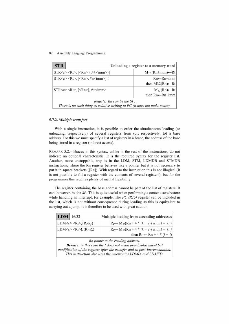
82 Assembly Language Programming
STR Unloading a register to a memory word
STR<c> <Rt>, [<Rn> {,#±<imm>}] M32 (Rn±imm)←RtSTR<c> <Rt>, [<Rn>, #±<imm>] ! Rn←Rn+imm
then M32(Rn)←RtSTR<c> <Rt>, [<Rn>], #±<imm> M32 (Rn)←Rt
then Rn←Rn+immRegister Rn can be the SP.
There is no such thing as relative writing to PC (it does not make sense).
5.7.2.Multiple transfers
With a single instruction, it is possible to order the simultaneous loading (orunloading, respectively) of several registers from (or, respectively, to) a baseaddress. For this we must specify a list of registers in a brace, the address of the basebeing stored in a register (indirect access).
REMARK 5.2.– Braces in this syntax, unlike in the rest of the instructions, do notindicate an optional characteristic. It is the required syntax for the register list.Another, more unstoppable, trap is in the LDM, STM, LDMDB and STMDBinstructions, where the Rn register behaves like a pointer but it is not necessary toput it in square brackets ([Rn]). With regard to the instruction this is not illogical (itis not possible to fill a register with the contents of several registers), but for theprogrammer this requires plenty of mental flexibility.
The register containing the base address cannot be part of the list of registers. Itcan, however, be the SP. This is quite useful when performing a context save/restorewhile handling an interrupt, for example. The PC (R15) register can be included inthe list, which is not without consequence during loading as this is equivalent tocarrying out a jump. It is therefore to be used with great caution.
LDM 16/32 Multiple loading from ascending addresses
LDM<c> <Rk>,{Ri-Rj} Rk←M32(Rn + 4 * (k − i)) with k = i...jLDM<c> <Rk>!,{Ri-Rj} Rk←M32(Rn + 4 * (k − i)) with k = i...j
then Rn← Rn + 4 * (j − i)Rn points to the reading address.
Beware: in this case the ! does not mean pre-displacement butmodification of the register after the transfer and so post-incrementation.
This instruction also uses the mnemonics LDMIA and LDMFD.
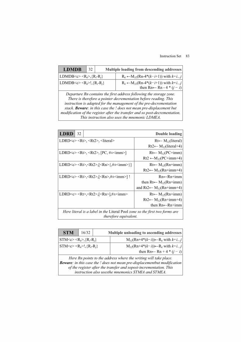
Instruction Set 83
LDMDB 32 Multiple loading from descending addresses
LDMDB<c> <Rk>,{Ri-Rj} Rk ←M32(Rn-4*(k−i+1)) with k=i...jLDMDB<c> <Rk>!,{Ri-Rj} Rk ←M32(Rn-4*(k−i+1)) with k=i...j
then Rn← Rn - 4 * (j − i)Departure Rn contains the first address following the storage zone.There is therefore a pointer decrementation before reading. This
instruction is adapted for the management of the pre-decrementationstack. Beware: in this case the ! does not mean pre-displacement but
modification of the register after the transfer and so post-decrementation.This instruction also uses the mnemonic LDMEA.
LDRD 32 Double loading
LDRD<c> <Rt>, <Rt2>, <literal> Rt←M32(literal)Rt2←M32(literal+4)
LDRD<c> <Rt>, <Rt2>, [PC, #±<imm>] Rt←M32(PC+imm)Rt2←M32(PC+imm+4)
LDRD<c> <Rt>,<Rt2>,[<Rn>{,#±<imm>}] Rt←M32(Rn+imm)Rt2←M32(Rn+imm+4)
LDRD<c> <Rt>,<Rt2>,[<Rn>,#±<imm>] ! Rn←Rn+immthen Rt←M32(Rn+imm)
and Rt2←M32(Rn+imm+4)LDRD<c> <Rt>,<Rt2>,[<Rn>],#±<imm> Rt←M32(Rn+imm)
Rt2←M32(Rn+imm+4)then Rn←Rn+imm
Here literal is a label in the Literal Pool zone so the first two forms aretherefore equivalent.
STM 16/32 Multiple unloading to ascending addresses
STM<c> <Rk>,{Ri-Rj} M32(Rn+4*(k−i))←Rk with k=i...jSTM<c> <Rk>!,{Ri-Rj} M32(Rn+4*(k−i))←Rk with k=i...j
then Rn← Rn + 4 * (j − i)Here Rn points to the address where the writing will take place.
Beware: in this case the ! does not mean pre-displacementbut modificationof the register after the transfer and sopost-incrementation. This
instruction also usesthe mnemonics STMIA and STMEA.
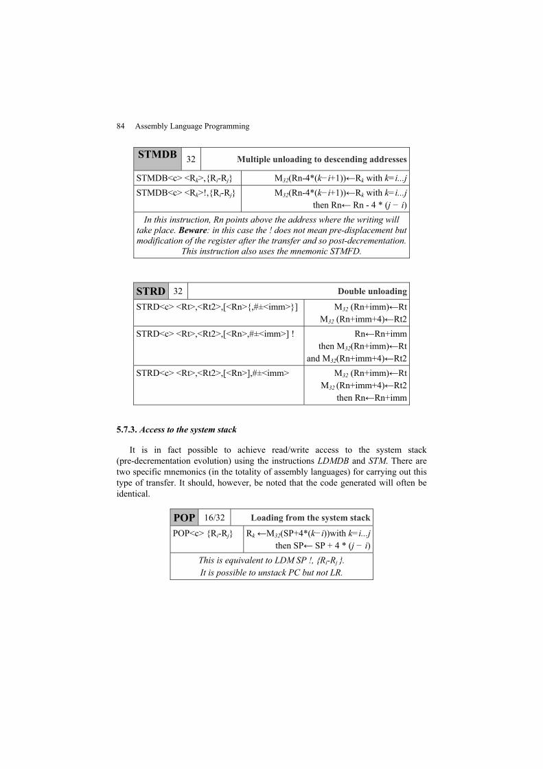
84 Assembly Language Programming
STMDB 32 Multiple unloading to descending addresses
STMDB<c> <Rk>,{Ri-Rj} M32(Rn-4*(k−i+1))←Rk with k=i...jSTMDB<c> <Rk>!,{Ri-Rj} M32(Rn-4*(k−i+1))←Rk with k=i...j
then Rn← Rn - 4 * (j − i)In this instruction, Rn points above the address where the writing will
take place. Beware: in this case the ! does not mean pre-displacement butmodification of the register after the transfer and so post-decrementation.
This instruction also uses the mnemonic STMFD.
STRD 32 Double unloading
STRD<c> <Rt>,<Rt2>,[<Rn>{,#±<imm>}] M32 (Rn+imm)←RtM32 (Rn+imm+4)←Rt2
STRD<c> <Rt>,<Rt2>,[<Rn>,#±<imm>] ! Rn←Rn+immthen M32(Rn+imm)←Rt
and M32(Rn+imm+4)←Rt2STRD<c> <Rt>,<Rt2>,[<Rn>],#±<imm> M32 (Rn+imm)←Rt
M32 (Rn+imm+4)←Rt2then Rn←Rn+imm
5.7.3. Access to the system stack
It is in fact possible to achieve read/write access to the system stack(pre-decrementation evolution) using the instructions LDMDB and STM. There aretwo specific mnemonics (in the totality of assembly languages) for carrying out thistype of transfer. It should, however, be noted that the code generated will often beidentical.
POP 16/32 Loading from the system stack
POP<c> {Ri-Rj} Rk ←M32(SP+4*(k−i))with k=i...jthen SP← SP + 4 * (j − i)
This is equivalent to LDM SP !, {Ri-Rj }.It is possible to unstack PC but not LR.
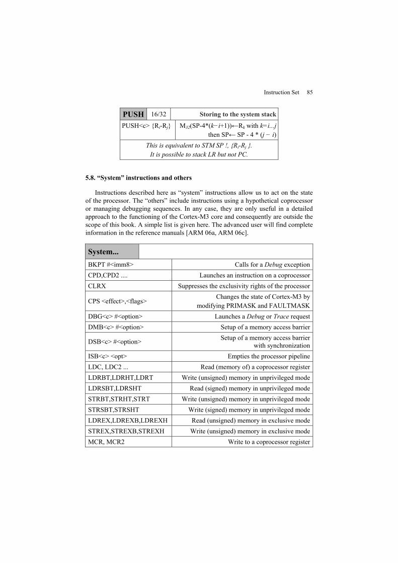
Instruction Set 85
PUSH 16/32 Storing to the system stack
PUSH<c> {Ri-Rj} M32(SP-4*(k−i+1))←Rk with k=i...jthen SP← SP - 4 * (j − i)
This is equivalent to STM SP !, {Ri-Rj }.It is possible to stack LR but not PC.
5.8. “System” instructions and others
Instructions described here as “system” instructions allow us to act on the stateof the processor. The “others” include instructions using a hypothetical coprocessoror managing debugging sequences. In any case, they are only useful in a detailedapproach to the functioning of the Cortex-M3 core and consequently are outside thescope of this book. A simple list is given here. The advanced user will find completeinformation in the reference manuals [ARM 06a, ARM 06c].
System...BKPT #<imm8> Calls for a Debug exceptionCPD,CPD2 .... Launches an instruction on a coprocessorCLRX Suppresses the exclusivity rights of the processor
CPS <effect>,<flags>Changes the state of Cortex-M3 by
modifying PRIMASK and FAULTMASKDBG<c> #<option> Launches a Debug or Trace requestDMB<c> #<option> Setup of a memory access barrier
DSB<c> #<option> Setup of a memory access barrierwith synchronization
ISB<c> <opt> Empties the processor pipelineLDC, LDC2 ... Read (memory of) a coprocessor registerLDRBT,LDRHT,LDRT Write (unsigned) memory in unprivileged modeLDRSBT,LDRSHT Read (signed) memory in unprivileged modeSTRBT,STRHT,STRT Write (unsigned) memory in unprivileged modeSTRSBT,STRSHT Write (signed) memory in unprivileged modeLDREX,LDREXB,LDREXH Read (unsigned) memory in exclusive modeSTREX,STREXB,STREXH Write (unsigned) memory in exclusive modeMCR, MCR2 Write to a coprocessor register
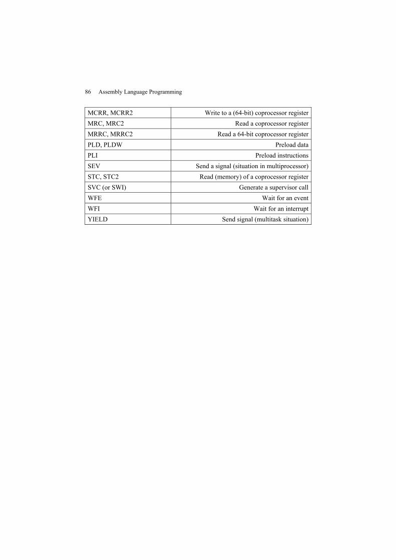
86 Assembly Language Programming
MCRR, MCRR2 Write to a (64-bit) coprocessor registerMRC, MRC2 Read a coprocessor registerMRRC, MRRC2 Read a 64-bit coprocessor registerPLD, PLDW Preload dataPLI Preload instructionsSEV Send a signal (situation in multiprocessor)STC, STC2 Read (memory) of a coprocessor registerSVC (or SWI) Generate a supervisor callWFE Wait for an eventWFI Wait for an interruptYIELD Send signal (multitask situation)
Chapter 6
Algorithmic and Data Structures
6.1. Flowchart versus algorithm
Assembly language uses labels and jumps, which can be conditional or not. Thisnaturally leads to a geographic vision of a program, where we represent the routeplan (route map) of the instructions in the form of a flowchart, with agreed symbolsto represent the conditional diversions (switches), among others. Such use offlowcharts was abandoned long ago, however, in favor of writing structuredalgorithms for various reasons. Here are some of them:
– the design and maintenance of a flowchart is laborious;
– the debugging of programs is also laborious: if there is a problem in theexecution of an instruction, it is not obvious which route in the flowchart we took toreach this point;
– it is very difficult to test just part of a program;
– it is also very difficult to extract part of a program from a flowchart in order toreuse it in a subsequent program.
We therefore prefer to encourage a tree analysis, known as modular analysis, inwhich every program is exclusively made up of a succession of cellular elements,generically called modules, each module itself being a series of sub-modules, etc. Atthe most basic level, we arrive at the idea of a structured language made up ofinstructions that, like the modules, only have one entry point and one exit point. Inthis way it is possible to obtain structured language when we program correctly.
88 Assembly Language Programming
In assembly language, we have at best transposed these concepts: the programcan be written to different files (called “modules” in the jargon used elsewhere byassemblyists), which make up what is known as external modularity. Each file ismade up of procedures, which themselves call subroutines, etc. This is known asinternal modularity. Each module or procedure represents a piece of the program: itmust be able to be tested separately, and to be reused later in another program. Atthe deepest level of this ideal tree structure, we find the instruction. In noting thateach module only has one entry point and one exit point, the instruction must alsoonly have one entrance and one exit. There is a catch with assembly language,however, since assembly language is not a structured language! Some instructions,such as conditional instructions, for example, have two exits. Despite this, weapproach programming in assembly language in a structured manner: we get aroundthe problem with so-called systematic programming. The lowest level modules arefirst described with a structured algorithm. Then, for each structured instruction inthe algorithm, we systematically transcribe it into assembly language according to amodel prepared in advance. Each structured instruction then corresponds to a blockmade up of lines of instructions in assembly language. This block has only one entrypoint (the first instruction) and one exit point. If there are labels in this block, wemust consider them specific to this block, and inaccessible to other external blocks.The only label accessible to the outside world is the entry label, which is posted onthe first instruction of the sealed block. In this chapter, we will show how eachstructured instruction can be transformed into a block of assembly languageinstructions. For each block of instructions presented, we will use the labelsEntry_Point and Exit_Point to show the entry and exit points of the block.Structured instructions in algorithmic language use the following conventions:
– cond represents a Boolean condition;
– not(cond) is the logical opposite of cond;
– treatment is a sequence of instructions to be executed;
– variable is an integer datum.
It should be noted that, for the sake of readability of an assembly languageprogram, it is strongly recommended that each block contains a maximum of about10 lines. Treatment can then be made up of several simple instructions, or elsecalling procedures. We should note that the label names have been chosen tocorrespond as closely as possible to those that appear in the algorithms, but weshould also be aware that these names or this method of choosing labels in a realprogram would be a very bad idea.
REMARK 6.1.– In this chapter we will present the different algorithmic structures,purposely omitting an instruction peculiar to the ARM assembler: IT (InTerrupt)(meaning the option to condition most arithmetic and logical instructions). This
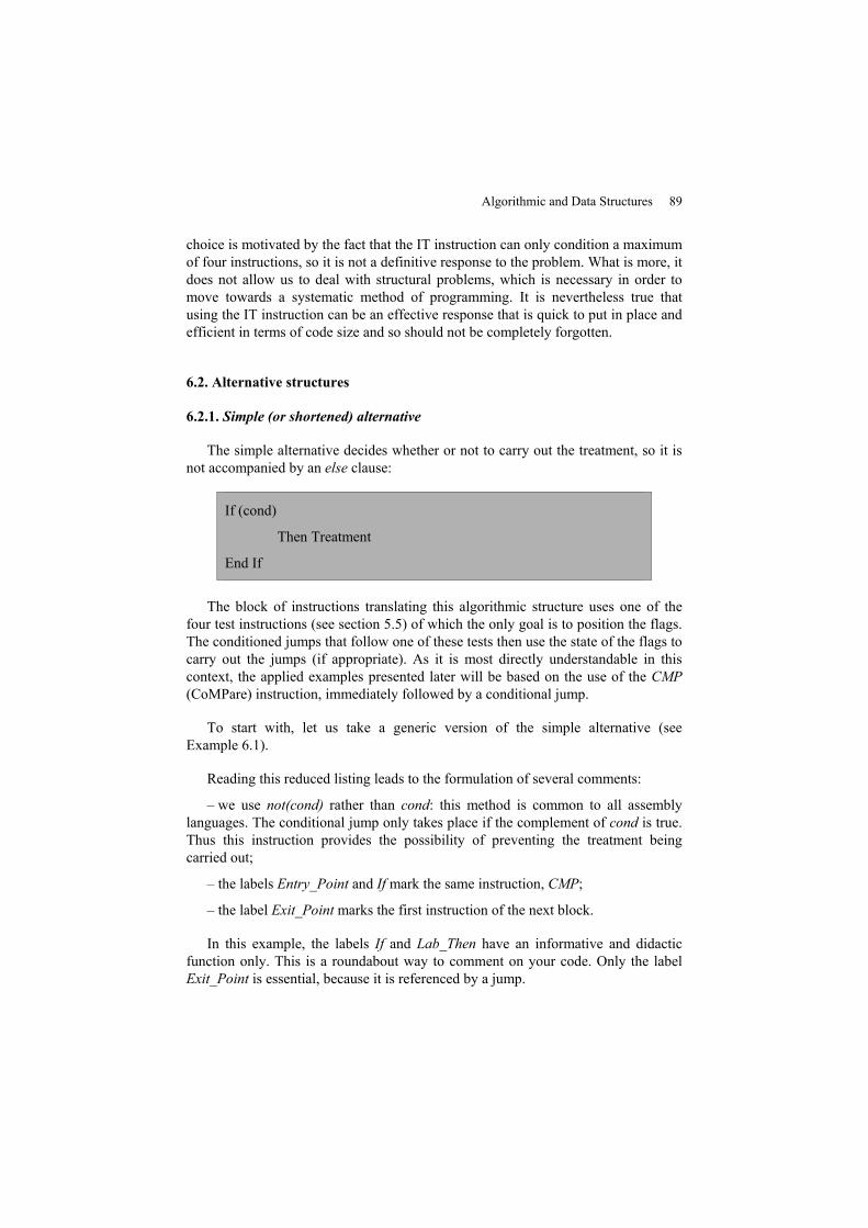
Algorithmic and Data Structures 89
choice is motivated by the fact that the IT instruction can only condition a maximumof four instructions, so it is not a definitive response to the problem. What is more, itdoes not allow us to deal with structural problems, which is necessary in order tomove towards a systematic method of programming. It is nevertheless true thatusing the IT instruction can be an effective response that is quick to put in place andefficient in terms of code size and so should not be completely forgotten.
6.2. Alternative structures
6.2.1. Simple (or shortened) alternative
The simple alternative decides whether or not to carry out the treatment, so it isnot accompanied by an else clause:
If (cond)
Then Treatment
End If
The block of instructions translating this algorithmic structure uses one of thefour test instructions (see section 5.5) of which the only goal is to position the flags.The conditioned jumps that follow one of these tests then use the state of the flags tocarry out the jumps (if appropriate). As it is most directly understandable in thiscontext, the applied examples presented later will be based on the use of the CMP(CoMPare) instruction, immediately followed by a conditional jump.
To start with, let us take a generic version of the simple alternative (seeExample 6.1).
Reading this reduced listing leads to the formulation of several comments:
– we use not(cond) rather than cond: this method is common to all assemblylanguages. The conditional jump only takes place if the complement of cond is true.Thus this instruction provides the possibility of preventing the treatment beingcarried out;
– the labels Entry_Point and If mark the same instruction, CMP;
– the label Exit_Point marks the first instruction of the next block.
In this example, the labels If and Lab_Then have an informative and didacticfunction only. This is a roundabout way to comment on your code. Only the labelExit_Point is essential, because it is referenced by a jump.
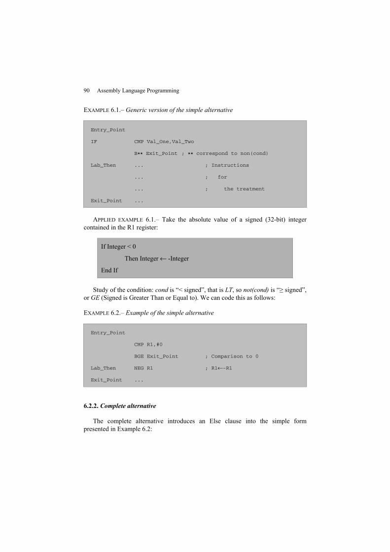
90 Assembly Language Programming
EXAMPLE 6.1.– Generic version of the simple alternative
Entry_Point
IF CMP Val_One,Val_Two
B⋆⋆ Exit_Point ; ⋆⋆ correspond to non(cond)
Lab_Then ... ; Instructions
... ; for
... ; the treatment
Exit_Point ...
APPLIED EXAMPLE 6.1.– Take the absolute value of a signed (32-bit) integercontained in the R1 register:
If Integer < 0
Then Integer← -Integer
End If
Study of the condition: cond is “< signed”, that is LT, so not(cond) is “≥ signed”,or GE (Signed is Greater Than or Equal to). We can code this as follows:
EXAMPLE 6.2.– Example of the simple alternative
Entry_Point
CMP R1,#0
BGE Exit_Point ; Comparison to 0
Lab_Then NEG R1 ; R1←-R1
Exit_Point ...
6.2.2. Complete alternative
The complete alternative introduces an Else clause into the simple formpresented in Example 6.2:
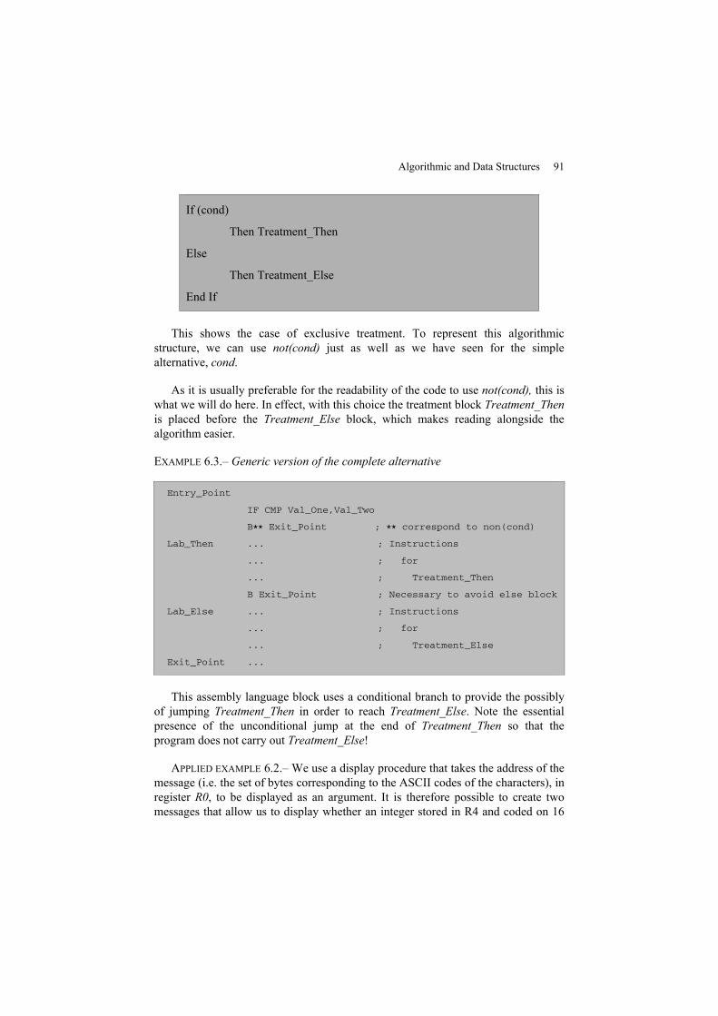
Algorithmic and Data Structures 91
If (cond)
Then Treatment_Then
Else
Then Treatment_Else
End If
This shows the case of exclusive treatment. To represent this algorithmicstructure, we can use not(cond) just as well as we have seen for the simplealternative, cond.
As it is usually preferable for the readability of the code to use not(cond), this iswhat we will do here. In effect, with this choice the treatment block Treatment_Thenis placed before the Treatment_Else block, which makes reading alongside thealgorithm easier.
EXAMPLE 6.3.– Generic version of the complete alternative
Entry_Point
IF CMP Val_One,Val_Two
B⋆⋆ Exit_Point ; ⋆⋆ correspond to non(cond)
Lab_Then ... ; Instructions
... ; for
... ; Treatment_Then
B Exit_Point ; Necessary to avoid else block
Lab_Else ... ; Instructions
... ; for
... ; Treatment_Else
Exit_Point ...
This assembly language block uses a conditional branch to provide the possiblyof jumping Treatment_Then in order to reach Treatment_Else. Note the essentialpresence of the unconditional jump at the end of Treatment_Then so that theprogram does not carry out Treatment_Else!
APPLIED EXAMPLE 6.2.– We use a display procedure that takes the address of themessage (i.e. the set of bytes corresponding to the ASCII codes of the characters), inregister R0, to be displayed as an argument. It is therefore possible to create twomessages that allow us to display whether an integer stored in R4 and coded on 16
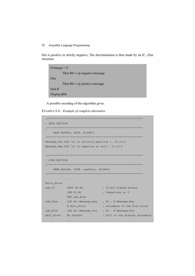
92 Assembly Language Programming
bits is positive or strictly negative. The discrimination is then made by an If…Elsestructure:
If Integer < 0Then R0←@ negative message
ElseThen R0←@ positive message
End IfDisplay(R0)
A possible encoding of this algorithm gives:
EXAMPLE 6.4.– Example of complete alternative
;*************************************************************
; DATA SECTION
;*************************************************************
AREA MyDATA, DATA, ALIGN=0
;*************************************************************
Message_Pos DCB "It is strictly positive ", 10,13,0
Message_Neg DCB "It is negative or null", 10,13,0
;*************************************************************
; CODE SECTION
;*************************************************************
AREA MyCode, CODE, readonly, ALIGN=2
;*************************************************************
...
Entry_Point
Lab_If SXHT R3,R4 ; 32-bit signed extend
CMP R3,#0 ; Comparison at 0
BGT,Lab_Else
Lab_Then LDR R0,=Message_Neg ; R0 ← @ Message_Neg
B Exit_Point ; Avoidance of the Else block
Lab_Else LDR R0,=Message_Pos ; R0 ← @ Message_Pos
Exit_Point BL DispStr ; Call to the display procedure
...
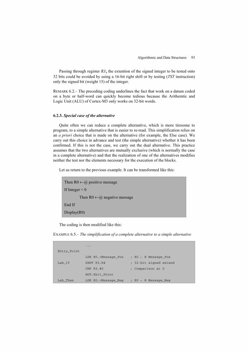
Algorithmic and Data Structures 93
Passing through register R3, the extention of the signed integer to be tested onto32 bits could be avoided by using a 16-bit right shift or by testing (TST instruction)only the signed bit (weight 15) of the integer.
REMARK 6.2.– The preceding coding underlines the fact that work on a datum codedon a byte or half-word can quickly become tedious because the Arithemtic andLogic Unit (ALU) of Cortex-M3 only works on 32-bit words.
6.2.3. Special case of the alternative
Quite often we can reduce a complete alternative, which is more tiresome toprogram, to a simple alternative that is easier to re-read. This simplification relies onan a priori choice that is made on the alternative (for example, the Else case). Wecarry out this choice in advance and test (the simple alternative) whether it has beenconfirmed. If this is not the case, we carry out the dual alternative. This practiceassumes that the two alternatives are mutually exclusive (which is normally the casein a complete alternative) and that the realization of one of the alternatives modifiesneither the test nor the elements necessary for the execution of the blocks.
Let us return to the previous example. It can be transformed like this:
Then R0←@ positive message
If Integer < 0
Then R0←@ negative message
End If
Display(R0)
The coding is then modified like this:
EXAMPLE 6.5.– The simplification of a complete alternative to a simple alternative
...
Entry_Point
LDR R0,=Message_Pos ; R0 ← @ Message_Pos
Lab_If SXHT R3,R4 ; 32-bit signed extend
CMP R3,#0 ; Comparison at 0
BGT,Exit_Point
Lab_Then LDR R0,=Message_Neg ; R0 ← @ Message_Neg
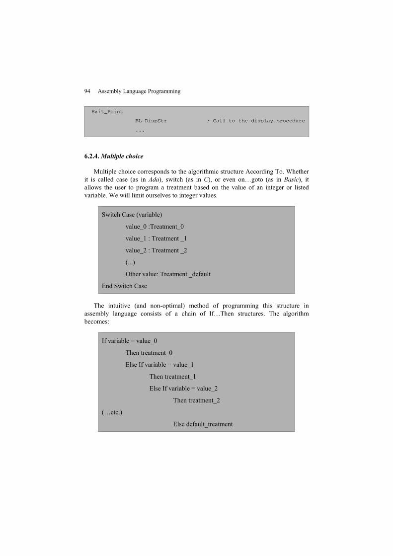
94 Assembly Language Programming
Exit_Point
BL DispStr ; Call to the display procedure
...
6.2.4.Multiple choice
Multiple choice corresponds to the algorithmic structure According To. Whetherit is called case (as in Ada), switch (as in C), or even on…goto (as in Basic), itallows the user to program a treatment based on the value of an integer or listedvariable. We will limit ourselves to integer values.
Switch Case (variable)
value_0 :Treatment_0
value_1 : Treatment _1
value_2 : Treatment _2
(...)
Other value: Treatment _default
End Switch Case
The intuitive (and non-optimal) method of programming this structure inassembly language consists of a chain of If…Then structures. The algorithmbecomes:
If variable = value_0
Then treatment_0
Else If variable = value_1
Then treatment_1
Else If variable = value_2
Then treatment_2
(…etc.)
Else default_treatment
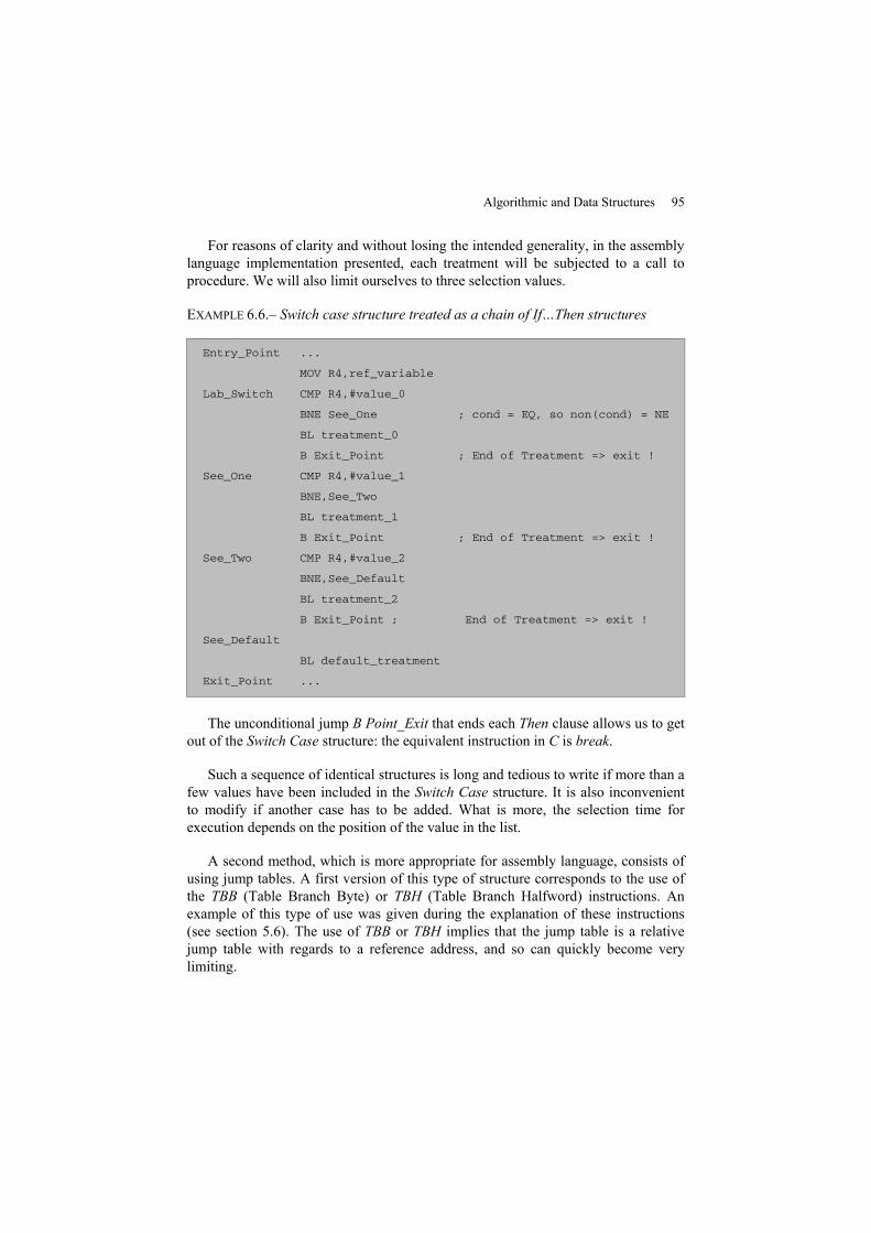
Algorithmic and Data Structures 95
For reasons of clarity and without losing the intended generality, in the assemblylanguage implementation presented, each treatment will be subjected to a call toprocedure. We will also limit ourselves to three selection values.
EXAMPLE 6.6.– Switch case structure treated as a chain of If…Then structures
Entry_Point ...
MOV R4,ref_variable
Lab_Switch CMP R4,#value_0
BNE See_One ; cond = EQ, so non(cond) = NE
BL treatment_0
B Exit_Point ; End of Treatment => exit !
See_One CMP R4,#value_1
BNE,See_Two
BL treatment_1
B Exit_Point ; End of Treatment => exit !
See_Two CMP R4,#value_2
BNE,See_Default
BL treatment_2
B Exit_Point ; End of Treatment => exit !
See_Default
BL default_treatment
Exit_Point ...
The unconditional jump B Point_Exit that ends each Then clause allows us to getout of the Switch Case structure: the equivalent instruction in C is break.
Such a sequence of identical structures is long and tedious to write if more than afew values have been included in the Switch Case structure. It is also inconvenientto modify if another case has to be added. What is more, the selection time forexecution depends on the position of the value in the list.
A second method, which is more appropriate for assembly language, consists ofusing jump tables. A first version of this type of structure corresponds to the use ofthe TBB (Table Branch Byte) or TBH (Table Branch Halfword) instructions. Anexample of this type of use was given during the explanation of these instructions(see section 5.6). The use of TBB or TBH implies that the jump table is a relativejump table with regards to a reference address, and so can quickly become verylimiting.
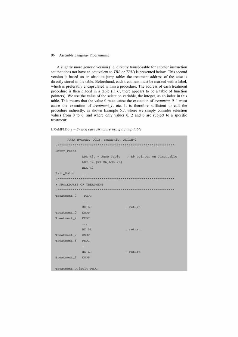
96 Assembly Language Programming
A slightly more generic version (i.e. directly transposable for another instructionset that does not have an equivalent to TBB or TBH) is presented below. This secondversion is based on an absolute jump table: the treatment address of the case isdirectly stored in the table. Beforehand, each treatment must be marked with a label,which is preferably encapsulated within a procedure. The address of each treatmentprocedure is then placed in a table (in C, there appears to be a table of functionpointers). We use the value of the selection variable, the integer, as an index in thistable. This means that the value 0 must cause the execution of treatment_0, 1 mustcause the execution of treatment_1, etc. It is therefore sufficient to call theprocedure indirectly, as shown Example 6.7, where we simply consider selectionvalues from 0 to 6, and where only values 0, 2 and 6 are subject to a specifictreatment:
EXAMPLE 6.7.– Switch case structure using a jump table
AREA MyCode, CODE, readonly, ALIGN=2
;*************************************************************
Entry_Point
LDR R9, = Jump Table ; R9 pointer on Jump_table
LDR R2,[R9,R6,LSL #2]
BLX R2
Exit_Point ...
;*************************************************************
; PROCEDURES OF TREATMENT
;*************************************************************
Treatment_0 PROC
...
BX LR ; return
Treatment_0 ENDP
Treatment_2 PROC
...
BX LR ; return
Treatment_2 ENDP
Treatment_6 PROC
...
BX LR ; return
Treatment_6 ENDP
Treatment_Default PROC
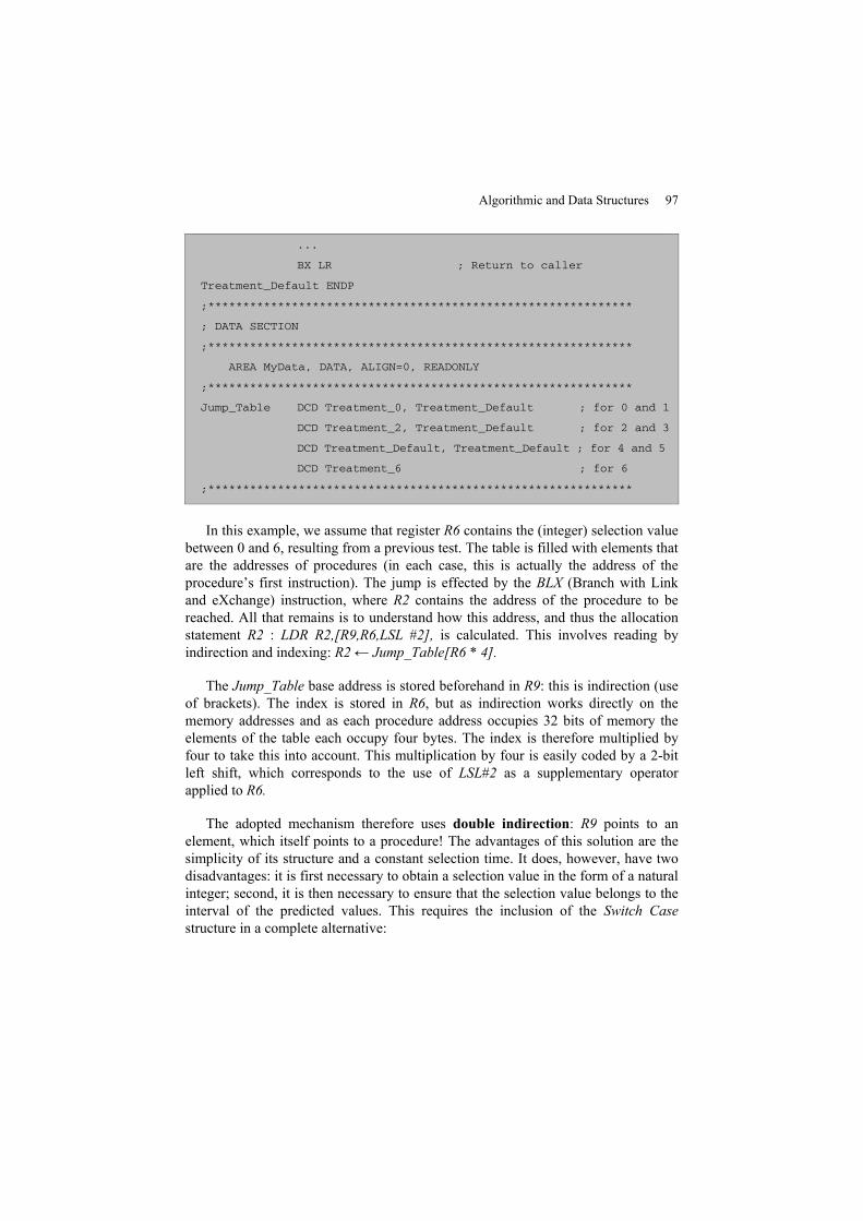
Algorithmic and Data Structures 97
...
BX LR ; Return to caller
Treatment_Default ENDP
;*************************************************************
; DATA SECTION
;*************************************************************
AREA MyData, DATA, ALIGN=0, READONLY
;*************************************************************
Jump_Table DCD Treatment_0, Treatment_Default ; for 0 and 1
DCD Treatment_2, Treatment_Default ; for 2 and 3
DCD Treatment_Default, Treatment_Default ; for 4 and 5
DCD Treatment_6 ; for 6
;*************************************************************
In this example, we assume that register R6 contains the (integer) selection valuebetween 0 and 6, resulting from a previous test. The table is filled with elements thatare the addresses of procedures (in each case, this is actually the address of theprocedure’s first instruction). The jump is effected by the BLX (Branch with Linkand eXchange) instruction, where R2 contains the address of the procedure to bereached. All that remains is to understand how this address, and thus the allocationstatement R2 : LDR R2,[R9,R6,LSL #2], is calculated. This involves reading byindirection and indexing: R2← Jump_Table[R6 * 4].
The Jump_Table base address is stored beforehand in R9: this is indirection (useof brackets). The index is stored in R6, but as indirection works directly on thememory addresses and as each procedure address occupies 32 bits of memory theelements of the table each occupy four bytes. The index is therefore multiplied byfour to take this into account. This multiplication by four is easily coded by a 2-bitleft shift, which corresponds to the use of LSL#2 as a supplementary operatorapplied to R6.
The adopted mechanism therefore uses double indirection: R9 points to anelement, which itself points to a procedure! The advantages of this solution are thesimplicity of its structure and a constant selection time. It does, however, have twodisadvantages: it is first necessary to obtain a selection value in the form of a naturalinteger; second, it is then necessary to ensure that the selection value belongs to theinterval of the predicted values. This requires the inclusion of the Switch Casestructure in a complete alternative:
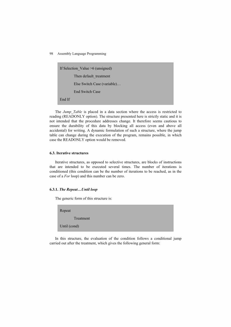
98 Assembly Language Programming
If Selection_Value >6 (unsigned)
Then default_treatment
Else Switch Case (variable)…
End Switch Case
End If
The Jump_Table is placed in a data section where the access is restricted toreading (READONLY option). The structure presented here is strictly static and it isnot intended that the procedure addresses change. It therefore seems cautious toensure the durability of this data by blocking all access (even and above allaccidental) for writing. A dynamic formulation of such a structure, where the jumptable can change during the execution of the program, remains possible, in whichcase the READONLY option would be removed.
6.3. Iterative structures
Iterative structures, as opposed to selective structures, are blocks of instructionsthat are intended to be executed several times. The number of iterations isconditioned (this condition can be the number of iterations to be reached, as in thecase of a For loop) and this number can be zero.
6.3.1. The Repeat…Until loop
The generic form of this structure is:
Repeat
Treatment
Until (cond)
In this structure, the evaluation of the condition follows a conditional jumpcarried out after the treatment, which gives the following general form:
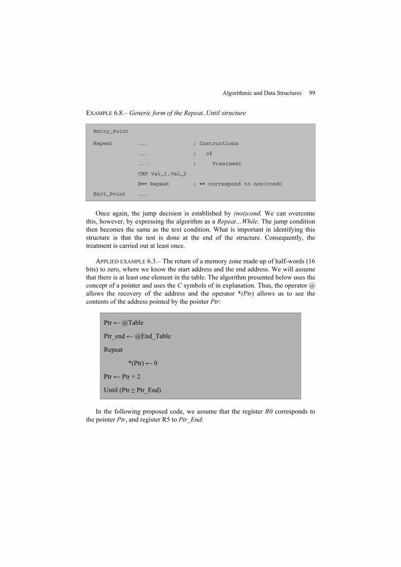
Algorithmic and Data Structures 99
EXAMPLE 6.8.– Generic form of the Repeat..Until structure
Entry_Point
Repeat ... ; Instructions
... ; of
... ; Treatment
CMP Val_1,Val_2
B⋆⋆ Repeat ; ⋆⋆ correspond to non(cond)
Exit_Point ...
Once again, the jump decision is established by (not)cond. We can overcomethis, however, by expressing the algorithm as a Repeat…While. The jump conditionthen becomes the same as the text condition. What is important in identifying thisstructure is that the test is done at the end of the structure. Consequently, thetreatment is carried out at least once.
APPLIED EXAMPLE 6.3.– The return of a memory zone made up of half-words (16bits) to zero, where we know the start address and the end address. We will assumethat there is at least one element in the table. The algorithm presented below uses theconcept of a pointer and uses the C symbols of in explanation. Thus, the operator @allows the recovery of the address and the operator *(Ptr) allows us to see thecontents of the address pointed by the pointer Ptr:
Ptr←@Table
Ptr_end←@End_Table
Repeat
*(Ptr)← 0
Ptr← Ptr + 2
Until (Ptr ≥ Ptr_End)
In the following proposed code, we assume that the register R0 corresponds tothe pointer Ptr, and register R5 to Ptr_End:
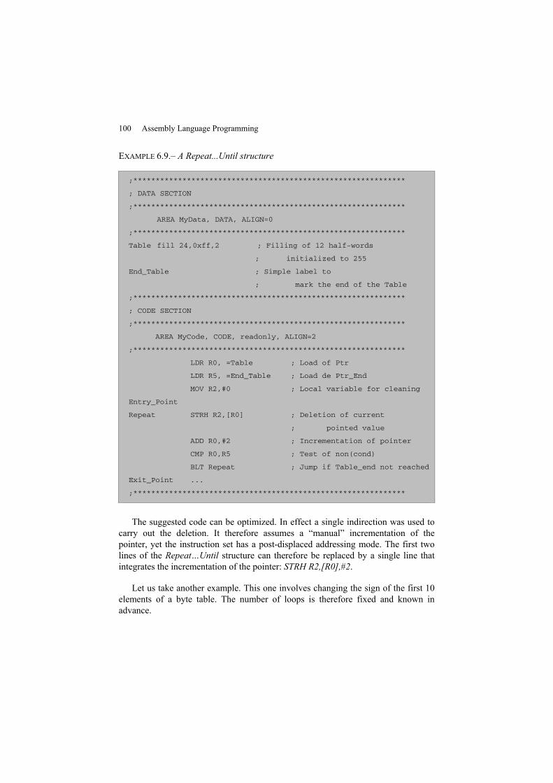
100 Assembly Language Programming
EXAMPLE 6.9.– A Repeat...Until structure
;*************************************************************
; DATA SECTION
;*************************************************************
AREA MyData, DATA, ALIGN=0
;*************************************************************
Table fill 24,0xff,2 ; Filling of 12 half-words
; initialized to 255
End_Table ; Simple label to
; mark the end of the Table
;*************************************************************
; CODE SECTION
;*************************************************************
AREA MyCode, CODE, readonly, ALIGN=2
;*************************************************************
LDR R0, =Table ; Load of Ptr
LDR R5, =End_Table ; Load de Ptr_End
MOV R2,#0 ; Local variable for cleaning
Entry_Point
Repeat STRH R2,[R0] ; Deletion of current
; pointed value
ADD R0,#2 ; Incrementation of pointer
CMP R0,R5 ; Test of non(cond)
BLT Repeat ; Jump if Table_end not reached
Exit_Point ...
;*************************************************************
The suggested code can be optimized. In effect a single indirection was used tocarry out the deletion. It therefore assumes a “manual” incrementation of thepointer, yet the instruction set has a post-displaced addressing mode. The first twolines of the Repeat…Until structure can therefore be replaced by a single line thatintegrates the incrementation of the pointer: STRH R2,[R0],#2.
Let us take another example. This one involves changing the sign of the first 10elements of a byte table. The number of loops is therefore fixed and known inadvance.
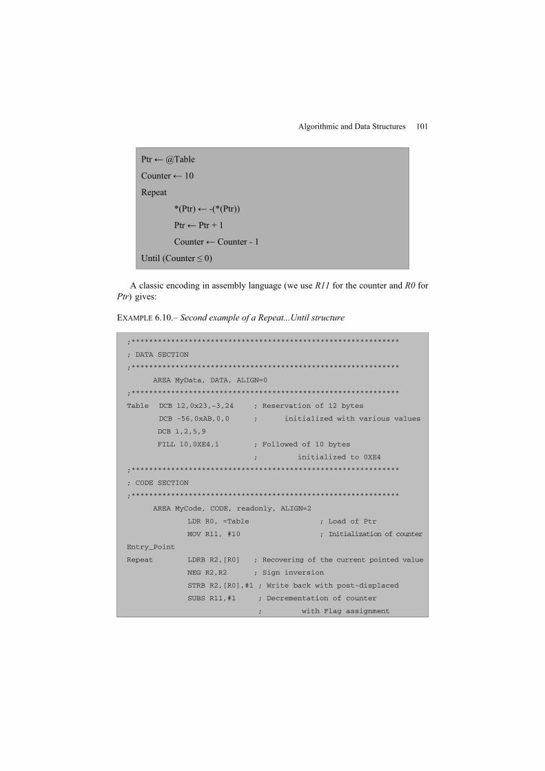
Algorithmic and Data Structures 101
Ptr←@Table
Counter← 10
Repeat
*(Ptr)← -(*(Ptr))
Ptr← Ptr + 1
Counter← Counter - 1
Until (Counter ≤ 0)
A classic encoding in assembly language (we use R11 for the counter and R0 forPtr) gives:
EXAMPLE 6.10.– Second example of a Repeat...Until structure
;*************************************************************
; DATA SECTION
;*************************************************************
AREA MyData, DATA, ALIGN=0
;*************************************************************
Table DCB 12,0x23,-3,24 ; Reservation of 12 bytes
DCB -56,0xAB,0,0 ; initialized with various values
DCB 1,2,5,9
FILL 10,0XE4,1 ; Followed of 10 bytes
; initialized to 0XE4
;*************************************************************
; CODE SECTION
;*************************************************************
AREA MyCode, CODE, readonly, ALIGN=2
LDR R0, =Table ; Load of Ptr
MOV R11, #10 ; Initialization of counter
Entry_Point
Repeat LDRB R2,[R0] ; Recovering of the current pointed value
NEG R2,R2 ; Sign inversion
STRB R2,[R0],#1 ; Write back with post-displaced
SUBS R11,#1 ; Decrementation of counter
; with Flag assignment
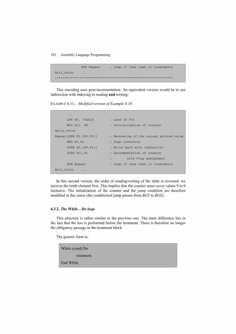
102 Assembly Language Programming
BGT Repeat ; Jump if less than 10 treatments
Exit_Point ...
;*************************************************************
This encoding uses post-incrementation. An equivalent version would be to useindirection with indexing in reading and writing:
EXAMPLE 6.11.–Modified version of Example 6.10
...
LDR R0, =Table ; Load of Ptr
MOV R11, #9 ; Initialization of counter
Entry_Point
Repeat LDRB R2,[R0,R11] ; Recovering of the current pointed value
NEG R2,R2 ; Sign inversion
STRB R2,[R0,R11] ; Write back with indexation
SUBS R11,#1 ; Decrementation of counter
; with Flag assignment
BGE Repeat ; Jump if less than 10 treatments
Exit_Point ...
In this second version, the order of reading/writing of the table is reversed: werecover the tenth element first. This implies that the counter must cover values 9 to 0inclusive. The initialization of the counter and the jump condition are thereforemodified in this sense (the conditioned jump passes from BGT to BGE).
6.3.2. The While…Do loop
This structure is rather similar to the previous one. The main difference lies inthe fact that the test is performed before the treatment. There is therefore no longerthe obligatory passage in the treatment block.
The generic form is:
While (cond) Do
treatment
End While
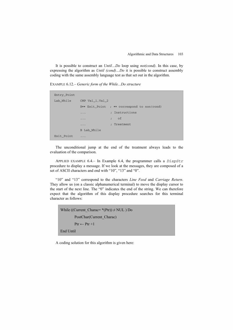
Algorithmic and Data Structures 103
It is possible to construct an Until…Do loop using not(cond). In this case, byexpressing the algorithm as Until (cond)…Do it is possible to construct assemblycoding with the same assembly language test as that set out in the algorithm.
EXAMPLE 6.12.– Generic form of the While...Do structure
Entry_Point
Lab_While CMP Val_1,Val_2
B⋆⋆ Exit_Point ; ⋆⋆ correspond to non(cond)
... ; Instructions
... ; of
... ; Treatment
B Lab_While
Exit_Point ...
The unconditional jump at the end of the treatment always leads to theevaluation of the comparison.
APPLIED EXAMPLE 6.4.– In Example 6.4, the programmer calls a DispStrprocedure to display a message. If we look at the messages, they are composed of aset of ASCII characters and end with “10”, “13” and “0”.
“10” and “13” correspond to the characters Line Feed and Carriage Return.They allow us (on a classic alphanumerical terminal) to move the display cursor tothe start of the next line. The “0” indicates the end of the string. We can thereforeexpect that the algorithm of this display procedure searches for this terminalcharacter as follows:
While ((Current_Charac= *(Ptr)) ≠ NUL ) Do
PostChar(Current_Charac)
Ptr← Ptr +1
End Until
A coding solution for this algorithm is given here:
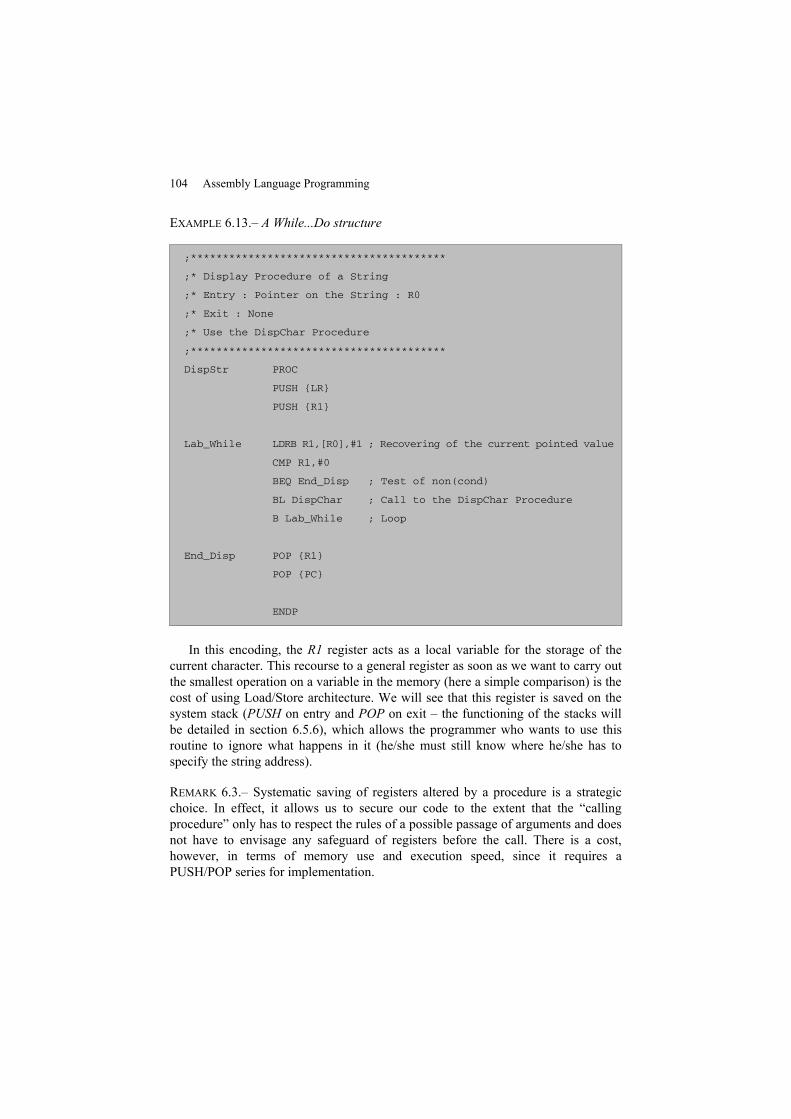
104 Assembly Language Programming
EXAMPLE 6.13.– A While...Do structure
;****************************************
;* Display Procedure of a String
;* Entry : Pointer on the String : R0
;* Exit : None
;* Use the DispChar Procedure
;****************************************
DispStr PROC
PUSH {LR}
PUSH {R1}
Lab_While LDRB R1,[R0],#1 ; Recovering of the current pointed value
CMP R1,#0
BEQ End_Disp ; Test of non(cond)
BL DispChar ; Call to the DispChar Procedure
B Lab_While ; Loop
End_Disp POP {R1}
POP {PC}
ENDP
In this encoding, the R1 register acts as a local variable for the storage of thecurrent character. This recourse to a general register as soon as we want to carry outthe smallest operation on a variable in the memory (here a simple comparison) is thecost of using Load/Store architecture. We will see that this register is saved on thesystem stack (PUSH on entry and POP on exit – the functioning of the stacks willbe detailed in section 6.5.6), which allows the programmer who wants to use thisroutine to ignore what happens in it (he/she must still know where he/she has tospecify the string address).
REMARK 6.3.– Systematic saving of registers altered by a procedure is a strategicchoice. In effect, it allows us to secure our code to the extent that the “callingprocedure” only has to respect the rules of a possible passage of arguments and doesnot have to envisage any safeguard of registers before the call. There is a cost,however, in terms of memory use and execution speed, since it requires aPUSH/POP series for implementation.
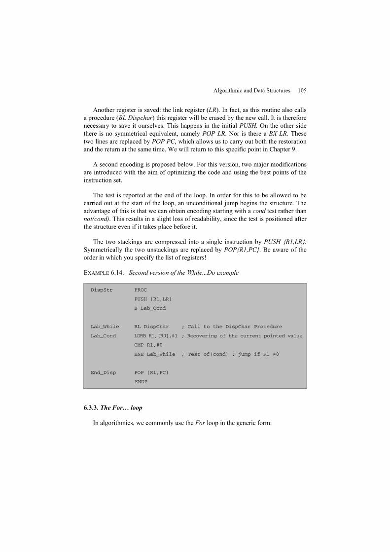
Algorithmic and Data Structures 105
Another register is saved: the link register (LR). In fact, as this routine also callsa procedure (BL Dispchar) this register will be erased by the new call. It is thereforenecessary to save it ourselves. This happens in the initial PUSH. On the other sidethere is no symmetrical equivalent, namely POP LR. Nor is there a BX LR. Thesetwo lines are replaced by POP PC, which allows us to carry out both the restorationand the return at the same time. We will return to this specific point in Chapter 9.
A second encoding is proposed below. For this version, two major modificationsare introduced with the aim of optimizing the code and using the best points of theinstruction set.
The test is reported at the end of the loop. In order for this to be allowed to becarried out at the start of the loop, an unconditional jump begins the structure. Theadvantage of this is that we can obtain encoding starting with a cond test rather thannot(cond). This results in a slight loss of readability, since the test is positioned afterthe structure even if it takes place before it.
The two stackings are compressed into a single instruction by PUSH {R1,LR}.Symmetrically the two unstackings are replaced by POP{R1,PC}. Be aware of theorder in which you specify the list of registers!
EXAMPLE 6.14.– Second version of the While...Do example
DispStr PROC
PUSH {R1,LR}
B Lab_Cond
Lab_While BL DispChar ; Call to the DispChar Procedure
Lab_Cond LDRB R1,[R0],#1 ; Recovering of the current pointed value
CMP R1,#0
BNE Lab_While ; Test of(cond) : jump if R1 ≠0
End_Disp POP {R1,PC}
ENDP
6.3.3. The For… loop
In algorithmics, we commonly use the For loop in the generic form:
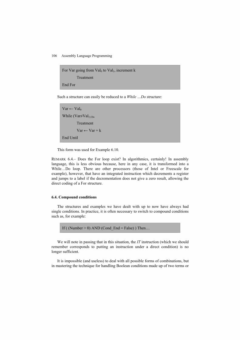
106 Assembly Language Programming
For Var going from Val0 to Val1, increment k
Treatment
End For
Such a structure can easily be reduced to aWhile …Do structure:
Var← Val0
While (Var≠Val1) Do
Treatment
Var← Var + k
End Until
This form was used for Example 6.10.
REMARK 6.4.– Does the For loop exist? In algorithmics, certainly! In assemblylanguage, this is less obvious because, here in any case, it is transformed into aWhile…Do loop. There are other processors (those of Intel or Freescale forexample), however, that have an integrated instruction which decrements a registerand jumps to a label if the decrementation does not give a zero result, allowing thedirect coding of a For structure.
6.4. Compound conditions
The structures and examples we have dealt with up to now have always hadsingle conditions. In practice, it is often necessary to switch to compound conditionssuch as, for example:
If ( (Number > 0) AND (Cond_End = False) ) Then…
We will note in passing that in this situation, the IT instruction (which we shouldremember corresponds to putting an instruction under a direct condition) is nolonger sufficient.
It is impossible (and useless) to deal with all possible forms of combinations, butin mastering the technique for handling Boolean conditions made up of two terms or
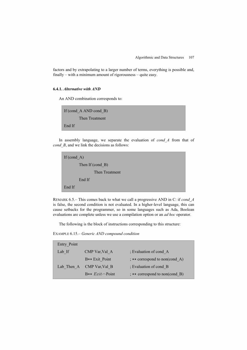
Algorithmic and Data Structures 107
factors and by extrapolating to a larger number of terms, everything is possible and,finally – with a minimum amount of rigorousness – quite easy.
6.4.1. Alternative with AND
An AND combination corresponds to:
If (cond_A AND cond_B)
Then Treatment
End If
In assembly language, we separate the evaluation of cond_A from that ofcond_B, and we link the decisions as follows:
If (cond_A)
Then If (cond_B)
Then Treatment
End If
End If
REMARK 6.5.– This comes back to what we call a progressive AND in C: if cond_Ais false, the second condition is not evaluated. In a higher-level language, this cancause setbacks for the programmer, so in some languages such as Ada, Booleanevaluations are complete unless we use a compilation option or an ad hoc operator.
The following is the block of instructions corresponding to this structure:
EXAMPLE 6.15.– Generic AND compound condition
Entry_Point
Lab_If CMP Var,Val_A ; Evaluation of cond_A
B⋆⋆ Exit_Point ; ⋆⋆ correspond to non(cond_A)Lab_Then_A CMP Var,Val_B ; Evaluation of cond_B
B⋆⋆ Exit_Point ; ⋆⋆ correspond to non(cond_B)
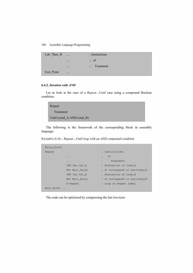
108 Assembly Language Programming
Lab_Then_B ... ; Instructions
... ; of
... ; Treatment
Exit_Point ...
6.4.2. Iteration with AND
Let us look at the case of a Repeat…Until case using a compound Booleancondition.
Repeat
Treatment
Until (cond_A AND cond_B)
The following is the framework of the corresponding block in assemblylanguage:
EXAMPLE 6.16.– Repeat…Until loop with an AND compound condition
Entry_Point
Repeat ; Instructions
... ; of
... ; Treatment
CMP Var,Val_A ; Evaluation of cond_A
B⋆⋆ Exit_Point ; ⋆⋆ correspond to non(cond_A)
CMP Var,Val_B ; Evaluation of cond_B
B⋆⋆ Exit_Point ; ⋆⋆ correspond to non(cond_B)
B Repeat ; Loop on Repeat Label
Exit_Point ...
The code can be optimized by compressing the last two tests:
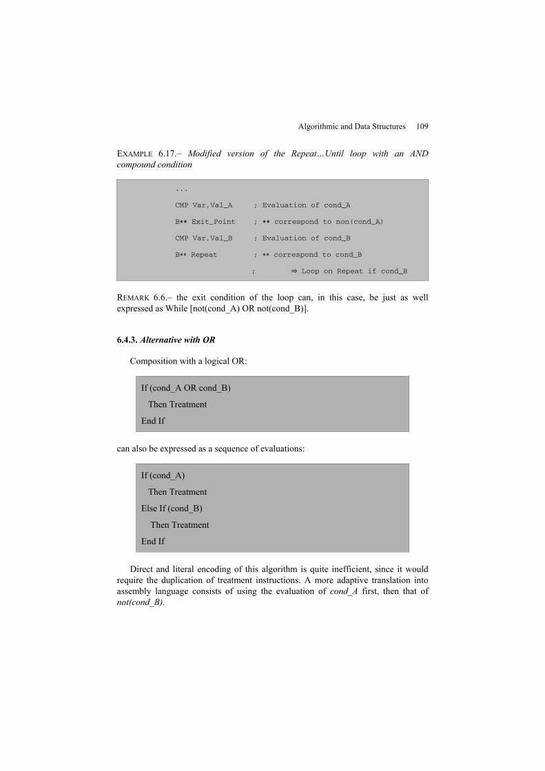
Algorithmic and Data Structures 109
EXAMPLE 6.17.– Modified version of the Repeat…Until loop with an ANDcompound condition
...
CMP Var,Val_A ; Evaluation of cond_A
B⋆⋆ Exit_Point ; ⋆⋆ correspond to non(cond_A)
CMP Var,Val_B ; Evaluation of cond_B
B∗∗ Repeat ; ∗∗ correspond to cond_B
; ⇒ Loop on Repeat if cond_B
REMARK 6.6.– the exit condition of the loop can, in this case, be just as wellexpressed as While [not(cond_A) OR not(cond_B)].
6.4.3. Alternative with OR
Composition with a logical OR:
If (cond_A OR cond_B)
Then Treatment
End If
can also be expressed as a sequence of evaluations:
If (cond_A)
Then Treatment
Else If (cond_B)
Then Treatment
End If
Direct and literal encoding of this algorithm is quite inefficient, since it wouldrequire the duplication of treatment instructions. A more adaptive translation intoassembly language consists of using the evaluation of cond_A first, then that ofnot(cond_B).
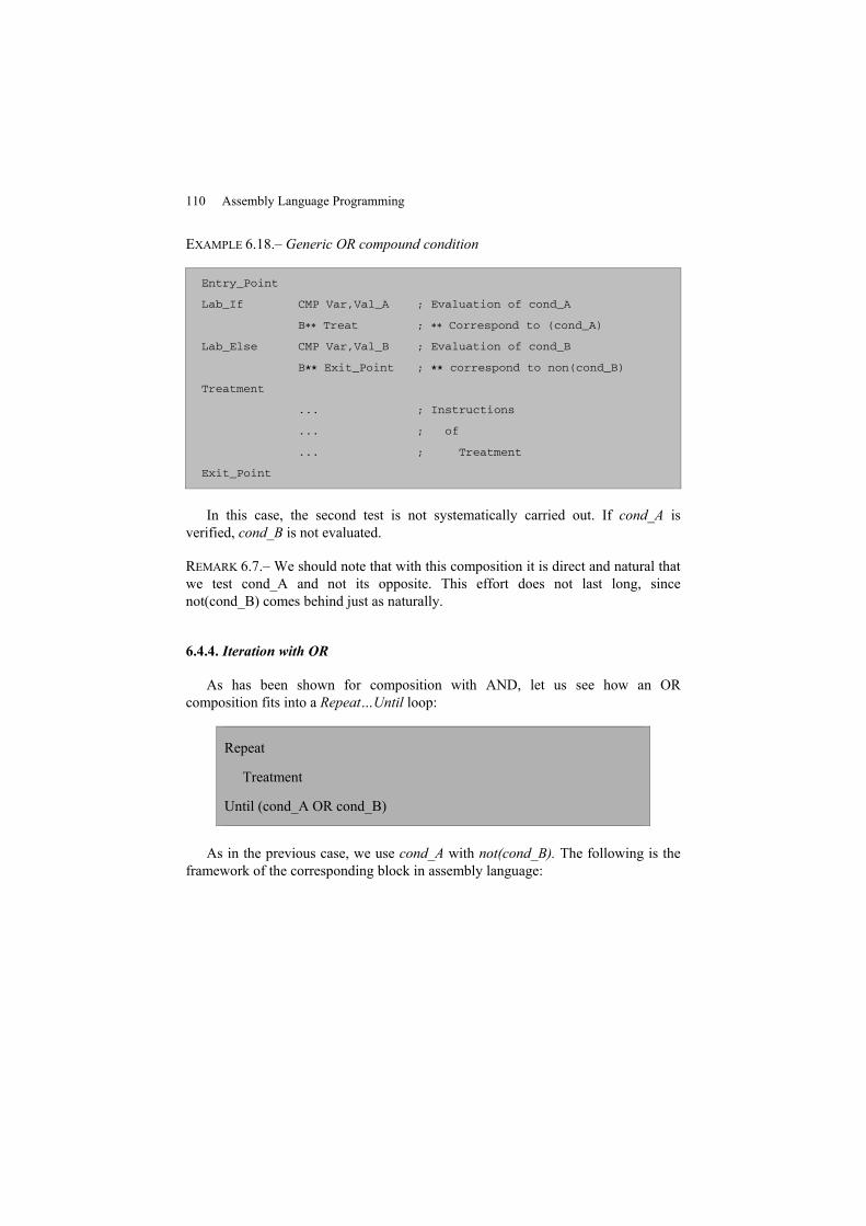
110 Assembly Language Programming
EXAMPLE 6.18.– Generic OR compound condition
Entry_Point
Lab_If CMP Var,Val_A ; Evaluation of cond_A
B∗∗ Treat ; ∗∗ Correspond to (cond_A)
Lab_Else CMP Var,Val_B ; Evaluation of cond_B
B⋆⋆ Exit_Point ; ⋆⋆ correspond to non(cond_B)
Treatment
... ; Instructions
... ; of
... ; Treatment
Exit_Point
In this case, the second test is not systematically carried out. If cond_A isverified, cond_B is not evaluated.
REMARK 6.7.– We should note that with this composition it is direct and natural thatwe test cond_A and not its opposite. This effort does not last long, sincenot(cond_B) comes behind just as naturally.
6.4.4. Iteration with OR
As has been shown for composition with AND, let us see how an ORcomposition fits into a Repeat…Until loop:
Repeat
Treatment
Until (cond_A OR cond_B)
As in the previous case, we use cond_A with not(cond_B). The following is theframework of the corresponding block in assembly language:
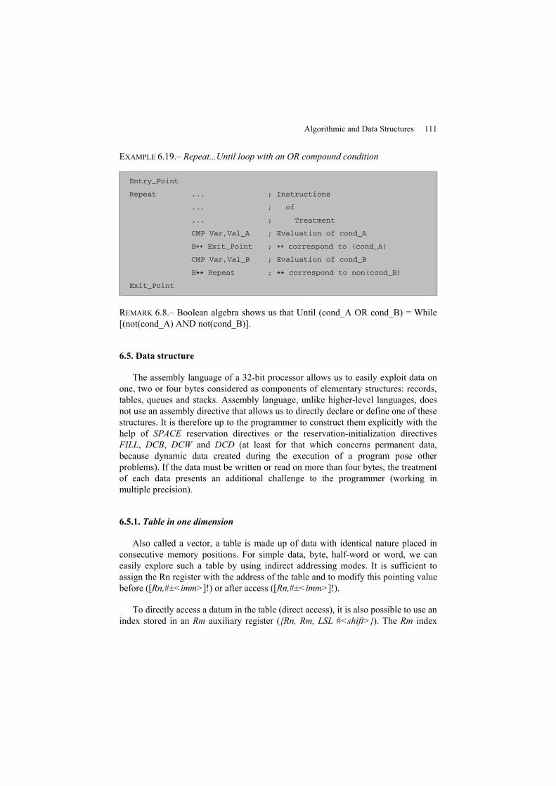
Algorithmic and Data Structures 111
EXAMPLE 6.19.– Repeat...Until loop with an OR compound condition
Entry_Point
Repeat ... ; Instructions
... ; of
... ; Treatment
CMP Var,Val_A ; Evaluation of cond_A
B∗∗ Exit_Point ; ∗∗ correspond to (cond_A)
CMP Var,Val_B ; Evaluation of cond_B
B⋆⋆ Repeat ; ⋆⋆ correspond to non(cond_B)
Exit_Point
REMARK 6.8.– Boolean algebra shows us that Until (cond_A OR cond_B) = While[(not(cond_A) AND not(cond_B)].
6.5. Data structure
The assembly language of a 32-bit processor allows us to easily exploit data onone, two or four bytes considered as components of elementary structures: records,tables, queues and stacks. Assembly language, unlike higher-level languages, doesnot use an assembly directive that allows us to directly declare or define one of thesestructures. It is therefore up to the programmer to construct them explicitly with thehelp of SPACE reservation directives or the reservation-initialization directivesFILL, DCB, DCW and DCD (at least for that which concerns permanent data,because dynamic data created during the execution of a program pose otherproblems). If the data must be written or read on more than four bytes, the treatmentof each data presents an additional challenge to the programmer (working inmultiple precision).
6.5.1. Table in one dimension
Also called a vector, a table is made up of data with identical nature placed inconsecutive memory positions. For simple data, byte, half-word or word, we caneasily explore such a table by using indirect addressing modes. It is sufficient toassign the Rn register with the address of the table and to modify this pointing valuebefore ([Rn,#±<imm>]!) or after access ([Rn,#±<imm>]!).
To directly access a datum in the table (direct access), it is also possible to use anindex stored in an Rm auxiliary register ({Rn, Rm, LSL #<shift>}). The Rm index
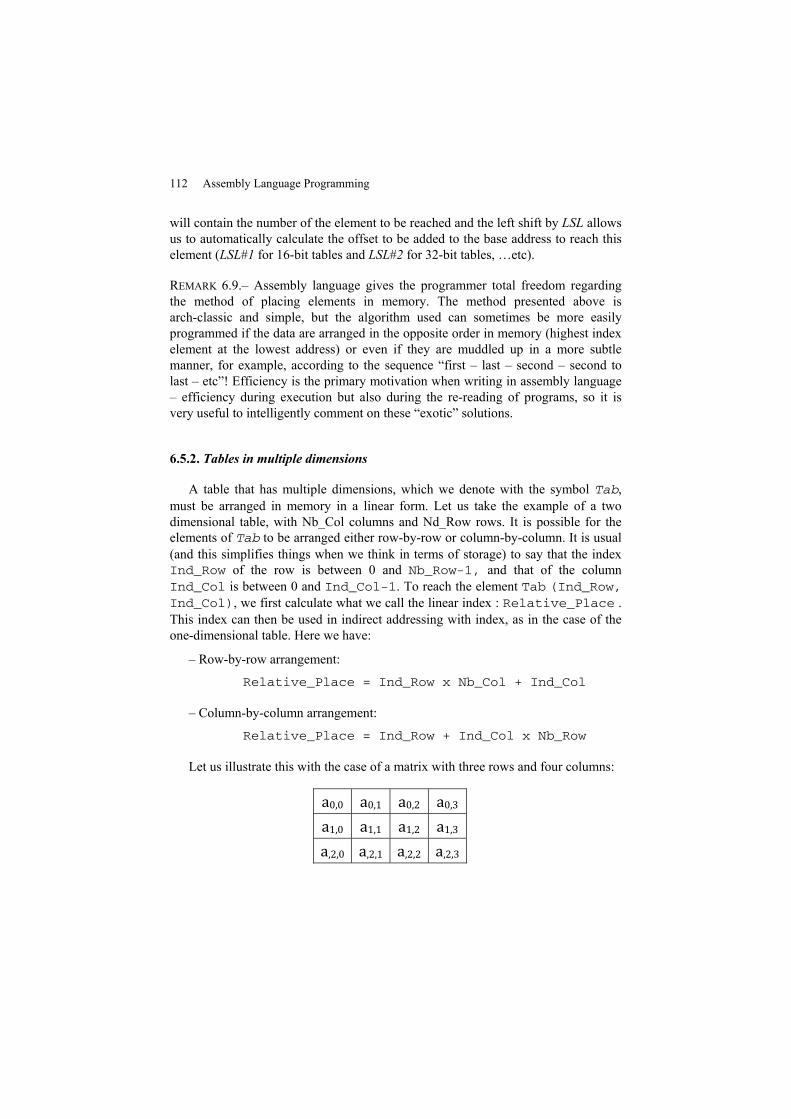
112 Assembly Language Programming
will contain the number of the element to be reached and the left shift by LSL allowsus to automatically calculate the offset to be added to the base address to reach thiselement (LSL#1 for 16-bit tables and LSL#2 for 32-bit tables, …etc).
REMARK 6.9.– Assembly language gives the programmer total freedom regardingthe method of placing elements in memory. The method presented above isarch-classic and simple, but the algorithm used can sometimes be more easilyprogrammed if the data are arranged in the opposite order in memory (highest indexelement at the lowest address) or even if they are muddled up in a more subtlemanner, for example, according to the sequence “first – last – second – second tolast – etc”! Efficiency is the primary motivation when writing in assembly language– efficiency during execution but also during the re-reading of programs, so it isvery useful to intelligently comment on these “exotic” solutions.
6.5.2. Tables in multiple dimensions
A table that has multiple dimensions, which we denote with the symbol Tab,must be arranged in memory in a linear form. Let us take the example of a twodimensional table, with Nb_Col columns and Nd_Row rows. It is possible for theelements of Tab to be arranged either row-by-row or column-by-column. It is usual(and this simplifies things when we think in terms of storage) to say that the indexInd_Row of the row is between 0 and Nb_Row-1, and that of the columnInd_Col is between 0 and Ind_Col-1. To reach the element Tab (Ind_Row,Ind_Col), we first calculate what we call the linear index : Relative_Place .This index can then be used in indirect addressing with index, as in the case of theone-dimensional table. Here we have:
– Row-by-row arrangement:
Relative_Place = Ind_Row x Nb_Col + Ind_Col
– Column-by-column arrangement:
Relative_Place = Ind_Row + Ind_Col x Nb_Row
Let us illustrate this with the case of a matrix with three rows and four columns:a0,0 a0,1 a0,2 a0,3a1,0 a1,1 a1,2 a1,3a,2,0 a,2,1 a,2,2 a,2,3
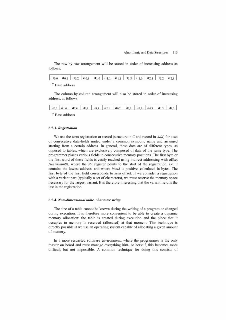
Algorithmic and Data Structures 113
The row-by-row arrangement will be stored in order of increasing address asfollows:a0,0 a0,1 a0,2 a0,3 a1,0 a1,1 a1,2 a1,3 a2,0 a2,1 a2,2 a2,3↑ Base address
The column-by-column arrangement will also be stored in order of increasingaddress, as follows:a0,0 a1,0 a2,0 a0,1 a1,1 a2,1 a0,2 a1,2 a2,2 a0,3 a1,3 a2,3↑ Base address
6.5.3. Registration
We use the term registration or record (structure in C and record in Ada) for a setof consecutive data-fields united under a common symbolic name and arrangedstarting from a certain address. In general, these data are of different types, asopposed to tables, which are exclusively composed of data of the same type. Theprogrammer places various fields in consecutive memory positions. The first byte orthe first word of these fields is easily reached using indirect addressing with offset[Rn+#imm8], where the Rn register points to the start of the registration, i.e. itcontains the lowest address, and where imm8 is positive, calculated in bytes. Thefirst byte of the first field corresponds to zero offset. If we consider a registrationwith a variant part (typically a set of characters), we must reserve the memory spacenecessary for the largest variant. It is therefore interesting that the variant field is thelast in the registration.
6.5.4. Non-dimensional table, character string
The size of a table cannot be known during the writing of a program or changedduring execution. It is therefore more convenient to be able to create a dynamicmemory allocation: the table is created during execution and the place that itoccupies in memory is reserved (allocated) at that moment. This technique isdirectly possible if we use an operating system capable of allocating a given amountof memory.
In a more restricted software environment, where the programmer is the onlymaster on board and must manage everything him- or herself, this becomes moredifficult but not impossible. A common technique for doing this consists of
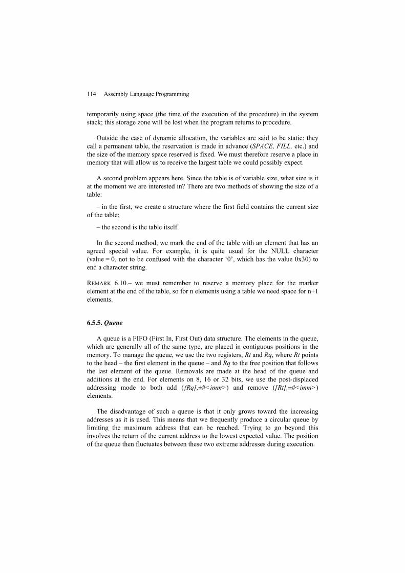
114 Assembly Language Programming
temporarily using space (the time of the execution of the procedure) in the systemstack; this storage zone will be lost when the program returns to procedure.
Outside the case of dynamic allocation, the variables are said to be static: theycall a permanent table, the reservation is made in advance (SPACE, FILL, etc.) andthe size of the memory space reserved is fixed. We must therefore reserve a place inmemory that will allow us to receive the largest table we could possibly expect.
A second problem appears here. Since the table is of variable size, what size is itat the moment we are interested in? There are two methods of showing the size of atable:
– in the first, we create a structure where the first field contains the current sizeof the table;
– the second is the table itself.
In the second method, we mark the end of the table with an element that has anagreed special value. For example, it is quite usual for the NULL character(value = 0, not to be confused with the character ‘0’, which has the value 0x30) toend a character string.
REMARK 6.10.– we must remember to reserve a memory place for the markerelement at the end of the table, so for n elements using a table we need space for n+1elements.
6.5.5. Queue
A queue is a FIFO (First In, First Out) data structure. The elements in the queue,which are generally all of the same type, are placed in contiguous positions in thememory. To manage the queue, we use the two registers, Rt and Rq, where Rt pointsto the head – the first element in the queue – and Rq to the free position that followsthe last element of the queue. Removals are made at the head of the queue andadditions at the end. For elements on 8, 16 or 32 bits, we use the post-displacedaddressing mode to both add ({Rq],±#<imm>) and remove ([Rt],±#<imm>)elements.
The disadvantage of such a queue is that it only grows toward the increasingaddresses as it is used. This means that we frequently produce a circular queue bylimiting the maximum address that can be reached. Trying to go beyond thisinvolves the return of the current address to the lowest expected value. The positionof the queue then fluctuates between these two extreme addresses during execution.
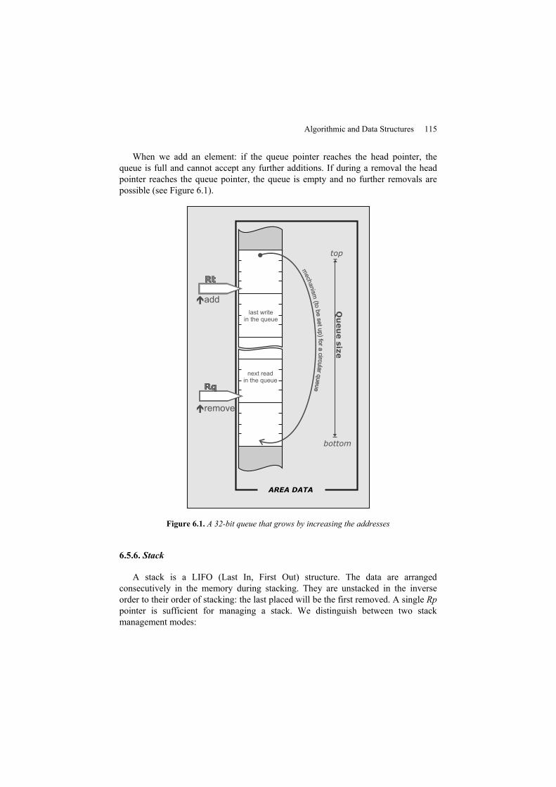
Algorithmic and Data Structures 115
When we add an element: if the queue pointer reaches the head pointer, thequeue is full and cannot accept any further additions. If during a removal the headpointer reaches the queue pointer, the queue is empty and no further removals arepossible (see Figure 6.1).
AREA DATA
top
bottom
remove
mech
anis
m(to
be
se
tup
)fo
ra
circ
ula
rq
ueue
mech
anis
m(to
be
se
tup
)fo
ra
circ
ula
rq
ueue
add
next readin the queue
last writein the queue
Figure 6.1. A 32-bit queue that grows by increasing the addresses
6.5.6. Stack
A stack is a LIFO (Last In, First Out) structure. The data are arrangedconsecutively in the memory during stacking. They are unstacked in the inverseorder to their order of stacking: the last placed will be the first removed. A single Rppointer is sufficient for managing a stack. We distinguish between two stackmanagement modes:
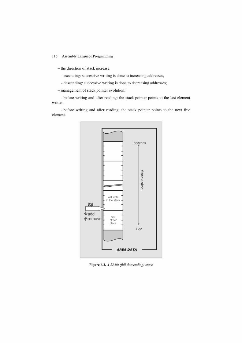
116 Assembly Language Programming
– the direction of stack increase:
- ascending: successive writing is done to increasing addresses,
- descending: successive writing is done to decreasing addresses;
– management of stack pointer evolution:
- before writing and after reading: the stack pointer points to the last elementwritten,
- before writing and after reading: the stack pointer points to the next freeelement.
AREA DATA
top
bottom
addremove
last writein the stack
first"free"place
Figure 6.2. A 32-bit (full descending) stack
Algorithmic and Data Structures 117
In the Cortex-M3 architecture, a LIFO stack mechanism exists in the hardware.It is managed by the stack pointer (SP, see section 2.2.2). This stack, called thesystem stack, is by default descending and with pre-decrementation in writing (alsoknown as a Full-Descending Stack), see Figure 6.2.
Be careful not to unalign a stack intended to receive words (or half-words,respectively). The address contained in the register must be doubly (respectivelysingly) even, i.e. ending with two (respectively, one) zero! This is the reason that itis not recommended that you construct a mixed stack where you stack bytes, half-words and words indiscriminately.
Queues and stacks of which the elements are not bytes nor half-words nor wordsare the most delicate to manage. It is necessary to calculate analog shifts similar tothose we have seen for tables. An often more advantageous technique consists ofadding a level of indirection by establishing stacks or queues consisting of theaddresses (references) of elements. The position and size of the elements are then ofno real importance.

Chapter 7
Internal Modularity
The concept of a procedure, a sequence of instructions able to be called as asubroutine, has been presented in section 3.3.5. In this chapter, we will look at howto use this elementary syntactic construction to write correct and easy to usesubroutines, by applying the principles of modular programming. We will see howto implement the passing of arguments to a subroutine and how to create localvariables.
7.1. Detailing the concept of procedure
7.1.1. Simple call
A procedure is a set of instructions designed to provide a particular service,usually ending with the instruction BX LR. The procedure, which may be called by aBL (Branch and Link) instruction, is placed in the calling procedure. This instructionsaves the return address (which we will denote @ret from now on) by using thelink register (LR) to store the value of the instruction pointer (also called theProgram Counter, PC) which contains the address of the instruction following thebranch, then jumps to the first instruction of the procedure being called. At the endof the procedure’s execution, the BX LR instruction restores the original PC value byloading the contents of the LR and execution resumes at the address following theBL. Example 7.1 illustrates this principle of a simple call to a procedure.
7.1.2. Nested calls
During a call, the return address is stored in a register. If the called procedureitself makes a call to a procedure, the call mechanism will automatically erase the
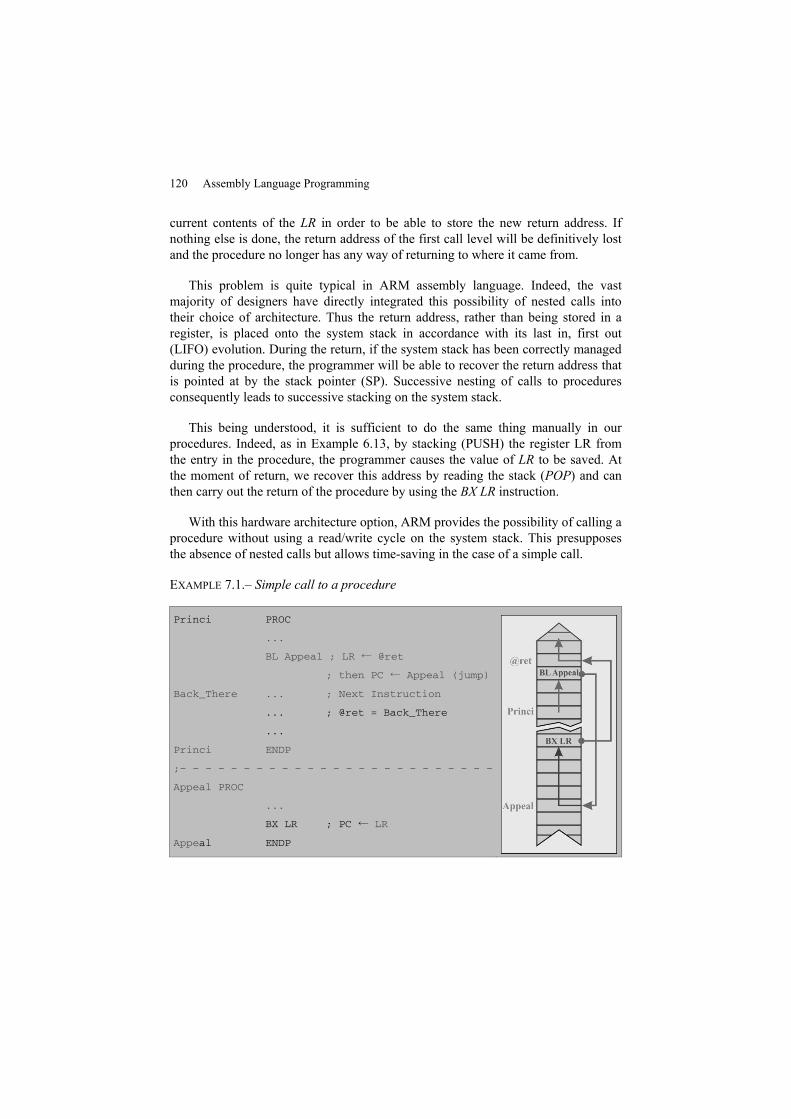
120 Assembly Language Programming
current contents of the LR in order to be able to store the new return address. Ifnothing else is done, the return address of the first call level will be definitively lostand the procedure no longer has any way of returning to where it came from.
This problem is quite typical in ARM assembly language. Indeed, the vastmajority of designers have directly integrated this possibility of nested calls intotheir choice of architecture. Thus the return address, rather than being stored in aregister, is placed onto the system stack in accordance with its last in, first out(LIFO) evolution. During the return, if the system stack has been correctly managedduring the procedure, the programmer will be able to recover the return address thatis pointed at by the stack pointer (SP). Successive nesting of calls to proceduresconsequently leads to successive stacking on the system stack.
This being understood, it is sufficient to do the same thing manually in ourprocedures. Indeed, as in Example 6.13, by stacking (PUSH) the register LR fromthe entry in the procedure, the programmer causes the value of LR to be saved. Atthe moment of return, we recover this address by reading the stack (POP) and canthen carry out the return of the procedure by using the BX LR instruction.
With this hardware architecture option, ARM provides the possibility of calling aprocedure without using a read/write cycle on the system stack. This presupposesthe absence of nested calls but allows time-saving in the case of a simple call.
EXAMPLE 7.1.– Simple call to a procedure
Princi PROC
...
BL Appeal ; LR ← @ret
; then PC ← Appeal (jump)
Back_There ... ; Next Instruction
... ; @ret = Back_There
...
Princi ENDP
;– – – – – – – – – – – – – – – – – – – – – – – – –
Appeal PROC
...
BX LR ; PC ← LR
Appeal ENDP
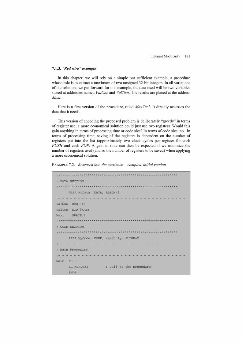
Internal Modularity 121
7.1.3. “Red wire” example
In this chapter, we will rely on a simple but sufficient example: a procedurewhose role is to extract a maximum of two unsigned 32-bit integers. In all variationsof the solutions we put forward for this example, the data used will be two variablesstored at addresses named ValOne and ValTwo. The results are placed at the addressMaxi.
Here is a first version of the procedure, titled MaxVer1. It directly accesses thedata that it needs.
This version of encoding the proposed problem is deliberately “greedy” in termsof register use; a more economical solution could just use two registers. Would thisgain anything in terms of processing time or code size? In terms of code size, no. Interms of processing time, saving of the registers is dependent on the number ofregisters put into the list (approximately two clock cycles per register for eachPUSH and each POP. A gain in time can then be expected if we minimize thenumber of registers used (and so the number of registers to be saved) when applyinga more economical solution.
EXAMPLE 7.2.– Research into the maximum – complete initial version
;*************************************************************
; DATA SECTION
;*************************************************************
AREA MyData, DATA, ALIGN=2
;– – – – – – – – – – – – – – – – – – – – – – – – – – – – – – – – –
ValOne DCD 345
ValTwo DCD 0xABF
Maxi SPACE 4
;*************************************************************
; CODE SECTION
;*************************************************************
AREA MyCode, CODE, readonly, ALIGN=2
;– – – – – – – – – – – – – – – – – – – – – – – – – – – – – – – – –
; Main Procedure
;– – – – – – – – – – – – – – – – – – – – – – – – – – – – – – – – –
main PROC
BL MaxVer1 ; Call to the procedure
ENDP
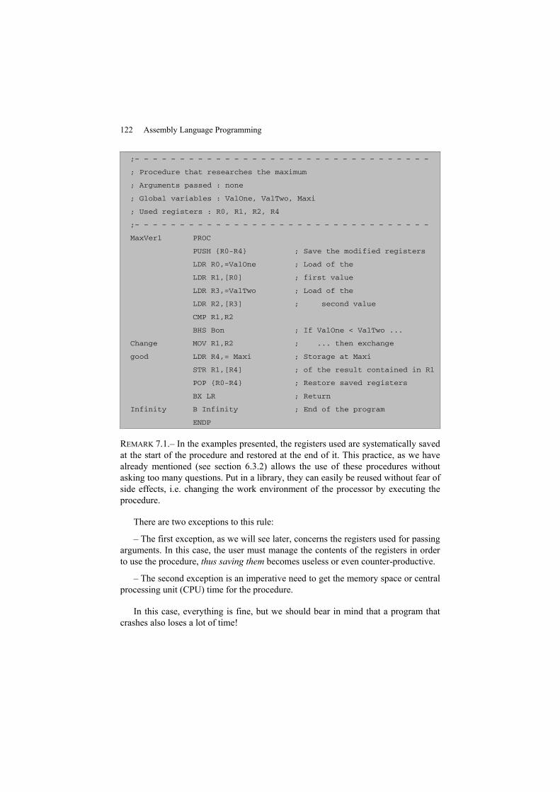
122 Assembly Language Programming
;– – – – – – – – – – – – – – – – – – – – – – – – – – – – – – – – –
; Procedure that researches the maximum
; Arguments passed : none
; Global variables : ValOne, ValTwo, Maxi
; Used registers : R0, R1, R2, R4
;– – – – – – – – – – – – – – – – – – – – – – – – – – – – – – – – –
MaxVer1 PROC
PUSH {R0-R4} ; Save the modified registers
LDR R0,=ValOne ; Load of the
LDR R1,[R0] ; first value
LDR R3,=ValTwo ; Load of the
LDR R2,[R3] ; second value
CMP R1,R2
BHS Bon ; If ValOne < ValTwo ...
Change MOV R1,R2 ; ... then exchange
good LDR R4,= Maxi ; Storage at Maxi
STR R1,[R4] ; of the result contained in R1
POP {R0-R4} ; Restore saved registers
BX LR ; Return
Infinity B Infinity ; End of the program
ENDP
REMARK 7.1.– In the examples presented, the registers used are systematically savedat the start of the procedure and restored at the end of it. This practice, as we havealready mentioned (see section 6.3.2) allows the use of these procedures withoutasking too many questions. Put in a library, they can easily be reused without fear ofside effects, i.e. changing the work environment of the processor by executing theprocedure.
There are two exceptions to this rule:
– The first exception, as we will see later, concerns the registers used for passingarguments. In this case, the user must manage the contents of the registers in orderto use the procedure, thus saving them becomes useless or even counter-productive.
– The second exception is an imperative need to get the memory space or centralprocessing unit (CPU) time for the procedure.
In this case, everything is fine, but we should bear in mind that a program thatcrashes also loses a lot of time!
Internal Modularity 123
7.2. Procedure arguments
7.2.1. Usefulness of arguments
From the point of view of the calling program, the MaxVer1 procedure changesthe value of the result at the Maxi address by using the values recorded in ValOneand ValTwo. Written like this, such a procedure is hardly satisfying because it isnecessary to give it data with specific names, which makes it impossible to reuse theprocedure in another program, unless we always use the same names for the data.
Also, in modular programming, it is recommended that we avoid directly usingglobal variables. This is made possible by the use of explicit call arguments. Thesubroutine then becomes easily reusable if it follows the conventional rules forpassing arguments.
7.2.2. Arguments by value and by reference
Each argument can be passed by value or reference. If it is passed by value, acopy of the data is provided to the called by the calling procedure, so that itspotential modification by the latter does not affect the original: the modificationremains local to the subroutine called. When an argument is passed by reference, weprovide the address to the subroutine that, by indirection, could possibly change thevalue of the data at that address.
No assembly language has instructions to call a subroutine incorporating theconcept of argument, and the BL instruction for Cortex-M3 is no exception; ittherefore raises the question of by which mechanisms it is possible to provide aprocedure with the values or the relative addresses of the arguments. Essentially,there are two techniques, but both can be reduced to the same basic idea: argumentsare positioned according to an agreed order in a predetermined region of thememory.
7.2.3. Passing arguments by general registers
General registers provide an initial easy, quick and effective method of passingarguments. The values of arguments or their addresses (references) are placed in theagreed registers and the procedure can be used immediately.
7.2.3.1. Passing arguments by value
In our example, we have three arguments to consider: the two pieces of data atentry, and the result at exit. Here is a first modification of the example (MaxVer2)
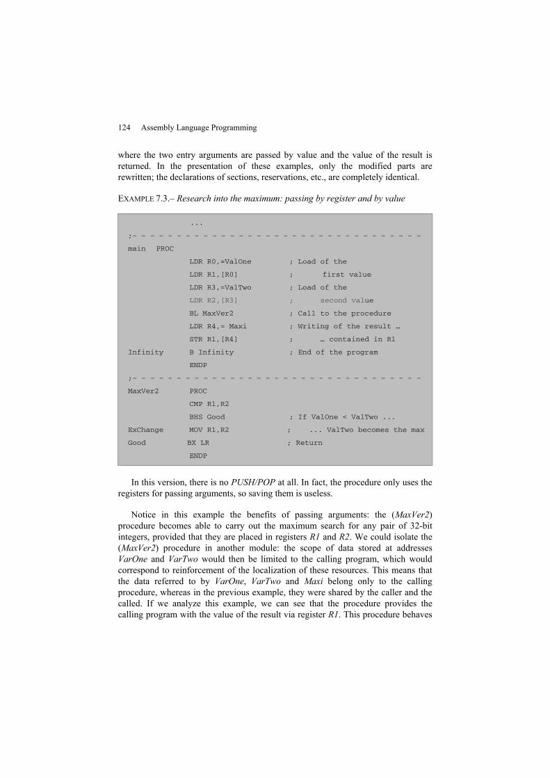
124 Assembly Language Programming
where the two entry arguments are passed by value and the value of the result isreturned. In the presentation of these examples, only the modified parts arerewritten; the declarations of sections, reservations, etc., are completely identical.
EXAMPLE 7.3.– Research into the maximum: passing by register and by value
...
;– – – – – – – – – – – – – – – – – – – – – – – – – – – – – – – – –
main PROC
LDR R0,=ValOne ; Load of the
LDR R1,[R0] ; first value
LDR R3,=ValTwo ; Load of the
LDR R2,[R3] ; second value
BL MaxVer2 ; Call to the procedure
LDR R4,= Maxi ; Writing of the result …
STR R1,[R4] ; … contained in R1
Infinity B Infinity ; End of the program
ENDP
;– – – – – – – – – – – – – – – – – – – – – – – – – – – – – – – – –
MaxVer2 PROC
CMP R1,R2
BHS Good ; If ValOne < ValTwo ...
ExChange MOV R1,R2 ; ... ValTwo becomes the max
Good BX LR ; Return
ENDP
In this version, there is no PUSH/POP at all. In fact, the procedure only uses theregisters for passing arguments, so saving them is useless.
Notice in this example the benefits of passing arguments: the (MaxVer2)procedure becomes able to carry out the maximum search for any pair of 32-bitintegers, provided that they are placed in registers R1 and R2. We could isolate the(MaxVer2) procedure in another module: the scope of data stored at addressesVarOne and VarTwo would then be limited to the calling program, which wouldcorrespond to reinforcement of the localization of these resources. This means thatthe data referred to by VarOne, VarTwo and Maxi belong only to the callingprocedure, whereas in the previous example, they were shared by the caller and thecalled. If we analyze this example, we can see that the procedure provides thecalling program with the value of the result via register R1. This procedure behaves
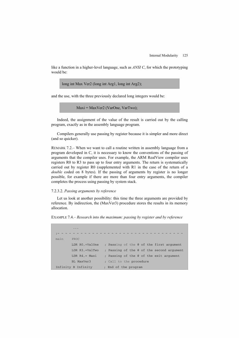
Internal Modularity 125
like a function in a higher-level language, such as ANSI C, for which the prototypingwould be:
long int Max Ver2 (long int Arg1, long int Arg2);
and the use, with the three previously declared long integers would be:
Maxi = MaxVer2 (VarOne, VarTwo);
Indeed, the assignment of the value of the result is carried out by the callingprogram, exactly as in the assembly language program.
Compilers generally use passing by register because it is simpler and more direct(and so quicker).
REMARK 7.2.– When we want to call a routine written in assembly language from aprogram developed in C, it is necessary to know the conventions of the passing ofarguments that the compiler uses. For example, the ARM RealView compiler usesregisters R0 to R3 to pass up to four entry arguments. The return is systematicallycarried out by register R0 (supplemented with R1 in the case of the return of adouble coded on 8 bytes). If the passing of arguments by register is no longerpossible, for example if there are more than four entry arguments, the compilercompletes the process using passing by system stack.
7.2.3.2. Passing arguments by reference
Let us look at another possibility: this time the three arguments are provided byreference. By indirection, the (MaxVer3) procedure stores the results in its memoryallocation.
EXAMPLE 7.4.– Research into the maximum: passing by register and by reference
...
;– – – – – – – – – – – – – – – – – – – – – – – – – – – – – – – – –
main PROC
LDR R0,=ValOne ; Passing of the @ of the first argument
LDR R3,=ValTwo ; Passing of the @ of the second argument
LDR R4,= Maxi ; Passing of the @ of the exit argument
BL MaxVer3 ; Call to the procedure
Infinity B Infinity ; End of the program
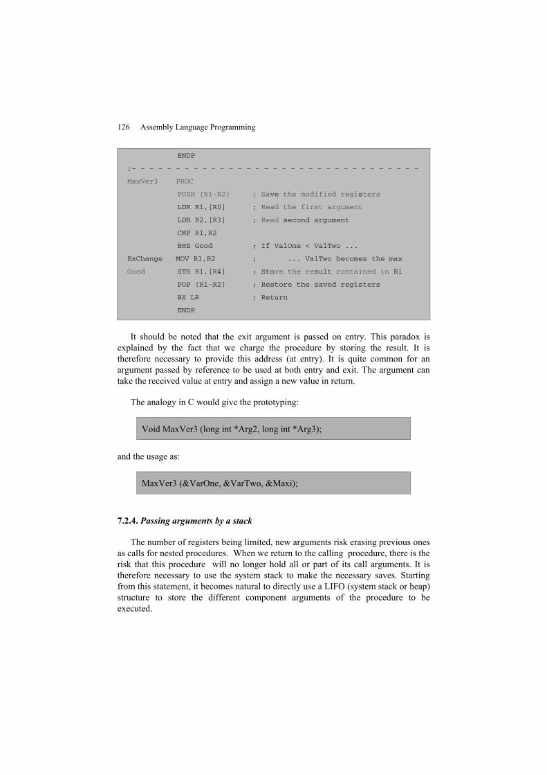
126 Assembly Language Programming
ENDP
;– – – – – – – – – – – – – – – – – – – – – – – – – – – – – – – – –
MaxVer3 PROC
PUSH {R1-R2} ; Save the modified registers
LDR R1,[R0] ; Read the first argument
LDR R2,[R3] ; Read second argument
CMP R1,R2
BHS Good ; If ValOne < ValTwo ...
ExChange MOV R1,R2 ; ... ValTwo becomes the max
Good STR R1,[R4] ; Store the result contained in R1
POP {R1-R2} ; Restore the saved registers
BX LR ; Return
ENDP
It should be noted that the exit argument is passed on entry. This paradox isexplained by the fact that we charge the procedure by storing the result. It istherefore necessary to provide this address (at entry). It is quite common for anargument passed by reference to be used at both entry and exit. The argument cantake the received value at entry and assign a new value in return.
The analogy in C would give the prototyping:
Void MaxVer3 (long int *Arg2, long int *Arg3);
and the usage as:
MaxVer3 (&VarOne, &VarTwo, &Maxi);
7.2.4. Passing arguments by a stack
The number of registers being limited, new arguments risk erasing previous onesas calls for nested procedures. When we return to the calling procedure, there is therisk that this procedure will no longer hold all or part of its call arguments. It istherefore necessary to use the system stack to make the necessary saves. Startingfrom this statement, it becomes natural to directly use a LIFO (system stack or heap)structure to store the different component arguments of the procedure to beexecuted.
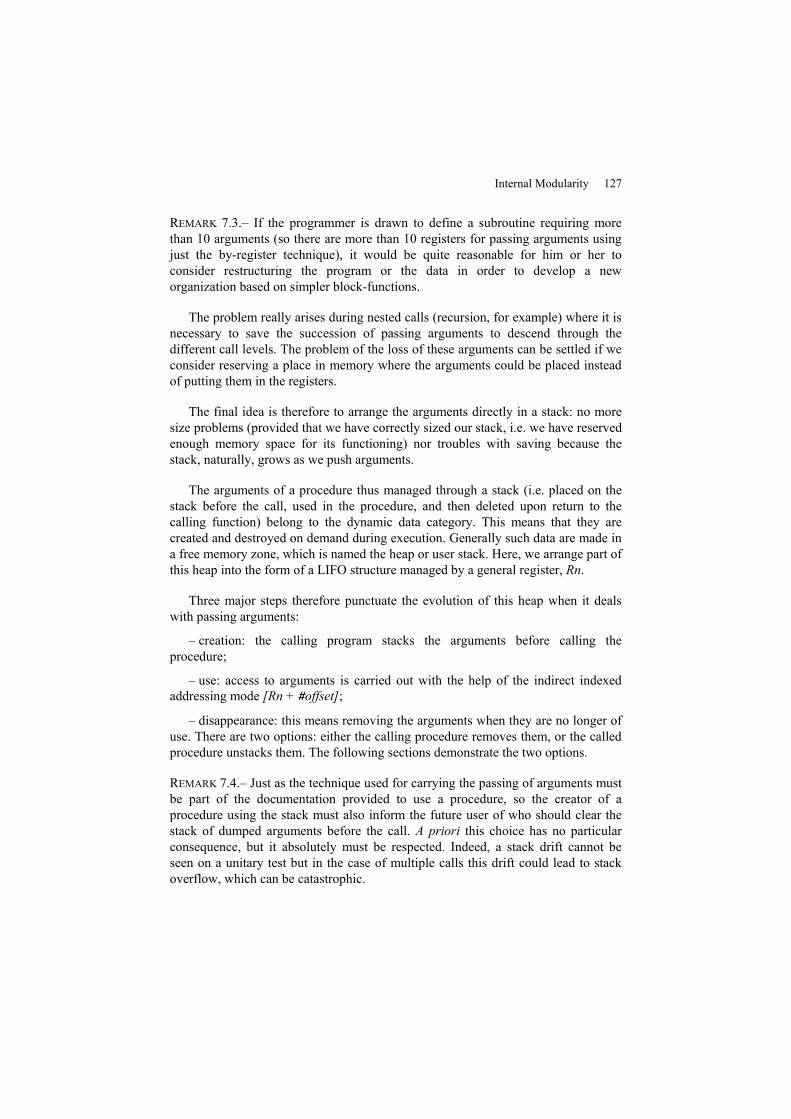
Internal Modularity 127
REMARK 7.3.– If the programmer is drawn to define a subroutine requiring morethan 10 arguments (so there are more than 10 registers for passing arguments usingjust the by-register technique), it would be quite reasonable for him or her toconsider restructuring the program or the data in order to develop a neworganization based on simpler block-functions.
The problem really arises during nested calls (recursion, for example) where it isnecessary to save the succession of passing arguments to descend through thedifferent call levels. The problem of the loss of these arguments can be settled if weconsider reserving a place in memory where the arguments could be placed insteadof putting them in the registers.
The final idea is therefore to arrange the arguments directly in a stack: no moresize problems (provided that we have correctly sized our stack, i.e. we have reservedenough memory space for its functioning) nor troubles with saving because thestack, naturally, grows as we push arguments.
The arguments of a procedure thus managed through a stack (i.e. placed on thestack before the call, used in the procedure, and then deleted upon return to thecalling function) belong to the dynamic data category. This means that they arecreated and destroyed on demand during execution. Generally such data are made ina free memory zone, which is named the heap or user stack. Here, we arrange part ofthis heap into the form of a LIFO structure managed by a general register, Rn.
Three major steps therefore punctuate the evolution of this heap when it dealswith passing arguments:
– creation: the calling program stacks the arguments before calling theprocedure;
– use: access to arguments is carried out with the help of the indirect indexedaddressing mode [Rn + #offset];
– disappearance: this means removing the arguments when they are no longer ofuse. There are two options: either the calling procedure removes them, or the calledprocedure unstacks them. The following sections demonstrate the two options.
REMARK 7.4.– Just as the technique used for carrying the passing of arguments mustbe part of the documentation provided to use a procedure, so the creator of aprocedure using the stack must also inform the future user of who should clear thestack of dumped arguments before the call. A priori this choice has no particularconsequence, but it absolutely must be respected. Indeed, a stack drift cannot beseen on a unitary test but in the case of multiple calls this drift could lead to stackoverflow, which can be catastrophic.
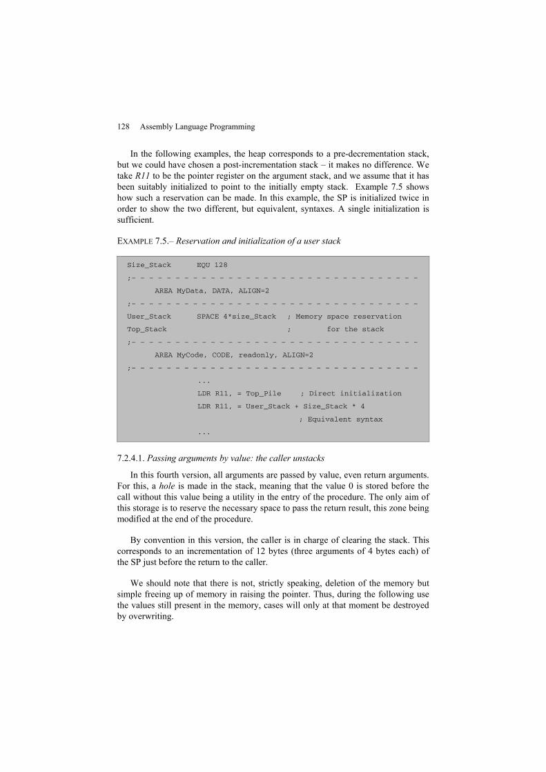
128 Assembly Language Programming
In the following examples, the heap corresponds to a pre-decrementation stack,but we could have chosen a post-incrementation stack – it makes no difference. Wetake R11 to be the pointer register on the argument stack, and we assume that it hasbeen suitably initialized to point to the initially empty stack. Example 7.5 showshow such a reservation can be made. In this example, the SP is initialized twice inorder to show the two different, but equivalent, syntaxes. A single initialization issufficient.
EXAMPLE 7.5.– Reservation and initialization of a user stack
Size_Stack EQU 128
;– – – – – – – – – – – – – – – – – – – – – – – – – – – – – – – – –
AREA MyData, DATA, ALIGN=2
;– – – – – – – – – – – – – – – – – – – – – – – – – – – – – – – – –
User_Stack SPACE 4*size_Stack ; Memory space reservation
Top_Stack ; for the stack
;– – – – – – – – – – – – – – – – – – – – – – – – – – – – – – – – –
AREA MyCode, CODE, readonly, ALIGN=2
;– – – – – – – – – – – – – – – – – – – – – – – – – – – – – – – – –
...
LDR R11, = Top_Pile ; Direct initialization
LDR R11, = User_Stack + Size_Stack * 4
; Equivalent syntax
...
7.2.4.1. Passing arguments by value: the caller unstacks
In this fourth version, all arguments are passed by value, even return arguments.For this, a hole is made in the stack, meaning that the value 0 is stored before thecall without this value being a utility in the entry of the procedure. The only aim ofthis storage is to reserve the necessary space to pass the return result, this zone beingmodified at the end of the procedure.
By convention in this version, the caller is in charge of clearing the stack. Thiscorresponds to an incrementation of 12 bytes (three arguments of 4 bytes each) ofthe SP just before the return to the caller.
We should note that there is not, strictly speaking, deletion of the memory butsimple freeing up of memory in raising the pointer. Thus, during the following usethe values still present in the memory, cases will only at that moment be destroyedby overwriting.
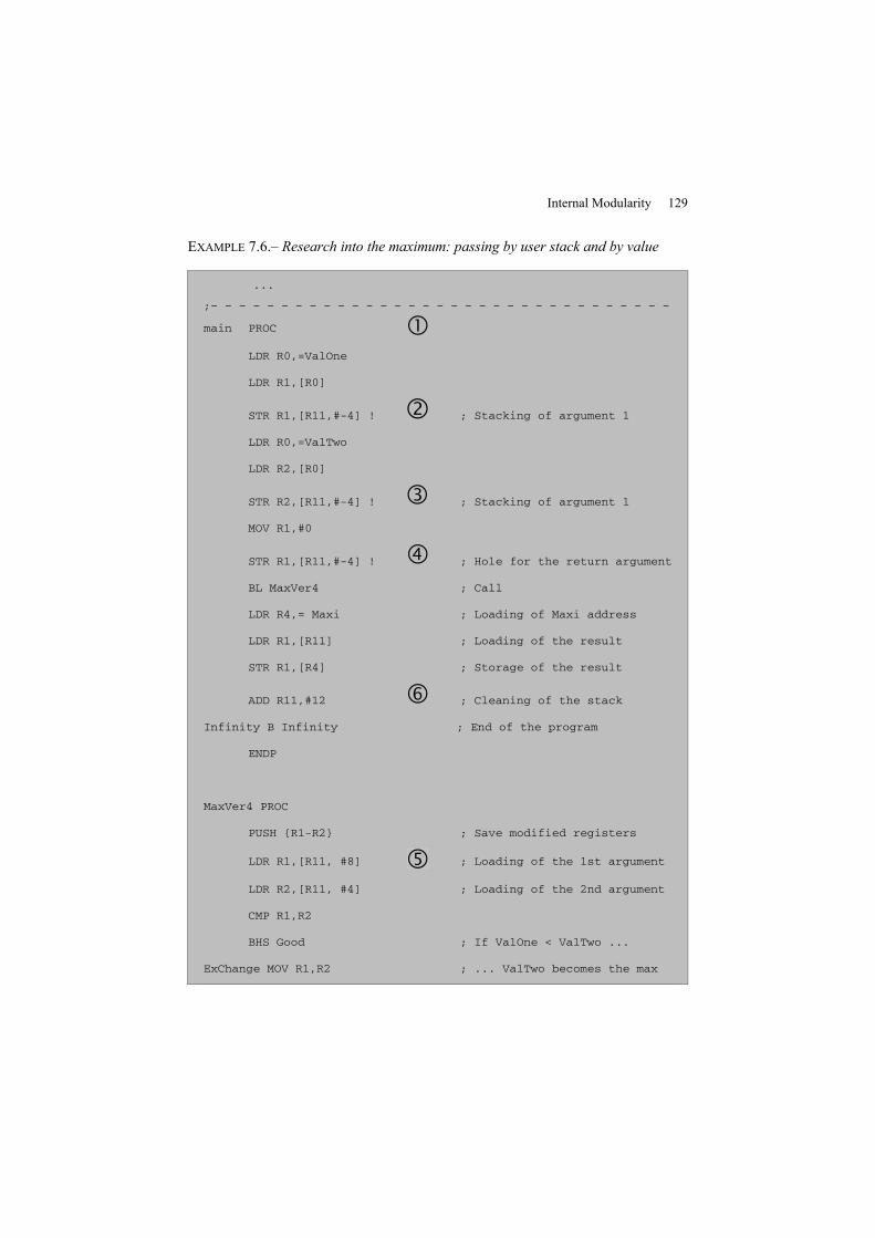
Internal Modularity 129
EXAMPLE 7.6.– Research into the maximum: passing by user stack and by value
...
;– – – – – – – – – – – – – – – – – – – – – – – – – – – – – – – – –
main PROC
LDR R0,=ValOne
LDR R1,[R0]
STR R1,[R11,#-4] ! ; Stacking of argument 1
LDR R0,=ValTwo
LDR R2,[R0]
STR R2,[R11,#-4] ! ; Stacking of argument 1
MOV R1,#0
STR R1,[R11,#-4] ! ; Hole for the return argument
BL MaxVer4 ; Call
LDR R4,= Maxi ; Loading of Maxi address
LDR R1,[R11] ; Loading of the result
STR R1,[R4] ; Storage of the result
ADD R11,#12 ; Cleaning of the stack
Infinity B Infinity ; End of the program
ENDP
MaxVer4 PROC
PUSH {R1-R2} ; Save modified registers
LDR R1,[R11, #8] ; Loading of the 1st argument
LDR R2,[R11, #4] ; Loading of the 2nd argument
CMP R1,R2
BHS Good ; If ValOne < ValTwo ...
ExChange MOV R1,R2 ; ... ValTwo becomes the max
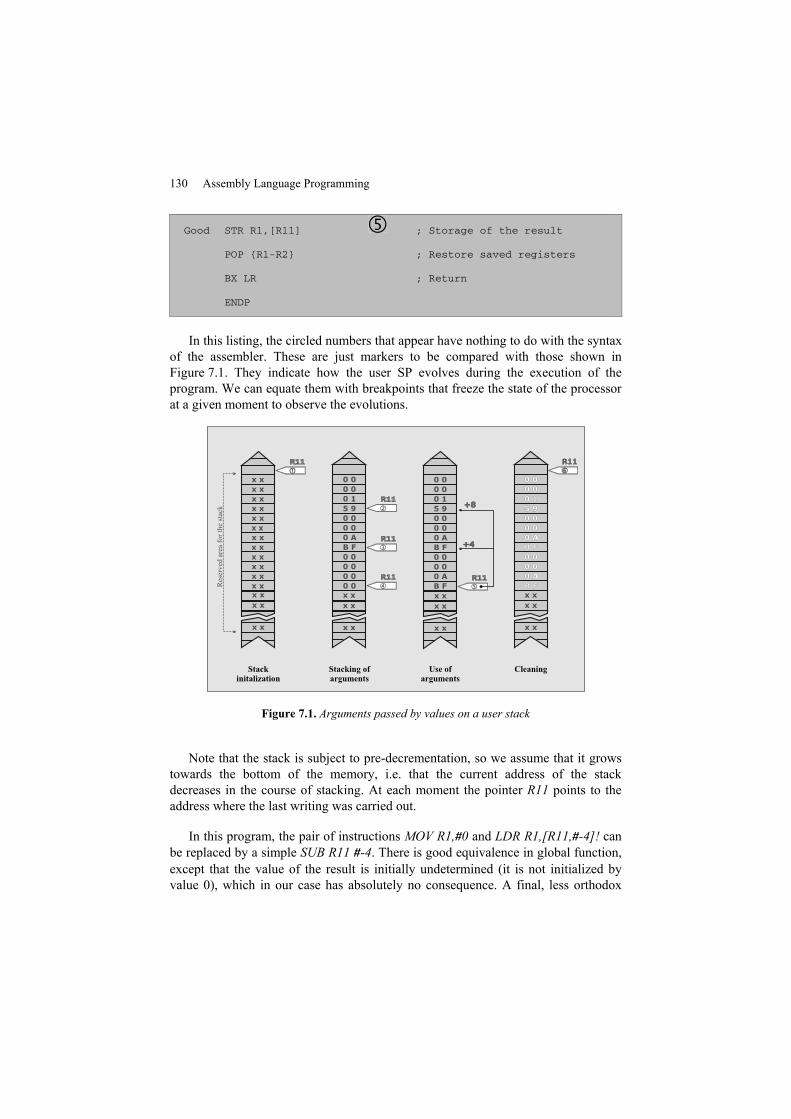
130 Assembly Language Programming
Good STR R1,[R11] ; Storage of the result
POP {R1-R2} ; Restore saved registers
BX LR ; Return
ENDP
In this listing, the circled numbers that appear have nothing to do with the syntaxof the assembler. These are just markers to be compared with those shown inFigure 7.1. They indicate how the user SP evolves during the execution of theprogram. We can equate them with breakpoints that freeze the state of the processorat a given moment to observe the evolutions.
Reserv
ed
are
afo
rth
esta
ck
0 00 0
0 00 0
0 10 1
5 95 9
0 00 0
0 00 0
0 A0 A
B FB F
0 00 0
0 00 0
0 A0 A
B FB F
Stackinitalization
Stacking ofarguments
Use ofarguments
Cleaning
x x
x x
x x
0 0
0 0
0 1
5 9
0 0
0 0
0 A
B F
0 0
0 0
0 A
B F
x x
x x
x x
0 0x x
0 0x x
0 1x x
5 9x x
0 0x x
0 0x x
0 Ax x
B Fx x
0 0x x
0 0x x
0 0x x
0 0x xx x
x x
x x
x x
x x
x x
+4+4
+8+8
Figure 7.1. Arguments passed by values on a user stack
Note that the stack is subject to pre-decrementation, so we assume that it growstowards the bottom of the memory, i.e. that the current address of the stackdecreases in the course of stacking. At each moment the pointer R11 points to theaddress where the last writing was carried out.
In this program, the pair of instructions MOV R1,#0 and LDR R1,[R11,#-4]! canbe replaced by a simple SUB R11 #-4. There is good equivalence in global function,except that the value of the result is initially undetermined (it is not initialized byvalue 0), which in our case has absolutely no consequence. A final, less orthodox
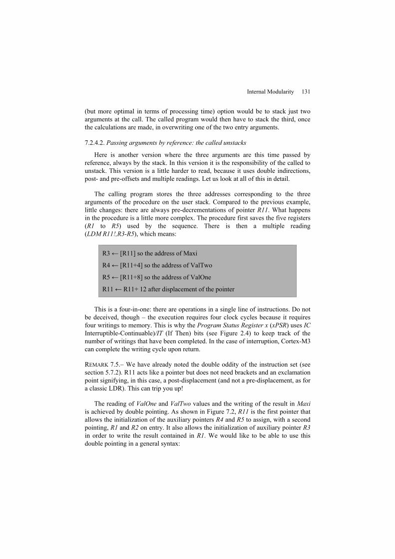
Internal Modularity 131
(but more optimal in terms of processing time) option would be to stack just twoarguments at the call. The called program would then have to stack the third, oncethe calculations are made, in overwriting one of the two entry arguments.
7.2.4.2. Passing arguments by reference: the called unstacks
Here is another version where the three arguments are this time passed byreference, always by the stack. In this version it is the responsibility of the called tounstack. This version is a little harder to read, because it uses double indirections,post- and pre-offsets and multiple readings. Let us look at all of this in detail.
The calling program stores the three addresses corresponding to the threearguments of the procedure on the user stack. Compared to the previous example,little changes: there are always pre-decrementations of pointer R11. What happensin the procedure is a little more complex. The procedure first saves the five registers(R1 to R5) used by the sequence. There is then a multiple reading(LDM R11!,R3-R5), which means:
R3← [R11] so the address of Maxi
R4← [R11+4] so the address of ValTwo
R5← [R11+8] so the address of ValOne
R11← R11+ 12 after displacement of the pointer
This is a four-in-one: there are operations in a single line of instructions. Do notbe deceived, though – the execution requires four clock cycles because it requiresfour writings to memory. This is why the Program Status Register x (xPSR) uses ICInterruptible-Continuable)/IT (If Then) bits (see Figure 2.4) to keep track of thenumber of writings that have been completed. In the case of interruption, Cortex-M3can complete the writing cycle upon return.
REMARK 7.5.– We have already noted the double oddity of the instruction set (seesection 5.7.2). R11 acts like a pointer but does not need brackets and an exclamationpoint signifying, in this case, a post-displacement (and not a pre-displacement, as fora classic LDR). This can trip you up!
The reading of ValOne and ValTwo values and the writing of the result in Maxiis achieved by double pointing. As shown in Figure 7.2, R11 is the first pointer thatallows the initialization of the auxiliary pointers R4 and R5 to assign, with a secondpointing, R1 and R2 on entry. It also allows the initialization of auxiliary pointer R3in order to write the result contained in R1. We would like to be able to use thisdouble pointing in a general syntax:
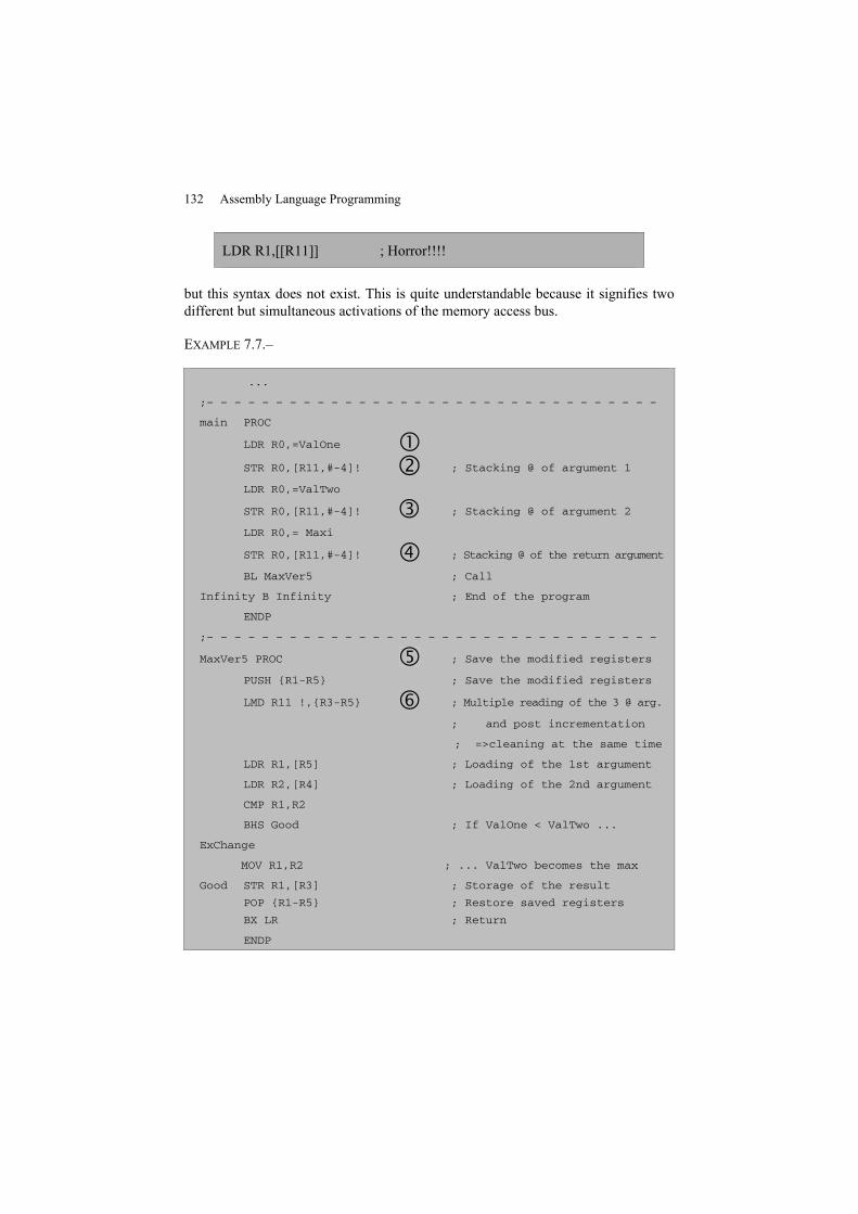
132 Assembly Language Programming
LDR R1,[[R11]] ; Horror!!!!
but this syntax does not exist. This is quite understandable because it signifies twodifferent but simultaneous activations of the memory access bus.
EXAMPLE 7.7.–
...
;– – – – – – – – – – – – – – – – – – – – – – – – – – – – – – – – –
main PROC
LDR R0,=ValOne
STR R0,[R11,#-4]! ; Stacking @ of argument 1
LDR R0,=ValTwo
STR R0,[R11,#-4]! ; Stacking @ of argument 2
LDR R0,= Maxi
STR R0,[R11,#-4]! ; Stacking @ of the return argument
BL MaxVer5 ; Call
Infinity B Infinity ; End of the program
ENDP
;– – – – – – – – – – – – – – – – – – – – – – – – – – – – – – – – –
MaxVer5 PROC ; Save the modified registers
PUSH {R1-R5} ; Save the modified registers
LMD R11 !,{R3-R5} ; Multiple reading of the 3 @ arg.
; and post incrementation
; =>cleaning at the same time
LDR R1,[R5] ; Loading of the 1st argument
LDR R2,[R4] ; Loading of the 2nd argument
CMP R1,R2
BHS Good ; If ValOne < ValTwo ...
ExChange
MOV R1,R2 ; ... ValTwo becomes the max
Good STR R1,[R3] ; Storage of the result
POP {R1-R5} ; Restore saved registers
BX LR ; Return
ENDP
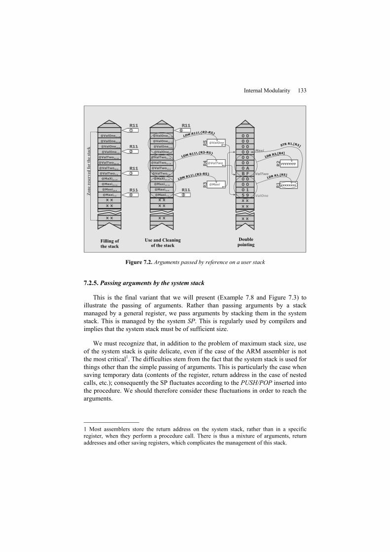
Internal Modularity 133Z
on
ere
serv
edfo
rth
est
ack
Filling ofthe stack
Use and Cleaningof the stack
@ValOne31-24
@ValOne23-16
@ValOne15-8
@ValOne7-0
x x
x x
x x
@ValTwo31-24
@ValTwo23-16
@ValTwo15-8
@ValTwo7-0
@MaXi31-24
@Maxi23-16
@Maxi15-8
@Maxi7-0
@ValOne31-24
@ValOne23-16
@ValOne15-8
@ValOne7-0
x x
x x
x x
@ValTwo31-24
@ValTwo23-16
@ValTwo15-8
@ValTwo7-0
@MaXi31-24
@Maxi23-16
@Maxi15-8
@Maxi7-0
R5
R5 @ValOne
R1
R1 xxxxxxxxR3
R3 @Maxi
R4
R4 @ValTwo
LDM R11!,{R3-R5}
LDM R11!,{R3-R5}
LDM R11!,{R3-R5}
LDR R1,[R5]
R2
R2 yyyyyyyy
LDR R2,[R4]
LDR R2,[R4]
STR R1,[R3]
0 0
0 0
0 0
0 0
0 0
0 0
0 A
B F
0 0
0 0
0 1
5 9
x x
x x
x x
Doublepointing
ValOne
ValTwo
Maxi
Figure 7.2. Arguments passed by reference on a user stack
7.2.5. Passing arguments by the system stack
This is the final variant that we will present (Example 7.8 and Figure 7.3) toillustrate the passing of arguments. Rather than passing arguments by a stackmanaged by a general register, we pass arguments by stacking them in the systemstack. This is managed by the system SP. This is regularly used by compilers andimplies that the system stack must be of sufficient size.
We must recognize that, in addition to the problem of maximum stack size, useof the system stack is quite delicate, even if the case of the ARM assembler is notthe most critical1. The difficulties stem from the fact that the system stack is used forthings other than the simple passing of arguments. This is particularly the case whensaving temporary data (contents of the register, return address in the case of nestedcalls, etc.); consequently the SP fluctuates according to the PUSH/POP inserted intothe procedure. We should therefore consider these fluctuations in order to reach thearguments.
1 Most assemblers store the return address on the system stack, rather than in a specificregister, when they perform a procedure call. There is thus a mixture of arguments, returnaddresses and other saving registers, which complicates the management of this stack.
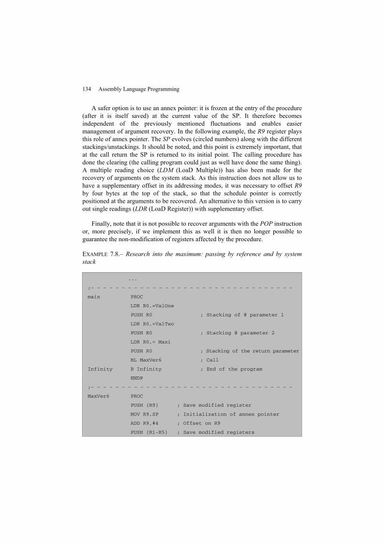
134 Assembly Language Programming
A safer option is to use an annex pointer: it is frozen at the entry of the procedure(after it is itself saved) at the current value of the SP. It therefore becomesindependent of the previously mentioned fluctuations and enables easiermanagement of argument recovery. In the following example, the R9 register playsthis role of annex pointer. The SP evolves (circled numbers) along with the differentstackings/unstackings. It should be noted, and this point is extremely important, thatat the call return the SP is returned to its initial point. The calling procedure hasdone the clearing (the calling program could just as well have done the same thing).A multiple reading choice (LDM (LoaD Multiple)) has also been made for therecovery of arguments on the system stack. As this instruction does not allow us tohave a supplementary offset in its addressing modes, it was necessary to offset R9by four bytes at the top of the stack, so that the schedule pointer is correctlypositioned at the arguments to be recovered. An alternative to this version is to carryout single readings (LDR (LoaD Register)) with supplementary offset.
Finally, note that it is not possible to recover arguments with the POP instructionor, more precisely, if we implement this as well it is then no longer possible toguarantee the non-modification of registers affected by the procedure.
EXAMPLE 7.8.– Research into the maximum: passing by reference and by systemstack
...
;– – – – – – – – – – – – – – – – – – – – – – – – – – – – – – – – –
main PROC
LDR R0,=ValOne
PUSH R0 ; Stacking of @ parameter 1
LDR R0,=ValTwo
PUSH R0 ; Stacking @ parameter 2
LDR R0,= Maxi
PUSH R0 ; Stacking of the return parameter
BL MaxVer6 ; Call
Infinity B Infinity ; End of the program
ENDP
;– – – – – – – – – – – – – – – – – – – – – – – – – – – – – – – – –
MaxVer6 PROC
PUSH {R9} ; Save modified register
MOV R9,SP ; Initialization of annex pointer
ADD R9,#4 ; Offset on R9
PUSH {R1-R5} ; Save modified registers
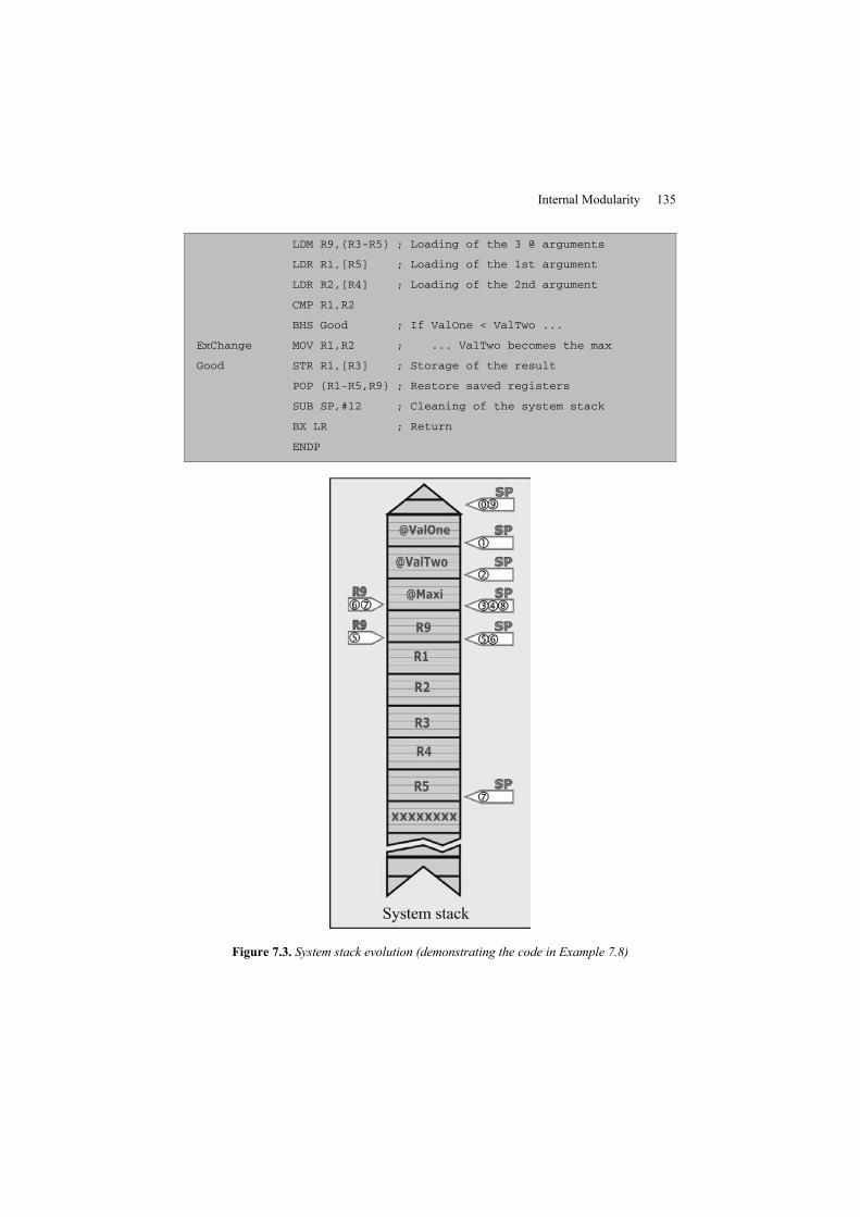
Internal Modularity 135
LDM R9,{R3-R5} ; Loading of the 3 @ arguments
LDR R1,[R5] ; Loading of the 1st argument
LDR R2,[R4] ; Loading of the 2nd argument
CMP R1,R2
BHS Good ; If ValOne < ValTwo ...
ExChange MOV R1,R2 ; ... ValTwo becomes the max
Good STR R1,[R3] ; Storage of the result
POP {R1-R5,R9} ; Restore saved registers
SUB SP,#12 ; Cleaning of the system stack
BX LR ; Return
ENDP
Figure 7.3. System stack evolution (demonstrating the code in Example 7.8)
136 Assembly Language Programming
7.2.6. On the art of mixing
All of the versions of passing arguments that have been presented in the previoussections can mix at will. This is both the strength and the flexibility of programmingin assembly language, but it is also the difficulty. We can in fact, and for example,pass a first argument by value and by register, a second by reference and by systemstack and recover the results of the procedure on a user stack. It is easy tounderstand that such a mixture risks causing terrible problems. Thus, unless you areobliged (by motivations that can appear obscure) to do so, it is best to avoid mixing.
7.3. Local data
To carry out its work, a subroutine may have to use its own data. These are thelocal data of the subroutine. The rule of localization invites us to place these data sothat they are only visible and usable by the proprietary subroutine. The simplest wayof doing this in assembly language is to use the general registers to contain the localvariables. It works perfectly in simple cases, especially if the local data are not toonumerous. Unfortunately, the number of registers is limited. What is more, thismethod is not usable in the case of calls to nested subroutines or for a recursivefunction without needing several saves. We could consider planning the creation ofthese local data in a specific data section, but this leads to a “waste” of memorybecause it is only used during the execution of the procedure. A more satisfactorysolution would be to superimpose all of these sections by specifying them as beingCOMMON, that is specifying them as attributes in the declaration of the section:AREA Mydata DATA align=2, COMMON, so that they share the same portion ofmemory. We can, however, apply the same criticism to this method ofsuperimposition as for the case of arguments arranged in a fixed space: the launch ofa subroutine can lead to a partial or total loss of local data from the calling program.We therefore prefer to create the data in a dynamic manner at the beginning of theexecution of the procedure. Here are two options, both using the heap:
– in addition to the stack for the arguments, we use a second stack for the localvariables;
– during execution we place them on the same stack as the arguments.
REMARK 7.6.– Local variables dynamically created on a stack can equally be createdon a user stack (a heap) or on the system stack. As in the case of passing arguments,the use of the system stack is more delicate, and therefore dangerous. As such, ifthere are no imperatives linked to memory use, it is always preferable and safer touse the user stack itself.
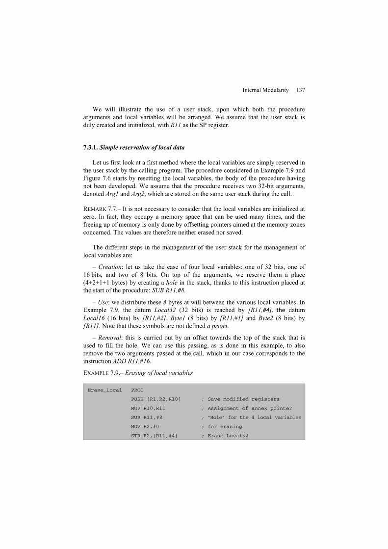
Internal Modularity 137
We will illustrate the use of a user stack, upon which both the procedurearguments and local variables will be arranged. We assume that the user stack isduly created and initialized, with R11 as the SP register.
7.3.1. Simple reservation of local data
Let us first look at a first method where the local variables are simply reserved inthe user stack by the calling program. The procedure considered in Example 7.9 andFigure 7.6 starts by resetting the local variables, the body of the procedure havingnot been developed. We assume that the procedure receives two 32-bit arguments,denoted Arg1 and Arg2, which are stored on the same user stack during the call.
REMARK 7.7.– It is not necessary to consider that the local variables are initialized atzero. In fact, they occupy a memory space that can be used many times, and thefreeing up of memory is only done by offsetting pointers aimed at the memory zonesconcerned. The values are therefore neither erased nor saved.
The different steps in the management of the user stack for the management oflocal variables are:
– Creation: let us take the case of four local variables: one of 32 bits, one of16 bits, and two of 8 bits. On top of the arguments, we reserve them a place(4+2+1+1 bytes) by creating a hole in the stack, thanks to this instruction placed atthe start of the procedure: SUB R11,#8.
– Use: we distribute these 8 bytes at will between the various local variables. InExample 7.9, the datum Local32 (32 bits) is reached by [R11,#4], the datumLocal16 (16 bits) by [R11,#2], Byte1 (8 bits) by [R11,#1] and Byte2 (8 bits) by[R11]. Note that these symbols are not defined a priori.
– Removal: this is carried out by an offset towards the top of the stack that isused to fill the hole. We can use this passing, as is done in this example, to alsoremove the two arguments passed at the call, which in our case corresponds to theinstruction ADD R11,#16.
EXAMPLE 7.9.– Erasing of local variables
Erase_Local PROC
PUSH {R1,R2,R10} ; Save modified registers
MOV R10,R11 ; Assignment of annex pointer
SUB R11,#8 ; "Hole" for the 4 local variables
MOV R2,#0 ; for erasing
STR R2,[R11,#4] ; Erase Local32
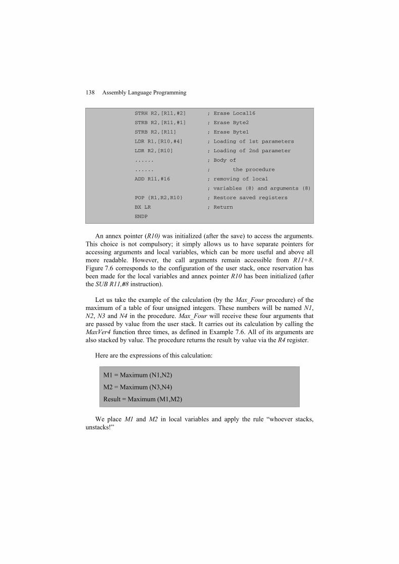
138 Assembly Language Programming
STRH R2,[R11,#2] ; Erase Local16
STRB R2,[R11,#1] ; Erase Byte2
STRB R2,[R11] ; Erase Byte1
LDR R1,[R10,#4] ; Loading of 1st parameters
LDR R2,[R10] ; Loading of 2nd parameter
...... ; Body of
...... ; the procedure
ADD R11,#16 ; removing of local
; variables (8) and arguments (8)
POP {R1,R2,R10} ; Restore saved registers
BX LR ; Return
ENDP
An annex pointer (R10) was initialized (after the save) to access the arguments.This choice is not compulsory; it simply allows us to have separate pointers foraccessing arguments and local variables, which can be more useful and above allmore readable. However, the call arguments remain accessible from R11+8.Figure 7.6 corresponds to the configuration of the user stack, once reservation hasbeen made for the local variables and annex pointer R10 has been initialized (afterthe SUB R11,#8 instruction).
Let us take the example of the calculation (by the Max_Four procedure) of themaximum of a table of four unsigned integers. These numbers will be named N1,N2, N3 and N4 in the procedure. Max_Four will receive these four arguments thatare passed by value from the user stack. It carries out its calculation by calling theMaxVer4 function three times, as defined in Example 7.6. All of its arguments arealso stacked by value. The procedure returns the result by value via the R4 register.
Here are the expressions of this calculation:
M1 = Maximum (N1,N2)
M2 = Maximum (N3,N4)
Result = Maximum (M1,M2)
We place M1 and M2 in local variables and apply the rule “whoever stacks,unstacks!”
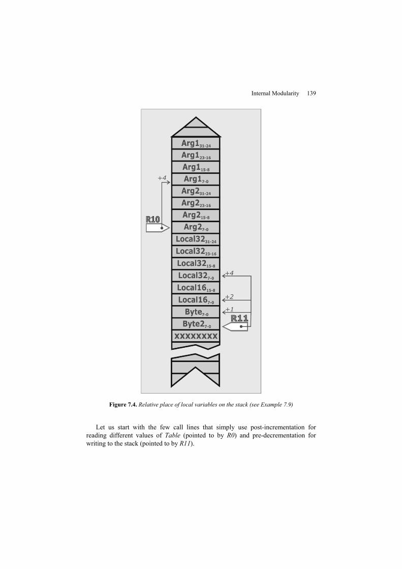
Internal Modularity 139
Figure 7.4. Relative place of local variables on the stack (see Example 7.9)
Let us start with the few call lines that simply use post-incrementation forreading different values of Table (pointed to by R0) and pre-decrementation forwriting to the stack (pointed to by R11).
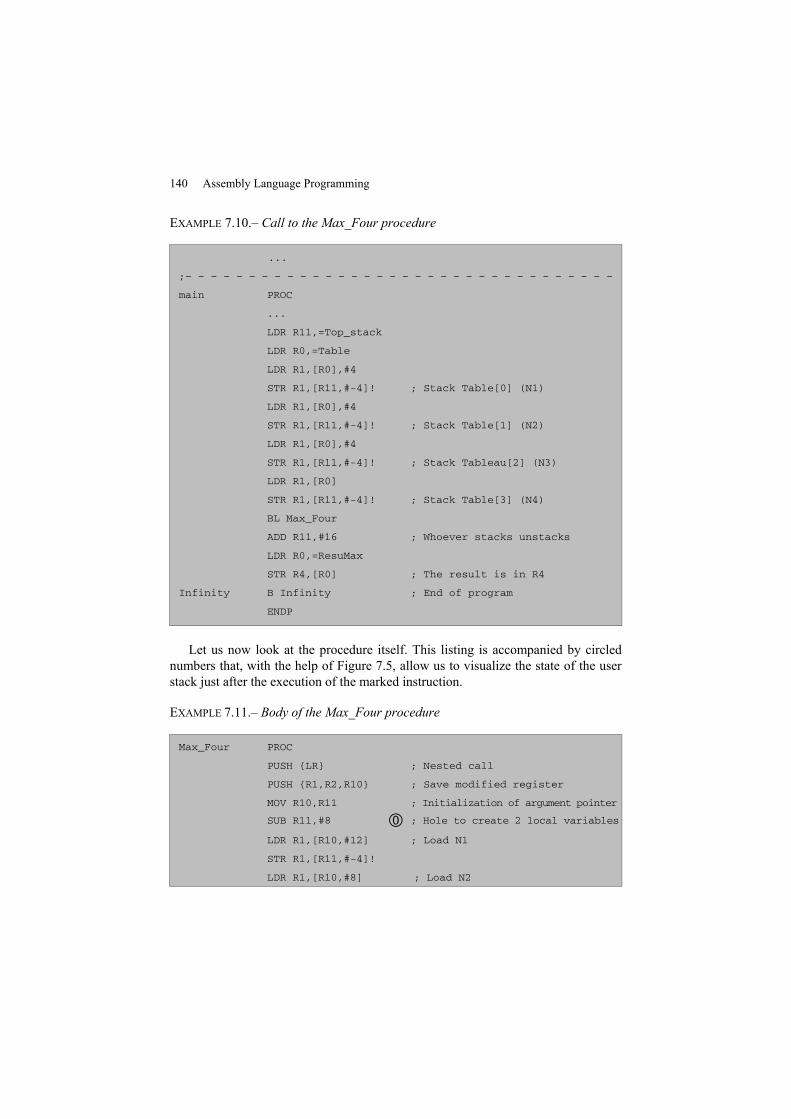
140 Assembly Language Programming
EXAMPLE 7.10.– Call to the Max_Four procedure
...
;– – – – – – – – – – – – – – – – – – – – – – – – – – – – – – – – – –
main PROC
...
LDR R11,=Top_stack
LDR R0,=Table
LDR R1,[R0],#4
STR R1,[R11,#-4]! ; Stack Table[0] (N1)
LDR R1,[R0],#4
STR R1,[R11,#-4]! ; Stack Table[1] (N2)
LDR R1,[R0],#4
STR R1,[R11,#-4]! ; Stack Tableau[2] (N3)
LDR R1,[R0]
STR R1,[R11,#-4]! ; Stack Table[3] (N4)
BL Max_Four
ADD R11,#16 ; Whoever stacks unstacks
LDR R0,=ResuMax
STR R4,[R0] ; The result is in R4
Infinity B Infinity ; End of program
ENDP
Let us now look at the procedure itself. This listing is accompanied by circlednumbers that, with the help of Figure 7.5, allow us to visualize the state of the userstack just after the execution of the marked instruction.
EXAMPLE 7.11.– Body of the Max_Four procedure
Max_Four PROC
PUSH {LR} ; Nested call
PUSH {R1,R2,R10} ; Save modified register
MOV R10,R11 ; Initialization of argument pointer
SUB R11,#8 ; Hole to create 2 local variables
LDR R1,[R10,#12] ; Load N1
STR R1,[R11,#-4]!
LDR R1,[R10,#8] ; Load N2
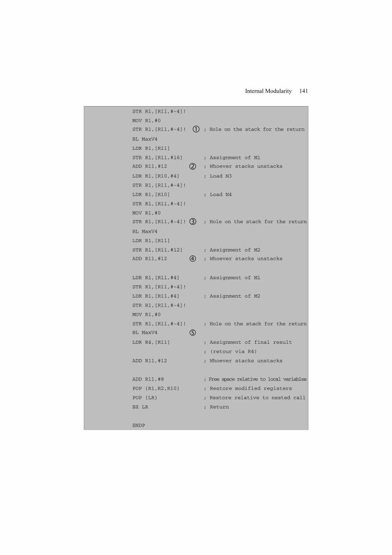
Internal Modularity 141
STR R1,[R11,#-4]!
MOV R1,#0
STR R1,[R11,#-4]! ; Hole on the stack for the return
BL MaxV4
LDR R1,[R11]
STR R1,[R11,#16] ; Assignment of M1
ADD R11,#12 ; Whoever stacks unstacks
LDR R1,[R10,#4] ; Load N3
STR R1,[R11,#-4]!
LDR R1,[R10] ; Load N4
STR R1,[R11,#-4]!
MOV R1,#0
STR R1,[R11,#-4]! ; Hole on the stack for the return
BL MaxV4
LDR R1,[R11]
STR R1,[R11,#12] ; Assignment of M2
ADD R11,#12 ; Whoever stacks unstacks
LDR R1,[R11,#4] ; Assignment of M1
STR R1,[R11,#-4]!
LDR R1,[R11,#4] ; Assignment of M2
STR R1,[R11,#-4]!
MOV R1,#0
STR R1,[R11,#-4]! ; Hole on the stack for the return
BL MaxV4
LDR R4,[R11] ; Assignment of final result
; (retour via R4)
ADD R11,#12 ; Whoever stacks unstacks
ADD R11,#8 ; Free space relative to local variables
POP {R1,R2,R10} ; Restore modified registers
POP {LR} ; Restore relative to nested call
BX LR ; Return
ENDP
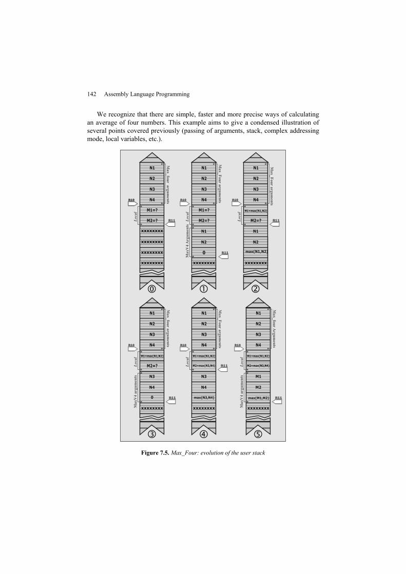
142 Assembly Language Programming
We recognize that there are simple, faster and more precise ways of calculatingan average of four numbers. This example aims to give a condensed illustration ofseveral points covered previously (passing of arguments, stack, complex addressingmode, local variables, etc.).
xxxxxxxx
xxxxxxxx
xxxxxxxx
xxxxxxxx
N1
N2
N3
M1=?
M2=?
N4R10R10
R11R11
R11R11
Lo
ca
l
Ma
x_
fou
ra
rgu
men
ts
xxxxxxxx
0
N2
N1
N1
N2
N3
M1=?
M2=?
N4R10R10
Lo
ca
lM
ax
_F
ou
ra
rgu
men
tsM
ax
V4
Arg
um
ents
R11R11
xxxxxxxx
max(N1,N2)
N2
N1
N1
N2
N3
M1=max(N1,N2)
M2=?
N4R10R10
Lo
ca
l
Ma
x_
Fo
ur
arg
um
ents
R11R11
xxxxxxxx
0
N4
N3
N1
N2
N3
M1=max(N1,N2)
M2=?
N4R10R10
R11R11
R10R10
xxxxxxxx
max(N3,N4)
N4
N3
N1
N2
N3
M1=max(N1,N2)
N4
M2=max(N3,N4)
R11R11
xxxxxxxx
max(M1,M2)
M2
M1
N1
N2
N3
M1=max(N1,N2)
N4R10R10
M2=max(N3,N4)Lo
ca
l
Ma
x_
fou
ra
rgu
men
ts
Ma
xV
4a
rgu
men
ts
Lo
ca
lM
ax
_F
ou
ra
rgu
men
ts
Lo
ca
l
Ma
x_
fou
rA
rgu
men
ts
Ma
xV
4a
rgu
men
ts
Figure 7.5. Max_Four: evolution of the user stack
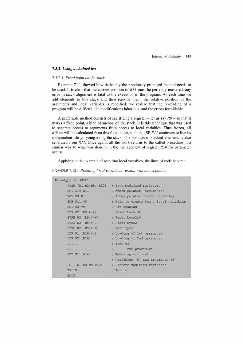
Internal Modularity 143
7.3.2. Using a chained list
7.3.2.1. Fixed point on the stack
Example 7.11 showed how delicately the previously proposed method needs tobe used. It is clear that the current position of R11 must be perfectly mastered: anyerror in stack alignment is fatal to the execution of the program. As each time weadd elements to this stack and then remove them, the relative position of thearguments and local variables is modified, we realize that the re-reading of aprogram will be difficult, the modifications laborious, and the errors formidable.
A preferable method consists of sacrificing a register – let us say R9 – so that itmarks a fixed point, a kind of anchor, on the stack. It is this technique that was usedto separate access to arguments from access to local variables. Thus frozen, alloffsets will be calculated from this fixed point, such that SP R11 continues to live itsindependent life yo-yoing along the stack. The position of stacked elements is alsoseparated from R11. Once again, all the work returns to the called procedure in asimilar way to what was done with the management of register R10 for parameteraccess.
Applying to the example of resetting local variables, the lines of code become:
EXAMPLE 7.12.– Resetting local variables: version with annex pointer
Erase2_Local PROC
PUSH {R1,R2,R9, R10} ; Save modified registers
MOV R10,R11 ; Annex pointer (arguments)
MOV R9,R11 ; Annex pointer (local variables)
SUB R11,#8 ; Hole to create the 4 local variables
MOV R2,#0 ; For erasing
STR R2,[R9,#-4] ; Reset Local32
STRH R2,[R9,#-6] ; Reset Local16
STRB R2,[R9,#-7] ; Reset Byte2
STRB R2,[R9,#-8] ; Rest Byte1
LDR R1,[R10,#4] ; Loading of 1st parameter
LDR R2,[R10] ; Loading of 2nd parameter
...... ; Body of
...... ; the procedure
ADD R11,#16 ; Removing of local
; variables (8) and arguments (8)
POP {R1,R2,R9,R10} ; Restore modified registers
BX LR ; Return
ENDP
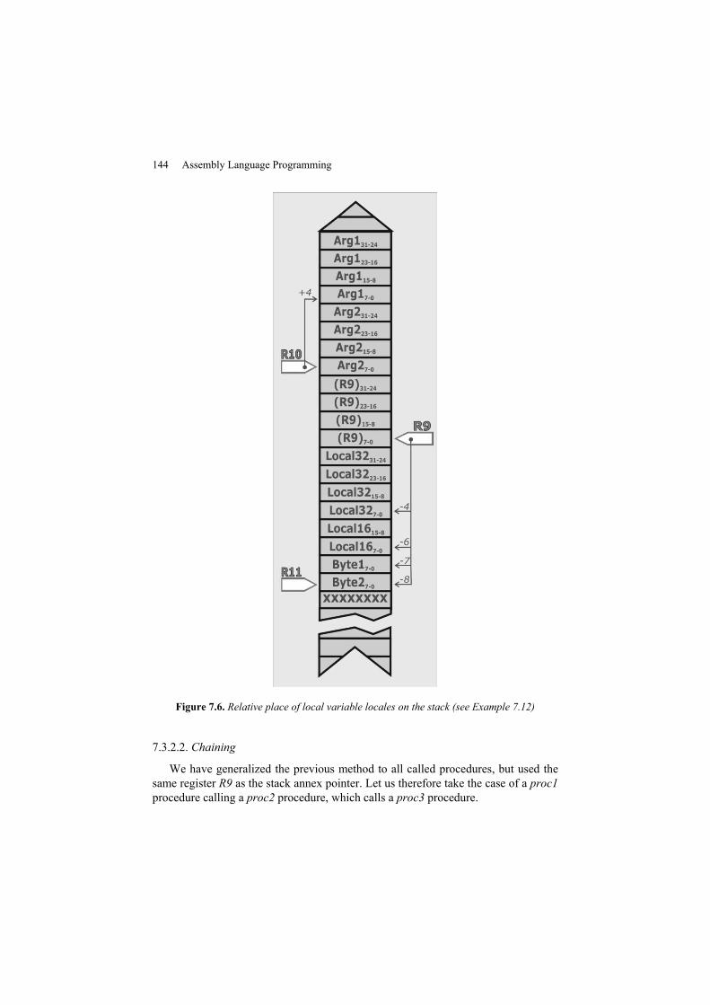
144 Assembly Language Programming
Figure 7.6. Relative place of local variable locales on the stack (see Example 7.12)
7.3.2.2. Chaining
We have generalized the previous method to all called procedures, but used thesame register R9 as the stack annex pointer. Let us therefore take the case of a proc1procedure calling a proc2 procedure, which calls a proc3 procedure.
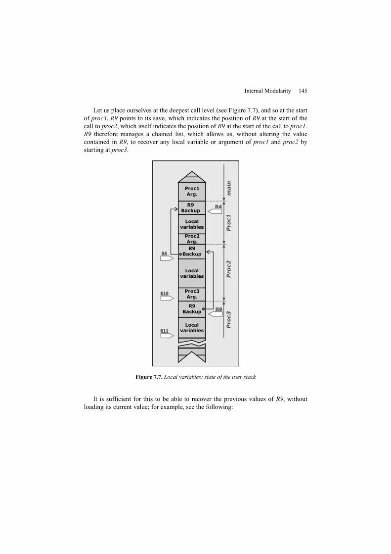
Internal Modularity 145
Let us place ourselves at the deepest call level (see Figure 7.7), and so at the startof proc3. R9 points to its save, which indicates the position of R9 at the start of thecall to proc2, which itself indicates the position of R9 at the start of the call to proc1.R9 therefore manages a chained list, which allows us, without altering the valuecontained in R9, to recover any local variable or argument of proc1 and proc2 bystarting at proc3.
Figure 7.7. Local variables: state of the user stack
It is sufficient for this to be able to recover the previous values of R9, withoutloading its current value; for example, see the following:
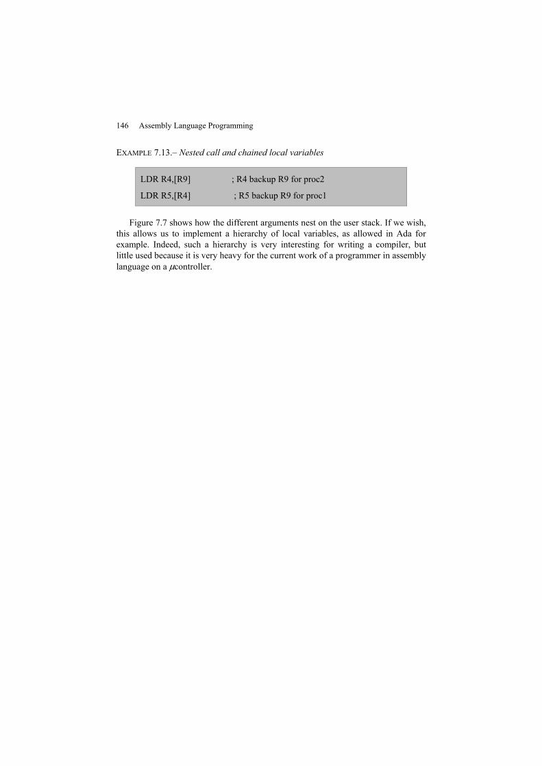
146 Assembly Language Programming
EXAMPLE 7.13.– Nested call and chained local variables
LDR R4,[R9] ; R4 backup R9 for proc2
LDR R5,[R4] ; R5 backup R9 for proc1
Figure 7.7 shows how the different arguments nest on the user stack. If we wish,this allows us to implement a hierarchy of local variables, as allowed in Ada forexample. Indeed, such a hierarchy is very interesting for writing a compiler, butlittle used because it is very heavy for the current work of a programmer in assemblylanguage on a μcontroller.
Chapter 8
Managing Exceptions
Understanding of exception mechanisms is an essential step when it comes tocomputer hardware. The core of a μcontroller is responsible for the execution ofalgorithms, task management and calculations necessary for the project, but all ofthis organization would be useless if it was not accompanied by the possibility ofinterfacing (in the electronic sense) with the physical process that it has to manage.As was explained in Chapter 1, it is the responsibility of the μcontroller designer(and not the Advanced RISC Machine or ARM) to develop these peripherals. Thesecan be thought of as micromachines that are independent of the core and performspecific tasks (counting time, converting an analog signal into its numericalequivalent, periodically generating a square signal, etc.). Their preferred means ofcommunication is the interrupt. By this specific mechanism, the micromachinesignals to Cortex-M3, asynchronously with the current code execution, that it hasfinished its task and that Cortex-M3should therefore respond accordingly.
A similar mechanism is engaged when, during the running of a code sequence, a“serious” event occurs and its processing requires a particular regime. As anexample, let us take the case of an attempt to read the contents of a memory addressthat, for some reason, fails. This type of event is strictly specific to the functioningof the core and is usually launched synchronously with an instruction. It is thenpossible to speak of software traps.
Finally, another type of communication can arise, which concerns the launch of areset or a Non-Maskable Interrupt (NMI). These two events are generallytransmitted by specific external pins of the processor and can be thought of as“emergency stops”.
148 Assembly Language Programming
Interrupts, traps, Reset and NMI come under the generic term exceptions. Thetechnique used to respond to these different cases of “exception” is similar and is thetopic of this chapter. The Nested Vectored Interrupt Controller (NVIC) receivesorders and manages all exceptions, so in this chapter, we will detail many of thisunit’s registers.
8.1. What happens during Reset?
Before describing these mechanisms and what consequences they imply at aprogramming level in greater detail, let us look at the case of Reset. This is the mostserious and most inescapable event (or exception, to be more precise) that canhappen to any μprocessor. A system Reset can have different origins. In the case ofCortex-M3, these can be:
– exterior, meaning that a circuit particular pin that must, by default, be at a highlogic level has passed to a low level;
– launched by a watchdog1;
– launched by software by setting the SYSRESETREQ bit of the ApplicationInterrupt and Reset Control Register (AIRCR) in the NVIC to 1.
Reset also corresponds to a “cold start”, or power-up of the circuit. If itcorresponds to setting the Reset pin of the circuit to a lower level (known as a softreset, corresponding in practice to the user pressing a button wired to this pin), itgenerally does not bode well for the progress of the application running on theprocessor.
During a Reset phase, the processor starts by reinitializing all registers. In thedocumentation, we find the value taken by each register following a Reset. Thisinitialization puts the processor in privileged Thread mode. Then Cortex-M3 readsthe contents of address 0x00000000 (the lowest memory mapping address) to assignit to register R13. Once this has been done, it initializes the stack pointer. This firstassignment is imperative because an exception can occur at any time and becausethe treatment of this exception, as we will see later, requires access to the systemstack. The processor must therefore be in a position to process an exception andconsequently must have a valid stack pointer. The memory address recorded in these4 bytes must correspond to the top of a memory zone with read/write access. In athird stage, Cortex-M3 reads the contents of the next word, namely the contents ofaddresses 0x00000004 to 0x00000007. This word will be used in the initialization of
1 The watchdogs are bits that must (when these units are engaged) be periodically set to 1.This mechanism allows the µcontroller to ensure that the running program is not blocked inan infinite loop, among other things.
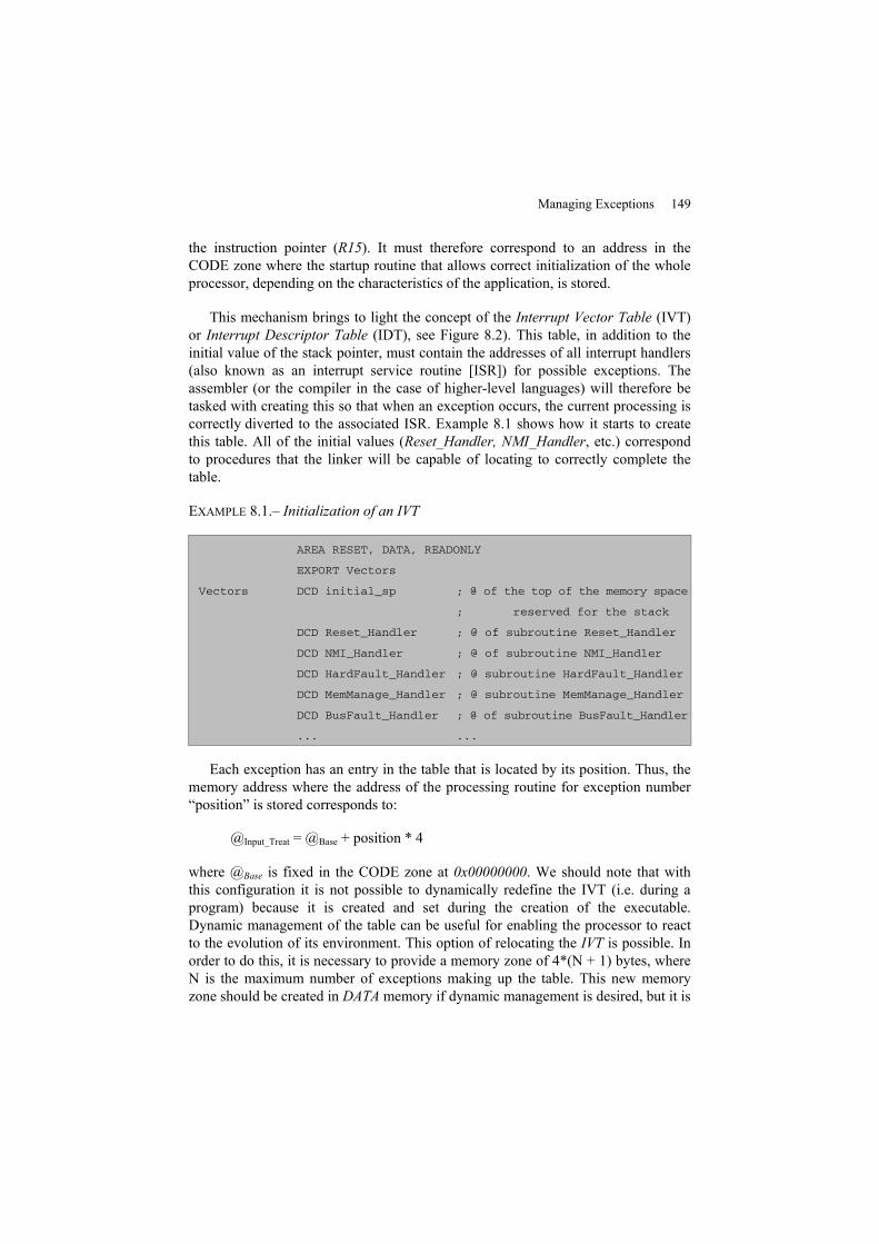
Managing Exceptions 149
the instruction pointer (R15). It must therefore correspond to an address in theCODE zone where the startup routine that allows correct initialization of the wholeprocessor, depending on the characteristics of the application, is stored.
This mechanism brings to light the concept of the Interrupt Vector Table (IVT)or Interrupt Descriptor Table (IDT), see Figure 8.2). This table, in addition to theinitial value of the stack pointer, must contain the addresses of all interrupt handlers(also known as an interrupt service routine [ISR]) for possible exceptions. Theassembler (or the compiler in the case of higher-level languages) will therefore betasked with creating this so that when an exception occurs, the current processing iscorrectly diverted to the associated ISR. Example 8.1 shows how it starts to createthis table. All of the initial values (Reset_Handler, NMI_Handler, etc.) correspondto procedures that the linker will be capable of locating to correctly complete thetable.
EXAMPLE 8.1.– Initialization of an IVT
AREA RESET, DATA, READONLY
EXPORT Vectors
Vectors DCD initial_sp ; @ of the top of the memory space
; reserved for the stack
DCD Reset_Handler ; @ of subroutine Reset_Handler
DCD NMI_Handler ; @ of subroutine NMI_Handler
DCD HardFault_Handler ; @ subroutine HardFault_Handler
DCD MemManage_Handler ; @ subroutine MemManage_Handler
DCD BusFault_Handler ; @ of subroutine BusFault_Handler
... ...
Each exception has an entry in the table that is located by its position. Thus, thememory address where the address of the processing routine for exception number“position” is stored corresponds to:
@Input_Treat = @Base + position * 4
where @Base is fixed in the CODE zone at 0x00000000. We should note that withthis configuration it is not possible to dynamically redefine the IVT (i.e. during aprogram) because it is created and set during the creation of the executable.Dynamic management of the table can be useful for enabling the processor to reactto the evolution of its environment. This option of relocating the IVT is possible. Inorder to do this, it is necessary to provide a memory zone of 4*(N + 1) bytes, whereN is the maximum number of exceptions making up the table. This new memoryzone should be created in DATA memory if dynamic management is desired, but it is
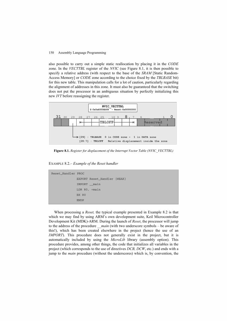
150 Assembly Language Programming
also possible to carry out a simple static reallocation by placing it in the CODEzone. In the VECTTBL register of the NVIC (see Figure 8.1, it is then possible tospecify a relative address (with respect to the base of the SRAM [Static Random-Access Memory] or CODE zone according to the choice fixed by the TBLBASE bit)for this new table. This manipulation calls for a lot of caution, particularly regardingthe alignment of addresses in this zone. It must also be guaranteed that the switchingdoes not put the processor in an ambiguous situation by perfectly initializing thisnew IVT before reassigning the register.
Figure 8.1. Register for displacement of the Interrupt Vector Table (NVIC_VECTTBL)
EXAMPLE 8.2.– Example of the Reset handler
Reset_Handler PROC
EXPORT Reset_Handler [WEAK]
IMPORT __main
LDR R0, =main
BX R0
ENDP
When processing a Reset, the typical example presented in Example 8.2 is thatwhich we may find by using ARM’s own development suite, Keil MicrocontrollerDevelopment Kit (MDK)-ARM. During the launch of Reset, the processor will jumpto the address of the procedure __main (with two underscore symbols – be aware ofthis!), which has been created elsewhere in the project (hence the use of anIMPORT). This procedure does not generally exist in the project, but it isautomatically included by using the MicroLib library (assembly option). Thisprocedure provides, among other things, the code that initializes all variables in theproject (which corresponds to the use of directives DCB, DCW, etc.) and ends with ajump to the main procedure (without the underscores) which is, by convention, the
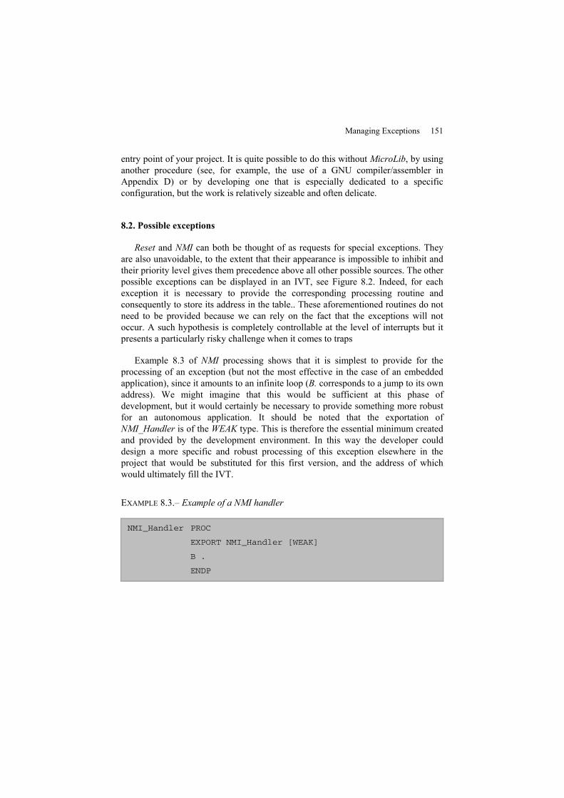
Managing Exceptions 151
entry point of your project. It is quite possible to do this without MicroLib, by usinganother procedure (see, for example, the use of a GNU compiler/assembler inAppendix D) or by developing one that is especially dedicated to a specificconfiguration, but the work is relatively sizeable and often delicate.
8.2. Possible exceptions
Reset and NMI can both be thought of as requests for special exceptions. Theyare also unavoidable, to the extent that their appearance is impossible to inhibit andtheir priority level gives them precedence above all other possible sources. The otherpossible exceptions can be displayed in an IVT, see Figure 8.2. Indeed, for eachexception it is necessary to provide the corresponding processing routine andconsequently to store its address in the table.. These aforementioned routines do notneed to be provided because we can rely on the fact that the exceptions will notoccur. A such hypothesis is completely controllable at the level of interrupts but itpresents a particularly risky challenge when it comes to traps
Example 8.3 of NMI processing shows that it is simplest to provide for theprocessing of an exception (but not the most effective in the case of an embeddedapplication), since it amounts to an infinite loop (B. corresponds to a jump to its ownaddress). We might imagine that this would be sufficient at this phase ofdevelopment, but it would certainly be necessary to provide something more robustfor an autonomous application. It should be noted that the exportation ofNMI_Handler is of the WEAK type. This is therefore the essential minimum createdand provided by the development environment. In this way the developer coulddesign a more specific and robust processing of this exception elsewhere in theproject that would be substituted for this first version, and the address of whichwould ultimately fill the IVT.
EXAMPLE 8.3.– Example of a NMI handler
NMI_Handler PROC
EXPORT NMI_Handler [WEAK]
B .
ENDP
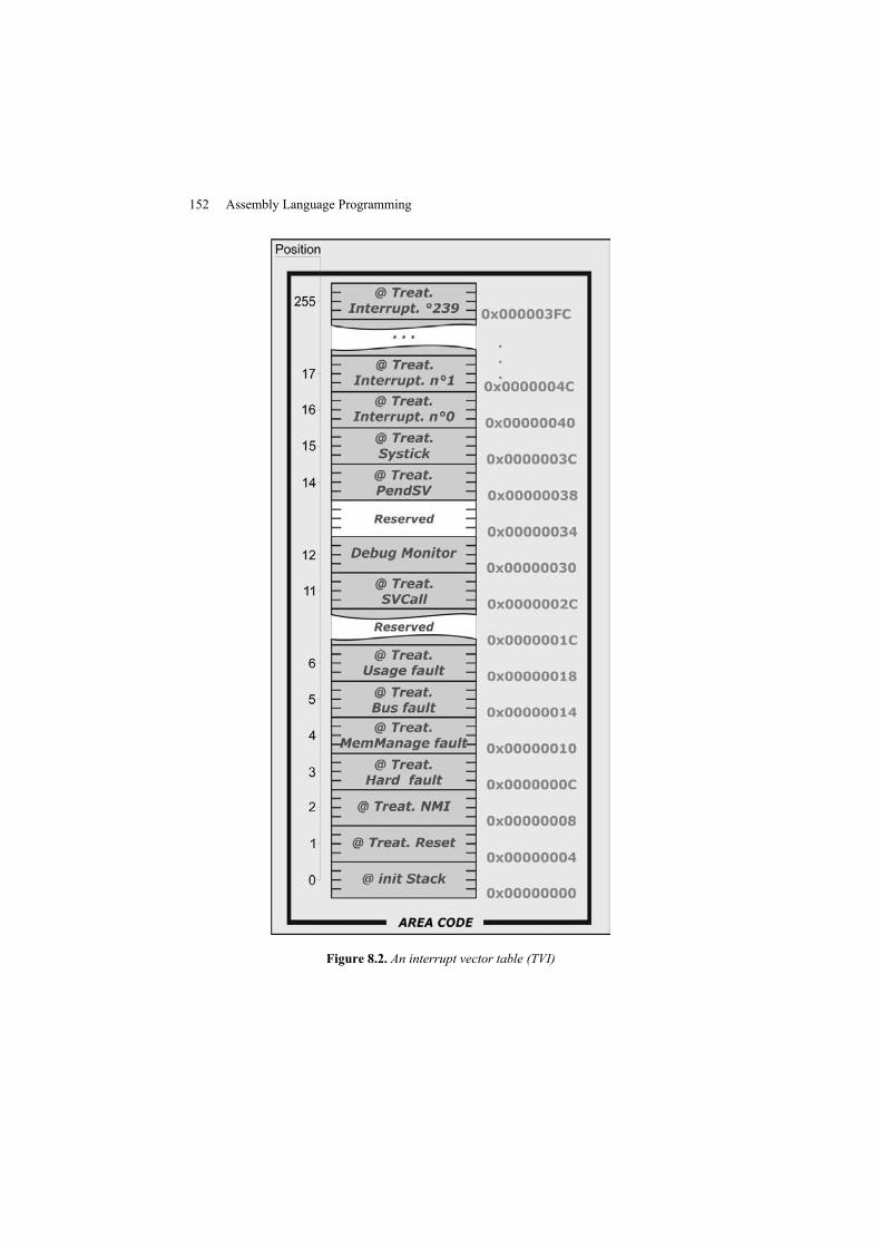
152 Assembly Language Programming
Figure 8.2. An interrupt vector table (TVI)
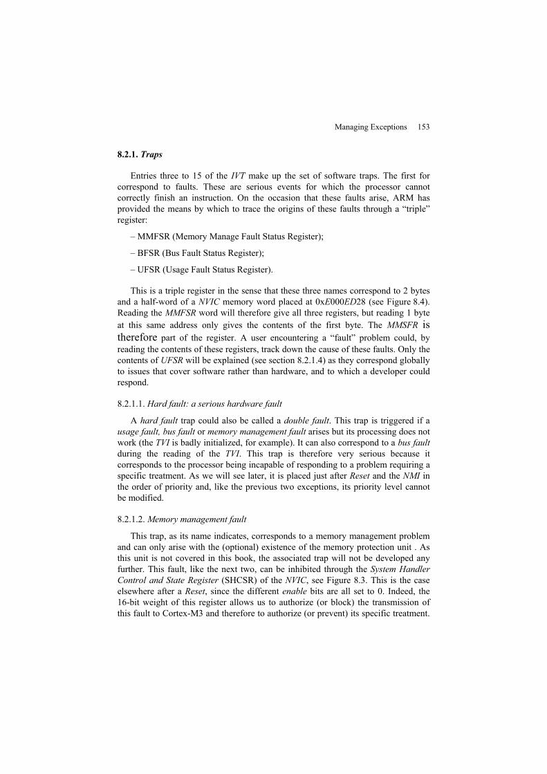
Managing Exceptions 153
8.2.1. Traps
Entries three to 15 of the IVT make up the set of software traps. The first forcorrespond to faults. These are serious events for which the processor cannotcorrectly finish an instruction. On the occasion that these faults arise, ARM hasprovided the means by which to trace the origins of these faults through a “triple”register:
– MMFSR (Memory Manage Fault Status Register);
– BFSR (Bus Fault Status Register);
– UFSR (Usage Fault Status Register).
This is a triple register in the sense that these three names correspond to 2 bytesand a half-word of a NVIC memory word placed at 0xE000ED28 (see Figure 8.4).Reading the MMFSR word will therefore give all three registers, but reading 1 byteat this same address only gives the contents of the first byte. The MMSFR istherefore part of the register. A user encountering a “fault” problem could, byreading the contents of these registers, track down the cause of these faults. Only thecontents of UFSR will be explained (see section 8.2.1.4) as they correspond globallyto issues that cover software rather than hardware, and to which a developer couldrespond.
8.2.1.1. Hard fault: a serious hardware fault
A hard fault trap could also be called a double fault. This trap is triggered if ausage fault, bus fault or memory management fault arises but its processing does notwork (the TVI is badly initialized, for example). It can also correspond to a bus faultduring the reading of the TVI. This trap is therefore very serious because itcorresponds to the processor being incapable of responding to a problem requiring aspecific treatment. As we will see later, it is placed just after Reset and the NMI inthe order of priority and, like the previous two exceptions, its priority level cannotbe modified.
8.2.1.2.Memory management fault
This trap, as its name indicates, corresponds to a memory management problemand can only arise with the (optional) existence of the memory protection unit . Asthis unit is not covered in this book, the associated trap will not be developed anyfurther. This fault, like the next two, can be inhibited through the System HandlerControl and State Register (SHCSR) of the NVIC, see Figure 8.3. This is the caseelsewhere after a Reset, since the different enable bits are all set to 0. Indeed, the16-bit weight of this register allows us to authorize (or block) the transmission ofthis fault to Cortex-M3 and therefore to authorize (or prevent) its specific treatment.
154 Assembly Language Programming
However, we cannot solve the problem by inhibiting it. Similarly the 0 (or 13)-bitsweight allow us to find out, as we will see later in the chapter, whether the specifictreatment of the exception is active (or pending). As these last two bits have writeaccess, it is possible to artificially trigger exceptions by setting these bits to 1. It isrecommended that act cautiously in doing this, however, insofar as the save contextis not always guaranteed.
Figure 8.3. System Handler Control and State Register (NVIC_SHCSR)
8.2.1.3. Bus fault
With this trap, problems that are potentially present in the development phasebegin to appear. This corresponds to it being impossible for the processor to retrievean instruction (prefetch abort) or carry out reading/writing of a datum (data abort).The typical case in which Cortex-M3 falls into this trap is that of bad pointermanagement (and so indirect addressing), where the virtually pointed address (thecontents of the indirection register) does not correspond to a valid data address.Another common problem is the bad use of a peripheral that, for example, tries toretrieve a word so that it can only provide one byte. In certain cases, the BFAR (BusFault Address Register) preserves the memory address that produced the fault. Bit17 of the SHCSR register allows us to validate or invalidate this trap and bits 14 and1 allow us to determine its activity state (active or pending).
Managing Exceptions 155
8.2.1.4. Usage fault
This last fault, of which a report on what triggers it is the subject of the 16-bitUFSR, is a fault that, as opposed to a bus fault, is more concerned with softwarethan hardware problems. It can therefore occur in the deployment phase (not only inthe development phase) so it is important to provide treatment for it and to see howit can be caused:
– division by zero: in the case of floating point numbers, it is possible tode-normalize the result to return a value corresponding to infinity. In integerarithmetic, such an operation poses an unsolvable problem. So, the processorindicates this fault and switches the weight 9 bit (DIVBYZERO) of UFSR to 1;
– unalignment: as we have seen, it is possible to access unaligned data. Thisoption comes with limitations, however, and when we violate these constraints thetrap is triggered and bit 8 (UNALIGNED) is activated. It is also activated ifunaligned access is prohibited and such access is attempted;
– access to a coprocessor: the Cortex-M3 set has several instructions for apotential coprocessor. If no such unit is present, the response is a usage fault andbit 3 (NOCP) switches to 1. By finding this bit, the treatment routine can be writtento offer an emulation of this coprocessor (which allows us to augment the portabilityof the code to different types of processors);
– impossible return: here this means an attempt to load the program counter (PC)pointer with an illegal value during the return from an exception. The details ofpossible values are given in section 8.4. Bit 2 (INVPC) switches to 1;
– invalid state: the T bit of the EPSR (Execution Program Status Register) allowsus to distinguish, in the general ARM architectures, the switch from ARM mode toThumb mode. As Cortex-M3 only supports Thumb mode, any attempt to switch toARM mode is sanctioned by this fault, with bit 1 (INVSTATE) being activated. Thisproblem can happen accidentally by forcing the value of PC with an even value (sothe least significant bit (LSB) is at 0), during a jump or procedure return (BX LR) forexample. Indeed, in coding jump instructions (see section 5.6) when the LSB is at 0,the processor as well as the branch must switch to ARM mode, which is impossiblefor Cortex-M3;
– undefined instruction: the last case that provokes this fault is when bit 0(UNDEFINSTR) is set to 1. In this case, the PC points to an instruction that is notdecodable by the core. The most common case is a jump to an address that is valid,but does not contain the correct code (a Literal Pool, for example).
A usage fault can be deactivated. To do this, we set bit 18 of the SHCSR to 0.Bits 12 and 3 of this register allow knowledge of the activity state (active orpending).
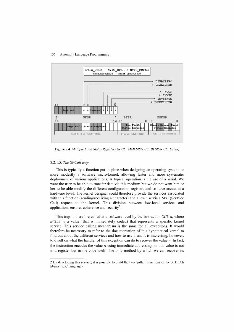
156 Assembly Language Programming
Figure 8.4. Multiple Fault Status Registers (NVIC_MMFSR/NVIC_BFSR/NVIC_UFSR)
8.2.1.5. The SVCall trap
This is typically a function put in place when designing an operating system, ormore modestly a software micro-kernel, allowing faster and more systematicdeployment of various applications. A typical operation is the use of a serial. Wewant the user to be able to transfer data via this medium but we do not want him orher to be able modify the different configuration registers and so have access at ahardware level. The kernel designer could therefore provide the services associatedwith this function (sending/receiving a character) and allow use via a SVC (SerViceCall) request to the kernel. This division between low-level services andapplications ensures coherence and security2.
This trap is therefore called at a software level by the instruction SCV n, wheren<255 is a value (that is immediately coded) that represents a specific kernelservice. This service calling mechanism is the same for all exceptions. It wouldtherefore be necessary to refer to the documentation of this hypothetical kernel tofind out about the different services and how to use them. It is interesting, however,to dwell on what the handler of this exception can do to recover the value n. In fact,the instruction encodes the value n using immediate addressing, so this value is notin a register but in the code itself. The only method by which we can recover its
2 By developing this service, it is possible to build the two “pillar” functions of the STDIO.hlibrary (in C language).
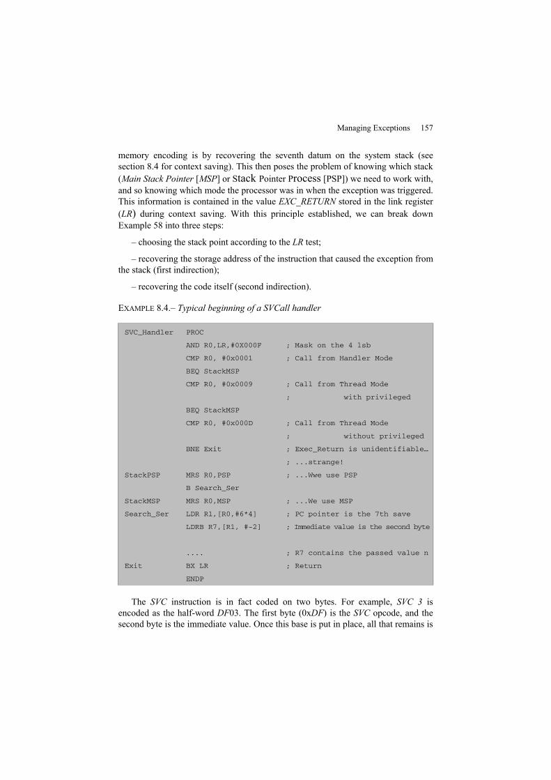
Managing Exceptions 157
memory encoding is by recovering the seventh datum on the system stack (seesection 8.4 for context saving). This then poses the problem of knowing which stack(Main Stack Pointer [MSP] or Stack Pointer Process [PSP]) we need to work with,and so knowing which mode the processor was in when the exception was triggered.This information is contained in the value EXC_RETURN stored in the link register(LR) during context saving. With this principle established, we can break downExample 58 into three steps:
– choosing the stack point according to the LR test;
– recovering the storage address of the instruction that caused the exception fromthe stack (first indirection);
– recovering the code itself (second indirection).
EXAMPLE 8.4.– Typical beginning of a SVCall handler
SVC_Handler PROC
AND R0,LR,#0X000F ; Mask on the 4 lsb
CMP R0, #0x0001 ; Call from Handler Mode
BEQ StackMSP
CMP R0, #0x0009 ; Call from Thread Mode
; with privileged
BEQ StackMSP
CMP R0, #0x000D ; Call from Thread Mode
; without privileged
BNE Exit ; Exec_Return is unidentifiable…
; ...strange!
StackPSP MRS R0,PSP ; ...Wwe use PSP
B Search_Ser
StackMSP MRS R0,MSP ; ...We use MSP
Search_Ser LDR R1,[R0,#6*4] ; PC pointer is the 7th save
LDRB R7,[R1, #-2] ; Immediate value is the second byte
.... ; R7 contains the passed value n
Exit BX LR ; Return
ENDP
The SVC instruction is in fact coded on two bytes. For example, SVC 3 isencoded as the half-word DF03. The first byte (0xDF) is the SVC opcode, and thesecond byte is the immediate value. Once this base is put in place, all that remains is
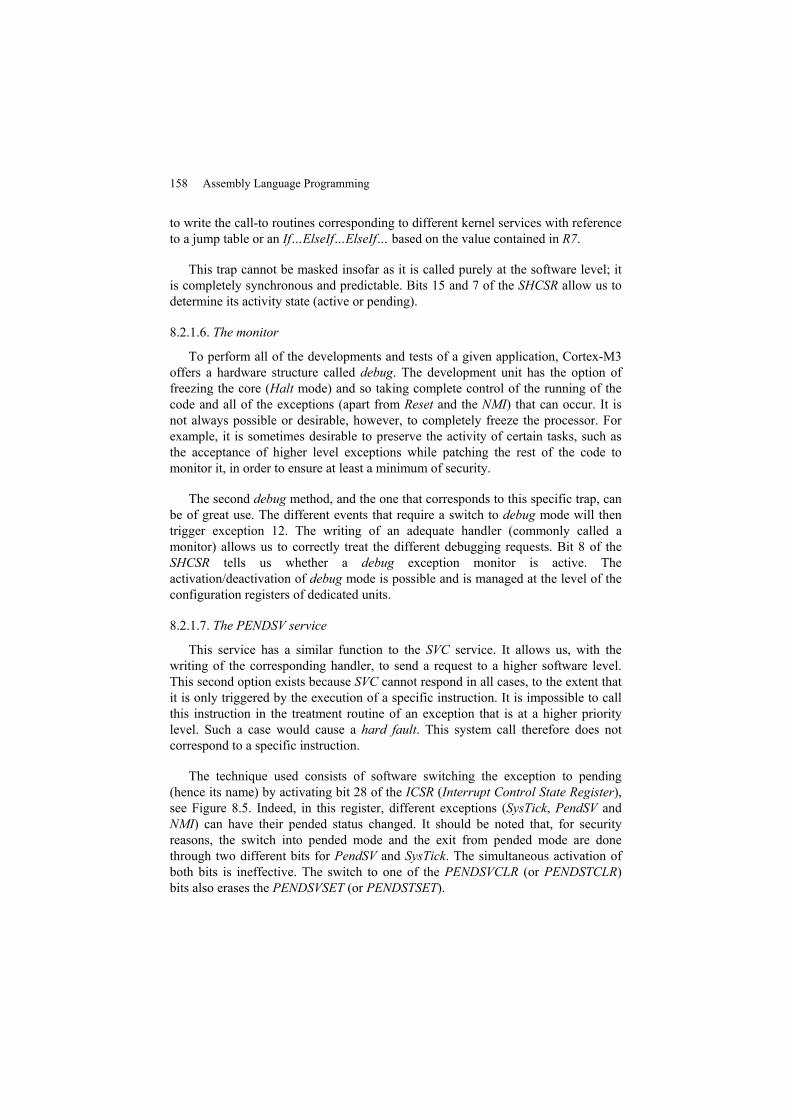
158 Assembly Language Programming
to write the call-to routines corresponding to different kernel services with referenceto a jump table or an If…ElseIf…ElseIf… based on the value contained in R7.
This trap cannot be masked insofar as it is called purely at the software level; itis completely synchronous and predictable. Bits 15 and 7 of the SHCSR allow us todetermine its activity state (active or pending).
8.2.1.6. The monitor
To perform all of the developments and tests of a given application, Cortex-M3offers a hardware structure called debug. The development unit has the option offreezing the core (Halt mode) and so taking complete control of the running of thecode and all of the exceptions (apart from Reset and the NMI) that can occur. It isnot always possible or desirable, however, to completely freeze the processor. Forexample, it is sometimes desirable to preserve the activity of certain tasks, such asthe acceptance of higher level exceptions while patching the rest of the code tomonitor it, in order to ensure at least a minimum of security.
The second debug method, and the one that corresponds to this specific trap, canbe of great use. The different events that require a switch to debug mode will thentrigger exception 12. The writing of an adequate handler (commonly called amonitor) allows us to correctly treat the different debugging requests. Bit 8 of theSHCSR tells us whether a debug exception monitor is active. Theactivation/deactivation of debug mode is possible and is managed at the level of theconfiguration registers of dedicated units.
8.2.1.7. The PENDSV service
This service has a similar function to the SVC service. It allows us, with thewriting of the corresponding handler, to send a request to a higher software level.This second option exists because SVC cannot respond in all cases, to the extent thatit is only triggered by the execution of a specific instruction. It is impossible to callthis instruction in the treatment routine of an exception that is at a higher prioritylevel. Such a case would cause a hard fault. This system call therefore does notcorrespond to a specific instruction.
The technique used consists of software switching the exception to pending(hence its name) by activating bit 28 of the ICSR (Interrupt Control State Register),see Figure 8.5. Indeed, in this register, different exceptions (SysTick, PendSV andNMI) can have their pended status changed. It should be noted that, for securityreasons, the switch into pended mode and the exit from pended mode are donethrough two different bits for PendSV and SysTick. The simultaneous activation ofboth bits is ineffective. The switch to one of the PENDSVCLR (or PENDSTCLR)bits also erases the PENDSVSET (or PENDSTSET).
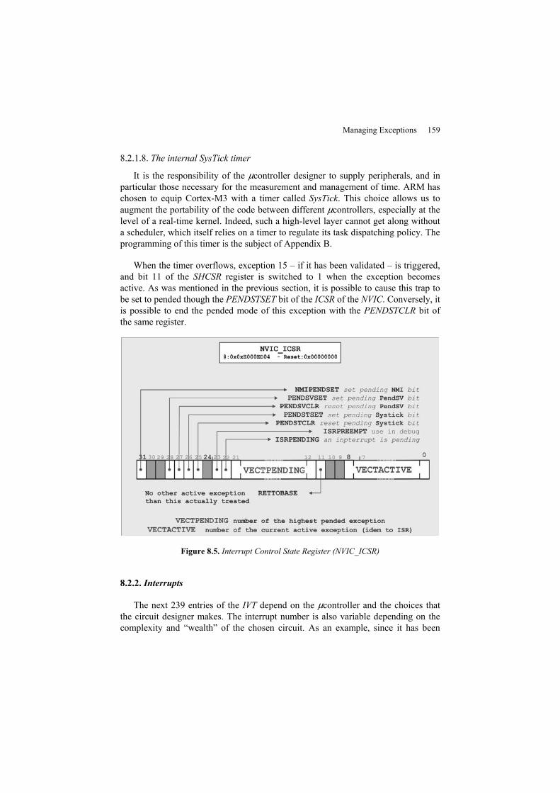
Managing Exceptions 159
8.2.1.8. The internal SysTick timer
It is the responsibility of the μcontroller designer to supply peripherals, and inparticular those necessary for the measurement and management of time. ARM haschosen to equip Cortex-M3 with a timer called SysTick. This choice allows us toaugment the portability of the code between different μcontrollers, especially at thelevel of a real-time kernel. Indeed, such a high-level layer cannot get along withouta scheduler, which itself relies on a timer to regulate its task dispatching policy. Theprogramming of this timer is the subject of Appendix B.
When the timer overflows, exception 15 – if it has been validated – is triggered,and bit 11 of the SHCSR register is switched to 1 when the exception becomesactive. As was mentioned in the previous section, it is possible to cause this trap tobe set to pended though the PENDSTSET bit of the ICSR of the NVIC. Conversely, itis possible to end the pended mode of this exception with the PENDSTCLR bit ofthe same register.
Figure 8.5. Interrupt Control State Register (NVIC_ICSR)
8.2.2. Interrupts
The next 239 entries of the IVT depend on the μcontroller and the choices thatthe circuit designer makes. The interrupt number is also variable depending on thecomplexity and “wealth” of the chosen circuit. As an example, since it has been
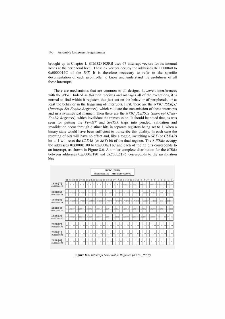
160 Assembly Language Programming
brought up in Chapter 1, STM32F103RB uses 67 interrupt vectors for its internalneeds at the peripheral level. These 67 vectors occupy the addresses 0x00000040 to0x0000014C of the IVT. It is therefore necessary to refer to the specificdocumentation of each μcontroller to know and understand the usefulness of allthese interrupts.
There are mechanisms that are common to all designs, however: interferenceswith the NVIC. Indeed as this unit receives and manages all of the exceptions, it isnormal to find within it registers that just act on the behavior of peripherals, or atleast the behavior in the triggering of interrupts. First, there are the NVIC_ISER[x](Interrupt Set-Enable Registers), which validate the transmission of these interruptsand in a symmetrical manner. Then there are the NVIC_ICER[x] (Interrupt Clear-Enable Registers), which invalidate the transmission. It should be noted that, as wasseen for putting the PendSV and SysTick traps into pended, validation andinvalidation occur through distinct bits in separate registers being set to 1, when abinary state would have been sufficient to transcribe this duality. In each case theresetting of bits will have no effect and, like a toggle, switching a SET (or CLEAR)bit to 1 will reset the CLEAR (or SET) bit of the dual register. The 8 ISERs occupythe addresses 0xE000E100 to 0xE000E11C and each of the 32 bits corresponds toan interrupt, as shown in Figure 8.6. A similar complete distribution for the ICERsbetween addresses 0xE000E180 and 0xE000E19C corresponds to the invalidationbits.
Figure 8.6. Interrupt Set-Enable Register (NVIC_ISER)
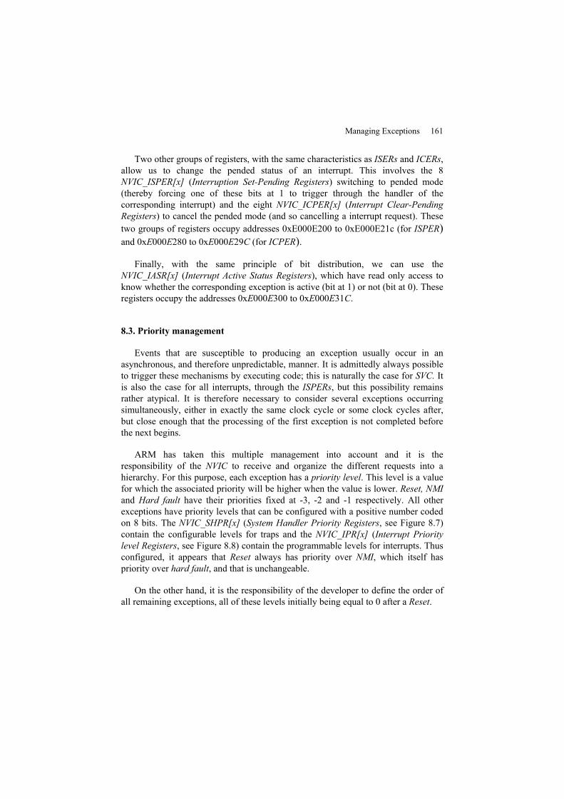
Managing Exceptions 161
Two other groups of registers, with the same characteristics as ISERs and ICERs,allow us to change the pended status of an interrupt. This involves the 8NVIC_ISPER[x] (Interruption Set-Pending Registers) switching to pended mode(thereby forcing one of these bits at 1 to trigger through the handler of thecorresponding interrupt) and the eight NVIC_ICPER[x] (Interrupt Clear-PendingRegisters) to cancel the pended mode (and so cancelling a interrupt request). Thesetwo groups of registers occupy addresses 0xE000E200 to 0xE000E21c (for ISPER)and 0xE000E280 to 0xE000E29C (for ICPER).
Finally, with the same principle of bit distribution, we can use theNVIC_IASR[x] (Interrupt Active Status Registers), which have read only access toknow whether the corresponding exception is active (bit at 1) or not (bit at 0). Theseregisters occupy the addresses 0xE000E300 to 0xE000E31C.
8.3. Priority management
Events that are susceptible to producing an exception usually occur in anasynchronous, and therefore unpredictable, manner. It is admittedly always possibleto trigger these mechanisms by executing code; this is naturally the case for SVC. Itis also the case for all interrupts, through the ISPERs, but this possibility remainsrather atypical. It is therefore necessary to consider several exceptions occurringsimultaneously, either in exactly the same clock cycle or some clock cycles after,but close enough that the processing of the first exception is not completed beforethe next begins.
ARM has taken this multiple management into account and it is theresponsibility of the NVIC to receive and organize the different requests into ahierarchy. For this purpose, each exception has a priority level. This level is a valuefor which the associated priority will be higher when the value is lower. Reset, NMIand Hard fault have their priorities fixed at -3, -2 and -1 respectively. All otherexceptions have priority levels that can be configured with a positive number codedon 8 bits. The NVIC_SHPR[x] (System Handler Priority Registers, see Figure 8.7)contain the configurable levels for traps and the NVIC_IPR[x] (Interrupt Prioritylevel Registers, see Figure 8.8) contain the programmable levels for interrupts. Thusconfigured, it appears that Reset always has priority over NMI, which itself haspriority over hard fault, and that is unchangeable.
On the other hand, it is the responsibility of the developer to define the order ofall remaining exceptions, all of these levels initially being equal to 0 after a Reset.
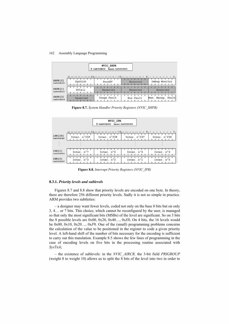
162 Assembly Language Programming
Figure 8.7. System Handler Priority Registers (NVIC_SHPR)
Figure 8.8. Interrupt Priority Registers (NVIC_IPR)
8.3.1. Priority levels and sublevels
Figures 8.7 and 8.8 show that priority levels are encoded on one byte. In theory,there are therefore 256 different priority levels. Sadly it is not so simple in practice.ARM provides two subtleties:
– a designer may want fewer levels, coded not only on the base 8 bits but on only3, 4… or 7 bits. This choice, which cannot be reconfigured by the user, is managedso that only the most significant bits (MSBs) of the level are significant. So on 3 bitsthe 8 possible levels are 0x00, 0x20, 0x40…, 0xE0. On 4 bits, the 16 levels wouldbe 0x00, 0x10, 0x20…, 0xF0. One of the (small) programming problems concernsthe calculation of the value to be positioned in the register to code a given prioritylevel. A left-hand shift of the number of bits necessary for the encoding is sufficientto carry out this translation. Example 8.5 shows the few lines of programming in thecase of encoding levels on five bits in the processing routine associated withSysTick;
– the existence of sublevels: in the NVIC_AIRCR, the 3-bit field PRIGROUP(weight 8 to weight 10) allows us to split the 8 bits of the level into two in order to
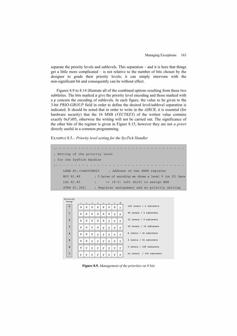
Managing Exceptions 163
separate the priority levels and sublevels. This separation – and it is here that thingsget a little more complicated – is not relative to the number of bits chosen by thedesigner to grade their priority levels; it can simply intervene with thenon-significant bit and consequently can be without effect.
Figures 8.9 to 8.14 illustrate all of the combined options resulting from these twosubtleties. The bits marked x give the priority level encoding and those marked witha y concern the encoding of sublevels. In each figure, the value to be given to the3-bit PRIO-GROUP field in order to define the desired level/sublevel separation isindicated. It should be noted that in order to write in the AIRCR, it is essential (forhardware security) that the 16 MSB (VECTKEY) of the written value containsexactly 0xFA05, otherwise the writing will not be carried out. The significance ofthe other bits of the register is given in Figure 8.15, however they are not a prioridirectly useful in a common programming.
EXAMPLE 8.5.– Priority level setting for the SysTick Handler
;– – – – – – – – – – – – – – – – – – – – – – – – – – – – – – – – – –
; Setting of the priority level
; for the SysTick Handler
;– – – – – – – – – – – – – – – – – – – – – – – – – – – – – – – – – –
LDRB R0,=0xE000ED23 ; Address of the SHPR register
MOV R1,#9 ; 5 bytes of encoding we chose a level 9 (on 32) here
LSL R1,#3 ; => (8-5) left shift to assign MSB
STRB R1,[R0] ; Register assignment and so priority setting
Figure 8.9. Management of the priorities on 8 bits
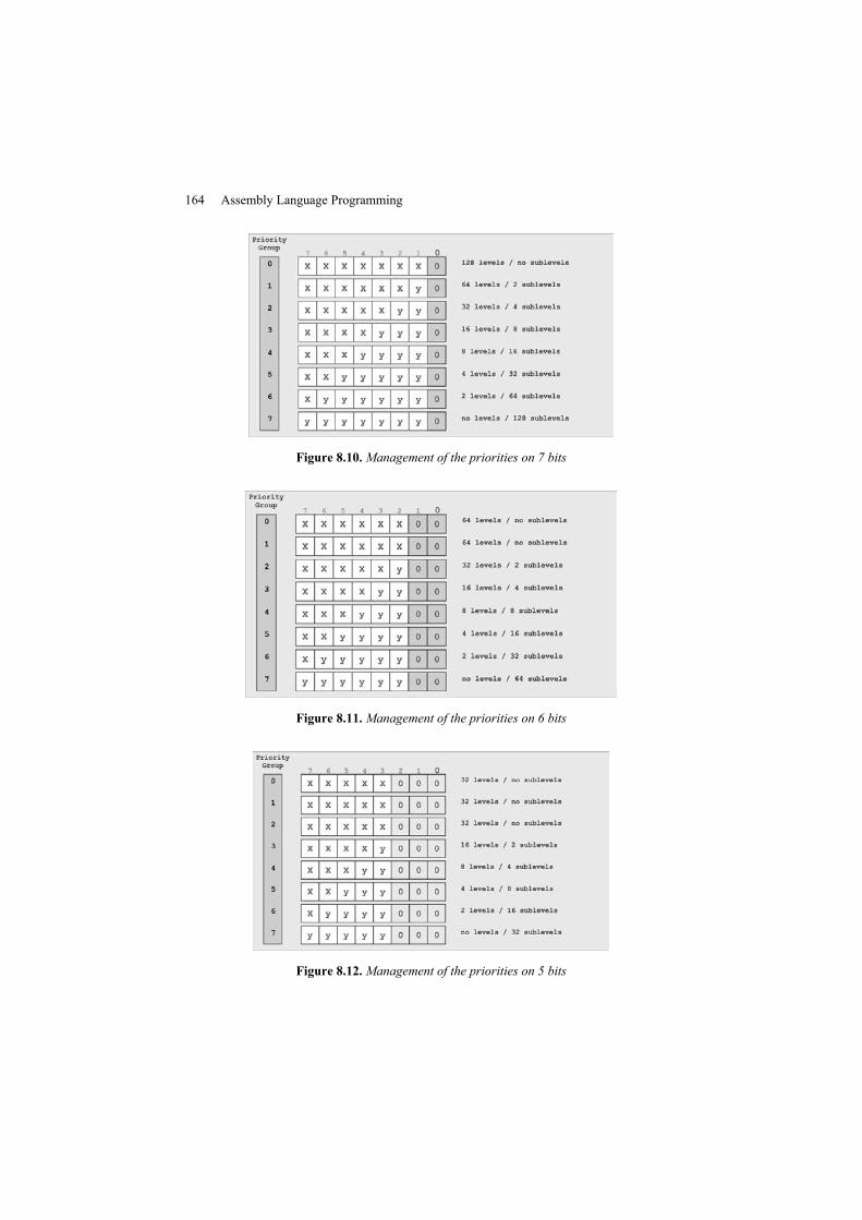
164 Assembly Language Programming
Figure 8.10. Management of the priorities on 7 bits
Figure 8.11. Management of the priorities on 6 bits
Figure 8.12. Management of the priorities on 5 bits
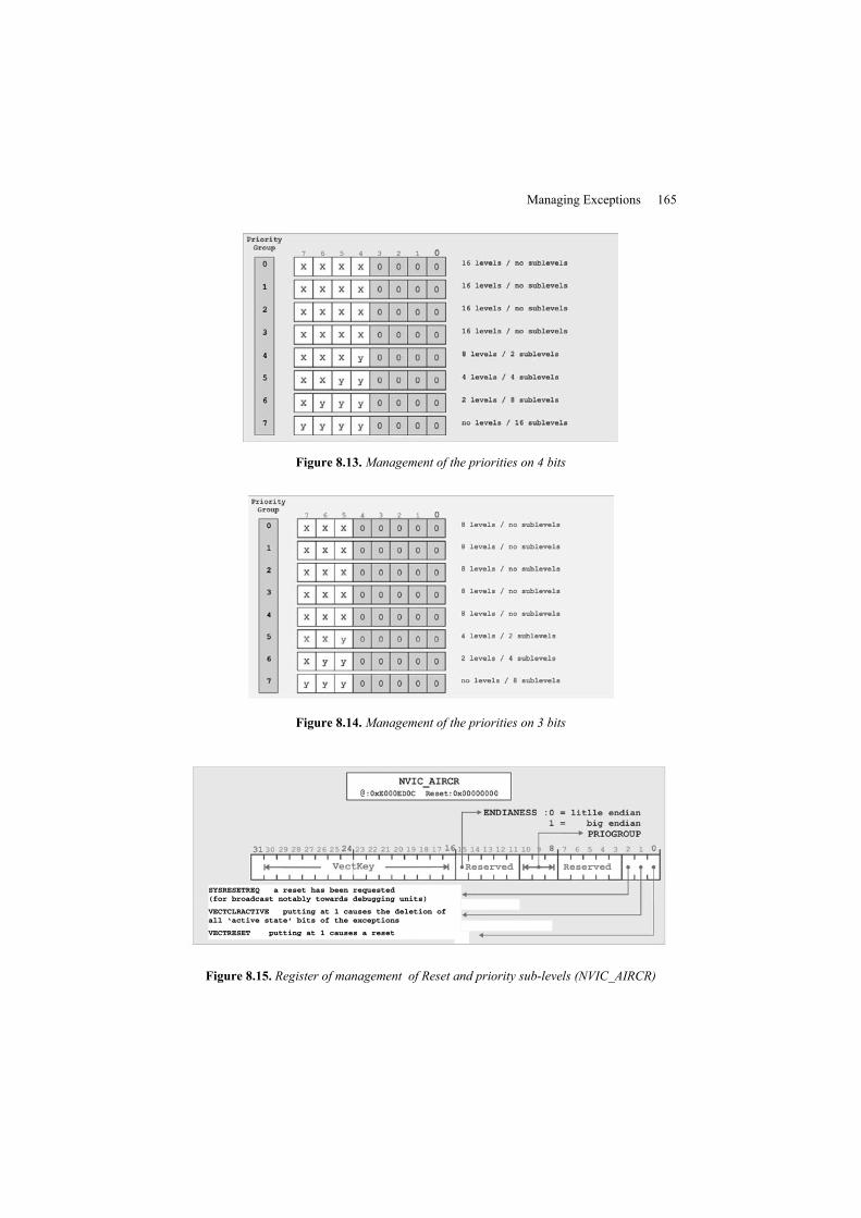
Managing Exceptions 165
Figure 8.13. Management of the priorities on 4 bits
Figure 8.14. Management of the priorities on 3 bits
SYSRESETREQ a reset has been requested(for broadcast notably towards debugging units)
VECTCLRACTIVE putting at 1 causes the deletion ofall ‘active state’ bits of the exceptions
VECTRESET putting at 1 causes a reset
Reserved Reserved
Figure 8.15. Register of management of Reset and priority sub-levels (NVIC_AIRCR)
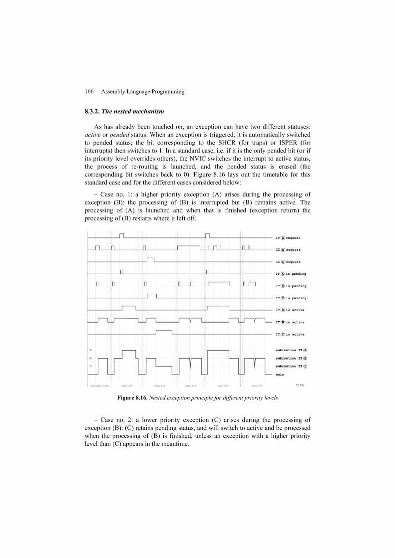
166 Assembly Language Programming
8.3.2. The nested mechanism
As has already been touched on, an exception can have two different statuses:active or pended status. When an exception is triggered, it is automatically switchedto pended status; the bit corresponding to the SHCR (for traps) or ISPER (forinterrupts) then switches to 1. In a standard case, i.e. if it is the only pended bit (or ifits priority level overrides others), the NVIC switches the interrupt to active status,the process of re-routing is launched, and the pended status is erased (thecorresponding bit switches back to 0). Figure 8.16 lays out the timetable for thisstandard case and for the different cases considered below:
– Case no. 1: a higher priority exception (A) arises during the processing ofexception (B): the processing of (B) is interrupted but (B) remains active. Theprocessing of (A) is launched and when that is finished (exception return) theprocessing of (B) restarts where it left off.
Figure 8.16. Nested exception principle for different priority levels
– Case no. 2: a lower priority exception (C) arises during the processing ofexception (B): (C) retains pending status, and will switch to active and be processedwhen the processing of (B) is finished, unless an exception with a higher prioritylevel than (C) appears in the meantime.
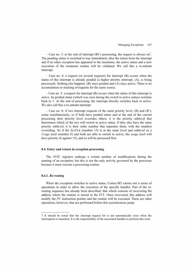
Managing Exceptions 167
– Case no. 3: at the end of interrupt (B)’s processing, the request is always on3.The pending status is switched to true immediately after the return from the interruptand if no other exception has appeared in the meantime, the active status and a newexecution of the treatment routine will be validated. We call this a re-entrantinterrupt.
– Case no. 4: a request (or several requests) for interrupt (B) occurs when thestatus of this interrupt is already pended (a higher priority interrupt, (A), is beingprocessed). Nothing else happens. (B) stays pended and (A) stays active. There is noaccumulation or stacking of requests for the same source.
– Case no. 5: a request for interrupt (B) occurs when the status of this interrupt isactive. Its pended status (which was reset during the switch to active status) switchesback to 1. At the end of processing, the interrupt directly switches back to active.We also call this a re-entrant interrupt.
– Case no. 6: if two interrupt requests of the same priority level, (B) and (B’),come simultaneously, or if both have pended status and at the end of the currentprocessing their priority level overrides others, it is the priority sublevel thatdetermines which of the two will switch to active status. If they also have the samepriority sublevel, it is their order number that separates them, with the smallestoverriding. So if the SysTick (number 15) is at the same level and sublevel as aUsage fault (number 6) and both are able to switch to active, the usage fault willhave priority (6 against 15), and so will be processed first.
8.4. Entry and return in exception processing
The NVIC registers undergo a certain number of modifications during therunning of an exception, but this is not the only activity governed by the processorbecause it must execute a processing routine.
8.4.1. Re-routing
When the exception switches to active status, Cortex-M3 carries out a series ofoperations in order to allow the execution of the specific handler. Part of the re-routing sequence has already been described: that which consists of recovering theaddress where the routine is stored in the IVT. Once recovered, this address willmodify the PC instruction pointer and the routine will be executed. There are otheroperations, however, that are performed before this asynchronous jump:
3 It should be noted that the interrupt request bit is not automatically reset when theinterruption is launched. It is the responsibility of the associated handler to perform this reset.

168 Assembly Language Programming
– eight registers are stored on the stack (MSP if the processor is in Handler modeand, in theory, PSP if it is in Thread mode: however, it is possible for Thread modeto use the MSP stack). These registers are, in order of stacking, PC, PSR, R0, R1,R2, R3, R12 and LR. The stack is originally in the state shown in Figure 8.17 whenstarting the processing routine;
– the processor, if it has not already, switches into Handler mode. The stackmust be MSP during exception processing;
– the LR is initialized with a return code (EXC_RETURN) that will allow it tocorrectly return from the exception. Indeed in this processor, in the opposite way tomany other types of architecture, there is no exception return instruction. This returnis triggered when the PC instruction pointer is loaded with a known value of returncode. This return code allows us to inform the processor of the mode in which itmust return (Thread or Handler) and so which system stack to use (MSP or PSP).The three unique values allowed are those in Table 8.1; any other code will cause ausage fault (the INVPC bit of UFSR being switched to 1).
Figure 8.17. State of the system stack after an exception re-routing
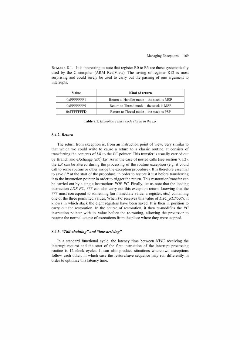
Managing Exceptions 169
REMARK 8.1.– It is interesting to note that register R0 to R3 are those systematicallyused by the C compiler (ARM RealView). The saving of register R12 is mostsurprising and could surely be used to carry out the passing of one argument tointerrupts.
Value Kind of return
0xFFFFFFF1 Return to Handler mode – the stack is MSP
0xFFFFFFF9 Return to Thread mode – the stack is MSP
0xFFFFFFFD Return to Thread mode – the stack is PSP
Table 8.1. Exception return code stored in the LR
8.4.2. Return
The return from exception is, from an instruction point of view, very similar tothat which we could write to cause a return to a classic routine. It consists oftransferring the contents of LR to the PC pointer. This transfer is usually carried outby Branch and eXchange (BX) LR. As in the case of nested calls (see section 7.1.2),the LR can be altered during the processing of the routine exception (e.g. it couldcall to some routine or other inside the exception procedure). It is therefore essentialto save LR at the start of the procedure, in order to restore it just before transferringit to the instruction pointer in order to trigger the return. This restoration/transfer canbe carried out by a single instruction: POP PC. Finally, let us note that the loadinginstruction LDR PC, ??? can also carry out this exception return, knowing that the??? must correspond to something (an immediate value, a register, etc.) containingone of the three permitted values. When PC receives this value of EXC_RETURN, itknows in which stack the eight registers have been saved. It is then in position tocarry out the restoration. In the course of restoration, it then re-modifies the PCinstruction pointer with its value before the re-routing, allowing the processor toresume the normal course of executions from the place where they were stopped.
8.4.3. “Tail-chaining” and “late-arriving”
In a standard functional cycle, the latency time between NVIC receiving theinterrupt request and the start of the first instruction of the interrupt processingroutine is 12 clock cycles. It can also produce situations where two exceptionsfollow each other, in which case the restore/save sequence may run differently inorder to optimize this latency time.
170 Assembly Language Programming
In the case of tail-chaining, as in case no. 3 (see Figure 8.16) it involves anexception (C) that must switch to active at the end of the previous exception (B). Inthis case it is pointless to perform the restoration at the end of (B) and to thenimmediately perform the save in order to launch (C), since there was no registermodification between the two points. This double sequence is therefore skipped. Atthe return time of (B), the processor switches directly to the processing of (C) andrestoration only takes place at the return of (C). In this case, the switch from (B) to(C) takes only 6 of the 12 cycles necessary without this “trick”.
The case of late-arriving involves a higher priority exception (A), which occurswhen the re-routing sequence of a lower level exception (B) has already started.This could correspond to case no. 1 by advancing the rising edge of the IT request(A) so that it takes place just after IT (B) switches to the active state. Here also thelatency time can be optimized by not performing a double save; i.e. by not launchinga save sequence after (A), since the save point is the same as (B). (A) will besubstituted for (B) in the re-routing and (B) will be switched to pended. At the endof (A), unless other higher priority exceptions have arisen, a tail-chainingmechanism will be implemented in order to resume the re-routing of (B).
8.4.4. Other useful registers for the NVIC
As we have seen in the course of this chapter, the NVIC module is the trueconductor for the organization of an exception handler into a hierarchy. To completeour account of its potential, there are some registers left to explain.
BasePri, PriMask and FaultMask are three core registers; therefore they do notoccupy a memory address. They are not part of the NVIC, but their role isnevertheless directly linked to exception management. They are described as specialin the documentation because they are not directly accessible. In order to accessthem, the code must use the special instructions MRS (Move from Register toSpecial) for reading and MSR (Move to Special Register) for writing, see Chapter 5.These two instructions require privileges in order to be executed.
The registers PriMask and FaultMask each have only one significant bit at 0.Thus when reading, the 31 MSB are always at 0 and, symmetrically, writing to thesebits will have no effect. These two registers, as their name suggests, allow us tomask exceptions. When the LSB is at 1 in FaultMask, no exceptions, apart from theNMI exception, will switch to active state and, if a request intervenes, will stay inpended state. As soon as the bit is reset, pended exceptions will switch to an activestate following the order of their respective priority. PriMask is identical toFaultMask, with the difference that in addition to NMI it also allows the launchingof the third exception with a non-configurable priority level, namely a hard fault.
Managing Exceptions 171
Prohibiting all (or nearly all) possible exceptions can be useful in “catastrophic”situations for which a real-time kernel will switch the processor to a “quasi-degraded” mode to hopefully provide solutions to these situations.
BasePri is similar. This involves a register of which the eight LSBs can besignificant. In effect, they contain a mask at the minimal priority level of exceptionsthat could switch to active state. All exceptions with a lower priority level wouldremain pended. Setting this register to 0x00 is equivalent to the absence of the mask.Two small pitfalls should be avoided for adjusting BasePri. First, it must beremembered that the priority scale is the reverse of normal numbering (level 3 islower than level 2). Then, as could be done for adjusting priorities in associatedregisters (see Example 8.5), we must not forget to carry out the 8 – n shifts on theleft of the desired value if the processor only codes priority levels on n bits.
The NVIC_STIR (Software Trigger Interrupt Register) is the last register ofNVIC that we will consider here. This register (@ 0xE000EF00) is an alternative tousing the NVIC_ISPER register, since in writing a value in the LSB (INTID) thisamounts to switching interrupt INTID into pending status. In an application toemulate the triggering of an interrupt with software, this second route willundoubtedly be faster and more practical to implement.

Chapter 9
From Listing to Executable:External Modularity
In the context of native development, the computer system on which an appliedproject is developed is exactly the same as the one that will execute the project.When we write a program for a μcontroller, this is never the case: indeed, there is noprogram under Cortex-M3 that allows us to develop another executive forCortex-M3. The programmer is in a cross-development situation where the writingand generation of an executable is done on a host computer system and theexecution is transported to the given target hardware. There may be a subtlety in thisbasic schema, however, which is the use of an emulator that allows us to develop aproject without a real target. This emulator is a program that works on the hostsystem and simulates the functioning of the μcontroller cycle-by-cycle, instructionby instruction. Although there are excellent emulators that are able to veryaccurately replicate the internal functioning of a processor, it is not unusual to finddifferences when executing on a real processor and the final validation phase cannotbe carried out without testing on a real target.
In the course of the cross-development phase, between writing the code in one(or several) “listing” file(s) and the execution of this code on a given processor,there are different stages (and therefore different tools), each of which is necessaryfor the proper realization of the whole. These are:
– the assembler, which interprets a source listing to create an object file;
– the linker, which puts together the different objects of the project and parts ofthe library to make the executable file;
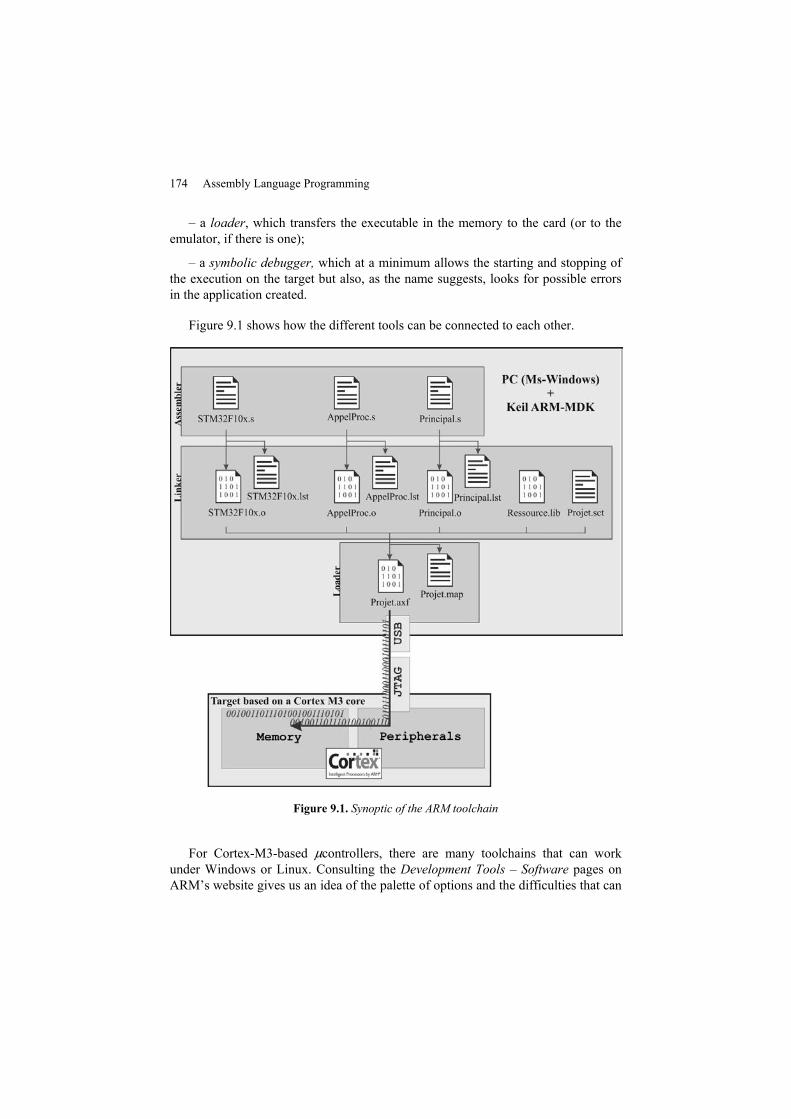
174 Assembly Language Programming
– a loader, which transfers the executable in the memory to the card (or to theemulator, if there is one);
– a symbolic debugger, which at a minimum allows the starting and stopping ofthe execution on the target but also, as the name suggests, looks for possible errorsin the application created.
Figure 9.1 shows how the different tools can be connected to each other.
Figure 9.1. Synoptic of the ARM toolchain
For Cortex-M3-based μcontrollers, there are many toolchains that can workunder Windows or Linux. Consulting the Development Tools – Software pages onARM’s website gives us an idea of the palette of options and the difficulties that can
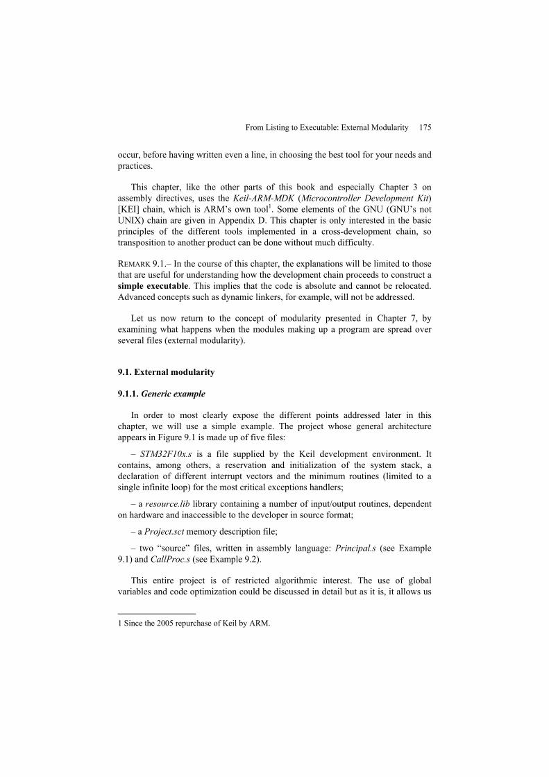
From Listing to Executable: External Modularity 175
occur, before having written even a line, in choosing the best tool for your needs andpractices.
This chapter, like the other parts of this book and especially Chapter 3 onassembly directives, uses the Keil-ARM-MDK (Microcontroller Development Kit)[KEI] chain, which is ARM’s own tool1. Some elements of the GNU (GNU’s notUNIX) chain are given in Appendix D. This chapter is only interested in the basicprinciples of the different tools implemented in a cross-development chain, sotransposition to another product can be done without much difficulty.
REMARK 9.1.– In the course of this chapter, the explanations will be limited to thosethat are useful for understanding how the development chain proceeds to construct asimple executable. This implies that the code is absolute and cannot be relocated.Advanced concepts such as dynamic linkers, for example, will not be addressed.
Let us now return to the concept of modularity presented in Chapter 7, byexamining what happens when the modules making up a program are spread overseveral files (external modularity).
9.1. External modularity
9.1.1. Generic example
In order to most clearly expose the different points addressed later in thischapter, we will use a simple example. The project whose general architectureappears in Figure 9.1 is made up of five files:
– STM32F10x.s is a file supplied by the Keil development environment. Itcontains, among others, a reservation and initialization of the system stack, adeclaration of different interrupt vectors and the minimum routines (limited to asingle infinite loop) for the most critical exceptions handlers;
– a resource.lib library containing a number of input/output routines, dependenton hardware and inaccessible to the developer in source format;
– a Project.sct memory description file;
– two “source” files, written in assembly language: Principal.s (see Example9.1) and CallProc.s (see Example 9.2).
This entire project is of restricted algorithmic interest. The use of globalvariables and code optimization could be discussed in detail but as it is, it allows us
1 Since the 2005 repurchase of Keil by ARM.
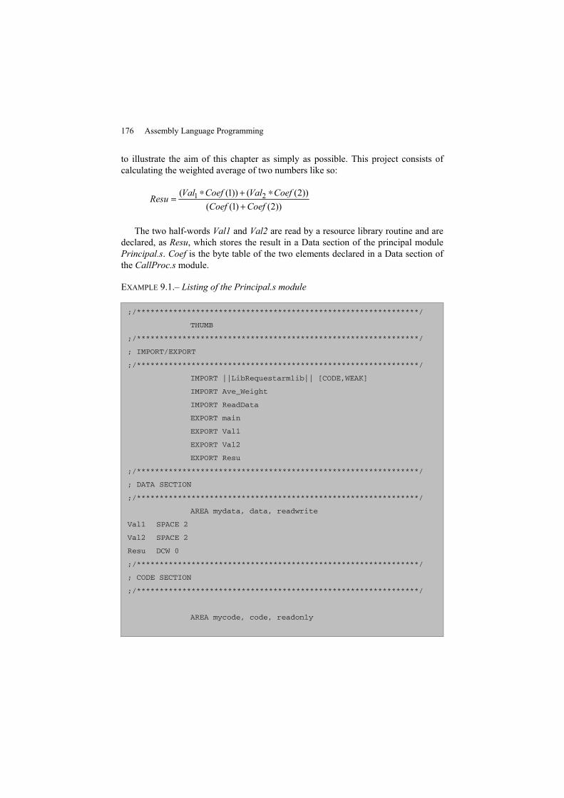
176 Assembly Language Programming
to illustrate the aim of this chapter as simply as possible. This project consists ofcalculating the weighted average of two numbers like so:
1 2( (1)) ( (2))( (1) (2))
Val Coef Val CoefResuCoef Coef
∗ + ∗=
+
The two half-words Val1 and Val2 are read by a resource library routine and aredeclared, as Resu, which stores the result in a Data section of the principal modulePrincipal.s. Coef is the byte table of the two elements declared in a Data section ofthe CallProc.s module.
EXAMPLE 9.1.– Listing of the Principal.s module
;/**************************************************************/
THUMB
;/**************************************************************/
; IMPORT/EXPORT
;/**************************************************************/
IMPORT ||LibRequestarmlib|| [CODE,WEAK]
IMPORT Ave_Weight
IMPORT ReadData
EXPORT main
EXPORT Val1
EXPORT Val2
EXPORT Resu
;/**************************************************************/
; DATA SECTION
;/**************************************************************/
AREA mydata, data, readwrite
Val1 SPACE 2
Val2 SPACE 2
Resu DCW 0
;/**************************************************************/
; CODE SECTION
;/**************************************************************/
AREA mycode, code, readonly
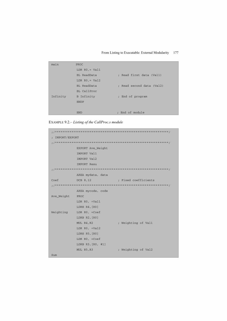
From Listing to Executable: External Modularity 177
main PROC
LDR R0,= Val1
BL ReadData ; Read first data (Val1)
LDR R0,= Val2
BL ReadData ; Read second data (Val2)
BL CallProc
Infinity B Infinity ; End of program
ENDP
END ; End of module
EXAMPLE 9.2.– Listing of the CallProc.s module
;/**************************************************************/
; IMPORT/EXPORT
;/**************************************************************/
EXPORT Ave_Weight
IMPORT Val1
IMPORT Val2
IMPORT Resu
;/**************************************************************/
AREA mydata, data
Coef DCB 8,12 ; Fixed coefficients
;/**************************************************************/
AREA mycode, code
Ave_Weight PROC
LDR R0, =Val1
LDRH R4,[R0]
Weighting LDR R0, =Coef
LDRB R2,[R0]
MUL R4,R2 ; Weighting of Val1
LDR R0, =Val2
LDRH R5,[R0]
LDR R0, =Coef
LDRB R3,[R0, #1]
MUL R5,R3 ; Weighting of Val2
Sum
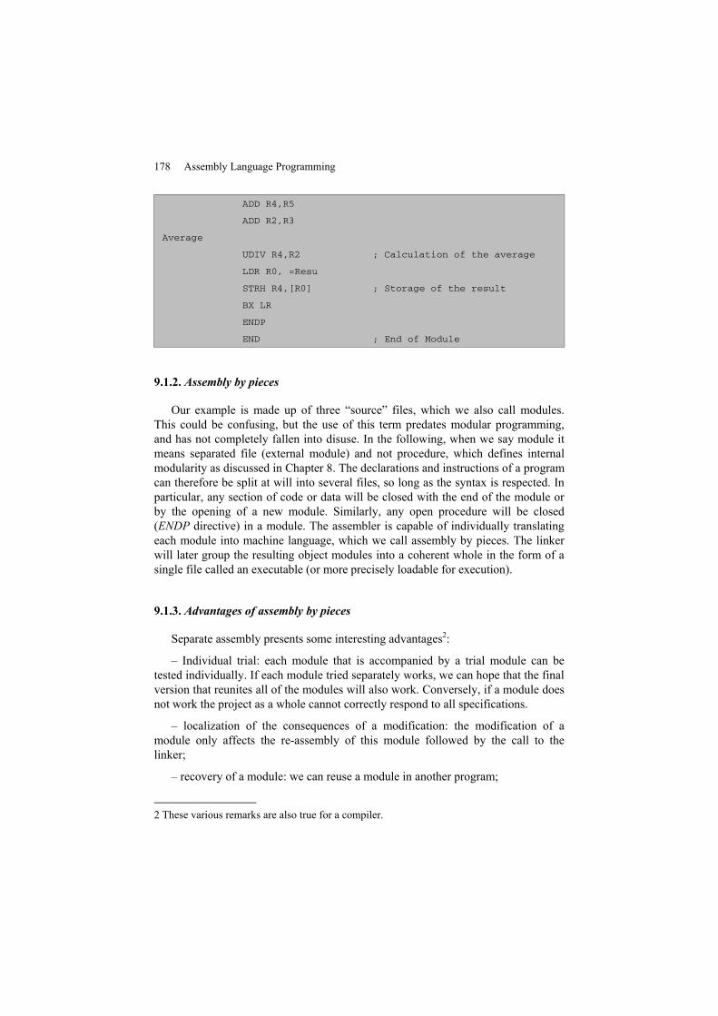
178 Assembly Language Programming
ADD R4,R5
ADD R2,R3
Average
UDIV R4,R2 ; Calculation of the average
LDR R0, =Resu
STRH R4,[R0] ; Storage of the result
BX LR
ENDP
END ; End of Module
9.1.2. Assembly by pieces
Our example is made up of three “source” files, which we also call modules.This could be confusing, but the use of this term predates modular programming,and has not completely fallen into disuse. In the following, when we say module itmeans separated file (external module) and not procedure, which defines internalmodularity as discussed in Chapter 8. The declarations and instructions of a programcan therefore be split at will into several files, so long as the syntax is respected. Inparticular, any section of code or data will be closed with the end of the module orby the opening of a new module. Similarly, any open procedure will be closed(ENDP directive) in a module. The assembler is capable of individually translatingeach module into machine language, which we call assembly by pieces. The linkerwill later group the resulting object modules into a coherent whole in the form of asingle file called an executable (or more precisely loadable for execution).
9.1.3. Advantages of assembly by pieces
Separate assembly presents some interesting advantages2:
– Individual trial: each module that is accompanied by a trial module can betested individually. If each module tried separately works, we can hope that the finalversion that reunites all of the modules will also work. Conversely, if a module doesnot work the project as a whole cannot correctly respond to all specifications.
– localization of the consequences of a modification: the modification of amodule only affects the re-assembly of this module followed by the call to thelinker;
– recovery of a module: we can reuse a module in another program;
2 These various remarks are also true for a compiler.
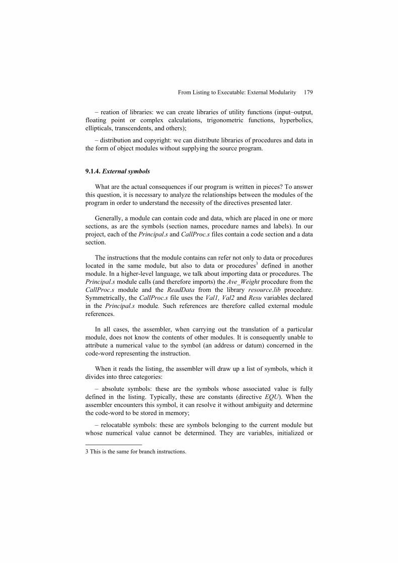
From Listing to Executable: External Modularity 179
– reation of libraries: we can create libraries of utility functions (input–output,floating point or complex calculations, trigonometric functions, hyperbolics,ellipticals, transcendents, and others);
– distribution and copyright: we can distribute libraries of procedures and data inthe form of object modules without supplying the source program.
9.1.4. External symbols
What are the actual consequences if our program is written in pieces? To answerthis question, it is necessary to analyze the relationships between the modules of theprogram in order to understand the necessity of the directives presented later.
Generally, a module can contain code and data, which are placed in one or moresections, as are the symbols (section names, procedure names and labels). In ourproject, each of the Principal.s and CallProc.s files contain a code section and a datasection.
The instructions that the module contains can refer not only to data or procedureslocated in the same module, but also to data or procedures3 defined in anothermodule. In a higher-level language, we talk about importing data or procedures. ThePrincipal.s module calls (and therefore imports) the Ave_Weight procedure from theCallProc.s module and the ReadData from the library resource.lib procedure.Symmetrically, the CallProc.s file uses the Val1, Val2 and Resu variables declaredin the Principal.s module. Such references are therefore called external modulereferences.
In all cases, the assembler, when carrying out the translation of a particularmodule, does not know the contents of other modules. It is consequently unable toattribute a numerical value to the symbol (an address or datum) concerned in thecode-word representing the instruction.
When it reads the listing, the assembler will draw up a list of symbols, which itdivides into three categories:
– absolute symbols: these are the symbols whose associated value is fullydefined in the listing. Typically, these are constants (directive EQU). When theassembler encounters this symbol, it can resolve it without ambiguity and determinethe code-word to be stored in memory;
– relocatable symbols: these are symbols belonging to the current module butwhose numerical value cannot be determined. They are variables, initialized or
3 This is the same for branch instructions.
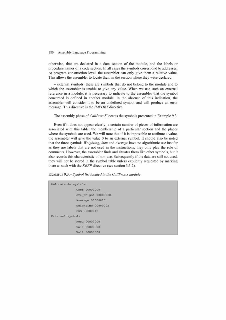
180 Assembly Language Programming
otherwise, that are declared in a data section of the module, and the labels orprocedure names of a code section. In all cases the symbols correspond to addresses.At program construction level, the assembler can only give them a relative value.This allows the assembler to locate them in the section where they were declared;
– external symbols: these are symbols that do not belong to the module and towhich the assembler is unable to give any value. When we use such an externalreference in a module, it is necessary to indicate to the assembler that the symbolconcerned is defined in another module. In the absence of this indication, theassembler will consider it to be an undefined symbol and will produce an errormessage. This directive is the IMPORT directive.
The assembly phase of CallProc.S locates the symbols presented in Example 9.3.
Even if it does not appear clearly, a certain number of pieces of information areassociated with this table: the membership of a particular section and the placeswhere the symbols are used. We will note that if it is impossible to attribute a value,the assembler will give the value 0 to an external symbol. It should also be notedthat the three symbols Weighting, Sum and Average have no algorithmic use insofaras they are labels that are not used in the instructions; they only play the role ofcomments. However, the assembler finds and situates them like other symbols, but italso records this characteristic of non-use. Subsequently if the data are still not used,they will not be stored in the symbol table unless explicitly requested by markingthem as such with the KEEP directive (see section 3.5.2).
EXAMPLE 9.3.– Symbol list located in the CallProc.s module
Relocatable symbols
Coef 00000000
Ave_Weight 00000000
Average 0000001C
Weighting 0000000E
Sum 00000018
External symbols
Resu 00000000
Val1 00000000
Val2 00000000
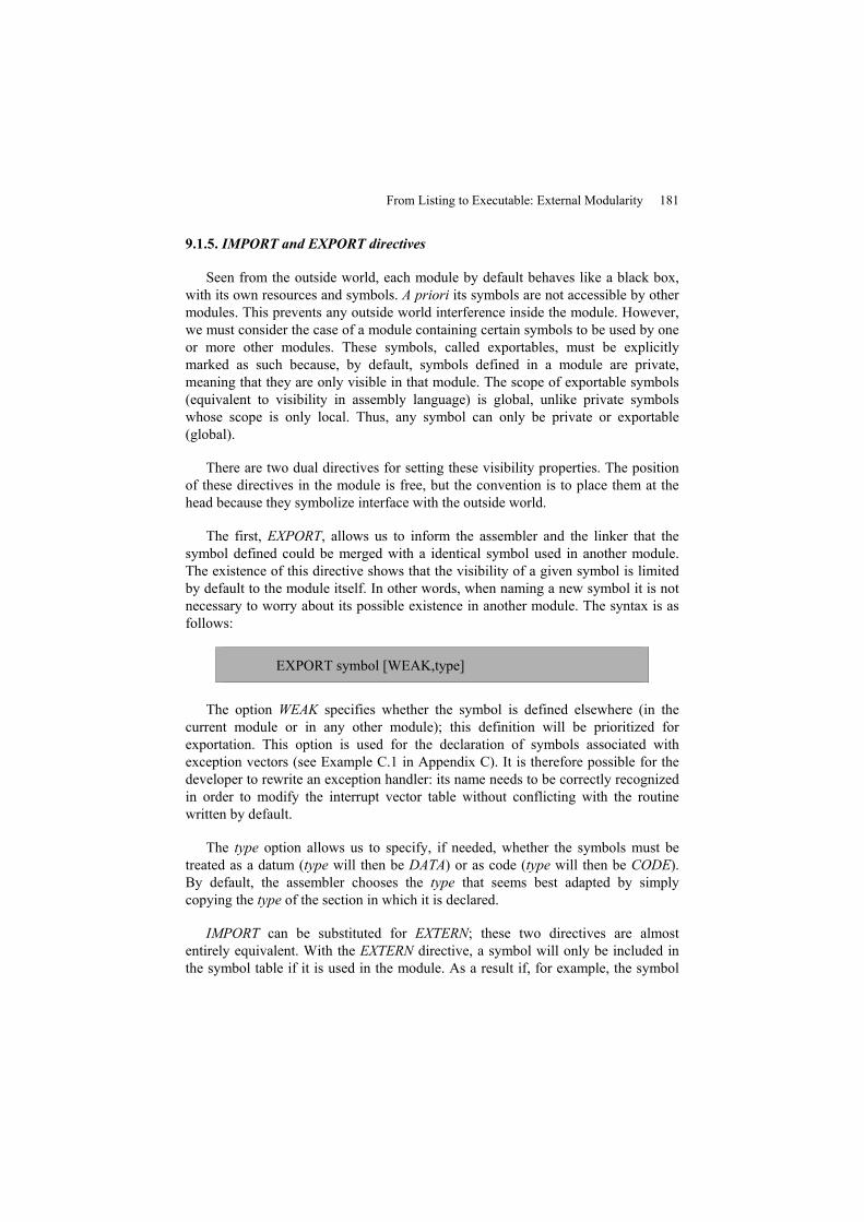
From Listing to Executable: External Modularity 181
9.1.5. IMPORT and EXPORT directives
Seen from the outside world, each module by default behaves like a black box,with its own resources and symbols. A priori its symbols are not accessible by othermodules. This prevents any outside world interference inside the module. However,we must consider the case of a module containing certain symbols to be used by oneor more other modules. These symbols, called exportables, must be explicitlymarked as such because, by default, symbols defined in a module are private,meaning that they are only visible in that module. The scope of exportable symbols(equivalent to visibility in assembly language) is global, unlike private symbolswhose scope is only local. Thus, any symbol can only be private or exportable(global).
There are two dual directives for setting these visibility properties. The positionof these directives in the module is free, but the convention is to place them at thehead because they symbolize interface with the outside world.
The first, EXPORT, allows us to inform the assembler and the linker that thesymbol defined could be merged with a identical symbol used in another module.The existence of this directive shows that the visibility of a given symbol is limitedby default to the module itself. In other words, when naming a new symbol it is notnecessary to worry about its possible existence in another module. The syntax is asfollows:
EXPORT symbol [WEAK,type]
The option WEAK specifies whether the symbol is defined elsewhere (in thecurrent module or in any other module); this definition will be prioritized forexportation. This option is used for the declaration of symbols associated withexception vectors (see Example C.1 in Appendix C). It is therefore possible for thedeveloper to rewrite an exception handler: its name needs to be correctly recognizedin order to modify the interrupt vector table without conflicting with the routinewritten by default.
The type option allows us to specify, if needed, whether the symbols must betreated as a datum (type will then be DATA) or as code (type will then be CODE).By default, the assembler chooses the type that seems best adapted by simplycopying the type of the section in which it is declared.
IMPORT can be substituted for EXTERN; these two directives are almostentirely equivalent. With the EXTERN directive, a symbol will only be included inthe symbol table if it is used in the module. As a result if, for example, the symbol
182 Assembly Language Programming
VarForgot is declared in a project and is not used in the code of the current module,the directive IMPORT VarForgot will generate a linker error, since it will be still beincluded in the list and is consequently searched for by the linker. Conversely,directive EXTERNE VarForgot will do nothing and the linker will therefore notworry about not finding it.
The IMPORT directive performs the opposite function of the preceding directive:it enables the assembler to know whether such a qualified symbol comes from anexternal module. If this is the case, it can accept the symbol’s use in the module’scode.
IMPORT symbol [WEAK,type]
The type option has the same meaning as it does in the EXPORT directive.
In the absence of the WEAK option on a symbol, if the linker cannot recognizethe symbol (i.e. if the symbol does not exist elsewhere in the project), it will cause afatal error in the construction of the project. Conversely, if the symbol is marked asWEAK during its importation, the linker will always be able to resolve the symbolby giving it a default value, if any. If the symbol is a destination (B symbol, forexample) its default value will be the address of the next instruction. The jump willthen be equivalent to NOP (No Operation). In other cases, the default value will be0. Poorly controlled use of WEAK in the importations of a variable can bedangerous.
As an example, let us imagine forgetting the exportations of Resu in thePrincipal.s file and the confirmation of this same symbol by WEAK in CallProc.s.This would result in a project that was correctly constructed, but the result would bestored at the memory address 0x0000000! We must then hope that a Reset will notoccur afterwards, since the stack address would no longer be valid (see section 8.1).Like the EXTERN directive for IMPORT, the EXPORT directive can be substituted(with no subtlety of use in this case) by the GLOBAL directive.
9.2. The role of the assembler
The principal role of the assembler is to translate the contents of the sourcemodule written in assembly language into machine language code-words (which weshould remember are coded on 16 or 32 bits). It is not capable of carrying out acomplete work, however, because it lacks a series of data: it does not know the valueof external symbols, nor the address where each section defined in the source will beplaced. Nevertheless, it is capable of carrying out its job. We will see how it
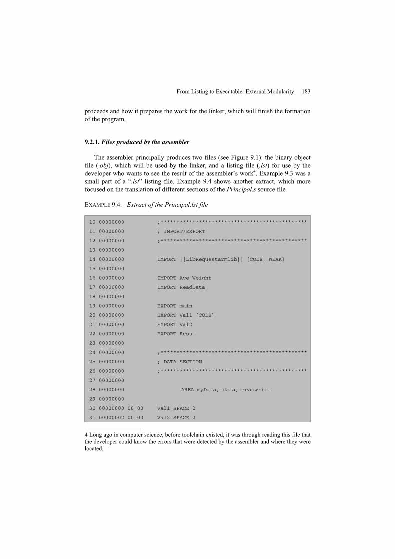
From Listing to Executable: External Modularity 183
proceeds and how it prepares the work for the linker, which will finish the formationof the program.
9.2.1. Files produced by the assembler
The assembler principally produces two files (see Figure 9.1): the binary objectfile (.obj), which will be used by the linker, and a listing file (.lst) for use by thedeveloper who wants to see the result of the assembler’s work4. Example 9.3 was asmall part of a “.lst” listing file. Example 9.4 shows another extract, which morefocused on the translation of different sections of the Principal.s source file.
EXAMPLE 9.4.– Extract of the Principal.lst file
10 00000000 ;**********************************************
11 00000000 ; IMPORT/EXPORT
12 00000000 ;**********************************************
13 00000000
14 00000000 IMPORT ||LibRequestarmlib|| [CODE, WEAK]
15 00000000
16 00000000 IMPORT Ave_Weight
17 00000000 IMPORT ReadData
18 00000000
19 00000000 EXPORT main
20 00000000 EXPORT Val1 [CODE]
21 00000000 EXPORT Val2
22 00000000 EXPORT Resu
23 00000000
24 00000000 ;**********************************************
25 00000000 ; DATA SECTION
26 00000000 ;**********************************************
27 00000000
28 00000000 AREA myData, data, readwrite
29 00000000
30 00000000 00 00 Val1 SPACE 2
31 00000002 00 00 Val2 SPACE 2
4 Long ago in computer science, before toolchain existed, it was through reading this file thatthe developer could know the errors that were detected by the assembler and where they werelocated.
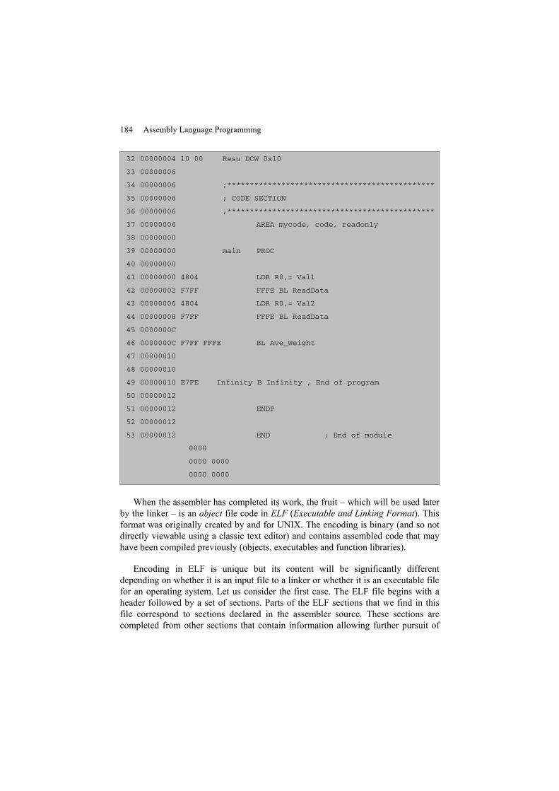
184 Assembly Language Programming
32 00000004 10 00 Resu DCW 0x10
33 00000006
34 00000006 ;**********************************************
35 00000006 ; CODE SECTION
36 00000006 ;**********************************************
37 00000006 AREA mycode, code, readonly
38 00000000
39 00000000 main PROC
40 00000000
41 00000000 4804 LDR R0,= Val1
42 00000002 F7FF FFFE BL ReadData
43 00000006 4804 LDR R0,= Val2
44 00000008 F7FF FFFE BL ReadData
45 0000000C
46 0000000C F7FF FFFE BL Ave_Weight
47 00000010
48 00000010
49 00000010 E7FE Infinity B Infinity ; End of program
50 00000012
51 00000012 ENDP
52 00000012
53 00000012 END ; End of module
0000
0000 0000
0000 0000
When the assembler has completed its work, the fruit – which will be used laterby the linker – is an object file code in ELF (Executable and Linking Format). Thisformat was originally created by and for UNIX. The encoding is binary (and so notdirectly viewable using a classic text editor) and contains assembled code that mayhave been compiled previously (objects, executables and function libraries).
Encoding in ELF is unique but its content will be significantly differentdepending on whether it is an input file to a linker or whether it is an executable filefor an operating system. Let us consider the first case. The ELF file begins with aheader followed by a set of sections. Parts of the ELF sections that we find in thisfile correspond to sections declared in the assembler source. These sections arecompleted from other sections that contain information allowing further pursuit of
From Listing to Executable: External Modularity 185
the construction of the executable image of the project. We can cite containing thesymbol table (see section 9.2.3) or those dedicated to relocation tables (seesection 9.4) as examples of sections. Finally, other sections are optional, such asthose that group the necessary data for the functioning of a debugger (see section9.4).
REMARK 9.2.– There are specific programs for reading files coded in ELF in orderto retrieve and view information related to its content. In the ARM developmentchain, this tool corresponds to the executable FROMELF program.
9.2.2. Placement counters
The assembler carries out all of its work in a relative manner. For each module itnumbers each line, as you can see in the first column of Example 9.4. This firstsearch is not very complicated, since it just consists of locating the ASCII charactercarriage return in the processed listing. It should be noted, however, that emptylines are also located, an important detail for a development system that mustindicate the line where an error is located or for development when the listing is putin parallel with disassembled code. For each section – whether it is code or data –the assembler also uses a placement counter (the second column of the lst file)whose initial value is 00000000. The departure address of each section is thereforeprovisionally set at 0. In the case of a code section, insofar as it carries out itstranslation, the assembler increases the value of the placement counter by 2 or 4,depending on the size of the instruction. The placement counter therefore indicatesthe relative position of each instruction. It works in the same way for each datasection, the incrementation of its internal counter depending on the size of thevariable.
For each new section, the placement counter restarts at 000000. If a section isclosed but opens a second time in the same source file, the placement counter is notreset to 0 but continues from the last previous value, which de facto means theconcatenation of two half sections.
9.2.3. First pass: symbol table
Classically an assembler works in two passes. In the first pass, it scans all of thetext to raise all of the symbols and establish a symbol table. We have already shownhow this table was presented in Example 9.3, however there is another importantelement to be added: the Literal Pool zones. In fact, when an assembler scans all ofthe instructions making up the code, it locates the addresses (always in a relativemanner) of the section being analyzed where it will be possible to store the
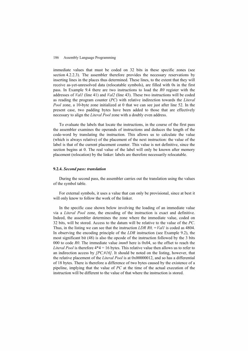
186 Assembly Language Programming
immediate values that must be coded on 32 bits in these specific zones (seesection 4.2.2.3). The assembler therefore provides the necessary reservations byinserting lines in the places thus determined. These lines, to the extent that they willreceive as-yet-unresolved data (relocatable symbols), are filled with 0s in the firstpass. In Example 9.4 there are two instructions to load the R0 register with theaddresses of Val1 (line 41) and Val2 (line 43). These two instructions will be codedas reading the program counter (PC) with relative indirection towards the LiteralPool zone, a 10-byte zone initialized at 0 that we can see just after line 52. In thepresent case, two padding bytes have been added to those that are effectivelynecessary to align the Literal Pool zone with a doubly even address.
To evaluate the labels that locate the instructions, in the course of the first passthe assembler examines the operands of instructions and deduces the length of thecode-word by translating the instruction. This allows us to calculate the value(which is always relative) of the placement of the next instruction: the value of thelabel is that of the current placement counter. This value is not definitive, since thesection begins at 0. The real value of the label will only be known after memoryplacement (relocation) by the linker: labels are therefore necessarily relocatable.
9.2.4. Second pass: translation
During the second pass, the assembler carries out the translation using the valuesof the symbol table.
For external symbols, it uses a value that can only be provisional, since at best itwill only know to follow the work of the linker.
In the specific case shown below involving the loading of an immediate valuevia a Literal Pool zone, the encoding of the instruction is exact and definitive.Indeed, the assembler determines the zone where the immediate value, coded on32 bits, will be stored. Access to the datum will be relative to the value of the PC.Thus, in the listing we can see that the instruction LDR R0, =Val1 is coded as 4804.In observing the encoding principle of the LDR instruction (see Example 9.2), themost significant bit (48) is also the opcode of the instruction followed by the 3 bits000 to code R0. The immediate value imm8 here is 0x04, so the offset to reach theLiteral Pool is therefore 4*4 = 16 bytes. This relative value then allows us to refer toan indirection access by [PC,#16]. It should be noted on the listing, however, thatthe relative placement of the Literal Pool is at 0x00000012, and so has a differentialof 18 bytes. There is therefore a difference of two bytes caused by the existence of apipeline, implying that the value of PC at the time of the actual execution of theinstruction will be different to the value of that where the instruction is stored.

From Listing to Executable: External Modularity 187
For references to internal labels, the assembler uses the value of the label givenby its symbol table. In some cases, as in the case of jumps for example, encodingrelative to the operand is possible. Thus the translation is direct. For references toexternal labels, the encoding is never directly possible to the extent that the label isunresolved. The assembler will therefore introduce a partially false operand codethat will belong to the linker, in order to give the correct value. In our example, thejump to the ReadData (line 42) procedure is coded as 0xF7FFFFFE. The first sevenbits also correspond to the opcode of the BL (Branch with Link) instruction (11110)but the remaining 23 bits do not allow the decoding of a valid subroutine address inthis state. In this case we are dealing with a coded instruction that must be“relocated” by the linker.
Figure 9.2. Thumb encoding of an LDR instruction
9.2.5. Relocation table
Finally we obtain a partially erroneous code. It is erroneous in the sense that anyabsolute reference to a label or any use of external symbols leads to false code-words. As it will be corrected by the linker, it is necessary for the assembler toprovide the linker with useful information. The assembler communicates thisinformation with a relocation table where the list of instructions to be corrected isindicated, as are the rules to apply to make the corrections. We will not go into howthese relocation tables work, partly because complete information on theirfunctioning is unavailable but partly because the developer does not have directaccess and consequently it is impossible to modify its contents. It is still interesting,however, at least for curiosity’s sake, to look at the contents of one of these tables:Example 9.5 gives the third ELF section of the Principal.o file. This sectioncorresponds to the relocation table of the CODE section mycode of thecorresponding source file.
We can see that for this small section of code the linker will have fiverelocations to carry out. Each of these relocations is marked by its offset (secondcolumn). Relocation may come completely from outside (Ref indicated in the lastcolumn) or in a relative manner with respect to another section of the currentmodule (the name of the section where the relative datum will be situated appears inthe last column).
188 Assembly Language Programming
EXAMPLE 9.5.– Extract from an ELF file: the relocation table
** Section #3 ’.relmycode’ (SHT_REL)
Size : 40 bytes (alignment 4)
Symbol table #6 ’.symtab’
5 relocations applied to section #2 ’mycode’
# Offset Relocation Type Wrt Symbol Defined in
0 0x00000008 10 R_ARM_THM_CALL 12 ReadData Ref
1 0x00000008 10 R_ARM_THM_CALL 12 ReadData Ref
2 0x0000000C 10 R_ARM_THM_CALL 13 Ave_Weight Ref
3 0x00000014 2 R_ARM_ABS32 8 Val1 #1 ’mydata’
4 0x000000018 2 R_ARM_ABS32 9 Val2 #1 ’mydata’
9.3. The role of the linker
The linker completes the creation of a program by bringing together the variousmodules into a single file called an executable.
9.3.1. Functioning principle
When we call the linker (also called the link editor), we give it a list of modulesto bring together that contain each of a number of input sections. The linker is alsoinformed of the memory layout of the target on which the program will be executed.This layout is coded in the Project.sct file. The work to be done is relatively simple:the different input sections are grouped in order to give them addresses compatiblewith the memory layout.
In our example, by invalidating the options that allow the inclusion of debugginginformation, the CallProc.o file contains 16 different sections, and the Principal.ofile contains 11 of them. We then indicate that there is 128 KB of read-only memory(ROM) from address 0x08000000 and 20 KB of random access memory (RAM)from address 0x20000000.
REMARK 9.3.– The memory layout used here is that of a STM32103RB, which is theμcontroller of the target for this project. The absence of memory for the lowestaddresses should be noted, as this is contrary to the imposed localization of theinterrupt vector table (see Example 8.1). This contradiction is only apparent becauseSTMicro has chosen to insert an alias between the [0x00000000–0x07FFFFFF] zone
From Listing to Executable: External Modularity 189
and another zone as a function of the state of two pins after a reset. The principle ofthis maneuver is to be able to find the reset vector (and so the reset code) in internalFlash, in system memory or in internal static RAM. Here the target zone of the aliasis [0x08000000–0x10000000], which corresponds to the internal Flash memory. Inthis project, the lower addresses are present, even if they are virtual.
Let us remember that Cortex-M3 architecture is of the Harvard type, so there is acomplete separation of the code and data zones (see Figure 1.5). The linker musttherefore assign the code sections with addresses present in the [0x00000000–0x1FFFFFFF] zone and the data sections with addresses present in the[0x20000000–0x2FFFFFFF] zone.
Each input section received by the linker has a type and attributes. The threemain types are:
– a RO (Read Only) zone, which is a ROM or Flash zone whose typical contentis code. It is common (in the GNU world, for example) to see the abbreviation .textfor this type of section;
– a RW (Read/Write) zone, which is a RAM zone whose typical contents areinitialized data. The usual synonym for this is .data;
– a ZI (Zero Initialized) zone. This is also a read/write zone that will containuninitialized data. By default ZI zones are set to 0. This type of section is also called.bss.
In addition to this typing, there is a whole series of attributes which, in the caseof those found at the head of ELF files, allow the recording of different informationthat may be needed by the linker, loading or even symbolic debugging.
In a first simplistic (but not completely false) vision, the work of the linkertherefore consists of retrieving the list and the size of the set of code and datasections, bringing them together and distributing them in corresponding memoryzones. It concatenates the different pieces by properly merging the symbol tables: itis sufficient to correct the values of the labels of successively added modules byprogressively incrementing the size of the sections. Finally, the linker changes theinitial address of each section by determining its definitive address. Once more, itcarries out the correction of instructions using the relocation tables. This simplisticvision is not enough: in fact the product of the linker cannot properly be called anexecutable file. It produces an image of an executable that will be “seen” differentlyat the loading level or at the execution level itself.
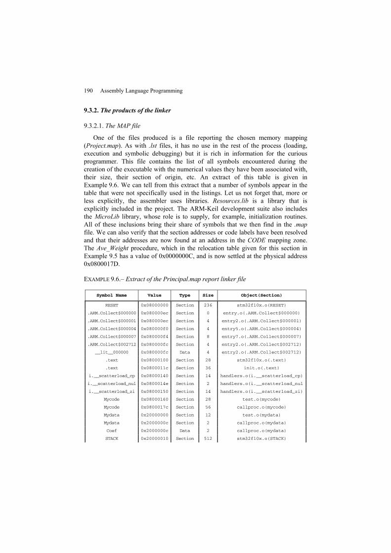
190 Assembly Language Programming
9.3.2. The products of the linker
9.3.2.1. The MAP file
One of the files produced is a file reporting the chosen memory mapping(Project.map). As with .lst files, it has no use in the rest of the process (loading,execution and symbolic debugging) but it is rich in information for the curiousprogrammer. This file contains the list of all symbols encountered during thecreation of the executable with the numerical values they have been associated with,their size, their section of origin, etc. An extract of this table is given inExample 9.6. We can tell from this extract that a number of symbols appear in thetable that were not specifically used in the listings. Let us not forget that, more orless explicitly, the assembler uses libraries. Resources.lib is a library that isexplicitly included in the project. The ARM-Keil development suite also includesthe MicroLib library, whose role is to supply, for example, initialization routines.All of these inclusions bring their share of symbols that we then find in the .mapfile. We can also verify that the section addresses or code labels have been resolvedand that their addresses are now found at an address in the CODE mapping zone.The Ave_Weight procedure, which in the relocation table given for this section inExample 9.5 has a value of 0x0000000C, and is now settled at the physical address0x0800017D.
EXAMPLE 9.6.– Extract of the Principal.map report linker file
Symbol Name Value Type Size Object(Section)
RESET 0x08000000 Section 236 stm32f10x.o(RESET)
.ARM.Collect$000000 0x080000ec Section 0 entry.o(.ARM.Collect$000000)
.ARM.Collect$000001 0x080000ec Section 4 entry2.o(.ARM.Collect$000001)
.ARM.Collect$000004 0x080000f0 Section 4 entry5.o(.ARM.Collect$000004)
.ARM.Collect$000007 0x080000f4 Section 8 entry7.o(.ARM.Collect$000007)
.ARM.Collect$002712 0x080000fc Section 4 entry2.o(.ARM.Collect$002712)
__lit__000000 0x080000fc Data 4 entry2.o(.ARM.Collect$002712)
.text 0x08000100 Section 28 stm32f10x.o(.text)
.text 0x0800011c Section 36 init.o(.text)
i.__scatterload_cp 0x08000140 Section 14 handlers.o(i.__scatterload_cp)
i.__scatterload_nul 0x0800014e Section 2 handlers.o(i.__scatterload_nul
i.__scatterload_zi 0x08000150 Section 14 handlers.o(i.__scatterload_zi)
Mycode 0x08000160 Section 28 test.o(mycode)
Mycode 0x0800017c Section 56 callproc.o(mycode)
Mydata 0x20000000 Section 12 test.o(mydata)
Mydata 0x2000000c Section 2 callproc.o(mydata)
Coef 0x2000000c Data 2 callproc.o(mydata)
STACK 0x20000010 Section 512 stm32f10x.o(STACK)
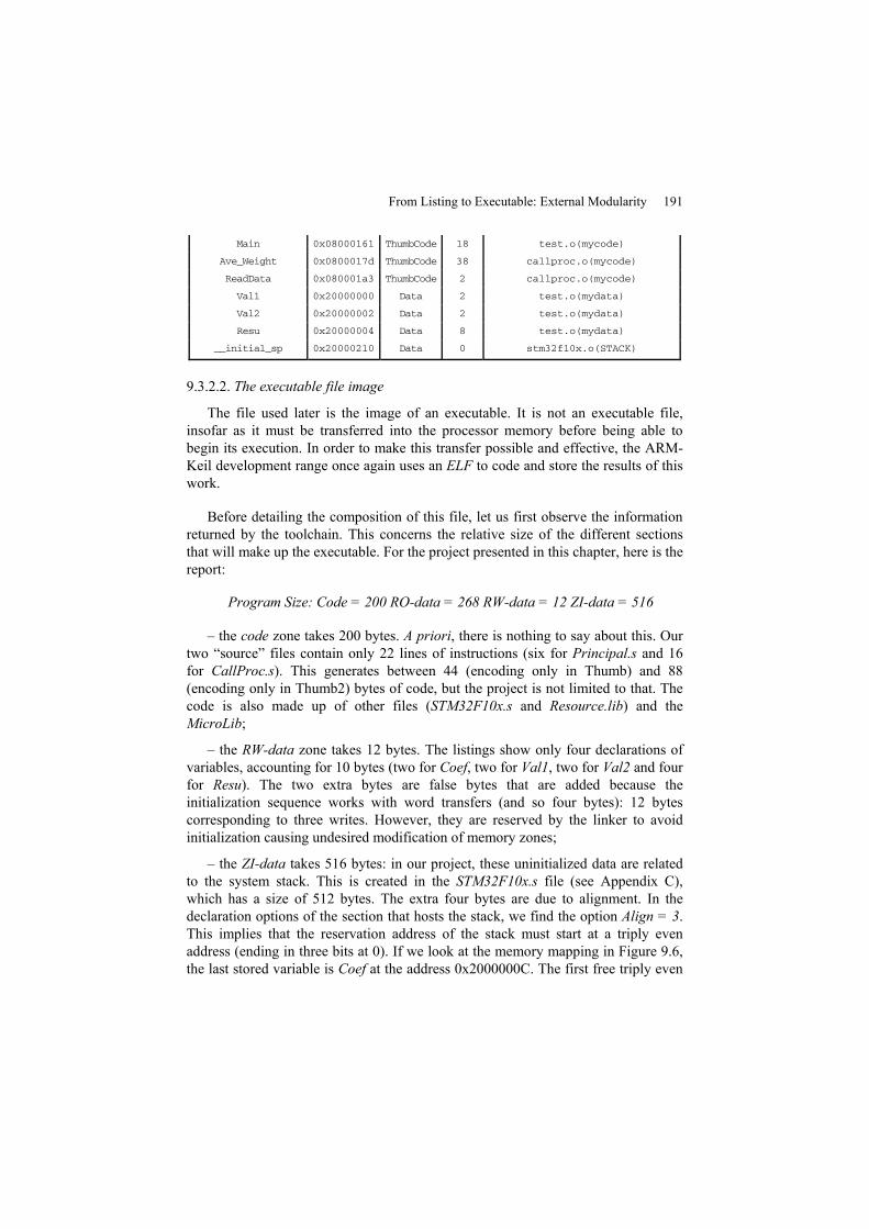
From Listing to Executable: External Modularity 191
Main 0x08000161 ThumbCode 18 test.o(mycode)
Ave_Weight 0x0800017d ThumbCode 38 callproc.o(mycode)
ReadData 0x080001a3 ThumbCode 2 callproc.o(mycode)
Val1 0x20000000 Data 2 test.o(mydata)
Val2 0x20000002 Data 2 test.o(mydata)
Resu 0x20000004 Data 8 test.o(mydata)
__initial_sp 0x20000210 Data 0 stm32f10x.o(STACK)
9.3.2.2. The executable file image
The file used later is the image of an executable. It is not an executable file,insofar as it must be transferred into the processor memory before being able tobegin its execution. In order to make this transfer possible and effective, the ARM-Keil development range once again uses an ELF to code and store the results of thiswork.
Before detailing the composition of this file, let us first observe the informationreturned by the toolchain. This concerns the relative size of the different sectionsthat will make up the executable. For the project presented in this chapter, here is thereport:
Program Size: Code = 200 RO-data = 268 RW-data = 12 ZI-data = 516
– the code zone takes 200 bytes. A priori, there is nothing to say about this. Ourtwo “source” files contain only 22 lines of instructions (six for Principal.s and 16for CallProc.s). This generates between 44 (encoding only in Thumb) and 88(encoding only in Thumb2) bytes of code, but the project is not limited to that. Thecode is also made up of other files (STM32F10x.s and Resource.lib) and theMicroLib;
– the RW-data zone takes 12 bytes. The listings show only four declarations ofvariables, accounting for 10 bytes (two for Coef, two for Val1, two for Val2 and fourfor Resu). The two extra bytes are false bytes that are added because theinitialization sequence works with word transfers (and so four bytes): 12 bytescorresponding to three writes. However, they are reserved by the linker to avoidinitialization causing undesired modification of memory zones;
– the ZI-data takes 516 bytes: in our project, these uninitialized data are relatedto the system stack. This is created in the STM32F10x.s file (see Appendix C),which has a size of 512 bytes. The extra four bytes are due to alignment. In thedeclaration options of the section that hosts the stack, we find the option Align = 3.This implies that the reservation address of the stack must start at a triply evenaddress (ending in three bits at 0). If we look at the memory mapping in Figure 9.6,the last stored variable is Coef at the address 0x2000000C. The first free triply even
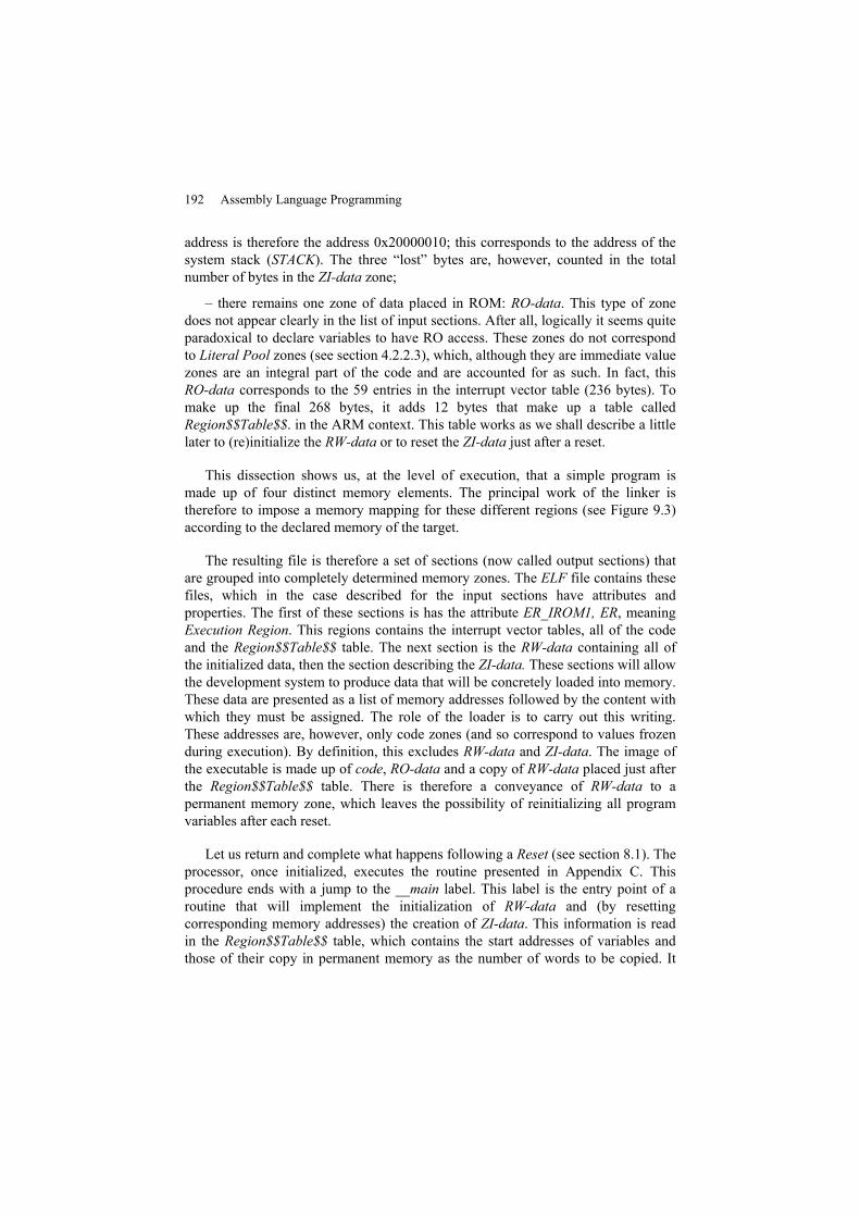
192 Assembly Language Programming
address is therefore the address 0x20000010; this corresponds to the address of thesystem stack (STACK). The three “lost” bytes are, however, counted in the totalnumber of bytes in the ZI-data zone;
– there remains one zone of data placed in ROM: RO-data. This type of zonedoes not appear clearly in the list of input sections. After all, logically it seems quiteparadoxical to declare variables to have RO access. These zones do not correspondto Literal Pool zones (see section 4.2.2.3), which, although they are immediate valuezones are an integral part of the code and are accounted for as such. In fact, thisRO-data corresponds to the 59 entries in the interrupt vector table (236 bytes). Tomake up the final 268 bytes, it adds 12 bytes that make up a table calledRegion$$Table$$. in the ARM context. This table works as we shall describe a littlelater to (re)initialize the RW-data or to reset the ZI-data just after a reset.
This dissection shows us, at the level of execution, that a simple program ismade up of four distinct memory elements. The principal work of the linker istherefore to impose a memory mapping for these different regions (see Figure 9.3)according to the declared memory of the target.
The resulting file is therefore a set of sections (now called output sections) thatare grouped into completely determined memory zones. The ELF file contains thesefiles, which in the case described for the input sections have attributes andproperties. The first of these sections is has the attribute ER_IROM1, ER, meaningExecution Region. This regions contains the interrupt vector tables, all of the codeand the Region$$Table$$ table. The next section is the RW-data containing all ofthe initialized data, then the section describing the ZI-data. These sections will allowthe development system to produce data that will be concretely loaded into memory.These data are presented as a list of memory addresses followed by the content withwhich they must be assigned. The role of the loader is to carry out this writing.These addresses are, however, only code zones (and so correspond to values frozenduring execution). By definition, this excludes RW-data and ZI-data. The image ofthe executable is made up of code, RO-data and a copy of RW-data placed just afterthe Region$$Table$$ table. There is therefore a conveyance of RW-data to apermanent memory zone, which leaves the possibility of reinitializing all programvariables after each reset.
Let us return and complete what happens following a Reset (see section 8.1). Theprocessor, once initialized, executes the routine presented in Appendix C. Thisprocedure ends with a jump to the __main label. This label is the entry point of aroutine that will implement the initialization of RW-data and (by resettingcorresponding memory addresses) the creation of ZI-data. This information is readin the Region$$Table$$ table, which contains the start addresses of variables andthose of their copy in permanent memory as the number of words to be copied. It
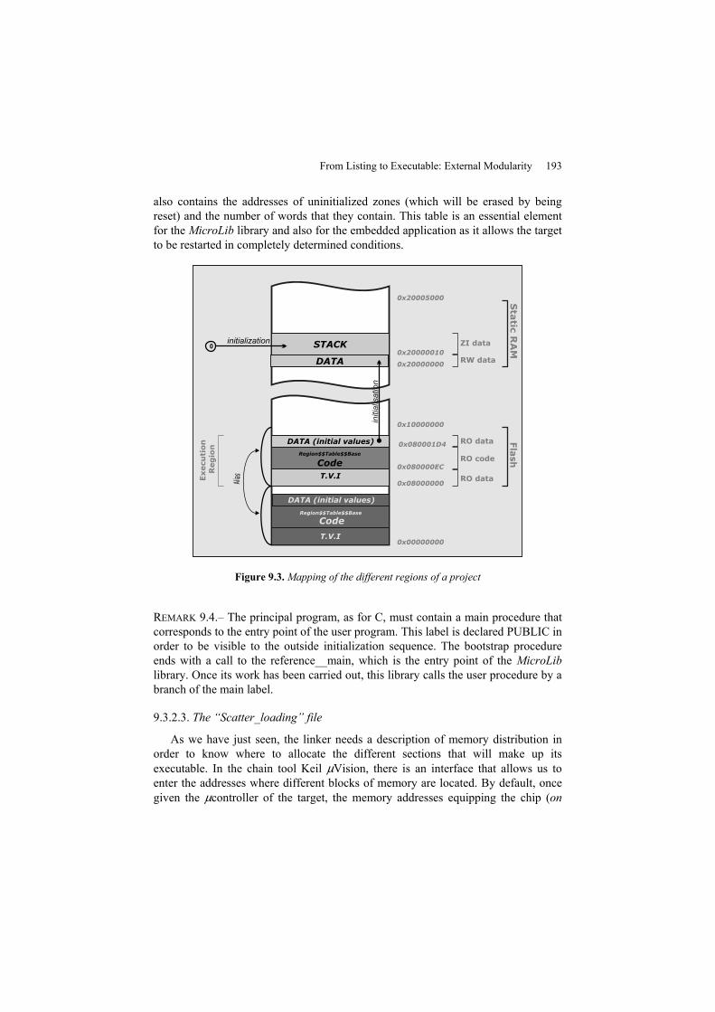
From Listing to Executable: External Modularity 193
also contains the addresses of uninitialized zones (which will be erased by beingreset) and the number of words that they contain. This table is an essential elementfor the MicroLib library and also for the embedded application as it allows the targetto be restarted in completely determined conditions.
DATA
STACK
DATA (initial values)
DATA (initial values)
T.V.I
T.V.I
0x20000000
0x20000010
0x20005000
RW data
RO data
Execu
tio
n
Reg
ion
RO data
RO code
ZI data
0x08000000
0x080000EC
0x080001D4
0x00000000
0x10000000
Code
Region$$Table$$Base
Code
Region$$Table$$Base
i nitia
l isatio
n
initialization0
Figure 9.3. Mapping of the different regions of a project
REMARK 9.4.– The principal program, as for C, must contain a main procedure thatcorresponds to the entry point of the user program. This label is declared PUBLIC inorder to be visible to the outside initialization sequence. The bootstrap procedureends with a call to the reference__main, which is the entry point of the MicroLiblibrary. Once its work has been carried out, this library calls the user procedure by abranch of the main label.
9.3.2.3. The “Scatter_loading” file
As we have just seen, the linker needs a description of memory distribution inorder to know where to allocate the different sections that will make up itsexecutable. In the chain tool Keil μVision, there is an interface that allows us toenter the addresses where different blocks of memory are located. By default, oncegiven the μcontroller of the target, the memory addresses equipping the chip (on
194 Assembly Language Programming
chip memory) are filled. If there are other memory devices present on the target, it isnecessary to supply their specifications, including the memory mapping.Nevertheless, the linker does not directly use the interface data but theScatter_loading file that is automatically generated by the interface. This file is atext file that describes the memory distribution formally and with its own syntax. Anadvanced user could perfectly edit and modify this file and bypass the interface todirectly inform the linker. This file is divided into three distinct regions:
– loading regions: these are the memory zones where code and RO-data will betransferred to memory. They can be multiple, although as in the case of the examplefor a simple executable, a single region is sufficient to hold all of the data to betransferred;
– execution regions: these are the regions where the code will be stored;
– read/write (RW) accessible regions: these are the regions where the programvariables will be stored.
For the presented example, the Scatter_loading file can reassemble the lines inExample 9.7.
EXAMPLE 9.7.– Example of a memory description file: a simple case
LR_IROM1 0x08000000 0x00020000 { ;
ER_IROM1 0x08000000 0x00020000 { ;
.ANY (+RO) ;
}
RW_IRAM1 0x20000000 0x00005000 { ;
.ANY (+RW +ZI) ;
}
}
Let us decipher these few lines:
– line delimits the loading region: the linker must generate an ELF file so thatthe list of addresses where the charger will make the transfers will be includedbetween 0x08000000 and 0x08020000. This region encompasses (the presence ofthe characters { and } encapsulates the declaration) all of the regions correspondingto different entities of the executable image;
– line indicates where address’s internal ROM memory is in the executionregion. In our case it involves the internal Flash of STM32, which corresponds to128 KB starting from address 0x08000000. It should be noted that this corresponds
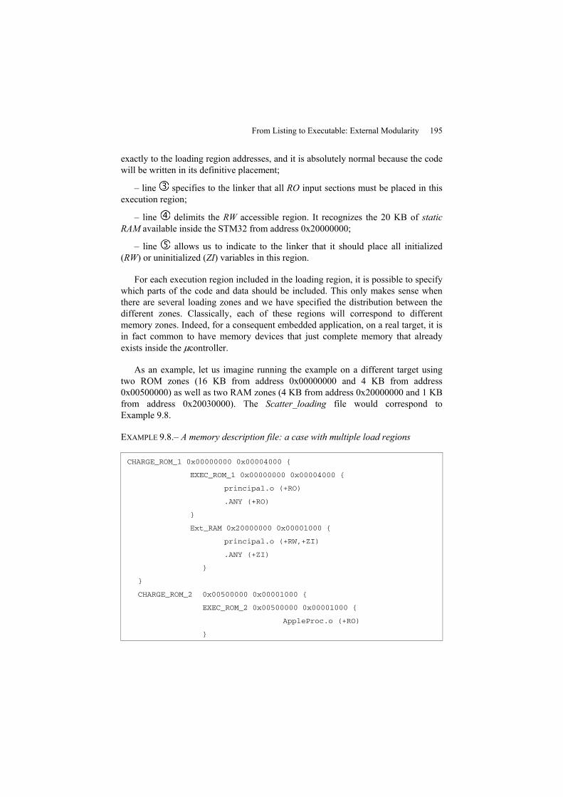
From Listing to Executable: External Modularity 195
exactly to the loading region addresses, and it is absolutely normal because the codewill be written in its definitive placement;
– line specifies to the linker that all RO input sections must be placed in thisexecution region;
– line delimits the RW accessible region. It recognizes the 20 KB of staticRAM available inside the STM32 from address 0x20000000;
– line allows us to indicate to the linker that it should place all initialized(RW) or uninitialized (ZI) variables in this region.
For each execution region included in the loading region, it is possible to specifywhich parts of the code and data should be included. This only makes sense whenthere are several loading zones and we have specified the distribution between thedifferent zones. Classically, each of these regions will correspond to differentmemory zones. Indeed, for a consequent embedded application, on a real target, it isin fact common to have memory devices that just complete memory that alreadyexists inside the μcontroller.
As an example, let us imagine running the example on a different target usingtwo ROM zones (16 KB from address 0x00000000 and 4 KB from address0x00500000) as well as two RAM zones (4 KB from address 0x20000000 and 1 KBfrom address 0x20030000). The Scatter_loading file would correspond toExample 9.8.
EXAMPLE 9.8.– A memory description file: a case with multiple load regions
CHARGE_ROM_1 0x00000000 0x00004000 {
EXEC_ROM_1 0x00000000 0x00004000 {
principal.o (+RO)
.ANY (+RO)
}
Ext_RAM 0x20000000 0x00001000 {
principal.o (+RW,+ZI)
.ANY (+ZI)
}
}
CHARGE_ROM_2 0x00500000 0x00001000 {
EXEC_ROM_2 0x00500000 0x00001000 {
AppleProc.o (+RO)
}
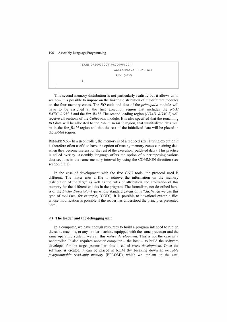
196 Assembly Language Programming
SRAM 0x20030000 0x00000400 {
AppleProc.o (+RW,+ZI)
.ANY (+RW)
}
}
This second memory distribution is not particularly realistic but it allows us tosee how it is possible to impose on the linker a distribution of the different moduleson the four memory zones. The RO code and data of the principal.o module willhave to be assigned at the first execution region that includes the ROMEXEC_ROM_1 and the Ext_RAM. The second loading region (LOAD_ROM_2) willreceive all sections of the CallProc.o module. It is also specified that the remainingRO data will be allocated to the EXEC_ROM_1 region, that uninitialized data willbe in the Ext_RAM region and that the rest of the initialized data will be placed inthe SRAM region.
REMARK 9.5.– In a μcontroller, the memory is of a reduced size. During execution itis therefore often useful to have the option of reusing memory zones containing datawhen they become useless for the rest of the execution (outdated data). This practiceis called overlay. Assembly language offers the option of superimposing variousdata sections in the same memory interval by using the COMMON direction (seesection 3.5.1).
In the case of development with the free GNU tools, the protocol used isdifferent. The linker uses a file to retrieve the information on the memorydistribution of the target as well as the rules of attribution and arbitration of thismemory for the different entities in the program. The formalism, not described here,is of the Linker Descriptor type whose standard extension is *.ld. When we use thistype of tool (see, for example, [COD]), it is possible to download example fileswhose modification is possible if the reader has understood the principles presentedhere.
9.4. The loader and the debugging unit
In a computer, we have enough resources to build a program intended to run onthe same machine, or any similar machine equipped with the same processor and thesame operating system; we call this native development. This is not the case in aμcontroller. It also requires another computer – the host – to build the softwaredeveloped for the target μcontroller: this is called cross development. Once thesoftware is created, it can be placed in ROM (by breaking down an erasableprogrammable read-only memory [EPROM]), which we implant on the card
From Listing to Executable: External Modularity 197
containing the μcontroller, but this approach is very inconvenient in the software-testing phase. We prefer to send it from the host to the μcontroller via a specializedconnection so that the host places the image of the executable itself in Flash memoryor RAM. This is no longer a load, but a download.
The “loader” program is responsible for properly copying the various sections ofthe program placed in the file containing the executable image to memory and then,if appropriate, launching the execution. This utility is included in most cross-development suites (such as toolchain).
The current generation of tools largely uses the JTAG (Joint Test Action Group)port standard to download programs directly to Flash memory. JTAG is asynchronous series bus standard. The JTAG debug adapter uses this protocol tocommunicate with the processor core. On a standard computer this bus is notpresent; the adapter will then communicate on the PC side with a classic connection(typically a Universal Serial Bus [USB]).
The development program or debugger is particularly useful for searching forerrors in a program. The program being reviewed runs under the control of thedebugger program. For this, the debugger obeys commands that the user has given itinline. This can launch the execution of the program in continuous mode or step-by-step mode: in the latter case, only a single instruction of the program is executed andthe debugger takes back control. The user can place a breakpoint on an instructionof the program being reviewed before launching the execution of the program: thiswill interrupt the execution just before this instruction. At each stop in the program,the debugger provides the current contents of all registers of the processor, and theuser can then find out the current state of the program; he/she can also look at thecontents of the system stack or any other memory region. Thus he/she can know thecurrent value of a datum for which he/she knows the address (thanks to the symboltable given by the linker), or for which he/she gives the name if the debugger issymbolic. At each time the program is stopped, the debugger also allows us tochange the value contained in any register, or to change any variable or memoryposition, before resuming the execution.
Note that to do its job, a symbolic debugger must at least have the symbol table.In fact, all debuggers need a range of information that must be included in theexecutable file. For this, the programmer must indicate (by invoking the assemblerand linker with specific options) that they must include the information necessaryfor development under the debugger.
As was presented in Chapter 1 on Cortex architecture (see section 1.2.1.2), thereare several hardware units whose roles consist mainly of returning information to ahost system without having any effect on the running of the program being
198 Assembly Language Programming
executed. This can typically be achieved with the Trace Macrocell units that can, inreal-time and without causing any alteration of the processor, analyze and transmitdata on the behavior and performance of the target thus observed. This approach,known as non-intrusive in ARM documentation, is particularly interesting forsystem surveillance, or in the case of dysfunction that is particularly difficult tolocalize or explain.
In a classic development cycle, the first development steps require a much moreintrusive approach, such as placing a breakpoint at a specified code address to stopthe sequence during execution, analyzing the state of the processor at that precisemoment, and then possibly resuming the execution step-by-step.
Cortex-M3 architecture offers two versions of these intrusive techniques:
– the first technique involves freezing the processor core at the software level.Cortex-M3 then switches to an internal state call Debug State, in which it is possibleto specify the step-by-step running of the program being executed, among otherthings. The development system, via the JTAG port, acts (by RW) directly on theregisters of the debugging units and allows control from outside the program that isrunning;
– the second, less intrusive approach consists of using a Debug Monitor, whichis a software application embedded in Cortex-M3 that is triggered by an exception(see section 8.2.1.6). The exception then takes control of the running of the sequenceexecuted by the processor and communicates with the development unit.
As the objectives of this book do not include a deep and thorough understandingof all aspects of Cortex-M3, we will not further explain the methods and internalarchitectures involved in debugging. It is nevertheless true that “lower-level”programming cannot be done without these development tools, if only because theprogrammer has no other way of observing what happens in the target.

APPENDICES

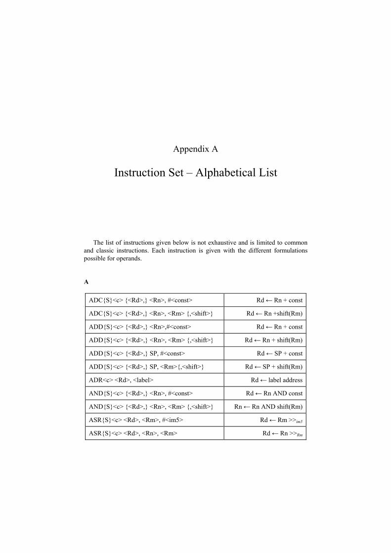
Appendix A
Instruction Set – Alphabetical List
The list of instructions given below is not exhaustive and is limited to commonand classic instructions. Each instruction is given with the different formulationspossible for operands.
A
ADC{S}<c> {<Rd>,} <Rn>, #<const> Rd← Rn + const
ADC{S}<c> {<Rd>,} <Rn>, <Rm> {,<shift>} Rd← Rn +shift(Rm)
ADD{S}<c> {<Rd>,} <Rn>,#<const> Rd← Rn + const
ADD{S}<c> {<Rd>,} <Rn>, <Rm> {,<shift>} Rd← Rn + shift(Rm)
ADD{S}<c> {<Rd>,} SP, #<const> Rd← SP + const
ADD{S}<c> {<Rd>,} SP, <Rm>{,<shift>} Rd← SP + shift(Rm)
ADR<c> <Rd>, <label> Rd← label address
AND{S}<c> {<Rd>,} <Rn>, #<const> Rd← Rn AND const
AND{S}<c> {<Rd>,} <Rn>, <Rm> {,<shift>} Rn← Rn AND shift(Rm)
ASR{S}<c> <Rd>, <Rm>, #<im5> Rd← Rm >>im5
ASR{S}<c> <Rd>, <Rn>, <Rm> Rd← Rn >>Rm
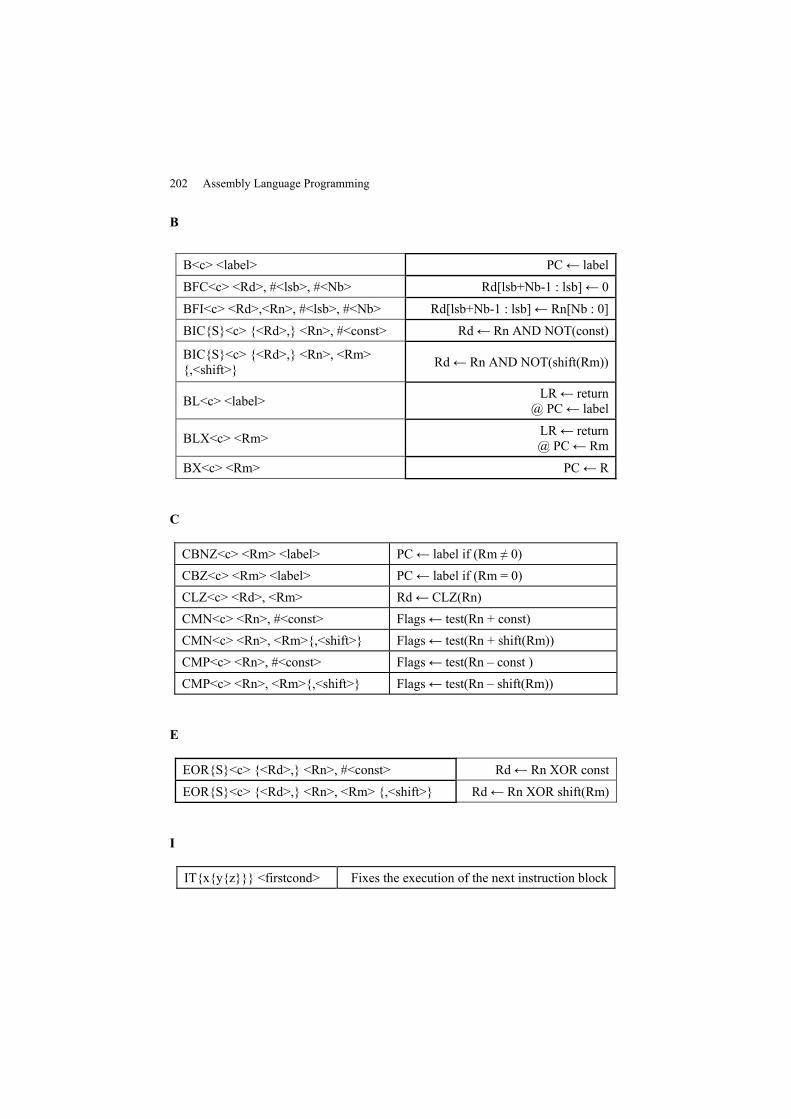
202 Assembly Language Programming
B
B<c> <label> PC← label
BFC<c> <Rd>, #<lsb>, #<Nb> Rd[lsb+Nb-1 : lsb]← 0
BFI<c> <Rd>,<Rn>, #<lsb>, #<Nb> Rd[lsb+Nb-1 : lsb]← Rn[Nb : 0]
BIC{S}<c> {<Rd>,} <Rn>, #<const> Rd← Rn AND NOT(const)
BIC{S}<c> {<Rd>,} <Rn>, <Rm>{,<shift>} Rd← Rn AND NOT(shift(Rm))
BL<c> <label> LR← return@ PC← label
BLX<c> <Rm> LR← return@ PC← Rm
BX<c> <Rm> PC← R
C
CBNZ<c> <Rm> <label> PC← label if (Rm ≠ 0)CBZ<c> <Rm> <label> PC← label if (Rm = 0)CLZ<c> <Rd>, <Rm> Rd← CLZ(Rn)CMN<c> <Rn>, #<const> Flags← test(Rn + const)CMN<c> <Rn>, <Rm>{,<shift>} Flags← test(Rn + shift(Rm))CMP<c> <Rn>, #<const> Flags← test(Rn – const )CMP<c> <Rn>, <Rm>{,<shift>} Flags← test(Rn – shift(Rm))
E
EOR{S}<c> {<Rd>,} <Rn>, #<const> Rd← Rn XOR const
EOR{S}<c> {<Rd>,} <Rn>, <Rm> {,<shift>} Rd← Rn XOR shift(Rm)
I
IT{x{y{z}}} <firstcond> Fixes the execution of the next instruction block
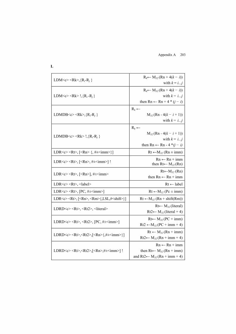
Appendix A 203
L
LDM<c> <Rk>,{Ri-Rj }Rk←M32 (Rn + 4(k − i))
with k = i...j
LDM<c> <Rk> !,{Ri -Rj }Rk←M32 (Rn + 4(k − i))
with k = i...jthen Rn← Rn + 4 * (j − i)
LDMDB<c> <Rk>,{Ri-Rj }Rk ←
M32 (Rn - 4(k − i + 1))with k = i...j
LDMDB<c> <Rk> !,{Ri-Rj }
Rk ←M32 (Rn - 4(k − i + 1))
with k = i...jthen Rn← Rn - 4 *(j − i)
LDR<c> <Rt>, [<Rn> {, #±<imm>}] Rt←M32 (Rn ± imm)
LDR<c> <Rt>, [<Rn>, #±<imm>] ! Rn← Rn + immthen Rt←M32 (Rn)
LDR<c> <Rt>, [<Rn>], #±<imm>Rt←M32 (Rn)
then Rn← Rn + imm
LDR<c> <Rt>, <label> Rt← label
LDR<c> <Rt>, [PC, #±<imm>] Rt←M32 (Pc ± imm)
LDR<c> <Rt>, [<Rn>, <Rm>{,LSL,#<shift>}] Rt←M32 (Rn + shift(Rm))
LDRD<c> <Rt>, <Rt2>, <literal>Rt←M32 (literal)
Rt2←M32 (literal + 4)
LDRD<c> <Rt>, <Rt2>, [PC, #±<imm>]Rt←M32 (PC + imm)
Rt2←M32 (PC + imm + 4)
LDRD<c> <Rt>,<Rt2>,[<Rn>{,#±<imm>}]Rt←M32 (Rn + imm)
Rt2←M32 (Rn + imm + 4)
LDRD<c> <Rt>,<Rt2>,[<Rn>,#±<imm>] !Rn← Rn + imm
then Rt←M32 (Rn + imm)and Rt2←M32 (Rn + imm + 4)
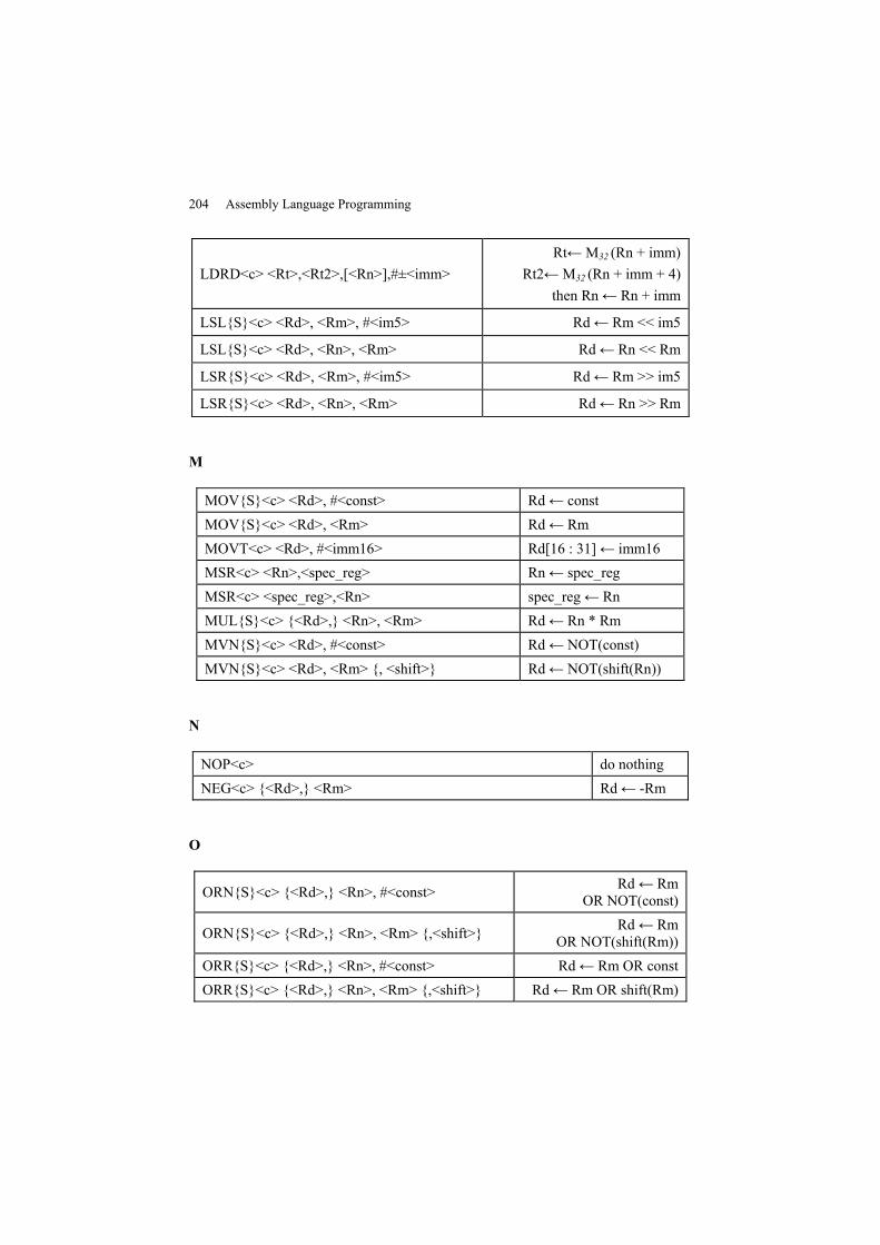
204 Assembly Language Programming
LDRD<c> <Rt>,<Rt2>,[<Rn>],#±<imm>Rt←M32 (Rn + imm)
Rt2←M32 (Rn + imm + 4)then Rn← Rn + imm
LSL{S}<c> <Rd>, <Rm>, #<im5> Rd← Rm << im5
LSL{S}<c> <Rd>, <Rn>, <Rm> Rd← Rn << Rm
LSR{S}<c> <Rd>, <Rm>, #<im5> Rd← Rm >> im5
LSR{S}<c> <Rd>, <Rn>, <Rm> Rd← Rn >> Rm
M
MOV{S}<c> <Rd>, #<const> Rd← constMOV{S}<c> <Rd>, <Rm> Rd← RmMOVT<c> <Rd>, #<imm16> Rd[16 : 31]← imm16MSR<c> <Rn>,<spec_reg> Rn← spec_regMSR<c> <spec_reg>,<Rn> spec_reg← RnMUL{S}<c> {<Rd>,} <Rn>, <Rm> Rd← Rn * RmMVN{S}<c> <Rd>, #<const> Rd← NOT(const)MVN{S}<c> <Rd>, <Rm> {, <shift>} Rd← NOT(shift(Rn))
N
NOP<c> do nothingNEG<c> {<Rd>,} <Rm> Rd← -Rm
O
ORN{S}<c> {<Rd>,} <Rn>, #<const> Rd← RmOR NOT(const)
ORN{S}<c> {<Rd>,} <Rn>, <Rm> {,<shift>} Rd← RmOR NOT(shift(Rm))
ORR{S}<c> {<Rd>,} <Rn>, #<const> Rd← Rm OR constORR{S}<c> {<Rd>,} <Rn>, <Rm> {,<shift>} Rd← Rm OR shift(Rm)
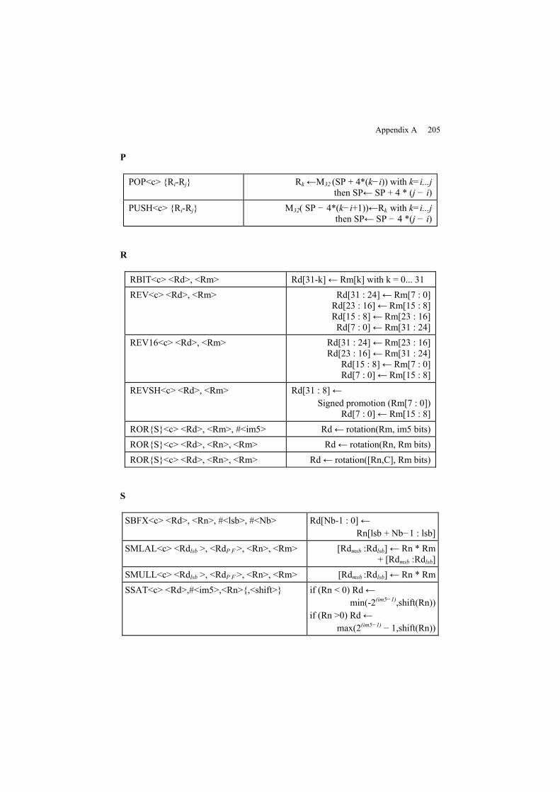
Appendix A 205
P
POP<c> {Ri-Rj} Rk ←M32 (SP + 4*(k−i)) with k=i...jthen SP← SP + 4 * (j − i)
PUSH<c> {Ri-Rj} M32( SP − 4*(k−i+1))←Rk with k=i...jthen SP← SP − 4 *(j − i)
R
RBIT<c> <Rd>, <Rm> Rd[31-k]← Rm[k] with k = 0... 31REV<c> <Rd>, <Rm> Rd[31 : 24]← Rm[7 : 0]
Rd[23 : 16]← Rm[15 : 8]Rd[15 : 8]← Rm[23 : 16]Rd[7 : 0]← Rm[31 : 24]
REV16<c> <Rd>, <Rm> Rd[31 : 24]← Rm[23 : 16]Rd[23 : 16]← Rm[31 : 24]
Rd[15 : 8]← Rm[7 : 0]Rd[7 : 0]← Rm[15 : 8]
REVSH<c> <Rd>, <Rm> Rd[31 : 8]←Signed promotion (Rm[7 : 0])
Rd[7 : 0]← Rm[15 : 8]ROR{S}<c> <Rd>, <Rm>, #<im5> Rd← rotation(Rm, im5 bits)ROR{S}<c> <Rd>, <Rn>, <Rm> Rd← rotation(Rn, Rm bits)ROR{S}<c> <Rd>, <Rn>, <Rm> Rd← rotation([Rn,C], Rm bits)
S
SBFX<c> <Rd>, <Rn>, #<lsb>, #<Nb> Rd[Nb-1 : 0]←Rn[lsb + Nb−1 : lsb]
SMLAL<c> <Rdlsb >, <RdP F>, <Rn>, <Rm> [Rdmsb :Rdlsb]← Rn * Rm+ [Rdmsb :Rdlsb]
SMULL<c> <Rdlsb >, <RdP F>, <Rn>, <Rm> [Rdmsb :Rdlsb]← Rn * RmSSAT<c> <Rd>,#<im5>,<Rn>{,<shift>} if (Rn < 0) Rd←
min(-2(im5−1),shift(Rn))if (Rn >0) Rd←
max(2(im5−1) − 1,shift(Rn))
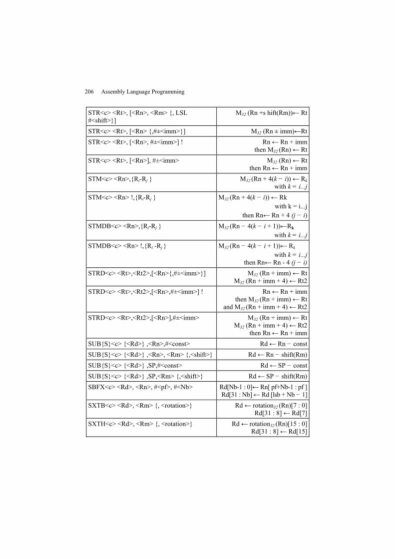
206 Assembly Language Programming
STR<c> <Rt>, [<Rn>, <Rm> {, LSL#<shift>}]
M32 (Rn +s hift(Rm))← Rt
STR<c> <Rt>, [<Rn> {,#±<imm>}] M32 (Rn ± imm)←RtSTR<c> <Rt>, [<Rn>, #±<imm>] ! Rn← Rn + imm
then M32 (Rn)← RtSTR<c> <Rt>, [<Rn>], #±<imm> M32 (Rn)← Rt
then Rn← Rn + immSTM<c> <Rn>,{Ri-Rj } M32 (Rn + 4(k − i))← Rk
with k = i...jSTM<c> <Rn> !,{Ri-Rj } M32 (Rn + 4(k − i))← Rk
with k = i...jthen Rn← Rn + 4 (j − i)
STMDB<c> <Rn>,{Ri-Rj } M32 (Rn − 4(k − i + 1))←Rk
with k = i...jSTMDB<c> <Rn> !,{Ri -Rj } M32 (Rn − 4(k − i + 1))← Rk
with k = i...jthen Rn← Rn - 4 (j − i)
STRD<c> <Rt>,<Rt2>,[<Rn>{,#±<imm>}] M32 (Rn + imm)← RtM32 (Rn + imm + 4)← Rt2
STRD<c> <Rt>,<Rt2>,[<Rn>,#±<imm>] ! Rn← Rn + immthen M32 (Rn + imm)← Rt
and M32 (Rn + imm + 4)← Rt2STRD<c> <Rt>,<Rt2>,[<Rn>],#±<imm> M32 (Rn + imm)← Rt
M32 (Rn + imm + 4)← Rt2then Rn← Rn + imm
SUB{S}<c> {<Rd>} ,<Rn>,#<const> Rd← Rn − constSUB{S}<c> {<Rd>} ,<Rn>, <Rm> {,<shift>} Rd← Rn − shift(Rm)SUB{S}<c> {<Rd>} ,SP,#<const> Rd← SP − constSUB{S}<c> {<Rd>} ,SP,<Rm> {,<shift>} Rd← SP − shift(Rm)SBFX<c> <Rd>, <Rn>, #<pf>, #<Nb> Rd[Nb-1 : 0]← Rn[ pf+Nb-1 : pf ]
Rd[31 : Nb]← Rd [lsb + Nb − 1]SXTB<c> <Rd>, <Rm> {, <rotation>} Rd← rotation32 (Rn)[7 : 0]
Rd[31 : 8]← Rd[7]SXTH<c> <Rd>, <Rm> {, <rotation>} Rd← rotation32 (Rn)[15 : 0]
Rd[31 : 8]← Rd[15]
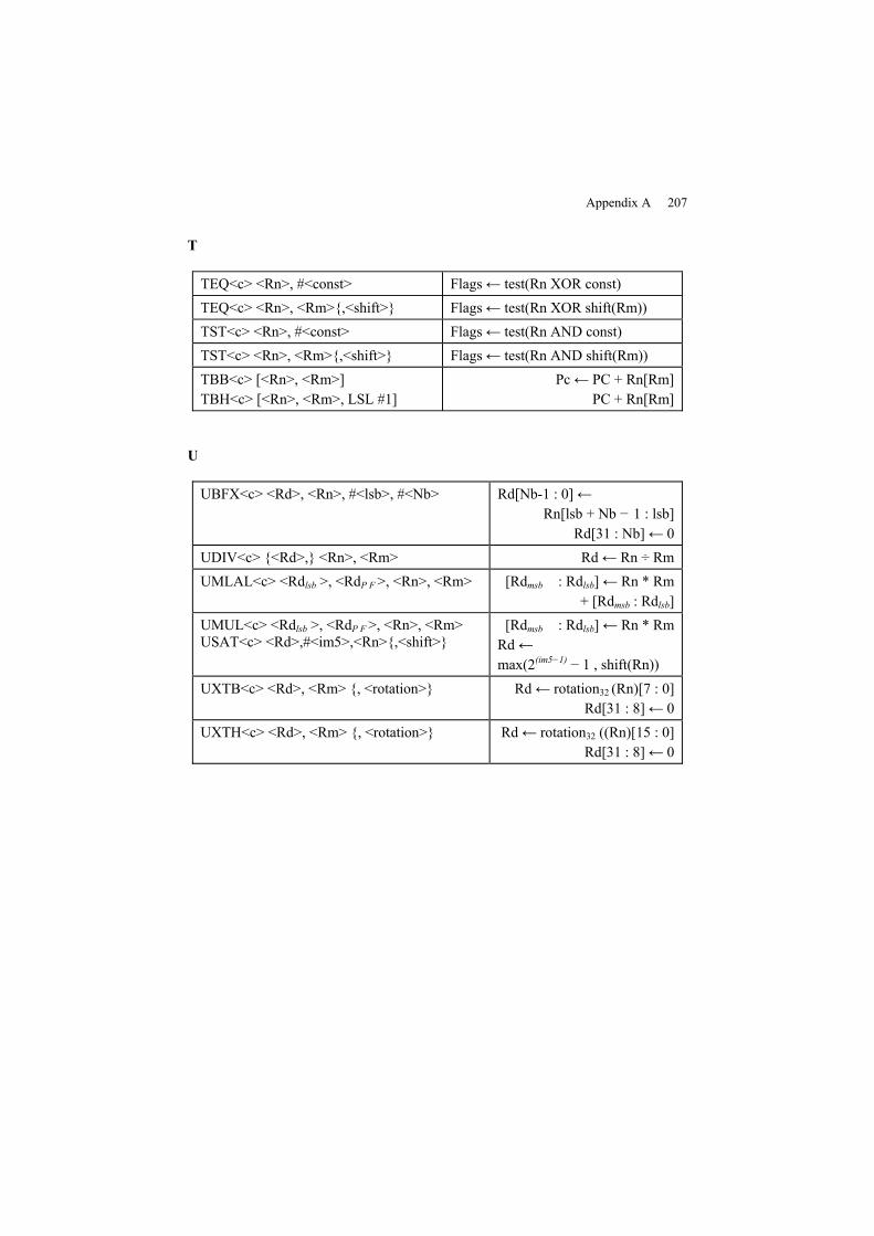
Appendix A 207
T
TEQ<c> <Rn>, #<const> Flags← test(Rn XOR const)TEQ<c> <Rn>, <Rm>{,<shift>} Flags← test(Rn XOR shift(Rm))TST<c> <Rn>, #<const> Flags← test(Rn AND const)TST<c> <Rn>, <Rm>{,<shift>} Flags← test(Rn AND shift(Rm))TBB<c> [<Rn>, <Rm>]TBH<c> [<Rn>, <Rm>, LSL #1]
Pc← PC + Rn[Rm]PC + Rn[Rm]
U
UBFX<c> <Rd>, <Rn>, #<lsb>, #<Nb> Rd[Nb-1 : 0]←Rn[lsb + Nb − 1 : lsb]
Rd[31 : Nb]← 0UDIV<c> {<Rd>,} <Rn>, <Rm> Rd← Rn ÷ RmUMLAL<c> <Rdlsb >, <RdP F>, <Rn>, <Rm> [Rdmsb : Rdlsb]← Rn * Rm
+ [Rdmsb : Rdlsb]UMUL<c> <Rdlsb >, <RdP F>, <Rn>, <Rm>USAT<c> <Rd>,#<im5>,<Rn>{,<shift>}
[Rdmsb : Rdlsb]← Rn * RmRd←max(2(im5−1) − 1 , shift(Rn))
UXTB<c> <Rd>, <Rm> {, <rotation>} Rd← rotation32 (Rn)[7 : 0]Rd[31 : 8]← 0
UXTH<c> <Rd>, <Rm> {, <rotation>} Rd← rotation32 ((Rn)[15 : 0]Rd[31 : 8]← 0

Appendix B
The SysTick Timer
B.1. Counters and timers in general
Counters and timers are two entities that we must encounter in a μcontroller.They both do exactly the same thing. Indeed they correspond to registers that countup or down and have rising or descending fronts, or both. The difference betweenthe two names is that, in the case of timers, the front sequence that supplies the unitis periodic and has a known period (which is often adjustable). This implies that thevalue contained within the register corresponds to a time measurement, hence itsname.
The main event that occurs in the process of incrementation (or decrementation,respectively) is the overflow (or underflow) of the capacity of the register. Manythings can intervene in this event but the main two programmable actions onoverflow (underflow) are sending an interrupt request and reloading a given value inthe counting register, causing a sample call to a specific routine. This functionality isnecessary for the development of a real-time kernel whose main role is sharingcentral processing unit (CPU) time between different tasks running on the processor.The motivation for the Advanced RISC Machine’s (ARM’s) choice to provide atimer inside the core was to be free from the specificities of the μcontrollers (and soto be free from the choice of developers) so that a real-time kernel base could bedeveloped for all of the circuits based on Cortex-M3. On its website, ARM lists thepartners proposing such a real-time kernels (Real-Time Operating Systems) – thereare over 20, and the list is subject to frequent change.
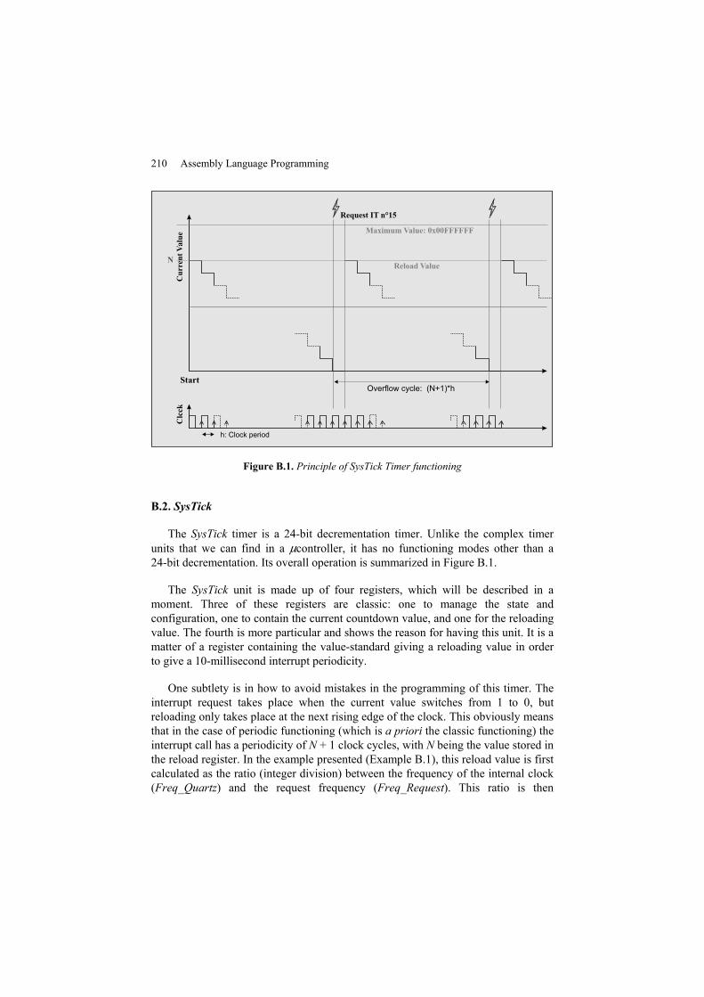
210 Assembly Language Programming
N
Request IT n°15
Start
h: Clock period
Overflow cycle: (N+1)*h
Cu
rren
tV
alu
eC
lcck
Maximum Value: 0x00FFFFFF
Reload Value
Figure B.1. Principle of SysTick Timer functioning
B.2. SysTick
The SysTick timer is a 24-bit decrementation timer. Unlike the complex timerunits that we can find in a μcontroller, it has no functioning modes other than a24-bit decrementation. Its overall operation is summarized in Figure B.1.
The SysTick unit is made up of four registers, which will be described in amoment. Three of these registers are classic: one to manage the state andconfiguration, one to contain the current countdown value, and one for the reloadingvalue. The fourth is more particular and shows the reason for having this unit. It is amatter of a register containing the value-standard giving a reloading value in orderto give a 10-millisecond interrupt periodicity.
One subtlety is in how to avoid mistakes in the programming of this timer. Theinterrupt request takes place when the current value switches from 1 to 0, butreloading only takes place at the next rising edge of the clock. This obviously meansthat in the case of periodic functioning (which is a priori the classic functioning) theinterrupt call has a periodicity of N + 1 clock cycles, with N being the value stored inthe reload register. In the example presented (Example B.1), this reload value is firstcalculated as the ratio (integer division) between the frequency of the internal clock(Freq_Quartz) and the request frequency (Freq_Request). This ratio is then
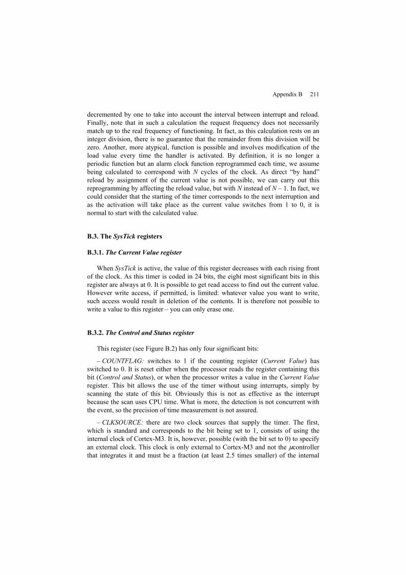
Appendix B 211
decremented by one to take into account the interval between interrupt and reload.Finally, note that in such a calculation the request frequency does not necessarilymatch up to the real frequency of functioning. In fact, as this calculation rests on aninteger division, there is no guarantee that the remainder from this division will bezero. Another, more atypical, function is possible and involves modification of theload value every time the handler is activated. By definition, it is no longer aperiodic function but an alarm clock function reprogrammed each time, we assumebeing calculated to correspond with N cycles of the clock. As direct “by hand”reload by assignment of the current value is not possible, we can carry out thisreprogramming by affecting the reload value, but with N instead of N – 1. In fact, wecould consider that the starting of the timer corresponds to the next interruption andas the activation will take place as the current value switches from 1 to 0, it isnormal to start with the calculated value.
B.3. The SysTick registers
B.3.1. The Current Value register
When SysTick is active, the value of this register decreases with each rising frontof the clock. As this timer is coded in 24 bits, the eight most significant bits in thisregister are always at 0. It is possible to get read access to find out the current value.However write access, if permitted, is limited: whatever value you want to write,such access would result in deletion of the contents. It is therefore not possible towrite a value to this register – you can only erase one.
B.3.2. The Control and Status register
This register (see Figure B.2) has only four significant bits:
– COUNTFLAG: switches to 1 if the counting register (Current Value) hasswitched to 0. It is reset either when the processor reads the register containing thisbit (Control and Status), or when the processor writes a value in the Current Valueregister. This bit allows the use of the timer without using interrupts, simply byscanning the state of this bit. Obviously this is not as effective as the interruptbecause the scan uses CPU time. What is more, the detection is not concurrent withthe event, so the precision of time measurement is not assured.
– CLKSOURCE: there are two clock sources that supply the timer. The first,which is standard and corresponds to the bit being set to 1, consists of using theinternal clock of Cortex-M3. It is, however, possible (with the bit set to 0) to specifyan external clock. This clock is only external to Cortex-M3 and not the μcontrollerthat integrates it and must be a fraction (at least 2.5 times smaller) of the internal
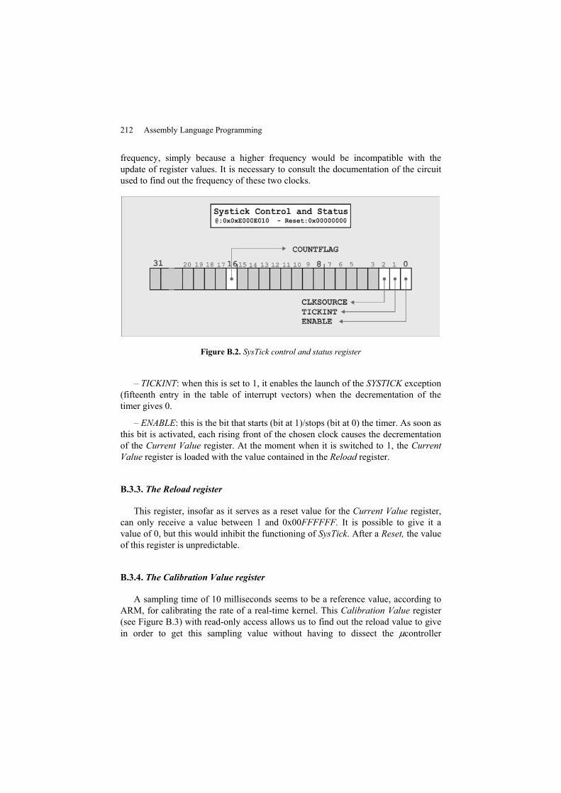
212 Assembly Language Programming
frequency, simply because a higher frequency would be incompatible with theupdate of register values. It is necessary to consult the documentation of the circuitused to find out the frequency of these two clocks.
Figure B.2. SysTick control and status register
– TICKINT: when this is set to 1, it enables the launch of the SYSTICK exception(fifteenth entry in the table of interrupt vectors) when the decrementation of thetimer gives 0.
– ENABLE: this is the bit that starts (bit at 1)/stops (bit at 0) the timer. As soon asthis bit is activated, each rising front of the chosen clock causes the decrementationof the Current Value register. At the moment when it is switched to 1, the CurrentValue register is loaded with the value contained in the Reload register.
B.3.3. The Reload register
This register, insofar as it serves as a reset value for the Current Value register,can only receive a value between 1 and 0x00FFFFFF. It is possible to give it avalue of 0, but this would inhibit the functioning of SysTick. After a Reset, the valueof this register is unpredictable.
B.3.4. The Calibration Value register
A sampling time of 10 milliseconds seems to be a reference value, according toARM, for calibrating the rate of a real-time kernel. This Calibration Value register(see Figure B.3) with read-only access allows us to find out the reload value to givein order to get this sampling value without having to dissect the μcontroller
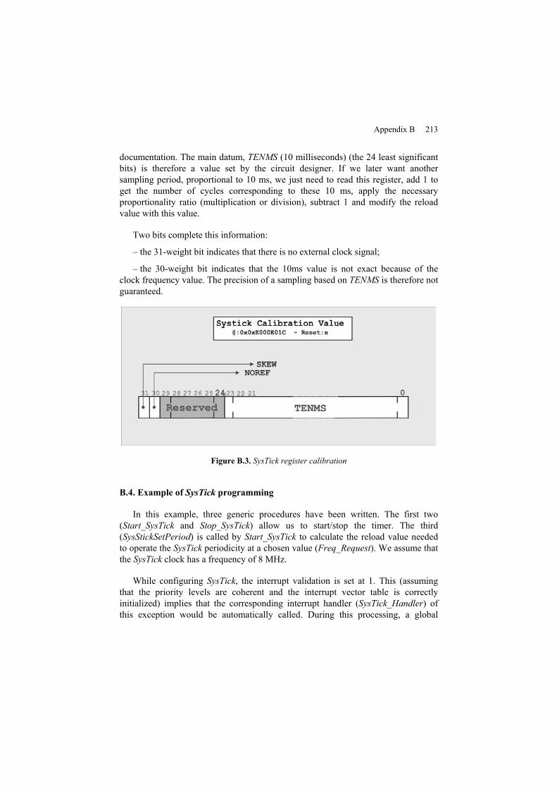
Appendix B 213
documentation. The main datum, TENMS (10 milliseconds) (the 24 least significantbits) is therefore a value set by the circuit designer. If we later want anothersampling period, proportional to 10 ms, we just need to read this register, add 1 toget the number of cycles corresponding to these 10 ms, apply the necessaryproportionality ratio (multiplication or division), subtract 1 and modify the reloadvalue with this value.
Two bits complete this information:
– the 31-weight bit indicates that there is no external clock signal;
– the 30-weight bit indicates that the 10ms value is not exact because of theclock frequency value. The precision of a sampling based on TENMS is therefore notguaranteed.
Figure B.3. SysTick register calibration
B.4. Example of SysTick programming
In this example, three generic procedures have been written. The first two(Start_SysTick and Stop_SysTick) allow us to start/stop the timer. The third(SysStickSetPeriod) is called by Start_SysTick to calculate the reload value neededto operate the SysTick periodicity at a chosen value (Freq_Request). We assume thatthe SysTick clock has a frequency of 8 MHz.
While configuring SysTick, the interrupt validation is set at 1. This (assumingthat the priority levels are coherent and the interrupt vector table is correctlyinitialized) implies that the corresponding interrupt handler (SysTick_Handler) ofthis exception would be automatically called. During this processing, a global
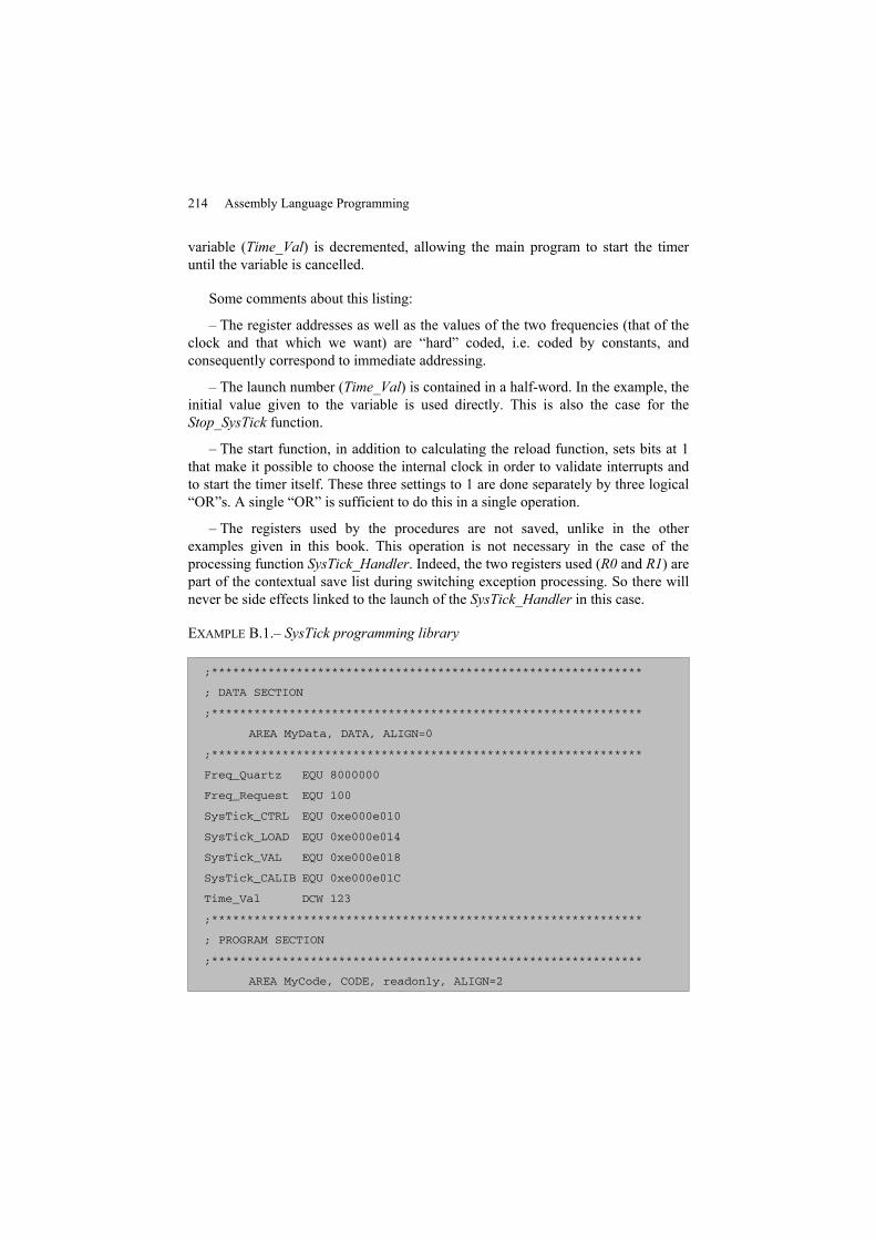
214 Assembly Language Programming
variable (Time_Val) is decremented, allowing the main program to start the timeruntil the variable is cancelled.
Some comments about this listing:
– The register addresses as well as the values of the two frequencies (that of theclock and that which we want) are “hard” coded, i.e. coded by constants, andconsequently correspond to immediate addressing.
– The launch number (Time_Val) is contained in a half-word. In the example, theinitial value given to the variable is used directly. This is also the case for theStop_SysTick function.
– The start function, in addition to calculating the reload function, sets bits at 1that make it possible to choose the internal clock in order to validate interrupts andto start the timer itself. These three settings to 1 are done separately by three logical“OR”s. A single “OR” is sufficient to do this in a single operation.
– The registers used by the procedures are not saved, unlike in the otherexamples given in this book. This operation is not necessary in the case of theprocessing function SysTick_Handler. Indeed, the two registers used (R0 and R1) arepart of the contextual save list during switching exception processing. So there willnever be side effects linked to the launch of the SysTick_Handler in this case.
EXAMPLE B.1.– SysTick programming library
;*************************************************************
; DATA SECTION
;*************************************************************
AREA MyData, DATA, ALIGN=0
;*************************************************************
Freq_Quartz EQU 8000000
Freq_Request EQU 100
SysTick_CTRL EQU 0xe000e010
SysTick_LOAD EQU 0xe000e014
SysTick_VAL EQU 0xe000e018
SysTick_CALIB EQU 0xe000e01C
Time_Val DCW 123
;*************************************************************
; PROGRAM SECTION
;*************************************************************
AREA MyCode, CODE, readonly, ALIGN=2
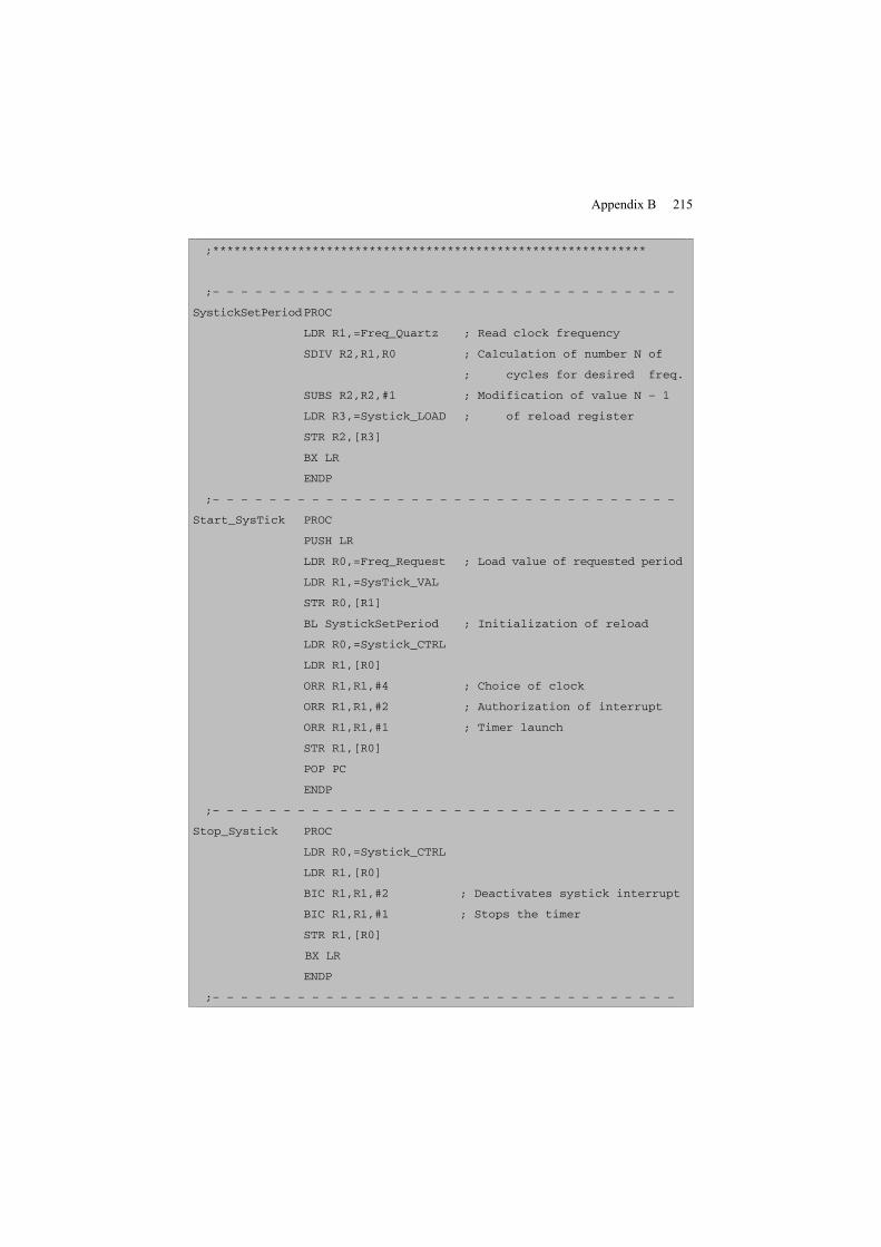
Appendix B 215
;*************************************************************
;– – – – – – – – – – – – – – – – – – – – – – – – – – – – – – – – –
SystickSetPeriodPROC
LDR R1,=Freq_Quartz ; Read clock frequency
SDIV R2,R1,R0 ; Calculation of number N of
; cycles for desired freq.
SUBS R2,R2,#1 ; Modification of value N – 1
LDR R3,=Systick_LOAD ; of reload register
STR R2,[R3]
BX LR
ENDP
;– – – – – – – – – – – – – – – – – – – – – – – – – – – – – – – – –
Start_SysTick PROC
PUSH LR
LDR R0,=Freq_Request ; Load value of requested period
LDR R1,=SysTick_VAL
STR R0,[R1]
BL SystickSetPeriod ; Initialization of reload
LDR R0,=Systick_CTRL
LDR R1,[R0]
ORR R1,R1,#4 ; Choice of clock
ORR R1,R1,#2 ; Authorization of interrupt
ORR R1,R1,#1 ; Timer launch
STR R1,[R0]
POP PC
ENDP
;– – – – – – – – – – – – – – – – – – – – – – – – – – – – – – – – –
Stop_Systick PROC
LDR R0,=Systick_CTRL
LDR R1,[R0]
BIC R1,R1,#2 ; Deactivates systick interrupt
BIC R1,R1,#1 ; Stops the timer
STR R1,[R0]
BX LR
ENDP
;– – – – – – – – – – – – – – – – – – – – – – – – – – – – – – – – –
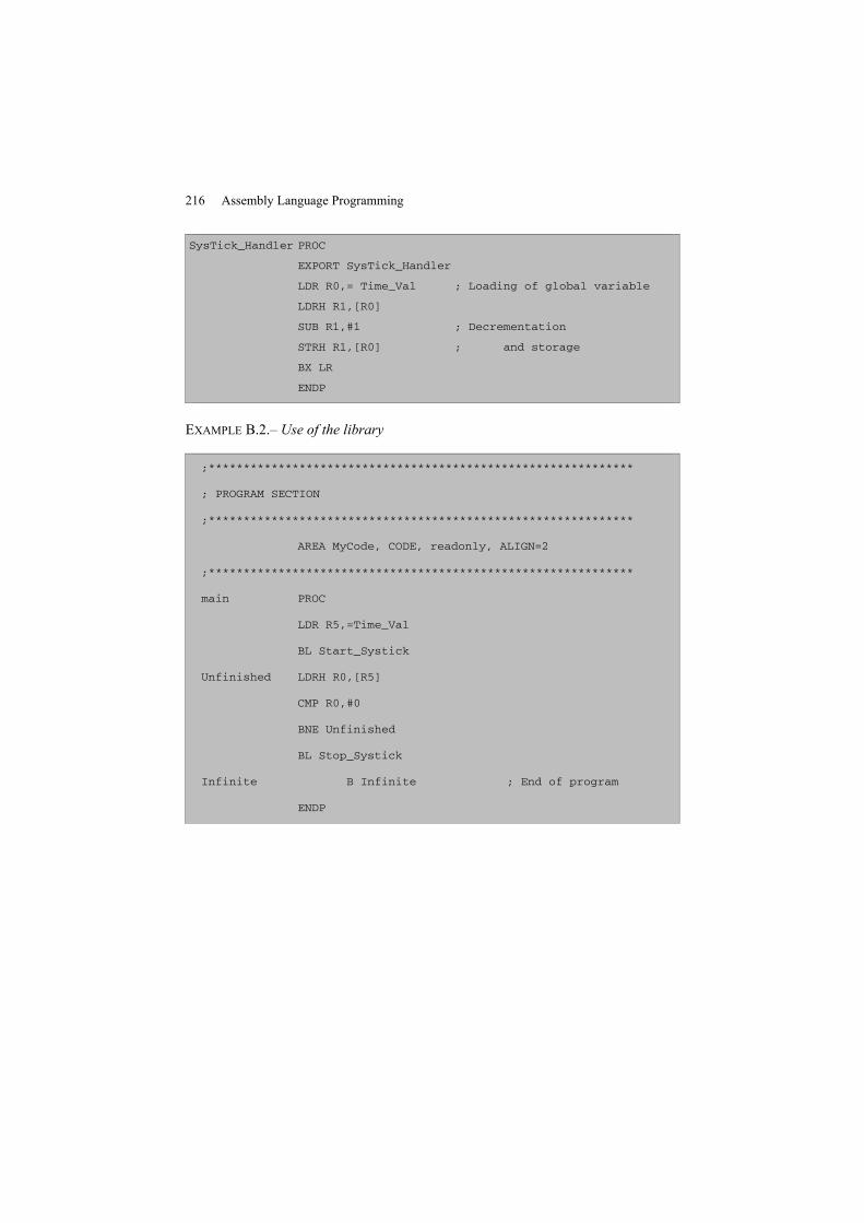
216 Assembly Language Programming
SysTick_Handler PROC
EXPORT SysTick_Handler
LDR R0,= Time_Val ; Loading of global variable
LDRH R1,[R0]
SUB R1,#1 ; Decrementation
STRH R1,[R0] ; and storage
BX LR
ENDP
EXAMPLE B.2.– Use of the library
;*************************************************************
; PROGRAM SECTION
;*************************************************************
AREA MyCode, CODE, readonly, ALIGN=2
;*************************************************************
main PROC
LDR R5,=Time_Val
BL Start_Systick
Unfinished LDRH R0,[R5]
CMP R0,#0
BNE Unfinished
BL Stop_Systick
Infinite B Infinite ; End of program
ENDP
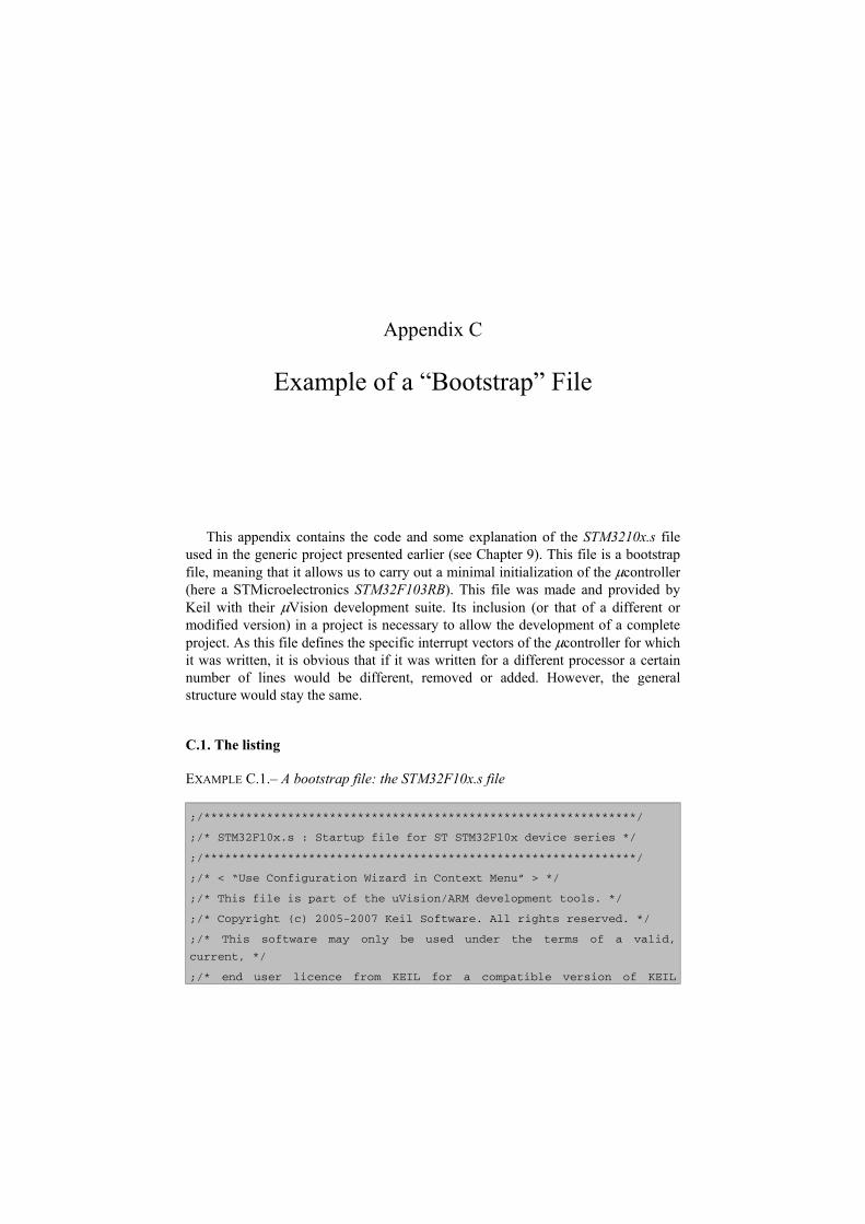
Appendix C
Example of a “Bootstrap” File
This appendix contains the code and some explanation of the STM3210x.s fileused in the generic project presented earlier (see Chapter 9). This file is a bootstrapfile, meaning that it allows us to carry out a minimal initialization of the μcontroller(here a STMicroelectronics STM32F103RB). This file was made and provided byKeil with their μVision development suite. Its inclusion (or that of a different ormodified version) in a project is necessary to allow the development of a completeproject. As this file defines the specific interrupt vectors of the μcontroller for whichit was written, it is obvious that if it was written for a different processor a certainnumber of lines would be different, removed or added. However, the generalstructure would stay the same.
C.1. The listing
EXAMPLE C.1.– A bootstrap file: the STM32F10x.s file
;/**************************************************************/
;/* STM32F10x.s : Startup file for ST STM32F10x device series */
;/**************************************************************/
;/* < “Use Configuration Wizard in Context Menu” > */
;/* This file is part of the uVision/ARM development tools. */
;/* Copyright (c) 2005-2007 Keil Software. All rights reserved. */
;/* This software may only be used under the terms of a valid,
current, */
;/* end user licence from KEIL for a compatible version of KEIL
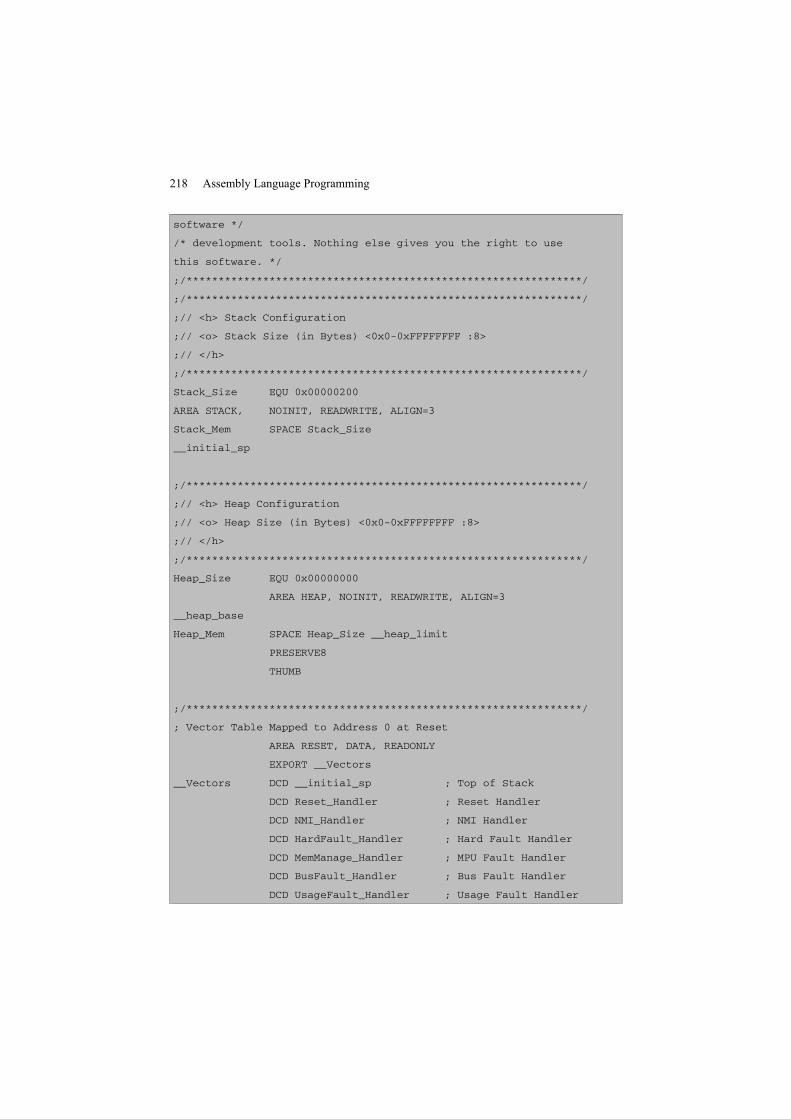
218 Assembly Language Programming
software */
/* development tools. Nothing else gives you the right to use
this software. */
;/**************************************************************/
;/**************************************************************/
;// <h> Stack Configuration
;// <o> Stack Size (in Bytes) <0x0-0xFFFFFFFF :8>
;// </h>
;/**************************************************************/
Stack_Size EQU 0x00000200
AREA STACK, NOINIT, READWRITE, ALIGN=3
Stack_Mem SPACE Stack_Size
__initial_sp
;/**************************************************************/
;// <h> Heap Configuration
;// <o> Heap Size (in Bytes) <0x0-0xFFFFFFFF :8>
;// </h>
;/**************************************************************/
Heap_Size EQU 0x00000000
AREA HEAP, NOINIT, READWRITE, ALIGN=3
__heap_base
Heap_Mem SPACE Heap_Size __heap_limit
PRESERVE8
THUMB
;/**************************************************************/
; Vector Table Mapped to Address 0 at Reset
AREA RESET, DATA, READONLY
EXPORT __Vectors
__Vectors DCD __initial_sp ; Top of Stack
DCD Reset_Handler ; Reset Handler
DCD NMI_Handler ; NMI Handler
DCD HardFault_Handler ; Hard Fault Handler
DCD MemManage_Handler ; MPU Fault Handler
DCD BusFault_Handler ; Bus Fault Handler
DCD UsageFault_Handler ; Usage Fault Handler
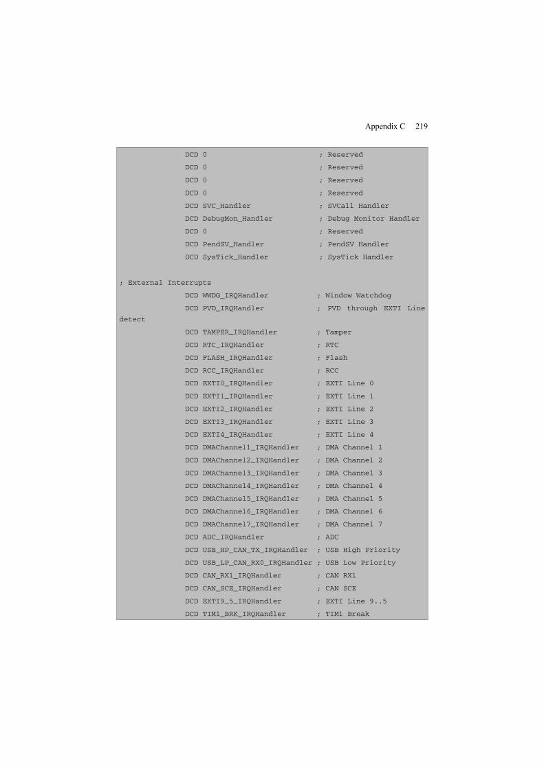
Appendix C 219
DCD 0 ; Reserved
DCD 0 ; Reserved
DCD 0 ; Reserved
DCD 0 ; Reserved
DCD SVC_Handler ; SVCall Handler
DCD DebugMon_Handler ; Debug Monitor Handler
DCD 0 ; Reserved
DCD PendSV_Handler ; PendSV Handler
DCD SysTick_Handler ; SysTick Handler
; External Interrupts
DCD WWDG_IRQHandler ; Window Watchdog
DCD PVD_IRQHandler ; PVD through EXTI Line
detect
DCD TAMPER_IRQHandler ; Tamper
DCD RTC_IRQHandler ; RTC
DCD FLASH_IRQHandler ; Flash
DCD RCC_IRQHandler ; RCC
DCD EXTI0_IRQHandler ; EXTI Line 0
DCD EXTI1_IRQHandler ; EXTI Line 1
DCD EXTI2_IRQHandler ; EXTI Line 2
DCD EXTI3_IRQHandler ; EXTI Line 3
DCD EXTI4_IRQHandler ; EXTI Line 4
DCD DMAChannel1_IRQHandler ; DMA Channel 1
DCD DMAChannel2_IRQHandler ; DMA Channel 2
DCD DMAChannel3_IRQHandler ; DMA Channel 3
DCD DMAChannel4_IRQHandler ; DMA Channel 4
DCD DMAChannel5_IRQHandler ; DMA Channel 5
DCD DMAChannel6_IRQHandler ; DMA Channel 6
DCD DMAChannel7_IRQHandler ; DMA Channel 7
DCD ADC_IRQHandler ; ADC
DCD USB_HP_CAN_TX_IRQHandler ; USB High Priority
DCD USB_LP_CAN_RX0_IRQHandler ; USB Low Priority
DCD CAN_RX1_IRQHandler ; CAN RX1
DCD CAN_SCE_IRQHandler ; CAN SCE
DCD EXTI9_5_IRQHandler ; EXTI Line 9..5
DCD TIM1_BRK_IRQHandler ; TIM1 Break
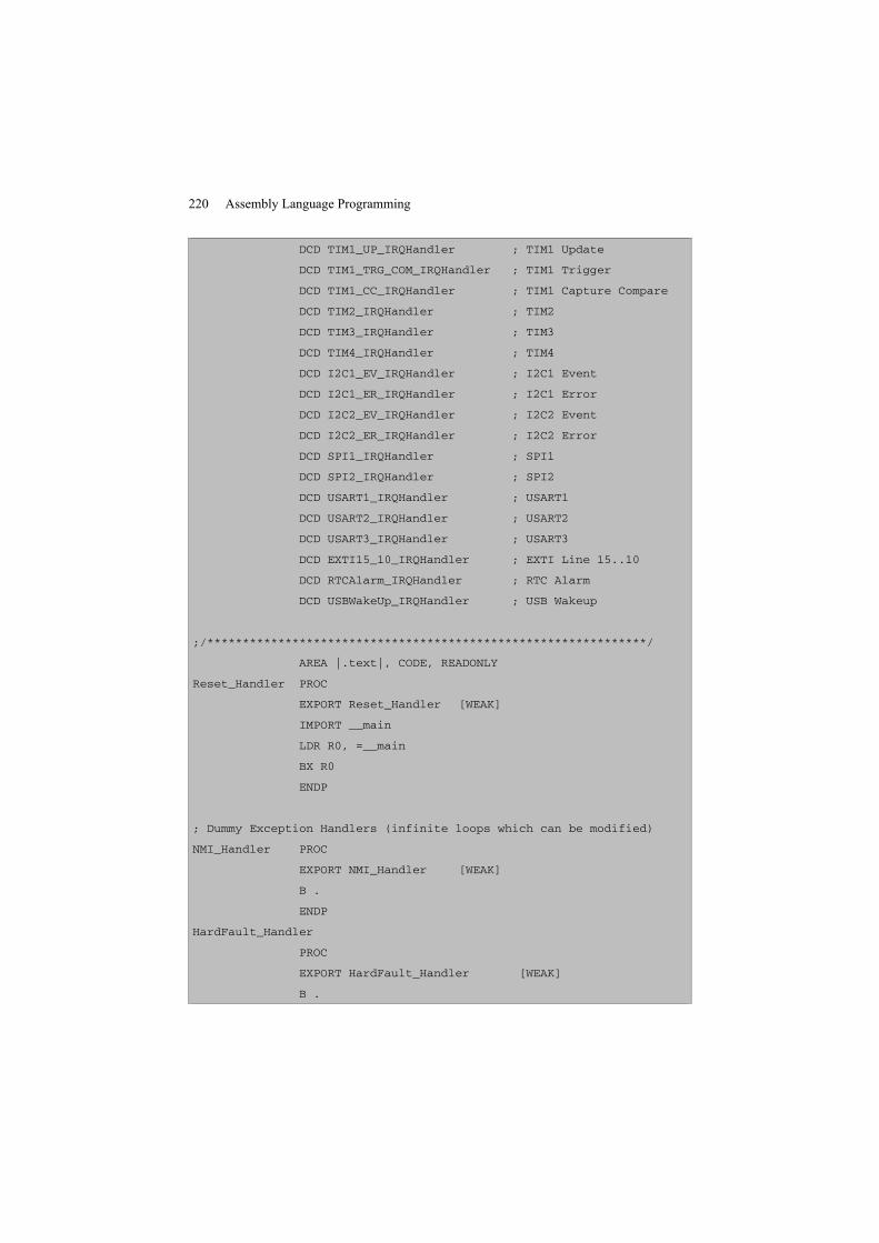
220 Assembly Language Programming
DCD TIM1_UP_IRQHandler ; TIM1 Update
DCD TIM1_TRG_COM_IRQHandler ; TIM1 Trigger
DCD TIM1_CC_IRQHandler ; TIM1 Capture Compare
DCD TIM2_IRQHandler ; TIM2
DCD TIM3_IRQHandler ; TIM3
DCD TIM4_IRQHandler ; TIM4
DCD I2C1_EV_IRQHandler ; I2C1 Event
DCD I2C1_ER_IRQHandler ; I2C1 Error
DCD I2C2_EV_IRQHandler ; I2C2 Event
DCD I2C2_ER_IRQHandler ; I2C2 Error
DCD SPI1_IRQHandler ; SPI1
DCD SPI2_IRQHandler ; SPI2
DCD USART1_IRQHandler ; USART1
DCD USART2_IRQHandler ; USART2
DCD USART3_IRQHandler ; USART3
DCD EXTI15_10_IRQHandler ; EXTI Line 15..10
DCD RTCAlarm_IRQHandler ; RTC Alarm
DCD USBWakeUp_IRQHandler ; USB Wakeup
;/**************************************************************/
AREA |.text|, CODE, READONLY
Reset_Handler PROC
EXPORT Reset_Handler [WEAK]
IMPORT __main
LDR R0, =__main
BX R0
ENDP
; Dummy Exception Handlers (infinite loops which can be modified)
NMI_Handler PROC
EXPORT NMI_Handler [WEAK]
B .
ENDP
HardFault_Handler
PROC
EXPORT HardFault_Handler [WEAK]
B .
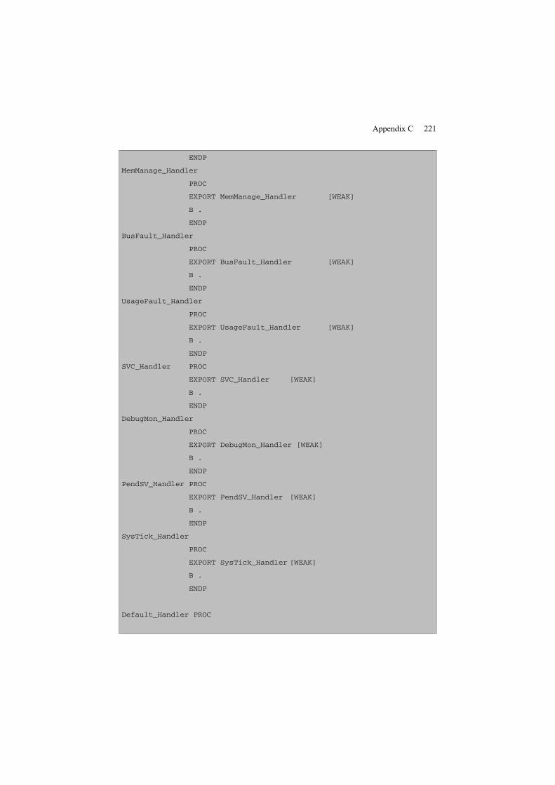
Appendix C 221
ENDP
MemManage_Handler
PROC
EXPORT MemManage_Handler [WEAK]
B .
ENDP
BusFault_Handler
PROC
EXPORT BusFault_Handler [WEAK]
B .
ENDP
UsageFault_Handler
PROC
EXPORT UsageFault_Handler [WEAK]
B .
ENDP
SVC_Handler PROC
EXPORT SVC_Handler [WEAK]
B .
ENDP
DebugMon_Handler
PROC
EXPORT DebugMon_Handler [WEAK]
B .
ENDP
PendSV_Handler PROC
EXPORT PendSV_Handler [WEAK]
B .
ENDP
SysTick_Handler
PROC
EXPORT SysTick_Handler [WEAK]
B .
ENDP
Default_Handler PROC
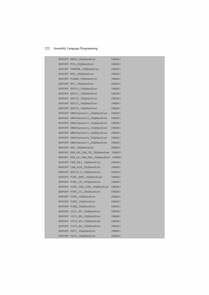
222 Assembly Language Programming
EXPORT WWDG_IRQHandler [WEAK]
EXPORT PVD_IRQHandler [WEAK]
EXPORT TAMPER_IRQHandler [WEAK]
EXPORT RTC_IRQHandler [WEAK]
EXPORT FLASH_IRQHandler [WEAK]
EXPORT RCC_IRQHandler [WEAK]
EXPORT EXTI0_IRQHandler [WEAK]
EXPORT EXTI1_IRQHandler [WEAK]
EXPORT EXTI2_IRQHandler [WEAK]
EXPORT EXTI3_IRQHandler [WEAK]
EXPORT EXTI4_IRQHandler [WEAK]
EXPORT DMAChannel1_IRQHandler [WEAK]
EXPORT DMAChannel2_IRQHandler [WEAK]
EXPORT DMAChannel3_IRQHandler [WEAK]
EXPORT DMAChannel4_IRQHandler [WEAK]
EXPORT DMAChannel5_IRQHandler [WEAK]
EXPORT DMAChannel6_IRQHandler [WEAK]
EXPORT DMAChannel7_IRQHandler [WEAK]
EXPORT ADC_IRQHandler [WEAK]
EXPORT USB_HP_CAN_TX_IRQHandler [WEAK]
EXPORT USB_LP_CAN_RX0_IRQHandler [WEAK]
EXPORT CAN_RX1_IRQHandler [WEAK]
EXPORT CAN_SCE_IRQHandler [WEAK]
EXPORT EXTI9_5_IRQHandler [WEAK]
EXPORT TIM1_BRK_IRQHandler [WEAK]
EXPORT TIM1_UP_IRQHandler [WEAK]
EXPORT TIM1_TRG_COM_IRQHandler [WEAK]
EXPORT TIM1_CC_IRQHandler [WEAK]
EXPORT TIM2_IRQHandler [WEAK]
EXPORT TIM3_IRQHandler [WEAK]
EXPORT TIM4_IRQHandler [WEAK]
EXPORT I2C1_EV_IRQHandler [WEAK]
EXPORT I2C1_ER_IRQHandler [WEAK]
EXPORT I2C2_EV_IRQHandler [WEAK]
EXPORT I2C2_ER_IRQHandler [WEAK]
EXPORT SPI1_IRQHandler [WEAK]
EXPORT SPI2_IRQHandler [WEAK]
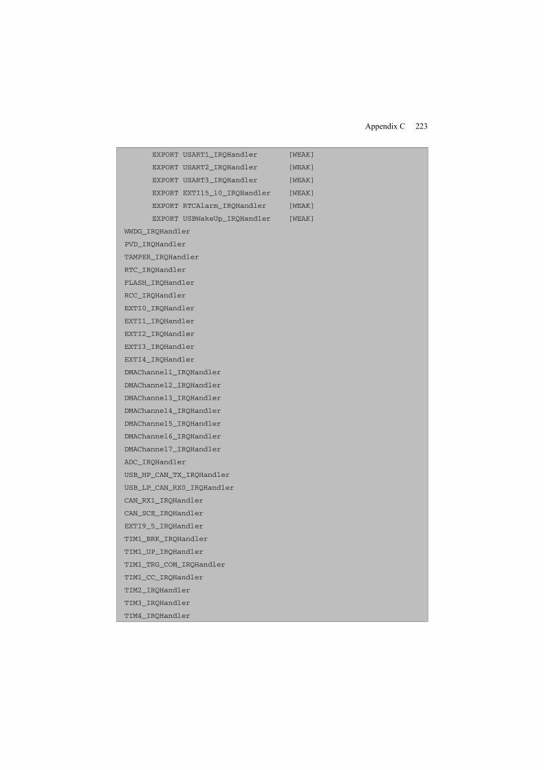
Appendix C 223
EXPORT USART1_IRQHandler [WEAK]
EXPORT USART2_IRQHandler [WEAK]
EXPORT USART3_IRQHandler [WEAK]
EXPORT EXTI15_10_IRQHandler [WEAK]
EXPORT RTCAlarm_IRQHandler [WEAK]
EXPORT USBWakeUp_IRQHandler [WEAK]
WWDG_IRQHandler
PVD_IRQHandler
TAMPER_IRQHandler
RTC_IRQHandler
FLASH_IRQHandler
RCC_IRQHandler
EXTI0_IRQHandler
EXTI1_IRQHandler
EXTI2_IRQHandler
EXTI3_IRQHandler
EXTI4_IRQHandler
DMAChannel1_IRQHandler
DMAChannel2_IRQHandler
DMAChannel3_IRQHandler
DMAChannel4_IRQHandler
DMAChannel5_IRQHandler
DMAChannel6_IRQHandler
DMAChannel7_IRQHandler
ADC_IRQHandler
USB_HP_CAN_TX_IRQHandler
USB_LP_CAN_RX0_IRQHandler
CAN_RX1_IRQHandler
CAN_SCE_IRQHandler
EXTI9_5_IRQHandler
TIM1_BRK_IRQHandler
TIM1_UP_IRQHandler
TIM1_TRG_COM_IRQHandler
TIM1_CC_IRQHandler
TIM2_IRQHandler
TIM3_IRQHandler
TIM4_IRQHandler
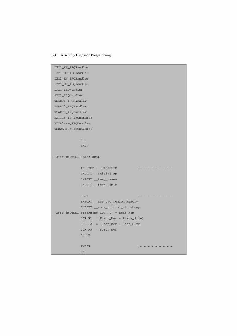
224 Assembly Language Programming
I2C1_EV_IRQHandler
I2C1_ER_IRQHandler
I2C2_EV_IRQHandler
I2C2_ER_IRQHandler
SPI1_IRQHandler
SPI2_IRQHandler
USART1_IRQHandler
USART2_IRQHandler
USART3_IRQHandler
EXTI15_10_IRQHandler
RTCAlarm_IRQHandler
USBWakeUp_IRQHandler
B .
ENDP
; User Initial Stack Heap
IF :DEF :__MICROLIB ;– – – – – – – – –
EXPORT __initial_sp
EXPORT __heap_basev
EXPORT __heap_limit
ELSE ;– – – – – – – – –
IMPORT __use_two_region_memory
EXPORT __user_initial_stackheap
__user_initial_stackheap LDR R0, = Heap_Mem
LDR R1, =(Stack_Mem + Stack_Size)
LDR R2, = (Heap_Mem + Heap_Size)
LDR R3, = Stack_Mem
BX LR
ENDIF ;– – – – – – – – –
END
Appendix C 225
C.2. Important points
This listing requires some explanation, even if its blind use causes no majorproblems:
– In this version, the system stack (Stack_Mem) is 512 bytes in dimension. Thetop of the stack is marked with __initial_stack, which is the first address followingthe reserved zone as the system stack is pre-decrementation.
– A heap (Heap_Mem) is reserved in the same way as the reservation for thesystem stack. This reservation is for the use of the C compiler (standard library). It isinteresting to note, however, that in this case the reservation is completely fictitioussince the size (Heap_Size) reserved is zero. It is only there to avoid causingresolution errors during link editing.
– The interrupt vector table corresponds to a set of words initialized with theaddresses of exception processing routines that exist lower in the module. It starts bystoring the highest address of the previously declared stack. The STM32 used in thisproject is built around 43 interrupt vectors.
– The interrupt handler set is limited to a single B., or infinite loop. This moduleis therefore only a simple skeleton for the development of more adapted routines.These routines are really wells: if an exception is launched and nothing but theskeleton has been developed, it is impossible to escape other than by Reset.
– The external exceptions (which correspond to interrupts) are all grouped in thesame routine. This routine has some 43 different names. All of these names areWEAK (another statement will be given priority over them) and exported to bevisible from other modules.
– The Reset handler is the only one that contains a little code. It simply calls the__main routine, which is the entry point to the MicroLib library. This same routinewill end it by a jump to the label main, which is the entry point of the project. TheMicroLib source is not directly accessible; but by opening a disassembly window indebug mode, it is possible to view its content.
– At the end of the listing are lines that allow the export of the addresses of thestack and heap, in particular for the MicroLib library if it is included in the project.Otherwise (ELSE alternative), it is assumed that the standard library is used, inwhich case the __user_initial_stackheap procedure is necessary for its correctrunning and for where it exports to. This procedure fills the R0 to R3 registers withthe addresses of reservation delimitations from the stack and the heap.

Appendix D
The GNU Assembler
The set of examples presented in this work are written for the ARM-MDK(Microcontroller Development Kit). Another compiler/assembler/link editor trio,however, is currently used to construct such projects. This is the compilation chainGNU1-GCC (GNU Compiler Connection), which as its name suggests comes fromthe world of free and cooperative software. This appendix is based specifically onthe Sourcery G++ Lite tools for ARM EABI (Embedded-Application BinaryInterface). This precision is important insofar as, although the tools are designed tobe generic, they still have specificities and peculiarities that make them somewhatmore difficult to understand and use. As an example to illustrate this, take theofficial documentation for the Sourcery G++ assembler. This documentation is 328pages long, and 202 pages (Chapter 9) are dedicated to the characteristics unique toeach processor. Despite the peculiarities, it is interesting to draw on the commonpoints between the different GNU compilers/assemblers/link editors in order to beable to develop programs with different tools and/or processors.
The ARM-MDK and GNU-GCC projects are not cross-compatible, which mightseem surprising since the processor and thus the instruction set are very similar. Thetwo major differences are found in the syntax used for the directives (for theassembler) and in the way of describing the memory (for the link editor). We shouldnote that the use of the GNU GCC tool is still possible in the Keil μVisionenvironment, which is interesting as this environment is completely functional in itsfree trial version and so it is possible to use the μcontroller emulator that it offers.
1 GNU is a Unix-like computer operating system and corresponds to the recursiveacronym “GNU is Not Unix”
228 Assembly Language Programming
In the first part of this appendix, we will list the main directives necessary todevelop a project, for instance that which was presented in Chapter 3. In section D.2we will give an example of a program written with these syntax rules that aims tomake up for the absence of the MicroLib library. We will not develop the aspectstied to the linker, and especially the memory description file, here due to thecomplexity of their construction. The Sourcery G++ suite for ARM EABI issupplied with the typical files (generic.ld for example) from which it is possible tostart.
D.1. GNU directive
In the GNU world, the set of instructions that we want to give to the compiler orassembly (directives) will be introduced by a keyword prefixed by a “.” (dot). Thevast majority of directives that we have explored (see Chapter 3) have their directequivalents in this version of the assembler, but there are a certain number ofadditions, differences and subtleties that we must carefully understand when weswitch from the ARM universe to the GNU universe.
D.1.1. Generalities
These are not strictly the directives mentioned but the following syntactic rulesmust be respected in order to produce code that is acceptable to the assembler:
– the commentaries are, as is usual in C, the set of characters between thedelimiters ‘/*’ and ‘*/’. The user has a second chance to insert a comment byinserting an ‘@’. The rest of the line (until carriage return) will then be ignored.This second syntax is inevitably not very readable;
– symbols are made up of several “letter” characters (upper or lower case),“number” characters (with the exception of the first character) and the two specialcharacters ‘.’ and ‘_’. Please note that the ‘$’ character, which is allowed in otherprocessors, cannot be used here because (like #) it indicates the start of animmediate value;
– a label is a symbol followed by a ‘:’;
– there are no differences when giving the expression of a numerical value otherthan for expression in any numerical base. Only bases 10, 16 and binary are allowed.For binary numbers, the value must be prefixed with 0b. For example, theinstructionMOV R0, #0b100 would load the value 4 in R0.
Appendix D 229
D.1.2.Memory management
There is not a single directive to create sections. There are three directives thatallow us to carry out openings (closings happen automatically with the opening of anew section). These are identified by the type of section that they create:
– .text lets us open a section of code;
– .data lets us open a section of initialized data;
– .bss lets us open a section of data initially set to zero.
These directives do not support certain options, unlike the ARM directive AREA.However, it is possible to add other directives to the section opening suite to specifyspecific properties:
– .align n allows us to impose an alignment on the instruction or datum thatfollows this directive. The alignment will be to an address divisible by 2n;
– .ltorg allows us to specify that the contents of the Literal Pool must be placedin this section (which must be of the .text type).
D.1.3.Management of variables
The different directives that follow allow us to make various reservations. Do notforget that the symbols that will correspond to these reservations must, as for thelabels, be followed by ‘:’:
– .ascii “string...” makes a reservation of as many bytes as there are charactersin the chain following this directive. Note that a .asciiz version exists and is set at 0at the end of the chain;
– .byte exp1{,exp2}{,...} reserves a byte initialized by exp. There are as manyreservations as expressions;
– .equ symbol, expression acts as a find (symbol)/replace (expression) in thecurrent module. This directive therefore allows us to define constants;
– .fill repeat {,size}{,value} allows us to create repeat copies of the value valuecoded on size bytes. If value is not defined, the value will be zero. If size is notspecified, the default size will be one byte;
– .hword exp1{,exp2}{,...} is equivalent to .byte for 16-bit reservations (a half-word);
230 Assembly Language Programming
– .space size {,fill} reserves size bytes filled with fill (less than 255). Theabsence of fill leads to initialization at 0;
– .word exp1 {,exp2}{,...} is equivalent to .byte for 32-bit reservations.
D.1.4. Conditional assembly
The following directives allow us to carry out conditional assembly (see section3.5.2):
– .if expression means that the lines that follow will be included in the section ifexpression is not false;
– .endif marks the end of the conditional part;
– .else allows us to include an alternative composed with .if.
D.1.5.Miscellaneous
There are other directives that can be necessary or useful:
– A module ends with .end. The assembler ignores the lines that follow thisdirective.
– The directive .type allows us to give additional information on a symbol. Thisinformation can be particularly useful with the use of a symbolic debugger. Themost common use is .type symbol,%function to indicate that the label symbolcorresponds to a procedure entry.
– There are no specific directives for indicating the importation of a symbol (seesection 9.1.5). It is enough, in the module where the insertion of the directive .globalsymbol is declared, that symbol is shared with other symbols of the same nameduring link editing. This directive carries out the exportation of a symbol.
– .weak name marks the symbol name as weak in the symbol table. This meansthat another definition of the symbol will have a higher priority than this typeddeclaration.
– .size name, expression associates a size (expression) with a symbol (name).The dimension can be the result of a calculation, such as the difference between twosymbols. This directive is typically used to calculate, for example, how much spacea function takes up. For example, .size Dim . – Deb_func will assign the dimensioncorresponding to the difference between the current address (.) and the address ofthe symbol Deb_func to the symbol Dim.
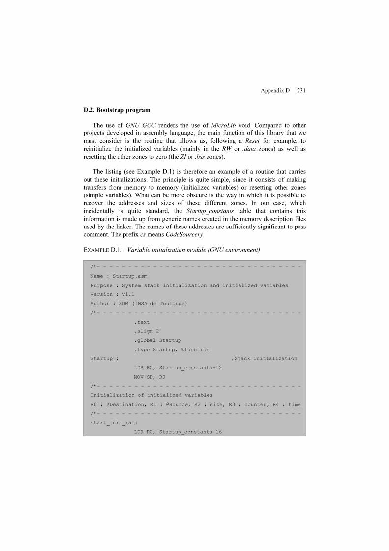
Appendix D 231
D.2. Bootstrap program
The use of GNU GCC renders the use of MicroLib void. Compared to other projects developed in assembly language, the main function of this library that we must consider is the routine that allows us, following a Reset for example, to reinitialize the initialized variables (mainly in the RW or .data zones) as well as resetting the other zones to zero (the ZI or .bss zones).
The listing (see Example D.1) is therefore an example of a routine that carries out these initializations. The principle is quite simple, since it consists of making transfers from memory to memory (initialized variables) or resetting other zones (simple variables). What can be more obscure is the way in which it is possible to recover the addresses and sizes of these different zones. In our case, which incidentally is quite standard, the Startup_constants table that contains this information is made up from generic names created in the memory description files used by the linker. The names of these addresses are sufficiently significant to pass comment. The prefix cs means CodeSourcery.
EXAMPLE D.1.− Variable initialization module (GNU environment)
/*– – – – – – – – – – – – – – – – – – – – – – – – – – – – – – – – –
Name : Startup.asm
Purpose : System stack initialization and initialized variables
Version : V1.1
Author : SDM (INSA de Toulouse)
/*– – – – – – – – – – – – – – – – – – – – – – – – – – – – – – – – –
.text
.align 2
.global Startup
.type Startup, %function
Startup : ;Stack initialization
LDR R0, Startup_constants+12
MOV SP, R0
/*– – – – – – – – – – – – – – – – – – – – – – – – – – – – – – – – –
Initialization of initialized variables
R0 : @Destination, R1 : @Source, R2 : size, R3 : counter, R4 : time
/*– – – – – – – – – – – – – – – – – – – – – – – – – – – – – – – – –
start_init_ram:
LDR R0, Startup_constants+16
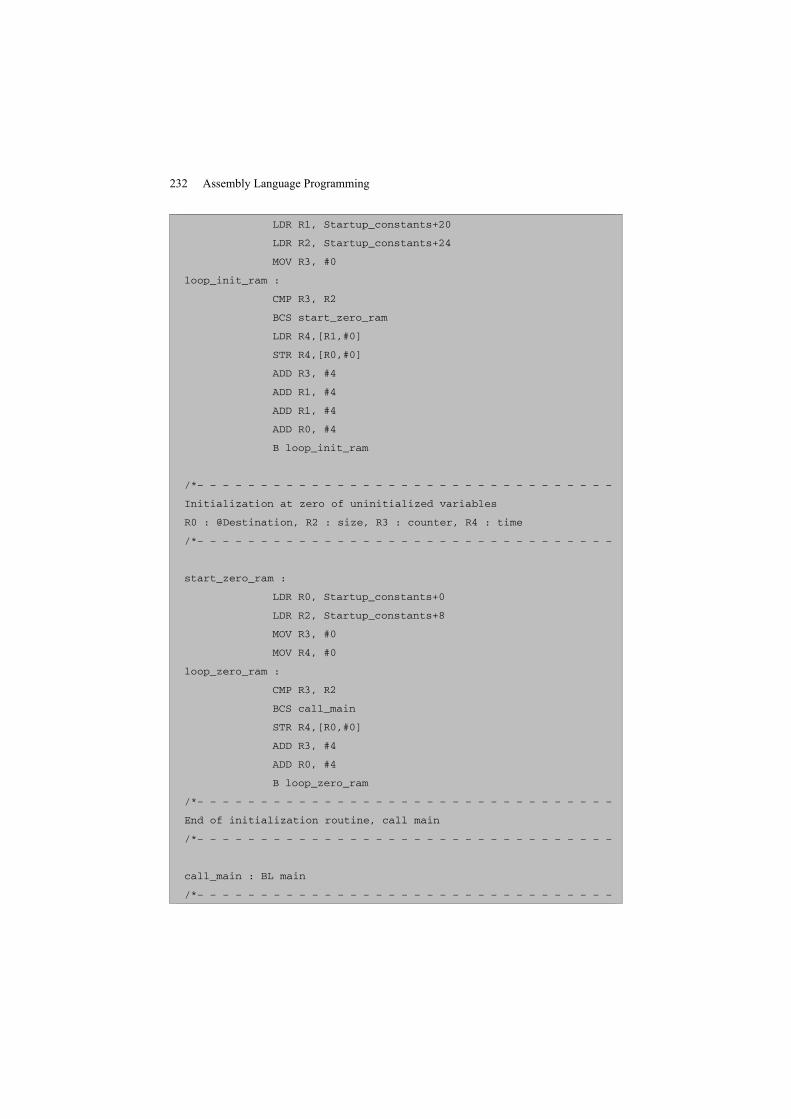
232 Assembly Language Programming
LDR R1, Startup_constants+20
LDR R2, Startup_constants+24
MOV R3, #0
loop_init_ram :
CMP R3, R2
BCS start_zero_ram
LDR R4,[R1,#0]
STR R4,[R0,#0]
ADD R3, #4
ADD R1, #4
ADD R1, #4
ADD R0, #4
B loop_init_ram
/*– – – – – – – – – – – – – – – – – – – – – – – – – – – – – – – – –
Initialization at zero of uninitialized variables
R0 : @Destination, R2 : size, R3 : counter, R4 : time
/*– – – – – – – – – – – – – – – – – – – – – – – – – – – – – – – – –
start_zero_ram :
LDR R0, Startup_constants+0
LDR R2, Startup_constants+8
MOV R3, #0
MOV R4, #0
loop_zero_ram :
CMP R3, R2
BCS call_main
STR R4,[R0,#0]
ADD R3, #4
ADD R0, #4
B loop_zero_ram
/*– – – – – – – – – – – – – – – – – – – – – – – – – – – – – – – – –
End of initialization routine, call main
/*– – – – – – – – – – – – – – – – – – – – – – – – – – – – – – – – –
call_main : BL main
/*– – – – – – – – – – – – – – – – – – – – – – – – – – – – – – – – –
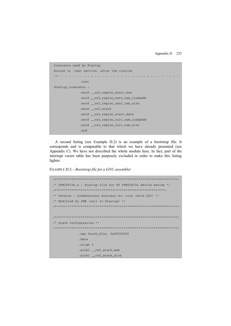
Appendix D 233
Constants used by Startup
Stored in .text section, after the routine
/*– – – – – – – – – – – – – – – – – – – – – – – – – – – – – – – – –
.text
Startup_constants :
.word __cs3_region_start_bss
.word __cs3_region_zero_ram_loadaddr
.word __cs3_region_zero_ram_size
.word __cs3_stack
.word __cs3_region_start_data
.word __cs3_region_init_ram_loadaddr
.word __cs3_region_init_ram_size
.end
A second listing (see Example D.2) is an example of a bootstrap file. Itcorresponds and is comparable to that which we have already presented (seeAppendix C). We have not described the whole module here. In fact, part of theinterrupt vector table has been purposely excluded in order to make this listinglighter.
EXAMPLE D.2.– Bootstrap file for a GNU assembler
/******************************************************************/
/* STM32F10x.s : Startup file for ST STM32F10x device series */
/***********************************************************/
/* Version : CodeSourcery Sourcery G++ Lite (with CS3) */
/* Modified by SDM (call to Startup) */
/******************************************************************/
/******************************************************************/
/* Stack Configuration */
/******************************************************************/
.equ Stack_Size, 0x00000200
.data
.align 3
.globl __cs3_stack_mem
.globl __cs3_stack_size
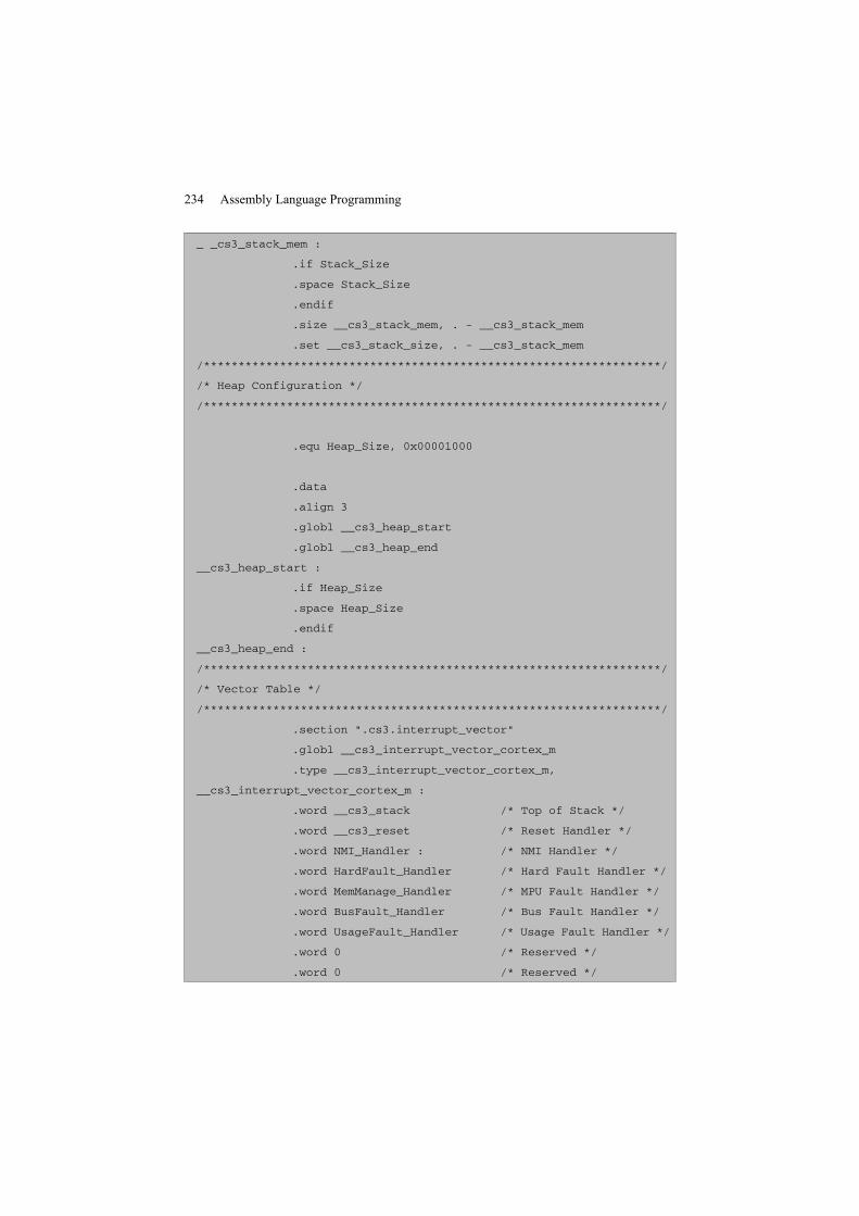
234 Assembly Language Programming
_ _cs3_stack_mem :
.if Stack_Size
.space Stack_Size
.endif
.size __cs3_stack_mem, . - __cs3_stack_mem
.set __cs3_stack_size, . - __cs3_stack_mem
/******************************************************************/
/* Heap Configuration */
/******************************************************************/
.equ Heap_Size, 0x00001000
.data
.align 3
.globl __cs3_heap_start
.globl __cs3_heap_end
__cs3_heap_start :
.if Heap_Size
.space Heap_Size
.endif
__cs3_heap_end :
/******************************************************************/
/* Vector Table */
/******************************************************************/
.section ".cs3.interrupt_vector"
.globl __cs3_interrupt_vector_cortex_m
.type __cs3_interrupt_vector_cortex_m,
__cs3_interrupt_vector_cortex_m :
.word __cs3_stack /* Top of Stack */
.word __cs3_reset /* Reset Handler */
.word NMI_Handler : /* NMI Handler */
.word HardFault_Handler /* Hard Fault Handler */
.word MemManage_Handler /* MPU Fault Handler */
.word BusFault_Handler /* Bus Fault Handler */
.word UsageFault_Handler /* Usage Fault Handler */
.word 0 /* Reserved */
.word 0 /* Reserved */
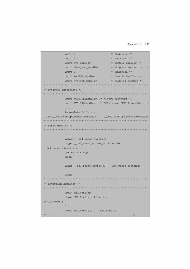
Appendix D 235
.word 0 /* Reserved */
.word 0 /* Reserved */
.word SVC_Handler /* SVCall Handler */
.word DebugMon_Handler /*Debug Monitor Handler */
.word 0 /* Reserved */
.word PendSV_Handler /* PendSV Handler */
.word SysTick_Handler /* SysTick Handler */
/******************************************************************/
/* External Interrupts */
/******************************************************************/
.word WWDG_IRQHandler /* Window Watchdog */
.word PVD_IRQHandler /* PVD through EXTI Line detect */
...
Incomplete Table....
.size __cs3_interrupt_vector_cortex_m, . - __cs3_interrupt_vector_cortex_m
/******************************************************************/
/* Reset Handler */
/******************************************************************/
.text
.globl __cs3_reset_cortex_m
.type __cs3_reset_cortex_m, %function
__cs3_reset_cortex_m :
LDR R0,=Startup
BX R0
.size __cs3_reset_cortex_m,.-__cs3_reset_cortex_m
.text
/******************************************************************/
/* Exception Handlers */
/******************************************************************/
.weak NMI_Handler
.type NMI_Handler, %function
NMI_Handler :
B .
.size NMI_Handler, . - NMI_Handler
/* – – – – – – – – – – – – – – – – – – – – – – – – – – – –*/
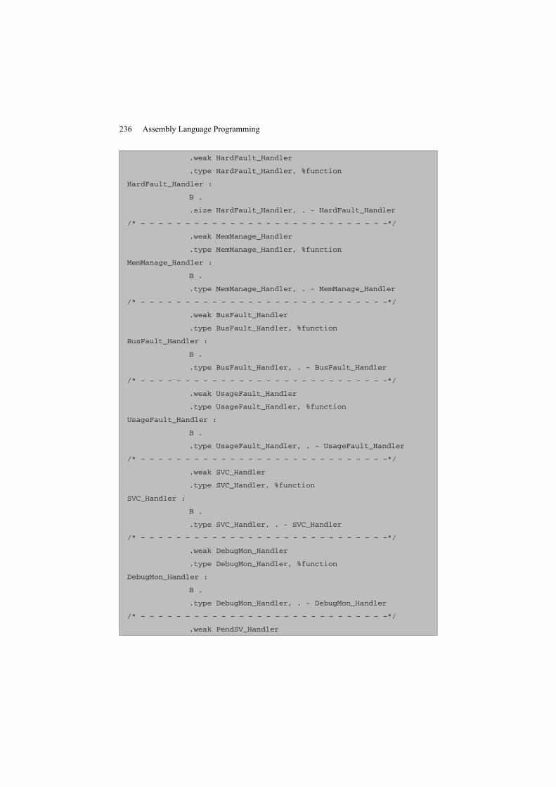
236 Assembly Language Programming
.weak HardFault_Handler
.type HardFault_Handler, %function
HardFault_Handler :
B .
.size HardFault_Handler, . - HardFault_Handler
/* – – – – – – – – – – – – – – – – – – – – – – – – – – – –*/
.weak MemManage_Handler
.type MemManage_Handler, %function
MemManage_Handler :
B .
.type MemManage_Handler, . - MemManage_Handler
/* – – – – – – – – – – – – – – – – – – – – – – – – – – – –*/
.weak BusFault_Handler
.type BusFault_Handler, %function
BusFault_Handler :
B .
.type BusFault_Handler, . - BusFault_Handler
/* – – – – – – – – – – – – – – – – – – – – – – – – – – – –*/
.weak UsageFault_Handler
.type UsageFault_Handler, %function
UsageFault_Handler :
B .
.type UsageFault_Handler, . - UsageFault_Handler
/* – – – – – – – – – – – – – – – – – – – – – – – – – – – –*/
.weak SVC_Handler
.type SVC_Handler, %function
SVC_Handler :
B .
.type SVC_Handler, . - SVC_Handler
/* – – – – – – – – – – – – – – – – – – – – – – – – – – – –*/
.weak DebugMon_Handler
.type DebugMon_Handler, %function
DebugMon_Handler :
B .
.type DebugMon_Handler, . - DebugMon_Handler
/* – – – – – – – – – – – – – – – – – – – – – – – – – – – –*/
.weak PendSV_Handler
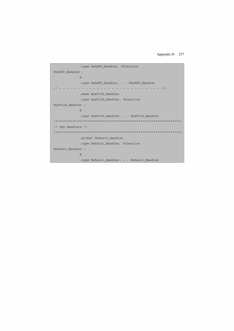
Appendix D 237
.type PendSV_Handler, %function
PendSV_Handler :
B .
.type PendSV_Handler, . - PendSV_Handler
/* – – – – – – – – – – – – – – – – – – – – – – – – – – – –*/
.weak SysTick_Handler
.type SysTick_Handler, %function
SysTick_Handler :
B .
.type SysTick_Handler, . - SysTick_Handler
/******************************************************************/
/* IRQ Handlers */
/******************************************************************/
.global Default_Handler
.type Default_Handler, %function
Default_Handler :
B .
.type Default_Handler, . - Default_Handler


Bibliography
[ARM 06a] ARM, ARMv7M Application Level Reference Manual, Arm Limited, Cambridge,2006.
[ARM 06b] ARM, ARMv7-M Architecture Reference Manual, Arm Limited, Cambridge,2006.
[ARM 06c] ARM, Cortex-M3 Technical Reference Manual, Arm Limited, Cambridge, 2006.
[ARM 10] ARM, RealView Compilation Tools − Assembler Guide, Arm Limited, Cambridge,2010.
[COD] CODESOURCERY, http://www.codesourcery.com.
[KEI] KEIL, http://www.keil.com.
[YIU 07] YIU J., The Definitive Guide to the Arm Cortex-M3, Elsevier, Amsterdam, 2007.

Index
Aaccess privilege, 16ADC, 52, 66, 201, 217,ADD, 30, 33, 49, 50, 52, 64, 67, 80,100, 129, 134, 137, 140, 143, 177,201, 231
addressing mode, 32, 47, 57, 59-61,100, 111, 114, 127, 134, 142
algorithm, 61, 87, 88, 91, 92, 94, 99,103, 109, 112
algorithmicalternative structures, 79, 89complete alternative, 90-93, 97iterative structures, 98multiple choice, 94simple alternative, 89-91, 93structures, 24, 44, 65, 76, 77, 79,
88ALIGN, 40, 56, 92, 96, 100, 101,121, 128, 214, 215, 216, 217
AND, 52, 65, 70, 77, 106-111, 157,201, 202, 207
annex pointer, 134, 137, 138, 143,144
AREA, 28, 33, 35, 41, 43, 56, 92, 96,100, 101, 121, 128, 136, 149, 176,177, 183, 214, 216, 217, 229
arguments, 2, 26, 37, 40, 104, 119,121-131, 133, 134, 136-138, 142,143, 146
ASCII table, 36ASR, 52, 70, 75, 201assembler, 1, 2, 25-28, 30, 32, 36-39,41, 43-45, 48-51, 53-55, 57- 59, 63,64, 78, 79, 88, 130, 133, 149, 151,173, 178-190, 197, 227, 228, 230,233
assemblyby pieces, 178directive, 9, 25, 111, 175,language, 1, 2, 4, 6, 9, 15, 17, 22,
24-30, 32, 35, 39, 41, 47, 58,61, 84, 87-89, 91, 94, 95, 101,103, 106-112, 120, 123, 125,136, 146, 175, 181, 182, 196,231
BBCC, 30, 33BFC, 70, 202BFI, 70, 202BIC, 70, 52, 202, 214bitbanding, 10shift, 64, 85
242 Assembly Language Programming
BL, 20, 21, 26, 35, 43, 44, 51, 56, 65,78, 92, 93, 95, 104, 105, 119-121,123-125, 129, 132, 134, 140, 176,183, 187, 202, 214, 216, 231
BLX, 78, 96, 97, 202bus(AHB), 5AHB-Lite, 5fault, 77, 153-156, 158, 161, 167,
170, 217, 233matrix, 5, 6PPB, 5
BX, 20, 21, 26, 35, 51, 56, 65, 77, 78,96, 105, 119-121, 124, 125, 129,132, 134, 137, 140, 143, 150, 155,157, 169, 177, 202, 214, 217, 233,
Ccarry C flag, 52, 70, 71CBNZ, 79, 202CBZ, 79, 202chained list, 143, 145CLRX, 85CLZ, 71, 202CM3CORE, 3, 15CMN, 76, 52, 202CMP, 52, 65, 66, 76, 79, 89, 90-93,95, 99, 100, 103-105, 107-111,121, 124, 125, 129, 132, 134, 157,202, 216, 231
codeaddress, 22, 198section, 57, 179, 180, 185, 189
COMMON, 40, 41, 136, 196compound condition, 106-111condition, 64-66, 76, 79, 88, 90, 98,99, 102, 106-109
conditionedassembly, 43jump, 65, 89, 102
CPD, 85CPS, 85cross development, 196
Ddatachain, 36, 38, 94, 95, 175, 185,193, 227, 229registration, 113section, 36, 47, 98, 136, 176, 179,
180, 185, 189, 196stack, 1, 18-20, 27, 40, 41, 51, 81,
83, 85, 115-117, 120, 126-131,133, 134, 136, 137, 139, 140,142-144, 148, 149, 157, 168,169, 182, 191, 217, 225, 231,233
structure, 32, 60, 61, 111, 114DCI, 41debug state, 16, 17debugger, 77, 174, 185, 197, 230debugging, 9, 85, 87, 158, 188-190,196, 198
disassembly, 25, 26, 54, 225doubleindirection, 97, 131pointing, 59, 131
DSB, 85DWT, 6dynamicallocation, 114data, 111, 127
E, F, GEOR, 52, 71, 202EQU, 30, 39, 40, 48, 128, 179, 214,217
ETM, 6EXPORT, 39, 45, 149, 150, 151, 176,177, 181-183, 214, 217
externalmodularity, 88, 175reference, 180
file, 2, 25, 27, 28, 39, 42, 44, 48, 88,173, 175, 178, 179, 182-185, 187-197, 217, 228, 233
Index 243
flag Q (saturation), 68, 69flash, 6, 9, 18, 189, 194, 197, 217FPB, 6GBLS, 43GET, 42
H, I, J, Khandler mode, 15, 16, 19, 168, 169heap, 40, 126-128, 136, 217, 225, 233identifier, 26, 29immediate operand, 47, 53-55, 63, 73IMPORT, 39, 45, 150, 176, 177, 180-183, 217
indirectaddressing with displacement, 60addressing with index, 112
initialized variable, 37, 39, 231instruction, 1-3, 6, 9, 16, 18-27, 29-
32, 34, 35, 38, 44, 47-55, 57-61,63-71, 73, 75-85, 87-89, 93, 95-97, 100, 105, 106, 119, 120, 123,131, 134, 137, 138, 140, 147, 149,153-158, 167-169, 173, 179, 182,185-187, 197, 201, 202, 227-229
pointer, 20, 21, 35, 51, 54, 78, 81,119, 149, 167-169
internal modularity, 88, 178interrupt, 4, 9, 15, 18, 23, 82, 86,
147-150, 152, 158-162, 166, 167,169, 171, 175, 181, 188, 192, 197,209-214, 217, 225, 233
vector table, 152, 181, 188, 192,213, 225, 233
ISB, 85IT, 23, 24, 64, 65, 79, 88, 106, 131,170, 202
ITM, 6JTAG, 6, 197, 198KEEP, 42, 180
Llabel, 26, 29, 30, 34, 36, 40-43, 45,48, 57, 75, 78, 79, 81, 83, 88, 89,96, 100, 106, 186, 187, 192, 193,201-203, 225, 228, 230
late-arriving, 169, 170LDM, 58, 78, 82, 84, 85, 131, 134,203
LDMDB, 82-84, 203LDR, 33, 34, 47, 54-58, 60, 61, 77,78, 81, 92, 93, 96, 97, 100-102,121, 124, 125, 128-132, 134, 137,140, 143, 146, 150, 157, 169, 176,177, 183, 186, 187, 203, 214, 216,217, 231, 233
LDRB, 33, 34, 58, 81, 101, 102, 104,105, 157, 163, 177
LDRBT, 58, 85LDRD, 58, 83, 203, 204LDREX, 85LDRH, 58-62, 81, 177, 214, 216LDRSB, 58, 81LDRSBT, 85LDRSH, 58, 81LIFO, 115, 117, 120, 126, 127literalexpression, 37, 38, 48pool, 55, 56
little endian, 10load/store architecture, 32, 104loader, 39, 174, 192, 196, 197local data, 1, 136, 137LSL, 52, 61, 71, 75, 80, 81, 96, 97,111, 163, 203, 204, 206, 207
LSR, 52, 71, 75, 79, 204LTORG, 39, 55-57
MMCR, 85MCRR, 86
244 Assembly Language Programming
memoryaddress, 9, 13, 21, 29, 32, 39, 97,147-149, 154, 170, 182, 192, 193management fault, 153
MLA, 67MLS, 67mnemonic, 2, 31, 35, 37, 58, 65, 72,78, 83, 84
modular programming, 119, 123, 178MOV, 2, 30, 33, 48, 53-55, 58, 75,95, 100-102, 121, 124, 125, 129,130, 132, 134, 137, 140, 143, 163,204, 228, 231
MOVT, 75, 204MPU, 4, 6, 217, 233MRC, 86MRRC, 86MRS, 24, 51, 75, 157, 170MSR, 24, 51, 76, 170, 204MUL, 67, 68, 177, 204MVN, 71, 204
N, O, Pnative development, 173, 196NEG, 72, 90, 101, 102, 204nested, 4, 15, 119, 120, 126, 127,133, 136, 140, 146, 148, 166, 169
NMI, 23, 147-149, 151, 153, 158,161, 170, 217, 233
NOP, 20, 21, 26, 32, 40, 56, 66, 182,204
numerical expression, 36NVIC, 4, 15, 148, 150, 153, 154, 156,159, 160-162, 165-167, 169-171
opcode, 18, 22, 50, 53, 157, 186, 187operand, 30, 32, 33, 39, 47, 52-54,58, 64, 68, 69, 187
ORN, 52, 72, 204ORR, 52, 72, 204, 214overlay, 196PENDSV, 158peripheral, 4, 5, 7-10, 154, 160
PLD, 86PLI, 86POP, 78, 84, 104, 105, 120, 121, 124,125, 129, 132-134, 137, 140, 143,169, 205, 214
PRESERVE8, 41, 217procedure arguments, 123, 137promotion, 58, 73, 81, 205PUSH, 19, 85, 104, 105, 120, 121,124, 125, 129, 132-134, 137, 140,143, 205, 214
RRAM, 9, 13, 18, 39, 188, 189, 195-197
RBIT, 72, 205registerAPSR, 23, 24, 75, 76base register, 57, 60-62, 64BasePri, 170, 171BFAR, 154CONTROL, 16, 18, 75, 76DHCSR, 17EPSR, 23, 24, 31, 75, 76, 155FaultMask, 170FAULTMASK, 18, 75, 76, 85general registers, 19, 23, 49, 51, 64,
123, 136high registers, 19ICER, 160ISER, 160ISPER, 161, 166, 171ISR, 23, 149low registers, 19LR, 18, 20, 21, 26, 35, 51, 56, 78,
84, 85, 96, 104, 105, 119-121,124, 125, 129, 132, 134, 137,140, 143, 155, 157, 168, 169,177, 194, 202, 214, 217
MSP (SP_Main), 19NVIC_IPR, 161, 162NVIC_SHCSR, 154

Index 245
NVIC_SHPR, 161, 162PC, 18, 19, 21, 22, 54, 55, 57, 58,
59, 75, 78-85, 104, 105, 119,120, 155, 157, 167-169, 186,197, 202, 203, 207, 214
PRIMASK, 18, 75, 76, 85R0 to R12, 18, 19, 49R13 or SP, 18, 19, 51, 148R14, 18-20, 51R15, 18, 21, 51, 82, 149UFSR, 153, 155, 156, 168
relocation table, 185-190REQUIRE8, 41reset, 4, 10, 16, 27, 143, 147-151,153, 158, 160, 161, 165, 167, 170,182, 185, 189, 192, 211, 212, 217,225, 231, 233
REV, 72, 73, 205REV16, 73, 205REVSH, 73, 205RN, 39, 49RO-data, 191, 192, 194ROR, 52, 73, 74, 205ROUT, 41, 42RRX, 52, 73RSB, 52, 67, 69, 72RW-data zone, 191
SSBC, 52, 68, 80SBFX, 73, 74, 205, 206SDIV, 68, 214SEV, 86simple executable, 175, 194SMLAL, 67, 68, 205SMULL, 68, 205SSAT, 23, 52, 68, 205stack, 1, 18-20, 27, 40, 41, 51, 81, 83,
85, 115-117, 120, 126-131, 133,134, 136, 137, 139, 140, 142-144,148, 149, 157, 168, 169, 182, 191,217, 225, 231, 233
pointer, 18, 27, 51, 81, 116, 117,120, 148, 149
STC, 86STM, 58, 82-85, 206STMDB, 82, 84, 206STR, 47, 57, 58, 60, 81, 82, 121, 124,125, 129, 132, 134, 137, 140, 143,206, 214, 231
STRB, 58, 81, 101, 102, 137, 143,163
STRBT, 85STRD, 58, 84, 206STREX, 85STRH, 58, 60, 81, 100, 137, 143,177, 214
STRSBT, 85SUB, 52, 67, 69, 80, 130, 134, 137,138, 140, 143, 206, 214
SVC, 86, 156-158, 161, 217, 233SVCall, 156, 157, 217, 233SWI, 86switch case, 94-98SXTB, 74, 206SXTH, 74, 206symbol, 21, 26, 27, 29, 30, 40-45, 48,
49, 64, 65, 112, 179, 180-182,185-190, 197, 228-230
table, 27, 43, 180, 181, 185-189,197, 230
system stack, 1, 2, 19, 27, 28, 41, 84,85, 104, 114, 117, 120, 125, 126,133-136, 148, 157, 168, 175, 191,197, 225, 231
SYSTICK, 212
T, Utail-chaining, 169, 170TBB, 80, 95, 96, 207TBH, 80, 95, 96, 207TEQ, 52, 77, 207thread mode, 15, 16, 19, 148, 168,169
246 Assembly Language Programming
thumb, 16, 17, 21, 23, 26, 31, 32, 49,50, 52, 77, 155, 187, 191
TPUI, 6trap, 82, 153-156, 158, 159TST, 52, 77, 93, 207typical table, 61UBFX, 73, 74, 207UDIV, 69, 177, 207UMLAL, 69, 207UMULL, 69usage fault, 39, 153, 155, 167, 168,217, 233
USAT, 23, 52, 69, 207user stack, 40, 127-131, 133, 136-138, 140, 142, 145, 146
UXTB, 74, 207UXTH, 74, 207
WWEAK, 150, 151, 176, 181-183, 217,225
WFE, 86WFI, 86YIELD, 86ZI-data zone, 192
~StormRG~