BioOne sees sustainable scholarly publishing as an inherently collaborative enterprise connecting authors nonprofit publishers academic institutions researchlibraries and research funders in the common goal of maximizing access to critical research

EVIDENCE OF RECENT RECRUITMENT IN THE OCEAN QUAHOGARCTICA ISLANDICA IN THE MID-ATLANTIC BIGHTAuthor(s) ERIC N POWELL and ROGER MANNSource Journal of Shellfish Research 24(2)517-530Published By National Shellfisheries AssociationDOI httpdxdoiorg1029830730-8000(2005)24[517EORRIT]20CO2URL httpwwwbiooneorgdoifull1029830730-800028200529245B5173AEORRIT5D20CO3B2

BioOne (wwwbiooneorg) is a nonprofit online aggregation of core research in the biological ecological andenvironmental sciences BioOne provides a sustainable online platform for over 170 journals and books publishedby nonprofit societies associations museums institutions and presses

Your use of this PDF the BioOne Web site and all posted and associated content indicates your acceptance ofBioOnersquos Terms of Use available at wwwbiooneorgpageterms_of_use

Usage of BioOne content is strictly limited to personal educational and non-commercial use Commercial inquiriesor rights and permissions requests should be directed to the individual publisher as copyright holder

EVIDENCE OF RECENT RECRUITMENT IN THE OCEAN QUAHOG ARCTICA ISLANDICA INTHE MID-ATLANTIC BIGHT

ERIC N POWELL1 AND ROGER MANN2

1Haskin Shellfish Research Laboratory Rutgers University 6959 Miller Ave Port Norris New Jersey08349 2Virginia Institute of Marine Sciences College of William amp MaryGloucester Point Virginia 23062

ABSTRACT We report results of a survey explicitly focused on ocean quahog recruitment in the Mid-Atlantic Bight The recruitmentsurvey resampled all NMFS survey sites south of Hudson Canyon and a selection of sites north and east of Hudson Canyon off theLong Island coast over the entire depth range of this species with the exception of the most inshore reaches off Long Island More oceanquahogs were encountered on a per tow basis in the vicinity of and north of Hudson Canyon The proportion of recruits in thesize-frequency distribution was higher in the south and the most recent recruitment events were concentrated there Analysis of the 104size-frequency distributions delineated regions of recent recruitment areas that have not seen significant recruitment for many decadesand areas that received heavy recruitment some decades previously but not recently Overall the survey suggests that three regionallydistinctive processes determine the size-frequency distributions of ocean quahog assemblages and recruitment therein The areanortheast of Hudson Canyon is unique in the regionally extensive uniformity of size-frequency distributions among sampled assem-blages the near absence of recent recruitment and the presence of large numbers of older recruits 65ndash80 mm in size The inshore (byocean quahog standards) area off New Jersey is unique in the dominant presence of the largest size classes of ocean quahogs and theremarkable absence of significant recruitment over an extraordinary time span The area south of 39degN is unique in the widespreadpresence of relatively young recruits including some animals with ages within the time span of the present fishery Recruitment eventsin ocean quahog populations although rare in the sense of occurring only once in a score or two of years are frequent in the contextof the +200-year life span of this species yet also rare in the context of stock survey timing and fishery dynamics This study stronglysupports the assumption that long-lived species recruit successfully only rarely when at carrying capacity This study also suggests thatthe history of recruitment over the last perhaps two-score years revealed by this survey may be a poor measure of the recruitmentdynamics to be anticipated over the next two-score years when the population abundance is reduced to what is anticipated toapproximate the biomass at maximum sustainable yield Given the long time span required for ocean quahogs to grow to fishable sizea substantive disequilibrium may exist between the recruitment anticipated from the relationship of adult biomass to carrying capacityand the contemporaneous number of recruits for minimally 20 y after adult abundance is reduced from circa-1980 carrying capacityto biomass maximum sustainable yield

KEY WORDS recruitment ocean quahog Arctica fisheries management size-frequency distribution

INTRODUCTION

The bivalve Arctica islandica known commonly by the appel-lation ocean quahog is a widely distributed biomass dominant onthe central and outer shelf of the Mid-Atlantic Bight (Cargnelli etal 1999 NEFSC 1998 2000) A fishery sustaining an annual catchof sim45 million bushels has existed since the early 1980s (NEFSC1998 Cargnelli et al 1999) when the stock was considered to beat carrying capacity (NEFSC 1998) Most recent estimates indicatethat the stock is presently near 80 of carrying capacity after 2decades of fishing (NEFSC 2000 NEFSC 2004) Therefore fish-ing has slowly reduced stock abundance

The National Marine Fisheries Service (NMFS) conducts astock assessment survey for ocean quahogs approximately every2ndash3 y and has done so since about 1978 Early in the survey timeseries little recruitment was noted (Kennish et al 1994 Lewis etal 2001) Quahogs are long-lived animals (Ropes amp Jearld 1987Kennish amp Lutz 1995 Thoacuterarinsdoacutettir amp Steingriacutemsson 2000 Wit-baard et al 1994) and as a consequence might be expected torecruit rarely in significant numbers Moreover some species atcarrying capacity might not be expected to recruit in large numbers(Hilborn amp Walters 1992 May et al 1978) Therefore the limitedevidence of recruitment from early stock assessment surveys wasnot surprising However beginning in the mid1980s the fisherybegan to significantly reduce stock abundance off the Delmarva

Peninsula (NEFSC 1998 NEFSC 2000) Over the next decadefishing slowly expanded north and east across the outer New Jer-sey shelf then off Long Island and finally into southern NewEngland One might anticipate with the fishing down of localpopulations that the rate of recruitment would rise and evidenceof recruitment consequently would appear

This expectation of increased recruitment follows from theSchaefer model of the population dynamics of fished populations(Hilborn amp Walters 1992) that relates biomass B the intrinsic rateof natural increase r carrying capacity K and fishing C d Bdt rB (1 minus BK) minus C The Schaefer model equates surplus productionthe first term on the right-hand side with catch the second termwhen no change in biomass occurs d Bdt 0 Surplus productionapproaches zero at low biomass levels as population fecundity islimited by broodstock availability and at carrying capacity inwhich population fecundity or recruitment are limited by density-dependent compensatory processes In general surplus productionis maximal when biomass B is half that of carrying capacity Bmsy

K2 (eg Hilborn amp Walters 1992 May et al 1978) Bmsy isreferred to as biomass at maximum sustainable yield Simulta-neously with the development of the ocean quahog fishery was thedevelopment of more rigorous approaches to fisheries manage-ment in the United States that culminated in the most recent au-thorization of the Magnuson-Stevens Fishery Conservation andManagement Act (Anonymous 1996) that governs the manage-ment of United States fisheries in federal waters This statute re-quires management of fisheries resources at maximum sustainableyield msy and consequently managers seek to regulate populationCorresponding author E-mail erichsrl_rutgersedu

Journal of Shellfish Research Vol 24 No 2 517ndash530 2005

517

biomass at Bmsy Ocean quahogs are believed to have been at ornear carrying capacity circa 1980 Since then the fishery reducedbiomass to about 80 of carrying capacity (NEFSC 2004) As theocean quahog population continues to be fished down to Bmsy theexpectation of increased recruitment rises and consequently ac-curate estimates of the rate of recruitment become more importantin managing the ocean quahog fishery

The NMFS survey dredge like most commercial dredges doesnot quantitatively catch the smaller size classes Thus the sam-pling gear may not adequately detect recruitment events until therecruits are quite old Despite this limitation recently evidence ofquahog recruitment on Georges Bank has been reported fromNMFS survey samples (Lewis et al 2001) Curiously and perhapsperversely this is also a region of the northeastern Atlantic that hasnot been routinely fished Inasmuch as these observations providea trend counter to the carrying capacity model and recruitment inthe more heavily fished southern populations seemingly remainslow evidence of quahog recruitment continues to be elusive andintuitively abstruse

The limited information on quahog recruitment is primarily afunction of the minimum size caught quantitatively by the surveydredge Although dredge efficiency is inherently less than 100(NEFSC 1998 NEFSC 2000 see also Ragnarsson amp Thoacuterarins-doacutettir 2002) the NMFS survey dredge (Smolowitz amp Nulk 1982)captures ocean quahogs from maximum size sim130 mm down to asize in the range of 70ndash75 mm with about equivalent catchability(NEFSC 1998 Lewis et al 2001) A somewhat larger size rangecut-off is typical for commercial dredges Animals 75-mm long arealready in the range of 40 or more years old (Murawski et al 1982Fritz 1991)dagger This is about twice the age of the fishery so standardsurveys cannot yet provide unequivocal evidence of recruitmentthat has occurred since fishing began and the population waspulled slowly down from carrying capacity

The purpose of this study is to implement a survey explicitlyfocused on ocean quahog recruitment in the Mid-Atlantic BightThe survey targeted animals as small as 25 mm Animals in the25ndash75 mm size range can be expected to have ages in the range ofabout +6ndash40 years and thus some of these clams may have re-cruited since the inception of the fishery circa 1980 As impor-tantly many of them will recruit to the fishery over the next scoreor so years and this recruitment must balance the anticipated fish-ing mortality at Bmsy Bmsy should be reached in another approxi-mately 20 y Put another way when Bmsy is reached the recruitsnecessary to prevent population biomass from dropping belowBmsy will be those in evidence today whereas the greater numberof recruits anticipated to be produced by a population at Bmsy willrequire a further score or more years to impact the fishery Thisdisequilibrium is one of the most serious problems that will facemanagers in the coming decades

METHODS

Survey Approach

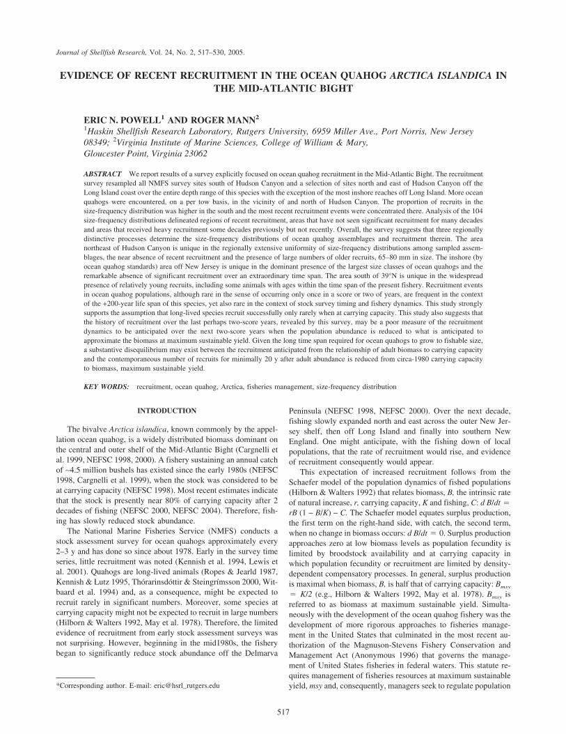
The NMFS conducted a survey of ocean quahogs in the sum-mer of 2002 (NEFSC 2004) The recruitment survey resampled asubset of NMFS survey sites during September 14 to 19 2002This subset included all sites yielding live ocean quahogs in the2002 NMFS survey south of Hudson Canyon and a selection ofsites north and east of Hudson Canyon off the Long Island coastnearly as far east as Montauk New York Sampling covered theentire depth range of this species over this geographic region withthe exception of the most inshore reaches off Long Island The FVChristie homeport Ocean City Maryland was used as the surveyvessel Sampling sites are shown in Figure 1

To catch ocean quahogs lt75 mm a number of modificationswere made to the vessel A typical quahog dredge has a bar spacingtoo large to catch ocean quahogs in the desired size range Clamscaught by the dredge are dropped into a hopper after dredge re-trieval From the hopper the clams move up a belt and then acrossa set of rollers or over a shaker with bar spacings that permitefficient sorting of small material single shells undersized clamsand most bycatch from clams of market size Clams are thenmoved by belt to cages in the hold To conduct the recruitmentsurvey 3 modifications were made to this system (1) The dredgewas lined with chicken wire of 254-cm diameter Clams 25 mmcould not pass through this mesh The chicken wire was affixed tothe bars of the dredge by metal ties and cable ties The metal tiesworked best but the cable ties held up for a surprisingly long timeThe dredge was lined with chicken wire on both sides the bottomand top the door at the back of the dredge and the angled lowerportion of the dredge just behind the knife Thus the entire dredgewas lined The integrity of the chicken wire was examined aftereach tow and occasional repairs were made Repairs were rarelyrequired except for the chicken wire stretched over the front end ofthe dredge just behind the knife It was necessary to catch this wire

daggerThe reader is cautioned that we have relied on age-size relationshipspublished in Murawski et al (1982) and Fritz (1991) as guides to theapproximate ages of ocean quahogs in various size classes We do soprimarily to couch processes in order of occurrence and to evoke someappreciation of time scale We make no claim as to the accuracy of thedating of specific events only that specific events did occur and that thesecan be ordered in time and we point out that Lewis et al (2001) and Sagerand Sammler (1983) have reported more rapid growth rates on GeorgesBank that would compress by about 50 the age ranges referred tothroughout this contribution

Figure 1 Location of sampling stations for the ocean quahog recruit-ment survey

POWELL AND MANN518

between two knife blades to prevent it from pulling away from theknife (2) The shaker was bypassed by means of a metal shootaffixed to the shaker and extending from the hopper belt to the beltrunning along the deck to the hold This metal shoot permitted theentire contents of the dredge to be moved from the hopper to thebelt on the deck (3) The water jets that normally are oriented towash material through the shaker were reoriented to wash materialdown the shoot to the belt on the deck

A trial run was conducted on April 20 2002 Tows of variousdurations from 30 sec to 2 min were conducted Knife depths of51 cm to 102 cm were examined Tow speed was maintainedapproximately at the industry standard of 56 km hrminus1 Test towsrevealed that the dredge could be nearly filled to capacity withmaterial in about 2 min on bottom This quantity of material couldnot be efficiently processed onboard Consequently tows weretimed to be about 1 min on bottom Catches using a knife bladedepth of 51 cm were obviously smaller than for deeper bladedepths A blade depth of 76ndash102 cm is typical for industry ves-sels A 1-min tow with a knife blade depth of 102 cm could beprocessed onboard Thus this towing procedure was adopted forall survey tows

Swept areas can be calculated routinely from the time on bot-tom and the width of the dredge (NEFSC 2000) 254 cm in the caseof the FV Christie For tows of 3 min or more such swept areasare accurate because the degree of uncertainty as to the time on andoff bottom does not exceed 10 sec less than 10 of total tow timeHowever for a 1-min tow the degree of uncertainty is proportion-ately much larger Thus quantification of catch by swept area wasnot attempted For this reason most analyses were conducted afterstandardization of catch to 100 clams towminus1 Numbers per m2 arenot reported However because all tows were conducted in a simi-lar manner we in a few analyses assume that time on bottom wassimilar for all towsDagger

Processing of a dredge haul was conducted as follows Thevessel steamed to the designated point The dredge was deployedand then retrieved after 1 min on the bottom The contents weredumped into the hopper Hopper and deck belt speed were then setso that the material coming out of the hopper could be efficientlysorted by two individuals while it traversed the deck belt andfinally was flushed back overboard Sorting efficiency waschecked by setting belt speed such that the first sorter picked outnearly all of the ocean quahogs leaving the second sorter little tofind If the second sorter began to find more than the occasionalclam the belt speed was lowered permitting the first sorter moretime to sort through the load Sorting time for a typical dredge haulvaried between 30 min and 1 h Teaming time between stationswas also about this long so that processing on deck was nearlycontinuous during the cruise

All ocean quahogs regardless of size were sorted out In mostcases all ocean quahogs were measured to the nearest 1 mm inlongest dimension using a measuring board In a few tows thetotal number of quahogs exceeded 300 even in a 1 min tow Inthese cases the larger quahogs exceeding 70ndash80 mm depending on

the tow were subsampled In all cases all quahogs lt70 mm weremeasured

Data Analysis

Size-frequency distributions were constructed in 1-mm inter-vals For convenience in some figures these data have been col-lapsed into 5-mm size classes

To examine the relationships in size-frequency distribution be-tween sites a principal component analysis (PCA) was run Forconvenience in this case ocean quahogs were lumped into 5-mmcategories Size-frequencies were than standardized to the numberin each 5-mm size class per 100 individuals caught in the towthereby giving each tow equal weight PCA was conducted withorthogonal rotation on data further standardized to a mean of zeroand variance of 1

Statistical analyses focused on ANCOVA using factor scores asthe dependent variables the total number of clams caught per towas the covariate and depth zone and latitudinal zone as maineffects Sampled depths were allocated to 1 of 3 depth zones forthese analyses lt43 m 43ndash55 m and gt55 m This depth zonationallocated a relatively even distribution of stations into each zone29 30 and 45 respectively Stations were allocated to 4 geographiczones based on degree of north latitude gt40deg 39deg to 40deg 38deg to39deg and lt38deg This zonation also allocated stations relativelyevenly 27 32 34 and 11 respectively The lowermost zone wassomewhat underrepresented but was important to be maintainedseparate because it encompasses an area off the Delmarva Penin-sula that received significant fishing pressure early in the oceanquahog fisheryrsquos history during the mid-1980s and as it marks thesouthernmost extension of the geographic range (Dahlgren et al2000) A posteriori least-square means tests were used to identifysignificant components within the ANCOVA

We caution the reader concerning the use of total catch as thecovariate The large time differential between the time of collec-tion and the time of settlement suggests that one should use a totalabundance of prior decades These data are not available As aconsequence the assumption is made that adult abundance haschanged relatively little between the time of collection and thetime of settlement Over the whole stock this assumption is rea-sonable because present-day biomass is about 80 of that presentcirca-1980 (NEFSC 2004) However in some areas such as Del-marva this assumption is much less valid Nevertheless an indi-cation of a relationship between recruitment and adult abundancecan only be obtained in this way

RESULTS

Abundance

The number of ocean quahogs caught in a 1-min tow variedfrom 0ndash1061 (Fig 2) Larger catches occurred farther northCatches were significantly higher north of 40degN latitude than far-ther south (Table 1) Catches were also significantly higher atdepths deeper than 43 m (Table 1) When only the smaller portionof the size-frequency distribution was assessed those clams lt80mm catches varied by geographic region but no longer by depth(Table 1) Many more small quahogs were caught north of 40degNlatitude than in regions farther south (Table 1)

Proportionately more clams lt80 mm were caught south of38degN latitude however (Table 1) Proportionately fewer clamswere caught between 38degN and 39degN than elsewhere Interestingly

DaggerIn passing as all but a few of our sites were NMFS survey sites andbecause our dredge and the NMFS dredge were quantitative for clams gt80mm the number of clams caught below 80 mm might be quantitated usingthe ratio of 80-mm clams in our tows and those in the 2002 NMFSsurvey catch The NMFS survey is quantitated using dredge depletionexperiments to estimate dredge efficiency (NEFSC 1998 2000 2004)

EVIDENCE OF RECRUITMENT IN ARCTICA ISLANDICA 519

the proportion of small clams was higher south of 38degN latitudethan north of 39degN even though the abundance of small clams washighest in the more northern regions (Table 1) The deeper depthzone gt55 m had proportionately more small clams (Table 1)

End-member Size-frequency Distributions

Characteristic or end-member size-frequency distributionswere constructed by cumulating the size-frequency distributionsfor ocean quahog assemblages from stations with PCA factor

scores exceeding 10 To accomplish this PCA analysis was con-ducted using the entire size-frequency distribution for all samplesafter standardization to weight each sample equally The first fourPCA factors determining the four principal end-member size-frequency distributions accounted for 58 of the total variationEach of these PCA factors was determined primarily by the cor-relations between a set of the twenty-four 5-mm size classes thatserved as the database for the PCA Those stations with PCAscores exceeding 10 for a given PCA factor represented stationswith size-frequency distributions dominated by the size classesdetermining that PCA axis By this means the complex of over100 individual size frequencies could be interpreted in terms of afew dominant size-frequency patterns

A series of the smallest size classes between 16 and 35 mm andbetween 41 and 45 mm loaded most heavily on Factor 1 Thesummary size-frequency distribution cumulating all stationsachieving a factor score exceeding 10 for Factor 1 is shown inFigure 3 This size-frequency distribution has 2 modes Stationswith high Factor 1 scores contain a substantial fraction of smallindividuals less than 60 mm in size and a second mode compris-ing individuals 86ndash100 mm in size

The summary size-frequency distribution for assemblages withFactor 2 scores exceeding 10 shows a single mode in the range66ndash95 mm (Fig 3) Ocean quahogs in the size range 66ndash80 mmwere primary determinants of Factor 2 scores and account formost of the single mode in the size-frequency diagram shownin Figure 3 It is interesting that this single mode falls betweenthe two modes present in the end-member size-frequency distri-bution for ocean quahog assemblages scoring highest for Factor 1(Fig 3)

The largest ocean quahog size classes 106ndash130 mm loadedmost heavily on Factor 3 Assemblages scoring gt10 on this factorhad a single primary mode in their summary size-frequency dis-tribution between 96 mm and 130 mm (Fig 4) Thus the first 3

TABLE 1

Results of ANOVA analysis using as the dependent variable the number of clams caught per tow This analysis assumes an equivalent sweptarea for each tow This assumption is further discussed in the Methods section Depth zones and geographic regions are defined in the

Methods section Ratio is the fraction of clams lt80 mm Results of least-square means tests are shown for significant main effects mdash notsignificant at = 005 interaction term

Sizes lt80 mm All Size Classes Ratio

Depth Zone mdash P 0028a P 0018b

Geographic Region P 0001c P lt 00001d P 00032e

DepthRegion mdash mdash mdash

(a) 43ndash55 m lt43 m (c) 39ndash40deg 38ndash39deg lt38deg

gt55 m mdash P 0025 gt40deg P 00013 P 00002 P 0034243ndash55 m P 0016 39ndash40deg mdash mdash

38ndash39deg mdash

(b) 43ndash55 m lt43 m (d) 39ndash40deg 38ndash39deg lt38deg

gt55 m P 0041 P 00057 gt40deg P 0002 P 00001 P 0002543ndash55 m mdash 39ndash40deg mdash mdash

38ndash39deg mdash

(e) 39ndash40deg 38ndash39deg lt38deg

gt40deg mdash P 0005 mdash39ndash40deg P 006 P 003738ndash39deg P 00011

Figure 2 Numbers of ocean quahogs Arctica islandica captured in a1-min tow during the recruitment survey

POWELL AND MANN520

factors described ocean quahog assemblages composed of (1)small and moderately-large individuals (2) medium-sized indi-viduals and (3) large individuals

The final and fourth factor was primarily defined by quahogs inthe size range 36ndash40 mm 51ndash55 mm and 61ndash65 mm The sum-mary size-frequency distribution for assemblages scoring high onFactor 4 is similar to assemblages scoring high on Factor 1 (Fig 4)in that it is bimodal and the upper mode contains individuals in the86ndash100 mm size range however the smaller mode has propor-tionately more larger individuals 36ndash65 mm and the size-frequency distribution has proportionately fewer clams in the up-per mode 86ndash100 mm

Depiction in factor space of the 104 assemblages sampled dem-onstrates that the assemblages fall smoothly on a mixing curvedefined by Factors 1 2 and 3 with Factor 1 assemblages containingproportionately the smallest individuals and Factor 3 assemblagescontaining proportionately the largest individuals (Fig 5) Theextent to which assemblages fall off the Factor 2-Factor 3 axisdescribes the importance of small ocean quahogs in the assem-blagersquos size-frequency distribution The extent to which assem-blages fall off the Factor 1-Factor 2 axis describes the importanceof large ocean quahogs in the assemblagersquos size-frequency distri-bution All assemblages represent some mixture of the three pri-mary end-member size-frequency distributions with the majoritymixing Factor 1 with the moderately-sized animals of Factor 2 orwith the large animals of Factor 3

Geographic Distribution and Statistical Relationships

Assemblages scoring high on one of the four factors were notrandomly distributed in geographic space Factor 1 described a

series of assemblages characterized by a bimodal size-frequencydistribution in which one mode included the smallest size classescollected and the other mode contained relatively large individualsThe distribution of stations yielding ocean quahogs in this size-

Figure 3 Summary size-frequency distributions for all stations withfactor scores gt10 for Factor 1 or Factor 2 Size classes are in 5-mmincrements Thus size class 1 represents clams gt0ndash5 mm size class 2clams gt5ndash10 mm etc

Figure 4 Summary size-frequency distributions for all stations withfactor scores gt10 for Factor 3 or Factor 4 Size classes are in 5-mmincrements Thus size class 1 represents clams gt0ndash5 mm size class 2clams gt5ndash10 mm etc

Figure 5 The location of stations in factor space End-member size-frequency distributions are shown in Figures 3 and 4 Diffusion ofstations off the Factor 2-Factor 3 axis is a function of the importanceof the smallest ocean quahog size classes in the size-frequency distri-bution Diffusion of stations off the Factor 1-Factor 2 axis is a functionof the importance of the largest ocean quahog size classes in the size-frequency distribution

EVIDENCE OF RECRUITMENT IN ARCTICA ISLANDICA 521

frequency distribution was strongly determined by depth and lati-tude (Fig 6 Table 2) Stations deeper than 55 m yielded signifi-cantly more examples of this type of size-frequency distributionthan shallower stations Assemblages scoring high on Factor 1were predominately distributed south of Atlantic City and mostlysouth of Delaware Bay (Fig 6) Stations south of 38degN weresignificantly more likely to be characterized by ocean quahogswith this type of size-frequency distribution (Table 2) Total catchwas a significant covariate This type of size-frequency distribu-tion tended to occur in locations where ocean quahogs were lessabundant Interaction terms between combinations of geographicregion depth zone and total catch were consistently highly sig-nificant (Table 2) Thus considerable variability existed in thedistribution of small quahogs within geographic regions acrossdepths and with respect to total catch

Assemblages scoring high on Factor 2 and thus containingmostly individuals of intermediate size 66ndash95 mm occurred pri-marily northeast of Hudson Canyon (Fig 7) However no maineffect was significant for Factor 2 (Table 2) Perusal of Figure 7suggests that the apparent absence of a significant effect of geo-graphic region on the distribution of assemblages of this type wascaused primarily by the failure of the latitudinal zones as definedin degree intervals to adequately describe the spatial distributionof stations with assemblages characterized by this size-frequencydistribution Least-square means analysis revealed that stationsbetween 38degN and 39degN were significantly less likely to haveassemblages with this type of size-frequency distribution than sta-

TABLE 2

Results of ANCOVA analysis using as the dependent variable the four PCA factors obtained using the complete standardized size-frequencydistribution for each tow Depth zones and geographic regions are defined in the Methods section Total catch was used as a covariate mdash

not significant at = 005 interaction term

Factor 1 Factor 2 Factor 3 Factor 4

Depth Zone P lt 00001a mdash P 0036b P 0029c

Geographic Region P lt 00001d mdashe mdashf P 0023g

DepthRegion P lt 00001 mdash mdash mdashTotal Catch P lt 00001 mdash mdash P 00064Total CatchDepth P lt 00001 mdash mdash P 00078Total CatchRegion P lt 00001 mdash mdash P 0013Total CatchDepthRegion P lt 00001 mdash mdash P 0035

(a) 43ndash55 m lt43 m (d) 39ndash40deg 38ndash39deg lt38deg

gt55 m P lt 00001 P lt 00001 gt40deg mdash mdash P lt 0000143ndash55 m mdash 39ndash40deg mdash P lt 00001

38ndash39deg P lt 00001

(b) 43ndash55 m lt43 m (e) 39ndash40deg 38ndash39deg lt38deg

gt55 m mdash mdash gt40deg mdash P 00063 mdash43ndash55 m P lt 00001 39ndash40deg mdash mdash

38ndash39deg mdash

(c) 43ndash55 m lt43 m (f) 39ndash40deg 38ndash39deg lt38deg

gt55 m P 0003 P 0002 gt40deg P 00004 mdash mdash43ndash55 m mdash 39ndash40deg P 0012 mdash

38ndash39deg mdash

(g) 39ndash40deg 38ndash39deg lt38deg

gt40deg mdash mdash P 0001839ndash40deg mdash P 000238ndash39deg P 0003

Figure 6 The geographic distribution of stations with high Factor 1scores (Fig 3) Factor 1 is weighted most heavily by the smallest oceanquahog size classes Circle diameter is nonlinearly proportional tofactor score Circle diameter is calculated as e(Factor1)10 Legend showsthe size of circles with factor scores of minus23 00 and +23

POWELL AND MANN522

tions north of 40degN (Table 2) Further perusal of Figure 7 shows thatthis zone of low probability actually extends northward to sim395degN

Factor 3 described size-frequency distributions composednearly exclusively of the largest individuals These assemblagespredominated on the inshore half of the cross-shelf distribution ofthis species (Fig 8) These assemblages were significantly morecommon at depths lt43 m (Table 2) Geographic distribution didnot exert a significant effect overall Lease-square means analyseshowever revealed that assemblages with this type of size-frequency distribution occurred more commonly between 39degNand 40degN than north of 40degN or between 38degN and 39degN (Table 2)Thus stations with populations of this type were most common offthe New Jersey coast (Fig 8)

Neither Factors 2 nor 3 were significantly influenced by totalcatch Neither of these factors were characterized by an abundanceof ocean quahogs less than 65 mm in their size-frequency distri-bution Factor 4 assemblages in contrast were characterized by alarge proportion of such small animals As with Factor 1 assem-blages that were also so characterized Factor 4 assemblages weresignificantly influenced by total catch (Table 2) Moreover likeFactor 1 assemblages and also unlike Factors 2 and 3 assemblagesinteraction terms between depth zone geographic region and totalcatch were routinely significant (Table 2) Trends with depth andlatitude were nearly opposite of trends identified with Factor 1assemblages Assemblages with high Factor 4 scores were distrib-uted more uniformly with latitude although more commonly ob-served in the south they also tended to occur in the central to outerportion of the cross-shelf distribution (Fig 9) Stations character-ized by assemblages with Factor 4-type size-frequency distribu-tions were significantly more common at depths shallower than 55m particularly common in the 43ndash55 m depth zone and occurredsignificantly more frequently at latitudes north of 38degN and southof 40degN (Table 2 Fig 9)

End-member Size-frequency Distributions Smaller Size Classes

Those clams lt80 mm in size also were analyzed separately todistinguish different modes and tempos of recruitment The firstfour PCA factors explained 54 of the total variation in the dis-

Figure 9 The geographic distribution of stations with high Factor 4scores (Fig 4) Factor 4 is weighted most heavily by the larger of thesmaller ocean quahog size classes size classes intermediate betweenthose loading on Factors 1 and 2 Circle diameter is nonlinearly pro-portional to factor score Circle diameter is calculated as e(Factor4)10Legend shows the size of circles with factor scores of minus23 00 and +23

Figure 7 The geographic distribution of stations with high Factor 2scores (Fig 3) Factor 2 is weighted most heavily by ocean quahogs ofintermediate size 66ndash95 mm Circle diameter is nonlinearly propor-tional to factor score Circle diameter is calculated as e(Factor2)10Legend shows the size of circles with factor scores of minus23 00 and +23

Figure 8 The geographic distribution of stations with high Factor 3scores (Fig 4) Factor 3 is weighted most heavily by the largest oceanquahog size classes Circle diameter is nonlinearly proportional tofactor score Circle diameter is calculated as e(Factor3)10 Legend showsthe size of circles with factor scores of minus23 00 and +23

EVIDENCE OF RECRUITMENT IN ARCTICA ISLANDICA 523

tribution of these smaller clams among the sampled assemblagesincluding PCA Factors 5 and 6 raised this value to 70

Assemblages scoring high on Factor 1 were characterized by arange of sizes of small clams between 25 and 80 mm (Fig 10)However size classes in the range 16ndash35 mm principally definedwhich assemblages scored highest on Factor 1 Consequentlythese assemblages were characterized by temporally consistent re-cruitment as well as the most recent recruitment events

The remaining factors describe size-frequency distributions inwhich a narrower size range of small clams contributed the bulk ofthe lt80-mm complement of the assemblage For example mostsmall clams in assemblages with high Factor 2 scores were 50ndash60mm in size (Fig 10) End-member size-frequency distributionsdescribed by Factors 5 and 6 like Factor 2 were characterized bystrong size-restricted modes (Fig 11) Those assemblages withhigh Factor 5 scores contained a disproportionately large numberof small ocean quahogs 41ndash45 mm in size (Fig 11) Those assem-blages with high Factor 6 scores contained a disproportionatelylarge number of small ocean quahogs 61ndash65 mm in size (Fig 11)

Populations with high Factor 3 and 4 scores were intermediatebetween the single-mode extreme of Factors 2 5 and 6 and thecontinuous recruitment extreme of Factor 1 Factor 3 size-frequency distributions were relatively enriched in animals 66ndash70mm although most size classes 46ndash80 mm were present (Fig 12)Factor 4 size-frequency distributions were relatively enriched inanimals 46ndash50 mm although again most size classes 46ndash80 mmwere present (Fig 12)

Statistical Relationships Smaller Size Classes

Small ocean quahogs were caught in 93 of 104 stations All ofthe remaining 11 stations with assemblages solely comprisingindividuals 80 mm were distributed along the inner edge of thedepth range for ocean quahogs south of Hudson Canyon (Fig 13)

Factor 1 represents size-frequency distributions characterizedby a wide range and a relatively even apportionment of size classesunder 80 mm Assemblages with this size structure are character-istic of areas recruiting relatively continuously The distribution ofstations with populations having this type of size-frequency dis-tribution was significantly influenced by depth and geographicregion (Table 3) Assemblages with more or less continuous re-cruitment were more frequently encountered at depths gt55 m andnear the southern end of the speciesrsquo range south of 38degN (Fig 13)

Factor 2 represents a series of assemblages in which most smallindividuals lt80 mm were 50ndash60 mm in size Assemblages that hadthis characteristic size structure were significantly more commonat depths lt43 m but just barely so (Table 3) Why the relationshipwith depth is weak is explained by the strong geographic depen-dency demonstrated in the distributional pattern of these assem-blages Size-frequency distributions of this type were encounteredsignificantly more often between 38degN and 40degN (Table 3 Fig14) Shallow assemblages falling outside of this latitudinal bandhad no instances of this type of size-frequency pattern

Factor 3 represents a set of assemblages in which a range ofsmall size classes were present but in which ocean quahogs 66ndash70mm in size were disproportionately represented Neither depth norgeographic region significantly influenced the distribution of as-semblages with this type of size structure (Table 3) Stations of this

Figure 10 Summary size-frequency distributions for all stations withfactor scores above 10 for Factors 1 and 2 based on the analysis onlyof ocean quahogs lt80 mm in size Size classes are in 5-mm incrementsThus size class 1 represents clams gt0ndash5 mm size class 2 clams gt5ndash10mm etc

Figure 11 Summary size-frequency distributions for all stations withfactor scores above 10 for Factors 5 and 6 based on the analysis onlyof ocean quahogs lt80 mm in size Size classes are in 5-mm incrementsThus size class 1 represents clams gt0ndash5 mm size class 2 clams gt5ndash10mm etc

POWELL AND MANN524

sort are scattered throughout much of the Mid-Atlantic Bight (Fig15) Factor 4 assemblages are similar in size structure to Factor 3assemblages except that more of the individuals fall in the 46ndash50mm range Depth did not significantly influence the distributionalpattern The frequency of occurrence was somewhat higher be-tween 38degN and 39degN than above 40degN (Table 3) however theseassemblages were distributed throughout much of the geographicrange south of 40degN (Fig 16)

Factor 5 described a size-frequency structure with a dispropor-tionately large number of small ocean quahogs 41ndash45 mm in sizeThe distribution of stations with ocean quahog assemblages withsize characteristics of this type was not significantly influenced bydepth or geographic region (Table 3) although visually such sta-tions were somewhat rarer north of 40degN (Fig 17) Factor 6 de-scribed a size-frequency structure with a disproportionately largenumber of small ocean quahogs 61ndash65 mm in size Depth was asignificant determinant of the distribution of assemblages so char-acterized (Table 3) however an a posterior test did not localize thereason for the significant main effect Geographic region did notsignificantly influence distribution (Table 3) Visually stationssupporting assemblages of this type were distributed throughoutthe Mid-Atlantic with shallower stations seemingly more likely tobe represented (Fig 18)

DISCUSSION

Perspective

Population size frequencies integrate the recent record of re-cruitment growth and mortality of the comprising cohorts of in-

dividuals (Hallam 1972 Craig amp Oertel 1966) For animals withlong life spans the frequency of recruitment can be a particularlyimportant determining factor Ocean quahogs Arctica islandicaare among the longest-lived invertebrates (Forster 1981 Powell ampCummins 1985 Heller 1990 Callender amp Powell 1997) livingupwards of 200 y (Ropes amp Jearld 1987 Fritz 1991) The speciesis boreal amphi-Atlantic (Dahlgren et al 2000) From this perspec-tive the intrusion of a substantial stock of ocean quahogs south-ward along the Mid-Atlantic coast of the United States is remark-able (Dahlgren et al 2000) One might anticipate that this popu-lation would recruit less predictably and that in fact portions of itmight not be self-sustaining but depend on more northerly spawnSuch is often the character of populations at the edge of a speciesrsquorange Although northeast-coast populations containing small qua-hogs have been reported (Murawski amp Serchuk 1979 Rowell et al1990 Ropes et al 1984 Brey et al 1990) and reproduction andlarval transport in the Mid-Atlantic have been studied (Jones 1981Mann 1982 Mann 1986) the notion that these populations recruitrarely has achieved some renown (Fogarty 1981 Kennish amp Lutz1995 Fritz 1991 NEFSC 1995) Lewis et al (2001) documentedan increase in recruitment on Georges Bank since the 1980s butnoted as well the apparently low number of recruits in the areaof the Mid-Atlantic Bight and the aperiodicity of recruitmentthroughout much of the western Atlantic This contrasts to anapparently more predictable recruitment in Icelandic populations(Thoacuterarinsdoacutettir amp Joacutehannesson 1996)

The apparent rarity of recruitment west and south of GeorgesBank however has profound implications for the ocean quahog

Figure 12 Summary size-frequency distributions for all stations withfactor scores above 10 for Factors 3 and 4 based on the analysis onlyof ocean quahogs lt80 mm in size Size classes are in 5-mm incrementsThus size class 1 represents clams gt0ndash5 mm size class 2 clams gt5ndash10mm etc

Figure 13 The geographic distribution of stations with high Factor 1scores (Fig 10) Factor 1 is weighted most heavily by small oceanquahogs in the size range 16ndash35 mm but size-frequencies scoring highon Factor 1 were characterized by having a range of sizes of smallclams between 25 and 80 mm Circle diameter is nonlinearly propor-tional to factor score Circle diameter is calculated as e(Factor1)10Legend shows the size of circles with factor scores of minus23 00 and +23Crosses indicate stations where no ocean quahogs lt80 mm were col-lected

EVIDENCE OF RECRUITMENT IN ARCTICA ISLANDICA 525

fishery that began in earnest in the early 1980s and now has ayearly quota of 45 million bushels (NEFSC 2000) The presenceof the fishery in turn has profound implications for ocean quahogpopulation dynamics In early stock assessments a so-called min-

ing model was used (NEFSC 1995) This model assumed thatrecruitment was sufficiently rare that population dynamics couldbe approximated by the process of the lowering of abundance byfishing This view in fact has solid theoretical roots in the con-

TABLE 3

Results of ANCOVA analysis using as the dependent variable the six PCA factors obtained using the standardized size-frequencydistributions for each tow with the size classes restricted to animals lt80 mm Depth zones and geographic regions are defined in the

Methods section The covariate total catch was the total of all ocean quahog size classes not just those lt80 mm mdash not significant at = 005 interaction term

Factor 1 Factor 2 Factor 3 Factor 4 Factor 5 Factor 6

Depth Zone P lt 00001a mdashb mdash mdash mdash P 0036Geographic Region P lt 00001c P lt 00001d mdash mdashe mdash mdashDepthRegion P lt 00001 mdash mdash mdash mdash mdashTotal Catch P lt 00001 mdash mdash mdash mdash mdashTotal CatchDepth P lt 00001 mdash mdash mdash mdash mdashTotal CatchRegion P lt 00001 P 00035 mdash mdash mdash mdashTotal CatchDepthRegion P lt 00001 P 0022 mdash mdash mdash mdash

(a) 43ndash55 m lt43 m (c) 39ndash40deg 38ndash39deg lt38deg

gt55 m P lt 00001 P lt 00001 gt40deg mdash mdash P lt 0000143ndash55 m mdash 39ndash40deg mdash P lt 00001

38ndash39deg P lt 00001

(b) 43ndash55 m lt43 m (d) 39ndash40deg 38ndash39deg lt38deg

gt55 m mdash mdash gt40deg P 00001 mdash mdash43ndash55 m P 0048 39ndash40deg P 0025 mdash

38ndash39deg mdash

(e) 39ndash40deg 38ndash39deg lt38deg

gt40deg mdash P 0049 mdash39ndash40deg mdash mdash38ndash39deg mdash

Figure 14 The geographic distribution of stations with high Factor 2scores (Fig 10) Most small clams in populations with high Factor 2scores were 50ndash60 mm in size Circle diameter is nonlinearly propor-tional to factor score Circle diameter is calculated as e(Factor2)10Legend shows the size of circles with factor scores of minus23 00 and +23

Figure 15 The geographic distribution of stations with high Factor 3scores (Fig 12) Factor 3 size-frequencies were relatively enriched inanimals 66ndash70 mm Circle diameter is nonlinearly proportional tofactor score Circle diameter is calculated as e(Factor3)10 Legend showsthe size of circles with factor scores of minus23 00 and +23

POWELL AND MANN526

cepts of carrying capacity and maximum sustainable yield Oneassumes that the ocean quahog population was at or near carryingcapacity prior to the fishery beginning circa 1980 (NEFSC 2000)One characteristic of such populations is that recruitment balances

mortality (Hilborn amp Walters 1992) For a long-lived species witha low mortality rate such as Arctica islandica the necessary cor-ollary is that the rate of recruitment must be extremely low atcarrying capacity Thus a fishery at its inception even if operatingsustainably would appear to be mining A sequitur is that recruit-ment should rise as population biomass declines to the level an-ticipated at maximum sustainable yield

The first problem confronting the search for ocean quahogrecruitment is delimiting the size classes to which the term ldquore-cruitrdquo will apply The fishery for the most part targets oceanquahogs 80 mm in length Animals exceeding 70 mm in lengthmay already exceed 40 y in age (Murawski et al 1982 Fritz 1991)The survey gear used by the NMFS probably catches ocean qua-hogs in the range of 75 mm or larger quantitatively and withequivalent catchability although a precise measure of size biasdoes not exist Thus from the perspective of the fishery and theNMFS survey the term recruit might apply to quahogs lt70ndash80mm in length In this study we choose 80 mm as a convenientdemarcation

Ocean Quahog Size-frequency Composition

The recruitment survey covered the majority of ocean quahoghabitat from the southern end of the speciesrsquo range off Virginia tothe continental shelf off the eastern end of Long Island Samplingcovered the entire depth range of this species over this geographicregion with the exception of the most inshore reaches off LongIsland Lewis et al (2001) independently reported information forocean quahogs on Georges Bank The necessity of conductingextremely short tows the concomitant and inescapable uncertaintyas to the distance traveled over the bottom by the dredge and thelikely nonlinearity in catchability as the dredge fills hamper quan-titative analysis The alternative a reliance on analysis by propor-

Figure 17 The geographic distribution of stations with high Factor 5scores (Fig 11) Those stations with high Factor 5 scores contained adisproportionately large number of small ocean quahogs 41ndash45 mm insize Circle diameter is nonlinearly proportional to factor score Circlediameter is calculated as e(Factor5)10 Legend shows the size of circleswith factor scores of minus23 00 and +23

Figure 16 The geographic distribution of stations with high Factor 4scores (Fig 12) Factor 4 size-frequencies were relatively enriched inanimal 46ndash50 mm Circle diameter is nonlinearly proportional to fac-tor score Circle diameter is calculated as e(Factor4)10 Legend showsthe size of circles with factor scores of minus23 00 and +23

Figure 18 The geographic distribution of stations with high Factor 6scores (Fig 11) Those stations with high Factor 6 scores contained adisproportionately large number of small ocean quahog 61ndash65 mm insize Circle diameter is nonlinearly proportional to factor score Circlediameter is calculated as e(Factor6)10 Legend shows the size of circleswith factor scores of minus23 00 and +23

EVIDENCE OF RECRUITMENT IN ARCTICA ISLANDICA 527

tion prevents definitive judgments as to the sustainability of thestock however the routine presence of recruits frequently in rela-tively high proportions in tows taken throughout much of thesurveyed area bespeaks a more dynamic population structure thanmight previously have been supposed

More ocean quahogs were encountered on a per tow basisnorth of about 395degN latitude (Fig 2) This latitudinal gradation inocean quahog abundance is in part because of the fishery that hasdirected more effort for ocean quahogs off the Delmarva Peninsulaand New Jersey than elsewhere This latitudinal gradation in oceanquahog abundance is also due by inference from the larger numberof ocean quahogs lt80 mm to a higher rate of recruitment north ofabout 395degN The simple inference that lower recruitment is ex-pected at the southern extreme of a speciesrsquo range is perhaps nota complete explanation for the observed latitudinal trends Thedata induce a less simplistic view The proportion of recruits in thesize-frequency distribution is higher in the south Thus abundanceis not low in proportion to the density of local broodstock remem-bering the caveat that present-day abundance may not equate toabundance at time of settlement Moreover the most recent re-cruitment events seem to be concentrated in the south Regionaland depth-dependent interactions are also much more common inthe south (Tables 2 3) Thus recruitment seems to be a moredynamic and patchy process in the south Aggregating these ob-servations elicits caution in deducing too much from the largercatches of ocean quahogs lt80 mm in size north of 395degN

As interesting is the distribution of stations where no recruitswere collected These stations are nearly exclusively on the inshoreedge of the depth distribution of ocean quahogs and south ofHudson Canyon (Fig 16) Although a temptation exists to explainsuch a distributional pattern by recent warming trends in the northAtlantic region (eg Menzel amp Fabian 1999 Cook et al 1998Weinberg et al 2002 Kim amp Powell 2004) the age of animals60ndash80 mm sizes also absent from these stations suggests that thistrend is of much longer standing than the warming trend that begancirca 1990 (Cook et al 1998)

Although size-frequency distributions often vary complexlyamong populations of the same species the 104 assemblagessampled in this study evinced remarkably few structural differ-ences Most sampled size-frequency distributions could be definedin terms of three end-member size frequencies (Figs 3 4 5) Twoof these three contained recruits One of these latter two containedrelatively young recruits (65 mm) and larger animals 90ndash105mm and was therefore bimodal The other contained larger re-cruits (66ndash80 mm) and a smaller subset of the larger animals(80ndash95 mm) and was therefore unimodal The third containedextremely large (gt100 mm) and old animals nearly exclusivelyEach individual size-frequency distribution was an admixture invarying proportion of these large old individuals the older recruits(66ndash80 mm) and the younger recruits (65 mm) All fell on amixing diagram defined by these three end members (Fig 5) Noobvious outlier assemblages existed In fact the fourth size-frequency distribution identified by PCA analysis was simply avariant of the first

End-member size-frequency distributions were not just statis-tical constructs These size-frequency distributions were not ran-domly distributed in geographic space Their distribution in geo-graphic space delineated regions of active recruitment over the lastperhaps score of years areas that have not seen significant recruit-ment over perhaps century time scales and areas that receivedheavy recruitment for a period of time perhaps two score years

ago accepting an approximate 30-y age estimate for a 70-mmocean quahog (Murawski et al 1982) The middle continental shelfoff New Jersey along the inner edge of the depth distribution forocean quahogs was disproportionately characterized by assem-blages containing mostly the largest individuals Many of theselocations have seen little recruitment over the last century (Fig 8)once again using age estimates from Murawski et al (1982) Incontrast north and east of Hudson Canyon is an extensive area inwhich substantial recruitment occurred perhaps some two score ormore years ago (Fig 7) but little since Finally the area south of39degN exemplifies a region where relatively recent recruitmentevents have occurred

Overall the survey suggests three regionally distinctive pro-cesses determining the size-frequency distributions of ocean qua-hog assemblages and recruitment therein The area northeast ofHudson Canyon is clearly unique in the regionally extensive uni-formity of size-frequency distributions among sampled assem-blages the near absence of recruitment over the last score or so ofyears and the presence of large numbers of the largest recruits65ndash80 mm in size The inshore (by ocean quahog standards) areaoff New Jersey is unique in the dominant presence of the largestsize classes of ocean quahogs and the remarkable absence of evi-dence of significant recruitment over an extraordinary time spanThe area south of 39degN is unique in the wide-spread presence ofrelatively young recruits some animals with ages in the time spanof the present fishery

Ocean Quahog Recruitment Dynamics

Move the focus now explicitly to the size classes lt80 mm thatrepresent animals that probably recruited sometime in the last two-score years Analysis revealed six end-member size-frequency dis-tributions One of these is characteristic of the larger recruits north-east of Hudson Canyon (Factor 3 Fig 12) although also foundelsewhere (Fig 15) The other five are restricted to the regionsouth of Hudson Canyon Of these five only one comprised abroad relatively evenly apportioned series of size classes (Factor 1Fig 10 13) The remaining four contain single dominant sizeclasses representative of dominant year classes 40ndash45 mm 45ndash5050ndash60 mm and 60ndash65 mm

The distribution of these assemblage types is determined onlyin the broadest sense by latitudinal range or depth zone within theconfines of this survey (Table 3) Only the first is significantlyinfluenced by total quahog abundance Interestingly this one isalso the size-frequency distribution comprising multiple sizeclasses rather evenly apportioned Assemblages with this size-frequency structure tend to be located in the south and offshore atleast somewhat coincident with the region believed to have beenimpacted most by the ocean quahog fishery during the 1980s Thecoincidence of heaviest fishery impact as defined by largest his-torical change in CPUE (NEFSC 1998) and most consistent re-cruitment pattern is perhaps noteworthy

The remaining size-frequency styles tend to be quasi-randomlydistributed within the general region defined by the speciesrsquo south-ern range limit and Hudson Canyon excluding of course much ofthe area inshore off New Jersey where recruitment is rare Thebroad geographic overlap of these size-frequency styles suggeststhat local conditions determine recruitment success within an areawhere recruitment has potential much more frequently than it hassuccess Statistical evaluation reveals that assemblages recruitingoften are associated most frequently with significant interaction

POWELL AND MANN528

terms with depth zone and geographic region and also most ofteninfluenced by local ocean quahog abundance This reinforces theconclusion that recruitment is complex over small spatial scales

CONCLUSION

This survey combined with recent work by Lewis et al (2001)demonstrates clearly that ocean quahog recruitment occursthroughout much of the United States east coast range of the spe-cies These recruitment events however with one exception seemto be rare and aperiodic Recruitment has been more or less con-tinuous of recent only in the southern portion of the ocean qua-hogrsquos range However these recruitment events are not rare incomparison with the animalrsquos life span only in comparison withthe surveys of man When recruitment events occur they can benumerically profound These events also with three exceptionsseem to be a product of local rather than regional or depth-dependent processes That is any local area has potential for re-cruitment every year but the degree to which that potential isrealized is determined by local processes and these local processesnormally militate against the event

Three exceptions are noteworthy First is the inshore edge ofthe speciesrsquo depth range south of Hudson Canyon that includes adisproportionate number of stations with no evidence of recruit-ment Second is the region northeast of Hudson Canyon thatclearly expanded rapidly in population abundance some two-scoreor more years ago but has accreted little since The recruitmentdynamics in this region are unique to the surveyed area of theMid-Atlantic Bight Third is the more consistent recruitment pat-tern observed most often in southern assemblages coincident withthe region most heavily impacted by fishing during the first twodecades of the ocean quahog fishery This coincidence is causalunder the Schaefer theory of population dynamics (Hilborn ampWalters 1992) if these recruits are young enough

We have not attempted to answer the question of sustainabilityof the ocean quahog stock at present fishing levels Fisheries thattarget long-lived animals are frequently difficult to manage sus-tainably What is clear is that the time scale of such an evaluationfor ocean quahogs will strain the capabilities of present fisheriesmodels An unquestionable conclusion from this study is that re-cruitment events although rare in the sense of occurring only oncein a score or two of years are frequent in the context of the+200-year life span of this species yet also rare in the context ofstock survey timing and fishery dynamics Moreover this studystrongly suggests that the application of the Schaefer theory ofpopulation dynamics of fished populations (Hilborn amp Walters1992) to the management of the ocean quahog fishery with itsdefined relationships between carrying capacity and maximumsustainable yield (Bmsy K2) and its assumption that long-lived

species must recruit successfully only rarely when at carrying ca-pacity (Hilborn amp Walters 1992) is meritorious But this studyalso suggests that the history of recruitment over the last perhapstwo-score years revealed by this survey may be a poor measure ofthe recruitment dynamics to be anticipated over the next two-scoreyears when the population abundance is reduced to what is antic-ipated to approximate the biomass at maximum sustainable yieldand recruitment rate is expected consequently to continue to rise

We know only in a general way how old these quahog recruitsare Lewis et al (2001) have shown recently that ocean quahoggrowth rates may vary considerably over their United States rangeAs a consequence we cannot estimate what fraction of the recruitssettled subsequent to the initiation of the fishery circa-1980 usingpublished age-length relationships (eg Murawski et al 1982)The coincidence of the highest numbers of new recruits in the areamost heavily fished at the beginning of the fishery is enticingbecause it meets a basic expectation of fisheries population dy-namics but it cannot yet be judged unquestionably causal What ismore clear is that the recruits observed in this study represent theanimals that must balance fishing mortality when the fishery re-duces ocean quahog biomass to Bmsy an event expected to occur insim20 y In shorter-lived species this balance is obtained by theequilibrium of recruitment at Bmsy with fishing at Bmsy In oceanquahogs over a much longer period of time that same equilibriumalso can be anticipated However a period of time will exist whenthe stock is at Bmsy but recruitment into the fishery is not charac-teristic of that expected at Bmsy That period of time represents amost unusual challenge for fisheries management Obtaining moreinformation on the abundance of ocean quahogs lt80-mm in sizeover the coming decade will be critical in establishing the neces-sary management structure to carry the fishery though this periodof disequilibrium

ACKNOWLEDGMENTS

The authors appreciate the efficiency and competency of theCaptain and crew of the FV Christie who carried out this arduoussampling task in 6 days at sea The authors also wish to thankOliver Donovan Bruce Muller and Peter Smith who helped withsample collection Bruce Muller who helped in data analysis andCaptain Robert Jarnol of the FV Christie who designed the gearand deck modifications to permit lining the dredge with smallmesh wire and the bypassing of the shaker The authors appreciatethe continuing support of the clam stock assessment team atNMFS-Northeast Fisheries Science Center including Jim Wein-berg and Larry Jacobson who provided detailed stations locationsand additional logistical help in cruise planning This research wasfunded by the New Jersey Fisheries Information and DevelopmentCenter The authors appreciate this support

LITERATURE CITED

Anonymous 1996 Magnuson-Stevens Fishery Conservation and Manage-ment Act US Dept Commerce NOAA NMFS NOAA Tech MemNMFS-F SPO-23 121 pp

Brey T W E Arntz D Pauly amp H Rumohr 1990 Arctica (Cyprina)islandica in Kiel Bay (Western Baltic) growth production and eco-logical significance J Exp Mar Biol Ecol 136217ndash235

Callender W R amp E N Powell 1997 Autochthonous death assemblagesfrom chemoautotrophic communities at petroleum seeps paleoproduc-tion energy flow and implications for the fossil record Hist Biol12165ndash198

Cargnelli L M S J Griesbach D B Packer amp E Weissberger 1999Ocean quahog Arctica islandica life history and habitat characteris-tics NOAA Tech Mem NMFS NE-148 12 pp

Cook T M Folli J Klinck S Ford amp J Miller 1998 The relationshipbetween increasing sea-surface temperature and the northward spreadof Perkinsus marinus (Dermo) disease epizootics in oysters EstuarineCoast Shelf Sci 46587ndash597

Craig G amp G Oertel 1966 Deterministic models of living and fossilpopulations of animals Geol Soc Lond 122315ndash355

Dahlgren T G J R Weinberg amp K M Halanych 2000 Phylogeography

EVIDENCE OF RECRUITMENT IN ARCTICA ISLANDICA 529

of the ocean quahog (Arctica islandica) Influences of paleoclimate ongenetic diversity and species range Mar Biol (Berl) 137487ndash495

Fogarty M J 1981 Distribution and relative abundance of the oceanquahog Arctica islandica in Rhode Island Sound and off MartharsquosVineyard Massachusetts J Shellfish Res 133ndash39

Forster G R 1981 A note on the growth of Arctica islandica J MarBiol Assoc UK 61817

Fritz L W 1991 Seasonal condition change morphometrics growth andsex ratio of the ocean quahog Arctica islandica (Linnaeus 1767) offNew Jersey USA J Shellfish Res 1079ndash88

Hallam A 1972 Models involving population dynamics In T J MSchopf editor Models in paleobiology San Francisco CA FreemanCooper and Company pp 62ndash80

Heller J 1990 Longevity in Mollusca Malacologia 31259ndash295Hilborn R amp C J Walters 1992 Fisheries stock assessment choice

dynamics amp uncertainty New York Chapman amp Hall 570 ppJones D S 1981 Reproductive cycles of the Atlantic surf clam Spisula

solidissima and the ocean quahog Arctica islandica off New Jersey JShellfish Res 123ndash32

Kennish M J amp R A Lutz 1995 Assessment of the ocean quahogArctica islandica (Linnaeus 1767) in the New Jersey fishery J Shell-fish Res 1445ndash52

Kennish M J R A Lutz J A Dobarro amp L W Fritz 1994 In situgrowth rates of the ocean quahog Arctica islandica (Linnaeus 1767)in the Middle Atlantic Bight J Shellfish Res 13473ndash478

Kim Y amp E N Powell 2004 Surf clam histopathology survey along theDelmarva mortality line J Shellfish Res 23429ndash441

Lewis C V W J R Weinberg amp C S Davis 2001 Population structureand recruitment of the bivalve Arctica islandica (Linnaeus 1767) onGeorges Bank from 1980ndash1999 J Shellfish Res 201135ndash1144

Mann R 1982 The seasonal cycle of gonadal development in Arcticaislandica from the southern New England shelf Fish Bull 80315ndash326

Mann R 1986 Arctica islandica (Linneacute) larvae active depth regulators orpassive particles Am Malacol Bull Spec Ed 351ndash57

May R M J R Beddington amp J G Shepherd 1978 Exploiting naturalpopulations in an uncertain world Math Biosci 42219ndash252

Menzel A amp P Fabian 1999 Growing season extended in Europe Nature397659

Murawski S A J W Ropes amp F M Serchuk 1982 Growth of the oceanquahog Arctica islandica in the Middle Atlantic Bight Fish Bull8021ndash34

Murawski S A amp F M Serchuk 1979 Shell lengthmdashmeat weight rela-tionships of ocean quahogs Arctica islandica from the Middle Atlanticshelf Proc Natl Shellfish Assoc 6940ndash46

NEFSC 1995 19th northeast regional stock assessment workshop(19th SAW) stock assessment review committee (SARC) consensus

summary of assessments Northeast Fish Sci Cent Ref Doc 95-08221 pp

NEFSC 1998 27th northeast regional stock assessment workshop(27th SAW) stock assessment review committee (SARC) consensussummary of assessments Northeast Fish Sci Cent Ref Doc 98-15

NEFSC 2000 31st northeast regional stock assessment workshop(31st SAW) stock assessment review committee (SARC) consensussummary of assessments Northeast Fish Sci Cent Ref Doc 00-15400 pp

NEFSC 2004 38th northeast regional stock assessment workshop(38th SAW) stock assessment review committee (SARC) consensussummary of assessments Northeast Fish Sci Cent Ref Doc 00-15246 pp

Powell E N amp H C Cummins 1985 Are molluscan maximum life spansdetermined by long-term cycles in benthic communities Oecologia67177ndash182

Ragnarsson S A amp G G Thoacuterarinsdoacutettir 2002 Abundance of oceanquahog Arctica islandica assessed by underwater photography and ahydraulic dredge J Shellfish Res 21673ndash676

Ropes J W amp A Jearld Jr 1987 Age determination of ocean bivalvesIn R C Summerfelt amp G E Hall editors The age and growth of fishAmes Iowa Iowa State Univ Press pp 517ndash530

Ropes J W S A Murawski amp F M Serchuk 1984 Size age sexualmaturity and sex ratio in ocean quahogs Arctica islandica Linneacute offLong Island New York Fish Bull 82253ndash266

Rowell T W D R Chaisson amp J T McLane 1990 Size and age ofsexual maturity and annual gametogenic cycle in the ocean quahogArctica islandica (Linnaeus 1767) from coastal waters in Nova ScotiaCanada J Shellfish Res 9195ndash203

Sager G amp R Sammler 1983 Mathematical investigations into the lon-gevity of the ocean quahog Arctica islandica (Mollusca Bivalvia) IntRev Ges Hydrobiol 68113ndash120

Smolowitz R J amp V E Nulk 1982 The design of an electrohydraulicdredge for clam survey Mar Fish Rev 44(4)1ndash18

Thoacuterarinsdoacutettir G G amp G Joacutehannesson 1996 Shell length-meat weightrelationships of ocean quahog Arctica islandica (Linnaeus 1767)from Icelandic waters J Shellfish Res 15729ndash733

Thoacuterarinsdoacutettir G G amp S A Steingriacutemsson 2000 Size and age at sexualmaturity and sex ratio in ocean quahog Arctica islandica (Linnaeus1767) off northwest Iceland J Shellfish Res 19943ndash947

Weinberg J R T G Dahlgren amp K M Halanych 2002 Influence ofrising sea temperature on commercial bivalve species of the US At-lantic coast Am Fish Soc Symp 32131ndash140

Witbaard R M I Jenness K van der Borg amp G Ganssen 1994 Veri-fication of annual growth increments in Arctica islandica L from theNorth Sea by means of oxygen and carbon isotopes Neth J Sea Res3391ndash101

POWELL AND MANN530

biomass at Bmsy Ocean quahogs are believed to have been at ornear carrying capacity circa 1980 Since then the fishery reducedbiomass to about 80 of carrying capacity (NEFSC 2004) As theocean quahog population continues to be fished down to Bmsy theexpectation of increased recruitment rises and consequently ac-curate estimates of the rate of recruitment become more importantin managing the ocean quahog fishery

The NMFS survey dredge like most commercial dredges doesnot quantitatively catch the smaller size classes Thus the sam-pling gear may not adequately detect recruitment events until therecruits are quite old Despite this limitation recently evidence ofquahog recruitment on Georges Bank has been reported fromNMFS survey samples (Lewis et al 2001) Curiously and perhapsperversely this is also a region of the northeastern Atlantic that hasnot been routinely fished Inasmuch as these observations providea trend counter to the carrying capacity model and recruitment inthe more heavily fished southern populations seemingly remainslow evidence of quahog recruitment continues to be elusive andintuitively abstruse

The limited information on quahog recruitment is primarily afunction of the minimum size caught quantitatively by the surveydredge Although dredge efficiency is inherently less than 100(NEFSC 1998 NEFSC 2000 see also Ragnarsson amp Thoacuterarins-doacutettir 2002) the NMFS survey dredge (Smolowitz amp Nulk 1982)captures ocean quahogs from maximum size sim130 mm down to asize in the range of 70ndash75 mm with about equivalent catchability(NEFSC 1998 Lewis et al 2001) A somewhat larger size rangecut-off is typical for commercial dredges Animals 75-mm long arealready in the range of 40 or more years old (Murawski et al 1982Fritz 1991)dagger This is about twice the age of the fishery so standardsurveys cannot yet provide unequivocal evidence of recruitmentthat has occurred since fishing began and the population waspulled slowly down from carrying capacity

The purpose of this study is to implement a survey explicitlyfocused on ocean quahog recruitment in the Mid-Atlantic BightThe survey targeted animals as small as 25 mm Animals in the25ndash75 mm size range can be expected to have ages in the range ofabout +6ndash40 years and thus some of these clams may have re-cruited since the inception of the fishery circa 1980 As impor-tantly many of them will recruit to the fishery over the next scoreor so years and this recruitment must balance the anticipated fish-ing mortality at Bmsy Bmsy should be reached in another approxi-mately 20 y Put another way when Bmsy is reached the recruitsnecessary to prevent population biomass from dropping belowBmsy will be those in evidence today whereas the greater numberof recruits anticipated to be produced by a population at Bmsy willrequire a further score or more years to impact the fishery Thisdisequilibrium is one of the most serious problems that will facemanagers in the coming decades

METHODS

Survey Approach

The NMFS conducted a survey of ocean quahogs in the sum-mer of 2002 (NEFSC 2004) The recruitment survey resampled asubset of NMFS survey sites during September 14 to 19 2002This subset included all sites yielding live ocean quahogs in the2002 NMFS survey south of Hudson Canyon and a selection ofsites north and east of Hudson Canyon off the Long Island coastnearly as far east as Montauk New York Sampling covered theentire depth range of this species over this geographic region withthe exception of the most inshore reaches off Long Island The FVChristie homeport Ocean City Maryland was used as the surveyvessel Sampling sites are shown in Figure 1

To catch ocean quahogs lt75 mm a number of modificationswere made to the vessel A typical quahog dredge has a bar spacingtoo large to catch ocean quahogs in the desired size range Clamscaught by the dredge are dropped into a hopper after dredge re-trieval From the hopper the clams move up a belt and then acrossa set of rollers or over a shaker with bar spacings that permitefficient sorting of small material single shells undersized clamsand most bycatch from clams of market size Clams are thenmoved by belt to cages in the hold To conduct the recruitmentsurvey 3 modifications were made to this system (1) The dredgewas lined with chicken wire of 254-cm diameter Clams 25 mmcould not pass through this mesh The chicken wire was affixed tothe bars of the dredge by metal ties and cable ties The metal tiesworked best but the cable ties held up for a surprisingly long timeThe dredge was lined with chicken wire on both sides the bottomand top the door at the back of the dredge and the angled lowerportion of the dredge just behind the knife Thus the entire dredgewas lined The integrity of the chicken wire was examined aftereach tow and occasional repairs were made Repairs were rarelyrequired except for the chicken wire stretched over the front end ofthe dredge just behind the knife It was necessary to catch this wire

daggerThe reader is cautioned that we have relied on age-size relationshipspublished in Murawski et al (1982) and Fritz (1991) as guides to theapproximate ages of ocean quahogs in various size classes We do soprimarily to couch processes in order of occurrence and to evoke someappreciation of time scale We make no claim as to the accuracy of thedating of specific events only that specific events did occur and that thesecan be ordered in time and we point out that Lewis et al (2001) and Sagerand Sammler (1983) have reported more rapid growth rates on GeorgesBank that would compress by about 50 the age ranges referred tothroughout this contribution

Figure 1 Location of sampling stations for the ocean quahog recruit-ment survey

POWELL AND MANN518

between two knife blades to prevent it from pulling away from theknife (2) The shaker was bypassed by means of a metal shootaffixed to the shaker and extending from the hopper belt to the beltrunning along the deck to the hold This metal shoot permitted theentire contents of the dredge to be moved from the hopper to thebelt on the deck (3) The water jets that normally are oriented towash material through the shaker were reoriented to wash materialdown the shoot to the belt on the deck

A trial run was conducted on April 20 2002 Tows of variousdurations from 30 sec to 2 min were conducted Knife depths of51 cm to 102 cm were examined Tow speed was maintainedapproximately at the industry standard of 56 km hrminus1 Test towsrevealed that the dredge could be nearly filled to capacity withmaterial in about 2 min on bottom This quantity of material couldnot be efficiently processed onboard Consequently tows weretimed to be about 1 min on bottom Catches using a knife bladedepth of 51 cm were obviously smaller than for deeper bladedepths A blade depth of 76ndash102 cm is typical for industry ves-sels A 1-min tow with a knife blade depth of 102 cm could beprocessed onboard Thus this towing procedure was adopted forall survey tows

Swept areas can be calculated routinely from the time on bot-tom and the width of the dredge (NEFSC 2000) 254 cm in the caseof the FV Christie For tows of 3 min or more such swept areasare accurate because the degree of uncertainty as to the time on andoff bottom does not exceed 10 sec less than 10 of total tow timeHowever for a 1-min tow the degree of uncertainty is proportion-ately much larger Thus quantification of catch by swept area wasnot attempted For this reason most analyses were conducted afterstandardization of catch to 100 clams towminus1 Numbers per m2 arenot reported However because all tows were conducted in a simi-lar manner we in a few analyses assume that time on bottom wassimilar for all towsDagger

Processing of a dredge haul was conducted as follows Thevessel steamed to the designated point The dredge was deployedand then retrieved after 1 min on the bottom The contents weredumped into the hopper Hopper and deck belt speed were then setso that the material coming out of the hopper could be efficientlysorted by two individuals while it traversed the deck belt andfinally was flushed back overboard Sorting efficiency waschecked by setting belt speed such that the first sorter picked outnearly all of the ocean quahogs leaving the second sorter little tofind If the second sorter began to find more than the occasionalclam the belt speed was lowered permitting the first sorter moretime to sort through the load Sorting time for a typical dredge haulvaried between 30 min and 1 h Teaming time between stationswas also about this long so that processing on deck was nearlycontinuous during the cruise

All ocean quahogs regardless of size were sorted out In mostcases all ocean quahogs were measured to the nearest 1 mm inlongest dimension using a measuring board In a few tows thetotal number of quahogs exceeded 300 even in a 1 min tow Inthese cases the larger quahogs exceeding 70ndash80 mm depending on

the tow were subsampled In all cases all quahogs lt70 mm weremeasured

Data Analysis

Size-frequency distributions were constructed in 1-mm inter-vals For convenience in some figures these data have been col-lapsed into 5-mm size classes

To examine the relationships in size-frequency distribution be-tween sites a principal component analysis (PCA) was run Forconvenience in this case ocean quahogs were lumped into 5-mmcategories Size-frequencies were than standardized to the numberin each 5-mm size class per 100 individuals caught in the towthereby giving each tow equal weight PCA was conducted withorthogonal rotation on data further standardized to a mean of zeroand variance of 1

Statistical analyses focused on ANCOVA using factor scores asthe dependent variables the total number of clams caught per towas the covariate and depth zone and latitudinal zone as maineffects Sampled depths were allocated to 1 of 3 depth zones forthese analyses lt43 m 43ndash55 m and gt55 m This depth zonationallocated a relatively even distribution of stations into each zone29 30 and 45 respectively Stations were allocated to 4 geographiczones based on degree of north latitude gt40deg 39deg to 40deg 38deg to39deg and lt38deg This zonation also allocated stations relativelyevenly 27 32 34 and 11 respectively The lowermost zone wassomewhat underrepresented but was important to be maintainedseparate because it encompasses an area off the Delmarva Penin-sula that received significant fishing pressure early in the oceanquahog fisheryrsquos history during the mid-1980s and as it marks thesouthernmost extension of the geographic range (Dahlgren et al2000) A posteriori least-square means tests were used to identifysignificant components within the ANCOVA

We caution the reader concerning the use of total catch as thecovariate The large time differential between the time of collec-tion and the time of settlement suggests that one should use a totalabundance of prior decades These data are not available As aconsequence the assumption is made that adult abundance haschanged relatively little between the time of collection and thetime of settlement Over the whole stock this assumption is rea-sonable because present-day biomass is about 80 of that presentcirca-1980 (NEFSC 2004) However in some areas such as Del-marva this assumption is much less valid Nevertheless an indi-cation of a relationship between recruitment and adult abundancecan only be obtained in this way

RESULTS

Abundance

The number of ocean quahogs caught in a 1-min tow variedfrom 0ndash1061 (Fig 2) Larger catches occurred farther northCatches were significantly higher north of 40degN latitude than far-ther south (Table 1) Catches were also significantly higher atdepths deeper than 43 m (Table 1) When only the smaller portionof the size-frequency distribution was assessed those clams lt80mm catches varied by geographic region but no longer by depth(Table 1) Many more small quahogs were caught north of 40degNlatitude than in regions farther south (Table 1)

Proportionately more clams lt80 mm were caught south of38degN latitude however (Table 1) Proportionately fewer clamswere caught between 38degN and 39degN than elsewhere Interestingly

DaggerIn passing as all but a few of our sites were NMFS survey sites andbecause our dredge and the NMFS dredge were quantitative for clams gt80mm the number of clams caught below 80 mm might be quantitated usingthe ratio of 80-mm clams in our tows and those in the 2002 NMFSsurvey catch The NMFS survey is quantitated using dredge depletionexperiments to estimate dredge efficiency (NEFSC 1998 2000 2004)

EVIDENCE OF RECRUITMENT IN ARCTICA ISLANDICA 519

the proportion of small clams was higher south of 38degN latitudethan north of 39degN even though the abundance of small clams washighest in the more northern regions (Table 1) The deeper depthzone gt55 m had proportionately more small clams (Table 1)

End-member Size-frequency Distributions

Characteristic or end-member size-frequency distributionswere constructed by cumulating the size-frequency distributionsfor ocean quahog assemblages from stations with PCA factor

scores exceeding 10 To accomplish this PCA analysis was con-ducted using the entire size-frequency distribution for all samplesafter standardization to weight each sample equally The first fourPCA factors determining the four principal end-member size-frequency distributions accounted for 58 of the total variationEach of these PCA factors was determined primarily by the cor-relations between a set of the twenty-four 5-mm size classes thatserved as the database for the PCA Those stations with PCAscores exceeding 10 for a given PCA factor represented stationswith size-frequency distributions dominated by the size classesdetermining that PCA axis By this means the complex of over100 individual size frequencies could be interpreted in terms of afew dominant size-frequency patterns

A series of the smallest size classes between 16 and 35 mm andbetween 41 and 45 mm loaded most heavily on Factor 1 Thesummary size-frequency distribution cumulating all stationsachieving a factor score exceeding 10 for Factor 1 is shown inFigure 3 This size-frequency distribution has 2 modes Stationswith high Factor 1 scores contain a substantial fraction of smallindividuals less than 60 mm in size and a second mode compris-ing individuals 86ndash100 mm in size

The summary size-frequency distribution for assemblages withFactor 2 scores exceeding 10 shows a single mode in the range66ndash95 mm (Fig 3) Ocean quahogs in the size range 66ndash80 mmwere primary determinants of Factor 2 scores and account formost of the single mode in the size-frequency diagram shownin Figure 3 It is interesting that this single mode falls betweenthe two modes present in the end-member size-frequency distri-bution for ocean quahog assemblages scoring highest for Factor 1(Fig 3)

The largest ocean quahog size classes 106ndash130 mm loadedmost heavily on Factor 3 Assemblages scoring gt10 on this factorhad a single primary mode in their summary size-frequency dis-tribution between 96 mm and 130 mm (Fig 4) Thus the first 3

TABLE 1

Results of ANOVA analysis using as the dependent variable the number of clams caught per tow This analysis assumes an equivalent sweptarea for each tow This assumption is further discussed in the Methods section Depth zones and geographic regions are defined in the

Methods section Ratio is the fraction of clams lt80 mm Results of least-square means tests are shown for significant main effects mdash notsignificant at = 005 interaction term

Sizes lt80 mm All Size Classes Ratio

Depth Zone mdash P 0028a P 0018b

Geographic Region P 0001c P lt 00001d P 00032e

DepthRegion mdash mdash mdash

(a) 43ndash55 m lt43 m (c) 39ndash40deg 38ndash39deg lt38deg

gt55 m mdash P 0025 gt40deg P 00013 P 00002 P 0034243ndash55 m P 0016 39ndash40deg mdash mdash

38ndash39deg mdash

(b) 43ndash55 m lt43 m (d) 39ndash40deg 38ndash39deg lt38deg

gt55 m P 0041 P 00057 gt40deg P 0002 P 00001 P 0002543ndash55 m mdash 39ndash40deg mdash mdash

38ndash39deg mdash

(e) 39ndash40deg 38ndash39deg lt38deg

gt40deg mdash P 0005 mdash39ndash40deg P 006 P 003738ndash39deg P 00011

Figure 2 Numbers of ocean quahogs Arctica islandica captured in a1-min tow during the recruitment survey

POWELL AND MANN520

factors described ocean quahog assemblages composed of (1)small and moderately-large individuals (2) medium-sized indi-viduals and (3) large individuals

The final and fourth factor was primarily defined by quahogs inthe size range 36ndash40 mm 51ndash55 mm and 61ndash65 mm The sum-mary size-frequency distribution for assemblages scoring high onFactor 4 is similar to assemblages scoring high on Factor 1 (Fig 4)in that it is bimodal and the upper mode contains individuals in the86ndash100 mm size range however the smaller mode has propor-tionately more larger individuals 36ndash65 mm and the size-frequency distribution has proportionately fewer clams in the up-per mode 86ndash100 mm

Depiction in factor space of the 104 assemblages sampled dem-onstrates that the assemblages fall smoothly on a mixing curvedefined by Factors 1 2 and 3 with Factor 1 assemblages containingproportionately the smallest individuals and Factor 3 assemblagescontaining proportionately the largest individuals (Fig 5) Theextent to which assemblages fall off the Factor 2-Factor 3 axisdescribes the importance of small ocean quahogs in the assem-blagersquos size-frequency distribution The extent to which assem-blages fall off the Factor 1-Factor 2 axis describes the importanceof large ocean quahogs in the assemblagersquos size-frequency distri-bution All assemblages represent some mixture of the three pri-mary end-member size-frequency distributions with the majoritymixing Factor 1 with the moderately-sized animals of Factor 2 orwith the large animals of Factor 3

Geographic Distribution and Statistical Relationships

Assemblages scoring high on one of the four factors were notrandomly distributed in geographic space Factor 1 described a

series of assemblages characterized by a bimodal size-frequencydistribution in which one mode included the smallest size classescollected and the other mode contained relatively large individualsThe distribution of stations yielding ocean quahogs in this size-

Figure 3 Summary size-frequency distributions for all stations withfactor scores gt10 for Factor 1 or Factor 2 Size classes are in 5-mmincrements Thus size class 1 represents clams gt0ndash5 mm size class 2clams gt5ndash10 mm etc

Figure 4 Summary size-frequency distributions for all stations withfactor scores gt10 for Factor 3 or Factor 4 Size classes are in 5-mmincrements Thus size class 1 represents clams gt0ndash5 mm size class 2clams gt5ndash10 mm etc

Figure 5 The location of stations in factor space End-member size-frequency distributions are shown in Figures 3 and 4 Diffusion ofstations off the Factor 2-Factor 3 axis is a function of the importanceof the smallest ocean quahog size classes in the size-frequency distri-bution Diffusion of stations off the Factor 1-Factor 2 axis is a functionof the importance of the largest ocean quahog size classes in the size-frequency distribution

EVIDENCE OF RECRUITMENT IN ARCTICA ISLANDICA 521

frequency distribution was strongly determined by depth and lati-tude (Fig 6 Table 2) Stations deeper than 55 m yielded signifi-cantly more examples of this type of size-frequency distributionthan shallower stations Assemblages scoring high on Factor 1were predominately distributed south of Atlantic City and mostlysouth of Delaware Bay (Fig 6) Stations south of 38degN weresignificantly more likely to be characterized by ocean quahogswith this type of size-frequency distribution (Table 2) Total catchwas a significant covariate This type of size-frequency distribu-tion tended to occur in locations where ocean quahogs were lessabundant Interaction terms between combinations of geographicregion depth zone and total catch were consistently highly sig-nificant (Table 2) Thus considerable variability existed in thedistribution of small quahogs within geographic regions acrossdepths and with respect to total catch

Assemblages scoring high on Factor 2 and thus containingmostly individuals of intermediate size 66ndash95 mm occurred pri-marily northeast of Hudson Canyon (Fig 7) However no maineffect was significant for Factor 2 (Table 2) Perusal of Figure 7suggests that the apparent absence of a significant effect of geo-graphic region on the distribution of assemblages of this type wascaused primarily by the failure of the latitudinal zones as definedin degree intervals to adequately describe the spatial distributionof stations with assemblages characterized by this size-frequencydistribution Least-square means analysis revealed that stationsbetween 38degN and 39degN were significantly less likely to haveassemblages with this type of size-frequency distribution than sta-

TABLE 2

Results of ANCOVA analysis using as the dependent variable the four PCA factors obtained using the complete standardized size-frequencydistribution for each tow Depth zones and geographic regions are defined in the Methods section Total catch was used as a covariate mdash

not significant at = 005 interaction term

Factor 1 Factor 2 Factor 3 Factor 4

Depth Zone P lt 00001a mdash P 0036b P 0029c

Geographic Region P lt 00001d mdashe mdashf P 0023g

DepthRegion P lt 00001 mdash mdash mdashTotal Catch P lt 00001 mdash mdash P 00064Total CatchDepth P lt 00001 mdash mdash P 00078Total CatchRegion P lt 00001 mdash mdash P 0013Total CatchDepthRegion P lt 00001 mdash mdash P 0035

(a) 43ndash55 m lt43 m (d) 39ndash40deg 38ndash39deg lt38deg

gt55 m P lt 00001 P lt 00001 gt40deg mdash mdash P lt 0000143ndash55 m mdash 39ndash40deg mdash P lt 00001

38ndash39deg P lt 00001

(b) 43ndash55 m lt43 m (e) 39ndash40deg 38ndash39deg lt38deg

gt55 m mdash mdash gt40deg mdash P 00063 mdash43ndash55 m P lt 00001 39ndash40deg mdash mdash

38ndash39deg mdash

(c) 43ndash55 m lt43 m (f) 39ndash40deg 38ndash39deg lt38deg

gt55 m P 0003 P 0002 gt40deg P 00004 mdash mdash43ndash55 m mdash 39ndash40deg P 0012 mdash

38ndash39deg mdash

(g) 39ndash40deg 38ndash39deg lt38deg

gt40deg mdash mdash P 0001839ndash40deg mdash P 000238ndash39deg P 0003

Figure 6 The geographic distribution of stations with high Factor 1scores (Fig 3) Factor 1 is weighted most heavily by the smallest oceanquahog size classes Circle diameter is nonlinearly proportional tofactor score Circle diameter is calculated as e(Factor1)10 Legend showsthe size of circles with factor scores of minus23 00 and +23

POWELL AND MANN522

tions north of 40degN (Table 2) Further perusal of Figure 7 shows thatthis zone of low probability actually extends northward to sim395degN

Factor 3 described size-frequency distributions composednearly exclusively of the largest individuals These assemblagespredominated on the inshore half of the cross-shelf distribution ofthis species (Fig 8) These assemblages were significantly morecommon at depths lt43 m (Table 2) Geographic distribution didnot exert a significant effect overall Lease-square means analyseshowever revealed that assemblages with this type of size-frequency distribution occurred more commonly between 39degNand 40degN than north of 40degN or between 38degN and 39degN (Table 2)Thus stations with populations of this type were most common offthe New Jersey coast (Fig 8)

Neither Factors 2 nor 3 were significantly influenced by totalcatch Neither of these factors were characterized by an abundanceof ocean quahogs less than 65 mm in their size-frequency distri-bution Factor 4 assemblages in contrast were characterized by alarge proportion of such small animals As with Factor 1 assem-blages that were also so characterized Factor 4 assemblages weresignificantly influenced by total catch (Table 2) Moreover likeFactor 1 assemblages and also unlike Factors 2 and 3 assemblagesinteraction terms between depth zone geographic region and totalcatch were routinely significant (Table 2) Trends with depth andlatitude were nearly opposite of trends identified with Factor 1assemblages Assemblages with high Factor 4 scores were distrib-uted more uniformly with latitude although more commonly ob-served in the south they also tended to occur in the central to outerportion of the cross-shelf distribution (Fig 9) Stations character-ized by assemblages with Factor 4-type size-frequency distribu-tions were significantly more common at depths shallower than 55m particularly common in the 43ndash55 m depth zone and occurredsignificantly more frequently at latitudes north of 38degN and southof 40degN (Table 2 Fig 9)

End-member Size-frequency Distributions Smaller Size Classes

Those clams lt80 mm in size also were analyzed separately todistinguish different modes and tempos of recruitment The firstfour PCA factors explained 54 of the total variation in the dis-

Figure 9 The geographic distribution of stations with high Factor 4scores (Fig 4) Factor 4 is weighted most heavily by the larger of thesmaller ocean quahog size classes size classes intermediate betweenthose loading on Factors 1 and 2 Circle diameter is nonlinearly pro-portional to factor score Circle diameter is calculated as e(Factor4)10Legend shows the size of circles with factor scores of minus23 00 and +23

Figure 7 The geographic distribution of stations with high Factor 2scores (Fig 3) Factor 2 is weighted most heavily by ocean quahogs ofintermediate size 66ndash95 mm Circle diameter is nonlinearly propor-tional to factor score Circle diameter is calculated as e(Factor2)10Legend shows the size of circles with factor scores of minus23 00 and +23

Figure 8 The geographic distribution of stations with high Factor 3scores (Fig 4) Factor 3 is weighted most heavily by the largest oceanquahog size classes Circle diameter is nonlinearly proportional tofactor score Circle diameter is calculated as e(Factor3)10 Legend showsthe size of circles with factor scores of minus23 00 and +23

EVIDENCE OF RECRUITMENT IN ARCTICA ISLANDICA 523

tribution of these smaller clams among the sampled assemblagesincluding PCA Factors 5 and 6 raised this value to 70

Assemblages scoring high on Factor 1 were characterized by arange of sizes of small clams between 25 and 80 mm (Fig 10)However size classes in the range 16ndash35 mm principally definedwhich assemblages scored highest on Factor 1 Consequentlythese assemblages were characterized by temporally consistent re-cruitment as well as the most recent recruitment events

The remaining factors describe size-frequency distributions inwhich a narrower size range of small clams contributed the bulk ofthe lt80-mm complement of the assemblage For example mostsmall clams in assemblages with high Factor 2 scores were 50ndash60mm in size (Fig 10) End-member size-frequency distributionsdescribed by Factors 5 and 6 like Factor 2 were characterized bystrong size-restricted modes (Fig 11) Those assemblages withhigh Factor 5 scores contained a disproportionately large numberof small ocean quahogs 41ndash45 mm in size (Fig 11) Those assem-blages with high Factor 6 scores contained a disproportionatelylarge number of small ocean quahogs 61ndash65 mm in size (Fig 11)

Populations with high Factor 3 and 4 scores were intermediatebetween the single-mode extreme of Factors 2 5 and 6 and thecontinuous recruitment extreme of Factor 1 Factor 3 size-frequency distributions were relatively enriched in animals 66ndash70mm although most size classes 46ndash80 mm were present (Fig 12)Factor 4 size-frequency distributions were relatively enriched inanimals 46ndash50 mm although again most size classes 46ndash80 mmwere present (Fig 12)

Statistical Relationships Smaller Size Classes

Small ocean quahogs were caught in 93 of 104 stations All ofthe remaining 11 stations with assemblages solely comprisingindividuals 80 mm were distributed along the inner edge of thedepth range for ocean quahogs south of Hudson Canyon (Fig 13)

Factor 1 represents size-frequency distributions characterizedby a wide range and a relatively even apportionment of size classesunder 80 mm Assemblages with this size structure are character-istic of areas recruiting relatively continuously The distribution ofstations with populations having this type of size-frequency dis-tribution was significantly influenced by depth and geographicregion (Table 3) Assemblages with more or less continuous re-cruitment were more frequently encountered at depths gt55 m andnear the southern end of the speciesrsquo range south of 38degN (Fig 13)

Factor 2 represents a series of assemblages in which most smallindividuals lt80 mm were 50ndash60 mm in size Assemblages that hadthis characteristic size structure were significantly more commonat depths lt43 m but just barely so (Table 3) Why the relationshipwith depth is weak is explained by the strong geographic depen-dency demonstrated in the distributional pattern of these assem-blages Size-frequency distributions of this type were encounteredsignificantly more often between 38degN and 40degN (Table 3 Fig14) Shallow assemblages falling outside of this latitudinal bandhad no instances of this type of size-frequency pattern

Factor 3 represents a set of assemblages in which a range ofsmall size classes were present but in which ocean quahogs 66ndash70mm in size were disproportionately represented Neither depth norgeographic region significantly influenced the distribution of as-semblages with this type of size structure (Table 3) Stations of this

Figure 10 Summary size-frequency distributions for all stations withfactor scores above 10 for Factors 1 and 2 based on the analysis onlyof ocean quahogs lt80 mm in size Size classes are in 5-mm incrementsThus size class 1 represents clams gt0ndash5 mm size class 2 clams gt5ndash10mm etc

Figure 11 Summary size-frequency distributions for all stations withfactor scores above 10 for Factors 5 and 6 based on the analysis onlyof ocean quahogs lt80 mm in size Size classes are in 5-mm incrementsThus size class 1 represents clams gt0ndash5 mm size class 2 clams gt5ndash10mm etc

POWELL AND MANN524

sort are scattered throughout much of the Mid-Atlantic Bight (Fig15) Factor 4 assemblages are similar in size structure to Factor 3assemblages except that more of the individuals fall in the 46ndash50mm range Depth did not significantly influence the distributionalpattern The frequency of occurrence was somewhat higher be-tween 38degN and 39degN than above 40degN (Table 3) however theseassemblages were distributed throughout much of the geographicrange south of 40degN (Fig 16)

Factor 5 described a size-frequency structure with a dispropor-tionately large number of small ocean quahogs 41ndash45 mm in sizeThe distribution of stations with ocean quahog assemblages withsize characteristics of this type was not significantly influenced bydepth or geographic region (Table 3) although visually such sta-tions were somewhat rarer north of 40degN (Fig 17) Factor 6 de-scribed a size-frequency structure with a disproportionately largenumber of small ocean quahogs 61ndash65 mm in size Depth was asignificant determinant of the distribution of assemblages so char-acterized (Table 3) however an a posterior test did not localize thereason for the significant main effect Geographic region did notsignificantly influence distribution (Table 3) Visually stationssupporting assemblages of this type were distributed throughoutthe Mid-Atlantic with shallower stations seemingly more likely tobe represented (Fig 18)

DISCUSSION

Perspective

Population size frequencies integrate the recent record of re-cruitment growth and mortality of the comprising cohorts of in-

dividuals (Hallam 1972 Craig amp Oertel 1966) For animals withlong life spans the frequency of recruitment can be a particularlyimportant determining factor Ocean quahogs Arctica islandicaare among the longest-lived invertebrates (Forster 1981 Powell ampCummins 1985 Heller 1990 Callender amp Powell 1997) livingupwards of 200 y (Ropes amp Jearld 1987 Fritz 1991) The speciesis boreal amphi-Atlantic (Dahlgren et al 2000) From this perspec-tive the intrusion of a substantial stock of ocean quahogs south-ward along the Mid-Atlantic coast of the United States is remark-able (Dahlgren et al 2000) One might anticipate that this popu-lation would recruit less predictably and that in fact portions of itmight not be self-sustaining but depend on more northerly spawnSuch is often the character of populations at the edge of a speciesrsquorange Although northeast-coast populations containing small qua-hogs have been reported (Murawski amp Serchuk 1979 Rowell et al1990 Ropes et al 1984 Brey et al 1990) and reproduction andlarval transport in the Mid-Atlantic have been studied (Jones 1981Mann 1982 Mann 1986) the notion that these populations recruitrarely has achieved some renown (Fogarty 1981 Kennish amp Lutz1995 Fritz 1991 NEFSC 1995) Lewis et al (2001) documentedan increase in recruitment on Georges Bank since the 1980s butnoted as well the apparently low number of recruits in the areaof the Mid-Atlantic Bight and the aperiodicity of recruitmentthroughout much of the western Atlantic This contrasts to anapparently more predictable recruitment in Icelandic populations(Thoacuterarinsdoacutettir amp Joacutehannesson 1996)

The apparent rarity of recruitment west and south of GeorgesBank however has profound implications for the ocean quahog

Figure 12 Summary size-frequency distributions for all stations withfactor scores above 10 for Factors 3 and 4 based on the analysis onlyof ocean quahogs lt80 mm in size Size classes are in 5-mm incrementsThus size class 1 represents clams gt0ndash5 mm size class 2 clams gt5ndash10mm etc

Figure 13 The geographic distribution of stations with high Factor 1scores (Fig 10) Factor 1 is weighted most heavily by small oceanquahogs in the size range 16ndash35 mm but size-frequencies scoring highon Factor 1 were characterized by having a range of sizes of smallclams between 25 and 80 mm Circle diameter is nonlinearly propor-tional to factor score Circle diameter is calculated as e(Factor1)10Legend shows the size of circles with factor scores of minus23 00 and +23Crosses indicate stations where no ocean quahogs lt80 mm were col-lected

EVIDENCE OF RECRUITMENT IN ARCTICA ISLANDICA 525

fishery that began in earnest in the early 1980s and now has ayearly quota of 45 million bushels (NEFSC 2000) The presenceof the fishery in turn has profound implications for ocean quahogpopulation dynamics In early stock assessments a so-called min-

ing model was used (NEFSC 1995) This model assumed thatrecruitment was sufficiently rare that population dynamics couldbe approximated by the process of the lowering of abundance byfishing This view in fact has solid theoretical roots in the con-

TABLE 3

Results of ANCOVA analysis using as the dependent variable the six PCA factors obtained using the standardized size-frequencydistributions for each tow with the size classes restricted to animals lt80 mm Depth zones and geographic regions are defined in the

Methods section The covariate total catch was the total of all ocean quahog size classes not just those lt80 mm mdash not significant at = 005 interaction term

Factor 1 Factor 2 Factor 3 Factor 4 Factor 5 Factor 6

Depth Zone P lt 00001a mdashb mdash mdash mdash P 0036Geographic Region P lt 00001c P lt 00001d mdash mdashe mdash mdashDepthRegion P lt 00001 mdash mdash mdash mdash mdashTotal Catch P lt 00001 mdash mdash mdash mdash mdashTotal CatchDepth P lt 00001 mdash mdash mdash mdash mdashTotal CatchRegion P lt 00001 P 00035 mdash mdash mdash mdashTotal CatchDepthRegion P lt 00001 P 0022 mdash mdash mdash mdash

(a) 43ndash55 m lt43 m (c) 39ndash40deg 38ndash39deg lt38deg

gt55 m P lt 00001 P lt 00001 gt40deg mdash mdash P lt 0000143ndash55 m mdash 39ndash40deg mdash P lt 00001

38ndash39deg P lt 00001

(b) 43ndash55 m lt43 m (d) 39ndash40deg 38ndash39deg lt38deg

gt55 m mdash mdash gt40deg P 00001 mdash mdash43ndash55 m P 0048 39ndash40deg P 0025 mdash

38ndash39deg mdash

(e) 39ndash40deg 38ndash39deg lt38deg

gt40deg mdash P 0049 mdash39ndash40deg mdash mdash38ndash39deg mdash

Figure 14 The geographic distribution of stations with high Factor 2scores (Fig 10) Most small clams in populations with high Factor 2scores were 50ndash60 mm in size Circle diameter is nonlinearly propor-tional to factor score Circle diameter is calculated as e(Factor2)10Legend shows the size of circles with factor scores of minus23 00 and +23

Figure 15 The geographic distribution of stations with high Factor 3scores (Fig 12) Factor 3 size-frequencies were relatively enriched inanimals 66ndash70 mm Circle diameter is nonlinearly proportional tofactor score Circle diameter is calculated as e(Factor3)10 Legend showsthe size of circles with factor scores of minus23 00 and +23

POWELL AND MANN526

cepts of carrying capacity and maximum sustainable yield Oneassumes that the ocean quahog population was at or near carryingcapacity prior to the fishery beginning circa 1980 (NEFSC 2000)One characteristic of such populations is that recruitment balances

mortality (Hilborn amp Walters 1992) For a long-lived species witha low mortality rate such as Arctica islandica the necessary cor-ollary is that the rate of recruitment must be extremely low atcarrying capacity Thus a fishery at its inception even if operatingsustainably would appear to be mining A sequitur is that recruit-ment should rise as population biomass declines to the level an-ticipated at maximum sustainable yield

The first problem confronting the search for ocean quahogrecruitment is delimiting the size classes to which the term ldquore-cruitrdquo will apply The fishery for the most part targets oceanquahogs 80 mm in length Animals exceeding 70 mm in lengthmay already exceed 40 y in age (Murawski et al 1982 Fritz 1991)The survey gear used by the NMFS probably catches ocean qua-hogs in the range of 75 mm or larger quantitatively and withequivalent catchability although a precise measure of size biasdoes not exist Thus from the perspective of the fishery and theNMFS survey the term recruit might apply to quahogs lt70ndash80mm in length In this study we choose 80 mm as a convenientdemarcation

Ocean Quahog Size-frequency Composition

The recruitment survey covered the majority of ocean quahoghabitat from the southern end of the speciesrsquo range off Virginia tothe continental shelf off the eastern end of Long Island Samplingcovered the entire depth range of this species over this geographicregion with the exception of the most inshore reaches off LongIsland Lewis et al (2001) independently reported information forocean quahogs on Georges Bank The necessity of conductingextremely short tows the concomitant and inescapable uncertaintyas to the distance traveled over the bottom by the dredge and thelikely nonlinearity in catchability as the dredge fills hamper quan-titative analysis The alternative a reliance on analysis by propor-

Figure 17 The geographic distribution of stations with high Factor 5scores (Fig 11) Those stations with high Factor 5 scores contained adisproportionately large number of small ocean quahogs 41ndash45 mm insize Circle diameter is nonlinearly proportional to factor score Circlediameter is calculated as e(Factor5)10 Legend shows the size of circleswith factor scores of minus23 00 and +23

Figure 16 The geographic distribution of stations with high Factor 4scores (Fig 12) Factor 4 size-frequencies were relatively enriched inanimal 46ndash50 mm Circle diameter is nonlinearly proportional to fac-tor score Circle diameter is calculated as e(Factor4)10 Legend showsthe size of circles with factor scores of minus23 00 and +23

Figure 18 The geographic distribution of stations with high Factor 6scores (Fig 11) Those stations with high Factor 6 scores contained adisproportionately large number of small ocean quahog 61ndash65 mm insize Circle diameter is nonlinearly proportional to factor score Circlediameter is calculated as e(Factor6)10 Legend shows the size of circleswith factor scores of minus23 00 and +23

EVIDENCE OF RECRUITMENT IN ARCTICA ISLANDICA 527

tion prevents definitive judgments as to the sustainability of thestock however the routine presence of recruits frequently in rela-tively high proportions in tows taken throughout much of thesurveyed area bespeaks a more dynamic population structure thanmight previously have been supposed

More ocean quahogs were encountered on a per tow basisnorth of about 395degN latitude (Fig 2) This latitudinal gradation inocean quahog abundance is in part because of the fishery that hasdirected more effort for ocean quahogs off the Delmarva Peninsulaand New Jersey than elsewhere This latitudinal gradation in oceanquahog abundance is also due by inference from the larger numberof ocean quahogs lt80 mm to a higher rate of recruitment north ofabout 395degN The simple inference that lower recruitment is ex-pected at the southern extreme of a speciesrsquo range is perhaps nota complete explanation for the observed latitudinal trends Thedata induce a less simplistic view The proportion of recruits in thesize-frequency distribution is higher in the south Thus abundanceis not low in proportion to the density of local broodstock remem-bering the caveat that present-day abundance may not equate toabundance at time of settlement Moreover the most recent re-cruitment events seem to be concentrated in the south Regionaland depth-dependent interactions are also much more common inthe south (Tables 2 3) Thus recruitment seems to be a moredynamic and patchy process in the south Aggregating these ob-servations elicits caution in deducing too much from the largercatches of ocean quahogs lt80 mm in size north of 395degN

As interesting is the distribution of stations where no recruitswere collected These stations are nearly exclusively on the inshoreedge of the depth distribution of ocean quahogs and south ofHudson Canyon (Fig 16) Although a temptation exists to explainsuch a distributional pattern by recent warming trends in the northAtlantic region (eg Menzel amp Fabian 1999 Cook et al 1998Weinberg et al 2002 Kim amp Powell 2004) the age of animals60ndash80 mm sizes also absent from these stations suggests that thistrend is of much longer standing than the warming trend that begancirca 1990 (Cook et al 1998)

Although size-frequency distributions often vary complexlyamong populations of the same species the 104 assemblagessampled in this study evinced remarkably few structural differ-ences Most sampled size-frequency distributions could be definedin terms of three end-member size frequencies (Figs 3 4 5) Twoof these three contained recruits One of these latter two containedrelatively young recruits (65 mm) and larger animals 90ndash105mm and was therefore bimodal The other contained larger re-cruits (66ndash80 mm) and a smaller subset of the larger animals(80ndash95 mm) and was therefore unimodal The third containedextremely large (gt100 mm) and old animals nearly exclusivelyEach individual size-frequency distribution was an admixture invarying proportion of these large old individuals the older recruits(66ndash80 mm) and the younger recruits (65 mm) All fell on amixing diagram defined by these three end members (Fig 5) Noobvious outlier assemblages existed In fact the fourth size-frequency distribution identified by PCA analysis was simply avariant of the first

End-member size-frequency distributions were not just statis-tical constructs These size-frequency distributions were not ran-domly distributed in geographic space Their distribution in geo-graphic space delineated regions of active recruitment over the lastperhaps score of years areas that have not seen significant recruit-ment over perhaps century time scales and areas that receivedheavy recruitment for a period of time perhaps two score years

ago accepting an approximate 30-y age estimate for a 70-mmocean quahog (Murawski et al 1982) The middle continental shelfoff New Jersey along the inner edge of the depth distribution forocean quahogs was disproportionately characterized by assem-blages containing mostly the largest individuals Many of theselocations have seen little recruitment over the last century (Fig 8)once again using age estimates from Murawski et al (1982) Incontrast north and east of Hudson Canyon is an extensive area inwhich substantial recruitment occurred perhaps some two score ormore years ago (Fig 7) but little since Finally the area south of39degN exemplifies a region where relatively recent recruitmentevents have occurred

Overall the survey suggests three regionally distinctive pro-cesses determining the size-frequency distributions of ocean qua-hog assemblages and recruitment therein The area northeast ofHudson Canyon is clearly unique in the regionally extensive uni-formity of size-frequency distributions among sampled assem-blages the near absence of recruitment over the last score or so ofyears and the presence of large numbers of the largest recruits65ndash80 mm in size The inshore (by ocean quahog standards) areaoff New Jersey is unique in the dominant presence of the largestsize classes of ocean quahogs and the remarkable absence of evi-dence of significant recruitment over an extraordinary time spanThe area south of 39degN is unique in the wide-spread presence ofrelatively young recruits some animals with ages in the time spanof the present fishery

Ocean Quahog Recruitment Dynamics

Move the focus now explicitly to the size classes lt80 mm thatrepresent animals that probably recruited sometime in the last two-score years Analysis revealed six end-member size-frequency dis-tributions One of these is characteristic of the larger recruits north-east of Hudson Canyon (Factor 3 Fig 12) although also foundelsewhere (Fig 15) The other five are restricted to the regionsouth of Hudson Canyon Of these five only one comprised abroad relatively evenly apportioned series of size classes (Factor 1Fig 10 13) The remaining four contain single dominant sizeclasses representative of dominant year classes 40ndash45 mm 45ndash5050ndash60 mm and 60ndash65 mm

The distribution of these assemblage types is determined onlyin the broadest sense by latitudinal range or depth zone within theconfines of this survey (Table 3) Only the first is significantlyinfluenced by total quahog abundance Interestingly this one isalso the size-frequency distribution comprising multiple sizeclasses rather evenly apportioned Assemblages with this size-frequency structure tend to be located in the south and offshore atleast somewhat coincident with the region believed to have beenimpacted most by the ocean quahog fishery during the 1980s Thecoincidence of heaviest fishery impact as defined by largest his-torical change in CPUE (NEFSC 1998) and most consistent re-cruitment pattern is perhaps noteworthy

The remaining size-frequency styles tend to be quasi-randomlydistributed within the general region defined by the speciesrsquo south-ern range limit and Hudson Canyon excluding of course much ofthe area inshore off New Jersey where recruitment is rare Thebroad geographic overlap of these size-frequency styles suggeststhat local conditions determine recruitment success within an areawhere recruitment has potential much more frequently than it hassuccess Statistical evaluation reveals that assemblages recruitingoften are associated most frequently with significant interaction

POWELL AND MANN528

terms with depth zone and geographic region and also most ofteninfluenced by local ocean quahog abundance This reinforces theconclusion that recruitment is complex over small spatial scales

CONCLUSION

This survey combined with recent work by Lewis et al (2001)demonstrates clearly that ocean quahog recruitment occursthroughout much of the United States east coast range of the spe-cies These recruitment events however with one exception seemto be rare and aperiodic Recruitment has been more or less con-tinuous of recent only in the southern portion of the ocean qua-hogrsquos range However these recruitment events are not rare incomparison with the animalrsquos life span only in comparison withthe surveys of man When recruitment events occur they can benumerically profound These events also with three exceptionsseem to be a product of local rather than regional or depth-dependent processes That is any local area has potential for re-cruitment every year but the degree to which that potential isrealized is determined by local processes and these local processesnormally militate against the event

Three exceptions are noteworthy First is the inshore edge ofthe speciesrsquo depth range south of Hudson Canyon that includes adisproportionate number of stations with no evidence of recruit-ment Second is the region northeast of Hudson Canyon thatclearly expanded rapidly in population abundance some two-scoreor more years ago but has accreted little since The recruitmentdynamics in this region are unique to the surveyed area of theMid-Atlantic Bight Third is the more consistent recruitment pat-tern observed most often in southern assemblages coincident withthe region most heavily impacted by fishing during the first twodecades of the ocean quahog fishery This coincidence is causalunder the Schaefer theory of population dynamics (Hilborn ampWalters 1992) if these recruits are young enough

We have not attempted to answer the question of sustainabilityof the ocean quahog stock at present fishing levels Fisheries thattarget long-lived animals are frequently difficult to manage sus-tainably What is clear is that the time scale of such an evaluationfor ocean quahogs will strain the capabilities of present fisheriesmodels An unquestionable conclusion from this study is that re-cruitment events although rare in the sense of occurring only oncein a score or two of years are frequent in the context of the+200-year life span of this species yet also rare in the context ofstock survey timing and fishery dynamics Moreover this studystrongly suggests that the application of the Schaefer theory ofpopulation dynamics of fished populations (Hilborn amp Walters1992) to the management of the ocean quahog fishery with itsdefined relationships between carrying capacity and maximumsustainable yield (Bmsy K2) and its assumption that long-lived

species must recruit successfully only rarely when at carrying ca-pacity (Hilborn amp Walters 1992) is meritorious But this studyalso suggests that the history of recruitment over the last perhapstwo-score years revealed by this survey may be a poor measure ofthe recruitment dynamics to be anticipated over the next two-scoreyears when the population abundance is reduced to what is antic-ipated to approximate the biomass at maximum sustainable yieldand recruitment rate is expected consequently to continue to rise

We know only in a general way how old these quahog recruitsare Lewis et al (2001) have shown recently that ocean quahoggrowth rates may vary considerably over their United States rangeAs a consequence we cannot estimate what fraction of the recruitssettled subsequent to the initiation of the fishery circa-1980 usingpublished age-length relationships (eg Murawski et al 1982)The coincidence of the highest numbers of new recruits in the areamost heavily fished at the beginning of the fishery is enticingbecause it meets a basic expectation of fisheries population dy-namics but it cannot yet be judged unquestionably causal What ismore clear is that the recruits observed in this study represent theanimals that must balance fishing mortality when the fishery re-duces ocean quahog biomass to Bmsy an event expected to occur insim20 y In shorter-lived species this balance is obtained by theequilibrium of recruitment at Bmsy with fishing at Bmsy In oceanquahogs over a much longer period of time that same equilibriumalso can be anticipated However a period of time will exist whenthe stock is at Bmsy but recruitment into the fishery is not charac-teristic of that expected at Bmsy That period of time represents amost unusual challenge for fisheries management Obtaining moreinformation on the abundance of ocean quahogs lt80-mm in sizeover the coming decade will be critical in establishing the neces-sary management structure to carry the fishery though this periodof disequilibrium

ACKNOWLEDGMENTS

The authors appreciate the efficiency and competency of theCaptain and crew of the FV Christie who carried out this arduoussampling task in 6 days at sea The authors also wish to thankOliver Donovan Bruce Muller and Peter Smith who helped withsample collection Bruce Muller who helped in data analysis andCaptain Robert Jarnol of the FV Christie who designed the gearand deck modifications to permit lining the dredge with smallmesh wire and the bypassing of the shaker The authors appreciatethe continuing support of the clam stock assessment team atNMFS-Northeast Fisheries Science Center including Jim Wein-berg and Larry Jacobson who provided detailed stations locationsand additional logistical help in cruise planning This research wasfunded by the New Jersey Fisheries Information and DevelopmentCenter The authors appreciate this support

LITERATURE CITED

Anonymous 1996 Magnuson-Stevens Fishery Conservation and Manage-ment Act US Dept Commerce NOAA NMFS NOAA Tech MemNMFS-F SPO-23 121 pp

Brey T W E Arntz D Pauly amp H Rumohr 1990 Arctica (Cyprina)islandica in Kiel Bay (Western Baltic) growth production and eco-logical significance J Exp Mar Biol Ecol 136217ndash235

Callender W R amp E N Powell 1997 Autochthonous death assemblagesfrom chemoautotrophic communities at petroleum seeps paleoproduc-tion energy flow and implications for the fossil record Hist Biol12165ndash198

Cargnelli L M S J Griesbach D B Packer amp E Weissberger 1999Ocean quahog Arctica islandica life history and habitat characteris-tics NOAA Tech Mem NMFS NE-148 12 pp

Cook T M Folli J Klinck S Ford amp J Miller 1998 The relationshipbetween increasing sea-surface temperature and the northward spreadof Perkinsus marinus (Dermo) disease epizootics in oysters EstuarineCoast Shelf Sci 46587ndash597

Craig G amp G Oertel 1966 Deterministic models of living and fossilpopulations of animals Geol Soc Lond 122315ndash355

Dahlgren T G J R Weinberg amp K M Halanych 2000 Phylogeography

EVIDENCE OF RECRUITMENT IN ARCTICA ISLANDICA 529

of the ocean quahog (Arctica islandica) Influences of paleoclimate ongenetic diversity and species range Mar Biol (Berl) 137487ndash495

Fogarty M J 1981 Distribution and relative abundance of the oceanquahog Arctica islandica in Rhode Island Sound and off MartharsquosVineyard Massachusetts J Shellfish Res 133ndash39

Forster G R 1981 A note on the growth of Arctica islandica J MarBiol Assoc UK 61817

Fritz L W 1991 Seasonal condition change morphometrics growth andsex ratio of the ocean quahog Arctica islandica (Linnaeus 1767) offNew Jersey USA J Shellfish Res 1079ndash88

Hallam A 1972 Models involving population dynamics In T J MSchopf editor Models in paleobiology San Francisco CA FreemanCooper and Company pp 62ndash80

Heller J 1990 Longevity in Mollusca Malacologia 31259ndash295Hilborn R amp C J Walters 1992 Fisheries stock assessment choice

dynamics amp uncertainty New York Chapman amp Hall 570 ppJones D S 1981 Reproductive cycles of the Atlantic surf clam Spisula

solidissima and the ocean quahog Arctica islandica off New Jersey JShellfish Res 123ndash32

Kennish M J amp R A Lutz 1995 Assessment of the ocean quahogArctica islandica (Linnaeus 1767) in the New Jersey fishery J Shell-fish Res 1445ndash52

Kennish M J R A Lutz J A Dobarro amp L W Fritz 1994 In situgrowth rates of the ocean quahog Arctica islandica (Linnaeus 1767)in the Middle Atlantic Bight J Shellfish Res 13473ndash478

Kim Y amp E N Powell 2004 Surf clam histopathology survey along theDelmarva mortality line J Shellfish Res 23429ndash441

Lewis C V W J R Weinberg amp C S Davis 2001 Population structureand recruitment of the bivalve Arctica islandica (Linnaeus 1767) onGeorges Bank from 1980ndash1999 J Shellfish Res 201135ndash1144

Mann R 1982 The seasonal cycle of gonadal development in Arcticaislandica from the southern New England shelf Fish Bull 80315ndash326

Mann R 1986 Arctica islandica (Linneacute) larvae active depth regulators orpassive particles Am Malacol Bull Spec Ed 351ndash57

May R M J R Beddington amp J G Shepherd 1978 Exploiting naturalpopulations in an uncertain world Math Biosci 42219ndash252

Menzel A amp P Fabian 1999 Growing season extended in Europe Nature397659

Murawski S A J W Ropes amp F M Serchuk 1982 Growth of the oceanquahog Arctica islandica in the Middle Atlantic Bight Fish Bull8021ndash34

Murawski S A amp F M Serchuk 1979 Shell lengthmdashmeat weight rela-tionships of ocean quahogs Arctica islandica from the Middle Atlanticshelf Proc Natl Shellfish Assoc 6940ndash46

NEFSC 1995 19th northeast regional stock assessment workshop(19th SAW) stock assessment review committee (SARC) consensus

summary of assessments Northeast Fish Sci Cent Ref Doc 95-08221 pp

NEFSC 1998 27th northeast regional stock assessment workshop(27th SAW) stock assessment review committee (SARC) consensussummary of assessments Northeast Fish Sci Cent Ref Doc 98-15

NEFSC 2000 31st northeast regional stock assessment workshop(31st SAW) stock assessment review committee (SARC) consensussummary of assessments Northeast Fish Sci Cent Ref Doc 00-15400 pp

NEFSC 2004 38th northeast regional stock assessment workshop(38th SAW) stock assessment review committee (SARC) consensussummary of assessments Northeast Fish Sci Cent Ref Doc 00-15246 pp

Powell E N amp H C Cummins 1985 Are molluscan maximum life spansdetermined by long-term cycles in benthic communities Oecologia67177ndash182

Ragnarsson S A amp G G Thoacuterarinsdoacutettir 2002 Abundance of oceanquahog Arctica islandica assessed by underwater photography and ahydraulic dredge J Shellfish Res 21673ndash676

Ropes J W amp A Jearld Jr 1987 Age determination of ocean bivalvesIn R C Summerfelt amp G E Hall editors The age and growth of fishAmes Iowa Iowa State Univ Press pp 517ndash530

Ropes J W S A Murawski amp F M Serchuk 1984 Size age sexualmaturity and sex ratio in ocean quahogs Arctica islandica Linneacute offLong Island New York Fish Bull 82253ndash266

Rowell T W D R Chaisson amp J T McLane 1990 Size and age ofsexual maturity and annual gametogenic cycle in the ocean quahogArctica islandica (Linnaeus 1767) from coastal waters in Nova ScotiaCanada J Shellfish Res 9195ndash203

Sager G amp R Sammler 1983 Mathematical investigations into the lon-gevity of the ocean quahog Arctica islandica (Mollusca Bivalvia) IntRev Ges Hydrobiol 68113ndash120

Smolowitz R J amp V E Nulk 1982 The design of an electrohydraulicdredge for clam survey Mar Fish Rev 44(4)1ndash18

Thoacuterarinsdoacutettir G G amp G Joacutehannesson 1996 Shell length-meat weightrelationships of ocean quahog Arctica islandica (Linnaeus 1767)from Icelandic waters J Shellfish Res 15729ndash733

Thoacuterarinsdoacutettir G G amp S A Steingriacutemsson 2000 Size and age at sexualmaturity and sex ratio in ocean quahog Arctica islandica (Linnaeus1767) off northwest Iceland J Shellfish Res 19943ndash947

Weinberg J R T G Dahlgren amp K M Halanych 2002 Influence ofrising sea temperature on commercial bivalve species of the US At-lantic coast Am Fish Soc Symp 32131ndash140

Witbaard R M I Jenness K van der Borg amp G Ganssen 1994 Veri-fication of annual growth increments in Arctica islandica L from theNorth Sea by means of oxygen and carbon isotopes Neth J Sea Res3391ndash101

POWELL AND MANN530

between two knife blades to prevent it from pulling away from theknife (2) The shaker was bypassed by means of a metal shootaffixed to the shaker and extending from the hopper belt to the beltrunning along the deck to the hold This metal shoot permitted theentire contents of the dredge to be moved from the hopper to thebelt on the deck (3) The water jets that normally are oriented towash material through the shaker were reoriented to wash materialdown the shoot to the belt on the deck

A trial run was conducted on April 20 2002 Tows of variousdurations from 30 sec to 2 min were conducted Knife depths of51 cm to 102 cm were examined Tow speed was maintainedapproximately at the industry standard of 56 km hrminus1 Test towsrevealed that the dredge could be nearly filled to capacity withmaterial in about 2 min on bottom This quantity of material couldnot be efficiently processed onboard Consequently tows weretimed to be about 1 min on bottom Catches using a knife bladedepth of 51 cm were obviously smaller than for deeper bladedepths A blade depth of 76ndash102 cm is typical for industry ves-sels A 1-min tow with a knife blade depth of 102 cm could beprocessed onboard Thus this towing procedure was adopted forall survey tows

Swept areas can be calculated routinely from the time on bot-tom and the width of the dredge (NEFSC 2000) 254 cm in the caseof the FV Christie For tows of 3 min or more such swept areasare accurate because the degree of uncertainty as to the time on andoff bottom does not exceed 10 sec less than 10 of total tow timeHowever for a 1-min tow the degree of uncertainty is proportion-ately much larger Thus quantification of catch by swept area wasnot attempted For this reason most analyses were conducted afterstandardization of catch to 100 clams towminus1 Numbers per m2 arenot reported However because all tows were conducted in a simi-lar manner we in a few analyses assume that time on bottom wassimilar for all towsDagger

Processing of a dredge haul was conducted as follows Thevessel steamed to the designated point The dredge was deployedand then retrieved after 1 min on the bottom The contents weredumped into the hopper Hopper and deck belt speed were then setso that the material coming out of the hopper could be efficientlysorted by two individuals while it traversed the deck belt andfinally was flushed back overboard Sorting efficiency waschecked by setting belt speed such that the first sorter picked outnearly all of the ocean quahogs leaving the second sorter little tofind If the second sorter began to find more than the occasionalclam the belt speed was lowered permitting the first sorter moretime to sort through the load Sorting time for a typical dredge haulvaried between 30 min and 1 h Teaming time between stationswas also about this long so that processing on deck was nearlycontinuous during the cruise

All ocean quahogs regardless of size were sorted out In mostcases all ocean quahogs were measured to the nearest 1 mm inlongest dimension using a measuring board In a few tows thetotal number of quahogs exceeded 300 even in a 1 min tow Inthese cases the larger quahogs exceeding 70ndash80 mm depending on

the tow were subsampled In all cases all quahogs lt70 mm weremeasured

Data Analysis

Size-frequency distributions were constructed in 1-mm inter-vals For convenience in some figures these data have been col-lapsed into 5-mm size classes

To examine the relationships in size-frequency distribution be-tween sites a principal component analysis (PCA) was run Forconvenience in this case ocean quahogs were lumped into 5-mmcategories Size-frequencies were than standardized to the numberin each 5-mm size class per 100 individuals caught in the towthereby giving each tow equal weight PCA was conducted withorthogonal rotation on data further standardized to a mean of zeroand variance of 1

Statistical analyses focused on ANCOVA using factor scores asthe dependent variables the total number of clams caught per towas the covariate and depth zone and latitudinal zone as maineffects Sampled depths were allocated to 1 of 3 depth zones forthese analyses lt43 m 43ndash55 m and gt55 m This depth zonationallocated a relatively even distribution of stations into each zone29 30 and 45 respectively Stations were allocated to 4 geographiczones based on degree of north latitude gt40deg 39deg to 40deg 38deg to39deg and lt38deg This zonation also allocated stations relativelyevenly 27 32 34 and 11 respectively The lowermost zone wassomewhat underrepresented but was important to be maintainedseparate because it encompasses an area off the Delmarva Penin-sula that received significant fishing pressure early in the oceanquahog fisheryrsquos history during the mid-1980s and as it marks thesouthernmost extension of the geographic range (Dahlgren et al2000) A posteriori least-square means tests were used to identifysignificant components within the ANCOVA

We caution the reader concerning the use of total catch as thecovariate The large time differential between the time of collec-tion and the time of settlement suggests that one should use a totalabundance of prior decades These data are not available As aconsequence the assumption is made that adult abundance haschanged relatively little between the time of collection and thetime of settlement Over the whole stock this assumption is rea-sonable because present-day biomass is about 80 of that presentcirca-1980 (NEFSC 2004) However in some areas such as Del-marva this assumption is much less valid Nevertheless an indi-cation of a relationship between recruitment and adult abundancecan only be obtained in this way

RESULTS

Abundance

The number of ocean quahogs caught in a 1-min tow variedfrom 0ndash1061 (Fig 2) Larger catches occurred farther northCatches were significantly higher north of 40degN latitude than far-ther south (Table 1) Catches were also significantly higher atdepths deeper than 43 m (Table 1) When only the smaller portionof the size-frequency distribution was assessed those clams lt80mm catches varied by geographic region but no longer by depth(Table 1) Many more small quahogs were caught north of 40degNlatitude than in regions farther south (Table 1)

Proportionately more clams lt80 mm were caught south of38degN latitude however (Table 1) Proportionately fewer clamswere caught between 38degN and 39degN than elsewhere Interestingly

DaggerIn passing as all but a few of our sites were NMFS survey sites andbecause our dredge and the NMFS dredge were quantitative for clams gt80mm the number of clams caught below 80 mm might be quantitated usingthe ratio of 80-mm clams in our tows and those in the 2002 NMFSsurvey catch The NMFS survey is quantitated using dredge depletionexperiments to estimate dredge efficiency (NEFSC 1998 2000 2004)

EVIDENCE OF RECRUITMENT IN ARCTICA ISLANDICA 519

the proportion of small clams was higher south of 38degN latitudethan north of 39degN even though the abundance of small clams washighest in the more northern regions (Table 1) The deeper depthzone gt55 m had proportionately more small clams (Table 1)

End-member Size-frequency Distributions

Characteristic or end-member size-frequency distributionswere constructed by cumulating the size-frequency distributionsfor ocean quahog assemblages from stations with PCA factor

scores exceeding 10 To accomplish this PCA analysis was con-ducted using the entire size-frequency distribution for all samplesafter standardization to weight each sample equally The first fourPCA factors determining the four principal end-member size-frequency distributions accounted for 58 of the total variationEach of these PCA factors was determined primarily by the cor-relations between a set of the twenty-four 5-mm size classes thatserved as the database for the PCA Those stations with PCAscores exceeding 10 for a given PCA factor represented stationswith size-frequency distributions dominated by the size classesdetermining that PCA axis By this means the complex of over100 individual size frequencies could be interpreted in terms of afew dominant size-frequency patterns

A series of the smallest size classes between 16 and 35 mm andbetween 41 and 45 mm loaded most heavily on Factor 1 Thesummary size-frequency distribution cumulating all stationsachieving a factor score exceeding 10 for Factor 1 is shown inFigure 3 This size-frequency distribution has 2 modes Stationswith high Factor 1 scores contain a substantial fraction of smallindividuals less than 60 mm in size and a second mode compris-ing individuals 86ndash100 mm in size

The summary size-frequency distribution for assemblages withFactor 2 scores exceeding 10 shows a single mode in the range66ndash95 mm (Fig 3) Ocean quahogs in the size range 66ndash80 mmwere primary determinants of Factor 2 scores and account formost of the single mode in the size-frequency diagram shownin Figure 3 It is interesting that this single mode falls betweenthe two modes present in the end-member size-frequency distri-bution for ocean quahog assemblages scoring highest for Factor 1(Fig 3)

The largest ocean quahog size classes 106ndash130 mm loadedmost heavily on Factor 3 Assemblages scoring gt10 on this factorhad a single primary mode in their summary size-frequency dis-tribution between 96 mm and 130 mm (Fig 4) Thus the first 3

TABLE 1

Results of ANOVA analysis using as the dependent variable the number of clams caught per tow This analysis assumes an equivalent sweptarea for each tow This assumption is further discussed in the Methods section Depth zones and geographic regions are defined in the

Methods section Ratio is the fraction of clams lt80 mm Results of least-square means tests are shown for significant main effects mdash notsignificant at = 005 interaction term

Sizes lt80 mm All Size Classes Ratio

Depth Zone mdash P 0028a P 0018b

Geographic Region P 0001c P lt 00001d P 00032e

DepthRegion mdash mdash mdash

(a) 43ndash55 m lt43 m (c) 39ndash40deg 38ndash39deg lt38deg

gt55 m mdash P 0025 gt40deg P 00013 P 00002 P 0034243ndash55 m P 0016 39ndash40deg mdash mdash

38ndash39deg mdash

(b) 43ndash55 m lt43 m (d) 39ndash40deg 38ndash39deg lt38deg

gt55 m P 0041 P 00057 gt40deg P 0002 P 00001 P 0002543ndash55 m mdash 39ndash40deg mdash mdash

38ndash39deg mdash

(e) 39ndash40deg 38ndash39deg lt38deg

gt40deg mdash P 0005 mdash39ndash40deg P 006 P 003738ndash39deg P 00011

Figure 2 Numbers of ocean quahogs Arctica islandica captured in a1-min tow during the recruitment survey

POWELL AND MANN520

factors described ocean quahog assemblages composed of (1)small and moderately-large individuals (2) medium-sized indi-viduals and (3) large individuals

The final and fourth factor was primarily defined by quahogs inthe size range 36ndash40 mm 51ndash55 mm and 61ndash65 mm The sum-mary size-frequency distribution for assemblages scoring high onFactor 4 is similar to assemblages scoring high on Factor 1 (Fig 4)in that it is bimodal and the upper mode contains individuals in the86ndash100 mm size range however the smaller mode has propor-tionately more larger individuals 36ndash65 mm and the size-frequency distribution has proportionately fewer clams in the up-per mode 86ndash100 mm

Depiction in factor space of the 104 assemblages sampled dem-onstrates that the assemblages fall smoothly on a mixing curvedefined by Factors 1 2 and 3 with Factor 1 assemblages containingproportionately the smallest individuals and Factor 3 assemblagescontaining proportionately the largest individuals (Fig 5) Theextent to which assemblages fall off the Factor 2-Factor 3 axisdescribes the importance of small ocean quahogs in the assem-blagersquos size-frequency distribution The extent to which assem-blages fall off the Factor 1-Factor 2 axis describes the importanceof large ocean quahogs in the assemblagersquos size-frequency distri-bution All assemblages represent some mixture of the three pri-mary end-member size-frequency distributions with the majoritymixing Factor 1 with the moderately-sized animals of Factor 2 orwith the large animals of Factor 3

Geographic Distribution and Statistical Relationships

Assemblages scoring high on one of the four factors were notrandomly distributed in geographic space Factor 1 described a

series of assemblages characterized by a bimodal size-frequencydistribution in which one mode included the smallest size classescollected and the other mode contained relatively large individualsThe distribution of stations yielding ocean quahogs in this size-

Figure 3 Summary size-frequency distributions for all stations withfactor scores gt10 for Factor 1 or Factor 2 Size classes are in 5-mmincrements Thus size class 1 represents clams gt0ndash5 mm size class 2clams gt5ndash10 mm etc

Figure 4 Summary size-frequency distributions for all stations withfactor scores gt10 for Factor 3 or Factor 4 Size classes are in 5-mmincrements Thus size class 1 represents clams gt0ndash5 mm size class 2clams gt5ndash10 mm etc

Figure 5 The location of stations in factor space End-member size-frequency distributions are shown in Figures 3 and 4 Diffusion ofstations off the Factor 2-Factor 3 axis is a function of the importanceof the smallest ocean quahog size classes in the size-frequency distri-bution Diffusion of stations off the Factor 1-Factor 2 axis is a functionof the importance of the largest ocean quahog size classes in the size-frequency distribution

EVIDENCE OF RECRUITMENT IN ARCTICA ISLANDICA 521

frequency distribution was strongly determined by depth and lati-tude (Fig 6 Table 2) Stations deeper than 55 m yielded signifi-cantly more examples of this type of size-frequency distributionthan shallower stations Assemblages scoring high on Factor 1were predominately distributed south of Atlantic City and mostlysouth of Delaware Bay (Fig 6) Stations south of 38degN weresignificantly more likely to be characterized by ocean quahogswith this type of size-frequency distribution (Table 2) Total catchwas a significant covariate This type of size-frequency distribu-tion tended to occur in locations where ocean quahogs were lessabundant Interaction terms between combinations of geographicregion depth zone and total catch were consistently highly sig-nificant (Table 2) Thus considerable variability existed in thedistribution of small quahogs within geographic regions acrossdepths and with respect to total catch

Assemblages scoring high on Factor 2 and thus containingmostly individuals of intermediate size 66ndash95 mm occurred pri-marily northeast of Hudson Canyon (Fig 7) However no maineffect was significant for Factor 2 (Table 2) Perusal of Figure 7suggests that the apparent absence of a significant effect of geo-graphic region on the distribution of assemblages of this type wascaused primarily by the failure of the latitudinal zones as definedin degree intervals to adequately describe the spatial distributionof stations with assemblages characterized by this size-frequencydistribution Least-square means analysis revealed that stationsbetween 38degN and 39degN were significantly less likely to haveassemblages with this type of size-frequency distribution than sta-

TABLE 2

Results of ANCOVA analysis using as the dependent variable the four PCA factors obtained using the complete standardized size-frequencydistribution for each tow Depth zones and geographic regions are defined in the Methods section Total catch was used as a covariate mdash

not significant at = 005 interaction term

Factor 1 Factor 2 Factor 3 Factor 4

Depth Zone P lt 00001a mdash P 0036b P 0029c

Geographic Region P lt 00001d mdashe mdashf P 0023g

DepthRegion P lt 00001 mdash mdash mdashTotal Catch P lt 00001 mdash mdash P 00064Total CatchDepth P lt 00001 mdash mdash P 00078Total CatchRegion P lt 00001 mdash mdash P 0013Total CatchDepthRegion P lt 00001 mdash mdash P 0035

(a) 43ndash55 m lt43 m (d) 39ndash40deg 38ndash39deg lt38deg

gt55 m P lt 00001 P lt 00001 gt40deg mdash mdash P lt 0000143ndash55 m mdash 39ndash40deg mdash P lt 00001

38ndash39deg P lt 00001

(b) 43ndash55 m lt43 m (e) 39ndash40deg 38ndash39deg lt38deg

gt55 m mdash mdash gt40deg mdash P 00063 mdash43ndash55 m P lt 00001 39ndash40deg mdash mdash

38ndash39deg mdash

(c) 43ndash55 m lt43 m (f) 39ndash40deg 38ndash39deg lt38deg

gt55 m P 0003 P 0002 gt40deg P 00004 mdash mdash43ndash55 m mdash 39ndash40deg P 0012 mdash

38ndash39deg mdash

(g) 39ndash40deg 38ndash39deg lt38deg

gt40deg mdash mdash P 0001839ndash40deg mdash P 000238ndash39deg P 0003

Figure 6 The geographic distribution of stations with high Factor 1scores (Fig 3) Factor 1 is weighted most heavily by the smallest oceanquahog size classes Circle diameter is nonlinearly proportional tofactor score Circle diameter is calculated as e(Factor1)10 Legend showsthe size of circles with factor scores of minus23 00 and +23

POWELL AND MANN522

tions north of 40degN (Table 2) Further perusal of Figure 7 shows thatthis zone of low probability actually extends northward to sim395degN

Factor 3 described size-frequency distributions composednearly exclusively of the largest individuals These assemblagespredominated on the inshore half of the cross-shelf distribution ofthis species (Fig 8) These assemblages were significantly morecommon at depths lt43 m (Table 2) Geographic distribution didnot exert a significant effect overall Lease-square means analyseshowever revealed that assemblages with this type of size-frequency distribution occurred more commonly between 39degNand 40degN than north of 40degN or between 38degN and 39degN (Table 2)Thus stations with populations of this type were most common offthe New Jersey coast (Fig 8)

Neither Factors 2 nor 3 were significantly influenced by totalcatch Neither of these factors were characterized by an abundanceof ocean quahogs less than 65 mm in their size-frequency distri-bution Factor 4 assemblages in contrast were characterized by alarge proportion of such small animals As with Factor 1 assem-blages that were also so characterized Factor 4 assemblages weresignificantly influenced by total catch (Table 2) Moreover likeFactor 1 assemblages and also unlike Factors 2 and 3 assemblagesinteraction terms between depth zone geographic region and totalcatch were routinely significant (Table 2) Trends with depth andlatitude were nearly opposite of trends identified with Factor 1assemblages Assemblages with high Factor 4 scores were distrib-uted more uniformly with latitude although more commonly ob-served in the south they also tended to occur in the central to outerportion of the cross-shelf distribution (Fig 9) Stations character-ized by assemblages with Factor 4-type size-frequency distribu-tions were significantly more common at depths shallower than 55m particularly common in the 43ndash55 m depth zone and occurredsignificantly more frequently at latitudes north of 38degN and southof 40degN (Table 2 Fig 9)

End-member Size-frequency Distributions Smaller Size Classes

Those clams lt80 mm in size also were analyzed separately todistinguish different modes and tempos of recruitment The firstfour PCA factors explained 54 of the total variation in the dis-

Figure 9 The geographic distribution of stations with high Factor 4scores (Fig 4) Factor 4 is weighted most heavily by the larger of thesmaller ocean quahog size classes size classes intermediate betweenthose loading on Factors 1 and 2 Circle diameter is nonlinearly pro-portional to factor score Circle diameter is calculated as e(Factor4)10Legend shows the size of circles with factor scores of minus23 00 and +23

Figure 7 The geographic distribution of stations with high Factor 2scores (Fig 3) Factor 2 is weighted most heavily by ocean quahogs ofintermediate size 66ndash95 mm Circle diameter is nonlinearly propor-tional to factor score Circle diameter is calculated as e(Factor2)10Legend shows the size of circles with factor scores of minus23 00 and +23

Figure 8 The geographic distribution of stations with high Factor 3scores (Fig 4) Factor 3 is weighted most heavily by the largest oceanquahog size classes Circle diameter is nonlinearly proportional tofactor score Circle diameter is calculated as e(Factor3)10 Legend showsthe size of circles with factor scores of minus23 00 and +23

EVIDENCE OF RECRUITMENT IN ARCTICA ISLANDICA 523

tribution of these smaller clams among the sampled assemblagesincluding PCA Factors 5 and 6 raised this value to 70

Assemblages scoring high on Factor 1 were characterized by arange of sizes of small clams between 25 and 80 mm (Fig 10)However size classes in the range 16ndash35 mm principally definedwhich assemblages scored highest on Factor 1 Consequentlythese assemblages were characterized by temporally consistent re-cruitment as well as the most recent recruitment events

The remaining factors describe size-frequency distributions inwhich a narrower size range of small clams contributed the bulk ofthe lt80-mm complement of the assemblage For example mostsmall clams in assemblages with high Factor 2 scores were 50ndash60mm in size (Fig 10) End-member size-frequency distributionsdescribed by Factors 5 and 6 like Factor 2 were characterized bystrong size-restricted modes (Fig 11) Those assemblages withhigh Factor 5 scores contained a disproportionately large numberof small ocean quahogs 41ndash45 mm in size (Fig 11) Those assem-blages with high Factor 6 scores contained a disproportionatelylarge number of small ocean quahogs 61ndash65 mm in size (Fig 11)

Populations with high Factor 3 and 4 scores were intermediatebetween the single-mode extreme of Factors 2 5 and 6 and thecontinuous recruitment extreme of Factor 1 Factor 3 size-frequency distributions were relatively enriched in animals 66ndash70mm although most size classes 46ndash80 mm were present (Fig 12)Factor 4 size-frequency distributions were relatively enriched inanimals 46ndash50 mm although again most size classes 46ndash80 mmwere present (Fig 12)

Statistical Relationships Smaller Size Classes

Small ocean quahogs were caught in 93 of 104 stations All ofthe remaining 11 stations with assemblages solely comprisingindividuals 80 mm were distributed along the inner edge of thedepth range for ocean quahogs south of Hudson Canyon (Fig 13)

Factor 1 represents size-frequency distributions characterizedby a wide range and a relatively even apportionment of size classesunder 80 mm Assemblages with this size structure are character-istic of areas recruiting relatively continuously The distribution ofstations with populations having this type of size-frequency dis-tribution was significantly influenced by depth and geographicregion (Table 3) Assemblages with more or less continuous re-cruitment were more frequently encountered at depths gt55 m andnear the southern end of the speciesrsquo range south of 38degN (Fig 13)

Factor 2 represents a series of assemblages in which most smallindividuals lt80 mm were 50ndash60 mm in size Assemblages that hadthis characteristic size structure were significantly more commonat depths lt43 m but just barely so (Table 3) Why the relationshipwith depth is weak is explained by the strong geographic depen-dency demonstrated in the distributional pattern of these assem-blages Size-frequency distributions of this type were encounteredsignificantly more often between 38degN and 40degN (Table 3 Fig14) Shallow assemblages falling outside of this latitudinal bandhad no instances of this type of size-frequency pattern

Factor 3 represents a set of assemblages in which a range ofsmall size classes were present but in which ocean quahogs 66ndash70mm in size were disproportionately represented Neither depth norgeographic region significantly influenced the distribution of as-semblages with this type of size structure (Table 3) Stations of this

Figure 10 Summary size-frequency distributions for all stations withfactor scores above 10 for Factors 1 and 2 based on the analysis onlyof ocean quahogs lt80 mm in size Size classes are in 5-mm incrementsThus size class 1 represents clams gt0ndash5 mm size class 2 clams gt5ndash10mm etc

Figure 11 Summary size-frequency distributions for all stations withfactor scores above 10 for Factors 5 and 6 based on the analysis onlyof ocean quahogs lt80 mm in size Size classes are in 5-mm incrementsThus size class 1 represents clams gt0ndash5 mm size class 2 clams gt5ndash10mm etc

POWELL AND MANN524

sort are scattered throughout much of the Mid-Atlantic Bight (Fig15) Factor 4 assemblages are similar in size structure to Factor 3assemblages except that more of the individuals fall in the 46ndash50mm range Depth did not significantly influence the distributionalpattern The frequency of occurrence was somewhat higher be-tween 38degN and 39degN than above 40degN (Table 3) however theseassemblages were distributed throughout much of the geographicrange south of 40degN (Fig 16)

Factor 5 described a size-frequency structure with a dispropor-tionately large number of small ocean quahogs 41ndash45 mm in sizeThe distribution of stations with ocean quahog assemblages withsize characteristics of this type was not significantly influenced bydepth or geographic region (Table 3) although visually such sta-tions were somewhat rarer north of 40degN (Fig 17) Factor 6 de-scribed a size-frequency structure with a disproportionately largenumber of small ocean quahogs 61ndash65 mm in size Depth was asignificant determinant of the distribution of assemblages so char-acterized (Table 3) however an a posterior test did not localize thereason for the significant main effect Geographic region did notsignificantly influence distribution (Table 3) Visually stationssupporting assemblages of this type were distributed throughoutthe Mid-Atlantic with shallower stations seemingly more likely tobe represented (Fig 18)

DISCUSSION

Perspective

Population size frequencies integrate the recent record of re-cruitment growth and mortality of the comprising cohorts of in-

dividuals (Hallam 1972 Craig amp Oertel 1966) For animals withlong life spans the frequency of recruitment can be a particularlyimportant determining factor Ocean quahogs Arctica islandicaare among the longest-lived invertebrates (Forster 1981 Powell ampCummins 1985 Heller 1990 Callender amp Powell 1997) livingupwards of 200 y (Ropes amp Jearld 1987 Fritz 1991) The speciesis boreal amphi-Atlantic (Dahlgren et al 2000) From this perspec-tive the intrusion of a substantial stock of ocean quahogs south-ward along the Mid-Atlantic coast of the United States is remark-able (Dahlgren et al 2000) One might anticipate that this popu-lation would recruit less predictably and that in fact portions of itmight not be self-sustaining but depend on more northerly spawnSuch is often the character of populations at the edge of a speciesrsquorange Although northeast-coast populations containing small qua-hogs have been reported (Murawski amp Serchuk 1979 Rowell et al1990 Ropes et al 1984 Brey et al 1990) and reproduction andlarval transport in the Mid-Atlantic have been studied (Jones 1981Mann 1982 Mann 1986) the notion that these populations recruitrarely has achieved some renown (Fogarty 1981 Kennish amp Lutz1995 Fritz 1991 NEFSC 1995) Lewis et al (2001) documentedan increase in recruitment on Georges Bank since the 1980s butnoted as well the apparently low number of recruits in the areaof the Mid-Atlantic Bight and the aperiodicity of recruitmentthroughout much of the western Atlantic This contrasts to anapparently more predictable recruitment in Icelandic populations(Thoacuterarinsdoacutettir amp Joacutehannesson 1996)

The apparent rarity of recruitment west and south of GeorgesBank however has profound implications for the ocean quahog

Figure 12 Summary size-frequency distributions for all stations withfactor scores above 10 for Factors 3 and 4 based on the analysis onlyof ocean quahogs lt80 mm in size Size classes are in 5-mm incrementsThus size class 1 represents clams gt0ndash5 mm size class 2 clams gt5ndash10mm etc

Figure 13 The geographic distribution of stations with high Factor 1scores (Fig 10) Factor 1 is weighted most heavily by small oceanquahogs in the size range 16ndash35 mm but size-frequencies scoring highon Factor 1 were characterized by having a range of sizes of smallclams between 25 and 80 mm Circle diameter is nonlinearly propor-tional to factor score Circle diameter is calculated as e(Factor1)10Legend shows the size of circles with factor scores of minus23 00 and +23Crosses indicate stations where no ocean quahogs lt80 mm were col-lected

EVIDENCE OF RECRUITMENT IN ARCTICA ISLANDICA 525

fishery that began in earnest in the early 1980s and now has ayearly quota of 45 million bushels (NEFSC 2000) The presenceof the fishery in turn has profound implications for ocean quahogpopulation dynamics In early stock assessments a so-called min-

ing model was used (NEFSC 1995) This model assumed thatrecruitment was sufficiently rare that population dynamics couldbe approximated by the process of the lowering of abundance byfishing This view in fact has solid theoretical roots in the con-

TABLE 3

Results of ANCOVA analysis using as the dependent variable the six PCA factors obtained using the standardized size-frequencydistributions for each tow with the size classes restricted to animals lt80 mm Depth zones and geographic regions are defined in the

Methods section The covariate total catch was the total of all ocean quahog size classes not just those lt80 mm mdash not significant at = 005 interaction term

Factor 1 Factor 2 Factor 3 Factor 4 Factor 5 Factor 6

Depth Zone P lt 00001a mdashb mdash mdash mdash P 0036Geographic Region P lt 00001c P lt 00001d mdash mdashe mdash mdashDepthRegion P lt 00001 mdash mdash mdash mdash mdashTotal Catch P lt 00001 mdash mdash mdash mdash mdashTotal CatchDepth P lt 00001 mdash mdash mdash mdash mdashTotal CatchRegion P lt 00001 P 00035 mdash mdash mdash mdashTotal CatchDepthRegion P lt 00001 P 0022 mdash mdash mdash mdash

(a) 43ndash55 m lt43 m (c) 39ndash40deg 38ndash39deg lt38deg

gt55 m P lt 00001 P lt 00001 gt40deg mdash mdash P lt 0000143ndash55 m mdash 39ndash40deg mdash P lt 00001

38ndash39deg P lt 00001

(b) 43ndash55 m lt43 m (d) 39ndash40deg 38ndash39deg lt38deg

gt55 m mdash mdash gt40deg P 00001 mdash mdash43ndash55 m P 0048 39ndash40deg P 0025 mdash

38ndash39deg mdash

(e) 39ndash40deg 38ndash39deg lt38deg

gt40deg mdash P 0049 mdash39ndash40deg mdash mdash38ndash39deg mdash

Figure 14 The geographic distribution of stations with high Factor 2scores (Fig 10) Most small clams in populations with high Factor 2scores were 50ndash60 mm in size Circle diameter is nonlinearly propor-tional to factor score Circle diameter is calculated as e(Factor2)10Legend shows the size of circles with factor scores of minus23 00 and +23

Figure 15 The geographic distribution of stations with high Factor 3scores (Fig 12) Factor 3 size-frequencies were relatively enriched inanimals 66ndash70 mm Circle diameter is nonlinearly proportional tofactor score Circle diameter is calculated as e(Factor3)10 Legend showsthe size of circles with factor scores of minus23 00 and +23

POWELL AND MANN526

cepts of carrying capacity and maximum sustainable yield Oneassumes that the ocean quahog population was at or near carryingcapacity prior to the fishery beginning circa 1980 (NEFSC 2000)One characteristic of such populations is that recruitment balances

mortality (Hilborn amp Walters 1992) For a long-lived species witha low mortality rate such as Arctica islandica the necessary cor-ollary is that the rate of recruitment must be extremely low atcarrying capacity Thus a fishery at its inception even if operatingsustainably would appear to be mining A sequitur is that recruit-ment should rise as population biomass declines to the level an-ticipated at maximum sustainable yield

The first problem confronting the search for ocean quahogrecruitment is delimiting the size classes to which the term ldquore-cruitrdquo will apply The fishery for the most part targets oceanquahogs 80 mm in length Animals exceeding 70 mm in lengthmay already exceed 40 y in age (Murawski et al 1982 Fritz 1991)The survey gear used by the NMFS probably catches ocean qua-hogs in the range of 75 mm or larger quantitatively and withequivalent catchability although a precise measure of size biasdoes not exist Thus from the perspective of the fishery and theNMFS survey the term recruit might apply to quahogs lt70ndash80mm in length In this study we choose 80 mm as a convenientdemarcation

Ocean Quahog Size-frequency Composition

The recruitment survey covered the majority of ocean quahoghabitat from the southern end of the speciesrsquo range off Virginia tothe continental shelf off the eastern end of Long Island Samplingcovered the entire depth range of this species over this geographicregion with the exception of the most inshore reaches off LongIsland Lewis et al (2001) independently reported information forocean quahogs on Georges Bank The necessity of conductingextremely short tows the concomitant and inescapable uncertaintyas to the distance traveled over the bottom by the dredge and thelikely nonlinearity in catchability as the dredge fills hamper quan-titative analysis The alternative a reliance on analysis by propor-

Figure 17 The geographic distribution of stations with high Factor 5scores (Fig 11) Those stations with high Factor 5 scores contained adisproportionately large number of small ocean quahogs 41ndash45 mm insize Circle diameter is nonlinearly proportional to factor score Circlediameter is calculated as e(Factor5)10 Legend shows the size of circleswith factor scores of minus23 00 and +23

Figure 16 The geographic distribution of stations with high Factor 4scores (Fig 12) Factor 4 size-frequencies were relatively enriched inanimal 46ndash50 mm Circle diameter is nonlinearly proportional to fac-tor score Circle diameter is calculated as e(Factor4)10 Legend showsthe size of circles with factor scores of minus23 00 and +23

Figure 18 The geographic distribution of stations with high Factor 6scores (Fig 11) Those stations with high Factor 6 scores contained adisproportionately large number of small ocean quahog 61ndash65 mm insize Circle diameter is nonlinearly proportional to factor score Circlediameter is calculated as e(Factor6)10 Legend shows the size of circleswith factor scores of minus23 00 and +23

EVIDENCE OF RECRUITMENT IN ARCTICA ISLANDICA 527

tion prevents definitive judgments as to the sustainability of thestock however the routine presence of recruits frequently in rela-tively high proportions in tows taken throughout much of thesurveyed area bespeaks a more dynamic population structure thanmight previously have been supposed

More ocean quahogs were encountered on a per tow basisnorth of about 395degN latitude (Fig 2) This latitudinal gradation inocean quahog abundance is in part because of the fishery that hasdirected more effort for ocean quahogs off the Delmarva Peninsulaand New Jersey than elsewhere This latitudinal gradation in oceanquahog abundance is also due by inference from the larger numberof ocean quahogs lt80 mm to a higher rate of recruitment north ofabout 395degN The simple inference that lower recruitment is ex-pected at the southern extreme of a speciesrsquo range is perhaps nota complete explanation for the observed latitudinal trends Thedata induce a less simplistic view The proportion of recruits in thesize-frequency distribution is higher in the south Thus abundanceis not low in proportion to the density of local broodstock remem-bering the caveat that present-day abundance may not equate toabundance at time of settlement Moreover the most recent re-cruitment events seem to be concentrated in the south Regionaland depth-dependent interactions are also much more common inthe south (Tables 2 3) Thus recruitment seems to be a moredynamic and patchy process in the south Aggregating these ob-servations elicits caution in deducing too much from the largercatches of ocean quahogs lt80 mm in size north of 395degN

As interesting is the distribution of stations where no recruitswere collected These stations are nearly exclusively on the inshoreedge of the depth distribution of ocean quahogs and south ofHudson Canyon (Fig 16) Although a temptation exists to explainsuch a distributional pattern by recent warming trends in the northAtlantic region (eg Menzel amp Fabian 1999 Cook et al 1998Weinberg et al 2002 Kim amp Powell 2004) the age of animals60ndash80 mm sizes also absent from these stations suggests that thistrend is of much longer standing than the warming trend that begancirca 1990 (Cook et al 1998)

Although size-frequency distributions often vary complexlyamong populations of the same species the 104 assemblagessampled in this study evinced remarkably few structural differ-ences Most sampled size-frequency distributions could be definedin terms of three end-member size frequencies (Figs 3 4 5) Twoof these three contained recruits One of these latter two containedrelatively young recruits (65 mm) and larger animals 90ndash105mm and was therefore bimodal The other contained larger re-cruits (66ndash80 mm) and a smaller subset of the larger animals(80ndash95 mm) and was therefore unimodal The third containedextremely large (gt100 mm) and old animals nearly exclusivelyEach individual size-frequency distribution was an admixture invarying proportion of these large old individuals the older recruits(66ndash80 mm) and the younger recruits (65 mm) All fell on amixing diagram defined by these three end members (Fig 5) Noobvious outlier assemblages existed In fact the fourth size-frequency distribution identified by PCA analysis was simply avariant of the first

End-member size-frequency distributions were not just statis-tical constructs These size-frequency distributions were not ran-domly distributed in geographic space Their distribution in geo-graphic space delineated regions of active recruitment over the lastperhaps score of years areas that have not seen significant recruit-ment over perhaps century time scales and areas that receivedheavy recruitment for a period of time perhaps two score years

ago accepting an approximate 30-y age estimate for a 70-mmocean quahog (Murawski et al 1982) The middle continental shelfoff New Jersey along the inner edge of the depth distribution forocean quahogs was disproportionately characterized by assem-blages containing mostly the largest individuals Many of theselocations have seen little recruitment over the last century (Fig 8)once again using age estimates from Murawski et al (1982) Incontrast north and east of Hudson Canyon is an extensive area inwhich substantial recruitment occurred perhaps some two score ormore years ago (Fig 7) but little since Finally the area south of39degN exemplifies a region where relatively recent recruitmentevents have occurred

Overall the survey suggests three regionally distinctive pro-cesses determining the size-frequency distributions of ocean qua-hog assemblages and recruitment therein The area northeast ofHudson Canyon is clearly unique in the regionally extensive uni-formity of size-frequency distributions among sampled assem-blages the near absence of recruitment over the last score or so ofyears and the presence of large numbers of the largest recruits65ndash80 mm in size The inshore (by ocean quahog standards) areaoff New Jersey is unique in the dominant presence of the largestsize classes of ocean quahogs and the remarkable absence of evi-dence of significant recruitment over an extraordinary time spanThe area south of 39degN is unique in the wide-spread presence ofrelatively young recruits some animals with ages in the time spanof the present fishery

Ocean Quahog Recruitment Dynamics

Move the focus now explicitly to the size classes lt80 mm thatrepresent animals that probably recruited sometime in the last two-score years Analysis revealed six end-member size-frequency dis-tributions One of these is characteristic of the larger recruits north-east of Hudson Canyon (Factor 3 Fig 12) although also foundelsewhere (Fig 15) The other five are restricted to the regionsouth of Hudson Canyon Of these five only one comprised abroad relatively evenly apportioned series of size classes (Factor 1Fig 10 13) The remaining four contain single dominant sizeclasses representative of dominant year classes 40ndash45 mm 45ndash5050ndash60 mm and 60ndash65 mm

The distribution of these assemblage types is determined onlyin the broadest sense by latitudinal range or depth zone within theconfines of this survey (Table 3) Only the first is significantlyinfluenced by total quahog abundance Interestingly this one isalso the size-frequency distribution comprising multiple sizeclasses rather evenly apportioned Assemblages with this size-frequency structure tend to be located in the south and offshore atleast somewhat coincident with the region believed to have beenimpacted most by the ocean quahog fishery during the 1980s Thecoincidence of heaviest fishery impact as defined by largest his-torical change in CPUE (NEFSC 1998) and most consistent re-cruitment pattern is perhaps noteworthy

The remaining size-frequency styles tend to be quasi-randomlydistributed within the general region defined by the speciesrsquo south-ern range limit and Hudson Canyon excluding of course much ofthe area inshore off New Jersey where recruitment is rare Thebroad geographic overlap of these size-frequency styles suggeststhat local conditions determine recruitment success within an areawhere recruitment has potential much more frequently than it hassuccess Statistical evaluation reveals that assemblages recruitingoften are associated most frequently with significant interaction

POWELL AND MANN528

terms with depth zone and geographic region and also most ofteninfluenced by local ocean quahog abundance This reinforces theconclusion that recruitment is complex over small spatial scales

CONCLUSION

This survey combined with recent work by Lewis et al (2001)demonstrates clearly that ocean quahog recruitment occursthroughout much of the United States east coast range of the spe-cies These recruitment events however with one exception seemto be rare and aperiodic Recruitment has been more or less con-tinuous of recent only in the southern portion of the ocean qua-hogrsquos range However these recruitment events are not rare incomparison with the animalrsquos life span only in comparison withthe surveys of man When recruitment events occur they can benumerically profound These events also with three exceptionsseem to be a product of local rather than regional or depth-dependent processes That is any local area has potential for re-cruitment every year but the degree to which that potential isrealized is determined by local processes and these local processesnormally militate against the event

Three exceptions are noteworthy First is the inshore edge ofthe speciesrsquo depth range south of Hudson Canyon that includes adisproportionate number of stations with no evidence of recruit-ment Second is the region northeast of Hudson Canyon thatclearly expanded rapidly in population abundance some two-scoreor more years ago but has accreted little since The recruitmentdynamics in this region are unique to the surveyed area of theMid-Atlantic Bight Third is the more consistent recruitment pat-tern observed most often in southern assemblages coincident withthe region most heavily impacted by fishing during the first twodecades of the ocean quahog fishery This coincidence is causalunder the Schaefer theory of population dynamics (Hilborn ampWalters 1992) if these recruits are young enough

We have not attempted to answer the question of sustainabilityof the ocean quahog stock at present fishing levels Fisheries thattarget long-lived animals are frequently difficult to manage sus-tainably What is clear is that the time scale of such an evaluationfor ocean quahogs will strain the capabilities of present fisheriesmodels An unquestionable conclusion from this study is that re-cruitment events although rare in the sense of occurring only oncein a score or two of years are frequent in the context of the+200-year life span of this species yet also rare in the context ofstock survey timing and fishery dynamics Moreover this studystrongly suggests that the application of the Schaefer theory ofpopulation dynamics of fished populations (Hilborn amp Walters1992) to the management of the ocean quahog fishery with itsdefined relationships between carrying capacity and maximumsustainable yield (Bmsy K2) and its assumption that long-lived

species must recruit successfully only rarely when at carrying ca-pacity (Hilborn amp Walters 1992) is meritorious But this studyalso suggests that the history of recruitment over the last perhapstwo-score years revealed by this survey may be a poor measure ofthe recruitment dynamics to be anticipated over the next two-scoreyears when the population abundance is reduced to what is antic-ipated to approximate the biomass at maximum sustainable yieldand recruitment rate is expected consequently to continue to rise

We know only in a general way how old these quahog recruitsare Lewis et al (2001) have shown recently that ocean quahoggrowth rates may vary considerably over their United States rangeAs a consequence we cannot estimate what fraction of the recruitssettled subsequent to the initiation of the fishery circa-1980 usingpublished age-length relationships (eg Murawski et al 1982)The coincidence of the highest numbers of new recruits in the areamost heavily fished at the beginning of the fishery is enticingbecause it meets a basic expectation of fisheries population dy-namics but it cannot yet be judged unquestionably causal What ismore clear is that the recruits observed in this study represent theanimals that must balance fishing mortality when the fishery re-duces ocean quahog biomass to Bmsy an event expected to occur insim20 y In shorter-lived species this balance is obtained by theequilibrium of recruitment at Bmsy with fishing at Bmsy In oceanquahogs over a much longer period of time that same equilibriumalso can be anticipated However a period of time will exist whenthe stock is at Bmsy but recruitment into the fishery is not charac-teristic of that expected at Bmsy That period of time represents amost unusual challenge for fisheries management Obtaining moreinformation on the abundance of ocean quahogs lt80-mm in sizeover the coming decade will be critical in establishing the neces-sary management structure to carry the fishery though this periodof disequilibrium

ACKNOWLEDGMENTS

The authors appreciate the efficiency and competency of theCaptain and crew of the FV Christie who carried out this arduoussampling task in 6 days at sea The authors also wish to thankOliver Donovan Bruce Muller and Peter Smith who helped withsample collection Bruce Muller who helped in data analysis andCaptain Robert Jarnol of the FV Christie who designed the gearand deck modifications to permit lining the dredge with smallmesh wire and the bypassing of the shaker The authors appreciatethe continuing support of the clam stock assessment team atNMFS-Northeast Fisheries Science Center including Jim Wein-berg and Larry Jacobson who provided detailed stations locationsand additional logistical help in cruise planning This research wasfunded by the New Jersey Fisheries Information and DevelopmentCenter The authors appreciate this support

LITERATURE CITED

Anonymous 1996 Magnuson-Stevens Fishery Conservation and Manage-ment Act US Dept Commerce NOAA NMFS NOAA Tech MemNMFS-F SPO-23 121 pp

Brey T W E Arntz D Pauly amp H Rumohr 1990 Arctica (Cyprina)islandica in Kiel Bay (Western Baltic) growth production and eco-logical significance J Exp Mar Biol Ecol 136217ndash235

Callender W R amp E N Powell 1997 Autochthonous death assemblagesfrom chemoautotrophic communities at petroleum seeps paleoproduc-tion energy flow and implications for the fossil record Hist Biol12165ndash198

Cargnelli L M S J Griesbach D B Packer amp E Weissberger 1999Ocean quahog Arctica islandica life history and habitat characteris-tics NOAA Tech Mem NMFS NE-148 12 pp

Cook T M Folli J Klinck S Ford amp J Miller 1998 The relationshipbetween increasing sea-surface temperature and the northward spreadof Perkinsus marinus (Dermo) disease epizootics in oysters EstuarineCoast Shelf Sci 46587ndash597

Craig G amp G Oertel 1966 Deterministic models of living and fossilpopulations of animals Geol Soc Lond 122315ndash355

Dahlgren T G J R Weinberg amp K M Halanych 2000 Phylogeography

EVIDENCE OF RECRUITMENT IN ARCTICA ISLANDICA 529

of the ocean quahog (Arctica islandica) Influences of paleoclimate ongenetic diversity and species range Mar Biol (Berl) 137487ndash495

Fogarty M J 1981 Distribution and relative abundance of the oceanquahog Arctica islandica in Rhode Island Sound and off MartharsquosVineyard Massachusetts J Shellfish Res 133ndash39

Forster G R 1981 A note on the growth of Arctica islandica J MarBiol Assoc UK 61817

Fritz L W 1991 Seasonal condition change morphometrics growth andsex ratio of the ocean quahog Arctica islandica (Linnaeus 1767) offNew Jersey USA J Shellfish Res 1079ndash88

Hallam A 1972 Models involving population dynamics In T J MSchopf editor Models in paleobiology San Francisco CA FreemanCooper and Company pp 62ndash80

Heller J 1990 Longevity in Mollusca Malacologia 31259ndash295Hilborn R amp C J Walters 1992 Fisheries stock assessment choice

dynamics amp uncertainty New York Chapman amp Hall 570 ppJones D S 1981 Reproductive cycles of the Atlantic surf clam Spisula

solidissima and the ocean quahog Arctica islandica off New Jersey JShellfish Res 123ndash32

Kennish M J amp R A Lutz 1995 Assessment of the ocean quahogArctica islandica (Linnaeus 1767) in the New Jersey fishery J Shell-fish Res 1445ndash52

Kennish M J R A Lutz J A Dobarro amp L W Fritz 1994 In situgrowth rates of the ocean quahog Arctica islandica (Linnaeus 1767)in the Middle Atlantic Bight J Shellfish Res 13473ndash478

Kim Y amp E N Powell 2004 Surf clam histopathology survey along theDelmarva mortality line J Shellfish Res 23429ndash441

Lewis C V W J R Weinberg amp C S Davis 2001 Population structureand recruitment of the bivalve Arctica islandica (Linnaeus 1767) onGeorges Bank from 1980ndash1999 J Shellfish Res 201135ndash1144

Mann R 1982 The seasonal cycle of gonadal development in Arcticaislandica from the southern New England shelf Fish Bull 80315ndash326

Mann R 1986 Arctica islandica (Linneacute) larvae active depth regulators orpassive particles Am Malacol Bull Spec Ed 351ndash57

May R M J R Beddington amp J G Shepherd 1978 Exploiting naturalpopulations in an uncertain world Math Biosci 42219ndash252

Menzel A amp P Fabian 1999 Growing season extended in Europe Nature397659

Murawski S A J W Ropes amp F M Serchuk 1982 Growth of the oceanquahog Arctica islandica in the Middle Atlantic Bight Fish Bull8021ndash34

Murawski S A amp F M Serchuk 1979 Shell lengthmdashmeat weight rela-tionships of ocean quahogs Arctica islandica from the Middle Atlanticshelf Proc Natl Shellfish Assoc 6940ndash46

NEFSC 1995 19th northeast regional stock assessment workshop(19th SAW) stock assessment review committee (SARC) consensus

summary of assessments Northeast Fish Sci Cent Ref Doc 95-08221 pp

NEFSC 1998 27th northeast regional stock assessment workshop(27th SAW) stock assessment review committee (SARC) consensussummary of assessments Northeast Fish Sci Cent Ref Doc 98-15

NEFSC 2000 31st northeast regional stock assessment workshop(31st SAW) stock assessment review committee (SARC) consensussummary of assessments Northeast Fish Sci Cent Ref Doc 00-15400 pp

NEFSC 2004 38th northeast regional stock assessment workshop(38th SAW) stock assessment review committee (SARC) consensussummary of assessments Northeast Fish Sci Cent Ref Doc 00-15246 pp

Powell E N amp H C Cummins 1985 Are molluscan maximum life spansdetermined by long-term cycles in benthic communities Oecologia67177ndash182

Ragnarsson S A amp G G Thoacuterarinsdoacutettir 2002 Abundance of oceanquahog Arctica islandica assessed by underwater photography and ahydraulic dredge J Shellfish Res 21673ndash676

Ropes J W amp A Jearld Jr 1987 Age determination of ocean bivalvesIn R C Summerfelt amp G E Hall editors The age and growth of fishAmes Iowa Iowa State Univ Press pp 517ndash530

Ropes J W S A Murawski amp F M Serchuk 1984 Size age sexualmaturity and sex ratio in ocean quahogs Arctica islandica Linneacute offLong Island New York Fish Bull 82253ndash266

Rowell T W D R Chaisson amp J T McLane 1990 Size and age ofsexual maturity and annual gametogenic cycle in the ocean quahogArctica islandica (Linnaeus 1767) from coastal waters in Nova ScotiaCanada J Shellfish Res 9195ndash203

Sager G amp R Sammler 1983 Mathematical investigations into the lon-gevity of the ocean quahog Arctica islandica (Mollusca Bivalvia) IntRev Ges Hydrobiol 68113ndash120

Smolowitz R J amp V E Nulk 1982 The design of an electrohydraulicdredge for clam survey Mar Fish Rev 44(4)1ndash18

Thoacuterarinsdoacutettir G G amp G Joacutehannesson 1996 Shell length-meat weightrelationships of ocean quahog Arctica islandica (Linnaeus 1767)from Icelandic waters J Shellfish Res 15729ndash733

Thoacuterarinsdoacutettir G G amp S A Steingriacutemsson 2000 Size and age at sexualmaturity and sex ratio in ocean quahog Arctica islandica (Linnaeus1767) off northwest Iceland J Shellfish Res 19943ndash947

Weinberg J R T G Dahlgren amp K M Halanych 2002 Influence ofrising sea temperature on commercial bivalve species of the US At-lantic coast Am Fish Soc Symp 32131ndash140

Witbaard R M I Jenness K van der Borg amp G Ganssen 1994 Veri-fication of annual growth increments in Arctica islandica L from theNorth Sea by means of oxygen and carbon isotopes Neth J Sea Res3391ndash101

POWELL AND MANN530

the proportion of small clams was higher south of 38degN latitudethan north of 39degN even though the abundance of small clams washighest in the more northern regions (Table 1) The deeper depthzone gt55 m had proportionately more small clams (Table 1)

End-member Size-frequency Distributions

Characteristic or end-member size-frequency distributionswere constructed by cumulating the size-frequency distributionsfor ocean quahog assemblages from stations with PCA factor

scores exceeding 10 To accomplish this PCA analysis was con-ducted using the entire size-frequency distribution for all samplesafter standardization to weight each sample equally The first fourPCA factors determining the four principal end-member size-frequency distributions accounted for 58 of the total variationEach of these PCA factors was determined primarily by the cor-relations between a set of the twenty-four 5-mm size classes thatserved as the database for the PCA Those stations with PCAscores exceeding 10 for a given PCA factor represented stationswith size-frequency distributions dominated by the size classesdetermining that PCA axis By this means the complex of over100 individual size frequencies could be interpreted in terms of afew dominant size-frequency patterns

A series of the smallest size classes between 16 and 35 mm andbetween 41 and 45 mm loaded most heavily on Factor 1 Thesummary size-frequency distribution cumulating all stationsachieving a factor score exceeding 10 for Factor 1 is shown inFigure 3 This size-frequency distribution has 2 modes Stationswith high Factor 1 scores contain a substantial fraction of smallindividuals less than 60 mm in size and a second mode compris-ing individuals 86ndash100 mm in size

The summary size-frequency distribution for assemblages withFactor 2 scores exceeding 10 shows a single mode in the range66ndash95 mm (Fig 3) Ocean quahogs in the size range 66ndash80 mmwere primary determinants of Factor 2 scores and account formost of the single mode in the size-frequency diagram shownin Figure 3 It is interesting that this single mode falls betweenthe two modes present in the end-member size-frequency distri-bution for ocean quahog assemblages scoring highest for Factor 1(Fig 3)

The largest ocean quahog size classes 106ndash130 mm loadedmost heavily on Factor 3 Assemblages scoring gt10 on this factorhad a single primary mode in their summary size-frequency dis-tribution between 96 mm and 130 mm (Fig 4) Thus the first 3

TABLE 1

Results of ANOVA analysis using as the dependent variable the number of clams caught per tow This analysis assumes an equivalent sweptarea for each tow This assumption is further discussed in the Methods section Depth zones and geographic regions are defined in the

Methods section Ratio is the fraction of clams lt80 mm Results of least-square means tests are shown for significant main effects mdash notsignificant at = 005 interaction term

Sizes lt80 mm All Size Classes Ratio

Depth Zone mdash P 0028a P 0018b

Geographic Region P 0001c P lt 00001d P 00032e

DepthRegion mdash mdash mdash

(a) 43ndash55 m lt43 m (c) 39ndash40deg 38ndash39deg lt38deg

gt55 m mdash P 0025 gt40deg P 00013 P 00002 P 0034243ndash55 m P 0016 39ndash40deg mdash mdash

38ndash39deg mdash

(b) 43ndash55 m lt43 m (d) 39ndash40deg 38ndash39deg lt38deg

gt55 m P 0041 P 00057 gt40deg P 0002 P 00001 P 0002543ndash55 m mdash 39ndash40deg mdash mdash

38ndash39deg mdash

(e) 39ndash40deg 38ndash39deg lt38deg

gt40deg mdash P 0005 mdash39ndash40deg P 006 P 003738ndash39deg P 00011

Figure 2 Numbers of ocean quahogs Arctica islandica captured in a1-min tow during the recruitment survey

POWELL AND MANN520

factors described ocean quahog assemblages composed of (1)small and moderately-large individuals (2) medium-sized indi-viduals and (3) large individuals

The final and fourth factor was primarily defined by quahogs inthe size range 36ndash40 mm 51ndash55 mm and 61ndash65 mm The sum-mary size-frequency distribution for assemblages scoring high onFactor 4 is similar to assemblages scoring high on Factor 1 (Fig 4)in that it is bimodal and the upper mode contains individuals in the86ndash100 mm size range however the smaller mode has propor-tionately more larger individuals 36ndash65 mm and the size-frequency distribution has proportionately fewer clams in the up-per mode 86ndash100 mm

Depiction in factor space of the 104 assemblages sampled dem-onstrates that the assemblages fall smoothly on a mixing curvedefined by Factors 1 2 and 3 with Factor 1 assemblages containingproportionately the smallest individuals and Factor 3 assemblagescontaining proportionately the largest individuals (Fig 5) Theextent to which assemblages fall off the Factor 2-Factor 3 axisdescribes the importance of small ocean quahogs in the assem-blagersquos size-frequency distribution The extent to which assem-blages fall off the Factor 1-Factor 2 axis describes the importanceof large ocean quahogs in the assemblagersquos size-frequency distri-bution All assemblages represent some mixture of the three pri-mary end-member size-frequency distributions with the majoritymixing Factor 1 with the moderately-sized animals of Factor 2 orwith the large animals of Factor 3

Geographic Distribution and Statistical Relationships

Assemblages scoring high on one of the four factors were notrandomly distributed in geographic space Factor 1 described a

series of assemblages characterized by a bimodal size-frequencydistribution in which one mode included the smallest size classescollected and the other mode contained relatively large individualsThe distribution of stations yielding ocean quahogs in this size-

Figure 3 Summary size-frequency distributions for all stations withfactor scores gt10 for Factor 1 or Factor 2 Size classes are in 5-mmincrements Thus size class 1 represents clams gt0ndash5 mm size class 2clams gt5ndash10 mm etc

Figure 4 Summary size-frequency distributions for all stations withfactor scores gt10 for Factor 3 or Factor 4 Size classes are in 5-mmincrements Thus size class 1 represents clams gt0ndash5 mm size class 2clams gt5ndash10 mm etc

Figure 5 The location of stations in factor space End-member size-frequency distributions are shown in Figures 3 and 4 Diffusion ofstations off the Factor 2-Factor 3 axis is a function of the importanceof the smallest ocean quahog size classes in the size-frequency distri-bution Diffusion of stations off the Factor 1-Factor 2 axis is a functionof the importance of the largest ocean quahog size classes in the size-frequency distribution

EVIDENCE OF RECRUITMENT IN ARCTICA ISLANDICA 521

frequency distribution was strongly determined by depth and lati-tude (Fig 6 Table 2) Stations deeper than 55 m yielded signifi-cantly more examples of this type of size-frequency distributionthan shallower stations Assemblages scoring high on Factor 1were predominately distributed south of Atlantic City and mostlysouth of Delaware Bay (Fig 6) Stations south of 38degN weresignificantly more likely to be characterized by ocean quahogswith this type of size-frequency distribution (Table 2) Total catchwas a significant covariate This type of size-frequency distribu-tion tended to occur in locations where ocean quahogs were lessabundant Interaction terms between combinations of geographicregion depth zone and total catch were consistently highly sig-nificant (Table 2) Thus considerable variability existed in thedistribution of small quahogs within geographic regions acrossdepths and with respect to total catch

Assemblages scoring high on Factor 2 and thus containingmostly individuals of intermediate size 66ndash95 mm occurred pri-marily northeast of Hudson Canyon (Fig 7) However no maineffect was significant for Factor 2 (Table 2) Perusal of Figure 7suggests that the apparent absence of a significant effect of geo-graphic region on the distribution of assemblages of this type wascaused primarily by the failure of the latitudinal zones as definedin degree intervals to adequately describe the spatial distributionof stations with assemblages characterized by this size-frequencydistribution Least-square means analysis revealed that stationsbetween 38degN and 39degN were significantly less likely to haveassemblages with this type of size-frequency distribution than sta-

TABLE 2

Results of ANCOVA analysis using as the dependent variable the four PCA factors obtained using the complete standardized size-frequencydistribution for each tow Depth zones and geographic regions are defined in the Methods section Total catch was used as a covariate mdash

not significant at = 005 interaction term

Factor 1 Factor 2 Factor 3 Factor 4

Depth Zone P lt 00001a mdash P 0036b P 0029c

Geographic Region P lt 00001d mdashe mdashf P 0023g

DepthRegion P lt 00001 mdash mdash mdashTotal Catch P lt 00001 mdash mdash P 00064Total CatchDepth P lt 00001 mdash mdash P 00078Total CatchRegion P lt 00001 mdash mdash P 0013Total CatchDepthRegion P lt 00001 mdash mdash P 0035

(a) 43ndash55 m lt43 m (d) 39ndash40deg 38ndash39deg lt38deg

gt55 m P lt 00001 P lt 00001 gt40deg mdash mdash P lt 0000143ndash55 m mdash 39ndash40deg mdash P lt 00001

38ndash39deg P lt 00001

(b) 43ndash55 m lt43 m (e) 39ndash40deg 38ndash39deg lt38deg

gt55 m mdash mdash gt40deg mdash P 00063 mdash43ndash55 m P lt 00001 39ndash40deg mdash mdash

38ndash39deg mdash

(c) 43ndash55 m lt43 m (f) 39ndash40deg 38ndash39deg lt38deg

gt55 m P 0003 P 0002 gt40deg P 00004 mdash mdash43ndash55 m mdash 39ndash40deg P 0012 mdash

38ndash39deg mdash

(g) 39ndash40deg 38ndash39deg lt38deg

gt40deg mdash mdash P 0001839ndash40deg mdash P 000238ndash39deg P 0003

Figure 6 The geographic distribution of stations with high Factor 1scores (Fig 3) Factor 1 is weighted most heavily by the smallest oceanquahog size classes Circle diameter is nonlinearly proportional tofactor score Circle diameter is calculated as e(Factor1)10 Legend showsthe size of circles with factor scores of minus23 00 and +23

POWELL AND MANN522

tions north of 40degN (Table 2) Further perusal of Figure 7 shows thatthis zone of low probability actually extends northward to sim395degN

Factor 3 described size-frequency distributions composednearly exclusively of the largest individuals These assemblagespredominated on the inshore half of the cross-shelf distribution ofthis species (Fig 8) These assemblages were significantly morecommon at depths lt43 m (Table 2) Geographic distribution didnot exert a significant effect overall Lease-square means analyseshowever revealed that assemblages with this type of size-frequency distribution occurred more commonly between 39degNand 40degN than north of 40degN or between 38degN and 39degN (Table 2)Thus stations with populations of this type were most common offthe New Jersey coast (Fig 8)

Neither Factors 2 nor 3 were significantly influenced by totalcatch Neither of these factors were characterized by an abundanceof ocean quahogs less than 65 mm in their size-frequency distri-bution Factor 4 assemblages in contrast were characterized by alarge proportion of such small animals As with Factor 1 assem-blages that were also so characterized Factor 4 assemblages weresignificantly influenced by total catch (Table 2) Moreover likeFactor 1 assemblages and also unlike Factors 2 and 3 assemblagesinteraction terms between depth zone geographic region and totalcatch were routinely significant (Table 2) Trends with depth andlatitude were nearly opposite of trends identified with Factor 1assemblages Assemblages with high Factor 4 scores were distrib-uted more uniformly with latitude although more commonly ob-served in the south they also tended to occur in the central to outerportion of the cross-shelf distribution (Fig 9) Stations character-ized by assemblages with Factor 4-type size-frequency distribu-tions were significantly more common at depths shallower than 55m particularly common in the 43ndash55 m depth zone and occurredsignificantly more frequently at latitudes north of 38degN and southof 40degN (Table 2 Fig 9)

End-member Size-frequency Distributions Smaller Size Classes

Those clams lt80 mm in size also were analyzed separately todistinguish different modes and tempos of recruitment The firstfour PCA factors explained 54 of the total variation in the dis-

Figure 9 The geographic distribution of stations with high Factor 4scores (Fig 4) Factor 4 is weighted most heavily by the larger of thesmaller ocean quahog size classes size classes intermediate betweenthose loading on Factors 1 and 2 Circle diameter is nonlinearly pro-portional to factor score Circle diameter is calculated as e(Factor4)10Legend shows the size of circles with factor scores of minus23 00 and +23

Figure 7 The geographic distribution of stations with high Factor 2scores (Fig 3) Factor 2 is weighted most heavily by ocean quahogs ofintermediate size 66ndash95 mm Circle diameter is nonlinearly propor-tional to factor score Circle diameter is calculated as e(Factor2)10Legend shows the size of circles with factor scores of minus23 00 and +23

Figure 8 The geographic distribution of stations with high Factor 3scores (Fig 4) Factor 3 is weighted most heavily by the largest oceanquahog size classes Circle diameter is nonlinearly proportional tofactor score Circle diameter is calculated as e(Factor3)10 Legend showsthe size of circles with factor scores of minus23 00 and +23

EVIDENCE OF RECRUITMENT IN ARCTICA ISLANDICA 523

tribution of these smaller clams among the sampled assemblagesincluding PCA Factors 5 and 6 raised this value to 70

Assemblages scoring high on Factor 1 were characterized by arange of sizes of small clams between 25 and 80 mm (Fig 10)However size classes in the range 16ndash35 mm principally definedwhich assemblages scored highest on Factor 1 Consequentlythese assemblages were characterized by temporally consistent re-cruitment as well as the most recent recruitment events

The remaining factors describe size-frequency distributions inwhich a narrower size range of small clams contributed the bulk ofthe lt80-mm complement of the assemblage For example mostsmall clams in assemblages with high Factor 2 scores were 50ndash60mm in size (Fig 10) End-member size-frequency distributionsdescribed by Factors 5 and 6 like Factor 2 were characterized bystrong size-restricted modes (Fig 11) Those assemblages withhigh Factor 5 scores contained a disproportionately large numberof small ocean quahogs 41ndash45 mm in size (Fig 11) Those assem-blages with high Factor 6 scores contained a disproportionatelylarge number of small ocean quahogs 61ndash65 mm in size (Fig 11)

Populations with high Factor 3 and 4 scores were intermediatebetween the single-mode extreme of Factors 2 5 and 6 and thecontinuous recruitment extreme of Factor 1 Factor 3 size-frequency distributions were relatively enriched in animals 66ndash70mm although most size classes 46ndash80 mm were present (Fig 12)Factor 4 size-frequency distributions were relatively enriched inanimals 46ndash50 mm although again most size classes 46ndash80 mmwere present (Fig 12)

Statistical Relationships Smaller Size Classes

Small ocean quahogs were caught in 93 of 104 stations All ofthe remaining 11 stations with assemblages solely comprisingindividuals 80 mm were distributed along the inner edge of thedepth range for ocean quahogs south of Hudson Canyon (Fig 13)

Factor 1 represents size-frequency distributions characterizedby a wide range and a relatively even apportionment of size classesunder 80 mm Assemblages with this size structure are character-istic of areas recruiting relatively continuously The distribution ofstations with populations having this type of size-frequency dis-tribution was significantly influenced by depth and geographicregion (Table 3) Assemblages with more or less continuous re-cruitment were more frequently encountered at depths gt55 m andnear the southern end of the speciesrsquo range south of 38degN (Fig 13)

Factor 2 represents a series of assemblages in which most smallindividuals lt80 mm were 50ndash60 mm in size Assemblages that hadthis characteristic size structure were significantly more commonat depths lt43 m but just barely so (Table 3) Why the relationshipwith depth is weak is explained by the strong geographic depen-dency demonstrated in the distributional pattern of these assem-blages Size-frequency distributions of this type were encounteredsignificantly more often between 38degN and 40degN (Table 3 Fig14) Shallow assemblages falling outside of this latitudinal bandhad no instances of this type of size-frequency pattern

Factor 3 represents a set of assemblages in which a range ofsmall size classes were present but in which ocean quahogs 66ndash70mm in size were disproportionately represented Neither depth norgeographic region significantly influenced the distribution of as-semblages with this type of size structure (Table 3) Stations of this

Figure 10 Summary size-frequency distributions for all stations withfactor scores above 10 for Factors 1 and 2 based on the analysis onlyof ocean quahogs lt80 mm in size Size classes are in 5-mm incrementsThus size class 1 represents clams gt0ndash5 mm size class 2 clams gt5ndash10mm etc

Figure 11 Summary size-frequency distributions for all stations withfactor scores above 10 for Factors 5 and 6 based on the analysis onlyof ocean quahogs lt80 mm in size Size classes are in 5-mm incrementsThus size class 1 represents clams gt0ndash5 mm size class 2 clams gt5ndash10mm etc

POWELL AND MANN524

sort are scattered throughout much of the Mid-Atlantic Bight (Fig15) Factor 4 assemblages are similar in size structure to Factor 3assemblages except that more of the individuals fall in the 46ndash50mm range Depth did not significantly influence the distributionalpattern The frequency of occurrence was somewhat higher be-tween 38degN and 39degN than above 40degN (Table 3) however theseassemblages were distributed throughout much of the geographicrange south of 40degN (Fig 16)

Factor 5 described a size-frequency structure with a dispropor-tionately large number of small ocean quahogs 41ndash45 mm in sizeThe distribution of stations with ocean quahog assemblages withsize characteristics of this type was not significantly influenced bydepth or geographic region (Table 3) although visually such sta-tions were somewhat rarer north of 40degN (Fig 17) Factor 6 de-scribed a size-frequency structure with a disproportionately largenumber of small ocean quahogs 61ndash65 mm in size Depth was asignificant determinant of the distribution of assemblages so char-acterized (Table 3) however an a posterior test did not localize thereason for the significant main effect Geographic region did notsignificantly influence distribution (Table 3) Visually stationssupporting assemblages of this type were distributed throughoutthe Mid-Atlantic with shallower stations seemingly more likely tobe represented (Fig 18)

DISCUSSION

Perspective

Population size frequencies integrate the recent record of re-cruitment growth and mortality of the comprising cohorts of in-

dividuals (Hallam 1972 Craig amp Oertel 1966) For animals withlong life spans the frequency of recruitment can be a particularlyimportant determining factor Ocean quahogs Arctica islandicaare among the longest-lived invertebrates (Forster 1981 Powell ampCummins 1985 Heller 1990 Callender amp Powell 1997) livingupwards of 200 y (Ropes amp Jearld 1987 Fritz 1991) The speciesis boreal amphi-Atlantic (Dahlgren et al 2000) From this perspec-tive the intrusion of a substantial stock of ocean quahogs south-ward along the Mid-Atlantic coast of the United States is remark-able (Dahlgren et al 2000) One might anticipate that this popu-lation would recruit less predictably and that in fact portions of itmight not be self-sustaining but depend on more northerly spawnSuch is often the character of populations at the edge of a speciesrsquorange Although northeast-coast populations containing small qua-hogs have been reported (Murawski amp Serchuk 1979 Rowell et al1990 Ropes et al 1984 Brey et al 1990) and reproduction andlarval transport in the Mid-Atlantic have been studied (Jones 1981Mann 1982 Mann 1986) the notion that these populations recruitrarely has achieved some renown (Fogarty 1981 Kennish amp Lutz1995 Fritz 1991 NEFSC 1995) Lewis et al (2001) documentedan increase in recruitment on Georges Bank since the 1980s butnoted as well the apparently low number of recruits in the areaof the Mid-Atlantic Bight and the aperiodicity of recruitmentthroughout much of the western Atlantic This contrasts to anapparently more predictable recruitment in Icelandic populations(Thoacuterarinsdoacutettir amp Joacutehannesson 1996)

The apparent rarity of recruitment west and south of GeorgesBank however has profound implications for the ocean quahog

Figure 12 Summary size-frequency distributions for all stations withfactor scores above 10 for Factors 3 and 4 based on the analysis onlyof ocean quahogs lt80 mm in size Size classes are in 5-mm incrementsThus size class 1 represents clams gt0ndash5 mm size class 2 clams gt5ndash10mm etc

Figure 13 The geographic distribution of stations with high Factor 1scores (Fig 10) Factor 1 is weighted most heavily by small oceanquahogs in the size range 16ndash35 mm but size-frequencies scoring highon Factor 1 were characterized by having a range of sizes of smallclams between 25 and 80 mm Circle diameter is nonlinearly propor-tional to factor score Circle diameter is calculated as e(Factor1)10Legend shows the size of circles with factor scores of minus23 00 and +23Crosses indicate stations where no ocean quahogs lt80 mm were col-lected

EVIDENCE OF RECRUITMENT IN ARCTICA ISLANDICA 525

fishery that began in earnest in the early 1980s and now has ayearly quota of 45 million bushels (NEFSC 2000) The presenceof the fishery in turn has profound implications for ocean quahogpopulation dynamics In early stock assessments a so-called min-

ing model was used (NEFSC 1995) This model assumed thatrecruitment was sufficiently rare that population dynamics couldbe approximated by the process of the lowering of abundance byfishing This view in fact has solid theoretical roots in the con-

TABLE 3

Results of ANCOVA analysis using as the dependent variable the six PCA factors obtained using the standardized size-frequencydistributions for each tow with the size classes restricted to animals lt80 mm Depth zones and geographic regions are defined in the

Methods section The covariate total catch was the total of all ocean quahog size classes not just those lt80 mm mdash not significant at = 005 interaction term

Factor 1 Factor 2 Factor 3 Factor 4 Factor 5 Factor 6

Depth Zone P lt 00001a mdashb mdash mdash mdash P 0036Geographic Region P lt 00001c P lt 00001d mdash mdashe mdash mdashDepthRegion P lt 00001 mdash mdash mdash mdash mdashTotal Catch P lt 00001 mdash mdash mdash mdash mdashTotal CatchDepth P lt 00001 mdash mdash mdash mdash mdashTotal CatchRegion P lt 00001 P 00035 mdash mdash mdash mdashTotal CatchDepthRegion P lt 00001 P 0022 mdash mdash mdash mdash

(a) 43ndash55 m lt43 m (c) 39ndash40deg 38ndash39deg lt38deg

gt55 m P lt 00001 P lt 00001 gt40deg mdash mdash P lt 0000143ndash55 m mdash 39ndash40deg mdash P lt 00001

38ndash39deg P lt 00001

(b) 43ndash55 m lt43 m (d) 39ndash40deg 38ndash39deg lt38deg

gt55 m mdash mdash gt40deg P 00001 mdash mdash43ndash55 m P 0048 39ndash40deg P 0025 mdash

38ndash39deg mdash

(e) 39ndash40deg 38ndash39deg lt38deg

gt40deg mdash P 0049 mdash39ndash40deg mdash mdash38ndash39deg mdash

Figure 14 The geographic distribution of stations with high Factor 2scores (Fig 10) Most small clams in populations with high Factor 2scores were 50ndash60 mm in size Circle diameter is nonlinearly propor-tional to factor score Circle diameter is calculated as e(Factor2)10Legend shows the size of circles with factor scores of minus23 00 and +23

Figure 15 The geographic distribution of stations with high Factor 3scores (Fig 12) Factor 3 size-frequencies were relatively enriched inanimals 66ndash70 mm Circle diameter is nonlinearly proportional tofactor score Circle diameter is calculated as e(Factor3)10 Legend showsthe size of circles with factor scores of minus23 00 and +23

POWELL AND MANN526

cepts of carrying capacity and maximum sustainable yield Oneassumes that the ocean quahog population was at or near carryingcapacity prior to the fishery beginning circa 1980 (NEFSC 2000)One characteristic of such populations is that recruitment balances

mortality (Hilborn amp Walters 1992) For a long-lived species witha low mortality rate such as Arctica islandica the necessary cor-ollary is that the rate of recruitment must be extremely low atcarrying capacity Thus a fishery at its inception even if operatingsustainably would appear to be mining A sequitur is that recruit-ment should rise as population biomass declines to the level an-ticipated at maximum sustainable yield

The first problem confronting the search for ocean quahogrecruitment is delimiting the size classes to which the term ldquore-cruitrdquo will apply The fishery for the most part targets oceanquahogs 80 mm in length Animals exceeding 70 mm in lengthmay already exceed 40 y in age (Murawski et al 1982 Fritz 1991)The survey gear used by the NMFS probably catches ocean qua-hogs in the range of 75 mm or larger quantitatively and withequivalent catchability although a precise measure of size biasdoes not exist Thus from the perspective of the fishery and theNMFS survey the term recruit might apply to quahogs lt70ndash80mm in length In this study we choose 80 mm as a convenientdemarcation

Ocean Quahog Size-frequency Composition

The recruitment survey covered the majority of ocean quahoghabitat from the southern end of the speciesrsquo range off Virginia tothe continental shelf off the eastern end of Long Island Samplingcovered the entire depth range of this species over this geographicregion with the exception of the most inshore reaches off LongIsland Lewis et al (2001) independently reported information forocean quahogs on Georges Bank The necessity of conductingextremely short tows the concomitant and inescapable uncertaintyas to the distance traveled over the bottom by the dredge and thelikely nonlinearity in catchability as the dredge fills hamper quan-titative analysis The alternative a reliance on analysis by propor-

Figure 17 The geographic distribution of stations with high Factor 5scores (Fig 11) Those stations with high Factor 5 scores contained adisproportionately large number of small ocean quahogs 41ndash45 mm insize Circle diameter is nonlinearly proportional to factor score Circlediameter is calculated as e(Factor5)10 Legend shows the size of circleswith factor scores of minus23 00 and +23

Figure 16 The geographic distribution of stations with high Factor 4scores (Fig 12) Factor 4 size-frequencies were relatively enriched inanimal 46ndash50 mm Circle diameter is nonlinearly proportional to fac-tor score Circle diameter is calculated as e(Factor4)10 Legend showsthe size of circles with factor scores of minus23 00 and +23

Figure 18 The geographic distribution of stations with high Factor 6scores (Fig 11) Those stations with high Factor 6 scores contained adisproportionately large number of small ocean quahog 61ndash65 mm insize Circle diameter is nonlinearly proportional to factor score Circlediameter is calculated as e(Factor6)10 Legend shows the size of circleswith factor scores of minus23 00 and +23

EVIDENCE OF RECRUITMENT IN ARCTICA ISLANDICA 527

tion prevents definitive judgments as to the sustainability of thestock however the routine presence of recruits frequently in rela-tively high proportions in tows taken throughout much of thesurveyed area bespeaks a more dynamic population structure thanmight previously have been supposed

More ocean quahogs were encountered on a per tow basisnorth of about 395degN latitude (Fig 2) This latitudinal gradation inocean quahog abundance is in part because of the fishery that hasdirected more effort for ocean quahogs off the Delmarva Peninsulaand New Jersey than elsewhere This latitudinal gradation in oceanquahog abundance is also due by inference from the larger numberof ocean quahogs lt80 mm to a higher rate of recruitment north ofabout 395degN The simple inference that lower recruitment is ex-pected at the southern extreme of a speciesrsquo range is perhaps nota complete explanation for the observed latitudinal trends Thedata induce a less simplistic view The proportion of recruits in thesize-frequency distribution is higher in the south Thus abundanceis not low in proportion to the density of local broodstock remem-bering the caveat that present-day abundance may not equate toabundance at time of settlement Moreover the most recent re-cruitment events seem to be concentrated in the south Regionaland depth-dependent interactions are also much more common inthe south (Tables 2 3) Thus recruitment seems to be a moredynamic and patchy process in the south Aggregating these ob-servations elicits caution in deducing too much from the largercatches of ocean quahogs lt80 mm in size north of 395degN

As interesting is the distribution of stations where no recruitswere collected These stations are nearly exclusively on the inshoreedge of the depth distribution of ocean quahogs and south ofHudson Canyon (Fig 16) Although a temptation exists to explainsuch a distributional pattern by recent warming trends in the northAtlantic region (eg Menzel amp Fabian 1999 Cook et al 1998Weinberg et al 2002 Kim amp Powell 2004) the age of animals60ndash80 mm sizes also absent from these stations suggests that thistrend is of much longer standing than the warming trend that begancirca 1990 (Cook et al 1998)

Although size-frequency distributions often vary complexlyamong populations of the same species the 104 assemblagessampled in this study evinced remarkably few structural differ-ences Most sampled size-frequency distributions could be definedin terms of three end-member size frequencies (Figs 3 4 5) Twoof these three contained recruits One of these latter two containedrelatively young recruits (65 mm) and larger animals 90ndash105mm and was therefore bimodal The other contained larger re-cruits (66ndash80 mm) and a smaller subset of the larger animals(80ndash95 mm) and was therefore unimodal The third containedextremely large (gt100 mm) and old animals nearly exclusivelyEach individual size-frequency distribution was an admixture invarying proportion of these large old individuals the older recruits(66ndash80 mm) and the younger recruits (65 mm) All fell on amixing diagram defined by these three end members (Fig 5) Noobvious outlier assemblages existed In fact the fourth size-frequency distribution identified by PCA analysis was simply avariant of the first

End-member size-frequency distributions were not just statis-tical constructs These size-frequency distributions were not ran-domly distributed in geographic space Their distribution in geo-graphic space delineated regions of active recruitment over the lastperhaps score of years areas that have not seen significant recruit-ment over perhaps century time scales and areas that receivedheavy recruitment for a period of time perhaps two score years

ago accepting an approximate 30-y age estimate for a 70-mmocean quahog (Murawski et al 1982) The middle continental shelfoff New Jersey along the inner edge of the depth distribution forocean quahogs was disproportionately characterized by assem-blages containing mostly the largest individuals Many of theselocations have seen little recruitment over the last century (Fig 8)once again using age estimates from Murawski et al (1982) Incontrast north and east of Hudson Canyon is an extensive area inwhich substantial recruitment occurred perhaps some two score ormore years ago (Fig 7) but little since Finally the area south of39degN exemplifies a region where relatively recent recruitmentevents have occurred

Overall the survey suggests three regionally distinctive pro-cesses determining the size-frequency distributions of ocean qua-hog assemblages and recruitment therein The area northeast ofHudson Canyon is clearly unique in the regionally extensive uni-formity of size-frequency distributions among sampled assem-blages the near absence of recruitment over the last score or so ofyears and the presence of large numbers of the largest recruits65ndash80 mm in size The inshore (by ocean quahog standards) areaoff New Jersey is unique in the dominant presence of the largestsize classes of ocean quahogs and the remarkable absence of evi-dence of significant recruitment over an extraordinary time spanThe area south of 39degN is unique in the wide-spread presence ofrelatively young recruits some animals with ages in the time spanof the present fishery

Ocean Quahog Recruitment Dynamics

Move the focus now explicitly to the size classes lt80 mm thatrepresent animals that probably recruited sometime in the last two-score years Analysis revealed six end-member size-frequency dis-tributions One of these is characteristic of the larger recruits north-east of Hudson Canyon (Factor 3 Fig 12) although also foundelsewhere (Fig 15) The other five are restricted to the regionsouth of Hudson Canyon Of these five only one comprised abroad relatively evenly apportioned series of size classes (Factor 1Fig 10 13) The remaining four contain single dominant sizeclasses representative of dominant year classes 40ndash45 mm 45ndash5050ndash60 mm and 60ndash65 mm

The distribution of these assemblage types is determined onlyin the broadest sense by latitudinal range or depth zone within theconfines of this survey (Table 3) Only the first is significantlyinfluenced by total quahog abundance Interestingly this one isalso the size-frequency distribution comprising multiple sizeclasses rather evenly apportioned Assemblages with this size-frequency structure tend to be located in the south and offshore atleast somewhat coincident with the region believed to have beenimpacted most by the ocean quahog fishery during the 1980s Thecoincidence of heaviest fishery impact as defined by largest his-torical change in CPUE (NEFSC 1998) and most consistent re-cruitment pattern is perhaps noteworthy

The remaining size-frequency styles tend to be quasi-randomlydistributed within the general region defined by the speciesrsquo south-ern range limit and Hudson Canyon excluding of course much ofthe area inshore off New Jersey where recruitment is rare Thebroad geographic overlap of these size-frequency styles suggeststhat local conditions determine recruitment success within an areawhere recruitment has potential much more frequently than it hassuccess Statistical evaluation reveals that assemblages recruitingoften are associated most frequently with significant interaction

POWELL AND MANN528

terms with depth zone and geographic region and also most ofteninfluenced by local ocean quahog abundance This reinforces theconclusion that recruitment is complex over small spatial scales

CONCLUSION

This survey combined with recent work by Lewis et al (2001)demonstrates clearly that ocean quahog recruitment occursthroughout much of the United States east coast range of the spe-cies These recruitment events however with one exception seemto be rare and aperiodic Recruitment has been more or less con-tinuous of recent only in the southern portion of the ocean qua-hogrsquos range However these recruitment events are not rare incomparison with the animalrsquos life span only in comparison withthe surveys of man When recruitment events occur they can benumerically profound These events also with three exceptionsseem to be a product of local rather than regional or depth-dependent processes That is any local area has potential for re-cruitment every year but the degree to which that potential isrealized is determined by local processes and these local processesnormally militate against the event

Three exceptions are noteworthy First is the inshore edge ofthe speciesrsquo depth range south of Hudson Canyon that includes adisproportionate number of stations with no evidence of recruit-ment Second is the region northeast of Hudson Canyon thatclearly expanded rapidly in population abundance some two-scoreor more years ago but has accreted little since The recruitmentdynamics in this region are unique to the surveyed area of theMid-Atlantic Bight Third is the more consistent recruitment pat-tern observed most often in southern assemblages coincident withthe region most heavily impacted by fishing during the first twodecades of the ocean quahog fishery This coincidence is causalunder the Schaefer theory of population dynamics (Hilborn ampWalters 1992) if these recruits are young enough

We have not attempted to answer the question of sustainabilityof the ocean quahog stock at present fishing levels Fisheries thattarget long-lived animals are frequently difficult to manage sus-tainably What is clear is that the time scale of such an evaluationfor ocean quahogs will strain the capabilities of present fisheriesmodels An unquestionable conclusion from this study is that re-cruitment events although rare in the sense of occurring only oncein a score or two of years are frequent in the context of the+200-year life span of this species yet also rare in the context ofstock survey timing and fishery dynamics Moreover this studystrongly suggests that the application of the Schaefer theory ofpopulation dynamics of fished populations (Hilborn amp Walters1992) to the management of the ocean quahog fishery with itsdefined relationships between carrying capacity and maximumsustainable yield (Bmsy K2) and its assumption that long-lived

species must recruit successfully only rarely when at carrying ca-pacity (Hilborn amp Walters 1992) is meritorious But this studyalso suggests that the history of recruitment over the last perhapstwo-score years revealed by this survey may be a poor measure ofthe recruitment dynamics to be anticipated over the next two-scoreyears when the population abundance is reduced to what is antic-ipated to approximate the biomass at maximum sustainable yieldand recruitment rate is expected consequently to continue to rise

We know only in a general way how old these quahog recruitsare Lewis et al (2001) have shown recently that ocean quahoggrowth rates may vary considerably over their United States rangeAs a consequence we cannot estimate what fraction of the recruitssettled subsequent to the initiation of the fishery circa-1980 usingpublished age-length relationships (eg Murawski et al 1982)The coincidence of the highest numbers of new recruits in the areamost heavily fished at the beginning of the fishery is enticingbecause it meets a basic expectation of fisheries population dy-namics but it cannot yet be judged unquestionably causal What ismore clear is that the recruits observed in this study represent theanimals that must balance fishing mortality when the fishery re-duces ocean quahog biomass to Bmsy an event expected to occur insim20 y In shorter-lived species this balance is obtained by theequilibrium of recruitment at Bmsy with fishing at Bmsy In oceanquahogs over a much longer period of time that same equilibriumalso can be anticipated However a period of time will exist whenthe stock is at Bmsy but recruitment into the fishery is not charac-teristic of that expected at Bmsy That period of time represents amost unusual challenge for fisheries management Obtaining moreinformation on the abundance of ocean quahogs lt80-mm in sizeover the coming decade will be critical in establishing the neces-sary management structure to carry the fishery though this periodof disequilibrium

ACKNOWLEDGMENTS

The authors appreciate the efficiency and competency of theCaptain and crew of the FV Christie who carried out this arduoussampling task in 6 days at sea The authors also wish to thankOliver Donovan Bruce Muller and Peter Smith who helped withsample collection Bruce Muller who helped in data analysis andCaptain Robert Jarnol of the FV Christie who designed the gearand deck modifications to permit lining the dredge with smallmesh wire and the bypassing of the shaker The authors appreciatethe continuing support of the clam stock assessment team atNMFS-Northeast Fisheries Science Center including Jim Wein-berg and Larry Jacobson who provided detailed stations locationsand additional logistical help in cruise planning This research wasfunded by the New Jersey Fisheries Information and DevelopmentCenter The authors appreciate this support

LITERATURE CITED

Anonymous 1996 Magnuson-Stevens Fishery Conservation and Manage-ment Act US Dept Commerce NOAA NMFS NOAA Tech MemNMFS-F SPO-23 121 pp

Brey T W E Arntz D Pauly amp H Rumohr 1990 Arctica (Cyprina)islandica in Kiel Bay (Western Baltic) growth production and eco-logical significance J Exp Mar Biol Ecol 136217ndash235

Callender W R amp E N Powell 1997 Autochthonous death assemblagesfrom chemoautotrophic communities at petroleum seeps paleoproduc-tion energy flow and implications for the fossil record Hist Biol12165ndash198

Cargnelli L M S J Griesbach D B Packer amp E Weissberger 1999Ocean quahog Arctica islandica life history and habitat characteris-tics NOAA Tech Mem NMFS NE-148 12 pp

Cook T M Folli J Klinck S Ford amp J Miller 1998 The relationshipbetween increasing sea-surface temperature and the northward spreadof Perkinsus marinus (Dermo) disease epizootics in oysters EstuarineCoast Shelf Sci 46587ndash597

Craig G amp G Oertel 1966 Deterministic models of living and fossilpopulations of animals Geol Soc Lond 122315ndash355

Dahlgren T G J R Weinberg amp K M Halanych 2000 Phylogeography

EVIDENCE OF RECRUITMENT IN ARCTICA ISLANDICA 529

of the ocean quahog (Arctica islandica) Influences of paleoclimate ongenetic diversity and species range Mar Biol (Berl) 137487ndash495

Fogarty M J 1981 Distribution and relative abundance of the oceanquahog Arctica islandica in Rhode Island Sound and off MartharsquosVineyard Massachusetts J Shellfish Res 133ndash39

Forster G R 1981 A note on the growth of Arctica islandica J MarBiol Assoc UK 61817

Fritz L W 1991 Seasonal condition change morphometrics growth andsex ratio of the ocean quahog Arctica islandica (Linnaeus 1767) offNew Jersey USA J Shellfish Res 1079ndash88

Hallam A 1972 Models involving population dynamics In T J MSchopf editor Models in paleobiology San Francisco CA FreemanCooper and Company pp 62ndash80

Heller J 1990 Longevity in Mollusca Malacologia 31259ndash295Hilborn R amp C J Walters 1992 Fisheries stock assessment choice

dynamics amp uncertainty New York Chapman amp Hall 570 ppJones D S 1981 Reproductive cycles of the Atlantic surf clam Spisula

solidissima and the ocean quahog Arctica islandica off New Jersey JShellfish Res 123ndash32

Kennish M J amp R A Lutz 1995 Assessment of the ocean quahogArctica islandica (Linnaeus 1767) in the New Jersey fishery J Shell-fish Res 1445ndash52

Kennish M J R A Lutz J A Dobarro amp L W Fritz 1994 In situgrowth rates of the ocean quahog Arctica islandica (Linnaeus 1767)in the Middle Atlantic Bight J Shellfish Res 13473ndash478

Kim Y amp E N Powell 2004 Surf clam histopathology survey along theDelmarva mortality line J Shellfish Res 23429ndash441

Lewis C V W J R Weinberg amp C S Davis 2001 Population structureand recruitment of the bivalve Arctica islandica (Linnaeus 1767) onGeorges Bank from 1980ndash1999 J Shellfish Res 201135ndash1144

Mann R 1982 The seasonal cycle of gonadal development in Arcticaislandica from the southern New England shelf Fish Bull 80315ndash326

Mann R 1986 Arctica islandica (Linneacute) larvae active depth regulators orpassive particles Am Malacol Bull Spec Ed 351ndash57

May R M J R Beddington amp J G Shepherd 1978 Exploiting naturalpopulations in an uncertain world Math Biosci 42219ndash252

Menzel A amp P Fabian 1999 Growing season extended in Europe Nature397659

Murawski S A J W Ropes amp F M Serchuk 1982 Growth of the oceanquahog Arctica islandica in the Middle Atlantic Bight Fish Bull8021ndash34

Murawski S A amp F M Serchuk 1979 Shell lengthmdashmeat weight rela-tionships of ocean quahogs Arctica islandica from the Middle Atlanticshelf Proc Natl Shellfish Assoc 6940ndash46

NEFSC 1995 19th northeast regional stock assessment workshop(19th SAW) stock assessment review committee (SARC) consensus

summary of assessments Northeast Fish Sci Cent Ref Doc 95-08221 pp

NEFSC 1998 27th northeast regional stock assessment workshop(27th SAW) stock assessment review committee (SARC) consensussummary of assessments Northeast Fish Sci Cent Ref Doc 98-15

NEFSC 2000 31st northeast regional stock assessment workshop(31st SAW) stock assessment review committee (SARC) consensussummary of assessments Northeast Fish Sci Cent Ref Doc 00-15400 pp

NEFSC 2004 38th northeast regional stock assessment workshop(38th SAW) stock assessment review committee (SARC) consensussummary of assessments Northeast Fish Sci Cent Ref Doc 00-15246 pp

Powell E N amp H C Cummins 1985 Are molluscan maximum life spansdetermined by long-term cycles in benthic communities Oecologia67177ndash182

Ragnarsson S A amp G G Thoacuterarinsdoacutettir 2002 Abundance of oceanquahog Arctica islandica assessed by underwater photography and ahydraulic dredge J Shellfish Res 21673ndash676

Ropes J W amp A Jearld Jr 1987 Age determination of ocean bivalvesIn R C Summerfelt amp G E Hall editors The age and growth of fishAmes Iowa Iowa State Univ Press pp 517ndash530

Ropes J W S A Murawski amp F M Serchuk 1984 Size age sexualmaturity and sex ratio in ocean quahogs Arctica islandica Linneacute offLong Island New York Fish Bull 82253ndash266

Rowell T W D R Chaisson amp J T McLane 1990 Size and age ofsexual maturity and annual gametogenic cycle in the ocean quahogArctica islandica (Linnaeus 1767) from coastal waters in Nova ScotiaCanada J Shellfish Res 9195ndash203

Sager G amp R Sammler 1983 Mathematical investigations into the lon-gevity of the ocean quahog Arctica islandica (Mollusca Bivalvia) IntRev Ges Hydrobiol 68113ndash120

Smolowitz R J amp V E Nulk 1982 The design of an electrohydraulicdredge for clam survey Mar Fish Rev 44(4)1ndash18

Thoacuterarinsdoacutettir G G amp G Joacutehannesson 1996 Shell length-meat weightrelationships of ocean quahog Arctica islandica (Linnaeus 1767)from Icelandic waters J Shellfish Res 15729ndash733

Thoacuterarinsdoacutettir G G amp S A Steingriacutemsson 2000 Size and age at sexualmaturity and sex ratio in ocean quahog Arctica islandica (Linnaeus1767) off northwest Iceland J Shellfish Res 19943ndash947

Weinberg J R T G Dahlgren amp K M Halanych 2002 Influence ofrising sea temperature on commercial bivalve species of the US At-lantic coast Am Fish Soc Symp 32131ndash140

Witbaard R M I Jenness K van der Borg amp G Ganssen 1994 Veri-fication of annual growth increments in Arctica islandica L from theNorth Sea by means of oxygen and carbon isotopes Neth J Sea Res3391ndash101

POWELL AND MANN530

factors described ocean quahog assemblages composed of (1)small and moderately-large individuals (2) medium-sized indi-viduals and (3) large individuals

The final and fourth factor was primarily defined by quahogs inthe size range 36ndash40 mm 51ndash55 mm and 61ndash65 mm The sum-mary size-frequency distribution for assemblages scoring high onFactor 4 is similar to assemblages scoring high on Factor 1 (Fig 4)in that it is bimodal and the upper mode contains individuals in the86ndash100 mm size range however the smaller mode has propor-tionately more larger individuals 36ndash65 mm and the size-frequency distribution has proportionately fewer clams in the up-per mode 86ndash100 mm

Depiction in factor space of the 104 assemblages sampled dem-onstrates that the assemblages fall smoothly on a mixing curvedefined by Factors 1 2 and 3 with Factor 1 assemblages containingproportionately the smallest individuals and Factor 3 assemblagescontaining proportionately the largest individuals (Fig 5) Theextent to which assemblages fall off the Factor 2-Factor 3 axisdescribes the importance of small ocean quahogs in the assem-blagersquos size-frequency distribution The extent to which assem-blages fall off the Factor 1-Factor 2 axis describes the importanceof large ocean quahogs in the assemblagersquos size-frequency distri-bution All assemblages represent some mixture of the three pri-mary end-member size-frequency distributions with the majoritymixing Factor 1 with the moderately-sized animals of Factor 2 orwith the large animals of Factor 3

Geographic Distribution and Statistical Relationships

Assemblages scoring high on one of the four factors were notrandomly distributed in geographic space Factor 1 described a

series of assemblages characterized by a bimodal size-frequencydistribution in which one mode included the smallest size classescollected and the other mode contained relatively large individualsThe distribution of stations yielding ocean quahogs in this size-

Figure 3 Summary size-frequency distributions for all stations withfactor scores gt10 for Factor 1 or Factor 2 Size classes are in 5-mmincrements Thus size class 1 represents clams gt0ndash5 mm size class 2clams gt5ndash10 mm etc

Figure 4 Summary size-frequency distributions for all stations withfactor scores gt10 for Factor 3 or Factor 4 Size classes are in 5-mmincrements Thus size class 1 represents clams gt0ndash5 mm size class 2clams gt5ndash10 mm etc

Figure 5 The location of stations in factor space End-member size-frequency distributions are shown in Figures 3 and 4 Diffusion ofstations off the Factor 2-Factor 3 axis is a function of the importanceof the smallest ocean quahog size classes in the size-frequency distri-bution Diffusion of stations off the Factor 1-Factor 2 axis is a functionof the importance of the largest ocean quahog size classes in the size-frequency distribution

EVIDENCE OF RECRUITMENT IN ARCTICA ISLANDICA 521

frequency distribution was strongly determined by depth and lati-tude (Fig 6 Table 2) Stations deeper than 55 m yielded signifi-cantly more examples of this type of size-frequency distributionthan shallower stations Assemblages scoring high on Factor 1were predominately distributed south of Atlantic City and mostlysouth of Delaware Bay (Fig 6) Stations south of 38degN weresignificantly more likely to be characterized by ocean quahogswith this type of size-frequency distribution (Table 2) Total catchwas a significant covariate This type of size-frequency distribu-tion tended to occur in locations where ocean quahogs were lessabundant Interaction terms between combinations of geographicregion depth zone and total catch were consistently highly sig-nificant (Table 2) Thus considerable variability existed in thedistribution of small quahogs within geographic regions acrossdepths and with respect to total catch

Assemblages scoring high on Factor 2 and thus containingmostly individuals of intermediate size 66ndash95 mm occurred pri-marily northeast of Hudson Canyon (Fig 7) However no maineffect was significant for Factor 2 (Table 2) Perusal of Figure 7suggests that the apparent absence of a significant effect of geo-graphic region on the distribution of assemblages of this type wascaused primarily by the failure of the latitudinal zones as definedin degree intervals to adequately describe the spatial distributionof stations with assemblages characterized by this size-frequencydistribution Least-square means analysis revealed that stationsbetween 38degN and 39degN were significantly less likely to haveassemblages with this type of size-frequency distribution than sta-

TABLE 2

Results of ANCOVA analysis using as the dependent variable the four PCA factors obtained using the complete standardized size-frequencydistribution for each tow Depth zones and geographic regions are defined in the Methods section Total catch was used as a covariate mdash

not significant at = 005 interaction term

Factor 1 Factor 2 Factor 3 Factor 4

Depth Zone P lt 00001a mdash P 0036b P 0029c

Geographic Region P lt 00001d mdashe mdashf P 0023g

DepthRegion P lt 00001 mdash mdash mdashTotal Catch P lt 00001 mdash mdash P 00064Total CatchDepth P lt 00001 mdash mdash P 00078Total CatchRegion P lt 00001 mdash mdash P 0013Total CatchDepthRegion P lt 00001 mdash mdash P 0035

(a) 43ndash55 m lt43 m (d) 39ndash40deg 38ndash39deg lt38deg

gt55 m P lt 00001 P lt 00001 gt40deg mdash mdash P lt 0000143ndash55 m mdash 39ndash40deg mdash P lt 00001

38ndash39deg P lt 00001

(b) 43ndash55 m lt43 m (e) 39ndash40deg 38ndash39deg lt38deg

gt55 m mdash mdash gt40deg mdash P 00063 mdash43ndash55 m P lt 00001 39ndash40deg mdash mdash

38ndash39deg mdash

(c) 43ndash55 m lt43 m (f) 39ndash40deg 38ndash39deg lt38deg

gt55 m P 0003 P 0002 gt40deg P 00004 mdash mdash43ndash55 m mdash 39ndash40deg P 0012 mdash

38ndash39deg mdash

(g) 39ndash40deg 38ndash39deg lt38deg

gt40deg mdash mdash P 0001839ndash40deg mdash P 000238ndash39deg P 0003

Figure 6 The geographic distribution of stations with high Factor 1scores (Fig 3) Factor 1 is weighted most heavily by the smallest oceanquahog size classes Circle diameter is nonlinearly proportional tofactor score Circle diameter is calculated as e(Factor1)10 Legend showsthe size of circles with factor scores of minus23 00 and +23

POWELL AND MANN522

tions north of 40degN (Table 2) Further perusal of Figure 7 shows thatthis zone of low probability actually extends northward to sim395degN

Factor 3 described size-frequency distributions composednearly exclusively of the largest individuals These assemblagespredominated on the inshore half of the cross-shelf distribution ofthis species (Fig 8) These assemblages were significantly morecommon at depths lt43 m (Table 2) Geographic distribution didnot exert a significant effect overall Lease-square means analyseshowever revealed that assemblages with this type of size-frequency distribution occurred more commonly between 39degNand 40degN than north of 40degN or between 38degN and 39degN (Table 2)Thus stations with populations of this type were most common offthe New Jersey coast (Fig 8)

Neither Factors 2 nor 3 were significantly influenced by totalcatch Neither of these factors were characterized by an abundanceof ocean quahogs less than 65 mm in their size-frequency distri-bution Factor 4 assemblages in contrast were characterized by alarge proportion of such small animals As with Factor 1 assem-blages that were also so characterized Factor 4 assemblages weresignificantly influenced by total catch (Table 2) Moreover likeFactor 1 assemblages and also unlike Factors 2 and 3 assemblagesinteraction terms between depth zone geographic region and totalcatch were routinely significant (Table 2) Trends with depth andlatitude were nearly opposite of trends identified with Factor 1assemblages Assemblages with high Factor 4 scores were distrib-uted more uniformly with latitude although more commonly ob-served in the south they also tended to occur in the central to outerportion of the cross-shelf distribution (Fig 9) Stations character-ized by assemblages with Factor 4-type size-frequency distribu-tions were significantly more common at depths shallower than 55m particularly common in the 43ndash55 m depth zone and occurredsignificantly more frequently at latitudes north of 38degN and southof 40degN (Table 2 Fig 9)

End-member Size-frequency Distributions Smaller Size Classes

Those clams lt80 mm in size also were analyzed separately todistinguish different modes and tempos of recruitment The firstfour PCA factors explained 54 of the total variation in the dis-

Figure 9 The geographic distribution of stations with high Factor 4scores (Fig 4) Factor 4 is weighted most heavily by the larger of thesmaller ocean quahog size classes size classes intermediate betweenthose loading on Factors 1 and 2 Circle diameter is nonlinearly pro-portional to factor score Circle diameter is calculated as e(Factor4)10Legend shows the size of circles with factor scores of minus23 00 and +23

Figure 7 The geographic distribution of stations with high Factor 2scores (Fig 3) Factor 2 is weighted most heavily by ocean quahogs ofintermediate size 66ndash95 mm Circle diameter is nonlinearly propor-tional to factor score Circle diameter is calculated as e(Factor2)10Legend shows the size of circles with factor scores of minus23 00 and +23

Figure 8 The geographic distribution of stations with high Factor 3scores (Fig 4) Factor 3 is weighted most heavily by the largest oceanquahog size classes Circle diameter is nonlinearly proportional tofactor score Circle diameter is calculated as e(Factor3)10 Legend showsthe size of circles with factor scores of minus23 00 and +23

EVIDENCE OF RECRUITMENT IN ARCTICA ISLANDICA 523

tribution of these smaller clams among the sampled assemblagesincluding PCA Factors 5 and 6 raised this value to 70

Assemblages scoring high on Factor 1 were characterized by arange of sizes of small clams between 25 and 80 mm (Fig 10)However size classes in the range 16ndash35 mm principally definedwhich assemblages scored highest on Factor 1 Consequentlythese assemblages were characterized by temporally consistent re-cruitment as well as the most recent recruitment events

The remaining factors describe size-frequency distributions inwhich a narrower size range of small clams contributed the bulk ofthe lt80-mm complement of the assemblage For example mostsmall clams in assemblages with high Factor 2 scores were 50ndash60mm in size (Fig 10) End-member size-frequency distributionsdescribed by Factors 5 and 6 like Factor 2 were characterized bystrong size-restricted modes (Fig 11) Those assemblages withhigh Factor 5 scores contained a disproportionately large numberof small ocean quahogs 41ndash45 mm in size (Fig 11) Those assem-blages with high Factor 6 scores contained a disproportionatelylarge number of small ocean quahogs 61ndash65 mm in size (Fig 11)

Populations with high Factor 3 and 4 scores were intermediatebetween the single-mode extreme of Factors 2 5 and 6 and thecontinuous recruitment extreme of Factor 1 Factor 3 size-frequency distributions were relatively enriched in animals 66ndash70mm although most size classes 46ndash80 mm were present (Fig 12)Factor 4 size-frequency distributions were relatively enriched inanimals 46ndash50 mm although again most size classes 46ndash80 mmwere present (Fig 12)

Statistical Relationships Smaller Size Classes

Small ocean quahogs were caught in 93 of 104 stations All ofthe remaining 11 stations with assemblages solely comprisingindividuals 80 mm were distributed along the inner edge of thedepth range for ocean quahogs south of Hudson Canyon (Fig 13)

Factor 1 represents size-frequency distributions characterizedby a wide range and a relatively even apportionment of size classesunder 80 mm Assemblages with this size structure are character-istic of areas recruiting relatively continuously The distribution ofstations with populations having this type of size-frequency dis-tribution was significantly influenced by depth and geographicregion (Table 3) Assemblages with more or less continuous re-cruitment were more frequently encountered at depths gt55 m andnear the southern end of the speciesrsquo range south of 38degN (Fig 13)

Factor 2 represents a series of assemblages in which most smallindividuals lt80 mm were 50ndash60 mm in size Assemblages that hadthis characteristic size structure were significantly more commonat depths lt43 m but just barely so (Table 3) Why the relationshipwith depth is weak is explained by the strong geographic depen-dency demonstrated in the distributional pattern of these assem-blages Size-frequency distributions of this type were encounteredsignificantly more often between 38degN and 40degN (Table 3 Fig14) Shallow assemblages falling outside of this latitudinal bandhad no instances of this type of size-frequency pattern

Factor 3 represents a set of assemblages in which a range ofsmall size classes were present but in which ocean quahogs 66ndash70mm in size were disproportionately represented Neither depth norgeographic region significantly influenced the distribution of as-semblages with this type of size structure (Table 3) Stations of this

Figure 10 Summary size-frequency distributions for all stations withfactor scores above 10 for Factors 1 and 2 based on the analysis onlyof ocean quahogs lt80 mm in size Size classes are in 5-mm incrementsThus size class 1 represents clams gt0ndash5 mm size class 2 clams gt5ndash10mm etc

Figure 11 Summary size-frequency distributions for all stations withfactor scores above 10 for Factors 5 and 6 based on the analysis onlyof ocean quahogs lt80 mm in size Size classes are in 5-mm incrementsThus size class 1 represents clams gt0ndash5 mm size class 2 clams gt5ndash10mm etc

POWELL AND MANN524

sort are scattered throughout much of the Mid-Atlantic Bight (Fig15) Factor 4 assemblages are similar in size structure to Factor 3assemblages except that more of the individuals fall in the 46ndash50mm range Depth did not significantly influence the distributionalpattern The frequency of occurrence was somewhat higher be-tween 38degN and 39degN than above 40degN (Table 3) however theseassemblages were distributed throughout much of the geographicrange south of 40degN (Fig 16)

Factor 5 described a size-frequency structure with a dispropor-tionately large number of small ocean quahogs 41ndash45 mm in sizeThe distribution of stations with ocean quahog assemblages withsize characteristics of this type was not significantly influenced bydepth or geographic region (Table 3) although visually such sta-tions were somewhat rarer north of 40degN (Fig 17) Factor 6 de-scribed a size-frequency structure with a disproportionately largenumber of small ocean quahogs 61ndash65 mm in size Depth was asignificant determinant of the distribution of assemblages so char-acterized (Table 3) however an a posterior test did not localize thereason for the significant main effect Geographic region did notsignificantly influence distribution (Table 3) Visually stationssupporting assemblages of this type were distributed throughoutthe Mid-Atlantic with shallower stations seemingly more likely tobe represented (Fig 18)

DISCUSSION

Perspective

Population size frequencies integrate the recent record of re-cruitment growth and mortality of the comprising cohorts of in-

dividuals (Hallam 1972 Craig amp Oertel 1966) For animals withlong life spans the frequency of recruitment can be a particularlyimportant determining factor Ocean quahogs Arctica islandicaare among the longest-lived invertebrates (Forster 1981 Powell ampCummins 1985 Heller 1990 Callender amp Powell 1997) livingupwards of 200 y (Ropes amp Jearld 1987 Fritz 1991) The speciesis boreal amphi-Atlantic (Dahlgren et al 2000) From this perspec-tive the intrusion of a substantial stock of ocean quahogs south-ward along the Mid-Atlantic coast of the United States is remark-able (Dahlgren et al 2000) One might anticipate that this popu-lation would recruit less predictably and that in fact portions of itmight not be self-sustaining but depend on more northerly spawnSuch is often the character of populations at the edge of a speciesrsquorange Although northeast-coast populations containing small qua-hogs have been reported (Murawski amp Serchuk 1979 Rowell et al1990 Ropes et al 1984 Brey et al 1990) and reproduction andlarval transport in the Mid-Atlantic have been studied (Jones 1981Mann 1982 Mann 1986) the notion that these populations recruitrarely has achieved some renown (Fogarty 1981 Kennish amp Lutz1995 Fritz 1991 NEFSC 1995) Lewis et al (2001) documentedan increase in recruitment on Georges Bank since the 1980s butnoted as well the apparently low number of recruits in the areaof the Mid-Atlantic Bight and the aperiodicity of recruitmentthroughout much of the western Atlantic This contrasts to anapparently more predictable recruitment in Icelandic populations(Thoacuterarinsdoacutettir amp Joacutehannesson 1996)

The apparent rarity of recruitment west and south of GeorgesBank however has profound implications for the ocean quahog

Figure 12 Summary size-frequency distributions for all stations withfactor scores above 10 for Factors 3 and 4 based on the analysis onlyof ocean quahogs lt80 mm in size Size classes are in 5-mm incrementsThus size class 1 represents clams gt0ndash5 mm size class 2 clams gt5ndash10mm etc

Figure 13 The geographic distribution of stations with high Factor 1scores (Fig 10) Factor 1 is weighted most heavily by small oceanquahogs in the size range 16ndash35 mm but size-frequencies scoring highon Factor 1 were characterized by having a range of sizes of smallclams between 25 and 80 mm Circle diameter is nonlinearly propor-tional to factor score Circle diameter is calculated as e(Factor1)10Legend shows the size of circles with factor scores of minus23 00 and +23Crosses indicate stations where no ocean quahogs lt80 mm were col-lected

EVIDENCE OF RECRUITMENT IN ARCTICA ISLANDICA 525

fishery that began in earnest in the early 1980s and now has ayearly quota of 45 million bushels (NEFSC 2000) The presenceof the fishery in turn has profound implications for ocean quahogpopulation dynamics In early stock assessments a so-called min-

ing model was used (NEFSC 1995) This model assumed thatrecruitment was sufficiently rare that population dynamics couldbe approximated by the process of the lowering of abundance byfishing This view in fact has solid theoretical roots in the con-

TABLE 3

Results of ANCOVA analysis using as the dependent variable the six PCA factors obtained using the standardized size-frequencydistributions for each tow with the size classes restricted to animals lt80 mm Depth zones and geographic regions are defined in the

Methods section The covariate total catch was the total of all ocean quahog size classes not just those lt80 mm mdash not significant at = 005 interaction term

Factor 1 Factor 2 Factor 3 Factor 4 Factor 5 Factor 6

Depth Zone P lt 00001a mdashb mdash mdash mdash P 0036Geographic Region P lt 00001c P lt 00001d mdash mdashe mdash mdashDepthRegion P lt 00001 mdash mdash mdash mdash mdashTotal Catch P lt 00001 mdash mdash mdash mdash mdashTotal CatchDepth P lt 00001 mdash mdash mdash mdash mdashTotal CatchRegion P lt 00001 P 00035 mdash mdash mdash mdashTotal CatchDepthRegion P lt 00001 P 0022 mdash mdash mdash mdash

(a) 43ndash55 m lt43 m (c) 39ndash40deg 38ndash39deg lt38deg

gt55 m P lt 00001 P lt 00001 gt40deg mdash mdash P lt 0000143ndash55 m mdash 39ndash40deg mdash P lt 00001

38ndash39deg P lt 00001

(b) 43ndash55 m lt43 m (d) 39ndash40deg 38ndash39deg lt38deg

gt55 m mdash mdash gt40deg P 00001 mdash mdash43ndash55 m P 0048 39ndash40deg P 0025 mdash

38ndash39deg mdash

(e) 39ndash40deg 38ndash39deg lt38deg

gt40deg mdash P 0049 mdash39ndash40deg mdash mdash38ndash39deg mdash

Figure 14 The geographic distribution of stations with high Factor 2scores (Fig 10) Most small clams in populations with high Factor 2scores were 50ndash60 mm in size Circle diameter is nonlinearly propor-tional to factor score Circle diameter is calculated as e(Factor2)10Legend shows the size of circles with factor scores of minus23 00 and +23

Figure 15 The geographic distribution of stations with high Factor 3scores (Fig 12) Factor 3 size-frequencies were relatively enriched inanimals 66ndash70 mm Circle diameter is nonlinearly proportional tofactor score Circle diameter is calculated as e(Factor3)10 Legend showsthe size of circles with factor scores of minus23 00 and +23

POWELL AND MANN526

cepts of carrying capacity and maximum sustainable yield Oneassumes that the ocean quahog population was at or near carryingcapacity prior to the fishery beginning circa 1980 (NEFSC 2000)One characteristic of such populations is that recruitment balances

mortality (Hilborn amp Walters 1992) For a long-lived species witha low mortality rate such as Arctica islandica the necessary cor-ollary is that the rate of recruitment must be extremely low atcarrying capacity Thus a fishery at its inception even if operatingsustainably would appear to be mining A sequitur is that recruit-ment should rise as population biomass declines to the level an-ticipated at maximum sustainable yield

The first problem confronting the search for ocean quahogrecruitment is delimiting the size classes to which the term ldquore-cruitrdquo will apply The fishery for the most part targets oceanquahogs 80 mm in length Animals exceeding 70 mm in lengthmay already exceed 40 y in age (Murawski et al 1982 Fritz 1991)The survey gear used by the NMFS probably catches ocean qua-hogs in the range of 75 mm or larger quantitatively and withequivalent catchability although a precise measure of size biasdoes not exist Thus from the perspective of the fishery and theNMFS survey the term recruit might apply to quahogs lt70ndash80mm in length In this study we choose 80 mm as a convenientdemarcation

Ocean Quahog Size-frequency Composition

The recruitment survey covered the majority of ocean quahoghabitat from the southern end of the speciesrsquo range off Virginia tothe continental shelf off the eastern end of Long Island Samplingcovered the entire depth range of this species over this geographicregion with the exception of the most inshore reaches off LongIsland Lewis et al (2001) independently reported information forocean quahogs on Georges Bank The necessity of conductingextremely short tows the concomitant and inescapable uncertaintyas to the distance traveled over the bottom by the dredge and thelikely nonlinearity in catchability as the dredge fills hamper quan-titative analysis The alternative a reliance on analysis by propor-

Figure 17 The geographic distribution of stations with high Factor 5scores (Fig 11) Those stations with high Factor 5 scores contained adisproportionately large number of small ocean quahogs 41ndash45 mm insize Circle diameter is nonlinearly proportional to factor score Circlediameter is calculated as e(Factor5)10 Legend shows the size of circleswith factor scores of minus23 00 and +23

Figure 16 The geographic distribution of stations with high Factor 4scores (Fig 12) Factor 4 size-frequencies were relatively enriched inanimal 46ndash50 mm Circle diameter is nonlinearly proportional to fac-tor score Circle diameter is calculated as e(Factor4)10 Legend showsthe size of circles with factor scores of minus23 00 and +23

Figure 18 The geographic distribution of stations with high Factor 6scores (Fig 11) Those stations with high Factor 6 scores contained adisproportionately large number of small ocean quahog 61ndash65 mm insize Circle diameter is nonlinearly proportional to factor score Circlediameter is calculated as e(Factor6)10 Legend shows the size of circleswith factor scores of minus23 00 and +23

EVIDENCE OF RECRUITMENT IN ARCTICA ISLANDICA 527

tion prevents definitive judgments as to the sustainability of thestock however the routine presence of recruits frequently in rela-tively high proportions in tows taken throughout much of thesurveyed area bespeaks a more dynamic population structure thanmight previously have been supposed

More ocean quahogs were encountered on a per tow basisnorth of about 395degN latitude (Fig 2) This latitudinal gradation inocean quahog abundance is in part because of the fishery that hasdirected more effort for ocean quahogs off the Delmarva Peninsulaand New Jersey than elsewhere This latitudinal gradation in oceanquahog abundance is also due by inference from the larger numberof ocean quahogs lt80 mm to a higher rate of recruitment north ofabout 395degN The simple inference that lower recruitment is ex-pected at the southern extreme of a speciesrsquo range is perhaps nota complete explanation for the observed latitudinal trends Thedata induce a less simplistic view The proportion of recruits in thesize-frequency distribution is higher in the south Thus abundanceis not low in proportion to the density of local broodstock remem-bering the caveat that present-day abundance may not equate toabundance at time of settlement Moreover the most recent re-cruitment events seem to be concentrated in the south Regionaland depth-dependent interactions are also much more common inthe south (Tables 2 3) Thus recruitment seems to be a moredynamic and patchy process in the south Aggregating these ob-servations elicits caution in deducing too much from the largercatches of ocean quahogs lt80 mm in size north of 395degN

As interesting is the distribution of stations where no recruitswere collected These stations are nearly exclusively on the inshoreedge of the depth distribution of ocean quahogs and south ofHudson Canyon (Fig 16) Although a temptation exists to explainsuch a distributional pattern by recent warming trends in the northAtlantic region (eg Menzel amp Fabian 1999 Cook et al 1998Weinberg et al 2002 Kim amp Powell 2004) the age of animals60ndash80 mm sizes also absent from these stations suggests that thistrend is of much longer standing than the warming trend that begancirca 1990 (Cook et al 1998)

Although size-frequency distributions often vary complexlyamong populations of the same species the 104 assemblagessampled in this study evinced remarkably few structural differ-ences Most sampled size-frequency distributions could be definedin terms of three end-member size frequencies (Figs 3 4 5) Twoof these three contained recruits One of these latter two containedrelatively young recruits (65 mm) and larger animals 90ndash105mm and was therefore bimodal The other contained larger re-cruits (66ndash80 mm) and a smaller subset of the larger animals(80ndash95 mm) and was therefore unimodal The third containedextremely large (gt100 mm) and old animals nearly exclusivelyEach individual size-frequency distribution was an admixture invarying proportion of these large old individuals the older recruits(66ndash80 mm) and the younger recruits (65 mm) All fell on amixing diagram defined by these three end members (Fig 5) Noobvious outlier assemblages existed In fact the fourth size-frequency distribution identified by PCA analysis was simply avariant of the first

End-member size-frequency distributions were not just statis-tical constructs These size-frequency distributions were not ran-domly distributed in geographic space Their distribution in geo-graphic space delineated regions of active recruitment over the lastperhaps score of years areas that have not seen significant recruit-ment over perhaps century time scales and areas that receivedheavy recruitment for a period of time perhaps two score years

ago accepting an approximate 30-y age estimate for a 70-mmocean quahog (Murawski et al 1982) The middle continental shelfoff New Jersey along the inner edge of the depth distribution forocean quahogs was disproportionately characterized by assem-blages containing mostly the largest individuals Many of theselocations have seen little recruitment over the last century (Fig 8)once again using age estimates from Murawski et al (1982) Incontrast north and east of Hudson Canyon is an extensive area inwhich substantial recruitment occurred perhaps some two score ormore years ago (Fig 7) but little since Finally the area south of39degN exemplifies a region where relatively recent recruitmentevents have occurred

Overall the survey suggests three regionally distinctive pro-cesses determining the size-frequency distributions of ocean qua-hog assemblages and recruitment therein The area northeast ofHudson Canyon is clearly unique in the regionally extensive uni-formity of size-frequency distributions among sampled assem-blages the near absence of recruitment over the last score or so ofyears and the presence of large numbers of the largest recruits65ndash80 mm in size The inshore (by ocean quahog standards) areaoff New Jersey is unique in the dominant presence of the largestsize classes of ocean quahogs and the remarkable absence of evi-dence of significant recruitment over an extraordinary time spanThe area south of 39degN is unique in the wide-spread presence ofrelatively young recruits some animals with ages in the time spanof the present fishery

Ocean Quahog Recruitment Dynamics

Move the focus now explicitly to the size classes lt80 mm thatrepresent animals that probably recruited sometime in the last two-score years Analysis revealed six end-member size-frequency dis-tributions One of these is characteristic of the larger recruits north-east of Hudson Canyon (Factor 3 Fig 12) although also foundelsewhere (Fig 15) The other five are restricted to the regionsouth of Hudson Canyon Of these five only one comprised abroad relatively evenly apportioned series of size classes (Factor 1Fig 10 13) The remaining four contain single dominant sizeclasses representative of dominant year classes 40ndash45 mm 45ndash5050ndash60 mm and 60ndash65 mm

The distribution of these assemblage types is determined onlyin the broadest sense by latitudinal range or depth zone within theconfines of this survey (Table 3) Only the first is significantlyinfluenced by total quahog abundance Interestingly this one isalso the size-frequency distribution comprising multiple sizeclasses rather evenly apportioned Assemblages with this size-frequency structure tend to be located in the south and offshore atleast somewhat coincident with the region believed to have beenimpacted most by the ocean quahog fishery during the 1980s Thecoincidence of heaviest fishery impact as defined by largest his-torical change in CPUE (NEFSC 1998) and most consistent re-cruitment pattern is perhaps noteworthy

The remaining size-frequency styles tend to be quasi-randomlydistributed within the general region defined by the speciesrsquo south-ern range limit and Hudson Canyon excluding of course much ofthe area inshore off New Jersey where recruitment is rare Thebroad geographic overlap of these size-frequency styles suggeststhat local conditions determine recruitment success within an areawhere recruitment has potential much more frequently than it hassuccess Statistical evaluation reveals that assemblages recruitingoften are associated most frequently with significant interaction

POWELL AND MANN528

terms with depth zone and geographic region and also most ofteninfluenced by local ocean quahog abundance This reinforces theconclusion that recruitment is complex over small spatial scales

CONCLUSION

This survey combined with recent work by Lewis et al (2001)demonstrates clearly that ocean quahog recruitment occursthroughout much of the United States east coast range of the spe-cies These recruitment events however with one exception seemto be rare and aperiodic Recruitment has been more or less con-tinuous of recent only in the southern portion of the ocean qua-hogrsquos range However these recruitment events are not rare incomparison with the animalrsquos life span only in comparison withthe surveys of man When recruitment events occur they can benumerically profound These events also with three exceptionsseem to be a product of local rather than regional or depth-dependent processes That is any local area has potential for re-cruitment every year but the degree to which that potential isrealized is determined by local processes and these local processesnormally militate against the event

Three exceptions are noteworthy First is the inshore edge ofthe speciesrsquo depth range south of Hudson Canyon that includes adisproportionate number of stations with no evidence of recruit-ment Second is the region northeast of Hudson Canyon thatclearly expanded rapidly in population abundance some two-scoreor more years ago but has accreted little since The recruitmentdynamics in this region are unique to the surveyed area of theMid-Atlantic Bight Third is the more consistent recruitment pat-tern observed most often in southern assemblages coincident withthe region most heavily impacted by fishing during the first twodecades of the ocean quahog fishery This coincidence is causalunder the Schaefer theory of population dynamics (Hilborn ampWalters 1992) if these recruits are young enough

We have not attempted to answer the question of sustainabilityof the ocean quahog stock at present fishing levels Fisheries thattarget long-lived animals are frequently difficult to manage sus-tainably What is clear is that the time scale of such an evaluationfor ocean quahogs will strain the capabilities of present fisheriesmodels An unquestionable conclusion from this study is that re-cruitment events although rare in the sense of occurring only oncein a score or two of years are frequent in the context of the+200-year life span of this species yet also rare in the context ofstock survey timing and fishery dynamics Moreover this studystrongly suggests that the application of the Schaefer theory ofpopulation dynamics of fished populations (Hilborn amp Walters1992) to the management of the ocean quahog fishery with itsdefined relationships between carrying capacity and maximumsustainable yield (Bmsy K2) and its assumption that long-lived

species must recruit successfully only rarely when at carrying ca-pacity (Hilborn amp Walters 1992) is meritorious But this studyalso suggests that the history of recruitment over the last perhapstwo-score years revealed by this survey may be a poor measure ofthe recruitment dynamics to be anticipated over the next two-scoreyears when the population abundance is reduced to what is antic-ipated to approximate the biomass at maximum sustainable yieldand recruitment rate is expected consequently to continue to rise

We know only in a general way how old these quahog recruitsare Lewis et al (2001) have shown recently that ocean quahoggrowth rates may vary considerably over their United States rangeAs a consequence we cannot estimate what fraction of the recruitssettled subsequent to the initiation of the fishery circa-1980 usingpublished age-length relationships (eg Murawski et al 1982)The coincidence of the highest numbers of new recruits in the areamost heavily fished at the beginning of the fishery is enticingbecause it meets a basic expectation of fisheries population dy-namics but it cannot yet be judged unquestionably causal What ismore clear is that the recruits observed in this study represent theanimals that must balance fishing mortality when the fishery re-duces ocean quahog biomass to Bmsy an event expected to occur insim20 y In shorter-lived species this balance is obtained by theequilibrium of recruitment at Bmsy with fishing at Bmsy In oceanquahogs over a much longer period of time that same equilibriumalso can be anticipated However a period of time will exist whenthe stock is at Bmsy but recruitment into the fishery is not charac-teristic of that expected at Bmsy That period of time represents amost unusual challenge for fisheries management Obtaining moreinformation on the abundance of ocean quahogs lt80-mm in sizeover the coming decade will be critical in establishing the neces-sary management structure to carry the fishery though this periodof disequilibrium

ACKNOWLEDGMENTS

The authors appreciate the efficiency and competency of theCaptain and crew of the FV Christie who carried out this arduoussampling task in 6 days at sea The authors also wish to thankOliver Donovan Bruce Muller and Peter Smith who helped withsample collection Bruce Muller who helped in data analysis andCaptain Robert Jarnol of the FV Christie who designed the gearand deck modifications to permit lining the dredge with smallmesh wire and the bypassing of the shaker The authors appreciatethe continuing support of the clam stock assessment team atNMFS-Northeast Fisheries Science Center including Jim Wein-berg and Larry Jacobson who provided detailed stations locationsand additional logistical help in cruise planning This research wasfunded by the New Jersey Fisheries Information and DevelopmentCenter The authors appreciate this support

LITERATURE CITED

Anonymous 1996 Magnuson-Stevens Fishery Conservation and Manage-ment Act US Dept Commerce NOAA NMFS NOAA Tech MemNMFS-F SPO-23 121 pp

Brey T W E Arntz D Pauly amp H Rumohr 1990 Arctica (Cyprina)islandica in Kiel Bay (Western Baltic) growth production and eco-logical significance J Exp Mar Biol Ecol 136217ndash235

Callender W R amp E N Powell 1997 Autochthonous death assemblagesfrom chemoautotrophic communities at petroleum seeps paleoproduc-tion energy flow and implications for the fossil record Hist Biol12165ndash198

Cargnelli L M S J Griesbach D B Packer amp E Weissberger 1999Ocean quahog Arctica islandica life history and habitat characteris-tics NOAA Tech Mem NMFS NE-148 12 pp

Cook T M Folli J Klinck S Ford amp J Miller 1998 The relationshipbetween increasing sea-surface temperature and the northward spreadof Perkinsus marinus (Dermo) disease epizootics in oysters EstuarineCoast Shelf Sci 46587ndash597

Craig G amp G Oertel 1966 Deterministic models of living and fossilpopulations of animals Geol Soc Lond 122315ndash355

Dahlgren T G J R Weinberg amp K M Halanych 2000 Phylogeography

EVIDENCE OF RECRUITMENT IN ARCTICA ISLANDICA 529

of the ocean quahog (Arctica islandica) Influences of paleoclimate ongenetic diversity and species range Mar Biol (Berl) 137487ndash495

Fogarty M J 1981 Distribution and relative abundance of the oceanquahog Arctica islandica in Rhode Island Sound and off MartharsquosVineyard Massachusetts J Shellfish Res 133ndash39

Forster G R 1981 A note on the growth of Arctica islandica J MarBiol Assoc UK 61817

Fritz L W 1991 Seasonal condition change morphometrics growth andsex ratio of the ocean quahog Arctica islandica (Linnaeus 1767) offNew Jersey USA J Shellfish Res 1079ndash88

Hallam A 1972 Models involving population dynamics In T J MSchopf editor Models in paleobiology San Francisco CA FreemanCooper and Company pp 62ndash80

Heller J 1990 Longevity in Mollusca Malacologia 31259ndash295Hilborn R amp C J Walters 1992 Fisheries stock assessment choice

dynamics amp uncertainty New York Chapman amp Hall 570 ppJones D S 1981 Reproductive cycles of the Atlantic surf clam Spisula

solidissima and the ocean quahog Arctica islandica off New Jersey JShellfish Res 123ndash32

Kennish M J amp R A Lutz 1995 Assessment of the ocean quahogArctica islandica (Linnaeus 1767) in the New Jersey fishery J Shell-fish Res 1445ndash52

Kennish M J R A Lutz J A Dobarro amp L W Fritz 1994 In situgrowth rates of the ocean quahog Arctica islandica (Linnaeus 1767)in the Middle Atlantic Bight J Shellfish Res 13473ndash478

Kim Y amp E N Powell 2004 Surf clam histopathology survey along theDelmarva mortality line J Shellfish Res 23429ndash441

Lewis C V W J R Weinberg amp C S Davis 2001 Population structureand recruitment of the bivalve Arctica islandica (Linnaeus 1767) onGeorges Bank from 1980ndash1999 J Shellfish Res 201135ndash1144

Mann R 1982 The seasonal cycle of gonadal development in Arcticaislandica from the southern New England shelf Fish Bull 80315ndash326

Mann R 1986 Arctica islandica (Linneacute) larvae active depth regulators orpassive particles Am Malacol Bull Spec Ed 351ndash57

May R M J R Beddington amp J G Shepherd 1978 Exploiting naturalpopulations in an uncertain world Math Biosci 42219ndash252

Menzel A amp P Fabian 1999 Growing season extended in Europe Nature397659

Murawski S A J W Ropes amp F M Serchuk 1982 Growth of the oceanquahog Arctica islandica in the Middle Atlantic Bight Fish Bull8021ndash34

Murawski S A amp F M Serchuk 1979 Shell lengthmdashmeat weight rela-tionships of ocean quahogs Arctica islandica from the Middle Atlanticshelf Proc Natl Shellfish Assoc 6940ndash46

NEFSC 1995 19th northeast regional stock assessment workshop(19th SAW) stock assessment review committee (SARC) consensus

summary of assessments Northeast Fish Sci Cent Ref Doc 95-08221 pp

NEFSC 1998 27th northeast regional stock assessment workshop(27th SAW) stock assessment review committee (SARC) consensussummary of assessments Northeast Fish Sci Cent Ref Doc 98-15

NEFSC 2000 31st northeast regional stock assessment workshop(31st SAW) stock assessment review committee (SARC) consensussummary of assessments Northeast Fish Sci Cent Ref Doc 00-15400 pp

NEFSC 2004 38th northeast regional stock assessment workshop(38th SAW) stock assessment review committee (SARC) consensussummary of assessments Northeast Fish Sci Cent Ref Doc 00-15246 pp

Powell E N amp H C Cummins 1985 Are molluscan maximum life spansdetermined by long-term cycles in benthic communities Oecologia67177ndash182

Ragnarsson S A amp G G Thoacuterarinsdoacutettir 2002 Abundance of oceanquahog Arctica islandica assessed by underwater photography and ahydraulic dredge J Shellfish Res 21673ndash676

Ropes J W amp A Jearld Jr 1987 Age determination of ocean bivalvesIn R C Summerfelt amp G E Hall editors The age and growth of fishAmes Iowa Iowa State Univ Press pp 517ndash530

Ropes J W S A Murawski amp F M Serchuk 1984 Size age sexualmaturity and sex ratio in ocean quahogs Arctica islandica Linneacute offLong Island New York Fish Bull 82253ndash266

Rowell T W D R Chaisson amp J T McLane 1990 Size and age ofsexual maturity and annual gametogenic cycle in the ocean quahogArctica islandica (Linnaeus 1767) from coastal waters in Nova ScotiaCanada J Shellfish Res 9195ndash203

Sager G amp R Sammler 1983 Mathematical investigations into the lon-gevity of the ocean quahog Arctica islandica (Mollusca Bivalvia) IntRev Ges Hydrobiol 68113ndash120

Smolowitz R J amp V E Nulk 1982 The design of an electrohydraulicdredge for clam survey Mar Fish Rev 44(4)1ndash18

Thoacuterarinsdoacutettir G G amp G Joacutehannesson 1996 Shell length-meat weightrelationships of ocean quahog Arctica islandica (Linnaeus 1767)from Icelandic waters J Shellfish Res 15729ndash733

Thoacuterarinsdoacutettir G G amp S A Steingriacutemsson 2000 Size and age at sexualmaturity and sex ratio in ocean quahog Arctica islandica (Linnaeus1767) off northwest Iceland J Shellfish Res 19943ndash947

Weinberg J R T G Dahlgren amp K M Halanych 2002 Influence ofrising sea temperature on commercial bivalve species of the US At-lantic coast Am Fish Soc Symp 32131ndash140

Witbaard R M I Jenness K van der Borg amp G Ganssen 1994 Veri-fication of annual growth increments in Arctica islandica L from theNorth Sea by means of oxygen and carbon isotopes Neth J Sea Res3391ndash101

POWELL AND MANN530

frequency distribution was strongly determined by depth and lati-tude (Fig 6 Table 2) Stations deeper than 55 m yielded signifi-cantly more examples of this type of size-frequency distributionthan shallower stations Assemblages scoring high on Factor 1were predominately distributed south of Atlantic City and mostlysouth of Delaware Bay (Fig 6) Stations south of 38degN weresignificantly more likely to be characterized by ocean quahogswith this type of size-frequency distribution (Table 2) Total catchwas a significant covariate This type of size-frequency distribu-tion tended to occur in locations where ocean quahogs were lessabundant Interaction terms between combinations of geographicregion depth zone and total catch were consistently highly sig-nificant (Table 2) Thus considerable variability existed in thedistribution of small quahogs within geographic regions acrossdepths and with respect to total catch

Assemblages scoring high on Factor 2 and thus containingmostly individuals of intermediate size 66ndash95 mm occurred pri-marily northeast of Hudson Canyon (Fig 7) However no maineffect was significant for Factor 2 (Table 2) Perusal of Figure 7suggests that the apparent absence of a significant effect of geo-graphic region on the distribution of assemblages of this type wascaused primarily by the failure of the latitudinal zones as definedin degree intervals to adequately describe the spatial distributionof stations with assemblages characterized by this size-frequencydistribution Least-square means analysis revealed that stationsbetween 38degN and 39degN were significantly less likely to haveassemblages with this type of size-frequency distribution than sta-

TABLE 2

Results of ANCOVA analysis using as the dependent variable the four PCA factors obtained using the complete standardized size-frequencydistribution for each tow Depth zones and geographic regions are defined in the Methods section Total catch was used as a covariate mdash

not significant at = 005 interaction term

Factor 1 Factor 2 Factor 3 Factor 4

Depth Zone P lt 00001a mdash P 0036b P 0029c

Geographic Region P lt 00001d mdashe mdashf P 0023g

DepthRegion P lt 00001 mdash mdash mdashTotal Catch P lt 00001 mdash mdash P 00064Total CatchDepth P lt 00001 mdash mdash P 00078Total CatchRegion P lt 00001 mdash mdash P 0013Total CatchDepthRegion P lt 00001 mdash mdash P 0035

(a) 43ndash55 m lt43 m (d) 39ndash40deg 38ndash39deg lt38deg

gt55 m P lt 00001 P lt 00001 gt40deg mdash mdash P lt 0000143ndash55 m mdash 39ndash40deg mdash P lt 00001

38ndash39deg P lt 00001

(b) 43ndash55 m lt43 m (e) 39ndash40deg 38ndash39deg lt38deg

gt55 m mdash mdash gt40deg mdash P 00063 mdash43ndash55 m P lt 00001 39ndash40deg mdash mdash

38ndash39deg mdash

(c) 43ndash55 m lt43 m (f) 39ndash40deg 38ndash39deg lt38deg

gt55 m P 0003 P 0002 gt40deg P 00004 mdash mdash43ndash55 m mdash 39ndash40deg P 0012 mdash

38ndash39deg mdash

(g) 39ndash40deg 38ndash39deg lt38deg

gt40deg mdash mdash P 0001839ndash40deg mdash P 000238ndash39deg P 0003

Figure 6 The geographic distribution of stations with high Factor 1scores (Fig 3) Factor 1 is weighted most heavily by the smallest oceanquahog size classes Circle diameter is nonlinearly proportional tofactor score Circle diameter is calculated as e(Factor1)10 Legend showsthe size of circles with factor scores of minus23 00 and +23

POWELL AND MANN522

tions north of 40degN (Table 2) Further perusal of Figure 7 shows thatthis zone of low probability actually extends northward to sim395degN

Factor 3 described size-frequency distributions composednearly exclusively of the largest individuals These assemblagespredominated on the inshore half of the cross-shelf distribution ofthis species (Fig 8) These assemblages were significantly morecommon at depths lt43 m (Table 2) Geographic distribution didnot exert a significant effect overall Lease-square means analyseshowever revealed that assemblages with this type of size-frequency distribution occurred more commonly between 39degNand 40degN than north of 40degN or between 38degN and 39degN (Table 2)Thus stations with populations of this type were most common offthe New Jersey coast (Fig 8)

Neither Factors 2 nor 3 were significantly influenced by totalcatch Neither of these factors were characterized by an abundanceof ocean quahogs less than 65 mm in their size-frequency distri-bution Factor 4 assemblages in contrast were characterized by alarge proportion of such small animals As with Factor 1 assem-blages that were also so characterized Factor 4 assemblages weresignificantly influenced by total catch (Table 2) Moreover likeFactor 1 assemblages and also unlike Factors 2 and 3 assemblagesinteraction terms between depth zone geographic region and totalcatch were routinely significant (Table 2) Trends with depth andlatitude were nearly opposite of trends identified with Factor 1assemblages Assemblages with high Factor 4 scores were distrib-uted more uniformly with latitude although more commonly ob-served in the south they also tended to occur in the central to outerportion of the cross-shelf distribution (Fig 9) Stations character-ized by assemblages with Factor 4-type size-frequency distribu-tions were significantly more common at depths shallower than 55m particularly common in the 43ndash55 m depth zone and occurredsignificantly more frequently at latitudes north of 38degN and southof 40degN (Table 2 Fig 9)

End-member Size-frequency Distributions Smaller Size Classes

Those clams lt80 mm in size also were analyzed separately todistinguish different modes and tempos of recruitment The firstfour PCA factors explained 54 of the total variation in the dis-

Figure 9 The geographic distribution of stations with high Factor 4scores (Fig 4) Factor 4 is weighted most heavily by the larger of thesmaller ocean quahog size classes size classes intermediate betweenthose loading on Factors 1 and 2 Circle diameter is nonlinearly pro-portional to factor score Circle diameter is calculated as e(Factor4)10Legend shows the size of circles with factor scores of minus23 00 and +23

Figure 7 The geographic distribution of stations with high Factor 2scores (Fig 3) Factor 2 is weighted most heavily by ocean quahogs ofintermediate size 66ndash95 mm Circle diameter is nonlinearly propor-tional to factor score Circle diameter is calculated as e(Factor2)10Legend shows the size of circles with factor scores of minus23 00 and +23

Figure 8 The geographic distribution of stations with high Factor 3scores (Fig 4) Factor 3 is weighted most heavily by the largest oceanquahog size classes Circle diameter is nonlinearly proportional tofactor score Circle diameter is calculated as e(Factor3)10 Legend showsthe size of circles with factor scores of minus23 00 and +23

EVIDENCE OF RECRUITMENT IN ARCTICA ISLANDICA 523

tribution of these smaller clams among the sampled assemblagesincluding PCA Factors 5 and 6 raised this value to 70

Assemblages scoring high on Factor 1 were characterized by arange of sizes of small clams between 25 and 80 mm (Fig 10)However size classes in the range 16ndash35 mm principally definedwhich assemblages scored highest on Factor 1 Consequentlythese assemblages were characterized by temporally consistent re-cruitment as well as the most recent recruitment events

The remaining factors describe size-frequency distributions inwhich a narrower size range of small clams contributed the bulk ofthe lt80-mm complement of the assemblage For example mostsmall clams in assemblages with high Factor 2 scores were 50ndash60mm in size (Fig 10) End-member size-frequency distributionsdescribed by Factors 5 and 6 like Factor 2 were characterized bystrong size-restricted modes (Fig 11) Those assemblages withhigh Factor 5 scores contained a disproportionately large numberof small ocean quahogs 41ndash45 mm in size (Fig 11) Those assem-blages with high Factor 6 scores contained a disproportionatelylarge number of small ocean quahogs 61ndash65 mm in size (Fig 11)

Populations with high Factor 3 and 4 scores were intermediatebetween the single-mode extreme of Factors 2 5 and 6 and thecontinuous recruitment extreme of Factor 1 Factor 3 size-frequency distributions were relatively enriched in animals 66ndash70mm although most size classes 46ndash80 mm were present (Fig 12)Factor 4 size-frequency distributions were relatively enriched inanimals 46ndash50 mm although again most size classes 46ndash80 mmwere present (Fig 12)

Statistical Relationships Smaller Size Classes

Small ocean quahogs were caught in 93 of 104 stations All ofthe remaining 11 stations with assemblages solely comprisingindividuals 80 mm were distributed along the inner edge of thedepth range for ocean quahogs south of Hudson Canyon (Fig 13)

Factor 1 represents size-frequency distributions characterizedby a wide range and a relatively even apportionment of size classesunder 80 mm Assemblages with this size structure are character-istic of areas recruiting relatively continuously The distribution ofstations with populations having this type of size-frequency dis-tribution was significantly influenced by depth and geographicregion (Table 3) Assemblages with more or less continuous re-cruitment were more frequently encountered at depths gt55 m andnear the southern end of the speciesrsquo range south of 38degN (Fig 13)

Factor 2 represents a series of assemblages in which most smallindividuals lt80 mm were 50ndash60 mm in size Assemblages that hadthis characteristic size structure were significantly more commonat depths lt43 m but just barely so (Table 3) Why the relationshipwith depth is weak is explained by the strong geographic depen-dency demonstrated in the distributional pattern of these assem-blages Size-frequency distributions of this type were encounteredsignificantly more often between 38degN and 40degN (Table 3 Fig14) Shallow assemblages falling outside of this latitudinal bandhad no instances of this type of size-frequency pattern

Factor 3 represents a set of assemblages in which a range ofsmall size classes were present but in which ocean quahogs 66ndash70mm in size were disproportionately represented Neither depth norgeographic region significantly influenced the distribution of as-semblages with this type of size structure (Table 3) Stations of this

Figure 10 Summary size-frequency distributions for all stations withfactor scores above 10 for Factors 1 and 2 based on the analysis onlyof ocean quahogs lt80 mm in size Size classes are in 5-mm incrementsThus size class 1 represents clams gt0ndash5 mm size class 2 clams gt5ndash10mm etc

Figure 11 Summary size-frequency distributions for all stations withfactor scores above 10 for Factors 5 and 6 based on the analysis onlyof ocean quahogs lt80 mm in size Size classes are in 5-mm incrementsThus size class 1 represents clams gt0ndash5 mm size class 2 clams gt5ndash10mm etc

POWELL AND MANN524

sort are scattered throughout much of the Mid-Atlantic Bight (Fig15) Factor 4 assemblages are similar in size structure to Factor 3assemblages except that more of the individuals fall in the 46ndash50mm range Depth did not significantly influence the distributionalpattern The frequency of occurrence was somewhat higher be-tween 38degN and 39degN than above 40degN (Table 3) however theseassemblages were distributed throughout much of the geographicrange south of 40degN (Fig 16)

Factor 5 described a size-frequency structure with a dispropor-tionately large number of small ocean quahogs 41ndash45 mm in sizeThe distribution of stations with ocean quahog assemblages withsize characteristics of this type was not significantly influenced bydepth or geographic region (Table 3) although visually such sta-tions were somewhat rarer north of 40degN (Fig 17) Factor 6 de-scribed a size-frequency structure with a disproportionately largenumber of small ocean quahogs 61ndash65 mm in size Depth was asignificant determinant of the distribution of assemblages so char-acterized (Table 3) however an a posterior test did not localize thereason for the significant main effect Geographic region did notsignificantly influence distribution (Table 3) Visually stationssupporting assemblages of this type were distributed throughoutthe Mid-Atlantic with shallower stations seemingly more likely tobe represented (Fig 18)

DISCUSSION

Perspective

Population size frequencies integrate the recent record of re-cruitment growth and mortality of the comprising cohorts of in-

dividuals (Hallam 1972 Craig amp Oertel 1966) For animals withlong life spans the frequency of recruitment can be a particularlyimportant determining factor Ocean quahogs Arctica islandicaare among the longest-lived invertebrates (Forster 1981 Powell ampCummins 1985 Heller 1990 Callender amp Powell 1997) livingupwards of 200 y (Ropes amp Jearld 1987 Fritz 1991) The speciesis boreal amphi-Atlantic (Dahlgren et al 2000) From this perspec-tive the intrusion of a substantial stock of ocean quahogs south-ward along the Mid-Atlantic coast of the United States is remark-able (Dahlgren et al 2000) One might anticipate that this popu-lation would recruit less predictably and that in fact portions of itmight not be self-sustaining but depend on more northerly spawnSuch is often the character of populations at the edge of a speciesrsquorange Although northeast-coast populations containing small qua-hogs have been reported (Murawski amp Serchuk 1979 Rowell et al1990 Ropes et al 1984 Brey et al 1990) and reproduction andlarval transport in the Mid-Atlantic have been studied (Jones 1981Mann 1982 Mann 1986) the notion that these populations recruitrarely has achieved some renown (Fogarty 1981 Kennish amp Lutz1995 Fritz 1991 NEFSC 1995) Lewis et al (2001) documentedan increase in recruitment on Georges Bank since the 1980s butnoted as well the apparently low number of recruits in the areaof the Mid-Atlantic Bight and the aperiodicity of recruitmentthroughout much of the western Atlantic This contrasts to anapparently more predictable recruitment in Icelandic populations(Thoacuterarinsdoacutettir amp Joacutehannesson 1996)

The apparent rarity of recruitment west and south of GeorgesBank however has profound implications for the ocean quahog

Figure 12 Summary size-frequency distributions for all stations withfactor scores above 10 for Factors 3 and 4 based on the analysis onlyof ocean quahogs lt80 mm in size Size classes are in 5-mm incrementsThus size class 1 represents clams gt0ndash5 mm size class 2 clams gt5ndash10mm etc

Figure 13 The geographic distribution of stations with high Factor 1scores (Fig 10) Factor 1 is weighted most heavily by small oceanquahogs in the size range 16ndash35 mm but size-frequencies scoring highon Factor 1 were characterized by having a range of sizes of smallclams between 25 and 80 mm Circle diameter is nonlinearly propor-tional to factor score Circle diameter is calculated as e(Factor1)10Legend shows the size of circles with factor scores of minus23 00 and +23Crosses indicate stations where no ocean quahogs lt80 mm were col-lected

EVIDENCE OF RECRUITMENT IN ARCTICA ISLANDICA 525

fishery that began in earnest in the early 1980s and now has ayearly quota of 45 million bushels (NEFSC 2000) The presenceof the fishery in turn has profound implications for ocean quahogpopulation dynamics In early stock assessments a so-called min-

ing model was used (NEFSC 1995) This model assumed thatrecruitment was sufficiently rare that population dynamics couldbe approximated by the process of the lowering of abundance byfishing This view in fact has solid theoretical roots in the con-

TABLE 3

Results of ANCOVA analysis using as the dependent variable the six PCA factors obtained using the standardized size-frequencydistributions for each tow with the size classes restricted to animals lt80 mm Depth zones and geographic regions are defined in the

Methods section The covariate total catch was the total of all ocean quahog size classes not just those lt80 mm mdash not significant at = 005 interaction term

Factor 1 Factor 2 Factor 3 Factor 4 Factor 5 Factor 6

Depth Zone P lt 00001a mdashb mdash mdash mdash P 0036Geographic Region P lt 00001c P lt 00001d mdash mdashe mdash mdashDepthRegion P lt 00001 mdash mdash mdash mdash mdashTotal Catch P lt 00001 mdash mdash mdash mdash mdashTotal CatchDepth P lt 00001 mdash mdash mdash mdash mdashTotal CatchRegion P lt 00001 P 00035 mdash mdash mdash mdashTotal CatchDepthRegion P lt 00001 P 0022 mdash mdash mdash mdash

(a) 43ndash55 m lt43 m (c) 39ndash40deg 38ndash39deg lt38deg

gt55 m P lt 00001 P lt 00001 gt40deg mdash mdash P lt 0000143ndash55 m mdash 39ndash40deg mdash P lt 00001

38ndash39deg P lt 00001

(b) 43ndash55 m lt43 m (d) 39ndash40deg 38ndash39deg lt38deg

gt55 m mdash mdash gt40deg P 00001 mdash mdash43ndash55 m P 0048 39ndash40deg P 0025 mdash

38ndash39deg mdash

(e) 39ndash40deg 38ndash39deg lt38deg

gt40deg mdash P 0049 mdash39ndash40deg mdash mdash38ndash39deg mdash

Figure 14 The geographic distribution of stations with high Factor 2scores (Fig 10) Most small clams in populations with high Factor 2scores were 50ndash60 mm in size Circle diameter is nonlinearly propor-tional to factor score Circle diameter is calculated as e(Factor2)10Legend shows the size of circles with factor scores of minus23 00 and +23

Figure 15 The geographic distribution of stations with high Factor 3scores (Fig 12) Factor 3 size-frequencies were relatively enriched inanimals 66ndash70 mm Circle diameter is nonlinearly proportional tofactor score Circle diameter is calculated as e(Factor3)10 Legend showsthe size of circles with factor scores of minus23 00 and +23

POWELL AND MANN526

cepts of carrying capacity and maximum sustainable yield Oneassumes that the ocean quahog population was at or near carryingcapacity prior to the fishery beginning circa 1980 (NEFSC 2000)One characteristic of such populations is that recruitment balances

mortality (Hilborn amp Walters 1992) For a long-lived species witha low mortality rate such as Arctica islandica the necessary cor-ollary is that the rate of recruitment must be extremely low atcarrying capacity Thus a fishery at its inception even if operatingsustainably would appear to be mining A sequitur is that recruit-ment should rise as population biomass declines to the level an-ticipated at maximum sustainable yield

The first problem confronting the search for ocean quahogrecruitment is delimiting the size classes to which the term ldquore-cruitrdquo will apply The fishery for the most part targets oceanquahogs 80 mm in length Animals exceeding 70 mm in lengthmay already exceed 40 y in age (Murawski et al 1982 Fritz 1991)The survey gear used by the NMFS probably catches ocean qua-hogs in the range of 75 mm or larger quantitatively and withequivalent catchability although a precise measure of size biasdoes not exist Thus from the perspective of the fishery and theNMFS survey the term recruit might apply to quahogs lt70ndash80mm in length In this study we choose 80 mm as a convenientdemarcation

Ocean Quahog Size-frequency Composition

The recruitment survey covered the majority of ocean quahoghabitat from the southern end of the speciesrsquo range off Virginia tothe continental shelf off the eastern end of Long Island Samplingcovered the entire depth range of this species over this geographicregion with the exception of the most inshore reaches off LongIsland Lewis et al (2001) independently reported information forocean quahogs on Georges Bank The necessity of conductingextremely short tows the concomitant and inescapable uncertaintyas to the distance traveled over the bottom by the dredge and thelikely nonlinearity in catchability as the dredge fills hamper quan-titative analysis The alternative a reliance on analysis by propor-

Figure 17 The geographic distribution of stations with high Factor 5scores (Fig 11) Those stations with high Factor 5 scores contained adisproportionately large number of small ocean quahogs 41ndash45 mm insize Circle diameter is nonlinearly proportional to factor score Circlediameter is calculated as e(Factor5)10 Legend shows the size of circleswith factor scores of minus23 00 and +23

Figure 16 The geographic distribution of stations with high Factor 4scores (Fig 12) Factor 4 size-frequencies were relatively enriched inanimal 46ndash50 mm Circle diameter is nonlinearly proportional to fac-tor score Circle diameter is calculated as e(Factor4)10 Legend showsthe size of circles with factor scores of minus23 00 and +23

Figure 18 The geographic distribution of stations with high Factor 6scores (Fig 11) Those stations with high Factor 6 scores contained adisproportionately large number of small ocean quahog 61ndash65 mm insize Circle diameter is nonlinearly proportional to factor score Circlediameter is calculated as e(Factor6)10 Legend shows the size of circleswith factor scores of minus23 00 and +23

EVIDENCE OF RECRUITMENT IN ARCTICA ISLANDICA 527

tion prevents definitive judgments as to the sustainability of thestock however the routine presence of recruits frequently in rela-tively high proportions in tows taken throughout much of thesurveyed area bespeaks a more dynamic population structure thanmight previously have been supposed

More ocean quahogs were encountered on a per tow basisnorth of about 395degN latitude (Fig 2) This latitudinal gradation inocean quahog abundance is in part because of the fishery that hasdirected more effort for ocean quahogs off the Delmarva Peninsulaand New Jersey than elsewhere This latitudinal gradation in oceanquahog abundance is also due by inference from the larger numberof ocean quahogs lt80 mm to a higher rate of recruitment north ofabout 395degN The simple inference that lower recruitment is ex-pected at the southern extreme of a speciesrsquo range is perhaps nota complete explanation for the observed latitudinal trends Thedata induce a less simplistic view The proportion of recruits in thesize-frequency distribution is higher in the south Thus abundanceis not low in proportion to the density of local broodstock remem-bering the caveat that present-day abundance may not equate toabundance at time of settlement Moreover the most recent re-cruitment events seem to be concentrated in the south Regionaland depth-dependent interactions are also much more common inthe south (Tables 2 3) Thus recruitment seems to be a moredynamic and patchy process in the south Aggregating these ob-servations elicits caution in deducing too much from the largercatches of ocean quahogs lt80 mm in size north of 395degN

As interesting is the distribution of stations where no recruitswere collected These stations are nearly exclusively on the inshoreedge of the depth distribution of ocean quahogs and south ofHudson Canyon (Fig 16) Although a temptation exists to explainsuch a distributional pattern by recent warming trends in the northAtlantic region (eg Menzel amp Fabian 1999 Cook et al 1998Weinberg et al 2002 Kim amp Powell 2004) the age of animals60ndash80 mm sizes also absent from these stations suggests that thistrend is of much longer standing than the warming trend that begancirca 1990 (Cook et al 1998)

Although size-frequency distributions often vary complexlyamong populations of the same species the 104 assemblagessampled in this study evinced remarkably few structural differ-ences Most sampled size-frequency distributions could be definedin terms of three end-member size frequencies (Figs 3 4 5) Twoof these three contained recruits One of these latter two containedrelatively young recruits (65 mm) and larger animals 90ndash105mm and was therefore bimodal The other contained larger re-cruits (66ndash80 mm) and a smaller subset of the larger animals(80ndash95 mm) and was therefore unimodal The third containedextremely large (gt100 mm) and old animals nearly exclusivelyEach individual size-frequency distribution was an admixture invarying proportion of these large old individuals the older recruits(66ndash80 mm) and the younger recruits (65 mm) All fell on amixing diagram defined by these three end members (Fig 5) Noobvious outlier assemblages existed In fact the fourth size-frequency distribution identified by PCA analysis was simply avariant of the first

End-member size-frequency distributions were not just statis-tical constructs These size-frequency distributions were not ran-domly distributed in geographic space Their distribution in geo-graphic space delineated regions of active recruitment over the lastperhaps score of years areas that have not seen significant recruit-ment over perhaps century time scales and areas that receivedheavy recruitment for a period of time perhaps two score years

ago accepting an approximate 30-y age estimate for a 70-mmocean quahog (Murawski et al 1982) The middle continental shelfoff New Jersey along the inner edge of the depth distribution forocean quahogs was disproportionately characterized by assem-blages containing mostly the largest individuals Many of theselocations have seen little recruitment over the last century (Fig 8)once again using age estimates from Murawski et al (1982) Incontrast north and east of Hudson Canyon is an extensive area inwhich substantial recruitment occurred perhaps some two score ormore years ago (Fig 7) but little since Finally the area south of39degN exemplifies a region where relatively recent recruitmentevents have occurred

Overall the survey suggests three regionally distinctive pro-cesses determining the size-frequency distributions of ocean qua-hog assemblages and recruitment therein The area northeast ofHudson Canyon is clearly unique in the regionally extensive uni-formity of size-frequency distributions among sampled assem-blages the near absence of recruitment over the last score or so ofyears and the presence of large numbers of the largest recruits65ndash80 mm in size The inshore (by ocean quahog standards) areaoff New Jersey is unique in the dominant presence of the largestsize classes of ocean quahogs and the remarkable absence of evi-dence of significant recruitment over an extraordinary time spanThe area south of 39degN is unique in the wide-spread presence ofrelatively young recruits some animals with ages in the time spanof the present fishery

Ocean Quahog Recruitment Dynamics

Move the focus now explicitly to the size classes lt80 mm thatrepresent animals that probably recruited sometime in the last two-score years Analysis revealed six end-member size-frequency dis-tributions One of these is characteristic of the larger recruits north-east of Hudson Canyon (Factor 3 Fig 12) although also foundelsewhere (Fig 15) The other five are restricted to the regionsouth of Hudson Canyon Of these five only one comprised abroad relatively evenly apportioned series of size classes (Factor 1Fig 10 13) The remaining four contain single dominant sizeclasses representative of dominant year classes 40ndash45 mm 45ndash5050ndash60 mm and 60ndash65 mm

The distribution of these assemblage types is determined onlyin the broadest sense by latitudinal range or depth zone within theconfines of this survey (Table 3) Only the first is significantlyinfluenced by total quahog abundance Interestingly this one isalso the size-frequency distribution comprising multiple sizeclasses rather evenly apportioned Assemblages with this size-frequency structure tend to be located in the south and offshore atleast somewhat coincident with the region believed to have beenimpacted most by the ocean quahog fishery during the 1980s Thecoincidence of heaviest fishery impact as defined by largest his-torical change in CPUE (NEFSC 1998) and most consistent re-cruitment pattern is perhaps noteworthy

The remaining size-frequency styles tend to be quasi-randomlydistributed within the general region defined by the speciesrsquo south-ern range limit and Hudson Canyon excluding of course much ofthe area inshore off New Jersey where recruitment is rare Thebroad geographic overlap of these size-frequency styles suggeststhat local conditions determine recruitment success within an areawhere recruitment has potential much more frequently than it hassuccess Statistical evaluation reveals that assemblages recruitingoften are associated most frequently with significant interaction

POWELL AND MANN528

terms with depth zone and geographic region and also most ofteninfluenced by local ocean quahog abundance This reinforces theconclusion that recruitment is complex over small spatial scales

CONCLUSION

This survey combined with recent work by Lewis et al (2001)demonstrates clearly that ocean quahog recruitment occursthroughout much of the United States east coast range of the spe-cies These recruitment events however with one exception seemto be rare and aperiodic Recruitment has been more or less con-tinuous of recent only in the southern portion of the ocean qua-hogrsquos range However these recruitment events are not rare incomparison with the animalrsquos life span only in comparison withthe surveys of man When recruitment events occur they can benumerically profound These events also with three exceptionsseem to be a product of local rather than regional or depth-dependent processes That is any local area has potential for re-cruitment every year but the degree to which that potential isrealized is determined by local processes and these local processesnormally militate against the event

Three exceptions are noteworthy First is the inshore edge ofthe speciesrsquo depth range south of Hudson Canyon that includes adisproportionate number of stations with no evidence of recruit-ment Second is the region northeast of Hudson Canyon thatclearly expanded rapidly in population abundance some two-scoreor more years ago but has accreted little since The recruitmentdynamics in this region are unique to the surveyed area of theMid-Atlantic Bight Third is the more consistent recruitment pat-tern observed most often in southern assemblages coincident withthe region most heavily impacted by fishing during the first twodecades of the ocean quahog fishery This coincidence is causalunder the Schaefer theory of population dynamics (Hilborn ampWalters 1992) if these recruits are young enough

We have not attempted to answer the question of sustainabilityof the ocean quahog stock at present fishing levels Fisheries thattarget long-lived animals are frequently difficult to manage sus-tainably What is clear is that the time scale of such an evaluationfor ocean quahogs will strain the capabilities of present fisheriesmodels An unquestionable conclusion from this study is that re-cruitment events although rare in the sense of occurring only oncein a score or two of years are frequent in the context of the+200-year life span of this species yet also rare in the context ofstock survey timing and fishery dynamics Moreover this studystrongly suggests that the application of the Schaefer theory ofpopulation dynamics of fished populations (Hilborn amp Walters1992) to the management of the ocean quahog fishery with itsdefined relationships between carrying capacity and maximumsustainable yield (Bmsy K2) and its assumption that long-lived

species must recruit successfully only rarely when at carrying ca-pacity (Hilborn amp Walters 1992) is meritorious But this studyalso suggests that the history of recruitment over the last perhapstwo-score years revealed by this survey may be a poor measure ofthe recruitment dynamics to be anticipated over the next two-scoreyears when the population abundance is reduced to what is antic-ipated to approximate the biomass at maximum sustainable yieldand recruitment rate is expected consequently to continue to rise

We know only in a general way how old these quahog recruitsare Lewis et al (2001) have shown recently that ocean quahoggrowth rates may vary considerably over their United States rangeAs a consequence we cannot estimate what fraction of the recruitssettled subsequent to the initiation of the fishery circa-1980 usingpublished age-length relationships (eg Murawski et al 1982)The coincidence of the highest numbers of new recruits in the areamost heavily fished at the beginning of the fishery is enticingbecause it meets a basic expectation of fisheries population dy-namics but it cannot yet be judged unquestionably causal What ismore clear is that the recruits observed in this study represent theanimals that must balance fishing mortality when the fishery re-duces ocean quahog biomass to Bmsy an event expected to occur insim20 y In shorter-lived species this balance is obtained by theequilibrium of recruitment at Bmsy with fishing at Bmsy In oceanquahogs over a much longer period of time that same equilibriumalso can be anticipated However a period of time will exist whenthe stock is at Bmsy but recruitment into the fishery is not charac-teristic of that expected at Bmsy That period of time represents amost unusual challenge for fisheries management Obtaining moreinformation on the abundance of ocean quahogs lt80-mm in sizeover the coming decade will be critical in establishing the neces-sary management structure to carry the fishery though this periodof disequilibrium

ACKNOWLEDGMENTS

The authors appreciate the efficiency and competency of theCaptain and crew of the FV Christie who carried out this arduoussampling task in 6 days at sea The authors also wish to thankOliver Donovan Bruce Muller and Peter Smith who helped withsample collection Bruce Muller who helped in data analysis andCaptain Robert Jarnol of the FV Christie who designed the gearand deck modifications to permit lining the dredge with smallmesh wire and the bypassing of the shaker The authors appreciatethe continuing support of the clam stock assessment team atNMFS-Northeast Fisheries Science Center including Jim Wein-berg and Larry Jacobson who provided detailed stations locationsand additional logistical help in cruise planning This research wasfunded by the New Jersey Fisheries Information and DevelopmentCenter The authors appreciate this support

LITERATURE CITED

Anonymous 1996 Magnuson-Stevens Fishery Conservation and Manage-ment Act US Dept Commerce NOAA NMFS NOAA Tech MemNMFS-F SPO-23 121 pp

Brey T W E Arntz D Pauly amp H Rumohr 1990 Arctica (Cyprina)islandica in Kiel Bay (Western Baltic) growth production and eco-logical significance J Exp Mar Biol Ecol 136217ndash235

Callender W R amp E N Powell 1997 Autochthonous death assemblagesfrom chemoautotrophic communities at petroleum seeps paleoproduc-tion energy flow and implications for the fossil record Hist Biol12165ndash198

Cargnelli L M S J Griesbach D B Packer amp E Weissberger 1999Ocean quahog Arctica islandica life history and habitat characteris-tics NOAA Tech Mem NMFS NE-148 12 pp

Cook T M Folli J Klinck S Ford amp J Miller 1998 The relationshipbetween increasing sea-surface temperature and the northward spreadof Perkinsus marinus (Dermo) disease epizootics in oysters EstuarineCoast Shelf Sci 46587ndash597

Craig G amp G Oertel 1966 Deterministic models of living and fossilpopulations of animals Geol Soc Lond 122315ndash355

Dahlgren T G J R Weinberg amp K M Halanych 2000 Phylogeography

EVIDENCE OF RECRUITMENT IN ARCTICA ISLANDICA 529

of the ocean quahog (Arctica islandica) Influences of paleoclimate ongenetic diversity and species range Mar Biol (Berl) 137487ndash495

Fogarty M J 1981 Distribution and relative abundance of the oceanquahog Arctica islandica in Rhode Island Sound and off MartharsquosVineyard Massachusetts J Shellfish Res 133ndash39

Forster G R 1981 A note on the growth of Arctica islandica J MarBiol Assoc UK 61817

Fritz L W 1991 Seasonal condition change morphometrics growth andsex ratio of the ocean quahog Arctica islandica (Linnaeus 1767) offNew Jersey USA J Shellfish Res 1079ndash88

Hallam A 1972 Models involving population dynamics In T J MSchopf editor Models in paleobiology San Francisco CA FreemanCooper and Company pp 62ndash80

Heller J 1990 Longevity in Mollusca Malacologia 31259ndash295Hilborn R amp C J Walters 1992 Fisheries stock assessment choice

dynamics amp uncertainty New York Chapman amp Hall 570 ppJones D S 1981 Reproductive cycles of the Atlantic surf clam Spisula

solidissima and the ocean quahog Arctica islandica off New Jersey JShellfish Res 123ndash32

Kennish M J amp R A Lutz 1995 Assessment of the ocean quahogArctica islandica (Linnaeus 1767) in the New Jersey fishery J Shell-fish Res 1445ndash52

Kennish M J R A Lutz J A Dobarro amp L W Fritz 1994 In situgrowth rates of the ocean quahog Arctica islandica (Linnaeus 1767)in the Middle Atlantic Bight J Shellfish Res 13473ndash478

Kim Y amp E N Powell 2004 Surf clam histopathology survey along theDelmarva mortality line J Shellfish Res 23429ndash441

Lewis C V W J R Weinberg amp C S Davis 2001 Population structureand recruitment of the bivalve Arctica islandica (Linnaeus 1767) onGeorges Bank from 1980ndash1999 J Shellfish Res 201135ndash1144

Mann R 1982 The seasonal cycle of gonadal development in Arcticaislandica from the southern New England shelf Fish Bull 80315ndash326

Mann R 1986 Arctica islandica (Linneacute) larvae active depth regulators orpassive particles Am Malacol Bull Spec Ed 351ndash57

May R M J R Beddington amp J G Shepherd 1978 Exploiting naturalpopulations in an uncertain world Math Biosci 42219ndash252

Menzel A amp P Fabian 1999 Growing season extended in Europe Nature397659

Murawski S A J W Ropes amp F M Serchuk 1982 Growth of the oceanquahog Arctica islandica in the Middle Atlantic Bight Fish Bull8021ndash34

Murawski S A amp F M Serchuk 1979 Shell lengthmdashmeat weight rela-tionships of ocean quahogs Arctica islandica from the Middle Atlanticshelf Proc Natl Shellfish Assoc 6940ndash46

NEFSC 1995 19th northeast regional stock assessment workshop(19th SAW) stock assessment review committee (SARC) consensus

summary of assessments Northeast Fish Sci Cent Ref Doc 95-08221 pp

NEFSC 1998 27th northeast regional stock assessment workshop(27th SAW) stock assessment review committee (SARC) consensussummary of assessments Northeast Fish Sci Cent Ref Doc 98-15

NEFSC 2000 31st northeast regional stock assessment workshop(31st SAW) stock assessment review committee (SARC) consensussummary of assessments Northeast Fish Sci Cent Ref Doc 00-15400 pp

NEFSC 2004 38th northeast regional stock assessment workshop(38th SAW) stock assessment review committee (SARC) consensussummary of assessments Northeast Fish Sci Cent Ref Doc 00-15246 pp

Powell E N amp H C Cummins 1985 Are molluscan maximum life spansdetermined by long-term cycles in benthic communities Oecologia67177ndash182

Ragnarsson S A amp G G Thoacuterarinsdoacutettir 2002 Abundance of oceanquahog Arctica islandica assessed by underwater photography and ahydraulic dredge J Shellfish Res 21673ndash676

Ropes J W amp A Jearld Jr 1987 Age determination of ocean bivalvesIn R C Summerfelt amp G E Hall editors The age and growth of fishAmes Iowa Iowa State Univ Press pp 517ndash530

Ropes J W S A Murawski amp F M Serchuk 1984 Size age sexualmaturity and sex ratio in ocean quahogs Arctica islandica Linneacute offLong Island New York Fish Bull 82253ndash266

Rowell T W D R Chaisson amp J T McLane 1990 Size and age ofsexual maturity and annual gametogenic cycle in the ocean quahogArctica islandica (Linnaeus 1767) from coastal waters in Nova ScotiaCanada J Shellfish Res 9195ndash203

Sager G amp R Sammler 1983 Mathematical investigations into the lon-gevity of the ocean quahog Arctica islandica (Mollusca Bivalvia) IntRev Ges Hydrobiol 68113ndash120

Smolowitz R J amp V E Nulk 1982 The design of an electrohydraulicdredge for clam survey Mar Fish Rev 44(4)1ndash18

Thoacuterarinsdoacutettir G G amp G Joacutehannesson 1996 Shell length-meat weightrelationships of ocean quahog Arctica islandica (Linnaeus 1767)from Icelandic waters J Shellfish Res 15729ndash733

Thoacuterarinsdoacutettir G G amp S A Steingriacutemsson 2000 Size and age at sexualmaturity and sex ratio in ocean quahog Arctica islandica (Linnaeus1767) off northwest Iceland J Shellfish Res 19943ndash947

Weinberg J R T G Dahlgren amp K M Halanych 2002 Influence ofrising sea temperature on commercial bivalve species of the US At-lantic coast Am Fish Soc Symp 32131ndash140

Witbaard R M I Jenness K van der Borg amp G Ganssen 1994 Veri-fication of annual growth increments in Arctica islandica L from theNorth Sea by means of oxygen and carbon isotopes Neth J Sea Res3391ndash101

POWELL AND MANN530

tions north of 40degN (Table 2) Further perusal of Figure 7 shows thatthis zone of low probability actually extends northward to sim395degN

Factor 3 described size-frequency distributions composednearly exclusively of the largest individuals These assemblagespredominated on the inshore half of the cross-shelf distribution ofthis species (Fig 8) These assemblages were significantly morecommon at depths lt43 m (Table 2) Geographic distribution didnot exert a significant effect overall Lease-square means analyseshowever revealed that assemblages with this type of size-frequency distribution occurred more commonly between 39degNand 40degN than north of 40degN or between 38degN and 39degN (Table 2)Thus stations with populations of this type were most common offthe New Jersey coast (Fig 8)

Neither Factors 2 nor 3 were significantly influenced by totalcatch Neither of these factors were characterized by an abundanceof ocean quahogs less than 65 mm in their size-frequency distri-bution Factor 4 assemblages in contrast were characterized by alarge proportion of such small animals As with Factor 1 assem-blages that were also so characterized Factor 4 assemblages weresignificantly influenced by total catch (Table 2) Moreover likeFactor 1 assemblages and also unlike Factors 2 and 3 assemblagesinteraction terms between depth zone geographic region and totalcatch were routinely significant (Table 2) Trends with depth andlatitude were nearly opposite of trends identified with Factor 1assemblages Assemblages with high Factor 4 scores were distrib-uted more uniformly with latitude although more commonly ob-served in the south they also tended to occur in the central to outerportion of the cross-shelf distribution (Fig 9) Stations character-ized by assemblages with Factor 4-type size-frequency distribu-tions were significantly more common at depths shallower than 55m particularly common in the 43ndash55 m depth zone and occurredsignificantly more frequently at latitudes north of 38degN and southof 40degN (Table 2 Fig 9)

End-member Size-frequency Distributions Smaller Size Classes

Those clams lt80 mm in size also were analyzed separately todistinguish different modes and tempos of recruitment The firstfour PCA factors explained 54 of the total variation in the dis-

Figure 9 The geographic distribution of stations with high Factor 4scores (Fig 4) Factor 4 is weighted most heavily by the larger of thesmaller ocean quahog size classes size classes intermediate betweenthose loading on Factors 1 and 2 Circle diameter is nonlinearly pro-portional to factor score Circle diameter is calculated as e(Factor4)10Legend shows the size of circles with factor scores of minus23 00 and +23

Figure 7 The geographic distribution of stations with high Factor 2scores (Fig 3) Factor 2 is weighted most heavily by ocean quahogs ofintermediate size 66ndash95 mm Circle diameter is nonlinearly propor-tional to factor score Circle diameter is calculated as e(Factor2)10Legend shows the size of circles with factor scores of minus23 00 and +23

Figure 8 The geographic distribution of stations with high Factor 3scores (Fig 4) Factor 3 is weighted most heavily by the largest oceanquahog size classes Circle diameter is nonlinearly proportional tofactor score Circle diameter is calculated as e(Factor3)10 Legend showsthe size of circles with factor scores of minus23 00 and +23

EVIDENCE OF RECRUITMENT IN ARCTICA ISLANDICA 523

tribution of these smaller clams among the sampled assemblagesincluding PCA Factors 5 and 6 raised this value to 70

Assemblages scoring high on Factor 1 were characterized by arange of sizes of small clams between 25 and 80 mm (Fig 10)However size classes in the range 16ndash35 mm principally definedwhich assemblages scored highest on Factor 1 Consequentlythese assemblages were characterized by temporally consistent re-cruitment as well as the most recent recruitment events

The remaining factors describe size-frequency distributions inwhich a narrower size range of small clams contributed the bulk ofthe lt80-mm complement of the assemblage For example mostsmall clams in assemblages with high Factor 2 scores were 50ndash60mm in size (Fig 10) End-member size-frequency distributionsdescribed by Factors 5 and 6 like Factor 2 were characterized bystrong size-restricted modes (Fig 11) Those assemblages withhigh Factor 5 scores contained a disproportionately large numberof small ocean quahogs 41ndash45 mm in size (Fig 11) Those assem-blages with high Factor 6 scores contained a disproportionatelylarge number of small ocean quahogs 61ndash65 mm in size (Fig 11)

Populations with high Factor 3 and 4 scores were intermediatebetween the single-mode extreme of Factors 2 5 and 6 and thecontinuous recruitment extreme of Factor 1 Factor 3 size-frequency distributions were relatively enriched in animals 66ndash70mm although most size classes 46ndash80 mm were present (Fig 12)Factor 4 size-frequency distributions were relatively enriched inanimals 46ndash50 mm although again most size classes 46ndash80 mmwere present (Fig 12)

Statistical Relationships Smaller Size Classes

Small ocean quahogs were caught in 93 of 104 stations All ofthe remaining 11 stations with assemblages solely comprisingindividuals 80 mm were distributed along the inner edge of thedepth range for ocean quahogs south of Hudson Canyon (Fig 13)

Factor 1 represents size-frequency distributions characterizedby a wide range and a relatively even apportionment of size classesunder 80 mm Assemblages with this size structure are character-istic of areas recruiting relatively continuously The distribution ofstations with populations having this type of size-frequency dis-tribution was significantly influenced by depth and geographicregion (Table 3) Assemblages with more or less continuous re-cruitment were more frequently encountered at depths gt55 m andnear the southern end of the speciesrsquo range south of 38degN (Fig 13)

Factor 2 represents a series of assemblages in which most smallindividuals lt80 mm were 50ndash60 mm in size Assemblages that hadthis characteristic size structure were significantly more commonat depths lt43 m but just barely so (Table 3) Why the relationshipwith depth is weak is explained by the strong geographic depen-dency demonstrated in the distributional pattern of these assem-blages Size-frequency distributions of this type were encounteredsignificantly more often between 38degN and 40degN (Table 3 Fig14) Shallow assemblages falling outside of this latitudinal bandhad no instances of this type of size-frequency pattern

Factor 3 represents a set of assemblages in which a range ofsmall size classes were present but in which ocean quahogs 66ndash70mm in size were disproportionately represented Neither depth norgeographic region significantly influenced the distribution of as-semblages with this type of size structure (Table 3) Stations of this

Figure 10 Summary size-frequency distributions for all stations withfactor scores above 10 for Factors 1 and 2 based on the analysis onlyof ocean quahogs lt80 mm in size Size classes are in 5-mm incrementsThus size class 1 represents clams gt0ndash5 mm size class 2 clams gt5ndash10mm etc

Figure 11 Summary size-frequency distributions for all stations withfactor scores above 10 for Factors 5 and 6 based on the analysis onlyof ocean quahogs lt80 mm in size Size classes are in 5-mm incrementsThus size class 1 represents clams gt0ndash5 mm size class 2 clams gt5ndash10mm etc

POWELL AND MANN524

sort are scattered throughout much of the Mid-Atlantic Bight (Fig15) Factor 4 assemblages are similar in size structure to Factor 3assemblages except that more of the individuals fall in the 46ndash50mm range Depth did not significantly influence the distributionalpattern The frequency of occurrence was somewhat higher be-tween 38degN and 39degN than above 40degN (Table 3) however theseassemblages were distributed throughout much of the geographicrange south of 40degN (Fig 16)

Factor 5 described a size-frequency structure with a dispropor-tionately large number of small ocean quahogs 41ndash45 mm in sizeThe distribution of stations with ocean quahog assemblages withsize characteristics of this type was not significantly influenced bydepth or geographic region (Table 3) although visually such sta-tions were somewhat rarer north of 40degN (Fig 17) Factor 6 de-scribed a size-frequency structure with a disproportionately largenumber of small ocean quahogs 61ndash65 mm in size Depth was asignificant determinant of the distribution of assemblages so char-acterized (Table 3) however an a posterior test did not localize thereason for the significant main effect Geographic region did notsignificantly influence distribution (Table 3) Visually stationssupporting assemblages of this type were distributed throughoutthe Mid-Atlantic with shallower stations seemingly more likely tobe represented (Fig 18)

DISCUSSION

Perspective

Population size frequencies integrate the recent record of re-cruitment growth and mortality of the comprising cohorts of in-

dividuals (Hallam 1972 Craig amp Oertel 1966) For animals withlong life spans the frequency of recruitment can be a particularlyimportant determining factor Ocean quahogs Arctica islandicaare among the longest-lived invertebrates (Forster 1981 Powell ampCummins 1985 Heller 1990 Callender amp Powell 1997) livingupwards of 200 y (Ropes amp Jearld 1987 Fritz 1991) The speciesis boreal amphi-Atlantic (Dahlgren et al 2000) From this perspec-tive the intrusion of a substantial stock of ocean quahogs south-ward along the Mid-Atlantic coast of the United States is remark-able (Dahlgren et al 2000) One might anticipate that this popu-lation would recruit less predictably and that in fact portions of itmight not be self-sustaining but depend on more northerly spawnSuch is often the character of populations at the edge of a speciesrsquorange Although northeast-coast populations containing small qua-hogs have been reported (Murawski amp Serchuk 1979 Rowell et al1990 Ropes et al 1984 Brey et al 1990) and reproduction andlarval transport in the Mid-Atlantic have been studied (Jones 1981Mann 1982 Mann 1986) the notion that these populations recruitrarely has achieved some renown (Fogarty 1981 Kennish amp Lutz1995 Fritz 1991 NEFSC 1995) Lewis et al (2001) documentedan increase in recruitment on Georges Bank since the 1980s butnoted as well the apparently low number of recruits in the areaof the Mid-Atlantic Bight and the aperiodicity of recruitmentthroughout much of the western Atlantic This contrasts to anapparently more predictable recruitment in Icelandic populations(Thoacuterarinsdoacutettir amp Joacutehannesson 1996)

The apparent rarity of recruitment west and south of GeorgesBank however has profound implications for the ocean quahog

Figure 12 Summary size-frequency distributions for all stations withfactor scores above 10 for Factors 3 and 4 based on the analysis onlyof ocean quahogs lt80 mm in size Size classes are in 5-mm incrementsThus size class 1 represents clams gt0ndash5 mm size class 2 clams gt5ndash10mm etc

Figure 13 The geographic distribution of stations with high Factor 1scores (Fig 10) Factor 1 is weighted most heavily by small oceanquahogs in the size range 16ndash35 mm but size-frequencies scoring highon Factor 1 were characterized by having a range of sizes of smallclams between 25 and 80 mm Circle diameter is nonlinearly propor-tional to factor score Circle diameter is calculated as e(Factor1)10Legend shows the size of circles with factor scores of minus23 00 and +23Crosses indicate stations where no ocean quahogs lt80 mm were col-lected

EVIDENCE OF RECRUITMENT IN ARCTICA ISLANDICA 525

fishery that began in earnest in the early 1980s and now has ayearly quota of 45 million bushels (NEFSC 2000) The presenceof the fishery in turn has profound implications for ocean quahogpopulation dynamics In early stock assessments a so-called min-

ing model was used (NEFSC 1995) This model assumed thatrecruitment was sufficiently rare that population dynamics couldbe approximated by the process of the lowering of abundance byfishing This view in fact has solid theoretical roots in the con-

TABLE 3

Results of ANCOVA analysis using as the dependent variable the six PCA factors obtained using the standardized size-frequencydistributions for each tow with the size classes restricted to animals lt80 mm Depth zones and geographic regions are defined in the

Methods section The covariate total catch was the total of all ocean quahog size classes not just those lt80 mm mdash not significant at = 005 interaction term

Factor 1 Factor 2 Factor 3 Factor 4 Factor 5 Factor 6

Depth Zone P lt 00001a mdashb mdash mdash mdash P 0036Geographic Region P lt 00001c P lt 00001d mdash mdashe mdash mdashDepthRegion P lt 00001 mdash mdash mdash mdash mdashTotal Catch P lt 00001 mdash mdash mdash mdash mdashTotal CatchDepth P lt 00001 mdash mdash mdash mdash mdashTotal CatchRegion P lt 00001 P 00035 mdash mdash mdash mdashTotal CatchDepthRegion P lt 00001 P 0022 mdash mdash mdash mdash

(a) 43ndash55 m lt43 m (c) 39ndash40deg 38ndash39deg lt38deg

gt55 m P lt 00001 P lt 00001 gt40deg mdash mdash P lt 0000143ndash55 m mdash 39ndash40deg mdash P lt 00001

38ndash39deg P lt 00001

(b) 43ndash55 m lt43 m (d) 39ndash40deg 38ndash39deg lt38deg

gt55 m mdash mdash gt40deg P 00001 mdash mdash43ndash55 m P 0048 39ndash40deg P 0025 mdash

38ndash39deg mdash

(e) 39ndash40deg 38ndash39deg lt38deg

gt40deg mdash P 0049 mdash39ndash40deg mdash mdash38ndash39deg mdash

Figure 14 The geographic distribution of stations with high Factor 2scores (Fig 10) Most small clams in populations with high Factor 2scores were 50ndash60 mm in size Circle diameter is nonlinearly propor-tional to factor score Circle diameter is calculated as e(Factor2)10Legend shows the size of circles with factor scores of minus23 00 and +23

Figure 15 The geographic distribution of stations with high Factor 3scores (Fig 12) Factor 3 size-frequencies were relatively enriched inanimals 66ndash70 mm Circle diameter is nonlinearly proportional tofactor score Circle diameter is calculated as e(Factor3)10 Legend showsthe size of circles with factor scores of minus23 00 and +23

POWELL AND MANN526

cepts of carrying capacity and maximum sustainable yield Oneassumes that the ocean quahog population was at or near carryingcapacity prior to the fishery beginning circa 1980 (NEFSC 2000)One characteristic of such populations is that recruitment balances

mortality (Hilborn amp Walters 1992) For a long-lived species witha low mortality rate such as Arctica islandica the necessary cor-ollary is that the rate of recruitment must be extremely low atcarrying capacity Thus a fishery at its inception even if operatingsustainably would appear to be mining A sequitur is that recruit-ment should rise as population biomass declines to the level an-ticipated at maximum sustainable yield

The first problem confronting the search for ocean quahogrecruitment is delimiting the size classes to which the term ldquore-cruitrdquo will apply The fishery for the most part targets oceanquahogs 80 mm in length Animals exceeding 70 mm in lengthmay already exceed 40 y in age (Murawski et al 1982 Fritz 1991)The survey gear used by the NMFS probably catches ocean qua-hogs in the range of 75 mm or larger quantitatively and withequivalent catchability although a precise measure of size biasdoes not exist Thus from the perspective of the fishery and theNMFS survey the term recruit might apply to quahogs lt70ndash80mm in length In this study we choose 80 mm as a convenientdemarcation

Ocean Quahog Size-frequency Composition

The recruitment survey covered the majority of ocean quahoghabitat from the southern end of the speciesrsquo range off Virginia tothe continental shelf off the eastern end of Long Island Samplingcovered the entire depth range of this species over this geographicregion with the exception of the most inshore reaches off LongIsland Lewis et al (2001) independently reported information forocean quahogs on Georges Bank The necessity of conductingextremely short tows the concomitant and inescapable uncertaintyas to the distance traveled over the bottom by the dredge and thelikely nonlinearity in catchability as the dredge fills hamper quan-titative analysis The alternative a reliance on analysis by propor-

Figure 17 The geographic distribution of stations with high Factor 5scores (Fig 11) Those stations with high Factor 5 scores contained adisproportionately large number of small ocean quahogs 41ndash45 mm insize Circle diameter is nonlinearly proportional to factor score Circlediameter is calculated as e(Factor5)10 Legend shows the size of circleswith factor scores of minus23 00 and +23

Figure 16 The geographic distribution of stations with high Factor 4scores (Fig 12) Factor 4 size-frequencies were relatively enriched inanimal 46ndash50 mm Circle diameter is nonlinearly proportional to fac-tor score Circle diameter is calculated as e(Factor4)10 Legend showsthe size of circles with factor scores of minus23 00 and +23

Figure 18 The geographic distribution of stations with high Factor 6scores (Fig 11) Those stations with high Factor 6 scores contained adisproportionately large number of small ocean quahog 61ndash65 mm insize Circle diameter is nonlinearly proportional to factor score Circlediameter is calculated as e(Factor6)10 Legend shows the size of circleswith factor scores of minus23 00 and +23

EVIDENCE OF RECRUITMENT IN ARCTICA ISLANDICA 527

tion prevents definitive judgments as to the sustainability of thestock however the routine presence of recruits frequently in rela-tively high proportions in tows taken throughout much of thesurveyed area bespeaks a more dynamic population structure thanmight previously have been supposed

More ocean quahogs were encountered on a per tow basisnorth of about 395degN latitude (Fig 2) This latitudinal gradation inocean quahog abundance is in part because of the fishery that hasdirected more effort for ocean quahogs off the Delmarva Peninsulaand New Jersey than elsewhere This latitudinal gradation in oceanquahog abundance is also due by inference from the larger numberof ocean quahogs lt80 mm to a higher rate of recruitment north ofabout 395degN The simple inference that lower recruitment is ex-pected at the southern extreme of a speciesrsquo range is perhaps nota complete explanation for the observed latitudinal trends Thedata induce a less simplistic view The proportion of recruits in thesize-frequency distribution is higher in the south Thus abundanceis not low in proportion to the density of local broodstock remem-bering the caveat that present-day abundance may not equate toabundance at time of settlement Moreover the most recent re-cruitment events seem to be concentrated in the south Regionaland depth-dependent interactions are also much more common inthe south (Tables 2 3) Thus recruitment seems to be a moredynamic and patchy process in the south Aggregating these ob-servations elicits caution in deducing too much from the largercatches of ocean quahogs lt80 mm in size north of 395degN

As interesting is the distribution of stations where no recruitswere collected These stations are nearly exclusively on the inshoreedge of the depth distribution of ocean quahogs and south ofHudson Canyon (Fig 16) Although a temptation exists to explainsuch a distributional pattern by recent warming trends in the northAtlantic region (eg Menzel amp Fabian 1999 Cook et al 1998Weinberg et al 2002 Kim amp Powell 2004) the age of animals60ndash80 mm sizes also absent from these stations suggests that thistrend is of much longer standing than the warming trend that begancirca 1990 (Cook et al 1998)

Although size-frequency distributions often vary complexlyamong populations of the same species the 104 assemblagessampled in this study evinced remarkably few structural differ-ences Most sampled size-frequency distributions could be definedin terms of three end-member size frequencies (Figs 3 4 5) Twoof these three contained recruits One of these latter two containedrelatively young recruits (65 mm) and larger animals 90ndash105mm and was therefore bimodal The other contained larger re-cruits (66ndash80 mm) and a smaller subset of the larger animals(80ndash95 mm) and was therefore unimodal The third containedextremely large (gt100 mm) and old animals nearly exclusivelyEach individual size-frequency distribution was an admixture invarying proportion of these large old individuals the older recruits(66ndash80 mm) and the younger recruits (65 mm) All fell on amixing diagram defined by these three end members (Fig 5) Noobvious outlier assemblages existed In fact the fourth size-frequency distribution identified by PCA analysis was simply avariant of the first

End-member size-frequency distributions were not just statis-tical constructs These size-frequency distributions were not ran-domly distributed in geographic space Their distribution in geo-graphic space delineated regions of active recruitment over the lastperhaps score of years areas that have not seen significant recruit-ment over perhaps century time scales and areas that receivedheavy recruitment for a period of time perhaps two score years

ago accepting an approximate 30-y age estimate for a 70-mmocean quahog (Murawski et al 1982) The middle continental shelfoff New Jersey along the inner edge of the depth distribution forocean quahogs was disproportionately characterized by assem-blages containing mostly the largest individuals Many of theselocations have seen little recruitment over the last century (Fig 8)once again using age estimates from Murawski et al (1982) Incontrast north and east of Hudson Canyon is an extensive area inwhich substantial recruitment occurred perhaps some two score ormore years ago (Fig 7) but little since Finally the area south of39degN exemplifies a region where relatively recent recruitmentevents have occurred

Overall the survey suggests three regionally distinctive pro-cesses determining the size-frequency distributions of ocean qua-hog assemblages and recruitment therein The area northeast ofHudson Canyon is clearly unique in the regionally extensive uni-formity of size-frequency distributions among sampled assem-blages the near absence of recruitment over the last score or so ofyears and the presence of large numbers of the largest recruits65ndash80 mm in size The inshore (by ocean quahog standards) areaoff New Jersey is unique in the dominant presence of the largestsize classes of ocean quahogs and the remarkable absence of evi-dence of significant recruitment over an extraordinary time spanThe area south of 39degN is unique in the wide-spread presence ofrelatively young recruits some animals with ages in the time spanof the present fishery

Ocean Quahog Recruitment Dynamics

Move the focus now explicitly to the size classes lt80 mm thatrepresent animals that probably recruited sometime in the last two-score years Analysis revealed six end-member size-frequency dis-tributions One of these is characteristic of the larger recruits north-east of Hudson Canyon (Factor 3 Fig 12) although also foundelsewhere (Fig 15) The other five are restricted to the regionsouth of Hudson Canyon Of these five only one comprised abroad relatively evenly apportioned series of size classes (Factor 1Fig 10 13) The remaining four contain single dominant sizeclasses representative of dominant year classes 40ndash45 mm 45ndash5050ndash60 mm and 60ndash65 mm

The distribution of these assemblage types is determined onlyin the broadest sense by latitudinal range or depth zone within theconfines of this survey (Table 3) Only the first is significantlyinfluenced by total quahog abundance Interestingly this one isalso the size-frequency distribution comprising multiple sizeclasses rather evenly apportioned Assemblages with this size-frequency structure tend to be located in the south and offshore atleast somewhat coincident with the region believed to have beenimpacted most by the ocean quahog fishery during the 1980s Thecoincidence of heaviest fishery impact as defined by largest his-torical change in CPUE (NEFSC 1998) and most consistent re-cruitment pattern is perhaps noteworthy

The remaining size-frequency styles tend to be quasi-randomlydistributed within the general region defined by the speciesrsquo south-ern range limit and Hudson Canyon excluding of course much ofthe area inshore off New Jersey where recruitment is rare Thebroad geographic overlap of these size-frequency styles suggeststhat local conditions determine recruitment success within an areawhere recruitment has potential much more frequently than it hassuccess Statistical evaluation reveals that assemblages recruitingoften are associated most frequently with significant interaction

POWELL AND MANN528

terms with depth zone and geographic region and also most ofteninfluenced by local ocean quahog abundance This reinforces theconclusion that recruitment is complex over small spatial scales

CONCLUSION

This survey combined with recent work by Lewis et al (2001)demonstrates clearly that ocean quahog recruitment occursthroughout much of the United States east coast range of the spe-cies These recruitment events however with one exception seemto be rare and aperiodic Recruitment has been more or less con-tinuous of recent only in the southern portion of the ocean qua-hogrsquos range However these recruitment events are not rare incomparison with the animalrsquos life span only in comparison withthe surveys of man When recruitment events occur they can benumerically profound These events also with three exceptionsseem to be a product of local rather than regional or depth-dependent processes That is any local area has potential for re-cruitment every year but the degree to which that potential isrealized is determined by local processes and these local processesnormally militate against the event

Three exceptions are noteworthy First is the inshore edge ofthe speciesrsquo depth range south of Hudson Canyon that includes adisproportionate number of stations with no evidence of recruit-ment Second is the region northeast of Hudson Canyon thatclearly expanded rapidly in population abundance some two-scoreor more years ago but has accreted little since The recruitmentdynamics in this region are unique to the surveyed area of theMid-Atlantic Bight Third is the more consistent recruitment pat-tern observed most often in southern assemblages coincident withthe region most heavily impacted by fishing during the first twodecades of the ocean quahog fishery This coincidence is causalunder the Schaefer theory of population dynamics (Hilborn ampWalters 1992) if these recruits are young enough

We have not attempted to answer the question of sustainabilityof the ocean quahog stock at present fishing levels Fisheries thattarget long-lived animals are frequently difficult to manage sus-tainably What is clear is that the time scale of such an evaluationfor ocean quahogs will strain the capabilities of present fisheriesmodels An unquestionable conclusion from this study is that re-cruitment events although rare in the sense of occurring only oncein a score or two of years are frequent in the context of the+200-year life span of this species yet also rare in the context ofstock survey timing and fishery dynamics Moreover this studystrongly suggests that the application of the Schaefer theory ofpopulation dynamics of fished populations (Hilborn amp Walters1992) to the management of the ocean quahog fishery with itsdefined relationships between carrying capacity and maximumsustainable yield (Bmsy K2) and its assumption that long-lived

species must recruit successfully only rarely when at carrying ca-pacity (Hilborn amp Walters 1992) is meritorious But this studyalso suggests that the history of recruitment over the last perhapstwo-score years revealed by this survey may be a poor measure ofthe recruitment dynamics to be anticipated over the next two-scoreyears when the population abundance is reduced to what is antic-ipated to approximate the biomass at maximum sustainable yieldand recruitment rate is expected consequently to continue to rise

We know only in a general way how old these quahog recruitsare Lewis et al (2001) have shown recently that ocean quahoggrowth rates may vary considerably over their United States rangeAs a consequence we cannot estimate what fraction of the recruitssettled subsequent to the initiation of the fishery circa-1980 usingpublished age-length relationships (eg Murawski et al 1982)The coincidence of the highest numbers of new recruits in the areamost heavily fished at the beginning of the fishery is enticingbecause it meets a basic expectation of fisheries population dy-namics but it cannot yet be judged unquestionably causal What ismore clear is that the recruits observed in this study represent theanimals that must balance fishing mortality when the fishery re-duces ocean quahog biomass to Bmsy an event expected to occur insim20 y In shorter-lived species this balance is obtained by theequilibrium of recruitment at Bmsy with fishing at Bmsy In oceanquahogs over a much longer period of time that same equilibriumalso can be anticipated However a period of time will exist whenthe stock is at Bmsy but recruitment into the fishery is not charac-teristic of that expected at Bmsy That period of time represents amost unusual challenge for fisheries management Obtaining moreinformation on the abundance of ocean quahogs lt80-mm in sizeover the coming decade will be critical in establishing the neces-sary management structure to carry the fishery though this periodof disequilibrium

ACKNOWLEDGMENTS

The authors appreciate the efficiency and competency of theCaptain and crew of the FV Christie who carried out this arduoussampling task in 6 days at sea The authors also wish to thankOliver Donovan Bruce Muller and Peter Smith who helped withsample collection Bruce Muller who helped in data analysis andCaptain Robert Jarnol of the FV Christie who designed the gearand deck modifications to permit lining the dredge with smallmesh wire and the bypassing of the shaker The authors appreciatethe continuing support of the clam stock assessment team atNMFS-Northeast Fisheries Science Center including Jim Wein-berg and Larry Jacobson who provided detailed stations locationsand additional logistical help in cruise planning This research wasfunded by the New Jersey Fisheries Information and DevelopmentCenter The authors appreciate this support

LITERATURE CITED

Anonymous 1996 Magnuson-Stevens Fishery Conservation and Manage-ment Act US Dept Commerce NOAA NMFS NOAA Tech MemNMFS-F SPO-23 121 pp

Brey T W E Arntz D Pauly amp H Rumohr 1990 Arctica (Cyprina)islandica in Kiel Bay (Western Baltic) growth production and eco-logical significance J Exp Mar Biol Ecol 136217ndash235

Callender W R amp E N Powell 1997 Autochthonous death assemblagesfrom chemoautotrophic communities at petroleum seeps paleoproduc-tion energy flow and implications for the fossil record Hist Biol12165ndash198

Cargnelli L M S J Griesbach D B Packer amp E Weissberger 1999Ocean quahog Arctica islandica life history and habitat characteris-tics NOAA Tech Mem NMFS NE-148 12 pp

Cook T M Folli J Klinck S Ford amp J Miller 1998 The relationshipbetween increasing sea-surface temperature and the northward spreadof Perkinsus marinus (Dermo) disease epizootics in oysters EstuarineCoast Shelf Sci 46587ndash597

Craig G amp G Oertel 1966 Deterministic models of living and fossilpopulations of animals Geol Soc Lond 122315ndash355

Dahlgren T G J R Weinberg amp K M Halanych 2000 Phylogeography

EVIDENCE OF RECRUITMENT IN ARCTICA ISLANDICA 529

of the ocean quahog (Arctica islandica) Influences of paleoclimate ongenetic diversity and species range Mar Biol (Berl) 137487ndash495

Fogarty M J 1981 Distribution and relative abundance of the oceanquahog Arctica islandica in Rhode Island Sound and off MartharsquosVineyard Massachusetts J Shellfish Res 133ndash39

Forster G R 1981 A note on the growth of Arctica islandica J MarBiol Assoc UK 61817

Fritz L W 1991 Seasonal condition change morphometrics growth andsex ratio of the ocean quahog Arctica islandica (Linnaeus 1767) offNew Jersey USA J Shellfish Res 1079ndash88

Hallam A 1972 Models involving population dynamics In T J MSchopf editor Models in paleobiology San Francisco CA FreemanCooper and Company pp 62ndash80

Heller J 1990 Longevity in Mollusca Malacologia 31259ndash295Hilborn R amp C J Walters 1992 Fisheries stock assessment choice

dynamics amp uncertainty New York Chapman amp Hall 570 ppJones D S 1981 Reproductive cycles of the Atlantic surf clam Spisula

solidissima and the ocean quahog Arctica islandica off New Jersey JShellfish Res 123ndash32

Kennish M J amp R A Lutz 1995 Assessment of the ocean quahogArctica islandica (Linnaeus 1767) in the New Jersey fishery J Shell-fish Res 1445ndash52

Kennish M J R A Lutz J A Dobarro amp L W Fritz 1994 In situgrowth rates of the ocean quahog Arctica islandica (Linnaeus 1767)in the Middle Atlantic Bight J Shellfish Res 13473ndash478

Kim Y amp E N Powell 2004 Surf clam histopathology survey along theDelmarva mortality line J Shellfish Res 23429ndash441

Lewis C V W J R Weinberg amp C S Davis 2001 Population structureand recruitment of the bivalve Arctica islandica (Linnaeus 1767) onGeorges Bank from 1980ndash1999 J Shellfish Res 201135ndash1144

Mann R 1982 The seasonal cycle of gonadal development in Arcticaislandica from the southern New England shelf Fish Bull 80315ndash326

Mann R 1986 Arctica islandica (Linneacute) larvae active depth regulators orpassive particles Am Malacol Bull Spec Ed 351ndash57

May R M J R Beddington amp J G Shepherd 1978 Exploiting naturalpopulations in an uncertain world Math Biosci 42219ndash252

Menzel A amp P Fabian 1999 Growing season extended in Europe Nature397659

Murawski S A J W Ropes amp F M Serchuk 1982 Growth of the oceanquahog Arctica islandica in the Middle Atlantic Bight Fish Bull8021ndash34

Murawski S A amp F M Serchuk 1979 Shell lengthmdashmeat weight rela-tionships of ocean quahogs Arctica islandica from the Middle Atlanticshelf Proc Natl Shellfish Assoc 6940ndash46

NEFSC 1995 19th northeast regional stock assessment workshop(19th SAW) stock assessment review committee (SARC) consensus

summary of assessments Northeast Fish Sci Cent Ref Doc 95-08221 pp

NEFSC 1998 27th northeast regional stock assessment workshop(27th SAW) stock assessment review committee (SARC) consensussummary of assessments Northeast Fish Sci Cent Ref Doc 98-15

NEFSC 2000 31st northeast regional stock assessment workshop(31st SAW) stock assessment review committee (SARC) consensussummary of assessments Northeast Fish Sci Cent Ref Doc 00-15400 pp

NEFSC 2004 38th northeast regional stock assessment workshop(38th SAW) stock assessment review committee (SARC) consensussummary of assessments Northeast Fish Sci Cent Ref Doc 00-15246 pp

Powell E N amp H C Cummins 1985 Are molluscan maximum life spansdetermined by long-term cycles in benthic communities Oecologia67177ndash182

Ragnarsson S A amp G G Thoacuterarinsdoacutettir 2002 Abundance of oceanquahog Arctica islandica assessed by underwater photography and ahydraulic dredge J Shellfish Res 21673ndash676

Ropes J W amp A Jearld Jr 1987 Age determination of ocean bivalvesIn R C Summerfelt amp G E Hall editors The age and growth of fishAmes Iowa Iowa State Univ Press pp 517ndash530

Ropes J W S A Murawski amp F M Serchuk 1984 Size age sexualmaturity and sex ratio in ocean quahogs Arctica islandica Linneacute offLong Island New York Fish Bull 82253ndash266

Rowell T W D R Chaisson amp J T McLane 1990 Size and age ofsexual maturity and annual gametogenic cycle in the ocean quahogArctica islandica (Linnaeus 1767) from coastal waters in Nova ScotiaCanada J Shellfish Res 9195ndash203

Sager G amp R Sammler 1983 Mathematical investigations into the lon-gevity of the ocean quahog Arctica islandica (Mollusca Bivalvia) IntRev Ges Hydrobiol 68113ndash120

Smolowitz R J amp V E Nulk 1982 The design of an electrohydraulicdredge for clam survey Mar Fish Rev 44(4)1ndash18

Thoacuterarinsdoacutettir G G amp G Joacutehannesson 1996 Shell length-meat weightrelationships of ocean quahog Arctica islandica (Linnaeus 1767)from Icelandic waters J Shellfish Res 15729ndash733

Thoacuterarinsdoacutettir G G amp S A Steingriacutemsson 2000 Size and age at sexualmaturity and sex ratio in ocean quahog Arctica islandica (Linnaeus1767) off northwest Iceland J Shellfish Res 19943ndash947

Weinberg J R T G Dahlgren amp K M Halanych 2002 Influence ofrising sea temperature on commercial bivalve species of the US At-lantic coast Am Fish Soc Symp 32131ndash140

Witbaard R M I Jenness K van der Borg amp G Ganssen 1994 Veri-fication of annual growth increments in Arctica islandica L from theNorth Sea by means of oxygen and carbon isotopes Neth J Sea Res3391ndash101

POWELL AND MANN530

tribution of these smaller clams among the sampled assemblagesincluding PCA Factors 5 and 6 raised this value to 70

Assemblages scoring high on Factor 1 were characterized by arange of sizes of small clams between 25 and 80 mm (Fig 10)However size classes in the range 16ndash35 mm principally definedwhich assemblages scored highest on Factor 1 Consequentlythese assemblages were characterized by temporally consistent re-cruitment as well as the most recent recruitment events

The remaining factors describe size-frequency distributions inwhich a narrower size range of small clams contributed the bulk ofthe lt80-mm complement of the assemblage For example mostsmall clams in assemblages with high Factor 2 scores were 50ndash60mm in size (Fig 10) End-member size-frequency distributionsdescribed by Factors 5 and 6 like Factor 2 were characterized bystrong size-restricted modes (Fig 11) Those assemblages withhigh Factor 5 scores contained a disproportionately large numberof small ocean quahogs 41ndash45 mm in size (Fig 11) Those assem-blages with high Factor 6 scores contained a disproportionatelylarge number of small ocean quahogs 61ndash65 mm in size (Fig 11)

Populations with high Factor 3 and 4 scores were intermediatebetween the single-mode extreme of Factors 2 5 and 6 and thecontinuous recruitment extreme of Factor 1 Factor 3 size-frequency distributions were relatively enriched in animals 66ndash70mm although most size classes 46ndash80 mm were present (Fig 12)Factor 4 size-frequency distributions were relatively enriched inanimals 46ndash50 mm although again most size classes 46ndash80 mmwere present (Fig 12)

Statistical Relationships Smaller Size Classes

Small ocean quahogs were caught in 93 of 104 stations All ofthe remaining 11 stations with assemblages solely comprisingindividuals 80 mm were distributed along the inner edge of thedepth range for ocean quahogs south of Hudson Canyon (Fig 13)

Factor 1 represents size-frequency distributions characterizedby a wide range and a relatively even apportionment of size classesunder 80 mm Assemblages with this size structure are character-istic of areas recruiting relatively continuously The distribution ofstations with populations having this type of size-frequency dis-tribution was significantly influenced by depth and geographicregion (Table 3) Assemblages with more or less continuous re-cruitment were more frequently encountered at depths gt55 m andnear the southern end of the speciesrsquo range south of 38degN (Fig 13)

Factor 2 represents a series of assemblages in which most smallindividuals lt80 mm were 50ndash60 mm in size Assemblages that hadthis characteristic size structure were significantly more commonat depths lt43 m but just barely so (Table 3) Why the relationshipwith depth is weak is explained by the strong geographic depen-dency demonstrated in the distributional pattern of these assem-blages Size-frequency distributions of this type were encounteredsignificantly more often between 38degN and 40degN (Table 3 Fig14) Shallow assemblages falling outside of this latitudinal bandhad no instances of this type of size-frequency pattern

Factor 3 represents a set of assemblages in which a range ofsmall size classes were present but in which ocean quahogs 66ndash70mm in size were disproportionately represented Neither depth norgeographic region significantly influenced the distribution of as-semblages with this type of size structure (Table 3) Stations of this

Figure 10 Summary size-frequency distributions for all stations withfactor scores above 10 for Factors 1 and 2 based on the analysis onlyof ocean quahogs lt80 mm in size Size classes are in 5-mm incrementsThus size class 1 represents clams gt0ndash5 mm size class 2 clams gt5ndash10mm etc

Figure 11 Summary size-frequency distributions for all stations withfactor scores above 10 for Factors 5 and 6 based on the analysis onlyof ocean quahogs lt80 mm in size Size classes are in 5-mm incrementsThus size class 1 represents clams gt0ndash5 mm size class 2 clams gt5ndash10mm etc

POWELL AND MANN524

sort are scattered throughout much of the Mid-Atlantic Bight (Fig15) Factor 4 assemblages are similar in size structure to Factor 3assemblages except that more of the individuals fall in the 46ndash50mm range Depth did not significantly influence the distributionalpattern The frequency of occurrence was somewhat higher be-tween 38degN and 39degN than above 40degN (Table 3) however theseassemblages were distributed throughout much of the geographicrange south of 40degN (Fig 16)

Factor 5 described a size-frequency structure with a dispropor-tionately large number of small ocean quahogs 41ndash45 mm in sizeThe distribution of stations with ocean quahog assemblages withsize characteristics of this type was not significantly influenced bydepth or geographic region (Table 3) although visually such sta-tions were somewhat rarer north of 40degN (Fig 17) Factor 6 de-scribed a size-frequency structure with a disproportionately largenumber of small ocean quahogs 61ndash65 mm in size Depth was asignificant determinant of the distribution of assemblages so char-acterized (Table 3) however an a posterior test did not localize thereason for the significant main effect Geographic region did notsignificantly influence distribution (Table 3) Visually stationssupporting assemblages of this type were distributed throughoutthe Mid-Atlantic with shallower stations seemingly more likely tobe represented (Fig 18)

DISCUSSION

Perspective

Population size frequencies integrate the recent record of re-cruitment growth and mortality of the comprising cohorts of in-

dividuals (Hallam 1972 Craig amp Oertel 1966) For animals withlong life spans the frequency of recruitment can be a particularlyimportant determining factor Ocean quahogs Arctica islandicaare among the longest-lived invertebrates (Forster 1981 Powell ampCummins 1985 Heller 1990 Callender amp Powell 1997) livingupwards of 200 y (Ropes amp Jearld 1987 Fritz 1991) The speciesis boreal amphi-Atlantic (Dahlgren et al 2000) From this perspec-tive the intrusion of a substantial stock of ocean quahogs south-ward along the Mid-Atlantic coast of the United States is remark-able (Dahlgren et al 2000) One might anticipate that this popu-lation would recruit less predictably and that in fact portions of itmight not be self-sustaining but depend on more northerly spawnSuch is often the character of populations at the edge of a speciesrsquorange Although northeast-coast populations containing small qua-hogs have been reported (Murawski amp Serchuk 1979 Rowell et al1990 Ropes et al 1984 Brey et al 1990) and reproduction andlarval transport in the Mid-Atlantic have been studied (Jones 1981Mann 1982 Mann 1986) the notion that these populations recruitrarely has achieved some renown (Fogarty 1981 Kennish amp Lutz1995 Fritz 1991 NEFSC 1995) Lewis et al (2001) documentedan increase in recruitment on Georges Bank since the 1980s butnoted as well the apparently low number of recruits in the areaof the Mid-Atlantic Bight and the aperiodicity of recruitmentthroughout much of the western Atlantic This contrasts to anapparently more predictable recruitment in Icelandic populations(Thoacuterarinsdoacutettir amp Joacutehannesson 1996)

The apparent rarity of recruitment west and south of GeorgesBank however has profound implications for the ocean quahog

Figure 12 Summary size-frequency distributions for all stations withfactor scores above 10 for Factors 3 and 4 based on the analysis onlyof ocean quahogs lt80 mm in size Size classes are in 5-mm incrementsThus size class 1 represents clams gt0ndash5 mm size class 2 clams gt5ndash10mm etc

Figure 13 The geographic distribution of stations with high Factor 1scores (Fig 10) Factor 1 is weighted most heavily by small oceanquahogs in the size range 16ndash35 mm but size-frequencies scoring highon Factor 1 were characterized by having a range of sizes of smallclams between 25 and 80 mm Circle diameter is nonlinearly propor-tional to factor score Circle diameter is calculated as e(Factor1)10Legend shows the size of circles with factor scores of minus23 00 and +23Crosses indicate stations where no ocean quahogs lt80 mm were col-lected

EVIDENCE OF RECRUITMENT IN ARCTICA ISLANDICA 525

fishery that began in earnest in the early 1980s and now has ayearly quota of 45 million bushels (NEFSC 2000) The presenceof the fishery in turn has profound implications for ocean quahogpopulation dynamics In early stock assessments a so-called min-

ing model was used (NEFSC 1995) This model assumed thatrecruitment was sufficiently rare that population dynamics couldbe approximated by the process of the lowering of abundance byfishing This view in fact has solid theoretical roots in the con-

TABLE 3

Results of ANCOVA analysis using as the dependent variable the six PCA factors obtained using the standardized size-frequencydistributions for each tow with the size classes restricted to animals lt80 mm Depth zones and geographic regions are defined in the

Methods section The covariate total catch was the total of all ocean quahog size classes not just those lt80 mm mdash not significant at = 005 interaction term

Factor 1 Factor 2 Factor 3 Factor 4 Factor 5 Factor 6

Depth Zone P lt 00001a mdashb mdash mdash mdash P 0036Geographic Region P lt 00001c P lt 00001d mdash mdashe mdash mdashDepthRegion P lt 00001 mdash mdash mdash mdash mdashTotal Catch P lt 00001 mdash mdash mdash mdash mdashTotal CatchDepth P lt 00001 mdash mdash mdash mdash mdashTotal CatchRegion P lt 00001 P 00035 mdash mdash mdash mdashTotal CatchDepthRegion P lt 00001 P 0022 mdash mdash mdash mdash

(a) 43ndash55 m lt43 m (c) 39ndash40deg 38ndash39deg lt38deg

gt55 m P lt 00001 P lt 00001 gt40deg mdash mdash P lt 0000143ndash55 m mdash 39ndash40deg mdash P lt 00001

38ndash39deg P lt 00001

(b) 43ndash55 m lt43 m (d) 39ndash40deg 38ndash39deg lt38deg

gt55 m mdash mdash gt40deg P 00001 mdash mdash43ndash55 m P 0048 39ndash40deg P 0025 mdash

38ndash39deg mdash

(e) 39ndash40deg 38ndash39deg lt38deg

gt40deg mdash P 0049 mdash39ndash40deg mdash mdash38ndash39deg mdash

Figure 14 The geographic distribution of stations with high Factor 2scores (Fig 10) Most small clams in populations with high Factor 2scores were 50ndash60 mm in size Circle diameter is nonlinearly propor-tional to factor score Circle diameter is calculated as e(Factor2)10Legend shows the size of circles with factor scores of minus23 00 and +23

Figure 15 The geographic distribution of stations with high Factor 3scores (Fig 12) Factor 3 size-frequencies were relatively enriched inanimals 66ndash70 mm Circle diameter is nonlinearly proportional tofactor score Circle diameter is calculated as e(Factor3)10 Legend showsthe size of circles with factor scores of minus23 00 and +23

POWELL AND MANN526

cepts of carrying capacity and maximum sustainable yield Oneassumes that the ocean quahog population was at or near carryingcapacity prior to the fishery beginning circa 1980 (NEFSC 2000)One characteristic of such populations is that recruitment balances

mortality (Hilborn amp Walters 1992) For a long-lived species witha low mortality rate such as Arctica islandica the necessary cor-ollary is that the rate of recruitment must be extremely low atcarrying capacity Thus a fishery at its inception even if operatingsustainably would appear to be mining A sequitur is that recruit-ment should rise as population biomass declines to the level an-ticipated at maximum sustainable yield

The first problem confronting the search for ocean quahogrecruitment is delimiting the size classes to which the term ldquore-cruitrdquo will apply The fishery for the most part targets oceanquahogs 80 mm in length Animals exceeding 70 mm in lengthmay already exceed 40 y in age (Murawski et al 1982 Fritz 1991)The survey gear used by the NMFS probably catches ocean qua-hogs in the range of 75 mm or larger quantitatively and withequivalent catchability although a precise measure of size biasdoes not exist Thus from the perspective of the fishery and theNMFS survey the term recruit might apply to quahogs lt70ndash80mm in length In this study we choose 80 mm as a convenientdemarcation

Ocean Quahog Size-frequency Composition

The recruitment survey covered the majority of ocean quahoghabitat from the southern end of the speciesrsquo range off Virginia tothe continental shelf off the eastern end of Long Island Samplingcovered the entire depth range of this species over this geographicregion with the exception of the most inshore reaches off LongIsland Lewis et al (2001) independently reported information forocean quahogs on Georges Bank The necessity of conductingextremely short tows the concomitant and inescapable uncertaintyas to the distance traveled over the bottom by the dredge and thelikely nonlinearity in catchability as the dredge fills hamper quan-titative analysis The alternative a reliance on analysis by propor-

Figure 17 The geographic distribution of stations with high Factor 5scores (Fig 11) Those stations with high Factor 5 scores contained adisproportionately large number of small ocean quahogs 41ndash45 mm insize Circle diameter is nonlinearly proportional to factor score Circlediameter is calculated as e(Factor5)10 Legend shows the size of circleswith factor scores of minus23 00 and +23

Figure 16 The geographic distribution of stations with high Factor 4scores (Fig 12) Factor 4 size-frequencies were relatively enriched inanimal 46ndash50 mm Circle diameter is nonlinearly proportional to fac-tor score Circle diameter is calculated as e(Factor4)10 Legend showsthe size of circles with factor scores of minus23 00 and +23

Figure 18 The geographic distribution of stations with high Factor 6scores (Fig 11) Those stations with high Factor 6 scores contained adisproportionately large number of small ocean quahog 61ndash65 mm insize Circle diameter is nonlinearly proportional to factor score Circlediameter is calculated as e(Factor6)10 Legend shows the size of circleswith factor scores of minus23 00 and +23

EVIDENCE OF RECRUITMENT IN ARCTICA ISLANDICA 527

tion prevents definitive judgments as to the sustainability of thestock however the routine presence of recruits frequently in rela-tively high proportions in tows taken throughout much of thesurveyed area bespeaks a more dynamic population structure thanmight previously have been supposed

More ocean quahogs were encountered on a per tow basisnorth of about 395degN latitude (Fig 2) This latitudinal gradation inocean quahog abundance is in part because of the fishery that hasdirected more effort for ocean quahogs off the Delmarva Peninsulaand New Jersey than elsewhere This latitudinal gradation in oceanquahog abundance is also due by inference from the larger numberof ocean quahogs lt80 mm to a higher rate of recruitment north ofabout 395degN The simple inference that lower recruitment is ex-pected at the southern extreme of a speciesrsquo range is perhaps nota complete explanation for the observed latitudinal trends Thedata induce a less simplistic view The proportion of recruits in thesize-frequency distribution is higher in the south Thus abundanceis not low in proportion to the density of local broodstock remem-bering the caveat that present-day abundance may not equate toabundance at time of settlement Moreover the most recent re-cruitment events seem to be concentrated in the south Regionaland depth-dependent interactions are also much more common inthe south (Tables 2 3) Thus recruitment seems to be a moredynamic and patchy process in the south Aggregating these ob-servations elicits caution in deducing too much from the largercatches of ocean quahogs lt80 mm in size north of 395degN

As interesting is the distribution of stations where no recruitswere collected These stations are nearly exclusively on the inshoreedge of the depth distribution of ocean quahogs and south ofHudson Canyon (Fig 16) Although a temptation exists to explainsuch a distributional pattern by recent warming trends in the northAtlantic region (eg Menzel amp Fabian 1999 Cook et al 1998Weinberg et al 2002 Kim amp Powell 2004) the age of animals60ndash80 mm sizes also absent from these stations suggests that thistrend is of much longer standing than the warming trend that begancirca 1990 (Cook et al 1998)

Although size-frequency distributions often vary complexlyamong populations of the same species the 104 assemblagessampled in this study evinced remarkably few structural differ-ences Most sampled size-frequency distributions could be definedin terms of three end-member size frequencies (Figs 3 4 5) Twoof these three contained recruits One of these latter two containedrelatively young recruits (65 mm) and larger animals 90ndash105mm and was therefore bimodal The other contained larger re-cruits (66ndash80 mm) and a smaller subset of the larger animals(80ndash95 mm) and was therefore unimodal The third containedextremely large (gt100 mm) and old animals nearly exclusivelyEach individual size-frequency distribution was an admixture invarying proportion of these large old individuals the older recruits(66ndash80 mm) and the younger recruits (65 mm) All fell on amixing diagram defined by these three end members (Fig 5) Noobvious outlier assemblages existed In fact the fourth size-frequency distribution identified by PCA analysis was simply avariant of the first

End-member size-frequency distributions were not just statis-tical constructs These size-frequency distributions were not ran-domly distributed in geographic space Their distribution in geo-graphic space delineated regions of active recruitment over the lastperhaps score of years areas that have not seen significant recruit-ment over perhaps century time scales and areas that receivedheavy recruitment for a period of time perhaps two score years

ago accepting an approximate 30-y age estimate for a 70-mmocean quahog (Murawski et al 1982) The middle continental shelfoff New Jersey along the inner edge of the depth distribution forocean quahogs was disproportionately characterized by assem-blages containing mostly the largest individuals Many of theselocations have seen little recruitment over the last century (Fig 8)once again using age estimates from Murawski et al (1982) Incontrast north and east of Hudson Canyon is an extensive area inwhich substantial recruitment occurred perhaps some two score ormore years ago (Fig 7) but little since Finally the area south of39degN exemplifies a region where relatively recent recruitmentevents have occurred

Overall the survey suggests three regionally distinctive pro-cesses determining the size-frequency distributions of ocean qua-hog assemblages and recruitment therein The area northeast ofHudson Canyon is clearly unique in the regionally extensive uni-formity of size-frequency distributions among sampled assem-blages the near absence of recruitment over the last score or so ofyears and the presence of large numbers of the largest recruits65ndash80 mm in size The inshore (by ocean quahog standards) areaoff New Jersey is unique in the dominant presence of the largestsize classes of ocean quahogs and the remarkable absence of evi-dence of significant recruitment over an extraordinary time spanThe area south of 39degN is unique in the wide-spread presence ofrelatively young recruits some animals with ages in the time spanof the present fishery

Ocean Quahog Recruitment Dynamics

Move the focus now explicitly to the size classes lt80 mm thatrepresent animals that probably recruited sometime in the last two-score years Analysis revealed six end-member size-frequency dis-tributions One of these is characteristic of the larger recruits north-east of Hudson Canyon (Factor 3 Fig 12) although also foundelsewhere (Fig 15) The other five are restricted to the regionsouth of Hudson Canyon Of these five only one comprised abroad relatively evenly apportioned series of size classes (Factor 1Fig 10 13) The remaining four contain single dominant sizeclasses representative of dominant year classes 40ndash45 mm 45ndash5050ndash60 mm and 60ndash65 mm

The distribution of these assemblage types is determined onlyin the broadest sense by latitudinal range or depth zone within theconfines of this survey (Table 3) Only the first is significantlyinfluenced by total quahog abundance Interestingly this one isalso the size-frequency distribution comprising multiple sizeclasses rather evenly apportioned Assemblages with this size-frequency structure tend to be located in the south and offshore atleast somewhat coincident with the region believed to have beenimpacted most by the ocean quahog fishery during the 1980s Thecoincidence of heaviest fishery impact as defined by largest his-torical change in CPUE (NEFSC 1998) and most consistent re-cruitment pattern is perhaps noteworthy

The remaining size-frequency styles tend to be quasi-randomlydistributed within the general region defined by the speciesrsquo south-ern range limit and Hudson Canyon excluding of course much ofthe area inshore off New Jersey where recruitment is rare Thebroad geographic overlap of these size-frequency styles suggeststhat local conditions determine recruitment success within an areawhere recruitment has potential much more frequently than it hassuccess Statistical evaluation reveals that assemblages recruitingoften are associated most frequently with significant interaction

POWELL AND MANN528

terms with depth zone and geographic region and also most ofteninfluenced by local ocean quahog abundance This reinforces theconclusion that recruitment is complex over small spatial scales

CONCLUSION

This survey combined with recent work by Lewis et al (2001)demonstrates clearly that ocean quahog recruitment occursthroughout much of the United States east coast range of the spe-cies These recruitment events however with one exception seemto be rare and aperiodic Recruitment has been more or less con-tinuous of recent only in the southern portion of the ocean qua-hogrsquos range However these recruitment events are not rare incomparison with the animalrsquos life span only in comparison withthe surveys of man When recruitment events occur they can benumerically profound These events also with three exceptionsseem to be a product of local rather than regional or depth-dependent processes That is any local area has potential for re-cruitment every year but the degree to which that potential isrealized is determined by local processes and these local processesnormally militate against the event

Three exceptions are noteworthy First is the inshore edge ofthe speciesrsquo depth range south of Hudson Canyon that includes adisproportionate number of stations with no evidence of recruit-ment Second is the region northeast of Hudson Canyon thatclearly expanded rapidly in population abundance some two-scoreor more years ago but has accreted little since The recruitmentdynamics in this region are unique to the surveyed area of theMid-Atlantic Bight Third is the more consistent recruitment pat-tern observed most often in southern assemblages coincident withthe region most heavily impacted by fishing during the first twodecades of the ocean quahog fishery This coincidence is causalunder the Schaefer theory of population dynamics (Hilborn ampWalters 1992) if these recruits are young enough

We have not attempted to answer the question of sustainabilityof the ocean quahog stock at present fishing levels Fisheries thattarget long-lived animals are frequently difficult to manage sus-tainably What is clear is that the time scale of such an evaluationfor ocean quahogs will strain the capabilities of present fisheriesmodels An unquestionable conclusion from this study is that re-cruitment events although rare in the sense of occurring only oncein a score or two of years are frequent in the context of the+200-year life span of this species yet also rare in the context ofstock survey timing and fishery dynamics Moreover this studystrongly suggests that the application of the Schaefer theory ofpopulation dynamics of fished populations (Hilborn amp Walters1992) to the management of the ocean quahog fishery with itsdefined relationships between carrying capacity and maximumsustainable yield (Bmsy K2) and its assumption that long-lived

species must recruit successfully only rarely when at carrying ca-pacity (Hilborn amp Walters 1992) is meritorious But this studyalso suggests that the history of recruitment over the last perhapstwo-score years revealed by this survey may be a poor measure ofthe recruitment dynamics to be anticipated over the next two-scoreyears when the population abundance is reduced to what is antic-ipated to approximate the biomass at maximum sustainable yieldand recruitment rate is expected consequently to continue to rise

We know only in a general way how old these quahog recruitsare Lewis et al (2001) have shown recently that ocean quahoggrowth rates may vary considerably over their United States rangeAs a consequence we cannot estimate what fraction of the recruitssettled subsequent to the initiation of the fishery circa-1980 usingpublished age-length relationships (eg Murawski et al 1982)The coincidence of the highest numbers of new recruits in the areamost heavily fished at the beginning of the fishery is enticingbecause it meets a basic expectation of fisheries population dy-namics but it cannot yet be judged unquestionably causal What ismore clear is that the recruits observed in this study represent theanimals that must balance fishing mortality when the fishery re-duces ocean quahog biomass to Bmsy an event expected to occur insim20 y In shorter-lived species this balance is obtained by theequilibrium of recruitment at Bmsy with fishing at Bmsy In oceanquahogs over a much longer period of time that same equilibriumalso can be anticipated However a period of time will exist whenthe stock is at Bmsy but recruitment into the fishery is not charac-teristic of that expected at Bmsy That period of time represents amost unusual challenge for fisheries management Obtaining moreinformation on the abundance of ocean quahogs lt80-mm in sizeover the coming decade will be critical in establishing the neces-sary management structure to carry the fishery though this periodof disequilibrium

ACKNOWLEDGMENTS

The authors appreciate the efficiency and competency of theCaptain and crew of the FV Christie who carried out this arduoussampling task in 6 days at sea The authors also wish to thankOliver Donovan Bruce Muller and Peter Smith who helped withsample collection Bruce Muller who helped in data analysis andCaptain Robert Jarnol of the FV Christie who designed the gearand deck modifications to permit lining the dredge with smallmesh wire and the bypassing of the shaker The authors appreciatethe continuing support of the clam stock assessment team atNMFS-Northeast Fisheries Science Center including Jim Wein-berg and Larry Jacobson who provided detailed stations locationsand additional logistical help in cruise planning This research wasfunded by the New Jersey Fisheries Information and DevelopmentCenter The authors appreciate this support

LITERATURE CITED

Anonymous 1996 Magnuson-Stevens Fishery Conservation and Manage-ment Act US Dept Commerce NOAA NMFS NOAA Tech MemNMFS-F SPO-23 121 pp

Brey T W E Arntz D Pauly amp H Rumohr 1990 Arctica (Cyprina)islandica in Kiel Bay (Western Baltic) growth production and eco-logical significance J Exp Mar Biol Ecol 136217ndash235

Callender W R amp E N Powell 1997 Autochthonous death assemblagesfrom chemoautotrophic communities at petroleum seeps paleoproduc-tion energy flow and implications for the fossil record Hist Biol12165ndash198

Cargnelli L M S J Griesbach D B Packer amp E Weissberger 1999Ocean quahog Arctica islandica life history and habitat characteris-tics NOAA Tech Mem NMFS NE-148 12 pp

Cook T M Folli J Klinck S Ford amp J Miller 1998 The relationshipbetween increasing sea-surface temperature and the northward spreadof Perkinsus marinus (Dermo) disease epizootics in oysters EstuarineCoast Shelf Sci 46587ndash597

Craig G amp G Oertel 1966 Deterministic models of living and fossilpopulations of animals Geol Soc Lond 122315ndash355

Dahlgren T G J R Weinberg amp K M Halanych 2000 Phylogeography

EVIDENCE OF RECRUITMENT IN ARCTICA ISLANDICA 529

of the ocean quahog (Arctica islandica) Influences of paleoclimate ongenetic diversity and species range Mar Biol (Berl) 137487ndash495

Fogarty M J 1981 Distribution and relative abundance of the oceanquahog Arctica islandica in Rhode Island Sound and off MartharsquosVineyard Massachusetts J Shellfish Res 133ndash39

Forster G R 1981 A note on the growth of Arctica islandica J MarBiol Assoc UK 61817

Fritz L W 1991 Seasonal condition change morphometrics growth andsex ratio of the ocean quahog Arctica islandica (Linnaeus 1767) offNew Jersey USA J Shellfish Res 1079ndash88

Hallam A 1972 Models involving population dynamics In T J MSchopf editor Models in paleobiology San Francisco CA FreemanCooper and Company pp 62ndash80

Heller J 1990 Longevity in Mollusca Malacologia 31259ndash295Hilborn R amp C J Walters 1992 Fisheries stock assessment choice

dynamics amp uncertainty New York Chapman amp Hall 570 ppJones D S 1981 Reproductive cycles of the Atlantic surf clam Spisula

solidissima and the ocean quahog Arctica islandica off New Jersey JShellfish Res 123ndash32

Kennish M J amp R A Lutz 1995 Assessment of the ocean quahogArctica islandica (Linnaeus 1767) in the New Jersey fishery J Shell-fish Res 1445ndash52

Kennish M J R A Lutz J A Dobarro amp L W Fritz 1994 In situgrowth rates of the ocean quahog Arctica islandica (Linnaeus 1767)in the Middle Atlantic Bight J Shellfish Res 13473ndash478

Kim Y amp E N Powell 2004 Surf clam histopathology survey along theDelmarva mortality line J Shellfish Res 23429ndash441

Lewis C V W J R Weinberg amp C S Davis 2001 Population structureand recruitment of the bivalve Arctica islandica (Linnaeus 1767) onGeorges Bank from 1980ndash1999 J Shellfish Res 201135ndash1144

Mann R 1982 The seasonal cycle of gonadal development in Arcticaislandica from the southern New England shelf Fish Bull 80315ndash326

Mann R 1986 Arctica islandica (Linneacute) larvae active depth regulators orpassive particles Am Malacol Bull Spec Ed 351ndash57

May R M J R Beddington amp J G Shepherd 1978 Exploiting naturalpopulations in an uncertain world Math Biosci 42219ndash252

Menzel A amp P Fabian 1999 Growing season extended in Europe Nature397659

Murawski S A J W Ropes amp F M Serchuk 1982 Growth of the oceanquahog Arctica islandica in the Middle Atlantic Bight Fish Bull8021ndash34

Murawski S A amp F M Serchuk 1979 Shell lengthmdashmeat weight rela-tionships of ocean quahogs Arctica islandica from the Middle Atlanticshelf Proc Natl Shellfish Assoc 6940ndash46

NEFSC 1995 19th northeast regional stock assessment workshop(19th SAW) stock assessment review committee (SARC) consensus

summary of assessments Northeast Fish Sci Cent Ref Doc 95-08221 pp

NEFSC 1998 27th northeast regional stock assessment workshop(27th SAW) stock assessment review committee (SARC) consensussummary of assessments Northeast Fish Sci Cent Ref Doc 98-15

NEFSC 2000 31st northeast regional stock assessment workshop(31st SAW) stock assessment review committee (SARC) consensussummary of assessments Northeast Fish Sci Cent Ref Doc 00-15400 pp

NEFSC 2004 38th northeast regional stock assessment workshop(38th SAW) stock assessment review committee (SARC) consensussummary of assessments Northeast Fish Sci Cent Ref Doc 00-15246 pp

Powell E N amp H C Cummins 1985 Are molluscan maximum life spansdetermined by long-term cycles in benthic communities Oecologia67177ndash182

Ragnarsson S A amp G G Thoacuterarinsdoacutettir 2002 Abundance of oceanquahog Arctica islandica assessed by underwater photography and ahydraulic dredge J Shellfish Res 21673ndash676

Ropes J W amp A Jearld Jr 1987 Age determination of ocean bivalvesIn R C Summerfelt amp G E Hall editors The age and growth of fishAmes Iowa Iowa State Univ Press pp 517ndash530

Ropes J W S A Murawski amp F M Serchuk 1984 Size age sexualmaturity and sex ratio in ocean quahogs Arctica islandica Linneacute offLong Island New York Fish Bull 82253ndash266

Rowell T W D R Chaisson amp J T McLane 1990 Size and age ofsexual maturity and annual gametogenic cycle in the ocean quahogArctica islandica (Linnaeus 1767) from coastal waters in Nova ScotiaCanada J Shellfish Res 9195ndash203

Sager G amp R Sammler 1983 Mathematical investigations into the lon-gevity of the ocean quahog Arctica islandica (Mollusca Bivalvia) IntRev Ges Hydrobiol 68113ndash120

Smolowitz R J amp V E Nulk 1982 The design of an electrohydraulicdredge for clam survey Mar Fish Rev 44(4)1ndash18

Thoacuterarinsdoacutettir G G amp G Joacutehannesson 1996 Shell length-meat weightrelationships of ocean quahog Arctica islandica (Linnaeus 1767)from Icelandic waters J Shellfish Res 15729ndash733

Thoacuterarinsdoacutettir G G amp S A Steingriacutemsson 2000 Size and age at sexualmaturity and sex ratio in ocean quahog Arctica islandica (Linnaeus1767) off northwest Iceland J Shellfish Res 19943ndash947

Weinberg J R T G Dahlgren amp K M Halanych 2002 Influence ofrising sea temperature on commercial bivalve species of the US At-lantic coast Am Fish Soc Symp 32131ndash140

Witbaard R M I Jenness K van der Borg amp G Ganssen 1994 Veri-fication of annual growth increments in Arctica islandica L from theNorth Sea by means of oxygen and carbon isotopes Neth J Sea Res3391ndash101

POWELL AND MANN530

sort are scattered throughout much of the Mid-Atlantic Bight (Fig15) Factor 4 assemblages are similar in size structure to Factor 3assemblages except that more of the individuals fall in the 46ndash50mm range Depth did not significantly influence the distributionalpattern The frequency of occurrence was somewhat higher be-tween 38degN and 39degN than above 40degN (Table 3) however theseassemblages were distributed throughout much of the geographicrange south of 40degN (Fig 16)

Factor 5 described a size-frequency structure with a dispropor-tionately large number of small ocean quahogs 41ndash45 mm in sizeThe distribution of stations with ocean quahog assemblages withsize characteristics of this type was not significantly influenced bydepth or geographic region (Table 3) although visually such sta-tions were somewhat rarer north of 40degN (Fig 17) Factor 6 de-scribed a size-frequency structure with a disproportionately largenumber of small ocean quahogs 61ndash65 mm in size Depth was asignificant determinant of the distribution of assemblages so char-acterized (Table 3) however an a posterior test did not localize thereason for the significant main effect Geographic region did notsignificantly influence distribution (Table 3) Visually stationssupporting assemblages of this type were distributed throughoutthe Mid-Atlantic with shallower stations seemingly more likely tobe represented (Fig 18)

DISCUSSION

Perspective

Population size frequencies integrate the recent record of re-cruitment growth and mortality of the comprising cohorts of in-

dividuals (Hallam 1972 Craig amp Oertel 1966) For animals withlong life spans the frequency of recruitment can be a particularlyimportant determining factor Ocean quahogs Arctica islandicaare among the longest-lived invertebrates (Forster 1981 Powell ampCummins 1985 Heller 1990 Callender amp Powell 1997) livingupwards of 200 y (Ropes amp Jearld 1987 Fritz 1991) The speciesis boreal amphi-Atlantic (Dahlgren et al 2000) From this perspec-tive the intrusion of a substantial stock of ocean quahogs south-ward along the Mid-Atlantic coast of the United States is remark-able (Dahlgren et al 2000) One might anticipate that this popu-lation would recruit less predictably and that in fact portions of itmight not be self-sustaining but depend on more northerly spawnSuch is often the character of populations at the edge of a speciesrsquorange Although northeast-coast populations containing small qua-hogs have been reported (Murawski amp Serchuk 1979 Rowell et al1990 Ropes et al 1984 Brey et al 1990) and reproduction andlarval transport in the Mid-Atlantic have been studied (Jones 1981Mann 1982 Mann 1986) the notion that these populations recruitrarely has achieved some renown (Fogarty 1981 Kennish amp Lutz1995 Fritz 1991 NEFSC 1995) Lewis et al (2001) documentedan increase in recruitment on Georges Bank since the 1980s butnoted as well the apparently low number of recruits in the areaof the Mid-Atlantic Bight and the aperiodicity of recruitmentthroughout much of the western Atlantic This contrasts to anapparently more predictable recruitment in Icelandic populations(Thoacuterarinsdoacutettir amp Joacutehannesson 1996)

The apparent rarity of recruitment west and south of GeorgesBank however has profound implications for the ocean quahog

Figure 12 Summary size-frequency distributions for all stations withfactor scores above 10 for Factors 3 and 4 based on the analysis onlyof ocean quahogs lt80 mm in size Size classes are in 5-mm incrementsThus size class 1 represents clams gt0ndash5 mm size class 2 clams gt5ndash10mm etc

Figure 13 The geographic distribution of stations with high Factor 1scores (Fig 10) Factor 1 is weighted most heavily by small oceanquahogs in the size range 16ndash35 mm but size-frequencies scoring highon Factor 1 were characterized by having a range of sizes of smallclams between 25 and 80 mm Circle diameter is nonlinearly propor-tional to factor score Circle diameter is calculated as e(Factor1)10Legend shows the size of circles with factor scores of minus23 00 and +23Crosses indicate stations where no ocean quahogs lt80 mm were col-lected

EVIDENCE OF RECRUITMENT IN ARCTICA ISLANDICA 525

fishery that began in earnest in the early 1980s and now has ayearly quota of 45 million bushels (NEFSC 2000) The presenceof the fishery in turn has profound implications for ocean quahogpopulation dynamics In early stock assessments a so-called min-

ing model was used (NEFSC 1995) This model assumed thatrecruitment was sufficiently rare that population dynamics couldbe approximated by the process of the lowering of abundance byfishing This view in fact has solid theoretical roots in the con-

TABLE 3

Results of ANCOVA analysis using as the dependent variable the six PCA factors obtained using the standardized size-frequencydistributions for each tow with the size classes restricted to animals lt80 mm Depth zones and geographic regions are defined in the

Methods section The covariate total catch was the total of all ocean quahog size classes not just those lt80 mm mdash not significant at = 005 interaction term

Factor 1 Factor 2 Factor 3 Factor 4 Factor 5 Factor 6

Depth Zone P lt 00001a mdashb mdash mdash mdash P 0036Geographic Region P lt 00001c P lt 00001d mdash mdashe mdash mdashDepthRegion P lt 00001 mdash mdash mdash mdash mdashTotal Catch P lt 00001 mdash mdash mdash mdash mdashTotal CatchDepth P lt 00001 mdash mdash mdash mdash mdashTotal CatchRegion P lt 00001 P 00035 mdash mdash mdash mdashTotal CatchDepthRegion P lt 00001 P 0022 mdash mdash mdash mdash

(a) 43ndash55 m lt43 m (c) 39ndash40deg 38ndash39deg lt38deg

gt55 m P lt 00001 P lt 00001 gt40deg mdash mdash P lt 0000143ndash55 m mdash 39ndash40deg mdash P lt 00001

38ndash39deg P lt 00001

(b) 43ndash55 m lt43 m (d) 39ndash40deg 38ndash39deg lt38deg

gt55 m mdash mdash gt40deg P 00001 mdash mdash43ndash55 m P 0048 39ndash40deg P 0025 mdash

38ndash39deg mdash

(e) 39ndash40deg 38ndash39deg lt38deg

gt40deg mdash P 0049 mdash39ndash40deg mdash mdash38ndash39deg mdash

Figure 14 The geographic distribution of stations with high Factor 2scores (Fig 10) Most small clams in populations with high Factor 2scores were 50ndash60 mm in size Circle diameter is nonlinearly propor-tional to factor score Circle diameter is calculated as e(Factor2)10Legend shows the size of circles with factor scores of minus23 00 and +23

Figure 15 The geographic distribution of stations with high Factor 3scores (Fig 12) Factor 3 size-frequencies were relatively enriched inanimals 66ndash70 mm Circle diameter is nonlinearly proportional tofactor score Circle diameter is calculated as e(Factor3)10 Legend showsthe size of circles with factor scores of minus23 00 and +23

POWELL AND MANN526

cepts of carrying capacity and maximum sustainable yield Oneassumes that the ocean quahog population was at or near carryingcapacity prior to the fishery beginning circa 1980 (NEFSC 2000)One characteristic of such populations is that recruitment balances

mortality (Hilborn amp Walters 1992) For a long-lived species witha low mortality rate such as Arctica islandica the necessary cor-ollary is that the rate of recruitment must be extremely low atcarrying capacity Thus a fishery at its inception even if operatingsustainably would appear to be mining A sequitur is that recruit-ment should rise as population biomass declines to the level an-ticipated at maximum sustainable yield

The first problem confronting the search for ocean quahogrecruitment is delimiting the size classes to which the term ldquore-cruitrdquo will apply The fishery for the most part targets oceanquahogs 80 mm in length Animals exceeding 70 mm in lengthmay already exceed 40 y in age (Murawski et al 1982 Fritz 1991)The survey gear used by the NMFS probably catches ocean qua-hogs in the range of 75 mm or larger quantitatively and withequivalent catchability although a precise measure of size biasdoes not exist Thus from the perspective of the fishery and theNMFS survey the term recruit might apply to quahogs lt70ndash80mm in length In this study we choose 80 mm as a convenientdemarcation

Ocean Quahog Size-frequency Composition

The recruitment survey covered the majority of ocean quahoghabitat from the southern end of the speciesrsquo range off Virginia tothe continental shelf off the eastern end of Long Island Samplingcovered the entire depth range of this species over this geographicregion with the exception of the most inshore reaches off LongIsland Lewis et al (2001) independently reported information forocean quahogs on Georges Bank The necessity of conductingextremely short tows the concomitant and inescapable uncertaintyas to the distance traveled over the bottom by the dredge and thelikely nonlinearity in catchability as the dredge fills hamper quan-titative analysis The alternative a reliance on analysis by propor-

Figure 17 The geographic distribution of stations with high Factor 5scores (Fig 11) Those stations with high Factor 5 scores contained adisproportionately large number of small ocean quahogs 41ndash45 mm insize Circle diameter is nonlinearly proportional to factor score Circlediameter is calculated as e(Factor5)10 Legend shows the size of circleswith factor scores of minus23 00 and +23

Figure 16 The geographic distribution of stations with high Factor 4scores (Fig 12) Factor 4 size-frequencies were relatively enriched inanimal 46ndash50 mm Circle diameter is nonlinearly proportional to fac-tor score Circle diameter is calculated as e(Factor4)10 Legend showsthe size of circles with factor scores of minus23 00 and +23

Figure 18 The geographic distribution of stations with high Factor 6scores (Fig 11) Those stations with high Factor 6 scores contained adisproportionately large number of small ocean quahog 61ndash65 mm insize Circle diameter is nonlinearly proportional to factor score Circlediameter is calculated as e(Factor6)10 Legend shows the size of circleswith factor scores of minus23 00 and +23

EVIDENCE OF RECRUITMENT IN ARCTICA ISLANDICA 527

tion prevents definitive judgments as to the sustainability of thestock however the routine presence of recruits frequently in rela-tively high proportions in tows taken throughout much of thesurveyed area bespeaks a more dynamic population structure thanmight previously have been supposed

More ocean quahogs were encountered on a per tow basisnorth of about 395degN latitude (Fig 2) This latitudinal gradation inocean quahog abundance is in part because of the fishery that hasdirected more effort for ocean quahogs off the Delmarva Peninsulaand New Jersey than elsewhere This latitudinal gradation in oceanquahog abundance is also due by inference from the larger numberof ocean quahogs lt80 mm to a higher rate of recruitment north ofabout 395degN The simple inference that lower recruitment is ex-pected at the southern extreme of a speciesrsquo range is perhaps nota complete explanation for the observed latitudinal trends Thedata induce a less simplistic view The proportion of recruits in thesize-frequency distribution is higher in the south Thus abundanceis not low in proportion to the density of local broodstock remem-bering the caveat that present-day abundance may not equate toabundance at time of settlement Moreover the most recent re-cruitment events seem to be concentrated in the south Regionaland depth-dependent interactions are also much more common inthe south (Tables 2 3) Thus recruitment seems to be a moredynamic and patchy process in the south Aggregating these ob-servations elicits caution in deducing too much from the largercatches of ocean quahogs lt80 mm in size north of 395degN

As interesting is the distribution of stations where no recruitswere collected These stations are nearly exclusively on the inshoreedge of the depth distribution of ocean quahogs and south ofHudson Canyon (Fig 16) Although a temptation exists to explainsuch a distributional pattern by recent warming trends in the northAtlantic region (eg Menzel amp Fabian 1999 Cook et al 1998Weinberg et al 2002 Kim amp Powell 2004) the age of animals60ndash80 mm sizes also absent from these stations suggests that thistrend is of much longer standing than the warming trend that begancirca 1990 (Cook et al 1998)

Although size-frequency distributions often vary complexlyamong populations of the same species the 104 assemblagessampled in this study evinced remarkably few structural differ-ences Most sampled size-frequency distributions could be definedin terms of three end-member size frequencies (Figs 3 4 5) Twoof these three contained recruits One of these latter two containedrelatively young recruits (65 mm) and larger animals 90ndash105mm and was therefore bimodal The other contained larger re-cruits (66ndash80 mm) and a smaller subset of the larger animals(80ndash95 mm) and was therefore unimodal The third containedextremely large (gt100 mm) and old animals nearly exclusivelyEach individual size-frequency distribution was an admixture invarying proportion of these large old individuals the older recruits(66ndash80 mm) and the younger recruits (65 mm) All fell on amixing diagram defined by these three end members (Fig 5) Noobvious outlier assemblages existed In fact the fourth size-frequency distribution identified by PCA analysis was simply avariant of the first

End-member size-frequency distributions were not just statis-tical constructs These size-frequency distributions were not ran-domly distributed in geographic space Their distribution in geo-graphic space delineated regions of active recruitment over the lastperhaps score of years areas that have not seen significant recruit-ment over perhaps century time scales and areas that receivedheavy recruitment for a period of time perhaps two score years

ago accepting an approximate 30-y age estimate for a 70-mmocean quahog (Murawski et al 1982) The middle continental shelfoff New Jersey along the inner edge of the depth distribution forocean quahogs was disproportionately characterized by assem-blages containing mostly the largest individuals Many of theselocations have seen little recruitment over the last century (Fig 8)once again using age estimates from Murawski et al (1982) Incontrast north and east of Hudson Canyon is an extensive area inwhich substantial recruitment occurred perhaps some two score ormore years ago (Fig 7) but little since Finally the area south of39degN exemplifies a region where relatively recent recruitmentevents have occurred

Overall the survey suggests three regionally distinctive pro-cesses determining the size-frequency distributions of ocean qua-hog assemblages and recruitment therein The area northeast ofHudson Canyon is clearly unique in the regionally extensive uni-formity of size-frequency distributions among sampled assem-blages the near absence of recruitment over the last score or so ofyears and the presence of large numbers of the largest recruits65ndash80 mm in size The inshore (by ocean quahog standards) areaoff New Jersey is unique in the dominant presence of the largestsize classes of ocean quahogs and the remarkable absence of evi-dence of significant recruitment over an extraordinary time spanThe area south of 39degN is unique in the wide-spread presence ofrelatively young recruits some animals with ages in the time spanof the present fishery

Ocean Quahog Recruitment Dynamics

Move the focus now explicitly to the size classes lt80 mm thatrepresent animals that probably recruited sometime in the last two-score years Analysis revealed six end-member size-frequency dis-tributions One of these is characteristic of the larger recruits north-east of Hudson Canyon (Factor 3 Fig 12) although also foundelsewhere (Fig 15) The other five are restricted to the regionsouth of Hudson Canyon Of these five only one comprised abroad relatively evenly apportioned series of size classes (Factor 1Fig 10 13) The remaining four contain single dominant sizeclasses representative of dominant year classes 40ndash45 mm 45ndash5050ndash60 mm and 60ndash65 mm

The distribution of these assemblage types is determined onlyin the broadest sense by latitudinal range or depth zone within theconfines of this survey (Table 3) Only the first is significantlyinfluenced by total quahog abundance Interestingly this one isalso the size-frequency distribution comprising multiple sizeclasses rather evenly apportioned Assemblages with this size-frequency structure tend to be located in the south and offshore atleast somewhat coincident with the region believed to have beenimpacted most by the ocean quahog fishery during the 1980s Thecoincidence of heaviest fishery impact as defined by largest his-torical change in CPUE (NEFSC 1998) and most consistent re-cruitment pattern is perhaps noteworthy

The remaining size-frequency styles tend to be quasi-randomlydistributed within the general region defined by the speciesrsquo south-ern range limit and Hudson Canyon excluding of course much ofthe area inshore off New Jersey where recruitment is rare Thebroad geographic overlap of these size-frequency styles suggeststhat local conditions determine recruitment success within an areawhere recruitment has potential much more frequently than it hassuccess Statistical evaluation reveals that assemblages recruitingoften are associated most frequently with significant interaction

POWELL AND MANN528

terms with depth zone and geographic region and also most ofteninfluenced by local ocean quahog abundance This reinforces theconclusion that recruitment is complex over small spatial scales

CONCLUSION

This survey combined with recent work by Lewis et al (2001)demonstrates clearly that ocean quahog recruitment occursthroughout much of the United States east coast range of the spe-cies These recruitment events however with one exception seemto be rare and aperiodic Recruitment has been more or less con-tinuous of recent only in the southern portion of the ocean qua-hogrsquos range However these recruitment events are not rare incomparison with the animalrsquos life span only in comparison withthe surveys of man When recruitment events occur they can benumerically profound These events also with three exceptionsseem to be a product of local rather than regional or depth-dependent processes That is any local area has potential for re-cruitment every year but the degree to which that potential isrealized is determined by local processes and these local processesnormally militate against the event

Three exceptions are noteworthy First is the inshore edge ofthe speciesrsquo depth range south of Hudson Canyon that includes adisproportionate number of stations with no evidence of recruit-ment Second is the region northeast of Hudson Canyon thatclearly expanded rapidly in population abundance some two-scoreor more years ago but has accreted little since The recruitmentdynamics in this region are unique to the surveyed area of theMid-Atlantic Bight Third is the more consistent recruitment pat-tern observed most often in southern assemblages coincident withthe region most heavily impacted by fishing during the first twodecades of the ocean quahog fishery This coincidence is causalunder the Schaefer theory of population dynamics (Hilborn ampWalters 1992) if these recruits are young enough

We have not attempted to answer the question of sustainabilityof the ocean quahog stock at present fishing levels Fisheries thattarget long-lived animals are frequently difficult to manage sus-tainably What is clear is that the time scale of such an evaluationfor ocean quahogs will strain the capabilities of present fisheriesmodels An unquestionable conclusion from this study is that re-cruitment events although rare in the sense of occurring only oncein a score or two of years are frequent in the context of the+200-year life span of this species yet also rare in the context ofstock survey timing and fishery dynamics Moreover this studystrongly suggests that the application of the Schaefer theory ofpopulation dynamics of fished populations (Hilborn amp Walters1992) to the management of the ocean quahog fishery with itsdefined relationships between carrying capacity and maximumsustainable yield (Bmsy K2) and its assumption that long-lived

species must recruit successfully only rarely when at carrying ca-pacity (Hilborn amp Walters 1992) is meritorious But this studyalso suggests that the history of recruitment over the last perhapstwo-score years revealed by this survey may be a poor measure ofthe recruitment dynamics to be anticipated over the next two-scoreyears when the population abundance is reduced to what is antic-ipated to approximate the biomass at maximum sustainable yieldand recruitment rate is expected consequently to continue to rise

We know only in a general way how old these quahog recruitsare Lewis et al (2001) have shown recently that ocean quahoggrowth rates may vary considerably over their United States rangeAs a consequence we cannot estimate what fraction of the recruitssettled subsequent to the initiation of the fishery circa-1980 usingpublished age-length relationships (eg Murawski et al 1982)The coincidence of the highest numbers of new recruits in the areamost heavily fished at the beginning of the fishery is enticingbecause it meets a basic expectation of fisheries population dy-namics but it cannot yet be judged unquestionably causal What ismore clear is that the recruits observed in this study represent theanimals that must balance fishing mortality when the fishery re-duces ocean quahog biomass to Bmsy an event expected to occur insim20 y In shorter-lived species this balance is obtained by theequilibrium of recruitment at Bmsy with fishing at Bmsy In oceanquahogs over a much longer period of time that same equilibriumalso can be anticipated However a period of time will exist whenthe stock is at Bmsy but recruitment into the fishery is not charac-teristic of that expected at Bmsy That period of time represents amost unusual challenge for fisheries management Obtaining moreinformation on the abundance of ocean quahogs lt80-mm in sizeover the coming decade will be critical in establishing the neces-sary management structure to carry the fishery though this periodof disequilibrium

ACKNOWLEDGMENTS

The authors appreciate the efficiency and competency of theCaptain and crew of the FV Christie who carried out this arduoussampling task in 6 days at sea The authors also wish to thankOliver Donovan Bruce Muller and Peter Smith who helped withsample collection Bruce Muller who helped in data analysis andCaptain Robert Jarnol of the FV Christie who designed the gearand deck modifications to permit lining the dredge with smallmesh wire and the bypassing of the shaker The authors appreciatethe continuing support of the clam stock assessment team atNMFS-Northeast Fisheries Science Center including Jim Wein-berg and Larry Jacobson who provided detailed stations locationsand additional logistical help in cruise planning This research wasfunded by the New Jersey Fisheries Information and DevelopmentCenter The authors appreciate this support

LITERATURE CITED

Anonymous 1996 Magnuson-Stevens Fishery Conservation and Manage-ment Act US Dept Commerce NOAA NMFS NOAA Tech MemNMFS-F SPO-23 121 pp

Brey T W E Arntz D Pauly amp H Rumohr 1990 Arctica (Cyprina)islandica in Kiel Bay (Western Baltic) growth production and eco-logical significance J Exp Mar Biol Ecol 136217ndash235

Callender W R amp E N Powell 1997 Autochthonous death assemblagesfrom chemoautotrophic communities at petroleum seeps paleoproduc-tion energy flow and implications for the fossil record Hist Biol12165ndash198

Cargnelli L M S J Griesbach D B Packer amp E Weissberger 1999Ocean quahog Arctica islandica life history and habitat characteris-tics NOAA Tech Mem NMFS NE-148 12 pp

Cook T M Folli J Klinck S Ford amp J Miller 1998 The relationshipbetween increasing sea-surface temperature and the northward spreadof Perkinsus marinus (Dermo) disease epizootics in oysters EstuarineCoast Shelf Sci 46587ndash597

Craig G amp G Oertel 1966 Deterministic models of living and fossilpopulations of animals Geol Soc Lond 122315ndash355

Dahlgren T G J R Weinberg amp K M Halanych 2000 Phylogeography

EVIDENCE OF RECRUITMENT IN ARCTICA ISLANDICA 529

of the ocean quahog (Arctica islandica) Influences of paleoclimate ongenetic diversity and species range Mar Biol (Berl) 137487ndash495

Fogarty M J 1981 Distribution and relative abundance of the oceanquahog Arctica islandica in Rhode Island Sound and off MartharsquosVineyard Massachusetts J Shellfish Res 133ndash39

Forster G R 1981 A note on the growth of Arctica islandica J MarBiol Assoc UK 61817

Fritz L W 1991 Seasonal condition change morphometrics growth andsex ratio of the ocean quahog Arctica islandica (Linnaeus 1767) offNew Jersey USA J Shellfish Res 1079ndash88

Hallam A 1972 Models involving population dynamics In T J MSchopf editor Models in paleobiology San Francisco CA FreemanCooper and Company pp 62ndash80

Heller J 1990 Longevity in Mollusca Malacologia 31259ndash295Hilborn R amp C J Walters 1992 Fisheries stock assessment choice

dynamics amp uncertainty New York Chapman amp Hall 570 ppJones D S 1981 Reproductive cycles of the Atlantic surf clam Spisula

solidissima and the ocean quahog Arctica islandica off New Jersey JShellfish Res 123ndash32

Kennish M J amp R A Lutz 1995 Assessment of the ocean quahogArctica islandica (Linnaeus 1767) in the New Jersey fishery J Shell-fish Res 1445ndash52

Kennish M J R A Lutz J A Dobarro amp L W Fritz 1994 In situgrowth rates of the ocean quahog Arctica islandica (Linnaeus 1767)in the Middle Atlantic Bight J Shellfish Res 13473ndash478

Kim Y amp E N Powell 2004 Surf clam histopathology survey along theDelmarva mortality line J Shellfish Res 23429ndash441

Lewis C V W J R Weinberg amp C S Davis 2001 Population structureand recruitment of the bivalve Arctica islandica (Linnaeus 1767) onGeorges Bank from 1980ndash1999 J Shellfish Res 201135ndash1144

Mann R 1982 The seasonal cycle of gonadal development in Arcticaislandica from the southern New England shelf Fish Bull 80315ndash326

Mann R 1986 Arctica islandica (Linneacute) larvae active depth regulators orpassive particles Am Malacol Bull Spec Ed 351ndash57

May R M J R Beddington amp J G Shepherd 1978 Exploiting naturalpopulations in an uncertain world Math Biosci 42219ndash252

Menzel A amp P Fabian 1999 Growing season extended in Europe Nature397659

Murawski S A J W Ropes amp F M Serchuk 1982 Growth of the oceanquahog Arctica islandica in the Middle Atlantic Bight Fish Bull8021ndash34

Murawski S A amp F M Serchuk 1979 Shell lengthmdashmeat weight rela-tionships of ocean quahogs Arctica islandica from the Middle Atlanticshelf Proc Natl Shellfish Assoc 6940ndash46

NEFSC 1995 19th northeast regional stock assessment workshop(19th SAW) stock assessment review committee (SARC) consensus

summary of assessments Northeast Fish Sci Cent Ref Doc 95-08221 pp

NEFSC 1998 27th northeast regional stock assessment workshop(27th SAW) stock assessment review committee (SARC) consensussummary of assessments Northeast Fish Sci Cent Ref Doc 98-15

NEFSC 2000 31st northeast regional stock assessment workshop(31st SAW) stock assessment review committee (SARC) consensussummary of assessments Northeast Fish Sci Cent Ref Doc 00-15400 pp

NEFSC 2004 38th northeast regional stock assessment workshop(38th SAW) stock assessment review committee (SARC) consensussummary of assessments Northeast Fish Sci Cent Ref Doc 00-15246 pp

Powell E N amp H C Cummins 1985 Are molluscan maximum life spansdetermined by long-term cycles in benthic communities Oecologia67177ndash182

Ragnarsson S A amp G G Thoacuterarinsdoacutettir 2002 Abundance of oceanquahog Arctica islandica assessed by underwater photography and ahydraulic dredge J Shellfish Res 21673ndash676

Ropes J W amp A Jearld Jr 1987 Age determination of ocean bivalvesIn R C Summerfelt amp G E Hall editors The age and growth of fishAmes Iowa Iowa State Univ Press pp 517ndash530

Ropes J W S A Murawski amp F M Serchuk 1984 Size age sexualmaturity and sex ratio in ocean quahogs Arctica islandica Linneacute offLong Island New York Fish Bull 82253ndash266

Rowell T W D R Chaisson amp J T McLane 1990 Size and age ofsexual maturity and annual gametogenic cycle in the ocean quahogArctica islandica (Linnaeus 1767) from coastal waters in Nova ScotiaCanada J Shellfish Res 9195ndash203

Sager G amp R Sammler 1983 Mathematical investigations into the lon-gevity of the ocean quahog Arctica islandica (Mollusca Bivalvia) IntRev Ges Hydrobiol 68113ndash120

Smolowitz R J amp V E Nulk 1982 The design of an electrohydraulicdredge for clam survey Mar Fish Rev 44(4)1ndash18

Thoacuterarinsdoacutettir G G amp G Joacutehannesson 1996 Shell length-meat weightrelationships of ocean quahog Arctica islandica (Linnaeus 1767)from Icelandic waters J Shellfish Res 15729ndash733

Thoacuterarinsdoacutettir G G amp S A Steingriacutemsson 2000 Size and age at sexualmaturity and sex ratio in ocean quahog Arctica islandica (Linnaeus1767) off northwest Iceland J Shellfish Res 19943ndash947

Weinberg J R T G Dahlgren amp K M Halanych 2002 Influence ofrising sea temperature on commercial bivalve species of the US At-lantic coast Am Fish Soc Symp 32131ndash140

Witbaard R M I Jenness K van der Borg amp G Ganssen 1994 Veri-fication of annual growth increments in Arctica islandica L from theNorth Sea by means of oxygen and carbon isotopes Neth J Sea Res3391ndash101

POWELL AND MANN530

fishery that began in earnest in the early 1980s and now has ayearly quota of 45 million bushels (NEFSC 2000) The presenceof the fishery in turn has profound implications for ocean quahogpopulation dynamics In early stock assessments a so-called min-

ing model was used (NEFSC 1995) This model assumed thatrecruitment was sufficiently rare that population dynamics couldbe approximated by the process of the lowering of abundance byfishing This view in fact has solid theoretical roots in the con-

TABLE 3

Results of ANCOVA analysis using as the dependent variable the six PCA factors obtained using the standardized size-frequencydistributions for each tow with the size classes restricted to animals lt80 mm Depth zones and geographic regions are defined in the

Methods section The covariate total catch was the total of all ocean quahog size classes not just those lt80 mm mdash not significant at = 005 interaction term

Factor 1 Factor 2 Factor 3 Factor 4 Factor 5 Factor 6

Depth Zone P lt 00001a mdashb mdash mdash mdash P 0036Geographic Region P lt 00001c P lt 00001d mdash mdashe mdash mdashDepthRegion P lt 00001 mdash mdash mdash mdash mdashTotal Catch P lt 00001 mdash mdash mdash mdash mdashTotal CatchDepth P lt 00001 mdash mdash mdash mdash mdashTotal CatchRegion P lt 00001 P 00035 mdash mdash mdash mdashTotal CatchDepthRegion P lt 00001 P 0022 mdash mdash mdash mdash

(a) 43ndash55 m lt43 m (c) 39ndash40deg 38ndash39deg lt38deg

gt55 m P lt 00001 P lt 00001 gt40deg mdash mdash P lt 0000143ndash55 m mdash 39ndash40deg mdash P lt 00001

38ndash39deg P lt 00001

(b) 43ndash55 m lt43 m (d) 39ndash40deg 38ndash39deg lt38deg

gt55 m mdash mdash gt40deg P 00001 mdash mdash43ndash55 m P 0048 39ndash40deg P 0025 mdash

38ndash39deg mdash

(e) 39ndash40deg 38ndash39deg lt38deg

gt40deg mdash P 0049 mdash39ndash40deg mdash mdash38ndash39deg mdash

Figure 14 The geographic distribution of stations with high Factor 2scores (Fig 10) Most small clams in populations with high Factor 2scores were 50ndash60 mm in size Circle diameter is nonlinearly propor-tional to factor score Circle diameter is calculated as e(Factor2)10Legend shows the size of circles with factor scores of minus23 00 and +23

Figure 15 The geographic distribution of stations with high Factor 3scores (Fig 12) Factor 3 size-frequencies were relatively enriched inanimals 66ndash70 mm Circle diameter is nonlinearly proportional tofactor score Circle diameter is calculated as e(Factor3)10 Legend showsthe size of circles with factor scores of minus23 00 and +23

POWELL AND MANN526

cepts of carrying capacity and maximum sustainable yield Oneassumes that the ocean quahog population was at or near carryingcapacity prior to the fishery beginning circa 1980 (NEFSC 2000)One characteristic of such populations is that recruitment balances

mortality (Hilborn amp Walters 1992) For a long-lived species witha low mortality rate such as Arctica islandica the necessary cor-ollary is that the rate of recruitment must be extremely low atcarrying capacity Thus a fishery at its inception even if operatingsustainably would appear to be mining A sequitur is that recruit-ment should rise as population biomass declines to the level an-ticipated at maximum sustainable yield

The first problem confronting the search for ocean quahogrecruitment is delimiting the size classes to which the term ldquore-cruitrdquo will apply The fishery for the most part targets oceanquahogs 80 mm in length Animals exceeding 70 mm in lengthmay already exceed 40 y in age (Murawski et al 1982 Fritz 1991)The survey gear used by the NMFS probably catches ocean qua-hogs in the range of 75 mm or larger quantitatively and withequivalent catchability although a precise measure of size biasdoes not exist Thus from the perspective of the fishery and theNMFS survey the term recruit might apply to quahogs lt70ndash80mm in length In this study we choose 80 mm as a convenientdemarcation

Ocean Quahog Size-frequency Composition

The recruitment survey covered the majority of ocean quahoghabitat from the southern end of the speciesrsquo range off Virginia tothe continental shelf off the eastern end of Long Island Samplingcovered the entire depth range of this species over this geographicregion with the exception of the most inshore reaches off LongIsland Lewis et al (2001) independently reported information forocean quahogs on Georges Bank The necessity of conductingextremely short tows the concomitant and inescapable uncertaintyas to the distance traveled over the bottom by the dredge and thelikely nonlinearity in catchability as the dredge fills hamper quan-titative analysis The alternative a reliance on analysis by propor-

Figure 17 The geographic distribution of stations with high Factor 5scores (Fig 11) Those stations with high Factor 5 scores contained adisproportionately large number of small ocean quahogs 41ndash45 mm insize Circle diameter is nonlinearly proportional to factor score Circlediameter is calculated as e(Factor5)10 Legend shows the size of circleswith factor scores of minus23 00 and +23

Figure 16 The geographic distribution of stations with high Factor 4scores (Fig 12) Factor 4 size-frequencies were relatively enriched inanimal 46ndash50 mm Circle diameter is nonlinearly proportional to fac-tor score Circle diameter is calculated as e(Factor4)10 Legend showsthe size of circles with factor scores of minus23 00 and +23

Figure 18 The geographic distribution of stations with high Factor 6scores (Fig 11) Those stations with high Factor 6 scores contained adisproportionately large number of small ocean quahog 61ndash65 mm insize Circle diameter is nonlinearly proportional to factor score Circlediameter is calculated as e(Factor6)10 Legend shows the size of circleswith factor scores of minus23 00 and +23

EVIDENCE OF RECRUITMENT IN ARCTICA ISLANDICA 527

tion prevents definitive judgments as to the sustainability of thestock however the routine presence of recruits frequently in rela-tively high proportions in tows taken throughout much of thesurveyed area bespeaks a more dynamic population structure thanmight previously have been supposed

More ocean quahogs were encountered on a per tow basisnorth of about 395degN latitude (Fig 2) This latitudinal gradation inocean quahog abundance is in part because of the fishery that hasdirected more effort for ocean quahogs off the Delmarva Peninsulaand New Jersey than elsewhere This latitudinal gradation in oceanquahog abundance is also due by inference from the larger numberof ocean quahogs lt80 mm to a higher rate of recruitment north ofabout 395degN The simple inference that lower recruitment is ex-pected at the southern extreme of a speciesrsquo range is perhaps nota complete explanation for the observed latitudinal trends Thedata induce a less simplistic view The proportion of recruits in thesize-frequency distribution is higher in the south Thus abundanceis not low in proportion to the density of local broodstock remem-bering the caveat that present-day abundance may not equate toabundance at time of settlement Moreover the most recent re-cruitment events seem to be concentrated in the south Regionaland depth-dependent interactions are also much more common inthe south (Tables 2 3) Thus recruitment seems to be a moredynamic and patchy process in the south Aggregating these ob-servations elicits caution in deducing too much from the largercatches of ocean quahogs lt80 mm in size north of 395degN

As interesting is the distribution of stations where no recruitswere collected These stations are nearly exclusively on the inshoreedge of the depth distribution of ocean quahogs and south ofHudson Canyon (Fig 16) Although a temptation exists to explainsuch a distributional pattern by recent warming trends in the northAtlantic region (eg Menzel amp Fabian 1999 Cook et al 1998Weinberg et al 2002 Kim amp Powell 2004) the age of animals60ndash80 mm sizes also absent from these stations suggests that thistrend is of much longer standing than the warming trend that begancirca 1990 (Cook et al 1998)

Although size-frequency distributions often vary complexlyamong populations of the same species the 104 assemblagessampled in this study evinced remarkably few structural differ-ences Most sampled size-frequency distributions could be definedin terms of three end-member size frequencies (Figs 3 4 5) Twoof these three contained recruits One of these latter two containedrelatively young recruits (65 mm) and larger animals 90ndash105mm and was therefore bimodal The other contained larger re-cruits (66ndash80 mm) and a smaller subset of the larger animals(80ndash95 mm) and was therefore unimodal The third containedextremely large (gt100 mm) and old animals nearly exclusivelyEach individual size-frequency distribution was an admixture invarying proportion of these large old individuals the older recruits(66ndash80 mm) and the younger recruits (65 mm) All fell on amixing diagram defined by these three end members (Fig 5) Noobvious outlier assemblages existed In fact the fourth size-frequency distribution identified by PCA analysis was simply avariant of the first

End-member size-frequency distributions were not just statis-tical constructs These size-frequency distributions were not ran-domly distributed in geographic space Their distribution in geo-graphic space delineated regions of active recruitment over the lastperhaps score of years areas that have not seen significant recruit-ment over perhaps century time scales and areas that receivedheavy recruitment for a period of time perhaps two score years

ago accepting an approximate 30-y age estimate for a 70-mmocean quahog (Murawski et al 1982) The middle continental shelfoff New Jersey along the inner edge of the depth distribution forocean quahogs was disproportionately characterized by assem-blages containing mostly the largest individuals Many of theselocations have seen little recruitment over the last century (Fig 8)once again using age estimates from Murawski et al (1982) Incontrast north and east of Hudson Canyon is an extensive area inwhich substantial recruitment occurred perhaps some two score ormore years ago (Fig 7) but little since Finally the area south of39degN exemplifies a region where relatively recent recruitmentevents have occurred

Overall the survey suggests three regionally distinctive pro-cesses determining the size-frequency distributions of ocean qua-hog assemblages and recruitment therein The area northeast ofHudson Canyon is clearly unique in the regionally extensive uni-formity of size-frequency distributions among sampled assem-blages the near absence of recruitment over the last score or so ofyears and the presence of large numbers of the largest recruits65ndash80 mm in size The inshore (by ocean quahog standards) areaoff New Jersey is unique in the dominant presence of the largestsize classes of ocean quahogs and the remarkable absence of evi-dence of significant recruitment over an extraordinary time spanThe area south of 39degN is unique in the wide-spread presence ofrelatively young recruits some animals with ages in the time spanof the present fishery

Ocean Quahog Recruitment Dynamics

Move the focus now explicitly to the size classes lt80 mm thatrepresent animals that probably recruited sometime in the last two-score years Analysis revealed six end-member size-frequency dis-tributions One of these is characteristic of the larger recruits north-east of Hudson Canyon (Factor 3 Fig 12) although also foundelsewhere (Fig 15) The other five are restricted to the regionsouth of Hudson Canyon Of these five only one comprised abroad relatively evenly apportioned series of size classes (Factor 1Fig 10 13) The remaining four contain single dominant sizeclasses representative of dominant year classes 40ndash45 mm 45ndash5050ndash60 mm and 60ndash65 mm

The distribution of these assemblage types is determined onlyin the broadest sense by latitudinal range or depth zone within theconfines of this survey (Table 3) Only the first is significantlyinfluenced by total quahog abundance Interestingly this one isalso the size-frequency distribution comprising multiple sizeclasses rather evenly apportioned Assemblages with this size-frequency structure tend to be located in the south and offshore atleast somewhat coincident with the region believed to have beenimpacted most by the ocean quahog fishery during the 1980s Thecoincidence of heaviest fishery impact as defined by largest his-torical change in CPUE (NEFSC 1998) and most consistent re-cruitment pattern is perhaps noteworthy

The remaining size-frequency styles tend to be quasi-randomlydistributed within the general region defined by the speciesrsquo south-ern range limit and Hudson Canyon excluding of course much ofthe area inshore off New Jersey where recruitment is rare Thebroad geographic overlap of these size-frequency styles suggeststhat local conditions determine recruitment success within an areawhere recruitment has potential much more frequently than it hassuccess Statistical evaluation reveals that assemblages recruitingoften are associated most frequently with significant interaction

POWELL AND MANN528

terms with depth zone and geographic region and also most ofteninfluenced by local ocean quahog abundance This reinforces theconclusion that recruitment is complex over small spatial scales

CONCLUSION

This survey combined with recent work by Lewis et al (2001)demonstrates clearly that ocean quahog recruitment occursthroughout much of the United States east coast range of the spe-cies These recruitment events however with one exception seemto be rare and aperiodic Recruitment has been more or less con-tinuous of recent only in the southern portion of the ocean qua-hogrsquos range However these recruitment events are not rare incomparison with the animalrsquos life span only in comparison withthe surveys of man When recruitment events occur they can benumerically profound These events also with three exceptionsseem to be a product of local rather than regional or depth-dependent processes That is any local area has potential for re-cruitment every year but the degree to which that potential isrealized is determined by local processes and these local processesnormally militate against the event

Three exceptions are noteworthy First is the inshore edge ofthe speciesrsquo depth range south of Hudson Canyon that includes adisproportionate number of stations with no evidence of recruit-ment Second is the region northeast of Hudson Canyon thatclearly expanded rapidly in population abundance some two-scoreor more years ago but has accreted little since The recruitmentdynamics in this region are unique to the surveyed area of theMid-Atlantic Bight Third is the more consistent recruitment pat-tern observed most often in southern assemblages coincident withthe region most heavily impacted by fishing during the first twodecades of the ocean quahog fishery This coincidence is causalunder the Schaefer theory of population dynamics (Hilborn ampWalters 1992) if these recruits are young enough

We have not attempted to answer the question of sustainabilityof the ocean quahog stock at present fishing levels Fisheries thattarget long-lived animals are frequently difficult to manage sus-tainably What is clear is that the time scale of such an evaluationfor ocean quahogs will strain the capabilities of present fisheriesmodels An unquestionable conclusion from this study is that re-cruitment events although rare in the sense of occurring only oncein a score or two of years are frequent in the context of the+200-year life span of this species yet also rare in the context ofstock survey timing and fishery dynamics Moreover this studystrongly suggests that the application of the Schaefer theory ofpopulation dynamics of fished populations (Hilborn amp Walters1992) to the management of the ocean quahog fishery with itsdefined relationships between carrying capacity and maximumsustainable yield (Bmsy K2) and its assumption that long-lived

species must recruit successfully only rarely when at carrying ca-pacity (Hilborn amp Walters 1992) is meritorious But this studyalso suggests that the history of recruitment over the last perhapstwo-score years revealed by this survey may be a poor measure ofthe recruitment dynamics to be anticipated over the next two-scoreyears when the population abundance is reduced to what is antic-ipated to approximate the biomass at maximum sustainable yieldand recruitment rate is expected consequently to continue to rise

We know only in a general way how old these quahog recruitsare Lewis et al (2001) have shown recently that ocean quahoggrowth rates may vary considerably over their United States rangeAs a consequence we cannot estimate what fraction of the recruitssettled subsequent to the initiation of the fishery circa-1980 usingpublished age-length relationships (eg Murawski et al 1982)The coincidence of the highest numbers of new recruits in the areamost heavily fished at the beginning of the fishery is enticingbecause it meets a basic expectation of fisheries population dy-namics but it cannot yet be judged unquestionably causal What ismore clear is that the recruits observed in this study represent theanimals that must balance fishing mortality when the fishery re-duces ocean quahog biomass to Bmsy an event expected to occur insim20 y In shorter-lived species this balance is obtained by theequilibrium of recruitment at Bmsy with fishing at Bmsy In oceanquahogs over a much longer period of time that same equilibriumalso can be anticipated However a period of time will exist whenthe stock is at Bmsy but recruitment into the fishery is not charac-teristic of that expected at Bmsy That period of time represents amost unusual challenge for fisheries management Obtaining moreinformation on the abundance of ocean quahogs lt80-mm in sizeover the coming decade will be critical in establishing the neces-sary management structure to carry the fishery though this periodof disequilibrium

ACKNOWLEDGMENTS

The authors appreciate the efficiency and competency of theCaptain and crew of the FV Christie who carried out this arduoussampling task in 6 days at sea The authors also wish to thankOliver Donovan Bruce Muller and Peter Smith who helped withsample collection Bruce Muller who helped in data analysis andCaptain Robert Jarnol of the FV Christie who designed the gearand deck modifications to permit lining the dredge with smallmesh wire and the bypassing of the shaker The authors appreciatethe continuing support of the clam stock assessment team atNMFS-Northeast Fisheries Science Center including Jim Wein-berg and Larry Jacobson who provided detailed stations locationsand additional logistical help in cruise planning This research wasfunded by the New Jersey Fisheries Information and DevelopmentCenter The authors appreciate this support

LITERATURE CITED

Anonymous 1996 Magnuson-Stevens Fishery Conservation and Manage-ment Act US Dept Commerce NOAA NMFS NOAA Tech MemNMFS-F SPO-23 121 pp

Brey T W E Arntz D Pauly amp H Rumohr 1990 Arctica (Cyprina)islandica in Kiel Bay (Western Baltic) growth production and eco-logical significance J Exp Mar Biol Ecol 136217ndash235

Callender W R amp E N Powell 1997 Autochthonous death assemblagesfrom chemoautotrophic communities at petroleum seeps paleoproduc-tion energy flow and implications for the fossil record Hist Biol12165ndash198

Cargnelli L M S J Griesbach D B Packer amp E Weissberger 1999Ocean quahog Arctica islandica life history and habitat characteris-tics NOAA Tech Mem NMFS NE-148 12 pp

Cook T M Folli J Klinck S Ford amp J Miller 1998 The relationshipbetween increasing sea-surface temperature and the northward spreadof Perkinsus marinus (Dermo) disease epizootics in oysters EstuarineCoast Shelf Sci 46587ndash597

Craig G amp G Oertel 1966 Deterministic models of living and fossilpopulations of animals Geol Soc Lond 122315ndash355

Dahlgren T G J R Weinberg amp K M Halanych 2000 Phylogeography

EVIDENCE OF RECRUITMENT IN ARCTICA ISLANDICA 529

of the ocean quahog (Arctica islandica) Influences of paleoclimate ongenetic diversity and species range Mar Biol (Berl) 137487ndash495

Fogarty M J 1981 Distribution and relative abundance of the oceanquahog Arctica islandica in Rhode Island Sound and off MartharsquosVineyard Massachusetts J Shellfish Res 133ndash39

Forster G R 1981 A note on the growth of Arctica islandica J MarBiol Assoc UK 61817

Fritz L W 1991 Seasonal condition change morphometrics growth andsex ratio of the ocean quahog Arctica islandica (Linnaeus 1767) offNew Jersey USA J Shellfish Res 1079ndash88

Hallam A 1972 Models involving population dynamics In T J MSchopf editor Models in paleobiology San Francisco CA FreemanCooper and Company pp 62ndash80

Heller J 1990 Longevity in Mollusca Malacologia 31259ndash295Hilborn R amp C J Walters 1992 Fisheries stock assessment choice

dynamics amp uncertainty New York Chapman amp Hall 570 ppJones D S 1981 Reproductive cycles of the Atlantic surf clam Spisula

solidissima and the ocean quahog Arctica islandica off New Jersey JShellfish Res 123ndash32

Kennish M J amp R A Lutz 1995 Assessment of the ocean quahogArctica islandica (Linnaeus 1767) in the New Jersey fishery J Shell-fish Res 1445ndash52

Kennish M J R A Lutz J A Dobarro amp L W Fritz 1994 In situgrowth rates of the ocean quahog Arctica islandica (Linnaeus 1767)in the Middle Atlantic Bight J Shellfish Res 13473ndash478

Kim Y amp E N Powell 2004 Surf clam histopathology survey along theDelmarva mortality line J Shellfish Res 23429ndash441

Lewis C V W J R Weinberg amp C S Davis 2001 Population structureand recruitment of the bivalve Arctica islandica (Linnaeus 1767) onGeorges Bank from 1980ndash1999 J Shellfish Res 201135ndash1144

Mann R 1982 The seasonal cycle of gonadal development in Arcticaislandica from the southern New England shelf Fish Bull 80315ndash326

Mann R 1986 Arctica islandica (Linneacute) larvae active depth regulators orpassive particles Am Malacol Bull Spec Ed 351ndash57

May R M J R Beddington amp J G Shepherd 1978 Exploiting naturalpopulations in an uncertain world Math Biosci 42219ndash252

Menzel A amp P Fabian 1999 Growing season extended in Europe Nature397659

Murawski S A J W Ropes amp F M Serchuk 1982 Growth of the oceanquahog Arctica islandica in the Middle Atlantic Bight Fish Bull8021ndash34

Murawski S A amp F M Serchuk 1979 Shell lengthmdashmeat weight rela-tionships of ocean quahogs Arctica islandica from the Middle Atlanticshelf Proc Natl Shellfish Assoc 6940ndash46

NEFSC 1995 19th northeast regional stock assessment workshop(19th SAW) stock assessment review committee (SARC) consensus

summary of assessments Northeast Fish Sci Cent Ref Doc 95-08221 pp

NEFSC 1998 27th northeast regional stock assessment workshop(27th SAW) stock assessment review committee (SARC) consensussummary of assessments Northeast Fish Sci Cent Ref Doc 98-15

NEFSC 2000 31st northeast regional stock assessment workshop(31st SAW) stock assessment review committee (SARC) consensussummary of assessments Northeast Fish Sci Cent Ref Doc 00-15400 pp

NEFSC 2004 38th northeast regional stock assessment workshop(38th SAW) stock assessment review committee (SARC) consensussummary of assessments Northeast Fish Sci Cent Ref Doc 00-15246 pp

Powell E N amp H C Cummins 1985 Are molluscan maximum life spansdetermined by long-term cycles in benthic communities Oecologia67177ndash182

Ragnarsson S A amp G G Thoacuterarinsdoacutettir 2002 Abundance of oceanquahog Arctica islandica assessed by underwater photography and ahydraulic dredge J Shellfish Res 21673ndash676

Ropes J W amp A Jearld Jr 1987 Age determination of ocean bivalvesIn R C Summerfelt amp G E Hall editors The age and growth of fishAmes Iowa Iowa State Univ Press pp 517ndash530

Ropes J W S A Murawski amp F M Serchuk 1984 Size age sexualmaturity and sex ratio in ocean quahogs Arctica islandica Linneacute offLong Island New York Fish Bull 82253ndash266

Rowell T W D R Chaisson amp J T McLane 1990 Size and age ofsexual maturity and annual gametogenic cycle in the ocean quahogArctica islandica (Linnaeus 1767) from coastal waters in Nova ScotiaCanada J Shellfish Res 9195ndash203

Sager G amp R Sammler 1983 Mathematical investigations into the lon-gevity of the ocean quahog Arctica islandica (Mollusca Bivalvia) IntRev Ges Hydrobiol 68113ndash120

Smolowitz R J amp V E Nulk 1982 The design of an electrohydraulicdredge for clam survey Mar Fish Rev 44(4)1ndash18

Thoacuterarinsdoacutettir G G amp G Joacutehannesson 1996 Shell length-meat weightrelationships of ocean quahog Arctica islandica (Linnaeus 1767)from Icelandic waters J Shellfish Res 15729ndash733

Thoacuterarinsdoacutettir G G amp S A Steingriacutemsson 2000 Size and age at sexualmaturity and sex ratio in ocean quahog Arctica islandica (Linnaeus1767) off northwest Iceland J Shellfish Res 19943ndash947

Weinberg J R T G Dahlgren amp K M Halanych 2002 Influence ofrising sea temperature on commercial bivalve species of the US At-lantic coast Am Fish Soc Symp 32131ndash140

Witbaard R M I Jenness K van der Borg amp G Ganssen 1994 Veri-fication of annual growth increments in Arctica islandica L from theNorth Sea by means of oxygen and carbon isotopes Neth J Sea Res3391ndash101

POWELL AND MANN530

cepts of carrying capacity and maximum sustainable yield Oneassumes that the ocean quahog population was at or near carryingcapacity prior to the fishery beginning circa 1980 (NEFSC 2000)One characteristic of such populations is that recruitment balances

mortality (Hilborn amp Walters 1992) For a long-lived species witha low mortality rate such as Arctica islandica the necessary cor-ollary is that the rate of recruitment must be extremely low atcarrying capacity Thus a fishery at its inception even if operatingsustainably would appear to be mining A sequitur is that recruit-ment should rise as population biomass declines to the level an-ticipated at maximum sustainable yield

The first problem confronting the search for ocean quahogrecruitment is delimiting the size classes to which the term ldquore-cruitrdquo will apply The fishery for the most part targets oceanquahogs 80 mm in length Animals exceeding 70 mm in lengthmay already exceed 40 y in age (Murawski et al 1982 Fritz 1991)The survey gear used by the NMFS probably catches ocean qua-hogs in the range of 75 mm or larger quantitatively and withequivalent catchability although a precise measure of size biasdoes not exist Thus from the perspective of the fishery and theNMFS survey the term recruit might apply to quahogs lt70ndash80mm in length In this study we choose 80 mm as a convenientdemarcation

Ocean Quahog Size-frequency Composition

The recruitment survey covered the majority of ocean quahoghabitat from the southern end of the speciesrsquo range off Virginia tothe continental shelf off the eastern end of Long Island Samplingcovered the entire depth range of this species over this geographicregion with the exception of the most inshore reaches off LongIsland Lewis et al (2001) independently reported information forocean quahogs on Georges Bank The necessity of conductingextremely short tows the concomitant and inescapable uncertaintyas to the distance traveled over the bottom by the dredge and thelikely nonlinearity in catchability as the dredge fills hamper quan-titative analysis The alternative a reliance on analysis by propor-

Figure 17 The geographic distribution of stations with high Factor 5scores (Fig 11) Those stations with high Factor 5 scores contained adisproportionately large number of small ocean quahogs 41ndash45 mm insize Circle diameter is nonlinearly proportional to factor score Circlediameter is calculated as e(Factor5)10 Legend shows the size of circleswith factor scores of minus23 00 and +23

Figure 16 The geographic distribution of stations with high Factor 4scores (Fig 12) Factor 4 size-frequencies were relatively enriched inanimal 46ndash50 mm Circle diameter is nonlinearly proportional to fac-tor score Circle diameter is calculated as e(Factor4)10 Legend showsthe size of circles with factor scores of minus23 00 and +23

Figure 18 The geographic distribution of stations with high Factor 6scores (Fig 11) Those stations with high Factor 6 scores contained adisproportionately large number of small ocean quahog 61ndash65 mm insize Circle diameter is nonlinearly proportional to factor score Circlediameter is calculated as e(Factor6)10 Legend shows the size of circleswith factor scores of minus23 00 and +23

EVIDENCE OF RECRUITMENT IN ARCTICA ISLANDICA 527

tion prevents definitive judgments as to the sustainability of thestock however the routine presence of recruits frequently in rela-tively high proportions in tows taken throughout much of thesurveyed area bespeaks a more dynamic population structure thanmight previously have been supposed

More ocean quahogs were encountered on a per tow basisnorth of about 395degN latitude (Fig 2) This latitudinal gradation inocean quahog abundance is in part because of the fishery that hasdirected more effort for ocean quahogs off the Delmarva Peninsulaand New Jersey than elsewhere This latitudinal gradation in oceanquahog abundance is also due by inference from the larger numberof ocean quahogs lt80 mm to a higher rate of recruitment north ofabout 395degN The simple inference that lower recruitment is ex-pected at the southern extreme of a speciesrsquo range is perhaps nota complete explanation for the observed latitudinal trends Thedata induce a less simplistic view The proportion of recruits in thesize-frequency distribution is higher in the south Thus abundanceis not low in proportion to the density of local broodstock remem-bering the caveat that present-day abundance may not equate toabundance at time of settlement Moreover the most recent re-cruitment events seem to be concentrated in the south Regionaland depth-dependent interactions are also much more common inthe south (Tables 2 3) Thus recruitment seems to be a moredynamic and patchy process in the south Aggregating these ob-servations elicits caution in deducing too much from the largercatches of ocean quahogs lt80 mm in size north of 395degN

As interesting is the distribution of stations where no recruitswere collected These stations are nearly exclusively on the inshoreedge of the depth distribution of ocean quahogs and south ofHudson Canyon (Fig 16) Although a temptation exists to explainsuch a distributional pattern by recent warming trends in the northAtlantic region (eg Menzel amp Fabian 1999 Cook et al 1998Weinberg et al 2002 Kim amp Powell 2004) the age of animals60ndash80 mm sizes also absent from these stations suggests that thistrend is of much longer standing than the warming trend that begancirca 1990 (Cook et al 1998)

Although size-frequency distributions often vary complexlyamong populations of the same species the 104 assemblagessampled in this study evinced remarkably few structural differ-ences Most sampled size-frequency distributions could be definedin terms of three end-member size frequencies (Figs 3 4 5) Twoof these three contained recruits One of these latter two containedrelatively young recruits (65 mm) and larger animals 90ndash105mm and was therefore bimodal The other contained larger re-cruits (66ndash80 mm) and a smaller subset of the larger animals(80ndash95 mm) and was therefore unimodal The third containedextremely large (gt100 mm) and old animals nearly exclusivelyEach individual size-frequency distribution was an admixture invarying proportion of these large old individuals the older recruits(66ndash80 mm) and the younger recruits (65 mm) All fell on amixing diagram defined by these three end members (Fig 5) Noobvious outlier assemblages existed In fact the fourth size-frequency distribution identified by PCA analysis was simply avariant of the first

End-member size-frequency distributions were not just statis-tical constructs These size-frequency distributions were not ran-domly distributed in geographic space Their distribution in geo-graphic space delineated regions of active recruitment over the lastperhaps score of years areas that have not seen significant recruit-ment over perhaps century time scales and areas that receivedheavy recruitment for a period of time perhaps two score years

ago accepting an approximate 30-y age estimate for a 70-mmocean quahog (Murawski et al 1982) The middle continental shelfoff New Jersey along the inner edge of the depth distribution forocean quahogs was disproportionately characterized by assem-blages containing mostly the largest individuals Many of theselocations have seen little recruitment over the last century (Fig 8)once again using age estimates from Murawski et al (1982) Incontrast north and east of Hudson Canyon is an extensive area inwhich substantial recruitment occurred perhaps some two score ormore years ago (Fig 7) but little since Finally the area south of39degN exemplifies a region where relatively recent recruitmentevents have occurred

Overall the survey suggests three regionally distinctive pro-cesses determining the size-frequency distributions of ocean qua-hog assemblages and recruitment therein The area northeast ofHudson Canyon is clearly unique in the regionally extensive uni-formity of size-frequency distributions among sampled assem-blages the near absence of recruitment over the last score or so ofyears and the presence of large numbers of the largest recruits65ndash80 mm in size The inshore (by ocean quahog standards) areaoff New Jersey is unique in the dominant presence of the largestsize classes of ocean quahogs and the remarkable absence of evi-dence of significant recruitment over an extraordinary time spanThe area south of 39degN is unique in the wide-spread presence ofrelatively young recruits some animals with ages in the time spanof the present fishery

Ocean Quahog Recruitment Dynamics

Move the focus now explicitly to the size classes lt80 mm thatrepresent animals that probably recruited sometime in the last two-score years Analysis revealed six end-member size-frequency dis-tributions One of these is characteristic of the larger recruits north-east of Hudson Canyon (Factor 3 Fig 12) although also foundelsewhere (Fig 15) The other five are restricted to the regionsouth of Hudson Canyon Of these five only one comprised abroad relatively evenly apportioned series of size classes (Factor 1Fig 10 13) The remaining four contain single dominant sizeclasses representative of dominant year classes 40ndash45 mm 45ndash5050ndash60 mm and 60ndash65 mm

The distribution of these assemblage types is determined onlyin the broadest sense by latitudinal range or depth zone within theconfines of this survey (Table 3) Only the first is significantlyinfluenced by total quahog abundance Interestingly this one isalso the size-frequency distribution comprising multiple sizeclasses rather evenly apportioned Assemblages with this size-frequency structure tend to be located in the south and offshore atleast somewhat coincident with the region believed to have beenimpacted most by the ocean quahog fishery during the 1980s Thecoincidence of heaviest fishery impact as defined by largest his-torical change in CPUE (NEFSC 1998) and most consistent re-cruitment pattern is perhaps noteworthy

The remaining size-frequency styles tend to be quasi-randomlydistributed within the general region defined by the speciesrsquo south-ern range limit and Hudson Canyon excluding of course much ofthe area inshore off New Jersey where recruitment is rare Thebroad geographic overlap of these size-frequency styles suggeststhat local conditions determine recruitment success within an areawhere recruitment has potential much more frequently than it hassuccess Statistical evaluation reveals that assemblages recruitingoften are associated most frequently with significant interaction

POWELL AND MANN528

terms with depth zone and geographic region and also most ofteninfluenced by local ocean quahog abundance This reinforces theconclusion that recruitment is complex over small spatial scales

CONCLUSION

This survey combined with recent work by Lewis et al (2001)demonstrates clearly that ocean quahog recruitment occursthroughout much of the United States east coast range of the spe-cies These recruitment events however with one exception seemto be rare and aperiodic Recruitment has been more or less con-tinuous of recent only in the southern portion of the ocean qua-hogrsquos range However these recruitment events are not rare incomparison with the animalrsquos life span only in comparison withthe surveys of man When recruitment events occur they can benumerically profound These events also with three exceptionsseem to be a product of local rather than regional or depth-dependent processes That is any local area has potential for re-cruitment every year but the degree to which that potential isrealized is determined by local processes and these local processesnormally militate against the event

Three exceptions are noteworthy First is the inshore edge ofthe speciesrsquo depth range south of Hudson Canyon that includes adisproportionate number of stations with no evidence of recruit-ment Second is the region northeast of Hudson Canyon thatclearly expanded rapidly in population abundance some two-scoreor more years ago but has accreted little since The recruitmentdynamics in this region are unique to the surveyed area of theMid-Atlantic Bight Third is the more consistent recruitment pat-tern observed most often in southern assemblages coincident withthe region most heavily impacted by fishing during the first twodecades of the ocean quahog fishery This coincidence is causalunder the Schaefer theory of population dynamics (Hilborn ampWalters 1992) if these recruits are young enough

We have not attempted to answer the question of sustainabilityof the ocean quahog stock at present fishing levels Fisheries thattarget long-lived animals are frequently difficult to manage sus-tainably What is clear is that the time scale of such an evaluationfor ocean quahogs will strain the capabilities of present fisheriesmodels An unquestionable conclusion from this study is that re-cruitment events although rare in the sense of occurring only oncein a score or two of years are frequent in the context of the+200-year life span of this species yet also rare in the context ofstock survey timing and fishery dynamics Moreover this studystrongly suggests that the application of the Schaefer theory ofpopulation dynamics of fished populations (Hilborn amp Walters1992) to the management of the ocean quahog fishery with itsdefined relationships between carrying capacity and maximumsustainable yield (Bmsy K2) and its assumption that long-lived

species must recruit successfully only rarely when at carrying ca-pacity (Hilborn amp Walters 1992) is meritorious But this studyalso suggests that the history of recruitment over the last perhapstwo-score years revealed by this survey may be a poor measure ofthe recruitment dynamics to be anticipated over the next two-scoreyears when the population abundance is reduced to what is antic-ipated to approximate the biomass at maximum sustainable yieldand recruitment rate is expected consequently to continue to rise

We know only in a general way how old these quahog recruitsare Lewis et al (2001) have shown recently that ocean quahoggrowth rates may vary considerably over their United States rangeAs a consequence we cannot estimate what fraction of the recruitssettled subsequent to the initiation of the fishery circa-1980 usingpublished age-length relationships (eg Murawski et al 1982)The coincidence of the highest numbers of new recruits in the areamost heavily fished at the beginning of the fishery is enticingbecause it meets a basic expectation of fisheries population dy-namics but it cannot yet be judged unquestionably causal What ismore clear is that the recruits observed in this study represent theanimals that must balance fishing mortality when the fishery re-duces ocean quahog biomass to Bmsy an event expected to occur insim20 y In shorter-lived species this balance is obtained by theequilibrium of recruitment at Bmsy with fishing at Bmsy In oceanquahogs over a much longer period of time that same equilibriumalso can be anticipated However a period of time will exist whenthe stock is at Bmsy but recruitment into the fishery is not charac-teristic of that expected at Bmsy That period of time represents amost unusual challenge for fisheries management Obtaining moreinformation on the abundance of ocean quahogs lt80-mm in sizeover the coming decade will be critical in establishing the neces-sary management structure to carry the fishery though this periodof disequilibrium

ACKNOWLEDGMENTS

The authors appreciate the efficiency and competency of theCaptain and crew of the FV Christie who carried out this arduoussampling task in 6 days at sea The authors also wish to thankOliver Donovan Bruce Muller and Peter Smith who helped withsample collection Bruce Muller who helped in data analysis andCaptain Robert Jarnol of the FV Christie who designed the gearand deck modifications to permit lining the dredge with smallmesh wire and the bypassing of the shaker The authors appreciatethe continuing support of the clam stock assessment team atNMFS-Northeast Fisheries Science Center including Jim Wein-berg and Larry Jacobson who provided detailed stations locationsand additional logistical help in cruise planning This research wasfunded by the New Jersey Fisheries Information and DevelopmentCenter The authors appreciate this support

LITERATURE CITED

Anonymous 1996 Magnuson-Stevens Fishery Conservation and Manage-ment Act US Dept Commerce NOAA NMFS NOAA Tech MemNMFS-F SPO-23 121 pp

Brey T W E Arntz D Pauly amp H Rumohr 1990 Arctica (Cyprina)islandica in Kiel Bay (Western Baltic) growth production and eco-logical significance J Exp Mar Biol Ecol 136217ndash235

Callender W R amp E N Powell 1997 Autochthonous death assemblagesfrom chemoautotrophic communities at petroleum seeps paleoproduc-tion energy flow and implications for the fossil record Hist Biol12165ndash198

Cargnelli L M S J Griesbach D B Packer amp E Weissberger 1999Ocean quahog Arctica islandica life history and habitat characteris-tics NOAA Tech Mem NMFS NE-148 12 pp

Cook T M Folli J Klinck S Ford amp J Miller 1998 The relationshipbetween increasing sea-surface temperature and the northward spreadof Perkinsus marinus (Dermo) disease epizootics in oysters EstuarineCoast Shelf Sci 46587ndash597

Craig G amp G Oertel 1966 Deterministic models of living and fossilpopulations of animals Geol Soc Lond 122315ndash355

Dahlgren T G J R Weinberg amp K M Halanych 2000 Phylogeography

EVIDENCE OF RECRUITMENT IN ARCTICA ISLANDICA 529

of the ocean quahog (Arctica islandica) Influences of paleoclimate ongenetic diversity and species range Mar Biol (Berl) 137487ndash495

Fogarty M J 1981 Distribution and relative abundance of the oceanquahog Arctica islandica in Rhode Island Sound and off MartharsquosVineyard Massachusetts J Shellfish Res 133ndash39

Forster G R 1981 A note on the growth of Arctica islandica J MarBiol Assoc UK 61817

Fritz L W 1991 Seasonal condition change morphometrics growth andsex ratio of the ocean quahog Arctica islandica (Linnaeus 1767) offNew Jersey USA J Shellfish Res 1079ndash88

Hallam A 1972 Models involving population dynamics In T J MSchopf editor Models in paleobiology San Francisco CA FreemanCooper and Company pp 62ndash80

Heller J 1990 Longevity in Mollusca Malacologia 31259ndash295Hilborn R amp C J Walters 1992 Fisheries stock assessment choice

dynamics amp uncertainty New York Chapman amp Hall 570 ppJones D S 1981 Reproductive cycles of the Atlantic surf clam Spisula

solidissima and the ocean quahog Arctica islandica off New Jersey JShellfish Res 123ndash32

Kennish M J amp R A Lutz 1995 Assessment of the ocean quahogArctica islandica (Linnaeus 1767) in the New Jersey fishery J Shell-fish Res 1445ndash52

Kennish M J R A Lutz J A Dobarro amp L W Fritz 1994 In situgrowth rates of the ocean quahog Arctica islandica (Linnaeus 1767)in the Middle Atlantic Bight J Shellfish Res 13473ndash478

Kim Y amp E N Powell 2004 Surf clam histopathology survey along theDelmarva mortality line J Shellfish Res 23429ndash441

Lewis C V W J R Weinberg amp C S Davis 2001 Population structureand recruitment of the bivalve Arctica islandica (Linnaeus 1767) onGeorges Bank from 1980ndash1999 J Shellfish Res 201135ndash1144

Mann R 1982 The seasonal cycle of gonadal development in Arcticaislandica from the southern New England shelf Fish Bull 80315ndash326

Mann R 1986 Arctica islandica (Linneacute) larvae active depth regulators orpassive particles Am Malacol Bull Spec Ed 351ndash57

May R M J R Beddington amp J G Shepherd 1978 Exploiting naturalpopulations in an uncertain world Math Biosci 42219ndash252

Menzel A amp P Fabian 1999 Growing season extended in Europe Nature397659

Murawski S A J W Ropes amp F M Serchuk 1982 Growth of the oceanquahog Arctica islandica in the Middle Atlantic Bight Fish Bull8021ndash34

Murawski S A amp F M Serchuk 1979 Shell lengthmdashmeat weight rela-tionships of ocean quahogs Arctica islandica from the Middle Atlanticshelf Proc Natl Shellfish Assoc 6940ndash46

NEFSC 1995 19th northeast regional stock assessment workshop(19th SAW) stock assessment review committee (SARC) consensus

summary of assessments Northeast Fish Sci Cent Ref Doc 95-08221 pp

NEFSC 1998 27th northeast regional stock assessment workshop(27th SAW) stock assessment review committee (SARC) consensussummary of assessments Northeast Fish Sci Cent Ref Doc 98-15

NEFSC 2000 31st northeast regional stock assessment workshop(31st SAW) stock assessment review committee (SARC) consensussummary of assessments Northeast Fish Sci Cent Ref Doc 00-15400 pp

NEFSC 2004 38th northeast regional stock assessment workshop(38th SAW) stock assessment review committee (SARC) consensussummary of assessments Northeast Fish Sci Cent Ref Doc 00-15246 pp

Powell E N amp H C Cummins 1985 Are molluscan maximum life spansdetermined by long-term cycles in benthic communities Oecologia67177ndash182

Ragnarsson S A amp G G Thoacuterarinsdoacutettir 2002 Abundance of oceanquahog Arctica islandica assessed by underwater photography and ahydraulic dredge J Shellfish Res 21673ndash676

Ropes J W amp A Jearld Jr 1987 Age determination of ocean bivalvesIn R C Summerfelt amp G E Hall editors The age and growth of fishAmes Iowa Iowa State Univ Press pp 517ndash530

Ropes J W S A Murawski amp F M Serchuk 1984 Size age sexualmaturity and sex ratio in ocean quahogs Arctica islandica Linneacute offLong Island New York Fish Bull 82253ndash266

Rowell T W D R Chaisson amp J T McLane 1990 Size and age ofsexual maturity and annual gametogenic cycle in the ocean quahogArctica islandica (Linnaeus 1767) from coastal waters in Nova ScotiaCanada J Shellfish Res 9195ndash203

Sager G amp R Sammler 1983 Mathematical investigations into the lon-gevity of the ocean quahog Arctica islandica (Mollusca Bivalvia) IntRev Ges Hydrobiol 68113ndash120

Smolowitz R J amp V E Nulk 1982 The design of an electrohydraulicdredge for clam survey Mar Fish Rev 44(4)1ndash18

Thoacuterarinsdoacutettir G G amp G Joacutehannesson 1996 Shell length-meat weightrelationships of ocean quahog Arctica islandica (Linnaeus 1767)from Icelandic waters J Shellfish Res 15729ndash733

Thoacuterarinsdoacutettir G G amp S A Steingriacutemsson 2000 Size and age at sexualmaturity and sex ratio in ocean quahog Arctica islandica (Linnaeus1767) off northwest Iceland J Shellfish Res 19943ndash947

Weinberg J R T G Dahlgren amp K M Halanych 2002 Influence ofrising sea temperature on commercial bivalve species of the US At-lantic coast Am Fish Soc Symp 32131ndash140

Witbaard R M I Jenness K van der Borg amp G Ganssen 1994 Veri-fication of annual growth increments in Arctica islandica L from theNorth Sea by means of oxygen and carbon isotopes Neth J Sea Res3391ndash101

POWELL AND MANN530

tion prevents definitive judgments as to the sustainability of thestock however the routine presence of recruits frequently in rela-tively high proportions in tows taken throughout much of thesurveyed area bespeaks a more dynamic population structure thanmight previously have been supposed

More ocean quahogs were encountered on a per tow basisnorth of about 395degN latitude (Fig 2) This latitudinal gradation inocean quahog abundance is in part because of the fishery that hasdirected more effort for ocean quahogs off the Delmarva Peninsulaand New Jersey than elsewhere This latitudinal gradation in oceanquahog abundance is also due by inference from the larger numberof ocean quahogs lt80 mm to a higher rate of recruitment north ofabout 395degN The simple inference that lower recruitment is ex-pected at the southern extreme of a speciesrsquo range is perhaps nota complete explanation for the observed latitudinal trends Thedata induce a less simplistic view The proportion of recruits in thesize-frequency distribution is higher in the south Thus abundanceis not low in proportion to the density of local broodstock remem-bering the caveat that present-day abundance may not equate toabundance at time of settlement Moreover the most recent re-cruitment events seem to be concentrated in the south Regionaland depth-dependent interactions are also much more common inthe south (Tables 2 3) Thus recruitment seems to be a moredynamic and patchy process in the south Aggregating these ob-servations elicits caution in deducing too much from the largercatches of ocean quahogs lt80 mm in size north of 395degN

As interesting is the distribution of stations where no recruitswere collected These stations are nearly exclusively on the inshoreedge of the depth distribution of ocean quahogs and south ofHudson Canyon (Fig 16) Although a temptation exists to explainsuch a distributional pattern by recent warming trends in the northAtlantic region (eg Menzel amp Fabian 1999 Cook et al 1998Weinberg et al 2002 Kim amp Powell 2004) the age of animals60ndash80 mm sizes also absent from these stations suggests that thistrend is of much longer standing than the warming trend that begancirca 1990 (Cook et al 1998)

Although size-frequency distributions often vary complexlyamong populations of the same species the 104 assemblagessampled in this study evinced remarkably few structural differ-ences Most sampled size-frequency distributions could be definedin terms of three end-member size frequencies (Figs 3 4 5) Twoof these three contained recruits One of these latter two containedrelatively young recruits (65 mm) and larger animals 90ndash105mm and was therefore bimodal The other contained larger re-cruits (66ndash80 mm) and a smaller subset of the larger animals(80ndash95 mm) and was therefore unimodal The third containedextremely large (gt100 mm) and old animals nearly exclusivelyEach individual size-frequency distribution was an admixture invarying proportion of these large old individuals the older recruits(66ndash80 mm) and the younger recruits (65 mm) All fell on amixing diagram defined by these three end members (Fig 5) Noobvious outlier assemblages existed In fact the fourth size-frequency distribution identified by PCA analysis was simply avariant of the first

End-member size-frequency distributions were not just statis-tical constructs These size-frequency distributions were not ran-domly distributed in geographic space Their distribution in geo-graphic space delineated regions of active recruitment over the lastperhaps score of years areas that have not seen significant recruit-ment over perhaps century time scales and areas that receivedheavy recruitment for a period of time perhaps two score years

ago accepting an approximate 30-y age estimate for a 70-mmocean quahog (Murawski et al 1982) The middle continental shelfoff New Jersey along the inner edge of the depth distribution forocean quahogs was disproportionately characterized by assem-blages containing mostly the largest individuals Many of theselocations have seen little recruitment over the last century (Fig 8)once again using age estimates from Murawski et al (1982) Incontrast north and east of Hudson Canyon is an extensive area inwhich substantial recruitment occurred perhaps some two score ormore years ago (Fig 7) but little since Finally the area south of39degN exemplifies a region where relatively recent recruitmentevents have occurred

Overall the survey suggests three regionally distinctive pro-cesses determining the size-frequency distributions of ocean qua-hog assemblages and recruitment therein The area northeast ofHudson Canyon is clearly unique in the regionally extensive uni-formity of size-frequency distributions among sampled assem-blages the near absence of recruitment over the last score or so ofyears and the presence of large numbers of the largest recruits65ndash80 mm in size The inshore (by ocean quahog standards) areaoff New Jersey is unique in the dominant presence of the largestsize classes of ocean quahogs and the remarkable absence of evi-dence of significant recruitment over an extraordinary time spanThe area south of 39degN is unique in the wide-spread presence ofrelatively young recruits some animals with ages in the time spanof the present fishery

Ocean Quahog Recruitment Dynamics

Move the focus now explicitly to the size classes lt80 mm thatrepresent animals that probably recruited sometime in the last two-score years Analysis revealed six end-member size-frequency dis-tributions One of these is characteristic of the larger recruits north-east of Hudson Canyon (Factor 3 Fig 12) although also foundelsewhere (Fig 15) The other five are restricted to the regionsouth of Hudson Canyon Of these five only one comprised abroad relatively evenly apportioned series of size classes (Factor 1Fig 10 13) The remaining four contain single dominant sizeclasses representative of dominant year classes 40ndash45 mm 45ndash5050ndash60 mm and 60ndash65 mm

The distribution of these assemblage types is determined onlyin the broadest sense by latitudinal range or depth zone within theconfines of this survey (Table 3) Only the first is significantlyinfluenced by total quahog abundance Interestingly this one isalso the size-frequency distribution comprising multiple sizeclasses rather evenly apportioned Assemblages with this size-frequency structure tend to be located in the south and offshore atleast somewhat coincident with the region believed to have beenimpacted most by the ocean quahog fishery during the 1980s Thecoincidence of heaviest fishery impact as defined by largest his-torical change in CPUE (NEFSC 1998) and most consistent re-cruitment pattern is perhaps noteworthy

The remaining size-frequency styles tend to be quasi-randomlydistributed within the general region defined by the speciesrsquo south-ern range limit and Hudson Canyon excluding of course much ofthe area inshore off New Jersey where recruitment is rare Thebroad geographic overlap of these size-frequency styles suggeststhat local conditions determine recruitment success within an areawhere recruitment has potential much more frequently than it hassuccess Statistical evaluation reveals that assemblages recruitingoften are associated most frequently with significant interaction

POWELL AND MANN528

terms with depth zone and geographic region and also most ofteninfluenced by local ocean quahog abundance This reinforces theconclusion that recruitment is complex over small spatial scales

CONCLUSION

This survey combined with recent work by Lewis et al (2001)demonstrates clearly that ocean quahog recruitment occursthroughout much of the United States east coast range of the spe-cies These recruitment events however with one exception seemto be rare and aperiodic Recruitment has been more or less con-tinuous of recent only in the southern portion of the ocean qua-hogrsquos range However these recruitment events are not rare incomparison with the animalrsquos life span only in comparison withthe surveys of man When recruitment events occur they can benumerically profound These events also with three exceptionsseem to be a product of local rather than regional or depth-dependent processes That is any local area has potential for re-cruitment every year but the degree to which that potential isrealized is determined by local processes and these local processesnormally militate against the event

Three exceptions are noteworthy First is the inshore edge ofthe speciesrsquo depth range south of Hudson Canyon that includes adisproportionate number of stations with no evidence of recruit-ment Second is the region northeast of Hudson Canyon thatclearly expanded rapidly in population abundance some two-scoreor more years ago but has accreted little since The recruitmentdynamics in this region are unique to the surveyed area of theMid-Atlantic Bight Third is the more consistent recruitment pat-tern observed most often in southern assemblages coincident withthe region most heavily impacted by fishing during the first twodecades of the ocean quahog fishery This coincidence is causalunder the Schaefer theory of population dynamics (Hilborn ampWalters 1992) if these recruits are young enough

We have not attempted to answer the question of sustainabilityof the ocean quahog stock at present fishing levels Fisheries thattarget long-lived animals are frequently difficult to manage sus-tainably What is clear is that the time scale of such an evaluationfor ocean quahogs will strain the capabilities of present fisheriesmodels An unquestionable conclusion from this study is that re-cruitment events although rare in the sense of occurring only oncein a score or two of years are frequent in the context of the+200-year life span of this species yet also rare in the context ofstock survey timing and fishery dynamics Moreover this studystrongly suggests that the application of the Schaefer theory ofpopulation dynamics of fished populations (Hilborn amp Walters1992) to the management of the ocean quahog fishery with itsdefined relationships between carrying capacity and maximumsustainable yield (Bmsy K2) and its assumption that long-lived

species must recruit successfully only rarely when at carrying ca-pacity (Hilborn amp Walters 1992) is meritorious But this studyalso suggests that the history of recruitment over the last perhapstwo-score years revealed by this survey may be a poor measure ofthe recruitment dynamics to be anticipated over the next two-scoreyears when the population abundance is reduced to what is antic-ipated to approximate the biomass at maximum sustainable yieldand recruitment rate is expected consequently to continue to rise

We know only in a general way how old these quahog recruitsare Lewis et al (2001) have shown recently that ocean quahoggrowth rates may vary considerably over their United States rangeAs a consequence we cannot estimate what fraction of the recruitssettled subsequent to the initiation of the fishery circa-1980 usingpublished age-length relationships (eg Murawski et al 1982)The coincidence of the highest numbers of new recruits in the areamost heavily fished at the beginning of the fishery is enticingbecause it meets a basic expectation of fisheries population dy-namics but it cannot yet be judged unquestionably causal What ismore clear is that the recruits observed in this study represent theanimals that must balance fishing mortality when the fishery re-duces ocean quahog biomass to Bmsy an event expected to occur insim20 y In shorter-lived species this balance is obtained by theequilibrium of recruitment at Bmsy with fishing at Bmsy In oceanquahogs over a much longer period of time that same equilibriumalso can be anticipated However a period of time will exist whenthe stock is at Bmsy but recruitment into the fishery is not charac-teristic of that expected at Bmsy That period of time represents amost unusual challenge for fisheries management Obtaining moreinformation on the abundance of ocean quahogs lt80-mm in sizeover the coming decade will be critical in establishing the neces-sary management structure to carry the fishery though this periodof disequilibrium

ACKNOWLEDGMENTS

The authors appreciate the efficiency and competency of theCaptain and crew of the FV Christie who carried out this arduoussampling task in 6 days at sea The authors also wish to thankOliver Donovan Bruce Muller and Peter Smith who helped withsample collection Bruce Muller who helped in data analysis andCaptain Robert Jarnol of the FV Christie who designed the gearand deck modifications to permit lining the dredge with smallmesh wire and the bypassing of the shaker The authors appreciatethe continuing support of the clam stock assessment team atNMFS-Northeast Fisheries Science Center including Jim Wein-berg and Larry Jacobson who provided detailed stations locationsand additional logistical help in cruise planning This research wasfunded by the New Jersey Fisheries Information and DevelopmentCenter The authors appreciate this support

LITERATURE CITED

Anonymous 1996 Magnuson-Stevens Fishery Conservation and Manage-ment Act US Dept Commerce NOAA NMFS NOAA Tech MemNMFS-F SPO-23 121 pp

Brey T W E Arntz D Pauly amp H Rumohr 1990 Arctica (Cyprina)islandica in Kiel Bay (Western Baltic) growth production and eco-logical significance J Exp Mar Biol Ecol 136217ndash235

Callender W R amp E N Powell 1997 Autochthonous death assemblagesfrom chemoautotrophic communities at petroleum seeps paleoproduc-tion energy flow and implications for the fossil record Hist Biol12165ndash198

Cargnelli L M S J Griesbach D B Packer amp E Weissberger 1999Ocean quahog Arctica islandica life history and habitat characteris-tics NOAA Tech Mem NMFS NE-148 12 pp

Cook T M Folli J Klinck S Ford amp J Miller 1998 The relationshipbetween increasing sea-surface temperature and the northward spreadof Perkinsus marinus (Dermo) disease epizootics in oysters EstuarineCoast Shelf Sci 46587ndash597

Craig G amp G Oertel 1966 Deterministic models of living and fossilpopulations of animals Geol Soc Lond 122315ndash355

Dahlgren T G J R Weinberg amp K M Halanych 2000 Phylogeography

EVIDENCE OF RECRUITMENT IN ARCTICA ISLANDICA 529

of the ocean quahog (Arctica islandica) Influences of paleoclimate ongenetic diversity and species range Mar Biol (Berl) 137487ndash495

Fogarty M J 1981 Distribution and relative abundance of the oceanquahog Arctica islandica in Rhode Island Sound and off MartharsquosVineyard Massachusetts J Shellfish Res 133ndash39

Forster G R 1981 A note on the growth of Arctica islandica J MarBiol Assoc UK 61817

Fritz L W 1991 Seasonal condition change morphometrics growth andsex ratio of the ocean quahog Arctica islandica (Linnaeus 1767) offNew Jersey USA J Shellfish Res 1079ndash88

Hallam A 1972 Models involving population dynamics In T J MSchopf editor Models in paleobiology San Francisco CA FreemanCooper and Company pp 62ndash80

Heller J 1990 Longevity in Mollusca Malacologia 31259ndash295Hilborn R amp C J Walters 1992 Fisheries stock assessment choice

dynamics amp uncertainty New York Chapman amp Hall 570 ppJones D S 1981 Reproductive cycles of the Atlantic surf clam Spisula

solidissima and the ocean quahog Arctica islandica off New Jersey JShellfish Res 123ndash32

Kennish M J amp R A Lutz 1995 Assessment of the ocean quahogArctica islandica (Linnaeus 1767) in the New Jersey fishery J Shell-fish Res 1445ndash52

Kennish M J R A Lutz J A Dobarro amp L W Fritz 1994 In situgrowth rates of the ocean quahog Arctica islandica (Linnaeus 1767)in the Middle Atlantic Bight J Shellfish Res 13473ndash478

Kim Y amp E N Powell 2004 Surf clam histopathology survey along theDelmarva mortality line J Shellfish Res 23429ndash441

Lewis C V W J R Weinberg amp C S Davis 2001 Population structureand recruitment of the bivalve Arctica islandica (Linnaeus 1767) onGeorges Bank from 1980ndash1999 J Shellfish Res 201135ndash1144

Mann R 1982 The seasonal cycle of gonadal development in Arcticaislandica from the southern New England shelf Fish Bull 80315ndash326

Mann R 1986 Arctica islandica (Linneacute) larvae active depth regulators orpassive particles Am Malacol Bull Spec Ed 351ndash57

May R M J R Beddington amp J G Shepherd 1978 Exploiting naturalpopulations in an uncertain world Math Biosci 42219ndash252

Menzel A amp P Fabian 1999 Growing season extended in Europe Nature397659

Murawski S A J W Ropes amp F M Serchuk 1982 Growth of the oceanquahog Arctica islandica in the Middle Atlantic Bight Fish Bull8021ndash34

Murawski S A amp F M Serchuk 1979 Shell lengthmdashmeat weight rela-tionships of ocean quahogs Arctica islandica from the Middle Atlanticshelf Proc Natl Shellfish Assoc 6940ndash46

NEFSC 1995 19th northeast regional stock assessment workshop(19th SAW) stock assessment review committee (SARC) consensus

summary of assessments Northeast Fish Sci Cent Ref Doc 95-08221 pp

NEFSC 1998 27th northeast regional stock assessment workshop(27th SAW) stock assessment review committee (SARC) consensussummary of assessments Northeast Fish Sci Cent Ref Doc 98-15

NEFSC 2000 31st northeast regional stock assessment workshop(31st SAW) stock assessment review committee (SARC) consensussummary of assessments Northeast Fish Sci Cent Ref Doc 00-15400 pp

NEFSC 2004 38th northeast regional stock assessment workshop(38th SAW) stock assessment review committee (SARC) consensussummary of assessments Northeast Fish Sci Cent Ref Doc 00-15246 pp

Powell E N amp H C Cummins 1985 Are molluscan maximum life spansdetermined by long-term cycles in benthic communities Oecologia67177ndash182

Ragnarsson S A amp G G Thoacuterarinsdoacutettir 2002 Abundance of oceanquahog Arctica islandica assessed by underwater photography and ahydraulic dredge J Shellfish Res 21673ndash676

Ropes J W amp A Jearld Jr 1987 Age determination of ocean bivalvesIn R C Summerfelt amp G E Hall editors The age and growth of fishAmes Iowa Iowa State Univ Press pp 517ndash530

Ropes J W S A Murawski amp F M Serchuk 1984 Size age sexualmaturity and sex ratio in ocean quahogs Arctica islandica Linneacute offLong Island New York Fish Bull 82253ndash266

Rowell T W D R Chaisson amp J T McLane 1990 Size and age ofsexual maturity and annual gametogenic cycle in the ocean quahogArctica islandica (Linnaeus 1767) from coastal waters in Nova ScotiaCanada J Shellfish Res 9195ndash203

Sager G amp R Sammler 1983 Mathematical investigations into the lon-gevity of the ocean quahog Arctica islandica (Mollusca Bivalvia) IntRev Ges Hydrobiol 68113ndash120

Smolowitz R J amp V E Nulk 1982 The design of an electrohydraulicdredge for clam survey Mar Fish Rev 44(4)1ndash18

Thoacuterarinsdoacutettir G G amp G Joacutehannesson 1996 Shell length-meat weightrelationships of ocean quahog Arctica islandica (Linnaeus 1767)from Icelandic waters J Shellfish Res 15729ndash733

Thoacuterarinsdoacutettir G G amp S A Steingriacutemsson 2000 Size and age at sexualmaturity and sex ratio in ocean quahog Arctica islandica (Linnaeus1767) off northwest Iceland J Shellfish Res 19943ndash947

Weinberg J R T G Dahlgren amp K M Halanych 2002 Influence ofrising sea temperature on commercial bivalve species of the US At-lantic coast Am Fish Soc Symp 32131ndash140

Witbaard R M I Jenness K van der Borg amp G Ganssen 1994 Veri-fication of annual growth increments in Arctica islandica L from theNorth Sea by means of oxygen and carbon isotopes Neth J Sea Res3391ndash101

POWELL AND MANN530

terms with depth zone and geographic region and also most ofteninfluenced by local ocean quahog abundance This reinforces theconclusion that recruitment is complex over small spatial scales

CONCLUSION

This survey combined with recent work by Lewis et al (2001)demonstrates clearly that ocean quahog recruitment occursthroughout much of the United States east coast range of the spe-cies These recruitment events however with one exception seemto be rare and aperiodic Recruitment has been more or less con-tinuous of recent only in the southern portion of the ocean qua-hogrsquos range However these recruitment events are not rare incomparison with the animalrsquos life span only in comparison withthe surveys of man When recruitment events occur they can benumerically profound These events also with three exceptionsseem to be a product of local rather than regional or depth-dependent processes That is any local area has potential for re-cruitment every year but the degree to which that potential isrealized is determined by local processes and these local processesnormally militate against the event

Three exceptions are noteworthy First is the inshore edge ofthe speciesrsquo depth range south of Hudson Canyon that includes adisproportionate number of stations with no evidence of recruit-ment Second is the region northeast of Hudson Canyon thatclearly expanded rapidly in population abundance some two-scoreor more years ago but has accreted little since The recruitmentdynamics in this region are unique to the surveyed area of theMid-Atlantic Bight Third is the more consistent recruitment pat-tern observed most often in southern assemblages coincident withthe region most heavily impacted by fishing during the first twodecades of the ocean quahog fishery This coincidence is causalunder the Schaefer theory of population dynamics (Hilborn ampWalters 1992) if these recruits are young enough

We have not attempted to answer the question of sustainabilityof the ocean quahog stock at present fishing levels Fisheries thattarget long-lived animals are frequently difficult to manage sus-tainably What is clear is that the time scale of such an evaluationfor ocean quahogs will strain the capabilities of present fisheriesmodels An unquestionable conclusion from this study is that re-cruitment events although rare in the sense of occurring only oncein a score or two of years are frequent in the context of the+200-year life span of this species yet also rare in the context ofstock survey timing and fishery dynamics Moreover this studystrongly suggests that the application of the Schaefer theory ofpopulation dynamics of fished populations (Hilborn amp Walters1992) to the management of the ocean quahog fishery with itsdefined relationships between carrying capacity and maximumsustainable yield (Bmsy K2) and its assumption that long-lived

species must recruit successfully only rarely when at carrying ca-pacity (Hilborn amp Walters 1992) is meritorious But this studyalso suggests that the history of recruitment over the last perhapstwo-score years revealed by this survey may be a poor measure ofthe recruitment dynamics to be anticipated over the next two-scoreyears when the population abundance is reduced to what is antic-ipated to approximate the biomass at maximum sustainable yieldand recruitment rate is expected consequently to continue to rise

We know only in a general way how old these quahog recruitsare Lewis et al (2001) have shown recently that ocean quahoggrowth rates may vary considerably over their United States rangeAs a consequence we cannot estimate what fraction of the recruitssettled subsequent to the initiation of the fishery circa-1980 usingpublished age-length relationships (eg Murawski et al 1982)The coincidence of the highest numbers of new recruits in the areamost heavily fished at the beginning of the fishery is enticingbecause it meets a basic expectation of fisheries population dy-namics but it cannot yet be judged unquestionably causal What ismore clear is that the recruits observed in this study represent theanimals that must balance fishing mortality when the fishery re-duces ocean quahog biomass to Bmsy an event expected to occur insim20 y In shorter-lived species this balance is obtained by theequilibrium of recruitment at Bmsy with fishing at Bmsy In oceanquahogs over a much longer period of time that same equilibriumalso can be anticipated However a period of time will exist whenthe stock is at Bmsy but recruitment into the fishery is not charac-teristic of that expected at Bmsy That period of time represents amost unusual challenge for fisheries management Obtaining moreinformation on the abundance of ocean quahogs lt80-mm in sizeover the coming decade will be critical in establishing the neces-sary management structure to carry the fishery though this periodof disequilibrium

ACKNOWLEDGMENTS

The authors appreciate the efficiency and competency of theCaptain and crew of the FV Christie who carried out this arduoussampling task in 6 days at sea The authors also wish to thankOliver Donovan Bruce Muller and Peter Smith who helped withsample collection Bruce Muller who helped in data analysis andCaptain Robert Jarnol of the FV Christie who designed the gearand deck modifications to permit lining the dredge with smallmesh wire and the bypassing of the shaker The authors appreciatethe continuing support of the clam stock assessment team atNMFS-Northeast Fisheries Science Center including Jim Wein-berg and Larry Jacobson who provided detailed stations locationsand additional logistical help in cruise planning This research wasfunded by the New Jersey Fisheries Information and DevelopmentCenter The authors appreciate this support

LITERATURE CITED

Anonymous 1996 Magnuson-Stevens Fishery Conservation and Manage-ment Act US Dept Commerce NOAA NMFS NOAA Tech MemNMFS-F SPO-23 121 pp

Brey T W E Arntz D Pauly amp H Rumohr 1990 Arctica (Cyprina)islandica in Kiel Bay (Western Baltic) growth production and eco-logical significance J Exp Mar Biol Ecol 136217ndash235

Callender W R amp E N Powell 1997 Autochthonous death assemblagesfrom chemoautotrophic communities at petroleum seeps paleoproduc-tion energy flow and implications for the fossil record Hist Biol12165ndash198

Cargnelli L M S J Griesbach D B Packer amp E Weissberger 1999Ocean quahog Arctica islandica life history and habitat characteris-tics NOAA Tech Mem NMFS NE-148 12 pp

Cook T M Folli J Klinck S Ford amp J Miller 1998 The relationshipbetween increasing sea-surface temperature and the northward spreadof Perkinsus marinus (Dermo) disease epizootics in oysters EstuarineCoast Shelf Sci 46587ndash597

Craig G amp G Oertel 1966 Deterministic models of living and fossilpopulations of animals Geol Soc Lond 122315ndash355

Dahlgren T G J R Weinberg amp K M Halanych 2000 Phylogeography

EVIDENCE OF RECRUITMENT IN ARCTICA ISLANDICA 529

of the ocean quahog (Arctica islandica) Influences of paleoclimate ongenetic diversity and species range Mar Biol (Berl) 137487ndash495

Fogarty M J 1981 Distribution and relative abundance of the oceanquahog Arctica islandica in Rhode Island Sound and off MartharsquosVineyard Massachusetts J Shellfish Res 133ndash39

Forster G R 1981 A note on the growth of Arctica islandica J MarBiol Assoc UK 61817

Fritz L W 1991 Seasonal condition change morphometrics growth andsex ratio of the ocean quahog Arctica islandica (Linnaeus 1767) offNew Jersey USA J Shellfish Res 1079ndash88

Hallam A 1972 Models involving population dynamics In T J MSchopf editor Models in paleobiology San Francisco CA FreemanCooper and Company pp 62ndash80

Heller J 1990 Longevity in Mollusca Malacologia 31259ndash295Hilborn R amp C J Walters 1992 Fisheries stock assessment choice

dynamics amp uncertainty New York Chapman amp Hall 570 ppJones D S 1981 Reproductive cycles of the Atlantic surf clam Spisula

solidissima and the ocean quahog Arctica islandica off New Jersey JShellfish Res 123ndash32

Kennish M J amp R A Lutz 1995 Assessment of the ocean quahogArctica islandica (Linnaeus 1767) in the New Jersey fishery J Shell-fish Res 1445ndash52

Kennish M J R A Lutz J A Dobarro amp L W Fritz 1994 In situgrowth rates of the ocean quahog Arctica islandica (Linnaeus 1767)in the Middle Atlantic Bight J Shellfish Res 13473ndash478

Kim Y amp E N Powell 2004 Surf clam histopathology survey along theDelmarva mortality line J Shellfish Res 23429ndash441

Lewis C V W J R Weinberg amp C S Davis 2001 Population structureand recruitment of the bivalve Arctica islandica (Linnaeus 1767) onGeorges Bank from 1980ndash1999 J Shellfish Res 201135ndash1144

Mann R 1982 The seasonal cycle of gonadal development in Arcticaislandica from the southern New England shelf Fish Bull 80315ndash326

Mann R 1986 Arctica islandica (Linneacute) larvae active depth regulators orpassive particles Am Malacol Bull Spec Ed 351ndash57

May R M J R Beddington amp J G Shepherd 1978 Exploiting naturalpopulations in an uncertain world Math Biosci 42219ndash252

Menzel A amp P Fabian 1999 Growing season extended in Europe Nature397659

Murawski S A J W Ropes amp F M Serchuk 1982 Growth of the oceanquahog Arctica islandica in the Middle Atlantic Bight Fish Bull8021ndash34

Murawski S A amp F M Serchuk 1979 Shell lengthmdashmeat weight rela-tionships of ocean quahogs Arctica islandica from the Middle Atlanticshelf Proc Natl Shellfish Assoc 6940ndash46

NEFSC 1995 19th northeast regional stock assessment workshop(19th SAW) stock assessment review committee (SARC) consensus

summary of assessments Northeast Fish Sci Cent Ref Doc 95-08221 pp

NEFSC 1998 27th northeast regional stock assessment workshop(27th SAW) stock assessment review committee (SARC) consensussummary of assessments Northeast Fish Sci Cent Ref Doc 98-15

NEFSC 2000 31st northeast regional stock assessment workshop(31st SAW) stock assessment review committee (SARC) consensussummary of assessments Northeast Fish Sci Cent Ref Doc 00-15400 pp

NEFSC 2004 38th northeast regional stock assessment workshop(38th SAW) stock assessment review committee (SARC) consensussummary of assessments Northeast Fish Sci Cent Ref Doc 00-15246 pp

Powell E N amp H C Cummins 1985 Are molluscan maximum life spansdetermined by long-term cycles in benthic communities Oecologia67177ndash182

Ragnarsson S A amp G G Thoacuterarinsdoacutettir 2002 Abundance of oceanquahog Arctica islandica assessed by underwater photography and ahydraulic dredge J Shellfish Res 21673ndash676

Ropes J W amp A Jearld Jr 1987 Age determination of ocean bivalvesIn R C Summerfelt amp G E Hall editors The age and growth of fishAmes Iowa Iowa State Univ Press pp 517ndash530

Ropes J W S A Murawski amp F M Serchuk 1984 Size age sexualmaturity and sex ratio in ocean quahogs Arctica islandica Linneacute offLong Island New York Fish Bull 82253ndash266

Rowell T W D R Chaisson amp J T McLane 1990 Size and age ofsexual maturity and annual gametogenic cycle in the ocean quahogArctica islandica (Linnaeus 1767) from coastal waters in Nova ScotiaCanada J Shellfish Res 9195ndash203

Sager G amp R Sammler 1983 Mathematical investigations into the lon-gevity of the ocean quahog Arctica islandica (Mollusca Bivalvia) IntRev Ges Hydrobiol 68113ndash120

Smolowitz R J amp V E Nulk 1982 The design of an electrohydraulicdredge for clam survey Mar Fish Rev 44(4)1ndash18

Thoacuterarinsdoacutettir G G amp G Joacutehannesson 1996 Shell length-meat weightrelationships of ocean quahog Arctica islandica (Linnaeus 1767)from Icelandic waters J Shellfish Res 15729ndash733

Thoacuterarinsdoacutettir G G amp S A Steingriacutemsson 2000 Size and age at sexualmaturity and sex ratio in ocean quahog Arctica islandica (Linnaeus1767) off northwest Iceland J Shellfish Res 19943ndash947

Weinberg J R T G Dahlgren amp K M Halanych 2002 Influence ofrising sea temperature on commercial bivalve species of the US At-lantic coast Am Fish Soc Symp 32131ndash140

Witbaard R M I Jenness K van der Borg amp G Ganssen 1994 Veri-fication of annual growth increments in Arctica islandica L from theNorth Sea by means of oxygen and carbon isotopes Neth J Sea Res3391ndash101

POWELL AND MANN530

of the ocean quahog (Arctica islandica) Influences of paleoclimate ongenetic diversity and species range Mar Biol (Berl) 137487ndash495

Fogarty M J 1981 Distribution and relative abundance of the oceanquahog Arctica islandica in Rhode Island Sound and off MartharsquosVineyard Massachusetts J Shellfish Res 133ndash39

Forster G R 1981 A note on the growth of Arctica islandica J MarBiol Assoc UK 61817

Fritz L W 1991 Seasonal condition change morphometrics growth andsex ratio of the ocean quahog Arctica islandica (Linnaeus 1767) offNew Jersey USA J Shellfish Res 1079ndash88

Hallam A 1972 Models involving population dynamics In T J MSchopf editor Models in paleobiology San Francisco CA FreemanCooper and Company pp 62ndash80

Heller J 1990 Longevity in Mollusca Malacologia 31259ndash295Hilborn R amp C J Walters 1992 Fisheries stock assessment choice

dynamics amp uncertainty New York Chapman amp Hall 570 ppJones D S 1981 Reproductive cycles of the Atlantic surf clam Spisula

solidissima and the ocean quahog Arctica islandica off New Jersey JShellfish Res 123ndash32

Kennish M J amp R A Lutz 1995 Assessment of the ocean quahogArctica islandica (Linnaeus 1767) in the New Jersey fishery J Shell-fish Res 1445ndash52

Kennish M J R A Lutz J A Dobarro amp L W Fritz 1994 In situgrowth rates of the ocean quahog Arctica islandica (Linnaeus 1767)in the Middle Atlantic Bight J Shellfish Res 13473ndash478

Kim Y amp E N Powell 2004 Surf clam histopathology survey along theDelmarva mortality line J Shellfish Res 23429ndash441

Lewis C V W J R Weinberg amp C S Davis 2001 Population structureand recruitment of the bivalve Arctica islandica (Linnaeus 1767) onGeorges Bank from 1980ndash1999 J Shellfish Res 201135ndash1144

Mann R 1982 The seasonal cycle of gonadal development in Arcticaislandica from the southern New England shelf Fish Bull 80315ndash326

Mann R 1986 Arctica islandica (Linneacute) larvae active depth regulators orpassive particles Am Malacol Bull Spec Ed 351ndash57

May R M J R Beddington amp J G Shepherd 1978 Exploiting naturalpopulations in an uncertain world Math Biosci 42219ndash252

Menzel A amp P Fabian 1999 Growing season extended in Europe Nature397659

Murawski S A J W Ropes amp F M Serchuk 1982 Growth of the oceanquahog Arctica islandica in the Middle Atlantic Bight Fish Bull8021ndash34

Murawski S A amp F M Serchuk 1979 Shell lengthmdashmeat weight rela-tionships of ocean quahogs Arctica islandica from the Middle Atlanticshelf Proc Natl Shellfish Assoc 6940ndash46

NEFSC 1995 19th northeast regional stock assessment workshop(19th SAW) stock assessment review committee (SARC) consensus

summary of assessments Northeast Fish Sci Cent Ref Doc 95-08221 pp

NEFSC 1998 27th northeast regional stock assessment workshop(27th SAW) stock assessment review committee (SARC) consensussummary of assessments Northeast Fish Sci Cent Ref Doc 98-15

NEFSC 2000 31st northeast regional stock assessment workshop(31st SAW) stock assessment review committee (SARC) consensussummary of assessments Northeast Fish Sci Cent Ref Doc 00-15400 pp

NEFSC 2004 38th northeast regional stock assessment workshop(38th SAW) stock assessment review committee (SARC) consensussummary of assessments Northeast Fish Sci Cent Ref Doc 00-15246 pp

Powell E N amp H C Cummins 1985 Are molluscan maximum life spansdetermined by long-term cycles in benthic communities Oecologia67177ndash182

Ragnarsson S A amp G G Thoacuterarinsdoacutettir 2002 Abundance of oceanquahog Arctica islandica assessed by underwater photography and ahydraulic dredge J Shellfish Res 21673ndash676

Ropes J W amp A Jearld Jr 1987 Age determination of ocean bivalvesIn R C Summerfelt amp G E Hall editors The age and growth of fishAmes Iowa Iowa State Univ Press pp 517ndash530

Ropes J W S A Murawski amp F M Serchuk 1984 Size age sexualmaturity and sex ratio in ocean quahogs Arctica islandica Linneacute offLong Island New York Fish Bull 82253ndash266

Rowell T W D R Chaisson amp J T McLane 1990 Size and age ofsexual maturity and annual gametogenic cycle in the ocean quahogArctica islandica (Linnaeus 1767) from coastal waters in Nova ScotiaCanada J Shellfish Res 9195ndash203

Sager G amp R Sammler 1983 Mathematical investigations into the lon-gevity of the ocean quahog Arctica islandica (Mollusca Bivalvia) IntRev Ges Hydrobiol 68113ndash120

Smolowitz R J amp V E Nulk 1982 The design of an electrohydraulicdredge for clam survey Mar Fish Rev 44(4)1ndash18

Thoacuterarinsdoacutettir G G amp G Joacutehannesson 1996 Shell length-meat weightrelationships of ocean quahog Arctica islandica (Linnaeus 1767)from Icelandic waters J Shellfish Res 15729ndash733

Thoacuterarinsdoacutettir G G amp S A Steingriacutemsson 2000 Size and age at sexualmaturity and sex ratio in ocean quahog Arctica islandica (Linnaeus1767) off northwest Iceland J Shellfish Res 19943ndash947

Weinberg J R T G Dahlgren amp K M Halanych 2002 Influence ofrising sea temperature on commercial bivalve species of the US At-lantic coast Am Fish Soc Symp 32131ndash140

Witbaard R M I Jenness K van der Borg amp G Ganssen 1994 Veri-fication of annual growth increments in Arctica islandica L from theNorth Sea by means of oxygen and carbon isotopes Neth J Sea Res3391ndash101

POWELL AND MANN530
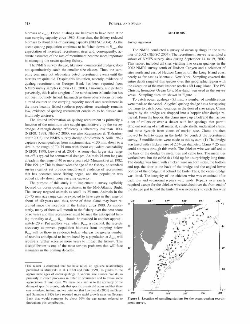
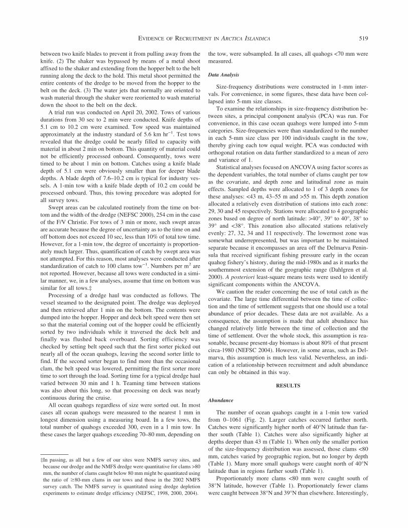
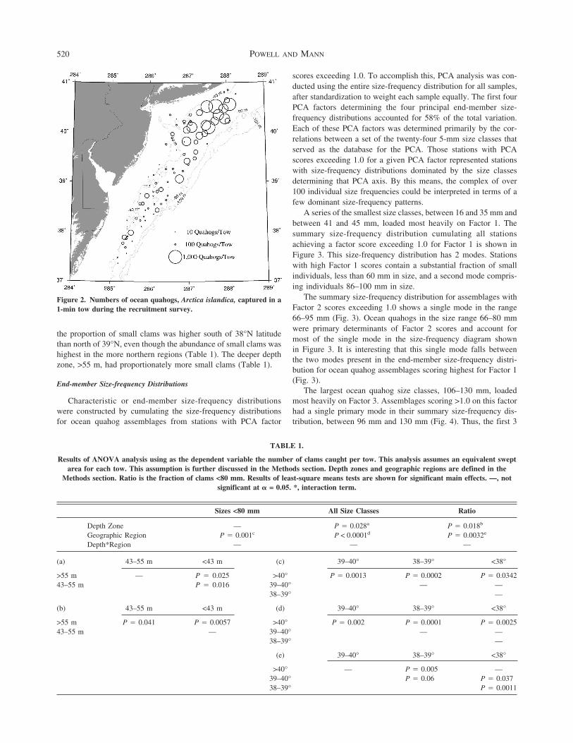
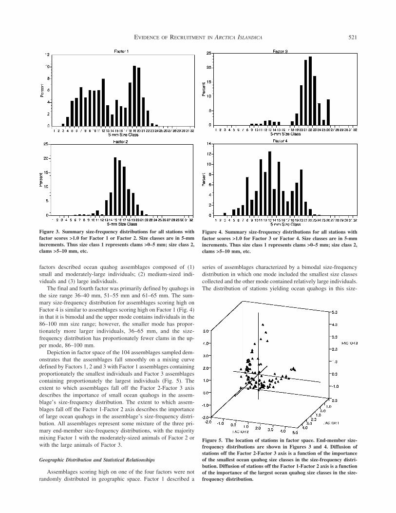
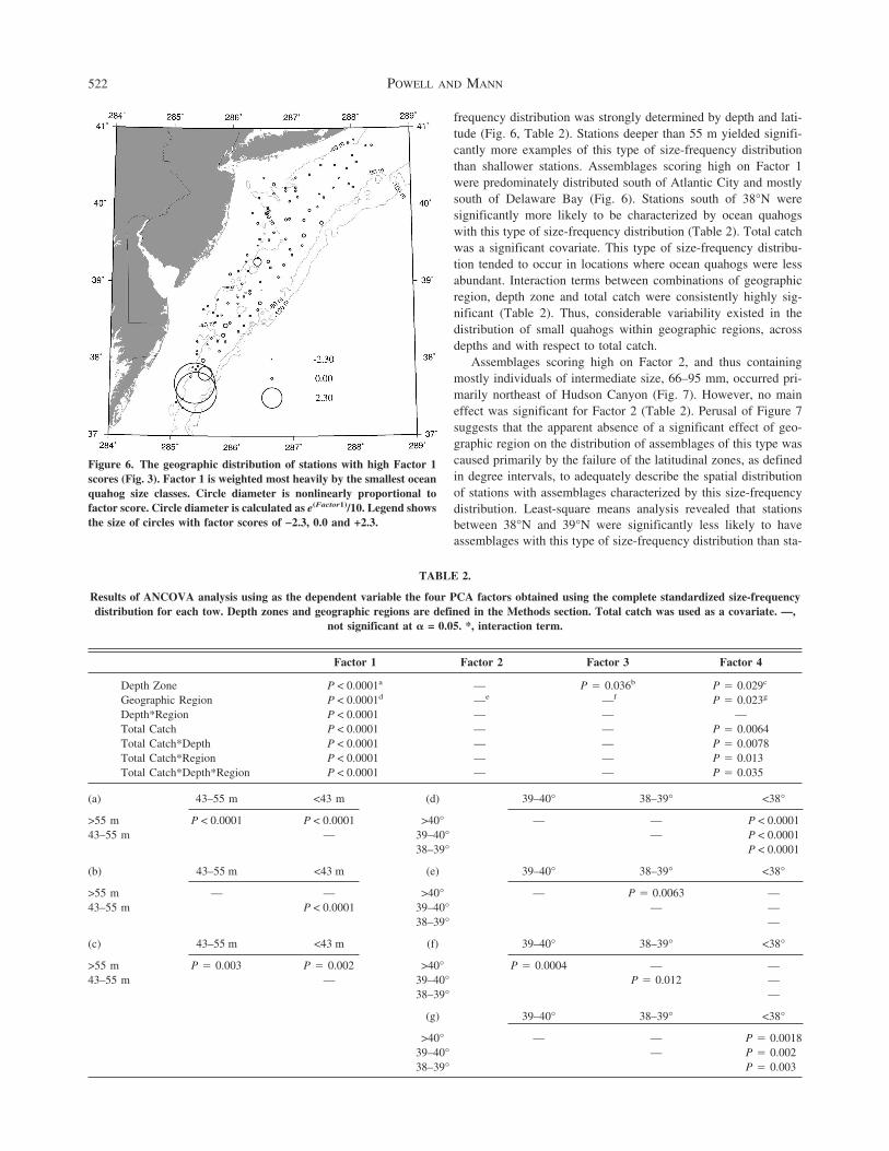
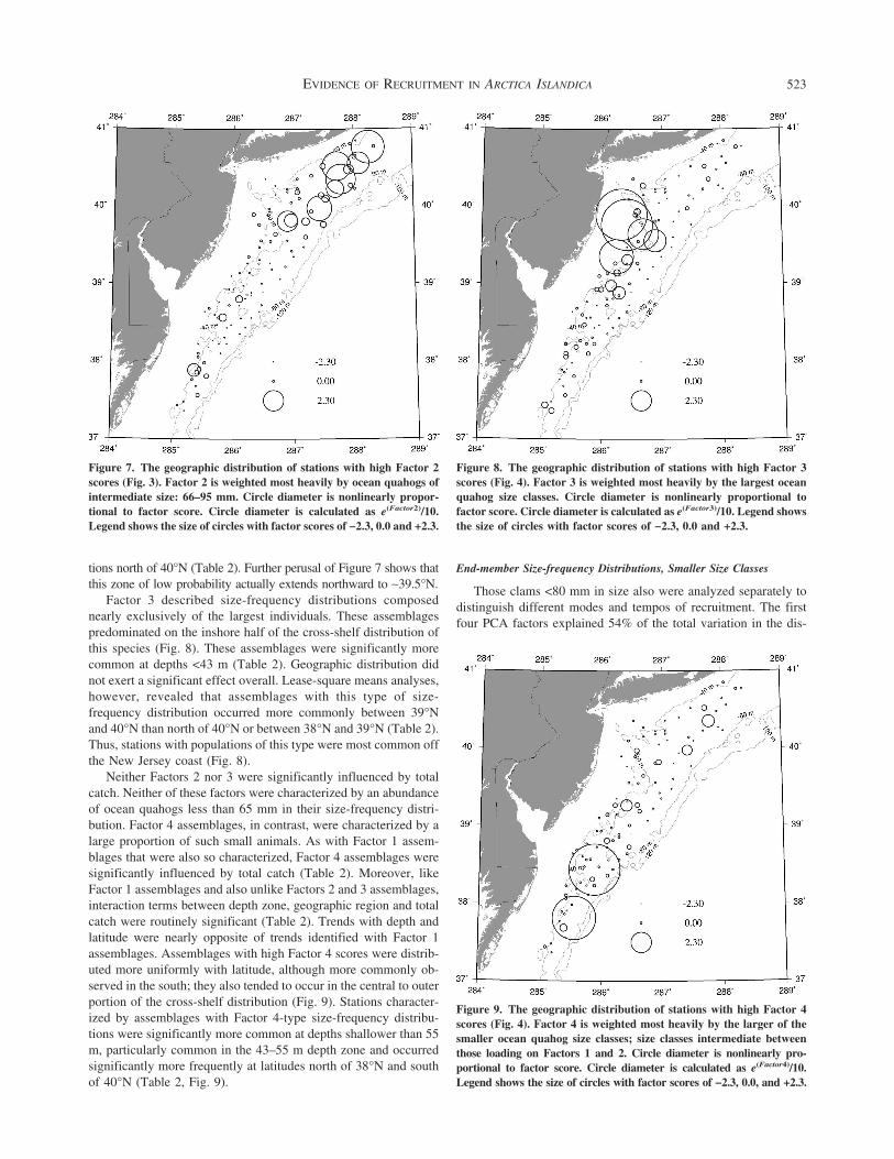
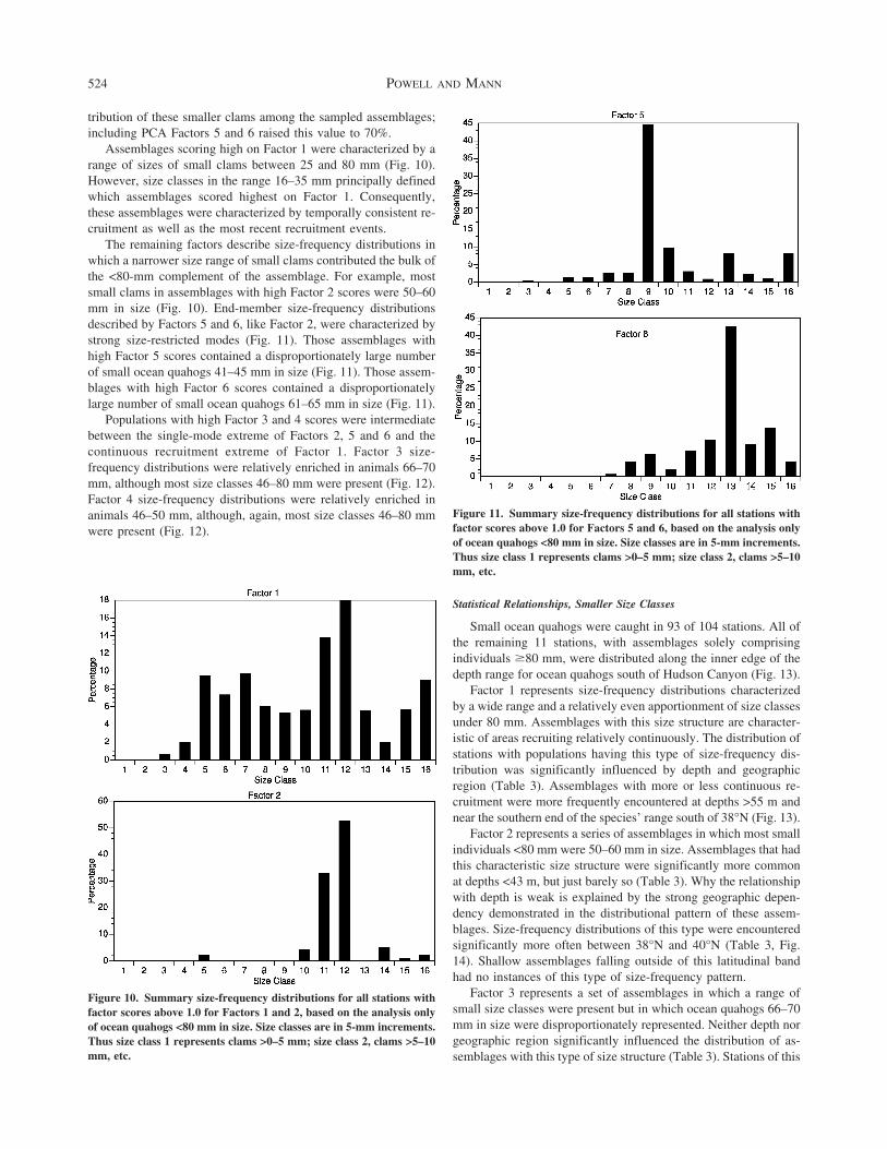
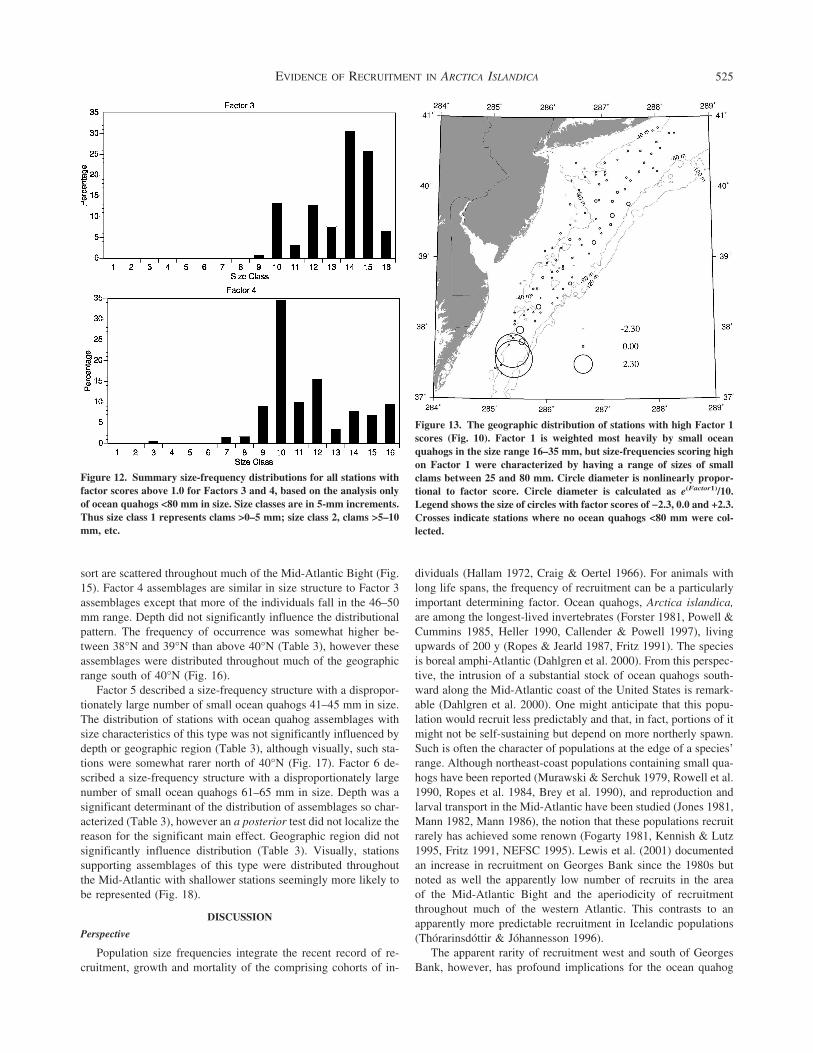
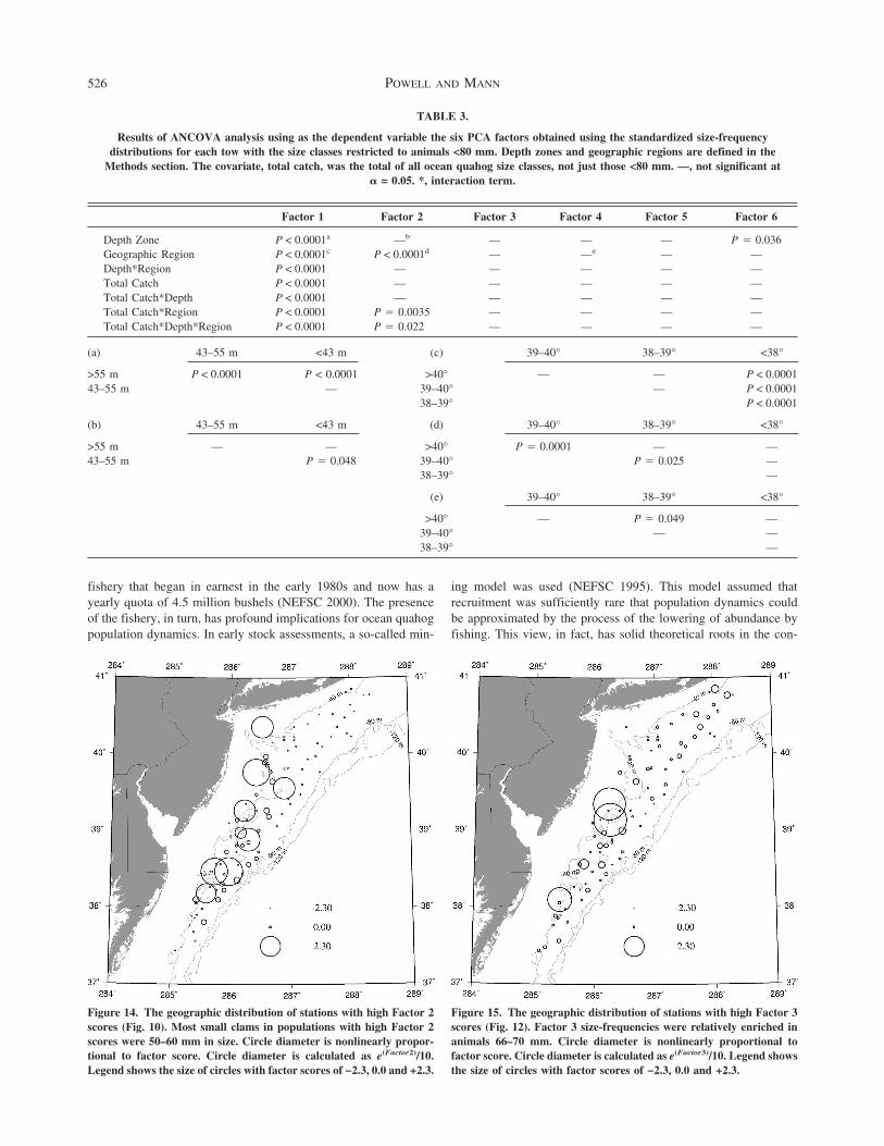
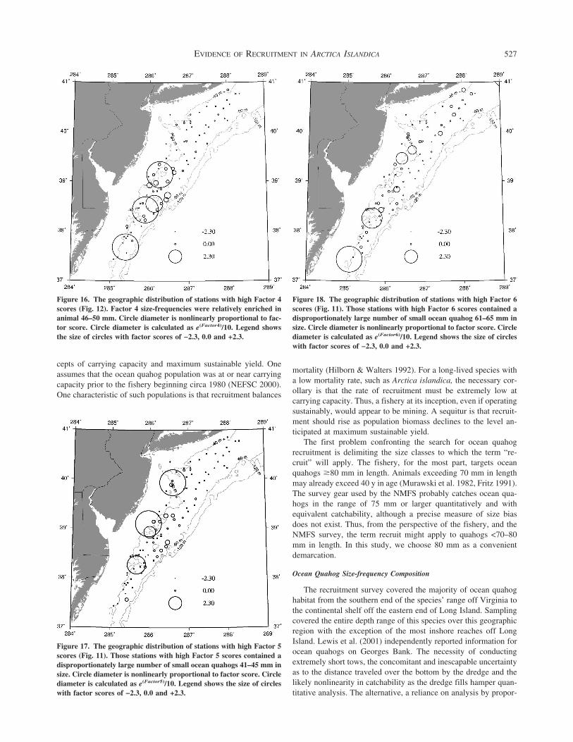
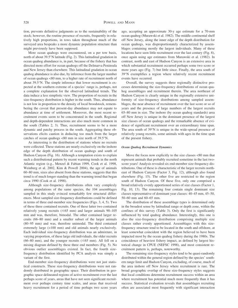