Approximating Piecewise-Smooth Functions

Yaron Lipman David LevinTel-Aviv University

Abstract

We consider the possibility of using locally supported quasi-interpolationoperators for the approximation of univariate non-smooth functions. Insuch a case one usually expects the rate of approximation to be lower thanthat of smooth functions. It is shown in this paper that prior knowledgeof the type of ’singularity’ of the function can be used to regain the fullapproximation power of the quasi-interpolation method. The singularitytypes may include jumps in the derivatives at unknown locations, or evensingularities of the form (x− s)α , with unknown s and α . The new approx-imation strategy includes singularity detection and high-order evaluationof the singularity parameters, such as the above s and α . Using the ac-quired singularity structure, a correction of the primary quasi-interpolationapproximation is computed, yielding the final high-order approximation.The procedure is local, and the method is also applicable to a non-uniformdata-point distribution. The paper includes some examples illustrating thehigh performance of the suggested method, supported by an analysis prov-ing the approximation rates in some of the interesting cases.

1 Introduction

High-quality approximations of piecewise-smooth functions from a discrete setof function values is a challenging problem with many applications in fieldssuch as numerical solutions of PDEs, image analysis and geometric model-ing. A prominent approach to the problem is the so-called essentially non-oscillatory (ENO) and subcell resolution (SR) schemes introduced by Harten[9]. The ENO scheme constructs a piecewise-polynomial interpolant on a uni-form grid which, loosely speaking, uses the smoothest consecutive data points

1

2

in the vicinity of each data cell. The SR technique approximate the singularitylocation by intersecting two polynomials each from another side of the sus-pected singularity cell. In the spirit of ENO-SR many interesting works havebeen written using this simple but powerful idea. Recently, Arandifa et al.[1]gave a rigorous treatment to a variation of the technique, proving the expectedapproximation power on piecewise-smooth data. Archibald et al.[2, 3] haveintroduced the a polynomial annihilation technique for locating the cell whichcontains the singularity. A closely related problem is the removal of Gibbs phe-nomenon in the approximation of piecewise smooth functions. This problemis investigated in a series of papers by Gottlieb and Shu [8]. The methods sug-gested by Gottlieb and Shu are global in nature, using Fourier data informa-tion. These methods are also applicable for uniformly sampled function data,and recently even extended to non-uniform data by Gelb [7]. For a comprehen-sive review of these methods and recent developments see [11]. The methodpresented here relies upon local approximation tools, and thus the singularitydetection algorithm is essentially local, similar to the ENO-SR scheme.

Let g be a real function on [a,b], and let X = {xi}N1 ⊂ [a,b] be a set of data

points, xi < xi+1. We assume that g ∈ PCm+1[a,b] ,where PCm+1[a,b] denotes thefunction space of Cm[a,b] functions with a piecewise continuous m + 1 deriva-tive. Consider approximations to g by quasi-interpolation operators of the type

Qg(x) =N

∑i=1

qi(x)g(xi), (1)

where {qi}Ni=1 are compactly supported functions, qi ∈Cµ [a,b], satisfying a poly-

nomial reproduction property:

Qp = p, p ∈Πm, (2)

where Πm is the polynomial space of degree equal to or smaller than m. Suchoperators are very useful in achieving efficient approximations to smooth func-tions. Namely, let h, the separation distance, be the size of the largest open in-terval J ⊂ [a,b] such that J∩X = /0, and let us assume that supp{qi} = O(h), i =1, ...,N. Then, if the quasi-interpolation operator Q has a bounded Lebesqueconstant, ∑

Ni=1 |qi(x)| ≤C, it follows that

g(x)−Qg(x) = O(hm+1), x ∈ [a,b]. (3)

In this paper we give as examples quasi-interpolation by splines [6] and bymoving least-squares approximations [12].

3

The aim of this paper is to present a simple framework for enhancing suchoperators to well approximate piecewise-smooth functions. In particular wewish to obtain the same approximation order as in approximating smooth data,and furthermore, we would like the singular points in the approximant to begood approximations to the singular points of the approximated function.

2 Quasi-interpolation of piecewise-smooth functions

We consider piecewise-smooth functions f ∈ PCm+1[a,b]\{s}, s ∈ (a,b), whichare PCm+1 smooth except for a single point x = s. We assume that the singu-larity type is known, but its parameters, such as the singularity location andmagnitude, are unknown. Throughout the paper we deal with jump singulari-ties of the derivatives of f , but the discussion can easily be adapted to differentsingularity types. For instance, we also present an example with singularitiesof the type (x− s)α

+, α ∈R+ where (x)+ = x when x≥ 0 and (x)+ = 0 otherwise.Note that in this example the bαc+ 1 derivative limit from the right of s is notfinite.

We thus assume that f can be written as follows:

f (x) = g(x)+ r(x), (4)

where g(x) ∈ PCm+1[a,b], and

r(x) =m

∑j=0

∆ j

j!(x− s) j

+ . (5)

We note that∆ j = f ( j)(s+)− f ( j)(s−).

The error in the quasi-interpolation approximation to f , using data valuesat the points X , can be written as

E f (x) = f (x)−Q f (x) = g(x)−N

∑i=1

qi(x)g(xi)+ r(x)−N

∑i=1

qi(x)r(xi) = Eg(x)+Er(x),

where Eg(x),Er(x) denote the error functions of approximating g(x),r(x) usingQ, respectively.

We assume the quasi-interpolation operator Q has a bounded Lebesqueconstant and hence the expected O(hm+1) approximation order is realized for

4

smooth functions. Therefore, |Eg(x)| = O(hm+1), where h is the fill-distance ofthe data X as defined above, and the deterioration of the approximation is la-tent within the term Er(x).

If the singularity model (type) is known, then Er(x) is known analytically.In our case, assuming r is of the form (5), we have

Er(x) =m

∑j=0

∆ j

j!H j(x;s), (6)

where

H j(x;s) = (x− s) j+−

N

∑i=1

qi(x)(xi− s) j+. (7)

Hence, Er(x) = Er(x;s, ∆̄) is a simple known function of the singularity param-eters s and ∆̄ = {∆ j}m

j=0. Also in our hands, are the values {E f (xi)}, and accord-ing to the above observations

Er(xi) = E f (xi)+O(hm+1) . (8)

Therefore, the general idea for enhancing the quasi-interpolating approx-imation operator is by fitting a function of the form (6) to the actual errors{E f (xi)} in the quasi-interpolation approximation. As we argue below, thefunction Er(x) is of finite support of size O(h). Furthermore, the operator E

annihilates certain polynomials, and this leads to natural orthogonality rela-tions, with respect to the standard inner product. In order to take advantageof these properties we shall use the standard least-squares fitting. We expectthat using other norms will give similar results. The overall procedure is thusas follows: First, we find approximations s∗ and ∆̄∗ = {∆∗j}m

j=0 to the singularityparameters s and ∆̄ by a least-squares fitting:

(s∗, ∆̄∗) := argmins′,∆̄′

N

∑j=1

{E f (x j)−Er(x j;s′, ∆̄′)

}2 (9)

Next, we correct the original quasi-interpolant, and define the new approxima-tion to f as

Q̄ f (x) = Q f (x)+Er(x;s∗, ∆̄∗). (10)

Remark 2.1 The least-squares fitting problem (9) leads to a system of equations whichis linear in the unknowns ∆̄∗ and algebraic (polynomial) in s∗.

5

Remark 2.2 The approximation Q̄ f is piecewise Cµ , with possible jump discontinu-ities in the derivatives at s∗. It is easy to verify that if g ∈ Πm and r is of the form (5),then

Q̄(g+ r) = g+ r. (11)

Note that the above reproduction property does not automatically provide an O(hm+1)approximation order, since the overall process is non-linear.

Remark 2.3 The functions H j(x;s) are of finite support of size O(h). This followsfrom the definition of H j(x;s) and the fact that Q reproduce polynomials of degree lessor equal to m. This consequently implies that the correction term Er(x;s∗, ∆̄∗) is offinite support of size O(h).

In the following theorem we summarize the main properties of the newapproximant Q̄ f (x). For the sake of briefness and clarity we assume that thepoints xi are equidistant, that is, xi = a + ih, i = 0, ...,N, h = b−a

N and that thequasi-interpolation basis functions are all shifts of one function:

qi(x) = q( x

h− i)

,

where supp{q(Z)} = [−e,e]∩Z, e = 2,3, .... In fact, to achieve polynomial re-production over the whole interval [a,b], one should use some special basisfunctions near the end points of the interval. However, since we assume thatthe singularity of f is at a fixed point s ∈ (a,b), and since we consider asymp-totics as h→ 0, and q(·) is of a finite support, it is enough to consider a shiftinvariant basis. In order to retain the polynomial reproduction over [a,b], andmaintain the simplicity of a shift invariant basis, we augment the point set withe extra points on each side, that is, xi = a+ ih, i =−e, ...,N + e.

Theorem 2.1 Assume Q is a quasi-interpolation operator reproducing polynomialsin Πm. Let f be a continuous function in [a,b] of the form (4) with ∆1 6= 0. Theapproximant Q̄ f (x) defined above satisfies the following properties:

1. Q̄ f has the same smoothness as Q f except for the point s∗ where it has the sin-gularity type of the singularity model.

2. |s− s∗|= O(hm+1) and |∆ j−∆∗j |= O(hm+1− j), j = 1,2, ...,m.

3. Q̄ f has full approximation order, that is,

| f (x)− Q̄ f (x)|= O(hm+1).

6

Proof. Claim 1 follows directly from the definition of the correction termE(x;s∗, ∆̄∗). In order to prove claims 2 and 3, we first note that the parameterss∗ and ∆∗ minimizing (9) certainly satisfy

N

∑j=0

{E f (x j)−Er(x j;s∗, ∆̄∗)

}2 ≤N

∑j=0

{E f (x j)−Er(x j;s, ∆̄)

}2.

Existence of a minimizer s∗ is proved in Appendix A. Next, it follows fromRemark 2.3 that there is a fixed number (independent of h) of indices j suchthat Er(x j;s∗, ∆̄∗) 6= 0 or Er(x j;s, ∆̄) 6= 0. Combining this with the fact that

E f (x j)−Er(x j;s, ∆̄) = O(hm+1) ,

we getEr(x j;s, ∆̄)−Er(x j;s∗, ∆̄∗) = O(hm+1). (12)

Therefore, we can conclude that the corrected approximation gives the rightapproximation order at the data points:

| f (x j)− Q̄ f (x j)|= O(hm+1) .

For the proof of claim 3 we shall use (12) in order to show that

Er(x;s, ∆̄)−Er(x;s∗, ∆̄∗) = O(hm+1) , ∀x ∈ [a,b] .

This part of the proof is less obvious, and is rather lengthy:

From the definitions we have that

Er(x;s, ∆̄)−Er(x;s∗, ∆̄∗) =

∑mj=1

∆ jj!

[(x− s) j

+−∑i qi(x)(xi− s) j+

]−∑

mj=1

∆∗jj!

[(x− s∗) j

+−∑i qi(x)(xi− s∗) j+

](13)

Next, note that

(x− s) j+−∑

iqi(x)(xi− s) j

+ =−(x− s) j−+∑

iqi(x)(xi− s) j

−, 0≤ j ≤ m, (14)

and similarly for s∗. These identities can be understood via the polynomialreproduction property of Q. Let us define the following polynomials of degreem:

p(x) =m

∑j=1

∆ j

j!(x− s) j , p∗(x) =

m

∑j=1

∆∗jj!

(x− s∗) j. (15)

7

W.l.o.g. we assume that s≤ s∗, otherwise the following can be adapted accord-ingly. Using (13) and (14) we get:

Er(x;s, ∆̄)−Er(x;s∗, ∆̄∗) = ∑i

qi(x)

Λ1

i x < s

Λ2i s≤ x < s∗

Λ3i s∗ ≤ x

, (16)

where

Λ1i =

0 xi < s

−p(xi) s≤ xi < s∗

p∗(xi)− p(xi) s∗ ≤ xi

Λ2i =

p(xi) xi < s

0 s≤ xi < s∗

p∗(xi) s∗ ≤ xi

(17)

Λ3i =

p(xi)− p∗(xi) xi < s

−p∗(xi) s≤ xi < s∗

0 s∗ ≤ xi

, i =−M− e, ...,N + e

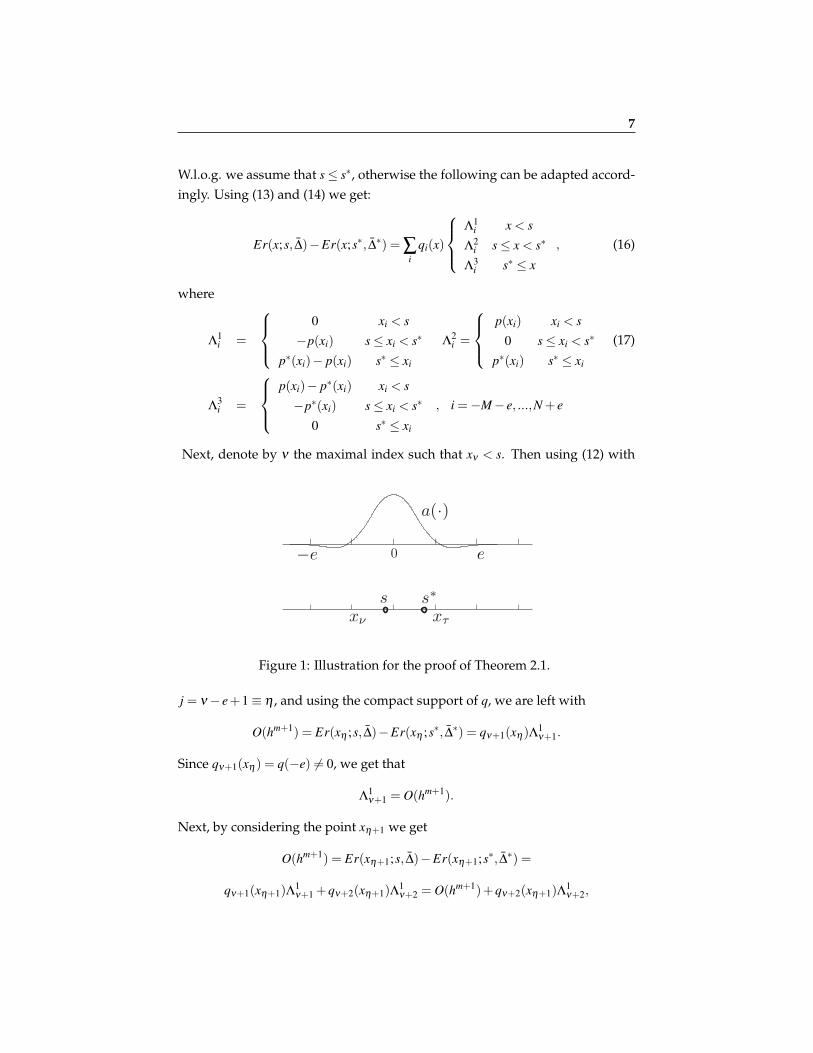
Next, denote by ν the maximal index such that xν < s. Then using (12) with

s s∗

xτxν

0 e−e

a(·)

Figure 1: Illustration for the proof of Theorem 2.1.

j = ν− e+1≡ η , and using the compact support of q, we are left with

O(hm+1) = Er(xη ;s, ∆̄)−Er(xη ;s∗, ∆̄∗) = qν+1(xη)Λ1ν+1.

Since qν+1(xη) = q(−e) 6= 0, we get that

Λ1ν+1 = O(hm+1).

Next, by considering the point xη+1 we get

O(hm+1) = Er(xη+1;s, ∆̄)−Er(xη+1;s∗, ∆̄∗) =

qν+1(xη+1)Λ1ν+1 +qν+2(xη+1)Λ1

ν+2 = O(hm+1)+qν+2(xη+1)Λ1ν+2,

8

and since qν+2(xη+1) = q(−e) 6= 0 we have

Λ1ν+2 = O(hm+1).

We can continue in the same manner showing

Λ1i = O(hm+1) , ν +1≤ i≤ ν + e. (18)

In a similar manner we also get

Λ3i = O(hm+1) , τ−1≥ i≥ τ− e, (19)

where τ is the minimal index such that s∗ ≤ xτ . Next, let us show that for asmall enough h there is at most one mesh point between xν to xτ , that is, ei-ther τ = ν + 1 or τ = ν + 2. Otherwise, if xν+2 < s∗, since e ≥ 2, then p(xν+2) =−Λ1

ν+2 = O(hm+1). But since ∆1 6= 0, and xν+2− s > h, we have p(xν+2) = θ(h)which yields a contradiction for small enough h. So in the last part of the proof,we deal with each of the two possible cases: τ = ν +1 and τ = ν +2.

Case 1: If τ = ν +1, in this case we have

Λ3i = p(xi)− p∗(xi) = O(hm+1) , i = τ− e, ...,ν , (20)

Λ1i = −p(xi)+ p∗(xi) = O(hm+1) , i = τ, ...,ν + e,

that is, we have 2e points where the polynomial p− p∗ has an O(hm+1) value.Since p− p∗ is a polynomial of degree less than or equal to m and necessarily2e≥ m+1, we get that for x ∈ [xτ−e−2,xν+e+2]

p(x)− p∗(x) = O(hm+1). (21)

This has several consequences: First, setting x = s∗ we get

p(s∗) = O(hm+1),

hence, since ∆1 6= 0, we get that |s− s∗| = O(hm+1). Secondly, for x < s (s∗ ≤ x),we see that all relevant Λ1

i (Λ3i ) are O(hm+1) and therefore we have that

Er(x;s, ∆̄)−Er(x;s∗, ∆̄∗) = O(hm+1) , x < s,s∗ ≤ x.

Finally, for s≤ x < s∗, Er(x;s, ∆̄)−Er(x;s∗, ∆̄∗) =

ν+e+2

∑i=τ−e−2

qi(x)Λ2i =

ν+e+2

∑i=τ−e−1

qi(x)p(xi)+O(hm+1) = p(x)+O(hm+1) = O(hm+1),

9

where the first equality uses (17) and (21) and the second equality is due topolynomial reproduction.

Case 2: If τ = ν + 2. In this case we only have 2e− 1 points (i = τ − e, ...,ν + e)where p− p∗ is O(hm+1). In order to obtain such a relation at yet another point,we use the extra information we have, namely,

p(xν+1) =−Λ1ν+1 = O(hm+1). (22)

Using (17), (18), (19) we have

O(hm+1) = Er(xν+1;s, ∆̄)−Er(xν+1;s∗, ∆̄∗) =ν+e+1

∑i=τ−e−1

qi(xν+1)Λ2i =

ν+e+1

∑i=τ−e−1

qi(xν+1)p(xi)+qν+e+1(xν+1)(p∗(xν+e+1)− p(xν+e+1))+O(hm+1) =

p(xν+1)+qν+e+1(xν+1)(p∗(xν+e+1)− p(xν+e+1))+O(hm+1).

Observing that qν+e+1(xν+1) = q(−e) 6= 0 and using (22), we get

p∗(xν+e+1)− p(xν+e+1) = O(hm+1),

and we can continue as in the first case.Finally, let us prove |∆ j −∆∗j | = O(hm+1− j). First note that we have that thereexist 2e consecutive points xi1 , ...,xi2e ∈ X such that p(xi j)− p∗(xi j) = O(hm+1).Next let us write p− p∗ in the Lagrange basis

p(x)− p∗(x) =2e

∑j=1

(p(xi j)− p∗(xi j)

)L j(x),

where the functions L j(x) =∏χ 6= j(x−xiχ )

∏χ 6= j(xi j−xiχ ) , j = 1, ..,2e form the Lagrange basis.

SincedJ

dxJ

∣∣∣∣x∈[min{xi j },max{xi j }]

L j(x) = O(h−J),

we get thatdJ

dxJ

∣∣∣∣x=s∗

(p(x)− p∗(x)) = O(hm+1−J).

On the other hand, for any J = 1, ...,m, differentiating p(x)− p∗(x) J times andsubstitute x = s∗ we have

dJ

dxJ

∣∣∣∣x=s∗

(p(x)− p∗(x)) = ∆J−∆∗J +

m

∑j=J+1

∆ j

( j− J)!(s∗− s) j−J .

2.1 Algorithm 10

Since |s− s∗|= O(hm+1) the previous two equations imply that

|∆∗J−∆J |= O(hm+1−J).

�

2.1 Algorithm

From a practical point of view, we suggest two algorithms for alleviating quasi-interpolants Q to accommodate piecewise-smooth data with known singular-ity family type Q̄: First, in the case of jump in the first derivative we providea closed-form formula for locating the singularity and approximating the sin-gularity parameters. The algorithm and its analysis are provided in Section 3.The computational complexity of the algorithm in this case is O(N) (where N isthe number of data points).

Second, in the general case, the algorithm is as follows. First, an initial(rough) guess s0 to the singularity location s is constructed. This can be donein several ways. We have used for example

s0 = argmins′

∑j|E f (x j)||x j− s′|2.

This boils down to the centroid of the error E f . Another option could be to usethe ENO scheme for locating a cell or few cells that might contain the singu-larity. The initial guess provides us with |s0− s| = O(h) approximation of thesingularity location and its computational complexity is O(N), where again N isthe number of data points. It Should be noted that in the case that h is not smallenough, the algorithm may provide an erroneous approximation, especially incases of detecting high order singularities. In the second step a minimizationof the functional (9) is done by minimizing the functional as a (rational) func-tion of s′ in a constant number of intervals adjacent to the initial guess s0. Thatis, denote by ∆̄′ = ∆̄′(s′) the minimizer of (9) with respect to a fixed s′, then thefunctional

N

∑j=1

{E f (x j)−Er(x j;s′, ∆̄′(s′))

}2,

is minimized with respect to s′ in the above mentioned intervals. The compu-tational complexity of the second step is constant, that is, independent of N.This follows from the fact that the support of Er contains only a fixed numberof data points (assuming a quasi-uniform data set).

11

3 A closed form solution for a special case

As explained in Remark 2.1, the least-squares fitting problem (9) leads to asystem of equations which is linear in the unknowns ∆̄∗ and algebraic (polyno-mial) in s∗. However, in the special case where f has jump discontinuities at s

only in its value and its first derivative we can present a closed form solutionof (9). In this case we have also observed some superconvergence of the ap-proximation s∗ to s, which we prove below. This case is a particular instance offunctions which are linear combinations of smooth functions and spline func-tions.

In that case (6) reduces to

Er(x;s′, ∆̄′) = ∆′0H0(x;s′)+∆

′1H1(x;s′), (23)

Assume s ∈ (xk,xk+1], in such a case the sum to be minimized in (9) becomes

∑Nj=1{

E f (x j)−∆′0[(x j− s′)0

+−∑Ni=1 qi(x j)(xi− s′)0

+]

−∆′1[(x j− s′)+−∑

Ni=1 qi(x j)(xi− s′)+

]}2 =

∑Nj=1{

E f (x j)−∆′0[(x j− xk+1)0

+−∑i≥k+1 qi(x j)]

−∆′1[(x j− xk+1)0

+(x j− s′)−∑i≥k+1 qi(x j)(xi− s′)]}2

(24)

After rearranging we get

∑Nj=1{

E f (x j)− (∆′1s′−∆′0)[−(x j− xk+1)0

+ +∑i≥k+1 qi(x j)]

−∆′1[(x j− xk+1)0

+x j−∑i≥k+1 qi(x j)xi]}2

.(25)

And the functional is quadratic in the variables (∆′1s′−∆′0) and ∆′1.

Obviously, the minimizer in this case is not unique. Therefore, let us con-sider the case where ∆0 = 0, that is, f is continuous. In that case (25) reduces toa 2×2 linear system in the variables

∆̃′1 := ∆

′1 , s̃′ := ∆

′1s′.

Denote the functions

φk(x) = x(x− xk+1)0+−∑i≥k+1 qi(x)xi,

ψk(x) = −(x− xk+1)0+ +∑i≥k+1 qi(x).

(26)

3.1 Approximation order analysis 12

By the polynomial reproduction property of the quasi-interpolation operator itfollows that both φk and ψk are of compact support of size O(h). Then equation(25) turns into

N

∑j=1

{E f (x j)− s̃′ψk(x j)− ∆̃

′1φk(x j)

}2. (27)

Let us define the matrix A = (ψ , φ) where φ ,ψ are column vectors defined by

φ j = φk(x j) , ψ j = ψk(x j). (28)

Then, the normal equations for system (27) is:

AtA

(s̃′

∆̃′1

)= At (E f (x1), ...,E f (xN))t . (29)

Hence, the algorithm for calculating the approximations s∗,∆∗1 to the truesingularity parameters s,∆1 can be described concisely as follows: for each in-terval [xi,xi+1], minimize the functional in (9) constrained to the interval [xi,xi+1],that is, solve (29): if s′ = s̃′/∆̃′1 ∈ [xi,xi+1] it is the minimum of (9) in that inter-val. Otherwise, evaluate the functional at the ends s′ = xi,∆

′1 = ∆′1(s

′) and thesame for xi+1. The minimum of the functional on this interval will be attainedat one of the ends. Finally denote by s∗,∆∗1 the values which yielded the globalminimum of the functional (9).

Note that we have used the symbol ∆′(s′) to denote, as remarked in (2.1),that fixing s′ in functional (9) results in a linear system for ∆. In Appendix Athis system is proved to be non-singular.

3.1 Approximation order analysis

An important virtue of the above method is that, by using m−th degree quasi-approximation operator, we get an O(h2(m+B)−1) approximation order to thelocation of the singular point, where m + B is the maximal degree of the poly-nomials reproduced by the quasi-interpolation operator at the nodes. In thissection we provide the analysis of this approximation order. Regarding differ-ent types of singularities (not only jump in the first derivative) we have alsoobserved some superconvergence properties; in Section 5 we present some nu-merical experiments demonstrating this phenomenon and compare it to thesubcell resolution method of similar degree.

3.1 Approximation order analysis 13

We return to the settings of equidistant point xi = a + ih, −e ≤ i ≤ N + e,h = b−a

N , and to basis functions qi(·) which are shifted versions of a “motherbasis function” q(x), that is,

qi(x) = q( x

h− i)

.

Let us set k such that s ∈ [xk,xk+1]. The normal equations (29) which aresolved for the s̃∗, ∆̃∗1 are

AtA

(s̃∗

∆̃∗1

)= AtE f = At

(A

(s̃

∆̃1

)+ ε

)= AtA

(s̃

∆̃1

)+At

ε, (30)

where ε stands for the errors in approximating the smooth part of f , that isε j = Eg(x j), and s̃ = s ·∆1 , ∆̃1 = ∆1 where s,∆1 are the true singularity positionand the jump in the first derivative, respectively.

In order to prove the desired approximation result |s∗− s|= O(h2(m+B)−1), itis enough to prove

|s̃∗− s̃|= O(h2(m+B)−1) , |∆̃∗1− ∆̃1|= O(h2(m+B−1)).

By (30) we have (s̃∗− s̃

∆̃∗1− ∆̃1

)= (AtA)−1At

ε. (31)

It is quite easy to get a bound of the form

‖(AtA)−1At‖= O(h−r),

with some r > 0 where ‖ · ‖ = supv6=0‖·v‖∞‖v‖∞ , ‖v‖∞ = maxi{|vi|} . And since ε =

O(hm+1) we will generally only get

‖(AtA)−1Atε‖= O(h−r+m+1).

The key property which yields the higher approximation order is that the vec-tors φ and ψ are orthogonal to some polynomial vectors X ` = {x`

i }Ni=0, ` =

0,1, ..., `′. Then, if ε is smooth, it can be well approximated by polynomials,and therefore it will follow that ‖Atε‖ decreases faster than ‖At‖‖ε‖ as h→ 0.

In the following we prove the main ingredients of the superconvergenceresult.

3.1 Approximation order analysis 14

Lemma 3.1 Let B ∈N+ such that Q reproduce polynomials of maximal degree m+B

on the nodes X ; then we have the following orthogonality relations:

〈φ ,X `〉= 0 ` = 0,1, ...,m+B−2,

〈ψ,X `〉= 0 ` = 0,1, ...,m+B−1.

Proof. First denote the operator T by

T (ξ ) j = ξ j−∑i

qi(x j)ξi, (32)

then the vectors φ ,ψ (28) can be written as follows:

φ = T (r1) , ψ = T (r0),

where r0j = (x j− xk+1)0

+ and r1j = x j(x j− xk+1)0

+. Since T has finite support onR∞ and T ({p( j)}) = 0 for all p ∈Πm+B(R) it can be written as

T = R∆m+B+1 = ∆

m+B+1R,

where ∆ is the forward difference operator, that is, (∆ξ ) j = ξ j+1 − ξ j and R

has compact support. Next we make use of the summation by parts (S.B.P.)formula:

N

∑i=−M

fi∆gi = [( f )·(g)·]N+1−M −

N

∑i=−M

gi+1∆ fi. (33)

Using (33) m + B− b times, b = 0,1, and since (∆m+B+1−ν rb) j = 0, j = 0,N + ν

for all ν ≤m+B−b plus the fact that ∆m+B−b annihilates polynomial sequences{p( j)} for p ∈Πm+B−1−b(R) the lemma is proved. �

Lemma 3.2 There exists a matrix Q ∈RN+1×2, such that

1. A can be written as

A = Q

(1 xk+1

0 h

),

where Q j,i 6= 0, i = 1,2 only for some fixed number of indices j around k.

2. QtQ and ‖Qt‖ are independent of h.

Proof. Using the notation of previous lemma,

A

(1 −xk+1

0 1

)=(T (x·− xk+1)0

+,T (x·− xk+1)+)

=

3.1 Approximation order analysis 15

(T (·− (k +1))0

+,T (·− (k +1))+)( 1 0

0 h

).

Therefore

A =(T (·− (k +1))0

+,T (·− (k +1))+)( 1 xk+1

0 h

)≡Q

(1 xk+1

0 h

).

This shows (1). Next, note that T is translation invariant. Indeed, denote by E

the translation operator, that is (EX) j = x j−1, then

T E(·) = ET (·).

Hence, we have that

T (·− (k +1))0+ = T Ek+1(·)0

+ = Ek+1T (·)0+.

And similarlyT (·− (k +1))+ = Ek+1T (·)+.

We therefore see that the column vectors of the matrix Q consist of shiftedversions of the constant (independent of h) vectors

T (·)0+ , T (·)+.

Therefore, the second claim of the lemma is evident. �

Lemma 3.3 The normal matrix AtA ∈R2×2 is invertible and we have

‖(AtA)−1At‖= C1h−1. (34)

Proof. For the first part it is enough to show that the vectors φ ,ψ are linearlyindependent. Using (33) ν = m+B times, we get, as shown in Lemma 3.1,

〈ψ,Xm+B−1〉= 0. (35)

However, we also get

〈φ ,Xm+B−1〉 = (−1)m+B−1 [(R∆r1)·+m+B−1(∆m+B−1Xm+B−1)·]N+1

0 (36)

= (−1)m+B−1hm+B−1(m+B−1)!(R∆r1)N+m+B

= (−1)m+B−1hm+B(m+B−1)!(R(1))N+m+B

6= 0,

3.1 Approximation order analysis 16

where the second equality follows from the fact that ∆r1 equals zero near theleft boundary, and in the last inequality 1 j = 1, R(1)N+m+B = C1 6= 0 since m+B

is the maximal reproduction degree of T on the nodes X . Finally, from (36) and(35) it follows that φ ,ψ are linearly independent. Furthermore, (34) is evidentfrom Lemma 3.2. �

Finally, we can prove the stated approximation order result:

Theorem 3.1 Let f be a function of the form

f (x) = g(x)+∆1(x− s)+,

where g ∈ PC2(m+B). Let Q be a quasi-interpolation operator of order m as defined in(1). Further assume that |s−x j| ≥ chm,x j ∈X for some constant c. Then, the algorithmdescribed in Section 3 results in the approximation

|s∗− s|= O(h2(m+B)−1) ; |∆∗1−∆1|= O(h2(m+B)−1).

Proof. It is enough to prove

|s̃∗− s̃|= O(h2(m+B)−1) , |∆̃∗1− ∆̃1|= O(h2(m+B−1)).

By Theorem 2.1 we have that |s∗− s| = O(hm+1). Combining this with the as-sumption that |s− x j| ≥ chm we get that, for small enough h, s∗ is in the sameinterval as s, that is s∗ ∈ [xk,xk+1]. In this case we have from (31) that

|∆̃1− ∆̃∗1|, |s̃− s̃∗| ≤ ‖(AtA)−1At

ε‖,

where ε = R∆m+B+1g(X). By Lemma 3.1 we have that both φ ,ψ annihilatespolynomials of degree m+B−2, that is

〈φ ,X `〉= 〈ψ,X `〉= 0 , ` = 0,1, ...,m+B−2.

Therefore by expanding g to its Taylor series through order 2(m+B)−1, that isg = gT +O(h2(m+B)), we have that

‖(AtA)−1Atε‖= ‖(AtA)−1AtO(h2(m+B))‖= O(h2(m+B)−1),

where in the last equality we used Lemma 3.3.�

17

4 Noise at isolates data points

The classical approach to detecting and fixing noise at isolated data points [5,4, 10] is based on using the divided difference operator. One assumes the datais corrupted with noise at some data point xk, that is,

f (xi) = g(xi)+ εδ (xi− xk),

where δ (z) equals one if z = 0, and zero otherwise. The method for detectingxk and approximating the value ε is based on observing distinct pattern of theerror

∆m{εδ (xi− xk)}i = ε

(m

i

)(−1)m−i,

This error increases in absolute value as m increases in contrast to the divideddifference of the smooth part g which generally decreases as m increases. Theabove pattern is searched for in the data to locate the corrupted data pointxk, and then a suitable ε∗ ≈ ε is calculated. Finally the input data points arecorrected by subtracting this ε∗ from the detected data point value. We arenot aware of an explicit method for computing ε or any result addressing theapproximation order of this method.

This method is closely related to our approach and can be easily understoodas a particular instance where the singularity model used is a jump at a singledata-point

r(x) = εδ (x− xk).

Since we assume the noise is at one of the data points, we can explicitly checkevery data point x j, and calculate ε∗j to minimize (9). Using the normal equa-tions the minimizer is

ε∗j =

〈E f (X),H(X ;x j)〉〈H(X ;x j),H(X ;x j)〉

,

where{

H(X ;x j)}

i = δ (xi− x j)−qk(xi). Then one uses the j and correspondingε∗j which minimize (9) among all possible data points to rectify the input dataat point x j.

Using similar analysis to Section 3.1 it is easy to prove the following,

Theorem 4.1 Let f be a function of the form

f (x) = g(x)+ εδ (x− xk),

18

where ε ≥ 0 and g ∈ PC2(m+B)+2. Let Q be a quasi-interpolation operator of order m

as defined in (1) which reconstructs polynomials of order m + B at the data points.Then, for small enough h, the above procedure finds xk, and approximates the noiselevel ε to the order O(h2(m+B)+2), that is

|ε∗− ε|= O(h2(m+B)+2).

Proof. For every s′ = x j the functional in (9) becomes

‖E f − ε∗j H j‖2 =

⟨E f −

〈E f ,H j〉〈H j,H j〉

H j,E f −〈E f ,H j〉〈H j,H j〉

H j

⟩,

where we substituted the minimizer ε∗j = 〈E f ,H j〉〈H j ,H j〉 , and H j = H(X ;x j). Using the

fact that E f = Eg+Er = O(hm+1)+ εHk we then get

‖E f − ε∗j H j‖2 = ‖εHk−

〈εHk,H j〉〈H j,H j〉

H j‖2 +O(hm+1),

which for small enough h attains its minimum only for j = k.

After finding xk, the normal equations for (9) are

HtHε∗ = HtE f (X) = HtEg(X)+HtHε,

where H = H(X ;xk). Expanding g to its Taylor series through order 2(m+B)+1,we get, similarly to Theorem 3.1,

HtH(ε∗− ε) = HtHEg(X) = O(h2(m+B)+2),

and since HtH ≥ c > 0 for some c independent of h we get the desired approxi-mation order. �

5 Numerical experiments and concluding remarks

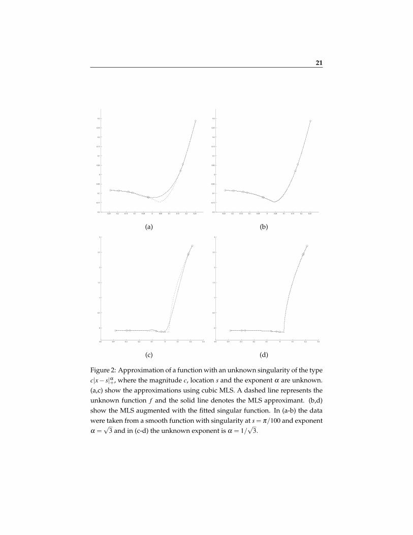
In this section we present a few numerical experiments with the method pre-sented above. First, in Figure 2 we present an example of approximating afunction with the singularity model of the form c|x− s|α+, where c,s,α are un-known. Here, we used cubic Moving Least Squares on irregular nodes asa quasi-interpolation operator Q. Experimentally, for the case of equidistantpoints an approximation order O(h8) to s has been observed.

19

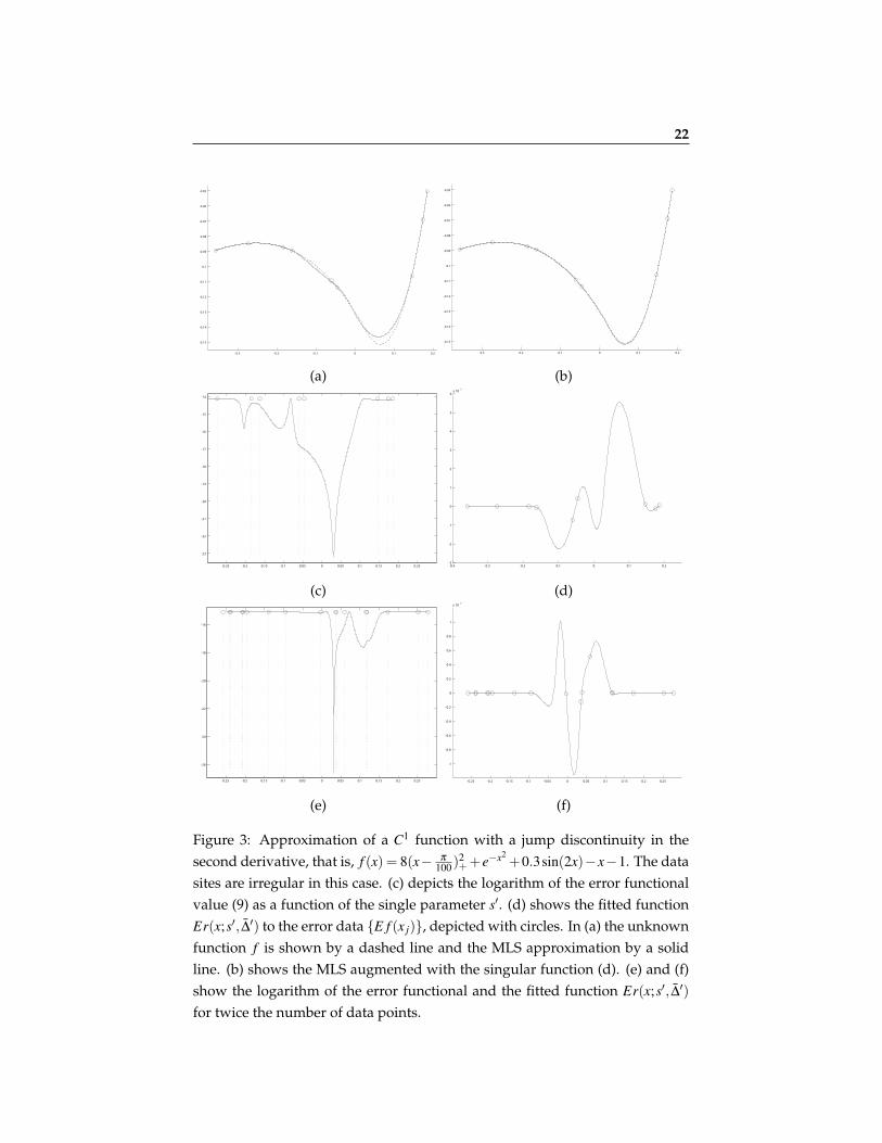
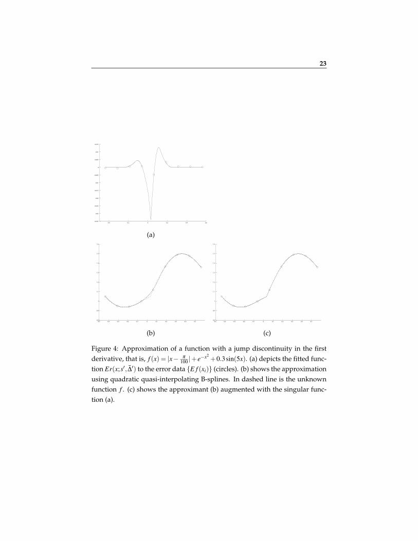
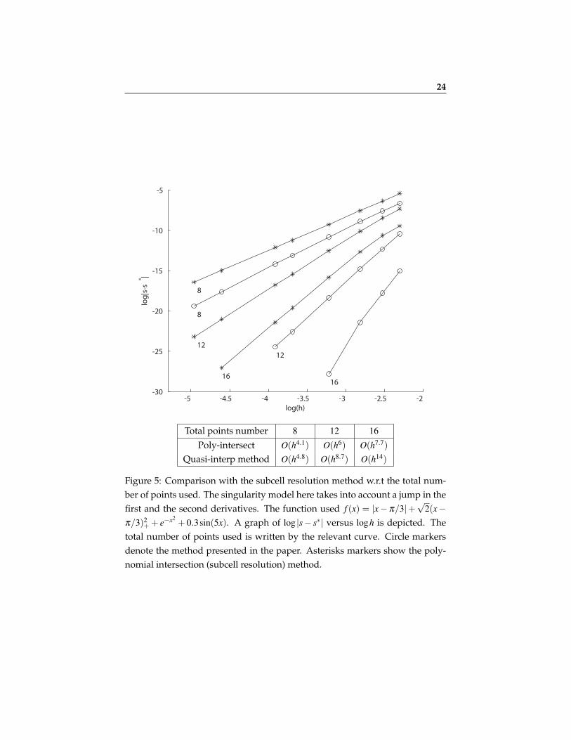
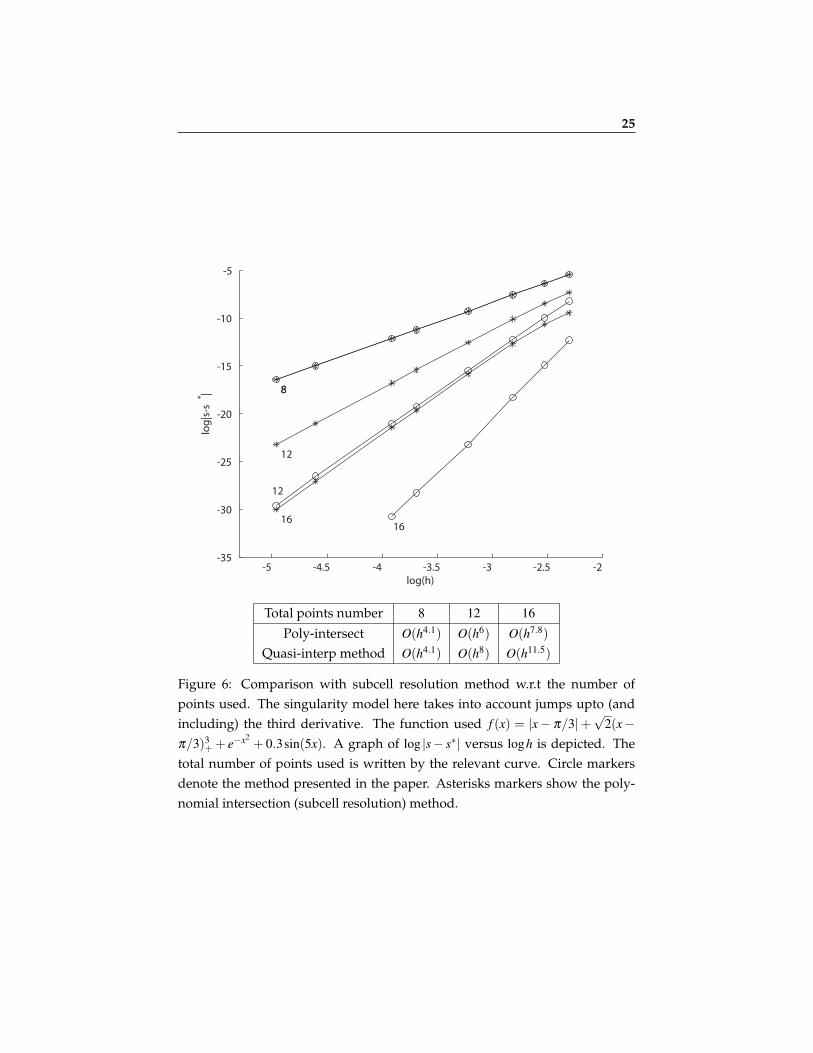
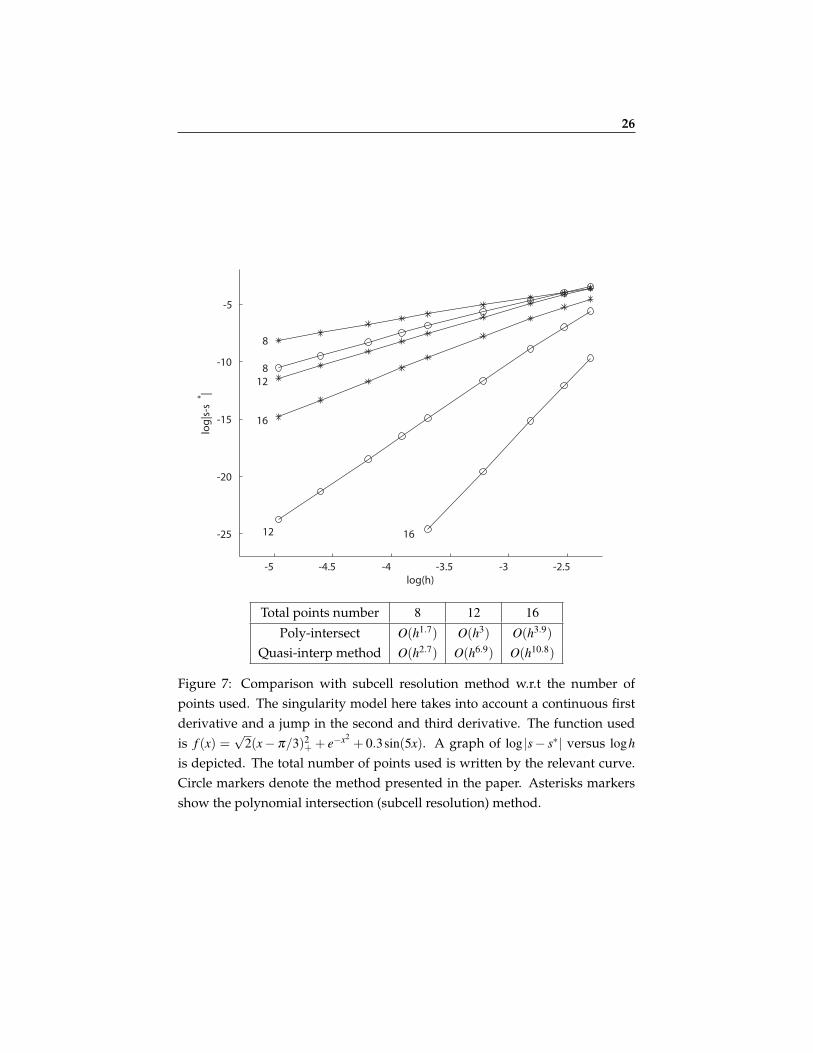
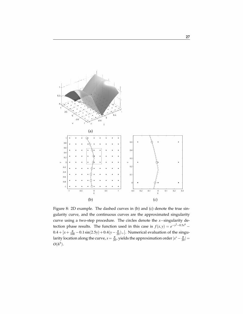
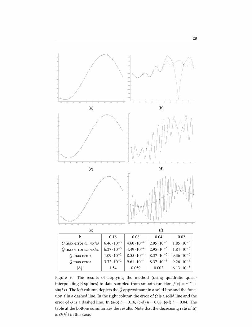
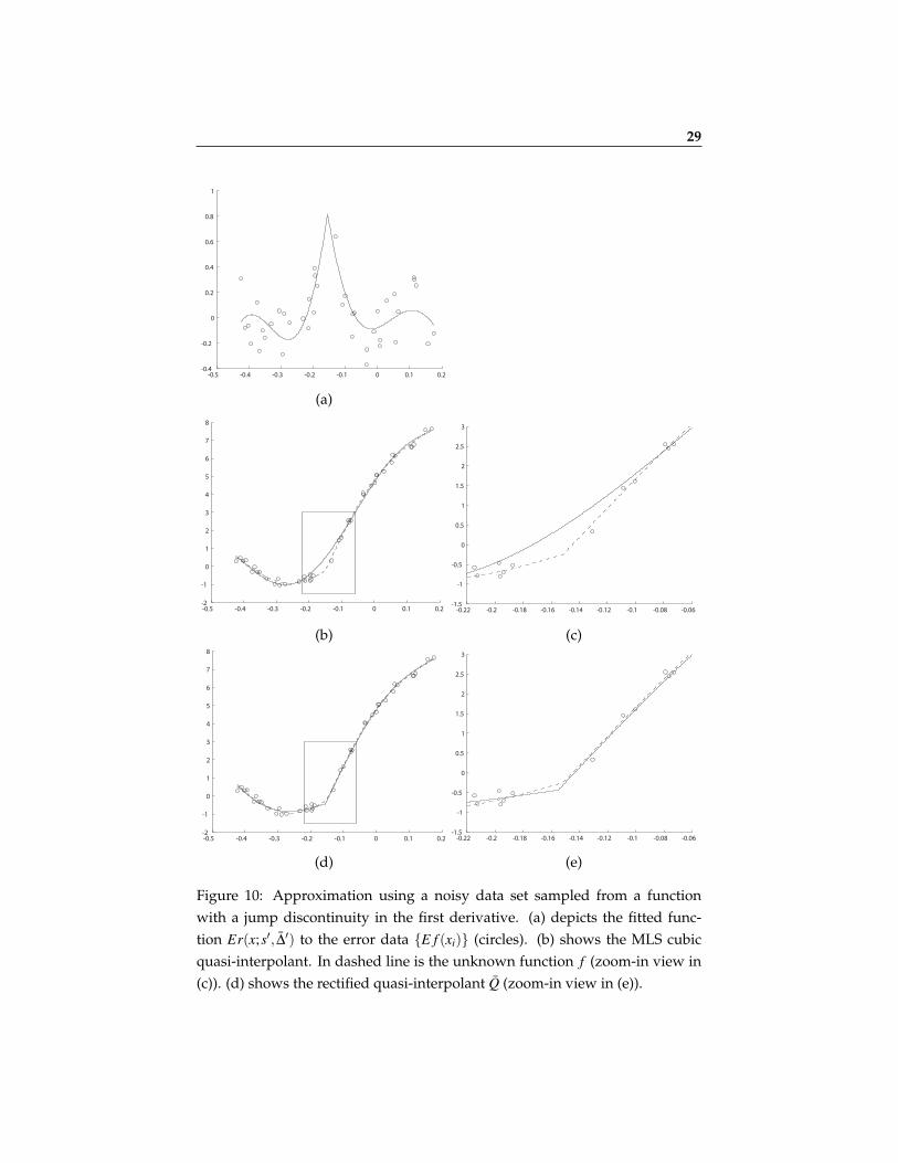
Figure 3 demonstrates an approximation of a smooth function with a jump inthe second derivative using only a few data points (8 or 17). Here we usedthe Moving Least Squares on irregular nodes. (c) and (e) demonstrate the ro-bustness and accuracy of the optimization process. Following Remark 2.1, theminimization of the functional in (9) reduces to a non-linear minimization in asingle variable s′. By Appendix A, in each interval the functional boils downto a rational function of s′ with no poles.Figure 4 demonstrates an approximation of a function with a jump in the firstderivative. In this example we used quadratic quasi-interpolating splines onregular nodes.In Figures 5-7 we compare the approximation order of the singularity location,that is |s∗− s|, with the subcell resolution method [1]. In these comparisons wehave used the same number of nodes in both methods to locate the singularitywithin a given cell. In these examples we consider singularity models differentfrom the one we treated in Section 3.1. As shown in Figure 7, the polynomialintersection method is not very efficient in the case of a smooth function witha jump in the second derivative.In Figure 8 we present a two-dimensional example, where a 2D-function’s sin-gularity curve also possesses a point singularity. In this example we have usedthe univariate detection algorithm twice: First we approximated the singular-ity along the x-axis for each row of data points, and then used the resulting ap-proximations as univariate functional data along the y-axis to locate its pointsingularity. The figure depicts the resulting approximated curve singularityalong with the true singularity curve.We experimented with the method applying it to a smooth function. The re-sults are presented in Figure 9. Among other things, in this example the mag-nitude ∆∗1 tend to zero at the rate of O(h5). This experiment shows that “ghostsingularities” may be identified by checking the convergence of ∆∗1 to zero. Onthe other hand, it shows that such singularities do not affect the approximationto the function.Finally, we have experimented with data samples contaminated with noise(Figure 10). Generally, the tradeoff between the noise size ε and the mesh sizeh can be explained as follows: For a function with a jump singularity at its k-th derivative we expect, using a quasi-interpolation method Q of degree m, anO(hm+1) approximation order away from the singularity and the error becomesO(hk) in a vicinity of the singularity. Hence, as long as the errors near the sin-gularity are larger than the noise level ε , the detection method still works. An

20

example is presented in Figure 10.

In this paper we have presented a new method for alleviating quasi-interpolationtechniques to approximate piecewise-smooth data, retaining their approxima-tion power. This is done by a general method of fitting the error in approximat-ing the singularity to the error in the approximation. The method is particu-larly efficient for locally supported quasi-interpolation operators, and is shownto be very effective for uniform and non-uniform distributions of data points.We have demonstrated the generality of the method by applying it to severalsingularity models. In the case where not all the function’s derivatives havejump discontinuity, we observed a higher order of approximation of the lo-cation and size of the jumps. In particular we have proved an O(h2(m+b)−1)approximation order to the singularity location and magnitude for functionswith a jump in their first derivative. In that case we have also provided aclosed-form solution to the minimization problem.We believe that the general methodology of locally fitting a singularity modelto the errors in a non-interpolatory approximation procedure bears further pos-sible applications in higher dimensions.

Appendix A

Theorem A.1 Fixing s in (9) results in a non-singular linear system for ∆̄ =(∆1, ...,∆m).In particular the functional in (9) is a rational function of s in each interval [xk,xk+1],with no poles in the interval.

Proof. It is enough to show that the vectors H1(X ;s),H2(X ;s), ...,Hm(X ;s), where(H j(x;s))i = H j(xi;s) and H is defined in (7), are linearly independent.Note that

H j(X ;s) = T (X− s) j+ = R∆

m+1(X− s) j+,

where T is defined in (32). Let B ∈ N+ such that Q reproduce polynomials ofmaximal degree m+B on the nodes X . Using the summation by parts formula(33), m+B− j and m+B− j +1 times we get

〈H j,X `〉 = 0, `≤ m+B− j−1 (37)

〈H j,Xm+B− j〉 6= 0,

21

-0.25 -0.2 -0.15 -0.1 -0.05 0 0.05 0.1 0.15 0.2 0.25-0.2

-0.15

-0.1

-0.05

0

0.05

0.1

0.15

0.2

0.25

0.3

-0.25 -0.2 -0.15 -0.1 -0.05 0 0.05 0.1 0.15 0.2 0.25-0.2

-0.15

-0.1

-0.05

0

0.05

0.1

0.15

0.2

0.25

0.3

(a) (b)

-0.5 -0.4 -0.3 -0.2 -0.1 0 0.1 0.2 0.3

0

0.5

1

1.5

2

2.5

3

-0.5 -0.4 -0.3 -0.2 -0.1 0 0.1 0.2 0.3

0

0.5

1

1.5

2

2.5

3

(c) (d)

Figure 2: Approximation of a function with an unknown singularity of the typec|x− s|α+, where the magnitude c, location s and the exponent α are unknown.(a,c) show the approximations using cubic MLS. A dashed line represents theunknown function f and the solid line denotes the MLS approximant. (b,d)show the MLS augmented with the fitted singular function. In (a-b) the datawere taken from a smooth function with singularity at s = π/100 and exponentα =√

3 and in (c-d) the unknown exponent is α = 1/√

3.

22

-0.3 -0.2 -0.1 0 0.1 0.2

-0.15

-0.14

-0.13

-0.12

-0.11

-0.1

-0.09

-0.08

-0.07

-0.06

-0.05

-0.3 -0.2 -0.1 0 0.1 0.2

-0.15

-0.14

-0.13

-0.12

-0.11

-0.1

-0.09

-0.08

-0.07

-0.06

-0.05

(a) (b)

-0.25 -0.2 -0.15 -0.1 -0.05 0 0.05 0.1 0.15 0.2 0.25

-23

-22

-21

-20

-19

-18

-17

-16

-15

-14

-0.4 -0.3 -0.2 -0.1 0 0.1 0.2-3

-2

-1

0

1

2

3

4

5

6x 10

-3

(c) (d)

-0.25 -0.2 -0.15 -0.1 -0.05 0 0.05 0.1 0.15 0.2 0.25

-26

-24

-22

-20

-18

-16

-0.25 -0.2 -0.15 -0.1 -0.05 0 0.05 0.1 0.15 0.2 0.25

-1

-0.8

-0.6

-0.4

-0.2

0

0.2

0.4

0.6

0.8

1

x 10-3

(e) (f)

Figure 3: Approximation of a C1 function with a jump discontinuity in thesecond derivative, that is, f (x) = 8(x− π

100 )2+ +e−x2

+0.3sin(2x)−x−1. The datasites are irregular in this case. (c) depicts the logarithm of the error functionalvalue (9) as a function of the single parameter s′. (d) shows the fitted functionEr(x;s′, ∆̄′) to the error data {E f (x j)}, depicted with circles. In (a) the unknownfunction f is shown by a dashed line and the MLS approximation by a solidline. (b) shows the MLS augmented with the singular function (d). (e) and (f)show the logarithm of the error functional and the fitted function Er(x;s′, ∆̄′)for twice the number of data points.

23

-0.4 -0.2 0 0.2 0.4 0.6-0.035

-0.03

-0.025

-0.02

-0.015

-0.01

-0.005

0

0.005

0.01

0.015

(a)

-0.5 -0.4 -0.3 -0.2 -0.1 0 0.1 0.2 0.3 0.4 0.50.8

0.9

1

1.1

1.2

1.3

1.4

1.5

1.6

-0.5 -0.4 -0.3 -0.2 -0.1 0 0.1 0.2 0.3 0.4 0.50.8

0.9

1

1.1

1.2

1.3

1.4

1.5

1.6

(b) (c)

Figure 4: Approximation of a function with a jump discontinuity in the firstderivative, that is, f (x) = |x− π

100 |+e−x2+0.3sin(5x). (a) depicts the fitted func-

tion Er(x;s′, ∆̄′) to the error data {E f (xi)} (circles). (b) shows the approximationusing quadratic quasi-interpolating B-splines. In dashed line is the unknownfunction f . (c) shows the approximant (b) augmented with the singular func-tion (a).

24

-5 -4.5 -4 -3.5 -3 -2.5 -2-30

-25

-20

-15

-10

-5

16

12

8

16

12

8

log(h)

log

|s-s

* |

Total points number 8 12 16

Poly-intersect O(h4.1) O(h6) O(h7.7)Quasi-interp method O(h4.8) O(h8.7) O(h14)

Figure 5: Comparison with the subcell resolution method w.r.t the total num-ber of points used. The singularity model here takes into account a jump in thefirst and the second derivatives. The function used f (x) = |x− π/3|+

√2(x−

π/3)2+ + e−x2

+ 0.3sin(5x). A graph of log |s− s∗| versus logh is depicted. Thetotal number of points used is written by the relevant curve. Circle markersdenote the method presented in the paper. Asterisks markers show the poly-nomial intersection (subcell resolution) method.

25

-5 -4.5 -4 -3.5 -3 -2.5 -2-35

-30

-25

-20

-15

-10

-5

16

12

8

16

12

8

log(h)

log

|s-s

* |

Total points number 8 12 16

Poly-intersect O(h4.1) O(h6) O(h7.8)Quasi-interp method O(h4.1) O(h8) O(h11.5)

Figure 6: Comparison with subcell resolution method w.r.t the number ofpoints used. The singularity model here takes into account jumps upto (andincluding) the third derivative. The function used f (x) = |x− π/3|+

√2(x−

π/3)3+ + e−x2

+ 0.3sin(5x). A graph of log |s− s∗| versus logh is depicted. Thetotal number of points used is written by the relevant curve. Circle markersdenote the method presented in the paper. Asterisks markers show the poly-nomial intersection (subcell resolution) method.

26

-5 -4.5 -4 -3.5 -3 -2.5

-25

-20

-15

-10

-5

1612

8

16

12

8

log(h)

log

|s-s

* |

Total points number 8 12 16

Poly-intersect O(h1.7) O(h3) O(h3.9)Quasi-interp method O(h2.7) O(h6.9) O(h10.8)

Figure 7: Comparison with subcell resolution method w.r.t the number ofpoints used. The singularity model here takes into account a continuous firstderivative and a jump in the second and third derivative. The function usedis f (x) =

√2(x− π/3)2

+ + e−x2+ 0.3sin(5x). A graph of log |s− s∗| versus logh

is depicted. The total number of points used is written by the relevant curve.Circle markers denote the method presented in the paper. Asterisks markersshow the polynomial intersection (subcell resolution) method.

27

(a)

-1 -0.5 0 0.5 1

-1

-0.8

-0.6

-0.4

-0.2

0

0.2

0.4

0.6

0.8

1

X

Y

-0.3 -0.2 -0.1 0 0.1 0.2 0.3

0

0.1

0.2

0.3

0.4

0.5

X

Y

(b) (c)

Figure 8: 2D example. The dashed curves in (b) and (c) denote the true sin-gularity curve, and the continuous curves are the approximated singularitycurve using a two-step procedure. The circles denote the x−singularity de-tection phase results. The function used in this case is f (x,y) = e−y2−0.5x4 −0.4 +

∣∣x+ π

100 −0.1sin(2.5y)+0.4(y− π

20 )+∣∣. Numerical evaluation of the singu-

larity location along the curve, s = π

20 , yields the approximation order |s∗− π

20 |=O(h5).

28

-0.4 -0.3 -0.2 -0.1 0 0.1 0.2 0.3 0.4 0.5 0.6

0

0.2

0.4

0.6

0.8

1

1.2

1.4

1.6

1.8

-0.4 -0.3 -0.2 -0.1 0 0.1 0.2 0.3 0.4 0.5

-0.035

-0.03

-0.025

-0.02

-0.015

-0.01

-0.005

0

0.005

0.01

0.015

(a) (b)

-0.4 -0.3 -0.2 -0.1 0 0.1 0.2 0.3 0.4 0.5

-0.2

0

0.2

0.4

0.6

0.8

1

1.2

1.4

1.6

1.8

-0.5 -0.4 -0.3 -0.2 -0.1 0 0.1 0.2 0.3 0.4 0.5

-8

-6

-4

-2

0

2

4

6

8

x 10-4

(c) (d)

-0.5 -0.4 -0.3 -0.2 -0.1 0 0.1 0.2 0.3 0.4 0.5

0

0.2

0.4

0.6

0.8

1

1.2

1.4

1.6

1.8

-0.5 -0.4 -0.3 -0.2 -0.1 0 0.1 0.2 0.3 0.4 0.5

-8

-6

-4

-2

0

2

4

6

8

x 10-5

(e) (f)

h 0.16 0.08 0.04 0.02

Q max error on nodes 6.46 ·10−3 4.60 ·10−4 2.95 ·10−5 1.85 ·10−6

Q̄ max error on nodes 6.27 ·10−3 4.49 ·10−4 2.95 ·10−5 1.84 ·10−6

Q max error 1.09 ·10−2 8.55 ·10−4 8.37 ·10−5 9.36 ·10−6

Q̄ max error 3.72 ·10−2 9.61 ·10−4 8.37 ·10−5 9.26 ·10−6

|∆∗1| 1.54 0.059 0.002 6.13 ·10−5

Figure 9: The results of applying the method (using quadratic quasi-interpolating B-splines) to data sampled from smooth function f (x) = e−x2

+sin(5x). The left column depicts the Q̄ approximant in a solid line and the func-tion f in a dashed line. In the right column the error of Q̄ is a solid line and theerror of Q is a dashed line. In (a-b) h = 0.16, (c-d) h = 0.08, (e-f) h = 0.04. Thetable at the bottom summarizes the results. Note that the decreasing rate of ∆∗1is O(h5) in this case.

29

-0.5 -0.4 -0.3 -0.2 -0.1 0 0.1 0.2-0.4

-0.2

0

0.2

0.4

0.6

0.8

1

(a)

-0.5 -0.4 -0.3 -0.2 -0.1 0 0.1 0.2-2

-1

0

1

2

3

4

5

6

7

8

-0.22 -0.2 -0.18 -0.16 -0.14 -0.12 -0.1 -0.08 -0.06-1.5

-1

-0.5

0

0.5

1

1.5

2

2.5

3

(b) (c)

-0.5 -0.4 -0.3 -0.2 -0.1 0 0.1 0.2-2

-1

0

1

2

3

4

5

6

7

8

-0.22 -0.2 -0.18 -0.16 -0.14 -0.12 -0.1 -0.08 -0.06-1.5

-1

-0.5

0

0.5

1

1.5

2

2.5

3

(d) (e)

Figure 10: Approximation using a noisy data set sampled from a functionwith a jump discontinuity in the first derivative. (a) depicts the fitted func-tion Er(x;s′, ∆̄′) to the error data {E f (xi)} (circles). (b) shows the MLS cubicquasi-interpolant. In dashed line is the unknown function f (zoom-in view in(c)). (d) shows the rectified quasi-interpolant Q̄ (zoom-in view in (e)).

References 30

respectively. And since the vectors XB, ...,Xm+B−1 are linearly independent thelemma follows. �

As a simple consequence of this theorem we prove a global minimizer s∗ ofthe functional in (9) exists:

Corollary A.1 There exists a global minimizer s∗ ∈ [a,b] to the functional in (9).

Proof. We show a minimizer to the functional where ∆̄′ is taken as a functionof s′, that is ∆̄′ = ∆̄′(s′). By Theorem A.1 we have that the functional in (9)is a continuous function of s′ defined on a closed interval and therefore fromstandard argumentation has a global minima inside this interval.�

References

[1] Francesc Arandiga, Albert Cohen, Rosa Donat, and Nira Dyn. Interpola-tion and approximation of piecewise smooth functions. SIAM J. Numer.Anal., 43(1):41–57, 2005.

[2] Rick Archibald, Anne Gelb, and Jungho Yoon. Polynomial fitting for edgedetection in irregularly sampled signals and images. SIAM J. Numer. Anal.,43(1):259–279, 2005.

[3] Rick Archibald, Anne Gelb, and Jungho Yoon. Determining the loca-tions and discontinuities in the derivatives of functions. Applied NumericalMathematics, to appear, 2007.

[4] Kendall Atkinson. An Introduction to Numerical Analysis. Wiley, 1989.

[5] Samuel Daniel Conte and Carl W. De Boor. Elementary Numerical Analysis:An Algorithmic Approach. McGraw-Hill Higher Education, 1980.

[6] C. de Boor. Quasi-interpolants and approximation power of multivariatesplines, 1990.

[7] A. Gelb. Reconstruction of piecewise smooth functions from non-uniformgrid point data. Journal of Scientific Computing, 30(3):409–440, 2007.

[8] David Gottlieb and Chi-Wang Shu. On the gibbs phenomenon and itsresolution. SIAM Rev., 39(4):644–668, 1997.

References 31

[9] Ami Harten. Eno schemes with subcell resolution. J. Comput. Phys.,83(1):148–184, 1989.

[10] E. Isaacson and H. B. Keller. Analysis of Numerical Methods. Dover, NewYork, 1993.

[11] Eitan Tadmor. Filters, mollifiers and the computation of the gibbs phe-nomenon. Acta Numerica, 16:305–378, 2007.

[12] H. Wendland. Local polynomial reproduction and moving least squaresapproximation, 2000.