approximate and exact algorithms for constrained (un) weighted two-dimensional two-staged cutting...

Journal of Combinatorial Optimization, 5, 465–494, 2001c© 2001 Kluwer Academic Publishers. Manufactured in The Netherlands.

Approximate and Exact Algorithms for Constrained(Un) Weighted Two-dimensional Two-staged CuttingStock Problems

MHAND HIFI [email protected], Maison des Sciences Economiques, Universite Paris 1 Pantheon-Sorbonne 106-112, boulevard del’Hopital, 75647 Paris cedex 13, France; PRiSM-CNRS URA 1525, Universite de Versailles-Saint Quentin enYvelines, 45 avenue des Etats-Unis, 78035 Versailles cedex, France

CATHERINE ROUCAIROL [email protected] URA 1525, Universite de Versailles-Saint Quentin en Yvelines, 45 avenue des Etats-Unis, 78035Versailles cedex, France

Abstract. In this paper we propose two algorithms for solving both unweighted and weighted constrainedtwo-dimensional two-staged cutting stock problems. The problem is called two-staged cutting problem be-cause each produced (sub)optimal cutting pattern is realized by using two cut-phases. In the first cut-phase,the current stock rectangle is slit down its width (resp. length) into a set of vertical (resp. horizontal) stripsand, in the second cut-phase, each of these strips is taken individually and chopped across its length (resp.width).

First, we develop an approximate algorithm for the problem. The original problem is reduced to a series of singlebounded knapsack problems and solved by applying a dynamic programming procedure. Second, we propose anexact algorithm tailored especially for the constrained two-staged cutting problem. The algorithm starts with aninitial (feasible) lower bound computed by applying the proposed approximate algorithm. Then, by exploitingdynamic programming properties, we obtain good lower and upper bounds which lead to significant branchingcuts. Extensive computational testing on problem instances from the literature shows the effectiveness of theproposed approximate and exact approaches.

Keywords: combinatorial optimization, cutting problems, dynamic programming, single knapsack problem,optimality

1. Introduction

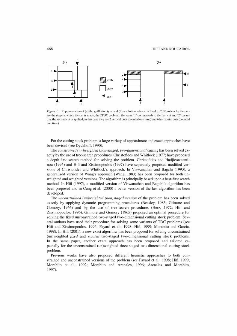
We study in this paper the problem of cutting a stock rectangle S of dimensions L×W , into nsmall rectangles (called pieces) of values (weights) ci and dimensions li ×wi , i = 1, . . . , n.Each piece i, i = 1, . . . , n, is bounded by an upper value bi , i.e., the number of occurrencesof the i-th piece in a cutting pattern (feasible solution) does not violate the value bi . Weassume that li , wi , i = 1, . . . , n, L and W are nonnegative integers and we consider thatall pieces have fixed orientation, i.e., a piece of length l and width w is different from apiece of length w and width l (when l �= w). Furthermore, all applied cuts are of guillotinetype, i.e., a horizontal or a vertical cut on a (sub)rectangle being a cut from one edge ofthe (sub)rectangle to the opposite edge which is parallel to the two remaining edges (seefigure 1(a)).

466 HIFI AND ROUCAIROL

Figure 1. Representation of (a) the guillotine type and (b) a solution when k is fixed to 2; Numbers by the cutsare the stage at which the cut is made; the 2TDC problem: the value ‘1’ corresponds to the first cut and ‘2’ meansthat the second cut is applied; in this case they are 2 vertical cuts (counted one time) and 6 horizontal cuts (countedone time).

For the cutting stock problem, a large variety of approximate and exact approaches havebeen devised (see Dyckhoff, 1990).

The constrained (un)weighted (non-staged) two-dimensional cutting has been solved ex-actly by the use of tree-search procedures. Christofides and Whitlock (1977) have proposeda depth-first search method for solving the problem. Christofides and Hadjiconstanti-nou (1995) and Hifi and Zissimopoulos (1997) have separately proposed modified ver-sions of Christofides and Whitlock’s approach. In Viswanathan and Bagchi (1993), ageneralized version of Wang’s approach (Wang, 1983) has been proposed for both un-weighted and weighted versions. The algorithm is principally based upon a best-first searchmethod. In Hifi (1997), a modified version of Viswanathan and Bagchi’s algorithm hasbeen proposed and in Cung et al. (2000) a better version of the last algorithm has beendeveloped.

The unconstrained (un)weighted (non)staged version of the problem has been solvedexactly by applying dynamic programming procedures (Beasley, 1985; Gilmore andGomory, 1966) and by the use of tree-search procedures (Herz, 1972; Hifi andZissimopoulos, 1996). Gilmore and Gomory (1965) proposed an optimal procedure forsolving the fixed unconstrained two-staged two-dimensional cutting stock problem. Sev-eral authors have used their procedure for solving some variants of TDC problems (seeHifi and Zissimopoulos, 1996; Fayard et al., 1998; Hifi, 1999; Morabito and Garcia,1998). In Hifi (2001), a new exact algorithw has been proposed for solving unconstrained(un)weighted fixed and rotated two-staged two-dimensional cutting stock problems.In the same paper, another exact approach has been proposed and tailored es-pecially for the unconstrained (un)weighted three-staged two-dimensional cutting stockproblem.

Previous works have also proposed different heuristic approaches to both con-strained and unconstrained versions of the problem (see Fayard et al., 1998; Hifi, 1999;Morabito et al., 1992; Morabito and Arenales, 1996; Arenales and Morabito,1997).

APPROXIMATE AND EXACT ALGORITHMS 467

2. The two-dimensional (staged) cutting problem

We say that the n-dimensional vector (x1, . . . , xn) of integer and nonnegative numberscorresponds to a cutting pattern, if it is possible to produce xi pieces of type i, i = 1, . . . , n,in the stock rectangle S without overlapping and without violating the upper values bi .The constrained Two-Dimensional Cutting problem (shortly constrained TDC) consists ofdetermining the cutting pattern (using guillotine cuts) with the maximum value, i.e.,

constrained TDC =

maxn∑

i=1

ci xi

subject to (x1, . . . , xn) ≤ (b1, . . . , bn)

corresponds to a cutting pattern

(1)

In constrained TDC problem one has, in general, to satisfy a certain demand of pieces,i.e., the upper values bi , i = 1, . . . , n. The problem is called unconstrained if these demandvalues are not imposed. In this case, the cutting pattern of Eq. (1) can be represented by(x1, . . . , xn) ≤ (b′

1, . . . , b′n), where b′

i = � Lli� W

wi, for i = 1, . . . , n, which represents a

natural upper bound-value for each considered piece.We distinguish two versions of the constrained TDC problem: the unweighted version in

which the weight ci of the i-th piece is exactly its area, i.e., ci = liwi , and the weightedversion in which the weight of each piece is independent of its area, i.e., there exists a piece� for which c� �= l�w�, 1 ≤ � ≤ n.

Another variant of the TDC problem is to consider a constraint on the total number ofcuts, i.e., the sum of some parallel vertical and/or horizontal cuts (using guillotine cuts) doesnot exceed a certain constant k < ∞. In this case the problem is called the staged TDCproblem or k-staged TDC problem (shortly kTDC). Figure 1(b) shows a 2TDC solutionwhich is produced by applying the following phases:

Phase 1. the stock rectangle is slit down its width into a set of vertical strips;Phase 2. each of these vertical strips is taken individually and chopped across its length.

For simplicity, for the constrained (un)weighted kTDC problem, we use the same nota-tions as introduced in Hifi (2001):

– C kTDC: corresponds to the Constrained (un)weighted kTDC problem. This notationis used if we consider (a) unweighted and weighted versions, and (b) the fixed and therotated cases (in the rotated case, we consider that each piece can be turned of 90◦).

– FC kTDC: corresponds to the Fixed Constrained (un)weighted kTDC problem. Thisnotation is used when we refer to unweighted and weighted versions of the problem;

– FCU kTDC: represents the Fixed Constrained Unweighted kTDC problem;– FCW kTDC: corresponds to the Fixed Constrained Weighted kTDC problem.

Definition 1. Let (L , β) (resp. (α, W )) be the dimensions of a strip entering in the stockrectangle S. Then,


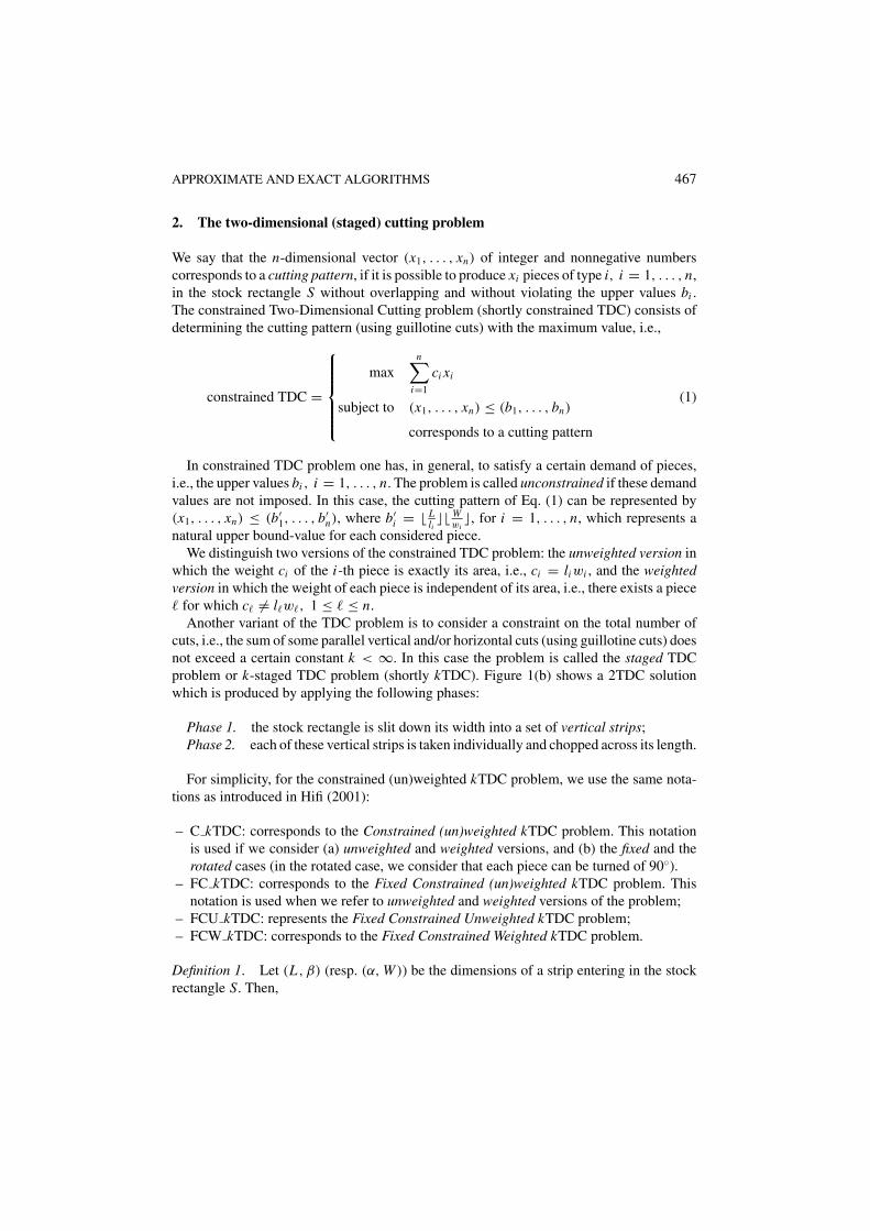
Figure 2. Representation of (a) a stock rectangle with three pieces to cut and (b) three different strips; (b.1) and(b.2) are two strips without trimming and (b.3) represents a strip with trimming.

• (L , β) (resp. (α, W )) represents a uniform horizontal (resp. vertical) strip if it is composedof different pieces having the same width (resp. length).

• (L , β) (resp. (α, W )) represents a general horizontal (resp. vertical) strip if it contains atleast two pieces with different widths (resp. lengths) which participate to the compositionof the strip.

Example 1. Consider the instance problem of figure 2(a). It is composed of a stock rect-angle of dimensions (L , W ) = (11, 7) and three pieces p1, p2 and p3 respectively ofdimensions (6, 3), (4, 3) and (1, 2) respectively.

Figure 2(b.1) shows a uniform horizontal strip with dimensions (11, 2). The consideredstrip is composed of the same piece with width β = 2 and with value equal to 22. We saythat the obtained strip is without trimming, i.e., vertical cuts are sufficient to produce allparticipated pieces (for the considered strip).

Also, figure 2(b.2) shows another uniform horizontal strip with dimensions (11, 3) andwith value equal to 30. This strip contains two pieces of type p1 and p2 respectively, havingthe same width β = 3. It is also obtained without trimming.

Now, consider figure 2(b.3). The obtained strip (of dimensions (L , β) = (11, 3) and withvalue 32) represents a general horizontal strip, because some pieces have different widths(in this example, the width of p1 is equal to 3 and the width of p3 is equal to 2). Wesay that the strip is obtained with trimming, i.e., vertical cuts are not sufficient to produceall participated pieces and so, supplementary horizontal cuts are necessary to extract somepieces (in figure 2(b.3), the piece p3 is obtained by applying a supplementary horizontal cut).

According to Definition 1 and the strips illustrated by figures 2(b), we can distinguish twocases of the staged cutting problem. The first one is considered when trimming is permitted(called the nonexact case in Gilmore and Gomory (1965), Hifi (2001) and Morabito andGarcia (1998)) and the second one represents the exact case in which trimming is notpermitted.

In this paper we treat both FCU 2TDC and FCW 2TDC problems by considering theexact (without trimming) and the nonexact (trimming is permitted) cases.

The paper is organized as follows. First (Section 3), we describe an extended version ofGilmore and Gomory’s procedure (1965) applied especially for providing an approximate


solution to both FCU 2TDC and FCW 2TDC problems. Both exact and non-exact versionsof the problem are considered. In Section 3.3, we propose an improved version of theapproximate algorithm. Third (Section 4), we present an approximate algorithm for thenon-exact case, i.e., trimming is permitted. In Section 5, we develop an exact algorithmfor solving unweighted and weighted FC 2TDC problems and by considering the non-trimming case. Section 6 presents an exact algorithm when trimming is permitted. Theobtained algorithm is an adaptation of the algorithm proposed in Section 5. Finally, theperformance of the proposed algorithms are presented in Section 7. A set of large sizeproblem instances is considered and benchmark results are given. To our knowledge, noother exact solution procedure for the FC 2TDC problem exists in the literature.

3. An approximate algorithm for FC 2TDC: Without trimming

In this section, we describe the procedure applied for solving both FCU 2TDC andFCW 2TDC problems. The procedure was originally applied by Gilmore and Gomory(1965) for the fixed unconstrained 2TDC problem and improved later in Hifi (2001). Herewe apply an extended version of the procedure by imposing the demand values on eachconsidered piece. Moreover, our procedure can be applied for the two cases of the problem:(i) without trimming and (ii) with trimming.

The procedure is composed of two phases. The first phase is composed of two stages:the first stage is applied in order to construct a set of different horizontal strips and, thesecond one is applied for combining some horizontal strips for producing an approximatehorizontal cutting pattern. The second phase of the procedure is also composed of twostages: first, we try to construct a set of vertical strips and we combine some of them forobtaining an approximate vertical cutting pattern.

3.1. The first phase: A horizontal cutting pattern

The first stage. The problem of generating some horizontal bounded strips can be summa-rized as follows: without loss of generality, assume that the pieces are ordered in nondecreas-ing order such that w1 ≤ w2 ≤ · · · ≤ wn . Suppose that r denotes the number of differentwidths of the considered pieces (i.e. we have the following order w1 < w2 < · · · < wr ,where ∀ j ∈ {1, . . . , r}, w j ∈ {w1, . . . , wn}), and (L , w j ) is a strip with width w j . Wedefine the single Bounded Knapsack problems (BKhor

L ,w j), for j = 1, . . . , r , as follows:

(BKhor

L ,w j

)

f horw j

(L) = max∑

i∈SL ,w j

ci xi

subject to∑

i∈SL ,w j

li xi ≤ L

xi ≤ bi , xi ∈ IN , i ∈ SL ,w j

where SL ,w j is the set of pieces entering in the strip (L , w j ) such that ∀k ∈ SL ,w j , wk = w j

(i.e., all pieces have the same width), xi denotes the number of times the piece i appears in


the j-th horizontal strip without exceeding the value bi , ci is the weight associated to thepiece i ∈ SL ,w j and f hor

w j(L) is the solution value of the j-th strip, j = 1, . . . , r .

Remark 1. It consists in solving a series of small independent single bounded knapsackproblems BKhor

L ,w1, BKhor

L ,w2, . . . , BKhor

L ,wr, respectively. These problems are independent and

their resolution is equivalent to solve only a largest single bounded knapsack with n pieces.

The second stage. The aim of this step is to select the best of these horizontal strips forobtaining an approximate cutting pattern to the FC 2TDC problem. We do it by solvinganother single Bounded Knapsack Problem, given as follows:

(BKPhor

(L ,W )

)

ghorL (W ) = max

r∑j=1

f horw j

(L)y j

subject tor∑

j=1

w j y j ≤ W

y j ≤ a j , y j ∈ IN

where y j , j = 1, . . . , r , is the number of occurrences of the j-th horizontal strip in thestock rectangle S, bounded by its upper bound-value a j , f hor

w j(L) is the solution value of the

j-th strip and ghorL (W ) is the solution value of the cutting pattern, for the rectangle (L , W ),

composed of some horizontal strips. It is clear that each horizontal strip j, j = 1, . . . , r ,can be appeared at least one time and at most � W

w j times in the stock rectangle.

Let δi j be the number of times the i-th piece appears in the j-th strip. So, we can easilyremark that a possible way for computing each a j is the following:

a j = min

{⌊W

w j

⌋, min

1≤i≤n

{⌊bi

δi j

⌋ ∣∣∣∣ δi j > 0

}}, j = 1, . . . , r. (2)

3.2. The second phase: A vertical cutting pattern

The first stage. By applying the same process as in Section 3.1 (first stage), we can generatethe set of the vertical strips such that:

• we consider that pieces are ordered in nondecreasing order such that l1 ≤ l2 ≤ · · · ≤ ln;• we reverse the role of widths and lengths in the previous single bounded knapsack prob-

lems BKhorL ,w j

, i.e., w j by l j , li by wi , L by W, f horw j

(L) by f verl j

(W ) and r by s (where s

denotes the number of distinct lengths such that l1 < l2 < · · · < ls).

We denote the resulting single bounded knapsack problems by BKverl j ,W

, for j = 1, . . . , s.For more clarity, we present below each problem corresponding to the j-th length, where


j = 1, . . . , s.

(BKver

l j ,W

)

f verl j

(W ) = max∑

i∈Sl j ,W

ci xi

subject to∑

i∈Sl j ,W

wi xi ≤ W

xi ≤ bi , xi ∈ IN , i ∈ Sl j ,W

where Sl j ,W is the set of pieces entering in the vertical strip (l j , W ) such that ∀k ∈ Sl j ,W , lk =l j (i.e., all pieces have the same length), xi denotes the number of times the piece i appearsin the j-th vertical strip without exceeding the value bi , ci is the weight associated to thepiece i ∈ Sl j ,W and f ver

l j(W ) is the solution value of the j-th vertical strip, j = 1, . . . , s.

So, by solving these independent problems, we obtain the set of vertical strips.

The second stage. In this section, we also apply the same process as in Section 3.1 (secondstage). Indeed, we construct an approximate vertical cutting pattern by solving the followingsingle bounded knapsack:

(BKPver

(L ,W )

)

gverW (L) = max

s∑j=1

f verl j

(W )y j

subject tos∑

j=1

l j y j ≤ L

y j ≤ ai , y j ∈ IN

where (BKPver(L ,W )) is obtained by replacing in the above problem (BKPhor

(L ,W )), w j by l j , Wby L , ghor

L (W ) by gverW (L), r by s (where s is the number of distinct lengths) and

a j = min

{⌊L

l j

⌋, min

1≤i≤n

{⌊bi

δi j

⌋ ∣∣∣∣ δi j > 0

}}, j = 1, . . . , s, (3)

where δi j is the number of times that piece i appears in the j-th vertical strip.

Remark 2. If we consider that the first-stage cut is unspecified (i.e., the first cut is madehorizontally or vertically), then the approximate solution to the FC 2TDC problem is theone that realizes the best solution value between horizontal and vertical feasible two-stagedpatterns, i.e., the pattern realizing the value max{ghor

L (W ), gverW (L)}.

3.3. Enhancing the approximate algorithm

In this part, we present a simple improvement to the previous approximate algorithm. Theproblems (BKhor

L ,w j) are used for producing a set of r optimal horizontal strips and, combined


later by applying one problem (BKPhor(L ,W )). The same process is applied for creating the s

optimal vertical strips and, combined later by solving the problem (BKPver(L ,W )).

The improvement consists in generating other horizontal (resp. vertical) substrips inorder to combine them by applying the same problem (BKPhor

(L ,W )) (resp. (BKPver(L ,W ))). All

horizontal substrips are constructed by using the following procedure:

1. Let r be the number of the optimal horizontal strips, obtained by solving the largestproblem (BKhor

L ,wr), where wr ∈ {w1, . . . , wn}.

2. let a j , j = 1, . . . , r , be the maximum number that the j-th horizontal strip can beappeared in the stock rectangle (L , W ) (see Eq. (2)).For each strip j, j = 1, . . . , r , compute b′

i as follows:

b′i = bi − a j ∗ δi j

where δi j denotes the number of times that piece i appears in the j-th strip.3. If there exists a component b′

i , such that b′i > 0, then solve the problem (BKhor

L ,wr ′ ), wherer ′ is the number of the new substrips and wr ′ is equal to max1≤i≤n{wi | b′

i > 0}.4. Let r = r + r ′ be the number of the available (sub)strips. Then, solve (BKPhor

(L ,W )) byconsidering the new number r of (sub)strips and by setting a j , j = r + 1, . . . , r + r ′,equal to

min

{⌊W

w j

⌋, min

1≤i≤n

{⌊b′

i

δi j

⌋ ∣∣∣∣ δi j > 0

}}.

Of course, we apply the same procedure for the vertical substrips, by replacing r by s, r ′

by s ′ and, by solving (BKverls′ ,W

) and (BKPver(L ,W )). Limited computational results showed that

such an improvement, i.e., applying the above procedure one time, produces a satisfactorysolution to the problem.

4. An approximate algorithm for FC 2TDC: Trimming is permitted

In this section, we present an approximate algorithm for the non-exact case (trimmingis permitted). Clearly, the approximate algorithm used for the exact case of the problem(without trimming) is also an approximate algorithm for the non-exact case. So, we applythe improved version of the algorithm (Section 3.3) for computing the first approximatesolution to the non-exact case of the problem.

In Hifi (1997), another approximate algorithm has been developed for starting the exactapproach used for solving the non-staged constrained cutting problem. This approximatealgorithm is composed of two steps:

1. constructing a set of general horizontal (resp. vertical) strips (see Definition 1);2. combining some of these general horizontal (resp. vertical) strips for obtaining an ap-

proximate solution to the non-staged constrained TDC problem. The solution is obtainedthrough a set packing problem.


This solution can also be considered as an approximate solution to the FC 2TDC problemwhen trimming is permitted. In what follows, we try to summarize the approach and formore details, the reader can be referred to Hifi (1997).

The first stage. The first stage represents the first phase of Section 3.1 (resp. Section 3.2)using a slight modification. In order to construct the set of horizontal (resp. vertical) strips,we consider the same problem BKhor

L ,w j(resp. BKver

l j ,W) and we reorder all pieces of each

set SL ,w j , j = 1, . . . , r (resp. Sl j ,W , j = 1, . . . , s) which represents the set of rectangularpieces entering in the strip (L , w j ) (resp. (l j , W )). For each index j of SL ,w j (resp. Sl j ,W ),we have (li , wi ) ≤ (L , w j ) (resp (li , wi ) ≤ (l j , W )).

In this case, by applying a dynamic programming procedure, we only solve the largestproblem BKhor

L ,wr(resp. BKver

ls ,W), where wr = max1≤i≤n{wi } (resp. ls = max1≤i≤n{li }).

The second stage. The second stage consists in selecting the best of these general optimalhorizontal/vertical strips for constructing an approximate horizontal/vertical cutting pat-tern. This can be realized, by solving the following set (strip) packing problems (Phor

(L ,W ))

and (Pver(L ,W )), respectively:

(Phor

(L ,W )

)

ghorL (W ) = max

r∑j=1

f horw j

(L)y j

subject tor∑

j=1

w j y j ≤ W

r∑j=1

δi j y j ≤ bi

i = 1, . . . , n, y j ∈ IN

(Pver

(L ,W )

)

gverW (L) = max

s∑j=1

f verl j

(W )z j

subject tos∑

j=1

l j z j ≤ L

s∑j=1

δi j z j ≤ bi

i = 1, . . . , n, z j ∈ IN

where y j , j = 1, . . . , r (resp. z j , j = 1, . . . , s) is the number of occurrences of the j-thstrip in the stock rectangle S, δi j is the number of occurrences of the i-th piece in thej-th strip and ghor

L (W ) (resp. gverW (L)) is the solution value of the horizontal (resp. vertical)

cutting pattern.Consequently, when we deal with the initial rectangle (L , W ), we need to solve two

set packing problems. Of course, the set packing problem is NP-complete and the methodused to approximately solve this problem will significantly influence the algorithm perfor-mance. In our computational results, on one hand, we have used a simple greedy algorithm


(for more details the reader is referred to Hifi, 1997) and the approximate solution of Sec-tion 3.3, and we take the better solution as the solution to the non-exact case.

5. An exact algorithm for the FC 2TDC: Without trimming

Branch-and-Bound (B&B) is a well-known technique for solving combinatorial searchproblems. Its basic scheme is to reduce the problem search space by dynamically pruningunsearched areas which cannot yield better results than already found. The B&B methodsearches a finite space T , implicitly given as a set, in order to find one state t∗ ∈ T which isoptimal for a given objective function f . Generally, this approach proceeds by developing atree in which each node represents a part of the state space T . The root node represents theentire state space T . Nodes are branched into new nodes which means that a given part T ′

of the state space is further split into a number of subsets, the union of which is equal to T ′.Hence, the optimal solution over T ′ is equal to the optimal solution over one of the subsetsand the value of the optimal solution over T ′ is the minimum (or maximum) of the optimaover the subsets. The decomposition process is repeated until the optimal solution over thepart of the state space is reached.

The proposed approach uses a simple strategy for solving exactly the FC 2TDC problem.This strategy can be summarized as follows:

1. Starting by an initial (feasible) lower bound;2. Constructing a set of horizontal/vertical (sub)strips;3. Combining some of these (sub)strips for producing an optimal solution to the FC 2TDC

problem.

5.1. An exact algorithm for the horizontal FC 2TDC problem: Without trimming

5.1.1. Uniform horizontal substrips and the optimal horizontal solution on (L, W ). Theconstruction of each horizontal (sub)strip is obtained by combining all pieces and theircopies by horizontal builds. In what follows, we use the Wang’s construction (see Wang,1983 and initially used by Albano and Sapuppo, 1980) for obtaining the different horizontal(sub)strips and (sub)optimal solutions. Of course, the definition is also applicable when weconsider the construction of the vertical strips.

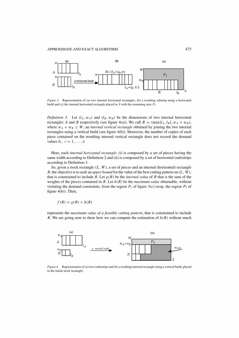
Definition 2. Let (lA, w) and (lB, w) be the dimensions of two substrips A and B (seefigure 3(a)). We call R = (lA + lB, w), where lA + lB ≤ L , an internal horizontal rectangle(substrip) obtained by joining the two patterns using a horizontal build (see figure 3(b)).Moreover, the number of copies of each piece contained on the resulting internal horizontalrectangle does not exceed the demand values bi , i = 1, . . . , n.

Also, the optimal horizontal solution (which is also an internal horizontal rectangle) tothe FC 2TDC problem is obtained by combining some horizontal substrips and/or someinternal horizontal rectangles having the strip structure. Each of these rectangles is obtainedby applying a vertical build according to the following definition.


Figure 3. Representation of (a) two internal horizontal rectangles, (b) a resulting substrip using a horizontalbuild and (c) the internal horizontal rectangle placed in S with the remaining area P1.

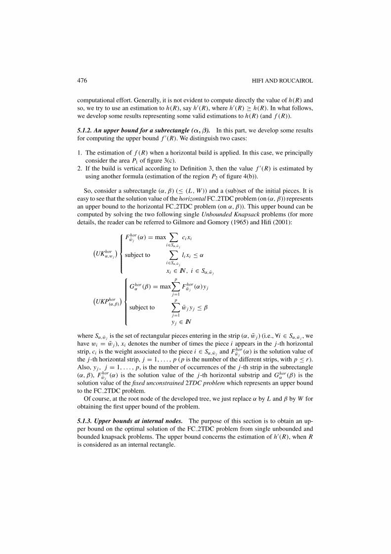
Definition 3. Let (lA, wA) and (lB, wB) be the dimensions of two internal horizontalrectangles A and B respectively (see figure 4(a)). We call R = (max{lA, lB}, wA + wB),where wA + wB ≤ W , an internal vertical rectangle obtained by joining the two internalrectangles using a vertical build (see figure 4(b)). Moreover, the number of copies of eachpiece contained on the resulting internal vertical rectangle does not exceed the demandvalues bi , i = 1, . . . , n

Here, each internal horizontal rectangle: (i) is composed by a set of pieces having thesame width according to Definition 2 and (ii) is composed by a set of horizontal (sub)stripsaccording to Definition 3.

So, given a stock rectangle (L , W ), a set of pieces and an internal (horizontal) rectangleR, the objective is to seek an upper bound for the value of the best cutting pattern on (L , W ),that is constrained to include R. Let g(R) be the internal value of R that is the sum of theweights of the pieces contained in R. Let h(R) be the maximum value obtainable, withoutviolating the demand constraints, from the region P1 of figure 3(c) (resp. the region P2 offigure 4(b)). Then,

f (R) = g(R) + h(R)

represents the maximum value of a feasible cutting pattern, that is constrained to includeR. We are going now to show how we can compute the estimation of h(R) without much

Figure 4. Representation of (a) two (sub)strips and (b) a resulting internal rectangle using a vertical build, placedin the initial stock rectangle.


computational effort. Generally, it is not evident to compute directly the value of h(R) andso, we try to use an estimation to h(R), say h′(R), where h′(R) ≥ h(R). In what follows,we develop some results representing some valid estimations to h(R) (and f (R)).

5.1.2. An upper bound for a subrectangle (α, β). In this part, we develop some resultsfor computing the upper bound f ′(R). We distinguish two cases:

1. The estimation of f (R) when a horizontal build is applied. In this case, we principallyconsider the area P1 of figure 3(c).

2. If the build is vertical according to Definition 3, then the value f ′(R) is estimated byusing another formula (estimation of the region P2 of figure 4(b)).

So, consider a subrectangle (α, β) (≤ (L , W )) and a (sub)set of the initial pieces. It iseasy to see that the solution value of the horizontal FC 2TDC problem (on (α, β)) representsan upper bound to the horizontal FC 2TDC problem (on α, β)). This upper bound can becomputed by solving the two following single Unbounded Knapsack problems (for moredetails, the reader can be referred to Gilmore and Gomory (1965) and Hifi (2001):

(UKhor

α,w j

)

Fhorw j

(α) = max∑

i∈Sα,w j

ci xi

subject to∑

i∈Sα,w j

li xi ≤ α

xi ∈ IN , i ∈ Sα,w j

(UKPhor

(α,β)

)

Ghorα (β) = max

p∑j=1

Fhorw j

(α)y j

subject top∑

j=1

w j y j ≤ β

y j ∈ IN

where Sα,w j is the set of rectangular pieces entering in the strip (α, w j ) (i.e., ∀i ∈ Sα,w j , wehave wi = w j ), xi denotes the number of times the piece i appears in the j-th horizontalstrip, ci is the weight associated to the piece i ∈ Sα,w j and Fhor

w j(α) is the solution value of

the j-th horizontal strip, j = 1, . . . , p (p is the number of the different strips, with p ≤ r ).Also, y j , j = 1, . . . , p, is the number of occurrences of the j-th strip in the subrectangle(α, β), Fhor

w j(α) is the solution value of the j-th horizontal substrip and Ghor

α (β) is thesolution value of the fixed unconstrained 2TDC problem which represents an upper boundto the FC 2TDC problem.

Of course, at the root node of the developed tree, we just replace α by L and β by W forobtaining the first upper bound of the problem.

5.1.3. Upper bounds at internal nodes. The purpose of this section is to obtain an up-per bound on the optimal solution of the FC 2TDC problem from single unbounded andbounded knapsack problems. The upper bound concerns the estimation of h′(R), when Ris considered as an internal rectangle.


The horizontal construction that we have considered for producing the set of horizontalbuilds can be viewed as a two stage method:

1. a horizontal build provides an internal horizontal rectangle R,2. an estimation of h′(R) attempts to minimize the upper bound f ′(R), when R is considered

as a (feasible) solution to the FC 2TDC problem. In this case, we can reject some(sub)strips if their upper bounds is not greater than the best current feasible solutionvalue.

The first point is realized by applying Definition 2 and the second point, which corre-sponds to the value of f ′(R), is represented by the following results.

Lemma 1. Let {(α, β1), (α, β2), . . . , (α, βm)} be a set of horizontal substrips having thesame length α. Suppose that all widths βi , i = 1, . . . , m, are given in nondecreasing orderand each substrip (α, βi ) is characterized by its solution value Fhor

βi(α). Then, only one single

knapsack problem permits to produce the upper bounds to all considered subrectangles(α,γ ), where 0 ≤ γ ≤ βm.

Proof: Consider the fictive subrectangle (α, β), where

β = max1≤i≤m

{βi }.

By applying a dynamic programming procedure to the resulting problem (UKPhorα,β), we

obtain:

1. an upper bound for the fictive rectangle (α, β), with value Ghorα (β),

2. an upper bound to each subrectangle (α, y), with value Ghorα (y) such that y ≤ β.

We recall that this is possible because dynamic programming techniques are considered.Hence, if x (=βi ) coincides with one of the widths of the set {β1, β2, . . . , βm}, then necessarywe have the solution value Ghor

α (βi )which corresponds to an upper bound to the subrectangle(α, βi ). ✷

In particular, if we consider that β1 = w1, β2 = w2, . . . , βm = wm , where m ≤ r , and byapplying a dynamic programming procedure to the problem UKPhor

L ,W , then we have neces-sary the solution value Ghor

L (y) of each subrectangle (L , y), with 0 ≤ y ≤ W .

Lemma 2. Let (L,β) be a horizontal substrip with length L and width β, where β ≤ W .Then, the resolution of the single unconstrained knapsack problem (UKhor

L ,w j) produces an

upper bound for each substrip (x, β) with values Fhorβ (x), where x ≤ L.

Proof: We use the same reasoning as for Lemma 1.By solving initially the problem UKhor

L ,w jand by applying a dynamic programming pro-

cedure, we obtain the following results:


1. we construct the strip (L , β) with value Fhorβ (L). This solution value represents an upper

bound to the strip (L , β), when we consider the FC 2TDC problem (see Section 5.1.2),2. all substrips with dimensions (x, β), where x ≤ L − 1, are available with their solution

values Fhorβ (x). This solution value is also an upper bound to each subrectangle (x, β),

where x ≤ L . ✷

In what follows, we present upper bounds representing the area P1 of figure 3(c). Thesebounds are principally based upon single knapsack problems and the time complexity forthe computation of these bounds is apparently constant.

Theorem 1. Given an internal rectangle R with dimensions (lR, wR), a valid upper boundfor f (R), when a horizontal build is applied, is

f1(R) = g(R) + GhorL (W − wR) + Fhor

wk(L − lR) (4)

where GhorL (W − wR) is the solution value of the single unconstrained knapsack

UKPhor(L ,W−wR) and Fhor

k (L − lR) is the solution value of the single unconstrained knap-

sack UKhorL−lR ,W−wk

, where k ∈ {1, . . . , r}.

Proof: Recall that f ′(R) = g(R) + h′(R) is an upper bound to the solution containingthe internal rectangle R as one of its component. The time complexity for computing g(R)

is constant, since we just use an addition.We can remark that the optimal solution, to the constrained two-staged problem, contain-

ing the internal rectangle R is necessarily composed of a strip (L , wR) and a complementarysolution which can be represented by the second part (L , W − wR) of the stock rectangle.So, by applying Lemmas 1 and 2, we can affirm that:

1. the available value GhorL (W − wR) (of the problem UKPhor

(L ,W−wR)) represents an upperbound to the subrectangle (L , W − wR).

2. the available value FhorwR

(L − lR) (of the problem UKhorL−lR ,W−wk

) represents an upperbound to the subrectangle (L , wR), since wR coincides with one of the following widthsw1, w2, . . . , wr .

Hence, the solution value

f1(R) = g(R) + GhorL (W − wR) + Fhor

wk(L − lR) ≥ f (R)

represents an upper bound to the FC 2TDC problem, containing the internal rectangle R.Clearly, the time complexity for computing f1(R) is constant, because:

1. g(R) is computed in constant time,2. h1(R) = Ghor

L (W − wR) + Fhorwk

(L − lR) is also computed in constant time. In thiscase, we just remark that the two upper bounds corresponding to the subrectangles(L , W − wR) and (L − lR, wR) are available. ✷


The above result shows that the upper bound to the FC 2TDC problem can be obtainedby considering some remaining solution values derived from single unbounded knapsackproblems. Let us now see how we can introduce the single bounded knapsack problem forgiving another and better upper bound. This bound dominate the previous one (Eq. (4)) andits computation time complexity is also constant.

Corollary 1. A valid and a better upper bound for f (R) is

f2(R) = g(R) + GhorL (W − wR) + f hor

wk(L − lR) (5)

where f horwk

(L − lR) is the solution value of the single bounded knapsack BKhorL−lR ,W−wk

andk ∈ {1, . . . , r}.

Proof: Let BKhor(L ,wR) be the single bounded knapsack for which the width wR coincides

with a width w j , where w j ∈ {w1, . . . , wr }.By applying Lemma 2 to the problem BKhor

(L ,wR), we can deduce that all optimal substrips(x, wR), where x ≤ L , are available and so, in particular the optimal substrip (L − lR, wR)is also obtained. So, the optimal solution value f hor

wk(L − lR) represents also an upper bound

for the subrectangle (substrip) (L − lR, wR) and so,

f2(R) = g(R) + GhorL (W − wR) + f hor

wk(L − lR)

is an upper bound for the solution containing the internal rectangle R.Since the solution value f hor

wk(L − lR) denotes the value of the best solution value of

the substrip (L − lR, wR), then necessary this solution value is better than the solutionvalue Fhor

wk(L − lR). This is true because the solution value of the problem UKhor

L−lR ,W−wkis

obtained by fixing the demand values bi to � Lli� W

wi, for i = 1, . . . , n. Hence,

f horwk

(L − lR) ≤ Fhorwk

(L − lR) ⇔ f2(R) ≤ f1(R) ✷

The following result is used when the vertical build is applied for combining two hori-zontal internal rectangles, i.e. two (sub)strips. In this case, the value of h′(R) concerns theestimation of the area P2 of figure 4(b).

Theorem 2. Let A and B be two internal rectangles with dimensions (lA, wA) and (lB, wB)respectively. A valid upper bound for f (R), where R is the resulting internal verticalrectangle, is

f3(R) = g(R) + GhorL (W − wR) (6)

where GhorL (W − wR) is the solution value of UKPhor

(L ,W−wR).

Proof: Let R be the internal vertical rectangle obtained by combining vertically A and Brespectively (see figure 4).


According to Definition 3, the dimensions of R are at least equal to (max{lA, lB}, wA+wB)and since R is considered as an internal vertical rectangle, then R will never combinedhorizontally with another internal rectangle. Hence,

(lR, wR) = (L , wA + wB) (7)

and

f3(R) = g(R) + g(B) + h′(R) = g(R) + GhorL (W − (wA + wB))

= g(R) + GhorL (W − wR) (8)

since R is an internal vertical rectangle and it is considered as a strip with dimensions(L , wA + wB). ✷

ALGO. The Exact (Horizontal) Algorithm for the FC 2TDC problem.

Input: an instance of the FC 2TDC problem: a set of rectangles (R1, . . . , Rn) and astock rectangle (L , W ).Output: an optimal (horizontal) solution Best with value Opthor (Best)..• Solve the following single (un)bounded knapsack problems :

• UKL ,w j , j = 1, . . . , r (by using only the largest single knapsack) and UKhor(L ,W );

• BKL ,w j , j = 1, . . . , r (by using only the largest single knapsack) and BKhor(L ,W ).

• Set Opthor(Best) = ghorL (W );

• If Opthor(Best) = GhorL (W ) then exit with the optimal solution Best with value

Opthor (Best);• Set Open = {R1, R2, . . . , Rn};• Set Closed equal to empty set and set Stop = false;RepeatTake one internal (horizontal) rectangle R from Open having the highest value f ′;If f ′(R) − Opt(Best) ≤ 0, then Stop:= trueElseBegin

1. transfer R from Open to Closed;2. construct all internal rectangles Q such that:

(a) each element q of Q is constructed by applying a horizontal build(see Definition 2) or a vertical build (see Definition 3) of R with someinternal horizontal rectangles, say R′, of Closed;

(b) the width wR′ of each R′ of Closed is equal to wR , when thehorizontal build is applied

(c) the dimensions (lq , wq ) are less than or equal to (L , W );(d) ∀q ∈ Q, dq

i ≤ bi , i = 1, . . . , n;3. for each element q of Q, do:

(a) compute g(q);(b) compute h′(q) (using equation (5) for the horizontal build and


equations (6) or (9) when the vertical build is considered)If g(q) > Opthor (Best) then set Best = q and Opthor (Best) = g(q);If g(q) + h′(q) > Opthor (Best) then set Open = Open ∪ {q};

4. If Open = {} then Stop := true;end;

Until Stop;• Exit with the optimal solution Best with value Opthor (Best).

Corollary 2. Let R be a resulting internal rectangle constructed by combining two internalrectangles A and B. If W − wR = wmin , where wmin denotes the smallest width enteringin the strip (L , W − wR), then the valid upper bound for f (R) is

f4(R) = g(R) + ghorL (W − wR) ≤ f3(R) (9)

where ghorL (W − wR) is the solution value of BKPhor

(L,W−wR).

Proof: On one hand, from Theorem 2, we have f3(R) = g(R) + GhorL (W − wR) and since

W −wr = wmin, then necessary ghorL (W −wR) is a better upper bound for the strip (L , wmin).

On the other hand, ghorL (W −wR) is less than or equal to Ghor

L (W −wR), since GhorL (W −

wR) is the better solution value representing the unconstrained version of the problem.Then, we deduce that f4(R) is a valid upper bound and it is better than f3(R). ✷

The algorithmic outline, for solving the horizontal FC 2TDC problem, is representedby ALGO. The algorithm works as follows. Initially, the set of bounded and unboundedhorizontal strips are constructed by solving BKL ,wr and BKL ,wr respectively. This is possiblebecause dynamic programming procedures are used. Also, the problems BKhor

L ,W and UKhorL ,W

are solved by applying dynamic programming procedures. They produce an initial upperbound, say Ghor

L (W ), to the stock rectangle (L , W ) and an initial lower bound, say ghorL (W ),

to the FC 2TDC problem.The other steps of the algorithm are explained as follows: the procedure uses two main

lists, Open and Closed. The Open list initially contains n elements such that each elementRi (∈ Open), i = 1, . . . , n, is composed by the dimensions of the i-th piece (lRi , wRi ) =(li , wi ), the internal value g(Ri ) = ci , the estimation value h′(Ri ) and a vector d Ri ofdimension n, where d

R j

j ≤ b j , j = 1, . . . , n, is the number of times the piece j appears inRi . The Closed list is initialized to empty set. At each iteration, an element R from Openis taken and transferred to Closed. A set Q of new internal horizontal rectangles is createdby combining R with some elements of Closed, using a horizontal (according to Definition2) and/or a vertical build (according to Definition 3). We distinguish the following cases:

(a) for a horizontal build: (i) q ∈ Q if wR = wR′ , (ii) lq ≤ L , (iii) dqj ≤ b j , j = 1, . . . , n,

and (iv) g(q) + h′(q) > Opthor(Best), where Opthor(Best) is the best current solutionvalue.

(b) for a vertical build: (i) wq ≤ W , (ii) dqj ≤ b j , j = 1, . . . , n, and (iii) g(q) + h′(q) >

Opthor(Best), where Opthor(Best) is the best current solution value.


The algorithm stops when Open is reduced to empty set, which means that is not possibleto construct a better candidate internal (horizontal) rectangle.

5.1.4. Detecting some duplicates. The aim of this section is to avoid some duplicate(sub)strips (patterns) produced by the construction process according to Definitions 2 and3. First, we present (See Proposition 1) a simple way for neglecting some constructions.Second, we apply a simple procedure for neglecting other patterns.

Proposition 1. Let A and B be two internal rectangles, where A and B are composedat least by two pieces. Assume that A ∈ Open and B ∈ Closed and suppose that thecombination between A and B produces an internal rectangle. Then the horizontal buildbetween A and B represents a duplicate internal rectangle.

Proof: Consider that A (resp. B) is composed of two pieces A1 and A2 (resp. B1 and B2)and suppose that A1, A2, B1 and B2 coincide with some pieces of the instance problem. Ofcourse, we can always decompose an internal rectangle into a series of pieces. We recall thatALGO contains two main steps: Step 1. an element R is taken from Open and transferredto Closed; Step 2. the same element R is combined with all elements of Closed.

Regarding that B is an element of Closed and A is an element of Open, then B1 andB2 are also included in Closed. By applying Step 2, the internal rectangle B is transferredfrom Open to Closed, A is combined with B1 (producing an internal rectangle C) and A iscombined with B2 (giving the internal rectangle D). Both elements C and D are directlytransferred to Open, where C is composed of A1, A2 and B1 and, D contains A1, A2 andB2.

However, consider a certain iteration of ALGO for which C is selected from Open andtransferred to Closed. In this case, the following internal rectangles are constructed: C withB1, C with B2, etc.

We remark that the combination of C with B2, say C ′, can be decomposed into a seriesof pieces given as follows: A1, A2, B1 and B2. Also, the combination of C with B1, say C ′′,can be decomposed into a series of pieces given as follows: A1, A2, B2 and B1.

Both resulting internal rectangles C ′ and C ′′ are identical to the combination of A withB, with some shifting. Hence, the combination between A and B represents a duplicatepattern ✷

In ALGO, we use Proposition 1 as follows:

Horizontal builds: (i) if A is taken from Open and A is composed of one piece, then wecombine A with all elements of the Closed list; (ii) if A is composed at least by two pieces,then A is combined only with each element B of Closed containing one piece.Vertical builds: (i) if A is taken from Open and A is a (sub)strip, then we combine A withall elements of the Closed list; (ii) if A is composed at least by two (sub)strips, then A iscombined only with each element B of Closed containing only a (sub)strip.

In order to accelerate the search process, we use another representation of the Closed list(for more details, see Cung et al., 2000). We recall that Closed stores the best (sub)patterns


already constructed. At each step of ALGO an element R from Open is selected and trans-ferred to Closed. This element is combined with some elements, say Q, of Closed.

We consider that all elements of Closed are taken on both non-decreasing order of lengthsand widths respectively. The interval of lengths (resp. widths) is limited to the dimensionsof the initial stock rectangle (L , W ). Moreover, all elements of Q can be distinguished asfollows: let R be the candidate element taken from Open and transferred to Closed; let QlR

and QwR be the sets of the candidate elements of Closed for combinations with R, given asfollows:

QlR = {q ∈ Closed | lq = lR + l p ≤ L , p ∈ Closed}and

QwR = {q ∈ Closed | wq = wR + wp ≤ W, p ∈ Closed}.

A manner to reject some duplicate patterns can be described as follows. Let q be a newgenerated (feasible) pattern, with dimensions (lq , wq), obtained by combining R and anotherelement p of Closed. Consider that dq

i , i = 1, . . . , n, is the number of times that piece iappears in q . Then,

– QlR is the subset of the valid candidates (authorized) of the Closed list when a horizontalbuild is applied and,

– QwR is the subset of the valid candidates (authorized) of the Closed list when a verticalbuild is used.

So, the resulting pattern q represents a duplicate pattern if there exists a pattern q ′ such that:(i) (lq , wq) ≥ (lq ′ , wq ′) and (ii) dq

i ≤ dq ′i , i = 1, . . . , n.

5.2. An exact algorithm for the vertical FC 2TDC problem: Without trimming

In this part, we give an adaptation of the exact algorithm of Section 5.1 for solving exactlythe vertical FC 2TDC problem.

Consider now that the dimensions of each piece i are permuted and coming now equal to(wi , li ). In this case, we can easily present an adaptation of the previous algorithm for solvingexactly the considered problem. Indeed, the transformation can be applied as follows:

1. We apply ALGO by setting (li , wi ) = (wi , li ), for i = 1, . . . , n, and by setting (L , W ) =(W, L). The set of pieces are initially ordered in nondecreasing order of widths wi , i =1, . . . , n, which correspond originally to the different lengths li , i = 1, . . . , n. So,

(a) The problems UKhorL ,wr

and UKPhor(L ,W ) are solved for producing (internal) upper

bounds.(b) The problems BKhor

L ,wrand BKPhor

(L ,W ) are solved for producing respectively the set ofvertical strips and the approximate vertical feasible solution to FC 2TDC problem.Also, by using a dynamic programming procedure for solving BKPhor

(L ,W ), we createall (refinement) upper bounds on the (sub)rectangles (x, W ), x ≤ L .


(c) By applying the other steps of ALGO, we construct the optimal vertical patterncomposed by a set of vertical substrips.

(d) Moreover, if the vertical build (according to Definition 3), then the results developedin Section 3.1 remain valid.

2. Also, when the horizontal build (according to Definition 2) is used, then Theorem 2 andCorollary 2 remain valid and each obtained internal vertical rectangle, say R, generallyhas an upper bound equal to g(R) + Ghor

L (W − wR), where GhorL (W − wR) denotes the

solution value of the problem UKPhor(L ,W−wR).

3. By applying the principle of Proposition 1, we can also neglect some constructionsrepresenting duplicate builds.

Remark 3. If we consider that the first-stage cut is unspecified, then the optimal solutionof the FC 2TDC problem is obtained by running together the exact algorithm using thehorizontal and vertical ALGOs.

6. Trimming is permitted: An exact algorithm

We present in this section an adaptation of the algorithm described in Section 5 for thetrimming case. We use some modifications in ALGO. Let A and B two internal patterns withdimensions (lA, wA) and (lB, wB), respectively.

1. In Definition 1, we use the general (sub)strips and Definition 2 considers that the widthswA and wB can be different.

2. At the root node, the initial solution value is computed by applying the approximatealgorithm of Section 4.

3. The point (b) of ALGO (the main loop repeat) is removed.4. The results developed in Sections 5.1.2–5.1.4 remain valid. Of course, we consider the

single knapsack problems developed in Sections 4 and 5.1.2, by considering that: w1 ≤w2, . . . ,≤ wn (resp. l1 ≤ l2, . . . , ≤ ln), w1 < w2, . . . , < wr (resp. l1 < l2, . . . , < ls)and ∀i ∈ Sα,w j , we have wi ≤ w j (resp. ∀i ∈ Sl j ,β

, we have li ≤ l j ) for the horizontal(resp. vertical) strips.

With the above modifications, ALGO produces an optimal solution when the first stage-cut isspecified horizontally. If the first stage-cut is specified vertically, we just apply the principledescribed in Section 5.2.

Also, when the first stage-cut is unspecified, the algorithmALGO is modified for producingan optimal solution to the FC 2TDC problem. Computational results showed that such acombination (combining horizontal and vertical stage-cuts) makes a good behavior to theresulting algorithm.

7. Computational results

All algorithms were executed on an UltraSparc10 (250 Mhz and with 128 Mo ofRAM) with CPU time limited to two hours. Our computational study was conducted on


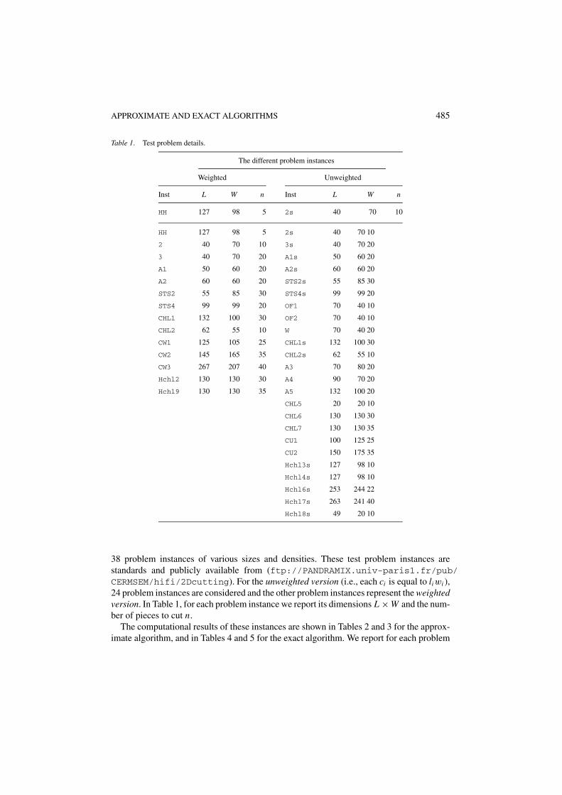
Table 1. Test problem details.

The different problem instances

Weighted Unweighted

Inst L W n Inst L W n

HH 127 98 5 2s 40 70 10

HH 127 98 5 2s 40 70 10

2 40 70 10 3s 40 70 20

3 40 70 20 A1s 50 60 20

A1 50 60 20 A2s 60 60 20

A2 60 60 20 STS2s 55 85 30

STS2 55 85 30 STS4s 99 99 20

STS4 99 99 20 OF1 70 40 10

CHL1 132 100 30 OF2 70 40 10

CHL2 62 55 10 W 70 40 20

CW1 125 105 25 CHL1s 132 100 30

CW2 145 165 35 CHL2s 62 55 10

CW3 267 207 40 A3 70 80 20

Hchl2 130 130 30 A4 90 70 20

Hchl9 130 130 35 A5 132 100 20

CHL5 20 20 10

CHL6 130 130 30

CHL7 130 130 35

CU1 100 125 25

CU2 150 175 35

Hchl3s 127 98 10

Hchl4s 127 98 10

Hchl6s 253 244 22

Hchl7s 263 241 40

Hchl8s 49 20 10

38 problem instances of various sizes and densities. These test problem instances arestandards and publicly available from (ftp://PANDRAMIX.univ-paris1.fr/pub/CERMSEM/hifi/2Dcutting). For the unweighted version (i.e., each ci is equal to liwi ),24 problem instances are considered and the other problem instances represent the weightedversion. In Table 1, for each problem instance we report its dimensions L × W and the num-ber of pieces to cut n.

The computational results of these instances are shown in Tables 2 and 3 for the approx-imate algorithm, and in Tables 4 and 5 for the exact algorithm. We report for each problem


instance (with and without trimming):

• The Approximate horizontal (resp. vertical) solution value (denoted Ahor, resp. Aver ),which represents a lower bound produced by the approximate algorithm (algorithm ofSection 3 when trimming is not permitted and algorithm of Section 4 otherwise).

• The Optimal horizontal (resp. vertical) solution value, denoted Opthor (resp. Optver ),reached by the exact algorithm. The optimal solution value, denoted Opt, when the firststage-cut is unspecified.

• The experimental Approximation Ratio (A.R.) obtained by applying the usual formulaA(I )

Opt(I ) , where I is an instance of the problem, H(I ) denotes the approximate solutionvalue and Opt(I ) is the optimal solution value.

• The Execution Time (E.T., measured in seconds) which is the time that the consideredapproximate (resp. exact) algorithm takes to reach the approximate (resp. optimal) hori-zontal or vertical solution.

• The number of generated nodes, denoted Nodes, when the exact algorithm is applied.

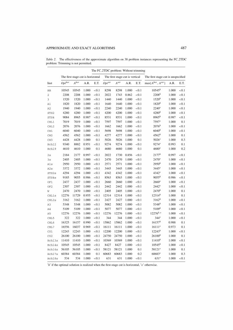
7.1. Performance of the approximate algorithms

Table 2 shows the behavior of the approximate algorithm when trimming is not permitted(Columns 4, 8 and 11 respectively). For all treated instances, excellent lower bounds areobtained. We remark that A.R.s are generally close to one, except for some instances:

– The first-cut is unspecified: the instances STS4, Hchl2, 2s, STS4s, CHL6 and CHL7,for which the A.R.s varie between 0.973 and 0.993.

– The first-cut is horizontal: the instances STS4, Hchl1, Hchl2, 2s, STS4s, CHL1s,CHL6 and CHL7 (the A.R.s are between 0.951 and 0.997).

– The first-cut is vertical: the instances 2 and 2s, which realizes A.R.s equal to 0.862 and0.856, respectivelly.

Also, we observe that the computational time is generally under 0.3 sec (Columns 5, 9 and12 respectively).

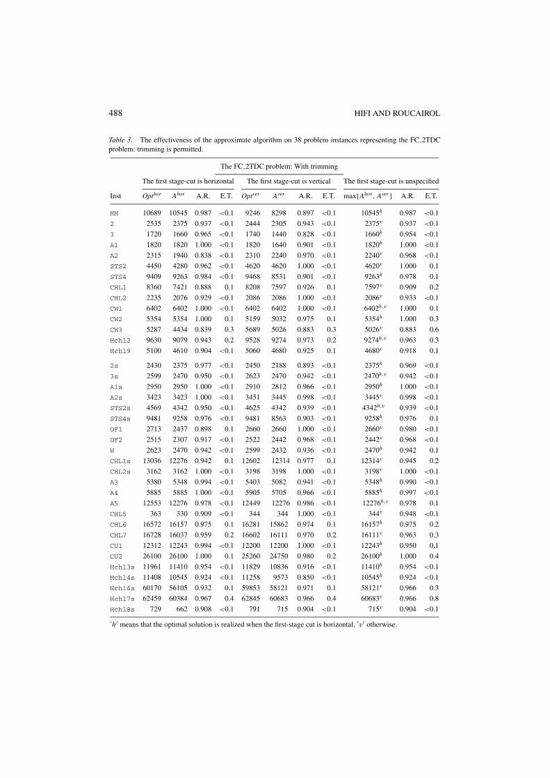
When trimming is permitted (see Table 3), the approximate algorithm produces:

– The first-cut is unspecified: an A.R. which varies between 0.883 (instance CW3) and 1(see Table 3, column 11) and by consuming less than 1 Sec.

– The first-cut is horizontal (resp. vertical): an A.R. which varies between 0.838 (instanceA2) (resp. 0.883 (instance CW3)) and 1 (see Table 3, column 4 (resp. column 8)) and byconsuming less than 1 Sec.

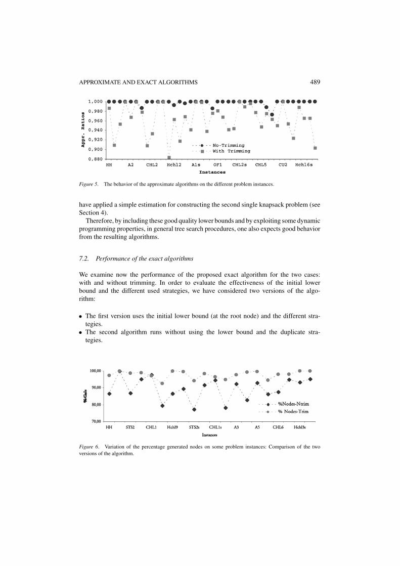
Figure 5 shows the different A.R.s produced by the approximate algorithm on the 38problem instances. It shows that it produces better A.R.s when trimming is not permitted.This can be explained by the fact that the single knapsack problems are solved separatelyand they are totally independent, which is not the case for the non-exact case: in this case,we have applied a simple greedy algorithm for solving each set packing problem or we


Table 2. The effectiveness of the approximate algorithm on 38 problem instances representing the FC 2TDCproblem: Trimming is not permitted.

The FC 2TDC problem: Without trimming

The first stage-cut is horizontal The first stage-cut is vertical The first stage-cut is unspecified

Inst Opthor Ahor A.R. E.T. Optver Aver A.R. E.T. max{Ahor, Aver } A.R. E.T.

HH 10545 10545 1.000 <0.1 8298 8298 1.000 <0.1 10545h 1.000 <0.1

2 2208 2208 1.000 <0.1 2022 1743 0.862 <0.1 2208h 1.000 <0.1

3 1520 1520 1.000 <0.1 1440 1440 1.000 <0.1 1520h 1.000 <0.1

A1 1820 1820 1.000 <0.1 1640 1640 1.000 <0.1 1820h 1.000 <0.1

A2 1940 1940 1.000 <0.1 2240 2240 1.000 <0.1 2240v 1.000 <0.1

STS2 4280 4280 1.000 <0.1 4200 4200 1.000 <0.1 4280h 1.000 <0.1

STS4 9084 8965 0.987 <0.1 8531 8531 1.000 <0.1 8965h 0.987 <0.1

CHL1 7019 7019 1.000 <0.1 7597 7597 1.000 <0.1 7597v 1.000 0.1

CHL2 2076 2076 1.000 <0.1 1662 1662 1.000 <0.1 2076h 1.000 <0.1

CW1 6040 6040 1.000 <0.1 5698 5698 1.000 <0.1 6040h 1.000 <0.1

CW2 4562 4562 1.000 <0.1 4277 4277 1.000 <0.1 4562h 1.000 0.1

CW3 4428 4428 1.000 0.1 5026 5026 1.000 0.1 5026v 1.000 0.3

Hchl2 9340 8882 0.951 <0.1 9274 9274 1.000 <0.1 9274v 0.993 0.1

Hchl9 4610 4610 1.000 0.1 4680 4680 1.000 0.1 4680v 1.000 0.2

2s 2184 2177 0.997 <0.1 2022 1730 0.856 <0.1 2177h 0.997 <0.1

3s 2405 2405 1.000 <0.1 2470 2470 1.000 <0.1 2470v 1.000 <0.1

A1s 2950 2950 1.000 <0.1 2571 2571 1.000 <0.1 2950h 1.000 <0.1

A2s 3372 3372 1.000 <0.1 3445 3445 1.000 <0.1 3445v 1.000 <0.1

STS2s 4294 4294 1.000 <0.1 4342 4342 1.000 <0.1 4342v 1.000 <0.1

STS4s 9185 9055 0.986 <0.1 8563 8563 1.000 <0.1 9055h 0.986 <0.1

OF1 2437 2437 1.000 <0.1 2660 2660 1.000 <0.1 2660v 1.000 <0.1

OF2 2307 2307 1.000 <0.1 2442 2442 1.000 <0.1 2442v 1.000 <0.1

W 2470 2470 1.000 <0.1 2405 2405 1.000 <0.1 2470h 1.000 0.1

CHL1s 12276 11729 0.955 <0.1 12314 12314 1.000 <0.1 12314h 1.000 0.1

CHL2s 3162 3162 1.000 <0.1 2427 2427 1.000 <0.1 3162h 1.000 <0.1

A3 5348 5348 1.000 <0.1 5082 5082 1.000 <0.1 5348h 1.000 <0.1

A4 5109 5109 1.000 <0.1 5077 5077 1.000 <0.1 5109h 1.000 <0.1

A5 12276 12276 1.000 <0.1 12276 12276 1.000 <0.1 12276h,v 1.000 <0.1

CHL5 322 322 1.000 <0.1 344 344 1.000 <0.1 344v 1.000 <0.1

CHL6 16325 16157 0.990 <0.1 15862 15862 1.000 <0.1 16157h 0.988 0.1

CHL7 16556 16037 0.969 <0.1 16111 16111 1.000 <0.1 16111v 0.973 0.1

CU1 12243 12243 1.000 <0.1 12200 12200 1.000 <0.1 12243h 1.000 <0.1

CU2 26100 26100 1.000 <0.1 24750 24750 1.000 <0.1 26100h 1.000 0.1

Hchl3s 11410 11410 1.000 <0.1 10369 10369 1.000 <0.1 11410h 1.000 <0.1

Hchl4s 10545 10545 1.000 <0.1 8427 8427 1.000 <0.1 10545h 1.000 <0.1

Hchl6s 56105 56105 1.000 <0.1 58121 58121 1.000 0.1 58121v 1.000 0.1

Hchl7s 60384 60384 1.000 0.1 60683 60683 1.000 0.2 60683v 1.000 0.3

Hchl8s 534 534 1.000 <0.1 631 631 1.000 <0.1 631v 1.000 <0.1

′h′ if the optimal solution is realized when the first-stage cut is horizontal, ′v′ otherwise.


Table 3. The effectiveness of the approximate algorithm on 38 problem instances representing the FC 2TDCproblem: trimming is permitted.

The FC 2TDC problem: With trimming


Inst Opthor Ahor A.R. E.T. Optver Aver A.R. E.T. max{Ahor, Aver } A.R. E.T.

HH 10689 10545 0.987 <0.1 9246 8298 0.897 <0.1 10545h 0.987 <0.1

2 2535 2375 0.937 <0.1 2444 2305 0.943 <0.1 2375v 0.937 <0.1

3 1720 1660 0.965 <0.1 1740 1440 0.828 <0.1 1660h 0.954 <0.1

A1 1820 1820 1.000 <0.1 1820 1640 0.901 <0.1 1820h 1.000 <0.1

A2 2315 1940 0.838 <0.1 2310 2240 0.970 <0.1 2240v 0.968 <0.1

STS2 4450 4280 0.962 <0.1 4620 4620 1.000 <0.1 4620v 1.000 0.1

STS4 9409 9263 0.984 <0.1 9468 8531 0.901 <0.1 9263h 0.978 0.1

CHL1 8360 7421 0.888 0.1 8208 7597 0.926 0.1 7597v 0.909 0.2

CHL2 2235 2076 0.929 <0.1 2086 2086 1.000 <0.1 2086v 0.933 <0.1

CW1 6402 6402 1.000 <0.1 6402 6402 1.000 <0.1 6402h,v 1.000 0.1

CW2 5354 5354 1.000 0.1 5159 5032 0.975 0.1 5354h 1.000 0.3

CW3 5287 4434 0.839 0.3 5689 5026 0.883 0.3 5026v 0.883 0.6

Hchl2 9630 9079 0.943 0.2 9528 9274 0.973 0.2 9274h,v 0.963 0.3

Hchl9 5100 4610 0.904 <0.1 5060 4680 0.925 0.1 4680v 0.918 0.1

2s 2430 2375 0.977 <0.1 2450 2188 0.893 <0.1 2375h 0.969 <0.1

3s 2599 2470 0.950 <0.1 2623 2470 0.942 <0.1 2470h,v 0.942 <0.1

A1s 2950 2950 1.000 <0.1 2910 2812 0.966 <0.1 2950h 1.000 <0.1

A2s 3423 3423 1.000 <0.1 3451 3445 0.998 <0.1 3445v 0.998 <0.1

STS2s 4569 4342 0.950 <0.1 4625 4342 0.939 <0.1 4342h,v 0.939 <0.1

STS4s 9481 9258 0.976 <0.1 9481 8563 0.903 <0.1 9258h 0.976 0.1

OF1 2713 2437 0.898 0.1 2660 2660 1.000 <0.1 2660v 0.980 <0.1

OF2 2515 2307 0.917 <0.1 2522 2442 0.968 <0.1 2442v 0.968 <0.1

W 2623 2470 0.942 <0.1 2599 2432 0.936 <0.1 2470h 0.942 0.1

CHL1s 13036 12276 0.942 0.1 12602 12314 0.977 0.1 12314v 0.945 0.2

CHL2s 3162 3162 1.000 <0.1 3198 3198 1.000 <0.1 3198v 1.000 <0.1

A3 5380 5348 0.994 <0.1 5403 5082 0.941 <0.1 5348h 0.990 <0.1

A4 5885 5885 1.000 <0.1 5905 5705 0.966 <0.1 5885h 0.997 <0.1

A5 12553 12276 0.978 <0.1 12449 12276 0.986 <0.1 12276h,v 0.978 0.1

CHL5 363 330 0.909 <0.1 344 344 1.000 <0.1 344v 0.948 <0.1

CHL6 16572 16157 0.975 0.1 16281 15862 0.974 0.1 16157h 0.975 0.2

CHL7 16728 16037 0.959 0.2 16602 16111 0.970 0.2 16111v 0.963 0.3

CU1 12312 12243 0.994 <0.1 12200 12200 1.000 <0.1 12243h 0.950 0.1

CU2 26100 26100 1.000 0.1 25260 24750 0.980 0.2 26100h 1.000 0.4

Hchl3s 11961 11410 0.954 <0.1 11829 10836 0.916 <0.1 11410h 0.954 <0.1

Hchl4s 11408 10545 0.924 <0.1 11258 9573 0.850 <0.1 10545h 0.924 <0.1

Hchl6s 60170 56105 0.932 0.1 59853 58121 0.971 0.1 58121v 0.966 0.3

Hchl7s 62459 60384 0.967 0.4 62845 60683 0.966 0.4 60683v 0.966 0.8

Hchl8s 729 662 0.908 <0.1 791 715 0.904 <0.1 715v 0.904 <0.1

′h′ means that the optimal solution is realized when the first-stage cut is horizontal, ′v′ otherwise.


Figure 5. The behavior of the approximate algorithms on the different problem instances.

have applied a simple estimation for constructing the second single knapsack problem (seeSection 4).

Therefore, by including these good quality lower bounds and by exploiting some dynamicprogramming properties, in general tree search procedures, one also expects good behaviorfrom the resulting algorithms.

7.2. Performance of the exact algorithms

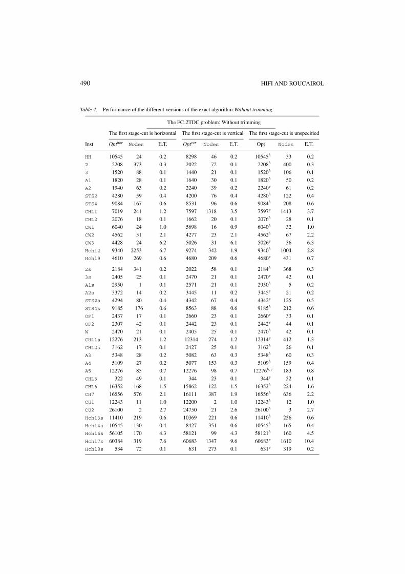
We examine now the performance of the proposed exact algorithm for the two cases:with and without trimming. In order to evaluate the effectiveness of the initial lowerbound and the different used strategies, we have considered two versions of the algo-rithm:

• The first version uses the initial lower bound (at the root node) and the different stra-tegies.

• The second algorithm runs without using the lower bound and the duplicate stra-tegies.

Figure 6. Variation of the percentage generated nodes on some problem instances: Comparison of the twoversions of the algorithm.


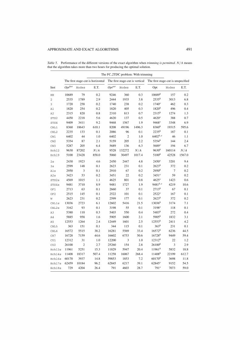
Table 4. Performance of the different versions of the exact algorithm:Without trimming.

The FC 2TDC problem: Without trimming


Inst Opthor Nodes E.T. Optver Nodes E.T. Opt Nodes E.T.

HH 10545 24 0.2 8298 46 0.2 10545h 33 0.2

2 2208 373 0.3 2022 72 0.1 2208h 400 0.3

3 1520 88 0.1 1440 21 0.1 1520h 106 0.1

A1 1820 28 0.1 1640 30 0.1 1820h 50 0.2

A2 1940 63 0.2 2240 39 0.2 2240v 61 0.2

STS2 4280 59 0.4 4200 76 0.4 4280h 122 0.4

STS4 9084 167 0.6 8531 96 0.6 9084h 208 0.6

CHL1 7019 241 1.2 7597 1318 3.5 7597v 1413 3.7

CHL2 2076 18 0.1 1662 20 0.1 2076h 28 0.1

CW1 6040 24 1.0 5698 16 0.9 6040h 32 1.0

CW2 4562 51 2.1 4277 23 2.1 4562h 67 2.2

CW3 4428 24 6.2 5026 31 6.1 5026v 36 6.3

Hchl2 9340 2253 6.7 9274 342 1.9 9340h 1004 2.8

Hchl9 4610 269 0.6 4680 209 0.6 4680v 431 0.7

2s 2184 341 0.2 2022 58 0.1 2184h 368 0.3

3s 2405 25 0.1 2470 21 0.1 2470v 42 0.1

A1s 2950 1 0.1 2571 21 0.1 2950h 5 0.2

A2s 3372 14 0.2 3445 11 0.2 3445v 21 0.2

STS2s 4294 80 0.4 4342 67 0.4 4342v 125 0.5

STS4s 9185 176 0.6 8563 88 0.6 9185h 212 0.6

OF1 2437 17 0.1 2660 23 0.1 2660v 33 0.1

OF2 2307 42 0.1 2442 23 0.1 2442v 44 0.1

W 2470 21 0.1 2405 25 0.1 2470h 42 0.1

CHL1s 12276 213 1.2 12314 274 1.2 12314v 412 1.3

CHL2s 3162 17 0.1 2427 25 0.1 3162h 26 0.1

A3 5348 28 0.2 5082 63 0.3 5348h 60 0.3

A4 5109 27 0.2 5077 153 0.3 5109h 159 0.4

A5 12276 85 0.7 12276 98 0.7 12276h,v 183 0.8

CHL5 322 49 0.1 344 23 0.1 344v 52 0.1

CHL6 16352 168 1.5 15862 122 1.5 16352h 224 1.6

CH7 16556 576 2.1 16111 387 1.9 16556h 636 2.2

CU1 12243 11 1.0 12200 2 1.0 12243h 12 1.0

CU2 26100 2 2.7 24750 21 2.6 26100h 3 2.7

Hchl3s 11410 219 0.6 10369 221 0.6 11410h 256 0.6

Hchl4s 10545 130 0.4 8427 351 0.6 10545h 165 0.4

Hchl6s 56105 170 4.3 58121 99 4.3 58121h 160 4.5

Hchl7s 60384 319 7.6 60683 1347 9.6 60683v 1610 10.4

Hchl8s 534 72 0.1 631 273 0.1 631v 319 0.2


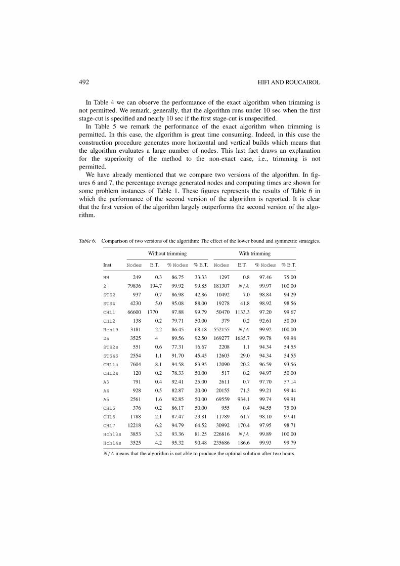
Table 5. Performance of the different versions of the exact algorithm when trimming is permitted. N/A meansthat the algorithm takes more than two hours for producing the optimal solution.

The FC 2TDC problem: With trimming


Inst Opthor Nodes E.T. Optver Nodes E.T. Opt Nodes E.T.

HH 10689 79 0.2 9246 360 0.3 10689h 157 0.2

2 2535 1789 2.9 2444 1935 3.8 2535h 3013 6.8

3 1720 258 0.2 1740 238 0.2 1740v 462 0.3

A1 1820 254 0.2 1820 405 0.3 1820h 496 0.4

A2 2315 820 0.8 2310 813 0.7 2315h 1274 1.3

STS2 4450 2218 5.6 4620 137 0.5 4620v 388 0.7

STS4 9409 3411 9.2 9468 1567 1.9 9468v 3348 6.9

CHL1 8360 18643 610.1 8208 49196 1496.3 8360h 19315 595.6

CHL2 2235 133 0.1 2086 96 0.1 2235h 187 0.1

CW1 6402 44 1.0 6402 2 1.0 6402h,v 46 1.1

CW2 5354 87 2.1 5159 205 2.2 5354h 144 2.4

CW3 5287 205 6.4 5689 136 6.3 5689v 194 6.7

Hchl2 9630 87202 N/A 9528 132272 N/A 9630h 160114 N/A

Hchl9 5100 23428 858.0 5060 30497 1017.4 5100h 42528 1567.0

2s 2430 1923 4.6 2450 2447 4.8 2450v 3201 9.4

3s 2599 148 0.1 2623 231 0.1 2623h 372 0.2

A1s 2950 3 0.1 2910 67 0.2 2950h 7 0.2

A2s 3423 53 0.2 3451 22 0.2 3451v 59 0.2

STS2s 4569 1015 1.1 4625 801 0.8 4625v 1423 0.6

STS4s 9481 3710 8.9 9481 1727 1.9 9481h,v 4219 10.6

OF1 2713 63 0.1 2660 37 0.1 2713h 67 0.1

OF2 2515 145 0.1 2522 101 0.1 2522v 167 0.1

W 2623 231 0.2 2599 177 0.1 2623h 372 0.2

CHL1s 13036 2723 6.1 12602 5416 21.5 13036h 3174 7.1

CHL2s 3162 93 0.1 3198 55 0.1 3198v 118 0.1

A3 5380 110 0.3 5403 550 0.4 5403h 272 0.4

A4 5885 958 1.6 5905 1600 2.1 5905h 1832 3.1

A5 12553 1264 2.4 12449 1601 2.5 12553h 2411 4.2

CHL5 363 151 0.1 344 115 0.1 363h 231 0.1

CHL6 16572 5515 38.2 16281 5569 33.4 16572h 6236 44.5

CH7 16728 7159 44.6 16602 6753 50.6 16728h 9449 59.4

CU1 12312 31 1.0 12200 3 1.0 12312h 22 1.2

CU2 26100 2 2.7 25260 154 2.8 26100h 3 2.9

Hchl3s 11961 5251 15.3 11829 5947 20.4 11961h 5832 18.8

Hchl4s 11408 18317 507.4 11258 16067 268.4 11408h 22199 612.7

Hchl6s 60170 3937 14.8 59853 1853 7.2 60170h 3698 11.8

Hchl7s 62459 10184 96.2 62845 6217 39.1 62845v 9152 54.5

Hchl8s 729 4204 26.4 791 4603 28.7 791v 7073 59.0


In Table 4 we can observe the performance of the exact algorithm when trimming isnot permitted. We remark, generally, that the algorithm runs under 10 sec when the firststage-cut is specified and nearly 10 sec if the first stage-cut is unspecified.

In Table 5 we remark the performance of the exact algorithm when trimming ispermitted. In this case, the algorithm is great time consuming. Indeed, in this case theconstruction procedure generates more horizontal and vertical builds which means thatthe algorithm evaluates a large number of nodes. This last fact draws an explanationfor the superiority of the method to the non-exact case, i.e., trimming is notpermitted.

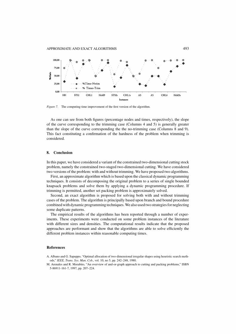
We have already mentioned that we compare two versions of the algorithm. In fig-ures 6 and 7, the percentage average generated nodes and computing times are shown forsome problem instances of Table 1. These figures represents the results of Table 6 inwhich the performance of the second version of the algorithm is reported. It is clearthat the first version of the algorithm largely outperforms the second version of the algo-rithm.

Table 6. Comparison of two versions of the algorithm: The effect of the lower bound and symmetric strategies.

Without trimming With trimming

Inst Nodes E.T. % Nodes % E.T. Nodes E.T. % Nodes % E.T.

HH 249 0.3 86.75 33.33 1297 0.8 97.46 75.00

2 79836 194.7 99.92 99.85 181307 N/A 99.97 100.00

STS2 937 0.7 86.98 42.86 10492 7.0 98.84 94.29

STS4 4230 5.0 95.08 88.00 19278 41.8 98.92 98.56

CHL1 66600 1770 97.88 99.79 50470 1133.3 97.20 99.67

CHL2 138 0.2 79.71 50.00 379 0.2 92.61 50.00

Hchl9 3181 2.2 86.45 68.18 552155 N/A 99.92 100.00

2s 3525 4 89.56 92.50 169277 1635.7 99.78 99.98

STS2s 551 0.6 77.31 16.67 2208 1.1 94.34 54.55

STS4S 2554 1.1 91.70 45.45 12603 29.0 94.34 54.55

CHL1s 7604 8.1 94.58 83.95 12090 20.2 96.59 93.56

CHL2s 120 0.2 78.33 50.00 517 0.2 94.97 50.00

A3 791 0.4 92.41 25.00 2611 0.7 97.70 57.14

A4 928 0.5 82.87 20.00 20155 71.3 99.21 99.44

A5 2561 1.6 92.85 50.00 69559 934.1 99.74 99.91

CHL5 376 0.2 86.17 50.00 955 0.4 94.55 75.00

CHL6 1788 2.1 87.47 23.81 11789 61.7 98.10 97.41

CHL7 12218 6.2 94.79 64.52 30992 170.4 97.95 98.71

Hchl3s 3853 3.2 93.36 81.25 226816 N/A 99.89 100.00

Hchl4s 3525 4.2 95.32 90.48 235686 186.6 99.93 99.79

N/A means that the algorithm is not able to produce the optimal solution after two hours.


Figure 7. The computing time improvement of the first version of the algorithm.

As one can see from both figures (percentage nodes and times, respectively), the slopeof the curve corresponding to the trimming case (Columns 4 and 5) is generally greaterthan the slope of the curve corresponding the the no-trimming case (Columns 8 and 9).This fact constituting a confirmation of the hardness of the problem when trimming isconsidered.

8. Conclusion

In this paper, we have considered a variant of the constrained two-dimensional cutting stockproblem, namely the constrained two-staged two-dimensional cutting. We have consideredtwo versions of the problem: with and without trimming. We have proposed two algorithms.

First, an approximate algorithm which is based upon the classical dynamic programmingtechniques. It consists of decomposing the original problem to a series of single boundedknapsack problems and solve them by applying a dynamic programming procedure. Iftrimming is permitted, another set packing problem is approximately solved.

Second, an exact algorithm is proposed for solving both with and without trimmingcases of the problem. The algorithm is principally based upon branch and bound procedurecombined with dynamic programming techniques. We also used two strategies for neglectingsome duplicate patterns.

The empirical results of the algorithms has been reported through a number of exper-iments. These experiments were conducted on some problem instances of the literaturewith different sizes and densities. The computational results indicate that the proposedapproaches are performant and show that the algorithms are able to solve efficiently thedifferent problem instances within reasonable computing times.

References

A. Albano and G. Sapuppo, “Optimal allocation of two-dimensional irregular shapes using heuristic search meth-ods,” IEEE, Trans. Sys. Man. Cyb., vol. 10, no 5, pp. 242–248, 1980.

M. Arenales and R. Morabito, “An overview of and-or-graph approach to cutting and packing problems,” ISBN5-86911-161-7, 1997, pp. 207–224.


J.E. Beasley, “Algorithms for unconstrained two-dimensional guillotine cutting,” Journal of the OperationalResearch Society, vol. 36, pp. 297–306, 1985.

N. Christofides and E. Hadjiconstantinou, “An exact algorithm for orthogonal 2-D cutting problems using guillotinecuts,” European Journal of Operational Research, vol. 83, pp. 21–38, 1995.

N. Christofides and C. Whitlock, “An algorithm for two-dimensional cutting problems,” Operations Research,vol. 2, pp. 31–44, 1977.

V-D. Cung, M. Hifi, and B. Le Cun, “Constrained two-dimensional cutting stock problems: A best-first branch-and-bound algorithm,” International Transactions in Operational Research, vol. 7, pp. 185–210, 2000.

H. Dyckhoff, “A typology of cutting and packing problems,” European Journal of Operational Research, vol. 44,pp. 145–159, 1990.

D. Fayard, M. Hifi, and V. Zissimopoulos, “An efficient approach for large-scale two-dimensional guillotine cuttingstock problems,” Journal of the Operational Research Society, vol. 49, pp. 1270–1277, 1998.

P.C. Gilmore, “Cutting stock, linear programming, knapsacking, dynamic programming and integer programming,some interconnections,” Annals of Discrete Mathematics, vol. 4, pp. 217–235, 1979.

P.C. Gilmore and R.E. Gomory, “Multistage cutting problems of two and more dimensions,” Operations Research,vol. 13, pp. 94–119, 1965.

P.C. Gilmore and R.E. Gomory, “The theory and computation of knapsack functions,” Operations Research, vol.14, pp. 1045–1074, 1966.

J.C. Herz, “A recursive computing procedure for two-dimensional stock cutting,” IBM Journal of Research andDevelopment, vol. 16, pp. 462–469, 1972.

M. Hifi, “An improvement of Viswanathan and Bagchi’s exact algorithm for cutting stock problems,” Computersand Operations Research, vol. 24, pp.727–736, 1997.

M. Hifi, “Contribution a la resolution de quelques problemes difficiles de l’optimisation combinatoire,” HabilitationThesis. PRiSM, Universite de Versailles St-Quentin en Yvelines, 1999.

M. Hifi, “Exact algorithms for large-scale unconstrained two and three staged cutting problems,” ComputationalOptimization and Applications, vol. 18, pp. 63–88, 2001.

M. Hifi and V. Zissimopoulos, “A recursive exact algorithm for weighted two-dimensional cutting problems,”European Journal of Operational Research, vol. 91, pp. 553–564, 1996.

M. Hifi and V. Zissimopoulos, “Constrained two-dimensional cutting: An improvement of Christofides and Whit-lock’s exact algorithm,” Journal of the Operational Research Society, vol. 5, pp. 8–18, 1997.

E.L. Lawler, “Fast approximation algorithms for knapsack problems,” Mathematics of Operations Research, vol.4, pp. 339–356, 1979.

S. Martello and P. Toth, “An exact algorithm for large unbounded knapsack problems,” Operations ResearchLetters, vol. 9, pp. 15–20, 1990.

S. Martello and P. Toth, “Upper bounds and algorithms for hard 0-1 knapsack problems,” Operations Research,vol. 45, pp. 768–778, 1997.

R. Morabito and M. Arenales, “Staged and constrained two-dimensional guillotine cutting problems: An and-or-graph approach,” European Journal of Operational Research, vol. 94, no. 3, pp. 548–560, 1996.

R. Morabito, M. Arenales, and V. Arcaro, “An and-or-graph approach for two-dimensional cutting problems,”European Journal of Operational Research, vol. 58, no. 2, pp. 263–271, 1992.

R. Morabito and V. Garcia, “The cutting stock problem in hardboard industry: A case study,” Computers andOperations Research, vol. 25, pp. 469–485, 1998.

D. Pisinger, “A minimal algorithm for the 0-1 knapsack problem,” Operations Research, vol. 45, pp. 758–767,1997.

P.E. Sweeney and E.R. Paternoster, “Cutting and packing problems: A categorized applications-oriented researchbibliography,” Journal of the Operational Research Society, vol. 43, pp. 691–706, 1992.

M. Syslo, N. Deo, and J. Kowalik, Discrete Optimization Algorithms, Prentice-Hall: New Jersey, 1983.K.V. Viswanathan and A. Bagchi, “Best-first search methods for constrained two-dimensional cutting stock prob-

lems,” Operations Research, vol. 41, no. 4, pp. 768–776, 1993.P.Y. Wang, “Two algorithms for constrained two-dimensional cutting stock problems,” Operations Research, vol.

31, no. 3, pp. 573–586, 1983.

approximate and exact algorithms for constrained (un) weighted two-dimensional two-staged cutting...

Documents