approaches for selecting bmps and estimating their performance · approaches for selecting bmps and...
TRANSCRIPT

1
Approaches for Selecting BMPs and EstimatingTheir Performance
Stephen Carter, PE
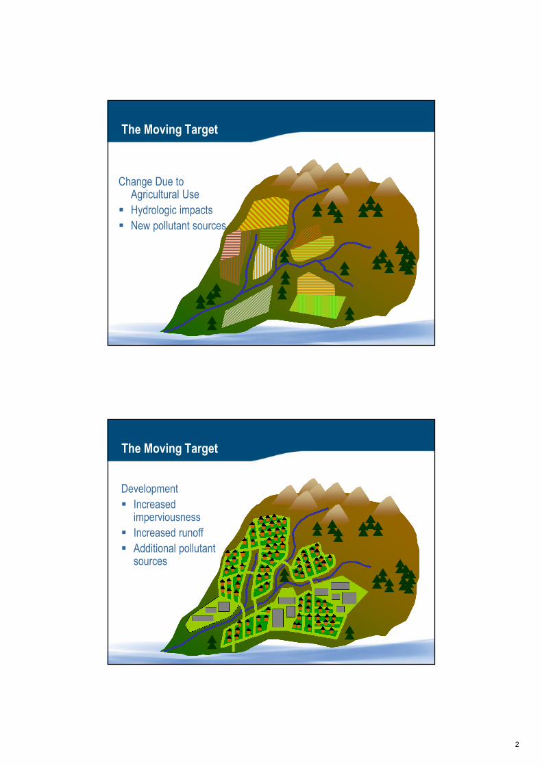
The Moving Target
Starting point
Reference condition
Naturally evolvedstream condition
2
The Moving Target
Change Due toAgricultural Use
Hydrologic impacts
New pollutant sources
The Moving Target
Development
Increasedimperviousness
Increased runoff
Additional pollutantsources

3
Typical Trend
De
gra
da
tion
Ma
na
ge
me
ntA
ctio
ns
WaterQuality
Degradation
ManagementActions
BMPs
ChangingBehaviors
SmartGrowth
What’s the Goal?
De
gra
da
tion
Target
Water quality criteria
Reference watershedcondition
TMDL
Ma
na
ge
me
ntA
ctio
ns
Existing Condition
Water quality
Pollutant load

4
De
gra
da
tion M
an
ag
em
en
tActio
ns Components of the
Watershed Plan
Specificmanagement actions
Pollutant loadreduction
Improved waterquality
What’s the Goal?
< 1 – 10 Acres: LID (Rain Barrels, Bioretention)
10 – 100 Acres: Grassed Swales,Ponds
> 100 Acres: RegionalFacilities,
Stream Restoration
TMDL
10,000s or100,000sActivities
Result inLoadReduction
Bo
ttom
–U
p
To
p–
Do
wn
Structural BMPs
5
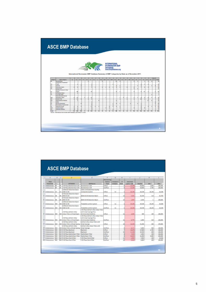
ASCE BMP Database
9
ASCE BMP Database
10
6
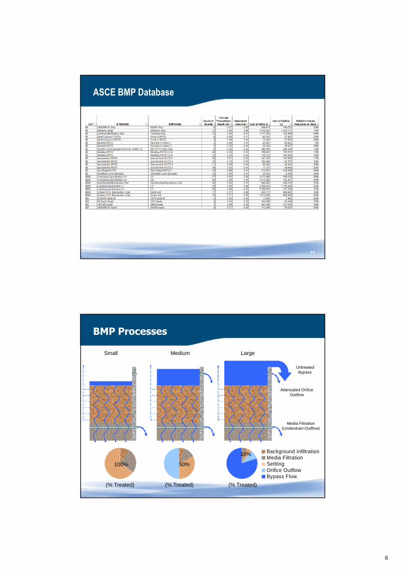
ASCE BMP Database
11
BMP Processes
Background InfiltrationMedia FiltrationSettlingOrifice OutflowBypass Flow
Small Medium
UntreatedBypass
Attenuated OrificeOutflow
Media Filtration(Underdrain Outflow)
Large
100%
(% Treated)
50%
(% Treated)
10%
(% Treated)

7
BMP Decision Support System (BMPDSS)
Prince George’s County, MDNational leader in stormwater and watershedmanagement – one of the most innovative andhighly reference programs in the country
Highlights: Basis for national strategies to address
stormwater challenges First and most referenced LID
guidance and design manuals Developed the BMP Decision
Support System (BMPDSS)
BMPDSS Interface
BMPDSS Set Up
BMPDSS Output:BMP Optimization
BMP Decision Support System (BMPDSS)
14

8
BMP Class A: Storage/Detention
OverflowSpillway
BottomOrifice
Evapotranspiration
Infiltration
Outflow:Inflow:
Modified Flow &Water Quality
From Land Surface
Storage
UnderdrainOutflow
Process-Based. Continuous Simulation.
BMP Class B: Open Channel
Outflow:Inflow:
From Land Surface
Overflow atMax Design
Depth
Open Channel Flow
Evapotranspiration
InfiltrationUnderdrain Outflow
Modified Flow &Water Quality
Process-Based. Continuous Simulation.

9
BMP Performance Curve Concept
Performed for EPA Region 10
BMPs curves developed fromcalibrated models and detailedperformance data
Provides long-term cumulativeperformance estimates basedon BMP capacity
Eliminates the need for detailedmodeling and evaluation inindividual applications 0%
10%
20%
30%
40%
50%
60%
70%
80%
90%
0.25 0.75 1.25 1.75 2.25
BMP size (controlled depth of runoff)
Pe
rce
nta
ge
rem
ov
al
for
TS
S
40%
0.65 in
0.90 in
BMP I
BMP II
Land simulation(SWMM)
Surface runoff generationand pollutant wash off
BMP simulation(BMPDSS)BMP Treatment
Precipitation
BMP Performance Curve Development Scheme
BMP Performance Curve: Gravel Wetland
Land Use: Commercial
0%
10%
20%
30%
40%
50%
60%
70%
80%
90%
100%
0 0.2 0.4 0.6 0.8 1 1.2 1.4 1.6 1.8 2
Depth of Runoff Treated (inches)
Po
llu
tan
tR
em
ov
al
TSS TP Zn

10
BMPDSS Calibration for Event 1/12/2006:Hydrology
0
50
100
150
200
2501
9:0
0
19
:40
20
:20
21
:00
21
:40
22
:20
23
:00
23
:40
0:2
0
1:0
0
1:4
0
2:2
0
3:0
0
3:4
0
4:2
0
5:0
0
5:4
0
6:2
0
7:0
0
7:4
0
8:2
0
9:0
0
9:4
0
10
:20
11
:00
Time
Flo
w(g
pm
)
Observed inflow
Generated inflow to infiltration system
Observed outflow
Calibrated BMPDSS outflow
BMPDSS Calibration: Water Quality
PollutantsCalibration events TSS TP Zn
Inflow 72.13 0.16 0.11ObservedEMC (mg/L) Outflow 0.17 0.03 0
Calibratedoutflow
0.17 0.03 0.006
Decay 0.76 0.31 0.4708/13/2005
BMPDSSperformance
Perct.removal
0.93 0.70 0.85
Inflow 52.06 0.10 0.03ObservedEMC (mg/L) Outflow 0 0.01 0
Calibratedoutflow
0.03 0.01 0.001
Decay 0.73 0.29 0.4401/12/2006
BMPDSSperformance
Perct.removal
0.90 0.65 0.81
Inflow 94.03 0.12 0.04ObservedEMC (mg/L) Outflow 0 0.02 0
Calibratedoutflow
0.01 0.02 0
Decay 0.73 0.21 0.4405/09/2006
BMPDSSperformance
Perct.removal
0.91 0.50 0.79
Decay 0.74 0.27 0.45Calibrated parameters Perct.
removal0.91 0.62 0.82

11
BMP Representation in BMPDSS
Generation of BMP Performance Curves
Commercial
Industrial
High-densityresidential
Medium-densityresidential
Low-densityresidential
Land uses(5)
Infiltration basin(6 infiltration rates)
Infiltration trenches(6 infiltration rates)
Bio-retention
Porous pavement
WQ Swales
Extended dry detention
Wet pond
Gravel wetland
BMPs(8) Pollutants
TSS
TP
Zn
Pollutants(3)
90 Figures and 282 Curves in total

12
Infiltration Trench
BMP Performance Curve: Infiltration Trench
Land Use: Industrial
(Soil Infiltration Rate 0.52 in/hr)
0%
10%
20%
30%
40%
50%
60%
70%
80%
90%
100%
0 0.2 0.4 0.6 0.8 1 1.2 1.4 1.6 1.8 2
Depth of Runoff Treated (inches)
Polluta
ntR
em
oval
0%
10%
20%
30%
40%
50%
60%
70%
80%
90%
100%
Runoff
Volu
me
Reduction
TSS TP Zn Volume
Infiltration Trench

13
Wet Pond
Wet PondB M P P e rfo rm an c e C u rve : W et P o nd
L an d U se : C o m m e rcial
0%
1 0%
2 0%
3 0%
4 0%
5 0%
6 0%
7 0%
8 0%
9 0%
1 0 0%
0 0.2 0 .4 0 .6 0.8 1 1.2 1 .4 1 .6 1.8 2
D e pt h of R u no ff T re at e d ( in ch e s )
Po
llu
tan
tR
em
ov
al
TS S TP Zn

14
Curve Extrapolation Tool
BMP Scale Considerations
SiteRegional

15
Lake Tahoe
Decline of Lake Tahoe Clarity
UC DavisTahoe Environmental Research Center

16
Pollutant Load Budget
Urban
Forested
AtmosphericDeposition
StreamChannelErosion
Groundwater
ShorelineErosion
15%
16%
54%
13%
Total Nitrogen
Pollutant Load Budget:
TotalPhosphorus
Urban
Forested
AtmosphericDeposition
StreamChannelErosion
Groundwater
ShorelineErosion
38%
26%
15%
15%
17
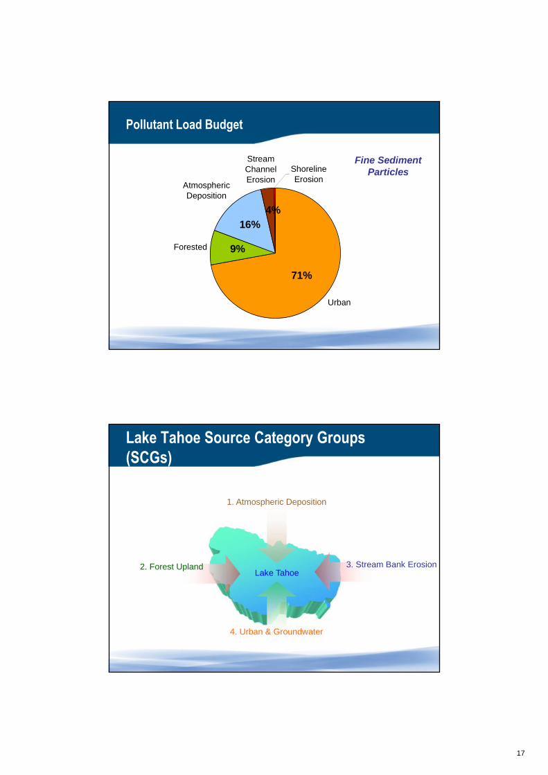
Pollutant Load Budget
Fine SedimentParticles
Urban
Forested
AtmosphericDeposition
StreamChannelErosion
ShorelineErosion
71%
9%
16%
4%
Lake Tahoe Source Category Groups(SCGs)
3. Stream Bank ErosionLake Tahoe
1. Atmospheric Deposition
4. Urban & Groundwater
2. Forest Upland
18
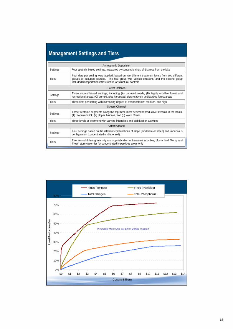
Atmospheric Deposition
Settings Four spatially based settings, measured by concentric rings of distance from the lake
TiersFour tiers per setting were applied, based on two different treatment levels from two differentgroups of pollutant sources. The first group was vehicle emisions, and the second groupincluded transportation infrastructure or structural controls
Forest Uplands
SettingsThree source based settings, including (A) unpaved roads, (B) highly erodible forest andrecreational areas, (C) burned, plus harvested, plus relatively undisturbed forest areas
Tiers Three tiers per setting with increasing degree of treatment: low, medium, and high
Stream Channel
SettingsThree treatable segments along the top three most sediment-productive streams in the Basin:(1) Blackwood Ck, (2) Upper Truckee, and (3) Ward Creek
Tiers Three levels of treatment with varying intensities and stabilization activities
Urban Upland
SettingsFour settings based on the different combinations of slope (moderate or steep) and imperviousconfiguration (concentrated or dispersed).
TiersTwo tiers of differing intensity and sophistication of treatment activities, plus a third "Pump andTreat" stormwater tier for concentrated impervious areas only
Management Settings and Tiers
0%
10%
20%
30%
40%
50%
60%
70%
80%
$0 $1 $2 $3 $4 $5 $6 $7 $8 $9 $10 $11 $12 $13 $14
Cost ($ Billion)
Lo
ad
Red
ucti
on
(%)
Fines (Tonnes) Fines (Particles)
Total Nitrogen Total Phosphorus
Theoretical Maximums per Billion Dollars Invested

19
Agua Hedionda Watershed Management Plan
Unincorp.Area
Unincorp.Area
78
Carlsbad
Oceanside
Vista
San Marcos
I-5
SR-76 EB
I-5
78
EL CAM REAL
SUNSET DR
TAMARACK AV
CA
RLS
BA
DB
L PO
INSETT
IAAV
SY
CA
MO
RE
AV
MARVIS
TADR
BUENACREEK
RD
LAKE BL
SSAN
TAFE
AV
0 1 20.5Kilometers
0 0.9 1.80.45Miles
Agua Hedionda - Modeling SubwateshedsNAD_1983_StatePlane_California_VI_FIPS_0406_Feet
Map produced 03-24-2008 - Peter Cada
Legend
Subwatersheds
Streams
Water
Roads
20
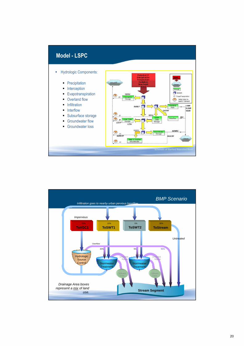
Model - LSPC
Hydrologic Components:
Precipitation
Interception
Evapotranspiration
Overland flow
Infiltration
Interflow
Subsurface storage
Groundwater flow
Groundwater loss
Schematic of Stanford Watershed Model
Stream Segment
StormwaterTreatment
2EffluentConc.
UntreatedBypass
StormwaterTreatment
1EffluentConc.
UntreatedBypass
Overflow
Infiltration goes to nearby urban pervious baseflow
Drainage Area boxesrepresent a mix of land
use.
Untreated
HydrologicSourceControl
Impervious
ToSWT1ToHSC1 ToSWT2 ToStream
55%5%40%
55% 30%10% 5%
BMP Scenario
21
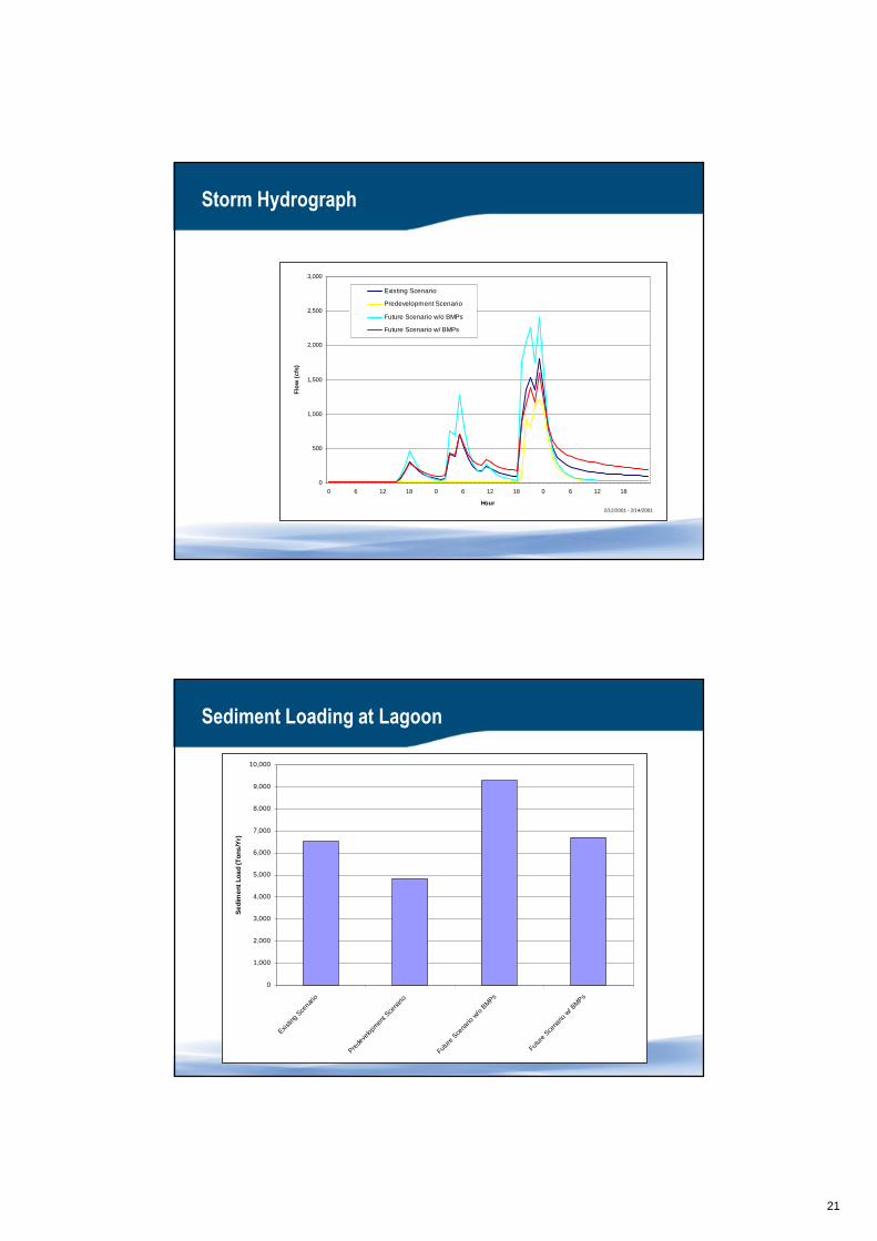
Storm Hydrograph
0
500
1,000
1,500
2,000
2,500
3,000
0 6 12 18 0 6 12 18 0 6 12 18
Hour
Flo
w(c
fs)
Existing Scenario
Predevelopment Scenario
Future Scenario w/o BMPs
Future Scenario w/ BMPs
2/12/2001 - 2/14/2001
Sediment Loading at Lagoon
0
1,000
2,000
3,000
4,000
5,000
6,000
7,000
8,000
9,000
10,000
Existing
Scena
rio
Prede
velopm
ent S
cena
rio
Futu
reSce
nario
w/oBM
Ps
Futu
reSce
nario
w/ BM
Ps
Se
dim
en
tL
oa
d(T
on
s/Y
r)

22
City of San Diego Evaluation of Structural andNonstructural BMP Performance
Chollas CreekWatershed
LSPC Model
Suspendedsediment
Trace metals• Copper
• Lead
• Zinc
Bacteria
43
Chollas Creek WatershedReaches Used in Model
0 1 2 30.5
Km
0 0.6 1.20.3Mi
NAD_1983_StatePlane_California_VI_FIPS_0406_FeetMap Produced 10/27/2009 by E. Moreno
Legend
Streams
Chollas Watershed
Modeling Scenarios
Long-term simulations (e.g., 10 years)
Capture a range of conditions
Scenarios
Current conditions• Baseline scenario for comparison
Management scenarios• Individual BMPs
• Combinations
44

23
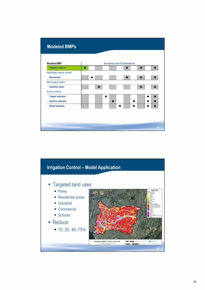
Modeled BMPs
Modeled BMP Scenarios and Combinations
Irrigation control ● ● ● ●Hydrologic source control
Bioretention ● ● ● ●Stormwater control
Detention basin ● ● ●Source control
Copper reduction ● ● ●Bacteria reduction ● ● ● ●Street sweeping ● ● ● ●
45
BMP Representation within a Watershed Model
LSPC does not include explicit representation of individualBMPs
Assumptions are developed to represent BMPs
Modeling assumptions can be based on
Specified BMP operational or design requirements
BMP literature information
Special studies on BMP performance
46

24
Source Control
Reach Outflow
Storm Drain Reach
Time
Ru
no
ff
Lower PollutantLevels
Time
Ru
no
ff
Pollutant Buildup
Land UseParcel
Time
Po
lluta
nt
Le
vel
47
Source Control
Examples
Reduced irrigation, treet sweeping, brake padmodification, pet BMPs
48
25
Modeled BMPs
Modeled BMP Scenarios and Combinations
Irrigation control ● ● ● ●Hydrologic source control
Bioretention ● ● ● ●Stormwater control
Detention basin ● ● ●Source control
Copper reduction ● ● ●Bacteria reduction ● ● ● ●Street sweeping ● ● ● ●
49
Irrigation Control – Model Application
Targeted land uses Parks
Residential areas
Industrial
Commercial
Schools
Reduce
10, 20, 40, 75%
50
Land UseAgricultureCommercialHealthCareSchoolPublicCemeteryGolfLandscapeOpenOpenRecParkMobileHomeParksMultiFamilyResidentialSingleFamilyResidentialSpacedRuralResidentialFreewayRoadMilitaryParkingIndustrialTrainTransportationWarehousingPublicStorageWater
0 1 20.5
Kilometers
0 1 20.5
Miles
Targeted Irrigation Control Land UsesNAD_1927_StatePlane_California_VI_FIPS_0405_feet
Map produced 03-18-2010

26
Irrigation Control – Monthly Reductions
51
-100%
-90%
-80%
-70%
-60%
-50%
-40%
-30%
-20%
-10%
0%
Oct
ob
er
No
vem
be
r
De
cem
be
r
Jan
uar
y
Feb
ruar
y
Mar
ch
Ap
ril
May
Jun
e
July
Au
gust
Sep
tem
be
r
Vo
lum
e
-100%
-90%
-80%
-70%
-60%
-50%
-40%
-30%
-20%
-10%
0%
Oct
ob
er
No
vem
be
r
De
cem
be
r
Jan
uar
y
Feb
ruar
y
Mar
ch
Ap
ril
May
Jun
e
July
Au
gust
Sep
tem
be
r
Co
pp
er
-100%
-90%
-80%
-70%
-60%
-50%
-40%
-30%
-20%
-10%
0%
Oct
ob
er
No
vem
be
r
De
cem
be
r
Jan
uar
y
Feb
ruar
y
Mar
ch
Ap
ril
May
Jun
e
July
Au
gust
Sep
tem
be
r
Feca
lCo
lifo
rm
-100%
-90%
-80%
-70%
-60%
-50%
-40%
-30%
-20%
-10%
0%
Oct
ob
er
No
vem
be
r
De
cem
be
r
Jan
uar
y
Feb
ruar
y
Mar
ch
Ap
ril
May
Jun
e
July
Au
gust
Sep
tem
be
r
Sed
ime
nt
Modeled BMPs
Modeled BMP Scenarios and Combinations
Irrigation control ● ● ● ●Hydrologic source control
Bioretention ● ● ● ●Stormwater control
Detention basin ● ● ●Source control
Copper reduction ● ● ●Bacteria reduction ● ● ● ●Street sweeping ● ● ● ●
52
27
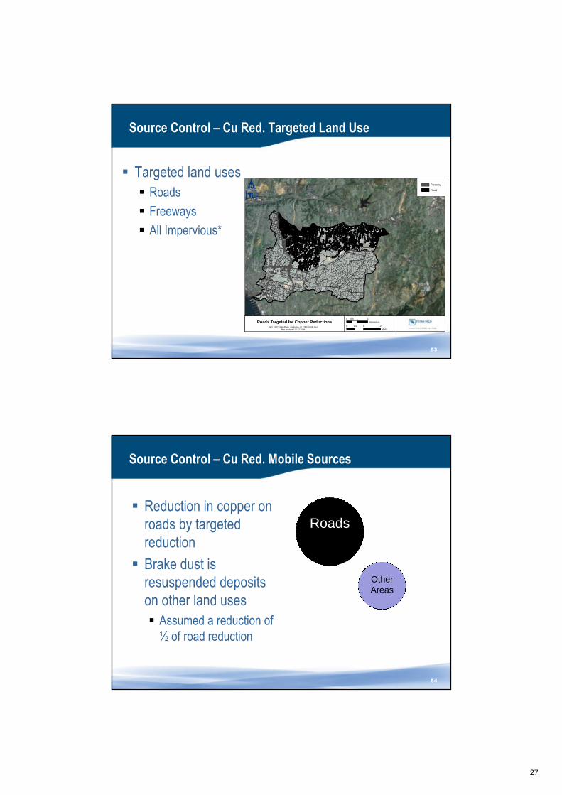
Source Control – Cu Red. Targeted Land Use
Targeted land uses
Roads
Freeways
All Impervious*
53
0 1 20.5
Kilometers
0 1 20.5
Miles
Roads Targeted for Copper ReductionsNAD_1927_StatePlane_California_VI_FIPS_0405_feet
Map produced 12-22-2009
Freeway
Road
Source Control – Cu Red. Mobile Sources
Reduction in copper onroads by targetedreduction
Brake dust isresuspended depositson other land uses
Assumed a reduction of½ of road reduction
54
Roads
OtherAreas

28
Source Control – Cu Red. Load Reductions
55
-100%
-90%
-80%
-70%
-60%
-50%
-40%
-30%
-20%
-10%
0%
19
92
19
93
19
94
19
95
19
96
19
97
19
98
19
99
20
00
20
01
20
02
20
03
20
04
20
05
Co
pp
er
Water Year
-100%
-90%
-80%
-70%
-60%
-50%
-40%
-30%
-20%
-10%
0%
Oct
ob
er
No
vem
be
r
De
cem
be
r
Jan
uar
y
Feb
ruar
y
Mar
ch
Ap
ril
May
Jun
e
July
Au
gust
Sep
tem
be
r
Co
pp
er
Modeled BMPs
Modeled BMP Scenarios and Combinations
Irrigation control ● ● ● ●Hydrologic source control
Bioretention ● ● ● ●Stormwater control
Detention basin ● ● ●Source control
Copper reduction ● ● ●Bacteria reduction ● ● ● ●Street sweeping ● ● ● ●
56

29
Source Control – Bacteria Targeted Land Use
Targeted landuses
Residential
Parks
57
Land UseAgricultureCommercialHealthCareSchoolPublicCemeteryGolfLandscapeOpenOpenRecParkMobileHomeParksMultiFamilyResidentialSingleFamilyResidentialSpacedRuralResidentialFreewayRoadMilitaryParkingIndustrialTrainTransportationWarehousingPublicStorageWater
0 1 20.5
Kilometers
0 1 20.5
Miles
Targeted Bacteria Control Land UsesNAD_1927_StatePlane_California_VI_FIPS_0405_feet
Map produced 03-18-2010
BMP Model Application
Reduce bacteria levels by 10, 20, 40 and 80%
Reduce POTFW
Reduce SQOLIM and WSQOP
58
Different BMPsimulations
BMP effectiveness
Lo
ad
red
ucti
on

30
Source Control – Bacteria Storm EMC Reductions
59
Storms ≤ 0.6 in Storms > 0.6 in
100
1,000
10,000
100,000
100 1,000 10,000 100,000
BM
PF
ec
alC
oli
form
(mg
/L)
Baseline Fecal Coliform (#/100mL)
100
1,000
10,000
100,000
100 1,000 10,000 100,000
BM
PF
ec
alC
oli
form
(mg
/L)
Baseline Fecal Coliform (#/100mL)
Modeled BMPs
Modeled BMP Scenarios and Combinations
Irrigation control ● ● ● ●Hydrologic source control
Bioretention ● ● ● ●Stormwater control
Detention basin ● ● ●Source control
Copper reduction ● ● ●Bacteria reduction ● ● ● ●Street sweeping ● ● ● ●
60

31
Street Sweeping – Swept Roads
61
Swept RoadsUnswept roads
0 1 20.5
Kilometers
0 1 20.5
Miles
Swept RoadsNAD_1927_StatePlane_California_VI_FIPS_0405_feet
Map produced 12-22-2009
Street Sweeping Effects
Reduce pollutant levelson roads
62
Str
ee
tS
weep
ing
Str
ee
tS
weep
ing
Rain
Time
Po
lluta
nt
Sto
rage

32
Street Sweeping – Load Reductions
63
-100%
-90%
-80%
-70%
-60%
-50%
-40%
-30%
-20%
-10%
0%
19
92
19
93
19
94
19
95
19
96
19
97
19
98
19
99
20
00
20
01
20
02
20
03
20
04
20
05
Vo
lum
e
Water Year
-100%
-90%
-80%
-70%
-60%
-50%
-40%
-30%
-20%
-10%
0%
19
92
19
93
19
94
19
95
19
96
19
97
19
98
19
99
20
00
20
01
20
02
20
03
20
04
20
05
Co
pp
er
Water Year-100%
-90%
-80%
-70%
-60%
-50%
-40%
-30%
-20%
-10%
0%
19
92
19
93
19
94
19
95
19
96
19
97
19
98
19
99
20
00
20
01
20
02
20
03
20
04
20
05
Feca
lCo
lifo
rm
Water Year
-100%
-90%
-80%
-70%
-60%
-50%
-40%
-30%
-20%
-10%
0%
19
92
19
93
19
94
19
95
19
96
19
97
19
98
19
99
20
00
20
01
20
02
20
03
20
04
20
05
Sed
ime
nt
Water Year
Street LoadsBacteria Load -15%Copper Load – 36%
Modeled BMPs
Modeled BMP Scenarios and Combinations
Irrigation control ● ● ● ●Hydrologic source control
Bioretention ● ● ● ●Stormwater control
Detention basin ● ● ●Source control
Copper reduction ● ● ●Bacteria reduction ● ● ● ●Street sweeping ● ● ● ●
64

33
Combination Simulations – Annual Loads
65
-100%
-90%
-80%
-70%
-60%
-50%
-40%
-30%
-20%
-10%
0%
19
92
19
93
19
94
19
95
19
96
19
97
19
98
19
99
20
00
20
01
20
02
20
03
20
04
20
05
Vo
lum
e
Water Year
-100%
-90%
-80%
-70%
-60%
-50%
-40%
-30%
-20%
-10%
0%
19
92
19
93
19
94
19
95
19
96
19
97
19
98
19
99
20
00
20
01
20
02
20
03
20
04
20
05
Co
pp
er
Water Year-100%
-90%
-80%
-70%
-60%
-50%
-40%
-30%
-20%
-10%
0%
19
92
19
93
19
94
19
95
19
96
19
97
19
98
19
99
20
00
20
01
20
02
20
03
20
04
20
05
Feca
lCo
lifo
rm
Water Year
-100%
-90%
-80%
-70%
-60%
-50%
-40%
-30%
-20%
-10%
0%
19
92
19
93
19
94
19
95
19
96
19
97
19
98
19
99
20
00
20
01
20
02
20
03
20
04
20
05
Sed
ime
nt
Water Year
Combination Simulations –Loads by Storm Size
66
0.1
1
10
100
1000
0.01 0.10 1.00 10.00
Co
pp
er
(ug
/L)
Rain (in)
100
1,000
10,000
100,000
0.01 0.10 1.00 10.00
Fe
ca
lCo
lifo
rm(#
/10
0m
L)
Rain (in)
1
10
100
1,000
10,000
0.01 0.10 1.00 10.00
TS
S(m
g/L
)
Rain (in)
0
1
10
100
1,000
10,000
0.01 0.10 1.00 10.00
Pe
ak
Flo
w(c
fs)
Rain (in)

34
BMP Scale Considerations
SiteRegional
What is SUSTAIN?
SUSTAIN – System for Urban Stormwater Treatment,and Analysis INtegratration
An ArcGIS-based framework designed to supportevaluation and decision-making:
How effective are BMPs or green infrastructure (GI) inreducing runoff and pollutant loadings?
What are the most cost-effective BMP options meeting thewater quantity and quality objectives?
• Where, what type, and how large?

35
Where It Applies?
Evaluate and select BMPs to achieve loading targets set by aTMDL
Identify protective management practices and evaluate pollutantloadings for Source Water Protection
Develop cost-effective management options for a municipal MS4program
Determine a cost-effective mix of green infrastructure measures tohelp meet optimal flow reduction goals in a CSO control study
SUSTAIN Components
Interpretation (PostProcessor)
Optimization

36
Implementation andData Collection
0%
5%
10%
15%
20%
25%
30%
35%
$0.0 $0.5 $1.0 $1.5 $2.0 $2.5 $3.0 $3.5 $4.0 $4.5
Cost ($ Million)
Eff
ective
ne
ss
(%R
ed
uctio
n)
All Solutions
Cost-Effectiveness Curve
Selected Simulation
BMP Optimization
Cost Effectiveness (CE) Curve

37
$0.0
$0.5
$1.0
$1.5
$2.0
$2.5
$3.0
$3.5
$4.0
$4.59
.9%
14
.1%
16
.6%
18
.4%
20
.3%
22
.1%
23
.4%
24
.2%
24
.8%
25
.7%
26
.6%
27
.3%
27
.9%
28
.5%
29
.6%
30
.2%
30
.6%
30
.8%
31
.1%
31
.6%
31
.8%
32
.1%
32
.4%
32
.9%
Effectiveness (% Reduction)
Co
stD
istr
ibu
tio
n($
Mill
ion
)
DRYPOND BIORETENTION
RAINBARREL POROUSPAVEMENT
Selected Simulation
55%24%
0%
21%
BMPs Selected
55%24%
0%
21%
BMP Optimization
Milwaukee Municipal Sewerage District
Proposed ultimate goal of eliminating alloverflows by 2035
Explore potential benefits of widespreadadoption of green infrastructure (GI) toreduce overflows
Potential benefits measured by: Environmental outcomes (pollution
reductions)
Economic and social outcomes (triple bottomline)
38
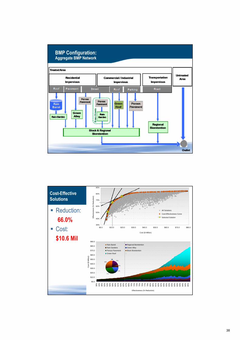
BMP Configuration:Aggregate BMP Network
$0.0
$10.0
$20.0
$30.0
$40.0
$50.0
$60.0
$70.0
$80.0
$90.0
38%
44%
48%
50%
54%
56%
58%
60%
61%
63%
65%
67%
68%
70%
72%
73%
75%
76%
77%
79%
80%
80%
81%
82%
82%
83%
83%
83%
83%
84%
84%
84%
84%
84%
85%
Effectiveness (% Reduction)
Co
st($
Mill
ion)
Rain Barrel Regional Bioretention
Rain Gardens Green Alley
Porous Pavement Block Bioretention
Green Roof
30%
40%
50%
60%
70%
80%
90%
$0.0 $10.0 $20.0 $30.0 $40.0 $50.0 $60.0 $70.0 $80.0
Cost ($ Million)
Eff
ectiv
ene
ss(%
Redu
ctio
n)
All Solutions
Cost-Effectiveness Curve
Selected Solution
Selected Solutions
1%17%
6%
17%
31%
28%
0%
Reduction:
66.0%
Cost:
$10.6 Mil
Cost-EffectiveSolutions
39
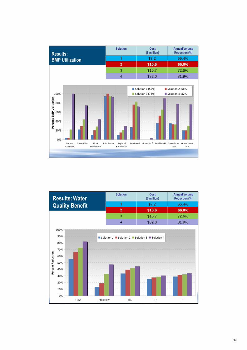
Results:BMP Utilization
Solution Cost($ million)
Annual VolumeReduction (%)
1 $7.2 55.4%
2 $10.6 66.0%
3 $15.7 72.6%
4 $32.0 81.9%
0%
20%
40%
60%
80%
100%
Porous
Pavement
Green Alley Block
Bioretention
Rain Garden Regional
Bioretention
Rain Barrel Green Roof RoadSide PP Green Street
- PP
Green Street
- BR
Pe
rce
nt
BM
PU
tili
zati
on
Solution 1 (55%) Solution 2 (66%)
Solution 3 (73%) Solution 4 (82%)
Results: WaterQuality Benefit
0%
10%
20%
30%
40%
50%
60%
70%
80%
90%
100%
Flow Peak Flow TSS TN TP
Pe
rce
nt
Re
du
ctio
n
Solution 1 Solution 2 Solution 3 Solution 4
Solution Cost($ million)
Annual VolumeReduction (%)
1 $7.2 55.4%
2 $10.6 66.0%
3 $15.7 72.6%
4 $32.0 81.9%

40
Social, economic, and environmental benefits of greeninfrastructure
Need to illustrate benefits to motivate change More beautiful neighborhoods, higher property values, improved safety
and increased jobs
Environmental stewardship benefits
Triple Bottom LineAnalysis
Job Creation
Reduced Infrastructure Cost
Reduced Pumping Costs
Increased Property Values
Improved Quality of Life andAesthetics
Increased RecreationalOpportunities
Reduced Stormwater/Sediment
Increased GroundwaterRecharge
Carbon Sequestration
Reduced Energy Use andHeat Island Effect
Develop a technical framework
for a Water Quality Funding
Initiative
Provide a tool for urban runoff
and stormwater quality
management that allows for:
BMP implementation at
local scale
Watershed management at
regional scale
LA County Department of Public Works
41
81
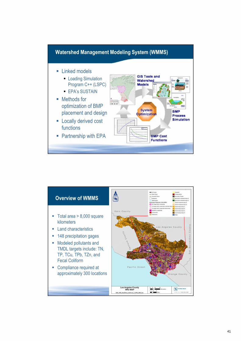
Linked models
Loading SimulationProgram C++ (LSPC)
EPA’s SUSTAIN
Methods foroptimization of BMPplacement and design
Locally derived costfunctions
Partnership with EPA
Watershed Management Modeling System (WMMS)
82
Overview of WMMS
Total area > 8,000 squarekilometers
Land characteristics
148 precipitation gages
Modeled pollutants andTMDL targets include: TN,TP, TCu, TPb, TZn, andFecal Coliform
Compliance required atapproximately 300 locations

42
Categories
Management Categories and Levels
Management Categories
Based on physiography:
• slope, impervious area, imperviousconfiguration, roads density
Factors that drive BMP selection
Management Levels
Combinations of BMPs
Increasing degree of controlsrepresented
Includes associated costs
Levels
The Watershed
D, $
D, $
D, $
ReductionOpportunity Matrix
Small-Scale Model Configuration
Treatmentpathways fromfour generalizeddrainage areas
DistributedStructural BMPs
PermeablePavement
Bioretention
Rain Barrels
43
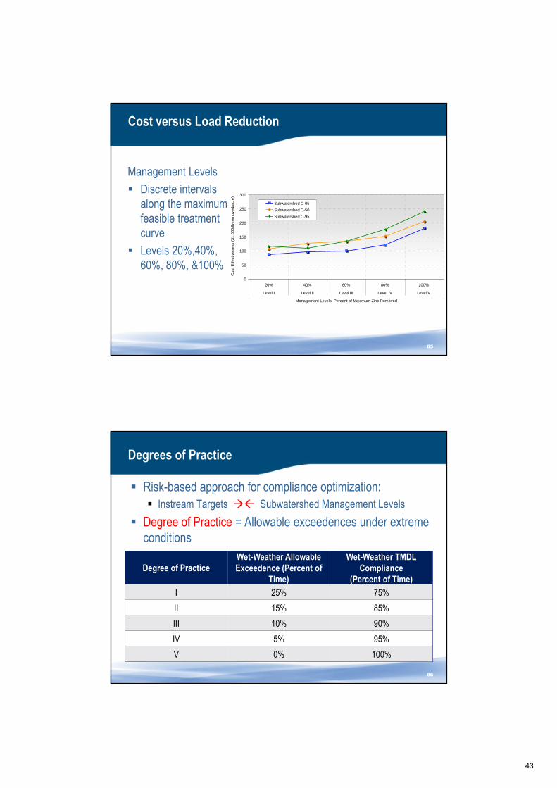
Cost versus Load Reduction
Management Levels
Discrete intervalsalong the maximumfeasible treatmentcurve
Levels 20%,40%,60%, 80%, &100%
85
0
50
100
150
200
250
300
20% 40% 60% 80% 100%
Level I Level II Level III Level IV Level V
Management Levels: Percent of Maximum Zinc Removed
Co
st
Eff
ect
ive
ne
ss($
1,0
00
/lb
-rem
ove
d/a
cre
)
Subwatershed C-05
Subwatershed C-50
Subwatershed C-95
Degrees of Practice
Risk-based approach for compliance optimization:
Instream Targets Subwatershed Management Levels
Degree of Practice = Allowable exceedences under extremeconditions
Degree of PracticeWet-Weather AllowableExceedence (Percent of
Time)
Wet-Weather TMDLCompliance
(Percent of Time)
I 25% 75%
II 15% 85%
III 10% 90%
IV 5% 95%
V 0% 100%
86

44
Management Level (V)100% Degree of Protection
100% wet-weathercompliance
Even with uniformapplication ofManagement Level V,most points do notcomply at the 100%Degree of Protection
87
Management Level (V)85% Degree of Protection
Total Treatment Cost:$44.48 billion
No Centralized BMPsRequired
For uniform applicationof Management LevelV, all points comply atthe 85% Degree ofProtection
88

45
Total Treatment Cost:$23.33 billion
Additional CentralizedBMPs for compliance:$1.09 billion
Total: $24.42 Billion
89
Management Level (IV)85% Degree of Protection
Cost Distribution vs. DoP for Proportional Scenario
90
46
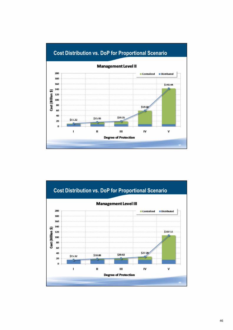
Cost Distribution vs. DoP for Proportional Scenario
91
Cost Distribution vs. DoP for Proportional Scenario
92

47
Cost Distribution vs. DoP for Proportional Scenario
93
Cost Distribution vs. DoP for Proportional Scenario
94

48
Total “Compliance” Cost by Management Level andDegree of Practice ($ Billion)
95
Total ComplianceCost ($ Billion)
96
Storm Size Analyses
• Load reduction by rainfall event
0% 0% 0% 0% 0% 0% 0% 1% 4% 1% 4% 5% 14% 7% 38% 25%0%
10%
20%
30%
40%
50%
60%
70%
80%
90%
100%
0.0
4
0.0
8
0.1
6
0.2
4
0.3
2
0.3
6
0.4
4
0.5
6
0.7
2
0.8
0.9
6
1.2
2
4.7
2
5.0
4
6.5
6
7.2
8
Precipitation Event Volume (in)
Co
pp
er
Lo
ad
Red
uc
tio
n
0%
10%
20%
30%
40%
50%
60%
70%
80%
90%
100%
Re
lati
ve
Co
ntr
ibu
tio
n(B
as
eli
ne
)
Relative Contribution Pre-Developed Reduction (45%) Reduction (55%) Reduction (65%)
49
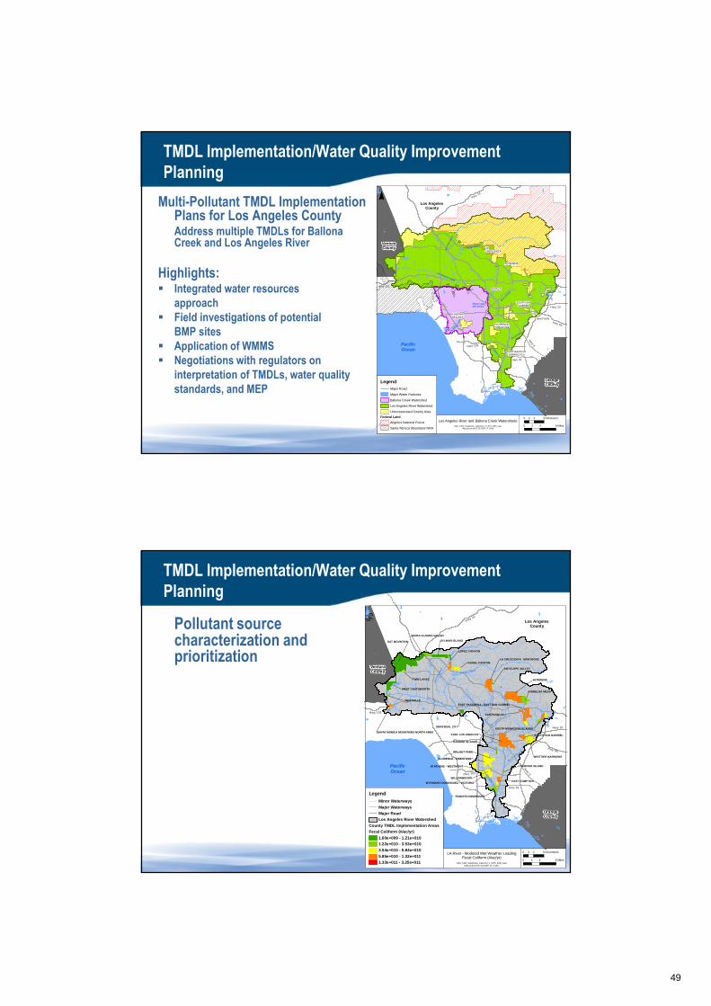
TMDL Implementation/Water Quality ImprovementPlanning
Multi-Pollutant TMDL ImplementationPlans for Los Angeles CountyAddress multiple TMDLs for BallonaCreek and Los Angeles River
Highlights: Integrated water resources
approach Field investigations of potential
BMP sites Application of WMMS Negotiations with regulators on
interpretation of TMDLs, water qualitystandards, and MEP
Los Angeles River and Ballona Creek Watersheds
NAD_1983_StatePlane_California_V_FIPS_0405_FeetMap produced 05-20-2009 - P. Cada
Hwy 10
Hwy 101
Hwy 60
LADERAHEIGHTS
FLORENCE-FIRESTONE
Tujunga Wash
Pac
oim
aW
ash
Los Angeles River
RioHondo
Ballo
na
Cre
ek
Com
pton
Cr
Seco
Arroy
o
LACRESCENTA
ALTADENA
Silver Lake(No Drain)
EAST RANCHODOMINGUEZ
SOUTH SANGABRIEL
WHITTIER
EAST LA
Hwy 14
Hwy 105
Hwy 91
Hw
y5
Legend
Major Road
Major Water Features
Ballona Creek Watershed
Los Angeles River Watershed
Unincorporated County Area
Federal Land
Angeles National Forest
Santa Monica Mountains NRA0 4 82 Miles
0 4 82 Kilometers
PacificOcean
VenturaCounty
OrangeCounty
Los AngelesCounty
TMDL Implementation/Water Quality ImprovementPlanning
Pollutant sourcecharacterization andprioritization
LA River - Modeled Wet Weather LoadingFecal Coliform (#/ac/yr)
NAD_1983_StatePlane_California_V_FIPS_0405_FeetMap produced 07-22-2009 - B. Tucker
Hwy 10
Hwy 101
Hwy 80
Tujunga Wash
Pa
c o
i ma
Was
h
Com
ptonC
r
Los Angeles River
Arroyo
Seco
RioHon
do
ALTADENA
Hwy 14
Hwy 105
Hwy 91
Hw
y5
OAT MOUNTAIN
EAST LOS ANGELES
FLORENCE - FIRESTONEWHITTIER NARROWS
LA CRESCENTA - MONTROSE
WEST CHATSWORTH
SYLMAR ISLAND
KINNELOA MESA
RANCHO DOMINGUEZ
SANTA CLARITA VALLEY
KAGEL CANYON
WALNUT PARK
W ATHENS - WESTMONT
LOPEZ CANYON
SOUTH SAN GABRIEL
W RANCHO DOMINGUEZ - VICTORIA
UNIVERSAL CITY
WESTHILLS
SAN PASQUAL
SOUTH MONROVIA ISLANDS
SANTA MONICA MOUNTAINS NORTH AREA
EAST PASADENA - EAST SAN GABRIEL
WILLOWBROOK
LYNWOOD ISLAND
TWIN LAKES
BANDINI ISLANDS
ANTELOPE VALLEY
EAST COMPTON
Legend
Minor Waterways
Major Waterways
Major Road
Los Angeles River Watershed
County TMDL Implementation Areas
Fecal Coliform (#/ac/yr)
1.60e+009 - 1.21e+010
1.22e+010 - 3.53e+010
3.54e+010 - 5.84e+010
5.85e+010 - 1.32e+011
1.33e+011 - 3.25e+0110 4 82 Miles
0 4 82 Kilometers
PacificOcean
VenturaCounty
OrangeCounty
% Los AngelesCounty

50
BMP Development and Engineering Services
Evaluating feasibilityof sites for BMPs
GIS screening
Comparison to prioritypollutant source areas
Field investigations
BMP Development and Engineering Services
Conceptual design
Understanding of thedrainage area
Flow
Pollutant loading
Opportunity for integration ofmultiple benefits
Linkage to existing stormdrain system
LOS ANGELES
COUNTY
LYNWOOD
SOUTH GATE
COUNTY
HUNTINGTON PARK
COUNTY
COUNTY
COMPTON
BELL
VERNON
COMPTON
VERNON
COUNTY
CUDAHY
COUNTY
I105
NAD_1983_StatePlane_California_V_FIPS_0405_FeetMap produced 11-17-2009 - E. Moreno
Legend
Freeways
City Boundaries
BMP Site
BMP Watershed
0 0.5 10.25Miles
0 10.5Kilometers
Mona ParkPotential Centralized BMP & Watershed Area
(FLORENCE-FIRESTONE)
(WILLOWBROOK)
(WALNUT PARK)

51
Los Angeles County TMDL Implementation Plans
Assessment of existing stormwater program elements andprocedures
A: 7.5%
B: 17.2%
C: 18.6%
D: 30.0%
E: 50.0%
F: 70.0%
G: $761.7 Mil
0%
10%
20%
30%
40%
50%
60%
70%
80%
$0 $500 $1,000 $1,500 $2,000 $2,500 $3,000 $3,500
Cost above Baseline Non-structural BMPs ($ Million)
Pe
rce
ntR
ed
uctio
n(C
op
pe
rL
oa
d)
Copper TMDL Target
Scenario 1
Scenario 2
Scenario 3
Selected Points of Interest
Alternative TMDL Solutions
TMDL Implementation/Water Quality ImprovementPlanning

52
TMDL Implementation/Water Quality ImprovementPlanning
• Conceptual designs• Quantified benefits• Considerations for
implementation• Infiltration• O&M
• Costs
Questions