applied linear algebra - unipd.itpicci/files/teaching/applied lin algebra/dispense... · 1 linear...
TRANSCRIPT
APPLIED LINEAR ALGEBRA
Giorgio Picci
November 24, 2015
1
Contents
1 LINEAR VECTOR SPACES AND LINEAR MAPS 10
1.1 Linear Maps and Matrices . . . . . . . . . . . . . . . . . . . . . . . . . . . 11
1.2 Inverse of a Linear Map . . . . . . . . . . . . . . . . . . . . . . . . . . . . 12
1.3 Inner products and norms . . . . . . . . . . . . . . . . . . . . . . . . . . . 13
1.4 Inner products in coordinate spaces (1) . . . . . . . . . . . . . . . . . . . . 14
1.5 Inner products in coordinate spaces (2) . . . . . . . . . . . . . . . . . . . . 15
1.6 Adjoints. . . . . . . . . . . . . . . . . . . . . . . . . . . . . . . . . . . . . 16
1.7 Subspaces . . . . . . . . . . . . . . . . . . . . . . . . . . . . . . . . . . . 18
1.8 Image and kernel of a linear map . . . . . . . . . . . . . . . . . . . . . . . 19
1.9 Invariant subspaces in Rn . . . . . . . . . . . . . . . . . . . . . . . . . . . 22
1.10 Invariant subspaces and block-diagonalization . . . . . . . . . . . . . . . . 23
2
1.11 Eigenvalues and Eigenvectors . . . . . . . . . . . . . . . . . . . . . . . . . 24
2 SYMMETRIC MATRICES 25
2.1 Generalizations: Normal, Hermitian and Unitary matrices . . . . . . . . . . 26
2.2 Change of Basis . . . . . . . . . . . . . . . . . . . . . . . . . . . . . . . . 27
2.3 Similarity . . . . . . . . . . . . . . . . . . . . . . . . . . . . . . . . . . . . 29
2.4 Similarity again . . . . . . . . . . . . . . . . . . . . . . . . . . . . . . . . 30
2.5 Problems . . . . . . . . . . . . . . . . . . . . . . . . . . . . . . . . . . . . 31
2.6 Skew-Hermitian matrices (1) . . . . . . . . . . . . . . . . . . . . . . . . . 32
2.7 Skew-Symmetric matrices (2) . . . . . . . . . . . . . . . . . . . . . . . . . 33
2.8 Square roots of positive semidefinite matrices . . . . . . . . . . . . . . . . . 36
2.9 Projections in Rn . . . . . . . . . . . . . . . . . . . . . . . . . . . . . . . 38
2.10 Projections on general inner product spaces . . . . . . . . . . . . . . . . . . 40
3
2.11 Gramians. . . . . . . . . . . . . . . . . . . . . . . . . . . . . . . . . . . . 41
2.12 Example: Polynomial vector spaces . . . . . . . . . . . . . . . . . . . . . . 42
3 LINEAR LEAST SQUARES PROBLEMS 43
3.1 Weighted Least Squares . . . . . . . . . . . . . . . . . . . . . . . . . . . . 44
3.2 Solution by the Orthogonality Principle . . . . . . . . . . . . . . . . . . . 46
3.3 Matrix least-Squares Problems . . . . . . . . . . . . . . . . . . . . . . . . 48
3.4 A problem from subspace identification . . . . . . . . . . . . . . . . . . . . 50
3.5 Relation with Left- and Right- Inverses . . . . . . . . . . . . . . . . . . . . 51
3.6 The Pseudoinverse . . . . . . . . . . . . . . . . . . . . . . . . . . . . . . . 54
3.7 The Euclidean pseudoinverse . . . . . . . . . . . . . . . . . . . . . . . . . 63
3.8 The Pseudoinverse and Orthogonal Projections . . . . . . . . . . . . . . . . 64
3.9 Linear equations . . . . . . . . . . . . . . . . . . . . . . . . . . . . . . . . 66
4
3.10 Unfeasible linear equations and Least Squares . . . . . . . . . . . . . . . . 68
3.11 The Singular value decomposition (SVD) . . . . . . . . . . . . . . . . . . . 70
3.12 Useful Features of the SVD . . . . . . . . . . . . . . . . . . . . . . . . . . 72
3.13 Matrix Norms . . . . . . . . . . . . . . . . . . . . . . . . . . . . . . . . . 73
3.14 Generalization of the SVD . . . . . . . . . . . . . . . . . . . . . . . . . . 75
3.15 SVD and the Pseudoinverse . . . . . . . . . . . . . . . . . . . . . . . . . . 79
4 NUMERICAL ASPECTS OF L-S PROBLEMS 81
4.1 Numerical Conditioning and the Condition Number . . . . . . . . . . . . . 86
4.2 Conditioning of the Least Squares Problem . . . . . . . . . . . . . . . . . . 90
4.3 The QR Factorization . . . . . . . . . . . . . . . . . . . . . . . . . . . . . 91
4.4 The role of orthogonality . . . . . . . . . . . . . . . . . . . . . . . . . . . 97
4.5 Fourier series and least squares . . . . . . . . . . . . . . . . . . . . 100
5
4.6 SVD and least squares . . . . . . . . . . . . . . . . . . . . . . . . . . . . . 101
5 INTRODUCTION TO INVERSE PROBLEMS 102
5.1 Ill-posed problems . . . . . . . . . . . . . . . . . . . . . . . . . . . . . . . 103
5.2 From ill-posed to ill-conditioned . . . . . . . . . . . . . . . . . . . . . . . . 104
5.3 Regularized Least Squares problems . . . . . . . . . . . . . . . . . 105
6 Vector spaces of second order random variables (1) 106
6.1 Vector spaces of second order random variables (2) . . . . . . . . . . . . . . 107
6.2 About “random vectors” . . . . . . . . . . . . . . . . . . . . . . . . . . . . 108
6.3 Sequences of second order random variables . . . . . . . . . . . . . . . . . 109
6.4 Principal Components Analysis (PCA) . . . . . . . . . . . . . . . . . . . . 111
6.5 Bayesian Least Squares Estimation . . . . . . . . . . . . . . . . . . . . . . 114
6.6 The Orthogonal Projection Lemma . . . . . . . . . . . . . . . . . . . . . . 115
6
6.7 Block-diagonalization of Symmetric Positive Definite matrices . . . . . . . . 119
6.8 The Matrix Inversion Lemma (ABCD Lemma) . . . . . . . . . . . . . . . . 122
6.9 Change of basis . . . . . . . . . . . . . . . . . . . . . . . . . . . . . . . . 123
6.10 Cholesky Factorization . . . . . . . . . . . . . . . . . . . . . . . . . . . . . 124
6.11 Bayesian estimation for a linear model . . . . . . . . . . . . . . . . 126
6.12 Use of the Matrix Inversion Lemma . . . . . . . . . . . . . . . . . 127
6.13 Interpretation as a regularized least squares . . . . . . . . . . . . . . . . . . 128
6.14 Application to Canonical Correlation Analysis (CCA) . . . . . . . . . . . . 129
6.15 Computing the CCA in coordinates . . . . . . . . . . . . . . . . . . . . . . 134
7 KRONECKER PRODUCTS 135
7.1 Eigenvalues . . . . . . . . . . . . . . . . . . . . . . . . . . . . . . . . . . . 137
7.2 Vectorization . . . . . . . . . . . . . . . . . . . . . . . . . . . . . . . . . . 138
7
7.3 Mixing ordinary and Kronecker products: The mixed-product property . . . 141
7.4 Lyapunov equations . . . . . . . . . . . . . . . . . . . . . . . . . . . . . . 145
7.5 Symmetry . . . . . . . . . . . . . . . . . . . . . . . . . . . . . . . . . . . 147
7.6 Sylvester equations . . . . . . . . . . . . . . . . . . . . . . . . . . . . . . . 152
7.7 General Stein equations . . . . . . . . . . . . . . . . . . . . . . . . . . . . 154
8 Circulant Matrices 158
8.1 The Symbol of a Circulant . . . . . . . . . . . . . . . . . . . . . . . 162
8.2 The finite Fourier Transform . . . . . . . . . . . . . . . . . . . . . . 163
8.3 Back to Circulant matrices . . . . . . . . . . . . . . . . . . . . . . . . . . 166
8
Notation
A>: transpose of A.
A∗: transpose conjugate of (the complex matrix) A .
σ(A): the spectrum (set of the eigenvalues) of A.
Σ(A): the set singular values of A.
A+: pseudoinverse of A.
Im (A): image of A.
ker(A): kernel of A.
A−1: inverse image with respect to A.
A−R: right-inverse of A (AA−R = I).
A−L: left-inverse of A (A−LA = I).
9
1 LINEAR VECTOR SPACES AND LINEAR MAPS
A vector space is a mathematical structure formed by a collection of elements called vectors,
which may be added together and multiplied by numbers, called scalars. Scalars may be
real or complex numbers, or generally elements of any field F . Accordingly the vector space
is called real- or complex- or an F− vector space. The operations of vector addition and
multiplication by a scalar must satisfy certain natural axioms which we shall not need to
report here.
The modern definition of vector space was introduced by Giuseppe Peano in 1888.
Examples of (real) vector spaces are the arrows in a fixed plane or in the three-dimensional
space representing forces or velocity in Physics. Vectors may however be very general objects
such as functions or polynomials etc. provided they can be added together and multiplied
by scalars to give elements of the same kind.
The vector space composed of all the n-tuples of real or complex numbers is known as a
coordinate space and is usually denoted by Rn or Cn.
10
1.1 Linear Maps and Matrices
The concepts of linear independence, basis, coordinates, etc. are given for granted. Vector
spaces admitting a basis consisting of a finite number n of elements are called n−dimensional
vector spaces. Example: the complex numbers C are a two-dimensional real vector space,
with a two dimensional basis consisting of 1 and the imaginary unit i.
A function between two vector spaces f : V → W is a linear map if for all scalars α, β
and all vectors v1, v2 in V
f (αv1 + βv2) = αf (v1) + βf (v2)
When V and W are finite dimensional, say n- and m- dimensional, a linear map can be
represented by a m × n matrix with elements in the field of scalars. The matrix acts by
multiplication on the coordinates of the vectors of V , written as n × 1 matrices (which
are called column vectors) and provides the coordinates of the image vectors in W . The
matrix hence depends on the choice of basis in the two vector spaces.
The set of all n × m matrices with elements in R (resp. C) form a real (resp. complex)
vector space of dimension mn. These vector spaces are denoted Rn×m or Cn×m respectively.
11
1.2 Inverse of a Linear Map
Let V and W be finite dimensional, say n- and m- dimensional. By choosing bases in the
two spaces any linear map f : V → W is represented by a matrix A ∈ Cm×n.
Proposition 1.1 If f : V → W is invertible the matrix A must also be invertible and
the two vector spaces must have the same dimension (say n).
Invertible matrices are also called non-singular. The inverse A−1 can be computed by the
so-called Cramer rule
A−1 =1
detAAdj(A)
where he “algebraic adjoint ” Adj(A) is the transpose of a matrix having in position (i, j)
the determinant of the complement to row i and column j (an n − 1 × n − 1 matrix)
multiplied by the factor (−1)i+j.
This rule is seldom used for actual computations. There is a wealth of algorithms to compute
inverses which apply to matrices of specific structure. In fact computing inverses is seldom
of interest per se; one may rather have to look for algorithms which compute solutions of a
linear system of equations Ax = b.
12
1.3 Inner products and norms
An inner product on V is a map 〈·, ·〉 : V × V → C satisfying the following require-
ments.
• Conjugate symmetry:
〈x, y〉 = 〈y, x〉
• Linearity in the first argument:
〈ax, y〉 = a〈x, y〉〈x + y, z〉 = 〈x, z〉 + 〈y, z〉
• Positive-definiteness:
〈x, x〉 ≥ 0 , 〈x, x〉 = 0⇒ x = 0
The norm induced by a inner product is ‖x‖ = +√〈x, x〉.
This is the “length” of the vector x. Directly from the axioms, one can prove the Cauchy-
Schwarz inequality: for x, y elements of V
|〈x, y〉| ≤ ‖x‖ · ‖y‖
with equality if and only if x and y are linearly dependent. This is one of the most important
inequalities in mathematics. It is also known in the Russian literature as the CauchyBun-
yakovskySchwarz inequality.
13
1.4 Inner products in coordinate spaces (1)
In the vector space Rn (in Cn you must use conjugation), the bilinear function:
〈·, ·〉 : Rn × Rn −→ R, 〈u, v〉 := u>v Column vectors
has all the prescribed properties to be an inner product. It induces the Euclidean norm
on Rn:
‖ · ‖ : Rn −→ R+ , ‖u‖ :=√u>u
The bilinear form defined on Cn×m × Cn×m by
〈A, B〉 : (A, B) 7→ tr (AB>) = tr (B>A) (1.1)
where tr denotes trace and B is the complex conjugate of B, is a bona fide inner product
on Cn×m. The matrix norm defined by the inner product (1.1),
‖A‖F := 〈A, A〉1/2 = [tr AA>]1/2 (1.2)
is called the Frobenius, or the weak norm of A.
14
1.5 Inner products in coordinate spaces (2)
More general inner products in Cn can be defined as follows.
Definition 1.1 A square matrix A ∈ Cn×n is Hermitian if
A> = A
and positive semidefinite if x>Ax ≥ 0 for all x ∈ Cn. The matrix is called positive
definite if x>Ax can be zero only when x = 0.
There are well-known tests of positive definiteness based on checking the signs of the prin-
cipal minors which should all be positive.
Given an Hermitian positive definite matrix Q we define the weighted inner product 〈·, ·〉Qin the coordinate space Cn by setting
〈x, y〉Q : = x>Qy
This clearly satisfies the axioms of inner product.
Problem 1.1 Show that any inner product in Cn must have this structure for a suit-
able Q. Is Q uniquely defined ?
15
1.6 Adjoints.
Consider a linear map A : X → Y , both finite-dimensional vector spaces endowed with
inner products 〈·, ·〉X and 〈·, ·〉Y respectively.
Definition 1.2 The adjoint, of A : X → Y is a linear map A∗ : Y → X , defined
by the relation
〈y, Ax〉Y = 〈A∗y, x〉X , x ∈X , y ∈ Y (1.3)
Problem 1.2 Prove that A∗ is well-defined by the condition (1.3).
Hint: here you must use the fact that X and Y are finite-dimensional.
Example: Let A : Cn → Cm where the spaces are equipped with weighted inner products,
say
〈x1, x2〉|Cn = x>1 Q1x2, 〈y1, y2〉|Cm = y>1 Q2y2
where Q1, Q2 are Hermitian positive definite matrices. Then we have
16
Proposition 1.2 The adjoint of the linear map A : X → Y defined by a matrix
A : Cn → Cm with weighted inner products as above, is
A∗ = Q−11 A>Q2 (1.4)
where A> is the conjugate transpose of A.
Problem 1.3 Prove proposition 1.2.
Let A : Cn → Cm and assume that Q1 and Q2 = I are both identity matrices. Both inner
products in this case are Euclidean inner products. Then
A∗ = A>
i.e. the adjoint is the Hermitian conjugate. In particular, for a real matrix the adjoint is
just the transpose. For any square Hermitian matrix the adjoint coincides with the original
matrix. The linear map defined by the matrix is then called a self-adjoint operator. In the
real case self-adjoint operators are represented by symmetric matrices. Note that all this is
true only if the inner products are Euclidean.
17
1.7 Subspaces
A subset of a vector space X ⊂ V which is itself a vector space with the same field of
scalars is called a subspace. Subspaces of finite-dimensional vector spaces are automatically
closed with respect to any inner product induced norm topology. This is not necessarily so
if V is infinite dimensional.
Definition 1.3 Let X , Y ⊂ V be subspaces. Then
1. X ∨ Y := v ∈ V : v = x + y, x ∈ X , y ∈ Y is called the vector sum of X
and Y .
2. When X ∩ Y = 0 the vector sum is called direct. Notation: X + Y .
3. When X + Y = V the subspace Y is called a Direct Complement of X in V .
Notation: Often in the literature vector sum is denoted by a + and direct vector sum by
a ⊕. We shall use the latter symbol for orthogonal direct sum.
Let Rn = X +Y with dimX = k and dimY = m. Then n = k+m and there exist
a basis in Rn such that
v ∈X ⇐⇒ v =
[x
0
], x ∈ Rk , 0 ∈ Rm, v ∈ Y ⇐⇒ v =
[0
y
], 0 ∈ Rk , y ∈ Rm
18
1.8 Image and kernel of a linear map
Definition 1.4 Let A ∈ Rn×m.
1. Im (A) := v ∈ Rn : v = Aw, w ∈ Rm (subspace of Rn).
2. ker(A) := v ∈ Rm : Av = 0 (subspace of Rm).
Definition 1.5 Let V subspace of Rn. The orthogonal complement of V is defined as
V ⊥ := w ∈ Rn : 〈w, v〉 = 0 ∀v ∈ V = w ∈ Rn : 〈v, w〉 = 0 ∀v ∈ V
Matlab
orth: “Q = orth(A)” computes a matrix Q whose columns are an orthonormal basis for
Im (A) (i.e. Q>Q = I , Im (Q) = Im (A) and the number of columns of Q is the rank(A)).
null: “Z = null(A)” computes a matrix Z whose columns are an orthonormal basis for
ker(A).
19

Proposition 1.3 Let A ∈ Rn×m,
1. ker(A) = ker(A>A).
2. ker(A) = [Im (A>)]⊥ that is Rn = ker(A)⊕ Im (A>) .
3. Im (A) = [ker(A>)]⊥ that is Rn = Im (A)⊕ ker(A>).
4. Im (A) = Im (AA>).
Proof.
1. Let v ∈ ker(A) ⇒ Av = 0 ⇒ A>Av = 0 ⇒ v ∈ ker(A>A).
Let v ∈ ker(A>A)⇒ A>Av = 0⇒ v>A>Av = 0⇒ ‖Av‖2 = 0⇒ Av = 0⇒ v ∈ ker(A).
2.
v ∈ ker(A) ⇐⇒Av = 0 ⇐⇒v>A> = 0 ⇐⇒v>A>w = 0 ∀ w ∈ Rn ⇐⇒v ∈ [Im (A>)]⊥
3. Immediate consequence of 2.
4. Immediate consequence of 1. and 2.
Hence:
if V = Im (A) then V ⊥ = Im (B) where B can be computed in Matlab as B = null(A>).
20
Intersecting kernels is easy:
ker(A) ∩ ker(B) = ker
([A
B
]).
Similarly, adding images is easy:
Im (A) ∨ Im (B) = Im ([A | B])
Adding kernels can now be done by using the image representation.
For example: ker(A) ∨ ker(B) can be computed by representing ker(A) as Im (A1) and
ker(B) as Im (B1) (Matlab function “null”). Intersection of images can be done as
Im (A) ∩ Im (B) = [ker(A>)]⊥ ∩ [ker(B>)]⊥ = [ker(A>) ∨ ker(B>)]⊥.
Problem 1.4 State and prove Proposition 1.3 for complex matrixes.
21
1.9 Invariant subspaces in Rn
Let A ∈ Rn×m and V be a subspace of Rm. We denote by AV the image of V through
the map A.
If V = Im (V ), then AV = Im (AV ).
Definition 1.6 Let A ∈ Rn×n and let V be a subspace of Rn. We say that V is
invariant for A or A-invariant if AV ⊆ V (i.e. ∀x ∈ V , Ax ∈ V ).
If in addition, V ⊥ is also invariant, we say that V is a reducing subspace.
It is trivial that both Im (A) and ker(A) are A-invariant.
Let V be a matrix whose columns form a basis for V . Then V is A-invariant if and only
if Im (AV ) ⊆ Im (V ).
Problem 1.5 Let A ∈ Rn×n and V be a subspace of Rn. Prove that:
1. If A is invertible, V is A-invariant if and only if it is A−1-invariant.
2. V is A-invariant if and only if V ⊥ is A>-invariant.
3. If V is invariant and A is symmetric; i.e. A = A> then V is a reducing subspace.
22
1.10 Invariant subspaces and block-diagonalization
Let A ∈ Rn×n and Rn = V + W where V is A-invariant. Then there is a choice of basis
in Rn with respect to which A has the representation
A =
[A1 A1,2
0 A2
]where A1 ∈ Rk×k with k = dim V . In any such a basis vectors in V are represented as
columns
[v
0
]with the last n− k components equal to zero.
If both V and W are invariant then there is basis in Rn with respect to which A has a
block-diagonal representation
A =
[A1 0
0 A2
].
The key to finding invariant subspaces is spectral analysis.
23
1.11 Eigenvalues and Eigenvectors
Along some directions a square matrix A ∈ Rn×n acts like a multiplication by a scalar
Av = λv
the scalar factor λ is called eigenvalue associated to the eigenvector v. Eigenvectors are
actually directions in space and are usually normalized to unit norm. In general eigenvalues
(and eigenvectors) are complex as they must be roots of the characteristic polynomial
equation
χA(λ) := det(A− λI) = 0
which is of degree n in λ and hence has n (not necessarily distinct) complex roots λ1, . . . , λn.This set is called the spectrum of A and is denoted σ(A). The multiplicity of λk as a root
of the characteristic polynomial is called the algebraic multiplicity.
When eigenvectors are linearly independent they form a basis in which the matrix A looks
like multiplication by a diagonal matrix whose elements are the eigenvalues. Unfortunately
this happens only for special classes of matrices.
24
2 SYMMETRIC MATRICES
Proposition 2.1 Let A = A> ∈ Rn. Then
1. The eigenvalues of A are real and the eigenvectors can be chosen to be a real
orthonormal basis.
2. A is diagonalizable by an orthogonal transformation (∃T s.t. T>T = I and T>AT
diagonal).
Proof. (sketch)
1. Let λ be an eigenvalue and v a corresponding eigenvector,
λv∗v = v∗Av = (Av)∗v = λv∗v ⇒ λ = λ. Therefore solutions of the real equation
(A− λI)v = 0 can be chosen to be real.
2. If v1 and v2 are eigenvectors corresponding to λ1 6= λ2
then v>1 Av2 = λ1v>1 v2 = λ2v
>1 v2 ⇒ v>1 v2 = 0. Hence ker(A − λiI) ⊥ ker(A − λjI)
whenever i 6= j.
3. ker(A − λkI) is A-invariant; in fact reducing. Hence A restricted to this subspace is
represented by a nk×nk matrix having as only eigenvalue λk and characteristic polynomial
(λ − λk)rk where rk is the algebraic multiplicity of λk. But then dimension and degree of
the characteristic polynomial must coincide. Therefore nk = rk.
4. Hence we can take a basis of rk orthonormal eigenvectors corresponding to each distinct
λk. Then A is diagonalizable by an orthonormal choice of basis.
25
2.1 Generalizations: Normal, Hermitian and Unitary matrices
Definition 2.1 A matrix A ∈ Cn×n is :
1. Hermitian if A = A∗ where A∗ = A> and skew-Hermitian if A∗ = −A.
2. Unitary if AA∗ = A∗A = I
3. Normal if AA∗ = A∗A.
Real unitary matrices are called orthogonal. Both have orthonormal columns with
respect to the proper inner product.
Clearly, Hermitian, skew-Hermitian and unitary matrices are all Normal. It can be shown
that all Normal matrices are diagonalizable. In particular,
Proposition 2.2 Let A ∈ Cn×n be Hermitian. Then
1. The eigenvalues of A are real and the eigenvectors can be chosen to be an orthonor-
mal basis in Cn.
2. A is diagonalizable by a unitary transformation: i.e. there exist T ∈ Cn×n with
T ∗T = TT ∗ = I such that T ∗AT is diagonal.
Problem 2.1 Prove that all eigenvalues of a Hermitian positive semidefinite matrix
are nonnegative.
26
2.2 Change of Basis
Let V be a finite dimensional vector space with basis u1, . . . , un and A : V → V be a linear
map represented in the given basis by the n× n matrix A.
Let u1, . . . , un be another basis in V.
Problem 2.2 How does the matrix A change under the change of basis u1, . . . , un ⇒u1, . . . , un ?
Answer:
Theorem 2.1 Let T be the matrix of coordinate vectors with the k-th column repre-
senting uk in terms of the old basis u1, . . . , un. Then the matrix representation of A
with respect to the new basis is
A = T−1AT .
Proof: using matrix notation
uk =∑j
tj,kuj ⇒[u1 . . . un
]=[u1 . . . un
]T (2.5)
27
Clearly T must be invertible (show this by contradiction). Then write
Auk :=∑j
Aj,kuk; k = 1, . . . , n
as a row matrix [Au1 . . . Aun
]=[u1 . . . un
]A =
[u1 . . . un
]TA
Take any vector x ∈ V having coordinate vector ξ ∈ Cn with respect to the new basis and
ξ with respect to the old basis and let η = Aξ and η := Aξ so that[u1 . . . un
]η =
[u1 . . . un
]Aξ =
[u1 . . . un
]TAξ
but in the old basis the left member[u1 . . . un
]η is[u1 . . . un
]Aξ so that by uniqueness
of the coordinates Aξ = TAξ and since from (2.5) it follows that ξ = T−1ξ we have the
assertion.
28
2.3 Similarity
Definition 2.2 Matrices A and B in ∈ Cn×n are similar if there is a nonsingular
T ∈ Cn×n such that B = T−1AT .
Problem 2.3 Show that similar matrices have the same eigenvalues (easy!).
The following is a classical problem in Linear Algebra
Problem 2.4 Show that a matrix is similar to its own transpose; i.e. there is a
nonsingular T ∈ Rn×n such that A> = T−1AT .
Hence A and A> must have the same eigenvalues. Solving this problem requires the use of
the Jordan Form which we shall not dig into. But you may easily prove that
Proposition 2.3 A Jordan block matrix
J(λ) :=
λ 0 . . . . . . 0
1 λ 0 . . . 0... ...
0 . . . . . . 1 λ
is similar to its transpose.
29
2.4 Similarity again
The following is the motivation for introducing the Jordan Form of a matrix.
Problem 2.5 Find necessary and sufficient conditions for two matrices of the same
dimension to be similar.
Having the same eigenvalues is just a necessary conditions. For example you may check
that the two matrices
J1(λ) :=
[λ 0
1 λ
], J2(λ) :=
[λ 0
0 λ
]have the same eigenvalue(s) but are not similar. The Jordan Canonical Form of a
matrix A is just a block diagonal matrix made of square Jordan blocks like J(λk) (not
necessarily distinct), of dimension n ≥ 1, where the λk are all the (distinct) eigenvalues of
A.
30
Some Jordan blocks may actually be of dimension 1×1. So the Jordan Canonical Form may
show a diagonal submatrix. For example the identity matrix is already in Jordan Canonical
Form.
The Jordan form is unique modulo permutation of the sub-blocks.
Theorem 2.2 Two matrices of the same dimension are similar if and only if have
the same Jordan Canonica Form.
2.5 Problems
1. Describe the Jordan canonical form of a symmetric matrix.
2. Show that any Jordan block J(λ) of arbitrary dimension n×n has just one eigenvector.
3. Compute the second and third power matrix of a Jordan block J(λ) of dimension 3× 3
and find the normalized eigenvectors of J(λ), J(λ)2, J(λ)3 .
31
2.6 Skew-Hermitian matrices (1)
Recall that a matrix A ∈ Cn×n is Skew-Hermitian if A∗ = −A, Skew-Symmetric if
A> = −A.
Problem 2.6 Prove that for skew-Hermitian matrices the quadratic form x∗Ax must
be identically zero. Therefore A is positive semidefinite if and only if its Hermitian
component:
AH :=1
2[A + A∗ ]
is such.
Hence there is no loss of generality to assume that a positive semidefinite matrix is Hermitian
(or symmetric in the real case).
Problem 2.7 Prove that a skew symmetric matrix of odd dimension is always singu-
lar. Is this also true for Hermitian skew symmetric matrices?
32
2.7 Skew-Symmetric matrices (2)
The eigenvalues of a skew-symmetric matrix always come in pairs ±λ (except in the odd-
dimensional case where there is an additional unpaired 0 eigenvalue).
Problem 2.8 Show that for a real skew-symmetric matrix χA>(λ) = χ−A(λ) = (−1n)χA(−λ)
Hence the nonzero eigenvalues of a real skew-symmetric matrix are all pure imagi-
nary and thus of the form iλ1,−iλ1, iλ2,−iλ2, where each of the λk is real.
Hint: The characteristic polynomial of a real skew-symmetric matrix has real coefficients.
Since the eigenvalues of a real skew-symmetric matrix are imaginary it is not possible to
diagonalize one by a real matrix. However, it is possible to bring every skew-symmetric
matrix to a block diagonal form by an orthogonal transformation.
33
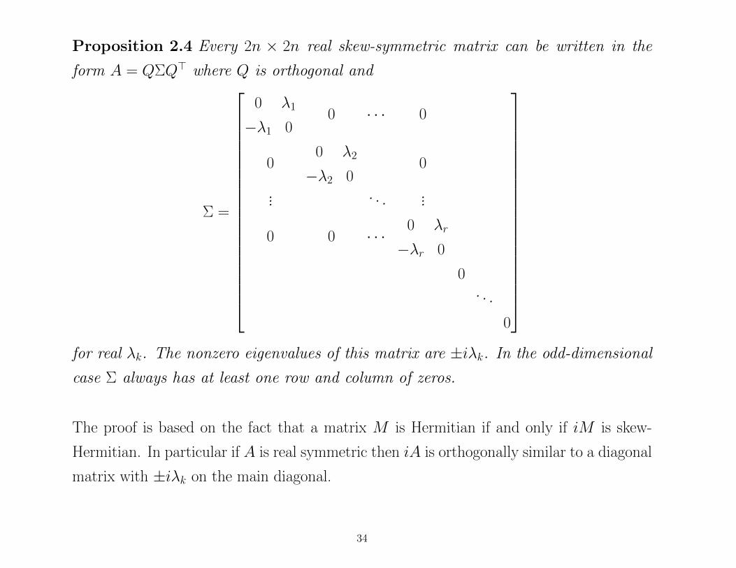
Proposition 2.4 Every 2n × 2n real skew-symmetric matrix can be written in the
form A = QΣQ> where Q is orthogonal and
Σ =
0 λ1
−λ1 00 · · · 0
00 λ2
−λ2 00
... . . . ...
0 0 · · ·0 λr
−λr 0
0. . .
0
for real λk. The nonzero eigenvalues of this matrix are ±iλk. In the odd-dimensional
case Σ always has at least one row and column of zeros.
The proof is based on the fact that a matrix M is Hermitian if and only if iM is skew-
Hermitian. In particular if A is real symmetric then iA is orthogonally similar to a diagonal
matrix with ±iλk on the main diagonal.
34
More generally, every complex skew-symmetric (i.e. skew Hermitian) matrix can be written
in the form A = UΣU ∗ where U is unitary and Σ has the block-diagonal form given above
with complex λk. This is an example of the Youla decomposition of a complex square
matrix.
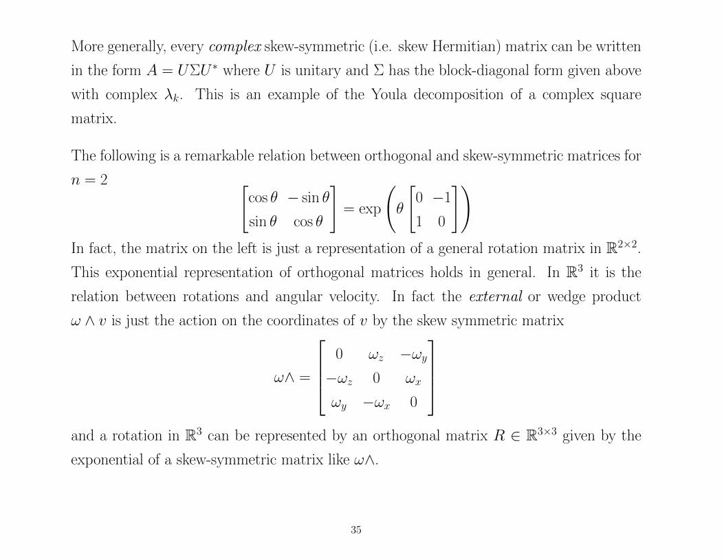
The following is a remarkable relation between orthogonal and skew-symmetric matrices for
n = 2 [cos θ − sin θ
sin θ cos θ
]= exp
(θ
[0 −1
1 0
])In fact, the matrix on the left is just a representation of a general rotation matrix in R2×2.
This exponential representation of orthogonal matrices holds in general. In R3 it is the
relation between rotations and angular velocity. In fact the external or wedge product
ω ∧ v is just the action on the coordinates of v by the skew symmetric matrix
ω∧ =
0 ωz −ωy−ωz 0 ωx
ωy −ωx 0
and a rotation in R3 can be represented by an orthogonal matrix R ∈ R3×3 given by the
exponential of a skew-symmetric matrix like ω∧.
35
2.8 Square roots of positive semidefinite matrices
Let A ∈ Rn with A = A> ≥ 0. Even if A > 0, there are many, in general rectangular,
matrices Q such that QQ> = A. Any such matrix is called a square root of A. However
there is only one symmetric square root.
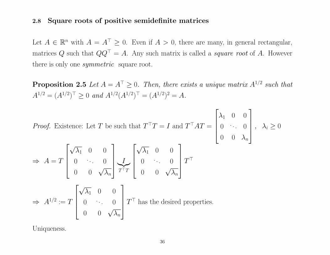
Proposition 2.5 Let A = A> ≥ 0. Then, there exists a unique matrix A1/2 such that
A1/2 = (A1/2)> ≥ 0 and A1/2(A1/2)> = (A1/2)2 = A.
Proof. Existence: Let T be such that T>T = I and T>AT =
λ1 0 0
0 . . . 0
0 0 λn
, λi ≥ 0
⇒ A = T
√λ1 0 0
0 . . . 0
0 0√λn
I︸︷︷︸T>T
√λ1 0 0
0 . . . 0
0 0√λn
T>
⇒ A1/2 := T
√λ1 0 0
0 . . . 0
0 0√λn
T> has the desired properties.
Uniqueness.
36
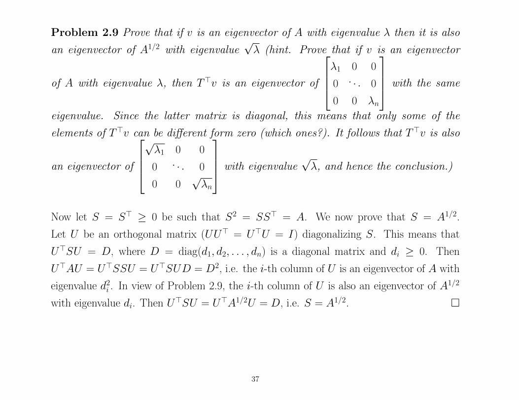
Problem 2.9 Prove that if v is an eigenvector of A with eigenvalue λ then it is also
an eigenvector of A1/2 with eigenvalue√λ (hint. Prove that if v is an eigenvector
of A with eigenvalue λ, then T>v is an eigenvector of
λ1 0 0
0 . . . 0
0 0 λn
with the same
eigenvalue. Since the latter matrix is diagonal, this means that only some of the
elements of T>v can be different form zero (which ones?). It follows that T>v is also
an eigenvector of
√λ1 0 0
0 . . . 0
0 0√λn
with eigenvalue√λ, and hence the conclusion.)
Now let S = S> ≥ 0 be such that S2 = SS> = A. We now prove that S = A1/2.
Let U be an orthogonal matrix (UU> = U>U = I) diagonalizing S. This means that
U>SU = D, where D = diag(d1, d2, . . . , dn) is a diagonal matrix and di ≥ 0. Then
U>AU = U>SSU = U>SUD = D2, i.e. the i-th column of U is an eigenvector of A with
eigenvalue d2i . In view of Problem 2.9, the i-th column of U is also an eigenvector of A1/2
with eigenvalue di. Then U>SU = U>A1/2U = D, i.e. S = A1/2.
37
2.9 Projections in Rn
Here we work on the real vector space Rn endowed with the Euclidean inner product. More
general notions of projections will be encountered later.
Definition 2.3 Let Π ∈ Rn×n. Π is a projection matrix if Π = Π2. Π is an orthogonal
projection if it is a projection and Π = Π>.
Note that Π is a (orthogonal) projection ⇔ I − Π is also an (orthogonal) projection. Let
Π be a projection and V = Im (Π). We say that Π projects onto V .
Proposition 2.6 If Π is an orthogonal projector that projects onto V ⇒ I−Π projects
onto V ⊥.
Proof. For any x, y ∈ Rn, v := Πx ⊥ w := (I − Π)y (in fact: v>w = x>Π(I − Π)y = 0.)
⇒ Im (I − Π) ⊆ V ⊥.
Conversely, let x ∈ V ⊥ ⇒ 0 = x>Πx = x>ΠΠx = x>Π>Πx = ‖Πx‖2 ⇒ Πx = 0 ⇒(I − Π)x = x ⇒ x ∈ Im (I − Π).
38
Proposition 2.7 If Π is an orthogonal projection then: σ(Π) ⊆ 0, 1; i.e. the eigen-
values are either 0 or 1. Π is in fact similar to
[I 0
0 0
]. The dimension of the identity
matrix is that of the range space.
Proof.
Π is symmetric hence diagonalizable by proposition 2.1 and since it is positive semidefinite
(as x>Πx = x>Π>Πx = ‖Πx‖2 ≥ 0) has real eigenvalues. Then v = Π2v = λv = λ2v,
v 6= 0 ⇒ λ = λ2 ⇒ λ ∈ 0, 1.
Proposition 2.8 Let Πk be orthogonal projections onto Vk = Im (Πk), k = 1, 2. Then
1. Π := Π1+Π2 is a projection⇔ V1 ⊥ V2 in which case Π projects onto the orthogonal
direct sum V1 ⊕ V2.
2. Π := Π1Π2 is a projection iff Π1Π2 = Π2Π1 in which case Π projects onto the
intersection V1 ∩ V2.
For a proof see the book of Halmos [8, pp. 44–49]. This material lies at the grounds of
spectral theory in Hilbert spaces.
39
2.10 Projections on general inner product spaces
Problem 2.10 Prove that if A a linear map in an arbitrary inner product space
(V , 〈·, ·〉) then
V = Im A ⊕ kerA∗ = kerA ⊕ Im A∗
Hence if A is self-adjoint then
V = Im A ⊕ kerA
(Hint: The proof follows from the proof of Proposition 1.3.)
Definition 2.4 In an arbitrary inner product space (V , 〈·, ·〉) an idempotent linear
map P : V → V ; i.e. such that P 2 = P , is called a projection. If P is self-adjoint; i.e.
P = P ∗ the projection is an orthogonal projection.
Hence if X is the range space of a projection, we have PX = X and if P is an orthogonal
projection, the orthogonal complement X ⊥ is the kernel; i.e. PX ⊥ = 0.
Note that all facts exposed in Section 2.9 hold true in this more general context provide
you substitute the Euclidena space Rn with (V , 〈·, ·〉) and the transpose with adjoint.
40
2.11 Gramians.
Let v1, . . . , vn be vectors in (V , 〈·, ·〉). Their Gramian is the Hermitian (in the real case
symmetric) matrix
G(v1, . . . , vn) :=
〈v1, v1〉 . . . 〈v1, vn〉. . . . . . . . .
〈vn, v1〉 . . . 〈vn, vn〉
The Gramian is always positive semidefinite. In fact, let v =
∑k xkvk ;xk ∈ C, then
‖v‖2 = x>G(v1, . . . , vn)x
where x :=[x1 . . . xn
]>. If the vk’s are linearly independent, x is the vector of coordinates
of v.
Problem 2.11 Show that G(v1, . . . , vn) is positive definite if and only if the vectors
v1, . . . , vn are linearly independent.
41
2.12 Example: Polynomial vector spaces
Let (V , 〈·, ·〉) be the vector space of real polynomials restricted to the interval [−1, 1] with
inner product
〈p, q〉 :=
∫ +1
−1
p(x)q(x) dx
This space is not finite dimensional but if we only consider polynomials of degree less or
equal to n we obtain for each n, a vector subspaces of dimension n + 1. V has a natural
basis consisting of the monomials
1, x, x2, . . .
the coordinates of a vector p(x) ∈ V with respect to this basis being just the ordinary
coefficients of the polynomial. To find an orthonormal basis we may use the classical Gram-
Schmidt sequential orthogonalization procedure (see Section 4.3). In this way we obtain
the Legendre Polynomials
P0(x) = 1 , P1(x) = x , P2(x) = 1/2(3x2 − 1) , P3(x) = 1/2(5x3 − 3x) ,
P4(x) = 1/8(35x4 − 30x2 + 3) , P5(x) = 1/8(63x5 − 70x3 + 15x) ,
P6(x) = 1/(16)(231x6 − 315x4 + 105x2 − 5). , etc.
There are books written about polynomial vector spaces, see [4].
42
3 LINEAR LEAST SQUARES PROBLEMS
Problem 3.1 Fit, in some “reasonable ” way, a parametric model of known structure
to measured data.
Given: measured output data (y1, . . . , yN), assumed real-valued for now, and “input” (or
exogenous) variables (u1, . . . , uN), in N experiments, plus a candidate class of parametric
models (from a priori information)
yt(θ) = f (ut, θ, t) t = 1, . . . , N , θ ∈ Θ ⊆ Rp
Use a quadratic approximation criterion
V (θ) :=
N∑1
[yt − yt(θ)]2 =
N∑1
[yt − f (ut, θ, t)]2
The “best” model corresponds to the value(s) θ, of θ minimizing V (θ)
V (θ) = minθ∈Θ
V (θ) .
This is a simple empirical rule for constructing models from measured data. May come out
from statistical estimation criteria in problems with probabilistic side information.
Obviously θ depends on (y1, . . . , yN) (u1, . . . , uN);
θ = θ(y1, . . . , yN ; u1, . . . , uN) ,
is called a Least-Squares-Estimator of θ. No statistical significance attached to this word.
43
3.1 Weighted Least Squares
Reasonable to weight the modeling errors by some positive coefficients qt corresponding to
more or less reliable results of the experiment. This leads to Weighted Least Squares,
criteria of the type
VQ(θ) :=
N∑1
qt [y(t)− f (ut, θ, t)]2 ,
where q1, . . . , qN are positive numbers, which are large for reliable data and small for bad
data. In general may introduce a symmetric positive-definite weight matrix Q
VQ(θ) = [y − f (u, θ)]> Q [y − f (u, θ)] = ‖y − f (u, θ)‖2Q ,
where
y =
y1
...
yN
f (u, θ) =
f (u1, θ, 1)...
f (uN , θ, N)
(3.6)
The minimization of VQ(θ) can be done analytically when the model is linear in the
parameters, that is
f (ut, θ, t) =
p∑1
si(ut, t) θi , t = 1, . . . , N .
44
Since ut is a known quantity can rewrite this as
f (ut, θ, t) := s>(t) θ ,
with s>(t) a p-dimensional row vector which is a known function of u and of the index t.
Using vector notations, introducing the N × p , Signal matrix,
S =
s>(1)
...
s>(N)
.
we get the linear model class yθ = Sθ , θ ∈ Θ and the problem becomes to minimize
with respect to θ the quadratic form
VQ(θ) = [y − Sθ]> Q[y − Sθ] = ‖y − Sθ‖2Q . (3.7)
The minimization can be done by elementary calculus. However it is more instructive to do
this by geometric means using the Orthogonal Projection Lemma.
Make RN into an inner product space by introducing the inner product 〈x, y〉Q = x>Qy
and let the corresponding norm be denoted by ‖ · ‖Q. Let S be the linear subspace of RN
spanned by the columns of the matrix S. Then the minimization of ‖y − Sθ‖2Q is just the
minimum distance problem of finding the vector y ∈ S of shortest distance from the data
vector y. See the picture below.
45
3.2 Solution by the Orthogonality Principle
y
S
PPPPPPPq
Sθ
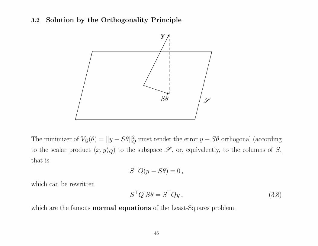
The minimizer of VQ(θ) = ‖y − Sθ‖2Q must render the error y − Sθ orthogonal (according
to the scalar product 〈x, y〉Q) to the subspace S , or, equivalently, to the columns of S,
that is
S>Q(y − Sθ) = 0 ,
which can be rewritten
S>Q Sθ = S>Qy . (3.8)
which are the famous normal equations of the Least-Squares problem.
46
Let us first assume that
rank S = p ≤ N . (3.9)
This is an identifiability condition of the model class. Each model corresponds 1 : 1 to
a unique value of the parameter. Under this condition the equation (3.8) has a unique
solution which we denote θ(y) given by
θ(y) = [S>QS ]−1 S>Qy , (3.10)
which is a linear function of the observations y. For short we shall denote θ(y) = Ay. Then
Sθ(y) := SAy is the orthogonal projection of y onto the subspace S = span (S). In other
words the matrix P ∈ RN×N , defined as
P = SA ,
is the orthogonal projector, with respect to the inner product 〈·, ·〉Q, from RN onto S . In
fact P is idempotent (P = P 2), since
SA · SA = S · I · A = SA
however P is not symmetric, as it happens with the ordinary Euclidean metric, but rather
P> = (SA)> = A>S> = QS [S>QS ]−1S> = QS AQ−1 = QP Q−1 , (3.11)
so P> is just similar to P . Actually, from (1.4) we see that P is a self adjoint operator
with respect to the inner product 〈·, ·〉Q. Therefore the projection P of the least squares
problem is self-adjoint as all bona-fide orthogonal projectors should be.
47
3.3 Matrix least-Squares Problems
We first discuss a dual row-version of the least-squares problem. y is now a N -row vector
which we want to model as θ>S where S is a signal matrix with rowspace S made of
known N -vectors. Consider the dual LS problem
minz∈S‖y − θ>S‖Q
Problem 3.2 Describe the solution of the dual LS problem.
A matrix generalization which has applications to statistical system identification follows.
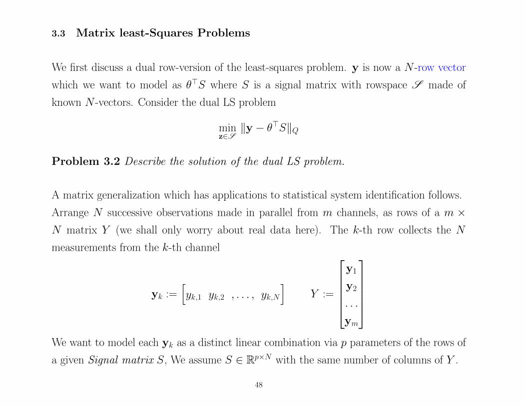
Arrange N successive observations made in parallel from m channels, as rows of a m ×N matrix Y (we shall only worry about real data here). The k-th row collects the N
measurements from the k-th channel
yk :=[yk,1 yk,2 , . . . , yk,N
]Y :=
y1
y2
. . .
ym
We want to model each yk as a distinct linear combination via p parameters of the rows of
a given Signal matrix S, We assume S ∈ Rp×N with the same number of columns of Y .
48
One may then generalize the standard LS problem to matrix-valued data as follows.
Let Y ∈ Rm×N and S ∈ Rp×N be known real matrices and consider the problem
minΘ∈Rm×p
‖Y − ΘS ‖F , (Frobenius norm) (3.12)
where Θ ∈ Rm×p is an unknown matrix parameter.
The Frobenius norm could actually be weighted by a positive definite weight matrix Q.
The problem can be solved for each row yk by the orthogonality principle. Let S be the
rowspace of S and denote by θkS ; θk ∈ Rp a vector in S . Then the optimality condition
is
yk − θkS ⊥ S ; i.e. ykQS> = θkSQS
> k = 1, 2, . . . ,m
so that, assuming S of rank m, the solution is
Θ = Y QS> [SQS>]−1 .
49
3.4 A problem from subspace identification
Assume you observe the trajectories of the state, input and output variables of a linear
MIMO stationary stochastic system[x(t + 1)
y(t)
]=
[A B
C D
] [x(t)
u(t)
]+
[K
J
]w(t)
where w is white noise. With the observed trajectories from some time t onwards one
constructs the data matrices (all having N + 1 columns)
Yt := [ yt, yt+1, yt+2, . . . , yt+N ] Ut := [ ut, ut+1, ut+2, . . . , ut+N ]
Xt := [ xt, xt+1, xt+2, . . . , xt+N ]q Xt+1 := [ xt+1, xt+2, . . . , xt+N+1]
If the data obey the linear equation above, there must exist a corresponding white noise
trajectory Wt := [ wt, wt+1, wt+2, . . . , wt+N ] such that[Xt+1
Yt
]=
[A B
C D
][Xt
Ut
]+
[K
J
]Wt
From this model one can now attempt to estimate the matrix parameter Θ :=
[A B
C D
]based on the observed data. This leads to a matrix LS problem of the kind formulated in
the previous page. In practice the state trajectory is not observable and must be previously
estimated from input-output data.
50
3.5 Relation with Left- and Right- Inverses
It is obvious that A = [S>QS ]−1 S>Q is a left-inverse of S; i.e. AS = I for any
non-singular Q. Left- and right-inverses are related to least-squares problems.
Let A ∈ Rm×n and let Q1 and Q2 be symmetric positive definite. Consider the following
weighted least-squares problems
If rankA = n, minx∈Rn
‖Ax− b2‖Q2 (3.13)
If rankA = m, miny∈Rm
‖A>y − b1‖Q1 (3.14)
where b1 ∈ Rn, b2 ∈ Rm are fixed column vectors. From formula (3.10) (and its dual) we
get:
Proposition 3.1 The solution to Problem (3.13) can be written as x = A−Lb2 where
A−L is the left-inverse given by
A−L = [A>Q2A ]−1A>Q2 ,
while that of Problem (3.14) can be written as y> = b>1 A−R where A−R is the right-
inverse given by
A−R = Q1A>[AQ1A
> ]−1 .
51
Conversely, we can show that any left- or right-inverse admits a representation as a solution
of a weighted Least-Squares problem.
Proposition 3.2 Assume rankA = n and let A−L be a particular left-inverse of A.
Then there is a Hermitian positive-definite matrix Q such that
A−L = [ A>QA ]−1A>Q (3.15)
and, in case rankA = m, a dual statement holds for an arbitrary right inverse.
Proof. The property of being a left-inverse is independent of the metrics on Cm and Cn.
Hence we may assume Euclidean metrics. Since A has linearly independent columns we can
write A = RA where A> := [I 0]> and R ∈ Cm×m is invertible. Any left inverse A−L
must be of the form A−L = [I T ] with T arbitrary. There exist a square matrix Q such
that(A>QA
)= Q11 is invertible and(
A>QA)−1
A>Q = [I T ] = A−L.
In fact, just let T = Q−111 Q12, which is clearly still arbitrary. Without loss of generality we
may actually choose Q11 = I , Q12 = T .
52
To get a representation of A−L of the form (3.15) to hold, we just need to make sure that
there exists Q so that, Q = Q> > 0. To this end we may just choose Q21 = Q>12 and
Q22 = Q>22 > Q21Q−111 Q12.
In general, A−LA = I means that A−LRA = I ; i.e. A−LR is a left inverse of A; that is
A−LR = A−L =(A>QA
)−1A>Q =
=[A>(R>)−1QR−1A
]−1A>(R>)−1Q
(3.16)
and, renaming Q := (R>)−1QR−1 we get A−L =(A>Q A
)−1A>Q. Since R is invertible
Q can be taken to be Hermitian and positive definite. The statement is proved.
Problem 3.3 For a fixed A of full column rank the left inverses can be parametrized
in terms of Q. Is this parametrization 1:1 ?
The full-rank condition simplifies the discussion but is not essential. First, when rankS < p
but still p ≤ N , the model can be reparametrized by using a smaller number of parameters.
Problem 3.4 Show how to reparametrize in 1:1 way a model with rankS < p but still
p ≤ N .
53
3.6 The Pseudoinverse
For an arbitrary A, the least squares problems (3.13), (3.14) have no unique solution. When
(3.9) does not hold one can bring in the pseudoinverse of S>QS. The following definition
is for arbitrary weighted inner-product spaces.
Consider a linear map between finite-dimensional inner product spaces A : X → Y . For
concreteness may think of A as a m×n (in general complex) matrix and the spaces endowed
with weighted inner products 〈x1, x2〉Cn = x>1 Q1x2 and 〈y1, y2〉Cm = y>1 Q2y2 where Q1, Q2
are Hermitian positive definite matrices.
Recall the basic fact which holds for arbitrary linear operators on finite-dimensional inner
product spaces A : X → Y .
Lemma 3.1 We have
X = ker(A)⊕ Im (A∗) , Y = Im (A)⊕ ker(A∗) . (3.17)
where the orthogonal complements and the adjoint are with respect to the inner prod-
ucts in X and Y .
Below is a key observation for the introduction of generalized inverses of a linear map.
54
Proposition 3.3 The restriction of A to the orthogonal complement of its nullspace
(kerA)⊥ = ImA∗ is a bijective map onto its range ImA.
Proof. Let y1 be an arbitrary element of Im (A) so that y1 = Ax for some x ∈ Cn and
let x = x1 + x2 be relative to the orthogonal decomposition Cn = ker(A) ⊕ ImA∗. Then
there is an x2 such that y1 = Ax2. This x2 ∈ ImA∗ must be unique since A(x′2 − x′′2) = 0
implies x′2−x′′2 ∈ ker(A) which is orthogonal to ImA∗ so that it must be that x′2−x
′′2 = 0.
Therefore the restriction of A to ImA∗ is injective.
Hence the restriction of A to Im (A∗) is a map onto Im (A) which has an inverse. This
inverse can be extended to the whole space Y by making its kernel equal to the orthog-
onal complement of Im (A). The exension is called the Moore-Penrose generalized
inverse or simply the pseudo-inverse of A and is denoted A†.
Proposition 3.4 The pseudoinverse A† is the unique linear transformation Y →X
which satisfies the following two conditions
x ∈ Im (A∗)⇒ A†Ax = x (3.18)
y ∈ ker(A∗)⇒ A†y = 0 . (3.19)
Moreover
ImA† = ImA∗, ker(A†) = ker(A∗) (3.20)
55
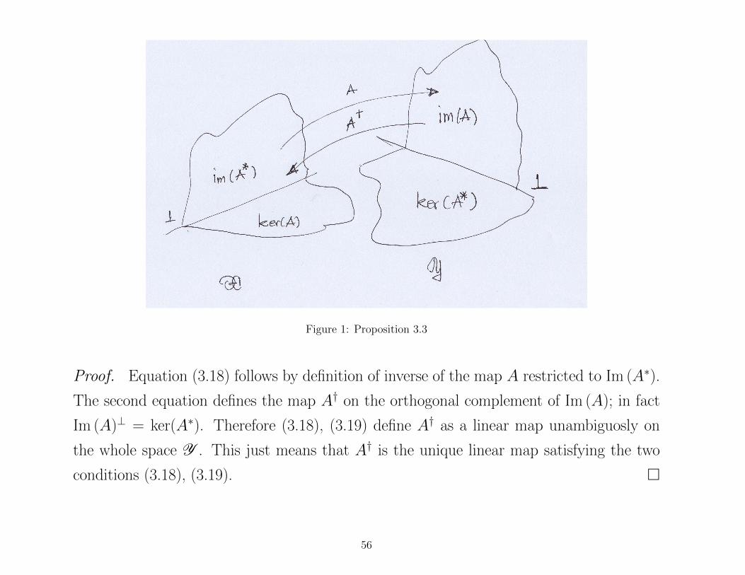
Figure 1: Proposition 3.3
Proof. Equation (3.18) follows by definition of inverse of the map A restricted to Im (A∗).
The second equation defines the map A† on the orthogonal complement of Im (A); in fact
Im (A)⊥ = ker(A∗). Therefore (3.18), (3.19) define A† as a linear map unambiguosly on
the whole space Y . This just means that A† is the unique linear map satisfying the two
conditions (3.18), (3.19).
56
Corollary 3.1 Let A ∈ Cm×n be block-diagonal: A = diag A1, 0 where A1 ∈ Cp×p , p < n
is invertibile. Then, irrespective of the inner product in Cn,
A† =
[A−1
1 0
0 0
]. (3.21)
Problem 3.5 Prove Corollary 3.1. (Hint: identify the various subspaces and use the
basic relations (3.18), (3.19).)
The following facts follow from (3.18), (3.19).
Proposition 3.5 1. A†A and AA† are self-adjoint maps.
2. A†A is the orthogonal projector of X onto Im (A∗).
3. I − A†A is the orthogonal projector of X onto ker(A).
4. AA† is the orthogonal projector of Y onto Im (A).
5. I − AA† is the orthogonal projector of Y onto ker(A∗).
Proof. Let x = x1 + x2 be the orthogonal decomposition of x induced by X = ker(A)⊕Im (A∗). To prove (1) take any x, z ∈ X and note that by (3.18), 〈z, A†Ax〉X =
57
〈z, A†Ax2〉X = 〈z2, x2〉X = 〈A†Az2, x〉X = 〈A†Az, x〉X .
2. Clearly A†A is idempotent since by (3.18) A†Ax = A†Ax2 = x2 and hence A†AA†Ax =
A†Ax2 = A†Ax. Same is obviously true for AA†. Hence by (1) A†A is an orthogonal
projection onto Im (A∗).
To prove (3) and (5) let, dually, b = b1 + b2 be the orthogonal decomposition of b ∈ Y =
ker(A∗)⊕ Im (A), then, by (3.19)
AA†b = AA†b2 = b2 .
since A is the inverse of A† restricted to Im (A).
Problem 3.6 Describe the pseudoinverse of an orthogonal Projection P : X→ Y
58
Certain properties of the inverse are shared by the pseudoinverse only to a limited extent.
Products: If A ∈ Rm×n, B ∈ Rn×p the product formula
(AB)† = B†A†
is generally not true. It holds if
• A has orthonormal columns (i.e. A∗A = In ) or,
• B has orthonormal rows (i.e.BB∗ = In ) or,
• A has all columns linearly independent (full column rank) and B has all rows linearly
independent (full row rank).
The last property yields the solution to
Problem 3.7 Let A ∈ Rn×m with rank(A) = r. Consider a full rank factorization of
the form A = LR with L ∈ Rn×r, R ∈ Rr×m. Prove that
A+ = R>(L>AR>)−1L>
Problem 3.8 Prove that [A†]∗ = [A∗]†
Show that the result below is not true for arbitrary invertible maps (matrices) T1, T2.
59
Proposition 3.6 Let A : X → Y and T1 : X → X1 and T2 : Y → Y2, be unitary
maps; i.e. T1T∗1 = I , T2T
∗2 = I. Then
(T1AT2)† = T−12 A†T−1
1 = T ∗2A†T ∗1 . (3.22)
Problem 3.9 Show that
A+ = (A∗A)+A∗ , A+ = A∗(AA∗)+
and thereby prove the product formulas
A+(A∗)+ = (A∗A)+ , (A∗)+A+ = (AA∗)+
60
Least Squares and the Moore-Penrose pseudo-inverse
The following result provides a characterization of the pseudoinverse in terms of least-
squares.
Theorem 3.1 The vector x0 := A†b is the minimizer for the least-squares problem
minx∈Rn
‖Ax− b‖Q2
which has minimum ‖ · ‖Q1-norm.
Proof. Let V (x) := ‖Ax− b‖2Q2
and L,M be square matrices such that L>L = Q1 and
M>M = Q2. By defining x := Lx and scaling A and b according to A := MAL−1, b :=
Mb we can rephrase our problem in Euclidean metrics and rewrite V (x) as ‖Ax − b‖2
where ‖ · ‖ is the Euclidean norm. Further, let
x = x1 + x2, x1 ∈ ker(A), x2 ∈ Im (A>) (3.23)
b = b1 + b2 b1 ∈ Im (A), b2 ∈ ker(A>) (3.24)
61
be the orthogonal sum decompositions according to (3.17). Now V (x)− V (x0) is equal to
V (x)− V (x0) = ‖A(x1 + x2)− (b1 + b2)‖2 − ‖Ax0 − (b1 + b2)‖2
= ‖(Ax2 − b1)− b2‖2 − ‖(Ax0 − b1)− b2‖2
= ‖Ax2 − b1‖2 + ‖b2‖2 −(‖Ax0 − b1‖2 + ‖b2‖2
)= ‖Ax2 − b1‖2 − ‖AA†(b1 + b2)− b1‖2
= ‖Ax2 − b1‖2 ≥ 0
the last equality following from proposition 3.4. Hence x0 = L−1x0 is a minimum point
of V (x). However all x = x1 + x2 such that Ax2 − b1 = 0 are also minimum points. For
all these solutions it must however hold that x2 = x0, for, A(x2 − x0) = 0 implies that
x2 − x0 ∈ ker(A) so that x2 − x0 must be zero.
Hence ‖x‖2 = ‖x1 + x2‖2 = ‖x1 + x0‖2 = ‖x1‖2 + ‖x0‖2 ≥ ‖x0‖2 which is by definition
equivalent to ‖x‖2Q1≥ ‖x0‖2
Q1.
62
3.7 The Euclidean pseudoinverse
Below is the classical definition of pseudoinverse of a matrix.
Theorem 3.2 The (Euclidean) Moore-Penrose pseudoinverse, A+, of a real (or com-
plex) matrix A ∈ Rn×m is the unique matrix satifying the four conditions:
1. AA+A = A
2. A+AA+ = A+
3. A+A is symmetric (resp. Hermitian)
4. AA+ is symmetric (resp. Hermitian)
Proof. The proof of existence is via the Singular Value Decomposition; see Theorem 3.6.
Proof of Uniqueness: Let A+1 , A+
2 be two matrices satisfying 1.,2.,3.,4. Let D := A+1 −A+
2 .
Then
1. ⇒ ADA = 0. 4. ⇒ A∆ = AA+1 − AA+
2 symmetric ⇒ AD = D>A> ⇒ D>A>A = 0
⇒ A>AD = 0 ⇒ D ∈ ker(A>A) = ker(A) (columns).
2.+3. ⇒ A>(A+1 )>A+
1 = A+1 and A>(A+
2 )>A+2 = A+
2 ⇒ A>(A+1 )>A+
1 −A>(A+2 )>A+
2 = D
⇒ D = A>[(A+1 )>A+
1 − (A+2 )>A+
2 ] ∈ Im (A>) = [ker(A)]⊥ ⇒ D = 0.
63
3.8 The Pseudoinverse and Orthogonal Projections
The proposition below is the Euclidean version of Proposition 3.5.
Proposition 3.7 Let A ∈ Rn×m.
1. AA+ is the orthogonal projection onto Im (A).
2. A+A is an orthogonal projection onto Im (A>).
3. I − AA+ projects onto [Im (A)]⊥ = ker(A>).
4. I − A+A projects onto [Im (A>)]⊥ = ker(A).
Proof.
1. (AA+)2 = AA+AA+ = AA+. Moreover AA+ is symmetric, Problem 3.19.
Im (AA+) ⊆ Im (A). Conversely, Im (A) = Im (AA+A) ⊆ Im (AA+).
2. Similar proof: Im (A+A) = Im (A>(A>)+) and 2. ⇒ Im (A>(A>)+) = Im (A>).
3. and 4. Follow from 1. and 2.
These projections are all related to least squares problems.
64
Problem 3.10 Assume A as a m × n (in general complex) matrix acting on spaces
endowed with weighted inner products 〈x1, x2〉Cn = x>1 Q1x2 and 〈y1, y2〉Cm = y>1 Q2y2
where Q1, Q2 are Hermitian positive definite matrices. Denote by A+ the Euclidean
pseudoinverse of A. What is the relation between A† and A+?
Solution: Let T1 : X → Cn and T2 : Y → Cm and L,M be square matrices such that
L>L = Q1 and M>M = Q2 so that T1 : x 7→ Lx and T2 : y 7→ My are unitary maps
onto Euclidean spaces, T1 : X → Cn and T2 : Y → Cm. Since T1x = Lx it follows from
(1.4) that T ∗1 ξ = Q−11 L> = L−1 and similarly T ∗2 = M−1. Now, the action of A can be
decomposed as
X → CnA︷︸︸︷→ Cm → Y
for a certain matrix A : Cn → Cm, we have A = T1AT−12 but T2 is self adjoint; i.e.
T−12 = T ∗2 and hence formula (3.22) holds. Hence
A† ≡ A+ = M−1A†L
65
3.9 Linear equations
Let A ∈ Rn×m, B ∈ Rn×p. Consider the equation
AX = B (3.25)
Theorem 3.3 1. Equation (3.25) admits solutions iff B ∈ Im (A) (Im (B) ⊆ Im (A)).
2. If equation (3.25) admits solutions, all its solutions are given by:
X = A+B + (I − A+A)C, (3.26)
for an arbitrary C ∈ Rm×p.
Proof. In fact, if B ∈ Im (A) then ∃ Y such that B = AY .
Let X = A+B + (I − A+A)C = A+AY + (I − A+A)C
⇒ AX = AA+AY + A(I − A+A)C = AY + 0 = B.
Conversely, let Z be a solution of (3.25) and ∆ := Z − A+B
then A∆ = AZ − AA+B = AZ − B = 0 ⇒ ∆ ∈ ker(A) = [Im (A>)]⊥ = [Im (A+)]⊥ =
[Im (A+A)]⊥ = Im (I − A+A) ⇒ ∃ C s.t. ∆ = (I − A+A)C.
66
Let A ∈ Rn×m, B ∈ Rn×p. Assume that AX = B admits solutions.
What is the meaning of X = A+B ?
Example: let p = 1 (i.e. X = x ∈ Rm and B = b ∈ Rn are vectors):
Ax = b (3.27)
The solutions of this equation are all of the form
x = A+b + (I − A+A)c
where the two terms are orthogonal, then
‖x‖2 = [b>(A+)> + c>(I − A+A)>][A+b + (I − A+A)c] = b>(A+)>A+b + c>(I − A+A)2c
= ‖A+b‖2 + ‖(I − A+A)c‖2
Hence x = A+b is the minimum norm solution of (3.27).
For p > 1 use the Frobenius norm of a matrix X : ‖X‖F :=√
tr (X>X) (note that
‖X‖F =√∑
ijX2ij).
Since the solutions of (3.25) are all of the form X = A+B + (I − A+A)C
‖X‖2F = ‖A+B‖2
F +‖(I−A+A)C‖2F ⇒ X = A+B is the minimum norm solution .
67
3.10 Unfeasible linear equations and Least Squares
Let A ∈ Rn×m, B ∈ Rn×p and assume B 6∈ Im (A).
Then 6 ∃ X solving the equation AX = B.
May solve the equation in the (approximate) least squares sense (MATLAB).
Problem 3.11 Find X minimizing ‖AX −B‖F
Consider again the case p = 1 (minimize ‖Ax− b‖).For all x ∈ Rm ∃y ∈ Rn such that Ax = AA+y (generalizes Sθ = Py)
⇒ Ax− b = AA+y − b = AA+(y − b + b)− b = AA+(y − b)︸ ︷︷ ︸∈Im (A)
+︸︷︷︸⊥
[−(I − AA+)b]︸ ︷︷ ︸∈[Im (A)]⊥
⇒ ‖Ax− b‖2 = ‖AA+(y − b)‖2 + ‖(I − AA+)b‖2
Now y = b is a solution of the LS problem
miny
[‖AA+(y − b)‖2 + ‖(I − AA+)b‖2]
Hence x = A+b is a solution of minx ‖Ax− b‖2 and minx ‖Ax− b‖2 = ‖(I −AA+)b‖2.
Proposition 3.8 For p = 1, x = A+b is the solution to Problem 3.11 of minimum
norm.
68
Problem 3.12 Prove the minimum norm property. Compare with Theorem 3.1. Are
we repeating the same proof?
For p > 1 the computations are the same:
Proposition 3.9 X = A+B is the solution of Problem 3.11 of minimum Frobenius
norm.
Problem 3.13 Parametrize all solutions to Problem 3.11.
69
3.11 The Singular value decomposition (SVD)
We shall first do the SVD for real matrices. In Section 3.14 we shall generalize to general
linear maps in inner product spaces.
Problem 3.14 Let A ∈ Rm×n and r := minn,m. Show that AA> and A>A share
the first r eigenvalues. How are the eigenvectors related?
Theorem 3.4 Let A ∈ Rm×n of rank r ≤ min(m,n). Can find two orthogonal matri-
ces U ∈ Rm×m and V ∈ Rn×n and positive numbers σ1 ≥, . . . ,≥ σr, the singular
values of A, so that
A = U∆V > ∆ =
[Σ 0
0 0
], Σ = diag σ1, . . . , σr (3.28)
Let U =[Ur Ur
], V =
[Vr Vr
]where the submatrices Ur, Vr keep only the first r
columns of U, V . We get a Full-rank factorization of A
A = Ur ΣVr = [u1, . . . , ur] Σ [v1, . . . , vr]>
where
U>r Ur = Ir = V >r Vr, but UrU>r 6= Im, VrV
>r 6= In .
70
Proof is based on eigenvalue-eigenvector decomposition of the symmetric matrices AA> and
A>A. See the next section for the full proof. Here we do a verification. Assume that (3.28)
holds. Then
AA> = U∆2U> ; A>A = V∆2V >
hence U = [u1, . . . , um] = normalized eigenvectors of AA>;
and V := [v1, . . . , vn] = normalized eigenvectors of A>A
while σ21 ≥, . . . ,≥ σ2
r are the (non zero) eigenvalues of AA> (or of A>A). Since
Ax = U
[Σ 0
0 0
] [V >r
V >r
]x = Ur ΣV >r x
where Σ > 0, we have Ax = 0 ⇐⇒ V >r x = 0 ⇐⇒ x ∈ span Vr. Dyad formulas
Ax =
r∑k=1
uk σk〈vk , x〉 , A>y =
r∑k=1
vk σk〈uk , y〉
In particular on the singular vectors A acts like multiplication by a rank one matrix
Avj =
r∑k=1
uk σk〈vk , vj〉 = σj uj , A> uj =
r∑k=1
vk σk〈uk , uj〉 = σj vj (3.29)
can be seen as a far reaching generalization of spectral decomposition of symmetric matrices.
71
3.12 Useful Features of the SVD
Range and Nullspace of A:
Im (A) = Im (Ur) = span ([u1, . . . , ur]), [Im (A)]⊥ = Im (Ur)
ker (A) = Im (V ⊥r ) = span ([vr+1, . . . , vn]) [ker (A)]⊥ = Im (Vr)
Approximation properties: the matrix
Ak :=
k∑i=1
σi ui v>i , k ≤ n
is the best approximant of rank k of A:
minrank (B)=k
‖A−B‖2 = ‖A− Ak‖2 = σk+1
minrank (B)=k
‖A−B‖2F = ‖A− Ak‖2
F = σ2k+1 + . . . + σ2
r
72
3.13 Matrix Norms
Let A ∈ Rn×m. For now Rm and Rn are equipped with the inner product 〈u, v〉 := u>v
inducing the Euclidean norm ‖u‖ :=√u>u.
The Euclidean norms on Rm and Rn induce a norm on the set of linear maps from Rm to
Rn which is defined as follows:
‖ · ‖2 : Rn×m −→ R+ , ‖A‖2 := supv 6=0
‖Av‖‖v‖
The definition is quite general and applies to linear maps between arbitrary inner product
spaces. If A ∈ Rn×m it descends from Schwarz inequality u>v ≤ ‖u‖‖v‖ that there is a
constant k such that ‖Av‖ ≤ k‖v‖. The 2-norm of A is in fact the largest such k.
Problem 3.15 Let A ∈ Rn×m. Show that:
1.The sup in the definition of the induced norm is indeed a max, i.e.
‖A‖2 = maxv 6=0
‖Av‖‖v‖
and ‖A‖2 = max‖v‖=1
‖Av‖
2. ‖A‖2 is equal to σ1, the first (i.e. the largest) singular value of A. For this reason
this norm is also called spectral norm.
The second question relates to the very instructive maximization of the so-called Rayleigh
quotients.
73
The solution of the following problem follows instead quite trivially from tr (A) =∑λk(A).
Problem 3.16 The Frobenius norm ‖A‖F defined in (1.2) is given by
‖A‖2F =
∑i,j
a2i,j = σ2
1 + . . . + σ2r .
Denote by Σ(A) the set of singular values of A.
Problem 3.17 Let A be square. Show that:
1. If A = A> ≥ 0 then Σ(A) = σ(A).
2. 0 ∈ σ(A) ⇐⇒ 0 ∈ Σ(A).
3. If A = A> then Σ(A) = |s| : s ∈ σ(A).4. σ(A) and Σ(A) can be quite different (discuss the intersection σ(A) ∩ Σ(A)).
5. What are the singular values of a skew-symmetric matrix?
If a matrix A is far from being symmetric (in fact far from normal), for example if A is
lower triangular, then the singular values can be very different from the eigenvalues. Give
some examples.
74
3.14 Generalization of the SVD
Let X , Y be finite-dimensional inner product spaces of dimensions n and m.
Lemma 3.2 Let Q : Rn → V be a unitary map. Then dim V = n and there is an
orthonormal basis u1, . . . , un in V suchthat Qx =∑ukξk where ξk = coordinates of x.
Proof: Let ek be a canonical basis in Rn and Qek := uk, k = 1, . . . , n. Then the uk
form an orthonormal basis. By linearity Q∑ξkek =
∑ξkQek.
Theorem 3.5 Let A : X → Y of rank r ≤ min(m,n). There are two unitary maps
U : Rm → Y , V : Rn → X and a sequence of positive real numbers ordered in
decreasing magnitude, σ1 ≥ . . . ≥ σr, called the singular values of A, such that
A = U∆V ∗ , ∆ =
[Σ 0
0 0
], Σ = diag σ1, . . . , σr (3.30)
The matrix U = [u1, . . . , um] , uk ∈ Y is made by the the normalized eigenvectors of
AA∗; dually, the columns of V := [v1, . . . , vn] , vk ∈X are the normalized eigenvectors
of A∗A. The squared singular values σ21 ≥ . . . ≥ σ2
r are the non-zero eigenvalues of
AA∗ ( or A∗A).
75
Proof. Let [v1, . . . , vn], be normalized eigenvectors of A∗A so that
A∗Avk = σ2kvk k = 1, . . . n
with A∗Avk = 0 for k > r. Note that these last eigenvectors are essentially arbitrary in the
nullspace of A. Multiplying from the left by A one gets
AA∗(Avk) = σ2k(Avk) k = 1, . . . n
so the vectors
uk :=1
σkAvk k = 1, . . . r ,
are normalized eigenvectors of AA∗. In fact,
〈uk, uj〉 =〈vk, A∗Avj〉
σkσj=
σ2j
σkσj〈vk, vj〉 =
σ2j
σkσjδkj
Completing the family u1, . . . , ur with m− r (eigen)vectors in the nullspace of AA∗ we
obtain an orthonormal basis in Y . Then
〈uk, Avj〉 =〈vk, A∗Avj〉
σk=σ2j
σk〈vk, vj〉 =
σ2j
σkδkj
for k, j ≤ r and 〈uk, Avj〉 = 0 otherwise. These relations are equivalent to U ∗AV = ∆.
The following full-rank SVD factorization of A is obtained by eliminating all the zero
blocks in (3.30)
A = [u1, . . . , ur] Σ [v1, . . . , vr]∗ := U1ΣV ∗1 (3.31)
76
where Σ = diag σ1, . . . , σr and U1, V1 are the submatrices obtained by keeping only the
first r columns of U and V . Note that U1 and V1 still have orthonormal columns
U ∗1U1 = Ir = V ∗1 V1 .
Corollary 3.2 The image space and the nullspace of A are :
Im (A) = Im (U1) = span u1, . . . , ur, ker(A) = ker(V ∗) = span vr+1, . . . , vn
Moreover, the 2-norm and the Frobenius norms of A are
‖A‖2 = ‖Σ‖2 = σ1, ‖A‖2F = ‖Σ‖2
F = σ21 + . . . + σ2
r
The map
Ak :=
k∑i=1
σiui 〈vi, · 〉 k ≤ r
is the best rank k(≤ r) approximation of A in a variety of norms; in fact,
minB ; rank (B)=k
‖A−B‖2 = ‖A− Ak‖2 = σk+1 (3.32)
and
minB ; rank (B)=k
‖A−B‖2F = ‖A− Ak‖2
F = σ2k+1 + . . . + σ2
r (3.33)
77
Note that (A − Ak)x =∑r
i=k+1 σiui 〈vi, x 〉 and hence ‖A − Ak‖2 = σk+1. A similar
argument holds for the Frobenius norm.
The proof that Ak is the actual minimizer is tricky. See [Golub-Van Loan] p. 19-20.
Problem 3.18 Is the SVD of A unique? discuss the case where there are multiple
eigenvalues of AA∗ (or of A∗A). Assume that the σi’s are all distinct. Is the SVD
unique in this case?
Let A = Udiag σ1, . . . , σnV ∗ where U and V are arbitrary orthonormal matrices and
σ1 ≥ . . . ≥ σn ≥ 0. Is this necessarily the SVD of A ? In any case, are σ1, . . . σn the
singular values of A ?
There is an equivalent statement where the singular values are p = min(n,m) but some of
them (σr+1, . . . , σp) are allowed to be zero.
78
3.15 SVD and the Pseudoinverse
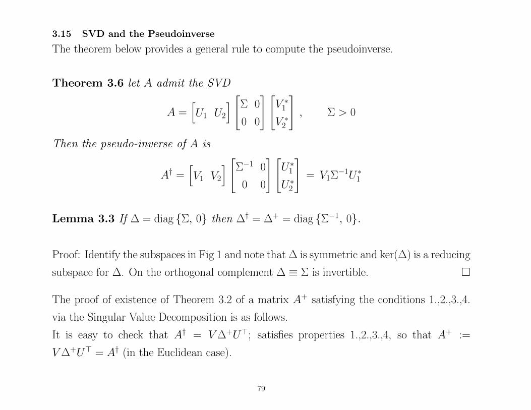
The theorem below provides a general rule to compute the pseudoinverse.
Theorem 3.6 let A admit the SVD
A =[U1 U2
] [Σ 0
0 0
][V ∗1
V ∗2
], Σ > 0
Then the pseudo-inverse of A is
A† =[V1 V2
] [Σ−1 0
0 0
][U ∗1
U ∗2
]= V1Σ−1U ∗1
Lemma 3.3 If ∆ = diag Σ, 0 then ∆† = ∆+ = diag Σ−1, 0.
Proof: Identify the subspaces in Fig 1 and note that ∆ is symmetric and ker(∆) is a reducing
subspace for ∆. On the orthogonal complement ∆ ≡ Σ is invertible.
The proof of existence of Theorem 3.2 of a matrix A+ satisfying the conditions 1.,2.,3.,4.
via the Singular Value Decomposition is as follows.
It is easy to check that A† = V∆+U>; satisfies properties 1.,2.,3.,4, so that A+ :=
V∆+U> = A† (in the Euclidean case).
79
Problem 3.19 Prove that
1. (A+)+ = A.
2. (A+)> = (A>)+.
3. If A ∈ Rn×n and TT> = T>T = I, then (T>AT )+ = T>A+T .
Problem 3.20 Let A be square. Prove that
1. A+ is singular ⇔ A is singular.
2. If A is singular and A>v = 0 ⇒ A+v = 0.
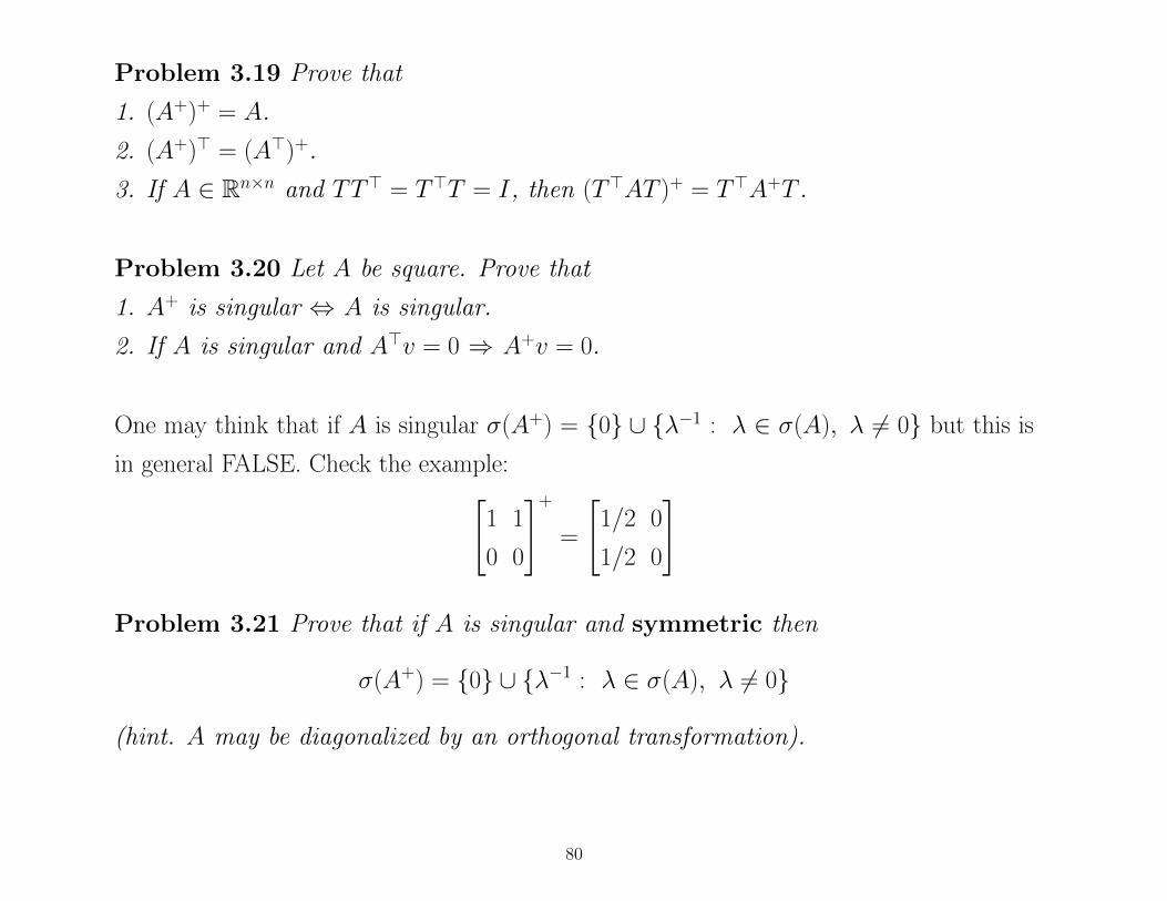
One may think that if A is singular σ(A+) = 0 ∪ λ−1 : λ ∈ σ(A), λ 6= 0 but this is
in general FALSE. Check the example:[1 1
0 0
]+
=
[1/2 0
1/2 0
]
Problem 3.21 Prove that if A is singular and symmetric then
σ(A+) = 0 ∪ λ−1 : λ ∈ σ(A), λ 6= 0
(hint. A may be diagonalized by an orthogonal transformation).
80
4 NUMERICAL ASPECTS OF L-S PROBLEMS
Solving the normal equations
S>QS θ = S>Qy
could be problematic for large dimensional problems. Numerical errors in the data could
be dramatically amplified in the solution ! Need to be aware of when/why problems may
arise and of possible solutions.
Most computational problems can be formalized in the following way: one has a function
say f : Rk → Rp defined mathematically and a k-dimensional vector of “data” α. One
wants to compute x = f (α). For example one may want to solve numerically a linear
system
Ax = b , (4.34)
Here the data are α = (A, b) and the function f is defined mathematically by the expression
f (α) = A−1 b.
81
Now there are two main aspects of the problem to be taken into account.
A) The data, α, are always represented in the computer by a finite arithmetics and hence
real-valued data are affected by rounding errors. In the computer you can only store
α + δα, where δα is the rounding error, not α.
B) In general there are no algorithms which implement exactly the function f or even if
exact procedures are available , it may be inconvenient or uneconomical to use them.
In practice f is computed approximately; the algorithm implements an approximation,
say, g(·), of f (·).
These are of course two distinct causes of errors which, however, always tend to sum up.
Nevertheless it is convenient to discuss them separately.
Definition 4.1 The numericalproblem x = f (α) is ill-conditioned if small percent-
age errors on α generate large percentage error on the solution x. In other terms,
letting x = f (α) and x + δx = f (α + δα) one has
‖δx‖‖x‖
‖δα‖‖α‖
. (4.35)
82
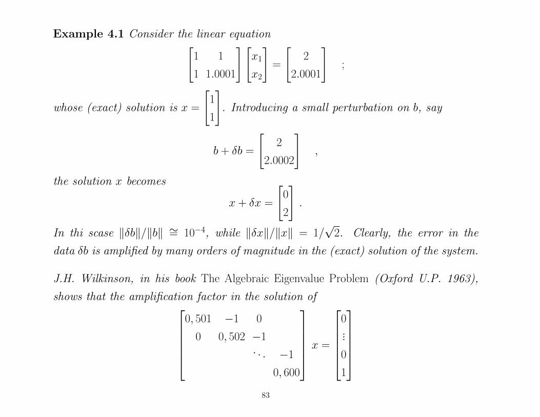
Example 4.1 Consider the linear equation[1 1
1 1.0001
][x1
x2
]=
[2
2.0001
];
whose (exact) solution is x =
[1
1
]. Introducing a small perturbation on b, say
b + δb =
[2
2.0002
],
the solution x becomes
x + δx =
[0
2
].
In thi scase ‖δb‖/‖b‖ ∼= 10−4, while ‖δx‖/‖x‖ = 1/√
2. Clearly, the error in the
data δb is amplified by many orders of magnitude in the (exact) solution of the system.
J.H. Wilkinson, in his book The Algebraic Eigenvalue Problem (Oxford U.P. 1963),
shows that the amplification factor in the solution of0, 501 −1 0
0 0, 502 −1. . . −1
0, 600
x =
0...
0
1
83
is of the order of 1022 !
N.B. Ill-conditioning is an intrinsic characteristic of a numerical problem which cannot be
modified by the use of special or “specially smart” algorithms. Errors due to ill-conditioning
cannot be reduced or modified by the algorithm used to implement the computation of
x = f (α). Nevertheless a well-conditioned problem can be “ruined” by a poor algorithm.
Intuitively a “good” algorithm should perturb the theoretical f so little that the perturba-
tion could well be attributed to rounding errors in the data.
Definition 4.2 An algorithm g fo rthe numerical problem x = f (α), is numerically
stable if for every α ∈ Rk there is a perturbation δα, of the same order of magnitude
of the underlying rounding errors, such that f (α+δα) differs from g(α) percentagewise
of a quantity of the same order of f (α + δα)− f (α).
In other words, the errors introduced by a numerically stable algorithm can always be
attributed to errors due to the finite precision arithmetics. In other words, g is numerically
stable if the computed solution y = g(α) can in principle be obtained by an “exact solver”
using perturbed data, namely y = f (α + δα) where ‖δα‖/‖α‖ is of the same order of the
underlying rounding errors.
84
Clearly no algorithm, no matter how numerically stable, can provide ac-
curate solutions to an ill-conditioned problem. An unstable algorithm can
however easily destroy a well-conditioned problem.
Remark 4.1 In Numerical Linear Algebra the perturbations considered are due to
finite precision arithmetics (rounding errors) however the theory which follows does
not depend at all on this interpretation and the perturbations on the data may have
in fact any origin, say measurement noise or approximation errors of various kinds.
85
4.1 Numerical Conditioning and the Condition Number
The normal equations are a special case of the ubiquitous linear system Ax = b. So we
shall first discuss this problem assuming for the moment that A ∈ Rn×n is nonsingular so
that the solution of this problem is well-defined.
Assume for the moment that A has no perturbations (δA = 0); say can be stored exactly in
the computer. Want to get an estimate of how much the relative error on the data ‖δb‖/‖b‖influences ‖δx‖/‖x‖. For this purpose we shall use Euclidean norms
Recall that ‖A‖ (normally denoted ‖A‖2 when there is danger of confusion) is the smallest
number k > 0 for which the inequality ‖Ax‖ ≤ k ‖x‖ holds. It can be computed as follows:
‖A‖2 = supx 6=0
x>A>Ax
x>x. (4.36)
the second member is known as a Rayleigh quotient and is actually equal to maximal
eigenvalue of A>A, hence to the square of the maximal singular value of A:
‖A‖2 = maxi
λi(A>A) = σ2
1(A) (4.37)
Problem 4.1 Prove this equality.
86
From the relations x = A−1 b and b = Ax one easily gets the estimates ‖δx‖ ≤ ‖A−1‖‖δb‖and ‖x‖ ≥ ‖A‖−1‖b‖, so that
‖δx‖‖x‖
≤ ‖A‖ ‖A−1‖ ‖δb‖‖b‖
(4.38)
The number c(A) := ‖A‖ ‖A−1‖ can be interpreted as an amplification gain of the errors
on the right hand side of the linear system Ax = b. It is called condition number of
the problem Ax = b (or, of the matrix A). As we shall see in a moment, c(A) has a more
general meaning. First, let us observe that from I = AA−1 it follows that
1 = ‖I‖ ≤ ‖A‖ ‖A−1‖ = c(A)
so that c(A) is always an amplification coefficient.
Recalling
‖A‖2 = λMAX (A>A) , ‖A−1‖2 = λMAX (A−>A−1) = λMAX (AA>)−1 =1
λMIN(AA>)
one immediately sees that
c2(A) =λMAX(A>A)
λMIN(A>A)=σ2
1(A)
σ2n(A)
(4.39)
in particular when A is symmetric,
c(A) =λMAX(A)
λMIN(A). (4.40)
87
From this formula one sees that when A is nearly singular the minimum singular value
is near zero and c(A) may become large. However this is not always the case since for
example A = εI with ε→ 0 has numerical conditioning equal to one. In any case the best
conditioned matrices are those for which A>A = αI . In this case one has c(A) = 1. These
matrices are sometimes called orthogonal while those for whichAA> = I are orthonormal.
Orthogonal matrices play a fundamental role in Numerical Linear Algebra.
Problem 4.2 Compute the numerical conditioning of the 2 × 2 matrix in Example
4.1.
Problem 4.3 Assume that A is symmetric and b is parallel to the eigenvector of A
corresponding to λMAX, while δb is parallel to the eigenverctor of A corresponding to
λMIN. Show that one has exactly:
‖δx‖‖x‖
= c(A)‖δb‖‖b‖
.
88
from which it follows that
‖δx‖‖x‖
≤c(A) ‖δA‖‖A‖
1− c(A) ‖δA‖‖A‖.
and when c(A) ‖δA‖/‖A‖ is much smaller than 1,
‖δx‖‖x‖
≤ c(A)‖δA‖‖A‖
, (4.41)
which is an estimate of the same kind of (4.38). Hence the condition number c(A) describes
the effect of perturbations both on b as well as on the matrix A.
Case of A singular. This includes also the situation where A may be non-square and
the solution is actually to be interpreted in the least-squares sense. We shall agree to look
always for least-squares (LS) solutions of minimum norm. In this case the proper inverse
to consider is the Moore-Penrose.
Problem 4.4 Show that the formula for numerical conditioning in case of a general
A (and solution to be interpreted in the LS sense) is
c(A) = ‖A‖ ‖A+‖ (4.42)
where A+ is the Moore-Penrose pseudoinverse.
89
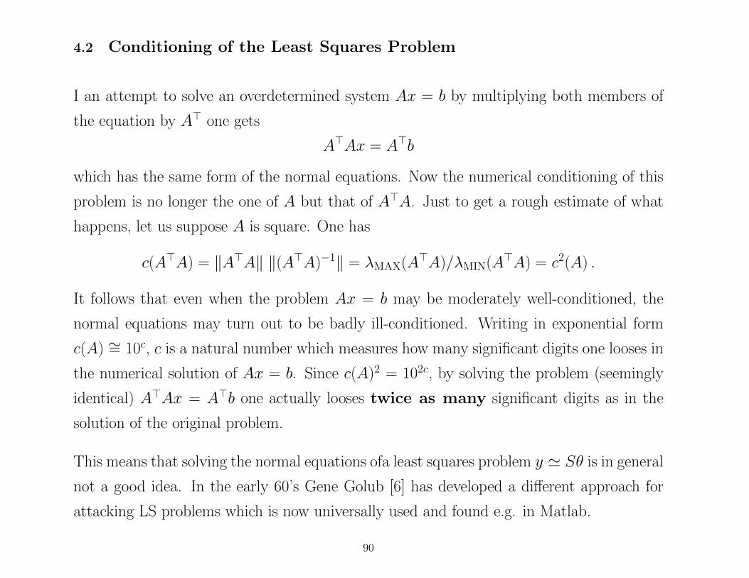
4.2 Conditioning of the Least Squares Problem
I an attempt to solve an overdetermined system Ax = b by multiplying both members of
the equation by A> one gets
A>Ax = A>b
which has the same form of the normal equations. Now the numerical conditioning of this
problem is no longer the one of A but that of A>A. Just to get a rough estimate of what
happens, let us suppose A is square. One has
c(A>A) = ‖A>A‖ ‖(A>A)−1‖ = λMAX(A>A)/λMIN(A>A) = c2(A) .
It follows that even when the problem Ax = b may be moderately well-conditioned, the
normal equations may turn out to be badly ill-conditioned. Writing in exponential form
c(A) ∼= 10c, c is a natural number which measures how many significant digits one looses in
the numerical solution of Ax = b. Since c(A)2 = 102c, by solving the problem (seemingly
identical) A>Ax = A>b one actually looses twice as many significant digits as in the
solution of the original problem.
This means that solving the normal equations ofa least squares problem y ' Sθ is in general
not a good idea. In the early 60’s Gene Golub [6] has developed a different approach for
attacking LS problems which is now universally used and found e.g. in Matlab.
90
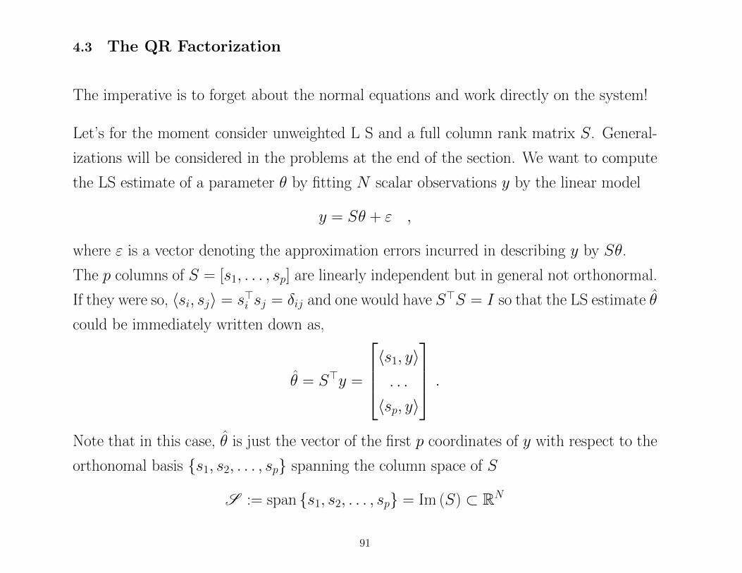
4.3 The QR Factorization
The imperative is to forget about the normal equations and work directly on the system!
Let’s for the moment consider unweighted L S and a full column rank matrix S. General-
izations will be considered in the problems at the end of the section. We want to compute
the LS estimate of a parameter θ by fitting N scalar observations y by the linear model
y = Sθ + ε ,
where ε is a vector denoting the approximation errors incurred in describing y by Sθ.
The p columns of S = [s1, . . . , sp] are linearly independent but in general not orthonormal.
If they were so, 〈si, sj〉 = s>i sj = δij and one would have S>S = I so that the LS estimate θ
could be immediately written down as,
θ = S>y =
〈s1, y〉. . .
〈sp, y〉
.
Note that in this case, θ is just the vector of the first p coordinates of y with respect to the
orthonomal basis s1, s2, . . . , sp spanning the column space of S
S := span s1, s2, . . . , sp = Im (S) ⊂ RN
91
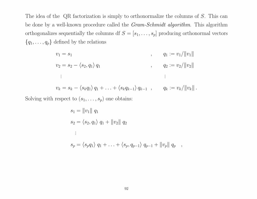
The idea of the QR factorization is simply to orthonormalize the columns of S. This can
be done by a well-known procedure called the Gram-Schmidt algorithm. This algorithm
orthogonalizes sequentially the columns df S = [s1, . . . , sp] producing orthonormal vectors
q1, . . . , qp defined by the relations
v1 = s1 , q1 := v1/‖v1‖
v2 = s2 − 〈s2, q1〉 q1 , q2 := v2/‖v2‖... ...
vk = sk − 〈skq1〉 q1 + . . . + 〈skqk−1〉 qk−1 , qk := vk/‖vk‖ .
Solving with respect to (s1, . . . , sp) one obtains:
s1 = ‖v1‖ q1
s2 = 〈s2, q1〉 q1 + ‖v2‖ q2
...
sp = 〈spq1〉 q1 + . . . + 〈sp, qp−1〉 qp−1 + ‖vp‖ qp ,
92
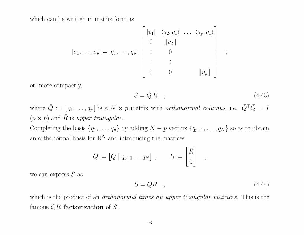
which can be written in matrix form as
[s1, . . . , sp] = [q1, . . . , qp]
‖v1‖ 〈s2, q1〉 . . . 〈sp, q1〉0 ‖v2‖... 0... ...
0 0 ‖vp‖
;
or, more compactly,
S = Q R , (4.43)
where Q := [ q1, . . . , qp ] is a N × p matrix with orthonormal columns; i.e. Q>Q = I
(p× p) and R is upper triangular.
Completing the basis q1, . . . , qp by adding N − p vectors qp+1, . . . , qN so as to obtain
an orthonormal basis for RN and introducing the matrices
Q :=[Q | qp+1 . . . qN
], R :=
[R
0
],
we can express S as
S = QR , (4.44)
which is the product of an orthonormal times an upper triangular matrices. This is the
famous QR factorization of S.
93
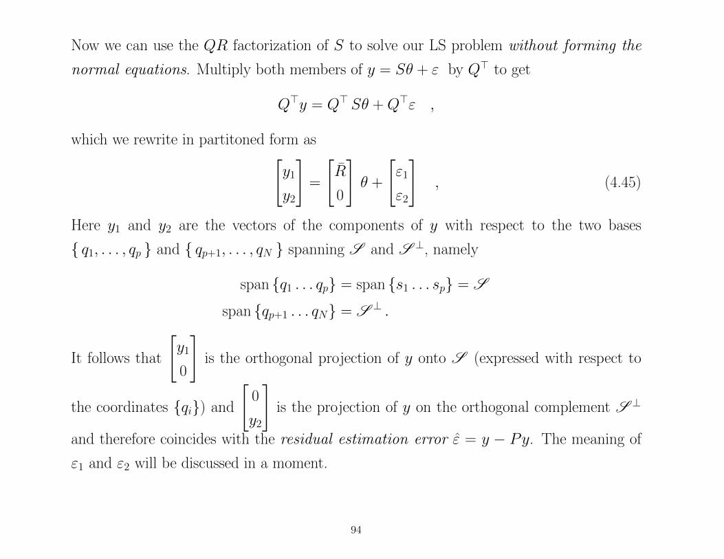
Now we can use the QR factorization of S to solve our LS problem without forming the
normal equations. Multiply both members of y = Sθ + ε by Q> to get
Q>y = Q> Sθ + Q>ε ,
which we rewrite in partitoned form as[y1
y2
]=
[R
0
]θ +
[ε1
ε2
], (4.45)
Here y1 and y2 are the vectors of the components of y with respect to the two bases
q1, . . . , qp and qp+1, . . . , qN spanning S and S ⊥, namely
span q1 . . . qp = span s1 . . . sp = S
span qp+1 . . . qN = S ⊥ .
It follows that
[y1
0
]is the orthogonal projection of y onto S (expressed with respect to
the coordinates qi) and
[0
y2
]is the projection of y on the orthogonal complement S ⊥
and therefore coincides with the residual estimation error ε = y − Py. The meaning of
ε1 and ε2 will be discussed in a moment.
94
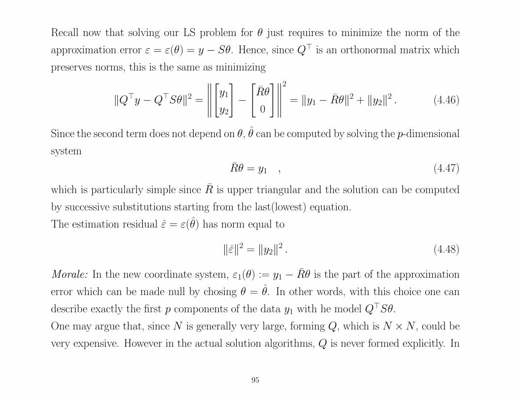
Recall now that solving our LS problem for θ just requires to minimize the norm of the
approximation error ε = ε(θ) = y − Sθ. Hence, since Q> is an orthonormal matrix which
preserves norms, this is the same as minimizing
‖Q>y −Q>Sθ‖2 =
∥∥∥∥∥[y1
y2
]−
[Rθ
0
]∥∥∥∥∥2
= ‖y1 − Rθ‖2 + ‖y2‖2 . (4.46)
Since the second term does not depend on θ, θ can be computed by solving the p-dimensional
system
Rθ = y1 , (4.47)
which is particularly simple since R is upper triangular and the solution can be computed
by successive substitutions starting from the last(lowest) equation.
The estimation residual ε = ε(θ) has norm equal to
‖ε‖2 = ‖y2‖2 . (4.48)
Morale: In the new coordinate system, ε1(θ) := y1 − Rθ is the part of the approximation
error which can be made null by chosing θ = θ. In other words, with this choice one can
describe exactly the first p components of the data y1 with he model Q>Sθ.
One may argue that, since N is generally very large, forming Q, which is N ×N , could be
very expensive. However in the actual solution algorithms, Q is never formed explicitly. In
95
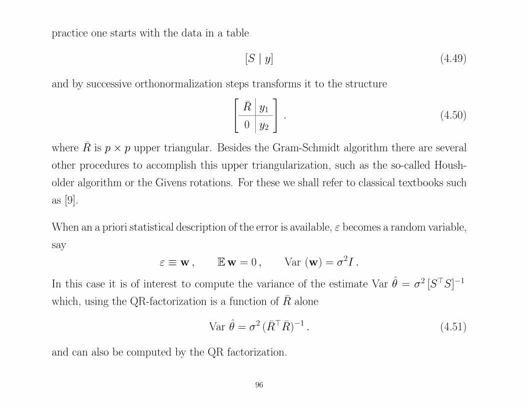
practice one starts with the data in a table
[S | y] (4.49)
and by successive orthonormalization steps transforms it to the structure[R y1
0 y2
]. (4.50)
where R is p× p upper triangular. Besides the Gram-Schmidt algorithm there are several
other procedures to accomplish this upper triangularization, such as the so-called Housh-
older algorithm or the Givens rotations. For these we shall refer to classical textbooks such
as [9].
When an a priori statistical description of the error is available, ε becomes a random variable,
say
ε ≡ w , Ew = 0 , Var (w) = σ2I .
In this case it is of interest to compute the variance of the estimate Var θ = σ2 [S>S]−1
which, using the QR-factorization is a function of R alone
Var θ = σ2 (R>R)−1 . (4.51)
and can also be computed by the QR factorization.
96
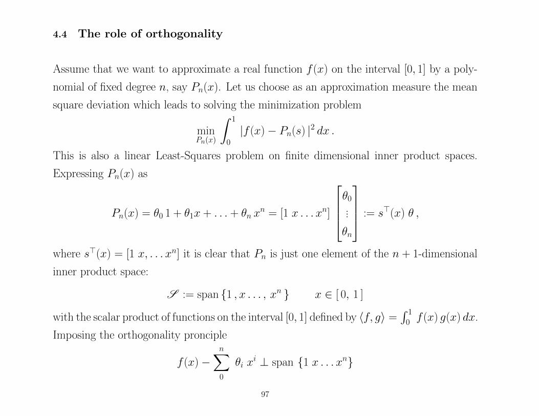
4.4 The role of orthogonality
Assume that we want to approximate a real function f (x) on the interval [0, 1] by a poly-
nomial of fixed degree n, say Pn(x). Let us choose as an approximation measure the mean
square deviation which leads to solving the minimization problem
minPn(x)
∫ 1
0
|f (x)− Pn(s) |2 dx .
This is also a linear Least-Squares problem on finite dimensional inner product spaces.
Expressing Pn(x) as
Pn(x) = θ0 1 + θ1x + . . . + θn xn = [1 x . . . xn]
θ0
...
θn
:= s>(x) θ ,
where s>(x) = [1 x, . . . xn] it is clear that Pn is just one element of the n + 1-dimensional
inner product space:
S := span 1 , x . . . , xn x ∈ [ 0, 1 ]
with the scalar product of functions on the interval [0, 1] defined by 〈f, g〉 =∫ 1
0 f (x) g(x) dx.
Imposing the orthogonality pronciple
f (x)−n∑0
θi xi ⊥ span 1 x . . . xn
97
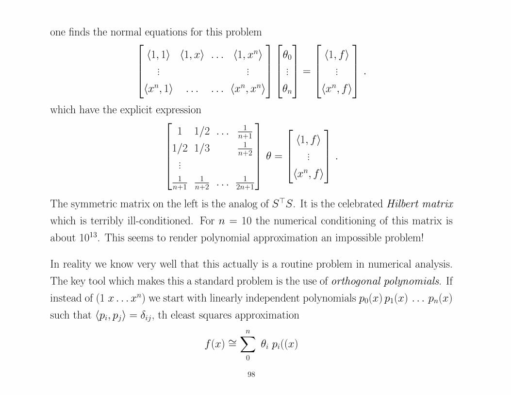
one finds the normal equations for this problem 〈1, 1〉 〈1, x〉 . . . 〈1, xn〉
... ...
〈xn, 1〉 . . . . . . 〈xn, xn〉
θ0
...
θn
=
〈1, f〉...
〈xn, f〉
.
which have the explicit expression1 1/2 . . . 1
n+1
1/2 1/3 1n+2
...1
n+11
n+2 . . . 12n+1
θ =
〈1, f〉...
〈xn, f〉
.
The symmetric matrix on the left is the analog of S>S. It is the celebrated Hilbert matrix
which is terribly ill-conditioned. For n = 10 the numerical conditioning of this matrix is
about 1013. This seems to render polynomial approximation an impossible problem!
In reality we know very well that this actually is a routine problem in numerical analysis.
The key tool which makes this a standard problem is the use of orthogonal polynomials. If
instead of (1 x . . . xn) we start with linearly independent polynomials p0(x) p1(x) . . . pn(x)
such that 〈pi, pj〉 = δij, th eleast squares approximation
f (x) ∼=n∑0
θi pi((x)
98
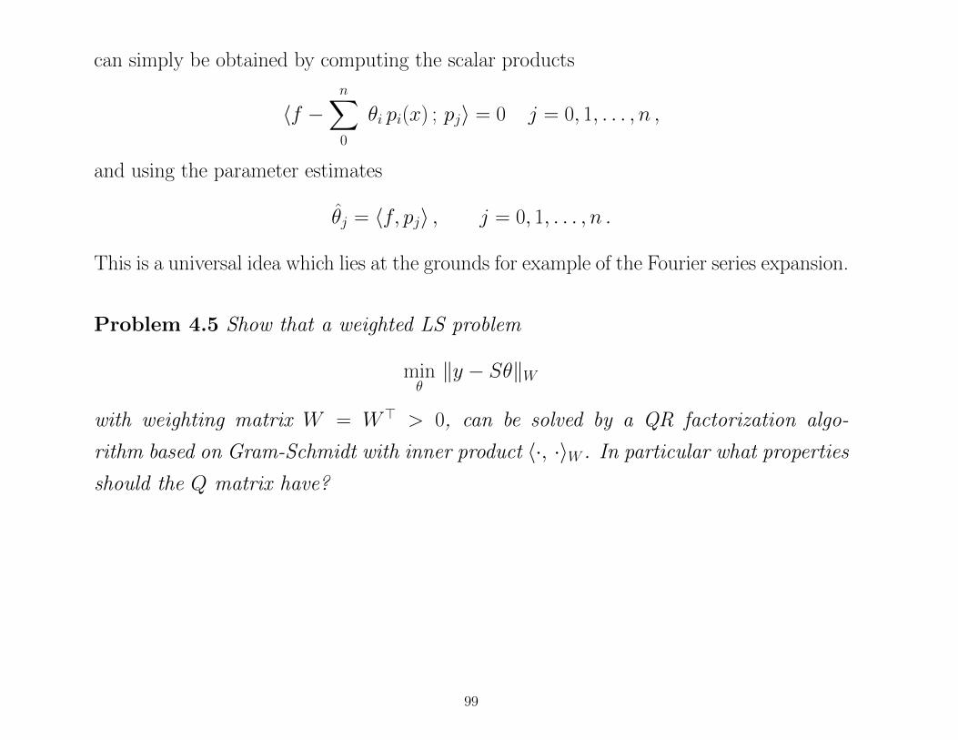
can simply be obtained by computing the scalar products
〈f −n∑0
θi pi(x) ; pj〉 = 0 j = 0, 1, . . . , n ,
and using the parameter estimates
θj = 〈f, pj〉 , j = 0, 1, . . . , n .
This is a universal idea which lies at the grounds for example of the Fourier series expansion.
Problem 4.5 Show that a weighted LS problem
minθ‖y − Sθ‖W
with weighting matrix W = W> > 0, can be solved by a QR factorization algo-
rithm based on Gram-Schmidt with inner product 〈·, ·〉W . In particular what properties
should the Q matrix have?
99
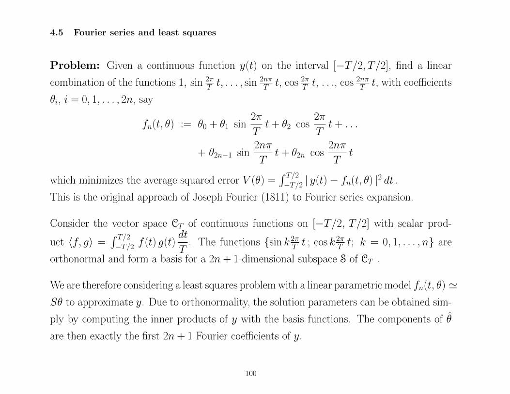
4.5 Fourier series and least squares
Problem: Given a continuous function y(t) on the interval [−T/2, T/2], find a linear
combination of the functions 1, sin 2πT t, . . . , sin
2nπT t, cos 2π
T t, . . ., cos 2nπT t, with coefficients
θi, i = 0, 1, . . . , 2n, say
fn(t, θ) := θ0 + θ1 sin2π
Tt + θ2 cos
2π
Tt + . . .
+ θ2n−1 sin2nπ
Tt + θ2n cos
2nπ
Tt
which minimizes the average squared error V (θ) =∫ T/2−T/2 | y(t)− fn(t, θ) |2 dt .
This is the original approach of Joseph Fourier (1811) to Fourier series expansion.
Consider the vector space CT of continuous functions on [−T/2, T/2] with scalar prod-
uct 〈f, g〉 =∫ T/2−T/2 f (t) g(t)
dt
T. The functions sin k 2π
T t ; cos k 2πT t; k = 0, 1, . . . , n are
orthonormal and form a basis for a 2n + 1-dimensional subspace S of CT .
We are therefore considering a least squares problem with a linear parametric model fn(t, θ) 'Sθ to approximate y. Due to orthonormality, the solution parameters can be obtained sim-
ply by computing the inner products of y with the basis functions. The components of θ
are then exactly the first 2n + 1 Fourier coefficients of y.
100
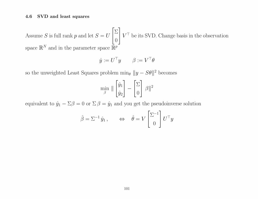
4.6 SVD and least squares
Assume S is full rank p and let S = U
[Σ
0
]V > be its SVD. Change basis in the observation
space RN and in the parameter space Rp
y := U>y β := V >θ
so the unweighted Least Squares problem minθ ‖y − Sθ‖2 becomes
minβ‖
[y1
y2
]−
[Σ
0
]β‖2
equivalent to y1 − Σβ = 0 or Σ β = y1 and you get the pseudoinverse solution
β = Σ−1 y1 , ⇔ θ = V
[Σ−1
0
]U>y
101
5 INTRODUCTION TO INVERSE PROBLEMS
Problem of recovering Input/cause from output/effect e.g. recovering forces acting on an
object from its motion (Newton)
Image deconvolution (deblurring)
Recovering initial conditions from given solutions to ODE or PDE
System identification: recovering the differential equation from (measurements of) a solution
These problems require an operator inversion. Most elementary example Ax = b
1. Given A, x compute b = Ax (Direct problem)
2. Given A and b recover x (Inverse problem)
Inverse problems are sensitive to perturbations. For the Ax = b problem this sensitivity
is captured by the notion of ill-conditioning. Need a more general concept for physical
problems where A is an operator acting on functions and x and b may be functions (but b
may be a discretization of an observed function).
102
5.1 Ill-posed problems
The problem
Ax = y; x ∈ X, y ∈ Y; A : X→ Y
is said to be well-posed in the sense of Hadamard if the following conditions hold:
1. For each y ∈ Y there exists x ∈ X, such that Ax = y (existence)
2. For each y ∈ Y there exists a unique x ∈ X, such that Ax = y (uniqueness)
3. The solution depends continuously on the data y
Example of ill-posed problems:
Recover a continuous function f (t) from its sample values f (tk); k = 1, 2, . . ..Recover the derivative of a function f (t) from its sample values f (tk); k = 1, 2, . . ..Solve an integral equation
y(t) =
∫T
k(t− s)x(s)ds
possibly from sample values y(tk); k = 1, 2, . . ..
103
5.2 From ill-posed to ill-conditioned
In practice all problems need to be solved by discretization. Transform Ax = y into Ax = b.
If the original problem was ill-posed then the discretized one is normally ill-conditioned.
The solution need not exist and the effect of small perturbations on b can be large variations
of x. The problem is “relaxed” to an optimization problem: Typically least squares:
minx‖y − Ax‖
yet the solution can still be very wild. Random perturbations on y are amplified by
ill-conditioning. Want to constrain the solution to be smooth !
Regularization: Assume X, Y are inner product spaces (finite dimensional)
minx‖y − Ax‖Y + λ‖x‖X , λ ≥ 0
The norm ‖x‖X is arbitrary; weights large variations. Example ‖x‖2X =
∑t x(t)2 (`2 norm).
104
5.3 Regularized Least Squares problems
Assume X, Y are finite dimensional inner product spaces with
〈ξ, η〉Y = ξ>Qη 〈ξ, η〉X = ξ>Wη ,
where Q and W are positive definite.
Theorem 5.1 The solution of the regularized least squares problem is
x =[A>QA + λW
]−1A>Qy (5.52)
When λ→ 0
limλ→0
[A>QA + λW
]−1A>Q = A†
(the Moore-Penrose pseudoinverse).
Will see later a proof and the interpretation in terms of linear Bayesian estimation.
105
6 Vector spaces of second order random variables (1)
Random variables x ≡ x(ω) defined in the same experiment (probability space) Ω, Pwhich have finite second moment, E |x|2 < ∞, are called second order random vari-
ables. Recall that the expectation of a random variable is the mean value over all possible
“experimental conditions” ω
Ex =∑ωk
x(ωk)P (ωk) ≡∫
Ω
x(ω) dP =
∫Rx dFx(x)
The set of real or complex-valued second-order random variables x defined on the same
probability space is a vector space under the usual operations of sum and multiplication
by real (or complex) numbers. This vector space comes naturally equipped with an inner
product
〈x,y〉 := Exy =
∫Ω
x(ω)y(ω) dP (6.53)
which is just the correlation of the random variables x, y. The norm ‖x‖ = 〈x,x〉1/2
induced by this inner product (the square root of the second moment of x) is positive, i.e.
‖x‖ = 0⇔ x = 0, if we agree to identify random variables which are equal almost surely,
i.e. differ on a set of probability zero. The set of second-order random variables x, equipped
with the inner product 〈·, ·〉, is an inner product (Hilbert) space.
106
6.1 Vector spaces of second order random variables (2)
To simplify notations it is convenient to subtract off the expected value. From now consider
only zero mean second-order random variables x := x−Ex describes random fluctuations
about the “mean value” Ex. The covariance of x,y is 〈x, y〉 = E xy, denoted σx,y.
Problem 6.1 Show that m scalar (zero-mean) second order random variables x1, . . . ,xm
are linearly independent if and only if their Covariance matrix Σx = [ σxixj ]i,j=1,m =
[Exixj ]i,j=1,m is non-singular (i.e. positive definite) (note: Σx is the Gramian
of x1, . . . ,xm).
Vector notation: let x> :=[x1 . . . xm
]then Σx := Exx> .
If Σx > 0 the space
H(x) =
m∑k=1
αk xk ; αk ∈ R
is an m-dimensional real inner product space. Notation: H(x) = span x1, . . . ,xm.
107
6.2 About “random vectors”
Often it is useful to organize n-tuples of random variables as n×1 matrices (column vectors),
say
y =
y1
y2
...
yn
These objects are usually called “random vectors” but the correct denomination should
probably be be “vector-valued random variables”. Gaussian random vectors have a proba-
bility density function depending only on the mean vector µ and the Covariance matrix Σ:
p(ξ1, . . . , ξn) =1
[ 2πn det Σ]1/2exp−1
2
[ξ1 − µ1 . . . ξn − µn
]Σ−1
ξ1 − µ1
. . .
ξn − µn
Uniquely determined by the parameters µ, Σ.
108
6.3 Sequences of second order random variables
A random signal is just a sequence (possibly infinite) of zero-mean random variables
indexed by time
y := y(1), . . . ,y(t), . . . ,y(N) , N ≤ +∞
The y(t) maybe vector valued; but we shall only consider scalar R-valued variables. Write
y as a column vector.
Let α ∈ RN be a deterministic sequence ; the linear functions of y
z = α>y =
N∑t=1
α(t)y(t)
are just the elements of the subspace linearly generated by the random variables y(t) :
H(y) := span y(t) | t = 1, . . . , N ≡ α>y ; α ∈ RN
Assume that y(1), . . . ,y(t), . . . ,y(N) are linearly independent (a basis), then the coordi-
nates α(1), . . . , α(N) of each z are unique;
the covariance matrix Σy is non singular and the space H(y) is an N -dimensional real inner
product space. Denote
z =
N∑k=1
α(k) y(k) := α>y , w =
N∑k=1
β(k) y(k) := β>y ,
109
then we have
〈z, w〉 = E zw =∑k
∑j
αkE (ykyj)βj = α>Σyβ
Hence H(y) is isometrically isomorphic to the weighted inner product space (RN , 〈·, ·〉Σy ).
Note: Although random vectors y of the same dimension form a (real or complex) vector
space, linear operations on families of these objects (vector-valued signals) are not useful in
applications since making linear combinations by scalar multipliers, all scalar components of
each vector y(t) are treated in the same way. One should rather define linear combinations
by matrix multipliers say
z = A1y(1) + A1y(2) + . . . + ANy(N) , Ak ∈ Rn×n
as it was originally attempted in the literature (Wiener-Masani 1955). The resulting struc-
ture is however no longer a vectorspace but a module, called Rn×n-module which is more
complicated to deal with than vector spaces. For us the “vectors” will always be scalar
random variables.
110
6.4 Principal Components Analysis (PCA)
Probabilistic analog of Fourier series expansion. The sin and cos functions are generalized
to orthonormal sequences and the Fourier coefficients are random. The procedure can be
generalized to infinite sequences (stochastic processes) and takes a different name; it is called
the Kahrunen-Loeve expansion.
Problem 6.2 Express the random signal y as a linear combination of n deterministic
modes ϕk (orthonormal sequences in RN) weighted by uncorrelated random coefficients.
y(t) =∑k
xkϕk(t) t = 1, 2, . . . , N
1. The deterministic vectors ϕk are orthonormal in RN
2. The xk form an orthogonal basis in H(y)
111
Let ϕk be the k-th normalized eigenvector of Σy correspond to the (positive) eigenvalue λ2k
Σyϕk = λ2k ϕk , k = 1, 2, . . . , N
then define random variables xk = ϕ>k y. These are uncorrelated:
Exkxj = Eϕ>k yϕ>j y = ϕ>k E [y y>]ϕj = λ2k δk,j
Can make xk into an orthonormal basis for H(y) by
xk :=1
λkϕ>k y
so that
y =
N∑k=1
〈y, xk〉 xk =
N∑k=1
E [y y>]1
λkϕk xk =
N∑k=1
Σy1
λkϕk xk =
=
N∑k=1
xk ϕk
The random signal y is a linear combination of N deterministic modes ϕk (orthonormal
in RN) weighted by uncorrelated random coefficients.
112
Each component has expected “energy”
E∑t
(xk ϕk(t))2 = E (x2
k)ϕ>k ϕk = λ2
k
If we arrange the eigenvalues in decreasing magnitude so that
‖x1‖2 = λ21 ≥ . . . ≥ ‖xN‖2 = λ2
N
then the first component x1 ϕ1 has maximum energy while the others have decreasing
energy with k. If the first k eigenvalues λ1, . . . , λk are much bigger than the others can
approximate the signal with the first k modes. These are the Principal Components
of the signal.
The expansion y(t) =∑N
k=1 xk ϕk(t) can be interpreted as a generalization of the Fourier
expansion of a random signal with ϕ1, . . . , ϕN generalizing the sin− cos functions and xk
being the related Fourier coefficients. This follows from xk = ϕ>k y which is interpreted as
a discrete integral
xk =
N∑k=1
ϕk(t)y(t)
113
6.5 Bayesian Least Squares Estimation
Consider a “static” finite-dimensional estimation problem where the observable y is a ran-
dom vector with m components and x is an n-dimensional inaccessible random vector of
dimension n. Assume that the joint covariance matrix of x and y is known:
Σ =
[Σx Σxy
Σyx Σy
]
Definition 6.1 The best linear estimator of x based on (or given) y, is the n-dimensional
random vector x, whose components xk ∈ H(y), k = 1, . . . , n, individually solve the
minimum problems
xk = arg minzk∈H(y)
‖xk − zk‖ k = 1, . . . , n, (6.54)
Clearly the n scalar optimization problems (6.54) can be reformulated as one single equiv-
alent problem where one seeks to minimize
var (x− z) :=
n∑k=1
‖xk − zk‖2, zk ∈ H(y)
which is the scalar variance of the error vector x− z. The scalar variance is the trace of
the matrix
Var (x− z) := E (x− z)(x− z)>.
114
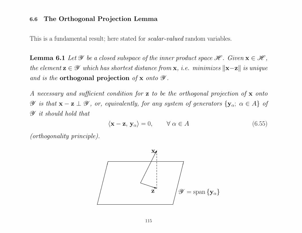
6.6 The Orthogonal Projection Lemma
This is a fundamental result; here stated for scalar-valued random variables.
Lemma 6.1 Let Y be a closed subspace of the inner product space H . Given x ∈H ,
the element z ∈ Y which has shortest distance from x, i.e. minimizes ‖x−z‖ is unique
and is the orthogonal projection of x onto Y .
A necessary and sufficient condition for z to be the orthogonal projection of x onto
Y is that x − z ⊥ Y , or, equivalently, for any system of generators yα; α ∈ A of
Y it should hold that
〈x− z, yα〉 = 0, ∀ α ∈ A (6.55)
(orthogonality principle).
x
Y = span yα
PPPPPqz
115
In view of Lemma 6.1, xk is the orthogonal projection of xk onto H(y). Notation:
xk = E [ xk | H(y) ] (6.56)
The notation E [ x | H(y)] will be used also when x is vector-valued. The symbol denotes
the vector with components E [ xk | H(y)] , k = 1, . . . n.
When the projection is expressed in terms of some specific set of generators say y = yα(i.e. H(y) = span yα), we shall denote it E [ x | y ].
Problem 6.3 Let x be a scalar random variable. If yα ≡ e1, . . . , em is an or-
thonormal basis in Y then:
x = E [ x | H(y) ] =
m∑k=1
〈x, ek〉 ek =
m∑k=1
E (x, ek) ek
The formula holds also when x is a random vector.
Note that the projection is a linear function of the vector e = [ e1, . . . , em]> generating the
space of observations.
When the components of y are not orthonormal the formula is a bit more complicated.
116
Theorem 6.1 Let x and y be zero-mean second-order random vectors of dimensions
n and m respectively with covariance matrix (6.5). Then the orthogonal projection
(minimum variance linear estimator) of x onto the linear subspace spanned by the
components of y is given by
E [ x | y ] = Σxy Σ−1y y (6.57)
When Σy is singular the inverse is replaced by the Moore-Penrose pseudoinverse (see
Sect. 3.6).
The (residual) error vector has covariance matrix,
Λ := Var (x− E [ x | y]) = Σx − Σxy Σ−1y Σyx. (6.58)
This is the smallest error covariance matrix obtainable in the class of all linear func-
tions of the data, i.e. Λ ≤ Var (x−Ay) for any matrix A ∈ Rn×m, where the inequality
is understood in the sense of the positive semidefinite ordering among symmetric ma-
trices.
Proof: Writing the vector z as z = Ay, and invoking the orthogonality condition (6.55) for
each component xk, we obtain
E (x− Ay)y> = 0 (n×m)
117
which is equivalent to Σxy−AΣy = 0. If Σy is non-singular (6.57) is proven. The case when
Σy is singular is discussed in the Section on pseudo inverse.
The formula for the error covariance follows from the orthogonality condition
E (x− Σxy Σ−1y y)(x− Σxy Σ−1
y y)> = E (x− Σxy Σ−1y y)x>
since the components of the error x := x − Σxy Σ−1y y must be orthogonal to any linear
function of the vector y.
For what concerns the minimum matrix variance property of the estimator, we see that for
arbitrary A ∈ Rn×m, one has
Var (x− Ay) = Var (x− E [ x | y] + E [ x | y]− Ay) = Λ + Var (E [ x | y]− Ay)
as E [x | y] − Ay has components in H(y) and hence is (componentwise) orthogonal to
x−E [ x | y]. On the other hand the matrix Λ does not depend on A while the second term
in the sum can be made zero for Ay = E [ x | y]. Hence the minimum property follows
and this concludes the proof of Theorem 6.1.
118
6.7 Block-diagonalization of Symmetric Positive Definite matrices
The estimation error x := x − E [ x | y] is orthogonal to y; hence Var
[y
x
] is block-
diagonal
Var
[y
x
] =
[Σy 0
0 Λ
], Λ = Σx − Σxy Σ−1
y Σyx.
In matrix language the block Λ is called the Schur Complement of Σy in Σ. The order
here is immaterial; can exchange x with y.
Generalization. Let
X =
[A B>
B D
]∈ R(n+m)×(n+m)
be symmetric positive definite (a covariance matrix). If A is invertible, then[I 0
−BA−1 I
]X
[I −A−1B>
0 I
]=
[A 0
0 D −BA−1B>
]Proof via Bayesian Estimation Theory. Think of A as Σy, D as Σx and B as Σxy.
So that,
1. X is positive definite if and only if A and S := D −BA−1B> are positive definite.
2. If A is invertible, X is positive semi-definite if and only if A is positive definite and
S := D −BA−1B> is positive semi-definite.
119
Problem 6.4 Show, only assuming X symmetric, that,
1. X is positive definite if and only if D and S := A−BD−1B> are positive definite.
2. If D is invertible, X is positive semi-definite if and only if D is positive definite
and S := S := A−B>D−1B is positive semi-definite.
Can generalize the bock-diagonalization formulas to non-necessarily symmetric nor positive
definite matrices. Consider a square block matrix
X =
[A B
C D
]∈ R(n+m)×(n+m)
Definition 6.2 Assume that A is non-singular. The matrix S1 := D − CA−1B is
called Schur complement of A in X.
Assume that D is non-singular. The matrix S2 := A−BD−1C is called Schur comple-
ment of D in X.
Proposition 6.1 Assume that A is invertible. Then X is invertible if and only if
also the Schur complement D − CA−1B is invertible.
Dually, if D is invertible X is invertible if and only if also the Schur complement
A−BD−1C is invertible.
120
Proof: If A is non-singular, we have,
X
[I −A−1B
0 I
]=
[A B
C D
][I −A−1B
0 I
]=
[A 0
C D − CA−1B
][
I 0
−CA−1 I
][A 0
C D − CA−1B
]=
[A 0
0 D − CA−1B
]so that [
I 0
−CA−1 I
]X
[I −A−1B
0 I
]=
[A 0
0 D − CA−1B
]and the first statement follows since the two block-triangular matrices are both invertible.
Then, if A and D − CA−1B are non-singular,
X−1 =
[I −A−1B
0 I
][A 0
0 D − CA−1B
]−1 [I 0
−CA−1 I
]or
X−1 =
[I −A−1B
0 I
][A−1 0
0 (D − CA−1B)−1
][I 0
−CA−1 I
]or
X−1 =
[A−1 + A−1B(D − CA−1B)−1CA−1 −A−1B(D − CA−1B)−1
−(D − CA−1B)−1CA−1 (D − CA−1B)−1
]
121
6.8 The Matrix Inversion Lemma (ABCD Lemma)
Problem 6.5 Show that if D, and A−BD−1C are non-singular, then
X−1 =
[(A−BD−1C)−1 −(A−BD−1C)−1BD−1
−D−1C(A−BD−1C)−1 D−1 + D−1C(A−BD−1C)−1BD−1
]
By comparison we have the famous Sherman - Morrison - Woodbury matrix inversion
formula: If A, D, and one of the Schur complements (A − BD−1C) and (D − CA−1B)
are non-singular, then the other Schur complement is non-singular and
(A + BD−1C)−1 = A−1 − A−1B(D + CA−1B)−1CA−1
This formula is useful when the“perturbation” BD−1C of A has low rank, in particular
when D is a scalar (1× 1) matrix. It is used for example in recursive least squares and in
Kalman filtering.
Problem 6.6 Let
X =
[A B
B> D
]∈ R(n+m)×(n+m)
be symmetric. Prove that X is positive semi-definite if and only if D ≥ 0, kerD ⊆kerB and the generalized Schur complement S := A−BD+B> is positive semidefinite.
122
6.9 Change of basis
Assume that the m components of y = [ y1, . . . ,ym ]> are linearly independent and let
z1, . . . , zm be m other linearly independent random variables (a new basis) in H(y) so
that H(z) = H(y) .
Clearly z = Ty for some non-singular T ∈ Rm×m since by equality of the two vector spaces
we have y = Sz, for some S ∈ Rm×m so that y = STy, and Σy = ST Σy which implies
ST = I . Hence
Σzy = T Σy ; T = Σzy Σ−1y
that is z = E (z | y) and z coincides with its orthogonal projection onto H(y).
Problem 6.7 Let x be an arbitrary random vector in H; how does E (x | y) = Ay
changes under a change of basis z = Ty ?
Hint use: Σz = T Σy T> .
In particular if we want to change y to an orthonormal basis e :=[e1 e2 . . . em
]>need to find T such that
I = T Σy T> .
123
6.10 Cholesky Factorization
Finding T such that I = T Σy T> is the same as finding (invertible) S ∈ Rm×m such that
SS> = Σy and then T = S−1. There are many such square roots of Σy.
Theorem 6.2 Let Q = Q> be positive definite. There is a unique lower triangular
matrix L, with positive diagonal elements such that Q = LL>. This factor can be
computed by the following algorithm which works sequentially starting from the upper
left element `1,1 :=√q11 descending and working from left to right.
1. The diagonal elements `ii are computed by
`ii =
√√√√qii −i−1∑j=1
`2ij i = 1, . . . , n . (6.59)
2. Assuming the first i−1 rows of L have been computed, the elements of the following
i-th row are given by
`ij =1
`jj
(qij −
j−1∑k=1
`ik `jk
)j = 1, . . . , i− 1 (j < i) . (6.60)
This equation requires the elements of the i-th row `i1, . . . , `i,j−1 and the previous
elements `j1, . . . , `j,j−1 of the j-th row which are all known since the j-th row lies
above the i-th.
124
Proof. By induction on the dimension k of Q. Let
Qk+1 =
[Qk r
r> q
]∈ R(k+1)×(k+1)
symmetric and positive definite. Then a factorization Qk+1 = Lk+1L>k+1 can hold with
lower triangular factors of the form :
Lk+1 =
[Lk 0
`> λ
]L>k+1 =
[L>k `
0 λ
]if and only if
Lk L>k = Qk
Lk ` = r
`>` + λ2 = q .
the first of which is true by the inductive hypothesis since Qk is symmetric and positive
definite. the second equation yields ` = L−1k r which substituted into the third yields a
unique positive solution λ, since the difference
q − `>` = q − r>(L>k )−1 L−1k r = q − r>Q−1
k r
is the positive Schur complement of Qk. In fact
q − r>Q−1k r = [r>Q−1
k − 1]
[Qk r
r> q
][Q−1k r
−1
]≥ 0 .
125
6.11 Bayesian estimation for a linear model
Often the relation between the observations y and the unknown random vector x can be
described by a linear relation
y = Sx + w (6.61)
where S ∈ RN×n is a known matrix, x and w are zero-mean uncorrelated random vectors of
respective variance matrices, P := Var (x) and R := Var (w) which we assume known. The
model represents a quite general prototype of measurements affected by random additive
errors or noise. We want to find an expression for the linear Bayesian estimate E [x | y] of
x given y.
In order to apply formula (??); first need to compute the matrices Σxy and Σy. Since x
and w are orthogonal,
Σyx = S Σx = SP ⇒ Σxy = PS> and, Σy = SPS> + R (6.62)
Assume Σy > 0, which is certainly true if R > 0, then
E[x | y] = PS>(SPS> + R)−1 y . (6.63)
and the variance matrix Λ, of the estimation error x = x− E[x | y]
Λ = P − PS>(SPS> + R)−1 SP . (6.64)
126
6.12 Use of the Matrix Inversion Lemma
Easier to use expression for the estimator when for example R is a diagonal matrix.
Theorem 6.3 Assume that the a priori variance matrix P of x is invertibile. Then
E[x | y] = (S>R−1S + P−1)−1 S>R−1 y;
Λ = (S>R−1S + P−1)−1 . (6.65)
Proof. Use the Matrix Inversion Lemma (??) with A = P−1, B = S>, C = R−1. and
E(x | y) = PS>[R−1 −R−1 S(S>R−1S + P−1)−1 S>R−1
]y
=[P − PS>R−1 S(S>R−1S + P−1)−1
]S>R−1y
=[P (S>R−1 S + P−1)− PS>R−1S
](S>R−1S + P−1)−1 S>R−1 y
check that the term within square brackets is the identity.
127
6.13 Interpretation as a regularized least squares
Compare with the formulas for the regularized Least Squares of Theorem 5.1. The formula
for the estimator in (6.65) is the same as (5.52) provided we interpret Q and W as R−1 and
P−1 respectively.
TBA
128
6.14 Application to Canonical Correlation Analysis (CCA)
Canonical Correlation Analysis is a useful tool in many statistical applications. It is for
example used in model reduction and in system identification. Assume you have two fam-
ilies of second order zero-mean real random variables written as vectors, say x and y of
dimensions n and m. We want to know which of the (output) components yj is “most
influenced” by what (input) component, say xk, of x. Actually, as stated, this question
turns out to have no precise answer.
Let the finite-dimensional subspaces X , Y
X ≡ H(x) = span x1, . . . ,xn Y ≡ H(y) = span y1, . . . ,ym
be endowed with the usual inner product 〈ξ,η〉 = E ξη. The dimensions of H(x), H(y)
are exactly n and m if and only if the covariance matrices
Σx = E xx>, Σy = E yy>
are positive definite. In this case H(x), H(y) are isomorphic, respectively, to Rn with
inner product 〈·, ·〉Σx and to Rm with inner product 〈·, ·〉Σy. We shall instead consider the
following
129
Problem: Find two orthonormal bases, v := v1, . . . ,vn for H(x) and u := u1, . . . ,umfor H(y), such that
E vj uk = σk δj,k, j = 1, . . . , n, k = 1, . . . ,m . (6.66)
so that vj may have a non-zero correlation only with a corresponding variable uj
having the same index.
Note that the variables are normalized to unit variance so the correlation is not influenced
by the“power” of the random variables which are being compared.
Note: (6.66) is the same as requiring that the covariance matrix of the two random vectors
v := [v1, . . . ,vn]> and u := [u1, . . . ,um]> should be diagonal; i.e.,
E uv> =
σ1 0 . . . 0 . . . 0
0 σ2 . . . 0 . . . 0... . . . . . . ...
0 σr . . . 0
0 0 . . . 0 . . . 0
, r ≤ min(n,m)
where we want σ1, σ2, . . . , σr to be positive and ordered in decreasing magnitude.
Fact: all σk’s are less or equal to one since the random variables vj uk have unit variance
(norm). In fact, say, σ1 = 1 if and only if u1 and v1 are parallel and hence coincide.
130
Problem 6.8 Show that all σk’s are less or equal to one and can be equal to one only
when the spaces H(x) and H(y) have a non zero intersection.
We shall show that the special bases v and u satisfying (6.66) are essentially unique and
can be constructed by a SVD of a certain map. They are called the bases of canonical
variables in H(x) and H(y) respectively and the numbers σk are called the canonical
correlation coefficiens.
Since σk ≤ 1 , ; k = 1, . . . , r we can also define canonical (or principal) angles, θk,
between the subspaces H(x) and H(y) by setting
cos θk := σk , ; k = 1, . . . , r
We have σ1 < 1 if and and only if the (first canonical) angle between H(x) and H(y) is
positive, which is equivalent to H(x) ∩H(y) = 0.
Consider now the orthogonal projection operator (6.56); i.e. E [ · | H(y)] : H(x) → H(y)
Problem 6.9 Show that the adjoint of this map is the orthogonal projection
E [ · | H(x)] : H(y) → H(x) .
131
By the defining properties of the canonical variables one should have
E [vj | H(y) ] = E [vj | u] = σjuj, j = 1, 2, . . . ,m,
E [uk | H(x) ] = E [uk | v] = σkvk, k = 1, 2, . . . , n (6.67)
where some of the last canonical correlation coefficients may be zero. These relations are
to be compared with (3.29).
Proposition 6.2 Canonical correlation analysis of the spaces H(x) and H(y) is ac-
complished by SVD of the Orthogonal Projection operator E [ · | H(y)] in the sense
that if 1
E [ · | H(y)] =
n∑i=1
σi ui 〈vi, · 〉 ,
is the SVD of E [ · | H(y)] then the nonzero singular values σi ; i = 1, . . . , r are
the canonical correlation coefficients and ui vi ; i = 1 ; . . . , n are the corresponding
canonical variables.
We want to do Canonical Correlation Analysis by the usual matrix SVD. To this end we
need a matrix representation of this operator.
For an arbitrary ξ = a>x ∈ H(x),
E [ ξ | H(y)] = a>E x y>Σ−1y y, Σy := E yy>.
1Assume w.l.o.g. that m ≥ n. Then the variables vi ; i > n in the expression are understood to be zero.
132
So in the original bases the representation of E [ · | H(y)] is matrix multiplication (from
the right)
a> → a>E xy>Σ−1y = a>ΣxyΣ−1
y
A Warning : Note that in order to express the inner product of random elements in
H(x), H(y) in terms of their coordinates, we must introduce appropriate weights to form
the inner products in the coordinate spaces. In fact, the inner product of two elements
ξi = a>i x ∈ H(x), i = 1, 2, induces on Rn the inner product
〈a1, a2〉Σx := a>1 Σx a2, Σx := E xx>.
Similarily, the inner product corresponding to the basis y for H(y) is 〈b1, b2〉Σy := b>1 Σy b2.
Hence, the matricial SVD needs to be done in the weighted inner product
spaces !
To obtain the usual Euclidean inner product in Rn, the bases need to be orthonor-
mal !. Only in this case the matrix representation of the adjoint of E [· | H(y)] is the
transpose of its matrix representation.
133
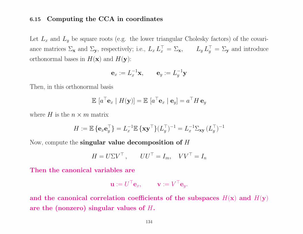
6.15 Computing the CCA in coordinates
Let Lx and Ly be square roots (e.g. the lower triangular Cholesky factors) of the covari-
ance matrices Σx and Σy, respectively; i.e., LxL>x = Σx, Ly L
>y = Σy and introduce
orthonormal bases in H(x) and H(y):
ex := L−1x x, ey := L−1
y y
Then, in this orthonormal basis
E [a>ex | H(y)] = E [a>ex | ey] = a>H ey
where H is the n×m matrix
H := E exe>y = L−1x E xy>(L>y )−1 = L−1
x Σxy (L>y )−1
Now, compute the singular value decomposition of H
H = UΣV > , UU> = Im, V V > = In
Then the canonical variables are
u := U>ex, v := V >ey.
and the canonical correlation coefficients of the subspaces H(x) and H(y)
are the (nonzero) singular values of H.
134
7 KRONECKER PRODUCTS
To answer the question: How do linear maps between vector spaces of matrices (Rm×n or
Cm×n) look like?
Motivation: Need to solve MATRIX EQUATIONS.
Consider the Lyapunov equations:
AX + XA> = Q, X − AXA> = Q
When do these equations admit solutions? We know that a solution exists and is unique if
A is stable (in the continuos-time and discrete-time sense). What if A is not stable? what
about the following more general linear matrix equations ?
AX + XB = Q, X − AXB = Q
The Kronecker product is a powerful tool to study this and many other applications (not
just Systems and Control, also to Physics).
135
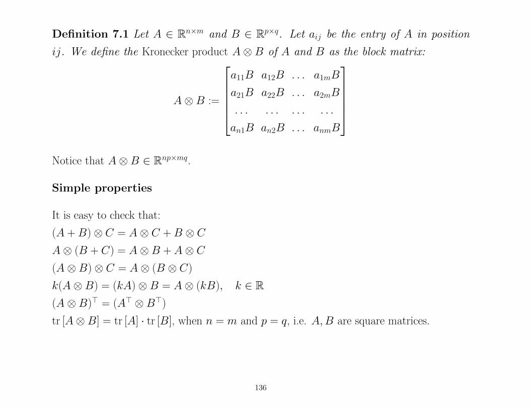
Definition 7.1 Let A ∈ Rn×m and B ∈ Rp×q. Let aij be the entry of A in position
ij. We define the Kronecker product A⊗B of A and B as the block matrix:
A⊗B :=
a11B a12B . . . a1mB
a21B a22B . . . a2mB
. . . . . . . . . . . .
an1B an2B . . . anmB
Notice that A⊗B ∈ Rnp×mq.
Simple properties
It is easy to check that:
(A + B)⊗ C = A⊗ C + B ⊗ CA⊗ (B + C) = A⊗B + A⊗ C(A⊗B)⊗ C = A⊗ (B ⊗ C)
k(A⊗B) = (kA)⊗B = A⊗ (kB), k ∈ R(A⊗B)> = (A> ⊗B>)
tr [A⊗B] = tr [A] · tr [B], when n = m and p = q, i.e. A,B are square matrices.
136
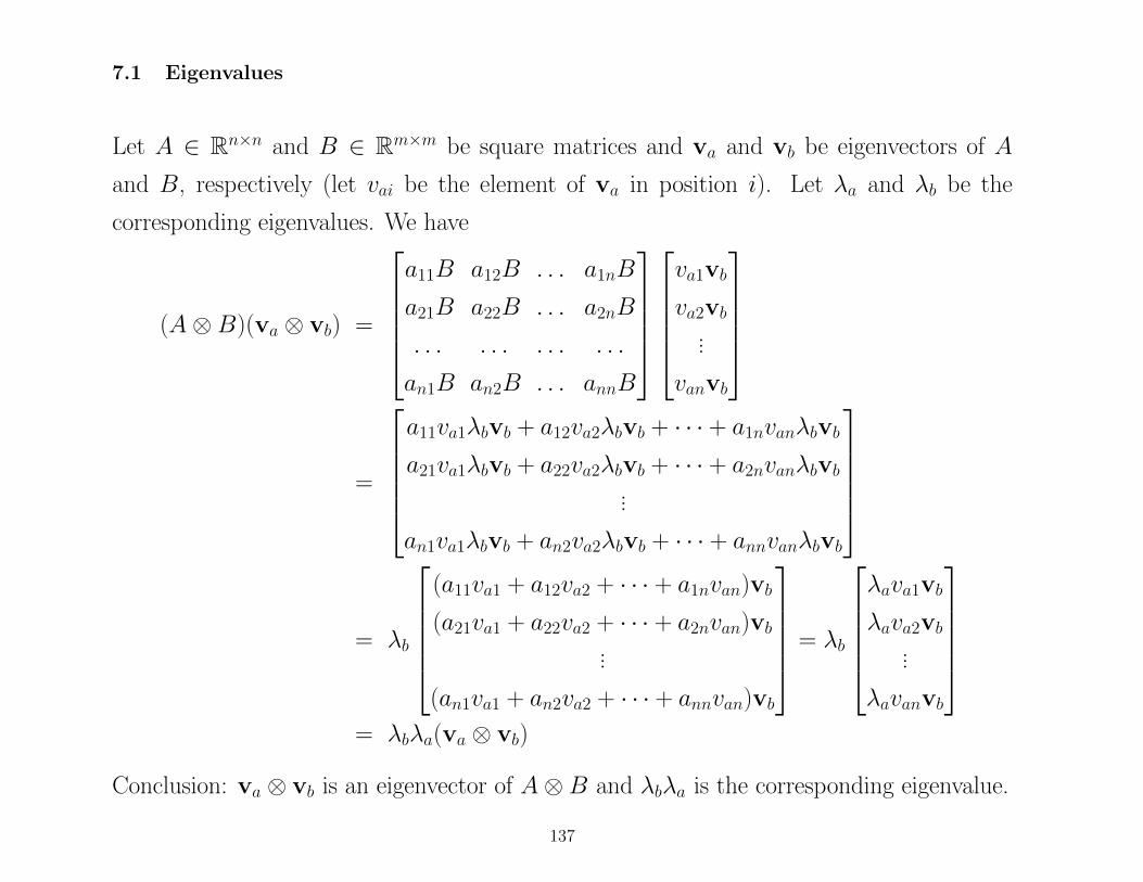
7.1 Eigenvalues
Let A ∈ Rn×n and B ∈ Rm×m be square matrices and va and vb be eigenvectors of A
and B, respectively (let vai be the element of va in position i). Let λa and λb be the
corresponding eigenvalues. We have
(A⊗B)(va ⊗ vb) =
a11B a12B . . . a1nB
a21B a22B . . . a2nB
. . . . . . . . . . . .
an1B an2B . . . annB
va1vb
va2vb...
vanvb
=
a11va1λbvb + a12va2λbvb + · · · + a1nvanλbvb
a21va1λbvb + a22va2λbvb + · · · + a2nvanλbvb...
an1va1λbvb + an2va2λbvb + · · · + annvanλbvb
= λb
(a11va1 + a12va2 + · · · + a1nvan)vb
(a21va1 + a22va2 + · · · + a2nvan)vb...
(an1va1 + an2va2 + · · · + annvan)vb
= λb
λava1vb
λava2vb...
λavanvb
= λbλa(va ⊗ vb)
Conclusion: va ⊗ vb is an eigenvector of A⊗B and λbλa is the corresponding eigenvalue.
137
7.2 Vectorization
Notation. Given a matrix A ∈ Rn×m. We will denote by A[i] be the i-th column of A.
We define vec(A) to be the “vectorization” of A, i.e. the column vector
vec(A) =
A[1]
A[2]
...
A[m]
Lemma 7.1 Let A ∈ Rn×m, P ∈ Rm×p and B ∈ Rp×q. Then
1.
vec(AP ) = (Ip ⊗ A)vec(P )
2.
vec(PB) = (B> ⊗ Im)vec(P )
3.
vec(APB) = (B> ⊗ A)vec(P )
138
Proof.
1.
vec(AP ) =
A(P[1])
A(P[2])...
A(P[p])
=
A 0 . . . 0
0 A . . . 0
0 . . . . . . 0
0 0 . . . A
P[1]
P[2]
...
P[p]
= (Ip ⊗ A)vec(P )
2.
(PB)[j] = (P )B[j] =∑p
i=1 P[i]bij = [b1jI | b2jI | . . . bpjI ]vec(P )
⇒
vec(PB) =
(PB)[1]
(PB)[2]
...
(PB)[q]
=
[b11I | b21I | . . . bp1I ]vec(P )
[b12I | b22I | . . . bp2I ]vec(P )...
[b1qI | b2qI | . . . bpqI ]vec(P )
=
b11I b21I . . . bp1I
b12I b22I . . . bp2I...
b1qI b2qI . . . bpqI
vec(P ) = (B> ⊗ I)vec(P )
139
3.
vec(APB) = (I ⊗ A)vec(PB) = (I ⊗ A)(B> ⊗ I)vec(P )
=
A 0 . . . 0
0 A . . . 0
0 . . . . . . 0
0 0 . . . A
b11I b21I . . . bp1I
b12I b22I . . . bp2I...
b1qI b2qI . . . bpqI
vec(P ) = (B> ⊗ A)vec(P )
Remark 7.1 Notice that in most formulas, if the matrices are complex instead of real the
transpose is replaced by conjugate transpose. For formulas vec(PB) = (B> ⊗ Im)vec(P )
and vec(APB) = (B>⊗A)vec(P ). The transpose remain transpose even in the complex
case.
140
7.3 Mixing ordinary and Kronecker products: The mixed-product prop-
erty
The following theorem is fundamental.
Theorem 7.1 If A, B, C and D are matrices such that the matrix products AC and
BD are well defined, then
(A⊗B)(C ⊗D) = AC ⊗BD (7.68)
Proof. It is sufficient to show that for each vector p of appropriate dimensions, we have
[(A⊗B)(C ⊗D)]p = [AC ⊗BD]p. Given p, let P be such that p = vec(P ). We have:
vec(BDPC>A>) = vec[(BD)P (AC)>] = [(AC)⊗ (BD)]vec(P )
we also have
vec(BDPC>A>) = vec(B(DPC>)A>) = (A⊗B)vec(DPC>) = [(A⊗B)(C⊗D)]vec(P )
Corollary 7.1 If the ordinary products are well defined we have
(A⊗B)(C ⊗D)(E ⊗ F ) = ACE ⊗BDF (7.69)
141
Problem 7.1 Assume that A and B are square matrices of dimension n × n and
m×m. Show that:
1. det(A⊗B) = det(A)n det(B)m INVERTIRE L’ORDINE !!
2. A⊗B is non-singular if and only if A and B are non-singular; moreover, in this
case,
(A⊗B)−1 = A−1 ⊗B−1
3. If A and B are diagonalizable then A⊗B is diagonalizable.
4. Find an expression for the characteristic polynomial of A ⊗ B in terms of the
characteristic polynomials of A and B .
Hint. Write the characteristic polynomials ofA andB in the form pA(s) =∏n
i=1(s−λi),pB(s) =
∏mi=1(s− µi), and use the previous corollary.
Problem 7.2 Let A ∈ Rn×m and B ∈ Rp×q. Show that
(A⊗B)+ = A+ ⊗B+.
142
Problem 7.3 Assume that A and B are square matrices. Show that:
1. ‖A⊗B‖2 = ‖A‖2‖B‖2, where ‖ · ‖2 is the spectral norm, i.e. ‖A‖2 = max Σ(A).
2. For any k = 1, 2, . . . , (I ⊗ A)k = I ⊗ Ak and (A⊗ I)k = Ak ⊗ I.
3. exp(I ⊗ A) = I ⊗ exp(A) and exp(A⊗ I) = exp(A)⊗ I.
4. I ⊗ A and B ⊗ I commute.
143
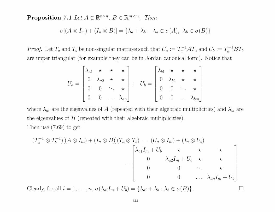
Proposition 7.1 Let A ∈ Rn×n, B ∈ Rm×m. Then
σ[(A⊗ Im) + (In ⊗B)] = λa + λb : λa ∈ σ(A), λb ∈ σ(B)
Proof. Let Ta and Tb be non-singular matrices such that Ua := T−1a ATa and Ub := T−1
b BTb
are upper triangular (for example they can be in Jordan canonical form). Notice that
Ua =
λa1 ? ? ?
0 λa2 ? ?
0 0 . . . ?
0 0 . . . λan
; Ub =
λb1 ? ? ?
0 λb2 ? ?
0 0 . . . ?
0 0 . . . λbm
where λai are the eigenvalues of A (repeated with their algebraic multiplicities) and λbi are
the eigenvalues of B (repeated with their algebraic multiplicities).
Then use (7.69) to get
(T−1a ⊗ T−1
b )[(A⊗ Im) + (In ⊗B)](Ta ⊗ Tb) = (Ua ⊗ Im) + (In ⊗ Ub)
=
λa1Im + Ub ? ? ?
0 λa2Im + Ub ? ?
0 0 . . . ?
0 0 . . . λanIm + Ub
Clearly, for all i = 1, . . . , n, σ(λaiIm + Ub) = λai + λb : λb ∈ σ(B).
144
7.4 Lyapunov equations
Let A ∈ Rn×n, Q ∈ Rn×n. The equations
AP + PA> = Q, P − APA> = Q
pop up in stability theory of linear differential/difference systems
x(t) = Ax(t) , x(k + 1) = Ax(k)
Continuous-time Lyapunov Equations
AP + PA> = Q
This equation admits a solution P ⇐⇒ vec(AP + PA>) = vec(Q) admits a solution P .
Now,
vec(AP + PA>) = [I ⊗ A + A⊗ I ]vec(P )
Hence equation AP + PA> = Q admits a solution P iff the equation
[I ⊗ A + A⊗ I ] p = vec(Q)
admits a solution p or equivalently iff
vec(Q) ∈ Im [I ⊗ A + A⊗ I ]
145
Question: When does equation
AP + PA> = Q
admit solutions for all matrices Q?
Answer: If and only if Im [I ⊗ A + A ⊗ I ] = Rn2 equivalent to [I ⊗ A + A ⊗ I ] being
invertible i.e. no zero eigenvalues
λ1 + λ2 6= 0, ∀λ1, λ2 ∈ σ(A)
A does not have pairs of opposite eigenvalues.
In this case the solution is unique. In fact its vectorization vec(P ) is given by
vec(P ) = [I ⊗ A + A⊗ I ]−1vec(Q).
Definition 7.2 If A does not have pairs of opposite eigenvalues we say that the spec-
trum of A is continuous-time unmixed. In this case we will also say that A is continuous-
time unmixed.
Problem 7.4 If for given A and Q, equation AP + PA> = Q has a unique solution
P then is it true that A is continuous-time unmixed?
146
7.5 Symmetry
With vectorization we completely loose control over symmetry! When Q is symmetric, we
want to impose that the solution P is symmetric.
Lemma 7.2 Assume that the spectrum of A is continuous-time unmixed and that
Q = Q>. Then the unique solution of AP + PA> = Q is symmetric.
Proof. Let P be a solution of AP + PA> = Q = Q> = P>A> + AP>. Then A(P −P>) + (P − P>)A> = 0. Let ∆ := P − P>. We have A∆ + ∆A> = 0. Since A has
continuous-time unmixed spectrum this equation has a unique solution which is ∆ = 0.
Hence, P = P>.
Problem 7.5 Prove that if Q = Q> and equation AP + PA> = Q admits solutions
then it also admits symmetric solutions.
Hint. Compute Q+Q>
2 .
147
In conclusion:
Theorem 7.2 Given A ∈ Rn×n, the following facts are equivalent:
1. The spectrum of A is continuous-time unmixed.
2. Equation AP + PA> = Q admits solutions for any matrix Q ∈ Rn×n.
3. Equation AP + PA> = Q admits a unique solution P for any matrix Q ∈ Rn×n.
4. If Q is such that equation AP + PA> = Q admits solutions then the solution is
unique (i.e. AP1 + P1A> = AP2 + P2A
> implies P1 = P2).
5. For any Q = Q> there is a unique solution P of equation AP +PA> = Q which is
symmetric.
148
Discrete-time Lyapunov Equations
P − APA> = Q
This equation admits a solution P iff equation
vec(P − APA>) = vec(Q)
admits a solution P . Now,
vec(P − APA>) = [I − A⊗ A]vec(P )
In conclusion, equation P − APA> = Q admits a solution P iff equation
[I − A⊗ A] p = vec(Q)
admits a solution p or equivalently iff
vec(Q) ∈ Im [I − A⊗ A]
149
Question: When does equation
P − APA> = Q
admit solutions for all matrices Q?
Answer: If and only if Im [I−A⊗A] = Rn2 ⇐⇒ [I−A⊗A] is invertible ⇐⇒ λ1λ2 6= 1,
∀λ1, λ2 ∈ σ(A)⇐⇒ A does not have pairs of reciprocal eigenvalues.
In this case the solution is unique. In fact its vectorization vec(P ) is given by
vec(P ) = [I − A⊗ A]−1vec(Q).
Definition 7.3 If A does not have pairs of reciprocal eigenvalues we say that the
spectrum of A is discrete-time unmixed. In this case we will also say that A is discrete-
time unmixed.
Problem 7.6 Prove that, if given A and Q, equation P − APA> = Q has a unique
solution P then A is discrete-time unmixed.
150
What about symmetry?
With vectorization we completely loose control over symmetry! When Q is symmetric, we
want to impose that the solution P is symmetric.
Problem 7.7 Assume that Q = Q>. Prove that:
1. If the spectrum of A is discrete-time unmixed, then the unique solution P of
equation P − APA> = Q, is symmetric.
2. If equation P − APA> = Q admits solutions then it also admits symmetric solu-
tions.
151
In conclusion:
Theorem 7.3 Given A ∈ Rn×n, the following facts are equivalent:
1. The spectrum of A is discrete-time unmixed.
2. Equation P − APA> = Q admits solutions for any matrix Q ∈ Rn×n.
3. Equation P − APA> = Q admits a unique solution P for any matrix Q ∈ Rn×n.
4. If Q is such that equation P − APA> = Q admits solutions then the solution is
unique (i.e. P1 − AP1A> = P2 − AP2A
> implies P1 = P2).
If the above conditions hold then for any Q = Q> the unique solution P of equation
P − APA> = Q is symmetric.
7.6 Sylvester equations
Let A ∈ Rn×n, B ∈ Rm×m and Q ∈ Rm×n. We now consider the equation
AP − PB = Q
in the unknown P ∈ Rm×n.
This is called Sylvester equation and is more general than the continuous-time Lyapunov
equation which can be recovered by setting m = n and B = −A>.
152
Problem 7.8 Given A ∈ Rn×n and B ∈ Rm×m, the following facts are equivalent:
1. A and B have non-intersecting spectra: σ(A) ∩ σ(B) = ∅.
2. Equation AP − PB = Q admits solutions for any matrix Q ∈ Rn×n.
3. Equation AP − PB = Q admits a unique solution P for any matrix Q ∈ Rn×n.
4. If Q is such that equation AP − PB = Q admits solutions then the solution is
unique (i.e. AP1 − P1B = AP2 − P2B implies P1 = P2).
Hint. The proof is similar to that for the Lyapunov equation (recall that σ(B) = σ(B>)).
153
7.7 General Stein equations
Let A ∈ Rn×n, B ∈ Rm×m and Q ∈ Rm×n. We now consider the equation
APB − P = Q
in the unknown P ∈ Rm×n.
This is called Stein equation and is more general than the discrete-time Lyapunov equation
which can be recovered by setting m = n and B = A>.
Problem 7.9 Given A ∈ Rn×n and B ∈ Rm×m, the following facts are equivalent:
1. ∀λa ∈ σ(A), λb ∈ σ(B), λaλb 6= 1.
2. Equation APB − P = Q admits solutions for any matrix Q ∈ Rn×n.
3. Equation APB − P = Q admits a unique solution P for any matrix Q ∈ Rn×n.
4. If Q is such that equation APB − P = Q admits solutions then the solution is
unique.
Hint. The proof is similar to that for the discrete-time Lyapunov equation.
154
Inertia Theorems
For an Hermitian matrix H with π positive, ν negative and δ zero eigenvalues, we shall call
the ordered triple
In (H) = (π, ν, δ )
the inertia of H . More generally, for an n × n matrix A which has π eigenvalues with
positive real part, ν with negative real part, and δ purely imaginary ones, we shall again
call the the triple (π, ν, δ ) the inertia of A, and write In (A) = (π, ν, δ ). Next we state a
number of inertia theorems mostly due to H. Wimmer [12, 13].
Two square matrices A and B are said to be congruent if there is an invertible matrix S
such that SAS∗ = B. Congruence is clearly an equivalence relation. By far the most well-
known result about congruence is Sylvester Law of Inertia which describes an important
invariant with respect to congruence.
Theorem 7.4 (Sylvester) Let A, B be Hermitian matrices. Then A and B are
congruent if and only if they have the same inertia.
155
Theorem 7.5 (Wimmer) Let H be Hermitian. If
AH + HA∗ = BB∗
and (A, B) is a controllable pair, then In (H) = In (A). In particular, δ(H) = δ(A).
Definition 7.4 Suppose A ∈ Cn×n. Let n<(A), n>(A), n1(A) be the number of eigen-
values λ of A with |λ| < 1, |λ| > 1, and |λ| = 1, respectively. We call
In d(A) := (n<(A), n>(A), n1(A) )
the discrete inertia of A.
For the discrete Lyapunov equation we have
Theorem 7.6 Let (A, B) be a reachable pair and let H be a Hermitian solution of
the discrete Lyapunov equation
H = AHA∗ + BB∗.
Then H > 0 if and only if |λ(A)| < 1; that is
In (H) = (n, 0, 0) ⇔ In d(A) = (n, 0, 0)
156
and H < 0 if and only if |λ(A)| > 1; i.e.
In (H) = ( 0, n, 0) ⇔ In d(A) = ( 0, n, 0)
Moreover H is non-singular if and only if A has no eigenvalues of absolute value 1;
i.e.
δ(H) = 0 ⇔ n1(A) = 0
In fact,
In (H) = In d(A) .
Note that the inverse H−1 of an invertible Hermitian H has the same inertia of H . In fact,
H = HH−1H = H∗H−1H .
157
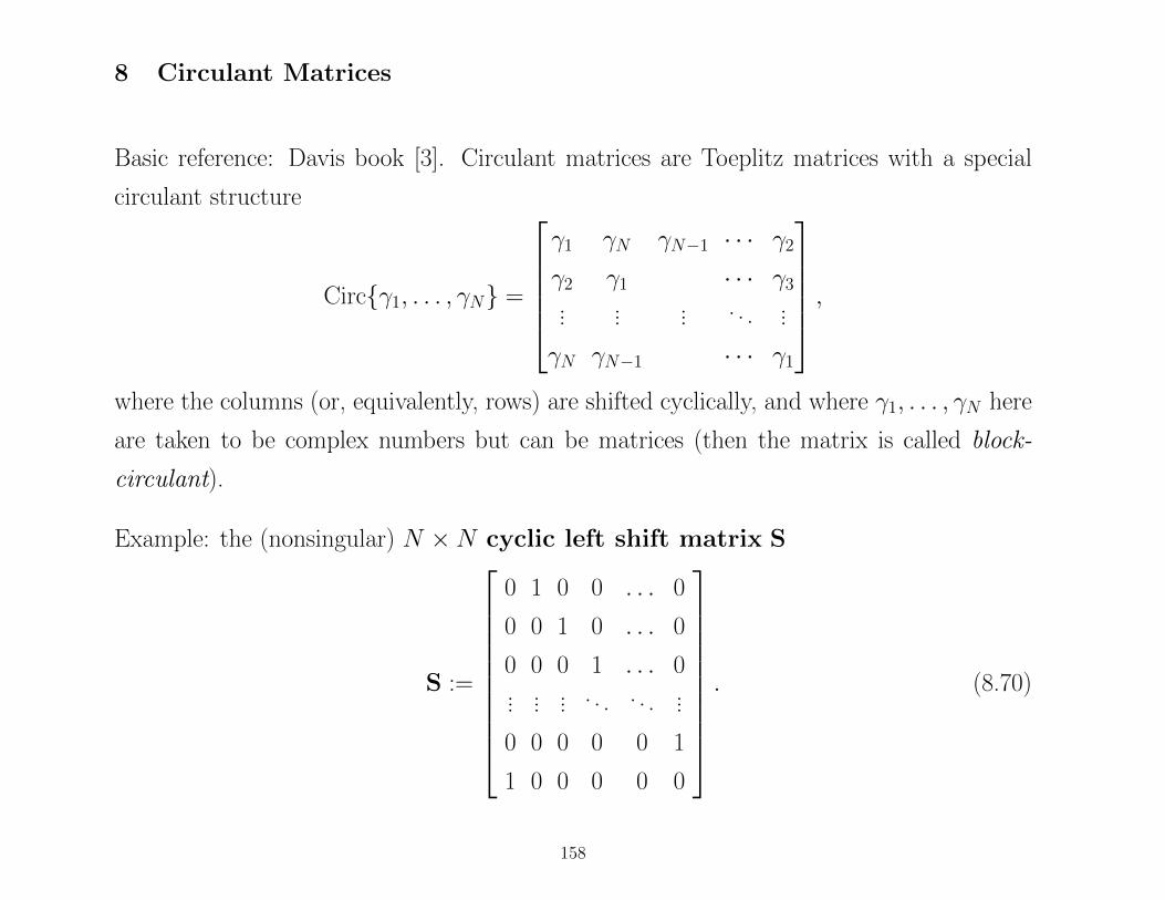
8 Circulant Matrices
Basic reference: Davis book [3]. Circulant matrices are Toeplitz matrices with a special
circulant structure
Circγ1, . . . , γN =
γ1 γN γN−1 · · · γ2
γ2 γ1 · · · γ3
... ... ... . . . ...
γN γN−1 · · · γ1
,where the columns (or, equivalently, rows) are shifted cyclically, and where γ1, . . . , γN here
are taken to be complex numbers but can be matrices (then the matrix is called block-
circulant).
Example: the (nonsingular) N ×N cyclic left shift matrix S
S :=
0 1 0 0 . . . 0
0 0 1 0 . . . 0
0 0 0 1 . . . 0... ... ... . . . . . . ...
0 0 0 0 0 1
1 0 0 0 0 0
. (8.70)
158
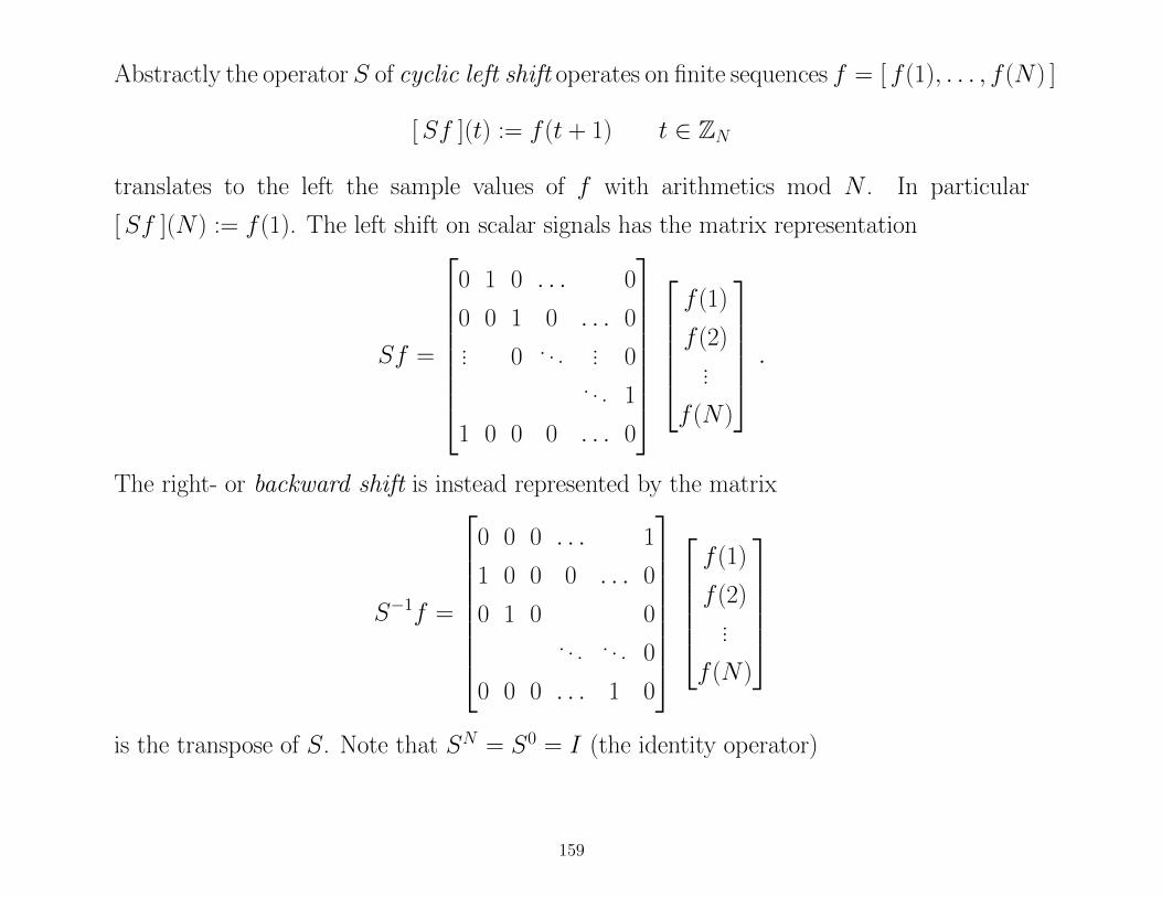
Abstractly the operator S of cyclic left shift operates on finite sequences f = [ f (1), . . . , f (N) ]
[Sf ](t) := f (t + 1) t ∈ ZN
translates to the left the sample values of f with arithmetics mod N . In particular
[Sf ](N) := f (1). The left shift on scalar signals has the matrix representation
Sf =
0 1 0 . . . 0
0 0 1 0 . . . 0... 0 . . . ... 0
. . . 1
1 0 0 0 . . . 0
f (1)
f (2)...
f (N)
.
The right- or backward shift is instead represented by the matrix
S−1f =
0 0 0 . . . 1
1 0 0 0 . . . 0
0 1 0 0. . . . . . 0
0 0 0 . . . 1 0
f (1)
f (2)...
f (N)
is the transpose of S. Note that SN = S0 = I (the identity operator)
159
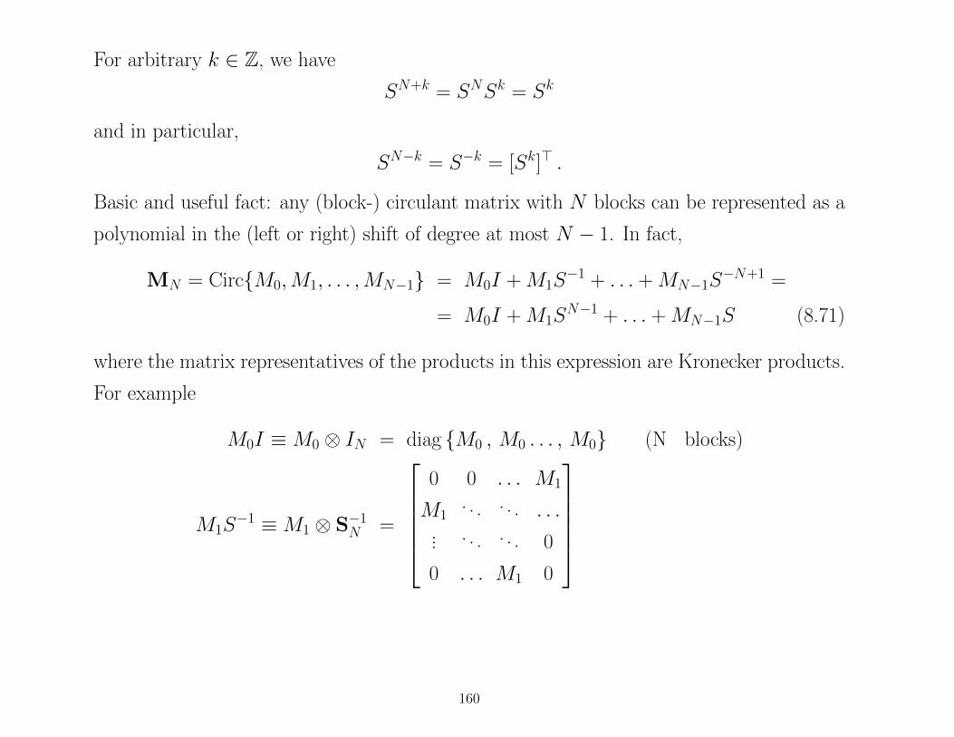
For arbitrary k ∈ Z, we have
SN+k = SNSk = Sk
and in particular,
SN−k = S−k = [Sk]> .
Basic and useful fact: any (block-) circulant matrix with N blocks can be represented as a
polynomial in the (left or right) shift of degree at most N − 1. In fact,
MN = CircM0,M1, . . . ,MN−1 = M0I + M1S−1 + . . . + MN−1S
−N+1 =
= M0I + M1SN−1 + . . . + MN−1S (8.71)
where the matrix representatives of the products in this expression are Kronecker products.
For example
M0I ≡M0 ⊗ IN = diag M0 , M0 . . . , M0 (N blocks)
M1S−1 ≡M1 ⊗ S−1
N =
0 0 . . . M1
M1. . . . . . . . .
... . . . . . . 0
0 . . . M1 0
160
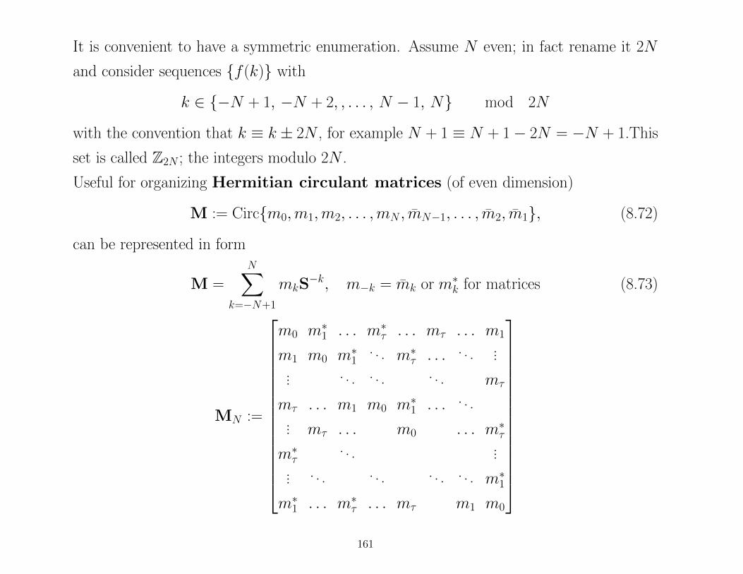
It is convenient to have a symmetric enumeration. Assume N even; in fact rename it 2N
and consider sequences f (k) with
k ∈ −N + 1, −N + 2, , . . . , N − 1, N mod 2N
with the convention that k ≡ k ± 2N , for example N + 1 ≡ N + 1− 2N = −N + 1.This
set is called Z2N ; the integers modulo 2N .
Useful for organizing Hermitian circulant matrices (of even dimension)
M := Circm0,m1,m2, . . . ,mN , mN−1, . . . , m2, m1, (8.72)
can be represented in form
M =
N∑k=−N+1
mkS−k, m−k = mk or m∗k for matrices (8.73)
MN :=
m0 m∗1 . . . m∗τ . . . mτ . . . m1
m1 m0 m∗1. . . m∗τ . . . . . . ...
... . . . . . . . . . mτ
mτ . . . m1 m0 m∗1 . . . . . .... mτ . . . m0 . . . m∗τ
m∗τ. . . ...
... . . . . . . . . . . . . m∗1
m∗1 . . . m∗τ . . . mτ m1 m0
161
8.1 The Symbol of a Circulant
If
MN = CircM0,M1, . . . ,MN−1
The polynomial M(ζ) =∑N−1
k=0 Mkζ−k is called the symbol of M, it plays important role
in the analysis.
For now the variable ζ can be taken to be complex but this will be refined after introducing
the Fourier transform.
Problem 8.1 In how many equivalent ways can you represent the polynomial M(ζ) ?
For Hermitian circulants the symbol can be written
M(ζ) =
N∑k=−N+1
Mkζ−k, M−k = M ∗
k
(we want it to look like a Z-transform).
162
8.2 The finite Fourier Transform
The finite Fourier transform is a mapping from functions defined on Z2N onto complex-
valued functions on the unit circle of the complex plane, regularly sampled at intervals of
length ∆ := π/2N . We shall call this object the discrete unit circle and denote it by T2N .
This Fourier map is usually called the discrete Fourier transform (DFT).
Let ζ1 := ei∆ be the primitive 2N -th root of unity; i.e., ∆ = π/N , and define the discrete
variable ζ taking the 2N values
ζk ≡ ζk1 = ei∆k ; k = −N + 1, . . . , 0, . . . , N
running counterclockwise on the discrete unit circle T2N . In particular, we have ζ−k = ζk
(complex conjugate).
The discrete Fourier transform F maps a finite signal g = gk; k = −N + 1, . . . , N, into
a sequence of complex numbers
g(ζj) :=
N∑k=−N+1
gkζ−kj , j = −N + 1,−N + 2, . . . , N. (8.74)
163
It is well-known that the signal g can be recovered from its DFT g by the formula
gk =
N∑j=−N+1
ζkj g(ζj)∆
2π, k = −N + 1,−N + 2, . . . , N, (8.75)
where ∆2π = 1
2N plays the role of a uniform discrete measure with total mass one on the
discrete unit circle T2N . It may look nicer to write (8.75) as an integral
gk =
∫ π
−πeikθg(eiθ)dν(θ), k = −N + 1,−N + 2, . . . , N,
where ν is a step function with steps 12N at each ζk; i.e.,
dν(θ) =
N∑j=−N+1
δ(eiθ − ζj)dθ
2N.
In particular, we have ∫ π
−πeikθdν(θ) = δk0,
where δk0 equals one for k = 0 and zero otherwise.
164
The Fourier transform is a map between finite-dimensional inner product spaces. It is a
unitary map i.e. preserves the inner products: If f is the DFT of fk,N∑
k=−N+1
fkgk =1
2N
N∑k=−N+1
f (ζk)g(ζ−k)
=
∫ π
−πf (eiθ)g(eiθ)∗dν(θ).
(8.76)
This is Plancherel’s Theorem (Parseval formula) for the DFT.
To prove these facts it is convenient to write the discrete Fourier transform (8.74) in matrix
form
g = Fg, (8.77)
where g :=(g(ζ−N+1), g(ζ−N+2), . . . , g(ζN)
)>, g := (g−N+1, g−N+2, . . . , gN)> and F is the
nonsingular 2N × 2N Vandermonde matrix
F =
ζN−1−N+1 ζN−2
−N+1 · · · ζ−N−N+1
... ... · · · ...
ζN−10 ζN−2
0 · · · ζ−N0... ... · · · ...
ζN−1N ζN−2
N · · · ζ−NN
. (8.78)
which is circulant and unitary (in the Euclidean metrics !)
165
Since F is a unitary matrix can compute the inverse
g =1
2NF∗g,
i.e., F−1 corresponds to 12NF∗. Consequently, FF∗ = 2N I, and hence F−1 = 1
2NF∗ and
(F∗)−1 = 12NF.
The Parseval-Plancherel formula also follows from the fact that F is unitary.
Problem 8.2 What are the eigenvalues of the Vandermonde matrix (8.78) ?
8.3 Back to Circulant matrices
Recall that a circulant matrix can be represented as a polynomial in the shift
M =
N∑k=−N+1
mkS−k,
where S is the nonsingular 2N × 2N cyclic shift matrix which is itself a circulant matrix
with symbol S(ζ) = ζ .
Recall that S2N = S0 = I, and
Sk+2N = Sk, S2N−k = S−k = (Sk)>.
166
We shall now interpret ζ as a discrete complex variable running on the discrete unit cir-
cle T2N .
Apply the DFT to the shift of a sequence. If g := (g−N+1, g−N+2, . . . , gN)>,
[Sg]k = gk+1, k ∈ Z2N . (8.79)
so that
F(Sg)(ζ) = ζF(g)(ζ)
and by linearity of the DFT we have
F(Mg)(ζ) = m(ζ)F(g)(ζ), (8.80)
where m(ζ) is the symbol of the circulant matrix M.
m(ζ) =
N∑k=−N+1
mkζ−k
We may interpret the symbol m(ζ) as the Fourier transform of the circulant.
167
Theorem 8.1 All circulant matrices of the same size are diagonalized by the discrete
Fourier transform. More precisely, are simultaneously diagonalizable by the unitary
matrix 1√2N
F
M =1
2NF∗diag
(m(ζ−N+1),m(ζ−N+2), . . . ,m(ζN)
)F, (8.81)
In particular
S =1
2NF∗diag
(ζ−N+1, . . . , ζN
)F
S∗ =1
2NF∗diag
(ζ−1−N+1, . . . , ζ
−1N
)F,
Problem 8.3 Prove Theorem 8.1 using the above diagonalization of the shift.
Problem 8.4 Prove that the condition
SMS∗ = M, (8.82)
is both necessary and sufficient for M to be circulant.
168
Use the diagonalization of Theorem 8.1 to see that, formally, the inverse M−1 is
M−1 =1
2NF∗diag
(m(ζ−N+1)−1, . . . ,m(ζN)−1
)F,
Is this a circulant? Use the diagonalization of S and S∗ to verify that
SM−1S∗ = M−1.
Consequently, M−1 is also a circulant matrix with symbol m(ζ)−1. Therefore there must be
a pseudo polynomial in ζ which is equivalent to m(ζ)−1. The coefficients of the equivalent
pseudo-polynomial m(ζ) can be determined by Lagrange interpolation.
In general, in view of the circulant property, quotients of symbols are themselves pseudo-
polynomials of degree at most N and hence symbols.
Theorem 8.2 If A and B are circulant matrices of the same dimension with symbols
a(ζ) and b(ζ) respectively, then AB and A + B are circulant matrices with symbols
a(ζ)b(ζ) and a(ζ) + b(ζ), respectively.
In mathematical jargon, the circulant matrices of a fixed dimension form an algebra – more
precisely, a commutative *-algebra with the involution * being the conjugate transpose
– and the DFT is an algebra homomorphism of the set of circulant matrices onto the
pseudo-polynomials of degree at most N in the variable ζ ∈ T2N .
169
References
[1] Ben-Israel A., GrevilleT. N. E., Generalized Inverses: Theory and Applications,
Wiley, New York, 1974.
[2] Bertero M. and Boccacci P. Introduction to inverse problems in imaging, CRC Press,
1998.
[3] P.J. Davis, Circulant Matrices, second ed., AMS Chelsea Publishing 1994.
[4] P.A. Fuhrmann, A polynomial Approach to Linear Algebra, second ed., Springer
2010.
[5] Gantmacher F. R. Theory of Matrices, Voll. I e II, Chelsea, New York 1959.
[6] G.H. Golub “Numerical methods for solving linear least-squares problems”, Nu-
merische Mathematik, 7, pp.206-216, 1965.
[7] G.H. Golub and C. Van Loan, Matrix Computations, the Johns Hopkins Un. Press
1983; pdf scaricabile dalla rete.
[8] P.R. Halmos , Introduction to Hilbert Space, Chelsea 1957.
[9] C.L. Lawson and R.J. Hanson, Solving Least Squares Problems, Prentice Hall, En-
glewood Cliffs, 1974.
170
[10] G. Picci, Filtraggio Satatistico (Wiener, Levinson, Kalman) e applicazioni, ed.
Libreria Progetto, Padova, 2007.
[11] G. Strang, Linear Algebra and its Applications 4th ed., Thomson 2006 (original first
ed. Academic Press, 1976).
[12] H. Wimmer, On the Ostrowski-Schneider Inertia Theorem J. Math. Analysis and
Applications, 41 pp 164–169, 1973.
[13] H. Wimmer and A Ziebur, Remarks on inertia theorems for matrices Czechoslovak
Mathematical Journal, 25 pp 556–561, 1975.
171