applications manual for portable … · proton magnetometer, is a scalar measurement, ... 4...
TRANSCRIPT
APPLICATIONS MANUAL
FOR
PORTABLE MAGNETOMETERS
byS. BREINER
Geometrics2190 Fortune Drive
San Jose, California 95131 U.S.A.
Copyright 1999 by Geometrics. All Rights Reserved . Printed in theUnited States of America. This publication, or parts thereof, may not be reproduced in any form without permission of Geometrics.
i
PREFACE
This Manual was written to satisfy most of the needs ofthe average user of a portable total field magnetometerfor both conventional and unconventional applications,including geological exploration, search for lost objects,magnetic measurements of rock or iron specimens andarchaeological prospecting. As the name implies, this isa manual or guide for professional and non-professionalpersons who may not have the time, the requisite back-ground or the ready access to the proper libraries todelve deeply into standard texts, the few that there are,on applied geophysics.
Some of the information that I have included in thisManual may be found in the references cited or drawnfrom obscure sources, or uncovered amongst equationsand confusing terminology in physics or engineeringtexts. Many of the facts and instructions in this Manual,however, do not appear anywhere else in print. Forexample, I know of no other readily available referenceon the subjects of magnetic search of buried objects,many of the portable gradiometer applications, opera-tional considerations of proton magnetometers and theeffect of electrical currents on portable total field mag-netometers. Among the less common subjects that arecovered are the magnetic properties and detection ofcommon steel objects, facts concerning the detectionof buried ruins, methods for sketch-it-yourself anomalyconstruction, and some help in interpreting anomaliesat the magnetic equator. I also tried to simplify someaspects of the potentially complex subject of magneticsusing short-cuts wherever possible and deskilling some-what the fine art of magnetic interpretation. For mostportable magnetometer work, I feel this approach isquite adequate. Certainly for the more sophisticatedtechniques required for interpretation of the usually-more-precise aeromagnetic surveys, the reader isadvisedto consult the References or persons knowledgeable inthe subject.
Figures and examples are used liberally in the explana-tions because I feel they assist or confirm one’s under-standing of these subjects. Almost all of the profileswere drawn free-hand according to the techniquesdescribed and should not be considered as precisecomputer-derived curves. They do demonstrate that onecan be his own ‘magnetics expert’ insofar as what isrequired for most of these applications.
The question of units always arises in any technicalpublication. Many magnetic measurements, particularlymagnetic properties of rocks and geophysical research,use cgs, some physics and engineering applications usemks, while geophysical exploration, for most of thereaders of this Manual, still utilizes feet and miles. A mix-ture of units, hopefully not too confusing, was thereforeunavoidable. Subsequent editions of this Manual may bewritten specifically in carefully selected metric units.
The various chapters were prepared to be read or utilizedindependent of each other if necessary. For example,someone interested in using the magnetometer forarchaeology but who does not particularly enjoy wadingthrough the mathematics of Chapter V, can proceeddirectly to Chapter VII. He would be aided, however, bysubsequently skimming through Chapter V.
I would appreciate criticism or suggestions should any-one note errors or have suggestions on how I may im-prove later editions. Moreover, if the reader finds thatmy explanations or facts fall just short of what isrequired, I am available by telephone or through writtencorrespondence.
SHELDON BREINERGeoMetrics
395 Java DriveSunnyvale, California 94066Telephone: (408) 734-4616
iii
Contents
I
II
III
IV
INTRODUCTION. . . . . . . . . . . . . . . . . . . . . . . . . . . . . . . . . . . . . . . . . . . . . . . 1
MAGNETOMETERS
Instrument Use . . . . . . . . . . . . . . . . . . . . . . . . . . . . . . . . 3Proton Magnetometer .........................3Total Field Measurement ......................3Limitations of a Proton Magnetometer .......... 4
EARTH’S FIELD MAGNETISM
Introduction . . . . . . . . . . . . . . . . . . . . . . . . . . . . . . . . . . .Time Variations ...............................6Magnetic Minerals and Iron .................... 6Induced Magnetization ........................8Remanent or Permanent Magnetization ......... 8
FIELD PROCEDURESAND DATA REDUCTION
Magnetic Cleanliness and Sensor Positions. ... 11Operational Considerations ................... 11
Valid Reading Vs. Noise .................. 11Sensor Orientation .......................12instrument Readings ..................... 12Correction for Time Variations ............ 12High Magnetic Gradients ................. 13
Data Reduction ..............................13Profile Smoothing ........................13Removal of Regional Gradients ........... 14Contour Maps ............................14Construction of a Contour Map ........... 15
V INTERPRETATION
P r e f a c e . . . . . . . . . . . . . . . . . . . . . . . . . . . . . . . . . . . . . . . i i i
Introduction .................................17Asymmetry ..................................17Depth Dependence. ..........................18Other Anomaly Shape Factors ................ 18Geological Models ...........................18Elementary Dipoles and Monopoles ........... 18
Simplified Method for Total Field Signature. ... 19Earth’s Field Component Behavior ........ 20Dipoles Vs. Monopoles
Vs. Arrays of Poles ..................... 20Configuration of Field Lines .............. 20Dipole and Monopole Fall-Off Factor ...... 20Dipole Factor-of-Two ..................... 20Application of Method .................... 20
Contour Presentation ofDipole and Prism Anomalies ................ 22
Anomaly Amplitude .......................... 24Amplitude Estimates
for Common Sources . . . . . . . . . . . . . . . . . . .24Dipole and Monopole Signatures
in Vertical and Horizontal Fields ........ 24Maximum Amplitude Given
Magnetization and Generalized Form .... 26Anomaly Depth Characteristics ............... 28
Anomaly Width ................ , .......... 28Anomaly Depth Estimation ................ 28Identification of Anomaly . . . . . . . . . . . . . . . . . 29Fall-Off Rate . . . . . . . . . . . . . . . . . . . . . . . . . . . . . 29Assumptions on Maximum
Amplitude and Depth Estimates . . . . . . . . . 29Half Width Rules .......................... 31Slope Techniques ......................... 31Other Depth Estimating Methods .......... 31
Interpretation Summary . . . . . . . . . . . . . . . . . . . . . . 3 2
VI MAGNETIC SUSCEPTIBILITY,MAGNETIZATION AND MAGNETICMOMENT MEASUREMENTS
Introduction . . . . . . . . . . . . . . . . . . . . . . . . . . . . . . . . . . .33Applications .................................33Procedures . . . . . . . . . . . . . . . . . . . . . . . . . . . . . . . . . . . 3 4Random Sample Rotation
for Magnitude Only ......................... 34Systematic Rotation
for Magnitude and Direction ................ 35Dipole in Earth’s Field ........................ 36Non-Spherical Object Rotation .............. .36
(continued)
V
Contents (continued)
VII MAGNETIC SEARCH
Introduction . . . . . . . . . . . . . . . . . . . . . . . . . . . . . . . . . 39Determination of Object Magnetism . . . . . . . . . . . 39Detectability . . . . . . . . . . . . . . . . . . . . . . . . . . . . . . . . . 39Magnetic Anomaly Signatures . . . . . . . . . . . . . . . . 39Depth/Amplitude Behavior . . . . . . . . . . . . . . . . . . . . 39Search Procedures. . . . . . . . . . . . . . . . . . . . . . . . . . .4 1
Determination of Magnetic MomentVs. Search Grid Vs. Resolution ........... 41
T r a v e r s e s . . . . . . . . . . . . . . . . . . . . . . . . . . . . . . . . 4 1Detailed Mapping
for Pinpointing Location .............. 41Special Search Topics . . . . . . . . . . . . . . . . . .42
Iron and Steel ............................42Permanent Vs.
Induced Anomaly Sources . . . . . . . . . .. 42Pipelines (horizontal) ............................... 44Magnetic Markers ........................ 44
Archaeological Exploration ................... 45Introduction .............................45Magnetic Anomalies
of Archaeological Origin ................ 45Remanent Magnetization ................. 46Archaeomagnetism ....................... 46Magnetization and
Susceptibility of Soils .................. 46Remanent Magnetization of Soils .......... 47Magnetic Anomaly Complexity ............. 47
VIII GRADIOMETERS AND GRADIENT TECHNIQUES
Introduction . . . . . . . . . . . . . . . . . . . . . . . . . . . . . . . . .49Applications of the Gradiometer . . . . . . . . . . . . . . 49Conditions for Gradient Measurement . . . . . . . . . 49Gradiometer Sensitivity ........................ 50Gradiometer Readings in the Field . . . . . . . . . . . . 50Gradiometer as a Filter . . ......................... 50Calculation of Vertical Gradient ................. 51Depth Estimates from Vertical Gradients ........ 52General Expression Involving
Gradients and Coordinates ................. 53Gradient Vector Diagrams and
Vector Information from Total Field .......... 54
I X MAGNETIC MEASUREMENTS OFELECTRIC CURRENT DISTRIBUTIONS
Archeological Survey Planningand Feasibility .................... .47
Archaeological Anomaly Amplitudeand Signatures ................... .47
Introduction . . . . . . . . . . . . . . . . . . . . . . . . .. 55Applications ................................. .55Configuration of Magnetic Field of
Electric Current Sources .................... 55Amplitude of Fields of Current Sources .......... 56
REFERENCES ......................... 58
I.
INTRODUCTION
This Manual is intended for use as a general guide for a number of very diverse applications of portablemagnetometers, especially the total field proton (nuclear precession) magnetometers. The diversityof applications and the general complexity of magnetic field measurements limits the depth to whichany one subject can be covered, but further information, if desired, can be obtained through the authoror from any of the references cited.
Among the applications for which this Manual is written are mineral and petroleum exploration, geo-logical mapping, search for buried or sunken objects, magnetic field mapping, geophysical research,magnetic observatory use, measurement of magnetic properties of rocks or ferromagnetic objects,paleomagnetism, archaeological prospecting, conductivity mapping, gradiometer surveying, andmagnetic modeling. The terminology, units of measurement, and assumed prerequisite knowledgeare those employed in the field of geology and geophysics.
II.
MAGNETOMETERS
Instrument Use
The common types of portable magnetometers in usetoday are fluxgate, proton precession, Schmidt fieldbalance, dip needle and other special purpose instru-ments. Field balances and dip needles are mechanicaldevices comprised of pivoted magnets measuring verticalor horizontal intensity or field direction, and are notmuch used today being replaced by the more sensitiveand less cumbersome fluxgate and proton magneto-meters. Portable fluxgate magnetometers employ a satur-able core sensor held in a vertical direction to measurevertical intensity with an effective sensitivity on the orderof several gammas. Fluxgate magnetometers, too, areslowly being replaced by the proton magnetometerwhich has greater sensitivity (1 gamma or better), abso-lute accuracy, no moving parts, and measures total fieldintensity with freedom from orientation errors. For rea-sons of its increasing utilization and because manyapplications require these features, the proton magne-tometer will be the principal instrument under discussionin the Manual. Much of the Manual from Chapters IIIthrough IX nevertheless applies to vertical componentflux gate magnetometers as well. Anomaly signatures athigh latitudes (magnetic dip 70 ° o r greater) are practicallyidentical for the two instruments; at other latitudes theydiffer significantly.
Proton Magnetometer
The proton precession magnetometer is so namedbecause it utilizes the precession of spinning protons ornuclei of the hydrogen atom in a sample of hydrocarbonfluid to measure the total magnetic intensity. The spin-ning protons in a sample of water, kerosene, alcohol,etc., behave as small, spinning magnetic dipoles. Thesemagnets are temporarily aligned or polarized by appli-cation of a uniform magnetic field generated by a currentin a coil of wire. When the current is removed, the spinof the protons causes them to precess about the direc-tion of the ambient or earth’s magnetic field, much as aspinning top precesses about the gravity field. The pre-cessing protons then generate a small signal in the samecoil used to polarize them, a signal whose frequency is
precisely proportional to the total magnetic field intensityand independent of the orientation of the coil, i.e., sensorof the magnetometer. The proportionality constant whichrelates frequency to field intensity is a well known atomicconstant: the gyromagnetic ratio of the proton. The pre-cession frequency, typically 2000 Hz, is measured bymodern digital counters as the absolute value of thetotal magnetic field intensity with an accuracy of 1 gam-ma, and in special cases 0.1 gamma, in the earth’s fieldof approximately 50,000 gammas.
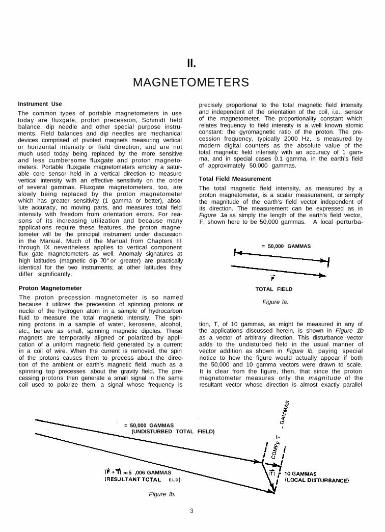
Total Field Measurement
The total magnetic field intensity, as measured by aproton magnetometer, is a scalar measurement, or simplythe magnitude of the earth’s field vector independent ofits direction. The measurement can be expressed as inFigure 1a as simply the length of the earth’s field vector,F, shown here to be 50,000 gammas. A local perturba-
. 5 = 50,000 GAMMAS
TOTAL FIELD
Figure la.
tion, T, of 10 gammas, as might be measured in any ofthe applications discussed herein, is shown in Figure 1bas a vector of arbitrary direction. This disturbance vectoradds to the undisturbed field in the usual manner ofvector addition as shown in Figure lb, paying specialnotice to how the figure would actually appear if boththe 50,000 and 10 gamma vectors were drawn to scale.It is clear from the figure, then, that since the protonmagnetometer measures only the magnitude of theresultant vector whose direction is almost exactly parallel
F = 50,000 GAMMAS (0(UNDISTURBED TOTAL FIELD) @
I -
- 5»» ,006 GAMMASRR E S U L T A N T(RE E L D)
Figure lb.
3
4 APPLICATIONS MANUAL FOR PORTABLE MAGNETOMETERS
to the undisturbed total field vector, that which is mea-sured is very nearly the component of the disturbancevector in the direction of the original undisturbed totalfield, or where
If + fl= F + compFT
where IFI GI.
Such conditions are almost always valid except in thenear field of large steel objects or in the vicinity of ironore deposits or certain ultrabasic rocks which produceanomalies larger than 10,000 gammas. Thus, the changein total field, A F = compFT, i.e., the component of theanomalous field, T, in the direction of F. (Except wherenoted, CompFT will be referred to simply as the anomaly
T.) The proton precession magnetometer, for small per-turbations, can therefore be considered to be an earth's-field-determined component magnetometer.
This property of measuring this scalar magnitude of thefield, otherwise called total field intensity, is very signifi-cant with respect to the asymmetric signatures of anom-alies, interpretation of anomalies, and in various specialapplications. Furthermore, the fact that what is measuredis independent of the orientation of the sensor, allowsthe magnetometer to be operated without attention toorientation or leveling such as would be the case with
a fluxgate magnetometer on the mobile platform of aperson, vehicle, or aircraft. The only limitation of sucha scalar measurement, albeit a minor one, is the factthat the component of the anomalous field which ismeasured is not normally under the control of the ob-server, but rather at the whim of the local direction ofthe earth’s magnetic field.
Limitations of a Proton MagnetometerThe proton magnetometer has no moving parts, producesan absolute and relatively high resolution measurementof the field and usually displays the measurement in theform of an unambiguous digital lighted readout. Severaloperational restrictions exist, however, which may be ofconcern under special field conditions. First, the protonprecession signal is sharply degraded in the presence ofa large magnetic field gradient greater than 200 gammasper foot (approximately 600 gammas per meter). Also,the signal amplitude from the sensor is on the order ofmicrovolts and must be measured to an accuracy of0.04 Hz of the precession frequency of several thousandHz. This small signal can be rendered immeasurableby the effects of nearby alternating current electricalpowei sources. For these two reasons, a proton mag-netometer cannot usually be operated within the con-fines of a typical building. Developments and proceduresare presented which minimize these effects for the appli-cations to be described in the Manual.
III.
EARTH’S FIELD MAGNETISM
Introduction
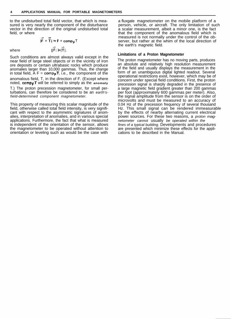
The earth’s magnetic field resembles the field of a largebar magnet near its center or that due to a uniformlymagnetized sphere. The origin of the field is not wellunderstood, but thought to be due to currents in a fluidconductive core. On the surface of the earth the pole ofthis equivalent bar magnet, nearest the north geographi-cal pole, is actually a ‘south’ magnetic pole. Thisparadoxical situation exists since by convention a north-seeking end of a compass needle is defined as pointingnorth yet must point to a pole of opposite sense or southpole of the earth’s magnetic field. To avoid possible con-fusion, though, the magnetic pole near the geographicalnorth pole is, and will be referred to as, a ‘north’ pole.
The field, or flux, lines of the earth exhibit the usualpattern common to a small magnet as shown in Figure 2.Note that the direction of the field is vertical at the northand south magnetic poles, and horizontal at the magneticequator. An understanding of this geometry is importantwith respect to interpretation of magnetic anomalies. Theintensity of the field, which is a function of the densityof the ‘flux lines’ shown in Figure 2, again behaves as abar magnet being twice as large in the polar region as inthe equatorial region, or approximately 60,000 gammasand 30,000 gammas respectively. The inclination from Figure 2.
30 60. 90. 120.
60.
120° 150° 180° 150° 120° 90° 60° 30° 0° 30' 60° 90° 120°
Figure 3. The Geomagnetic Inclination in Degrees of Arc from the Horizontal SOURCE: U.S.N.H.O
5
6 APPLICATIONS MANUAL FOR PORTABLE MAGNETOMETERS
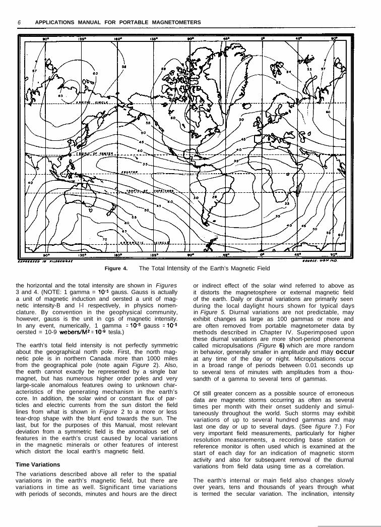
Figure 4. The Total Intensity of the Earth’s Magnetic Field
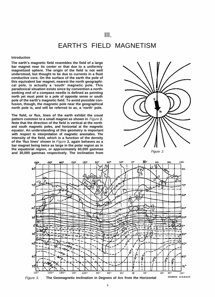
the horizontal and the total intensity are shown in Figures3 and 4. (NOTE: 1 gamma = 10-9 gauss. Gauss is actuallya unit of magnetic induction and oersted a unit of mag-netic intensity-B and l-l respectively, in physics nomen-clature. By convention in the geophysical community,however, gauss is the unit in cgs of magnetic intensity.In any event, numerically, 1 gamma = lo+ gauss = lo+oersted = 10-9 webers/M = 10-9 tesla.)
The earth’s total field intensity is not perfectly symmetricabout the geographical north pole. First, the north mag-netic pole is in northern Canada more than 1000 milesfrom the geographical pole (note again Figure 2). Also,the earth cannot exactly be represented by a single barmagnet, but has numerous higher order poles and verylarge-scale anomalous features owing to unknown char-acteristics of the generating mechanism in the earth’score. In addition, the solar wind or constant flux of par-ticles and electric currents from the sun distort the fieldlines from what is shown in Figure 2 to a more or lesstear-drop shape with the blunt end towards the sun. Thelast, but for the purposes of this Manual, most relevantdeviation from a symmetric field is the anomalous set offeatures in the earth’s crust caused by local variationsin the magnetic minerals or other features of interestwhich distort the local earth’s magnetic field.
Time Variations
The variations described above all refer to the spatialvariations in the earth’s magnetic field, but there arevariations in time as well. Significant time variationswith periods of seconds, minutes and hours are the direct
or indirect effect of the solar wind referred to above asit distorts the magnetosphere or external magnetic fieldof the earth. Daily or diurnal variations are primarily seenduring the local daylight hours shown for typical daysin Figure 5. Diurnal variations are not predictable, mayexhibit changes as large as 100 gammas or more andare often removed from portable magnetometer data bymethods described in Chapter IV. Superimposed uponthese diurnal variations are more short-period phenomenacalled micropulsations (Figure 6) which are more randomin behavior, generally smaller in amplitude and may occurat any time of the day or night. Micropulsations occurin a broad range of periods between 0.01 seconds upto several tens of minutes with amplitudes from a thou-sandth of a gamma to several tens of gammas.
Of still greater concern as a possible source of erroneousdata are magnetic storms occurring as often as severaltimes per month with their onset suddenly and simul-taneously throughout the world. Such storms may exhibitvariations of up to several hundred gammas and maylast one day or up to several days. (See figure 7.) Forvery important field measurements, particularly for higherresolution measurements, a recording base station orreference monitor is often used which is examined at thestart of each day for an indication of magnetic stormactivity and also for subsequent removal of the diurnalvariations from field data using time as a correlation.
The earth’s internal or main field also changes slowlyover years, tens and thousands of years through whatis termed the secular variation. The inclination, intensity

EARTH’S FIELD MAGNETISM 7
MID-NORTHERN AND MID-SOUTHERN LATITUDES
HOURS: 0DAYS:
1200 2400 1200 2400 1200 2400DAY 1 DAY 2 DAY 3
EQUATORIAL LATITUDEAFigure 5. Typical Diurnal Variations in Total Field Intensity
10 MINUTES
Figure 6. Typical Micropulsations
50 GAMMAS
Figure 7. Typical Magnetic Storm
8 APPLICATIONS MANUAL FOR PORTABLE MAGNETOMETERS
and even the location of the poles varies slowly at a raterelevant, in the context of this Manual, only to observa-tory and archival interests. From time-to-time throughgeologic history, the main field has even reversed andthe consequences of these events are extremely impor-tant for a number of portable magnetometer applicationscovered in the Manual.
Magnetic Minerals and IronThe application of portable magnetometers as treatedherein has, as its primary objective, the identificationand description of spatial changes in the earth’s field.The time changes described above simply representnoise or interference in the measurements of interest.The spatial variations or anomalies to be mapped forthese applications are those which might occur overseveral feet or several thousands of feet and are usuallycaused by an anomalous distribution of magnetic miner-als or by iron objects or cultural features which may beof interest. The anomalies from naturally occurring rocksand minerals are due chiefly to the presence of the mostcommon magnetic mineral, magnetite (Fe Fe*O,), or itsrelated minerals, ulvospinel, titanomagnetite, maghemite,etc. which will collectively be referred to as magnetite,a dark, heavy, hard and’ resistant mineral. The rust-colored very common forms of iron oxide are not usuallymagnetic and are seldom related to the source of magne-tic anomalies. Other magnetic minerals which occur to afar lesser extent are ilmenite, pyrrhotite (with sulphidemineralization), and others of even lesser consequence.
All rocks contain some magnetite from very small frac-tions of a percent up to several percent, and even severaltens of percent in the case of magnetic iron ore deposits.The distribution of magnetite or certain characteristicsof its magnetic properties may be utilized in explorationor mapped for other purposes. Iron objects in the earth’smagnetic field, whether something buried or intentionallyplanted for subsequent retrieval, would also create adetectable magnetic anomaly. Cultural features associ-ated with man’s habitation can frequently be detectedthrough magnetic surveys owing to the contrast in mag-netite associated with numerous artificial features suchas man-made structures, voids, or the enhanced mag-netic effects of baked clays and pottery (see Chapter VII).
Induced MagnetizationMagnetic anomalies in the earth’s magnetic field arecaused by two different kinds of magnetism: inducedand remanent (permanent) magnetization. Induced mag-netization refers to the action of the field on the materialwherein the ambient field is enhanced and the materialitself acts as a magnet. The magnetization of such ma-terial is directly proportional to the intensity of the am-bient field and to the ability of the material to enhancethe local field-a property called magnetic susceptibility.The induced magnetization is equal to the product ofthe volume magnetic susceptibility, k, and the earth’s orambient field intensity, F, or
Ii = kF
where Ii is the induced magnetization per unit volumein cgs electromagnetic units, and F is the field intensityin gauss. (Note: in some texts, the specific magneticsusceptibility or susceptibility per unit weight (gram) isused) For most materials, k is much less than 1 and, infact, is usually ilO- cgs or smaller. If k is this small andpositive, the material is said to be paramagnetic and,
when negative, diamagnetic. For magnetite, k is approxi-mate/y 0.3 cgs and is ferrimagnetic while for iron alloys,k may vary between 1 and 1 , 0 0 0 , 0 0 0 and such materialsare called ferromagnetic. Both ferrimagnetic and ferro-magnetic susceptibility are also a function of the fieldintensity in which they are measured. In all cases, in thisManual, the field intensity is assumed to be the ambientearth’s field intensity between 0.3 and 0.6 gauss
A parameter similar to k is the magnetic permeability,cc, which is the ratio of the magnetic induction, B, tothe field intensity, F (Magnetic induction is the magne-tization induced in the material). B includes not only themagnetization of the material, but also the effect of thefield itself and is expressed by
B = F+4171
where B is in gauss. Therefore as stated above,
andp=$
/J = 1 +4nk
Thus when k is very small, as in air, /.J x I and when kis 0.1 or larger I-( is generally one order of magnitudelarger. The susceptibility k can be thought of as theabsolute ability and p the relative ability of a materialto create local magnetization. The measurement of per-meability is most often used for materials where ~1 ismuch greater than 1, typically iron, steel and otherferromagnetic alloys.
Inasmuch as magnetite and its distribution is of suchgreat importance for a number of these applications, itis important to understand its relation to common rocktypes. The susceptibility k of magnetite was given asapproximately 0.3 cgs which may actually vary between0.1 and 1.0 depending upon its grain size and otherproperties. The magnetic susceptibility of a rock con-taining magnetite is simply related to the amount ofmagnetite it contains. For example, rock containing 7%magnetite will have a volume susceptibility of 3 x 10⁻³ cgs,etc. Typical susceptibilities of rocks are given below, butmay vary by an order of magnitude or more in most cases:
altered ultrabasic rocksbasaltgabbrograniteandesiterhyoliteshaleshist and othermetamorphic rocksmost sedimentary rockslimestone and chert
-10-4 to 10-z cgs- 1 0 -4 to 10-3- 1 0 - 4-10-5 to 10-3- 1 o-4-10-5 to 10-4-10-3 to 10-4
-10-4 to 10-S-10-6 to 10-S-1 O-6
Typically, dark, more basic igneous rocks possess ahigher susceptibility than the acid igneous rocks andthe latter, in turn, higher than sedimentary rocks.
Remanent or Permanent MagnetizationThe remanent or permanent magnetization, I,, (the formerascribed to rocks, the latter to metals) is often the predom-inant magnetization (relative to the induced magnetiza-tion) in many igneous rocks and iron alloys. Permanentmagnetization depends upon the metallurgical propertiesand the thermal, mechanical and magnetic history of
EARTH’S FIELD MAGNETISM 9
the specimen, and is independent of the field in whichit is measured. Magnetite may have a remanent magne-tization, lr, of perhaps 0.1 to 1.0 gauss, ordinary ironmay have a permanent magnetization between 1 and 10,and a permanent magnet may be between 100 and 1,000gauss or larger. Chapter VI will describe simple methodsfor measuring both the remanent ,and induced magneti-zations and the magnetic susceptibility of rocks andmiscellaneous objects. Chapter VII more fully describesthe magnetization of iron objects.
The remanent magnetization is of great importance inmapping and interpretation, and in the fields of paleo-magnetism, archaeological exploration, and archaeomag-netism. The remanent magnetization of magnetite is asstated independent of the present earth’s field. By andlarge, the high values of remanent magnetization arerelated to the effects of heating, whether naturally heated,as in the case of igneous rocks, or artificially heated, asin the case of baked clay, pottery, and other man-madeobjects found in archaeological sites. Prior to suchheating, small regions, called domains, within each mag-netite crystal would be more or less randomly-oriented.During heating, particularly at high temperatures, the
domains reorient themselves, which upon cooling, tendto align themselves more or less in the direction of theambient magnetic field and thus parallel to each other,thus creating a net magnetization fixed with respect tothe object. This remanent magnetization may be as muchas 10 or more times greater than the induced magnetiza-tion for many rock types. Thus, the net magnetizationmight be considerably higher than would be indicatedmerely by consideration of the susceptibilities listedabove.
The remanent magnetization of a rock or object may ormay not be in the same directionn as the present earth’sfield for the object may have been reoriented and becausethe earth’s field is known to have changed its orientationin geologic and even historic time. Rocks are frequentlyreversely magnetized so that measurement of this rem-anent magnetization is a useful aid to interpretation ifthe rocks which produce an observed anomaly are,indeed, accessible. The fields of paleomagnetism andarchaeomagnetism in particular depend upon the precisedetermination of the orientation of the ‘frozen paleo-field’ as it is measured in a given rock or other specimen,and methods for measuring such will be described inChapter VI.
IV.
FIELD PROCEDURES AND DATA REDUCTION
Magnetic Cleanliness and Sensor PositionsMost of the applications for portable magnetometersrequire that the operator be relatively free of magneticmaterials on his person. The importance of checkingoneself cannot be over-estimated if measurements onthe order of 1 gamma are desired. In field surveys, theusual magnetic material one may have may include, ofcourse, the obvious such as a rock pick, Brunton comp-pass, pocket knife, or instrument console and the not-so-obvious effects of the pivot in eyeglasses, the pants clip atthe top of men’s trousers, the light meter in a camera,the magnet in the speaker of a tape recorder, metal in aclipboard, some mechanical pencils, some keychains,and the steel shank in one’s shoes or boots. Of course,some of these items cannot be altered or left behindand some are not significant in any event. The sensoritself should be kept clean to avoid possible contamina-tion by magnetite-bearing dirt on the sensor surface.In order to check the ‘heading effect’, i.e., the effect oforientation on the observed field intensity during a fieldsurvey, the operator can take readings at each of thefour cardinal directions while pivoting about the positionof the sensor and note the changes. If the maximumchange is typically less than 10 gammas, the averagereadings on a line will probably not be affected by morethan 5 gammas and individual readings by less than thisinasmuch as readings along the profile are more-or-lessalong a given heading f perhaps 30” about one orienta-tion. If a sensitivity of 1 gamma is desired, the headingerror should be less than several, preferably 2 gammasor less and depending upon the desired sensitivity, theoperator should make some effort to face in the samedirection, if possible, for all readings on a given traverse.
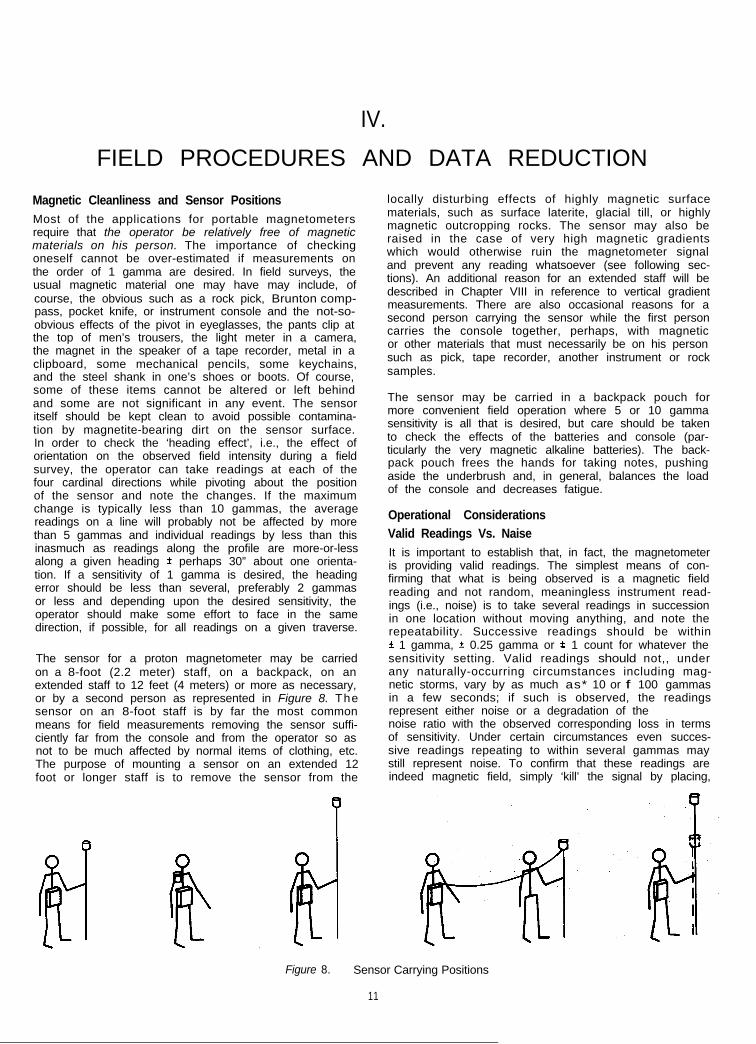
The sensor for a proton magnetometer may be carriedon a 8-foot (2.2 meter) staff, on a backpack, on anextended staff to 12 feet (4 meters) or more as necessary,or by a second person as represented in Figure 8. Thesensor on an 8-foot staff is by far the most commonmeans for field measurements removing the sensor suffi-ciently far from the console and from the operator so asnot to be much affected by normal items of clothing, etc.The purpose of mounting a sensor on an extended 12foot or longer staff is to remove the sensor from the
ti i
locally disturbing effects of highly magnetic surfacematerials, such as surface laterite, glacial till, or highlymagnetic outcropping rocks. The sensor may also beraised in the case of very high magnetic gradientswhich would otherwise ruin the magnetometer signaland prevent any reading whatsoever (see following sec-tions). An additional reason for an extended staff will bedescribed in Chapter VIII in reference to vertical gradientmeasurements. There are also occasional reasons for asecond person carrying the sensor while the first personcarries the console together, perhaps, with magneticor other materials that must necessarily be on his personsuch as pick, tape recorder, another instrument or rocksamples.
The sensor may be carried in a backpack pouch formore convenient field operation where 5 or 10 gammasensitivity is all that is desired, but care should be takento check the effects of the batteries and console (par-ticularly the very magnetic alkaline batteries). The back-pack pouch frees the hands for taking notes, pushingaside the underbrush and, in general, balances the loadof the console and decreases fatigue.
Operational ConsiderationsValid Readings Vs. NaiseIt is important to establish that, in fact, the magnetometeris providing valid readings. The simplest means of con-firming that what is being observed is a magnetic fieldreading and not random, meaningless instrument read-ings (i.e., noise) is to take several readings in successionin one location without moving anything, and note therepeatability. Successive readings should be withinf 1 gamma, + 0.25 gamma or f 1 count for whatever thesensitivity setting. Valid readings should not,, underany naturally-occurring circumstances including mag-netic storms, vary by as much as* 10 or f 100 gammasin a few seconds; if such is observed, the readingsrepresent either noise or a degradation of the signal-to-noise ratio with the observed corresponding loss in termsof sensitivity. Under certain circumstances even succes-sive readings repeating to within several gammas maystill represent noise. To confirm that these readings areindeed magnetic field, simply ‘kill’ the signal by placing,
Figure 8. Sensor Carrying Positions
11
12 APPLICATIONS MANUAL FOR PORTABLE MAGNETOMETERS
momentarily during the reading, something magneticadjacent to the sensor such as one’s shoe, watch, certainrocks, etc. Random readings varying by 10 or 100 gam-mas or more would then be observed in addition to theirdeviating considerably from the readings without theobject present. Another but less certain method is totake readings at intervals of increasing distance from anobject or location known to produce a magnetic anomaly.
Typical reasons for a proton magnetometer not producingvalid readings may be: electrical noise from AC powerlines, transformers or other radiating sources; high mag-netic gradients from underlying rocks, nearby visible orhidden iron objects, fence lines or improvised iron hard-ware improperly used nea the sensor; improper orienta-tion of the sensor (even when ‘omni-directional’) ; expiredbatteries, incorrect range setting or instrumen t failuresbroken or nearly broken sensor cable, and other mal-functions usually described in the instrument operatingmanual.
Valid but distorted readings may result from severalother conditions including the above effects of highmagnetic gradients, magnetic dirt or other magneticcontamination on the sensor and any magnetic bias onthe operator. Time variations (Chapter III and following)and the effects of direct current in distant power linesand trains (Chapter IX) can also distort magneticobseryations.
Sensor OrientationAccording to the theory of operation of the proton mag-netometer, the total intensity, measured as the frequencyof precession, is independent of the orientation of thesensor. Th e amplitude of the signal, however, doesvary (as sir+ @ with the angle between the directionof the applied field within the sensor and the earth’sfield direction. Variation of signal amplitude does notnormally affect the readings unless there is simply insuf-ficient signal to be measured accurately, i.e., a minimumsignal amplitude is required above which a variation inamplitude does not affect the readings.
Ideally, the applied field in the sensor should be atright angles to the earth’s field direction. The directionof the applied field is governed by the configuration ofthe polarizing coils in the sensor which are commonlyeither solenoids (cylindrical) or toroids (ring or dough-nut-shaped). The solenoid produces an applied fieldparallel to its axis, whereas the toroid produces a fieldwhich is ring-shaped about the axis of the toroid (con-sult the instrument operations manual to determine thedirection of these axes with respect to the sensor hous-ing). Solenoids are used because they produce some-what higher signal than a toroid and are less perturbedby electrical noise, whereas a toroid is inherently omni-directional. In the ideal case, a solenoid should be heldhorizontal and in any direction in a vertical field, andshould be held vertical in a horizontal (equatorial) fieldfor maximum signal amplitude. A toroidal sensor shouldbe held with its axis vertical in a vertical field, and point-ing north in an equatorial field to obtain maximum sig-nal. A field which dips greater or less than 45’, shouldbe treated as though it were a vertical or horizontalfield respectively.
Instrument ReadingsMeasurements are normally made at regular intervalsalong a grid or otherwise selected path whose locations
are noted for subsequent plotting. Simple pacing isusually adequate with readings every 6, 10, 50, 100,500,or even 1,000 feet (2 to 300 meters), as anomalies, field,and either geological or search requirements dictate.Traverses may be selected along pathways or otheraccessible routes and occasional locations noted on anaerial photograph or map using paced distances inbetween. The density of readings along the traverseshould be related to the wavelength of anomalies ofinterest such that several readings are obtained for anysuch anomaly. A single trial line with relatively densestations is usually attempted first to determine the re-quired station density. It is important never to hold themagnetometer sensor within one or two feet of theground, if possible, in order to avoid effects of minorplacer magnetite which usually collects on the surfaceof the ground, and also to avoid the effects of micro-topography or outcropping rock surfaces.
Readings may be noted in a field notebook or, if desired,on a miniature tape recorder, but care must be takento magnetically compensate the speaker magnet andmotor following the theory given in Chapter VI if one isto use a recorder. The convenience of the recorder isthat only one hand is needed and the data may beplayed back for fast, convenient plotting.
Correction for Time VariationsSome ground magnetic surveys require correction fordiurnal and micropulsation time variations. Correctionis required if the anomalies of interest are broad (thou-sands of feet) and typically less than 20 to 50 gammas,or if the profile lines are very long, or if the objectiveof the survey is a good magnetic contour map expres-sive of deep-seated anomaly sources. Also, if the surveyis performed in the high magnetic latitudes in the auroralzone where typical micropulsations are 10 to 100 gam-mas, correction for such variations would be necessary.On the other hand, if one is merely interested in profileinformation of anomalies of several hundred gammas orif the anomalies are only 20 gammas but can be traversedcompletely in less than 5 minutes, no time variationcorrection is needed. Perhaps most surveys fit the lattercriteria an d do not actually require any such correctionfor time variations.
The simplest method of correcting for time variationsinvolves repeated readings in the same orientation atthe same station at different times during the survey.If a smooth curve is drawn through the readings plottedas a function of time (every hour or so), these valuescan be subtracted from all other readings provided thateach reading also includes the time at which it wasobserved. To avoid an extremely long and repeatedwalk to a single reference station, it is also possible to‘double-back’ to take a second or third reading on eachgiven traverse to determine at least the time variationsfor that traverse. Still another technique is to emulatewhat is done on aeromagnetic surveys, namely, obtainrapidly acquired measurements on tie lines or lineswhich cross the principal traverse lines at each endand perhaps in the center. The stations common to eachtraverse and tie lines should be known and occupiedwhile facing the same direction to avoid heading errors.The simplest method for using these tie lines is to makeeach intersection agree by linearly distributing the erroron each traverse line and holding the tie line valuesfixed-provided the ti e line data were acquired rapidly.
FIELD PROCEDURES AND DATA REDUCTION 13
A local recording base station, i.e., diurnal station moni-tor, is the most ideal method and certainly the mostaccurate for removing time variations. The time varia-tions can readily be removed from each reading, againassuming that the time is noted for each reading on thetraverse to within a minute or so of the base station.The base station should not be further away than 100miles from the area of the survey for agreement withina few gammas and should be positioned more than 200feet away from local traffic and other disturbances (seeChapter VII). The diurnal base station, if left to continuerecording during each evening, can indicate magneticstorms in progress and may be examined at the startof a survey day to determine if any useful measurementscan actually be obtained during such conditions. Duringa magnetic storm, it is best not to obtain field data withthe objective of removing the storm variations as thesurvey magnetometer and base station may not agreebetter than 5 or 10 gammas.
High Magnetic Gradients
In the case where an extremely high magnetic gradientdestroys the signal as evidenced by successive non-repeating measurements, it may be necessary to raisethe sensor up to 10 or 12, sometimes 15 feet in orderto move the sensor to a region of lower gradient. Thiswill only happen over outcropping or nearly outcroppinglarge masses of perhaps altered ultrabasic rocks, mag-netic iron ore deposits or ore bodies containing a largepercent of pyrrhotite and in the near vicinity of buriediron objects in the applications for search. Such anevent would only occur if the gradient exceeds severalhundred gammas per foot. If the span of high gradientis not too wide, it may not actually be necessary toobtain measurements precisely at the highest gradient.Measurements on either side of the anomaly can beextrapolated or be used to at least indicate the contactsof such a highly magnetized formation. Furthermore,as the signal disappears and the readings diverge con-siderably from f 1 or 2 counts, it may be worthwhile tonote approximate indications of magnetic field gradientwhich on some instruments is displayed on the frontpanel as signal amplitude (which is a function of gradient).In areas of highly magnetic surface conditions, as notedin a previous section but where a signal is still obtained,another alternative in acquiring meaningful data otherthan that of using an extended staff would be to make2 to 5 measurements per station, for example, at thepoints of a cross centered at the actual primary stationlocation. The average of these readings would later beused to draw a profile. In this way, some of the surfacenoise is averaged out.
In the absence of anomalous surface conditions and forreasons more fully described in Chapter VIII, it may beuseful for both geological and search applications tomeasure the vertical gradient of the total field. Thevertical gradient is obtained by making 2 total fieldmeasurements, one over another, taking the differencein the readings and dividing by the distance betweenthem.
Data Reduction
The profiles when plotted should be smoothly varyingand expressive of the anomalies of interest. (NOTE:The nature of the disturbances or anomalies of interest,their w i d t h character, signature, and amplitude are dis-cussed in Chapter V, following.) Should there be anexcessive amount of such geologic/magnetic noise, at a
wavelength much shorter or much longer than is ofinterest, it is possible to apply simple filtering or smooth-ing techniques to facilitate interpretation of the profile.As a rule of thumb, never remove or filter out anomalieswhose wavelength is on the order of the depth to sourcesof interest. A number of advanced techniques for dataenhancement or filtering as employed in airborne sur-veys or well-gridded ground surveys will not be dis-cussed within the scope of the Manual but are listedto acknowledge their existence: vertical derivatives,upward and downward continuation, reduction-to-the-pole, bandpass filtering, trend surface filtering, spectralanalysis, trend enhancement, magnetization filtering,and others most of which are applied to two-dimensionaldata.
Profile Smoothing
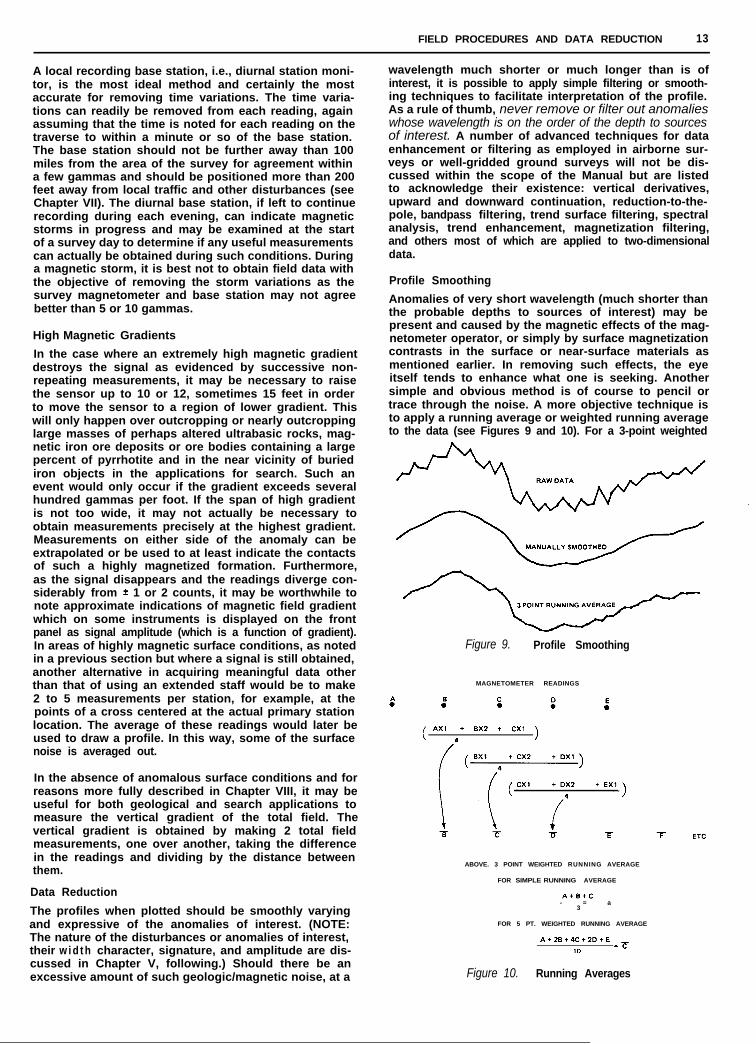
Anomalies of very short wavelength (much shorter thanthe probable depths to sources of interest) may bepresent and caused by the magnetic effects of the mag-netometer operator, or simply by surface magnetizationcontrasts in the surface or near-surface materials asmentioned earlier. In removing such effects, the eyeitself tends to enhance what one is seeking. Anothersimple and obvious method is of course to pencil ortrace through the noise. A more objective technique isto apply a running average or weighted running averageto the data (see Figures 9 and 10). For a 3-point weighted
Figure 9. Profile Smoothing
MAGNETOMETER READINGS
.” :
( AX1d + sx2 + cx’ )
ABOVE. 3 POINT WEIGHTED RUNNING AVERAGE
FOR SIMPLE RUNNING AVERAGE
AtStC- = a
3
FOR 5 PT. WEIGHTED RUNNING AVERAGE
A+ZS+4C+2D+E
10--c
Figure 10. Running Averages

14 APPLICATIONS MANUAL FOR PORTABLE MAGNETOMETERS
running average, for example, one would multiply thevalue at a given station by 2, add the values of the twoadjacent stations, divide the sum by 4. This value is thenset aside for that station for later recompilation of a newprofile while advancing to the next station to performthe same procedure (see figure 10). A 5-point runningaverage might utilize a weighting factor of 4 for the cen-tral point, 2 for each adjacent point, and 1 for the out-side points while dividing by 10 to obtain the averagedvalue. More sophisticated techniques are also possiblesuch as polynomial curve fitting, least squares, digitalbandpass filtering, etc. The number of points or intervalover which the averaging or filtering is to be performedfor removal of such ‘noise’ should be much shorter(perhaps 11~ to I/& than the anomalies of interest.
Removal of Regional GradientsIn most cases, the anomalies of interest usually appearsuperimposed on a much broader anomaly which is notof interest. This broader anomaly, or regional gradient,due to the main earth’s field or very deep or distantsources, may appear simply as a component of slope intne curve and although it is subjectively determined, isoften removed from the data in order to better examinethe anomaly. This gradient is removed from a singleprofile as shown by Figure 11 by drawing a straight lineor broadly-curved line through the non-anomalous por-tions o f the curve. The values are then subtracted ateach station and replotted to present the ‘residual’values, hopefully expressing only the anomalies ofinterest which in this case would be the anomaliesoccurring at the shallower depths. The vertical gradient,measured according to the methods prescribed inChapter VIII, also serves to remove or largely reducethe regional gradient.
Contour MapsMost survey traverses are not sufficiently close nor well-arranged in plan to allow the compilation of a contourmap. Such is usually the case when only mineral explor-
ation data are desired, in broad reconnaissance surveys,or when surveying in extremely rugged terrain wherelarge areas are otherwise inaccessible. Profiles are, infact, usually adequate particularly for anomaly sourceswith very long, horizontal dimensions. Contour maps arenevertheless useful in cases where little is known of thegeology or magnetic sources, where the anomalysources are either small or extremely large, or for ascer-taining, on a more objective basis, the distribution of theanomalous masses or very subtle longer wavelengthfeatures. Many surveys for search also require broadcoverage and perhaps contour map presentation. Analternative to the construction of contour maps forbroad two-dimensional coverage is the presentation of‘offset profiles’ or profiles plotted on abscissae whichalso serve to show the location of the traverse linesdrawn on a map.
Constructing a contour map requires that large effectsfrom diurnal variations or the heading effects, if any, beremoved; that is, that there be a single datum level forall traverses or readings. The process of removing theregional gradients, as described above, frequentlyserves to remove these other sources of errors as welland is satisfactory as long as one is not interested inthe longer wavelength anomalies removed as part ofthe gradient.
The following guide should be useful to one not familiarwith the techniques of constructing a magnetic contourmap, or plan view of the anomalous total intensity. Acontour or iso-intensity map is analogous to a topo-graphic map and is a map on which are drawn lines(contours) of equal intensity, at convenient and regularintensity intervals, as would be observed were a mag-netometer used to occupy every point on the surfaceof the ground. The contoured values are at best extrapo-lations and interpolations across areas where measure-ments are not actually taken. Such a map is drawnwith the knowledge that the magnetic field is smoothly
LINEAR REGIONAL
NON-LINEAR REGIONAL
Figure 11. Removal of Regional GradientRESIDUAL

FIELD PROCEDURES AND DATA REDUCTION 15
varying and on the assumption that one is interestedonly in broad features expressed by such a map. Fea-tures much smaller than the spacing between adjacenttraverses should be examined on a profile basis only andshould not be sought nor included on a map presentation.
Construction of a Contour Map
Given a set of readings obtained on a traverse, the timevariations, if significant, should be removed, perhaps theregional gradient removed and the profiles smoothed.Values are then selected from these smoothed profilesat widely-spaced intervals not less than, say, I/* or l/d thespacing between adjacent traverses or at similarly spacedbut significant points on the profile, namely, maxima,minima, inflection points, etc. In other words, the valuesto be contoured should be more-or-less equally distrib-uted in plan view. Anomalous features which ‘obviously’extend across several traverses might be included also.The total intensity values thus selected and representa-
tive of the principal features are posted at their properlocations on a base map made of material which willsupport numerous erasing of penciled lines and includingreferences to location.
Examine the dynamic range of the values and select 5or 10 intensity levels through this range at convenientvalues such as every 20, 100, or 1000 gammas. Drawthese contours according to the instructions below andthen fill in the intermediate contour lines, i.e., every 10,50, or 500 gamma contours, depending upon whichcoarse valuse above were originally selected, until con-
/
tours appear in all segments of the map. Magneticintensity values and contours should, in theory, besmoothly varying and should thus be smoothed at thelater stages of contouring by removing sharp bends orcorners. After such smoothing, other contour lines asneeded to cover the map adequately are carefully drawnbetween the fair-drawn contours and appropriate labelsapplied. In areas of steep gradients, only a few coarsecontour lines are drawn to avoid numerous and insigni-ficant fine details. Since closed contours (closures)appear the same for maxima and minima, they are dif-ferentiated by applying hashure marks or other indica-tions on the inside of the minima.
The position of the various contours is selected bymanually (eye and mental calculation or by using pro-portional dividers, although not really necessary) inter-polating linearly between all the neighboring values asshown in Figure 72. In this case, it was decided to drawcontours at 10 gamma intervals. The contour line neardata point value 91 would subsequently be smoothedto pass through this data point following the guidelinesgiven above.
Contour lines should never cross nor pass between pairsof data points which are both higher or both lower thanthe value of the contour. Also in some regions of zeroor near zero gradient such as at a saddle point (regionbetween two adjacent maxima or minima), there existsan ambiguity in the direction of the lines. However, itdoes not matter under such conditions which of the twopossible sets of contours are drawn.
0
/,081‘/*SO
9or’ 89
---*!’
/
l 75 //
\ /kc
0 80 l 84 /0
80+ c 0/ - g o -
/ ) I0 l 96
90: 00
l 85-““,/ ’-@ 910 /
0\9c / I/100,
I .’*\
90, 0 100 /‘ I
/’ 1 /*-l 101
l 97 //
l 92
096 D A T A* 90 MANUALLY INTERPOLATED POINT
- - - CONTOURS DRAWN THROUGHINTERPOLATED POINTS
Figure 12. Interpolation and Contouring
v.INTERPRETATION
Introduction
Total magnetic intensity disturbances or anomalies arehighly variable in shape and amplitude; they are almostalways asymmetrical, sometimes appear complex evenfrom simple sources, and usually portray the combinedmagnetic effects of several sources. Furthermore, thereare an infinite number of possible sources which canproduce a given anomaly. The apparent complexity ofsuch anomalies is a consequence of the net effect ofseveral independent but relatively simple functions ofmagnetic dipole behavior. With an understanding ofthese individually simple functions however, and givensome reasonable assumptions regarding the geology,buried object or whatever other source one is seekingto understand, a qualitative but satisfactory interpreta-tion can usually be obtained for most anomaly sources.
The interpretation, explanation and guide presentedhere is directed primarily towards a qualitative interpre-tation for both geological reasons as well as searchapplications, i.e., an understanding of what causes theanomaly, its approximate depth, configuration, perhapsmagnetite content or mass, and other related factors.But even if qualitative information is derived from thedata, it is important to have applied a reasonable amountof care in obtaining precise measurements. Quantitativeinterpretations are possible, but are applied more to air-borne data, entail relatively complex methods for depthdetermination, and are the basis for a relatively largebody of literature on the subject, references to whichare given in the Manual.
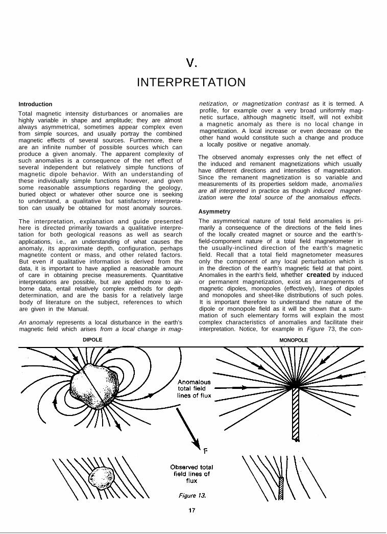
An anomaly represents a local disturbance in the earth’smagnetic field which arises from a local change in mag-
DIPOLE
netization, or magnetization contrast as it is termed. Aprofile, for example over a very broad uniformly mag-netic surface, although magnetic itself, will not exhibita magnetic anomaly as there is no local change inmagnetization. A local increase or even decrease on theother hand would constitute such a change and producea locally positive or negative anomaly.
The observed anomaly expresses only the net effect ofthe induced and remanent magnetizations which usuallyhave different directions and intensities of magnetization.Since the remanent magnetization is so variable andmeasurements of its properties seldom made, anomaliesare all interpreted in practice as though induced magnet-ization were the total source of the anomalous effects.
Asymmetry
The asymmetrical nature of total field anomalies is pri-marily a consequence of the directions of the field linesof the locally created magnet or source and the earth’s-field-component nature of a total field magnetometer inthe usually-inclined direction of the earth’s magneticfield. Recall that a total field magnetometer measuresonly the component of any local perturbation which isin the direction of the earth’s magnetic field at that point.Anomalies in the earth’s field, whether created by inducedor permanent magnetization, exist as arrangements ofmagnetic dipoles, monopoles (effectively), lines of dipolesand monopoles and sheet-like distributions of such poles.It is important therefore to understand the nature of thedipole or monopole field as it will be shown that a sum-mation of such elementary forms will explain the mostcomplex characteristics of anomalies and facilitate theirinterpretation. Notice, for example in Figure 73, the con-
MONOPOLE
18 APPLICATIONS MANUAL FOR PORTABLE MAGNETOMETERS
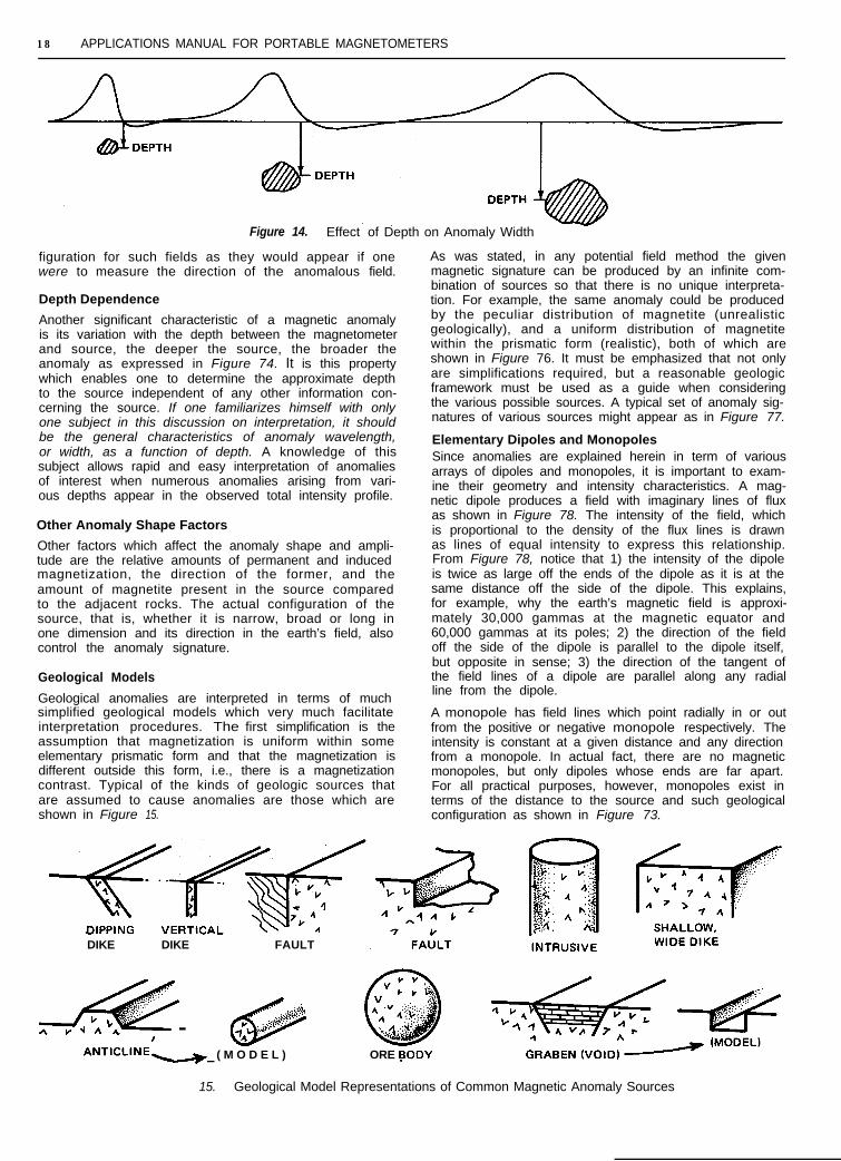
Figure 14. Effect of Depth on Anomaly Width
figuration for such fields as they would appear if onewere to measure the direction of the anomalous field.
Depth Dependence
Another significant characteristic of a magnetic anomalyis its variation with the depth between the magnetometerand source, the deeper the source, the broader theanomaly as expressed in Figure 74. It is this propertywhich enables one to determine the approximate depthto the source independent of any other information con-cerning the source. If one familiarizes himself with onlyone subject in this discussion on interpretation, it shouldbe the general characteristics of anomaly wavelength,or width, as a function of depth. A knowledge of thissubject allows rapid and easy interpretation of anomaliesof interest when numerous anomalies arising from vari-ous depths appear in the observed total intensity profile.
Other Anomaly Shape Factors
Other factors which affect the anomaly shape and ampli-tude are the relative amounts of permanent and inducedmagnetization, the direction of the former, and theamount of magnetite present in the source comparedto the adjacent rocks. The actual configuration of thesource, that is, whether it is narrow, broad or long inone dimension and its direction in the earth’s field, alsocontrol the anomaly signature.
Geological Models
Geological anomalies are interpreted in terms of muchsimplified geological models which very much facilitateinterpretation procedures. The first simplification is theassumption that magnetization is uniform within someelementary prismatic form and that the magnetization isdifferent outside this form, i.e., there is a magnetizationcontrast. Typical of the kinds of geologic sources thatare assumed to cause anomalies are those which areshown in Figure 15.
DIKE DIKE FAULT
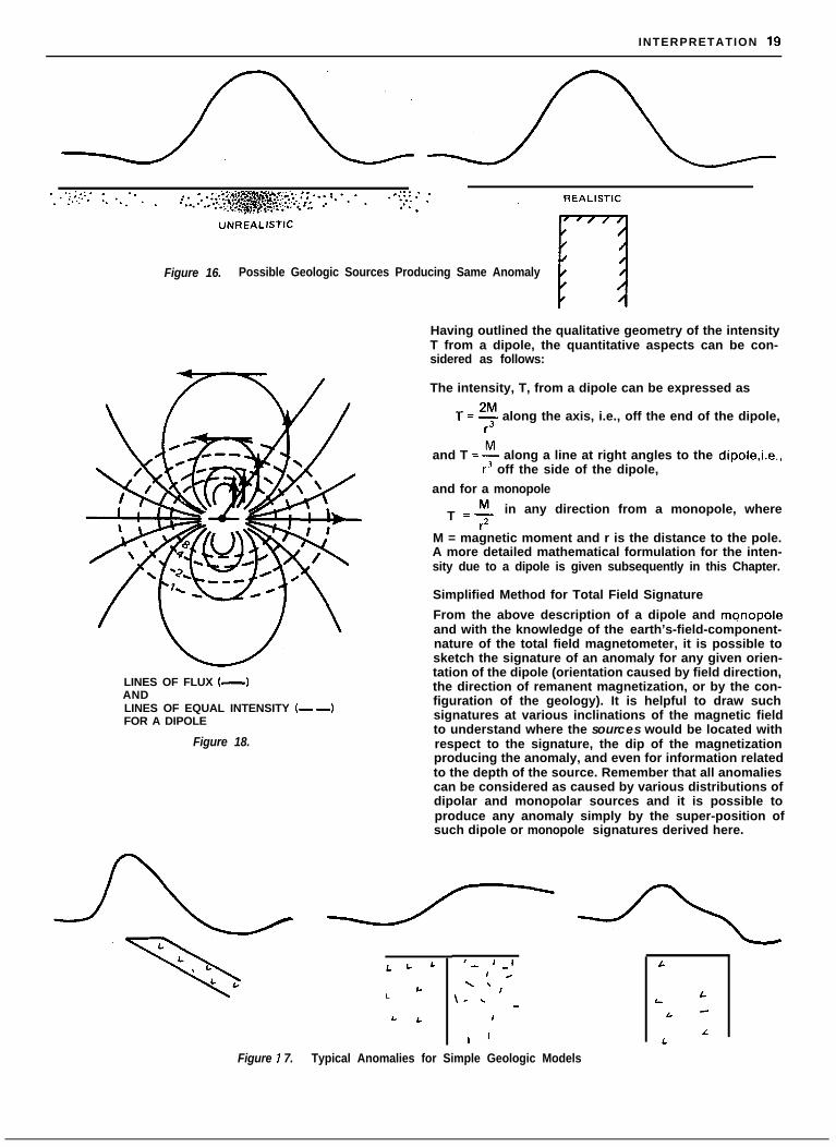
As was stated, in any potential field method the givenmagnetic signature can be produced by an infinite com-bination of sources so that there is no unique interpreta-tion. For example, the same anomaly could be producedby the peculiar distribution of magnetite (unrealisticgeologically), and a uniform distribution of magnetitewithin the prismatic form (realistic), both of which areshown in Figure 76. It must be emphasized that not onlyare simplifications required, but a reasonable geologicframework must be used as a guide when consideringthe various possible sources. A typical set of anomaly sig-natures of various sources might appear as in Figure 77.
Elementary Dipoles and MonopolesSince anomalies are explained herein in term of variousarrays of dipoles and monopoles, it is important to exam-ine their geometry and intensity characteristics. A mag-netic dipole produces a field with imaginary lines of fluxas shown in Figure 78. The intensity of the field, whichis proportional to the density of the flux lines is drawnas lines of equal intensity to express this relationship.From Figure 78, notice that 1) the intensity of the dipoleis twice as large off the ends of the dipole as it is at thesame distance off the side of the dipole. This explains,for example, why the earth’s magnetic field is approxi-mately 30,000 gammas at the magnetic equator and60,000 gammas at its poles; 2) the direction of the fieldoff the side of the dipole is parallel to the dipole itself,but opposite in sense; 3) the direction of the tangent ofthe field lines of a dipole are parallel along any radialline from the dipole.
A monopole has field lines which point radially in or outfrom the positive or negative monopole respectively. Theintensity is constant at a given distance and any directionfrom a monopole. In actual fact, there are no magneticmonopoles, but only dipoles whose ends are far apart.For all practical purposes, however, monopoles exist interms of the distance to the source and such geologicalconfiguration as shown in Figure 73.
Jijjijs f+I 4
ANTICLINE\J) ( M O D E L ) ORE BODY GRABEN (VOID)
Figure 15. Geological Model Representations of Common Magnetic Anomaly Sources
INTERPRETATION 19
99Figure 16. Possible Geologic Sources Producing Same Anomaly
n
Having outlined the qualitative geometry of the intensityT from a dipole, the quantitative aspects can be con-sidered as follows:
The intensity, T, from a dipole can be expressed as
T2!r3
along the axis, i.e., off the end of the dipole,
and T =E along a line at right angles to the dipole,i.e.,r3 off the side of the dipole,
and for a monopole
T =$- in any direction from a monopole, where
M = magnetic moment and r is the distance to the pole.A more detailed mathematical formulation for the inten-sity due to a dipole is given subsequently in this Chapter.
LINES OF FLUX (-4ANDLINES OF EQUAL INTENSITY I- -_)FOR A DIPOLE
Figure 18.
Figure 7 7. Typical Anomalies for Simple Geologic Models
Simplified Method for Total Field Signature
From the above description of a dipole and monopoleand with the knowledge of the earth’s-field-component-nature of the total field magnetometer, it is possible tosketch the signature of an anomaly for any given orien-tation of the dipole (orientation caused by field direction,the direction of remanent magnetization, or by the con-figuration of the geology). It is helpful to draw suchsignatures at various inclinations of the magnetic fieldto understand where the sources would be located withrespect to the signature, the dip of the magnetizationproducing the anomaly, and even for information relatedto the depth of the source. Remember that all anomaliescan be considered as caused by various distributions ofdipolar and monopolar sources and it is possible toproduce any anomaly simply by the super-position ofsuch dipole or monopole signatures derived here.
LL L
&L
L ‘
I- ‘_I
1 .\ \
\ - .I_I
I ’
L
LL
L -
‘‘
20 APPLICATIONS MANUAL FOR PORTABLE MAGNETOMETERS
DIPOLES
DIPOLES
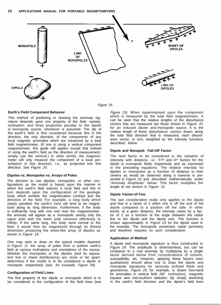
Figure 19.
Earth’s Field Component Behavior
This method of predicting or drawing the anomaly sig-nature depends upon one property of the field, namely,inclination, and three properties peculiar to the dipoleor monopole source, whichever is assumed. The dip ofthe earth’s field is first considered because this is thedirection, the only direction, of the components of anylocal magnetic anomalies which are measured by a totalfield magnetometer. (If one is using a vertical componentmagnetometer, this guide still applies except that insteadof using the earth’s field as the direction of measurement,simply use the vertical.) In other words, the magneto-meter will only measure the component of a local per-turbation in this direction, i.e., as projected into thisdirection. See Figure 20.
Dipoles vs. Monopoles vs. Arrays of Poles
The decision to use dipoles, monopoles, or other con-figurations as the model is based upon the manner inwhich the earth’s field induces a local field and this inturn depends upon the configuration of the geologicbody which exhibits the magnetization contrast and thedirection of the field. For example, a long body whichnearly parallels the earth’s field will tend to be magne-tized along its long dimension. Furthermore, if the bodyis sufficiently long with one end near the magnetometer,the anomaly will appear as a monopole seeing only theupper pole with the lower pole removed effectively toinfinity. If the same long, thin body were normal to thefield, it would then be magnetized through its thinestdimension producing the sheet-like array of dipoles asshown in Figure 19.
One may wish to draw on the typical models depictedin Figure 15, the array of poles from a uniform earth’sfield at various inclinations and orientations of the source.Whether the monopoles or the dipoles (and its equiva-lent line or sheet distributions) are close or far apart,determines if the model is to be considered a dipole ormonopole, respectively (see, for example, Figure 34).
Configuration of Field Lines
The first property of the dipole or monopole which is tobe considered is the configuration of the field lines (see
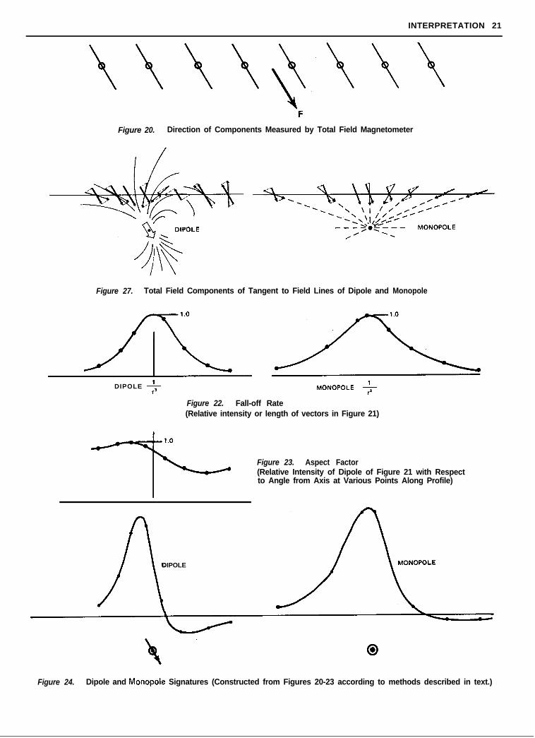
Figure 13). When superimposed upon the componentwhich is measured by the total field magnetometer, itcan be seen that the relative lengths of the disturbancevectors that are measured are those shown in Figure 21for an induced dipole and monopole source. It is therelative length of these disturbance vectors drawn alongthe total field direction that is measured, each disturb-ance vector, in turn, weighted by the intensity functionsdescribed below.
Dipole and Monopole Fall-Off Factor
The next factor to be considered is the variation ofintensity with distance, i.e., l/r3 and l/r* factors for thedipole or monopole fields respectively and as expressedin the preceding equations. The relative intensity fordipoles or monopoles as a function of distance to theircenters as would be observed along a traverse is pre-sented in Figure 22 and described mathematically under“Anomaly Amplitude” below. This factor multiplies thelength of net vectors in Figure 21.
Dipole Factor-of-Two
The last consideration really only applies to the dipoleand that is a factor of 2 when one is off the end of thedipole compared to a position off the side. In otherwords, at a given distance, the intensity varies by a fac-tor of 2 as a function of the angle between the radialline to the dipole and the dipole axis. This function isshown approximately in Figure 23 for the dipole used inthe example. The monopole possesses radial symmetryand therefore requires no such consideration.
Application of Method
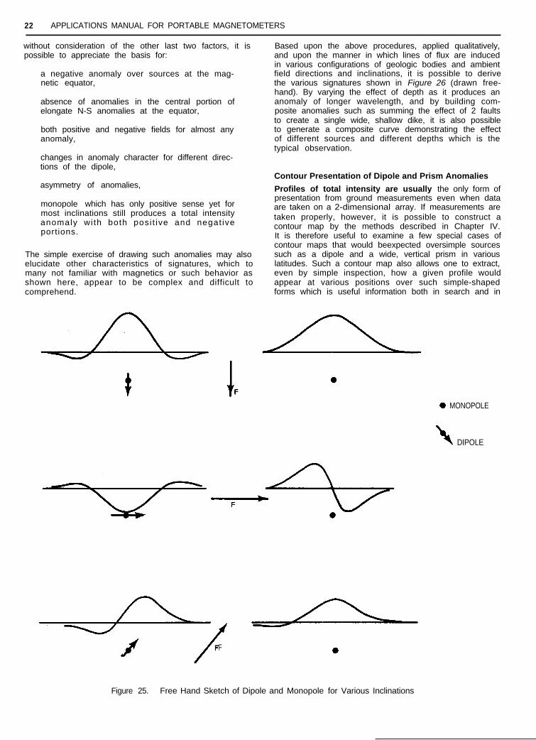
A dipole and monopole signature is thus constructed inFigure 24. The amplitude is dimensionless, but can becompared to a real anomaly by multiplying by a singlefactor derived below from considerations of volume,susceptibility, etc. However, applying these factors evenqualitatively should allow one to draw the dipole andmonopole signatures for variously inclined fields andgeometries. Figure 25, for example, is drawn free-handfor anomalies in vertical field (90° inclination), magneticequator and mid-southern latitudes. By simply sketchingin the earth’s field direction and the dipole’s field lines
INTERPRETATION 21
Figure 20. Direction of Components Measured by Total Field Magnetometer
Figure 27. Total Field Components of Tangent to Field Lines of Dipole and Monopole
rrDIPOLE + MONOPOLE +
Figure 22. Fall-off Rate(Relative intensity or length of vectors in Figure 21)
+
Figure 23. Aspect Factor(Relative Intensity of Dipole of Figure 21 with Respectto Angle from Axis at Various Points Along Profile)
ADIPOLE
Figure 24. Dipole and Monopole Signatures (Constructed from Figures 20-23 according to methods described in text.)
22 APPLICATIONS MANUAL FOR PORTABLE MAGNETOMETERS
without consideration of the other last two factors, it ispossible to appreciate the basis for:
a negative anomaly over sources at the mag-netic equator,
absence of anomalies in the central portion ofelongate N-S anomalies at the equator,
both positive and negative fields for almost anyanomaly,
changes in anomaly character for different direc-tions of the dipole,
asymmetry of anomalies,
monopole which has only positive sense yet formost inclinations still produces a total intensityanomaly wi th both posi t ive and negat iveportions.
The simple exercise of drawing such anomalies may alsoelucidate other characteristics of signatures, which tomany not familiar with magnetics or such behavior asshown here, appear to be complex and difficult tocomprehend.
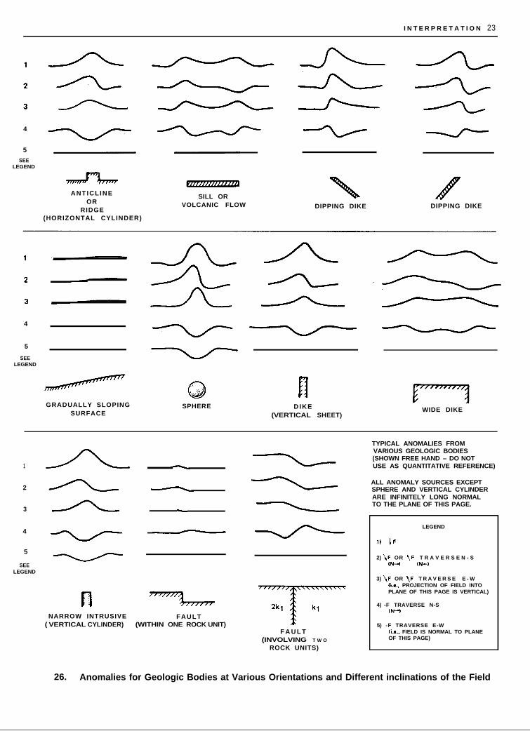
Based upon the above procedures, applied qualitatively,and upon the manner in which lines of flux are inducedin various configurations of geologic bodies and ambientfield directions and inclinations, it is possible to derivethe various signatures shown in Figure 26 (drawn free-hand). By varying the effect of depth as it produces ananomaly of longer wavelength, and by building com-posite anomalies such as summing the effect of 2 faultsto create a single wide, shallow dike, it is also possibleto generate a composite curve demonstrating the effectof different sources and different depths which is thetypical observation.
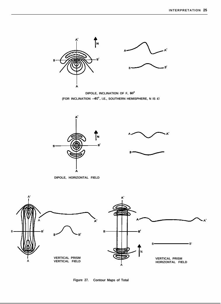
Contour Presentation of Dipole and Prism Anomalies
Profiles of total intensity are usually the only form ofpresentation from ground measurements even when dataare taken on a 2-dimensional array. If measurements aretaken properly, however, it is possible to construct acontour map by the methods described in Chapter IV.It is therefore useful to examine a few special cases ofcontour maps that would beexpected oversimple sourcessuch as a dipole and a wide, vertical prism in variouslatitudes. Such a contour map also allows one to extract,even by simple inspection, how a given profile wouldappear at various positions over such simple-shapedforms which is useful information both in search and in
0 MONOPOLE
‘G DIPOLE
-7 7f F a
Figure 25. Free Hand Sketch of Dipole and Monopole for Various Inclinations
I N T E R P R E T A T I O N 23
4
5
SEELEGEND
ANTICLINEOR
RIDGE(HORIZONTAL CYLINDER)
SILL ORVOLCANIC FLOW
\DIPPING DIKE
/DIPPING DIKE
4
5
SEELEGEND
GRADUALLY SLOPINGSURFACE
SPHERE
RDIKE
(VERTICAL SHEET)WIDE DIKE
1
2
3
4
5
SEELEGEND
t
riNARROW INTRUSIVE FAULT
( VERTICAL CYLINDER) (WITHIN ONE ROCK UNIT)F A U L T
(INVOLVING T W O
ROCK UNITS)
TYPICAL ANOMALIES FROMVARIOUS GEOLOGIC BODIES(SHOWN FREE HAND - DO NOTUSE AS QUANTITATIVE REFERENCE)
ALL ANOMALY SOURCES EXCEPTSPHERE AND VERTICAL CYLINDERARE INFINITELY LONG NORMALTO THE PLANE OF THIS PAGE.
LEGEND
2) IF OR tF T R A V E R S E N - SIN4 (N-b
3) \F OR \F T R A V E R S E E - W(i.e., PROJECTION OF FIELD INTOPLANE OF THIS PAGE IS VERTICAL)
4) -F TRAVERSE N-SIN-I
5) -F TRAVERSE E-W(i.e., FIELD IS NORMAL TO PLANEOF THIS PAGE)
Figure 26. Anomalies for Geologic Bodies at Various Orientations and Different inclinations of the Field
24 APPLICATIONS MANUAL FOR PORTABLE MAGNETOMETERS
geological exploration. Contour maps and selectedprofiles drawn across the anomaly are sketched inFigure 27.
Anomaly Amplitude
Amplitude Estimates for Common Sources
The large amplitude commonly observed anomalies(several hundred gammas or larger) are almost alwaysthe result of a large magnetization contrast, i.e., changein lithology where one igneous rock is in juxtapositionwith another or with a sedimentary or metamorphicrock of much lower susceptibility. It must be rememberedthat magnetization of common rocks varies over 6 ordersof magnitude. Anomalies due to structure alone, i.e.,varying configuration of a uniformly magnetized rock, sel-dom produces anomalies larger than 10 or 100 gammas.
The relative amplitude of a given anomaly (signature)has been shown to be a function of the earth’s fielddirection, the configuration of the source and the rem-anent magnetization if any. The maximum amplitude ofan anomaly is, on the other hand, largely a function ofthe depth and the contrast in the mass of magnetite (oriron, etc. in the case of search), and to a lesser extent,the configuration of the source. It is of interest to beable to estimate the maximum amplitude for a givensource in order to ‘model’ it for the sake of interpreta-tion. This estimated amplitude can be used with thenormalized, i.e., dimensionless, anomaly signaturesabove and in Figure 26 to produce the anomaly onewishes for comparison with the observed. Estimation ofthe maximum anomaly amplitude is also useful in plan-ning a survey or planning the grid and coverage neces-sary in search applications.
For a few generalized configurations, it is relativelysimple to estimate the maximum anomaly amplitude(at a single point above the source) assuming a depth,susceptibility and much simplified shape of the source.Expressions are given in the literature for calculation ofanomalies of more complex figures and later in thissection the calculation of the complete signature, i.e.,the amplitude as a function of distance along the pro-file for a few simple forms. The methods describedherein are merely order-of-magnitude techniques, butare useful for the applications covered by the Manual.
Estimation of the maximum anomaly for comparisonwith a given source requires first that the signature bestudied for the nature of the source; namely, whetherthe source can be approximated as an isolated dipole,monopole, or line or sheet-like array of such. In thecase of the latter two, adjacent traverses or a contourmap may be required to determine if it is 2-dimensional,i.e., very long normal to the traverse. A depth is thenassumed or crudely estimated (according to proceduresthat follow). In addition, the susceptibility is assumedor if source rocks are accessible, it is measured follow-ing methods outlined in Chapter VI. The formulae belowcan then be used remembering that they are basedupon simplifications and assumptions and are often nobetter than a factor of two.
The basic expression for estimating the maximumamplitude of any anomaly is
T=:
where T is the anomaly, M the magnetic moment, r thedistance (depth) to the source, and n a measure of the
rate of decay with distance, or fall-off rate (n = 3 for adipole, n = 2 or a monopole, etc.).
Since the magnetic moment M (and k) is usually givenin centimeter-gram-second (cgs) units, r must be incentimeters, n is dimensionless and T is in gauss. Toexpress T in gammas, multiply M by 105; if r is in feet,multiply r by 30 and raise the quantity 30r to the expo-nent n, e.g., if the source is a dipole, then n = 3, and if
say, r = 2 feet, M = 1000 cgs,
then T = 1000 x 10s(2 x 30)3
= 460 gammas.
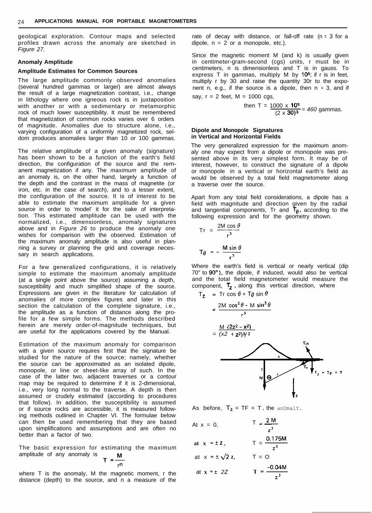
Dipole and Monopole Signaturesin Vertical and Horizontal Fields
The very generalized expression for the maximum anom-aly one may expect from a dipole or monopole was pre-sented above in its very simplest form. It may be ofinterest, however, to construct the signature of a dipoleor monopole in a vertical or horizontal earth’s field aswould be observed by a total field magnetometer alonga traverse over the source.
Apart from any total field considerations, a dipole has afield with magnitude and direction given by the radialand tangential components, Tr and To, according to thefollowing expression and for the geometry shown.
2M cos 0Tr = -
r3
Where the earth’s field is vertical or nearly vertical (dip70” to go”), the dipole, if induced, would also be verticaland the total field magnetometer would measure thecomponent, T, , along this vertical direction, where
TZ = Tr cos 6 + To sin 6
= 2M cos*e - M sinZf3
r3
M (222 - x2)= (x2 + Z2)5/2
T0
=TF=T
As before, T, = TF = T, the anOmalY.
At x = 0, T =?&23
0.175Mat x = +Z, T =
Z3
at x = *J2z, T = O
at x = * 2ZT = -0.04M
Z3
INTERPRETATION 25
DIPOLE, INCLINATION OF F, SO”
(FOR INCLINATION -SO”, I.E., SOUTHERN HEMISPHERE, N IS S)
DIPOLE, HORIZONTAL FIELD
A’
I
B
I VERTICAL PRISMA VERTICAL FIELD
B B’
VERTICAL PRISM1 HORIZONTAL FIELDA
Figure 27. Contour Maps of Total Intensity
26 APPLICATIONS MANUAL FOR PORTABLE MAGNETOMETERS
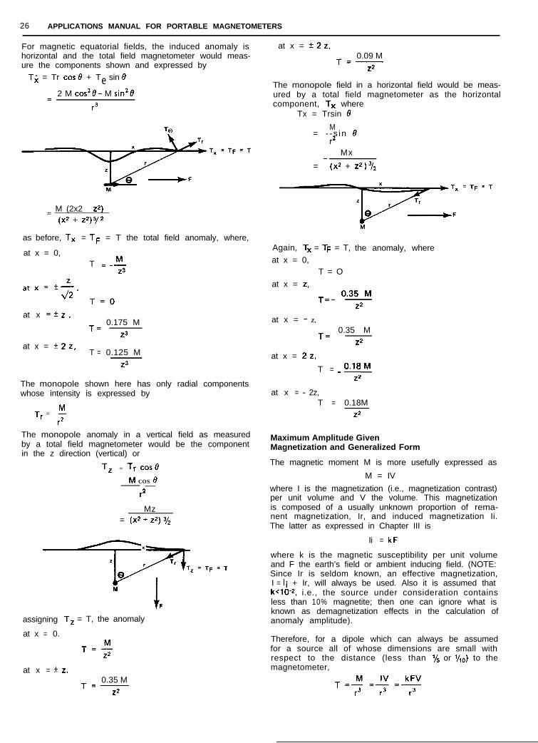
For magnetic equatorial fields, the induced anomaly ishorizontal and the total field magnetometer would meas-ure the components shown and expressed by
Tx = Tr cost!7 + Te sin 19
2 M cos’0 - M sin28=r3
=Tx=~~=~
M
= M (2x2 - 22)(x2 + z2) 5/2
as before, TX = TF = T the total field anomaly, where,
at x = 0,T = -s
atx=*$, T=O
at x = fz,T = 0.175 M
23
at x = +2Z,T = 0.125 M
23
The monopole shown here has only radial componentswhose intensity is expressed by
T, = !!!r*
The monopole anomaly in a vertical field as measuredby a total field magnetometer would be the componentin the z direction (vertical) or
TZ = Tr cost9
M COS 6=-
r2
Mz= (x2 + 22) y2
--T=TF=T
M
F
assigning T, = T, the anomaly
at x = 0.
T=$
at x = +-Z.0.35 MT=-
22
at x = *2z,0.09 MT=-
22
The monopole field in a horizontal field would be meas-ured by a total field magnetometer as the horizontalcomponent, TX where
Tx = Trsin 0
M= - - s in 8
r*Mx
= - (x2 + z2)%
)T, =TF=T
Again, TX = TF = T,
at x = 0,T = O
at x = z,
Y8 -F
M
the anomaly, where
T = _ o-35 M22
at x = - Z,
T = 0.35 M
22
at x = 2z,
T = _‘*18 M22
at x = - 2z,T = 0.18M
22
Maximum Amplitude GivenMagnetization and Generalized Form
The magnetic moment M is more usefully expressed as
M = IV
where I is the magnetization (i.e., magnetization contrast)per unit volume and V the volume. This magnetizationis composed of a usually unknown proportion of rema-nent magnetization, Ir, and induced magnetization Ii.The latter as expressed in Chapter III is
Ii = kF
where k is the magnetic susceptibility per unit volumeand F the earth’s field or ambient inducing field. (NOTE:Since Ir is seldom known, an effective magnetization,I = Ii + Ir, will always be used. Also it is assumed thatk<lO-2, i.e., the source under consideration containsless than 10% magnetite; then one can ignore what isknown as demagnetization effects in the calculation ofanomaly amplitude).
Therefore, for a dipole which can always be assumedfor a source all of whose dimensions are small withrespect to the distance (less than l/s or &) to themagnetometer,
kFVT=M=IV=---r3 r3 r3

INTERPRETATION 2 7
If the source is approximately spherical, then
T =kF (-$ nR3)
r3
For the same ore body in an equatorial field where F= 30,000 gammas and the induced dipole is now observedat a point on a line normal to the axis (no factor of 2)
where R is the radius of the source as in figure 28 T = - 3.6 gammas
If the measurement is made along the axis of the dipole(see Figure 29), then
T =2kF (,+ nap)
r3
T=r ’ SUSCEPTIBILITY, k
- F
Figure 28. Anomaly of Sphere in Horizontal Field
T=r3 SUSCEPTIBILITY, k
Figure 29. IAnomaly of Sphere in Vertical Field VF
As an example, consider an ore body 100 feet wide(R = 50), 500 feet deep comprised of 10% magnetite(k = 0.3), in a steeply dipping field (SO” to 90” latitude)in a field of 60,000 gammas:
T = 2 (0.10 X 0.3) X 6 X lo4 (F)(&)’ = 14.4 gammas
kF nR’T - -
r’
t
= nR’
F
Thus a given dipolar source in an equatorial field willhave only l/4 the maximum anomaly amplitude it wouldhave in a polar region.
The above expressions are usually valid only for suchsources as a small distant ore body (containing magne-tite), small structure in deep basement, or most objectsinvolved in search applications (see Chapter VII). Themagnetization is expressed in gauss or gammas asdesired. Since the anomalies are also expressed in termsof magnetic units, it follows that the units of dimensionin the numerator must be of the same order as thedenominator since they must cancel. Therefore, for a
dipole whose anomaly varies as 1 (said to have a fall-r3
off of 1 ), the volume, V, has dimensions of R3. In ther.’
case of a monopole, which varies as 1 , the magneticr*
moment, M, is equal to IA where A is surface area andhas dimensions of R*. Consider for example, a verticalbasement intrusive in a polar region with an upper sur-face 1000 feet in diameter at a depth of 5000 feet, witha susceptibility contrast of 1 O-2 in a field of 60,000 gammas.Thus,
kF nR*T =-=r*
lo-’ X 6X lo4 X TI 18 gammas.
Horizontal prisms or cylinders also vary as -!- , withr*
magnetic moment M equal to 21A (IA for E-W horizontalprisms in equatorial regions) where A is the cross-sec-tional area of the prism (see figure 30). (NOTE: The
long horizontal prism varies as 1 not because it appearsR2
to be comprised of a monopole, but because it is a lineof dipoles (in steeply dipping fields) and the effect ofadjacent dipoles along an infinitely long line is ‘seen’more by the magnetometer at a distant point of measure-ment than if all the magnetization were concentrated ata point as in an isolated dipole).
(NOTE: ALSO VALID FOR END OF N-S HORIZONTALCYLINDER IN HORIZONTAL FIELD)
(NOTE:
2kF nR’T-
r’
ALSO VALID FOR E-W HORIZONTAL CYLINDERIN HORIZONTAL FIELD)
Figure 30. Anomaly of Vertical and Horizontal Cylinders

28 APPLICATIONS MANUAL FOR PORTABLE MAGNETOMETERS
A narrow, vertical dike in steep field or the edge of ahorizontal sheet in a horizontal field can be consideredas a line of monopoles varying as l/r which is a lowerrate of fall-off than a singl e monopo e for the samereasons given above for a horizontal cylinder (see Fig-ure 37). The magnetic moment M = It where t = width ofdike. Since the anomaly varies as l/r, the dimensionsof t are simply length. As an example, a vertical dikemight be 100 feet wide, at a depth of 500 feet, withk = 10-3 in a field of 50,000 gammas, or
kft lO-.j x 5 x lo4 x 10’T =-= = 10 gammasr 5 x 10’
kFtT=-
r
WHERE ttr
Figure 31. Anomaly of Narrow Vertical Dike
A common point of ambiguity arises with such simplifiedschemes as these in the case of a dike which is nearlyas wide as it is deep. In this case, the anomaly is approxi-mated as something between a line of monopoles asabove and a sheet of monopoles as shown in the follow-ing. Moreover, as the dike is even wider than its depth,it can be approximated simply by 2 faulted contacts with‘no anomaly’ in between.
For a semi-infinite slab of material such as a rock sur-face of great thickness and breadth in a non-horizontalfield, the flux lines do not vary in direction or densityabove the slab, therefore the field does not vary at allwith distance to its surface (similar to the limit of thespherical dipole above where R = r) so that
M 2711T Z-Zr0
-, or T = 27r kF1
which is useful in estimating the magnitude of the anom-aly at a vertical fault (see Figure 32). For example, con-sider two rock types at a vertical contact of k = lo-9 andk = 10-S for an effective susceptibility contrast of k = 10-3(10-5 E3 0 relative to 10-s) and whe re F = 50,000 gammas.Thus
T = 27rX 10e3 X 5 X lo4 = 300 g a m m a s
If the rocks had k = 10-4 and 10-3, the effective suscepti-bility contrast would be
IO-” _ 10-J = 1 0 X 1O-4 - 1O-4 = 9X 10e4 a n d
T = 277 X 9 X lO-4 X 5 X lo4 = 270gammas
This simple example of two adjacent rock types is prob-ably applicable in more instances in interpretation thanany of the other geometries discussed above.
T = 2nkF
I
Figure 32. Anomaly of Semi-infinite Slab
Anomaly Depth Characteristics
In a very approximate fashion, the wavelength, or, effec-tive width (or ‘half-width’ described in the following) ofthe anomaly and, with more accuracy, the width of cer-tain characteristics of the anomaly such as slope, aremeasures of the depth to its source. However, recogni-tion of the anomaly, the anomaly ‘zero’ and certain slopeswould not only appear as different values as determinedby different interpreters, but they also depend uponwhat is removed as the regional gradient. More objec-tive criteria are used in some cases such as the nearlystraight portions of a slope, and distances and anglesbetween inflection points, peak values and other anomalycharacteristics.
Anomaly Width
In general, the anomaly width as shown i n Figure 33 ison the order of 1 to perhaps 3 times the depth. Thus,when an anomaly appears to have a width as such of100 feet, it is definitely not produced by a source at1000 feet or at 10 feet, but more likely by a source be-tween 30 and 100 feet deep (or distant). Such criteria,approximate as it is, is nevertheless useful for cursoryinterpretation of profiles and maps.
Anomaly Depth Estimation
Much is written on the variety and relative merit of meth-ods for estimating the depth to the source of anomalies.Since the magnetometer is primarily a tool for subsur-face mapping and detection, it follows that determinationof the depth as well as edges of bodies is important inits application to geological exploration and search. Thebasis for depth determination is presented here in briefwhich, together with the foregoing background on anom-aly behavior, should allow one to at least appreciatehow a variation in depth affects an anomaly. In mostcases, one needs only to apply this knowledge quali-tatively through visual inspection of a profile. Whateverthe requirement, depths may be estimated by visualinspection, several rules of thumb, modeling (i.e., calcu-lation of assumed source and comparison with observed),measured gradient techniques (see Chapter VIII), orvarious computer-oriented procedures. As was demon-strated earlier, a given anomaly could have an infinitenumber of possible sources and source depths, but therealistic models that are assumed usually produce maxi-mum depth estimates.
Knowledge of the depth of a particular formation orsource may have considerable geological significanceas it determines the nature oconfiguration of a fo-ma-forma-
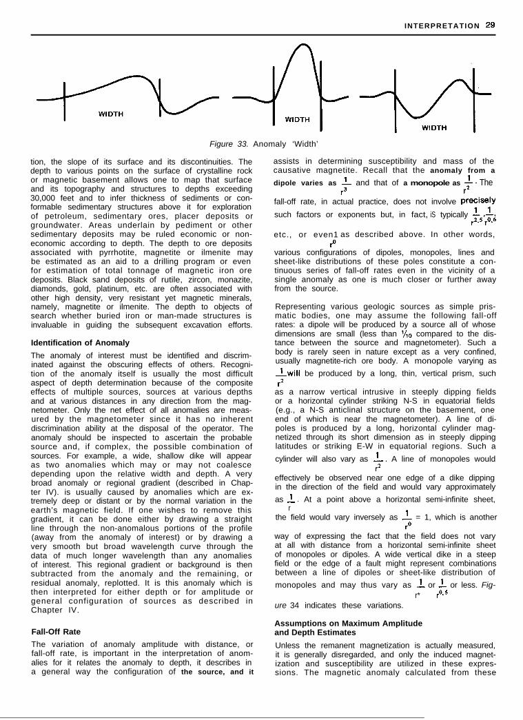
INTERPRETATION 29
Figure 33. Anomaly ‘Width’
tion, the slope of its surface and its discontinuities. Thedepth to various points on the surface of crystalline rockor magnetic basement allows one to map that surfaceand its topography and structures to depths exceeding30,000 feet and to infer thickness of sediments or con-formable sedimentary structures above it for explorationof petroleum, sedimentary ores, placer deposits orgroundwater. Areas underlain by pediment or othersedimentary deposits may be ruled economic or non-economic according to depth. The depth to ore depositsassociated with pyrrhotite, magnetite or ilmenite maybe estimated as an aid to a drilling program or evenfor estimation of total tonnage of magnetic iron oredeposits. Black sand deposits of rutile, zircon, monazite,diamonds, gold, platinum, etc. are often associated withother high density, very resistant yet magnetic minerals,namely, magnetite or ilmenite. The depth to objects ofsearch whether buried iron or man-made structures isinvaluable in guiding the subsequent excavation efforts.
Identification of Anomaly
The anomaly of interest must be identified and discrim-inated against the obscuring effects of others. Recogni-tion of the anomaly itself is usually the most difficultaspect of depth determination because of the compositeeffects of multiple sources, sources at various depthsand at various distances in any direction from the mag-netometer. Only the net effect of all anomalies are meas-ured by the magnetometer since it has no inherentdiscrimination ability at the disposal of the operator. Theanomaly should be inspected to ascertain the probablesource and, if complex, the possible combination ofsources. For example, a wide, shallow dike will appearas two anomalies which may or may not coalescedepending upon the relative width and depth. A verybroad anomaly or regional gradient (described in Chap-ter IV). is usually caused by anomalies which are ex-tremely deep or distant or by the normal variation in theearth’s magnetic field. If one wishes to remove thisgradient, it can be done either by drawing a straightline through the non-anomalous portions of the profile(away from the anomaly of interest) or by drawing avery smooth but broad wavelength curve through thedata of much longer wavelength than any anomaliesof interest. This regional gradient or background is thensubtracted from the anomaly and the remaining, orresidual anomaly, replotted. It is this anomaly which isthen interpreted for either depth or for amplitude orgeneral configuration of sources as described inChapter IV.
Fall-Off Rate
The variation of anomaly amplitude with distance, orfall-off rate, is important in the interpretation of anom-alies for it relates the anomaly to depth, it describes ina general way the configuration of the source, and it
assists in determining susceptibility and mass of thecausative magnetite. Recall that the anomaly from a
dipole varies as 1 and that of a monopole as r+ . Ther3
fall-off rate, in actual practice, does not involve PreCiSelY
such factors or exponents but, in fact, iS typically +5&r’ r*
etc., or even1 as described above. In other words,r”
various configurations of dipoles, monopoles, lines andsheet-like distributions of these poles constitute a con-tinuous series of fall-off rates even in the vicinity of asingle anomaly as one is much closer or further awayfrom the source.
Representing various geologic sources as simple pris-matic bodies, one may assume the following fall-offrates: a dipole will be produced by a source all of whosedimensions are small (less than 1/,o compared to the dis-tance between the source and magnetometer). Such abody is rarely seen in nature except as a very confined,usually magnetite-rich ore body. A monopole varying as
_!_will be produced by a long, thin, vertical prism, suchr*
as a narrow vertical intrusive in steeply dipping fieldsor a horizontal cylinder striking N-S in equatorial fields(e.g., a N-S anticlinal structure on the basement, oneend of which is near the magnetometer). A line of di-poles is produced by a long, horizontal cylinder mag-netized through its short dimension as in steeply dippinglatitudes or striking E-W in equatorial regions. Such a
cylinder will also vary as _!_ . A line of monopoles wouldr*
effectively be observed near one edge of a dike dippingin the direction of the field and would vary approximately
as 1 . At a point above a horizontal semi-infinite sheet,r
the field would vary inversely as _!_ = 1, which is anotherr”
way of expressing the fact that the field does not varyat all with distance from a horizontal semi-infinite sheetof monopoles or dipoles. A wide vertical dike in a steepfield or the edge of a fault might represent combinationsbetween a line of dipoles or sheet-like distribution of
monopoles and may thus vary as _!_ or 1 or less. Fig-r* ro. 5
ure 34 indicates these variations.
Assumptions on Maximum Amplitudeand Depth Estimates
Unless the remanent magnetization is actually measured,it is generally disregarded, and only the induced magnet-ization and susceptibility are utilized in these expres-sions. The magnetic anomaly calculated from these
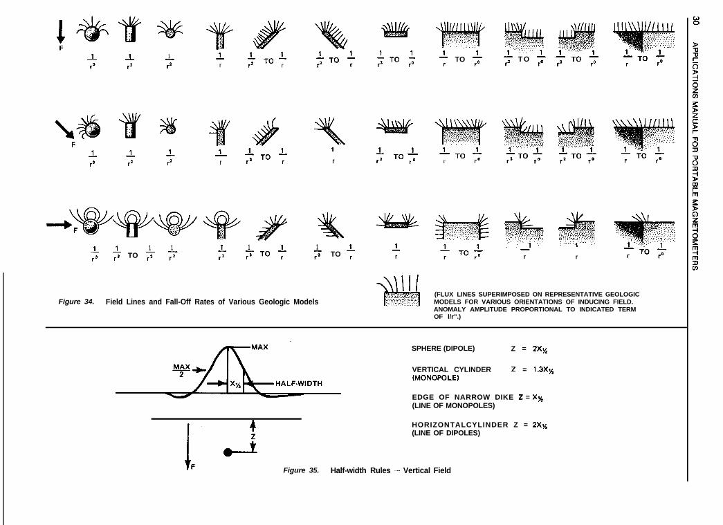
81 1r* To r
wI _% :-
5.0 $i- TO f
r1
r3
1r*
1-r3
1r
f T O
%‘:.
1 1 -1,p TO ,o
1 1r TO ror
%‘..
r
~ .~~ ~~. . ; ., :‘:;. : :.. ..’ : ‘,.. :.,:T..
..; .‘I. i . . _. ._._.. .:
: :.;
I”-‘.1 ”-r rf TO ro
1r 1 1 1 _I_ 1rs TO 7 T;-
i!_r3 rz T”-TO r
1 1F; TO r
1r
+!-IIIIdle:g..~..::,-::~~~~.~.,.::..:~~,..~..:.:.,.::~~~,.:.,,. . . . . .._. ..,.......‘..:::‘.:‘..‘:I:::‘;::::..,
(FLUX LINES SUPERIMPOSED ON REPRESENTATIVE GEOLOGICMODELS FOR VARIOUS ORIENTATIONS OF INDUCING FIELD.ANOMALY AMPLITUDE PROPORTIONAL TO INDICATED TERMOF l/r”.)
Figure 34. Field Lines and Fall-Off Rates of Various Geologic Models
SPHERE (DIPOLE) Z = 2Xx
VERTICAL CYLINDER(MONOPOLE)
2 = 1.3Xx
EDGE OF NARROW DIKE 2 = Xx(LINE OF MONOPOLES)
4 HORIZONTALCYLINDER Z = 2Xx
i
(LINE OF DIPOLES)
Figure 35. Half-width Rules - Vertical Field
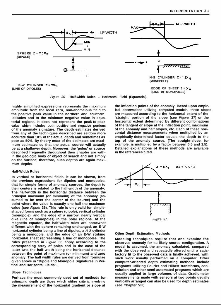
INTERPRETATION 3 1
~~~~ --G+II? LF-WIDTH
SPHERE Z = 2.5Xx(DIPOLE)
4-F
z
- F
E-W CYLINDER 2 = 2x3~(LINE OF DIPOLES)
N-S CYLINDER 2 = 1.3Xx(MONOPOLE)
EDGE OF SHEET Z = Xx(LINE 0F MONOPOLES)
Figure 36. Half-width Rules - Horizontal Field (Equatorial)
highly simplified expressions represents the maximumamplitude from the local zero, non-anomalous field tothe positive peak value in the northern and sourthernlatitudes and to the minimum negative value in equa-torial regions. It does not represent the peak-to-peakvalue which includes both positive and negative portionsof the anomaly signature. The depth estimates derivedfrom any of the techniques described are seldom moreaccurate than 10% of the actual depth and sometimes aspoor as 50%. By theory most of the estimates are maxi-mum estimates so that the actual source will actuallybe at a shallower depth. Moreover, the ‘poles’ or sourcedescribed frequently throughout their chapter are with-in the geologic body or object of search and not simplyon the surface; therefore, such depths are again maxi-mum depths.
Half-Width Rules
In vertical or horizontal fields, it can be shown, fromthe previous expressions for dipoles and monopoles,that for simple forms of anomaly sources, the depth totheir centers is related to the half-width of the anomaly.The half-width is the horizontal distance between theprincipal maximum (or minimum) of the anomaly (as-sumed to be over the center of the source) and thepoint where the value is exactly one-half the maximumvalue (see Figure 35). This rule is only valid for simple-shaped forms such as a sphere (dipole), vertical cylinder(monopole), and the edge of a narrow, nearly verticaldike (line of monopoles) in the polar regions. At themagnetic equator, the half-width rules are somewhatdifferent with the sphere remaining unchanged, an E-Whorizontal cylinder being a line of dipoles, a N-S cylinderbeing a monopole, and the edge of an E-W strikinghorizontal sheet representing a line of monopoles. Therules presented in Figure 36 apply according to thecorresponding array of poles and in the case of thelatter two, the half width being the horizontal distancebetween the point of maximum (or minimum) and zeroanomaly. The half width rules are derived from formulaegiven above in “Dipole and Monopole Signatures in Ver-tical and Horizontal Fields”.
Slope Techniques
Perhaps the most commonly used set of methods forestimating depth are those which utilize criteria involvingthe measurement of the horizontal gradient or slope at
the inflection points of the anomaly. Based upon empir-ical observations utilizing computed models, these slopesare measured according to the horizontal extent of the‘straight’ portion of the slope (see Figure 37) or thehorizontal extent determined by different combinationsof the tangent or slope at the inflection point, maximumof the anomaly and half slopes, etc. Each of these hori-zontal distance measurements when multiplied by anempirically-determined factor equals the depth to thetop of the anomaly source. (The straight-slope, forexample, is multiplied by a factor between 0.5 and 1.5).Detailed explanations of these methods are availablein the references cited.
,azl.5
Figure 37.
Other Depth Estimating Methods
Modeling techniques require that one examine theobserved anomaly for its likely source configuration. Amodel is assumed, the anomaly calculated, comparedwith the observed and repeatedly altered until a satis-factory fit to the observed data is finally achieved, withsuch work usually performed on a computer. Othercomputer-oriented depth estimating methods includeprograms utilizing Fourier and Hilbert transforms, con-volution and other semi-automated programs which areusually applied to large volumes of data. Gradiometermeasurements made with sensors at two points usuallyvertically arranged can also be used for depth estimates(see Chapter VIII).
32 APPLICATIONS MANUAL FOR PORTABLE MAGNETOMETERS
Interpretation Summary
Interpretation is facilitated if one can thoroughly familiar-ize himself with how and why a given source producesan anomaly in the earth’s field, the nature of total fieldmeasurements and the general behavior of an anomalysignature with increasing depth. What at first may haveappeared complex in the interpretation of field profilesand maps is more readily understood when the abovephenomena are examined one at a time.
The first procedure that should be followed in the inter-pretation of a given profile is to focus on the anomalywidth and shape and attempt to construct at least amental image of the source in realistic geologic terms(or object in the case of search) and its depth. Use theeye to discriminate against noise and the regional gra-dient or filter by one of the suggested techniques.Anomalous horizontal gradients should then be used,for lack of any other specific criteria, as an indicatorof the edge of subsurface structures producing a mag-netization contrast. Most anomalies on any given profileor map represent a simple contrast in magnetization orlithology. i.e., the edge of a body. Attempt to correlatesuch features on adjacent lines or interpret them ascontacts on a total intensity contour map. The cessation,
displacement or interruption of otherwise long or con-tinuous features may also represent significant geologicstructural information. However, one must realize alsothat a magnetic survey is only able to map a contactwhere there is a magnetization contrast so that, forexample, different lithologies on either side of a longcontinuous fault will be mapped only in segments wheresuch contrasts occur.
Changes in the character of the short wavelength anom-alies (noise) may also represent mappable informationif one is careful to evaluate their typical depth so as notto be mapping irrelevant soil anomalies. Negative anom-alies arising from features of locally lower magnetiza-tion are as important geologically as the more commonpositive anomalies. Furthermore, the most geologicallysignificant anomalies on a given map are probably themore subtle ones and not necessarily the largest, mostprominent anomalies. Lastly, the total intensity profilesand maps are not an end in themselves, but are renderedusable only when expressed in terms of geology (orobjects of a search). The more geological informationone has (or size, magnetic or depth information for anobject of search) the more valuable the total intensitydata becomes and vice-versa.
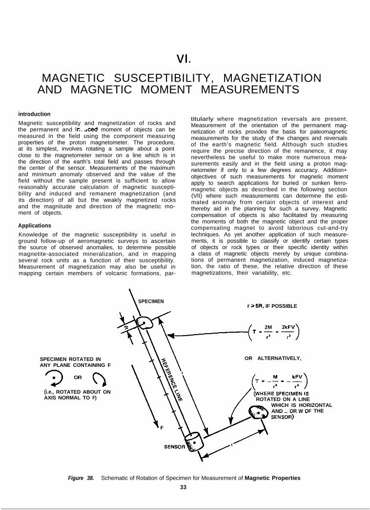
VI.
MAGNETIC SUSCEPTIBILITY, MAGNETIZATIONAND MAGNETIC MOMENT MEASUREMENTS
introduction
Magnetic susceptibility and magnetization of rocks andthe permanent and induced moment of objects can bemeasured in the field using the component measuringproperties of the proton magnetometer. The procedure,at its simplest, involves rotating a sample about a pointclose to the magnetometer sensor on a line which is inthe direction of the earth’s total field and passes throughthe center of the sensor. Measurements of the maximumand minimum anomaly observed and the value of thefield without the sample present is sufficient to allowreasonably accurate calculation of magnetic suscepti-bility and induced and remanent magnetization (andits direction) of all but the weakly magnetized rocksand the magnitude and direction of the magnetic mo-ment of objects.
Applications
Knowledge of the magnetic susceptibility is useful inground follow-up of aeromagnetic surveys to ascertainthe source of observed anomalies, to determine possiblemagnetite-associated mineralization, and in mappingseveral rock units as a function of their susceptibility.Measurement of magnetization may also be useful inmapping certain members of volcanic formations, par-
\SPECIMEN
titularly where magnetization reversals are present.Measurement of the orientation of the permanent mag-netization of rocks provides the basis for paleomagneticmeasurements for the study of the changes and reversalsof the earth’s magnetic field. Although such studiesrequire the precise direction of the remanence, it maynevertheless be useful to make more numerous mea-surements easily and in the field using a proton mag-netometer if only to a few degrees accuracy. Addition+objectives of such measurements for magnetic momentapply to search applications for buried or sunken ferro-magnetic objects as described in the following section(VII) where such measurements can determine the esti-mated anomaly from certain objects of interest andthereby aid in the planning for such a survey. Magneticcompensation of objects is also facilitated by measuringthe moments of both the magnetic object and the propercompensating magnet to avoid laborious cut-and-trytechniques. As yet another application of such measure-ments, it is possible to classify or identify certain typesof objects or rock types or their specific identity withina class of magnetic objects merely by unique combina-tions of permanent magnetization, induced magnetiza-tion, the ratio of these, the relative direction of thesemagnetizations, their variability, etc.
r 2- 5R. IF POSSIBLE
/_ 2M 2kFV)
SPECIMEN ROTATED IN OR ALTERNATIVELY,ANY PLANE CONTAINING F
7 OR Q(i.e., ROTATED ABOUT ONAXIS NORMAL TO F) ROTATED ON A LINE
WHICH IS HORIZONTALAND E OR W OF THE
Figure 38. Schematic of Rotation of Specimen for Measurement of Magnetic Properties
33
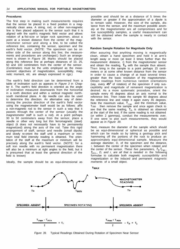
34 APPLICATIONS MANUAL FOR PORTABLE MAGNETOMETERS
Procedures
The first step in making such measurements requiresthat the sensor be placed in a fixed position in a mag-netically clean area. A string, rod, or other non-magneticline is then placed adjacent to the sensor such that it isaligned with the earth’s magnetic field vector and allowsrotation of a fist-size or larger rock specimen, about apoint at a known distance from the center of the mag-netometer sensor and along a line, to be called thereference line, containing the sensor, specimen and theearth’s field vector. (NOTE: The specimen can be oneither side of the sensor along this line; the measure-ments and procedures are unchanged.) Such an arrange-ment is shown in Figure 38. Marks should be placedalong this reference line at perhaps distances of 10, 25,50 and 100 centimeters from the center of the sensor.(Centimeters must be the units employed as the meas-urement objectives of magnetization, susceptibility, mag-netic moment, etc. are always expressed in cgs.)
The earth’s field direction can be determined from atable of inclination such as appears in Figure 3 in Chap-ter II. The earth’s field direction is oriented as the angleof inclination measured downwards from the horizontalin a north direction and within a vertical magnetic north-south meridional plane. A dip needle can also be usedto determine this direction. An alternative way of deter-mining the precise direction of the earth’s field vectorusing the magnetometer itself would be as follows: affixa non-magnetic rod to the sensor in such a way that itpasses through the center of the sensor (usually themagnetometer staff is such a rod). At a point perhaps30 to 50 centimeters away from the sensor, place aneedle or other very long but thin ferromagnetic (steel)object (it does not necessarily have to be permanentiymagnetized) along the axis of the rod. Take this rigidarrangement of staff, sensor and needle (small dipole)and slowly re-orient the staff until a maximum or mini-mum total field intensity reading is obtained. The orien-tation of the staff at the maximum or minimum will beprecisely along the earth’s field vector. (NOTE: for asoft iron needle with no permanent magnetization therewill also be a minimum at right angles to the field, but itis presumed that at least the general direction of thefield is known)
Ideally, the sample should be as equi-dimensional as
possible and should be at a distance of 5 times thediameter or greater if the approximation of a dipole isto remain valid. However, the size of the sample, dis-tance from the sensor, and the maximum possible anom-aly at the magnetometer are all compromises and forlow susceptibility samples, a useful measurement canstill be obtained when the sample is nearly in contactwith the sensor.
Random Sample Rotation for Magnitude Only
After assuring that anything moving is magneticallyclean, obtain a hand specimen and hold it at arm’slength away or more (at least 3 times further than themeasurement distance, r) from the magnetometer sensorand obtain the reading, T,,, with the sample thus absent.Then bring in the sample to a point perhaps 15 centi-meters or at some other known distance from the sensorin order to cause a change of at least several timesgreater than the basic resolution of the magnetometer.Obtain readings from numerous random orientations(say, every 45” of rotation) of the specimen if only sus-ceptibility and magnitude of remanent magnetization isdesired. As a more systematic procedure, orient thesample every 45 degrees about an axis normal to thereference line. Then rotate the sample 90 degrees aboutthe reference line and rotate it again every 45 degrees.Note the maximum value, T,,, and the minimum value,Tmm , then remove the sample and once again check tosee that the same reading, To, is obtained as observedat the start of the test. If the same reading is not obtained(or within 2 gammas), conduct the measurements over.If one were to plot such measurements, they wouldappear as in Figure 39.
Next, measure the diameter of the sample which shouldbe as equi-dimensional or spherical as possible andwhich can be made so by taking a geology pick andhammering off the portions of the rock to produce anapproximately equi-dimensional sample. Measure theaverage diameter, D, of the specimen and the distance,r, between the center of the specimen when rotated andthe center of the sensor. These five parameters, TO, T,,, ,Tmin 9 D, and r, are all that is needed in the followingformulae to calculate both magnetic susceptibility andmagnetization or the induced and permanent magneticmoments of a small object.
TMAX
A
To TMlN To
SPECIMEN ABSENT SPECIMEN ABSENT
Tmax - Tmin Tmax + Tmin= T,
2 2- To = Ti
Figure 39. Typical Readings Obtained During Rotation of Specimen Near Sensor
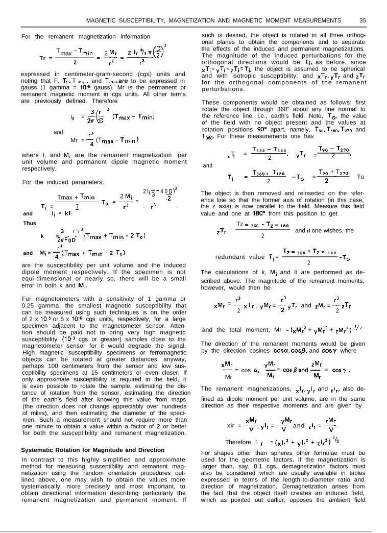
MAGNETIC SUSCEPTIBILITY, MAGNETIZATION AND MAGNETIC MOMENT MEASUREMENTS 35
For the remanent magnetization information
Tmax - Tmin 2 MrTr = c-z
2 Ir 4/3 7r(+)’
2 r3 r3
expressed in centimeter-gram-second (cgs) units andnoting that F, Tr , T ,,,,,, , and TmdXare to be expressed ingauss (1 gamma = 10-S gauss). Mr is the permanent orremanent magnetic moment in cgs units. All other termsare previously defined. Therefore
lr = $La 3 (Tmax- Tmin)0\
andMr = ; (Tmax - Tmin )
where I, and M, are the remanentunit volume and permanent dipolerespectively.
For the induced parameters,
magnetization permagnetic moment
Tmax + Tmin 2 Mi
Ti
2 1’277 4 0 D32
= -To =r3= - -7 r3and Ii = kF -
Thus3 r3
k = - -02nF D
(Tmax+Tmin_2To)
r3and Mi = q(Tmax + Tmin - 2 To)
are the susceptibility per unit volume and the induceddipole moment respectively. If the specimen is notequi-dimensional or nearly so, there will be a smallerror in both k and Mi.
For magnetometers with a sensitivity of 1 gamma or0.25 gamma, the smallest magnetic susceptibility thatcan be measured using such techniques is on the orderof 2 x 10⁻⁵ or 5 x 10-e cgs units, respectively, for a largespecimen adjacent to the magnetometer sensor. Atten-tion should be paid not to bring very high magneticsusceptibility (10-a cgs or greater) samples close to themagnetometer sensor for it would degrade the signal.High magnetic susceptibility specimens or ferromagneticobjects can be rotated at greater distances, anyway,perhaps 100 centimeters from the sensor and low sus-ceptibility specimens at 15 centimeters or even closer. Ifonly approximate susceptibility is required in the field, itis even possible to rotate the sample, estimating the dis-tance of rotation from the sensor, estimating the directionof the earth’s field after knowing this value from maps(the direction does not change appreciably over hundredsof miles), and then estimating the diameter of the speci-men. Such a measurement should not require more thanone minute to obtain a value within a factor of 2 or betterfor both the susceptibility and remanent magnetization.
Systematic Rotation for Magnitude and Direction
In contrast to this highly simplified and approximatemethod for measuring susceptibility and remanent mag-netization using the random orientation procedures out-lined above, one may wish to obtain the values moresystematically, more precisely and most important, toobtain directional information describing particularly theremanent magnetization and permanent moment. If
such is desired, the object is rotated in all three orthog-onal planes to obtain the components and to separatethe effects of the induced and permanent magnetizations.The magnitude of the induced perturbations for theorthogonal directions would be Ti, as before, sincexTi= yTi = zTi= Ti, the object is assumed to be sphericaland with isotropic susceptibility; and xTr, YTr and zTrfor the or thogonal components of the remanentperturbations.
These components would be obtained as follows: firstrotate the object through 360” about any line normal tothe reference line, i.e., earth’s field. Note, To, the valueof the field with no object present and the values atrotation positions 90” apart, namely, TgO, TIBO, T2r0 andT360. For these measurements one has
T TT =
1 8 0 - 3 6 0 T9 0 - T270
x r 2 ’ yTr = 2 1
and
Ti =T360 + Ttso T90 +T270
2-To = 2 - To
The object is then removed and reinserted on the refer-ence line so that the former axis of rotation (in this case,the z axis) is now parallel to the field. Measure this fieldvalue and one at 180’ from this position to get
Tz = 360 -Tz= 180
zTr =2
and if one wishes, the
redundant value Ti =Tz = 3 6 0 +Tz = 1 8 0
2-TO
The calculations of k, Mi and Ii are performed as de-scribed above. The magnitude of the remanent moments,however, would then be
xMr = 2r3 r3
2xTr , yMr = 1 yTr and ZMr = - ZTr
2
and the total moment, Mr = (xMr* + yM,* + zM,*) l/2
The direction of the remanent moments would be givenby the direction cosines cosa, co@, and cosy where
xMr Y”r zMr- = cos (Y,Mr
M= cosfland- = cosy.r Mr
The remanent magnetizations, xIr, Yl, and zl,, also de-
fined as dipole moment per unit volume, are in the samedirection as their respective moments and are given by
xMr Y”r zMrxlr = v, Ylr = 7 and zlr = -
V
Therefore I r = (xlr’ + Ylr* + zlr’) ‘12
For shapes other than spheres other formulae must beused for the geometric factors. If the magnetization islarger than, say, 0.1 cgs, demagnetization factors mustalso be considered which are usually available in tablesexpressed in terms of the length-to-diameter ratio anddirection of magnetization. Demagnetization arises fromthe fact that the object itself creates an induced field,which as pointed out earlier, opposes the ambient field
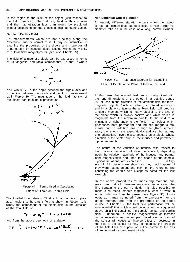
36 APPLICATIONS MANUAL FOR PORTABLE MAGNETOMETERS
in the region to the side of the object (with respect tothe field direction). The inducing field is thus smallerand the magnetization less than would be predictedwithout accounting for the effects of this demagnetization.
Dipole in Earth’s Field
For measurements which are not precisely along the“reference” line or normal to it, it may be instructive toexamine the properties of the dipole and properties ofa permanent or induced dipole located within the vicinityof a total field magnetometer (see also Chapter V).
The field of a magnetic dipole can be expressed in termsof its tangential and radial components, To and Tr where
andT r =+%osB
and where 0 is the angle between the dipole axis andr the line between the dipole and point of measurementas in Figure 40. The magnitude of the field intensity ofthe dipole can thus be expressed as
T = (To’ + Tr’) ‘A
=$ (1 +3c0s2e)“2
Figure 40. Terms Used in Calculating
Effect of Dipole on Earth’s Field.
The total’field perturbation TF due to a magnetic dipoleat an angle p to the earth’s field as shown in Figure 41 issimply the component of the dipole field in the directionof the total fjeld or
TF = compFT = Tcos (o + fI +fl)
and from the above geometry of a dipole
MT F = -
r3(1 + 3 cos28) “2 +e+pl
Non-Spherical Object Rotation
An entirely different situation occurs when the objectis not equi-dimensional but possesses a high length-to-diameter ratio as in the case of a long, narrow cylinder.
Figure 4 1. Reference Diagram for Estimating
Effect of Dipole in the Plane of the Earth’s Field
In this case, the induced field tends to align itself withthe long dimensions of the object in a positive sense90” or less in the direction of the ambient field for ferro-magnetic objects. Such an object, if rotated end-over-end in a plane containing the ambient field, will producea dipole moment which is nearly parallel to the axis ofthe object which is always positive and which varies inmagnitude from the maximum parallel to the field to aminimum at right angle to the field. In an object whichpossesses both permanent and induced magnetic mo-ments and in addition has a high length-to-diameterratio, the effects are algebraically additive, but at anyone orientation, nevertheless, appears as a dipole whosedirection is the vector sum of the induced and permanentdipole moments.
The nature of the variation of intensity with respect tothe rotations described will differ considerably dependingupon the relative magnitude of the induced and perma-nent magnetization and upon the shape of the sample.Typical situations are expressed diagramatically in Fig-ure 42. All rotations are shown as they would appear ifthey were rotated about one point on the reference linecontaining the earth’s field except as noted for the lastexample.
In the above procedures for measuring moment, onemay note that all measurements are made along theline containing the earth’s field. It is also possible tomake such measurements magnetically east or west ina horizontal line from the sensor (see Figure 38). How-ever, as it may be noted from the expression for thedipole moment and from the properties of the dipoleoutline in Chapter V, the total field perturbation will beonly one-half that which would be observed as suggestedabove on a line containing the sample, sensor and earth’sfield. Furthermore, a positive magnetization or increasein magnetization from a sample rotated east or west ofthe sensor will cause an inverse effect or decrease inthe field at the sensor as may be noted by the directionof the field lines at a point on a line normal to the axisof an induced or permanent dipole.

MAGNETIC SUSCEPTIBILITY, MAGNETIZATION AND MAGNETIC MOMENT MEASUREMENTS 37
I SPECIMEN I
B.
C.
D.
E.
F.
G.
H.
I.
r\-Mvl-
ITI : : : I0" 180” 360’
ANGULAR POSITION
SPHERE I, = 0, INDUCED MAGNETIZATION ONLY
SPHERE Ii = 0, PERMANENT MAGNETIZATION ONLY
SPHERE I, = Ii
LONG, THIN CYLINDER (L = lOOR) I, = 0, INDUCED MAGNETIZATION ONLY
LONG,THIN CYLINDER (L = lOOR) I, = 2li
LONG, THIN CYLINDER (L = lOOR) I, = Ii
CYLINDER (L = 4R) I, = 0 INDUCED MAGNETIZATION ONLY
C Y L I N D E R (L = 4R) I, = Ii
SPHERE WITH I, = 0, INDUCED MAGNETIZATION ONLY, AT POINT ON LINEPERPENDICULAR TO REFERENCE LINE THROUGH SENSOR
Figure 42 Total Field Variations Due to Rotation of Specimen Near Sensor
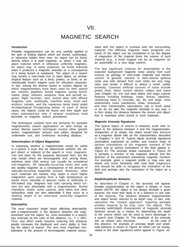
VII.
MAGNETIC SEARCH
Introduction
Portable magnetometers can be very usefully applied tothe task of finding objects which are buried, submerged,or otherwise hidden from view. An object can be founddirectly where it is itself magnetic, or where it may dis-place material which is otherwise uniformly magnetic.An object may, in some instances, be found indirectlywhen it produces a magnetic anomaly as a consequenceof it being buried or emplaced. The object of a searchmay involve a man-made iron or steel object, an archae-ological feature such as a brick, pottery, or tomb, or anintentionally buried magnet used for relocation purposes.In fact, among the diverse buried or sunken objects forwhich magnetometers have been used for their searchare: culverts, pipelines, buried magnets, survey bench-marks, ships, vehicles, weapons, boat and aircraft en-gines, flight recorder, skis, buried skier with affixedmagnets, rails, wellheads, machine tools, chain andanchors, tunnels, and the numerous items listed underArchaeological Prospecting below. In each of thesecases, the objects could be found and their depth andmass estimated-but only if several conditions existfavorable to magnetic search procedures.
The techniques outlined here are primarily for portablemagnetometer search applications on land except asnoted. Marine search techniques involve other specifictactics, magnetometer sensors and cables designed forunderwater use, and continuous recording displays.
Determination of Object Magnetism
In assessing whether a magnetometer would be usefulin a search, it must first be determined whether the ob-ject (direct or indirect) of the search is truly magnetic.Iron and steel, for the purposes discussed here, are theonly metals which are ferromagnetic and, among these,stainless steel (300 series) can usually be considerednon-magnetic. All naturally-occurring rocks and soilsare weakly magnetic as a consequence of the amount ofnaturally-occurring magnetite present. Moreover, whensuch materials are heated, they attain a much highermagnetism upon cooling from a high temperature aswould occur naturally in igneous rocks or artificially inkiln-baked clay. Magnets and coils carrying direct cur-rent are also detectable with a magnetometer. Buriedchambers, tombs, some caverns, lava tubes and othersubsurface voids are also detectable if they occur at ashallow depth in an otherwise uniformly magneticmaterial.
Detectability
The most important single factor affecting detectabilitywith a magnetometer is the distance between the mag-netometer and the object; for, most anomalies in a searchvary inversely as the cube of this distance, i.e., T = M/r3.Thus, any effort made towards reducing this distancegreatly increases the likelihood and one’s ability in find-ing the object of search. The next most important con-sideration is the amount of ferromagnetic material assoc-
39
iated with the object in contrast with the surroundingmaterial. The effective magnetic mass (magnetic mo-ment) of the object can be considered to be the degreeof magnetism of the material times the volume of suchmaterial (e.g., a small magnet can be as magnetic asan automobile or a very large cavern).
The last significant criterion for detectability is theexpected background magnetic noise arising from suchsources as geology or man-made materials and electriccurrent. In general, volcanic or dark-colored igneousrocks and soils derived from such rocks are very mag-netic and render it difficult to detect a small, subtleanomaly. Common artificial sources of noise includepower lines, direct current electric cables and trains(see Chapter IX), iron and steel debris and major culturalfeatures including buildings, roads, fences, pipelines,reinforcing steel in concrete, etc. By and large, mostsedimentary rocks (sandstone, shale, limestone, chert)and their metamorphic equivalents, salt or fresh wateror air do not alter the magnetic anomaly in any way; itis then simply the distance between the sensor and objectthat is important when buried in such materials.
Magnetic Anomaly Signatures
The typical object of search is relatively small with re-spect to the distance between it and the magnetometer.Irrespective of its shape, the object would then behaveas a magnetic dipole with all the characteristics describedin Chapters V and VI. Typical dipole anomaly signatures(anomalies) expressed as profiles and contour maps atvarious orientations of the magnetic moment of theobject and at various inclinations of the field appear inFigure 43. The anomaly shape expressed in Figure 43is primarily a function of the magnetic latitude and thedirection of the permanent (remanent) magnetic moment.For example, given a magnetic profile or map over anydipole and some familiarity with total field magneticsone should be able to recognize the inclination of thefield and perhaps also the orientation of the object as adipole.
Depth/Amplitude Behavior
As described in Chapter V, the anomaly will appearbroader proportionately as the object is deeper or moredistant (NOTE: the object is not always beneath a giventraverse, but more than likely is at a distance to one sideof the traverse. The distance between magnetometerand object herein referred to as depth may, in fact, onlyrepresent the ‘closest approach’ requiring perhapsanother traverse to be truly ‘over’ the object). Thisanomaly width/depth characteristic of magnetic anomalybehavior serves as a means for determining the depthto the source which can be used to one’s advantage ina search (see Chapter V). The amplitude of the anomalywill, as stated, also decrease inversely as the cube ofthis distance. An example of anomaly depth and ampli-tude behavior is shown in Figure 44 which can be extrap-olated to the other signatures which appear in Figure 43.
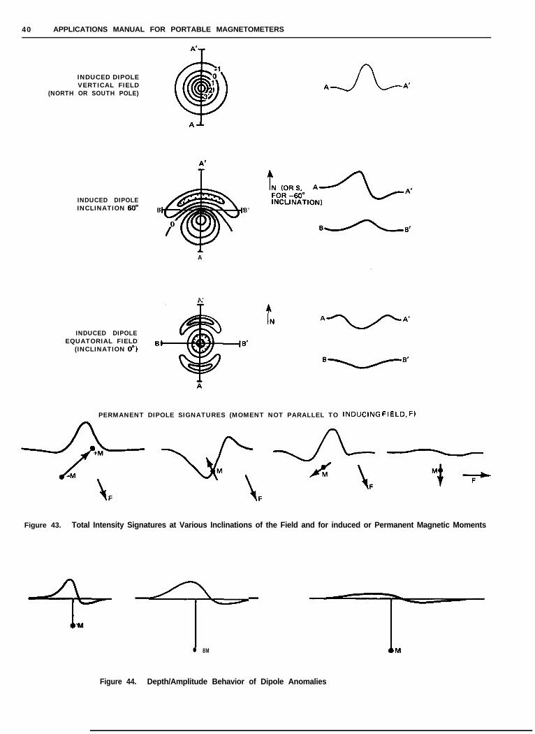
40 APPLICATIONS MANUAL FOR PORTABLE MAGNETOMETERS
INDUCED DIPOLEVERTICAL FIELD
(NORTH OR SOUTH POLE)
INDUCED DIPOLEINCLINATION 60”
INDUCED DIPOLEEQUATORIAL FIELD
(INCLINATION 0”)
B B’
A
A'
PERMANENT DIPOLE SIGNATURES (MOMENT NOT PARALLEL TO lNDUClNG FIELD, F)
Figure 43. Total Intensity Signatures at Various Inclinations of the Field and for induced or Permanent Magnetic Moments
4 --‘M
l 8M -I--Figure 44. Depth/Amplitude Behavior of Dipole Anomalies
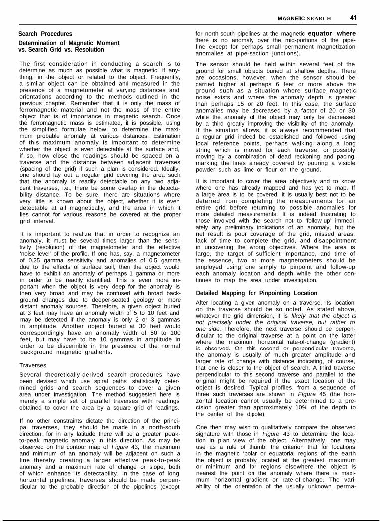
MAGNETIC SEARCH 41
Search ProceduresDetermination of Magnetic Momentvs. Search Grid vs. Resolution
The first consideration in conducting a search is todetermine as much as possible what is magnetic, if any-thing, in the object or related to the object. Frequently,a similar object can be obtained and measured in thepresence of a magnetometer at varying distances andorientations according to the methods outlined in theprevious chapter. Remember that it is only the mass offerromagnetic material and not the mass of the entireobject that is of importance in magnetic search. Oncethe ferromagnetic mass is estimated, it is possible, usingthe simplified formulae below, to determine the maxi-mum probable anomaly at various distances. Estimationof this maximum anomaly is important to determinewhether the object is even detectable at the surface and,if so, how close the readings should be spaced on atraverse and the distance between adjacent traverses(spacing of the grid) if such a plan is considered. Ideally,one should lay out a regular grid covering the area suchthat the anomaly is readily detectable on any two adja-cent traverses, i.e., there be some overlap in the detecta-bility distance. To be sure, there are situations wherevery little is known about the object, whether it is evendetectable at all magnetically, and the area in which itlies cannot for various reasons be covered at the propergrid interval.
It is important to realize that in order to recognize ananomaly, it must be several times larger than the sensi-tivity (resolution) of the magnetometer and the effective‘noise level’ of the profile. If one has, say, a magnetometerof 0.25 gamma sensitivity and anomalies of 0.5 gammadue to the effects of surface soil, then the object wouldhave to exhibit an anomaly of perhaps 1 gamma or morein order to be readily identified. This is even more im-portant when the object is very deep for the anomaly isthen very broad and may be confused with broad back-ground changes due to deeper-seated geology or moredistant anomaly sources. Therefore, a given object buriedat 3 feet may have an anomaly width of 5 to 10 feet andmay be detected if the anomaly is only 2 or 3 gammasin amplitude. Another object buried at 30 feet wouldcorrespondingly have an anomaly width of 50 to 100feet, but may have to be 10 gammas in amplitude inorder to be discernible in the presence of the normalbackground magnetic gradients.
Traverses
Several theoretically-derived search procedures havebeen devised which use spiral paths, statistically deter-mined grids and search sequences to cover a givenarea under investigation. The method suggested here ismerely a simple set of parallel traverses with readingsobtained to cover the area by a square grid of readings.
If no other constraints dictate the direction of the princi-pal traverses, they should be made in a north-southdirection, for in any latitude there will be a greater peak-to-peak magnetic anomaly in this direction. As may beobserved on the contour map of Figure 43, the maximumand minimum of an anomaly will be adjacent on such aline thereby creating a larger effective peak-to-peakanomaly and a maximum rate of change or slope, bothof which enhance its detectability. In the case of longhorizontal pipelines, traverses should be made perpen-dicular to the probable direction of the pipelines (except
for north-south pipelines at the magnetic equator wherethere is no anomaly over the mid-portions of the pipe-line except for perhaps small permanent magnetizationanomalies at pipe-section junctions).
The sensor should be held within several feet of theground for small objects buried at shallow depths. Thereare occasions, however, when the sensor should becarried higher at perhaps 6 feet or more above theground such as a situation where surface magneticnoise exists and where the anomaly depth is greaterthan perhaps 15 or 20 feet. In this case, the surfaceanomalies may be decreased by a factor of 20 or 30while the anomaly of the object may only be decreasedby a third greatly improving the visibility of the anomaly.If the situation allows, it is always recommended thata regular grid indeed be established and followed usinglocal reference points, perhaps walking along a longstring which is moved for each traverse, or possiblymoving by a combination of dead reckoning and pacing,marking the lines already covered by pouring a visiblepowder such as lime or flour on the ground.
It is important to cover the area objectively and to knowwhere one has already mapped and has yet to map. Ifa large area is to be covered, it is usually best not to bedeterred from completing the measurements for anentire grid before returning to possible anomalies formore detailed measurements. It is indeed frustrating tothose involved with the search not to ‘follow-up’ immedi-ately any preliminary indications of an anomaly, but thenet result is poor coverage of the grid, missed areas,lack of time to complete the grid, and disappointmentin uncovering the wrong objectives. Where the area islarge, the target of sufficient importance, and time ofthe essence, two or more magnetometers should beemployed using one simply to pinpoint and follow-upeach anomaly location and depth while the other con-tinues to map the area under investigation.
Detailed Mapping for Pinpointing LocationAfter locating a given anomaly on a traverse, its locationon the traverse should be so noted. As stated above,whatever the grid dimension, it is likely that the object isnot precisely under the original traverse, but rather toone side. Therefore, the next traverse should be perpen-dicular to the original traverse at a point on the latterwhere the maximum horizontal rate-of-change (gradient)is observed. On this second or perpendicular traverse,the anomaly is usually of much greater amplitude andlarger rate of change with distance indicating, of course,that one is closer to the object of search. A third traverseperpendicular to this second traverse and parallel to theoriginal might be required if the exact location of theobject is desired. Typical profiles, from a sequence ofthree such traverses are shown in Figure 45 (the hori-zontal location cannot usually be determined to a pre-cision greater than approximately 10% of the depth tothe center of the dipole).
One then may wish to qualitatively compare the observedsignature with those in Figure 43 to determine the loca-tion in plan view of the object. Alternatively, one mayuse as a rule of thumb, the criterion that for locationsin the magnetic ‘polar or equatorial regions of the earththe object is probably located at the greatest maximumor minimum and for regions elsewhere the object isnearest the point on the anomaly where there is maxi-mum horizontal gradient or rate-of-change. The vari-ability of the orientation of the usually unknown perma-
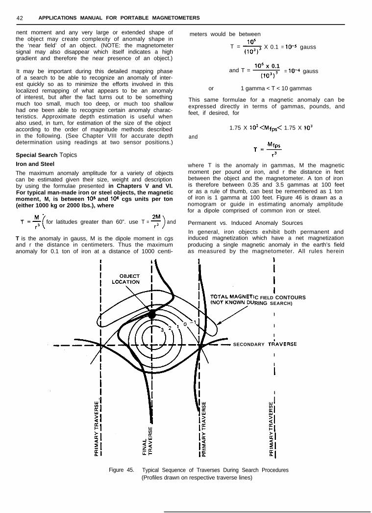
42 APPLICATIONS MANUAL FOR PORTABLE MAGNETOMETERS
nent moment and any very large or extended shape ofthe object may create complexity of anomaly shape inthe ‘near field’ of an object. (NOTE: the magnetometersignal may also disappear which itself indicates a highgradient and therefore the near presence of an object.)
It may be important during this detailed mapping phaseof a search to be able to recognize an anomaly of inter-est quickly so as to minimize the efforts involved in thislocalized remapping of what appears to be an anomalyof interest, but after the fact turns out to be somethingmuch too small, much too deep, or much too shallowhad one been able to recognize certain anomaly charac-teristics. Approximate depth estimation is useful whenalso used, in turn, for estimation of the size of the objectaccording to the order of magnitude methods describedin the following. (See Chapter VIII for accurate depthdetermination using readings at two sensor positions.)
Special Search TopicsIron and Steel
The maximum anomaly amplitude for a variety of objectscan be estimated given their size, weight and descriptionby using the formulae presented in Chapters V and VI.For typical man-made iron or steel objects, the magneticmoment, M, is between 105 and 106 cgs units per ton(either 1000 kg or 2000 Ibs.), where
for latitudes greater than 60”. use T = y>
and
T is the anomaly in gauss, M is the dipole moment in cgsand r the distance in centimeters. Thus the maximumanomaly for 0.1 ton of iron at a distance of 1000 centi-
meters would be between105
T =j X 0.1 = 10-S gauss(103)
and T =lo6 x 0.1
(1o3)3= 10-4 gauss
or 1 gamma < T < 10 gammas
This same formulae for a magnetic anomaly can beexpressed directly in terms of gammas, pounds, andfeet, if desired, for
and
1.75 X 10’ <Mfps< 1.75 X lo3
MfpsT=-r3
where T is the anomaly in gammas, M the magneticmoment per pound or iron, and r the distance in feetbetween the object and the magnetometer. A ton of ironis therefore between 0.35 and 3.5 gammas at 100 feetor as a rule of thumb, can best be remembered as 1 tonof iron is 1 gamma at 100 feet. Figure 46 is drawn as anomogram or guide in estimating anomaly amplitudefor a dipole comprised of common iron or steel.
Permanent vs. Induced Anomaly Sources
In general, iron objects exhibit both permanent andinduced magnetization which have a net magnetizationproducing a single magnetic anomaly in the earth’s fieldas measured by the magnetometer. All rules herein
C FIELD CONTOURSRING SEARCH)
I
I
I
SECONDARY TiAVERSE
I
I
I
I
I!I89
Figure 45. Typical Sequence of Traverses During Search Procedures(Profiles drawn on respective traverse lines)
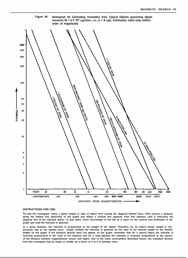
MAGNETIC SEARCH 43
400
300
200
100
1
50
40
8 30
2
d 20
10
5
4
3
2
1,
Figure 46. Nomogram for Estimating Anomalies from Typical Objects (assuming dipolemoment M = 5 X IO’ cgs/ton, i.e., k = 8 cgs. Estimates valid only withinorder of magnitude)
FEET 2 4 l b 20 80 100. . . $0 266
CENTIMETERS 100 200 400 600 6661066 20000 3600 4000
DISTANCE FROM MAGNETOMETER -
INSTRUCTIONS FOR USE:
To use the nomogram, select a given weight or type of object from among the diagonal labeled lines. Then choose a distancealong the bottom line (abscissa) of the graph and follow a vertical line upwards from that distance until it intersects thediagonal line of the selected object. At that point, move horizontally to the left to a value on the vertical axis (ordinate) of thegraph and read the intensity in gammas.
At a given distance, the intensity is proportional to the weight of the object. Therefore, for an object whose weight is notprecisely that of the labeled lines, simply multiply the intensity in gammas by the ratio of the desired weight to the labeledweight on the graph. If the distance desired does not appear on the graph, remember that for a typical object the intensity isinversely proportional to the cube of the distance and for a long pipeline the intensity is inversely proportional to the squareof the distance between magnetometer sensor and object. Due to the many uncertainties described herein, the estimates derivedfrom this nomogram may be larger or smaller by a factor of 2 to 5 or perhaps more.

44 APPLICATIONS MANUAL FOR PORTABLE MAGNETOMETERS
assume for simplicity, that the anomaly is produced bythe induced moment only. Nevertheless, the harder thesteel, the more permanent magnetization it possesses,which at times may be 10 times or more than the inducedmagnetization. Although one cannot usually predictthe orientation of the permanent moment of a buriedobject, it can be assumed that the larger the permanentmagnetization, the larger the anomaly and the suscepti-bility, k, used in the formulae herein is really an effec-tive k intended to include such increased magnetization.A single large part, such as a single pipe or an engine,etc., may exhibit one single anomaly due largely to thepermanent moment. Conversely, the more componentparts an object has, the more these individual permanentmagnetic moments tend to cancel, leaving only theinduced magnetization. When the permanent andinduced moments are of the same order of magnitude(see revolvers, for example, in table of anomalies on page46), and the permanent moment happens by chance tobe oriented in an opposite direction to the earth’s field,the observed anomaly would be very small, but almostnever zero. Whether or not an object has a large or smallpermanent moment is not consequential except in explain-ing the unusual shape of the anomalies one might observeas compared to the anomaly signatures shown in Figure43. (Note: Stainless steel, type 300, particularly Stainless310, is practically non-magnetic. Similarly, manganesesteel is only weakly magnetic.)
If one is able to measure the susceptibility, permeabilityor the magnetic moments by the procedures in ChapterVI, the following expression (also presented in ChapterVI) could be used to estimate the maximum anomalyamplitude
M = kFV
where M is the dipole magnetic moment in cgs units, kthe susceptibility which is between 1 and 10 cgs unitsfor most iron and steel objects, F the ambient field ingauss, and V the volume in cubic centimeters. If per-‘meability, I-(, is to be used, recall that ~1 = 1 + 4 1~ k,numerically. Attention should be paid to the effects ofdemagnetization (Chapter VI under “Systematic Rotationfor Magnitude and Direction”) which describes the factthat an anomaly from a more-or-less spherical iron objectmay not be as large as predicted from consideration ofI-( or k alone.
Pipelines (horizontal)
Most pipelines have very high permanent magnetizationand show separate anomalies for each length of pipe,i.e., anomalies at each joint due to their independentthermal and mechanical histories. Valves and otherattachments to pipelines show separate anomalies aswell. A horizontal pipeline in steeply dipping fields orE-W at the equator varies inversely as the square ofthe distance between its center and the magnetometerand behaves as a line of dipoles as described in ChapterV. Thus, the maximum anomaly amplitude from a pipe-line can be estimated as follows:
T,M,_=_kFA kF IT Dt
r2 r2 r2
where A is the approximate cross-sectional area of iron,and D and t are the pipe diameter and wall thicknessrespectively in the same dimensional units as the dis-tance, r, and the other factors as used above. For mostpipes, the steel is ‘hard’ and k (effective) is thereforehigh, perhaps, 10 to 50 cgs or higher. For example,
consider a horizontal pipeline diameter 6 inches, wallthickness l/4 inch in a field of 50,000 gammas buried ata depth of 20 feet beneath the magnetometer,
T =10X5X104X7rX6X$
(20X 12)2= 40gammas
The expression, fr Dt, represents the approximate crosssectional area of the thin wall of the pipe. A more pre-cise but more complicated expression for this areamight be (nROz -nRi’) where R, and Ri are the outside
and inside diameters of the pipe respectively.
For solid pipes, rods, or steel cable, a similar expressionis used,
kFA kF nR2T=-_=-r* r2
where R is the radius of the rod.
The anomaly signature for pipelines in various directionsand field inclinations would appear as in Figure47. (Notethe difficulties in detecting N-S pipelines in equatorialregions described above under “Traverses” and ChapterV.) The permanent magnetic moment is often predomi-nant in a pipeline and may commonly exhibit a signatureas shown in Figure 47 with the maxima and minimareversed and a very large amplitude. A pipeline is gen-erally easy to detect because its great length oftenassures one of actually crossing it. Also, the signaturevaries inversely as the square of the distance instead ofthe cube of the distance as in the case of a dipole (pipe-lines are lines of dipoles) and the anomaly amplitudethus remains large. If one has access to both ends of ahidden pipeline, it is also possible to pass a large DCcurrent through it to aid in its detection by enhancingits magnetic field selectively in space or time. For exam-ple, to find one pipeline out of many possible interferingpipelines, pass a current through it for one reading andreverse the current for the next, taking two such readingsat each point. The location of the one anomaly can beso mapped as the difference in these values becomeslarger as one is closer to the pipe. (1 ampere of currentthrough an infinitely long pipe would produce 10 gam-mas at 60 feet and would in this case produce 20 gam-mas peak-to-peak and vary inversely as the distance tothe pipe. However, observe the geometry noted inChapter IX.)
Magnetic Markers
It is often of interest to be able to relocate oneself oran object over a long period of time. The purpose maybe to locate a survey benchmark, an important junctionin a pipeline, or a point in shallow marine waters. Inlieu of a radio transmitter or other active source, it ispossible to bury a magnet which should keep most ofits magnetic moment for many years or longer and at adepth sufficiently below any level that is likely to bedisturbed. In some cases, it may be reasonable to buryseveral magnets oriented to produce maxima or minimaor in a pattern to assure easy relocation or to differentiateone magnetic marker from another. Given a specializedrequirement, a solenoid coil or single long wire withan applied direct current may also serve such a reloca-tion purpose.
A magnet of convenient size and made of Alnico V isavailable in the form of a thumb-size ‘cow-magnet’, a
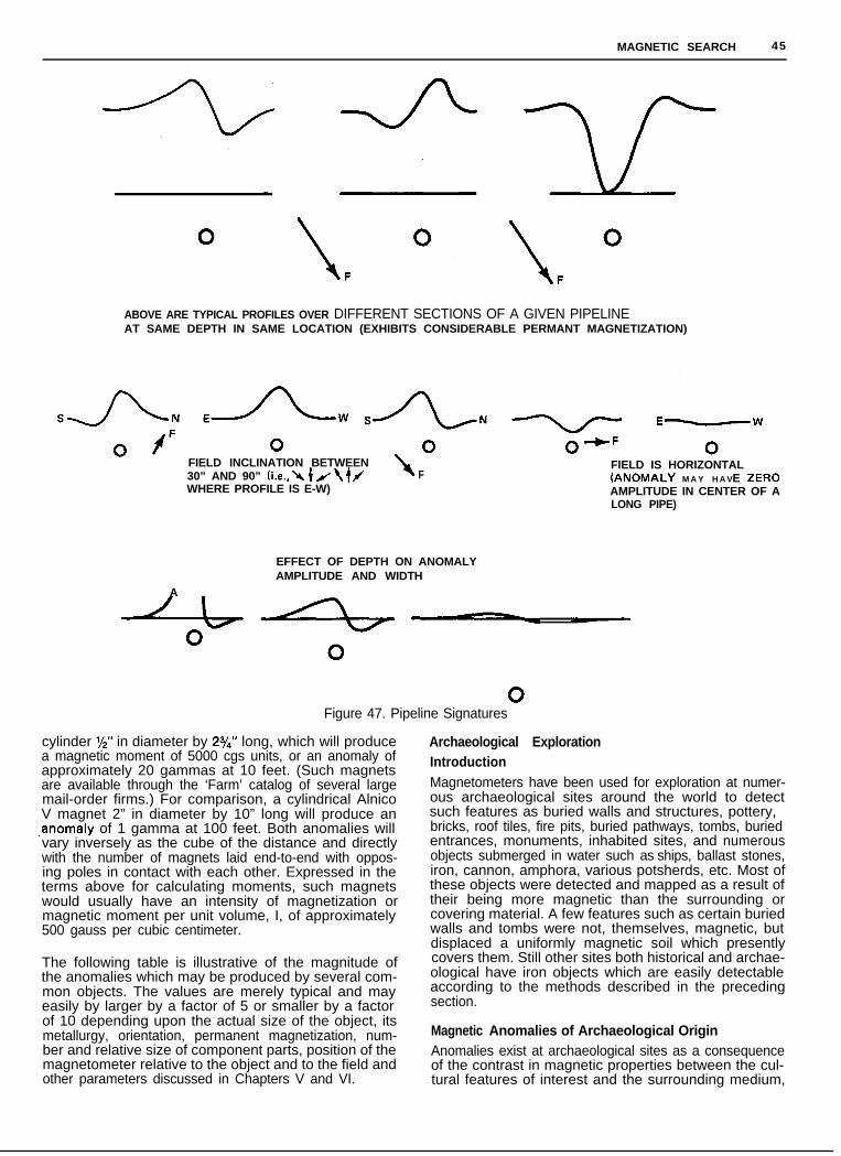
MAGNETIC SEARCH 45
ABOVE ARE TYPICAL PROFILES OVER DIFFERENT SECTIONS OF A GIVEN PIPELINEAT SAME DEPTH IN SAME LOCATION (EXHIBITS CONSIDERABLE PERMANT MAGNETIZATION)
0 0FIELD INCLINATION BETWEEN30” AND 90” (i.e.,\ 4 J f If FWHERE PROFILE IS E-W)
A
EFFECT OF DEPTH ON ANOMALYAMPLITUDE AND WIDTH
FIELD IS HORIZONTAL(ANOMALY M A Y H A VE 2~~0AMPLITUDE IN CENTER OF ALONG PIPE)
-Y--- -0
0Figure 47. Pipeline Signatures
cylinder 1/Z” in diameter by 23/4” long, which will producea magnetic moment of 5000 cgs units, or an anomaly ofapproximately 20 gammas at 10 feet. (Such magnetsare available through the ‘Farm’ catalog of several largemail-order firms.) For comparison, a cylindrical AlnicoV magnet 2” in diameter by 10” long will produce an,anomaly of 1 gamma at 100 feet. Both anomalies willvary inversely as the cube of the distance and directlywith the number of magnets laid end-to-end with oppos-ing poles in contact with each other. Expressed in theterms above for calculating moments, such magnetswould usually have an intensity of magnetization ormagnetic moment per unit volume, I, of approximately500 gauss per cubic centimeter.
The following table is illustrative of the magnitude ofthe anomalies which may be produced by several com-mon objects. The values are merely typical and mayeasily by larger by a factor of 5 or smaller by a factorof 10 depending upon the actual size of the object, itsmetallurgy, orientation, permanent magnetization, num-ber and relative size of component parts, position of themagnetometer relative to the object and to the field andother parameters discussed in Chapters V and VI.
Archaeological ExplorationIntroductionMagnetometers have been used for exploration at numer-ous archaeological sites around the world to detectsuch features as buried walls and structures, pottery,bricks, roof tiles, fire pits, buried pathways, tombs, buriedentrances, monuments, inhabited sites, and numerousobjects submerged in water such as ships, ballast stones,iron, cannon, amphora, various potsherds, etc. Most ofthese objects were detected and mapped as a result oftheir being more magnetic than the surrounding orcovering material. A few features such as certain buriedwalls and tombs were not, themselves, magnetic, butdisplaced a uniformly magnetic soil which presentlycovers them. Still other sites both historical and archae-ological have iron objects which are easily detectableaccording to the methods described in the precedingsection.
Magnetic Anomalies of Archaeological OriginAnomalies exist at archaeological sites as a consequenceof the contrast in magnetic properties between the cul-tural features of interest and the surrounding medium,
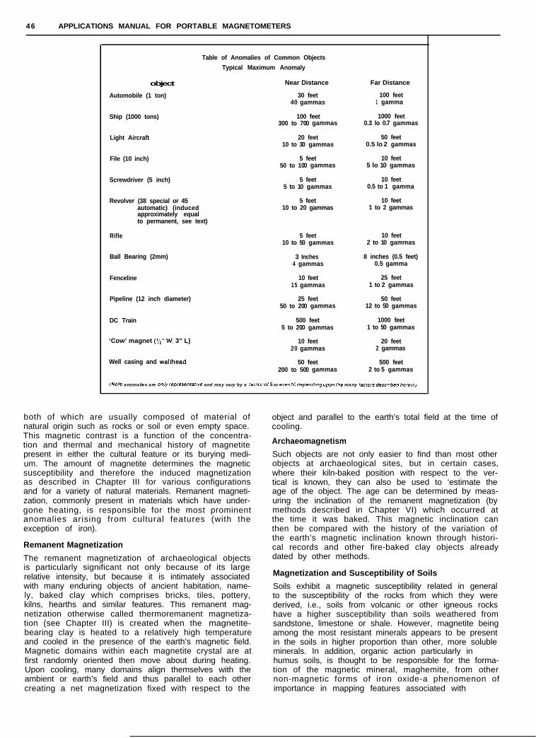
46 APPLICATIONS MANUAL FOR PORTABLE MAGNETOMETERS
Table of Anomalies of Common Objects
Typical Maximum Anomaly
object
Automobile (1 ton)
Ship (1000 tons)
Light Aircraft
File (10 inch)
Screwdriver (5 inch)
Revolver (38 special or 45automatic) (inducedapproximately equalto permanent, see text)
Near Distance Far Distance
30 feet 100 feet40 gammas 1 gamma
100 feet 1000 feet300 to 700 gammas 0.3 lo 0.7 gammas
20 feet 50 feet10 to 30 gammas 0.5 lo 2 gammas
5 feet 10 feet50 to 100 gammas 5 lo 10 gammas
5 feet 10 feet5 to 10 gammas 0.5 to 1 gamma
5 feet 10 feet10 to 20 gammas 1 to 2 gammas
Rifle 5 feet 10 feet10 to 50 gammas 2 to 10 gammas
Ball Bearing (2mm) 3 Inches 8 inches (0.5 feet)4 gammas 0.5 gamma
Fenceline 10 feet 25 feet15 gammas 1 to 2 gammas
Pipeline (12 inch diameter) 25 feet 50 feet50 to 200 gammas 12 to 50 gammas
DC Train 500 feet 1000 feet5 to 200 gammas 1 to 50 gammas
‘Cow’ magnet (%” W. 3” L) 10 feet 20 feet20 gammas 2 gammas
Well casing and wellhead 50 feet 500 feet200 to 500 gammas 2 to 5 gammas
(Note anomalies are on!y repre~enlalwe and may vary by a taclor 015 or even 10 dependmg upon the many tacror~ descrbed herern)
both of which are usually composed of material ofnatural origin such as rocks or soil or even empty space.This magnetic contrast is a function of the concentra-tion and thermal and mechanical history of magnetitepresent in either the cultural feature or its burying medi-um. The amount of magnetite determines the magneticsusceptibility and therefore the induced magnetizationas described in Chapter III for various configurationsand for a variety of natural materials. Remanent magneti-zation, commonly present in materials which have under-gone heating, is responsible for the most prominentanomalies arising from cultural features (with theexception of iron).
Remanent Magnetization
The remanent magnetization of archaeological objectsis particularly significant not only because of its largerelative intensity, but because it is intimately associatedwith many enduring objects of ancient habitation, name-ly, baked clay which comprises bricks, tiles, pottery,kilns, hearths and similar features. This remanent mag-netization otherwise called thermoremanent magnetiza-tion (see Chapter III) is created when the magnetite-bearing clay is heated to a relatively high temperatureand cooled in the presence of the earth’s magnetic field.Magnetic domains within each magnetite crystal are atfirst randomly oriented then move about during heating.Upon cooling, many domains align themselves with theambient or earth’s field and thus parallel to each othercreating a net magnetization fixed with respect to the
object and parallel to the earth’s total field at the time ofcooling.
Archaeomagnetism
Such objects are not only easier to find than most otherobjects at archaeological sites, but in certain cases,where their kiln-baked position with respect to the ver-tical is known, they can also be used to ‘estimate theage of the object. The age can be determined by meas-uring the inclination of the remanent magnetization (bymethods described in Chapter VI) which occurred atthe time it was baked. This magnetic inclination canthen be compared with the history of the variation ofthe earth’s magnetic inclination known through histori-cal records and other fire-baked clay objects alreadydated by other methods.
Magnetization and Susceptibility of Soils
Soils exhibit a magnetic susceptibility related in generalto the susceptibility of the rocks from which they werederived, i.e., soils from volcanic or other igneous rockshave a higher susceptibility than soils weathered fromsandstone, limestone or shale. However, magnetite beingamong the most resistant minerals appears to be presentin the soils in higher proportion than other, more solubleminerals. In addition, organic action particularly in high-humus soils, is thought to be responsible for the forma-tion of the magnetic mineral, maghemite, from othernon-magnetic forms of iron oxide-a phenomenon ofimportance in mapping features associated with habita-
MAGNETIC SEARCH 47
tion. Therefore, soils may have a somewhat highersusceptibility than would be indicated by the parentrock susceptibility, soils of 10-4 cgs being common. Thissurface magnetite is also a source of magnetic noisein precision magnetic surveys performed very close tothe surface of the ground when the magnetite, by theaction of surface waters and gravity, collects into smallpockets of placer magnetite common almost every-w h e r e in the microtopography of the ground surface.
Remanent Magnetization of Soils
Of additional significance to archaeological explorationis the presence in surface soils of remanent magnetiza-tion often with twice the intensity of induced magneti-zation. This magnetization is due sometimes to heating,but more probably to ‘viscous’ magnetization attainedslowly in place (during tens to thousands of years) andthe formation in situ of maghemite by the organic proc-esses cited above. This remanent magnetization is mostcommon in the upper layers of soil and if disturbed bycultivating, by digging graves, by foot or animal traffic,or by other physical disruption of the integrity of thesoil, is destroyed creating a locally negative anomaly,often mappable with a portable magnetometer.
Magnetic Anomaly Complexity
The anomalies observed at archaeological sites are inmost cases very complex as a consequence of severalfactors. The sources which produce the anomalies arerelatively shallow and therefore close to the magneto-meter which emphasizes the extremely complex natureof the ‘near field’ of any magnetic object. Also, the vari-ous sources of magnetic anomalies from soils, near sur-face rocks and the clutter of ancient or modern humanhabitation, including the very objects of interest, is oftenvery pronounced. The nature of the measurements oneobtains in archaeological exploration-closely spacedand near to the ground surface-makes the data seemmore noisy than they appear on the usual mineral explor-ation survey. An archaeological survey properly con-ducted, planned and interpreted, however, can oftenmake sense of this complexity and produce meaningfulinterpretations from individually resolvable, magneticarchaeological features.
Archaeological Survey Planning and Feasibility
Successful application of a magnetometer to archaeo-logical prospecting can assist an archaeological programin several ways. Most obviously, the specific site andfeatures which are hidden from view can be located,depths estimated and excavations conducted efficiently,rapidly and more economically than if the locationswere not known with any confidence. In some instances,excavations need not be performed at least initially,where boundaries of structures and the extent of thesite can be mapped through magnetic surveys, e.g.,salvage archaeology, extending known sites, etc.
Although it may be tempting to assume that a magneticsurvey may be useful in mapping and detecting featuresat a given site, it may be fair to state that most sites , apriori, are not amenable to this method . Features maynot present a detectable magnetic contrast, the mag-netic background noise may be excessive or the sitemay be better mapped through less sophisticated meanssuch as visually or other tried and true techniques.
The known features should first be considered or meas-ured by the techniques outlined in Chapter VI to deter-
mine if there is, in fact, a measureable magnetizationcontrast (estimated by methods of Chapter V). Repre-sentative samples of both the buried features as well asthe burying material should be measured with specialattention to such items as: fist-size samples of structures,fire-baked large objects, soil, soil intact (to preserveremanent magnetization), humus-rich material, culturalmaterial present in appreciable amounts, rocks whichare thought to underlie the site (which may create insur-mountable noise as from volcanic rocks or laterite) andother material which may be present in any significantway at the site.
Having measured the induced and remanent magnetiza-tion (not important to measure the directions), havingestimated the amplitude of the anomalies and havingdetermined the background magnetic noise, one maybe able to predict whether a magnetic survey would beof significance. One can never really be certain of itsfeasibility, to be sure, until a survey is attempted.
The depth and amplitude can then be used as criteriato determine the grid, or density of individual measure-ments. Commonly, the area is divided into manageablequadrangles perhaps one or two hundred feet on a sideand a rope, marked by colors, alternating at the gridpoints, is laid along one traverse line (or perhaps a ropegrid is constructed). Measurements are taken at eachpoint on the rope and the rope moved away one griddistance away from its first position, etc. Sometimescareful pacing between known grid points at the edgeof the quadrangle is sufficient for the measurements.A spring-wound reel fixed to the ground at one side ofthe quadrangle with a distance-marked cord attached tothe magnetometer-bearer is a very rapid means formeasuring distance. Care should be taken to make surea magnetic heading error does not occur when theoperator faces the other direction upon returning onalternating traverses. The measured or empirically-determined offset, however, can be applied to correctfor such an offset. Time variations may be removed, ifsmall or deep anomalies are sought, by methods inChapter IV using either a recording base station, tielines (two or more lines which cross the traverse lines),or re-occupied stations.
The data should then be contoured (see Chapter IV) andinterpreted in light of what is known about the site. Afterand during excavations, it may be useful to follow upthe survey by mapping select areas once again aftersome sources are removed and if the depth to featuresof interest is thus markedly decreased (by access todeep and wide holes and if the soil is not too magneticor magnetically disturbed).
Archaeological Anomaly Amplitude and Signatures
In order to estimate the maximum anomaly from anarchaeological object, consider the anomaly from asingle cube of rock representing perhaps a buriedmonument.
kF D3T=-r3
where T = the anomaly in gammas, k the susceptibilitycontrast per unit volume, F the earth’s field intensity ingammas, D the dimension of one side of the cube inthe same units as r, r the distance between the magneto-meter and center of the cube of rock in any distance
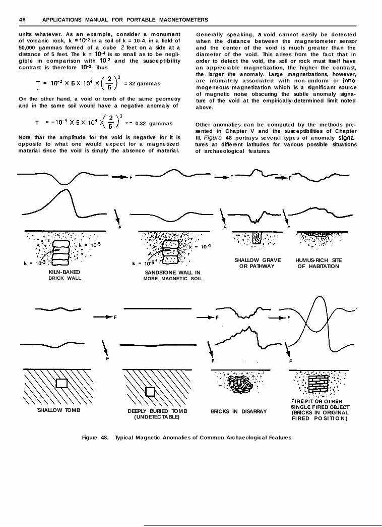
48 APPLICATIONS MANUAL FOR PORTABLE MAGNETOMETERS
units whatever. As an example, consider a monumentof volcanic rock, k = lo-2 in a soil of k = 10-4, in a field of50,000 gammas formed of a cube 2 feet on a side at adistance of 5 feet. The k = 1O-4 is so small as to be negli-gible in comparison with lo-2 and the susceptibilitycontrast is therefore 10-2. Thus
3= 32 gammas
On the other hand, a void or tomb of the same geometryand in the same soil would have a negative anomaly of
Generally speaking, a void cannot easily be detectedwhen the distance between the magnetometer sensorand the center of the void is much greater than thediameter of the void. This arises from the fact that inorder to detect the void, the soil or rock must itself havean appreciable magnetization, the higher the contrast,the larger the anomaly. Large magnetizations, however,are intimately associated with non-uniform or inho-mogeneous magnetization which is a significant sourceof magnetic noise obscuring the subtle anomaly signa-ture of the void at the empirically-determined limit notedabove.
T =-1O-4X5X1O4X f( >
3= - 0.32 gammas Other anomalies can be computed by the methods pre-
Note that the amplitude for the void is negative for it issented in Chapter V and the susceptibilities of Chapter
opposite to what one would expect for a magnetizedIll. Figure 48 portrays several types of anomaly signa-
material since the void is simply the absence of material.tures at different latitudes for various possible situationsof archaeological features.
SHALLOW GRAVE HUMUS-RICH SITEOR PATHWAY OF HABITATION
KILN-BAKED SANDSTONE WALL INBRICK WALL MORE MAGNETIC SOIL
SHALLOW TOMB DEEPLY BURIED TOMB BRICKS IN DISARRAY(UNDETECTABLE)
(BRICKS IN ORIGINALF I R E D P O S I T I O N )
Figure 48. Typical Magnetic Anomalies of Common Archaeological Features
VIII.
GRADIOMETERS AND GRADIENT TECHNIQUES
Introduction
It is of some interest in exploration to measure variousgradients, particularly the vertical gradient using a por-table magnetometer. The average horizontal gradientalong the traverse can easily be computed from theprofile, whereas the vertical gradient from typical, widely-spaced ground traverses cannot be accurately computed.A gradiometer is so named because it measures thegradient and in the context of the Manual, the gradientof the total field. In order to meet all the requirementsand applications suggested in this chapter, the gradiom-eter is here defined as a differential magnetometerwhere the spacing between sensors is fixed and smallwith respect to the distance to sources whose gradientsare to be measured. The difference in intensity dividedby the distance between sensors is then the gradientmeasured at the midpoint o f the sensor spacing. A quasi-differential magnetometer using a single instrumentwith successive measurements with the sensor at twoor more positions is suggested as more practical formost uses than a two sensor configuration.
Generally, it is more desirable for gradient measurementsto have higher sensitivity on the order perhaps of 0.25gammas for reasons that will become obvious, but 1gamma sensitivity is adequate when the anomalies andtheir gradients are relatively large. As an additional con-dition, it is relatively important in any ground gradientapplications that there be no significant surface mag-netic noise, for gradient anomalies tend to greatly en-hance such shallow noise sources which would bedetrimental for most objectives.
Applications of the Gradiometer
The vertical gradient or any gradient for that matter hasseveral properties of interest in exploration. First, gradi-ent anomalies tend to resolve composite or complexanomalies into their individual constituents and on thesame basis automatically remove the regional magneticgradient to better define the shallower anomaliesassumed to be of interest. Also, the magnetic time vari-ations including the effects of magnetic storms areeffectively removed. The measurements which comprisethe gradient are made almost simultaneously and veryclosely spaced compared to the source of magneticstorm effects and diurnal variations so that such effectson the two readings are essentially identical and there-fore removed on the differential. A third useful attributeof the gradients is that they can be used very quanti-tatively or for their vector properties (gradient of thescalar) in ascertaining anomaly depth, magnetic moment,shape. and location. These vector properties also allowuse of the vector diagram techniques formerly requiringthe more cumbersome horizontal and vertical componentmagnetometers or modified dip needles.
Use of a protable magnetometer as a gradiometer alsoinvolves several difficulties over use of the instrumentas a simple single-reading magnetometer. Some of the
applications require not just two but three or even fourseparate readings per station and the attendant additionaldata reduction efforts. The usual advantages of an orien-tation-insensitive scalar instrument represented by aproton magnetometer are partially defeated in the direc-tional requirements inherent in the two readings of agradiometer, albeit they are only on the order of f severaldegrees. Lastly, considerably more care must be takenin obtaining the data (e.g., magnetic cleanliness ofoperator, positioning of sensors, etc.) for a gradiometerimplies and utilizes higher resolution total intensitymeasurements. The proper application of the gradiom-eter techniques outlined in this Chapter, however, mayeasily justify such extra effort for many geological,search and other objectives.
Conditions for Gradient Measurement
As defined above, a gradiometer is first a differentialmagnetometer, i.e., a difference, AT, is measured orcomputed between two readings at different locations.For many if not most applications, the conventionaltotal field at one of the positions (in practice, eitherone) is also utilized. The word fixed is in the definitionto denote the difference between a gradiometer as usedhere, and a differential magnetometer where one sensoris fixed, the other traversing, connected so as to removetime variations.
The most significant requirement expressed in the defi-nition is that which requires that the spacing betweensensors, i.e., their positions of measurement, Ar, be smallwith respect to the distance, r, to the sources of theanomalies under investigation. If one considers a dipole,for example, one sensor at r would measure an anomalyT. A second sensor at 2 r would only measure y8 of T,i.e., the second sensor is essentially not sensing theanomaly at all and may as well be at infinity. The dif-ferential measurement in this case is, for all practicalpurposes, the same as the usual single sensor totalfield measurement. More specifically, the gradient canbe expressed as
AI lim Tr - Tr+Ar dT
Ar z Ar+O Ar =dr
where AT = T, - Tr+A,. is the total field differential between
two sensor positions spaced Ar apart and!!?is the deriva-dr
tive or gradient of T in the direction of r. The expression,Ar+o expresses the mathematical condition that Arshould be small with respect to r (in theory Ar should bezero). If Ar is less than 1/1,, r or even )!5 r, the conditionis well satisfied in the context of all suggested applica-tions. Usually there is no point in making Ar smallerthan 1/1,, r, for the gradiometer sensitivity (as expressedin the following) will be unjustifiably degraded. Practi-cal considerations as well limit both maximum andminimum Ar.
49
5 0 APPLICATIONS MANUAL FOR PORTABLE MAGNETOMETERS
(Note: as explained in Chapter II, a total field magnetom-eter measures only the vector component of any localanomaly in the undisturbed direction of the field. For alocal anomaly T, then, the magnetometer will measurethe component, TF, in the direction of F as previouslypresented. The gradiometer will then effectively measure
dTF
dr’i.e., the gradient in the direction r of the component
in the total field direction of the anomaly T.)
Gradiometer Sensitivity
The expressionAT dT.- ordrrs the measurement observedAr
with the gradiometer (after proper data reduction). Thegradiometer thus measures a gradient expressed ingammas per foot or gammas per meter, etc. in the direc-
dTtion of r (or the vertical gradienLZ, in the direction of
z) which may be contrasted with the basic magnetom-eter measurement of T (actually total field, F), whichis a scalar and inherently specifies no direction. (NOTE:the total field anomaly T is used herein instead of totalfield F to simplify and be more consistent in the expres-sions for the anomalies themselves).
The smaller the value of zthat the gradiometer can
measure, the more sensitive is the gradiometer. Thisvalue can, in turn, be made smaller by minimizing A Tor maximizing Ar. Thus, for a magnetometer with asensitivity of 1 gamma and spacing of 3 feet betweensensor positions, the gradient sensitivity would be‘/3 = 0.3 gamma per foot. For a magnetometer with0.25 gamma sensitivity and sensor spacing of 3 feet,
the gradient sensitivity is’*= 0.08 gamma per foot.3
Increasing the sensor spacing to 8 feet and using 0.25
gamma magnetometer sensitivity provides0.25- = 0.03
8gamma per foot sensitivity-adequate for many petro-leum exploration applications.
Gradiometer Readings in the Field
The gradiometer measurements incorporated- in some
dTof these applications are the vertical gradient - and
the two horizontal gradients, $ and dT, d.Zdy
z bemg the
vertical coordinate, x along the profile and y normal tothe profile. When these three gradients are used together,
the symbolism for partial derivatives, g , ?ay
and g
will be used, but they are the same numerically as theircorresponding expressions above.
A vertical differential reading can be obtained by usinga single magnetometer with the sensor placed first atone elevation and then another over the same point onthe traverse. Typical elevations are 4 feet and 8 feetfor very large gradients (mineral exploration or search)or 4 feet and 12 feet for smaller gradients, the largerthe separation the more sensitive the gradiometer. It isimportant in the vertical gradiometer observations thatthe sensor occupy the same horizontal position when
making each measurement. One possible arrangementis to place the sensor on a long staff and to place anadditional support or staff, at right angles to the princi-pal staff near the sensor. Thus, readings could then betaken on each of these staffs so long as adequate signalsare obtained for these orientations. (See Figure 49.)
Horizontal gradients can be computed from the totalfield data as the slope of the total field profile at anypoint of interest which is one example of the necessityfor total field, not simply vertical gradient alone. Ade-quate horizontal gradients can only be computed in thismanner when the anomalies are extremely broad, i.e.,the sources deep, relative to the station density, asmight be true for many petroleum surveys. In the case ofshallow anomaly sources as in mineral exploration wherethe total field variations and their gradients are largeand rapidly changing, the individual total field measure-ments may be spaced too far apart to allow for accurateslope measurements at the points where the verticalgradient is observed. In such surveys, the horizontalgradient can be measured in any of several ways withincreasing accuracy, but also increasing time and effort.
In theory, a gradiometer measures the gradient at themidpoint of the sensor spacing. Ideally therefore, onemay wish to measure the vertical gradient with twomeasurements above and below a point P and the hori-zontal gradient (or gradients) from two additional meas-urements in front and back of the same point for a totalof 4 measurements. A purist may also recommend thatwhere total field is required, it, too, should be measuredat P as a fifth measurement and if the other horizontalgradient is desired as well, it would involve 2 additionalobservations for a grand total of 7 readings.
In practice, however, particularly for sources deeperthan, say, 100 feet, what is recommended is simply threereadings, two spaced perhaps 8 feet apart at the higherelevation of 12 feet, and one beneath either of the firsttwo at an elevation of 4 feet. The assumption would bemade that all measurements were centered about thesame point (see Figure 49), as the ideal case above.
The lower reading of any vertical gradiometer pair ofmeasurements should seldom be made much closer thanseveral feet to the ground surface due to possible effectsof surface noise from the microtopography, placer mag-netite, etc. On the other hand, it is desirable to maxi-mize the separation between sensors to increase thesensitvitiy of the gradiometer without making the highersensor unwieldly and impractically high. The two sensorsin any configuration should not in general be off avertical or horizontal line by more than 5 or 10 degreesif at all possible, for one is making a vector (angular-dependent) measurement.
Gradiometer as a Filter
For reasons detailed in the following section below, thegradiometer automatically removes the regional gradient,and increases the resolution of even local anomalies(see Figure 50) . Each anomaly is portrayed as a moreresolved anomaly, separating, for example, the anomalyfrom different edges of a source into two or more dis-crete anomalies (see Figure 57) . This increased resolvingpower is exhibited by horizontal or vertical gradiometersequally well. The same property, however, precludesuseful application of a gradiometer in areas of surfacenoise, i.e., very local anomaly sources.
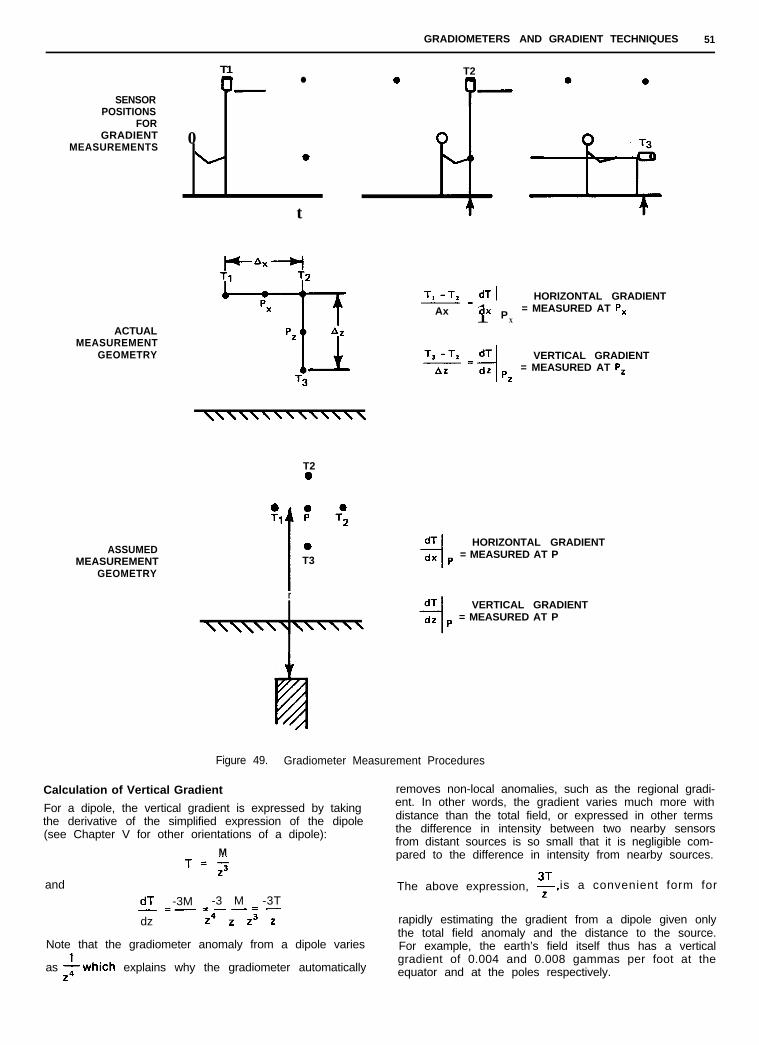
GRADIOMETERS AND GRADIENT TECHNIQUES 51
T1 T2l 0
SENSORPOSITIONS
FORGRADIENT
MEASUREMENTS0
0
t
ACTUALMEASUREMENT
GEOMETRY
ASSUMEDMEASUREMENT
GEOMETRY
T20
0 0 0TI P T2I 0
T3
r
T, -T, dT 1 HORIZONTAL GRADIENT- =Ax 1dx P
= MEASURED AT P,X
VERTICAL GRADIENT-== MEASURED AT P,
z
HORIZONTAL GRADIENT= MEASURED AT P
VERTICAL GRADIENT= MEASURED AT P
Figure 49. Gradiometer Measurement Procedures
Calculation of Vertical Gradient
For a dipole, the vertical gradient is expressed by takingthe derivative of the simplified expression of the dipole(see Chapter V for other orientations of a dipole):
M
T=;5and
dT -3M -3 M -3T_=_=--=-dz Z4 z z3 z
Note that the gradiometer anomaly from a dipole varies
as Iwhich explains why the gradiometer automaticallyz4
removes non-local anomalies, such as the regional gradi-ent. In other words, the gradient varies much more withdistance than the total field, or expressed in other termsthe difference in intensity between two nearby sensorsfrom distant sources is so small that it is negligible com-pared to the difference in intensity from nearby sources.
3T is a convenient form forThe above expression, ?,
rapidly estimating the gradient from a dipole given onlythe total field anomaly and the distance to the source.For example, the earth’s field itself thus has a verticalgradient of 0.004 and 0.008 gammas per foot at theequator and at the poles respectively.
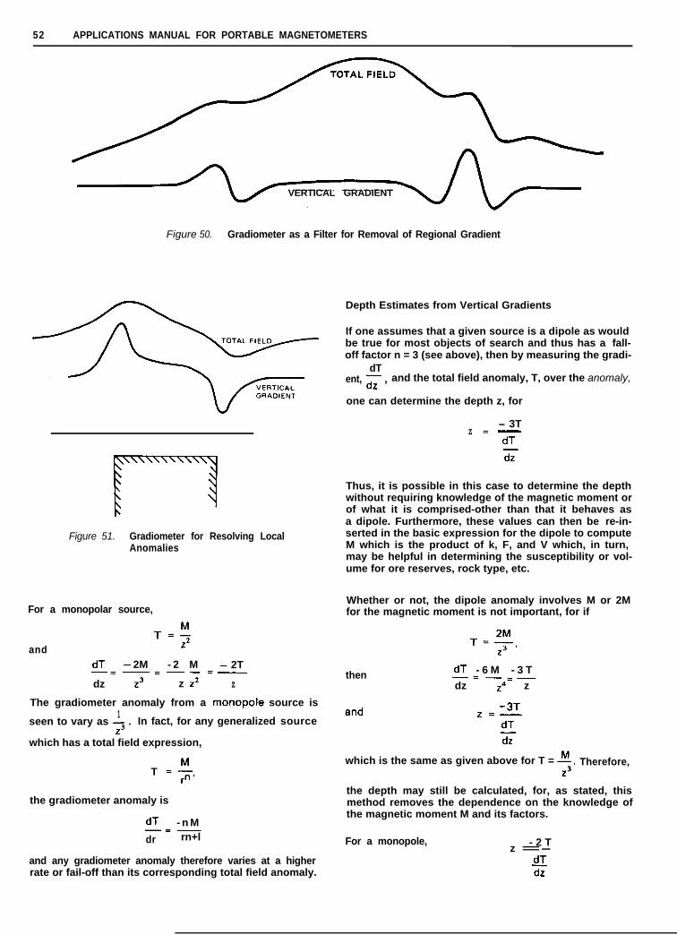
52 APPLICATIONS MANUAL FOR PORTABLE MAGNETOMETERS
VERTICAL GRADIENT
Figure 50. Gradiometer as a Filter for Removal of Regional Gradient
mFigure 51. Gradiometer for Resolving Local
Anomalies
For a monopolar source,
T=M
and z2
dT - 2M - 2 M - 2T-=-=--=_dz z3 z z2 Z
The gradiometer anomaly from a monopole source is1
seen to vary as - .Z3
In fact, for any generalized source
which has a total field expression,
T =$,
the gradiometer anomaly is
dT - n M-=-dr rn+l
and any gradiometer anomaly therefore varies at a higherrate or fail-off than its corresponding total field anomaly.
Depth Estimates from Vertical Gradients
If one assumes that a given source is a dipole as wouldbe true for most objects of search and thus has a fall-off factor n = 3 (see above), then by measuring the gradi-
dTent, ;;;- , and the total field anomaly, T, over the anomaly,
one can determine the depth z, for
- 3TZ=dT
z
Thus, it is possible in this case to determine the depthwithout requiring knowledge of the magnetic moment orof what it is comprised-other than that it behaves asa dipole. Furthermore, these values can then be re-in-serted in the basic expression for the dipole to computeM which is the product of k, F, and V which, in turn,may be helpful in determining the susceptibility or vol-ume for ore reserves, rock type, etc.
Whether or not, the dipole anomaly involves M or 2Mfor the magnetic moment is not important, for if
T=Mz3 ’
then dT - 6 M - 3 T-=-=_dz z*l z
z =-3TdTZ
which is the same as given above for T = 4.Z3
Therefore,
the depth may still be calculated, for, as stated, thismethod removes the dependence on the knowledge ofthe magnetic moment M and its factors.
For a monopole, - 2 Tz =-dTdz
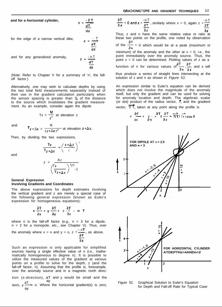
GRADIOMETERS AND GRADIENT TECHNIQUES 53
and for a horizontal cylinder, - 2 Tz=-
dTZ-
for the edge of a narrow vertical dike, - Tz=-dT
dz
and for any generalized anomaly, - n Tz=-dT
dz
aT - n Tx=Oandz=E,
- n Tsimilarly where x = 0, again z =-
aTZ Z
Thus, z and n have the same relative value or ratio atthese two points on the profile, one noted by observation
aTof the - =
ax0 which would be at a peak (maximum or
minimum) of the anomaly and the other at x = 0, i.e., thepoint immediately over the anomaly source. Thus, thepoint x = 0 can be determined. Plotting values of z as a
aT aT
(Note: Refer to Chapter V for a summary of ‘n’, the fall-off factor.)
function of n for various values of ax , az and x will
thus produce a series of straight lines intersecting at thesolution of z and n as shown in Figure 52.
Alternatively, one may wish to calculate depths by using An expression similar to Euler’s equation can be derivedthe two total field measurements separately instead of which does not involve the magnitude of the anomalytheir use in the gradient calculation particularly when itself, but only the gradient and can be used for solvingthe sensor spacing is greater than ‘15 of the distance for anomaly location and depth. The algebraic scalarto the source which invalidates the gradient measure- (or dot) product of the radius vector, ?, and the gradientment. As an example, consider again the dipole vector, VT, taken at any point along the profile is
Tz = $ at elevation z a-r aT aT - ax -+ y -
ax av+ z-g= IVTl Irlcost9
and MT*+Az =
(z+Az )3at elevation z+Az.
Then, by dividing the two expressions,
TZ z+Az-=-Tz +Az ( )
3 FOR DIPOLE AT z = 2.5ANDn=3
andZ
AZz =
Tz
( )
l/3
-1Tz+Az
General ExpressionInvolving Gradients and Coordinates
The above expressions for depth estimates involvingthe vertical gradient and z are merely a special case ofthe following general expression (known as Euler’sexpression for homogeneous equations):
t
2
z1
/
aT aT aTx -+ y-+ z - = - n T
ax ay az
where n is the fall-off factor (e.g., n = 3 for a dipole,n = 2 for a monopole, etc., see Chapter V). Thus, over
the anomaly where x = o and y = o, z =-z, as above.aT
az
Such an expression is only applicable for simplifiedsources having a single effective value of n (i.e., mathe-matically homogeneous to degree n). It is possible toutilize the measured values of the gradient at variouspoints on a profile to solve for the depth, z (and thefall-off factor, n). Assuming that the profile is, forexample,over the anomaly source and in a magnetic north direc-
FOR HORIZONTAL CYLINDERATDEPTHz=4ANDn=2
n
tion (x-direction), aT and y would be small and the
aT ayterm, y --x o. Where the horizontal gradient(s) is zero,
ay
Figure 52. Graphical Solution to Euler’s Equationfor Depth and Fall-off Rate for Typical Case
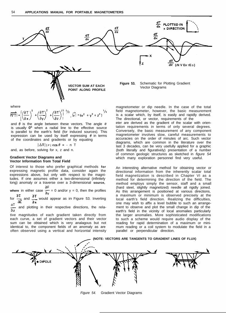
54 APPLICATIONS MANUAL FOR PORTABLE MAGNETOMETERS
VECTOR SUM AT EACHPOINT ALONG PROFILE
where
lE?=[(~,’ +(E.J +(zg %, <I = lx2 +y2+z?2and 8 is the angle between these vectors. The angle f?is usually 0” when a radial line to the effective sourceis parallel to the earth’s field (for induced sources). Thisexpression can be used by itself expressing 6’ in termsof the coordinates and gradients or by equating
IATl Irlcos0 = - n Tand, as before, solving for x, z and n.
Gradient Vector Diagrams andVector Information from Total Field
Of interest to those who prefer graphical methods forexpressing magnetic profile data, consider again theexpressions above, but only with respect to the magni-tudes. If one assumes either a two-dimensional (infinitelylong) anomaly or a traverse over a 3-dimensional source,
where in either case g = 0 and/or y = 0, then the profiles
for !?_ and g would appear as in Figure 53. Inverting
aTaZ
Zand plotting in their respective directions, the rela-
tive magnitudes of each gradient taken directly fromeach curve, a set of gradient vectors and their vectorsum can be obtained which is very analagous but notidentical to, the component fields of an anomaly as areoften observed using a vertical and horizontal intensity
dTudz (IN V ER TE D )
Figure 53. Schematic for Plotting GradientVector Diagrams
magnetometer or dip needle. In the case of the totalfield magnetometer, however, the basic measurementis a scalar which, by itself, is easily and rapidly derived.The directional, or vector, requirements of the gradiom-eter are derived as the gradient of the scalar with orien-tation requirements in terms of only several degrees.Conversely, the basic measurement of any componentmagnetometer involves slow, careful measurements toaccuracies on the order of minutes of arc. Such vectordiagrams, which are common in the literature over thelast 3 decades, can be very usefully applied for a graphic(both literally and figuratively) presentation of a numberof common geologic structures as sketched in figure 54which many exploration personnel find very useful.
An interesting alternative method for obtaining vector ordirectional information from the inherently scalar totalfield magnetization is described in Chapter VI as amethod for determining the direction of the field. Themethod employs simply the sensor, staff and a small(hard steel, slightly magnetized) needle all rigidly joined.As this arrangement is positioned at various directions,a maximum or minimum is observed precisely at thelocal earth’s field direction. Realizing the difficulties,one may wish to affix a level bubble to such an arrange-ment to observe and plot the small change in dip of theearth’s field in the vicinity of local anomalies particularlythe larger anomalies. More sophisticated modificationsto such a scheme would require audio display of thereading for rapid determination of a maximum or mini-mum reading or a coil system to modulate the field in aparallel or perpendicular direction.
(NOTE: VECTORS ARE TANGENTS TO GRADIENT LINES OF FLUX)
Figure 54. Gradient Vector Diagrams
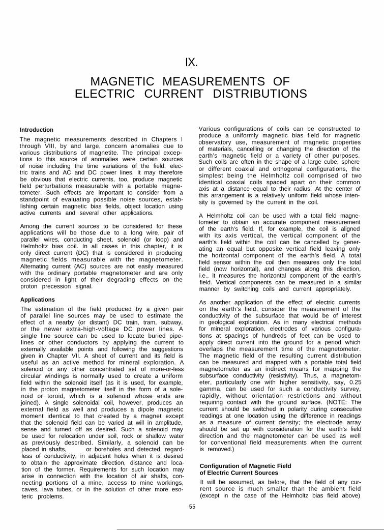
IX.
MAGNETIC MEASUREMENTS OFELECTRIC CURRENT DISTRIBUTIONS
Introduction
The magnetic measurements described in Chapters Ithrough VIII, by and large, concern anomalies due tovarious distributions of magnetite. The principal excep-tions to this source of anomalies were certain sourcesof noise including the time variations of the field, elec-tric trains and AC and DC power lines. It may thereforebe obvious that electric currents, too, produce magneticfield perturbations measurable with a portable magne-tometer. Such effects are important to consider from astandpoint of evaluating possible noise sources, estab-lishing certain magnetic bias fields, object location usingactive currents and several other applications.
Among the current sources to be considered for theseapplications will be those due to a long wire, pair ofparallel wires, conducting sheet, solenoid (or loop) andHelmholtz bias coil. In all cases in this chapter, it isonly direct current (DC) that is considered in producingmagnetic fields measurable with the magnetometer.Alternating current (AC) sources are not easily measuredwith the ordinary portable magnetometer and are onlyconsidered in light of their degrading effects on theproton precession signal.
Applications
The estimation of the field produced by a given pairof parallel line sources may be used to estimate theeffect of a nearby (or distant) DC train, tram, subway,or the newer extra-high-voltage DC power lines. Asingle line source can be used to locate buried pipe-lines or other conductors by applying the current toexternally available points and following the suggestionsgiven in Chapter VII. A sheet of current and its field isuseful as an active method for mineral exploration. Asolenoid or any other concentrated set of more-or-lesscircular windings is normally used to create a uniformfield within the solenoid itself (as it is used, for example,in the proton magnetometer itself in the form of a sole-noid or toroid, which is a solenoid whose ends arejoined). A single solenoidal coil, however, produces anexternal field as well and produces a dipole magneticmoment identical to that created by a magnet exceptthat the solenoid field can be varied at will in amplitude,sense and turned off as desired. Such a solenoid maybe used for relocation under soil, rock or shallow wateras previously described. Similarly, a solenoid can beplaced in shafts, adits or boreholes and detected, regard-less of conductivity, in adjacent holes when it is desiredto obtain the approximate direction, distance and loca-tion of the former. Requirements for such location mayarise in connection with the location of air shafts, con-necting portions of a mine, access to mine workings,caves, lava tubes, or in the solution of other more eso-teric problems.
Various configurations of coils can be constructed toproduce a uniformly magnetic bias field for magneticobservatory use, measurement of magnetic propertiesof materials, cancelling or changing the direction of theearth’s magnetic field or a variety of other purposes.Such coils are often in the shape of a large cube, sphereor different coaxial and orthogonal configurations, thesimplest being the Helmholtz coil comprised of twoidentical coaxial coils spaced apart on their commonaxis at a distance equal to their radius. At the center ofthis arrangement is a relatively uniform field whose inten-sity is governed by the current in the coil.
A Helmholtz coil can be used with a total field magne-tometer to obtain an accurate component measurementof the earth’s field. If, for example, the coil is alignedwith its axis vertical, the vertical component of theearth’s field within the coil can be cancelled by gener-ating an equal but opposite vertical field leaving onlythe horizontal component of the earth’s field. A totalfield sensor within the coil then measures only the totalfield (now horizontal), and changes along this direction,i.e., it measures the horizontal component of the earth’sfield. Vertical components can be measured in a similarmanner by switching coils and current appropriately.
As another application of the effect of electric currentson the earth’s field, consider the measurement of theconductivity of the subsurface that would be of interestin geological exploration. As in many electrical methodsfor mineral exploration, electrodes of various configura-tions at spacings of hundreds of feet can be used toapply direct current into the ground for a period whichoverlaps the measurement time of the magnetometer.The magnetic field of the resulting current distributioncan be measured and mapped with a portable total fieldmagnetometer as an indirect means for mapping thesubsurface conductivity (resistivity). Thus, a magnetom-eter, particularly one with higher sensitivity, say, 0.25gamma, can be used for such a conductivity survey,rapidly, without orientation restrictions and withoutrequiring contact with the ground surface. (NOTE: Thecurrent should be switched in polarity during consecutivereadings at one location using the difference in readingsas a measure of current density; the electrode arrayshould be set up with consideration for the earth’s fielddirection and the magnetometer can be used as wellfor conventional field measurements when the currentis removed.)
Configuration of Magnetic Fieldof Electric Current Sources
It will be assumed, as before, that the field of any cur-rent source is much smaller than the ambient field(except in the case of the Helmholtz bias field above)
55
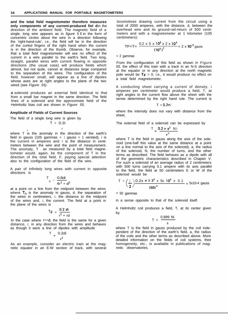
56 APPLICATIONS MANUAL FOR PORTABLE MAGNETOMETERS
and the total field magnetometer therefore measuresonly components of any current-produced fiel d in thedirection of the ambient field. The magnetic field of asingle, long wire appears as in figure 5 5 in the form ofconcentric circles about the wire in a direction followingthe ‘right-hand-rule’, i.e., the field will be in the directionof the curled fingers of the right hand when the currentis in the direction of the thumb. Observe, for example,that a total field magnetometer will see no effect of thecurrent in a wire parallel to the earth’s field. Two long,straight, parallel wires with current flowing in oppositedirections (the usual case) will produce fields whichalmost, but not quite, cancel at distances large comparedto the separation of the wires. The configuration of thefield, however small, will appear as a line of dipoleswhose axes are at right angles to the plane of the twowired (see Figure 55).
A solenoid produces an external field identical to thatfrom a small bar magnet in the same direction. The fieldlines of a solenoid and the approximate field of theHelmholtz bias coil are shown in Figure 55.
Amplitude of Fields of Current Sources
The field of a single long wire is given byT = 0.2i
. rwhere T is the anomaly in the direction of the earth’sfield in gauss (105 gammas = 1 gauss = 1 oersted), i isthe current in amperes and r is the distance in centi-meters between the wire and the point of measurement.The anomaly, T , as measured by a total field magne-tometer would, again, be the component of T in thedirection of the total field, F, paying special attentionalso to the configuration of the field of the wire.
A pair of infinitely long wires with current in oppositedirections is
Tn
= 0.8di
4rZ + d2at a point on a line from the midpoint between the wireswhere T, is the anomaly in gauss, d, the separation ofthe wires in centimeters, r, the distance to the midpointof the wires and, i, the current. The field at a point inthe plane of the wires is
Te = o’2 dir2 + rd
In the case where r>>d, the field is the same for a givendistance, r, in any direction from the wires and behavesas though it were a line of dipoles with amplitude
T = 0.2di
r2As an example, consider an electric train at the mag-netic equator in an E-W section of track, with several
locomotives drawing current from the circuit using atotal of 2000 amperes, with the distance, d, between theoverhead wire and its ground-rail-return of 500 centi-meters and with a magnetometer at 1 kilometer (105centimeters):
TF=T=0.2 x 5 x lo2 x 2 x lo3
(10s)2= 2 x 1o-5 gauss
= 2 gammas
From the configuration of this field as shown in Figure55, the effect of this train with a track in an N-S directionat the equator or in any direction at the north magneticpole would be TF = 0, i.e., it would produce no effect ona total field magnetometer.
A conducting sheet carrying a current of density, iamperes per centimeter would produce a field, T, atright angles to the current flow above the sheet with thesense determined by the right hand rule. The current is
T = 0.2ni
where the intensity does not vary with distance from thesheet.
The external field of a solenoid can be expressed by
T = 0.277 a2 N i
r3where T is the field in gauss along the axis of the sole-noid (one-half this value at the same distance at a pointon a line normal to the axis of the solenoid), a, the radiusof the solenoid, N, the number of turns, and the otherterms as described. The field behaves as a dipole with allof the geometric characteristics described in Chapter V.For such a solenoid of an average radius of 2 centimeterswith 500 turns carrying 0.1 ampere with its axis parallelto the field, the field at 50 centimeters E or W of thesolenoid would be
T = 1( >
0.2x 77X 22 x 5x lo2 x 0.1
1= 5x10⁻⁴ gauss
(50)3
= 50 gammas
in a sense opposite to that of the solenoid itself.
A Helmholtz coil produces a field, T, at its center givenby
0.899 NiT =
awhere T is the field in gauss produced by the coil inde-pendent of the direction of the earth’s field, a, the radiusof the coils and the other terms as described above. Moredetailed information on the fields of coil systems, theirhomogeneity, etc., is available in publications of mag-netic observatories.

MAGNETIC MEASUREMENTS OF ELECTRIC CURRENT DlSTRlBUTlONS 57
LONG STRAIGHT WIRE
c u r r e n t 3OUT OF
‘AGE
T FT
Yt
SOLENOID
CURRENT SHEET
PARALLEL WIRES:
Figure 55. Configuration of Magnetic Field of Various Electric Current Sources
58 APPLICATIONS MANUAL FOR PORTABLE MAGNETOMETERS
REFERENCES
Aitken, M.J., Physics and Archaeology : Interscience, London, 1961.
Archaeometry , a quarterly journal of The Research Laboratory for Archaeology andthe History of Art, Oxford University: Cambridge University Press, London.
Bossolasco, M., Editor, Pure and Applied Geophysics , a quarterly journal: Birkhauser Verlag, Basel.
Bozorth, R. Ferromagnetism : Van Nostrand, New York, 1951.
Chapman, S., and Bartels, J., Geomagnetism , Vol. I and II: Oxford University Press, London, 1940.
Dobrin, M.B., introduction to Geophysical Prospectihg : McGraw-Hill, New York, 1960.
Geoexploration , a quarterly journal: Elsevier, Amsterdam.
Geomagnetism and Geoelectricity , a monthly journal: University of Tokyo.
Geophysical Case Histories , Vol. I and II: Society of Exploration Geophysicists,Tulsa, 1948, 1956.
Geophysical Prospecting , a quarterly journal: European Association of ExplorationGeophysicists, The Hague.
Geophysics , a bi-monthly journal: Society of Exploration Geophysicists, Tulsa.
Grant, F.S. and West, G.F., Interpretation Theory in Applied Geophysics : McGraw-Hill, New York, 1965.
Haalck, H., Lehrbuch der Angewandten Geophysik : Berlin, 1934.
Heiland, C.A., Geophysical Exploration, afner, New York, 1940.
Izvestia, Series Geophysics , a monthly journal: Academy of Sciences of the USSR,Moscow.
Jakosky, J.J., Exploration Geophysics : Trija, Los Angeles, 1957.
Mining Geophysics , Vol. I and II: Society of Exploration Geophysicists, Tulsa, 1967.
Landsberg, H.E., editor, Advances in Geophysics , Vol. 1-15: Academic Press, New York.
Morley, L.W., editor, Mining and Ground Water Geophysics , Economic Geology Report No. 26: Depart-ment of Energy, Mines and Resources, Ottawa, 1970.
Nagata, T., Rock Magnetism : Maruzen, Tokyo, 1961.
Nettleton, L.L., Geophysical Prospecting for Oil : McGraw-Hill, New York, 1940.
Parasnis, D.S., Principles of Applied Geophysics : John Wiley and Sons, New York, 1962.
Prospezioni Archaeologiche , an annual journal: Lerici Fondazioni, Rome.
Runcorn, S.K., editor, Methods and Techniques in Geophysics : Interscience, N.Y., 1960.
Transactions, American institute of Mining and Metallurgical Engineers , Geophysics,a journal: AIME, New York.
www.alphageofisica.com.br