application of convolution theorems in semiparametric models with non-i.i.d. data
TRANSCRIPT
Journal of Statistical Planning andInference 91 (2000) 441–480
www.elsevier.com/locate/jspi
Application of convolution theorems in semiparametricmodels with non-i.i.d. data
Brad McNeneya;b;c;∗; 1, Jon A. Wellnerc;2aStatistics, North Carolina State University, Campus Box 8203, Raleigh, NC 27695-8203, USA
bNational Institute of Statistical Sciences, 19 TW Alexander Dr., P.O. Box 14006,Research Triangle Park, NC 27709-4006, USA
cUniversity of Washington, Statistics, Box 354322, Seattle, WA 98195-4322, USA
Abstract
A useful approach to asymptotic e�ciency for estimators in semiparametric models is thestudy of lower bounds on asymptotic variances via convolution theorems. Such theorems areoften applicable in models in which the classical assumptions of independence and identicaldistributions fail to hold, but to date, much of the research has focused on semiparametric modelswith independent and identically distributed (i.i.d.) data because tools are available in the i.i.d.setting for verifying pre-conditions of the convolution theorems. We develop tools for non-i.i.d.data that are similar in spirit to those for i.i.d. data and also analogous to the approaches usedin parametric models with dependent data. This involves extending the notion of the tangentvector �guring so prominently in the i.i.d. theory and providing conditions for smoothness, ordi�erentiability, of the parameter of interest as a function of the underlying probability measures.As a corollary to the di�erentiability result we obtain su�cient conditions for equivalence, interms of asymptotic variance bounds, of two models. Regularity and asymptotic linearity ofestimators are also discussed. c© 2000 Elsevier Science B.V. All rights reserved.
MSC: primary 60F05; 60F17; secondary 60J65; 60J70
Keywords: Convolution theorem; Asymptotic e�ciency; Information bound; Semiparametricmodel; Local asymptotic normality; Di�erentiability; Regular estimator
1. Introduction
Given a number of choices for making inference from observed data or, more par-ticularly, estimating parameters, an important goal is to identify the procedure that
∗ Correspondence address: University of Washington, Statistics, Box 354322, Seattle, WA 98195-4322,USA.E-mail addresses: [email protected] (B. McNeney), [email protected] (J.A. Wellner).1 Supported in part by NIH grants DK-42654 and R01 CA-5196 and R01 CA-519622.2 Supported in part by National Science Foundation grant DMS-9532039 and NIAID grant 2R01
AI291968-04.
0378-3758/00/$ - see front matter c© 2000 Elsevier Science B.V. All rights reserved.PII: S0378 -3758(00)00193 -2
442 B. McNeney, J.A. Wellner / Journal of Statistical Planning and Inference 91 (2000) 441–480
makes the best use of available data. Unfortunately, even conceptually simple exper-iments often lead to statistical models in which it is extremely di�cult to describeperformance of estimators in �nite samples. The simpli�cation in the structure of themodel obtained when the sample size tends to in�nity is often the only way to obtaina tractable notion of optimality. The hope is that estimators determined to be optimalin an asymptotic sense may be expected to perform well in the �nite samples obtainedin practice.A relatively well-studied concept of e�ciency is based on what are commonly re-
ferred to as convolution theorems. The two key hypotheses of such a theorem are localasymptotic normality (LAN) and di�erentiability of the parameter of interest. The latterrequires that this parameter, which could take values in an in�nite-dimensional space,represents a smooth function of the probability measures in the underlying statisticalmodel. Under these hypotheses, convolution theorems assert a minimum asymptoticvariance among estimators that satisfy certain regularity conditions. Application to manyinteresting i.i.d. data models and the resulting characterization of e�cient estimatorshas met with considerable success. See for example the monograph by Bickel et al.(1993) (hereafter referred to as BKRW) for applications to non- and semi-parametricmodels. The appeal of the i.i.d. theory is the availability of convenient su�cient con-ditions for the hypotheses. For example, it is known that certain “di�erentiability inquadratic mean” conditions imply LAN. These conditions introduce the concepts oftangent vectors and the tangent space. The geometry of the latter has proved to beparticularly useful in characterizing e�cient estimators. To establish di�erentiabilitywhen the parameter is an implicit function of the probability measures resulting fromthe parametrization of the model, rather than an explicit function, a result due to Vander Vaart (1991) gives necessary and su�cient conditions for di�erentiability. In thispaper we explore analogous results that do not assume i.i.d. data. The results areillustrated on a series of examples.A more detailed outline of the paper is as follows. In Section 2 we give more
precise de�nitions of LAN, di�erentiability and regularity of an estimator, along with astatement of a convolution theorem due to Van der Vaart and Wellner (1996). Section 3discusses LAN in more detail and describes a set of su�cient conditions that do notassume i.i.d. data. Particular emphasis is placed on stating these results in a way thatresembles the i.i.d. theory as much as possible. Based on the de�nition of tangentvectors developed in Section 3, conditions for the smoothness of the parameter to beestimated are developed in Section 4 that parallel results in the i.i.d. theory. In Section 5we discuss regularity of estimators in more detail along with a characterization ofe�cient estimators. We conclude with a discussion of the results and open problems.
2. Basic de�nitions and convolution theorem
To state the theorem, we �rst need a precise de�nition of local asymptotic normality(LAN), the di�erentiability hypothesis, and of the notion of regular estimators. The
B. McNeney, J.A. Wellner / Journal of Statistical Planning and Inference 91 (2000) 441–480 443
�rst de�nition introduces the tangent space H; the second and third are relative to H.All three are taken from Van der Vaart and Wellner (1996, p. 413).Before giving the formal de�nition of LAN we describe the notation used in the
de�nition. Let � denote a parameter space and P={P�: �∈�} be a family of proba-bility measures de�ned on a measurable space (;F). Suppose we observe mn randomelements (Xn1; : : : ; Xnmn) ∼ Pn;� where Pn;� = P�|Fn , the restriction of P� to the sigmaalgebra Fn = �(Xn1; : : : ; Xnmn). The log likelihood ratio for two points �1 and �2 in �with n observations will be denoted by
�n(�1; �2) = logdPn;�1
dPn;�2;
where dPn;�1 =dPn;�2 denotes the Radon–Nikodym derivative of the absolutely continuouspart of Pn;�1 with respect to Pn;�2 .
De�nition 2.1 (LAN). Let H be a linear space with inner-product 〈·; ·〉 and norm|| · ||. We say the model is LAN at �0 ∈� indexed by the tangent space H if for eachh∈H there exists a sequence {Pn;�n(h)} of probability measures de�ned on (;F)with
�n(�n(h); �0) = �n;h − 12 ||h||2 + oPn; 0 (1): (2.1)
Here �n;h : → R are measurable maps with
L(�n;h1 ; : : : ; �n;hd |Pn;0)→ Nd(0; 〈hi; hj〉) (2.2)
for every �nite subset h1; : : : ; hd ∈H.
Consider also the weaker condition
L(�n;h)→ N1(0; ||h||2) for every h∈H: (2.3)
Note that if the maps �n;h are linear in h then given any collection (h1; : : : ; hd) andany vector a∈Rd we have
�n;∑d
i=1aihi=
d∑i=1
ai�n;hi = (�n;h1 ; : : : ; �n;hd)aT: (2.4)
But, under (2.3),
L(�n;∑d
i=1aihi)→ N1
(0;∣∣∣∣∣∣∣∣ d∑i=1
aihi
∣∣∣∣∣∣∣∣2)
where∣∣∣∣∣∣∣∣ d∑i=1
aihi
∣∣∣∣∣∣∣∣2
= aT[〈hi; hj〉]d a:
We may thus conclude, after an application of the Cram�er–Wold device, that (2.2)holds under the linearity assumption (2.4). This would continue to be the case if the�n;h are only approximately linear; i.e. if
�n;a1h1+a2h2 = a1�n;h1 + a2�n;h2 + oPn0 (1):
With the tangent space de�ned, we may now give a statement of the di�erentiabilitycondition and of regularity of an estimator.
444 B. McNeney, J.A. Wellner / Journal of Statistical Planning and Inference 91 (2000) 441–480
De�nition 2.2 (Di�erentiability of a parameter). Let B be a Banach space and�n(Pn;�) be B-valued “parameters”. We say the sequence {�n} is di�erentiable if
Rn(�n(Pn;�n(h))− �n(Pn;0))→ �(h) for every h∈H (2.5)
for some sequence of linear maps Rn : B → B with ||Rn|| → ∞ and a continuous linearmap � :H → B.
De�nition 2.3 (Regular estimators). A sequence of maps Tn : Xn → B is said to belocally regular for �n if under Pn;�n(h),
Rn(Tn − �n(Pn;�n(h)))⇒ Z as n → ∞; (2.6)
for every h∈H, where Z is a Borel measurable tight random element in B whichdoes not depend on h∈H.
Theorem 2.4 (Convolution theorem). Suppose P= {P�: �∈�} is LAN at a point �0indexed by a linear subspace (H; 〈·; ·〉) of a Hilbert space. Further suppose {�n} is adi�erentiable sequence of parameters. Then if Tn is locally regular for �n; there existtight Borel measurable elements Z0 and W in B with
(A) P(Z0 ∈ �(H)) = 1.(B) L(Z) =L(Z0 +W).(C) Z0 and W are independent.(D) L(b∗Z0) = N(0; ||�Tb∗ ||2) for every b∗ ∈B∗.
Here �Tb∗ is the unique element of �H such that
(�Tb∗)h= 〈�Tb∗ ; h〉 where �T : B∗→H∗
is the adjoint of �.
Theorem 2.4 was established by Van der Vaart and Wellner (1991), and is Theorem3:11:2, p. 414 of Van der Vaart and Wellner (1996).Because a Hilbert space and its dual can always be identi�ed, we often do not make a
distinction between �Tb∗ and �Tb∗ . Note also that we do not require the adjoint to map tothe dual of a closed, and hence complete, subspace. Although many interesting featuresof adjoints depend on completeness, we shall only use the most basic properties. Forour applications we only need the dual to separate points of the space in questionso that adjoints are well de�ned. This is certainly true for the (subspaces of) Banachspaces we will encounter in our applications.
3. Local asymptotic normality (LAN)
To interpret the LAN conditions it is helpful to specialize to the case where theparameter space is �nite-dimensional. Then De�nition 2.1 may be expressed as: The
B. McNeney, J.A. Wellner / Journal of Statistical Planning and Inference 91 (2000) 441–480 445
model is LAN at �0 if there are random vectors Sn and a positive-de�nite matrix Ksuch that for all t ∈Rk
�n(�0 + �nt; �0) = t′Sn − 12 t
′Kt + Rn(�0; t); (3.1)
where L(Sn|Pn;�0 )→ N(0; K) and Rn(�0; t)→ 0 in Pn;�0 probability.It is a fact due to Le Cam (1960) that under the LAN conditions the sequences
Pn;�0+�nt and Pn;�0 are mutually contiguous. However, the reasoning behind the ter-minology (locally asymptotically normal) is as follows. Consider a random vector X ,distributed as N(Kt; K) under a measure Qt , and distributed as N(0; K) under Q0. Somealgebra reveals that the log likelihood ratio of Qt to Q0 is indeed t′X − (1=2)t′Kt. Thusthe likelihood ratios in (3.1) converge in distribution to the likelihood ratios of aGaussian shift experiment where t indexes the shift. It is known (Le Cam, 1969) thatthis convergence in distribution of likelihood ratios is equivalent to a certain type ofconvergence of experiments; that is, the sequence Pn is approximated, in local (shrink-ing) neighborhoods of �0, by a Gaussian shift experiment. The vectors t in (3.1) canbe thought of as directions in Rk from which � is approached at rate �n. The pathof approach represents a one-dimensional submodel. In problems where the parameterspace is in�nite-dimensional, such as in non- and semi-parametric models, we continueto look at one-dimensional submodels that satisfy a condition such as (3.1). Just asthe t’s index directions and the shift in the approximating experiment for parametricmodels, so do the h’s in the more general context. These are the keys in the asymptoticexpansion in a neighborhood of �0 and the geometry provided by the inner product isa natural extension of the form of the approximation for parametric models.In certain examples LAN may be veri�ed by direct calculation, as in the following.
Example 1. A particular case of the class of models studied by Pfanzagl (1993) canbe described as follows. Consider sampling X1; X2; : : : independently from normal dis-tributions N(�1 + �; 1);N(�2 + �; 1); : : : for an unobserved sequence � ≡ (�1; �2; : : :) andcommon parameter �∈R. The goal is to estimate �. In the i.i.d. version, we envision� as a random sample according to some distribution G, say with mean 0 so that �can be identi�ed. Then the resulting observations are i.i.d. according to the measurede�ned by
P�;G(Xi6x) =∫ ∞
−∞
∫ x
−∞�(t − (�+ �)) dt dG(�);
where � is the standard normal density. One possible non-i.i.d. case arises if � isthought of as a �xed, unknown, unobserved sequence which is centered at 0 in thesense that limn→∞ n−1
∑ni=1 �i=0. This is sometimes called a functional model. More
generally, one could consider sampling � according to a measure � on HN and thenconditional on �, sampling X1; X2; : : : from P�;�1 ; P�;�2 ; : : : . The i.i.d. model correspondsto � = GN while the functional model corresponds to � = ��, a point mass at �.This more general setting allows the nuisance sequence to be speci�ed, for instance,as a sample from a stationary process. However, for the remainder of this paper weconsider two special cases where the nuisance sequence is chosen deterministically
446 B. McNeney, J.A. Wellner / Journal of Statistical Planning and Inference 91 (2000) 441–480
via a function on [0; 1]. In both instances the resulting data are independent but notidentically distributed.For the �rst of these approaches, take a continuous function f0 on the interval [0; 1].
Since [0; 1] is compact, f0 is actually uniformly continuous and bounded. Supposefurther that f0 is centered about 0 in that
∫f0(s) ds = 0 and denote the space of all
such functions C0b [0; 1] equipped with the supremum norm ||f||∞ = supx|f(x)|. Sincef0 ∈C0b [0; 1] it makes sense to specify an array of nuisance parameters by �ni=f0(i=n),i = 1; : : : ; n.In the second approach take the nuisance parameters to be generated by a function
f0 ∈L02(�) with � Lebesgue measure on [0; 1]. For given n take
�ni = n∫ i=n
(i−1)=nf0 d�; i = 1; : : : ; n:
Then indeed1n
n∑i=1
�ni =∫ 1
0f0 d�= 0:
To verify LAN, say for the model given by the �rst method of specifying thenuisance parameters, we must consider a sequence of points in the parameter spacethat tend toward (�0; f0). This is achieved by �rst considering paths in the parameterspace that pass through (�0; f0), and then considering a sequence along the paths. Inthis case we take a path (�t ; ft) where �t ∈R with �t = �0 + ta and ft ∈C0b [0; 1] withft(s) = f(s) + tg(s) for g∈C0b [0; 1]. Then, for tn = n−1=2, the log likelihood ratio fora single observation Xni in the nth row of the array is given by
− 12 (Xni − (ftn(i=n) + �tn))
2 +12(Xni − (f0(i=n) + �0))2:
It is then straightforward to verify that
�n((�tn ; ftn); (�0; f0)) = �nh − �2n=2; (3.2)
where h is given by h(s) = g(s) + a,
�2n =1n
n∑i=1(g(i=n) + a)2
and
�nh =1√n
n∑i=1
{[Xni − (f0(i=n) + �0)](g(i=n) + a)} ∼ N(0; �2n):
In order to conclude LAN it is important that h be an element of an inner-productspace. Here we choose L2(�) where � is Lebesgue measure on [0; 1]. Thus we sayh= l(a; g)= a+ g for l : R×C0b [0; 1]→ H= L2(�). Since �2n = n−1
∑ni=1(g(i=n)+ a)2
converges to �2 ≡ ∫ 10 h(s)2ds= ||h||2L2(�), L(�nh|P(�0 ;f0))→ N(0; �2). Conclude that
�((�tn ; ftn); (�0; f0)) = �nh − �2=2 + oP(1):
Finally, note that �nh is linear in h, while the operator l is linear so that its range, H,is a linear space. With these �nal conditions satis�ed, this model could be describedas LAN indexed by R(l).
B. McNeney, J.A. Wellner / Journal of Statistical Planning and Inference 91 (2000) 441–480 447
For the version of this problem where the nuisance sequence is generated by anL02(�) function f0, the paths through the parameter space are constructed analogouslywith ft where ft(s) = f0(s) + tg(s) for g∈L02(�). In general, write
�ni(f) = n∫ i=n
(i−1)=nf d�:
The path �t in R is as before. Again take tn = n−1=2. The log likelihood ratio for asingle observation Xni in the nth row is now
− 12 (Xni − (�ni(ftn) + �tn))
2 + 12 (Xni − (�ni(f0) + �0))2:
From this we get a log-likelihood ratio of
�n((�tn ; ftn); (�0; f0)) = �nh − �2n=2; (3.3)
where h(s) = g(s) + a,
�2n =1n
n∑i=1(�ni(g) + a)2
and
�nh =1√n
n∑i=1([Xni − (�ni(f0) + �0)](�ni(g) + a)) ∼ N (0; �2n):
In this case, h is already an element of an inner-product space namely L2(�). The scoreoperator here is de�ned by h = l(a; g) = a + g for l: R × L02(�) → H = L2(�). Thefunctions
�n(x) = n∫ i=n
(i−1)=n(g+ a) d� 1((i−1)=n; i=n](x)
are approximants that converge in L2(�) to g+a by standard results in L2 approximationtheory (eg. Royden, 1988, pp. 128–129). Thus
�2n = ||�n||2 → ||g+ a||2 ≡ �2
so that L(�nh|P(�0 ;f0))→ N(0; �2), and
�((�tn ; ftn); (�0; f0)) = �nh − �2=2 + oP(1)
for the newly de�ned �nh and �2. The map �nh is still linear in h, and the scoreoperator l is linear so this version of the model could be described as LAN indexedby R(l).
In the above example the real-valued parameter � is described as the parameterof interest, while the functions f0 or f0 that generate the sequence �n1; �n2; : : : aredescribed as nuisance parameters. However, estimation of f0 or f0 could also be statedas goals of inference. These parameters are not expressed as explicit functions of theprobability measures in the underlying model. Rather, they are de�ned implicitly via theparametrization. Establishing di�erentiability of implicitly de�ned parameters is takenup in Section 4. There we shall see that f is di�erentiable, while f is not.
448 B. McNeney, J.A. Wellner / Journal of Statistical Planning and Inference 91 (2000) 441–480
The above LAN calculations rely on the assumed normality of the observations.Most often the task of establishing LAN is more di�cult. However, in the case theexperiments consist of independent observations, LAN is implied by a certain “di�er-entiability in quadratic mean” condition. We �rst discuss these su�cient conditions,before describing analogous su�cient conditions that do not assume i.i.d. data.
3.1. Su�cient conditions for LAN in i.i.d. models
A related concept to LAN, one which plays a prominent role in the i.i.d. theory,is the tangent vector. This was �rst described by Koshevnik and Levit (1976) forsequences of probability measures. In its simplest form, a function h∈L2(P�0 ) is thetangent vector at P�0 of a path � 7→ P�� through P with P��.P�0 for all � if
∫ [�−1
(√dP��
dP�0− 1)
− 12h
]2dP�0 → 0 as � ↓ 0: (3.4)
Since the above is L2(P�0 ) convergence, we may think of h=2 as the L2(P�0 ), orquadratic mean derivative of
√dP��=dP�0 at � = 0. The absolute continuity condition
can, in fact, be relaxed if the P�� -measure of the set where P�0 places no mass (the sin-gular part of P�0 ) disappears fast enough. See for example the two (DQM0) conditionsin Le Cam and Yang (1990, p. 101). These two conditions are equivalent to
∫ [�−1
(√dP��
d��−√dP�0
d��
)− 12h
√dP�0
d��
]2d�� → 0 as � ↓ 0; (3.5)
where each �� is an arbitrary �-�nite measure dominating both P�� and P�0 . In fact,the integral expression on the left-hand side is the same for all choices of �� so thatthis measure is often suppressed in the notation. In this form, 12h
√dP�0 =d�� is called
the Hellinger derivative since the Hellinger distance between two measures P�� andP�0 is the square root of
12
∫[√dP��=d�� −
√dP�0 =d��]2 d�� (cf. Begun et al. (1983)
for this terminology).Under the above di�erentiability in quadratic mean condition, it can be shown that
for �n = n−1=2 + o(n−1=2),
�n(��n ; �0) =1√n
n∑i=1
h(Xi)− 12||h||2 + rn; (3.6)
where rn → 0 in Pn�0 -probability and || · || is the L2(P�0 ) norm. In the case of regular
�nite-dimensional parametric models, the tangents are given by l(�0)Tt for t ∈Rk wherel(�0) is the score vector in the quadratic mean sense; that is, for points �0+ t=
√n along
a path through �,∫ [√n(√dP��0+t=
√n−√dP��0
)− 12l(�0)Tt
√dP��0
]2→ 0 as n → ∞:
Thus, the tangent space for a regular parametric model is given by the span of thescore vector l(�0) (which usually coincides with the score vector in the usual sense)
B. McNeney, J.A. Wellner / Journal of Statistical Planning and Inference 91 (2000) 441–480 449
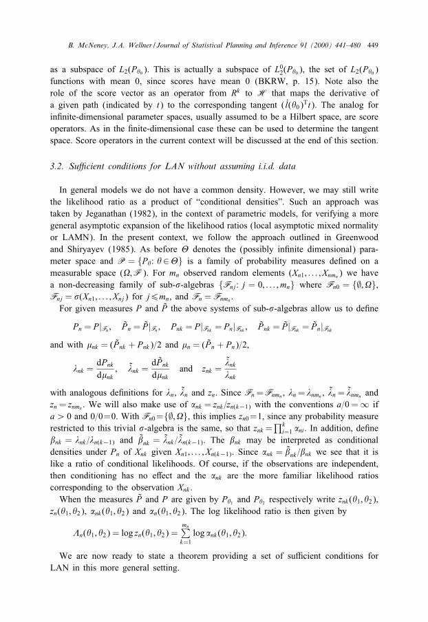
as a subspace of L2(P�0 ). This is actually a subspace of L02(P�0 ), the set of L2(P�0 )functions with mean 0, since scores have mean 0 (BKRW, p. 15). Note also therole of the score vector as an operator from Rk to H that maps the derivative ofa given path (indicated by t) to the corresponding tangent (l(�0)Tt). The analog forin�nite-dimensional parameter spaces, usually assumed to be a Hilbert space, are scoreoperators. As in the �nite-dimensional case these can be used to determine the tangentspace. Score operators in the current context will be discussed at the end of this section.
3.2. Su�cient conditions for LAN without assuming i.i.d. data
In general models we do not have a common density. However, we may still writethe likelihood ratio as a product of “conditional densities”. Such an approach wastaken by Jeganathan (1982), in the context of parametric models, for verifying a moregeneral asymptotic expansion of the likelihood ratios (local asymptotic mixed normalityor LAMN). In the present context, we follow the approach outlined in Greenwoodand Shiryayev (1985). As before � denotes the (possibly in�nite dimensional) para-meter space and P = {P�: �∈�} is a family of probability measures de�ned on ameasurable space (;F). For mn observed random elements (Xn1; : : : ; Xnmn) we havea non-decreasing family of sub-�-algebras {Fnj: j = 0; : : : ; mn} where Fn0 = {∅; },Fnj = �(Xn1; : : : ; Xnj) for j6mn, and Fn =Fnmn .For given measures P and P the above systems of sub-�-algebras allow us to de�ne
Pn = P|Fn ; Pn = P|Fn ; Pnk = P|Fnk = Pn|Fnk ; Pnk = P|Fnk = Pn|Fnk
and with �nk = (Pnk + Pnk)=2 and �n = (Pn + Pn)=2,
�nk =dPnk
d�nk; �nk =
dPnk
d�nkand znk =
�nk
�nk
with analogous de�nitions for �n, �n and zn. Since Fn=Fnmn , �n= �nmn , �n= �nmn andzn = znmn . We will also make use of �nk = znk =zn(k−1) with the conventions a=0 =∞ ifa¿ 0 and 0=0=0. With Fn0={∅; }, this implies zn0=1, since any probability measurerestricted to this trivial �-algebra is the same, so that znk =
∏ki=1 �ni. In addition, de�ne
�nk = �nk=�n(k−1) and �nk = �nk =�n(k−1). The �nk may be interpreted as conditionaldensities under Pn of Xnk given Xn1; : : : ; Xn(k−1). Since �nk = �nk =�nk we see that it islike a ratio of conditional likelihoods. Of course, if the observations are independent,then conditioning has no e�ect and the �nk are the more familiar likelihood ratioscorresponding to the observation Xnk .When the measures P and P are given by P�1 and P�2 respectively write znk(�1; �2),
zn(�1; �2), �nk(�1; �2) and �n(�1; �2). The log likelihood ratio is then given by
�n(�1; �2) = log zn(�1; �2) =mn∑k=1log �nk(�1; �2):
We are now ready to state a theorem providing a set of su�cient conditions forLAN in this more general setting.
450 B. McNeney, J.A. Wellner / Journal of Statistical Planning and Inference 91 (2000) 441–480
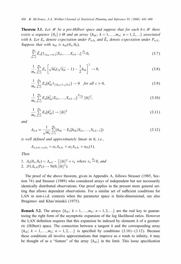
Theorem 3.1. Let H be a pre-Hilbert space and suppose that for each h∈H thereexists a sequence {�n}∈� and an array {hnk ; k = 1; : : : ; mn; n= 1; 2; : : :} associatedwith h. Let En denote expectation under Pn;�0 and En denote expectation under Pn;�n .Suppose that with �nk ≡ �nk(�n; �0);
mn∑k=1
En[1{�nk=∞}|Xn1; : : : ; Xn;k−1]P0→ 0; (3.7)
1mn
mn∑k=1
En
[√mn(
√�nk − 1)− 1
2hnk
]2→ 0; (3.8)
1mn
mn∑k=1
En[h2nk1{|hnk |¿√
n�}]→ 0 for all �¿ 0; (3.9)
1mn
mn∑k=1
En[h2nk |Xn1; : : : ; Xn;k−1]Pn;�0→ ||h||2; (3.10)
1mn
mn∑k=1
En[h2nk ]→ ||h||2 (3.11)
and
�n;h ≡ 1√mn
mn∑i=1(hnk − En[hnk |Xn1; : : : ; Xn;k−1]) (3.12)
is well de�ned and approximately linear in h; i.e.;
�n;a1h1+a2h2 = a1�n;h1 + a2�n;h2 + oP0 (1):
Then
1. �n(�n; �0) = �n;h − 12 ||h||2 + rn where rn
P0→ 0; and2. L(�n;h|P0)→ N(0; ||h||2).
The proof of the above theorem, given in Appendix A, follows Strasser (1985, Sec-tion 74) and Strasser (1989) who considered arrays of independent but not necessarilyidentically distributed observations. Our proof applies in the present more general set-ting that allows dependent observations. For a similar set of su�cient conditions forLAN in non-i.i.d. contexts when the parameter space is �nite-dimensional, see alsoIbragimov and Khas’minskii (1975).
Remark 3.2. The arrays {hnk ; k = 1; : : : ; mn; n = 1; 2; : : :} are the real key to guaran-teeing the right form of the asymptotic expansion of the log likelihood ratios. Howeverthe LAN de�nition requires that this expansion be indexed by elements h of a geomet-ric (Hilbert) space. The connection between a tangent h and the corresponding array{hnk ; k = 1; : : : ; mn; n = 1; 2; : : :} is speci�ed by conditions (3.10)–(3.12). Becausethese conditions all involve approximations that improve as n tends to in�nity, h maybe thought of as a “feature” of the array {hnk} in the limit. This loose speci�cation
B. McNeney, J.A. Wellner / Journal of Statistical Planning and Inference 91 (2000) 441–480 451
of the connection between tangents and the associated arrays leaves a certain amountof freedom in choosing the tangent space in applications. A concrete construction oftangents is given in De�nition 3.5 and this construction is carried out in Examples 2and 3 below.
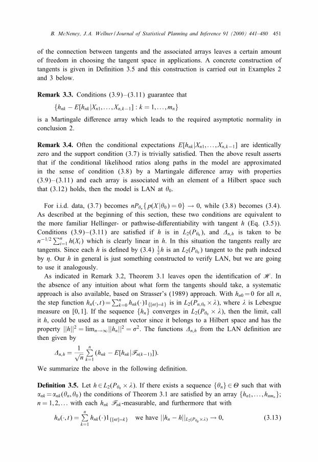
Remark 3.3. Conditions (3.9)–(3.11) guarantee that
{hnk − E[hnk |Xn1; : : : ; Xn;k−1] : k = 1; : : : ; mn}is a Martingale di�erence array which leads to the required asymptotic normality inconclusion 2.
Remark 3.4. Often the conditional expectations E[hnk |Xn1; : : : ; Xn;k−1] are identicallyzero and the support condition (3.7) is trivially satis�ed. Then the above result assertsthat if the conditional likelihood ratios along paths in the model are approximatedin the sense of condition (3.8) by a Martingale di�erence array with properties(3.9)–(3.11) and each array is associated with an element of a Hilbert space suchthat (3.12) holds, then the model is LAN at �0.
For i.i.d. data, (3.7) becomes nP�n{p(X |�0) = 0} → 0; while (3.8) becomes (3.4).As described at the beginning of this section, these two conditions are equivalent tothe more familiar Hellinger- or pathwise-di�erentiability with tangent h (Eq. (3.5)).Conditions (3.9)–(3.11) are satis�ed if h is in L2(P�0 ), and �n;h is taken to ben−1=2
∑ni=1 h(Xi) which is clearly linear in h. In this situation the tangents really are
tangents. Since each h is de�ned by (3.4) 12h is an L2(P�0 ) tangent to the path indexed
by �. Our h in general is just something constructed to verify LAN, but we are goingto use it analogously.As indicated in Remark 3.2, Theorem 3.1 leaves open the identi�cation of H. In
the absence of any intuition about what form the tangents should take, a systematicapproach is also available, based on Strasser’s (1989) approach. With hn0 =0 for all n,the step function hn(·; t)=
∑nk=0 hnk(·)1{[nt]=k} is in L2(Pn;�0 ×�), where � is Lebesgue
measure on [0; 1]. If the sequence {hn} converges in L2(P�0 × �), then the limit, callit h, could be used as a tangent vector since it belongs to a Hilbert space and has theproperty ||h||2 = limn→∞||hn||2 = �2. The functions �n;h from the LAN de�nition arethen given by
�n;h =1√n
n∑k=1(hnk − E[hnk |Fn(k−1)]):
We summarize the above in the following de�nition.
De�nition 3.5. Let h∈L2(P�0 × �). If there exists a sequence {�n}∈� such that with�nk=�nk(�n; �0) the conditions of Theorem 3.1 are satis�ed by an array {hn1; : : : ; hnmn};n= 1; 2; : : : with each hnk Fnk -measurable, and furthermore that with
hn(·; t) =n∑
k=1hnk(·)1{[nt]=k} we have ||hn − h||L2(P�0×�) → 0; (3.13)
452 B. McNeney, J.A. Wellner / Journal of Statistical Planning and Inference 91 (2000) 441–480
then call h the tangent vector corresponding to {�n(h)} ≡ {�n}. The tangent setH0⊂L2(P�0 × �), is the collection of all h as in (3.13).
Although this de�nition does not describe the random variables �n;h explicitly interms of the tangent h (instead they are de�ned implicitly via the array {hnk} associatedwith h) the next proposition shows it is enough to guarantee (approximate) linearity of�n;h in h over any linear subspace of H0. The implication is that the model is LANindexed by such a subspace.
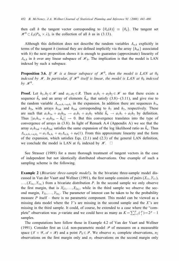
Proposition 3.6. If H is a linear subspace of H0; then the model is LAN at �0indexed by H. In particular; if H0 itself is linear; the model is LAN at �0 indexedby H0.
Proof. Let h1; h2 ∈H and a1; a2 ∈R. Then a1h1 + a2h2 ∈H so that there exists asequence hn and an array of elements hnk that satisfy (3.8)–(3.11), and give rise tothe random variable �n;a1h1+a2h2 in the expansion. In addition there are sequences h1nand h2n with arrays h1nk and h2nk corresponding to h1 and h2, respectively. Theseare such that a1h1n + a2h2n → a1h1 + a2h2 while hn → a1h1 + a2h2 by de�nition.Thus ||a1h1n + a2h2n − hn|| → 0. But this convergence translates into the type ofconvergence of arrays in (3.8). In light of Remark A.4 (Appendix A) we see that thearray a1h1nk+a2h2nk satis�es the same expansion of the log likelihood ratio as hn. Thus�n;a1h1+a2h2 = a1�n;h1 + a2�n;h2 + oP(1). From this approximate linearity and the formof the expansion, which satis�es Eqs. (2.1) and (2.3) of the general LAN de�nition,we conclude the model is LAN at �0 indexed by H.
See Strasser (1989) for a more thorough treatment of tangent vectors in the caseof independent but not identically distributed observations. One example of such asampling scheme is the following.
Example 2 (Bivariate three-sample model). In the bivariate three-sample model dis-cussed in Van der Vaart and Wellner (1991), the �rst sample consists of pairs (X11; Y11);: : : ; (X1n1 ; Y1n1 ) from a bivariate distribution P. In the second sample we only observethe �rst margin, that is X21; : : : ; X2n2 , while in the third sample we observe the sec-ond margin, Y31; : : : ; Y3n3 . The parameter of interest can be taken to be the probabilitymeasure P itself – there is no parametric component. This model can be viewed as amissing data model where the Y ’s are missing in the second sample and the X ’s aremissing in the third sample. It could, of course, be extended to a case where the “com-plete” observation was p-variate and we could have as many as K=
∑pi=1(
pi )=2
p−1samples.The computations here follow those in Example 4:2 of Van der Vaart and Wellner
(1991). Consider �rst an i.i.d. non-parametric model P of measures on a measurablespace (X×Y;A×B) and a point P0 ∈P. We observe n1 complete observations, n2observations on the �rst margin only and n3 observations on the second margin only
B. McNeney, J.A. Wellner / Journal of Statistical Planning and Inference 91 (2000) 441–480 453
giving a total of n observations. It is supposed that each sequence ni=n converges to aknown constant �i with �1 + �2 + �3 = 1.It can be shown that for an arbitrary function g∈G0={all bounded L02(P0) functions},
g is a tangent in the i.i.d. sense corresponding to the path P� given by
P�(A× B) =∫A×B
(1 + �g) dP0
for �∈R small enough so that dP�=dP0 = 1 + �g¿0. Let P�;X and P�;Y denote themarginal probability measures of P�. To compute tangents in these marginal modelswe refer to Proposition A:5 in BKRW which states that the corresponding tangents forthe model where we observe X only is g1(X )=E[g(X; Y )|X ] and when we observe Yonly is g2(Y ) = E[g(X; Y )|Y ].To verify the conditions of Theorem 3.1 suppose the observations are arranged so
that the n1 complete observations come �rst, the n2 observations with X only comesecond, and the n3 observations with Y only come third.For a total sample of size n su�ciently large, take � from the de�nition of the paths
to be n−1=2 and let the array of hnk elements in the nth row be given by
hnk = g1{1; :::; n1}(k) + g11{n1+1;:::;n1+n2}(k) + g21{n1+n2+1;:::;n}(k):
From the independence of the observations we have
�nk =
dP�=dP0 = 1 + �g; 16k6n1;dP�;X =dP0;X = 1 + �g1; n1 + 16k6n1 + n2;dP�;Y =dP0;Y = 1 + �g2; n1 + n2 + 16k6n:
Note that P�.P0, P�;X.P0;X , P�;Y.P0;Y , so that any sequence along such a pathsatis�es (3.7). The above construction emphasizes the three i.i.d. subproblems. Usingthe i.i.d. theory on these subproblems allows straightforward veri�cation of conditions(3.8) and (3.9).The expression in condition (3.10) becomes
n1n
∫g2 dP0 +
n2n
∫g21 dP0;X +
n3n
∫g22 dP0;Y
which converges to �1||g||2 + �2||g1||2 + �3||g3||2 ≡ �2: Thus (3.11) is also satis�edand hence all the necessary conditions for De�nition 3.5 are met. The function hn(·; t)from De�nition 3.5 is
n1∑k=1
g1{[nt]=k} +n2∑k=1
g11{[nt]=k+n1} +n3∑k=1
g21{[nt]=k+n1+n2}
= g1[0; n1=n](t) + g11(n1=n;(n1+n2)=n](t) + g21(n1+n2)=n;1](t):
From the convergence ni=n → �i for all i, and the square integrability of the functiong, the sequence {hn} can be seen to converge in L2(P�0 × �) (or simply L2(P0 × �))to the tangent h(·; t) = g1[0; �1](t) + g11(�1 ;�1+�2](t) + g21(�1+�2 ;1](t). Since the collectionof functions G0 is a linear space and g can be taken to be any member of G0, thecollection of all such h is a linear space. Thus the conclusion is that H0 is linear andhence the model is LAN at P0 indexed by H0.
454 B. McNeney, J.A. Wellner / Journal of Statistical Planning and Inference 91 (2000) 441–480
Another choice for the tangent, as in Van der Vaart and Wellner (1991), would beh= (g; g1; g2) in a space where the inner product is de�ned by
〈h; h〉= �1〈g; g〉+ �2〈g1; g1〉+ �3〈g2; g2〉:Here it is clear how the functions �n;h depend on the tangent vector and it is easilyseen that they are linear in h.
Example 3 (Case-control data). Case-control designs are an e�ective tool for studyingthe relationship between exposures of interest and rare outcomes. Such a design is anexample of a two-sample problem. Let the variable Y indicate case or control statusof an individual with 0 being disease free and 1 being diseased. In addition, suppose acovariate vector X = (X1; : : : ; Xp)′ of exposures and other factors related to disease isavailable. In a common form of the case-control design, covariate information for allor a random sample of subjects who develop disease in a speci�ed “case accession”period of time are recorded, along with the information on a random sample of diseasefree individuals. Let n0 and n1 denote the number in each of the two samples and nthe total number of observations. In this sampling scheme, we obtain realizations fromthe distribution of X conditional on case/control status, while the parameters of interestwill typically be from a prospective model with
Pr(Y = 1|X = x) =exp{�+ X T�}
1 + exp{�+ X T�} :
Here � is an intercept and � is a p-vector of regression, or odds-ratio parameters. Thevector � is of primary interest in this problem. The marginal density g(x) of X is thein�nite-dimensional nuisance parameter in this model.
The parameter space can be described as �×G where �⊂Rp+1 corresponds to theregression parameters and G is the space of distributions for X . The usual approachfor computing variance bounds in the estimation problem involving prospective modelsfor case-control data is to alter the problem slightly so that it is an i.i.d. model. Thei.i.d. modi�cation is given by a two-stage sampling procedure. First, either a case orcontrol is selected with probabilities �1 and �0, respectively, where these probabilitiesare assumed known. Second, the covariate X is sampled for the individual drawn atstep 1. The sample sizes n1 and n0 are now regarded as random. See Breslow andWellner (2000) for recent work establishing the e�ciency of logistic regression forestimating regression parameters in this modi�ed problem. It is widely believed thatvariance bounds obtained for this model are valid in the two-sample model that is usedin practice. In Section 4 we show this to be true, at least when the proportions �1 and�0 are assumed known.The approach for the two-sample version is similar to Example 2 (a three sample
model) in that we use i.i.d. theory to �nd tangents within each of the two samples,and then form the tangents in the sense of De�nition 3.5 based on these. The usualdevelopment is to �rst compute scores in the prospective model, where both diseaseoutcome Y and the covariates X are considered random, and then relate these to the
B. McNeney, J.A. Wellner / Journal of Statistical Planning and Inference 91 (2000) 441–480 455
scores in the retrospective model. Following the calculations in BKRW Section 4:4,we obtain scores at a point ((�; �)0; g0) of the form l(�; �)T�+ a. Here
l(�; �)T�= (X e(Y − E(Y |X ; �; �)))T�;with X e = (1; X T)T, is the score along a path � 7→ (�; �)0 + �� (with �∈Rp+1, �∈R)evaluated at �= 0. The second component a∈L2(G0) (with G0 being the distributionfunction corresponding to the density g0 of the covariates) satis�es∫ [
�−1(√g� −√
g0)− 12a√g0
]2d� → 0 as � ↓ 0
for a path g� through the in�nite-dimensional part of the parameter space.Tangents for the retrospective model are then given by
hi = l(�; �)T�+ a− E(l(�; �)T�+ a|Y = i) ≡ �i(�; a)
for i = 0; 1 corresponding to the control and case samples respectively (BKRW, pp.116–117).Now, suppose the data are arranged so that the controls are listed �rst and then the
cases. Since the tangents h0 and h1 are chosen to satisfy a pathwise-di�erentiabilitycondition like (3.5), the support condition (3.7) is automatically satis�ed, as is condi-tion (3.8). Veri�cation of conditions (3.9)–(3.11) is straightforward and follows thecalculations from Example 2 using the current h0 and h1. We conclude that the tangentin the sense of De�nition 3.5 is
h(·; t) = h01[0; �0](t) + h11(�0 ;1](t) = �0(�; a)1[0; �0](t) + �1(�; a)1(�0 ;1](t) ≡ l�0 (�; a):
The last two expressions emphasize that h is also a function of � and a which determinethe path. Furthermore, the operator l�0 that maps from �; a to h is linear. As a result,the collection of such h as � ranges over Rp+1 and a ranges over L02(G0) is a linearspace which leads to the conclusion, via Proposition 3.6, that the model at ((�; �)0; g0)is LAN indexed by this space. For future reference we also introduce the followingnotation:
l�0 (�; a) = [l(�; �)− E(l(�; �)|Y = 0)1[0; �0](t) + E(l(�; �)|Y = 1)1(�0 ;1](t)]T�+[a− E(a|Y = 0)1[0; �0](t) + E(a|Y = 1)1(�0 ;1](t)]
≡ lT1�+ l2(a): (3.14)
As in Example 2, we note an alternative de�nition of the tangents could be based onh0, h1 and the relative sample sizes �0 and �1 as in the remarks at the end of Example2 above.The above examples all involve independent, but not identically distributed data. For
an application of Theorem 3.1 to a model with dependent observations, see Breslowet al. (2000).As illustrated by Example 3, when the model is speci�ed by a parameterization (other
than the probability measures themselves) the tangent set can often be convenientlydescribed as the range of a linear operator. Because these so-called score operators
456 B. McNeney, J.A. Wellner / Journal of Statistical Planning and Inference 91 (2000) 441–480
play an important role in the di�erentiability conditions in Section 4 we need a moreprecise de�nition.
3.3. Score operators
As we have seen, a natural way to construct tangents at a point in the model is tointroduce a linear operator that acts on tangents to paths in the parameter space. Todescribe paths in a general � that converge to a point �0, we at least need a topology,say �, on �. For convenience let us also assume that � is a vector space and that theoperations of addition and scalar multiplication are continuous under our topology; i.e.(�; �) is a topological vector space. Most often in the study of e�ciency � is eventaken to be a (subset of) a Hilbert space. However, in the following de�nition weleave the structure of � open; all we require is that the dual space of (�; �) separatepoints of � so that adjoints are well de�ned. In the case � is a product space withproduct topology this is true if the dual of each coordinate space separates points ofthat coordinate space (Lemma B.1). It is also true of any normed space.The following is a formal de�nition of the concept of a score operator already used
in the previous section. The notation lin(�) indicates the closed linear span of �.
De�nition 3.7 (Score operators). Let t 7→ �t be a path in � converging to �0 as t ↓ 0with an element �∈ lin(�) such that (�t − �0)=t → � in (�; �) as t ↓ 0. Let � be theset of all � obtained in this way. We say l�0 : � → H is a score operator at �0 iffor all �∈ � there exists a sequence cn ↓ 0 such that �cn forms a sequence �n(h) suchthat Pn;�n(h) has tangent h as in the LAN de�nition (De�nition 2.1) and l�0 (�) = h.
Linearity of � and the score operator imply the image of l�0 is a linear space. Thus,if in addition the random variables �n;h are linear in h, the model is LAN indexed bythe image space.
4. Di�erentiability
In non-parametric models where the parameter of interest is naturally stated asa function of the underlying probability measure, di�erentiability can be establisheddirectly, as in the following.
Example 2 (Cont.). Here we continue with the calculations in Van der Vaart andWellner (1991). In this example the parameter of interest is the probability measure Pitself. To make this a parameter in a Banach space �rst consider a collection of squareintegrable functions F. To simplify matters we might even suppose this collection offunctions is also uniformly bounded since here we are thinking of, for example, thecollection of indicators of measurable sets. Now we may take the Banach space B tobe l∞(F) – the space of all bounded real-valued functions on F. Then the goal may
B. McNeney, J.A. Wellner / Journal of Statistical Planning and Inference 91 (2000) 441–480 457
be stated as estimation of �n(Pn;0) de�ned by
�n(Pn;0) =∫
f(x11; y11) dP0(x11; y11) =1n1
n1∑i=1
∫f(X1i ; Y1i) dP0:
Taking a sequence �n = n−1=2 along a path corresponding to a bounded, measurable,mean 0 function g as speci�ed in Section 3, Example 2, this implies
√n(�n(Pn;�n)− �n(Pn;0)) =
∫gf dP0 =
∫g(f − P0f) dP0;
where Pf=∫f dP and the last equality follows from the fact that g has mean 0. Thus
(2.5) holds with Rn =√n and we can identify �(h) as
�(h)f =⟨1�1(f − P0f; 0; 0); (g; g1; g2)
⟩:
Here we are using the version of the tangent space used in Van der Vaart and Wellner(1991), rather than the version corresponding to De�nition 3.5.To identify the adjoint it su�ces, because B is a function space, to consider the
evaluation maps �f ∈B∗ de�ned by �fb = b(f) for all b∈B. Then the adjoint �T isde�ned by
�f�(h) = �(h)f=⟨1�1(f − P0f; 0; 0); (g; g1; g2)
⟩
=⟨1�1
(f − P0f − af − bf;
�1�2
af;�1�3
bf
); (g; g1; g2)
⟩= 〈�T�f; (g; g1; g2)〉; (4.1)
where af and bf satisfy
E(�2fo(X; Y )− (�1 + �2)af(X )− �2bf(Y )|X = x) = 0
and
E(�3fo(X; Y )− �3af(X )− (�1 + �3)bf(Y )|Y = y) = 0
and fo(X; Y ) ≡ f(X; Y ) − Ef(X; Y ). These last two conditions are derived from thefact that �T must map into H (which is identi�ed with H∗) so that the second elementof �T�f must be the conditional expectation of the �rst given X and the third elementmust be the conditional expectation of the �rst given Y . From these equations it followsthat
Cov(Z(f);Z(g)) = 〈�T�f; �T�g〉=1�1
E(f0−af−bf)(g0 − ag−bg)+1�2
E(afag)+1�3
E(bfbg)
=1�1
E(f0 − af − bf)g0:
The last equality follows from the fact that
− 1�1
E[(f0 − af − bf)ag] =− 1�1
E{E[(f0 − af − bf)|X ]ag}=− 1�1
E{�1�2
afag
}
458 B. McNeney, J.A. Wellner / Journal of Statistical Planning and Inference 91 (2000) 441–480
resulting in some cancellation, with a similar calculation for −1=�1E[(f0−af−bf)bg]resulting in further cancellation.Although these equations characterize the adjoint and provide expressions for the
covariances of in uence functions, we cannot compute these covariances explicitlyexcept in special cases. For instance, under independence, E(a(X )|Y ) = E(a(X )) andE(b(Y )|X )=E(b(Y )). If we choose a(X )=k1E(fo(X; Y )|X ) and b(Y )=k2E(fo(X; Y )|Y )with k1=�2=(�1+�2) and k2=�3=(�1+�3), then E(a(X )|Y )=E(a(X ))=0=E(b(Y ))=E(b(Y )|X ) and it is easily veri�ed that the equations de�ning �T�f hold.Now we may make some calculations of relative e�ciencies along the lines of those
in Bickel et al. (1991). To simplify matters, take the sample space to be [0; 1]× [0; 1]and fst(X; Y ) = 1[0; s](X )1[0; t](Y ) so that fo
st(X; Y ) = 1[0; s](X )1[0; t](Y )− st. In this casewe have a(X ) = k1t(1[0; s](X ) − s) and b(Y ) = k2s(1[0; t](Y ) − t). Direct calculation ofthe variance of �T�f using the formula given above yields
1�1
E(fo2st − affo
st − bffost) =
1�1(st(1− st)− k1t2s(1− s)− k2s2t(1− t));
while the asymptotic variance of the estimator that uses only the complete data isgiven by
1�1
E(fo2) =1�1
st(1− st):
Thus the asymptotic relative e�ciency of the e�cient estimator to the crude esti-mator is
E(fo2st − affo
st − bffost)
E(fo2)=(st(1− st)− k1t2s(1− s)− k2s2t(1− t))
st(1− st):
With �1 ≈ 0 and thus k1 ≈ k2 ≈ 1 this gives a relative e�ciency of approximately(1− s)(1− t)=(1− st) which agrees with Bickel et al. (1991).When �1=�2=�3=1=3 we have k1=k2=1=2 and an ARE of (1−(t+s)=2)=(1−st).
This can be as small as 1=2 (when either s or t are 1) and as big as 1. At t = s=1=2the ARE is 2=3 (cf. with 1=3 when �1 ≈ 0), and when s= t in general we get an AREof (1 + t)−1. We also see that when �1 ≈ 1 we have k1 ≈ k2 ≈ 0 and an ARE ofapproximately 1.
Even when the parameter of interest is speci�ed via a parametrization of the model,it is possible to verify di�erentiability using a “projection of scores” method.
Example 3 (Cont.: Semiparametric models). For semiparametric models when the�nite-dimensional parameter, or some function q of this parameter, is of interest, oneusually proceeds to calculate � via projection of scores. To describe this approachwe adopt the more common notation from semiparametrics. Let now � denote ak-dimensional parameter of interest and g the in�nite-dimensional nuisance parame-ter. Corresponding to these are � and G. In Example 3, for instance, these were givenby Rp+1 and L02(G0), respectively. The space � × G replaces the space � from thede�nition of score operators (De�nition 3.7). In such situations the score operator also
B. McNeney, J.A. Wellner / Journal of Statistical Planning and Inference 91 (2000) 441–480 459
has two components. These were labeled l1 and l2 at the end of Example 3 (Eq.(3.14)), but we now use l� and lg to emphasize the point �; g in the parameter space.The estimation problem, as a function of the probability measures is �(Pn; (�;g))=q(�),
for q : Rk → Rm. A derivative of the form �(lT� �+ lg(a))= q(�)�, where q is the m×k
derivative matrix, satis�es (2.5) with Rn = n1=2. We must, however, identify � as afunction of l
T� �+ lg(a).
First consider projection of the score function l� onto the subspace lg(G). Let
�(·|lg(G)) be the projection operator. For example, we have from Theorem 2 of Ap-pendix 2 of BKRW, that when lg(G) is already closed, the projection of an elementy onto lg(G) is given by
�(y|lg(G)) = lg(lTg lg)
−(lTgy):
where (lTg lg)
−(lTgy) is a solution of (l
Tg lg)x=(l
Tgy): When the inverse (l
Tg lg)
−1 exists,
this is just (lTg lg)
−1(lTgy).
Now let l∗� = l� − �(l�|lg(G)), i.e. the projection of l� onto the orthocomplement
of lg(G), and suppose I∗ = 〈l∗� ; l∗′
� 〉H is non-singular. Then we have
I∗−1〈l∗� ; (l′��+ lg(g))〉H = I∗−1〈l∗� ; l∗
′� �+�(l�|lg(G))′�+ lg(g)〉H
= I∗−1〈l∗� ; l∗′
� �〉H + I∗−1〈l∗� ; �(l�|lg(G))′�+ lg(g)〉H= I∗−1I∗�+ 0= �;
where the 0 term follows from the fact that �(l�|lg(G))′� + lg(g) is in lg(G) while
l∗� is a vector of elements in lg(G)⊥. Thus a candidate for �(·) is 〈qI∗−1l∗� ; ·〉H. The
only concern is that qI∗−1l∗� be a vector of elements in H. This follows from thecalculation
qI∗−1l∗� = qI∗−1l� − qI∗−1�(l�|lg(G));so that the �rst term on the right-hand side is a vector of elements in [l�] and thesecond term is a vector of linear combinations of elements of lg(G) and hence is a
vector of elements of lg(G). Conclude that
qI∗−1l∗� ∈ [l�] + lg(G) =H:
From this point, computation of the adjoint �T is straightforward and we �nd thatfor b∗ in Rm, �Tb∗ = b∗
′I∗−1l∗� which has norm b∗
′I∗−1b∗.
This entire development is completely analogous to the i.i.d. case and when onebegins calculating scores and projections, the similarity with the i.i.d. formulation ofExample 3 becomes apparent. In fact, the information bounds are identical and thereforelogistic regression is still e�cient. This will be shown more formally in the next sectionvia a corollary to the di�erentiability theorem (Theorem 4.1).
Besides the above projection-of-scores approach, another useful method for verifyingdi�erentiability and identifying the adjoint �T in the i.i.d. framework is via a theorem
460 B. McNeney, J.A. Wellner / Journal of Statistical Planning and Inference 91 (2000) 441–480
due to Van der Vaart (1991). The next section describes how this carries over to thepresent context.
4.1. Di�erentiability of implicitly de�ned functionals
Returning to the general notation, we consider estimation of functions of Pn;� of theform
�n(Pn;�) = n(�) (4.2)
for a sequence of maps n from the set � to a Banach space B. Assume there existsa continuous linear map : � → B with
Rn( n(�cn)− n(�))− (�)→ 0 (4.3)
for cn corresponding to a � as in De�nition 3.7. This occurs, for example, if thereexists a map : � → B such that
Rn( (�cn)− (�))− (�)→ 0 as n → ∞and { n} converges to in the sense that
Rn( n(�cn)− (�cn))→ 0 as n → ∞:
Then
limn→∞ Rn( n(�tn)− n(�))
= limn→∞{Rn( n(�tn)− (�tn))− Rn( n(�)− (�)) + Rn( (�cn)− (�))}
and the convergence assumption ensures the limits of the �rst two parts in the right-handside of the above are 0.We further assume there is an N¿0 such that for n¿N , �n is well de�ned. That is,
if Pn;�1 = Pn;�2 , then n(�1) = n(�2).For this discussion we can specialize De�nition 2.2 and de�ne the sequence {�n} to
be di�erentiable if, for any sequence {cn} as in De�nition 3.7 (Section 3),Rn(�n(Pn;�cn )− �n(Pn;�))− �(l(�)) → 0; (4.4)
where � :H → B is continuous and linear. Thus, we wish to identify conditions underwhich �(l(�)) = (�). The theorem to provide such conditions in the i.i.d. case wasgiven in Van der Vaart (1991). With the above notation, the argument at the heart ofhis theorem applies to the present set-up.
Theorem 4.1. Suppose the topology on the space � is chosen so that the dual sepa-rates points (making adjoints well de�ned). Let � be the closed subset of � describedabove and suppose R(i)⊂H⊂R(i): Then the sequence {�n} as in (4:2) is di�eren-tiable in the sense of (2:5) if and only if
R( T)⊂R(l
T):
B. McNeney, J.A. Wellner / Journal of Statistical Planning and Inference 91 (2000) 441–480 461
The adjoint �T is then uniquely speci�ed by the relation
Tb∗ = l
T�Tb∗:
Proof. Proceed as in Van der Vaart (1991). First suppose � exists. By (4.2)–(4.4) wehave that for all � in �
�(l(�)) = limn→∞ Rn(�n(Pn;�cn )− �n(Pn;�)) = lim
n→∞ Rn( n(�cn)− n(�)) = (�):
Hence, for any element b∗ in the dual B∗,
b∗�(l(�)) = b∗ (�) = 〈b∗; (�)〉= 〈 Tb∗; �〉:But, we also have
b∗�(l(�)) = 〈b∗; �(l(�))〉= 〈�Tb∗; l(�)〉= 〈lT�Tb∗; �〉:Since this holds for all �, we conclude that
Tb∗ = l
T�Tb∗ and this is true for all b∗.
Hence R( T)⊂R(l
T). Note that this also implies R(
T)⊥ ⊃R(l
T)⊥.
Now to prove the converse suppose R( T)⊂R(l
T). We may tentatively de�ne � on
R(l) via
�(l(�)) = (�):
That this is well de�ned can be seen as follows. If l(�1)= l(�2), then �1− �2 ∈N(l)=
R(lT)⊥ ⊂R(
T)⊥ =N( ) which implies (�1) = (�2). (The equalities involving
the annihilators are familiar in the case � is a Banach space – cf. Theorem 4:12of Rudin (1991) – but it is straightforward to show they extend to more generaltopological vector spaces given more general de�nitions of adjoints and annihilators.See, for example, the de�nitions in Kelley and Namioka (1963).) We now must show� is continuous and linear. Using the fact that B is a Banach space and Lemma B.2in Appendix B, it su�ces to show it is weakly continuous and linear; that is, for allb∗ ∈B∗, b∗� is a continuous linear functional.By hypothesis,
Tb∗ ∈R(l
T). Let h∗ ∈H∗ be such that
Tb∗ = l
Th∗. Then
b∗�(l(�)) = b∗ (�) = 〈b∗; (�)〉= 〈 Tb∗; �〉= 〈lTh∗; �〉= 〈h∗; l(�)〉= h∗l(�):
Continuity and linearity of h∗ implies the functional b∗� is continuous and linear. Thisconcludes the proof that � is continuous and linear on R(l) and it may be continuouslyextended to H if necessary.To show uniqueness of �T under the condition R(l)⊂H⊂R(l), suppose �T1 and �T2
are two solutions. Then
Tb∗ = l
T�T1b
∗ = lT�T2b
∗
so
�T1b∗ − �T2b
∗ ∈N(lT) =R(l)⊥ =R(l)
⊥ ⊂H⊥:
But �T2b∗ and ��T1b
∗ are both elements of �H and therefore so is the di�erence. Thus�T2b
∗ − �T1b∗ = 0 in H for all b∗ ∈B∗ so that �T2 = �T1 .
462 B. McNeney, J.A. Wellner / Journal of Statistical Planning and Inference 91 (2000) 441–480
Remark 4.2. If the space � can be assumed to be a subspace of a Hilbert space, theconclusion of the theorem can be restated to provide the in uence functions �Tb∗ whichspecify the �nite-dimensional distributions of the optimal limit random variable in the
convolution theorem. Speci�cally, when � is Hilbert, Tcan be thought of as a map
from B∗ to � itself rather than its dual. Similarly, we can think of � as a map fromB∗ to H and interpret l
Tas a map from H to �. Then the in uence functions �Tb∗
are determined by the equation Tb∗ = l
T�Tb∗ where
Tb∗ is the element of � such that
Tb∗h= 〈 Tb∗ ; h〉 for all h∈H. This is how Van der Vaart’s theorem for i.i.d. data is
stated.
Example 1 (Cont). This example provides a simple illustration of the theorem. Herethe tangents were not scores in the quadratic mean sense, as is usually the case, butnevertheless the theorem can be used to check di�erentiability and identify �T. Recallthat in this problem the tangent space was given by H=R(l); the image of the scoreoperator l : R×C0b [0; 1]→ H with l(a; g)=a+g ≡ h for a∈R and g∈C0b [0; 1], wherethe latter is equipped with the supremum norm. Here we take H to be a subspace ofL2(�). It is interesting to note that H is not a closed subspace of L2(�) and hence itis not a Hilbert space. Represent �
∗= (R × C0b [0; 1])
∗ as R × C0b [0; 1]∗; that is, for
�= (a; g); �∗�= �
∗1a+ �
∗2g where �
∗1 ∈R and �
∗2 ∈C0b [0; 1]
∗.
By direct calculation, we �nd the adjoint lT: L2(�)∗ → �
∗, de�ned via
〈h∗; l(�)〉H = 〈lTh∗; �〉�for h∗ ∈H∗, to be given by l
Th∗ = (h∗1; h∗ − h∗1).
To determine if either �(�; f)= � or f(�; f)=f are di�erentiable functionals wemust compute the relevant derivatives and their adjoints. Begin with the functional
�(�; f)=�. This has derivative �(a; g)=a. In this case, the adjoint T� : R→ �
∗is
given by T�b
∗ = (b∗; 0) for all b∗ ∈R. Thus the range of T� is (R× {0}). That this
is contained in the range of lTcan be seen as follows. For any x∈R we can �nd an
h∗x ∈H∗ with h∗x1 = x by taking h∗x (t) = x1[0;1](t). We also have h∗x −∫h∗x = 0 on all
of [0; 1] so that, of course,∫ (h∗x −
∫h∗ d�
)g d�= 0 for g∈C0b [0; 1]:
Thus (R×{0})⊂R(lT) and we conclude from Theorem 4.1 that is di�erentiable. To
compute the lower bound in the convolution theorem we need the adjoint �T : B∗ → H∗
which, according to Theorem 4.1, is given by Tb∗ = l
T�Tb∗. Thus, take �Tb∗ to be
(�Tb∗)h=b∗∫h d�. We might also consider �T as a map from B∗ to H in which case
we would say �Tb∗= �Tb∗ where �Tb∗(t) = b∗1[0;1](t) since then∫�Tb∗(t)h d�= b∗
∫h d�.
From these calculations and the conclusion of Theorem 2.4, it follows that
Cov(b∗1Z; b∗2Z) = 〈�Tb∗1 ; �Tb∗2〉= b∗1b
∗2 ;
B. McNeney, J.A. Wellner / Journal of Statistical Planning and Inference 91 (2000) 441–480 463
that is, the optimal limit random variable has variance 1. This lower bound is achievedby the sample mean �X .If the parameter of interest is f(�; f) = f, another direct calculation shows that,
for b∗ ∈B∗ = C0b [0; 1]∗;
Tfb
∗ = (0; b∗). Thus this operator has range 0 × C0b [0; 1]∗.
However, the form of lTis l
T1 + l
T2 with (l
Th∗)2 g =
∫h∗g d�. The range of l
T2 is a
strict subset of C0b [0; 1]∗ since, for example, the evaluation maps �t(f) = f(t) are in
C0b [0; 1]∗ but cannot be represented as
∫h∗f d� for any h∗. We therefore conclude that
f(�; f) = f is not a di�erentiable function. This is to be expected since it is wellknown (Stone, 1982) that even if smoothness of f is imposed, say by assuming anin�nite number of derivatives, it is not possible to obtain a convergence rate of n−1=2
for estimating an element of (C[0; 1]; || · ||∞).When we use the version of the problem where the nuisance sequence is generated by
the L02(�) function f0, the score operator l is speci�ed by l(a; g)=g+a, now considered
as a map from R× L02(�) to L2(�). Calculation of the adjoint lTin this version of the
model is as before and we �nd that lTis given by l
T1 + l
T2 with (l
Th∗)1 a= a
∫h∗ d�
and (lTh∗)2 g=
∫(h∗ − ∫ h∗ d�)g d�.
For estimating f0(�; f0)= f0, the derivative f0
is a map from R×L02(�) to L02(�).To compute this derivative, it is useful to back up to the de�nition of f. FollowingEq. (4.2), we de�ne
�n(Pn; (�; f)) = n(�; f) = �n(f);
where n(f)(x)= n∫ i=n(i−1)=n f ≡ �ni(f) if x∈ ((i− 1)=n; i=n]. This is reasonable because
we can really only hope to estimate �n(f) based on Xn1; : : : ; Xnn. It is only in the limitthat f enters. Now, from (4.3), using the special choices Rn=
√n and cn=n−1=2, the
derivative is de�ned to be the continuous linear map such that√n( n(�cn ; fcn)− n(�0; f0))− f0
(a; g)→ 0: (4.5)
If we let f0(a; g) = g, the norm of the left-hand side of this expression is
||√n(�n(fcn)− �n(f0))− g||L2(�) = ||√n(�n(fcn − f0))− g||L2(�)= ||√n(�n(g=
√n)− g||L2(�)
= ||�n(g)− g||L2(�) → 0;
where, as noted previously, the convergence to 0 follows from standard results inL2 approximation theory (Royden, 1988). The adjoint may then be computed to be
Tf0g∗ = (0; g∗) for g∗ ∈L02(�)
∗, so that R( Tf0) = ({0} × L02(�))
∗. On the other hand,
the range of lTis (R×L02(�))
∗. To see this, note that every functional in (R×L02(�))∗
is based on an x∈R and an f∈L02(�). Let h∗ =f+ x. For this choice, (l
Th∗)1a= xa
and (lTh∗)2g=
∫fg d�. We conclude that R(
Tf0)⊂R(l
T) and hence by Theorem 4.1,
f0is di�erentiable. The lower bound from the convolution theorem can be calculated
by �rst computing the adjoint �T given by the solution to Tg∗ = l
T�Tg∗ for all
464 B. McNeney, J.A. Wellner / Journal of Statistical Planning and Inference 91 (2000) 441–480
g∗ ∈L02(�)∗. Taking �T to be the identity map from L02 into L2 gives
lT�Tg∗ = l
Tg∗ = (0; g∗) =
Tf0g∗
as required. Thus the in uence functions are simply �Tg∗ = g∗. From Theorem 2.4we conclude that the optimal limit random variable would have covariance functiongiven by
Cov(g∗1Z; g∗2Z) = 〈�Tg∗1 ; �Tg∗2〉L2(�) =
∫g∗1g
∗2 d�:
Unfortunately, a continuous Gaussian process with these marginal distributions does notexist, since, via Sudakov’s inequality (Van der Vaart and Wellner, 1996, PropositionA:2:5), the index set for any continuous process must be totally bounded. This is notthe case for L2(�). Furthermore, according to Proposition 5:5 of Millar (1982, p. 724)there are actually no
√n-consistent estimators in this problem. This illustrates the fact
that di�erentiability of a parameter alone does not guarantee that it can be estimatedat
√n rate. Di�erentiability only allows calculation of the lower bound which asserts
a minimum variance among the class of regular,√n-consistent estimators. It does not
rule out the possibility that this class is empty.As an alternative to the regularity as in De�nition 2.3, we might instead de�ne an
estimator Tn of a B-valued parameter to be weakly e�cient if
b∗(√n(Tn − n(�0; f0)))→d N(0; ||�Tb∗ ||2)
for all b∗ ∈B∗. This is equivalent to the usual notion of e�ciency if B is a �nite-
dimensional space. Such an estimator does exist in this problem, namely ˆf0n(x) =∑ni=1 Xni1((i−1)=n; i=n](x). To see why, �rst recall the notation
�n(f)(x) =n∑
i=1�ni(f) 1((i−1)=n; i=n](x) =
n∑i=1
n∫ i=n
(i−1)=nf d� 1((i−1)=n; i=n](x):
Then for any bounded linear functional g∗ and the function g∗ ∈L02(�) that representsit, we have
g∗(√n( ˆf0n − �n(f0)))
=√ng∗( ˆf0n − �n(f0)) =
√n(∫
g∗ ˆf0n d�−∫
g∗�n(f0) d�)
=√n(
n∑i=1
�ni(g∗)n
(Xni − �ni(f0)))
=n∑
i=1
�ni(g∗)√n(Xni − �ni(f0))
d=N(0; �2n);
where �2n =∑n
i=1 �ni(g∗)2=n. But then
�2n =n∑
i=1�ni(g∗)2
∫ i=n
(i−1)=n1 d�=
n∑i=1
∫ i=n
(i−1)=n�ni(g∗)2 d�
=∫
�2n(g∗) d�= ||�n(g∗)||2 → ||g∗||2:
B. McNeney, J.A. Wellner / Journal of Statistical Planning and Inference 91 (2000) 441–480 465
As a result,
g∗(√n( ˆf0n − �n(f0)))→d N(0; ||g∗||2);
so that it is weakly e�cient. Note however that ˆf0n is not even consistent for �n(f0)in L2(�). We have
|| ˆf0n − �n||2 =n∑
i=1
∫ i=n
(i−1)=n( ˆf0n − �n)2 d�=
1n
n∑i=1(Xni − �ni)2 →p 1
by the WLLN since Xni − �ni ∼ N(0; 1) so the squares are independent �21 withmean 1.
As in Van der Vaart (1991), the di�erentiability theorem may be specialized to thecase of semiparametric models. The results and proofs are identical, but we include thefollowing corollary for completeness. We use the standard semiparametrics notation,introduced earlier in this section, with a k-dimensional parameter of interest � andin�nite-dimensional nuisance parameter g, along with the corresponding score operatorsl� and lg. We consider estimating q(�) with q : Rk → Rm and write q(�) for them× k derivative matrix. As before, the e�cient score for � is de�ned to be l∗� = l� −�(l�| �lg(G)), the projection of l� onto the orthocomplement of �lg(G), and the e�cientinformation matrix is I∗ = 〈l∗� ; l∗
′� 〉H. In this and the following we use the notation a′
for vector transpose of a column vector a to avoid confusion with adjoints.
Corollary 4.3. The sequence �n(Pn;�;g) = q(�) is di�erentiable if and only if N(I∗)⊂N(q(�)T).
Proof. First de�ne n(�; g) ≡ (�; g)=q(�). Let �∈Rk and g∈ G, where G is the spaceof derivatives in the in�nite-dimensional part of the parameter space and g correspondsto a path {gt : t ¿ 0} with g= g0. Then
(�; g) = limt↓0( (�+ t�; gt)− (�; g)) = lim
t↓0(q(�+ t�; gt)− q(�)) = q(�)�:
Thus we have, for any b∗ ∈B∗=Rm; 〈 (�; g); b∗〉B=〈(�; g); Tb∗〉Rk×G so that Tb∗=
(b∗′q(�); 0). In other words, R(
T) = (R(q(�)T); {0}).
The score operator l is given by l(�; g) = l′��+ lgg so that for any h∈H,
〈l(�; g); h〉H = 〈l′��+ lgg; h〉H = 〈l′��; h〉H + 〈lgg; h〉H = 〈l′�; h〉H�+ 〈g; lTg h〉Gand hence
lTh= (l
T� h; l
Tg h) = (〈l
′�; h〉H; l
Tg h):
Thus, according to Theorem 4.1, the parameter is di�erentiable if and only if
R(q(�)T)⊂{〈l′�; h〉H: h∈N(lg) =R(lg)⊥}:
466 B. McNeney, J.A. Wellner / Journal of Statistical Planning and Inference 91 (2000) 441–480
Since R(lg)⊥ is spanned by the e�cient score l∗� , any h∈R(lg)⊥ is of the formh= l∗
′� a, and consequently
〈l′�; h〉H = 〈l∗� ; h〉H = 〈l∗� ; l∗′
� 〉H = I∗a:
Thus the parameter is di�erentiable if and only if R(q(�)T)⊂R(I∗). Finally, becausethe two ranges in question are �nite-dimensional and hence closed, this last statementis equivalent to the condition of the corollary.
Note that for estimating all of �, q is the identity, and the corollary states that �is di�erentiable if and only if the e�cient score matrix is non-singular. This was thecondition used in the projection-of-scores approach earlier in this section.In addition to the above specialization of Theorem 4.1 we have the following corol-
lary giving su�cient conditions for equivalence of information bounds in di�erentexperiments. This can be used, for example, to show that the variance bounds are thesame for the case-control example (Example 3) as in its randomized i.i.d. version.
Corollary 4.4. Consider two di�erent LAN experiments that involve the same param-eter space and for which the goal is estimation of the same parameter in a Banachspace B. Suppose the �rst experiment is LAN indexed by H1 and the second LANindexed by H2. Let l1 : � → H1 denote the score operator for the �rst experi-ment and l2 : � → H2 the score operator for the second where R(l1) =H1 andR(l2) =H2. If the map � : H1 → H2 de�ned by l2� = �l1� is a (Hilbert space)isomorphism then the parameter is di�erentiable in one experiment if and only if it isdi�erentiable in the other. If the parameter is di�erentiable; the information boundsare the same in the two experiments.
Proof. The function of the parameter is hypothesized to be the same for both ex-
periments and hence so is T. From the de�nition of � and the fact that it is an
isomorphism (which means that � is a one-to-one mapping of H1 onto H2 whichsatis�es 〈�g; �h〉H2 = 〈g; h〉H1 for all g; h∈H1; see e.g. Rudin (1966, p. 86) we �ndthat
〈�; lT1h1〉� = 〈l1�; h1〉H1 = 〈�−1l2�; h1〉H1 = 〈l2�; �h1〉H2 = 〈�; lT2�h1〉�:
Thus lT1 = l
T2� and similarly l
T2 = l
T1�
−1. Suppose � ∗ ∈R(lT1 ). Then � ∗= l
T1h1 for some
h1 ∈H1. Setting h2 = �h1, we have
lT1h1 = l
T1�h2 = l
T2h2
so that � ∗ ∈R(lT2 ). Hence R(l
T1 )⊂R(l
T2 ). A similar argument shows the reverse in-
clusion so that R(lT1 ) =R(l
T2 ). By Theorem 4.1 we conclude that a parameter will be
di�erentiable in one model if and only if it is di�erentiable in the other.Next let �i :Hi → B and �Ti : B
∗ → Hi ; i=1; 2 be the derivatives of the functionalsto be estimated and their adjoints for the two experiments. That �T2 =� ◦ �T1 follows in
B. McNeney, J.A. Wellner / Journal of Statistical Planning and Inference 91 (2000) 441–480 467
a similar manner to the proof of uniqueness of �T in Theorem 4.1. In particular, wehave from Theorem 4.1 that for any b∗ ∈B∗
Tb∗ = l
T1 �T1b
∗ = lT2��T1b
∗ = lT2 �T2b
∗:
Thus,
�T2b∗ − ��T1b
∗ ∈N(lT2 ) =R(l2)⊥ =H⊥
2 :
We conclude that �T2b∗ −��T1b
∗ = 0 in H2 for all b∗ ∈B∗ so that �T2 =��T1 , or equiv-alently, �T1 = �−1�T2 . Finally, using again the fact that � is an isomorphism,
〈�T1b∗1 ; �T1b∗2〉H1 = 〈�T2b∗1 ; �T2b∗2〉H2
and the optimal limit Z0 has the same covariance function under either experiment.
Example 3 (Cont). In either the example or its randomized version the goal is stillthe estimation of the regression parameters �. Compare the score operator
l�0 (�; a)(·; t) = (lT1�)(·; t) + (l2(a))(·; t) = �0(�; a)1[0; �0](t) + �1(�; a)1(�0 ;1](t)
given in Section 3 to the score operator for the i.i.d. version speci�ed in BKRW onp. 116 as li:i:d:(�; a)(·; i) = �i(�; a). Label the former as experiment 1 and the secondas experiment 2. Then it is easily veri�ed that the map � is an isomorphism since
〈l�0 (�1; a1); l�0 (�2; a2)〉H1 =∫ ∫ 1
0l�0 (�1; a1)l�0 (�2; a2) dt dP�0
=∫
1∑i=0
�i�i(�1; a1)�i(�2; a2) dP�0 ;
while
〈li:i:d:(�1; a1); li:i:d:(�2; a2)〉H2 =∫
1∑i=0
�i�i(�1; a1)�i(�2; a2) dP�0
as well.Thus, the information bound is the same in Example 3 as in the i.i.d. version. As
shown in Breslow and Wellner (2000) logistic regression is an e�cient estimator forthe regression parameters in the latter and hence in the two sample version of Example3 as well.
The above program has also been carried out for response-selective sampling designs;see Breslow et al. (2000).
5. Regularity and linearity of estimators
In this section, the goal is to develop the notions of regularity and linearity ofestimators, and to connect these with the geometry of the tangent space. The �rst task
468 B. McNeney, J.A. Wellner / Journal of Statistical Planning and Inference 91 (2000) 441–480
is to establish an analog to Proposition 3.3.1 of BKRW, part of which states that anasymptotically linear and regular estimator with in uence function in the tangent spaceis e�cient. For this we need an analogous de�nition of linearity of an estimator. Onepossibility is to say an estimator Tn is asymptotically linear if for all b∗ ∈B∗,
√nb∗(Tn − �n(Pn;�0 )) = �n;hb∗ + oP(1)
for some hb∗ . The problem here is that �n;h is, in general, only de�ned on H. Notethat in the i.i.d. setting, the map �n;h is de�ned to be
�n;h = n−1=2n∑
i=1h(Xi)
for h∈ P⊂L2(P�0 ). In this case it is clear how to extend �n;h to all of L2(P�0 ) andwe obtain a useful de�nition of asymptotic linearity. Without being able to extend�n;h in some meaningful way, the resulting de�nition would declare an estimator to beasymptotically linear only if it had in uence function in the tangent space, in whichcase asymptotically linear and regular would be a synonym for e�cient. This is onlythe case in the i.i.d. theory when treating a fully nonparametric model.There are several possibilities for extending �n;h. For instance, following Bickel
(1993, p. 67) one could de�ne a tangent space and maps �n;h on a “largest possible”model of interest M . Then the �n;h described in this paper would be the restriction tothe tangent space H of particular interest. This largest model corresponds to a fullynonparametric model in the i.i.d. theory.Alternatively, we could proceed based on the results of Theorem 3.1 and in particular
the condition (3.12) which states
�n;h ≡ 1√mn
mn∑i=1(hnk − En[hnk |Xn1; : : : ; Xn;k−1])
is well de�ned and approximately linear in h; i.e., �n;a1h1+a2h2 =a1�h1 +a2�h2 +oP0(1).The array {hnk} above is required to approximate the array of conditional log-likelihoodratios {�nk}, but �n;h remains perfectly well de�ned for arbitrary arrays, say subject tothe constraint that each hnk is square integrable. This is still a rather vague de�nition.To go one step further, the de�nition could be based on the particular form of tangentvectors h de�ned in De�nition 3.5 based on building step functions
hn(·; t) =n∑
k=1hnk(·)1{[nt]=k} and requiring ||hn − h||L2(P�0×�) → 0:
The tangent vectors constructed in this way are also in the spirit of Bickel (1993); seehis Example 2:5:2, p. 68.For now, the simplest approach appears to be to specify a largest model of interest
M . Corresponding to M , let HM denote the tangent space and suppose �n;h is wellde�ned and linear on HM . In what follows assume HM is closed.
De�nition 5.1 (Asymptotic linearity). Let �n : Pn → B be a sequence of parameterstaking values in a Banach space B and Tn be a sequence of estimators for �n. We say
B. McNeney, J.A. Wellner / Journal of Statistical Planning and Inference 91 (2000) 441–480 469
Tn is asymptotically linear if for all b∗ ∈B∗,√nb∗(Tn − �n(Pn;�0 )) = �n;hb∗ + oP(1)
for hb∗ ∈HM and the associated array �n;hb∗ as in the LAN de�nition (De�nition2.1) for the largest model of interest M . In particular, if �n(Pn;�) is an m-dimensionalparameter (m¡∞), a sequence {Tn} is asymptotically linear if
√n(Tn − �(P�0 )) = �n; h + oP(1)
for h= (h1; : : : ; hm)∈HmM and the associated �n; h = (�n; h1 ; : : : ; �n; hm).
Remark 5.2. Even in the i.i.d. theory there are several possible de�nitions of asymp-totic linearity for estimators of a general parameter (all of which coincide when theparameter is �nite-dimensional). See, for example, De�nition 5:2:5 of BKRW (p. 180).The above choice corresponds to their weakly asymptotically linear.
The �rst proposition uses the specialized form of the asymptotic linearity de�nitionfor �nite-dimensional parameters. The second is a result for the general case. In viewof Remark 5.2, it seems helpful to have separate results for the �nite-dimensional andgeneral cases.
Proposition 5.3. Suppose the model is LAN at a point �0 indexed by a subspaceH of a Hilbert space and that the maps �n;h of De�nition 2:1 are linear in h. Let�n(Pn;�) be a sequence of m-dimensional parameters that are pathwise di�erentiablewith derivative represented by �∈ �H
m. If {Tn} is asymptotically linear in �n; h then
it is regular if and only if (h− �)⊥Hm. If h∈ �Hmthen {Tn} is regular if and only
if h= � in which case Tn is e�cient.
Proof. Let Pn;0 ≡ Pn;�0 . For an h∈H, consider its LAN sequence {�n(h)}. Then bylinearity of �n;h in h on all of HM , LAN, and the Cram�er–Wold device it follows thatunder Pn;0(√
n(Tn − �n(Pn;0))�n(�n(h); �0)
)=(
�n; h + oP(1)�n;h − 1
2�22 + oP(1)
)→d N
((0
−�22=2
); �)
;
where �= [�ij], �11 = [〈hi; hj〉HM ], �12 = 〈h; h〉HM , and �22 = ||h||HM .Then, by Le Cam’s third lemma (see, for example, Van der Vaart and Wellner,
1996, pp. 404–405)√n(Tn − �n(Pn;0))→d N(�12; �11)
under Pn;�n(h). Also,√n(�n(Pn;�n(h))− �n(Pn;0))→ �(h) = 〈h; �〉HM for �∈ �H
m ⊂ �HmM :
Combining these two facts with√n(Tn − �n(Pn;�n(h))) =
√n(Tn − �n(Pn;0))−
√n(�n(Pn;�n(h))− �n(Pn;0))
470 B. McNeney, J.A. Wellner / Journal of Statistical Planning and Inference 91 (2000) 441–480
implies that under Pn;�n(h)√n(Tn − �n(Pn;�n(h)))→d N(�12 − �(h); �11) = N(〈h; h− �〉HM ; �11):
Hence Tn is regular if and only if 〈h; h − �〉HM is constant for all h. Since 0∈H itmust be that this constant is 0, which implies that (h− �)⊥H (coordinatewise). If, inaddition, h∈ �H
m, then h− � is in �H
m, while also being orthogonal to H and �H. This
implies that h − � = 0; i.e. h = �. Thus the asymptotic variance of√n(Tn − �n(Pn;)))
is that of �n; � which is 〈�T; �〉; the information bound. In other words, Tn is e�cient.
Proposition 5.4. Suppose the model is LAN at a point �0 indexed by a subspaceH of a Hilbert space and that the maps �n;h of De�nition 2:1 are linear in h. Let�n(Pn;�) be a sequence of B-valued parameters that are pathwise di�erentiable withderivative � such that b∗� can be represented by a �b∗ ∈ �H for all b∗ ∈B∗. If {Tn} isasymptotically linear in the sense of De�nition 5:1; with all hb∗ ∈H; then {b∗Tn} isregular if and only if (hb∗ − �b∗)⊥H. If; in addition;
√n(Tn − �n(Pn;�n(h))) converges
weakly under {Pn;�n(h)} to a tight limit in B for each {�n(h)}; then {Tn} is regular.When hb∗ ∈H; then {b∗Tn} is regular if and only if hb∗= �b∗ in which case {b∗Tn}
is e�cient for b∗�n(Pn;0). Similarly; if√n(Tn − �n(Pn;�n(h))) converges weakly under
{Pn;�n(h)} to a tight limit in B for each {�n(h)}; then {Tn} is regular and e�cient.
Proof. The assertions regarding regularity and e�ciency of b∗Tn follow from Propo-sition 5.3. If b∗Tn is regular and e�cient for all b∗ ∈B, then with the additionalassumption of weak convergence of
√n(Tn − �n(Pn;�n(h))) under {Pn;�n(h)}, conclude
that this limit must be the same for all {�n(h)} so that {Tn} is regular.When b∗Tn is regular and e�cient for all b∗ ∈B, then the additional assumption of
weak convergence implies√n(Tn − �n(Pn;�n(h))) has the same covariance function as
the optimal limit random element. That is, Tn is regular and e�cient.
Example 2 (Cont.). In the bivariate three sample model, the natural way to obtaina largest possible model of interest would be to drop the restriction that the secondsample is from the �rst margin (X ) of the bivariate distribution P0 ≡ P01 and thatthe third sample is from the second margin (Y ). The second and third samples couldinstead be drawn from measures P02 and P03 where P0i.P01, i=2; 3. This larger modelwould lead to tangents of the form (g1; g2; g3) in a space HM with inner-product
〈h; h〉HM =3∑
i=1�i〈gi; gi〉L2(P01);
where now g2 need not be E(g1|X ) and g3 need not be E(g1|Y ); these are the restric-tions that hold true on the subspace H corresponding to the model of interest. It canbe shown that the maps �n;h on the larger space HM are of the form
1√n
3∑j=1
nj∑i=1
gj(Xji; Yji):
B. McNeney, J.A. Wellner / Journal of Statistical Planning and Inference 91 (2000) 441–480 471
The naive estimator of P01 just uses the n1 observations from the �rst sample; i.e.
P01 = Pn1 =1n1
n1∑i=1
�(X1i ; Y1i):
For the purpose of estimation, P01 is considered to be an element of ‘∞(F) whereF is a given collection of P01-square-integrable functions. Because this is a functionspace, it su�ces to consider only �f ∈ ‘∞(F)∗ for a given f∈F, where �f(b)=b(f)for all b∈B ≡ ‘∞(F). By de�nition Pn1 is asymptotically linear if for all �f
√n(�fPn1 − �fP01) =
√n(Pn1f − P01f) =
√n1n1
n1∑i=1(f(Xi1; Y1i)− P01f)
=1√n
n1∑i=1
nn1(f(Xi1; Y1i)− P01f) = �n;h�f
for some h�f ∈HM , at least up to an oP(1) term. This is true for h�f = �−11 (f −P01f; 0; 0).From Van der Vaart and Wellner’s calculations, as described earlier in Section 4,
the element of H that represents the derivative �f� is
��f =1�1
(f − P01f − af − bf;
�1�2
af;�1�3
bf
);
where af and bf satisfy
E(�2fo(X; Y )− (�1 + �2)af(X )− �2bf(Y )|X = x) = 0
and
E(�3fo(X; Y )− �3af(X )− (�1 + �3)bf(Y )|Y = y) = 0
with fo(X; Y ) = f(X; Y ) − Ef(X; Y ). Recall that these two conditions were derivedfrom the fact that the second element of ��f must be the conditional expectation ofthe �rst given X and the third element must be the conditional expectation of the �rstgiven Y .From the de�nition of ��f and the calculations in Eq. (4.1) we see that
〈h�f ; (g1; g2; g3)〉HM = 〈��f ; (g1; g2; g3)〉HM or 〈h�f − ��f ; (g1; g2; g3)〉HM = 0
for any (g1; g2; g3)∈H. Hence �fPn1 =Pn1f is a regular (but not e�cient) estimatorof �fP01 =P01f. Finally, if we assume F is such that supf∈F||Pn;�nf
2||=O(1), thenTheorem 3:10:12 of Van der Vaart and Wellner (1996, p. 407) implies
√n(Pn1−Pn;�n)
converges weakly under Pn;�n . Thus Proposition 5.4 implies that Pn1 is regular. (Notethat Theorem 3:10:12 of Van der Vaart and Wellner (1996) may be used to showregularity of Pn1 without Proposition 5.4. However, the above calculation provides anillustration of the geometric content of this proposition.)
6. Discussion of open problems
Although several results used in application of convolution theorems for i.i.d. datahave been extended to non-i.i.d. models, many others remain. For instance, a nice
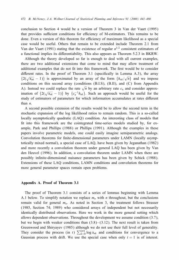
472 B. McNeney, J.A. Wellner / Journal of Statistical Planning and Inference 91 (2000) 441–480
conclusion to Section 4 would be a version of Theorem 3 in Van der Vaart (1995)that provides su�cient conditions for e�ciency of M-estimators. This remains to bedone. Even a version of this theorem for e�ciency of maximum likelihood as a specialcase would be useful. Others that remain to be extended include Theorem 2:1 fromVan der Vaart (1991) stating that the existence of regular n1=2 consistent estimators ofa functional implies its di�erentiability. This also appears as Theorem 5:2:3 in BKRW.Although the theory developed so far is enough to deal with all current examples,
there are two additional extensions that come to mind that may allow treatment ofadditional examples that do not �t into this framework. The �rst would be to considerdi�erent rates. In the proof of Theorem 3.1 (speci�cally in Lemma A.3), the array{2(√�nk − 1)} is approximated by an array of the form {hnk=
√n} and we impose
conditions on this second array (conditions (B.I.S), (B.II), and (C) from AppendixA). Instead we could replace the rate
√n by an arbitrary rate cn and consider approx-
imation of {2(√�nk − 1)} by {c−1n hnk}. Such an approach would be useful for thestudy of estimators of parameters for which information accumulates at rates di�erentthan n.A second possible extension of the results would be to allow the second term in the
stochastic expansion of the log likelihood ratios to remain random. This is a so-calledlocally asymptotically quadratic (LAQ) condition. An interesting class of models that�t into this framework are the cointegrated time-series models studied by, for ex-ample, Park and Phillips (1988) or Phillips (1991). Although the examples in thesepapers involve parametric models, one could easily imagine semiparametric analogs.Convolution theorems for �nite-dimensional parameters under LAMN (locally asymp-totically mixed normal), a special case of LAQ, have been given by Jeganathan (1982)and more recently a convolution theorem under general LAQ has been given by Vanden Heuvel (1996). In addition, a convolution theorem under LAMN when there arepossibly in�nite-dimensional nuisance parameters has been given by Schick (1988).Extensions of these LAQ conditions, LAMN conditions and convolution theorems formore general parameter spaces remain open problems.
Appendix A. Proof of Theorem 3.1
The proof of Theorem 3.1 consists of a series of lemmas beginning with LemmaA.1 below. To simplify notation we replace mn with n throughout, but the conclusionsremain valid for general mn. As noted in Section 3, the treatment follows Strasser(1985, Section 74; 1989) who considered arrays of independent but not necessarilyidentically distributed observations. Here we work in the more general setting whichallows dependent observations. Throughout the development we assume condition (3.7),but we begin with weaker conditions than (3.8)–(3.12). The next result is taken fromGreenwood and Shiryayev (1985) although we do not use their full level of generality.They consider the process (in t)
∑[nt]k=0 log �nk and conditions for convergence to a
Gaussian process with drift. We use the special case when only t = 1 is of interest.
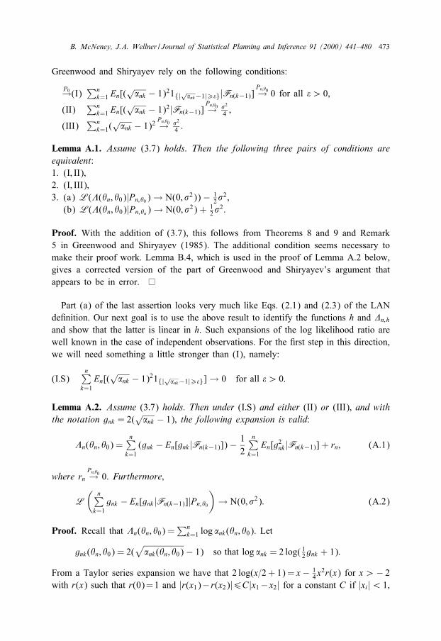
B. McNeney, J.A. Wellner / Journal of Statistical Planning and Inference 91 (2000) 441–480 473
Greenwood and Shiryayev rely on the following conditions:
P0→(I) ∑nk=1 En[(
√�nk − 1)21{|√�nk−1|¿�}|Fn(k−1)]
Pn;�0→ 0 for all �¿ 0,
(II)∑n
k=1 En[(√�nk − 1)2|Fn(k−1)]
Pn;�0→ �2
4 ;
(III)∑n
k=1(√�nk − 1)2
Pn;�0→ �2
4 :
Lemma A.1. Assume (3:7) holds. Then the following three pairs of conditions areequivalent:1. (I; II);2. (I; III);3. (a) L(�(�n; �0)|Pn;�0 )→ N(0; �2))− 1
2�2,
(b) L(�(�n; �0)|Pn;�n)→ N(0; �2) + 12�2.
Proof. With the addition of (3.7), this follows from Theorems 8 and 9 and Remark5 in Greenwood and Shiryayev (1985). The additional condition seems necessary tomake their proof work. Lemma B.4, which is used in the proof of Lemma A.2 below,gives a corrected version of the part of Greenwood and Shiryayev’s argument thatappears to be in error.
Part (a) of the last assertion looks very much like Eqs. (2.1) and (2.3) of the LANde�nition. Our next goal is to use the above result to identify the functions h and �n;h
and show that the latter is linear in h. Such expansions of the log likelihood ratio arewell known in the case of independent observations. For the �rst step in this direction,we will need something a little stronger than (I), namely:
(I:S)n∑
k=1En[(
√�nk − 1)21{|√�nk−1|¿�}]→ 0 for all �¿ 0:
Lemma A.2. Assume (3:7) holds. Then under (I:S) and either (II) or (III); and withthe notation gnk = 2(
√�nk − 1); the following expansion is valid:
�n(�n; �0) =n∑
k=1(gnk − En[gnk |Fn(k−1)])− 1
2
n∑k=1
En[g2nk |Fn(k−1)] + rn; (A.1)
where rnPn;�0→ 0. Furthermore;
L
(n∑
k=1gnk − En[gnk |Fn(k−1)]|Pn;�0
)→ N(0; �2): (A.2)
Proof. Recall that �n(�n; �0) =∑n
k=1 log �nk(�n; �0). Let
gnk(�n; �0) = 2(√
�nk(�n; �0)− 1) so that log �nk = 2 log( 12gnk + 1):
From a Taylor series expansion we have that 2 log(x=2+ 1)= x− 14x2r(x) for x¿− 2
with r(x) such that r(0)=1 and |r(x1)− r(x2)|6C|x1−x2| for a constant C if |xi|¡ 1,
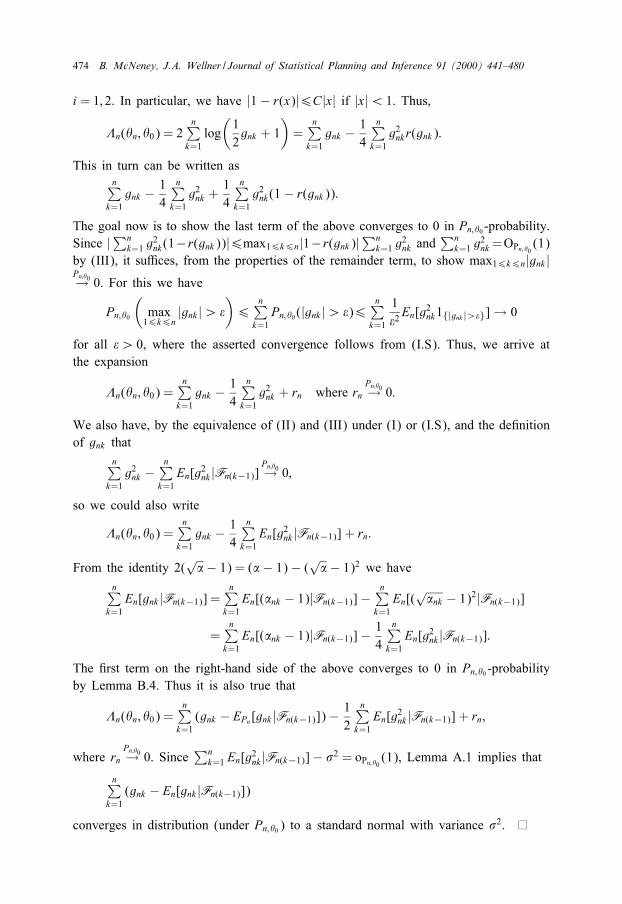
474 B. McNeney, J.A. Wellner / Journal of Statistical Planning and Inference 91 (2000) 441–480
i = 1; 2. In particular, we have |1− r(x)|6C|x| if |x|¡ 1. Thus,
�n(�n; �0) = 2n∑
k=1log(12gnk + 1
)=
n∑k=1
gnk − 14
n∑k=1
g2nkr(gnk):
This in turn can be written asn∑
k=1gnk − 1
4
n∑k=1
g2nk +14
n∑k=1
g2nk(1− r(gnk)):
The goal now is to show the last term of the above converges to 0 in Pn;�0 -probability.Since |∑n
k=1 g2nk(1−r(gnk))|6max16k6n|1−r(gnk)|
∑nk=1 g
2nk and
∑nk=1 g
2nk=OPn; �0 (1)
by (III), it su�ces, from the properties of the remainder term, to show max16k6n|gnk |Pn;�0→ 0. For this we have
Pn;�0
(max16k6n
|gnk |¿�)6
n∑k=1
Pn;�0 (|gnk |¿�)6n∑
k=1
1�2
En[g2nk1{|gnk |¿�}]→ 0
for all �¿ 0, where the asserted convergence follows from (I.S). Thus, we arrive atthe expansion
�n(�n; �0) =n∑
k=1gnk − 1
4
n∑k=1
g2nk + rn where rnPn;�0→ 0:
We also have, by the equivalence of (II) and (III) under (I) or (I.S), and the de�nitionof gnk that
n∑k=1
g2nk −n∑
k=1En[g2nk |Fn(k−1)]
Pn;�0→ 0;
so we could also write
�n(�n; �0) =n∑
k=1gnk − 1
4
n∑k=1
En[g2nk |Fn(k−1)] + rn:
From the identity 2(√�− 1) = (�− 1)− (√�− 1)2 we have
n∑k=1
En[gnk |Fn(k−1)] =n∑
k=1En[(�nk − 1)|Fn(k−1)]−
n∑k=1
En[(√�nk − 1)2|Fn(k−1)]
=n∑
k=1En[(�nk − 1)|Fn(k−1)]− 1
4
n∑k=1
En[g2nk |Fn(k−1)]:
The �rst term on the right-hand side of the above converges to 0 in Pn;�0 -probabilityby Lemma B.4. Thus it is also true that
�n(�n; �0) =n∑
k=1(gnk − EPn [gnk |Fn(k−1)])− 1
2
n∑k=1
En[g2nk |Fn(k−1)] + rn;
where rnPn;�0→ 0. Since
∑nk=1 En[g2nk |Fn(k−1)]− �2 = oPn; �0 (1), Lemma A.1 implies that
n∑k=1(gnk − En[gnk |Fn(k−1)])
converges in distribution (under Pn;�0 ) to a standard normal with variance �2.
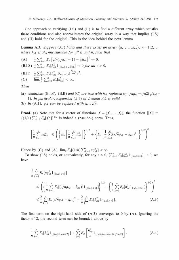
B. McNeney, J.A. Wellner / Journal of Statistical Planning and Inference 91 (2000) 441–480 475
One approach to verifying (I.S) and (II) is to �nd a di�erent array which satis�esthese conditions and also approximates the original array in a way that implies (I.S)and (II) hold for the original. This is the idea behind the next lemma.
Lemma A.3. Suppose (3:7) holds and there exists an array {hn1; : : : ; hnn}; n=1; 2; : : :where hnk is Fnk -measurable for all k and n; such that
(A) 1n
∑nk=1 En
[√n(√�nk − 1)− 1
2hnk]2 → 0;
(B:I:S) 1n
∑nk=1 En[h2nk1{|hnk |¿
√n�}]→ 0 for all �¿ 0;
(B:II) 1n
∑nk=1 En[h2nk |Fn(k−1)]
Pn;�0→ �2;
(C) limn1n
∑nk=1 En[h2nk ]¡∞:
Then
(a) conditions (B:I:S); (B:II) and (C) are true with hnk replaced by√ngnk=
√n2(
√�nk−
1). In particular; expansion (A:1) of Lemma A:2 is valid.(b) In (A:1); gnk can be replaced with hnk=
√n.
Proof. (a) Note that for a vector of functions f = (f1; : : : ; fn), the function ||f|| ≡{(1=n)∑n
k=1 En[f2k ]}1=2 is indeed a (pseudo-) norm. Thus,
[1n
n∑k=1
ng2nk
]6
({En
[1n
n∑k=1
h2nk
]}1=2+{En
[1n
n∑k=1(√ngnk − hnk)2
]}1=2)2:
Hence by (C) and (A), limn En[(1=n)∑n
k=1 ng2nk ]¡∞.
To show (I:S) holds, or equivalently, for any �¿ 0,∑n
k=1 En[g2nk1{|gkn|¿�}]→ 0, wehave
1n
n∑k=1
En[ng2nk1{|gnk |¿�}]
6
({1n
n∑k=1
En[(√ngnk − hnk)21{|gkn|¿�}]
}1=2+{1n
n∑k=1
En[h2nk1{|gnk |¿�}]}1=2)2
62n
n∑k=1
En[√ngnk − hnk ]2 +
2n
n∑k=1
En[h2nk1{|gnk |¿�}]: (A.3)
The �rst term on the right-hand side of (A.3) converges to 0 by (A). Ignoring thefactor of 2, the second term can be bounded above by
1n
n∑k=1
En[h2nk1{|hnk |¿√
n�=2}] +n∑
k=1En
[h2nkn1{|√ngnk−hnk |¿
√n�=2}
]: (A.4)
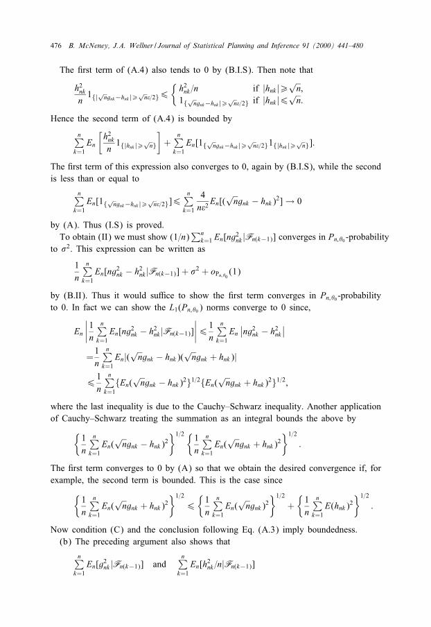
476 B. McNeney, J.A. Wellner / Journal of Statistical Planning and Inference 91 (2000) 441–480
The �rst term of (A.4) also tends to 0 by (B.I.S). Then note that
h2nkn1{|√ngnk−hnk |¿
√n�=2}6
{h2nk =n if |hnk |¿
√n;
1{√ngnk−hnk |¿√
n�=2} if |hnk |6√n:
Hence the second term of (A.4) is bounded by
n∑k=1
En
[h2nkn1{|hnk |¿
√n}
]+
n∑k=1
En[1{√ngnk−hnk |¿√
n�=2}1{|hnk |¿√
n}]:
The �rst term of this expression also converges to 0, again by (B.I.S), while the secondis less than or equal to
n∑k=1
En[1{√ngnk−hnk |¿√
n�=2}]6n∑
k=1
4n�2
En[(√ngnk − hnk)2]→ 0
by (A). Thus (I.S) is proved.To obtain (II) we must show (1=n)
∑nk=1 En[ng2nk |Fn(k−1)] converges in Pn;�0 -probability
to �2. This expression can be written as
1n
n∑k=1
En[ng2nk − h2nk |Fn(k−1)] + �2 + oPn; �0 (1)
by (B:II). Thus it would su�ce to show the �rst term converges in Pn;�0 -probabilityto 0. In fact we can show the L1(Pn;�0 ) norms converge to 0 since,
En
∣∣∣∣1nn∑
k=1En[ng2nk − h2nk |Fn(k−1)]
∣∣∣∣61nn∑
k=1En∣∣ng2nk − h2nk
∣∣=1n
n∑k=1
En|(√ngnk − hnk)(
√ngnk + hnk)|
61n
n∑k=1
{En(√ngnk − hnk)2}1=2{En(
√ngnk + hnk)2}1=2;
where the last inequality is due to the Cauchy–Schwarz inequality. Another applicationof Cauchy–Schwarz treating the summation as an integral bounds the above by{
1n
n∑k=1
En(√ngnk − hnk)2
}1=2{1n
n∑k=1
En(√ngnk + hnk)2
}1=2:
The �rst term converges to 0 by (A) so that we obtain the desired convergence if, forexample, the second term is bounded. This is the case since{
1n
n∑k=1
En(√ngnk + hnk)2
}1=26{1n
n∑k=1
En(√ngnk)2
}1=2+{1n
n∑k=1
E(hnk)2}1=2
:
Now condition (C) and the conclusion following Eq. (A.3) imply boundedness.(b) The preceding argument also shows that
n∑k=1
En[g2nk |Fn(k−1)] andn∑
k=1En[h2nk =n|Fn(k−1)]
B. McNeney, J.A. Wellner / Journal of Statistical Planning and Inference 91 (2000) 441–480 477
are equal up to an oPn; �0 (1) remainder term. Thus all that remains is to show gnk canbe replaced by hnk=
√n in the �rst term of (A.1). Using Lemma B.3 we have
En
[(n∑
k=1gnk − En[gnk |Fn(k−1)]
)−(
n∑k=1
hnk=√n− En[hnk=
√n|Fn(k−1)]
)]2
=En
[n∑
k=1(gnk − hnk=
√n− En[gnk − hnk=
√n|Fn(k−1)])
]2
6n∑
k=1En[gnk − hnk=
√n]2 → 0
by (A), from which the result follows.
Remark A.4. The proof of (a) was not speci�c to the array involving√ngnk and is
more of a criteria for a certain type of equivalence of arrays. Similarly, the arguments in(b) can be used to show that given an array that satis�es the expansion of Lemma A.2(gnk in this case) the array involving terms hnk=
√n also satis�es the expansion if (A)
holds. In the case of independent data the conditional expectations are unconditionaland we obtain the results in Strasser (1985, Section 74), upon which the above proofwas based. See also Van der Vaart (1988, Proposition A:8).
The above results essentially prove Theorem 3.1. Condition (A) is (3.8), (B.I.S)is (3.9), (B.II) is (3.10), and (3.11) implies (C). In fact, (3.11) is only required forthe approach to tangent vectors summarized in De�nition 3.5, but it is a reasonablecondition to impose in general. Among other things, it implies that (for su�cientlylarge n) each hnk ∈L2(Pn;�0 )⊂L2(P�0 ). Also note that when the data are independent,the conditional expectations in condition (B.II) are unconditional and we obtain (C)anyway. All that remains is the concept of a tangent vector h associated with the array{hnk} and this is provided by (3:8).
Appendix B. Some technical lemmas
Lemma B.1. Let X be a topological vector space and let XN be the product spaceof sequences of points in X with its product topology. If X ∗ separates points ofX; (XN)∗ separates points of XN.
Proof. Given x∗ ∈X ∗, the functional x∗�i is a continuous linear functional on XN sois in (XN)∗. If x1 6= x2, then there exists j such that x1j 6= x2j and there exists x∗ ∈X ∗
such that x∗x1j 6= x∗x2j since X ∗ separates points of X . Thus x∗�ix1 6= x∗�ix2 so that(XN)∗ separates points of XN.
Lemma B.2. Let � be a map from a normed linear space X to a complete normedlinear space Y such that y′ ◦ �∈X ∗ for every y′ in a closed subspace Y ′ of Y ∗
satisfying ||y|| = sup{y′(y): ||y′||61} for every y∈Y . Then � is continuous andlinear.
478 B. McNeney, J.A. Wellner / Journal of Statistical Planning and Inference 91 (2000) 441–480
Proof. See Van der Vaart (1991, Lemma A.2).
Lemma B.3. Let F1⊂ · · ·⊂Fn be a sequence of �-algebras and X1; : : : ; Xn be randomvariables such that each Xi is Fi-measurable and EX 2
i ¡∞. Then
E(
n∑i=1
Xi − E(Xi|Fi−1))2=
n∑i=1
EX 2i −
n∑i=1
E[E(Xi|Fi−1)]26n∑
i=1EX 2
i :
Proof. This follows from standard martingale theory.
Lemma B.4. Let Fnk and �nk=�nk(�n; �0)= be de�ned as in Section 3. Let En denoteexpectation under �0 and En denote expectation under �n. If
n∑i=1
En(1{�nk=∞}|Fn;k−1)Pn;�0→ 0; (B.1)
thenn∑
k=1En[(1− �nk)|Fn;k−1]
Pn;�0→ 0:
Proof. Start by noting that
�nk = �nk1{�nk¡∞} + �nk1{�nk=∞} = �nk1{�nk¡∞} P�0 -a:s:;
since the set {�nk =∞} has P�0 -probability 0. Thus,
E(�nk |Fn;k−1) = E(�nk1{�nk¡∞}|Fn;k−1)
= 1{1=�n; k−1¡∞}E(�nk
�nk1{�nk¡∞}|Fn;k−1
)
+E(�nk1{�nk¡∞}1{1=�nk=∞}|Fn;k−1); (B.2)
where the last equality follows from Lemma 3 of Greenwood and Shiryayev (1985,pp. 17–18). The last term on the right-hand side of (B.2) can be taken to be 0since
�nk1{�nk¡∞}1{1=�nk=∞} = �nk1{�nk=0} = 0:
In the �rst term of the right-hand side of (B.2) we note that
�nk=�nk1{�nk¡∞} = 1{0¡�nk¡∞};
but the set {�nk = 0} has P�n -probability 0 so that a version of (B.2) is
1{1=�n; k−1¡∞}E(1{�nk¡∞}|Fn;k−1)
=1{1=�n; k−1¡∞} + 1{1=�n; k−1¡∞}[E(1{�nk¡∞}|Fn;k−1)− 1]=1{1=�n; k−1¡∞} − 1{1=�n; k−1¡∞}E(1{�nk=∞}|Fn;k−1):
From this it follows thatn∑
k=1En[(1− �nk) | Fn;k−1]
B. McNeney, J.A. Wellner / Journal of Statistical Planning and Inference 91 (2000) 441–480 479
=n∑
k=1
{1− 1{1=�n; k−1¡∞} + 1{1=�n; k−1¡∞}E(1{�nk=∞}|Fn;k−1)
}
=n∑
k=11{1=�n; k−1=∞} +
n∑k=11{1=�n; k−1¡∞}E(1{�nk=∞}|Fn;k−1)
6n∑
k=11{1=�n; k−1=∞} +
n∑k=1
E(1{�nk=∞}|Fn;k−1):
The �rst term on the right of this last display is Eq. (5:18), p. 100 of Greenwood andShiryayev (1985). The proof that it converges in probability to 0 is a key part of theproof (pp. 100–103) of their Theorem 8. The second term converges in probability to0 by assumption (B.1), whence the result.
References
Bickel, P.J., 1993. Estimation in semiparametric models. In: Rao, C.R. (Ed.), Multivariate Analysis: FutureDirections. North-Holland, Amsterdam.
Bickel, P.J., Klaassen, C.A.J., Ritov, Y., Wellner, J.A., 1993. E�cient and Adaptive Estimation forSemiparametric Models. Johns Hopkins University Press, Baltimore.
Bickel, P.J., Ritov, Y., Wellner, J.A., 1991. E�cient estimation of linear functionals of a probability measureP with known marginal distributions. Ann. Statist. 19, 1316–1346.
Breslow, N.E., McNeney, B., Wellner, J.A., 2000. Large sample theory for semiparametric regression modelswith two-phase outcome dependent sampling. Technical Report 381, University of Washington, Seattle.
Breslow, N.E., Wellner, J.A., 2000. On the semiparametric e�ciency of logistic regression under case-controlsampling. Bernoulli 6, 447–455.
Greenwood, P.E., Shiryayev, A.N., 1985. Contiguity and the Statistical Invariance Principle. Gordon andBreach, London.
Ibragimov, I.A., Khas’minskii, R.Z., 1975. Local Asymptotic normality for non-identically distributedobservations. Thoeoret. Probab. Appl. 20, 246–260.
Jeganathan, P., 1982. On the asymptotic theory of estimation when the limit of the log-likelihood ratios ismixed normal. Sankhy�a, Ser. A Part 1 44, 66–87.
Kelley, J.L., Namioka, I., 1963. Linear Topological Spaces. Van Nostrand, Princeton, NJ.Koshevnik, Yu. A., Levit, Ya., 1976. On an non-parametric analogue of the information matrix. TheoryProbab. Appl. 21, 738–753.
Le Cam, L., 1960. Locally asymptotically normal families of distributions. Univ. California Publ. Statist. 3,37–98.
Le Cam, L., 1969. Th�eorie Asymptotique de la D�ecision Statistique. University of Montr�eal Press, Montreal.Le Cam, L., Yang, G.L., 1990. Asymptotics in Statistics. Some Basic Concepts. Springer, New York.Millar, P.W., 1982. Optimal estimation of a general regression function. Ann. Statist. 10, 717–740.Park, J.Y., Phillips, P.C.B., 1988. Statistical inference in regression with integrated processes: Part I.Econometric Theory 4, 468–498.
Phillips, P.C.B., 1991. Optimal inference in cointegrated systems. Econometrica 59, 283–306.Pfanzagl, J., 1993. Incidental versus random nuisance parameters. Ann. Statist. 21, 1663–1691.Royden, H.L., 1988. Real Analysis, 3rd Edition. Macmillan, New York.Rudin, W., 1966. Real and Complex Analysis. McGraw-Hill, New York.Rudin, W., 1991. Functional Analysis, 2nd Edition. McGraw-Hill, New York.Schick, A., 1988. On estimation in LAMN families when there are nuisance parameters present. Sankhy�a,Series A 50, 249–268.
Stone, C.J., 1982. Optimal global rates of convergence for nonparametric regression. Ann. Statist. 10,1040–1053.
Strasser, H., 1985. Mathematical Theory of Statistics. De Gruyter, Berlin.Strasser, H., 1989. Tangent vectors for models with independent but not identically distributed observations.Statistics and Decisions 7, 127–152.

480 B. McNeney, J.A. Wellner / Journal of Statistical Planning and Inference 91 (2000) 441–480
Van den Heuvel, E.R., 1996. Bounds for statistical estimation in semiparametric models. Ph.D. Thesis,University of Amsterdam.
Van der Vaart, A.W., 1988. Statistical Estimation in Large Parameter Spaces. CWI Tract, 44, Centrum voorWiskunde en Informatica, Amsterdam.
Van der Vaart, A.W., 1991. On di�erentiable functionals. Ann. Statist. 19, 178–204.Van der Vaart, A.W., 1995. E�ciency of in�nite-dimensional M -estimators. Statist. Neerlandica 49, 9–30.Van der Vaart, A.W., Wellner, J.A., 1991. Prohorov and continuous mapping theorems in theHo�mann-JHrgensen weak convergence theory, with applications to convolution and asymptotic minimaxtheorems. Technical Report, University of Washington, Department of Statistics.
Van der Vaart, A.W., Wellner, J.A., 1996. Weak Convergence and Empirical Processes with Applicationsto Statistics. Springer, New York.