HYDRODYNAMICS

THEORY

Appendix A 1

Appendix A Hydrodynamics and Transport

Introduction CE-QUAL-W2 Version 2 is a two-dimensional water quality and hydrodynamic code supported by the USACE Waterways Experiments Station (Cole and Buchak, 1995). This model has been widely applied to surface water systems such as lakes, reservoirs, and estuaries. The Version 2 model predicts water levels, horizontal and vertical velocities, temperature, and 21 other water quality parameters. A typical grid for this model is shown in Figure 1 where the vertical axis is aligned with gravity.

Qoutz

Qin

x

Two-dimensional hydrodynamics

w

u

g

Figure 1. Typical grid for CE-QUAL-W2, a laterally averaged two-dimensional model of hydrodynamics and water quality. In the development of Version 3, a riverine model was integrated into the existing CE-QUAL-W2 code that would provide the capability for modeling entire watersheds. This task was accomplished by the following steps:

1. Formal derivation of governing equations and solution algorithm with general channel slope

2. Detailed analysis of algorithm for linking branches and smooth implementation of boundary conditions between branches

3. Algorithm development and changes to basic model code (including branch definitions with slope, slope correction to solution algorithm, transfer of momentum between internal branches)

HYDRODYNAMICS

THEORY

Appendix A 2

These topics would be performed with the following constraints and initiatives: • Utilize the same solution algorithms as the existing code for hydrodynamics and water quality

for the riverine system • Allow momentum transfer between adjacent branches for internal head boundary conditions • Refine the turbulence closure hypothesis for riverine sections

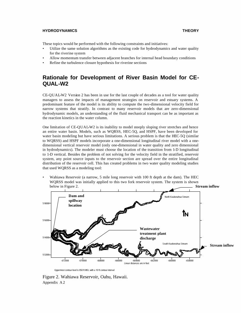
Rationale for Development of River Basin Model for CE-QUAL-W2 CE-QUAL-W2 Version 2 has been in use for the last couple of decades as a tool for water quality managers to assess the impacts of management strategies on reservoir and estuary systems. A predominant feature of the model is its ability to compute the two-dimensional velocity field for narrow systems that stratify. In contrast to many reservoir models that are zero-dimensional hydrodynamic models, an understanding of the fluid mechanical transport can be as important as the reaction kinetics in the water column. One limitation of CE-QUAL-W2 is its inability to model steeply sloping river stretches and hence an entire water basin. Models, such as WQRSS, HEC-5Q, and HSPF, have been developed for water basin modeling but have serious limitations. A serious problem is that the HEC-5Q (similar to WQRSS) and HSPF models incorporate a one-dimensional longitudinal river model with a one-dimensional vertical reservoir model (only one-dimensional in water quality and zero dimensional in hydrodynamics). The modeler must choose the location of the transition from 1-D longitudinal to 1-D vertical. Besides the problem of not solving for the velocity field in the stratified, reservoir system, any point source inputs to the reservoir section are spread over the entire longitudinal distribution of the reservoir cell. This has created problems in two water quality modeling studies that used WQRSS as a modeling tool: • Wahiawa Reservoir (a narrow, 5 mile long reservoir with 100 ft depth at the dam). The HEC

WQRSS model was initially applied to this two fork reservoir system. The system is shown below in Figure 2.

-672000 -670000 -668000 -666000 -664000 -662000 -660000 -658000

512000

514000

516000

518000

North Kaukonahua Stream

South Kaukonahua Stream

Uppermost contour level is 850 ft MSL with a 10 ft contour interval

Linear distances are in feet

Figure 2. Wahiawa Reservoir, Oahu, Hawaii.

Dam and spillway location

Wastewater treatment plant discharge

Stream inflow

Stream inflow

HYDRODYNAMICS

THEORY

Appendix A 3

The WQRSS model schematization is contrasted to the CE-QUAL-W2 schematization for Wahiawa Reservoir in Figure 3. The initial reservoir study using WQRSS produced poor results even after expending large resources to “make” the model work. The modeling effort did not provide a management tool for water quality managers because of gross errors in setting up the model, i.e., combining the 2 forks and spreading the discharge from the wastewater treatment plant throughout the full longitudinal length of the reservoir. • Tualatin River, Oregon (a 32 mile long, narrow, stratified system, with pools 25-30 ft deep).

The WQRSS model was applied to this system incorrectly because the modelers decided to break the system from a river to a reservoir at the location of a wastewater treatment plant discharge. Hence, a large section of the Tualatin that stratified was modeled as completely mixed because the modelers knew it would be inappropriate to spread a point source over 32 miles if this section was chosen as a stratified system. A later application of CE-QUAL-W2 (Berger and Wells, 1995) correctly represented the physics of the system.

In these 2 cases, the application of WQRSS had serious limitations for the reservoir section. CE-QUAL-W2 was subsequently applied to these cases and was able to be used effectively because of its 2-D hydrodynamics and water quality. Other hydraulic and water quality models in common use for unsteady flow include the 1-D dynamic EPA model DYNHYD (Ambrose, et al. 1988), used together with the multidimensional water quality model WASP. WASP relies on DYNHYD for the 1-D hydrodynamics. If WASP is used in a multi-dimensional schematization, the modeler must supply dispersion coefficients to allow transport in the vertical or lateral directions. Also, the Corps model, CE-QUAL-RIV1(Environmental Laboratory, 1995), is a one-dimensional dynamic flow and water quality model used for one-dimensional river or stream sections. Each of these models do not have the ability to characterize adequately the hydraulics or water quality of deeper reservoir systems or deep river pools that stratify. CE-QUAL-W2, even though able to handle narrow systems that stratify, is not well-suited for one-dimensional river channels. In the development of CE-QUAL-W2, vertical accelerations were considered negligible compared to gravity forces. This assumption lead to the approximation of hydrostatic pressure for the z-momentum equation. In sloping channels, this assumption is not always valid because the vertical accelerations cannot be neglected if the x and z axes are aligned with an elevation datum and gravity, respectively. Also, the current CE-QUAL-W2 algorithm does not allow the upstream bed elevation to be above the downstream water surface elevation. If one wanted to use the existing CE-QUAL-W2 for sloping channels, one would have to break the sloping section into multiple small branches. Because water basin modeling is becoming more and more essential for water quality managers, providing the capability for CE-QUAL-W2 to be used as a complete tool for water basin modeling is an essential step in upgrading the state-of-the-art in modeling river basins.

HYDRODYNAMICS

THEORY

Appendix A 4

Inflows from wastewatertreatment plants, North andSouth Fork of K. streams

WQRSS ModelSchematic

CE-QUAL-W2Schematic

South Fork

North Fork N. Fork K. streaminflow

S. Fork K. streaminflow

WTPdischarge

Northforkattachedto southfork

All inflows distributed horizontallyinto each cell, no longitudinal spatialresolution, no distinction betweenNorth and South forks of reservoir,only vertical analysis of water qualityvariability

Both longitudinal andvertical spatialresolution, reservoirnorth and south forkrepresented, as well asisland across from damand cove area on Southfork, laterally averagedcells

Figure 3 Comparison of WQRSS and CE-QUAL-W2 schematization for Wahiawa Reservoir.

HYDRODYNAMICS

THEORY

Appendix A 5

Approach to the Problem There are many approaches that could be implemented within CE-QUAL-W2 for riverine branches. By choosing a theoretical basis for the riverine branches that uses the existing 2-D computational scheme for hydraulics and water quality, the following benefits accrued: • code updates in the computational scheme will affect the entire model rather than just one of

the computational schemes for either the riverine or the reservoir sections leading to easier code maintenance

• no changes would be made to the temperature or water quality solution algorithms • by using the two-dimensional framework, the riverine branches would also have the ability to

predict the velocity and water quality field in two dimensions. This has advantages in modeling the following processes: sediment deposition and scour, particulate (algae, detritus, suspended solids) sedimentation, and sediment flux processes.

• since the entire watershed model has the same theoretical basis, setting up branches and interfacing branches involves the same process whether for reservoir or riverine sections, thus making code maintenance and model set-up easier.

The theoretical approach allowed each branch segment to have a channel slope. The governing equations will then be re-derived assuming that the gravity force in the x and z-momentum equations is adjusted by the channel slope. This is shown schematically in Figure 4.

α

River Section

Reservoir Section

Figure 4. Schematic of river-reservoir linkage where α is the slope of the channel bottom.

g

HYDRODYNAMICS

THEORY

Appendix A 6

Development of Governing Equations for CE-QUAL-W2 This section will formally derive the governing equations for CE-QUAL-W2 highlighting assumptions and limitations of the model equations. Coordinate System The general coordinate system that will be used is shown in Figure 5.

Ω

earth’s rotation

ΩE: rotation rate of earth

earth’s center equatorφ

meridian

xy

z

g

Figure 5. Coordinate system for governing equations (x is oriented E, y is oriented N, and z is oriented upward).

Note that Ω is a vector which represents the angular velocity of the earth spinning on its axis. The rotation of our coordinate system can result in significant horizontal accelerations of fluids. This though is usually restricted to large water bodies, such as large lakes and ocean systems. The force that causes horizontal accelerations as a result of the spinning coordinate system is termed the Coriolis force.

HYDRODYNAMICS

THEORY

Appendix A 7

Turbulent Time-Averaged Equations The governing equations are obtained by performing a mass and a momentum balance of the fluid phase about a control volume. The resulting equations are the continuity (or conservation of fluid mass) and the conservation of momentum equations for a rotating coordinate system (Sabersky et al., 1989; Cushman-Roisin, 1994; Batchelor, 1967). After using the coordinate system in Figure 5, applying the following assumptions: • incompressible fluid • centripetal acceleration is a minor correction to gravity • Boussinesq approximation

1 1 1ρ ρ ρ ρ

ρ ρ ρ ρ

ρ ρο ο

ο=+

≈ = +∆

∆

∆

where where is a base value

and has all variations in

o

and substituting the turbulent time averages of velocity and pressure as defined below • all velocities and pressure are considered the sum of turbulent time averages and deviations

from that average, i.e., u u u= + ′ , where uT

udtt

t T

=+

∫1

as shown in Figure 6. The other

terms are v v v= + ′ ; w w w= + ′ and p p p= + ′ where the overbar represents time

averaged and the prime represents deviation from the temporal average;

u

timet t+T

u

u

Figure 6. Sketch of turburlent time averaging for velocity. the governing equations become after simplification:

Continuity

HYDRODYNAMICS

THEORY

Appendix A 8

∂∂

∂∂

∂∂

ux

vy

wz

+ + = 0

where u, v, w are the velocities in the x, y, and z axes, respectively;

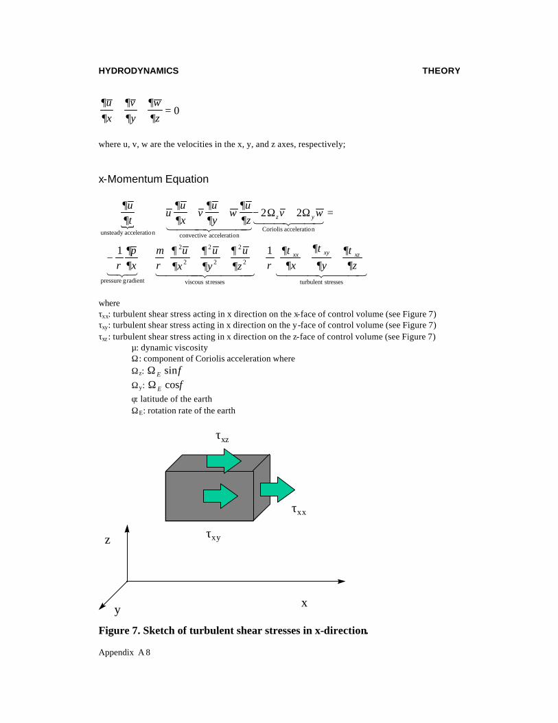
x-Momentum Equation

∂∂

∂∂

∂∂

∂∂

ρ∂∂

µρ

∂∂

∂∂

∂∂ ρ

∂τ∂

∂τ

∂∂τ∂

ut

uux

vuy

wuz

v w

px

ux

uy

uz x y z

z y

xx xy xz

unsteady acceleration convective accelerationCoriolis acceleration

pressure gradient viscous stresses turbulent stresses

+ + + − + =

− + + +

+ + +

1 2444 3444 1 244 344

123 1 24444 34444 1 2444 344

2 2

1 12

2

2

2

2

2

Ω Ω

4

where τxx: turbulent shear stress acting in x direction on the x-face of control volume (see Figure 7) τxy: turbulent shear stress acting in x direction on the y-face of control volume (see Figure 7) τxz : turbulent shear stress acting in x direction on the z-face of control volume (see Figure 7) µ: dynamic viscosity Ω: component of Coriolis acceleration where Ωz: Ω E sinφ

Ωy: Ω E cosφ

φ: latitude of the earth ΩE: rotation rate of the earth

x

z

y

τxz

τxx

τxy

Figure 7. Sketch of turbulent shear stresses in x-direction.

HYDRODYNAMICS

THEORY

Appendix A 9

y-Momentum Equation ∂∂

∂∂

∂∂

∂∂

ρ∂∂

µρ

∂∂

∂∂

∂∂ ρ

∂τ

∂

∂τ

∂

∂τ

∂

vt

uvx

vvy

wvz

u w

py

vx

vy

vz x y z

z x

yx yy yz

+ + + + − =

− + + +

+ + +

2 2

1 12

2

2

2

2

2

Ω Ω

where: τyx: turbulent shear stress acting in y direction on the x-face of control volume (Figure 8) τyy: turbulent shear stress acting in y direction on the y-face of control volume τyz: turbulent shear stress acting in y direction on the z-face of control

Ωx=0

x

z

y

τyz

τyx

τyy

Figure 8. Sketch of turbulent shear stresses in y-direction.

z-Momentum Equation ∂∂

∂∂

∂∂

∂∂

ρ∂∂

µρ

∂∂

∂∂

∂∂ ρ

∂τ∂

∂τ

∂∂τ∂

wt

uwx

vwy

wwz

u v g

pz

wx

wy

wz x y z

y x

zx zy zz

+ + + − + = −

− + + +

+ + +

2 2

1 12

2

2

2

2

2

Ω Ω

where: τzx: turbulent shear stress acting in z direction on the x-face of control volume (Figure 9) τzy: turbulent shear stress acting in z direction on the y-face of control volume τzz: turbulent shear stress acting in z direction on the z-face of control volume

HYDRODYNAMICS

THEORY

Appendix A 10

Ωx=0

x

z

y

τzz

τzx

τzy

Figure 9. Sketch of turbulent shear stresses in z-direction.

Note that the turbulent shear stresses are defined as follows:

τ ρx x u u= ′ ′

τ ρx y u v= ′ ′ is the same as τ ρy x v u= ′ ′

τ ρx z u w= ′ ′ is the same as τ ρzx w u= ′ ′

τ ρy y v v= ′ ′

τ ρy z v w= ′ ′ is the same as τ ρz y w v= ′ ′

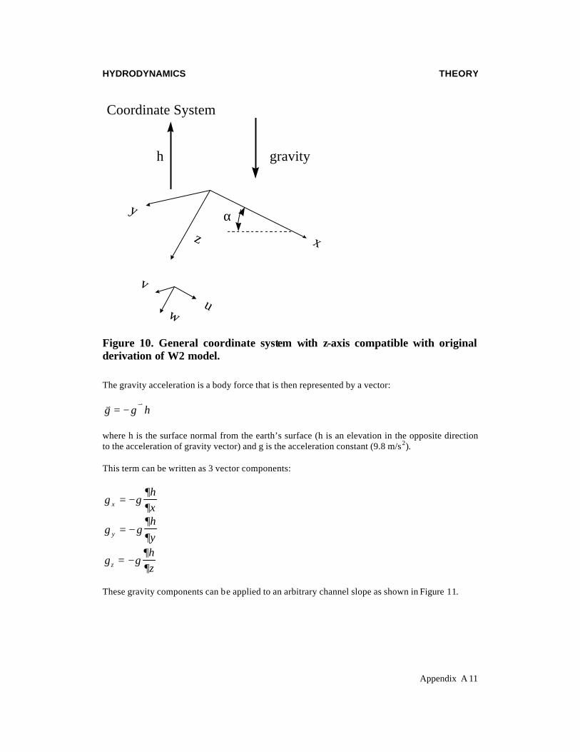
τ ρz z w w= ′ ′ Coriolis Effect As noted above, all the Ωx terms are zero and can be eliminated from the y and z-momentum equations. If one integrates over the y-direction (therefore assuming the net velocity in y is zero) and assumes that the horizontal length scale is much greater than vertical length scale, it can be shown by using scaling arguments that the Coriolis acceleration forces are negligible (Cushman-Roisin, 1994). Hence, prior to lateral averaging, the Coriolis acceleration terms will be neglected. Adjusting the Coordinate System The coordinate system will be transformed into a form compatible with the original W2 development where the vertical axis is in the direction of gravity. Also, as shown in Figure 10, the coordinate system will be oriented along an arbitrary slope.

HYDRODYNAMICS

THEORY

Appendix A 11

z

y

x

Coordinate System

gravity

uw

v

h

α

Figure 10. General coordinate system with z-axis compatible with original derivation of W2 model. The gravity acceleration is a body force that is then represented by a vector: v vg g h= − ∇

where h is the surface normal from the earth’s surface (h is an elevation in the opposite direction to the acceleration of gravity vector) and g is the acceleration constant (9.8 m/s2). This term can be written as 3 vector components:

g ghxx = −

∂∂

g ghyy = −

∂∂

g ghzz = −

∂∂

These gravity components can be applied to an arbitrary channel slope as shown in Figure 11.

HYDRODYNAMICS

THEORY

Appendix A 12

g

h

z x

α

Figure 11. Sketch of channel slope and coordinate system for W2 where the x-axis is oriented along the channel slope. The channel slope can also be incorporated into the definition of the gravity vector if the x-axis is chosen parallel to the channel slope as: The channel slope is defined as So = tanα and also

g ghx

gx = − =∂∂

αsin

g ghz

gz = − =∂∂

αcos

The gravity acceleration in y is assumed to be negligible since ∂∂hy

= 0 in the lateral direction of

the channel. Governing Equations for General Coordinate System After making the following simplifications: • redefine coordinate system • eliminate Coriolis effects

HYDRODYNAMICS

THEORY

Appendix A 13

• neglect viscous shear stresses The governing equations become:

Continuity ∂∂

∂∂

∂∂

ux

vy

wz

+ + = 0

x-Momentum Equation

∂∂

∂∂

∂∂

∂∂

αρ

∂∂ ρ

∂τ∂

∂τ

∂∂τ∂

ut

uux

vuy

wuz

gpx x y z

xx xy xz

unsteady acceleration convective accelerat iongravity

pressure gradient turbulent shear stresses

+ + + = − + + +

1 2444 3444123

123 1 2444 3444sin

1 1

y-Momentum Equation

∂∂

∂∂

∂∂

∂∂ ρ

∂∂ ρ

∂τ

∂

∂τ

∂

∂τ

∂vt

uvx

vvy

wvz

py x y z

yx yy yz+ + + = − + + +

1 1

z-Momentum Equation

∂∂

∂∂

∂∂

∂∂

αρ

∂∂ ρ

∂τ∂

∂τ

∂∂τ∂

wt

uwx

vwy

wwz

gpz x y z

zx zy zz+ + + = − + + +

cos

1 1

Simplification of z-Momentum Equation Assuming that the longitudinal length scale is much greater than the vertical length scale, this makes all vertical velocities << horizontal velocities. A result of this assumption is that vertical velocities are very small such that the z-momentum equation becomes the hydrostatic equation: 1ρ

∂∂

αpz

g= cos

This assumption prevents the model from accurately modeling vertical accelerations of the fluid as a result of convective cooling at night and other such vertical accelerations. Further Simplification of 3-D equations by Lateral Averaging

HYDRODYNAMICS

THEORY

Appendix A 14

The governing equations above will be laterally averaged after decomposing all velocities and pressure into a lateral average and a deviation from the lateral average. The vertical and longitudinal velocities and pressure are defined as follows:

u u u= + " where u u dB y

y= ∫1

1

2y and B is the width of the control volume

w w w= + " v v v= + ′′ p p p= + ′′

The double overbars represent the spatial average of the temporal average quantity. The double prime represents the deviation from the lateral average and is a function of y. This is shown in Figure 12.

x

y

u

y=y1

y=y2

u

u

Figure 12. Lateral average and deviation from lateral average components of longitudinal velocity.

These definitions are substituted into the turbulent time-average governing equations and then laterally averaged. The y-momentum equation is neglected since the average lateral velocities are

zero, i.e., v = 0. , and cross shear stresses that contribute to vertical mixing will be computed from the analysis of wind stress. The equations that remain are the continuity, x-momentum, and z-momentum equations.

HYDRODYNAMICS

THEORY

Appendix A 15

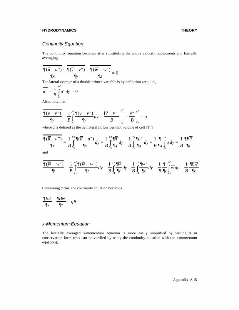
Continuity Equation The continuity equation becomes after substituting the above velocity components and laterally averaging

∂∂

∂∂

∂∂

( ) ( ) ( )u ux

v vy

w wz

+ ′′+

+ ′′+

+ ′′= 0

The lateral average of a double primed variable is by definition zero, i.e.,

′′ = ′′ =∫uB

u dyy

y10

1

2

Also, note that:

( )∂∂

∂∂

( ) ( )v vy B

v vy

dyv v

BvB

qy

y

y

y

y

y+ ′′=

+ ′′=

+ ′′=

′′=∫

1

1

2

1

2

1

2

where q is defined as the net lateral inflow per unit volume of cell [T-1]

∂∂

∂∂

∂∂

∂∂

∂∂

∂∂

( ) ( )u ux B

u ux

dyB

ux

dyB

ux

dyB x

u dyB

Buxy

y

y

y

y

y

y

y+ ′′=

+ ′′= +

′′= =∫ ∫ ∫ ∫

1 1 1 1 1

1

2

1

2

1

2

1

2

and

∂∂

∂∂

∂∂

∂∂

∂∂

∂∂

( ) ( )w wz B

w wz

dyB

wz

dyB

wz

dyB z

w dyB

Bwzy

y

y

y

y

y

y

y+ ′′=

+ ′′= +

′′= =∫ ∫ ∫ ∫

1 1 1 1 1

1

2

1

2

1

2

1

2

Combining terms, the continuity equation becomes

∂∂

∂∂

Bux

Bwz

qB+ =

x-Momentum Equation The laterally averaged x-momentum equation is more easily simplified by writing it in conservation form (this can be verified by using the continuity equation with the x-momentum equation),

HYDRODYNAMICS

THEORY

Appendix A 16

∂∂

∂∂

∂∂

∂∂

αρ

∂∂ ρ

∂τ∂

∂τ

∂∂τ∂

( ) ( )( ) ( )( ) ( )( )

sin( )

u ut

u u u ux

v v u uy

w w u uz

gp p

x x y zxx xy xz

+ ′′+

+ ′′ + ′′+

+ ′′ + ′′+

+ ′′ + ′′=

−+ ′′

+ + +

1 1

Each term in this equation can be simplified as follows (note that the spatial average of any double primed variable goes to zero by definition): • The unsteady acceleration term:

∂∂

∂∂

∂∂

∂∂

∂∂

∂∂

∂∂

( ) ( )u ut B

u ut

dyB

ut

dyB

ut

dyB t

u dyB t

u dyB

Buty

y

y

y

y

y

y

y

y

y+ ′′

=+ ′′

= +′′

= + ′′ =∫ ∫ ∫ ∫ ∫1 1 1 1 1 1

1

2

1

2

1

2

1

2

1

2

• The convective acceleration terms

∂∂

∂∂

∂∂

∂∂

∂∂

∂∂

∂∂

∂∂

∂∂

( )( ) ( )( )u u u ux B

u u u ux

dyB

uux

dyB

u ux

dyB

u ux

dy

B xu udy

B xu u dy

BBuu

x B xu u dy

y

y

y

y

y

y

y

y

y

y

y

y

y

y

dispersion term

+ ′′ + ′′=

+ ′′ + ′′= +

′′+

′′ ′′=

+ ′′ ′′ = + ′′ ′′

∫ ∫∫∫

∫ ∫ ∫

1 1 1 2 1

1 1 1 1

1

2

1

2

1

2

1

2

1

2

1

2

1

2

1 244 344

Similarly for the other 2 terms:

∂∂

∂∂

∂∂

( )( )u u w wz B

Bu wz B z

u w dyy

y

dispersion term

+ ′′ + ′′= + ′′ ′′∫

1 1

1

2

1 244 344

∂∂

( )( )u u v vy

u v u vy y

+ ′′ + ′′= ′′ ′′ − ′′ ′′ =2 1 0

• The gravity term

gB

g dyB

g dy gy

y

y

y

sin sin ( sin ) sinα α α α= = =∫∫1 1

1

2

1

2

• Pressure gradient term

HYDRODYNAMICS

THEORY

Appendix A 17

∂∂

∂∂

∂∂

∂∂

∂∂

∂∂

∂∂

( ) ( )p px B

p px

dyB

px

dyB

px

dyB x

pdyB x

p dyB

Bpxy

y

y

y

y

y

y

y

y

y+ ′′=

+ ′′= +

′′= + ′′ =∫ ∫∫ ∫ ∫

1 1 1 1 1 1

1

2

1

2

1

2

1

2

1

2

or the above equation can be written, assuming that the derivative of the lateral average pressure gradient in the x-direction is not a function of y:

∂∂

∂∂

∂∂

∂∂

∂∂

∂∂

∂∂

( ) ( )p px B

p px

dyB

px

dyB

px

dyB

px

BB x

p dypxy

y

y

y

y

y

y

y+ ′′=

+ ′′= +

′′= + ′′ =∫ ∫∫ ∫

1 1 1 1 1

1

2

1

2

1

2

1

2

• The shear stress terms

∂τ∂

∂τ

∂∂τ∂

∂τ∂

∂τ

∂∂τ∂

∂∂

τ

∂τ

∂∂

τ∂ τ

∂

∂ τ

∂∂ τ

∂∂ τ

∂∂ τ

∂

xx xy xz xx

y

yxy

y

yxz

y

y

xxy

y

xyy

y

xzy

yxx xy xz xx xz

x y z B xdy

B ydy

B zdy

B xdy

B yxdy

B zdy

BB

x

B

yB

z BB

xB

z

+ +

= + + = +

+ = + +

= +

∫ ∫ ∫ ∫

∫ ∫

1 1 1 1

1 1 1 1

1

2

1

2

1

2

1

2

1

2

1

2

Then collecting all terms and neglecting all dispersion terms, the final x-momentum equation is then after simplification:

∂∂

∂∂

∂∂

αρ

∂∂ ρ

∂ τ∂

∂ τ∂

But

Buux

Buwz

BgB p

xB

xB

zxx xz+ + = − + +

sin

1

Summary of Laterally Averaged Equations In the development of CE-QUAL-W2 in Cole and Buchak (1995), the lateral average terms were represented by uppercase characters, such that u U= , w W= , and p P= . The shear stress terms will be assumed to be lateral averages and the double overbars will be dropped for convenience. Making these simplifications, the governing equations become

Continuity Equation ∂∂

∂∂

UBx

+ WB

z = qB

x-Momentum Equation

∂∂

∂∂

∂∂

∂∂

∂∂

∂∂

UBt

+ UUB

x +

WUBz

= sin -Px

+ x

+ B

zx

gBB B xx z

αρ ρ

τρ

τ1 1

HYDRODYNAMICS

THEORY

Appendix A 18

z-Momentum Equation 1ρ

∂∂

αPz

g= cos

Now we have 3 equations and 3 unknowns: U, W, and P.

Simplification of the Pressure Term The z-momentum equation reduces to

P = + ∫P g dza

zcosα ρ

η after integration from a depth z to the water surface defined as z=η. Pa

is the atmospheric pressure at the water surface (see Figure 13).

x

z

z=zsurface=η

z=h=zbottom

gPa

Figure 13. Illustration of layout for simplification of pressure term.

This equation for pressure is now substituted into the x-momentum equation and simplified using Leibnitz rule. The pressure gradient term in the x-momentum equation then becomes:

− = − + − ∫1 1ρ

∂∂ ρ

∂∂

α∂η∂

αρ

∂ρ∂η

Px

Px

gx

gx

dza zcos

cos

HYDRODYNAMICS

THEORY

Appendix A 19

The first term on the RHS is the atmospheric pressure term (accelerations due to atmospheric pressure changes over the water surface), the second is the barotropic pressure term (accelerations due to water surface variations), and the third is the baroclinic pressure term (accelerations due to density driven currents). In CE-QUAL-W2, the atmospheric pressure term is assumed to be zero and is neglected. This implies that for long systems during severe storms the model will not be able to account for accelerations on account of atmospheric changes. (For a large physical domain, variations in meteorological forcing may be significant. This is discussed in Variability in Meteorological Forcing.) The pressure term then becomes with this simplification

− = − ∫1ρ

∂∂

α∂η∂

αρ

∂ρ∂η

Px

gx

gx

dzz

coscos

The revised form of the x-momentum equation is then

∂∂

∂∂

∂∂

+ −∂

∂∂

∂∫

UBt

+ UUB

x +

WUBz

=

sin coscos

+ x

+ B

zxgB g B

xg B

xdz

Bzxx zα α

∂η∂

αρ

∂ρ∂ ρ

τρ

τ

η

1 1

Effectively, we have removed pressure from the unknowns by combining the z-momentum and x-momentum equations, but we have added η as an unknown.

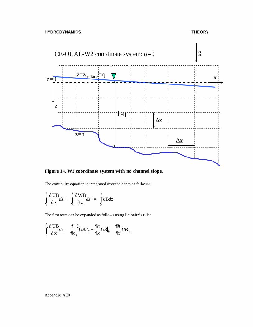
Free Water Surface Equation This equation is a simplification of the continuity equation. The continuity equation integrated over the depth from the water surface to the bottom is called the free water surface equation. Figure 14 and Figure 15 are definition sketches for the CE-QUAL-W2 cell layout without and with a channel slope, respectively.

HYDRODYNAMICS

THEORY

Appendix A 20

x

z

z=zsurface=η

z=h

gCE-QUAL-W2 coordinate system: α=0

z=0

h-η

∆x

∆z

Figure 14. W2 coordinate system with no channel slope.

The continuity equation is integrated over the depth as follows:

∂∂

∂∂∫ ∫ ∫

UBx

+ WB

z = qB

η η η

h h h

dz dz dz

The first term can be expanded as follows using Leibnitz’s rule:

∂∂

= − +∫ ∫UBx

η η

η

∂∂

∂∂

∂η∂

h

h

h

dzx

UBdzhx

UBx

UB

HYDRODYNAMICS

THEORY

Appendix A 21

x

z

z=h

gCE-QUAL-W2 coordinate system: α>0

z=0

h-η

∆z

α

∆x

z=zsurface=η

Figure 15. W2 coordinate system with finite channel slope.

The integral of the vertical flow rate over z relates to changes in water surface elevation as shown below:

WB

z =

∂∂

−∫η

η

h

hdz WB WB

where Wht

Uhxh h= +

∂∂

∂∂

Wt

Uxη η

∂η∂

∂η∂

= +

Combining these term together, the free surface equation becomes

∂∂

∂∂

∂η∂

∂∂

∂∂

∂η∂

∂η∂η

η η η ηηx

UBdzhx

UBx

UB U Bht

U Bhx

Bt

B Ux

qBdzh

h

h h h h

h

− + + + − − =∫ ∫

HYDRODYNAMICS

THEORY

Appendix A 22

Canceling out terms and applying the no-slip boundary condition that Uh is zero,

∂∂

∂η∂η

ηηx

UBdz Bt

qBdzh h

∫ ∫− =

or

Bt x

UBdz qBdzh h

ηη η

∂η∂

∂∂

= −∫ ∫

where Bη is the width at the surface.

Equation of State The density must be know for solution of the momentum equations. The equation of state is an equation that relates density to temperature and concentration of dissolved substances. This equation is termed ρ = f(T , , )w TDS ssΦ Φ

where f(Tw,ΦTDS, Φss)=density function dependent upon temperature, total dis solved solids or salinity, and suspended solids. Hence, the temperature, total dissolved solids, and suspended solids must be known and are determined from the water quality model.

HYDRODYNAMICS

THEORY

Appendix A 23

Summary of Governing Equations Table 1 shows the governing equations after lateral averaging for a channel slope of zero (original model formulation) and for an arbitrary channel slope. Parameters used in Table 1 are illustrated in Figure 16.

Table 1. Comparison of governing equations for CE-QUAL-W2 with and without channel slope. Equation Existing governing equation assuming no channel

slope Governing equation assuming an arbitrary channel slope

x- momentum

∂∂

∂∂

∂∂

−

∂∂

∂∂

∫

UBt

+ UUB

x +

WUBz

=

+

x

+ B

zx

gBx

gBx

dz

B

z

xx z

∂η∂ ρ

∂ρ∂

ρτ

ρτ

η

1 1

∂∂

∂∂

∂∂

+ −

∂∂

∂∂

∫

UBt

+ UUB

x +

WUBz

=

sin coscos

+

x

+ B

zx

gB g Bx

g Bx

dz

B

z

xx z

α α∂η∂

αρ

∂ρ∂

ρτ

ρτ

η

1 1

z-momentum 0

1= −g

Pzρ

∂∂

01

= −gPz

cosαρ

∂∂

free surface equation B

t xUBdz qBdz

h h

ηη η

∂η∂

∂∂

= −∫ ∫ Bt x

UBdz qBdzh h

ηη η

∂η∂

∂∂

= −∫ ∫

Note: U,W: horizontal and vertical velocity B: channel width P: pressure g: acceleration due to gravity τx,τz: lateral average shear stress in x and z ρ: density η: water surface α: channel angle

HYDRODYNAMICS

THEORY

Appendix A 24

α

h

z

xDatum

gravity

channel slope So= = tan α

Figure 16. Definition sketch for channel slope (exaggerated slope).

Linkage of Branches with Internal Head Boundary Conditions Linkage of Mainstem Branches One issue in the development of the river basin model is the linkage of branches of different channel slope orientation. Figure 17 shows in detail some of the variable definitions with the current sloped channel scheme.

HYDRODYNAMICS

THEORY

Appendix A 25

x

z

η

z=h

CE-QUAL-W2 coordinate system

z=0

∆xi

Ηk=∆zk

kt

kt+1

i-1 i i+1

kb

Segment

Layer

k

k-1

k+1

ρ,Φ,P,BU,Ax,Dx,BR, τxx

W,BB,DzAz

α

Figure 17. Variable definitions for W2 model with arbitrary channel slope.

But the vertical velocity of a cell is not determined at the side edge of a segment, but at the bottom of the segment. In order for all the volume to be passed from one cell to another, all the flow from the downstream segment (ID) should be transferred to upstream segment (IU). Since the model does not assume strong vertical accelerations, we may be forced to neglect the vertical component of velocity at this transition and assume that the longitudinal velocity entering segment IU is UID. The linkage between branches when the grid sizes are different between the upstream grid and the downstream grid were accomplished by flow and mass conservation at the linkage. This is computed internally. This spatial averaging of the flow (and velocity), heat and mass to preserve flow and constituent mass between branches is illustrated conceptually in Figure 18.

HYDRODYNAMICS

THEORY

Appendix A 26

ID

IU

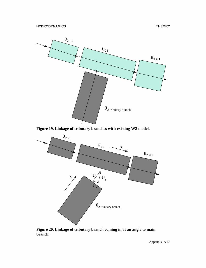
Figure 18. Transfer of mass and momentum between main stem branches with unequal grid spacing. Linkage of Tributary Branches The existing W2 model assumes all tributary branches come in at right angles to the main channel. In many cases this is appropriate. This orientation (shown in Figure 19) allows volume exchange, but no momentum exchange between branches. The CE-QUAL-RIV1 model (Environmental Laboratory, 1995) and the EPA DYNHYD (Ambrose, et al., 1988) als o neglect momentum effects of lateral tributary inflows. For branches with arbitrary channel orientation (as in Figure 20), code changes will be made to allow momentum, in addition to volume (this is accounted for in the free surface equation as q), to be exchanged between branches. In this section the linking of these tributary branches with the main stem and preserving momentum between them will be discussed.

HYDRODYNAMICS

THEORY

Appendix A 27

θ2 i-1

θ2 i+1

θ2 i

θ2 tributary branch

Figure 19. Linkage of tributary branches with existing W2 model.

θ2 i-1

θ2 i+1

θ2 i

θ2 tributary branch

x

x U Uy

Ux

Figure 20. Linkage of tributary branch coming in at an angle to main branch.

HYDRODYNAMICS

THEORY

Appendix A 28

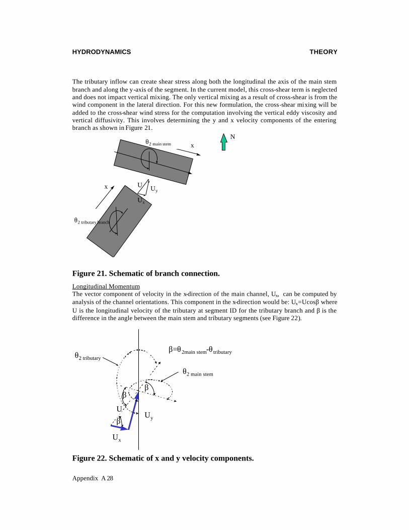
The tributary inflow can create shear stress along both the longitudinal the axis of the main stem branch and along the y-axis of the segment. In the current model, this cross-shear term is neglected and does not impact vertical mixing. The only vertical mixing as a result of cross-shear is from the wind component in the lateral direction. For this new formulation, the cross-shear mixing will be added to the cross-shear wind stress for the computation involving the vertical eddy viscosity and vertical diffusivity. This involves determining the y and x velocity components of the entering branch as shown in Figure 21.

θ2 main stem

θ2 tributary branch

x

x U Uy

Ux

N

Figure 21. Schematic of branch connection.

Longitudinal Momentum The vector component of velocity in the x-direction of the main channel, Ux, can be computed by analysis of the channel orientations. This component in the x-direction would be: Ux=Ucosβ where U is the longitudinal velocity of the tributary at segment ID for the tributary branch and β is the difference in the angle between the main stem and tributary segments (see Figure 22).

Ux

Uy

β

θ2 main stem

θ2 tributaryβ=θ2main stem-θtributary

β

β

U

Figure 22. Schematic of x and y velocity components.

HYDRODYNAMICS

THEORY

Appendix A 29

The conservation of momentum about a control volume, the main stem segment, would result in an additional source of momentum. Lai (1986) shows that the correction to the x-momentum equation would be: qBU x where q is the lateral inflow per unit length. This arises from re-deriving the momentum equations and assuming that all the fluid (q) entering the segment is moving at the velocity Ux. This correction to the x-mo mentum equation would be

∂∂

∂∂

∂∂

+ −

∂∂

∂∂

+

∫UB

t +

UUBx

+ WUB

z = sin cos

cos +

x

+ B

zx

gB g Bx

g Bx

dz

BqBU

z

xx zx

α α∂η∂

αρ

∂ρ∂

ρτ

ρτ

η

1 1

momentum from side tributaries123

Cross-shear of Tributary Inflow The y-velocity coming into a reservoir also may contribute significantly to vertical mixing. The y component of a tributary inflow is (see Figure 34): Uy=Usinβ. Since there is no y-momentum equation, the only mechanism for mixing energy with the present formulation of the vertical shear

stress is the cross-shear stress from the wind given earlier as τ ρwy D a hC W≅ −21 2sin( )Θ Θ .

This cross-shear stress accounts for the shear stress and mixing that results from wind blowing across the y-axis of the segment. The lateral branch inflow at a velocity, Uy, could be thought of as an additional component of that stress under the current context of the turbulence closure approximations. Assuming that the water in the y-direction has zero velocity, the additional shear stress could be parameterized as an interfacial shear:

τ ρytributary y

fU≅

82

where f is an interfacial friction factor. For two-layer flow systems, f has been found to be of order 0.01. The value of f for this non-ideal approach could be determined by numerical computation. Hence, the value of the cross-shear term would be increased by a lateral tributary inflow. This will be evaluated by numerical experiments computing the magnitude of the cross-shear term from wind and from lateral inflow. A more robust theoretical approach may be needed to account for this increase in lateral shear, but that may be necessary only if the model includes the y-momentum equation.

HYDRODYNAMICS

THEORY

Appendix A 30

Implementation of River Basin Model in W2 Solution Technique The corrections to the governing equations incorporating the sloping channel and the transfer of momentum from a side tributary are incorporated in the new solution technique as shown below. Numerical Solution for the Free-Water Surface Equation The following derivation of the solution technique will follow the derivation format and approach used in Cole and Buchak (1995). Deviations from or minor corrections from that approach will be noted. The free surface equation,

Bt x

UBdz qBdzh h

ηη η

∂η∂

∂∂

= −∫ ∫

will be solved by substituting the momentum equation,

∂∂

∂∂

∂∂

+ −

∂∂

∂∂

+

∫UB

t +

UUBx

+ WUB

z = sin cos

cos +

x

+ B

zx

gB g Bx

g Bx

dz

BqBU

z

xx zx

α α∂η∂

αρ

∂ρ∂

ρτ

ρτ

η

1 1

in finite difference form and then simplifying. The finite difference form of the momentum equation is

UB UB t gB g Bx

g Bx

dz

BqBU

in

in

z

xx zx i

n

+ = + −∂

∂−

∂∂

+ + −

∂∂

∂∂

+

∫1

1 1

UUB

x

WUBz

sin coscos

+

x

+ B

zx

∆ α α∂η∂

αρ

∂ρ∂

ρτ

ρτ

η

Defining for simplicity the term F as

FB xx= −

∂∂

−∂

∂+

∂∂

UUB

x

WUBz

x

1ρ

τ

or substituting in for τxx, F becomes

HYDRODYNAMICS

THEORY

Appendix A 31

FBA

Uxx

= −∂

∂−

∂∂

+∂

∂

UUBx

WUB

z

x

∂∂

(Note that in Cole and Buchak (1995) the term F is defined differently in Equation A-10 than in

Equation A-18.) Substituting in the term UBin+1 in the free surface equation for UB, the free

surface equation becomes

∫∫∫∫∫

∫∫∫∫

−∆+∂

∂∆∆

−∆+∆+∆+=

hnn

x

hnz

hz nh

nhhhnn

i

h

BdzqdzqBUx

tdzx

tdzdzx

Bgx

t

dzx

Bgx

tdzgBx

tdzFx

tdzUBxt

B

ηηηηη

ηηηηη

∂∂τ

ρ∂∂

∂∂ρ

ρα

∂∂

∂∂η

α∂∂

α∂∂

∂∂

∂∂

∂∂η

zB1 + cos

cossin

x

Some of these terms can be simplified as follows:

∂∂

α α∂∂η ηx

gB dz gx

Bdzh h

∫ ∫=sin sin

∂∂

α∂η∂

α∂∂

∂η∂η ηx

g Bx

dz gx x

Bdzh h

∫ ∫=

cos cos

∂∂

αρ

∂ρ∂

αρ

∂∂

∂ρ∂η η η ηx

g Bx

dzdzg

xB

xdzdz

h z h z

∫ ∫ ∫ ∫=cos

cos

( )∂∂ ρ

τρ

∂∂

τ τη

ηxdz

x

hz

z h z∫∂

∂= −

Bz

B Bxx x

1 1

Then substituting these into the above equation we obtain

( ) ∫∫∫∫

∫∫∫∫

−∆+−∆∆

−

∆+∆+∆+=

hnn

x

hn

zhz

z nh

hnhhnn

i

h

BdzqdzqBUx

tx

tdzdzx

Bx

gt

Bdzxx

tgBdzx

tgdzFx

tdzUBxt

B

ηηη

ηη

ηηηηη

∂∂

ττρ∂

∂∂∂ρ

∂∂

ρα

∂∂η

∂∂

α∂∂

α∂∂

∂∂

∂∂η

xx BB1

+ cos

cossin

Then all terms with η are grouped on the LHS such that

HYDRODYNAMICS

THEORY

Appendix A 32

( ) ∫∫∫∫

∫∫∫∫

−∆+−∆∆

−∆+∆+=

∆−

hnn

x

hn

zhz

z nh

hhnn

i

hh

BdzqdzqBUx

tx

tdzdzx

Bx

gt

Bdzx

tgdzFx

tdzUBx

Bdzxx

tgt

B

ηηη

ηη

ηηηηη

∂∂

ττρ∂

∂∂∂ρ

∂∂

ρα

∂∂

α∂∂

∂∂

∂∂η

∂∂

α∂∂η

xx BB1

+ cos

sin cos

The first term on the LHS can be put into a backward finite difference form as

tB

tB

ni

ni

∆−

≈−1ηη

∂∂η

ηη

The second term

nh

Bdzxx

tg

∆− ∫

η∂∂η

∂∂

αcos , can be simplified using the chain rule for

partial differential equations as nhhn

xBdztgBdz

xxtg

2

2

coscos∂

η∂α

∂∂

∂∂η

αηη∫∫ ∆−∆−

Then using a second order central difference for the second derivative and a first order backward difference for the first derivative such that

2111

2

2

2coscos

coscos

xBdztgBdz

xxtg

xBdztgBdz

xxtg

ni

ni

ni

hhni

ni

nhhn

∆+−

∆−∆−

∆−

≈∆−∆−

−+− ∫∫

∫∫ηηη

α∂∂ηη

α

∂η∂

α∂∂

∂∂η

α

ηη

ηη

Also, noting using a backward difference

n

i

h

i

hh

BdzBdzx

Bdzx

−

∆=

−

∫∫∫1

1

ηηη∂∂

.

Then grouping and collecting terms and multiplying through by ∆t∆x, the LHS becomes after simplification

HYDRODYNAMICS

THEORY

Appendix A 33

xBtxRHSBdzx

tg

BdzBdzx

tgxBBdz

xtg

ni

ni

i

hni

i

h

i

hni

i

hni

∆+∆∆=

∆∆−

+

+∆

∆+∆+

∆∆−

−+

−−

−

∫

∫∫∫

12

1

1

2

1

2

1

)(cos

coscos

ηα

η

αη

αη

ηη

ηηη

η

where the RHS is defined as

( ) ∫∫∫∫

∫∫∫

−∆+−∆∆

−∆+∆+=

h

x

h

zhz

zh

hhni

h

qBdzdzqBUx

tx

tdzdzx

Bx

gt

Bdzx

tgdzFx

tdzUBx

RHS

ηηη

ηη

ηηη

∂∂

ττρ∂

∂∂∂ρ

∂∂

ρα

∂∂

α∂∂

∂∂

xx BB1

+ cos

sin

and is evaluated at time level n. The integral of the cell widths can be put into a summation over the vertical layers as

Bdz BHh

i

rikb

kt

η∫ ∑=

Bdz BHh

i

rikb

kt

η∫ ∑

−

−=1

1

where BHr is the value of the width times the layer depth for the right-hand side of a cell (see Figure 23). In the W2 code this is the variable BR(I,K) times H(K), or the derived variable BHR(I,K).

HYDRODYNAMICS

THEORY

Appendix A 34

x

z

η

z=h

z=0

∆xi

Ηk=∆zk

i-1 i i+1

k

k-1

k+1

ρ,Φ,P,BU,Ax,Dx,BR, τxx

W,BB,DzAz

α

U(I,K)U(I-1,K)

W(I,K)

W(I,K-1)

Figure 23. Cell grid definitions. Some of the RHS terms can be put into a format compatible with the model schematization such as

( ) ( )nkb

ktirir

i

kb

ktr

i

kb

ktr

kb

ktr

ni

h

UBHUBHx

UBHUBHx

UBHx

dzUBx ∑∑∑∑∫ −

−

−∆

=

−

∆≈≈

11

11∂∂

∂∂

η

( )nkb

ktirir

i

kb

ktr

i

kb

ktr

kb

ktr

hn FHFH

xt

FHFHxt

FHx

tdzFx

t ∑∑∑∑∫ −−

−∆∆

=

−

∆∆

≈∆≈∆1

1

∂∂

∂∂

η

∆ ∆∆

∆

∆∆

tgx

Bdz tgx

BHtg

xBH BH

tgx

BH BH

h

rkt

kb

rkt

kb

ir

kt

kb

i

r ikt

kb

r i

sin sinsin

sin( )

α∂∂

α∂∂

α

αη∫ ∑ ∑ ∑

∑

≈ ≈ −

=

−

−

−

1

1

HYDRODYNAMICS

THEORY

Appendix A 35

( )

∆ ∆

∆∆

tg

xB

xdzdz t

gx

Bx

H dz

tg

x xH BH BH

h z h

rkt

kb

rkt

kb

r i r ikt

kb

cos cos

cos

αρ

∂∂

∂ρ∂

αρ

∂∂

∂ρ∂

αρ

∂ρ∂

η η η∫ ∫ ∫ ∑

∑ ∑

≈ ≈

−−1

( ) ( ) ( ) ∆∆∆

tx

txz h z z h z

iz h z

i

∂∂ ρ

τ τρ

τ τ τ τη η η

11

B B B B B Bx x x x x x− ≈ − − −−

The lateral inflow of momentum term represents the gradient over x of the inflow momentum.

∑∫ ∆≈∆kb

ktrxx

h

BHqUx

tdzqBUx

t∂∂

∂∂

η

qBdz qBHh

rkt

kb

η∫ ∑≈

Compiling these terms into one equation, we obtain

DCXA ni

ni

ni =++ +− 11 ηηη

where

Ag t

xBHr

kt

kb

i

=−

∑

−

cosα∆∆

2

1

+∆

∆+∆=

−∑∑

1

2cos

i

kb

ktr

i

kb

ktr BHBH

xtg

xBXα

η

Cg t

xBHr

kt

kb

i

=−

∑cosα∆

∆

2

( ) ( )

( ) ( )

( ) ( )[ ]1

22

12

12

121

1

cossin

−

−−

−−

−

−−−∆

+∂∂

∆∆+∆∆

+−∆+−∆

+−∆+∆+−∆=

∑∑

∑ ∑∑

∑∑

ixzhxzixzhxz

kb

ktrx

kb

ktr

kb

kt

kb

ktririr

kb

ktirir

kb

ktirir

ni

kb

ktirir

BBBBt

BHqUx

txqBHtx

Hx

BHBHg

tBHBHgt

FHFHtxBUBHUBHtD

ηη

η

ττττρ

∂∂ρ

ρα

α

η

HYDRODYNAMICS

THEORY

Appendix A 36

This equation is solved for the water surface elevation at the n+1 time level using the Thomas algorithm. The boundary condition implementation is the same as described in Cole and Buchak (1995). Numerical Solution of the Horizontal Momentum Equation The x-momentum equation,

xzxx

z

qBUB

dzx

Bgx

BggB

+∂

∂∂

∂

−+∂

∂∂

∂∂

∂∫

zB1

+ x

1

+ coscossin = z

WUB + x

UUB + t

UB

xτρ

τρ

∂∂ρ

ρα

∂∂ηαα

η

is solved using either a fully explicit or an explicit/implicit finite difference solution technique. In the W2 Version 3 code, the User specifies either of these techniques.

Explicit Solution This scheme is based on solving the partial differential terms using an explicit finite difference technique where

nix

zxx

zni

ni

ni

ni

qBUB

dzx

Bgx

BggBtBUBU

z

B1 +

x1

+ cos

cossin z

WUB

xUUB

x

11

+∂

∂∂

∂

−++∂

∂−

∂∂

−∆+= ∫++

τρ

τρ

∂∂ρ

ρα

∂∂η

ααη

The various terms are put into finite difference form as follows: This longitudinal advection of momentum [termed ADMX in the W2 code] is an upwind difference scheme (where the order of differencing is dependent on the sign of U), i.e., for U>0

[ ]nki

nki

nki

nki

nki

nki

iki

UUBUUBx ,1,2/1,1,,2/1,

,

1x

UUB−−−+ −

∆≅

∂∂

The vertical advection of momentum [termed ADMZ in the W2 code] is also an upwind scheme based on the velocity of W, i.e., for W>0 or downward flow

( ) ( )[ ]nki

nki

nki

nki

nki

nki

kki

BUWBUWz 1,1,1,,,,

,

1z

WUB−−−−

∆≅

∂∂

The gravity force [termed GRAV in the W2 code] is

HYDRODYNAMICS

THEORY

Appendix A 37

niBggB αα sinsin =

The pressure gradient [termed HPG in the W2 code] is

( ) ( ) kn

kiki

nin

ii

ni

z

zxBg

xBg

dzx

Bgx

Bg ∆−∆

−−∆

=− ++∫ ,,11coscoscos

cos ρρρ

αηη

α∂∂ρ

ρα

∂∂η

αη

The horizontal advection of turbulent momentum [termed DM in the W2 code] is

( ) ( )nki

nki

ii

xnin

kin

kiii

xni

xxx UU

xxAB

UUxx

ABxU

BAB,1,

2/1

2/1,,1

2/1

2/1

x

x1

−−

−+

+

+ −

∆∆

−−

∆∆

=∂

∂∂

∂=

∂∂ τ

ρ

The contribution to longitudinal momentum by lateral branch inflows is

n

kixx qBUqBU,

=

Using the definition of the shear stress,

∂∂

++=zU

Aztionbottomfricwindz τττ x ,

the vertical transport of momentum is

( )

( )

−

∆++

∆∆

−

−

∆++

∆∆=

∂∂

++∂∂

=∂

∂

−−

−

−−

−

−

++

+

++

+

+

nki

nki

k

kizn

kitionbottomfricn

kiwind

kk

nki

nki

nki

k

kizn

kitionbottomfricn

kiwind

kk

nki

ztionbottomfricwindz

UUz

A

zzB

UUz

A

zzB

zU

AB

1,,2/1

2/1,

2/1,2/1,

2/1

2/1,

,1,2/1

2/1,

2/1,2/1,

2/1

2/1,x

zzB1

ττ

ρ

ττ

ρττ

ρτ

ρ

Implicit Scheme The implicit technique was utilized to reduce the time step limitation for numerical stability when values of Az were large, as for an estuary or a river system. This occurs because the time step limitation is a function of Az. Only the vertical transport of momentum term was solved

HYDRODYNAMICS

THEORY

Appendix A 38

implicitly. All other terms for the solution of the horizontal momentum equation were the same as the explicit scheme. The horizontal momentum equation was split into the following 2 equations:

xwindtionbottomfricxx

z

qBUB

dzx

Bgx

BggB

+∂

+∂

∂∂

−+∂

∂∂

∂∂

∂∫

z

)B(1 +

x1

+ cos

cossin = z

WUB +

xUUB

+ t

UB

ττ

ρτ

ρ

∂∂ρ

ρα

∂∂η

ααη

( 1) and

∂∂

∂∂

=∂

∂zU

BAzt

UBzρ

1

(2) Equation 1 is written as

( ) nix

windtionbottomfricxx

zni

ni

nii

qBUB

dzx

Bgx

BggBtBUBU

z

B1 +

x1

+ cos

cossin z

WUB

xUUB

1*

+∂

+∂

∂∂

−++∂

∂−

∂∂

−∆+= ∫+

ττ

ρτ

ρ

∂∂ρ

ρα

∂∂η

ααη

(3) where U* is the velocity at the new time level before the application of Equation 2. Equation 3 is solved similarly to the solution of the fully explicit technique outlined above. Equation 2 is then solved using a fully implicit technique as

( )

∂

∂∂∂

=∆−

=∂

∂ ++

+++

zU

ABzt

BUBUt

UB n

zn

nii

ni

ni

11

1*11 1ρ

This can be rewritten as

( )

( )

−

∆

∆∆

−

−

∆

∆∆

+=

+−

+

−

−

+−++

++

++

++++

11,

1,

2/1

2/1,

12/1,1

,1

1,2/1

2/1,1

2/1,1*11

nki

nki

k

kiz

k

nkin

kinki

k

kiz

k

nkin

iini

ni

UUz

A

ztB

UUz

A

ztB

BUBUρρ

Regrouping terms at n+1 time level on the LHS, the equation can be written as

HYDRODYNAMICS

THEORY

Appendix A 39

*,

11,

1,

11, ki

nki

nki

nki DUCUVUAU =++ +

+++

−

where

∆

∆∆−

=−

−+

+−

2/1

2/1,1

,

12/1,

k

kiz

kn

ki

nki

zA

zBtB

Aρ

∆

∆∆

+

∆

∆∆

+=−

−+

+−

+

++

++

2/1

2/1,1

,

12/1,

2/1

2/1,1

,

12/1,1

k

kiz

knki

nki

k

kiz

knki

nki

zA

zBtB

zA

zBtB

Vρρ

∆

∆∆−

=+

++

++

2/1

2/1,1

,

12/1,

k

kiz

knki

nki

zA

zBtB

Cρ

1=D The resulting simultaneous equations are solved for Un+1 using the Thomas algorithm.

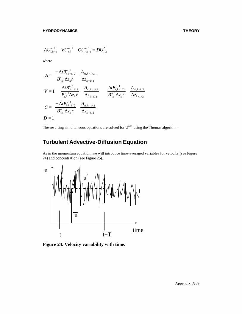
Turbulent Advective-Diffusion Equation As in the momentum equation, we will introduce time-averaged variables for velocity (see Figure 24) and concentration (see Figure 25).

u

timet t+T

u

u

Figure 24. Velocity variability with time.

HYDRODYNAMICS

THEORY

Appendix A 40

c

timet t+T

c

c

Figure 25. Variability of concentration with time. Here we take the instantaneous velocity and concentration and decompose it into a mean and an unsteady component, as

u(t) = u + u (t) where u = 1T

u(t)dttt + T′ ∫

Similarly for w, v, and c:

v = v + v

w = w + w

c = c + c

′

′

′

Then substituting these into the 3-D governing equation and time averaging the equation, we obtain:

( ) ( ) ( )

∂∂

∂∂

∂∂

∂∂

∂∂

∂∂

∂∂

∂∂

′ ′∂

∂′ ′

∂∂

′ ′

ct

+ ucx

+ vcy

+ wcz

= D c

x +

cy

+ c

z

- x

u c - y

v c - z

w c

transport by mean advection

2

2

2

2

2

2

molecular diffusive transport

turbulent mass tranport

1 24444 34444 1 24444 34444

1 24444444 34444444 + r

The “new terms” in our governing equation represent mass transport by turbulent eddies. As the intensity of turbulence increases, turbulent mass transport increases. Notice also that all velocities and concentrations are time averaged. We now define the following turbulent mass fluxes:

HYDRODYNAMICS

THEORY

Appendix A 41

( )

( )

( )

( )

Turbulent mass flux: J = u c , v c , w c

and,

u c = - E cx

v c = - E cy

w c = - E cz

t

x

y

z

′ ′ ′ ′ ′ ′

′ ′∂∂

′ ′∂∂

′ ′∂∂

where Ex, Ey, and Ez are turbulent diffusion coefficients. Substituting into the above equation:

( )

( ) ( ) r + zc

D + E z

+ yc

D + E y

+

xc

D + E x

= zc

w + yc

v + xc

u + tc

zy

x

∂∂

∂∂

∂∂

∂∂

∂∂

∂∂

∂∂

∂∂

∂∂

∂∂

In turbulent fluids, Ex, Ey, and Ez >> D, hence D can be neglected, except at interfaces where turbulence goes to zero. The turbulent diffusion coefficients can be thought of as the product of the velocity scale of turbulence and the length scale of that turbulence. These coefficients are related to the turbulent eddy viscosity - one is turbulent mass transport , the other is turbulent momentum transport between adjacent control volumes. In general, these turbulent diffusion coefficients are non-isotropic and non-homogeneous.

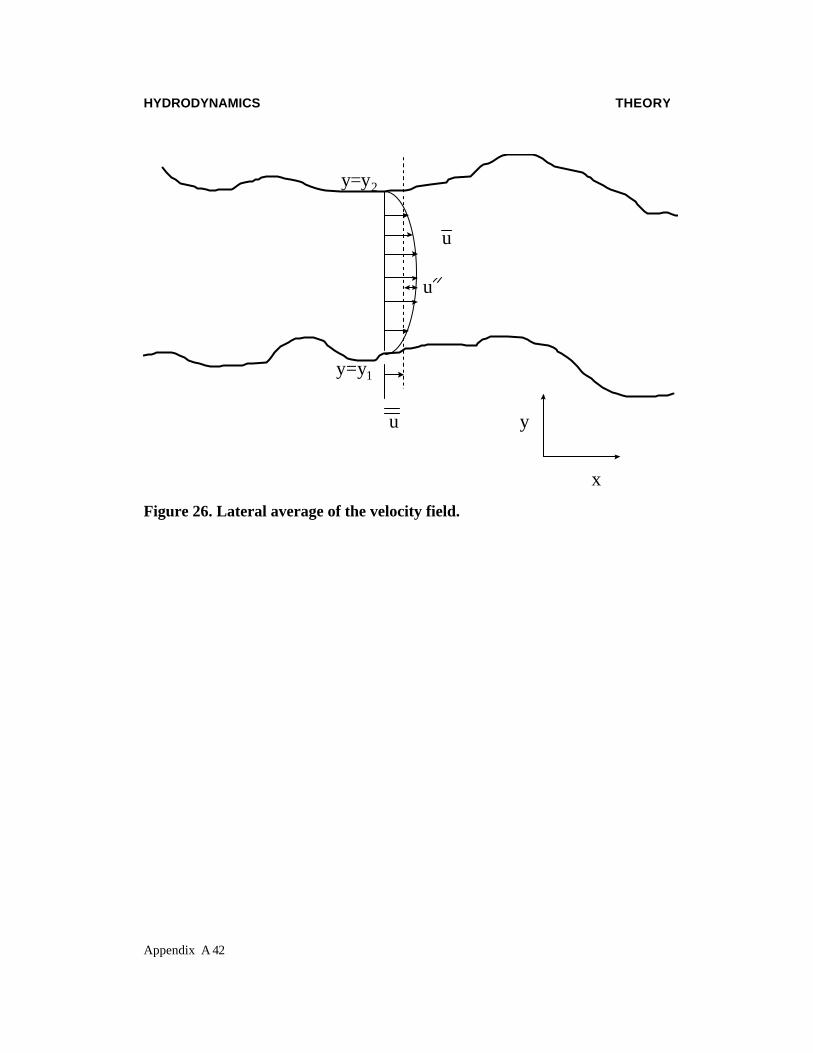
Development of W2 Water Quality Transport Model For a 2-D model like CE-QUAL-W2, we will now introduce spatial averages across the lateral dimension of the channel of the turbulent time -averaged quantities, such as

c = c + c"

u = u + u"

w = w + w"

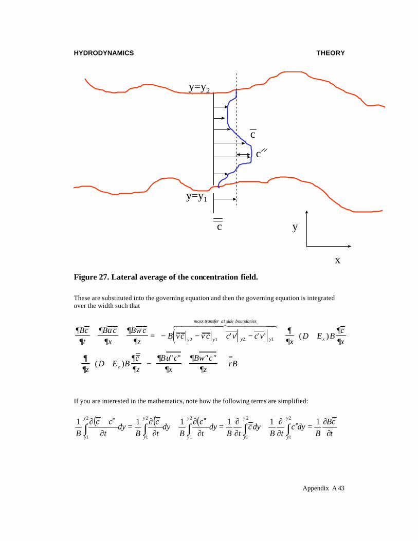
where the double overbar is a spatial average over y and the double prime is the deviation from the spatial mean as illustrated in Figure 26 for velocity and Figure 27).

HYDRODYNAMICS

THEORY

Appendix A 42

x

y

u

y=y1

y=y2

u

u

Figure 26. Lateral average of the velocity field.

HYDRODYNAMICS

THEORY

Appendix A 43

x

y

c

y=y1

y=y2

c

c

Figure 27. Lateral average of the concentration field. These are substituted into the governing equation and then the governing equation is integrated over the width such that

( )∂∂

∂∂

∂∂

∂∂

∂∂

∂∂

∂∂

∂∂

∂∂

Bct

Bucx

Bw cz

B vc v c c v c vx

D E Bcx

zD E B

cz

Bu cx

Bw cz

rB

y y y y

mass transfer at side boundaries

x

z

+ + = − − + − + +

+

+ +

− +

′′ ′′

+

2 1 2 1' ' ' ' ( )

( )" "

6 7444444 8444444

If you are interested in the mathematics, note how the following terms are simplified:

( ) ( ) ( )tcB

Bdyc

tBdyc

tBdy

tc

Bdy

tc

Bdy

tcc

B

y

y

y

y

y

y

y

y

y

y ∂∂

=′′∂∂

+∂∂

=∂

′′∂+

∂∂

=∂

′′+∂∫∫∫∫∫

111111 2

1

2

1

2

1

2

1

2

1

HYDRODYNAMICS

THEORY

Appendix A 44

( )( ) ( ) ( )

xcuB

BtcuB

B

dyucxB

dyucxB

dytuc

Bdy

tuc

Bdy

xccuu

B

y

y

y

y

y

y

y

y

y

y

∂′′′′∂

+∂

∂

=′′′′∂∂

+∂∂

=∂

′′′′∂+

∂∂

=∂

′′+′′+∂∫∫∫∫∫

11

11111 2

1

2

1

2

1

2

1

2

1

Note that the spatial average of any double primed variable goes to zero by definition. These turbulent dispersion coefficients are defined as

w c Dcz

u c Dcx

z

x

" "

" "

= −

= −

∂∂

∂∂

These dispersion terms are a result of spatial averaging of the velocity field laterally. In general, except at an interface, Dx >> Ex >> D and similarly for Dz >> Ez >> D. Substituting in for the dispersion coefficients, and using q to be the net mass transport from lateral boundaries, this equation becomes

Brzc

BDzx

cBD

xqB

zcwB

xcuB

tcB

zx +

+

+=++

∂∂

∂∂

∂∂

∂∂

∂∂

∂∂

∂∂

If we drop the overbars replacing them with capitals, replace c with Φ, we then obtain the governing equation of CE-QUAL-W2:

∂∂

∂∂

∂∂

∂∂Φ∂

∂

∂∂Φ∂

∂B

t +

UBx

+ WB

z -

BDx

x -

BDz

z = q B + S B

x zΦ Φ ΦΦ Φ

Φ = laterally averaged constituent concentration, g m-3 Note that this can be concentration or temperature since the concentration of heat can be

determined to be ρcpT where ρ is the fluid density, cp is the specific heat of water, and T is the temperature. Hence, the above equation with C or ρcpT for Φ would be appropriate governing equations for concentration or temperature, respectively.

Dx = longitudinal temperature and constituent dispersion coefficient, m2 sec-1 Dz = vertical temperature and constituent dispersion coefficient, m2 sec-1 qΦ = lateral inflow or outflow mass flow rate of constituent per unit

volume,

HYDRODYNAMICS

THEORY

Appendix A 45

g m-3 sec-1 SΦ = laterally averaged source/sink term, g m-3 sec-1 In order to solve this equation we now need to determine the following: • laterally averaged velocity field - from momentum equations • appropriate boundary and initial conditions • Dx and Dz • source/sink terms laterally averaged

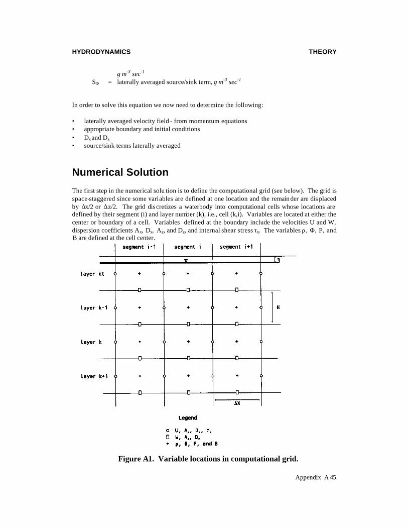
Numerical Solution The first step in the numerical solu tion is to define the computational grid (see below). The grid is space-staggered since some variables are defined at one location and the remain der are dis placed by ∆x/2 or ∆z/2. The grid dis cretizes a waterbody into computational cells whose locations are defined by their segment (i) and layer number (k), i.e., cell (k,i). Variables are located at either the center or boundary of a cell. Variables defined at the boundary include the velocities U and W, dispersion coefficients Ax, Dx, Az, and Dz, and internal shear stress τx. The variables ρ, Φ, P, and B are defined at the cell center.

Figure A1. Variable locations in computational grid.

HYDRODYNAMICS

NUMERICAL SOLUTION

Appendix A 46

There is a rational basis for choosing variable locations. Since the constituent concentration is defined at the center and velocities are defined at the boundaries, spatial averaging of velocities is not required to determine changes in concentration over time. Also, the horizontal velocity is surrounded by a cell with water surface elevations and densities defined on either side. Thus, the horizontal velocity is computed from horizontal gradients of the surface slope and densities without requiring spatial averaging of these variables. The geometry is specified in Figure 1 by a cell width B, cell thickness H, and cell length ∆x. Several additional geometric variables are used in the calculations. These include the average cross-sectional area between two cells (k,i) and (k,i+1)

the average widths between two cells (k,i) and (k+1,i)

and the average layer thickness between layers k and k+1

The numerical procedure for solving the six unknowns at each timestep is to first compute water surface elevations from equation (A-13). With the new surface elevations, new horizontal velocities can be computed from equation (A-9). With new horizontal velocities, the vertical velocities can be found from continuity, equation (A-5). New constituent concentrations are computed from the constituent balance, equation (A-1). Using new horizontal and vertical velocities, the water surface elevation equation, equation (A-13), can be solved for η simultaneously. The solution for η is thus spatially implicit at the same time level and eliminates the surface gravity wave speed criterion:

which can seriously limit timesteps in deep waterbodies. Constituent Transport Version 1.0 used upwind differencing in the constituent transport advective terms in which the cell concentration immediately upstream of the velocity is used to calculate fluxes. A major problem with upwind differencing is the introduction of numerical diffusion given by (for longitudinal advection):

k,irk,i k,i k ,i k ,i+1B H = B H + B H

2 (A-14)

k,ibk,i k+1,iB = B + B

2 (A-15)

k,ik k+1

H = H + H2

(A-16)

∆∆

t < x

g Hmax

(A-17)

HYDRODYNAMICS

NUMERICAL SOLUTION

Appendix A 47

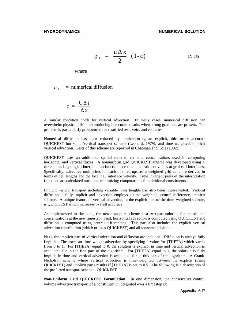
A similar condition holds for vertical advection. In many cases, numerical diffusion can overwhelm physical diffusion producing inaccurate results when strong gradients are present. The problem is particularly pronounced for stratified reservoirs and estuaries. Numerical diffusion has been reduced by imple menting an explicit, third-order accurate QUICKEST horizontal/vertical transport scheme (Leonard, 1979), and time-weighted, implicit vertical advection. Tests of this scheme are report ed in Chapman and Cole (1992). QUICKEST uses an additional spatial term to estimate concentrations used in computing horizontal and vertical fluxes. A nonuniform grid QUICKEST scheme was developed using a three-point Lagrangian interpolation function to estimate constituent values at grid cell interfaces. Specifically, advective multipliers for each of three upstream weighted grid cells are derived in terms of cell lengths and the local cell interface velocity. Time invariant parts of the interpolation functions are calculated once thus minimizing computations for additional constituents. Implicit vertical transport including variable layer heights has also been imple mented. Vertical diffusion is fully implicit and advection employs a time -weighted, central difference, implicit scheme. A unique feature of vertical advection, in the explicit part of the time-weighted scheme, is QUICKEST which increases overall accuracy. As implemented in the code, the new transport scheme is a two-part solution for constituent concentrations at the new timestep. First, horizontal advection is computed using QUICKEST and diffusion is computed using central differencing. This part also includes the explicit vertical advection contribution (which utilizes QUICKEST) and all sources and sinks. Next, the implicit part of vertical advection and diffusion are included. Diffusion is always fully implicit. The user can time-weight advection by specifying a value for [THETA] which varies from 0 to 1. For [THETA] equal to 0, the solution is explic it in time and vertical advection is accounted for in the first part of the algorithm. For [THETA] equal to 1, the solution is fully implicit in time and vertical advection is accounted for in this part of the algorithm. A Crank-Nicholson scheme where vertical advection is time -weighted between the explicit (using QUICKEST) and implicit parts results if [THETA] is set to 0.5. The following is a description of the preferred transport scheme - QUICKEST. Non-Uniform Grid QUICKEST Formulation. In one dimension, the conservative control volume advective transport of a constituent Φ integrated over a timestep is:

where

= numerical diffusion

c = U t

x

eα

∆∆

e = u x

2 (1- c)α

∆ (A -26)

HYDRODYNAMICS

NUMERICAL SOLUTION

Appendix A 48

where Φi = constituent concentration at a grid point Φr,l = right and left cell face constituent concentrations Ur,l = right and left cell face velocity t = time The QUICKEST algorithm was originally derived using an upstream weighted quadratic interpolation function defined over three uniformly spaced grid points. This interpolation function estimates cell face concentrations required by the conservative control volume transport scheme. For example, the right cell face concentration estimate for a flow positive to the right is:

where T are advective multipliers which weight the contribution of three adjacent grid point concentrations. The advective multipliers are obtained by collecting terms associated with each constituent defined by the QUICKEST advection operator. For a non-uniform grid, a combination of two and three point Lagrangian interpolation functions (Henrici, 1964) are used to compute the QUICKEST estimate for the right cell face concentration centered about cells i and i+1:

where x = the local right cell face position Dx = diffusion coefficient Defining a local coordinate system of three non-uniformly spaced grid cells denoted by xi-1, xi, and xi+1 with corresponding constituent values, the interpolation functions required in equation (A-27) are:

in+1

in

r rn

l ln = -

tx

(U - U )Φ Φ∆∆

Φ Φ (A-27)

r i-1 i-1 i i i+1 i+1 = T + T + TΦ Φ Φ Φ (A-28)

[ ]r 1 2 x2 2

2 = P (x) - U t

2 P (x) + D t -

16

x -(U t) P (x)Φ∆

∆ ∆ ∆

′′ (A-29)

1i

i+1 ii+1

i+1

i+1 iiP (x) =

(x- x )(x - x )

+ (x - x)(x - x )

Φ Φ (A-30)

HYDRODYNAMICS

NUMERICAL SOLUTION

Appendix A 49

and

Taking the first derivative of P1(x) and the second derivative of P2(x) and substituting into equation (A-27), it is then possible to group terms and obtain the advective multipliers. For example, the Ti+1 multiplier is:

Similar functions are obtained for Ti and Ti-1 multipliers which completes the formulation for the QUICKEST algorithm. From a computational standpoint, most geometric components of the multipliers are time -invariant and are computed once and stored in arrays. The time -varying part of the multipliers (U, ∆t, Dx) are updated each timestep during computation of the T arrays. However, when the QUICKEST scheme is applied vertically, the spatial part of the multipliers for layers KT and KT+1 are updated each timestep to accommodate the surface elevation fluctuation. ULTIMATE QUICKEST Scheme [To be added] Vertical Implicit Transport. Focusing on vertical advective and diffusive transport, constit-uent transport can be written:

where RHS represents horizontal transport, and all sources/sinks. Integrating the transport equation vertically and over time yields:

2i i-1

i+1 i i+1 i-1i+1

i+1 i-1

i i+1 i i-1i

i+1 i

i-1 i+1 x-1 ii-1

P (x) = (x- x )(x- x )

(x - x )(x - x ) +

(x- x )(x- x )(x - x )(x - x )

+ (x- x )(x- x )

(x - x )(x - x )

Φ Φ

Φ

(A-31)

[ ]

[ ]

i+1i

i+1 i

i i-1

i+1 i i+1 i-1

x i2 2

i+1 i i+1 i-1

T = (x - x )(x - x )

- U t2

(x - x ) + (x - x )(x - x ) (x - x )

+ 2 D t -

16

x - ( U t )

(x - x ) (x - x )

∆

∆ ∆ ∆

(A-32)

∂∂

∂∂

∂∂

∂Φ∂

Bt

+ WB

z -

z BD

z = RHSz

Φ Φ (A-33)

( )BH + t W B - t BDz

= BHn+1z

n+1z z

n+1*Φ ∆ Φ ∆ Φ

Φθ δ δ∂

∂

(A-34)

AUXILIARY FUNCTIONS

Appendix A 50

where Φ* = all n-time level horizontal and explicit vertical transport and sources/sinks θ = time-weighting for vertical advection, 0 if fully explicit, 0.55 if Crank-Nicholson,

and 1 if fully implicit Expanding the differential operators in terms of central differences and collecting terms, equation (A-10) can be recast as:

where

The coefficients are computed once, stored in arrays, and used to update each constituent. This is accomplished by loading the explicit part of the solution, Φ*, with each successive constituent and inverting the resulting matrix via a Thomas tridiagonal solver.

Auxiliary Functions Auxiliary functions are relationships that describe processes independent of basic hydrodynamic and transport computational schemes in the model. Auxiliary functions include turbulent dispersion and wind shear processes, heat exchange (including ice cover), evaporation, density function, and selective withdrawal. Shear Stress at Water Surface The shear stress at the water surface is defined as

( ) ( )τ ρ ρs D a h s D a hC W u C W= − ≅2 2

where τs: surface shear stress at water surface us: surface velocity in water Wh: wind velocity measured at a distance h above water surface in direction of shear CD: drag coefficient ρa: air density

it i-1n+1

it in+1

it i+1n+1

itA + V + C = DΦ Φ Φ (A-35)

itk,i

k,i k,ib k-1,i k-1,ib k,ib k,iz

k

k-1b k-1,iz

k-1

V = 1 + t

BH

W B - W B2

+ B D

H +

B D

H

∆θ

(A-37)

itk,ib

k,i

k,i k,iz

k

A = t B

BH W

2 -

D

H

∆θ

(A-36)

itk-1,ib

k,i

k-1,i k-1,iz

k-1

C = - t B

BH W

2 +

D

H

∆θ

(A-38)

AUXILIARY FUNCTIONS

Appendix A 51

x

z

W(z)

h

Wh

us

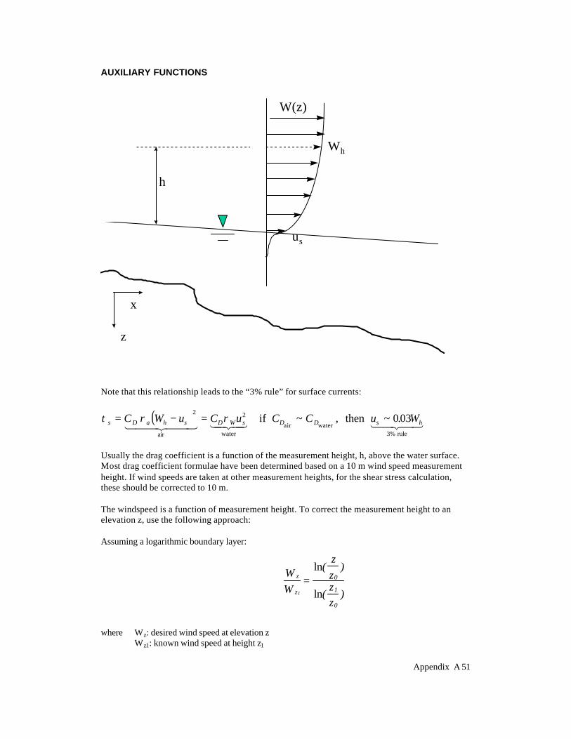
Note that this relationship leads to the “3% rule” for surface currents:

( )τ ρ ρs D a h s D W s D D s hC W u C u C C u W= − =

2 2 003air water

air water3% rule

if then 1 244 344 124 34 1 24 34~ , ~ .

Usually the drag coefficient is a function of the measurement height, h, above the water surface. Most drag coefficient formulae have been determined based on a 10 m wind speed measurement height. If wind speeds are taken at other measurement heights, for the shear stress calculation, these should be corrected to 10 m. The windspeed is a function of measurement height. To correct the measurement height to an elevation z, use the following approach: Assuming a logarithmic boundary layer:

z

z

0

1

0

WW

=(

zz

)

(zz

)1

ln

ln

where Wz: desired wind speed at elevation z Wz1: known wind speed at height z1

AUXILIARY FUNCTIONS

Appendix A 52

z0: wind roughness height (assume 0.003 ft for wind < 5 mph and 0.015 for wind > 5 mph, range 0.0005 to 0.03 ft)

This term can then be used to compute the surface stress in the direction of the x-axis and the cross-shear (the cross-shear term will be used in the turbulent shear stress algorithm) as follows:

τ ρwx D a hC W≅ −21 2cos( )Θ Θ

τ ρwy D a hC W≅ −21 2sin( )Θ Θ

where τwx: surface shear stress along x-axis due to wind τwy: surface shear stress along lateral direction due to wind Θ1: wind orientation relative to North, radians

Θ2: segment orientation relative to North, radians

North

W2 Segments

Θ2

Θ2

Θ2

n-1

n

n+1

Segments oriented fromeast to west have an angle of π/2

AUXILIARY FUNCTIONS

Appendix A 53

North

Θ1

Wh

Hence, a wind from the N would have anangle of 0, a wind from east to west would be π/2 .

The drag coefficient, CD, is defined in CE-QUAL-W2 as (note that these formulae were determined based on a 10 m measurement height): For Wh<1 m/s, CD = 0.0 For 1≤ Wh<15 m/s, CD = 0.0005(Wh)0.5 For Wh≥ 15 m/s, CD = 0.0026 Shear Stress at Bottom Boundaries The shear stress is defined along the bottom of each cell (or for each cell in contact with side walls or channel bottom) as

τρ

bw g

CU U= 2

where C is the Chezy friction coefficient U is the longitudinal velocity ρw is the density of water Also, the model user can specify a Manning’s friction factor where the Chezy coefficient is related to the Manning’s friction factor as C (for SI units only)= (1/n)R1/6

where n: Manning’s friction factor

R: hydraulic radius

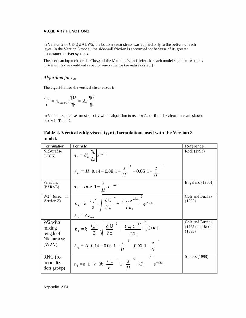
AUXILIARY FUNCTIONS

Appendix A 54

In Version 2 of CE-QUAL-W2, the bottom shear stress was applied only to the bottom of each layer. In the Version 3 model, the side-wall friction is accounted for because of its greater importance in river systems.

The user can input either the Chezy of the Manning’s coefficient for each model segment (whereas in Version 2 one could only specify one value for the entire system).

Algorithm for τxz

The algorithm for the vertical shear stress is τρ

ν∂∂

∂∂

xzturbulent z

Uz

AUz

= =

In Version 3, the user must specify which algorithm to use for Az or ν t . The algorithms are shown below in Table 2.

Table 2. Vertical eddy viscosity, ν t, formulations used with the Version 3 model.

Formulation Formula Reference Nickuradse (NICK)

−−

−−=

∂∂

= −

42

2

106.0108.014.0Hz

Hz

H

ezu

m

CRimt

l

lν

Rodi (1993)

Parabolic (PARAB) CRi

t eHz

zu −

−= 1*κν

Engelund (1976)

W2 (used in Version 2)

ee

+zU

2 )CRi(-

kz2-wy

222

∂∂

=

t

mt

lρν

τκν

maxzm ∆=l

Cole and Buchak (1995)

W2 with mixing length of Nickuradse (W2N)

e

e +zU

2 )CR i(-

kz2-wy

222

∂∂

=

t

mt

lρν

τκν

−−

−−=

42

106.0108.014.0Hz

Hz

Hml

Cole and Buchak (1995) and Rodi (1993)

RNG (re-normaliza-tion group)

CRi

t eCHz

? −

−

−

+=

3/1

1

33

* 1zu

31ν

κνν

Simoes (1998)

AUXILIARY FUNCTIONS

Appendix A 55

Formulation Formula Reference where lm: mixing length, z: vertical coordiante, H: depth, u: horizontal velocity, Ri: Richardson number, C: constant (assumed 0.15), u*: shear velocity, κ von Karman constant, τwy: cross-shear from wind, k: wave number, ρ: liquid density, ∆zmax: maximum vertical grid spacing, Ψ(x)=max(0,x), ν : molecular viscosity, C1: empirical constant (assumed 100) The model user can also specify the value of AZMAX (the maximum value of the vertical eddy viscosity), but this value is only used with the W2N and W2 formulations. This value is specified because the time step for numerical stability is greatly reduced when solving the momentum equations using an explicit numerical technique. Also, the model user can choose whether to compute the vertical momentum transfer with the longitudinal momentum equation using an implicit (IMP) or an explicit (EXP) numerical technique. The explicit formulation was used in CE-QUAL-W2 Version 2 with a fixed AZMAX of 1.0E-5 m2/s. The implicit solution code was originally developed by Chapman and Cole and revised for Version 3. Note that only the W2 and W2N include the effects of cross-shear from wind and from tributary or branch inflows. Hence, it is recommended to use either W2 or W2N for waterbodies with deep sections that could be stratified. The other formulations and should be used for estuary or river systems where the maximum computed AZMAX could be as high as 1 to 5 m2/s. For the river model, the model user should use the IMP solution technique. To reproduce results from Version 2 in a stratified reservoir, set AZMAX to 1E-5 m2/s and the calculation technique to EXP using the W2 model. How does know which turbulent closure scheme to use for τxz since according to Hamblin and Salmon (1975) "the vertical diffusion of momentum is probably the most important internal parameter" for predicting internal circulation patterns? Because of the "disarray in the literature" over which formulation is best, Shanahan (1980) suggetsed that we "use theory and literature as a guide to develop alternative viscosity functions and then test those functions in calibration runs against field data." In the absence of expensive-to-obtain current velocity data, the use of temperature profiles is often used to test the adequacy of the hydrodynamic regime against different formulations. Typical variation of these formulations, as predicted with the CE-QUAL-W2 model, is shown in Figure 28 for Manning's fiction factor and in Figure 29 for Chezy friction factor for an open-channel, non-stratified flow regime. Comparison of the various turbulence closure theories to classical open channel flow theory for 7 vertical layers is shown in Figure 30. The next sections cover the background of the various expressions for A z.

AUXILIARY FUNCTIONS

Appendix A 56

Manning's n=0.03, S=0.0001

70

72

74

76

78

80

82

84

86

0 0.05 0.1 0.15 0.2 0.25

Turbulent eddy viscosity, m2/s

PARAB

RNGW2

W2NNICK

Figure 28. Variation of turbulent vertical eddy viscosity for flow of 2574 m3/s flow down a channel of length 30 km with a slope of 0.0001 and width of 100 m at x=15 km and Manning's n=0.03.

Chezy=50 S=0.0001

70

72

74

76

78

80

82

84

86

0 0.05 0.1 0.15 0.2 0.25

Turbulent eddy viscosity, m2/s

PARAB

RNG

W2

W2N

NICK

Figure 29. Variation of turbulent vertical eddy viscosity for flow of 2574 m3/s flow down a channel of length 30 km with a slope of 0.0001 and width of 100

AUXILIARY FUNCTIONS

Appendix A 57

m measured at x=15 km and Chezy C=50.

7 vertical layers, Manning's n=0.03 S=0.0001

70

72

74

76

78

80

82

84

86

88

90

0 0.5 1 1.5 2 2.5

Current Velocity, m/s

Ele

vatio

n, m

PARABRNGW2W2NNICKTheory

Figure 30. Comparison of vertical velocity predictions of W2 model with various eddy viscosity models compared to theory.

W2 Model In CE-QUAL-W2, this shear stress term includes also the contribution to the shear stress from surface waves induced by the wind. The wind can produce waves that produce decaying motions with depth as shown below.

wind stress

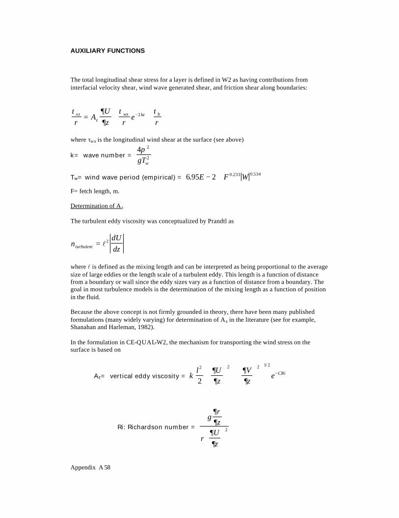
AUXILIARY FUNCTIONS

Appendix A 58

The total longitudinal shear stress for a layer is defined in W2 as having contributions from interfacial velocity shear, wind wave generated shear, and friction shear along boundaries: τρ

∂∂

τρ

τρ

xzz

wx kz bAUz

e= + +−2

where τwx is the longitudinal wind shear at the surface (see above)

k= wave number = 4 2

2

πgTw

Tw= wind wave period (empirical) = 6 95 2 0 233 0 534. . .E F W−

F= fetch length, m. Determination of A z The turbulent eddy viscosity was conceptualized by Prandtl as

νturbulent

dUdz

= l2

where l is defined as the mixing length and can be interpreted as being proportional to the average size of large eddies or the length scale of a turbulent eddy. This length is a function of distance from a boundary or wall since the eddy sizes vary as a function of distance from a boundary. The goal in most turbulence models is the determination of the mixing length as a function of position in the fluid. Because the above concept is not firmly grounded in theory, there have been many published formulations (many widely varying) for determination of Az in the literature (see for example, Shanahan and Harleman, 1982). In the formulation in CE-QUAL-W2, the mechanism for transporting the wind stress on the surface is based on

Az= vertical eddy viscosity = κ∂∂

∂∂

l Uz

Vz

e CRi2 2 2 1 2

2

+

−

/

Ri: Richardson number = g

zUz

∂ρ∂

ρ∂∂

2

AUXILIARY FUNCTIONS

Appendix A 59

κ is the von Karman constant = 0.4

C is an empirical constant taken as 1.5

l, a vertical length scale, is chosen as vertical cell thickness. Hence, this formulation is a typical mixing length formulation that is decreased or increased based on the Richardson number. The Richardson number accounts for the impact of density stratification on transfer of momentum between fluid parcels. In regions where there is no stratification, Ri=0, and the exponential term is 1. For regions where there is strong stratification

(or as ddzρ

→ ∞ ), the Richardson number becomes large and the exponential term approaches 0.

The term in the above formulation involving the lateral velocity because even winds blowing at right angles to the model cell may not cause any longitudinal velocity, but they will create a mechanism for increasing the transfer of stress vertically in the fluid. In the longitudinal-vertical model, the lateral velocity, V, and its gradient, ∂V/∂z, are due to the lateral component of wind wave motion and are assumed to be zero when averaged laterally, but not necessarily the square (∂V/∂z)2. It is assumed that cross wind shear τwy generates lateral wave components and decays exponentially with depth, z, such that τyz=τwy exp(-2kz) where τwy is the lateral wind shear at the surface (see above). Then using τ

ρ∂∂

yz

zAVz

=

The lateral velocity gradient squared becomes

∂∂

τ

ρVz

kz

Awy

z

=

−

2 2exp( )

The final equation for the vertical eddy viscosity is then

z

2 2 2wy

-2 kz

z

(-CR )A = 2

Uz

+ eA e iκ

τρ

l

∂∂

The above equation is implicit. In the model, this equation is explicit since the value of Az in the lateral wind shear term is used from the previous time step. Az is never less than the molecular kinematic viscosity for water.

AUXILIARY FUNCTIONS

Appendix A 60

RNG Turbulent Eddy Viscosity Model The RNG model was derived from the RNG model of Yakhot and Orszag (1986) by Simoes (1998). The turbulent eddy viscosity is derived from Yakhot and Orzag (1986) as

3/1

13

4

?e

1

−′Ψ+= Ca m

tl

νν

where Ψ(x)=max(0,x) ν: molecular viscosity νt: turbulent eddy viscosity

ml: mixing length

ε: turbulent energy dissipation rate a′ : constant approximately 1 C1: constant approximately 100 Two additional equations are necessary to determine the mixing length and the turbulent energy dissipation. These are

Mixing length Hz

Hz

Hm −= 1κ

l

Turbulent Eddy Dissipation

2/3

3*

13

ueH

−=

Hz

Hz

Where κ is von Karman’s constant (=0.41) Substituting these into the equation for νt,

3/1

1

33

* 1zu31

−

−

Ψ+= C

Hz

t νκνν

Simoes (1998) states that this model better represents experimental data than the more traditional parabolic eddy viscosity model of

−=

Hz

t 1?zu*ν

A value of ν was derived for this project as a function of temperature. Based on values from Batchelor (1966), a polynomial curve fit between 0 and 30oC as shown in Figure 31.

AUXILIARY FUNCTIONS

Appendix A 61

This model was adjusted by the author to account for stratified flow conditions by using the same Richardson number criteria as used in the original W2 model (the approach of Mamayev as quoted in French, 1985), i.e.,

( )CRitRNGt e −= ννν ,max

Ri: Richardson number =

gz

Uz

∂ρ∂

ρ∂∂

2

C is an empirical constant taken as 1.5 (Note that French, 1985, shows that this constant has been used as 0.4 also.) The Richardson number accounts for the impact of density stratification on transfer of momentum between fluid parcels. In regions where there is no stratification, Ri=0, and the exponential term is

1. For regions where there is strong stratification (or as

ddzρ

→ ∞), the Richardson number

becomes large and the exponential term approaches 0.

4E-7 8E-7 1.2E-6 1.6E-6 2E-6Kinematic viscosity, m2/s

0

10

20

30

40

50

Tem

pera

ture

, C

Fit Results

Fit 4: Log, Y=B*log(X)+AEquation:Y = -37.3877 * log(X) + -495.691Number of data points used = 5Average log(X) = -13.6059Average Y = 13Regression sum of squares = 577.303Residual sum of squares = 2.69662Coef of determination, R-squared = 0.995351Residual mean square, sigma-hat-sq'd = 0.898872

Fit 5: Log, Y=B*log(X)+AEquation:Y = -57.7621 * log(X) + -782.19Number of data points used = 2Average log(X) = -14.3206Average Y = 45Regression sum of squares = 50Residual sum of squares = 1.55389E-010Coef of determination, R-squared = 1

Figure 31. Variation of molecular viscosity with temperature.

Nikuradse Model

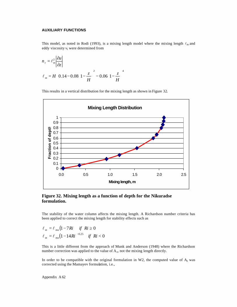
AUXILIARY FUNCTIONS

Appendix A 62

This model, as noted in Rodi (1993), is a mixing length model where the mixing length lm and eddy viscosity νt were determined from

−−

−−=

∂∂

=

42

2

106.0108.014.0Hz

Hz

H

zu

m

mt

l

lν

This results in a vertical distribution for the mixing length as shown in Figure 32.

Mixing Length Distribution

00.10.20.30.40.50.60.70.80.9

1

0.0 0.5 1.0 1.5 2.0 2.5

Mixing length, m

Fra

ctio

n o

f d

epth

Figure 32. Mixing length as a function of depth for the Nikuradse formulation.

The stability of the water column affects the mixing length. A Richardson number criteria has been applied to correct the mixing length for stability effects such as

( ) 071 ≥−= RiifRimom ll

( ) 0141 25.0 <−= − RiifRimom ll

This is a little different from the approach of Munk and Anderson (1948) where the Richardson number correction was applied to the value of Az, not the mixing length directly. In order to be compatible with the original formulation in W2, the computed value of Az was corrected using the Mamayev formulation, i.e.,

AUXILIARY FUNCTIONS

Appendix A 63

( )CRitNICKt e −= ννν ,max

Parabolic Model Another distribution is the parabolic distribution of Az (Engelund, 1978) such as

−=

Hz

zut 1*κν

Figure 33 shows the spatial distribution of A z for the parabolic model.

Vertical Eddy Viscosity Distribution

00.10.20.30.40.50.60.70.80.9

1

0.00 0.05 0.10 0.15 0.20

Eddy viscosity, m2/s

Figure 33. Variation of Az with depth for the parabolic model of Englund (1976).

In order to be compatible with the original formulation in W2, the computed value of Az was corrected also using the Mamayev formulation:

( )CRitPARABt e−= ννν ,max

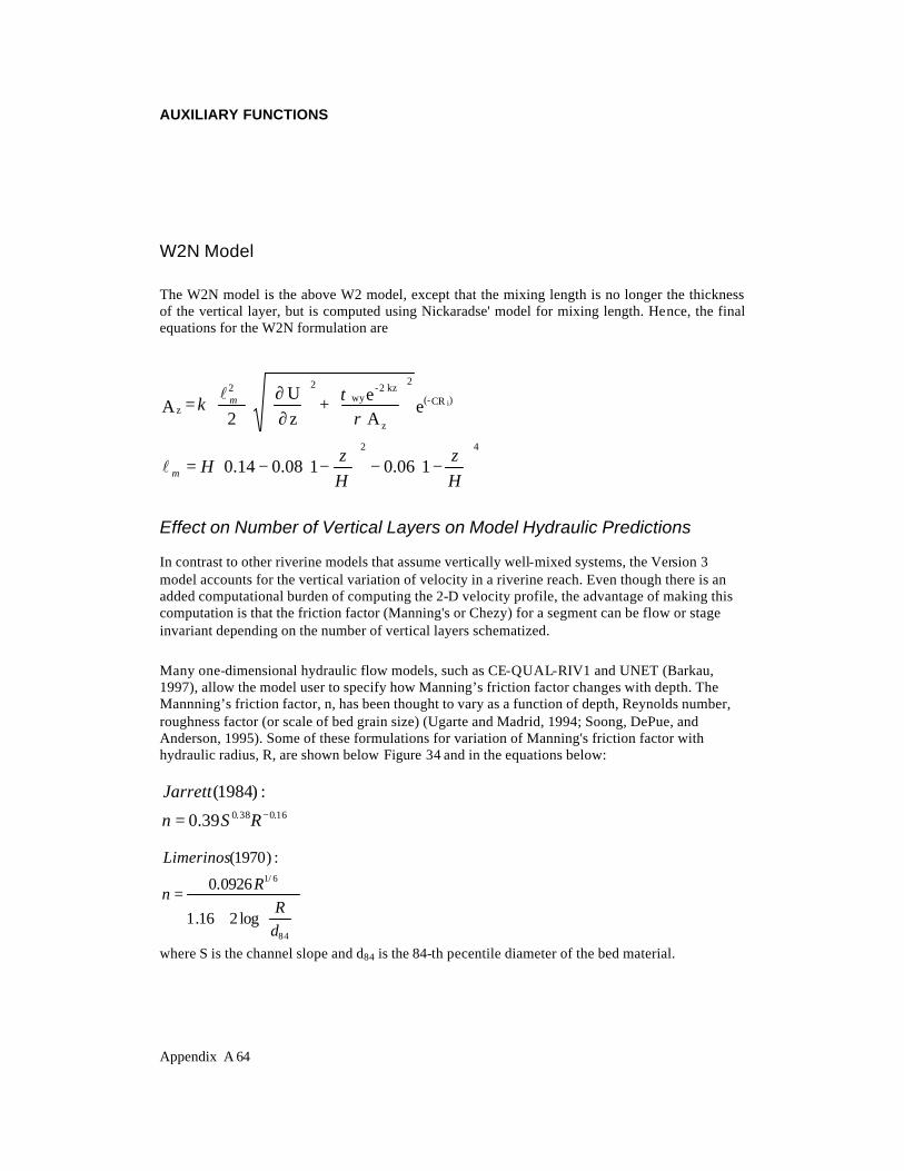
AUXILIARY FUNCTIONS

Appendix A 64

W2N Model The W2N model is the above W2 model, except that the mixing length is no longer the thickness of the vertical layer, but is computed using Nickaradse' model for mixing length. Hence, the final equations for the W2N formulation are

eAe +

zU

2 = A )CR(-

z

kz2-wy

222

zi

∂∂

ρτκ ml

−−

−−=

42

106.0108.014.0Hz

Hz

Hml

Effect on Number of Vertical Layers on Model Hydraulic Predictions In contrast to other riverine models that assume vertically well-mixed systems, the Version 3 model accounts for the vertical variation of velocity in a riverine reach. Even though there is an added computational burden of computing the 2-D velocity profile, the advantage of making this computation is that the friction factor (Manning's or Chezy) for a segment can be flow or stage invariant depending on the number of vertical layers schematized.

Many one-dimensional hydraulic flow models, such as CE-QUAL-RIV1 and UNET (Barkau, 1997), allow the model user to specify how Manning’s friction factor changes with depth. The Mannning’s friction factor, n, has been thought to vary as a function of depth, Reynolds number, roughness factor (or scale of bed grain size) (Ugarte and Madrid, 1994; Soong, DePue, and Anderson, 1995). Some of these formulations for variation of Manning's friction factor with hydraulic radius, R, are shown below Figure 34 and in the equations below:

16.038.039.0

:)1984(−= RSn

Jarrett

+

=

84

6/1

log216.1

0926.0

:)1970(

dR

Rn

Limerinos

where S is the channel slope and d84 is the 84-th pecentile diameter of the bed material.

AUXILIARY FUNCTIONS

Appendix A 65

0

1

2

3

4

5

6

7

8

0.02 0.03 0.04 0.05 0.06 0.07

Manning's friction factor

Hyd

rau

lic r

adiu

s, f

t

Limerinos (1970)Jarrett (1984)

Figure 34. Variation of Manning's friction factor using formulae from Limerinos (1970) and Jarrett (1984) for S=0.0005 and d84=50.

Researchers understand that the friction factor, when representing a hydraulic element with uniform roughness, should be flow invariant with depth (Henderson 1966). But many assert that the friction factor changes with depth because the friction coefficient is variable with the wetted perimeter. Some reason that it is to be expected that at shallow depths the larger size of the bed material produces a higher overall friction factor than a deeper flow where the side walls may have a smaller friction. Since most researchers used 1-D cross-sectionally averaged flow equations (such as Manning’s Equation, or 1-D dynamic hydraulic models), this parameterization itself has been responsible for the seeming variation of Manning’s friction factor with depth. For example, all one-dimensional hydraulic models implicitly assume that the rate of transfer of momentum from the bottom of the channel to the top is infinite. For these hydraulic models, even as the depth of the channel increases, these models still assume an infinite rate of transfer of momentum from the channel bottom to the surface. Hence, as the water depth increases, the apparent friction factor must be reduced because of the assumption of infinite momentum transfer between the bed and the water surface. But, in a 2-D (vertical-longitudinal) river model, the Manning's friction factor does not have to be varied with stage in order to produce the effect that as the river stage increases, the apparent friction decreases. The water surface set-up changes significantly as the layer numbers increase. In general, the water surface slope increases as the number of computational layers decreases. In other words, the average eddy viscosity in the water column increases as the number of layers decrease until at the limit of a one-layer system, the average vertical eddy viscosity is infinite. The fact that the Manning’s friction factor seems to decrease with depth in 1-D models is accounted for in modeling the river channel as a 2-D (vertical-longitudinal) system.

AUXILIARY FUNCTIONS

Appendix A 66

CE-QUAL-W2 Version 3 uses five different vertical eddy viscosity formulations. These formulations were shown earlier in Table 2. Typical variation of these formulations, as predicted with the CE-QUAL-W2 model, was shown in Figure 30 for Manning's fiction factor for an open-channel, non-stratified flow regime as compared to theory of steady uniform channel flow. The number of vertical layers significantly affected the model predictions. For example, Figure 35 shows a comparison of vertical velocity profiles from a model with 1, 3 and 7 vertical layers using the PARAB eddy viscosity model. .

S=0.001, Q=2574 m3/s, n=0.03, PARAB

70

72

74

76

78

80

82

84

86

0 0.5 1 1.5 2 2.5

Velocity, m/s

Ele

vatio

n, m

3-layer7-layer1-layer

Figure 35. Comparison of vertical velocity predictions of W2 model with 1, 3 and 7 vertical layers Figure 36 shows how the change in the number of vertical layers affects the water surface slope over the domain length for a steady-state flow. In order to model the water surface slope of the 1-layer model with the 7-layer model, the apparent value of Manning's friction factor would have to be reduced. Hence, the apparent friction decreases as the number of layers increase.

AUXILIARY FUNCTIONS

Appendix A 67

CE-QUAL-W2 V3 was also compared to the 1-D models DYNHYD (Ambrose et al., 1988) and CE-QUAL-RIV1 (Environmental Laboratory, 1995) by running W2 with only a single vertical layer.

Q=2574 m3/s, S=0.0001, n=0.03

2.88

2.89

2.9

2.91

2.92

2.93

2.94

0 2 4 6 8

# of vertical layers

Ele

vati

on

dro

p o

ver

30 k

m d

ista

nce

, m

Figure 36. Comparison of elevation drop of W2 model with 1, 3 and 7 vertical layers with same Manning's friction factor.

The average velocities between the 3 models agreed well with theory but the water surface slopes were different. The W2 model predicted an elevation difference of 2.93 m, compared to 2.07 m for DYNHYD and 2.05 m for RIV1 over 30 km for a Q=2574 m3/s, n=0.03, S=0.001, and channel width=100 m. Based on classical steady-state theory, the actual difference should have been 2.9 m. Both the DYNHYD and RIV1 models required friction factors greater than expected to correspond to classical theory. This may have been a result of these models not incorporating side-wall friction which was important during these test runs where the depth was 15 m and the width was 100 m.

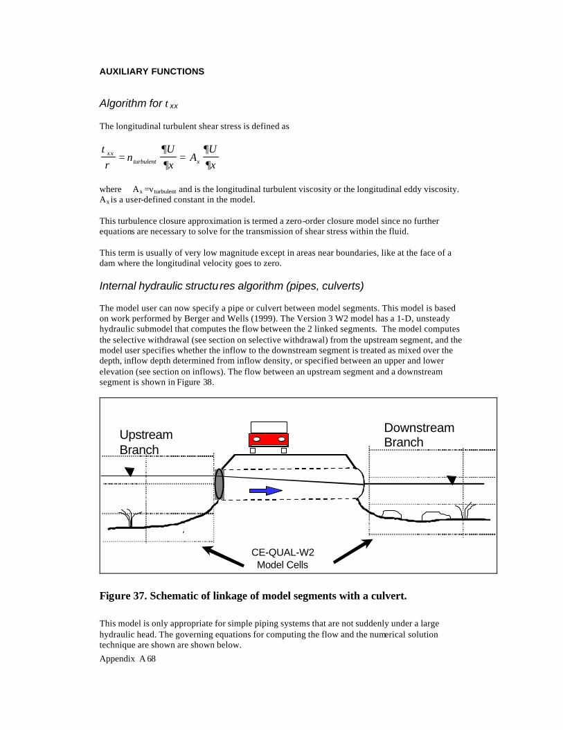
AUXILIARY FUNCTIONS

Appendix A 68

Algorithm for τxx The longitudinal turbulent shear stress is defined as τρ

ν∂∂

∂∂

xxturbulent x

Ux

AUx

= =

where Ax =νturbulent and is the longitudinal turbulent viscosity or the longitudinal eddy viscosity. Ax is a user-defined constant in the model. This turbulence closure approximation is termed a zero-order closure model since no further equations are necessary to solve for the transmission of shear stress within the fluid. This term is usually of very low magnitude except in areas near boundaries, like at the face of a dam where the longitudinal velocity goes to zero. Internal hydraulic structu res algorithm (pipes, culverts) The model user can now specify a pipe or culvert between model segments. This model is based on work performed by Berger and Wells (1999). The Version 3 W2 model has a 1-D, unsteady hydraulic submodel that computes the flow between the 2 linked segments. The model computes the selective withdrawal (see section on selective withdrawal) from the upstream segment, and the model user specifies whether the inflow to the downstream segment is treated as mixed over the depth, inflow depth determined from inflow density, or specified between an upper and lower elevation (see section on inflows). The flow between an upstream segment and a downstream segment is shown in Figure 38.

UpstreamBranch

DownstreamBranch

CE-QUAL-W2 Model Cells

Figure 37. Schematic of linkage of model segments with a culvert. This model is only appropriate for simple piping systems that are not suddenly under a large hydraulic head. The governing equations for computing the flow and the numerical solution technique are shown are shown below.

AUXILIARY FUNCTIONS

Appendix A 69

The governing equations used to predict flow through culverts were the one-dimensional time-dependent conservation of momentum and continuity equations (Yen, 1973).

( ) 0cos =−−−++ mfo SSSgxh

gxu

utu

∂∂

φ∂∂

∂∂

∂∂

∂∂

∂∂

ht

uhx

AT

ux

+ + = 0

where u - velocity t - time h – piezometric head g - gravitational acceleration x - distance along axis of culvert A - cross-sectional area of culvert filled with water T - width of water level surface φ - angle between culvert axis and horizontal

So - culvert slope

S f - friction slope.

mS - minor loss slope

The friction slope S f was estimated with the Manning formula

Sn

Ruuf =

2

43

n - Mannings roughness factor R - hydraulic radius. Minor losses due to entrance configuration, gates, valves, and corners were accounted for in the minor loss term mS where

Lg

uukSm

12

=

and k - sum of minor loss coefficients L - length. Pressurized or full culvert flow was modeled assuming a fictitious water surface width called a Preissmann slot (Yen, 1986). If the culvert was full, the surface width T was zero and the governing equations became singular. Using a Preissmann slot avoided having to switch between the open channel and pressurized flow equations. The slot must be narrow enough to minimize error in the mass and momentum balance but large enough to maintain numerical stability when solving the open channel St. Venant equations. A top width of 0.5% of the diameter was assumed for culverts flowing full. The advantages of using a Preissmann slot were quoted in Yen (1986):

AUXILIARY FUNCTIONS

Appendix A 70

(a) It uses only Saint-Venant equations and avoids switching between the surcharge equation and open-channel flow equations and avoids the associated separate treatment of the boundary conditions.

(b) There is no need to define surcharge criteria (c) It is not necessary to keep inventory of the pipes that are surcharged at different times. (d) It permits the flow transition to progress computationally reach by reach in a sewer, as in

the open-channel case, and hence it can account for the situation when only part of the length of the pipe is full.

(e) It requires few additional assumptions than the standard approach to achieve numerical stability

(f) It is simpler in programming. along with the some potential disadvantages:

(a) It introduces a potential accuracy problem in the mass and momentum balance of the flow if the slot is too wide, and stability problems if it is too narrow.

(b) It sill requires computation of two equations (continuity and momentum) for each of the reaches of the sewer when the sewer is full surcharged, whereas in the standard surcharge computation only one equation is applied to the entire length of the sewer

(c) It is hypothetical rather than real. The Preissmann slot concept has been applied to other models for surcharged flow including the model described by Abbot (1982) and SWMM EXTRAN (Roesner et al. 1988). The boundary condition used for solving the governing equations was the head or water level at each end of the culvert. However, if the water level at the downstream end of the culvert was less than the critical depth, the critical depth was used. Momentum was not transferred between CE-QUAL-W2 model segments and the culverts. Initial conditions were the calculated velocities and heads of the previous time step. The governing equations cannot be solved analytically and an implicit finite difference scheme was used to approximate the solution. The solution method employed the “leap-frog scheme” which calculates the head and velocity at alternating computational nodes. The finite difference forms of the continuity and momentum equations were

0)1(2

)1(2

1111

1122

12

12

1

=∆

−−+

∆

−+

∆

−−+

∆

−+

∆

− −++−

++−+

+−

++

+

x

uu

T

A

x

uu

T

A

x

hhu

x

hhu

t

hh nj

nj

nj

nj

nj

nj

nj

nj

nj

njn

j

nj

njn

j

nj

nj θθθθ

0)1()1(

)1()1(

1111111

34

2

111

34

2

211

2111

11

11

1

1

=−++−+

+∆

−−+

∆

−+

∆

−−+

∆

−+

∆

−

++++++++

++

+++

+−++

+−

++

+

+

nj

nj

nj

nj

nj

nj

nj

nj

nj

nj

nj

nj

nj

njn

j

nj

njn

j

nj

nj

uuLk

uuLk

uuR

nguu

R

ng

x

hhg

x

hhg

x

uuu

x

uuu

t

uu

θθθθ

θθθθ

where the n-index references time step and the j subscript references the spatial node. Figure 38 compares flow predictions using the dynamic culvert model with flow data taken within a culvert at NE 47th bridge in the Upper Columbia Slough, Portland, Oregon. Data was recorded by a flow meter (Flow-Tote) placed directly in a culvert. The cyclical flows are the result of turning pumps on and off at MCDD#1, a downstream pump station. The culvert was calibrated by adjusting the minor loss parameter.

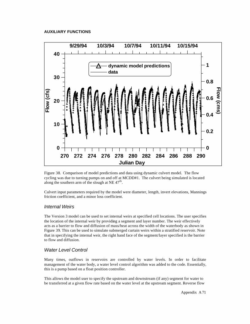
AUXILIARY FUNCTIONS

Appendix A 71

270 272 274 276 278 280 282 284 286 288 290Julian Day

0

10

20

30

40Fl

ow (

cfs)

dynamic model predictionsdata

9/29/94 10/3/94 10/7/94 10/11/94 10/15/94

0

0.2

0.4

0.6

0.8

1

Flow (cm

s)

Figure 38. Comparison of model predictions and data using dynamic culvert model. The flow cycling was due to turning pumps on and off at MCDD#1. The culvert being simulated is located along the southern arm of the slough at NE 47th. Culvert input parameters required by the model were diameter, length, invert elevations, Mannings friction coefficient, and a minor loss coefficient. Internal Weirs The Version 3 model can be used to set internal weirs at specified cell locations. The user specifies the location of the internal weir by providing a segment and layer number. The weir effectively acts as a barrier to flow and diffusion of mass/heat across the width of the waterbody as shown in Figure 39. This can be used to simulate submerged curtain weirs within a stratified reservoir. Note that in specifying the internal weir, the right hand face of the segment/layer specified is the barrier to flow and diffusion. Water Level Control Many times, outflows in reservoirs are controlled by water levels. In order to facilitate management of the water body, a water level control algorithm was added to the code. Essentially, this is a pump based on a float position controller. This allows the model user to specify the upstream and downstream (if any) segment for water to be transferred at a given flow rate based on the water level at the upstream segment. Reverse flow

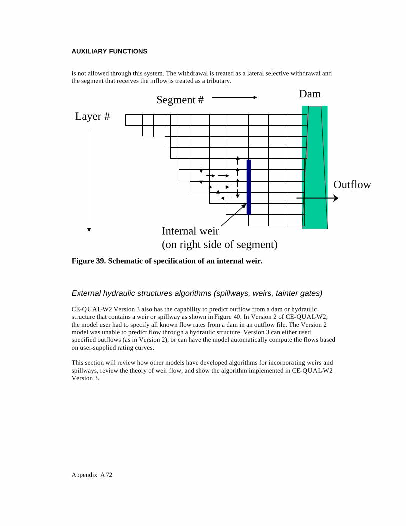
AUXILIARY FUNCTIONS

Appendix A 72

is not allowed through this system. The withdrawal is treated as a lateral selective withdrawal and the segment that receives the inflow is treated as a tributary.

Segment #Layer #

Internal weir(on right side of segment)

Dam

Outflow

Figure 39. Schematic of specification of an internal weir.

External hydraulic structures algorithms (spillways, weirs, tainter gates) CE-QUAL-W2 Version 3 also has the capability to predict outflow from a dam or hydraulic structure that contains a weir or spillway as shown in Figure 40. In Version 2 of CE-QUAL-W2, the model user had to specify all known flow rates from a dam in an outflow file. The Version 2 model was unable to predict flow through a hydraulic structure. Version 3 can either used specified outflows (as in Version 2), or can have the model automatically compute the flows based on user-supplied rating curves. This section will review how other models have developed algorithms for incorporating weirs and spillways, review the theory of weir flow, and show the algorithm implemented in CE-QUAL-W2 Version 3.

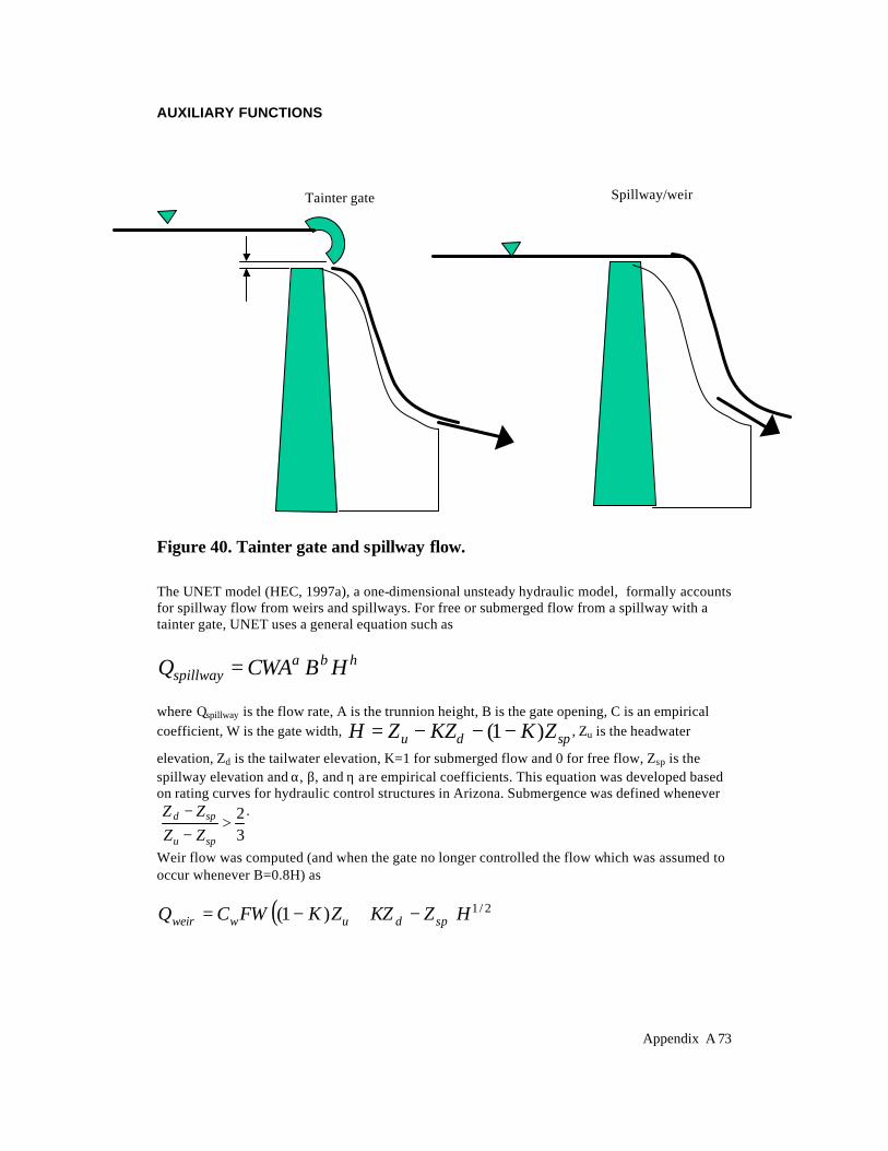
AUXILIARY FUNCTIONS

Appendix A 73

Figure 40. Tainter gate and spillway flow. The UNET model (HEC, 1997a), a one-dimensional unsteady hydraulic model, formally accounts for spillway flow from weirs and spillways. For free or submerged flow from a spillway with a tainter gate, UNET uses a general equation such as

ηβα HBCWAQspillway =

where Qspillway is the flow rate, A is the trunnion height, B is the gate opening, C is an empirical coefficient, W is the gate width, spdu ZKKZZH )1( −−−= , Zu is the headwater

elevation, Zd is the tailwater elevation, K=1 for submerged flow and 0 for free flow, Zsp is the spillway elevation and α, β, and η are empirical coefficients. This equation was developed based on rating curves for hydraulic control structures in Arizona. Submergence was defined whenever

32>

−−

spu

spd

ZZZZ .

Weir flow was computed (and when the gate no longer controlled the flow which was assumed to occur whenever B=0.8H) as

( ) 2/1)1( HZKZZKFWCQ spduwweir −+−=

Tainter gate Spillway/weir

AUXILIARY FUNCTIONS

Appendix A 74

where Cw is the weir coefficient, [ ][ ]

−

−−=

spu

spd

ZZ

ZZF 13

when K=1; and F=1 when K=0. For a

concrete spillway HEC (1997a) suggests using a value of Cw of 4. Note that the above 2 equations are considered equivalent whenever B=0.8H. The steady-one-dimensional steady-state hydraulic model, HEC-RAS (HEC, 1997b), includes the capability to model the flow over spillways, including gated spillways (tainter gates and sluice gates), broad-crested weirs, or an ogee crest. Ineffective flow area is used to block a part of the channel until it reaches the level of a spillway or weir. A summary of the equations used by HEC-RAS as well as explanations are shown in Table 3.

Table 3. HEC-RAS (HEC, 1997b) flow rates through weirs and sluice gates.

Condition Equation Description Radial flow gate, flowing freely

HEBETE HBWTgCQ 2= When the upstream water surface is ≥1.25 times the gate opening height (above the spillway crest), Q is the flow in cfs, C is discharge coefficient (between 0.6 and 0.8), W is the width of the gated spillway in ft, T is the trunnion height (from spillway crest to trunnion pivot point) in ft, B height of gate opening in ft, H is the upstream energy head above spillway crest Zu-Zsp, Zu is the elevation of the upstream energy grade line, Zd is the downstream water surface, Zsp is the elevation of the spillway crest, TE is an empirical trunnion height exponent (0.16), BE is the gate opening coefficient (0.72) and HE is the head exponent (0.62).

radial gate flowing under submerged conditions

HEBETE HBWTgCQ 23=

When the upstream water surface is ≥1.25 times the gate opening height (above the spillway crest), whenever the tailwater depth divided by the energy depth above the spillway is greater than 0.67, H is now defined as Zu-Zd

freely flowing sluice gate WBgHCQ 2= When the upstream water surface is ≥1.25 times the

gate opening height (above the spillway crest), H is the upstream energy head above the spillway = Zu-Zsp, and C is a discharge coefficient (0.5 to 0.7)

submerged sluice gate WBgHCQ 23= When the upstream water surface is ≥1.25 times the

gate opening height (above the spillway crest), whenever the tailwater depth divided by the energy depth above the spillway is greater than 0.67, H is Zu-Zd

Low flow through gated structure

2/3CLHQ = When upstream water level is equal to or less than the top of the gate opening, weir flow equation is used, C is the weir coefficient and ranges from 2.6 to 4.0 depending on broad crested or Ogee spillway, length of spillway crest, H is the upstream energy head above the spillway crest, for an Ogee spillway the value of C is adjusted according to a 1977 Bureau of Reclamation study on variability of C for Ogee spillways, suggested

AUXILIARY FUNCTIONS

Appendix A 75

Condition Equation Description values of C are 2.6 for bridge decks and 3.0 for flow over elevated roadways

Flow over Weirs Analysis of flow over weirs has been studied extensively. Martin and McCutcheon (1999) show that a typical relationship between the pool depth and flow over a weir is

ηwce hWCQ =

where Ce and η are empirical coefficients, Wc is the length of the weir crest and hw is the height of the pool above the weir crest. Theoretical calculations of steady-state flow over a weir can be complex depending on whether the weirs are sharp-crested, broad-crested, V-notched, rectangular, Cipolletti, parabolic, or some other type. Table 4 shows some examples from French (1985) and USBR (1999) on typical equations used for the different weir types. For many regular weir types, formulae exist for accurate estimation of the flow. But in most cases, a rating curve for a given installation is necessary beacuase of the uncertainty of end effects, flow alignments, shallowness in the upstream pool, and other unique features of the installation (Martin and McCutcheon, 1999).

Table 4. List of weir types (after French, 1985, and USBR, 1999)

Weir type Weir Equation Description Rectangular broad crested weir

2/313

232

WhgCCQ vD= Valid when 0.08 <H1/L<0.5 where H1 is the total head upstream of the weir (energy + static head) and L is the length of the weir block, W is the width of the rectangular weir from edge to edge, Cv varies from 1 to 1.2 and CD varies from 0.85 to 1.06

Rectangular, sharp crested weir

2/312

32 BhgCQ e= Olson and Wright (1990) show that Ce

depends on the approach velocity head, V2/2g and the contraction of streamlines just beyond the weir crest and show that Ce is of the form: Ce=0.611+0.075*(H/Z) where H is the weir head and Z is the weir crest head (as measured from the bottom of a channel); Clay (1995) suggests a simple equation of Q=3.33BH3/2 of this form when approach velocities are less than 1 fps or Q=3.33B[(H+h)3/2-hv

3/2] where hv=V2/2g and V is the approach velocity

Parabolic, broad-crested 2

143 hfgCCQ vD=

f is the distance from the bottom point of the weir to the weir focal point

Parabolic, sharp-crested

212

1 hfgCQ e π=

Triangular, broad-crested

2/51)5.0tan(

52

2516 hgCCQ vD Θ= Theta is the angle of half of the triangular weir

AUXILIARY FUNCTIONS

Appendix A 76

Weir type Weir Equation Description Triangular, sharp-crested

2/51)5.0tan(2

258 hgCQ e Θ= Ce is a function of notch angle and varies from

0.59 to 0.57 for angles between 20 and 100 degrees

Trapezoidal, broad-crested

[ ] 2/11

2 )(2)( cccD yHgmyTyCQ −+=

T is the top width, m is the slope, yc is the water surface elevation at the weir, H1 is the energy head upstream of the spillway

Trapezoidal, sharp-crested

2/111 )5.0tan

54

(232

hhbgCQ e Θ+=

Theta is the angle of the trapezoid at a convergence point of the 2 sides

Truncated triangular, broad-crested

2/31 )5.0(

32

32

bvD HhTgCCQ −=

When H1 > 1.25Hb, otherwise use equation for broad crested triangular weir, Hb is the depth from the bottom of the truncated triangular weir to the top of the triangle and the beginning of the rectangular section

Truncated triangular, sharp-crested

))((2154 5.2

15.2

1 bb

e HhhHT

gCQ −−=

When H1 > Hb, otherwise use equation for sharp crested triangular weir

Cipoletti 2/312

32

WhgCCQ vD= A modification of the contracted, rectangular, sharp-crested weir with a trapezoidal control section and sides sloping outward with slopes of 4:1; CD≅0.63 and Cv varies from 1 to 1.2 and is a function of CD and the ratio of area upstream of the control section and at the control section

Proportional or sutro weir )

31(2 1 ahgabCQ D −= Where a is the height of the rectangular

portion of the weir above the base, and b is the width of the bottom of the sutro weir, CD varies from 0.597 to 0.619 for symmetrical Sutro weir and between 0.625 and 0.603 for unsymmetrical Sutro weir

CE-QUAL-W2 Version 3 Implementation Since all weirs in practice are calibrated and a head discharge relationship is usually determined, CE-QUAL-W2 accepts only the Q vs H relationship rather than an equation from Table 4. The model user then must analyze the weir or spillway and input a relationship based on the weir or spillway geometry. The model accepts equations in the form of a power function:

11

βα hQ ∆= for freely flowing conditions

where α1, β1 are empirical parameters and ∆h is Zu-Zsp, Zu is the upstream head, and Zsp is the spillway crest elevation and

AUXILIARY FUNCTIONS

Appendix A 77

22

βα hQ ∆= for submerged conditions

where α2, β2 are empirical parameters and ∆h is Zu-Zd, Zu is the upstream head, and Zd is the downstream head. Submerged conditions are defined as whenever the tailwater depth over the upstream energy head (static head and velocity head) is greater than 0.67 (HEC, 1997b). Even though negative flow rates are possible using the second equation whenever Zd>Zu , these results should be used with caution since rarely are ratings curve done for reverse flow over a spillway. The model user needs to insure that there is a smooth transition between submerged flow conditions and free flowing conditions by proper choice of model coefficients. This means that calculations should be made to show that at the transition from free flowing to submerged flow conditions there is a relatively smooth flow transition. This is illustrated in Figure 41.

-3 -2 -1 0 1 2 3 4 5 6 7

Flow rate, m3/s

-2

0

2

4

6

Hea

d di

ffer

ence

from

ups

tream

to ta

ilwat

er, m

Free flow condition

Submerged flow condition

Reverse flow when tailwater elevation greater than upstream elevation

Figure 41. Flow rate over a spillway or weir for submerged and free flow conditions.

These equations above are only for uncontrolled weirs without gates. For a gated structure or sluice gate, a more complex rating curve is required based on the opening of the gate or sluice and the head difference between the upstream and downstream condition (the spillway crest if free flow and the tailwater elevation if submerged flow). For a freely flowing condition, CE-QUAL-W2 uses the following equation:

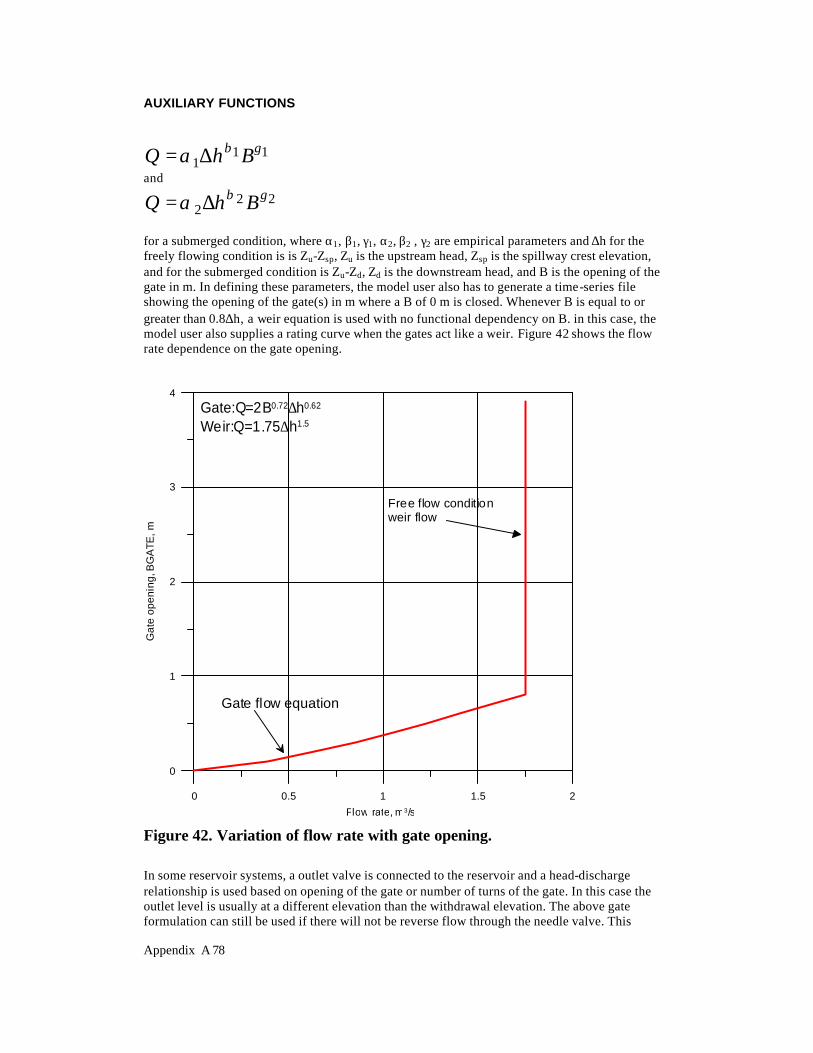
AUXILIARY FUNCTIONS

Appendix A 78

111

γβα BhQ ∆=

and

222

γβα BhQ ∆=

for a submerged condition, where α1, β1, γ1, α2, β2 , γ2 are empirical parameters and ∆h for the freely flowing condition is is Zu-Zsp, Zu is the upstream head, Zsp is the spillway crest elevation, and for the submerged condition is Zu-Zd, Zd is the downstream head, and B is the opening of the gate in m. In defining these parameters, the model user also has to generate a time-series file showing the opening of the gate(s) in m where a B of 0 m is closed. Whenever B is equal to or greater than 0.8∆h, a weir equation is used with no functional dependency on B. in this case, the model user also supplies a rating curve when the gates act like a weir. Figure 42 shows the flow rate dependence on the gate opening.

0 0.5 1 1.5 2

Flow rate, m3/s

0

1

2

3

4

Gat

e op

enin

g, B

GA

TE, m

Free flow conditionweir flow

Gate flow equation

Gate:Q=2B0.72∆h0.62

Weir:Q=1.75∆h1.5

Figure 42. Variation of flow rate with gate opening. In some reservoir systems, a outlet valve is connected to the reservoir and a head-discharge relationship is used based on opening of the gate or number of turns of the gate. In this case the outlet level is usually at a different elevation than the withdrawal elevation. The above gate formulation can still be used if there will not be reverse flow through the needle valve. This

AUXILIARY FUNCTIONS

Appendix A 79

situation is illustrated in Figure 43. In this case, the elevation of the outflow is required in addition to the elevation at which the outflow is taken if a rating curve is used in the model. The use of this is described in the section on changes to the control file. W2 currently does not have the ability to

decide the distribution of outflows if more than one selective withdrawal gate is open.

Figure 43. Selective withdrawal with outflow connected to a valve with a gate. The model user can insert weirs and/or spillways, specify connectivity to other model segments, and insert the ratings curve parameters for each weir/spillway. The model treats each spillway or weir or gate as a selective withdrawal outflow and uses the selective withdrawal algorithm for determining water flow from each vertical layer adjacent to the structure. Inflows from hydraulic control structures are treated as tributary inflows where the user must specify whether the inflow is placed according to density, equally distributed between all vertical layers, or distributed between a given elevation range. If a valve rating curve is used as a "gate" and the outlet elevation to compute the head difference is not the same at the withdrawal elevation the following changes are made above. The section “GATE WEIR” present weir equations used when the gates are open and the open gate does not interfere with the flow and hence weir flow is assumed through the gates (when

hB ∆≥ 8.0 ).

Gate valve

Selective withdrawal

dam

AUXILIARY FUNCTIONS

Appendix A 80

Conservation of longitudinal momentum at branch intersections Version 3 allows the conservation of longitudinal momentum at branch intersections (see Figure 44). The model user does not need to account for this explicitly since this is done automatically in the code. The vector component of velocity in the x-direction of the main channel, Ux, can be computed by analysis of the channel orientations. This component in the x-direction would be: Ux=Ucosβ where U is the longitudinal velocity of the tributary at the downstream segment that intersects the main branch and β is the difference in the angle between the main stem and tributary segments.

θ2 main stem

θ2 tributary branch

x

x U Uy

Ux

N

Figure 44. Schematic of branch connection. The conservation of momentum about a control volume, the main stem segment, would result in an additional source of momentum. Lai (1986) shows that the correction to the x-momentum equation would be: qBU x where q is the lateral inflow per unit length. This arises from re-deriving the momentum equations and assuming that all the fluid (q) entering the segment is moving at the velocity Ux. This correction to the x-momentum equation would be

∂∂

∂∂

∂∂

+ −

∂∂

∂∂

+

∫UB

t +

UUBx

+ WUB

z = sin cos

cos +

x

+ B

zx

gB g Bx

g Bx

dz

BqBU

z

xx zx

α α∂η∂

αρ

∂ρ∂

ρτ

ρτ

η

1 1

momentum from side tributaries123

AUXILIARY FUNCTIONS

Appendix A 81

Increased vertical mixing from lateral inflows Wells (1997) proposed accounting for the cross-shear as a result of the y component of the velocity of a side branch in the computation of the vertical eddy viscosity (and as a result the vertical diffusivity). This was implemented by increasing the cross-shear velocity gradient. In W2 Version 2 wind shear across the lateral axis of a segment also increased the vertical mixing by affecting the computation of Az. Analogous to the shear from wind, an additional side shear was implemented in the calculation of Az, the vertical eddy diffusivity coefficient, in Version 3 as follows:

eA

e +

zU

2 = A )CR(-

z

kz2-wy

222

zi

+

∂∂

ρ

ττκ ytributaryl

where

2

8 yi

ytributary Uf

ρτ ≅, fi is an interfacial friction factor (about 0.01)

xz

QU yin

y ∆∆=

∑

[ ] [ ]∑∑ +∆= stributarieybranchin QzBUQy

Ubranchy =Ubranchsin(Θmain-Θbranch) ∆z is the layer height of the receiving segment's layer B is the layer width of the receiving segment's layer ∆x is the longitudinal spacing of the cell in the main branch receiving the inflow Qtributaries is the flow rate of tributaries (assumed to be at right angles to the main channel). This side shear effect is only computed when the vertical mixing algorithm chosen by the user is W2 or W2N. Heat Budget Surface Heat Exchange. Surface heat exchange can be formulated as a term by-term process using the explicit adjacent cell transport computation as long as the integration timestep is shorter than or equal to the frequency of the meteorological data. Surface heat exchange processes depending on water surface temperatures are computed using previous timestep data and are therefore lagged from transport processes by the integration timestep. Term-by-term surface heat exchange is computed as:

(A-46)

where Hn = the net rate of heat exchange across the water surface, W m-2 Hs = incident short wave solar radiation, W m-2 Ha = incident long wave radiation, W m-2 Hsr = reflected short wave solar radiation, W m-2

n s a e c sr ar brH = H + H + H + H - ( H + H + H )

AUXILIARY FUNCTIONS

Appendix A 82

Har = reflected long wave radiation, W m-2 Hbr = back radiation from the water surface, W m-2 He = evaporative heat loss, W m-2 Hc = heat conduction, W m-2 The short wave solar radiation is either measured directly or computed from sun angle relationships and cloud cover. The long wave atmo spheric radiation is computed from air temperature and cloud cover or air vapor pressure using Brunts formula. The right-hand terms are all water surface temperature dependent. Water surface back radiation is computed as:

where E = emissivity of water, 0.97 σ* = Stephan-Boltzman constant, 5.67 x 10-8 W m-2 °K-4 Ts = water surface temperature, °C Like the remaining terms, it is computed for each surface layer cell on each iteration timestep. Evaporative heat loss is computed as:

where f(W) = evaporative wind speed function, W m-2 mm Hg-1 es = saturation vapor pressure at the water surface, mm Hg ea = atmo spheric vapor pressure, mm Hg Evaporative heat loss depends on air temperature and dew point temperature or relative humidity. Surface vapor pressure is computed from the surface temperature for each surface cell on each iteration. Surface heat conduction is computed as:

where Cc = Bowen's coefficient, 0.47 mm Hg °C-1 Ta = air temperature, °C Short wave solar radiation penetrates the surface and decays exponentially with depth according to Bears Law:

where Hs(z) = short wave radiation at depth z, W m-2 β = fraction absorbed at the water surface

br*

s4H = (T + 273.15)ε σ (A-47)

e s aH = f(W) (e - e ) (A-48)

c c s aH = C f(W) (T - T ) (A-49)

s s- zH (z) = (1 - ) H eβ η (A-50)

AUXILIARY FUNCTIONS

Appendix A 83

η = extinction coefficient, m-1 Hs = short wave radiation reaching the surface, W m-2 Aside from the problems of measuring meteorological data relative to a large waterbody and especially the problem of translating climatological data from distant weather stations, the most uncertain parame ter in the surface heat exchange computations is the evaporative wind speed function, f(W). Various formulations of f(W) have been catalogued and examined in Edinger, et al. (1974). Unlike the use of wind speed in wind shear relations as discussed in the previous section, evaporative wind speed is thought to be a "ventila tion speed" rather than a vector velocity. The different formulations result from the empirical determination of f(W) for different size and shape waterbodies with data from different locations and averaged over different periods of time. Since certain of the terms in equation (A-46) are surface temperature dependent, and others are measurable or computable input variables, the most direct route is to define an equilibrium temperature, Te, as the temperature at which the net rate of surface heat exchange is zero. Equilibrium temperature is the fictitious water surface temperature at which incoming radia tion heat rates are just balanced by outgoing water surface temperature dependent processes. Linearization of equation (A-46) along with the definition of equilibrium temperature allows expressing the net rate of surface heat exchange, Hn, as:

where Hn = rate of surface heat exchange, W m-2 Kaw = coefficient of surface heat exchange, W m-2 °C-1 Tw = water surface temperature, °C Te = equilibrium temperature, °C Seven separate heat exchange processes are summarized in the coefficient of surface heat exchange and equilibrium tempera ture. The lineariza tion used in obtaining equation (A-51) has been examined in detail by Brady, et al. (1968), and Edin ger et al. (1974). The definition of the coefficient of surface heat exchange can be shown to be the first term of a Taylor series expansion by considering equation (A-51) as: where the derivative of Hn with respect to surface temperature is evaluated from equation (A-46)

to give Kaw, the coefficient of surface heat exchange. All approximations of the individual surface heat exchange terms enter into the evaluation of the coefficient of surface heat exchange and the equilibrium temperature. Equations (A-47) and (A-48) are defined from equation (A-46). They have the same difficulties in evaluation as the individual terms in equation (A-46), but provide a simpler algebra ic method for including surface heat exchange in temperature analyses. The mass evaporation rate is computed by dividing evaporative heat loss by the latent heat of evaporation of water. Surface heat exchange always includes evaporative heat loss in the heat budget, but the user may choose to exclude it in the water budget. For many reservoirs, inflow rates are determined from storage estimates that implicitly include evaporation.

n aw w eH = - K (T - T ) (A-51)

nn

ss eH = - dH

dT ( T - T ) (A-52)

AUXILIARY FUNCTIONS

Appendix A 84

Sediment Heat Exchange. Sediment heat exchange with water is generally small compared to surface heat exchange and many previous modelers have neglected it. Investigations on several reservoirs have shown the process must be included to accurately reproduce hypolimnetic temperatures primarily because of the reduction in numerical diffusion. The formulation is similar to surface heat exchange:

where Hsw = rate of sediment/water heat exchange, W m-2 Ksw = coefficient of sediment/water heat exchange, W m-2 °C-1 Tw = water temperature, °C Ts = sediment temperature, °C Previous applications used a value of 7 x 10-8 W m-2 °C-1 for Ksw which is approximately 2 orders of magnitude smaller than the surface heat exchange coefficient. Average yearly air temperature is a good estimate of Ts.

Ice Cover Ice thickness and onset and loss of ice cover play an important role in the heat budget of northern waterbodies. At high latitudes, ice cover may remain until late spring or early summer and prevent warming due to absorption of short wave solar radiation. The ice model is based on an ice cover with ice-to-air heat exchange, conduction through the ice, conduction between underlying water, and a "melt temperature" layer on the ice bottom (Ashton, 1979). The overall heat balance for the water-to-ice-to-air system is:

where ρ i = density of ice, kg m-3 Lf = latent heat of fusion of ice, J kg-1 ∆h/∆t = change in ice thickness (h) with time (t), m sec-1 hai = coefficient of ice-to-air heat exchange, W m-2 °C-1 hwi = coefficient of water-to-ice heat exchange through the melt layer, W m-2 C- Ti = ice temperature, °C Tei = equilibrium temperature of ice-to-air heat exchange, °C Tw = water temperature below ice, °C Tm = melt temperature, 0°C The ice-to-air coefficient of surface heat exchange, hai, and its equilibrium temperature, Tei, are computed the same as for surface heat exchange in Edin ger, et al. (1974) because heat balance of the thin, ice surface water layer is the same as the net rate of surface heat exchange presented previously. The coefficient of water-to-ice exchange, hwi, depends on turbulence and water movement under ice and their effect on melt layer thickness. It is a function of water velocity for rivers but must be empirically adjusted for reservoirs.

sw sw w sH = - K (T - T ) (A-53)

i f ai i e wi w m L ht

= h (T - T ) - h (T - T )ρ∆∆

(A-54)

AUXILIARY FUNCTIONS

ICE COVER

Appendix A 85

Ice temperature in the ice-heat balance is computed by equating the rate of surface heat transfer between ice and air to the rate of heat conduction through ice:

where ki = molecular heat conductivity of ice, W m-1 °C-1 When solved for ice temperature, Ti, and inserted in the overall ice-heat balance, the ice thickness relationship becomes:

from which ice thickness can be computed for each longitudinal segment. Heat from water to ice transferred by the last term is removed in the water tempera ture transport computations. Variations in the onset of ice cover and seasonal growth and melt over the waterbody depend on locations and temperatures of inflows and outflows, evaporative wind variations over the ice surface, and effects of water movement on the ice-to-water exchange coefficient. Ice will often form in reservoir branches before forming in the main pool and remain longer due to these effects. A second, more detailed algorithm for computing ice growth and decay has been developed for the model. The algorithm consists of a series of one-dimensional, quasi steady-state, thermodynamic calculations for each timestep. It is similar to those of Maykut and Untersteiner (1971), Wake (1977) and Patterson and Hamblin (1988). The detailed algorithm provides a more accurate repre-sentation of the upper part of the ice temperature profile resulting in a more accurate calculation of ice surface tempera ture and rate of ice freezing and melting. The ice surface temperature, Ts, is iteratively computed at each timestep using the upper boundary condition as follows. Assuming linear thermal gradients and using finite difference approximations, heat fluxes through the ice, qi, and at the ice-water interface, qiw, are computed. Ice thickness at time t, θ(t), is determined by ice melt at the air-ice interface, ∆θai, and ice growth and melt at the ice-water interface, ∆θiw. The computational sequence of ice cover is presented below. Initial ice formation. Formation of ice requires lowering the surface water tempera ture to the freezing point by normal surface heat exchange processes. With further heat removal, ice begins to form on the water surface. This is indicated by a negative water surface tempera ture. The negative water surface temperature is then converted to equivalent ice thickness and equivalent heat is added to the heat source and sink term for water. The computation is done once for each segment beginning with the ice-free period:

where

ai i eii i mh (T - T ) =

- k (T - T )h

(A-55)

i f M ei

i ia

wi w m L h

t =

(T - T )hk

+ 1h

- h (T - T )ρ ∆

∆ (A-56)

0nw w wP

i f

=- T C h

Lθ

ρρ

(A-57)

AUXILIARY FUNCTIONS

ICE COVER

Appendix A 86

θ0 = thickness of initial ice formation during a timestep, m Twn = local temporary negative water temperature, °C h = layer thickness, m ρw = density of water, kg m-3 Cpw

= specific heat of water, J kg-1 °C-1

ρ i = density of ice, kg m-3 Lf = latent heat of fusion, J kg-1 Upper air-ice interface flux boundary condition and ice surface temperature approximation: The ice surface temperature, Ts, must be known to calculate the heat components, Hbr, He, Hc, and the thermal gradient in the ice since the components and gradient all are either explic itly or implicitly a function of Ts. Except during the active thawing season when ice surface tempera ture is constant at 0 °C, Ts must be computed at each timestep using the upper boundary condition. The approximate value for Ts is obtained by linearizing the ice thickness across the timestep and solving for Ts. where

Ki = thermal conductivity of ice, W m-1 °C -1 Tf = freezing point temperature, °C n = time level Absorbed solar radiation by the water under the ice. Although the amount of penetrated solar radiation is relatively small, it is an important component of the heat budget since it is the only heat source to the water column when ice is present and may contribute significantly to ice melting at the ice-water interface. The amount of solar radiation absorbed by water under the ice cover may be expressed as:

where Hps = solar radiation absorbed by water under ice cover, W m-2 Hs = incident solar radiation, W m-2 ALBi = ice albedo βi = fraction of the incoming solar radiation absorbed in the ice surface γi = ice extinc tion coefficient, m-1

[ ]sn

n-1

isnn

ann

br sn

e sn

c snT

K H + H - H T - H T - H T≈ θ

(A-60)

sn an br e c i i fai

s oH + H - H - H - H + q = L

ddt

, for T = 0 Cρ θ (A-59)

i if sq = K T - T (t)

(t)θ (A-58)

ps s i i- i (t)H = H (1- ALB ) (1- ) eβ γ θ

(A-61)

AUXILIARY FUNCTIONS

ICE COVER

Appendix A 87

Ice melt at the air-ice interface . The solution for Ts holds as long as net surface heat exchange, Hn(Ts), remains negative corresponding to surface cooling, and surface melting cannot occur. If Hn(Ts) becomes positive corresponding to a net gain of heat at the surface, qi must become negative and an equilib rium solution can only exist if Ts > Tf. This situation is not possible as melting will occur at the surface before equilibrium is reached (Patterson and Hamblin, 1988). As a result of quasi-steady approxima tion, heat, which in reality is used to melt ice at the surface, is stored internally producing an unrealistic temperature profile. Stored energy is used for melting at each time step and since total energy input is the same, net error is small. Stored energy used for melting ice is expressed as:

where Cpi = specific heat of ice, J kg-1 °C-1 θa1 = ice melt at the air-ice interface, m-1 Formulation of lower ice-water interface flux boundary condition. Both ice growth and melt may occur at the ice-water interface. The interface tempera ture, Tf, is fixed by the water properties. Flux of heat in the ice at the interface therefore depends on Tf and the surface temperature Ts through the heat flux qi. Independently, heat flux from the water to ice, qiw, depends only on conditions beneath the ice. An imbalance between these fluxes provides a mech-anism for freezing or melting. Thus,

where θiw = ice growth/melt at the ice-water interface The coefficient of water-to-ice exchange, Kwi, depends on turbulence and water movement under the ice and their effect on melt layer thickness. It is known to be a function of water velocity for rivers and streams but must be empirically adjusted for reservoirs. The heat flux at the ice-water interface is:

where Tw = water temperature in the uppermost layer under the ice, °C Finally, ice growth or melt at the ice-water interface is:

i ips

i f ai C T (t)2

(t) = L ρ θ ρ θ∆ (A-62)

i iw i fiwq - q = L d

dtρ θ (A-63)

( )iw wi w fq = h T (t) - T (A-64)

∆ iw n

i fi

f sn

n-1 wi wn

f = 1 L

K T - T - h (T -T )θρ θ

(A-65)

AUXILIARY FUNCTIONS

DENSITY

Appendix A 88

Density Accurate hydrodynamic calculations require accurate water densities. Water densities are affected by variations in temperature and solids concentrations given by :

where ρ = density, kg m-3 ρT = water density as a function of temperature , kg m-3 ∆ρS = density increment due to solids, kg m-3 A variety of formulations have been proposed to describe water density variations due to temperatures. The following relationship is used in the model (Gill, 1982):

Suspended and dissolved solids also affect density. For most applications, dissolved solids will be in the form of total dissolved solids (TDS). For estuarine applications, salinity should be specified. The effect of dissolved solids on density is calculated using either of these variables with the choice specified by the variable [WTYPE] (see page C11). Density effects due to TDS are given by Ford and Johnson (1983):

where ΦTDS = TDS concentration, g m-3 and for salinity (Gill, 1982):

ρ ρ ρ = + T S∆ (A-66)

wT-2

w

-3w2 - 4

w3

- 6w4 - 9

w5

= 9 9 9 . 8 4 5 2 5 9 4 + 6 . 7 9 3 9 5 2 x 1 0 T

- 9 . 0 9 5 2 9 0 x 1 0 T + 1 .001685 x 10 T

- 1 . 1 2 0 0 8 3 x 1 0 T + 6 .536332 x 10 x T

ρ

(A-67)

∆ ΦTDS-4 -6

w-8

w2

TDS = (8.221x10 - 3.87 x10 T + 4.99 x10 T ) ρ (A-68)

∆

Φ

Φ Φ

sal-3

w-5

w2

-7w3 -9

w4

sal

-3 -4w

-6w2

sal1.5 -4

sal2

= (0.824493 - 4.0899x10 T + 7.6438x10 T

- 8.2467x10 T + 5.3875x10 T )

+ (-5.72466 x10 + 1.0227x10 T

- 1.6546x10 T ) + 4.8314x10

ρ

(A-69)

AUXILIARY FUNCTIONS

DENSITY

Appendix A 89

where Φsal = salinity, kg m-3 The suspended solids effects are given by Ford and Johnson (1983):

where Φss = suspended solids concentration, g m-3 SG = specific gravity of suspended solids Assuming a specific gravity of 2.65, the above relationship is simplified to:

The total effect of solids is then:

Selective Withdrawal Outflows from reservoirs are usually from outlets on the order of a model layer in thickness. The code provides an option to either specify flows from particular layers at downstream segments or a selective withdrawal algorithm where outflows and layer locations are calculated based on the total outflow [QOUT], structure type [SINKC] and elevation [ESTR], and computed upstream density gradients. The selective withdrawal computation uses these values to compute vertical withdrawal zone limits and outflows. It also sums the outflows for multiple structures. Outflow distribution is calculated in the subroutine SELECTIVE_WITHDRAWAL. This routine first calculates limits of withdrawal based on either a user specified point or line sink approxima-tion for outlet geometry [SINKC]. The empirical expression for point sink withdrawal limits is:

and for a line sink:

where d = withdrawal zone half height, m Q = total outflow, m3 s-1 N = internal buoyancy frequency, Hz q = outflow per unit width, m2 s-1 cbi = boundary interference coefficient

∆ Φss ss-3 = 1-

1SG

x10ρ

(A-70)

∆ Φss ss = 0.00062 ρ (A-71)

∆ ∆ ∆ ∆s sal tds ss = ( or ) + ρ ρ ρ ρ (A-72)

d = (c Q/ N)bi0.3333

(A-73)

d = (c 2q/ N )bi0.5

(A-74)

AUXILIARY FUNCTIONS

SELECTIVE WITHDRAWAL

Appendix A 90

The width is the outlet width. The point sink approximation assumes approach flow is radial both longitudinally and vertically while the line sink approxi mation assumes flow approaches the outlet radially in the vertical. The boundary interference coefficient is two near a physical boundary and one elsewhere. Velocities are determined using a quadratic shape function:

where Vk = normalized velocity in layer k ρk = density in layer k, kg m-3 ρo = density in the outlet layer, kg m-3 ρ l = density of the withdrawal limit layer, kg m-3 The shape function generates a maximum velocity at the outlet level with velocities approaching zero at withdrawal limits. During non-stratified periods, outflow from top to bottom is uniform. Uniform flows also result from large outflows during periods of mild stratification. As stratifica-tion develops, withdrawal limits decrease and outflow is weighted towards the outlet elevation. Withdrawal limits can be varied by specifying a line sink and changing the effective width. Small outlet widths result in nearly uniform outflows, while large widths limit outflows to the outlet layer.

k

2

k o

l o

V = 1 - ( - )( - )

ρ ρρ ρ

(A-75)

KINETICS

DISSOLVED OXYGEN

Appendix A 1