apital i nvestment korea s capital investment returns … · korea’s capital investment: returns...

KOREA’S CAPITAL INVESTMENT:RETURNS AT THE LEVEL OF THE ECONOMY,INDUSTRY, AND FIRM

Arthur Alexander

STUDIES SERIES: 2SPECIAL

KO

RE

A’SC

AP

ITAL

INV

ES

TME

NT

Arthur A

lexander

KOREA ECONOMIC INSTITUTE1201 F Street, NW, Suite 910

Washington, DC 20004Telephone (202) 464-1982 • Facsimile (202) 464-1987 • www.keia.org

This rigorous yet accessible monograph gets below the surface, magnificentlyusing firm-level data to examine the corporate restructuring that has occurred inSouth Korea since the crisis. Pulling together disparate information derived fromexisting studies and making original contributions, it will undoubtedly become abasic reference on the issue of capital accumulation, allocation, and rates ofreturn in South Korea.–– Marcus Noland, Senior Fellow, Institute for International Economics.

Arthur Alexander has, with this original, informative study, made an importantcontribution to the difficult task of understanding the strengths and weaknesses

It also provides excellent background for serious students of the ongoing effortsto reform the corporate sector of Korea’s econmy.–– Park Yung Chul, Professor of Economics, Korea University

of Korea’s economic development in comparison to that of other countries.

KOREA’S CAPITAL INVESTMENT:Returns at the Level of the Economy,

Industry, and Firm

Arthur Alexander

Korea Economic Institute • 1201 F Street, NW, Suite 910 • Washington, DC 20004Telephone (202) 464-1982 • Facsimile (202) 464-1987 • Web Address www.keia.org

KEI Editorial Board

Editor: James M. Lister

Contract Editor: Mary Marik

Assistant Editor: Florence M. Lowe-Lee

The Korea Economic Institute is registered under the Foreign Agents Registration Actas an agent of the Korea Institute for International Economic Policy, a public corpora-tion established by the Government of the Republic of Korea. This material is filedwith the Department of Justice, where the required registration statement is availablefor public inspection. Registration does not indicate U.S. Government approval of thecontents of this document.

KEI is not engaged in the practice of law, does not render legal services, and is not alobbying organization.

The views expressed in this publication are those of the author. While this publicationis part of the overall program of the Korea Economic Institute, as endorsed by itsBoard of Directors and Advisory Council, its contents do not necessarily reflect theviews of individual members of the Board or the Advisory Council.

Copyright 2003 by the Korea Economic InstitutePrinted in the United States of America

All Rights Reserved

ISBN 0-9747141-1-9

iii

Preface

The Korea Economic Institute (KEI) is pleased to issue the second of its new“Special Studies.” In contrast to KEI’s other publications, which generallytake the form of a compilation of relatively short articles on analytical andpolicy issues by a number of authors, this series affords individual authors anopportunity to explore in depth a particular topic of current interest relatingto Korea.

In this book, Dr. Arthur Alexander makes use of his extensive experi-ence in economic analysis of other Asian countries, particularly Japan, toexamine and assess productivity and the return on capital investment in Ko-rea, in both absolute and relative terms. He has compiled and examined ex-tensive data from official and company statistics, and has reached a numberof insightful conclusions and informed judgments. Importantly, he has doneso in a manner that is academically rigorous but accessible to the generalreader.

KEI is dedicated to objective, informative analysis. We welcome com-ments on this and our other publications. We seek to expand contacts withacademic and research organizations across the country and would be pleasedto entertain proposals for other “Special Studies.”

Joseph A. B. WinderPresidentNovember 2003

Table of Contents

Preface . . . . . . . . . . . . . . . . . . . . . . . . . . . . . . . . . . . . . . . . . . . . . . . . . iii

Chapter 1 Introduction . . . . . . . . . . . . . . . . . . . . . . . . . . . . . . . . . . 1

Chapter 2 Capital, Growth, and Rates of Return in Korea . . . . . . . 3

Chapter 3 Estimating Aggregate Rates of Return . . . . . . . . . . . . . . 9

Chapter 4 Rates of Return in Korean Corporations . . . . . . . . . . . . 29

Chapter 5 Rates of Return in Korean NonfinancialIndustries . . . . . . . . . . . . . . . . . . . . . . . . . . . . . . . . 45

Chapter 6 Returns, Productivity, and Policy . . . . . . . . . . . . . . . . 57

Introduction 1

Introduction

Korea’s real return on its aggregate nonresidential capital was at very highlevels in the post–Korean War period; it then declined for the next 50 years.It appears to have held steady between the late 1990s and today, mid-2003.Such a long-term fall in returns is an expected consequence of high rates ofinvestment and increasing capital per unit of labor, especially for a develop-ing country that is catching up to the world’s technological leaders. Invest-ment is one of the chief ways in which an economy absorbs technology andincreases productivity. However, as domestic capabilities approach the glo-bal frontier, further progress usually becomes more difficult. Diminishingmarginal returns and technological catch-up combine to drive down returnsas an economy’s capital expands.

Because of the unsurprising quality of this long-term descent, it is infor-mative to consider Korea’s returns in comparison with other countries at similarlevels of income and capital. Here we have some cause for concern. Koreatoday is not getting as much output from its inputs as it could, a conclusionbased on evidence from countries as diverse as Hong Kong, the United States,the United Kingdom (UK), France, and Germany. Nevertheless, Korea’s re-turns remain robust, if not quite as good as may be feasible.

Korea’s development path has followed Japan’s, whose growth has de-pended more on the growth of inputs, especially capital, than on productiv-ity. In the past few years, evidence suggests that Korea may be departingfrom this investment-led strategy; more time will be required to verify thistrend.

Financial data from Korean corporations suggest that nominal returnsare comparable with those in the United States and are higher than in Japan.Nominal returns, however, have not improved with the financial and eco-nomic reforms ongoing in Korea. Real returns, though, are sharply higherover the entire 1990–2001 period, except for the Asian crisis years of 1997and 1998. Real returns have risen largely because inflation has slowed whilenominal profit has remained stable or has dropped only slightly. In fact, realreturns were negative from 1990 to 1995. Some industries, mainly traditional

1

2 Korea’s Capital Investment

ones, were chronically sick; mining and fishing were among the worst per-formers in most years. In contrast, electronics, computers, chemicals, andcomputing services turned up often on the high-returns list.

The main conclusion from financial information on Korean companiesand industries is that they have paid more attention to their balance sheetsthan to their bottom lines. Leverage (the ratio of liabilities to shareholderequity) has fallen significantly since the Asian financial crisis, which remindedmanagers and financial markets alike of the risk of borrowing. Korean man-agers have restructured their balance sheets much more aggressively thanhave their Japanese counterparts, who have reduced leverage in their compa-nies only half as much. No longer can Korean industry serve as an exampleof excessive borrowing and weak equity financing.

The spread of returns is widening among firms and industries as marketsand managers are creating greater divergence between winners and losers. Atthe same time, leverage is narrowing as debt is reduced, as equity is increased,and as bankruptcy eliminates the most dangerously indebted companies.

Comparative evidence from other countries and tests of the effective-ness of Korea’s industrial policy indicate that returns in the favored heavyindustries were not sufficient to cover the costs of capital. Neither did thecountry benefit from higher productivity. Moreover, the distortions createdby force-fed capital injections financed largely by debt sowed the seeds ofpolitical instability and economic weakness in the 1990s.

Korean companies and workers have demonstrated their ability to takeadvantage of new opportunities and to produce higher incomes for the hard-working, high-saving Korean people. In the coming years, if economic re-forms continue, perhaps Korea will realize even greater benefits from its citi-zens’ sacrifices.

Capital, Growth, and Rates of Return in Korea 3

2Capital, Growth, and Rates of

Return in Korea

Why Analyze Rates of Return?

It is a truism of economic growth theory that economic development requiresinvestment—in infrastructure, plant and equipment, production processes andsoftware, and also in human capital. Flowing from the centrality of invest-ment to development is the notion of diminishing returns: as capital is accu-mulated and as its abundance relative to other contributors to productionincreases, the benefits from additional increments become smaller. The evi-dence for the centrality of investment to development and for falling returnsis clear. A review of the economic development literature (Temple 1999, 137)attests to the robust correlation between investment rates and growth andalso notes: “The strongest result in the investment-growth literature is thatthe returns to physical capital are almost certainly diminishing.”

Some scholars argue, however, that investment is only a proximate sourceof growth and that other factors that influence investment may be thought ofas ultimate sources. Rodrik (1997, 13), for one, argues that, although the bestsingle predictor of the growth of an economy remains its investment rate,even among the high-investing, fast-growing East Asian economies there aredifferentials that seek explanations. Rodrik highlights the contributions ofthe quality of institutions (such as the competence of governments) and theinitial conditions of income and education. In fact, cross-country statisticalanalyses of eight East Asian economies using just these three variables andomitting investment have just as much explanatory power as investment alone.

Therefore, caution is required when considering the importance of capi-tal; investment should not become the single focus of growth policy. Otherattributes of national life may be just as important in achieving the objectiveof improved economic welfare. In fact, an overzealous targeting of invest-ment may waste resources and leave the population worse off than it mightotherwise be.


The allocation of resources to wealth-enhancing uses can be accomplishedwith varying degrees of efficiency. The chief means for assessing the effi-ciency of investment is the rate of return on capital. Rates of return below thecost of capital indicate that resources are being wasted. Returns below thoseearned elsewhere—in other firms, industries, or countries—suggest prob-lems in managing investment resources. Persistent differences in returns of-ten lead to a flow of capital from low-return targets to those with higherreturns. Low returns are typical of mature economies (for example, GreatBritain in the 50 years preceding World War I or Switzerland and Japan now);however, they would indicate trouble for a developing economy like Korea’s.

Business investments that do not pay back the cost of funds inevitablylead to insolvency, which occurs when the value of a firm’s assets becomessmaller than its liabilities. If such a condition is camouflaged, the eventualadjustment grows larger and politically more unpalatable as the gap betweenassets and liabilities grows wider. This fate is now occurring in Japan asseveral decades of falling returns have generated a crisis that expands daily.Because much of Korea’s growth strategy was based on perceived notions ofJapan’s experience, potential dangers to further growth may be lurking be-hind Korea’s investment experience, however successful it has been in mak-ing Korea’s economy among the world’s high-growth miracles.

Before proceeding, it might be useful to define the meaning of capital asused here and in most other studies. Some writers define capital as thoseassets that meet three criteria: means of production, produced means of pro-duction, and durable. This definition rules out housing, consumer durables,human capital, nonproduced assets such as natural resources, and such thingsas social capital or institutional capital (as useful as these concepts may befor other purposes) (Pyo 1998, 8–10; Triplett 1998). Assets that meet thethree criteria include such durable goods as nonresidential structures, ma-chinery, and equipment.

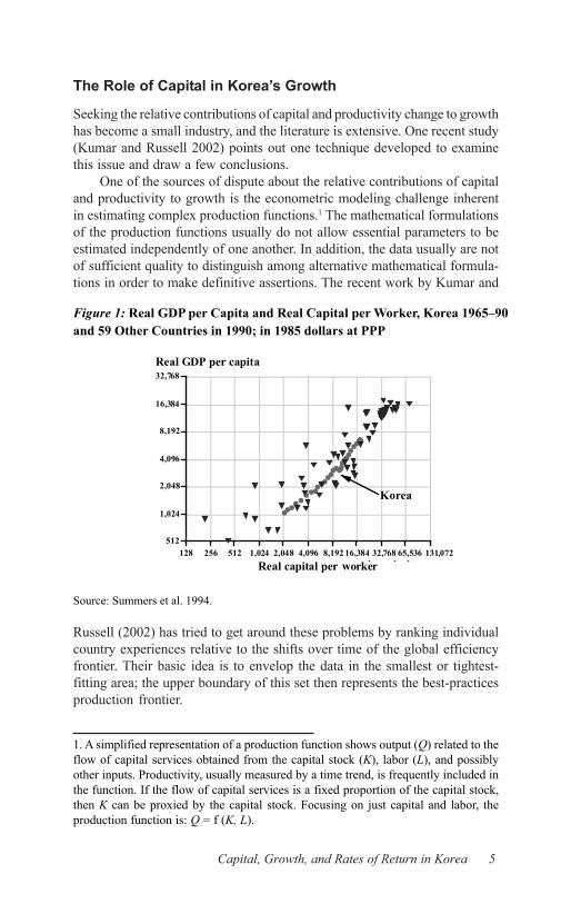
Korea’s growth experience fits the standard theory. Figure 1 plots a 1990cross section for 59 countries of gross domestic product (GDP) per capitaagainst the amount of capital invested per worker. Also in Figure 1 is the timeseries data for Korea from 1965 to 1990. Korea’s experience falls right on thecurve of the other countries.

According to Figure 1, economic development certainly is associatedwith higher levels of capital, and Korea is marching along the same basicpath as the rest of the world’s economies. While some countries seem to getmore GDP per capita from the same amount of capital as employed by Korea,others get less. It is not possible from only these data to decide how wellKorea is using its resources, although it may be hard to argue against anyprocess that has enlarged real output per person by a factor of almost 10 in 25years.


The Role of Capital in Korea’s Growth

Seeking the relative contributions of capital and productivity change to growthhas become a small industry, and the literature is extensive. One recent study(Kumar and Russell 2002) points out one technique developed to examinethis issue and draw a few conclusions.

One of the sources of dispute about the relative contributions of capitaland productivity to growth is the econometric modeling challenge inherentin estimating complex production functions.1 The mathematical formulationsof the production functions usually do not allow essential parameters to beestimated independently of one another. In addition, the data usually are notof sufficient quality to distinguish among alternative mathematical formula-tions in order to make definitive assertions. The recent work by Kumar and

Russell (2002) has tried to get around these problems by ranking individualcountry experiences relative to the shifts over time of the global efficiencyfrontier. Their basic idea is to envelop the data in the smallest or tightest-fitting area; the upper boundary of this set then represents the best-practicesproduction frontier.

1. A simplified representation of a production function shows output (Q) related to theflow of capital services obtained from the capital stock (K), labor (L), and possiblyother inputs. Productivity, usually measured by a time trend, is frequently included inthe function. If the flow of capital services is a fixed proportion of the capital stock,then K can be proxied by the capital stock. Focusing on just capital and labor, theproduction function is: Q = f (K, L).

32,768

16,384

8,192

4,096

2,048

1,024

512

131,07265,53632,76816,3848,1924,0962,0481,024512256128

Real GDP per capita

Real capital per worker

Korea

Figure 1: Real GDP per Capita and Real Capital per Worker, Korea 1965–90

and 59 Other Countries in 1990; in 1985 dollars at PPP

Source: Summers et al. 1994.


0

10,0

00

20,0

00

30,0

00

40,0

00

50,0

00

60,0

00

70,0

00

80,0

000

5,000

10,000

15,000

20,000

25,000

30,000

35,000

40,000

Korea

JapanHongKong

1990 frontier

1965 frontier

GDP per worker

Capital per worker

Figure 2: World Production Frontiers, 1965 and 1990; and Growth Paths of

Korea, Japan, and Hong Kong, 1965–90, in 1985 dollars at purchasing power

parity


Their sample consists of 57 countries over the period 1965–90 and usesdata from the Penn World Table (PWT) version 5.6 (Summers et al. 1994).They look at real GDP per worker as a function of real nonresidential capitalstock per worker, and they construct production frontiers for 1965 and 1990.Figure 2 reproduces their frontiers, together with the 25-year experience ofthree countries: Korea, Japan, and Hong Kong.

One of the findings of Kumar and Russell is that the expansion of thefrontier is not neutral with respect to capital but instead strongly favors capi-tal-rich countries. This effect can be seen in Figure 2 as the 1990 frontiermoves outward at capital levels greater than $20,000 per worker (1985 prices)but inward at low levels of capital. The authors conjecture that this apparentbackward movement of technology may come from their assumption of con-stant returns, which may not be tenable for very poor countries, or a possiblynonexistent best practice among the group of poor countries. In other words,even the best of the very poor countries may not be operating at the availablelevels of best practice.

Japan’s growth as shown in Figure 2 was dominated by capital deepen-ing. Korea’s path was somewhat less efficient than Japan’s until the end ofthe 1980s, when Korea was able to generate more GDP than Japan from itscapital stock at the same capital-labor ratio. However, the star performer inthis analysis was Hong Kong. Although it was substantially below the fron-tier in 1965 (Hong Kong’s performance was slightly inferior to Korea’s at thestart of the period in Figure 2), Hong Kong became by 1990 one of the fron-tier economies and helped to define best practice.


Kumar and Russell (2002, 534) use an economy’s distance from thefrontier and its relative movement to separate the effects of productivity andcapital deepening. They decompose an individual country’s change of GDPper worker into three components:

• Change in efficiency, measured by the change in the vertical distancefrom the frontier between periods;

• Technology change—the vertical shift in the frontier itself; and• Effect of change in the capital-labor ratio—in other words, the move-

ment along the frontier.

The decomposition can be carried out along two paths that vary accord-ing to whether the first-period frontier or the second is the base for the calcu-lation. This decomposition is shown in Table 1 for Korea, Japan, Taiwan, andHong Kong; the table uses both 1965 and 1990 as base years. In separate dataappendices, Kumar and Russell report results based on different assumptionsabout scale economies; the results vary little for these countries.2

One can conclude from Table 1 that most of the growth of output inKorea, Taiwan, and Japan came from increasing the capital stock. Hong Kong,in contrast, moved onto the frontier; its growth of GDP per worker, whichwas even greater than Japan’s, depended relatively little on increasing capitalintensity. In fact, Kumar and Russell conclude that most worldwide produc-tivity improvement was attributable to capital accumulation. Moreover, itappears that countries that are already rich in capital have benefited morefrom technological progress than from investment. The anomalies includeJapan—which has achieved rich-country status but continues to grow by capi-tal accumulation—and Hong Kong—a relatively undeveloped country thathas grown by increasing its productivity rather than its capital. It remains tobe seen how Korea will evolve.

2. To produce the percentage change in output per worker from the contributing fac-tors, divide each number in the table by 100 and add 1.0. Then multiply these newchange factors together to obtain the change in output per worker.


Tabl

e 1:

Dec

ompo

sitio

n of

Out

put G

row

th p

er W

orke

r in

Kor

ea, J

apan

, Tai

wan

, and

Hon

g K

ong,

196

5 to

199

0

Cou

ntry

Cha

nge

in o

utpu

t

Con

trib

utio

n to

per

cent

age

chan

ge in

out

put p

er w

orke

r

p

er w

orke

r (%

)

1

965

base

yea

r

1

990

base

yea

r

C

hang

e in

Cha

nge

in

Cap

ital

Cha

nge

in

C

hang

e in

Cap

ital

effi

cien

cy

t

echn

olog

y

Dee

peni

ng

ef

ficie

ncy

tech

nolo

gy

de

epen

ing

(%)

(%

)

(%)

(%

)

(%

)

(%)

Kor

ea42

4.5

31.7

–6.9

297.

531

.713

.722

5.6

Japa

n20

8.5

2.5

31.5

127.

72.

50.

919

6.6

Taiw

an31

9.0

10.6

10.9

229.

110

.68.

323

7.0

Hon

g K

ong

251.

112

0.0

3.7

53.8

120.

01.

157

.9

Sour

ce: K

umar

and

Rus

sell

2002

, App

endi

x.

Estimating Aggregate Rates of Return 9

3Estimating Aggregate Rates of Return

Capital Elasticities and Share of Output

The method used here to estimate economy-wide rates of return makes use ofproduction functions, which describe outputs as a function of inputs.3 Theparticular objective of the use of this method is to obtain the change of out-put related to changes in capital, holding other inputs constant. For aggregateproduction functions, this quantity can be interpreted as the economy-widereal return to capital.

Used here, in particular, is a parameter often included explicitly in pro-duction functions: the elasticity of output with respect to capital. This elastic-ity is defined as the ratio of the percentage change in output attributable to apercentage change in capital. If we had an estimate of the elasticity, multiply-ing this estimate by the ratio of GDP to capital stock would result in theindicator sought: the change of output attributable to increased capital stock.

The job looks easy: get an estimate of the elasticity of output with re-spect to capital and multiply the estimate by the ratio of GDP to the capitalstock. Scores of studies on productivity growth use production functions astheir theoretical foundation; it would seem, therefore, that elasticity estimatesshould be readily available for the purposes here. For example, a review ofproductivity studies for Korea can be found in Sung (2000). However, notmany studies actually estimate this elasticity in fully articulated productionfunctions even though that concept motivates the analysis; the reason thateconomists have moved away from estimating production functions stems

3. If the production function is Q = f (K, L), where Q is output, K is capital, and L islabor, then the change of output related to changes in capital, holding other inputsconstant, is the partial differential of Q with respect to K, or MQ/MK. The elasticity ofoutput with respect to capital is e = (MQ/Q)/(MK/K). If we multiply this elasticity by theratio of output to capital, we get the desired partial differential of output with respectto capital: e (Q/K) = (MQ/Q)/(MK/K) Q/K =MQ/MK.


from their goal of separating the contributions of capital to income growthfrom the contributions of productivity to income growth. These calculationsare bound up with the particular functional form of the production functionassumed in the empirical estimation procedure. Identifying the separate con-tributions of capital and productivity often is not possible without makingexplicit assumptions about the key parameters of the production function,such as returns to scale or the elasticity of output with respect to capital.Therefore, it is often simpler to make these assumptions explicitly and usesimpler techniques to arrive at the desired productivity trends.4

If it is assumed that the production function has an elasticity of substitu-tion equal to 1.0, that inputs are paid their marginal product (an assumptionabout the competitiveness of factor markets), and that there are neither econo-mies nor diseconomies of scale, then the elasticity of output with respect tocapital is constant and equal to capital’s share of output. For elasticity ofsubstitution values less than 1.0, a situation thought to be the case for devel-oping countries, the share of capital in national income declines as capitalgrows relative to labor.

Rather than laboriously estimating production functions, for which—inany event—it is often impossible to pin down the essential parameters withany precision, many economists have taken the short cut of assuming valuesfor these parameters on the basis of their readings of the data. In their studyof productivity, for example, Collins and Bosworth (1996, 154–5) assumethat capital’s share of GDP is 0.35 for all 88 countries. Their review of theliterature suggests that the share tends toward constancy and is somewherebetween 0.3 and 0.4, perhaps somewhat higher in the fast-investing Asiancountries. They also note that some authors find the share to be declining ina subsample of the high-investment economies. However, they argue thatassigning the same value to all countries reduces the problems of measuringproductivity change across countries and that the assumption does not dogreat violence to their data. Nevertheless, if the several conditions necessaryto make the simplifying assumption that the labor share is equal to the elas-ticity of output with respect to capital are not true, the resulting estimates willbe incorrect.

4. Chang-Tai Hsieh (2000) shows how, with different assumptions about the elasticityof substitution, the same data can generate variations in the estimates of productivitychange. For example, Korea’s average annual growth rate of total factor productivitycomputes to 3.25 percent if the elasticity of substitution is 0.3, but only 1.31 percent ifthe elasticity of substitution is 1.3. The elasticity of substitution is a measure of theease with which inputs can be substituted for each other. If L is the flow of labor inputsand K represents the flow of capital services, the elasticity of substitution is the per-centage of change in K/L for a 1 percent change in MK/ML, while production is heldconstant. This measure can range from zero (no substitutability) to infinity (perfectsubstitutability).


In contrast, economists Jong-Il Kim and Lawrence Lau (1994) formallytest the simplifying production function assumptions for a group of advancedand developing Asian countries. They find that the assumptions can be re-jected: the elasticity of substitution is less than 1.0, returns to scale are di-minishing, and factors are not paid their marginal product. Their results showthat the elasticity of output with respect to capital declines with the capitalintensity of production.5 Therefore, because the elasticity of output with re-spect to capital falls rapidly with the accumulation of capital, rates of returncalculated with these Kim and Lau elasticities will demonstrate rapid de-clines from high initial levels.

A study by Nazrul Islam (1995, 1145 [Table 3]) was consistent with Kimand Lau (1994) in finding that capital elasticities are lower for richer coun-tries than for poorer countries. Islam combined time-series data for individualcountries with cross section information across 96 countries; his estimate ofthe capital elasticity for the entire group was around 0.44, whereas the valuefor the 22 developed OECD countries was a much lower 0.30. AlthoughIslam assumed a standard production function with a coefficient of substitu-tion equal to 1.0 and constant returns to scale, estimates for the separatesamples suggest that capital elasticity declines with capital intensity.

Several authors have assumed constant returns to scale and competitivefactor markets but find a falling capital share of output; this implies an elas-ticity of substitution less than 1.0. However, estimating capital shares is notwithout its own set of problems. A widely used strategy is estimating thelabor share of national income from the amount of employee compensationin GDP. The share going to capital is then taken to be the residual. The appar-ent stability of shares in the United States led Cobb and Douglas (1928) tocome up with their eponymous production function as one that would pre-serve a constant labor share regardless of changes in relative factor prices.Moreover, the apparent stability of shares in other advanced countries led tothe easy acceptance of the simplifying assumptions mentioned above.

As data on developing countries improved, however, international crosssections showed wide disparities in labor shares across countries (Gollin 2002).In particular, the labor share seemed to increase with real per capita GDP,although there is great dispersion among the poorer countries. Gollin andothers have pointed out that the main reason that labor shares apparently risewith income is because there is a larger fraction of self-employed in poorercountries; their compensation is incorporated in the national-income term“operating surplus” rather than under “employee compensation.” Severalactivities generate the incomes of these workers: entrepreneurial activities,

5. According to Kim and Lau (1994), the elasticity, e, of output with respect to capitaldecreases as K/Q increases—a result that comes from their finding that the elasticityof substitution is less than 1.0.


capital investments, and pure labor income. The analytical issue is to sepa-rate out the labor portion of their income. When such adjustments are made,labor shares across countries with real per capita GDP greater than $4,000 liewithin a narrow range of approximately 0.66. However, the considerablenumber of countries below this income threshold continues to exhibit a widerrange of outcomes (Gollin 2002, 472).

In principle, therefore, we have at least two approaches to obtaining theelasticity of output with respect to capital:

• Values obtained from full production function estimations, and• Capital share of national income, generally derived as the remainder

after the labor share has been estimated.

With the elasticity in hand, it is then possible to calculate the return tocapital.

For Korea (Figure 3), the plotted 1990 capital shares and elasticities, aswell as those not plotted, lie between 0.25 and 0.35. All the estimates thatallow for change over time show a declining trend.6

To make meaningful comparative statements about rates of returns, weneed some reference values. Finding that returns in Korea are, say, 13 percentreally tells us very little without some comparisons—comparisons, for ex-ample, with the cost of capital, with past returns, or with the values in othercountries that are at various stages of development. There is a problem, though,in comparing across studies: because each study uses its own equations, esti-mating methods, and data sources and definitions, meaningful comparisonsacross studies are problematic. Thus, if one study produces a value of the rateof return for Korea and a different study generates estimates for Japan, itwould be difficult to make other than gross comparative statements about the

6. While extending the Pilat (1994) estimates from 1990 to 2002, I discovered an errorin the original compilation. National income typically is divided into employee com-pensation and operating surplus. As mentioned, part of operating surplus can be at-tributed to the labor of family businesses and other owner-operated firms. To get a truelabor share, part of the operating surplus should be attributed to the labor input ofowner-operated businesses and the remainder to capital. Pilat imputed 50 percent ofthe average annual wage rate of wage and salary workers (for whom there is reporteddata) to the self-employed, and 25 percent to unpaid family workers. The sum of theselabor categories, plus a constant 5 percent attributed to land income, was tallied as thelabor share of national income at factor cost. Pilat, however, inadvertently used na-tional income at market prices instead of national income at factor costs. This mightseem to be a trivial point, of interest only to national income accountants, except thatit changes the capital share by a substantial 5 to 12 percentage points. In Figure 3, Iplot corrected and updated figures instead of the original figures; in addition, to makethe numbers comparable with the other estimates, I assumed only two factors of pro-duction and did not deduct a 5 percent payment to land.


two countries. One way to reduce many of the potential sources of incompa-rability and overcome this problem is to search for studies that include asample of several countries.

Kim and Lau (1994) estimated production functions for five developedcountries and four fast-growing Asian ones, including Korea. Their explicitpurpose was to compare the growth and productivity experiences of thesecountries. They make none of the simplifying assumptions typical in the lit-erature; instead they estimate the parameters of a fully specified productionfunction. They allow their elasticities to vary across countries and over timeto account for changing structures of production.

Measuring Capital Stock

Three approaches are commonly used to estimate the national stock of capital:

• Surveys of enterprises,• Perpetual inventory method that sums up past investment while continu-

ally depreciating each vintage of capital, and• Perpetual inventory method without depreciation that assumes stable out-

put until the life of the item expires.

Angus Maddison (1995) has favored the last method in his attempts tocreate standardized capital estimates for several countries. The PWT uses theperpetual inventory method with annual depreciation.

0.1

0.2

0.3

0.4

0.5

0.6

Young

Singh

Kim and Lau

Pilat/Alexander

200019951990198519801975197019651960

Elasticity or share

Figure 3: Alternative Elasticities or Capital Shares, Korea, 1960–2002

Sources: Kim and Lau 1994; Pilat 1994, Annex Table 1.7; Singh 1998, 132; Young 1995, 660.Note: Used

here are Kim and Lau elasticities and capital share estimates by Pilat, Singh, and Young. The results by Pilat

(1994) have been corrected by the author; see footnote 6. Two other estimates are not shown in this figure

because they did not vary over time: Collins and Bosworth (1997) assumed a constant value of 0.35 for their

entire sample over all years, and Gollin (2002) calculated an adjusted share for many countries, including

Korea, for a single year. Gollin’s 1991 value for Korea is 0.303.


The survey method can produce inconsistent estimates because of in-complete coverage and problems encountered in answering complex ques-tionnaires (Timmer and van Ark 2002). Pyo (1998, 39–40 [Table 10]), usingsurveys in benchmark years and a perpetual inventory method for intercensusperiods, has constructed capital stock estimates for Korea. Discovering defi-ciencies in Korea’s earlier wealth surveys, Pyo adapted his estimation meth-ods to help overcome them. Pyo’s gross stock estimates, which remove in-vestments from the pool on the basis of assumed lifetimes of different classesof assets, are similar in spirit to Maddison’s. Net capital stock is calculatedby depreciating the gross figures; Pyo estimated depreciation rates by calcu-lating the pattern of depreciation that would make the surveys consistent withintercensus investment.

Maddison constructed standardized estimates of capital stock for sev-eral countries. He did not rely on data reported by national statistical organi-zations because he observed that official estimates of asset lives vary moreamong countries than seems legitimate. For example, asset lives for nonresi-dential structures vary from 39 years in the United States, to 57 years in Ger-many, to 66 years in the UK. National statistical authorities in neighboringFinland and Sweden assume an average service life of buildings in manufac-turing of 42 years and 70 years, respectively. Maddison (1995, 138) notes:“When countries, which, by world standards, are so similar have very differ-ent assumptions about virtually identical assets, it seems likely that there is asignificant element of incomparability.”

Maddison’s standardized estimates assume asset lives that approximateas closely as possible those in the United States: structures are given 39-yearlifetimes, and equipment is given 14 years. One of his findings from thestandardized capital stock figures for the United States, the UK, France, Ger-many, Netherlands, and Japan is that the ratio of nonresidential capital toGDP has not been stable over the long term and has varied among countries;this observation, he notes, contradicts the widely shared assumption that theratio has been steady in advanced economies.

It is particularly easy to calculate the capital stock according to theMaddison scheme: simply add up the real investment for the number of yearsthat correspond to the lives of the different asset classes. This measure of thegross stock of capital is the cumulative value of past investment still in exist-ence. The problem with this approach is that, to produce a stock estimate, itrequires a stream of data at least as lengthy as the longest-lived asset. Theother problem is that the productive quality of assets generally decays overtime, and this method does not take the deterioration into account. This defi-ciency is not an issue if investment is stable; but if it grows rapidly—as iscommon in fast-developing economies—the capital stock figure may bedistorted.

Timmer and van Ark adopted Maddison’s method in their estimates ofKorea’s and Taiwan’s capital stock. These authors performed sensitivity analy-


ses to test the implications of their choice of asset lives. For example, if,instead of their chosen lives of 39 years for structures and 14 years for equip-ment, the lifetimes were 30 and 10 years, the aggregate capital stock at theend of the period in 1997 would have been 9 percent smaller; if the assetswere longer lived than assumed—45 and 19 years—the stock of capital wouldbe 9 percent greater. They conclude that such variations in lifetimes have alimited effect on the absolute value of the capital stock and an even smallereffect on its growth rate (Timmer and van Ark 2002, 13 [Table 4]).

Timmer and van Ark (2002, 14) also estimate what they call the produc-tive capital stock. They apply an annual rate of depreciation to gross invest-ment; their effective rate of efficiency decay is 11.8 percent per year for equip-ment and 2.3 percent for nonresidential structures.

Used here are the Maddison capital estimates for the United States andJapan and the Timmer and van Ark capital stock figures for Korea, all up-dated to 2002 from recent national accounts data.7 The capital stock data areconverted to a real 1990 base. For comparison, I also use the PWT approachto measuring capital stock, based on continuous depreciation to test the sen-sitivity of the rate-of-return figures to different capital assumptions. The PWTcompilers in their 5.6 version use annual depreciation rates of 3.5 percent forstructures, 15 percent for machinery, and 24 percent for transportation equip-ment. In the data appendix to PWT 5.6 (Summers et al. 1994), the compilersnote:

The present capital stock estimates will tend to be considerablylower than alternative measures that use [Maddison’s] one-horse-shay measure of gross capital stock. The latter estimates willretain the full value of past investments in the capital stock forthe average service life of the asset. A rationale for this approachis that until it is scrapped a piece of equipment is contributingto production at a constant rate. In the approach we have used,the assumed contribution of equipment to production is muchless if it is 10 years old than if it is 5 years old. The measure wehave provided is much closer to the value of capital at any pointin time. Whatever the merits of alternative approaches, the usershould not be surprised if our capital per worker estimates areoften half those of alternative measures.

When the PWT method is applied, capital stock estimates are 50–60percent of the value compiled according to the Maddison method from thesame data. Consequently, rates of return computed from the PWT capitalfigures will be roughly twice as high as those from the Maddison figures.

7. Because of data revisions since Maddison’s original work, I updated the U.S. datafrom 1982.


Considered here are several estimates of Korea’s capital stock: Timmerand van Ark’s perpetual inventory figures with no depreciation; Timmer andvan Ark’s “productive” capital series based on a perpetual inventory methodwith annual depreciation; Pyo’s approach based on benchmark surveys filledin with annual investment in a perpetual inventory method, both gross (with-out depreciation) and net (with depreciation); and the PWT approach of per-petual inventory, with their annual rates of depreciation applied to updatedinvestment series. International comparisons will be performed with theMaddison-style nondepreciated figures and with PWT depreciation.

Figure 4 shows these various measures of the stock of nonresidentialcapital. The three net estimates based on annual rates of depreciation arerelatively similar to each other; the two gross figures are considerably largerthan the depreciated stocks as well as different from each other. Timmer andvan Ark note that Pyo’s gross figures appear to be too high and that the esti-mated depreciation parameters are often implausible, a situation that castsdoubt on the consistency of the various benchmarks. For the following Ko-rean returns, I use the Timmer and van Ark capital figures calculated with theMaddison lifetime assumptions, and my capital figures calculated with thePWT assumptions. It should be underlined that both series are based on thesame historical investment data.

Estimating Korean Returns

Figure 5 shows returns on economy-wide nonresidential capital; these arebased on Timmer and van Ark’s nondepreciated capital series, estimated ac-cording to the Maddison assumptions.8 For comparison, I use three elastici-ties or capital shares that span the sample described above: Kim and Lau’selasticity estimated from a production function, Collins and Bosworth’s con-stant capital share, and my adaptation of Pilat’s capital share. Although thereare differences in the results for the earlier years, the overall pattern of changeis quite similar. Moreover, the more recent years show strong convergence.To simplify the results even further, Kim and Lau’s elasticities are extendedto 2002 at the same value estimated for 1990, the last year of their sample;for comparison, I use my recalculated Pilat share because it represents thelower bound of share or elasticity estimates.

In Figure 6, using the two elasticities and the two capital series basedon Maddison and PWT depreciation assumptions, I plot four different rate-of-return series. In addition, a market-based, real rate of return calculated byHsieh (2002, 507) is included for comparison. Hsieh sought the returns of an

8. GDP data came from Korea’s national accounts and from those of Japan and theUnited States. Price level–adjusted time-series data of real GDP with different baseyears were converted to a standardized 1990 base.


asset whose price is correlated with the returns of the country’s capital stock.For Korea, he chose the unregulated curb market rate and deflated it with theaverage rate of asset price deflation.9

Several points can be drawn from these alternative renderings of Korea’sreal rate of return on aggregate capital:

• Returns have fallen sharply over the years as capital has accumulated un-der Korea’s high savings and investment regime; the declines range from35 to 55 percentage points;

• PWT depreciation assumptions, as expected, lead to lower levels of capi-tal and higher returns than do the Maddison fully-productive-life assump-tion;

• The rate of decline became less steep after 1980 and probably flattenedbetween 1998 and 2002; and

• Returns during the first and second decade following the end of the Ko-rean War were extraordinarily high, no matter how measured; the Kimand Lau elasticities produced the highest estimates, possibly because theirprocedure allowed the elasticity of substitution to be less than 1.0, whichmay have forced a high capital elasticity in the postwar days when muchcapital had been destroyed. Hsieh (2002, 503) summarizes:

9. Hsieh wanted to determine whether capital stock is being correctly measured; hefound that Korea’s investment data appear to be consistent with other evidence butthat Singapore’s national accounts significantly overstate the amount of investmentspending.

0

200,000

400,000

600,000

800,000

1,000,000

1,200,000

PWT

Timmer and

van Ark (productive)

Timmer and van Ark (perpetual)

Pyo (net)

Pyo (gross)

20001995199019851980197519701965

Billions of won

Solid lines –net estimates

Dashed lines –gross figures

Figure 4: Alternative Measures of Korea’s Nonresidential Capital Stock,

1965–2000, in billions of 1990 won

Sources: Pyo 1998, Summers et al. 1994, Timmer and van Ark 2002.


[T]here is overwhelming evidence that the marginal product of capitalhas fallen by the extent implied by the national accounts. All three measures[of the marginal product of capital in Korea] indicate that it has fallen dra-matically since the 1960s.

0.0

0.2

0.4

0.6

0.8

1.0

Pilat/Alexander

Collins and Bosworth

Kim and Lau

200019951990198519801975197019651960

Rate of return

Figure 5: Rates of Return on Nonresidential Capital, Korea, 1960–2002

Sources: Collins and Bosworth 1996, Kim and Lau 1994, Pilat 1994.Note: The results by

Pilat (1994) have been corrected by the author; see footnote 6.

0.0

0.2

0.4

0.6

0.8

1.0

1.2

Pilat, PWT

Pilat, Maddison

Hsieh

Kim and Lau, Maddison

Kim and Lau, PWT

200019951990198519801975197019651960

Rate of return

Figure 6: Rates of Return on Nonresidential Capital in Korea,

1960–2002

Sources: Hsieh 2002, Kim and Lau 1994, Maddison 1995, Pilat 1994, Summers et al.

1994.

Note: Maddison and PWT assumptions for depreciation; Kim and Lau and Pilat elasticities;

and Hsieh real returns based on curb rate.


A pattern similar to Korea’s very high postwar rates followed by steepdeclines was seen in Europe and Japan following World War II. The explana-tion for this is that these countries had preserved their human capital andinstitutions from the earlier period but lacked the capital that had been de-stroyed during the war. Consequently, the economies were in severe disequi-librium since the proportions of their productive inputs had been selectivelyaltered; when investment recovered, the returns to the new additions to capi-tal were very large. As the capital stock rose to equilibrium levels, however,returns declined to levels appropriate to the mix of human, physical, andinstitutional capacities. Because Korea had not been a rich country before theKorean War, it also benefited from starting from a particularly low level ofcapital and output.

Figure 7 zooms in on the portion of Figure 6 for the years after 1980;this will allow a clearer examination of the period when the decline in therate of return decelerated. Two main features stand out: returns remain high(8–16 percent) despite almost 50 years of fast-paced investment; and the down-ward trend may have been reversed following the reforms of the Asian finan-cial crisis.

In addition to the production function method of calculating returns,scholars have used the simpler ratio of output to capital (Q/K) that describesthe amount of capital in use in an economy in relation to the value of output;this ratio takes no account of other sources of output—it holds nothing elseconstant. In particular, the output-capital ratio does not tell how much moreoutput might be expected from an increase in the capital stock.

The ratio of the change of output to the change in the capital stock—theincremental output-capital ratio—is somewhat closer to the goal of attribut-ing marginal changes in output to marginal increases of capital. If capitalwere the only factor experiencing change, Q/ K would be sufficient; how-ever, this ratio does not account for other variables that also may be affectingoutput. Therefore, the preferred measure in this chapter—the partial differ-ential MQ/MK—yields theoretically more satisfying estimates of rates of re-turn. Figure 8 shows these three output-capital measures.

The three ratios paint the same qualitative picture: very high levels fol-lowing the recovery from wartime devastation in the early 1960s and subse-quent declines as capital-fueled economic development went into high gear.The large swings in Q/ K arise from the year-to-year cyclical fluctuationsin investment. Because the other measures are based on ratios of the annualflow of GDP to the stock of capital, neither of which changes by more than afew percentage points, the trends are considerably smoother.

International Comparisons

We can now compare the returns in Korea with returns in other countries.Returns for Japan and the United States were calculated with elasticities fromKim and Lau extended through 2002 plus capital stock figures based on both


the Maddison and PWT assumptions (shown in Figure 9). Japan, like Korea,earned high returns in the years after World War II. By the end of the period,however, Japan’s rates had fallen substantially below U.S. rates. In contrast,according to these estimates, Korea’s returns are still well above U.S. re-turns. Although the difference between Japan and the United States does not

0.00

0.05

0.10

0.15

0.20

0.25

0.30

0.35

Pilat, PWT

Pilat, Maddison

Hsieh

Kim and Lau,Maddison

Kim and Lau, PWT

20001995199019851980

Rate of return

Figure 7: Rates of Return on Nonresidential Capital in Korea,

1980–2002

Note: Maddison and PWT assumptions for depreciation; Kim and Lau and Pilat elasticities;

and Hsieh real returns based on curb rate.

Sources: Hsieh 2002, Kim and Lau 1994, Maddison 1995, Pilat 1994, Summers et al.

1994.

–1.5

–1.0

–0.5

0.0

0.5

1.0

1.5

2.0

Q/K

∆Q/∆K

∂Q/∂K

2000199519901985198019751970

Percentage

Figure 8: Alternative Measures of the Capital and Output Relationship, Korea,

1970–2002

Sources: Kim and Lau 1994, Maddison 1995.


seem to be very great at the scale of Figure 9, Japanese returns in 2001 were40 percent less than the U.S. estimate under both capital assumptions.

Returns in the United States have been relatively stable compared withthose in the other two countries, both of which experienced recovery fromwar followed by unprecedented investment-led growth. Nevertheless, U.S.returns of 15–20 percent in the 1950s were still high for the world’s mostadvanced economy. The United States had experienced a dearth of invest-ment because of the Great Depression that was followed by the diversion ofresources to the World War II effort. The accumulation of new technologyand the almost 20-year investment drought plus the revival of postwar de-mand generated high returns.

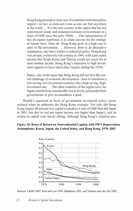
Figure 10 shows the same countries as shown in Figure 9 with the addi-tion of Hong Kong (C&SD 2003). What may be surprising is the consider-ably slower decline of returns in Hong Kong, which have been substantiallyabove returns in Korea.10 The main reason for Hong Kong’s high returns isthe relatively low level of investment that has been required to produce ahigh level of GDP per capita. In an attempt to explain this seemingly diver-gent experience, Rodrik (1997, 25–8) cites the absence of government in-tervention policies:

10. According to the original PWT 5.6 investment and capital figures (Summers et al.1994), returns actually increased in Hong Kong to the end of the data series in 1992.However, revised investment data recently published in Hong Kong are inconsistentwith the PWT 5.6 investment trends. I re-estimated the capital stock using the newdata, with the results shown in Figure 10.

0.0

0.1

0.2

0.3

0.4

0.5

0.6

0.7

0.8

0.9

1.0

200019901980197019601950

Dashed lines – Maddison assumptions

Solid lines – PWT assumptionsKorea

Japan

United States

Rate of return

Figure 9: Rates of Return on Nonresidential Capital, with Maddison and

PWT Assumptions; Korea, Japan, and the United States, 1950–2002

Sources: Kim and Lau 1994, Maddison 1995, and Timmer and van Ark 2002.


Hong Kong presents a clear case of a noninterventionist policyregime—in fact, as clear-cut a case as one can find anywherein the world. . . .It is the only country in the region that has notexperienced steady and sustained increases in investment as ashare of GDP since the early 1960s. . . .One interpretation ofthis divergent experience is to claim success for the strategyof laissez faire. After all, Hong Kong grew at a high rate inspite of flat investment. . . .However, there is an alternativeexplanation, one that is kinder to industrial policy. Hong Kongwas already a relatively rich country in 1960, with a per capitaincome that South Korea and Taiwan would not reach for atleast another decade. Hong Kong’s transition to high invest-ment appears to have taken place largely during the 1950s.

Hence, one could argue that Hong Kong did not face the cen-tral challenge of economic development—how to transform alow-saving, low-investment economy into a high-saving, high-investment one. . . .The other countries of the region (save forJapan) started from considerably lower levels, and needed theirgovernments to give accumulation a push.

Rodrik’s argument in favor of government investment policy seemsstrained when he addresses the Hong Kong example. Not only did HongKong require 40 percent less capital to produce a unit of GDP than did Japanin 2001, but also its real per capita income was higher than Japan’s, and itsreturns to capital were barely falling. Although Hong Kong’s situation may

0.0

0.1

0.2

0.3

0.4

0.5

0.6

0.7

0.8

Hong Kong

United States

Japan

Korea

2000199019801970

Rate of return

Figure 10: Rates of Return on Nonresidential Capital, with PWT Depreciation

Assumptions; Korea, Japan, the United States, and Hong Kong, 1970–2002

Sources: C&SD 2003, Kim and Lau 1994, Maddison 1995, and Timmer and van Ark 2002.


not be directly comparable with situations of larger countries, its experiencecannot be dismissed out of hand. High income, moderate investment, andhigh returns appear to be compatible outcomes.

Returns in Development Perspective

Are Korea’s earnings commensurate with its relative position as a still-developing economy, given the amount of capital that it has invested? Wecan portray Korea’s returns relative to its capital depth and compare its trendwith those of other countries. For such comparisons, capital stock per capita,rather than capital per worker, is a good measure of capital deepening be-cause different employment regimes can create variations in the participationrate that are independent of capital efficiency; normalizing capital stock bythe total population avoids such distortions.11

The analysis so far has been in terms of ratios of domestic currencies. Tocompare countries in a common currency, it is necessary to convert exchangerates. Because capital and GDP have been measured in 1990 values, all thatis required is 1990 purchasing power parity (PPP). Here, separate PPPs for GDPand investment are taken from PWT 6.1 (Heston et al. 2002) to convert into1990 dollars. The PPPs used to make the conversion are shown in Table 2.

The results for Korea, Japan, and the United States are in Figure 11; thetwo panels show the results when the capital stock is estimated according tothe Maddison and the PWT depreciation assumptions. The two approachesto estimating the capital stock produce almost identical qualitative results;the one difference, as seen earlier, is that returns with the PWT assumptionsare higher because the estimated quantity of capital is lower. Until the early1990s, Korea’s returns were slightly below Japan’s at the same level of capi-tal per person; Korea’s downward course flattened in the 1990s, and by around1994 its returns for a given level of capital surpassed Japan’s experience of30 years earlier. Japan’s returns, in turn, have been a bit below the U.S. valueat almost all levels of capital stock per person, with the gap growing in recentyears. Korea is following Japan’s example of a high-capital country; its 2002value of capital per capita surpassed the U.S. value of only 10–15 years earlier.

The similarity of Korea’s investment-led development path to Japan’spath is apparent in the ratio of GDP per capita as a function of capital stockper capita (Figure 12). The first thing to note in Figure 12 is that Korea’sexpansion path overlays Japan’s. The second thing is that U.S. growth afterthe early 1950s jumped to a new, productivity-based economic model. Theseresults indicate that Korea has used more capital than the United States toproduce each unit of GDP at comparable levels of capital intensity, or, alter-

11. Calculations using capital stock and GDP per worker show that U.S. productivityis considerably greater than both Korea’s and Japan’s, and that Japan’s is greater thanKorea’s (see Figure 14 on page 27).


natively, that Korea has generated less output per unit of capital. Neverthe-less, Korea earns higher returns on capital when estimated by the productionfunction approach. The difference must come from those other things thatare being held constant in the latter method.

Table 2: Exchange Rates and PPPs for Korea and Japan, 1990

Country Exchange rate (U.S. $) GDP PPP Investment PPPKorea 707.8 474.2 467.1Japan 144.8 183.9 166.5

Source: Heston et al. 2002.

The other things influencing capital returns are mainly high labor in-puts. McKinsey and Company (MGI 1998) has studied Korean productivityat the macroeconomic and industry levels, and its study compares Korea withJapan and the United States. One of its central analytical methods relateslabor and capital inputs to productivity to arrive at GDP per capita, as shownin Table 3. The table shows that Korea’s economy in the 1993–95 period hadinvested only 47 percent as much capital per capita as the United States, butit used 40 percent more labor in producing GDP. Korean capital productivitywas estimated to be 5 percent greater than the U.S. value, but labor produc-tivity was only 36 percent as great.

Baily and Zitzewitz (1998, 256–7) used the McKinsey study to generateadditional analysis. When they turned their attention to disaggregated manu-facturing and service sectors, they found capital productivity in Korean ser-vices to be 50 percent greater than in the United States and manufacturing

Table 3: Factor Inputs, Productivity, and GDP in Korea and Japan, 1993–95

Factor inputs Korea JapanCapital per capita 47 135Labor per capita 140 120Total factor inputs per capita 98 126ProductivityCapital productivity 105 60Labor productivity 36 70Total factor productivity 51 63GDPGDP per capita 50 80

Source: MGI 1998.Note: Labor and capital aggregated according to a Cobb-Douglas production function,with labor share of 66 percent. Korea and Japan indexed to U.S. 1993–95 average = 100.


capital productivity to be 20 percent below the U.S. level. They attributed thehigher returns in services to the fact that services had been starved of capitalunder Korea’s state-led industrialization process, whereas manufacturing re-ceived subsidized capital injections.

Indeed, according to Baily and Zitzewitz, industrial companies in Koreadid not earn enough on their capital to pay their cost of funds. Moreover,

0 20,000 40,000 60,000 80,000 100,0000.0

0.1

0.2

0.3

0.4

0.5

0.6

0.7

0.8

0.9

Korea

Japan

UnitedStates

Rate of return

Nonresidential capital (Maddison) per capita (1990 dollars at PPP)

0 10,000 20,000 30,000 40,000 50,000 60,0000.0

0.1

0.2

0.3

0.4

0.5

0.6

0.7

0.8

0.9

1.0

Nonresidential capital (PWT) per capita (1990 dollars at PPP)

Rate of return

KoreaUnitedStates

Japan

U.S. Dollars

Figure 11: Rates of Return and Capital Stock per Capita, with Alternative

Depreciation Assumptions; Korea, Japan, and the United States, 1950–2002

Sources: Maddison 1995; Summers et al. 1994.

U.S. Dollars


estimated corporate returns in the United States were considerably higherthan returns in Korea.

The inability of manufacturing companies to earn their cost of capital issupported by another study that looked at productivity in Korea’s economy.Park and Kwon (1995, 342) found that throughout the 1980s the price ofcapital in heavy industry was greater than its marginal product; light industry,in contrast, more than made its capital costs.

Baily and Zitzewitz (1998, 254) summarize their macroeconomic con-clusions by plotting per capita GDP as a function of labor and nonresidentialcapital, combined according to a Cobb-Douglas production function with a la-bor share of 66 percent. They compare Korea with long term-series data for theUnited States, Japan, France, and Germany. Their chart is reproduced as Figure13, in which both GDP and factor inputs are indexed to the 1995 U.S. values.

The central point of both the McKinsey study and the Baily and Zitzewitzstudy is that, by 1995, Korea and Japan had reached or exceeded the levels ofinputs of the other economies, but on a flatter, lower productivity path. Korea’sGDP per capita of about 50 percent of the United States in 1995 was achievedwith about the same level of inputs, albeit with a very different mix—morelabor and less capital. (Baily and Zitzewitz 1998, 254)

Baily and Zitzewitz conclude that the United States, Germany, and Francefollowed a productivity-oriented growth path, with much higher levels ofoutput at each level of input than the two Asian economies.

0 20,000 40,000 60,000 80,000 100,0000

5,000

10,000

15,000

20,000

25,000

30,000

Japan

Korea

United States

GDP per capita

Nonresidential (Maddison) capital per capita

Figure 12: GDP per Capita versus Capital Stock per Capita; Korea, Japan,

and the United States, 1950–2002, 1990 dollars at PPP

Sources: Maddison 1995, Timmer and van Ark 2002.


These points are buttressed by a comparison of the plots of GDP perworker against capital per worker with the similar plots of per capita ratios ofFigure 12. Because of high U.S. productivity in the use of labor, both theKorea and Japan curves of Figure 14 are considerably below the U.S. curve;the output produced by a unit of combined capital and labor is much greaterin the United States than in the other two countries.

Figure 13: GDP and Combined Inputs per Capita; Korea, United States,

Japan, Germany, France, various years ending 1995; U.S. 1995 = 100

Source: Baily and Zitzewitz 1998, 255 (Figure 2).

0

5,00

0

10,0

00

15,0

00

20,0

00

25,0

00

30,0

00

35,0

00

40,0

000

5,000

10,000

15,000

20,000

25,000

30,000

35,000

40,000United States

Japan

Korea

Real GDP per worker

Real nonresidential capital stock per worker

Figure 14: PWT 5.6 GDP per Worker versus Capital Stock per Worker;

Korea, Japan, United States, 1965–90, 1985 dollars at PPP



Japan has yet to make the transition from an input-dependent growthpath to one that relies on productivity. Korea is following in Japan’s foot-steps but is not as advanced as Japan. Korea is still earning returns greaterthan the other countries considered here. Its future path, however, remainsuncertain.

Rates of Return in Korean Corporations 29

4Rates of Return in Korean

Corporations

Because the financial accounts of many Korean companies sometimes dis-guise grim financial realities, the use of company figures in any analysis isopen to question. Two responses to this legitimate concern may serve to re-duce reasonable objections to the methods used here,12 although they cannotultimately guarantee unqualified support of the conclusions. First, this paperreports averages and medians of hundreds of companies rather than the fig-ures for any single one. Unless phony reports were the rule across most com-panies and unless these manufactured numbers grossly distort the underlyingreality in a nonrandom way, the results shown here should still be valid. Sec-ond, this paper provides statistical tests of differences between chaebol-re-lated and non-chaebol-related companies.

The large business groups of industrial and financial firms, called chaeboland often in the past controlled by a family founder, have been notable forthe problems revealed in the wake of Korea’s severe business contraction in1997 and 1998. If financial reporting errors reside mainly in large chaebolgroups, as presumed by many scholars on Korea’s economy, direct compari-sons of the two groups of companies may identify real issues. The analysis

12. For this paper, data on fiscal year (FY) 1997 through FY 2001 rates of return forKorean corporations came from the Korea Information Service (KIS 2002), whichprovides financial information of all companies listed on the Korea Stock Exchangeas reported to Korea’s Financial Supervisory Service. I selected for analysis all nonfi-nancial companies with reported profit and assets. The number of companies variedfrom year to year—from 458 companies in FY 1997 to 491 companies in FY 2001.Fiscal year can vary from company to company. To assign a fiscal year to a calendaryear for analytical purposes, I set the calendar year equal to the fiscal year if the fiscalyear ended in the second half of the calendar year; otherwise I set the fiscal year to theprevious year. Thus, if the fiscal year ended on 31 July 2001, I assigned it to calendaryear 2001; if it ended on 30 April 2001, I placed it in calendar year 2000.


that I describe at the end of this chapter did not uncover any obvious prob-lems. Of course, if all types of companies are guilty of misreporting, suchtests will not reveal it.

One other potential source of financial reporting errors must be consid-ered. The data analyzed in this and the next chapter are only for non financialfirms. If chaebol hide debt or off-balance sheet obligations in the financialaffiliates belonging to the group, they would not be on the books of the com-panies that I investigate. Close scrutiny of companies that have gone intobankruptcy such as Daewoo have tended to find more liabilities than hadbeen reported on the balance sheet. Until we get consistent and reliable con-solidated financial reporting that include financial and nonfinancial groupaccounts, the results obtained here will have to be considered as tentative.13

Measuring Profit

The first issue in estimating returns is the selection of a particular definitionof profit from among the several alternatives in the data: operating income;ordinary income; net income before taxes; and net income after taxes. Therelationship among these measures is shown in Table 4.

Operating income represents profit generated in a company’s main lineof business; it fits the standard notion of profit as equaling revenues minusproduction costs. Ordinary income includes nonoperating income and ex-penses that are unrelated to the main line of business. For example, it in-cludes gains and losses on currency transactions. Net income before taxesadds in extraordinary, one-time transactions. Finally, net income after taxessubtracts the company’s income tax liabilities.

To calculate returns, I used operating income and net income after taxes.Operating income is recorded after depreciation but before payments andreceipts of interest and dividends. A central assumption about an ongoingestablishment is that profit represents a payment to capital. If depreciationwere not deducted from the income stream, it would be equivalent to gener-ating income by selling the capital stock.

Another reason I used operating income is that it is recorded before thepayment of interest. Because the income generated by the capital stock iscentral to this study, the cost of a large part of that capital should not bededucted prematurely in the analysis. This consideration is especially impor-tant in Korea, where interest on borrowing is a major element of the cost ofcapital.

Net income after taxes is the income available to one particular class ofcapital providers: shareholders. This measure of income is what is left afterpaying off everyone else—the government, providers of current inputs such

13. This issue was pointed out by Edward M. Graham in a review of an earlier draft.


Table 4: Relation among Items in Income Statements of 491 KoreanCompanies, 2001, in billions of won

Total Income statement items483,950 Sales400,178 Costs of sales

83,770 Gross profit or loss56,970 Selling and administrative expenses

SalariesRetirement allowanceOther employee benefitsUtilitiesTaxes and duesRent

24,169 DepreciationEntertainmentAdvertisingOrdinary R&D expensesInsuranceTransport, handling, warehousing, packingBad debt expenseAmortization of intangible assetsAmortization of development costsOther selling & administrative expenses

26,798 Operating income or loss22,280 Nonoperating income

Interest incomeDividend incomeGain on foreign currency transactionsGain on foreign currency translationGain on valuation of marketable securitiesGain on disposition of tangible assetsOther nonoperating income

41,123 Nonoperating expenseInterest expenseLoss on foreign currency transactionsLoss on foreign currency translationLoss on valuation of marketable securitiesLoss on disposition of tangible assetsOther nonoperating expenses

7,956 Ordinary income or loss4,228 Extraordinary gain1,430 Extraordinary losses

10,755 Net income or loss before income tax expenses5,675 Income tax expenses5,078 Net income or loss after income tax

Source: KIS 2002.Note: The items in the table that show accompanying monetary amounts are available asdata for individual companies.


as labor and materials, and other suppliers of capital such as banks. Net in-come after taxes will be used to measure the returns to shareholder equity.

Table 5 gives the mean and median of the various profit indicators. Thereason for considering the median (the middle value in a distribution, aboveand below which lie an equal number of observations) is the great range ofcompany sizes, from the giant chaebol to their small suppliers. Outliers, par-ticularly very large firms, distort averages as measured by the mean and maycamouflage changes among the large number of smaller companies.

Table 5: Alternative Definitions of Korean Corporate Profit, 1997–2001, inbillions of won

Year No. of firms Operating Ordinary Net income Net income income income before taxes after taxes Mean1997 458 56.6 5.0 5.0 1.41998 481 46.6 4.9 –6.1 –11.61999 482 55.3 42.1 42.9 29.92000 487 74.9 33.4 31.8 17.52001 491 54.6 16.2 21.9 10.3

Median1997 8.3 2.8 2.8 2.01998 8.1 3.0 3.2 2.31999 8.6 6.4 7.1 5.12000 9.2 4.9 5.2 3.82001 8.8 5.1 5.2 4.0

Source: KIS 2002.

The first thing to notice about Table 5 is the large differences betweenmean and median. The median is much smaller and exhibits less variationover time. For example, the order-of-magnitude increase in the mean valueof ordinary income from 1998 to 1999 is subdued in the median. These dif-ferences suggest that ordinary averages may hide more than they reveal. Itwill be instructive, therefore, to examine more extensive representations ofthe distributions rather than to focus on any single number.

Measuring Assets

Just as there are alternative definitions of profit, assets also may be describedin several ways. The most inclusive measure is total assets, which incorpo-rates financial assets, inventories, and fixed assets such as plant and equip-ment. Because all of these assets enter the production of goods and servicesand because payments to these assets must be generated by profit, I use total


Table 6: Relation among Items on Balance Sheets of 491 Korean Companies,2001, in billions of won

Total Balance sheet items134,703 Current assets102,654 Quick assets

13,276 Cash and cash equivalents3,920 Marketable securities

46,540 Trade receivablesOther quick assets

32,048 InventoriesFinished or semifinished goodsRaw materialsOther inventories

Noncurrent assets124,294 Investments

Investment securities219,957 Tangible assets

LandBuildings and structuresMachinery and equipmentShips, vehicles and transportation equip.Construction in progressOther tangible assets

8,906 Intangible assetsDevelopment costs

488,192 Total assets149,657 Current liabilities

38,316 Trade payables32,677 Short-term borrowings from banks32,625 Current maturities of long-term borrowings

Current maturities of bonds payableOther short-term borrowingsOther current liabilities

Long-term liabilities62,487 Bonds payable24,825 Long-term borrowings from banks

Other long-term borrowingsLiability provisionsOther long-term liabilities

267,997 Total liabilities220,192 Stockholders’ equity

50,454 Capital stock103,490 Capital surplus

62,977 Retained earnings3,253 Capital adjustment

Source: KIS 2002.


assets as the denominator of the rate-of-return ratio; operating income is thenumerator. Shareholder equity will be used in the calculation of returns toshareholders.

Macroeconomic measures of economy-wide returns typically use thecapital stock of plant and equipment in their measurements, as I did in Chap-ters 2 and 3. These aggregations of physical capital omit the financial assetsthat I include when measuring private returns. In the balance sheets of Ko-rean companies, investment in plant and equipment is represented by tan-gible assets, which are only 45 percent of total assets. The relation among thevarious items of the balance sheet is shown in Table 6.

Why not use physical capital instead of the more inclusive total assets tocalculate company returns? The main reason is that a firm is not a country. Ifa corporation cannot repay its lenders and shareholders, its long-term sur-vival is doubtful. However, if all balance sheets were consolidated in an eco-nomic system without cross-border capital flows, the financial entries wouldcancel out because the assets on one balance sheet would be matched byliabilities on others. After netting, aggregate national nonfinancial invest-ments would remain on one side of the balance sheet and the nation’s savingson the other.

Table 7 presents means and medians of selected balance sheet items. Aswith income, outliers dominate the means, which are approximately five tosix times greater than the medians. Over the five years from 1997 through2001, median liabilities have fallen, equity has risen, and assets have grown.These trends mark the cleaning up of corporate balance sheets as companiestook steps to reduce their borrowing from previously dangerous levels.

Table 7: Selected Balance Sheet Items of Korean Companies, 1997–2001

Year Total assets Total liabilities Shareholder equity Leveragea

won, billions won, billions won, billions Mean 1997 877.9 663.0 214.8 3.03 1998 886.8 621.1 265.6 1.98 1999 1,021.4 583.5 437.9 5.80 2000 1,063.1 634.1 429.0 2.18 2001 994.3 545.8 448.5 2.24 Median 1997 144.0 95.4 49.0 2.06 1998 155.2 89.6 58.9 1.46 1999 175.3 89.9 75.9 1.10 2000 186.6 93.4 80.9 1.10 2001 183.2 84.4 83.5 1.02Source: KIS 2002.a. Ratio of total liabilities to shareholder equity.


Table 7 also shows Korean corporations’ average leverage, defined asthe ratio of total liabilities to shareholder equity. Because of outliers, themean ratio of liabilities to equity does not show a clear trend. The medianvalue, however, has fallen steadily in the past five years, and in 2001 it washalf its 1997 value. Highly leveraged financing (bank loans that were insuf-ficiently backed by equity capital) was one of the leading causes of Korea’seconomic crisis in 1997–98.

Average Rates of Return

Now that we have selected measures of profit and capital, we can calculaterates of return for Korean companies for 1997 through 2001. Table 8 pre-sents nominal returns on total assets and shareholder equity.

Table 8: Nominal Rates of Return on Total Assets and Shareholder Equity ofKorean Companies, 1997–2001

Year No. of Aggregate Aggregate Mean Median Median corpora- operating net income operating operating income tions income to after tax to income to income to after tax to to total shareholder total assets total assets shareholder assets equity (%) (%) equity (%) (%) (%)

1997 458 6.4 0.7 5.5 5.7 3.4 1998 481 5.3 –4.4 4.1 5.4 4.0 1999 482 5.4 6.8 4.9 5.2 6.3 2000 487 7.0 4.1 5.4 5.2 5.1 2001 491 5.5 2.3 4.7 4.9 4.6

Source: KIS 2002.

There are several ways to measure average returns. In Table 8 and Table9 (on page 36), the first measure is the sum of operating income divided bythe sum of total assets (column 3). This simple ratio is equivalent to theweighted mean across the observations where the weights are the proportionof each company’s assets to the sum total. The same ratio is calculated for netincome after tax to shareholder equity (column 4).

The next average (column 5) is the mean of all company returns. Be-cause the mean treats each company equally, small companies with extremevalues can produce distortions. Medians are shown next to the mean (column6); as mentioned earlier, outliers do not affect the median.

The mean value of the return on equity is so dominated by outliers that itis not even shown in the table. The reason for the extreme variability is thatequity capital was wiped out for a significant number of Korean companiesin the aftermath of the Asian financial crisis in 1997–98 and the subsequent


collapse of the Korean won. Consequently, in many cases, equity was veryclose to zero on both the positive and negative sides; a denominator near zerocauses very large positive and negative ratios. For example, the return onequity in 1999 ranged from minus 161,000 percent to a positive 1,720 per-cent; including such values in a mean so distorts the result that it would notbe meaningful to include it. Instead, I used the median figures (column 7).

Is there evidence in Korea’s corporate data of any trend, or signs, thatcorporate reforms have helped to push up returns? Nominal operating in-come to total assets (column 3, Table 8) shows a downward trend over thefive years. Although the evidence for a negative slope is weak, it is supportedby the regression equation at the end of the chapter in which other variablesare accounted for.

Shareholders’ returns (column 4, Table 8) have been particularly erratic.Net income after taxes tends to be more volatile than operating income. Ex-traordinary losses and gains unassociated with a company’s main line of busi-ness can be particularly large in severe downturns as capital losses and otherfinancial reverses overwhelm ordinary profit. Thus, aggregate losses in 1998—when the full effects of the Asian crisis were felt—were followed by a sharprecovery the next year. The difference in returns on shareholder equity be-tween those two years amounted to more than 10 percentage points. How-ever, the median company—the company in the middle of the pack—showedmuch less volatility.

Another approach to assessing the possibility of trends is to examinewhat happened to individual companies. I separately created a matched set of457 companies that existed in both 1997 and 2001. The median change ofreturns to total assets was negative: –0.4 percent. On the other hand, themedian return to shareholder equity rose by 0.7 percentage points. The same

Table 9: Real Rates of Return on Total Assets and Shareholder Equity ofKorean Companies, 1997–2001

Year Inflation, Aggregate Aggregate Mean Median Median GDP operating net income operating operating income deflator income to after tax to income to income to after tax to (%) aggregate shareholder total total shareholder assets equity assets assets equity

(%) (%) (%) (%) (%)

1997 3.2 3.2 –2.5 2.3 2.6 0.2 1998 5.0 0.3 –9.4 –1.0 0.4 –1.0 1999 –2.0 7.4 8.8 6.9 7.2 8.3 2000 –1.1 8.1 5.2 6.5 6.3 6.2 2001 1.3 4.2 1.0 3.5 3.6 3.3

Source: KIS 2002.


mixed pattern can be seen in aggregate, rather than median, returns. On anindividual company basis, there was no clear sign of improved returns in 2001.

If corporate returns are adjusted by the inflation rate of the GDP deflator(Table 9) it shows that 1999–2001 are better by all the measures than 1997.Falling prices in 1998 and 1999 pushed up real returns in those two years,and low inflation in 2001 helped to continue making real returns a bit betterthan in the years of faster price increases.

How do returns in Korean corporations compare with those earned else-where? It is a difficult question to answer because corporate financial report-ing is not standardized across countries; even within a country, financial dataoften do not fit economic definitions.

Keeping these concerns in mind, I tried to generate figures for the UnitedStates and Japan that may be compared with figures for Korea.14 The com-parisons are shown in Table 10. All the figures are based on ratios of aggre-gate profit to aggregate assets. The main difference across the country com-parisons is that Korea’s data are based on companies listed on the major

Table 10: Corporate Rates of Return in Korea, Japan, and the United States,1990–2001

Year Korea: Japan: Japan: U.S.: operating operating operating operating income to income to surplus to income to total assets total assets total assets total assets (KIS) (MOF) (ESRI) (IRS)

(%) (%) (%) (%) 1990 4.9 3.6 6.9 1991 4.5 3.7 1992 3.5 3.6 1993 2.9 3.4 1994 2.9 3.0 1995 3.0 3.2 7.1 1996 3.2 3.4 7.1 1997 6.4 3.2 3.5 7.1 1998 5.3 2.4 3.2 4.6 1999 5.4 2.8 3.0 4.3 2000 7.0 3.4 3.0 3.6 2001 5.5 2.9 2.8Sources: IRS 2001, KIS 2002, MOF 2002, ESRI 2002.

14. Japanese data came from two sources: MOF (2002) and ESRI (2002). Because theoperating surplus in the Japanese data includes some labor income, the calculatedreturns are too high. U.S. data are from IRS (2001); changes in U.S. definitions in1998 mark a break in the data.


national stock exchange, whereas the Japanese and U.S. observations includeall private, nonfinancial corporations.

Both the U.S. and Korean returns tend to be higher than the Japanesereturns. Whether measured by the MOF (2002) or ESRI (2002), returns inJapan have been declining since before the 1990s; even at the height of thebubble in 1990, they were lower than returns in Korea after the Asian finan-cial crisis. Although it is difficult to make fine comparisons, returns to Ko-rean companies are roughly comparable with returns in the United States.

The Distribution of Returns and Leverage

One question often raised about Korea’s economy is whether large size con-fers competitive or profitability advantage. The distribution of returns acrossan extremely wide range of asset sizes suggests that there is no simple rela-tion between size and profitability. Figure 15 shows a scatterplot of returns(operating income to total assets) versus total assets (on a logarithmic scale)for 2001. (Other years exhibit the same results.) The simple correlation be-tween returns and assets is 0.03; with the log of assets, it is 0.15. These cor-relations are evidence of no relationship. The correlation between leverageand assets is even lower: –0.004, which is about as random a relationship ascan be found. The regressions reported later suggest that the link betweenoperating profitability and assets is slightly positive but insignificant, andthat returns on equity are negatively, weakly, and insignificantly related toshareholder equity.

1000000100000100001000100

30

20

10

0

-10

-20

Total assets

Return on assets (%)

(billion won)

Figure 15: Ratio of Operating Profit to Total Assets versus Total Assets for 491

Korean Companies, 2001

Source: KIS 2002.


Another conjecture is that companies borrowed to finance profitableopportunities that could not be funded by the underdeveloped and overregu-lated Korean capital market. If so, there should be a positive relation betweenleverage and returns. This supposition is not supported by the data; the corre-lation between leverage and the return on total assets was –0.07 for 2001.

Another theory was that, by leveraging their investments, shareholderscould enhance their own returns by adding borrowed funds to their investedcapital. Again, this conjecture comes up short; the correlation between lever-age and return on shareholder equity is significantly negative: –0.46. Thisresult, however, is dominated by some extreme observations on returns,which—as noted above—can be very large or very small because of nearzero values of equity. If the influence of outliers is suppressed by the removalof the 50 most extreme variables, the correlation falls, but to a still signifi-cant –0.22 for the remaining 450 firms. Taking the logs of both variablesdrops the correlation of the remaining 410 positive observations to an insig-nificant –0.07.

If leverage declined so noticeably, why did profit not increase to thesame degree? After all, lower leverage means that borrowing (as a share oftotal funding) and its attendant interest costs must have declined. However,the first definition of returns—operating income to total assets—is calcu-lated before interest payments; therefore, a change in debt and interest pay-ments would not affect this measure of returns. The reason that returns onequity did not improve is that equity finance increased at about the same rateas profit. Moreover, although interest expense did fall by a percentage pointor two as a proportion of sales, the industry data indicate that interest costsare only about 3 to 5 percent of total costs (see Chapter 5). Other items suchas materials and personnel have a much greater impact on profitability.

One way to visualize a distribution of observations in compact form isby plotting the interquartile range between the 25th and 75th percentiles,along with the median at the 50th percentile. This shows the center of thedistribution along with a measure of its spread. The usual method of focusingon standard deviations is less useful in the situation here because of the verylarge outliers that distort the distributions’ properties. Under the conditionshere, percentiles are more meaningful.

Figure 16 shows the median and interquartile range of the rate of returnas measured by the ratio of operating income to total assets. The additionalinformation provided by the interquartile range is that it seems to have broad-ened and fallen slightly. The 25th percentile in 2001 is the lowest of the fiveyears, and the 75th percentile is tied for the lowest value. However, as notedabove, these differences are neither stark nor deeply informative of majortransformations in Korean companies.

Figure 17 shows the same kind of information about leverage. Here, thestory is more dramatic and more obvious. All parts of the distribution haveshifted downward, and the range is quite a bit narrower. The median value of


leverage fell by half as Korean firms reduced their borrowing and increasedtheir equity capital. An additional indicator of the sharp reduction in leverageis the interquartile range. In 1997, these values were 1.2 and 3.8; by 2001,they had fallen to 0.6 and 1.8. In other words, a financially conservativecompany in 1997 at the 25th percentile had higher leverage than the mediancompany five years later. By 2001, leverage in 75 percent of Korean compa-nies was less than 2.0, a substantial improvement over their precrisis balancesheets.

0

2

4

6

8

10

20012000199919981997

♦ ♦ ♦ ♦ ♦ Median

25th percentile

75th percentile

Percentage

Figure 16: Median and Interquartile Range of Returns to Total Assets,

1997–2001

Source: KIS 2002.

0

1

2

3

4

20012000199919981997

♦

♦♦ ♦ ♦

75th percentile

25th percentile

Median

Figure 17: Median and Interquartile Range of Leverage, 1997–2001

Source: KIS 2002.


Classification by Returns and Leverage

Another way to look at trends is to add a measure of financial leverage to thecomparisons of returns. Robert Feldman (2003), chief economist of MorganStanley Japan, has classified Japanese companies into four categories, de-pending on their combination of profitability and leverage. Feldman’s defini-tion of leverage is the same as that used here: the ratio of total liabilities toshareholder equity. Leverage acts as an indicator of the relative balance be-tween borrowed capital and equity capital. A high proportion of borrowedfunds makes a company particularly vulnerable to economic downturns whenthe mandated interest payments may not be adequately covered by profit.Feldman’s definition of returns also is the same as that used here: operatingincome to total assets.

Feldman’s four categories are based on a company’s position relative toaverage returns and average leverage: companies with above average profitand low leverage are defined as “winners,” low profit and low leverage are“plodders,” high leverage and high profit are “daring,” and low profit withhigh leverage are “losers.” I used the median values for the entire period toclassify companies: 5.3 percent return on assets and 1.3 for leverage, as shownin Table 11.

Table 11: Classification of Korean Companies by Profitability and Leverage,1997–2001, percentage of total number of firms

Year Winner Plodder Daring Loser1997 13.5 13.8 40.4 32.31998 24.3 20.8 27.0 27.91999 30.1 29.5 18.9 21.62000 28.7 30.2 20.5 20.52001 29.5 30.6 17.7 22.2

Sorce: KIS 2002.

When leverage is combined with rate of return during 1997–2001, aclear pattern emerges. The percentage of winners more than doubles and thepercentage of losers declines by one-third. This trend is dominated by therevolution in the balance sheet, which shows up in the fact that the share ofplodders (low returns, but also low leverage) more than doubles.

This classification reveals that Korean companies seem to have beenpaying more attention to reducing their risks from overreliance on borrow-ing than to increasing the return on their total capital base. Indeed, the gainshave been remarkable; and they parallel the course taken by Japanese com-panies, which have cut their leverage in half in the past 20 years (leverage atJapanese firms remains at a still dangerous 2.75, considerably higher than in


Korea). The next stage of corporate evolution could be higher returns througha combination of cautious investment and cost cutting to achieve greater ef-ficiency and improved productivity. That possibility remains in the future,however.

Testing the Difference between Chaebol and Non-ChaebolCompanies

Concern that the analysis of Korean firms may be colored by systematicmisreporting of financial information, especially by companies associatedwith the large chaebol, led me to test this proposition. I divided the sample ofcompanies into two subsamples, depending on chaebol membership. A com-pany was assigned to the chaebol group if it identified itself as belonging toone of the top 20 chaebol as reported in the April 2003 Korea Fair TradeCommission list of business groups by asset size. In addition, I placed a com-pany in the chaebol subsample if its main shareholder was a top-20 chaebolmember. In 2001, 64 companies met these criteria. See Table 12 for the dif-ferences between the median values of selected characteristics for chaeboland non-chaebol listed companies. Use of the first and last years in the totalsample (1997 and 2001) detected changes over time.

Chaebol companies are roughly 10 times larger than non-chaebol com-panies in terms of assets and sales; however, there was little difference be-

Table 12: Median Value of Financial Variables for Chaebol and Non-ChaebolListed Korean Companies, 1997 and 2001

Financial item 1997 2001 Chaebol Non-chaebol Chaebol Non-chaebol

Total assets (won, billions) 147.2 12.1 160.4 14.6Liabilities (won, billions) 116.8 7.6 107.6 7.0Shareholder equity(won, billions) 28.6 4.3 56.0 7.2Sales (won, billions) 101.0 10.4 160.7 12.8Largest shareholder (%) 18.5 20.1 19.2 20.1Operating income/totalassets (%) 5.9 5.7 6.1 4.5Operating income/shareholder equity (%) 2.3 3.6 4.5 4.6Leverage (ratio of liabilitiesto equity) 5.9 5.7 1.7 0.9Number of firms 63 395 64 427

Source: KIS 2002.Note: Firm is defined as chaebol member if it identified itself as belonging to one ofthe top 20 chaebol or if its main shareholder was one of the top 20. See text.


tween the two groups when it came to the holdings of their largest singleshareholder: about 20 percent of company shares were held by a single entity.

If the books were being manipulated, one might expect profit to be par-ticularly high or leverage low. Rate of return as measured by operating in-come to total assets was slightly higher among chaebol companies in 1997,and this increased in 2001; but non-chaebol returns on assets fell over theyears. Returns to equity, however, moved differently; they were higher fornon-chaebol companies in both years, but the chaebol members showed fastergrowth. Leverage was very high for both groups in 1997, but slightly higheramong chaebol firms; it fell dramatically over the next five years, especiallyin the non-chaebol sample.

These data do not raise any alarm bells about inaccurate reporting. Toinvestigate further, I performed statistical regression analyses on rates of re-turn and leverage to detect differences that may be obscured when calcula-tions do not control for characteristics such as firm size. The results are re-ported in Table 13. Explanatory variables include the year of the data, rang-ing from 1997 to 2001, the logarithm of total assets, the percentage of afirm’s shares held by its major shareholder, the year the firm was established,and a dummy variable equal to 1 if the firm is a member of a top 20 chaebolgroup and zero otherwise.

The statistics indicate that being owned by another firm had a statisti-cally significant and sizable effect on profitability; as ownership increasedfrom, say, 10 percent to 20 percent, returns on total assets would rise by 0.2

Table 13: Coefficients from Regression Analysis of Financial Results forChaebol and Non-Chaebol Firms, 1997–2001

Dependent Year Log total Shares Member Year Inter- R2

variable assets held by of top est. cept adjusted (100 major 20

million share- chaebol won) holder (%)Operating –0.23 0.10 0.02 0.34 0.036 393 0.011 income/ (2.5) (0.9) (2.0) (0.8) (3.0)total assets (%)Net income –0.08 –0.18 0.05 –0.78 0.110 –52 0.017 after (0.4) (0.7) (2.2) (0.8) (4.7)taxes/equity (%)Leverage –0.29 0.27 0.006 0.28 –0.004 587 0.132

(11.5) (8.8) (2.0) (2.3) (1.5)

Note: Number of cases = 1,964; t statistics in parentheses.


percentage points. Membership in a top-20 chaebol would raise returns onassets by 0.3 percentage points but cause a 0.8 percentage point fall in re-turns to equity, neither effect being statistically significant. It is interestingthat profitability increases for newer firms; returns on equity would be 1percentage point higher for a firm that is 10 years younger than another firms.Leverage rises modestly with chaebol membership and by very modestamounts with the percentage of shares held by a major owner. In short, thisanalysis of chaebol and non-chaebol firms does not reveal any suspiciousdifference in profitability or leverage that could be explained by accountingchicanery.

Rates of Return in Korean Nonfinancial Industries 45

5Rates of Return in Korean

Nonfinancial Industries

Data and Definitions

The main source of data on Korean industries is the Bank of Korea (BOK2002), which draws its sample from the National Tax Service file of corpora-tions required to file a tax report. Industries are defined in accordance withthe Korea Standard Industry Classification (SIC). The sample includes 37,024corporations selected from the 1998 National Tax Service file of 168,803corporations. The survey excludes several categories of corporations, includ-ing financial companies, nonprofit corporations, households, and small com-panies with sales of less than 2.0 billion won. All companies with annualsales of more than 70 billion won or that rank in the top five in their industryin terms of sales are included automatically. Other corporations in the surveyare chosen by stratified random sampling.

The BOK Internet site (www.bok.or.kr/svc/frame_eng.html) included datafor the years 1990 to 2001 for 42 industries. Because of changes in industrydefinition and coverage, the number of industries varies by year. The onlinedata include only certain financial and operating ratios, but linking severalratios made it possible to produce the same rates of return as used in thecompany analysis. More detailed data also are available at the BOK site, butdata are provided for the most recent three years only. The sample industriesare shown in Table 14.

Rates of Return

Table 15 shows average nominal returns across industries in Korea for theyears 1990 to 2001. The range of values that was so much a problem in thecorporate data is greatly reduced in the industry sample because an industrycomprises many firms, which averages out extremes. The Bank of Koreacalculated industry figures from which the returns in Table 15 were estimated


Table 14: Industries in Korea by SIC Code: Assets, Sales, and Average Ratesof Return on Total Assets

Code Name of industry 2001 assets 2001 sales Average return (won, (won, on total assets

billions) billions) 1990–2001 (%)B Fishing 1,333 1,158 3.4C Mining and quarrying 3,765 1,704 –4.5D15 Food products and

beverages 36,516 37,317 6.4D17 Textiles 34,810 32,813 4.5D18 Sewn wearing apparel and

fur articles 11,204 15,030 5.6D19 Leather, luggage and

footwear 4,361 7,226 5.6D20 Wood and products of wood

and cork, except furniture 2,628 3,059 5.6D21 Pulp, paper and paper

products 13,613 11,555 6.4D22 Publishing, printing and

reproduction of recordedmedia 8,481 8,637 4.8

D23 Coke, refined petroleumproducts and nuclear fuel 32,178 43,904 6.4

D24 Chemicals and chemicalproducts 60,536 52,183 7.6

D25 Rubber and plastic products 12,858 12,454 6.7D26 Nonmetallic mineral

products 25,069 19,011 6.4D27 Basic metals 52,640 42,215 5.9D28 Fabricated metal products,

except machinery andequipment 13,309 14,043 5.7

D29 Other machinery andequipment 21,567 19,692 6.3

D30 Computers and officemachinery 10,925 11,357 6.6

D31 Electrical machinery andapparatuses, not elsewhereclassified 12,804 13,109 6.5

D32 Electronic components, radio,TV, communicationequipment 88,764 13,065 10.9

D33 Medical, precision andoptical instruments, watchesand clocks 5,239 4,349 6.1

D34 Motor vehicles, trailers andsemitrailers 62,372 71,912 4.3

D35 Other transport equipment 28,303 1,773 6.1D36 Furniture and manufacturing,

not elsewhere classified 5,512 6,390 5.1continued


as the ratio of aggregates instead of as the average of individual firm ratios;this procedure tends to reduce the influence of outliers. Nevertheless, even atthe industry level, the ratio of net income to shareholder equity exhibited awide range of values, largely because equity was wiped out for a significantnumber of firms as Korea’s economy collapsed in 1998. For the same reason,the mean value of leverage surged in those years. These effects can be seen inTable 15 in the differences between the mean and median values.

Because of the remaining influence of outliers, even in these aggregateddata, the median values provide a better view of underlying trends. The driftof median returns is downward. This direction may be due in part to theintroduction of market pricing of assets (so-called mark-to-market valuations),but it is also consistent with the sharp deceleration of nominal GDP growthand the slowdown of real GDP.

E40 Electricity, gas, steam and hotwater supply 76,348 26,534 5.1

F Construction 87,266 96,567 2.7G50 Sale of motor vehicles, retail

sale of automotive fuel 6,381 10,523 2.8G51 Wholesale trade and

commission trade 77,237 213,604 4.0G52 Retail trade except motor

vehicles 29,881 39,818 3.9H551 Accommodation 13,894 4,037 2.8I60 Land transport except railways 7,618 10,091 3.2I61 Water transport 21,607 19,273 5.6I62 Air transport 14,758 7,967 3.4I63 Auxiliary transport activities

and travel agencies 5,198 6,000 5.9J642 Telecommunications 55,117 30,413 6.2L Real estate and renting and

leasing 5,677 2,149 2.5M72 Computer and related activities 11,065 13,679 5.7M74 Professional, scientific and

technical services 8,230 11,360 7.5M75 Business support services 2,631 4,075 6.9Q Recreational, cultural and

sporting activities 12,270 5,682 5.1Q87 Motion picture, broadcasting

and performing arts 4,307 3,416 8.9Q88 Other recreational, cultural

and sporting activities 7,963 2,266 2.7R90 Sewage and refuse disposal,

sanitation and similar activities 745 815 6.9

Source: BOK 2002.

Code Name of industry 2001 assets 2001 sales Average return (won, (won, on total assets

billions) billions) 1990–2001 (%)


Tabl

e 15

: GD

P G

row

th, R

ates

of R

etur

n, a

nd L

ever

age

in K

orea

n In

dust

ries

, 199

0–20

01

Yea

r

Gro

wth

rat

e,

Gro

wth

rat

e,

N

o. o

f

O

pera

ting

N

et in

com

e

Lev

erag

e

Ope

ratin

g

Net

inco

me

Le

vera

ge n

omin

al

rea

l GD

P

in

dust

ries

i

ncom

e to

afte

r ta

x to

in

com

e to

afte

r ta

x to

G

DP

(%)

(

%)

tot

al a

sset

s

shar

ehol

der

tota

l ass

ets

sh

areh

olde

r

(

%)

eq

uity

(%)

(

%)

e

quity

(%)

M

ean

M

edia

n19

9020

.69.

034

6.0

4.8

5.2

6.5

7.2

3.5

1991

21.1

9.2

345.

74.

64.

76.

16.

73.

719

9213

.55.

434

5.3

0.1

5.6

5.2

3.0

3.9

1993

12.9

5.5

345.

30.

85.

15.

94.

93.

619

9416

.58.

334

5.9

7.9

4.7

6.1

6.4

3.3

1995

16.7

8.9

355.

97.

14.

25.

87.

63.

419

9610

.96.

835

4.8

1.1

4.7

5.5

3.0

3.7

1997

8.3

5.0

355.

0–1

5.7

6.9

5.5

–4.6

4.5

1998

–2.0

–6.7

404.

4–1

8.3

9.7

4.7

–2.8

2.7

1999

8.6

10.9

404.

4–7

.73.

24.

95.

22.

020

008.

19.

342

5.7

–0.9

2.6

5.8

3.9

1.7

2001

4.4

3.0

425.

11.

52.

35.

84.

41.

5

Sour

ce: B

OK

200

2.


The 1998 profitability plunge was not fully balanced by increases insubsequent years. The trends can be seen more clearly in percentile charts.Figure 18 shows the interquartile range and medians for operating profit tototal assets. The widening of the distribution in 1998 persisted in the follow-ing years, implying that slower economic growth introduced a wider range ofoutcomes among Korean industries, mainly by punishing losers more harshlythan in the earlier years of fast growth. Industries performing at the 75thpercentile of returns are at about the same level during the latter half of theperiod as during the first half, whereas the 25th percentile industries are sub-stantially below the earlier values. The widening of outcomes was not appar-ent in the shorter time span for data that we had for corporations.

Real returns have moved up since 1990, in contrast with the downwardtrend of nominal returns (see Table 16). The driver behind the upward drift ofreal returns has been the decelerating pace of inflation; slowly falling nomi-nal returns were converted into rising real returns as annual inflation fellfrom almost 11 percent in the early 1990s to low or negative rates by the endof the decade. Again, because of outliers, median figures give the best senseof the overall movement in Table 16.

The conversion of nominal to real rates reveals that the apparently healthynominal returns of the precrisis period were somewhat of a mirage. For thefirst half of the 1990s, Korean companies were not earning enough to com-pensate for rising prices (as measured by the GDP deflator). Ironically, slower

2

3

4

5

6

7

8

9

2001

2000

1999

1998

1997

1996

1995

1994

1993

1992

1991

1990

♦

25th percentile

75th percentile

Median

Percentage

♦

♦♦ ♦ ♦

♦ ♦♦ ♦

♦ ♦

Source: BOK 2002.

Figure 18: Interquartile Range and Median of Operating Income to Total

Assets, by Industry, 1990–2001


growth and milder inflation have yielded higher real returns, which show upeven for shareholders, who are doing better in real terms in the postcrisisperiod than they did in the earlier days when stock prices were rising faster.

Table 16: Real Rates of Return on Total Assets and Shareholder Equity forKorean Industries, 1990–2001

Year Inflation rate, Mean Median Mean net Median net GDP operating operating income after income after deflator (%) income to income to tax to tax to total assets total assets shareholder shareholder (%) (%) equity (%) equity (%) 1990 10.8 –4.8 –4.3 –6.0 –3.6 1991 10.8 –5.1 –4.7 –6.2 –4.1 1992 7.7 –2.4 –2.5 –7.6 –4.7 1993 7.0 –1.7 –1.1 –6.2 –2.1 1994 7.6 –1.7 –1.5 0.3 –1.2 1995 7.2 –1.3 –1.4 –0.1 0.4 1996 3.9 0.9 1.6 –2.8 –0.9 1997 3.2 1.8 2.3 –18.9 –7.8 1998 5.0 –0.6 –0.3 –23.3 –7.8 1999 –2.0 6.4 6.9 –5.7 7.2 2000 –1.1 6.8 6.9 0.2 5.0 2001 1.3 3.8 4.5 0.2 3.1

Source: BOK 2002.

This trend in real rates shows up clearly in Figure 19, which plots realreturns over time. Except for the collapse of shareholder returns in 1997 and1998, the trend over the period has been solidly positive. Even the slowdownbeginning in 2001 was not enough to return the figures to earlier levels.

In Table 17, the annual percentage change of the GDP deflator is sub-tracted from the U.S. and Japanese returns shown in Table 10. Comparisonsamong Korea, Japan, and the United States of real returns suggest that Ko-rean companies in 2001 were generating higher earnings than their counter-parts in the other two countries. Even in Japan, when deflation is added tothat country’s miserable nominal returns, the bottom line begins to look morecompetitive. Although these international comparisons can only be acceptedas suggestive, Korean companies do seem to have improved their real returnsmarkedly over the past decade; whether this has been the accidental sideeffect of more moderate price gains or a result of changes in corporate policyand governance remains unanswered.


Table 17: Real Nonfinancial Industry Rates of Returns in Korea, Japan, andthe United States, 1990–2001

Year Korea: Japan: Japan: U.S.: median operating operating operating operating income to surplus to income to income to total assets total assets total assets total assets (MOF) (ESRI) (IRS) (KIS) (%) (%) (%) (%)1990 –4.3 2.5 1.2 3.31991 –4.7 1.6 0.8 —1992 –2.5 1.8 1.7 —1993 –1.1 2.3 2.4 —1994 –1.5 2.8 2.9 —1995 –1.4 3.4 3.6 5.21996 1.6 4.0 4.1 5.21997 2.3 2.8 2.7 5.91998 –0.3 2.5 3.0 3.21999 6.9 4.2 4.3 2.22000 6.9 5.4 4.9 1.22001 4.5 4.3 — —

Sources: IRS 2001, KIS 2002, MOF 2002, ESRI 2002.

–8

– 6

– 4

–2

0

2

4

6

8

2001

2000

1999

1998

1997

1996

1995

1994

1993

1992

1991

1990

Median real net income

to shareholder equity

Median real operating

income to total assets

Percentage

Figure 19: Real Rates of Return in Korean Industries, 1999–2001

Source: BOK 2002.


Winners and Losers

Are there industries whose returns consistently have appeared at the top orbottom of the league standings? Table 18 lists the number of times an indus-try appeared in the annual rankings of the five best and five worst performers(defined as the ratio of operating income to total assets). Two traditional in-dustries—mining and fishing—were among the poorest performers. Out of apossible 12 appearances among the worst five, mining made it every year; infact it was at the bottom of the list 10 times and never had positive returnsover the entire 12 years. One possible explanation is that the mining sectorrequires high capital investment and has been plagued by falling commodityprices. The fisheries business has been affected by sharply falling yields asfishing grounds worldwide have been depleted. Other traditional industries—including leather and footwear, textiles, apparel, and construction—tend tomake up much of the rest of the list of the worst-performing industries.

Table 18: Lowest- and Highest-Performing Industries in Korea, 1990–2001

Lowest-performing No. of times Highest-performing No. of times industries on annual list industries on annual list

Mining 12 Electronics 11Fishing 6 Chemicals 7Motor vehicle sales 6 Computers 6Real estate 5 Professional andAir transport 4 technical services 4Computers 3 Computer services 3Land transport minus Movies, TV, theater 3 railroads 3 Nonmetallic products 3Motor vehicles 3 Precision instruments 3Computer services 2 Telecommunications 3Leather and footwear 2 Other transport equipment 3Publishing, printing 2 Paper and paper products 2Recreation, culture 2 Rubber, plastic 2Retail, excluding autos 2 Wearing apparel 2Textiles 2 Basic metals 1Construction 1 Electric machinery, other 1Fabricated metal products 1 Fabricated metal products 1Petroleum, etc. 1 Fishing 1Precision instruments 1 Leather and footwear 1Wearing apparel 1 Other machinery andWholesale trade 1 equipment 1

Petroleum, etc. 1Transport support, etc. 1

Source: Compiled from data at BOK 2002.Note: Performance is defined as ratio of operating income to total assets.


In contrast, the advanced technological industries of electronics, chemi-cals, and computers have been perennial occupants at the top of the leaguestandings since 1990. In addition, technical services and entertainment gen-erated high returns, reflecting the growth of services and the rise of newconsumer products. Because of the electronics sector’s cycles of technologyand demand, however, computers, computer services, and precision instru-ments as well as electronics also appeared among the worst performers sev-eral times. The average return for electronics (industry D32 in Table 14) overthe 12 years was 10.9 percent.

One of the major changes in financial structure has been the decline ofleverage among Korean companies. Because the corporate data went backonly to 1997, it was not possible to see longer trends. However, industryleverage figures reveal that the downward trend really did not begin until 1998,following the financial devastation imposed on overleveraged companies.

This point is clarified in Figure 20, which shows the interquartile rangefor the 12-year period. Leverage actually climbed in 1997 on the eve of thefinancial crisis. It then fell very rapidly, and the dispersion among industriesshrank. A telling point is that the 75th percentile in 2001 had an averagevalue of leverage below the 25th percentile as recently as 1998; moreover,the 2001 median was less than the lowest figure 10 years earlier.

We can classify whole industries by profitability and leverage in thesame way that was done for companies in Chapter 4. Recall that industrieswith above-average profit and low leverage are classified as winners; high-leverage and high-profit industries are daring; low profit and low leveragedefine plodders; and low-profit industries with high leverage are losers. With

0

1

2

3

4

5

6

2001

2000

1999

1998

1997

1996

1995

1994

1993

1992

1991

1990

25th percentile

Median

75th percentile

♦

Minimum

♦♦

♦

♦

♦♦♦♦♦♦♦

Figure 20: Median and Interquartile Range of Leverage for Korean

Industries, 1990–2001

Source: BOK 2002.


the same 1997–2001 average values for classifying industries as were ap-plied in Chapter 4—5.3 percent return on assets and 1.3 for leverage—therewere no winners in Korea until 1999, when leverage fell low enough to turnhigh-return industries into long-run bets (Table 19). The influence of highleverage in the classification can be seen in the column labeled Daring. Morethan 70 percent of the industries in 1990 had higher-than-average returns, buttheir leverage was high enough to make them risky, as events later in thedecade would prove. The numbers in the losers column peaked in 1998 butthen fell below the 1990 level.

Table 19: Classification of Korean Industries by Profitability and Leverage,1990–2001, percentage of annual total

Year Winner Plodder Daring Loser1990 0.0 0.0 70.6 29.41991 0.0 0.0 70.6 29.41992 0.0 0.0 44.1 55.91993 0.0 0.0 55.9 44.11994 0.0 2.9 67.6 29.41995 0.0 0.0 62.9 37.11996 0.0 0.0 54.3 45.71997 0.0 0.0 54.3 45.71998 0.0 2.5 40.0 57.51999 10.0 10.0 32.5 47.52000 9.5 14.3 42.9 33.32001 11.9 14.3 47.6 26.2

Source: Source: Compiled from data at BOK 2002.

Only a single industry fell into the winner category on Table 19 for thethree years for which there were winners (1999, 2000, and 2001): motionpictures, broadcasting, and performing arts. Business support services ap-peared in 2000 and 2001. No other industry appeared more than once.

Members of the daring category, home to almost half Korea’s industries,have the advantage of relatively high returns, but they still carry dangerouslevels of leverage. A brighter, and more secure, future lies ahead to the extentthat companies can shed their liabilities, build up their equity, and increasetheir profit.

It is instructive to compare Korea’s progress on returns and leveragewith Japan’s experience. Balance sheet reform in Japan has been similar toKorea’s but not as deep. Figure 21 shows the trend of return on assets versusleverage in both Korea and Japan since 1991. Nominal returns have fallen in


both places, and leverage has fallen significantly; Japanese companies, how-ever, still have dangerously high levels of debt on their collective balancesheets and have not progressed as aggressively as Korean companies in build-ing their equity and reducing their borrowing. This evidence suggests thatcompanies and national policies on restructuring have made greater progressin Korea than in the country from which they have borrowed so many of theirpast policies.

1 2 3 4 52

3

4

5

6

7

Leverage

Operating income tototal assets (%)

Korea

1990

2001

Japan

1990

2002

Figure 21: Rates of Return and Leverage in Korea and Japan, 1990–2002

Sources: Table 15 and MOF 2002.

Returns, Productivity, and Policy 57

6Returns, Productivity, and Policy

Productivity

Most economic growth studies examine productivity, not rates of return. Pro-ductivity can be defined simply as the ratio of outputs to inputs; total factorproductivity includes all inputs in the calculation. Although productivity andrate of return share several attributes, they do not always tell the same story.For example, countries can have very different average productivity levels,and yet companies in these countries can compete fiercely across borders.The balancing factor is exchange rates, which can convert a company in alow-productivity country into an international competitor.

Even within a country, industries and products with fast-growing pro-ductivity are not necessarily profitable; one need look only at the airline in-dustry in the United States or at semiconductor memory production almostanywhere to see two examples of the fastest-growing productivity and someof the worst profitability. In semiconductor DRAM memories, global pro-ductivity leader Micron has a 50 percent advantage over the average Korean,Japanese, and U.S. producer, but the company’s profitability has consistentlyunderperformed the U.S. market average. Within Korea, Samsung has thehighest productivity and is profitable at 85 percent of the Micron standard,whereas the less productive Hyundai and LG produce losses at 60 percentand 45 percent of Micron’s productivity, respectively (Baily and Zitzewitz1998, 265). However, profitability of companies within an industry in a spe-cific country will tend to be related to productivity. In the U.S. airline indus-try, Southwest Airlines is the most profitable and the most productive. Theimportant point is that companies do not take productivity to the bank; theytake their returns.

For Korea to join the ranks of the advanced European and North Ameri-can economies, it will have to shift to a productivity-based growth path fromits past reliance on mobilizing capital and labor. In particular, two problemsemerge from studies on Korea’s productivity: low labor efficiency andmisallocated investment.


The labor productivity issue arises especially in Korean manufactur-ing. Timmer and van Ark (2002, 21 [fig. 3]) note that in manufacturing thegap in labor productivity between Korea and Taiwan on the one hand andthe United States on the other is large. With the same amount of capital perhour worked, the United States generated approximately twice as muchoutput in the 1960s as Korea and Taiwan did at the end of the 1990s.

Noland and Pack (2002, 43) present evidence showing that the rate ofreturn to capital in the heavy and chemical industries—those favored byKorea’s industrial policy—were substantially lower than in light manufac-turing at the beginning of the high, forced-investment period of the early1970s. Noland and Pack contend that plowing more funds into a sector thatalready had low returns was a costly misallocation of capital.

Studies on Korean productivity are fairly consistent from one to the other.One finding is the collapse of productivity growth during the heavy- andchemical-industry promotion period from 1973 to 1981. Park and Kwon (1995)estimated that productivity change turned sharply negative during this periodas capital investment proceeded more rapidly than output. Timmer and vanArk (2002) also judged that productivity growth was a negative 0.4 percentannually during this period but that it turned to a positive 2.2 percent in 1985–96.

Park and Kwon find greater economies of scale in light industry than inheavy industry, suggesting that heavy industry has already exploited most ofits advantages because of its preferred investment situation. Timmer and vanArk support this conclusion with their evidence that labor productivity formanufacturing is substantially lower than for the total economy.

The McKinsey case studies (MGI 1998) support these macroeconomicconclusions by supplying explanatory details at the industry and companylevels. They found, for example, that automobile production companies inKorea invested in a capital intensity equal to that of the United States despitelower wage rates and higher interest rates. Another reason for low productiv-ity among Korea’s auto manufacturers is that the companies did not adopt theproductivity-enhancing lean production methods, pioneered in Japan andadopted worldwide. McKinsey experts estimated that the workforce couldhave been reduced by 15 percent without substantial reorganization and lossof output, but unions made layoffs of excess workers impossible and evenprevented reductions in hours. Managers were judged almost exclusively onoutput; consequently, defects were higher than in Japanese cars, and Koreancars sold for a 20 percent discount in the U.S. market, which had a severeeffect on profitability. Korean companies could have taken advantage of for-eign technology and techniques, but because of nationalism they did not linkwith foreign companies.

Why did these productivity-dulling practices exist in Korean auto pro-duction? The McKinsey analysts concluded that foreign competition wasdeliberately suppressed by high tariffs and barriers to foreign direct invest-

Returns, Productivity, and Policy 59

ment. Several nontariff barriers such as restrictions on foreign ownershipof distribution channels and government lists of foreign car owners keptownership of foreign cars to less than 1 percent of the market (MGI 1998,5–10).

Policy Issues

Baily and Zitzewitz conclude, as do many writers on Korea, by emphasizingthat most countries would be delighted to achieve Korea’s growth, savings,investment, education, and income. Nevertheless, why did it not achieve evenhigher productivity? They conclude that Korea transferred technology em-bodied in capital goods but not management practice. Capital was misallocatedowing to government policy influencing bank lending. Industrial policy wasoften rationalized by the assertion that immature and fragmented marketslack the capacity to make rational judgements because they cannot take intoaccount the feedback, network effects, and long-term consequences of in-vestments. However, Korean government policy did not make economicallyrational decisions. Partly this was due to moral hazard in finance; but equity,too, was put at risk. These were not gambles that went wrong; they would nothave earned enough to cover the cost of capital even if all the plans hadworked out (Baily and Zitzewitz 1998, 292).

These authors raise a critical question: Could Korea have grown as fastor faster if it had adopted a different development strategy? Korea followedthe Japanese path of input-driven growth—with long work hours, high sav-ings, channeled industrial investment, export orientation, limits on nones-sential investment and inward foreign direct investment, and restrictions onretailing. That path carried penalties for productivity. Noland and Pack try toanswer this question explicitly; they conclude that infant-industry arguments,potential gains from higher rates of return in preferred industries, and totalfactor productivity growth do not support the proposition that industrial policyworked or was essential to Korea’s growth. “The evidence does not supportthe notion that selective intervention had a decisive (or even necessarily apositive) impact on the Korean economy (Noland and Pack 2003, 44).”

Edward M. Graham at the Institute for International Economics goesfarther. His study concludes that the misallocation of capital, although creat-ing much economic benefit for the Korean people, also produced politicaldiscontent and excess capacity financed largely by debt (high leverage). Thisdangerous combination sowed the seeds of political instability and change inthe early 1990s and of bankruptcy, dissolution, and ongoing weakness amongthe leading chaebol later in the decade, both before and after the Asian eco-nomic crisis (Graham 2003, 79–87).

However, we do not know whether the long work hours and high sav-ings could have been mobilized in a more open and consumer-orientedeconomy. We do not know whether more foreign direct investment or im-


ports competing against infant industries would have encouraged greaterproductivity or would have led to industrial infanticide, or whether killingoff new industries might have been desirable.

The evidence from Hong Kong demonstrates that a high-productivity growth path is possible. Korean companies and workers havedemonstrated their ability to take advantage of new opportunities andproduce higher incomes for the hard-working, high-saving Korean people.In the coming years, if economic reforms continue, perhaps the Koreanpeople will realize even greater benefits from their sacrifices.

References 61

References

Baily, Martin Neil, and Eric Zitzewitz. 1998. “Extending the East Asian Miracle:Microeconomic Evidence from Korea.” Brookings Papers on EconomicActivity, Microeconomics.

Bank of Korea (BOK). 2002. Financial Statement Analysis. Seoul: BOK.

Census and Statistics Department (C&SD). 2003. Key Economic and Social In-dicators. Hong Kong: C&SD. March. www.info.gov.hk/censtatd/eng/hkstat/key_indicators/key_index.html.

Cobb, C. W., and P. H. Douglas. 1928. “A Theory of Production.” AmericanEconomic Review 18 (supplement):139–65.

Collins, Susan M., and Barry P. Bosworth. 1996. “Economic Growth in EastAsia: Accumulation versus Assimilation.” Brookings Papers on Eco-nomic Activity 2. www.brook.edu/dybdocroot/es/commentary/journals/bpea_macro/1996_2.htm#top.

Economic and Social Research Center (ESRI). 2002. Quarterly Estimates of GDP.Tokyo: ESRI. www.esri.cao.go.jp/en/sna/qe032/gdemenuea.html.

Feldman, Robert. 2003. “Japan: Keep Digging.” New York: Morgan Stanley, Glo-bal Economic Forum. 21 February. www.morganstanley.com/GEFdata/digests/20030221-fri.html.

Gollin, Douglas. 2002. “Getting Income Shares Right.” Journal of PoliticalEconomy 110:458–74.

Graham, Edward M. 2003. Reforming Korea’s Industrial Conglomerates. Wash-ington, D.C.: Institute for International Economics

Heston, Alan, Robert Summers, and Bettina Aten. 2002. Penn World Table, ver-sion 6.1. Philadelphia: Center for International Comparisons, Univer-sity of Pennsylvania. October. http://pwt.econ.upenn.edu/.

Hsieh, Chang-Tai. 2000. Measuring Biased Technology. Working paper, Depart-ment of Economics, Princeton University. www.wws.princeton.edu/~chsieh/DIVISIA4.pdf.

———. 2002. “What Explains the Industrial Revolution in East Asia? Evidencefrom the Factor Markets.” American Economic Review 92, no. 3 (June).

Internal Revenue Service (IRS). 2001. “Table 14b.--Corporation Income TaxReturns: Selected Balance Sheet, Income Statement, and Tax Items,by North American Industry Classification System (NAICS) IndustrialSector, Income Years 1998 - 2000.” Washington, D.C.: U.S. Depart-ment of the Treasury. www.irs.gov/pub/irs-soi/00co14b.xls.


Islam, Nazrul. 1995. “Growth Empirics: A Panel Data Approach.” Quarterly Jour-nal of Economics 110, no. 4 (November).

Kim, Jong-il, and Lawrence J. Lau. 1994. “The Sources of Economic Growth ofthe East Asian Newly Industrialized Countries.” Journal of the Japa-nese and International Economies 8, no. 3 (September): 235–71.

Korea Information Service (KIS). 2002. Korean Stock Market, Comapany Analysis.Seoul: KIS. www.kisinfo.com/KoreanStockMarket/index_ss.htm.

Kumar, Subodh, and R. Richard Russell. 2002. “Technological Change, Techno-logical Catch-up, and Capital Deepening: Relative Contributions toGrowth and Convergence.” American Economic Review 92, no. 3 (June).

Maddison, Angus. 1995. Standardised Estimates of Fixed Capital Stock: A Six-Country Comparison. In Explaining the Economic Performance ofNations: Essays in Time and Space, edited by Angus Maddison.Brookfield, Vt.: E. Elgar.

McKinsey Global Institute (MGI). 1998. Productivity-led Growth for Korea. Seoul,Washington, D.C.: MGI. March. www.mckinsey.com/knowledge/mgi/Korea.

Ministry of Finance (MOF). 2002. Financial Statements Statistics of Corpora-tions by Industry; Historical Data, Quarterly. Tokyo: MOF.www.mof.go.jp/english/e1c002.htm.

Noland, Marcus, and Howard Pack. 2003. Industrial Policy in an Era of Global-ization: Lessons from Asia. Washington, D.C.: Institute for Interna-tional Economics.

Park, Seung-rok, and Jene K. Kwon. 1995. “Rapid Economic Growth with In-creasing Returns to Scale and Little or no Productivity Growth.” Re-view of Economics and Statistics 77, no. 2 (May).

Pilat, Dirk. 1994. Economics of Rapid Growth: The Experience of Japan andKorea. Brookfield, Vt.: E. Elgar.

Pyo, Hak K. 1998. Estimates of Fixed Reproducible Tangible Assets in the Re-public of Korea, 1953–1996. Working Paper 9810. Korea Develop-ment Institute, Seoul. December.

Rodrik, Dani. 1997. TFPG Controversies: Institutions and Economic Performancein East Asia. Working paper 5914. National Bureau of EconomicResearch, Cambridge, Mass. February.

Singh, Ajit. 1998. “Savings, Investment and the Corporation in the East AsianMiracle.” Journal of Development Studies 34, no. 6:112–37.

References 63

Summers, Robert, Alan Heston, Daniel A. Nuxoll, and Bettina Aten. 1994. PennWorld Table, version 5.6. Cambridge, Mass.: National Bureau of Eco-nomic Research.

Sung, Yeung-kwack. 2000. “Total Factor Productivity Growth and the Sources ofGrowth in Korean Manufacturing Industries, 1971–1993.” Journal ofthe Korean Economy 1, no. 2 (Fall): 229–65.

Temple, Jonathan. 1999. “The New Growth Evidence.” Journal of Economic Lit-erature 37 (March).

Timmer, Marcel P., and Bart van Ark. 2002. Capital Formation and ProductivityGrowth in South Korea and Taiwan: Beating Diminishing Returnsthrough Realizing the Catch-Up Potential. Groningen, Netherlands:Groningen Growth and Development Centre, University of Groningen.March. www.econ.yale.edu/seminars/trade/tdw02/vanark-020408.pdf.

Triplett, Jack E. 1998. A Dictionary of Usage for Capital Measurement Issues.Paper presented at the second meeting of the Canberra Group on Capi-tal Stock Statistics, Organization for Economic Cooperation and De-velopment. 29 September–1 October. www.oecd.org/pdf/M00021000/M00021019.pdf.

Young, Alwyn. 1995. “The Tyranny of Numbers: Confronting the Statistical Re-alities of the East Asian Growth Experience.” Quarterly Journal ofEconomics 90, no. 3 (August): 641–80.

About the Author

Arthur Alexander is presently a consultant to industry and government cli-ents, and is a visiting professor at Georgetown University. He served as Presi-dent of the Japan Economic Institute in Washington, D.C. from 1990 to 2000.His professional experience also includes teaching positions at George Ma-son University and the Johns Hopkins University School of Advanced Inter-national Studies, and analytical positions at the Rand Corporation, the Inter-national Institute for Strategic Studies in London, and IBM. His publicationsinclude a book on the Japanese economy, In the Shadow of the Miracle, pub-lished in 2002 by Lexington Books. Dr. Alexander earned a Ph.D. in eco-nomics from the Johns Hopkins University in 1968.

Foreword

This study consists of five chapters. Chapter 1 is the introduction, and it covers the his-torical background of Korea’s economic growth, its export growth, and U.S.-Korea eco-nomic relations since 1950.

Chapter 2 first traces the evolution of Korea’s development strategies and phasesbeginning in the 1960s; it then describes the role of foreign investment and technology inthe growth of Korea’s economy. Chapter 2 concludes with a description and analysis ofKorea’s new development model, with its emphasis on science, the role of innovation,and the growth of service sectors.

Chapter 3 chronicles and analyzes Korea’s trade and investment patterns since 1960,including assessments of Korea’s growing position and competitiveness in world mar-kets. Separate sections address the special place of the United States in Korea’s traderelations and also Korea’s recent increasing involvement with Asian trade and invest-ment.

Chapter 4 deals with the impact of growing Asian regionalism over the past decadeand with the substantial increase in proposals and negotiations for bilateral, subregional,and regional trading arrangements among both Asian nations and nations outside Asia.This chapter also analyzes the results of various simulation models of the welfare andtrade impacts of proposed trade agreements; it uses proposed Korea-Japan and Korea-U.S. free trade agreements as key examples. It then explores the welfare effects on Koreaand the United States of a number of other proposed bilateral and regional trade arrange-ments.

Chapter 5 presents conclusions and recommendations for future U.S. and Korea traderelations on three levels: how to reconcile common and competing goals in the WorldTrade Organization Doha Round; potential responses and priorities of Asian and non-Asian countries regarding future bilateral, subregional, and regional trade agreements;and, after describing in some detail current bilateral disputes, Chapter 5 suggests a newframework for dealing with these issues.

Acknowledgments

I would like to thank Cordula Thum for her indispensable research and drafting supportthroughout the manuscript, Sung Woo-lim for his painstaking and thorough numberscrunching, and Andre Zlate for his work on the U.S.-Korea bilateral trade disputes. I amalso grateful for the thoughtful comments from three outside readers: Bernard Gordon,Nick Eberstadt, and Yang Jun-sok. Needless to say, any remaining errors in fact or inter-pretation are my responsibility.

Claude A. BarfieldAugust 2003

CORRIGENDUM

THIS CORRECTION APPLIES TO, Korea in Asia: Korea’s Development,Asian Regionalism, and U.S.-Korea Economic Relations, by Claude Barfield,Korea Economic Institute, 2003, Special Studies Series: 1.

In the Acknowledgments section of the Foreword, “Robert Gordon”should read “Bernard Gordon.” A corrected page is reproduced below.

KOREA’S CAPITAL INVESTMENT:RETURNS AT THE LEVEL OF THE ECONOMY,INDUSTRY, AND FIRM

Arthur Alexander

STUDIES SERIES: 2SPECIAL

KO

RE

A’SC

AP

ITAL

INV

ES

TME

NT

Arthur A

lexander

KOREA ECONOMIC INSTITUTE1201 F Street, NW, Suite 910

Washington, DC 20004Telephone (202) 464-1982 • Facsimile (202) 464-1987 • www.keia.org

This rigorous yet accessible monograph gets below the surface, magnificentlyusing firm-level data to examine the corporate restructuring that has occurred inSouth Korea since the crisis. Pulling together disparate information derived fromexisting studies and making original contributions, it will undoubtedly become abasic reference on the issue of capital accumulation, allocation, and rates ofreturn in South Korea.–– Marcus Noland, Senior Fellow, Institute for International Economics.

Arthur Alexander has, with this original, informative study, made an importantcontribution to the difficult task of understanding the strengths and weaknesses

It also provides excellent background for serious students of the ongoing effortsto reform the corporate sector of Korea’s econmy.–– Park Yung Chul, Professor of Economics, Korea University

of Korea’s economic development in comparison to that of other countries.

apital i nvestment korea s capital investment returns … · korea’s capital investment: returns...

Documents