Anytime Representation Learning

Zhixiang (Eddie) Xu1 xuzx@cse.wustl.eduMatt J. Kusner1 mkusner@wustl.eduGao Huang2 huang-g09@mails.tsinghua.edu.cnKilian Q. Weinberger1 kilian@wustl.edu1Washington University, One Brookings Dr., St. Louis, MO 63130 USA2Tsinghua University, Beijing, China

Abstract

Evaluation cost during test-time is becomingincreasingly important as many real-worldapplications need fast evaluation (e.g. websearch engines, email spam filtering) or useexpensive features (e.g. medical diagnosis).We introduce Anytime Feature Representa-tions (AFR), a novel algorithm that explic-itly addresses this trade-off in the data rep-resentation rather than in the classifier. Thisenables us to turn conventional classifiers,in particular Support Vector Machines, intotest-time cost sensitive anytime classifiers—combining the advantages of anytime learn-ing and large-margin classification.

1. Introduction

Machine learning algorithms have been successfully de-ployed into many real-world applications, such as web-search engines (Zheng et al., 2008; Mohan et al., 2011)and email spam filters (Weinberger et al., 2009). Tra-ditionally, the focus of machine learning algorithms isto train classifiers with maximum accuracy—a trendthat made Support Vector Machines (SVM) (Cortes& Vapnik, 1995) very popular because of their stronggeneralization properties. However, in large scaleindustrial-sized applications, it can be as important tokeep the test-time CPU cost within budget. Further,in medical applications, features can correspond tocostly examinations, which should only be performedwhen necessary (here cost may denote actual currencyor patient agony). Carefully balancing this trade-offbetween accuracy and test-time cost introduces newchallenges for machine learning.

Proceedings of the 30 th International Conference on Ma-chine Learning, Atlanta, Georgia, USA, 2013. JMLR:W&CP volume 28. Copyright 2013 by the author(s).

Specifically, this test-time cost consists of (a) the CPUcost of evaluating a classifier and (b) the (CPU or mon-etary) cost of extracting corresponding features. Weexplicitly focus on the common scenario where the fea-ture extraction cost is dominant and can vary drasti-cally across different features, e.g. web-search rank-ing (Chen et al., 2012), email spam filtering (Dredzeet al., 2007; Pujara et al., 2011), health-care applica-tions (Raykar et al., 2010), image classification (Gao& Koller, 2011a).

We adopt the anytime classification setting (Grubb &Bagnell, 2012). Here, classifiers extract features on-demand during test-time and can be queried at anypoint to return the current best prediction. This mayhappen when the cost budget is exhausted, the classi-fier is believed to be sufficiently accurate or the pre-diction is needed urgently (e.g. in time-sensitive appli-cations such as pedestrian detection (Gavrila, 2000)).Different from previous settings in budgeted learning,the cost budget is explicitly unknown during test-time.

Prior work addresses anytime classification primarilywith additive ensembles, obtained through boostedclassifiers (Viola & Jones, 2004; Grubb & Bagnell,2011). Here, the prediction is refined through an in-creasing number of weak learners and can naturally beinterrupted at any time to obtain the current classifi-cation estimate. Anytime adaptations of other classi-fication algorithms where early querying of the evalu-ation function is not as natural—such as the popularSVM—have until now remained an open problem.

In this paper, we address this setting with a novelapproach to budgeted learning. In contrast to mostprevious work we learn an additive anytime represen-tation. During test-time, an input is mapped into afeature space with multiple stages: each stage refinesthe data representation and is accompanied by its ownSVM classifier, but adds extra cost in terms of featureextraction. We show that the SVM classifiers and the

Anytime Representation Learning

cost-sensitive anytime representations can be learnedjointly in a single optimization.

Our method, Anytime Feature Representations(AFR), is the first to incorporate anytime learninginto large margin classifiers—combining the benefits ofboth learning frameworks. On two real world bench-mark data sets our anytime AFR out-performs ormatches the performance of the Greedy Miser (Xuet al., 2012), a state-of-the-art cost-sensitive algorithmwhich is trained with a known test budget.

2. Related Work

Controlling test-time cost is often performed with clas-sifier cascades (mostly for binary classification) (Vi-ola & Jones, 2004; Lefakis & Fleuret, 2010; Saberian& Vasconcelos, 2010; Pujara et al., 2011; Wang &Saligrama, 2012). In these cascades, several classifiersare ordered into a sequence of stages. Each classi-fier can either (a) reject inputs and predict them, or(b) pass them on to the next stage. This decision isbased on the current prediction of an input. The cas-cades can be learned with boosting (Viola & Jones,2004; Freund & Schapire, 1995), clever sampling (Pu-jara et al., 2011), or can be obtained by inserting early-exits (Cambazoglu et al., 2010) into preexisting stage-wise classifiers (Friedman, 2001).

One can extend the cascade to tree-based structuresto naturally incorporate decisions about feature ex-traction with respect to some cost budget (Xu et al.,2013; Busa-Fekete et al., 2012). Notably, Busa-Feketeet al. (2012) use a Markov decision process to con-struct a directed acyclic graph to select features fordifferent instances during test-time. One limitation ofthese cascade and tree-structured techniques is that acost budget must be specified prior to test-time. Gao& Koller (2011a) use locally weighted regression dur-ing test-time to predict and extract the features withmaximum information gain. Different from our algo-rithm, their model is learned during test-time.

Saberian & Vasconcelos (2010); Chen et al. (2012); Xuet al. (2013) all learn classifiers from weak learners.Their approaches perform two separate optimizations:They first train weak learners and then re-order andre-weight them to balance their accuracy and cost. Asa result, the final classifier has worse accuracy vs. costtrade-offs than our jointly optimized approach.

The Forgetron (Dekel et al., 2008) introduces a clevermodification of the kernelized perceptron to staywithin a pre-defined memory budget. Gao & Koller(2011b) introduce a framework to boost large-marginloss functions. Different from our work, they focus

on learning a classifier and an output-coding matrixsimultaneously as opposed to learning a feature rep-resentation (they use the original features), and theydo not address the test-time budgeted learning sce-nario. Kedem et al. (2012) learn a feature represen-tation with gradient boosted trees (Friedman, 2001)—however, with a different objective (for nearest neigh-bor classification) and without any cost consideration.

Grubb & Bagnell (2010) combine gradient boostingand neural networks through back-propagation. Theirapproach shares a similar structure with ours, as ouralgorithm can be regarded as a two layer neural net-work, where the first layer is non-linear decision treesand the second layer a large margin classifier. How-ever, different from ours, their approach focuses onavoiding local minima and does not aim to reduce test-time cost.

3. Background

Let the training data consist of input vectors{x1, . . . ,xn} ∈ Rd with corresponding discrete classlabels {y1, . . . , yn} ∈ {+1,−1} (the extension to multi-class is straightforward and described in section 5). Weassume that during test-time, features are computedon-demand, and each feature θ has an extraction costcθ>0 when it is extracted for the first time. Since fea-ture values can be efficiently cached, subsequent usageof an already-extracted feature is free.

Our algorithm consists of two jointly integrated parts,classification and representation learning. For the for-mer we use support vector machines (Cortes & Vapnik,1995) and for the latter we use the Greedy Miser (Xuet al., 2012), a variant of gradient boosting (Friedman,2001). In the following, we provide a brief overview ofall three algorithms.

Support Vector Machines (SVMs). Let φ denotea mapping that transforms inputs xi into feature vec-tors φ(xi). Further, we define a weight vector w andbias b. SVMs learn a maximum margin separating hy-perplane by solving a constrained optimization prob-lem,

minw,b

1

2w>w +

1

2C

n∑i

[1− yi(w>φ(xi) + b)]2+, (1)

where constant C is the regularization trade-off hyper-parameter, and [a]+ = max(a, 0). The squared hinge-loss penalty guarantees differentiability of (1), andsimplifies the derivation in section 4. A test input isclassified by the sign of the SVM predicting function

f [φ(xj)] = w>φ(xj) + b. (2)

Anytime Representation Learning

Gradient Boosted Trees (GBRT). Given a contin-uous and differentiable loss function L, GBRT (Fried-man, 2001) learns an additive classifier HT (x) =∑Tt=1 ηth

t(x) that minimizes L(HT ). Each ht ∈H isa limited depth regression tree (Breiman, 1984) (alsoreferred to as a weak learner) added to the currentclassifier at iteration t, with learning rate ηt≥0. Theweak learner ht is selected to minimize the functionL(Ht−1 + ηth

t). This is achieved by approximatingthe negative gradient of L w.r.t. the current Ht−1:

ht = argminht∈H

∑i

(− ∂L∂Ht−1(xi)

− ht(xi))2

. (3)

The greedy CART algorithm (Breiman, 1984) findsan approximate solution to (3). Consequently, ht canbe obtained by supplying − ∂L

∂Ht−1(xi)as the regression

targets for all inputs xi to an off-the-shelf CART im-plementation (Tyree et al., 2011).

Greedy Miser. Recently, Xu et al. (2012) introducedthe Greedy Miser, which incorporates feature cost intogradient boosting. Let cf (H) denote the test-time fea-ture extraction cost of a gradient boosted tree ensem-ble H and ce(H) denote the CPU time to evaluate alltrees3. Let Bf , Be > 0 be corresponding finite costbudgets. The Greedy Miser solves the following opti-mization problem:

minHL(H), s.t. ce(H) ≤ Be and cf (H) ≤ Bf , (4)

where L is continuous and differentiable. To formal-ize the feature cost, they define an auxiliary functionFθ(ht) ∈ {0, 1} indicating if feature θ is used in treeht for the first time, (i.e. Fθ(ht) = 1). The authorsshow that by incrementally selecting ht according to

minht∈H

∑i

(− ∂L∂Ht−1(xi)

−ht(xi))2

+λ∑θ

Fθ(ht)cθ,(5)

the constrained optimization problem in eq. (4) is(approximately) minimized up to a local minimum(stronger guarantees exist if L is convex). Here, λtrades off the classification loss with the feature ex-traction cost (enforcing budget Bf ) and the maximumnumber of iterations limits the tree evaluation cost (en-forcing budget Be).

4. SVM on a Test-time Budget

As a lead-up to Anytime Feature Representations,we formulate the learning of the feature representa-

3Note that both costs can be in different units. Also, itis possible to set ce(H)=0 for all H. We set the evaluationcost of a single tree to 1 cost unit.

tion mapping φ : Rd → RS and the SVM classi-fier (w, b) such that the costs of the final classifica-tion cf (f [φ(x)]), ce(f [φ(x)]) are within cost budgetsBf , Be. In the following section we extend this for-mulation to an anytime setting, where Bf and Be areunknown and the user can interrupt the classifier atany time. As the SVM classifier is linear, we con-sider its evaluation free during test-time and the costce originates entirely from the computation of φ(x).

Boosted representation. We learn a representa-tion with a variant of the boosting trick (Trzcinskiet al., 2012; Chapelle et al., 2011). To differentiate theoriginal features x and the new feature representationφ(x), we refer only to original features as “features”,and the components of the new representation as “di-mensions”. In particular, we learn a representationφ(x) ∈ RS through the mapping function φ, whereS is the total number of dimensions of our new rep-resentation. Each dimension s of φ(x) (denoted [φ]s)

is a gradient boosted classifier, i.e. [φ]s = η∑Tt=0 h

ts.

Specifically, each hts is a limited depth regression tree.

For each dimension s, we initialize [φ]s with the sth

tree obtained from running the Greedy Miser for Siterations with a very small feature budget Bf . Sub-sequent trees are learned as described in the following.During classification, the SVM weight vector w assignsa weight ws to each dimension [φ]s.

Train/Validation Split. As we learn the feature rep-resentation φ and the classifier w, b jointly, overfittingis a concern, and we carefully address it in our learn-ing setup. Usually, overfitting in SVMs can be over-come by setting the regularization trade-off parame-ter C carefully with cross-validation. In our setting,however, the representation changes and the hyper-parameter C needs to be adjusted correspondingly. Wesuggest a more principled setup, inspired by Chapelleet al. (2002), and also learn the hyper-parameter C.To avoid trivial solutions, we divide our training datainto two equally-sized parts, which we refer to as train-ing and validation sets, T and V. The representationis learned on both sets, whereas the classifier w, b istrained only on T , and the hyper-parameter is tunedfor V. We further split the validation set into vali-dation V and a held-out set O in a 80/20 split. Theheld-out set O is used for early-stopping.

Nested optimization. We define a loss function thatapproximates the 0-1 loss on the validation set V,

LV(φ; w, b) =∑xi∈V

βyiσ(f(φ(xi))

), (6)

where σ(z) = 11+eaz is a soft approximation of the

sign(·) step function (we use a=5 throughout, similar

Anytime Representation Learning

to Chapelle et al. (2002)) and βyi > 0 denotes a classspecific weight to address potential class imbalance.f(·) is the SVM predicting function defined in (2). Theclassifier parameters (w, b) are assumed to be the op-timal solution of (1) for the training set T . We canexpress this relation as a nested optimization problem(in terms of the SVM parameters w, b) and incorporateour test-time budgets Be, Bf :

minφ,CLV(φ,w, b) s.t. ce(φ) ≤ Be and cf (φ) ≤ Bf (7)

minw,b

1

2‖w‖2+

1

2C

n∑i

βyi [1− yi(w>φ(xi) + b)]2+.

According to Theorem 4.1 in Bonnans & Shapiro(1998), LV is continuous and differentiable based onthe uniqueness of the optimal solution w∗, b∗. This isa sufficient prerequisite for being able to solve LV viathe Greedy Miser (5), and since the constraints in (7)are analogous to (4), we can optimize it accordingly.

Tree building. The optimization (7) is essentiallysolved by a modified version of gradient descent, up-dating φ and C. Specifically, for fast computation,we update one dimension [φ]s at a time, as we can uti-lize the previous learned tree in the same dimension tospeed up computation for the next tree (Tyree et al.,2011). The computation of ∂LV

∂[φ]sand ∂LV

∂C is described

in detail in section 4.2. At each iteration, the tree hts isselected to trade-off the gradient fit of the loss functionLV with the feature cost of the tree,

minhts

∑i

(− ∂LV∂[φ]s(xi)

− hts(xi))2

+λ∑θ

Fθ(hts)cθ. (8)

We use the learned tree hts to update the representa-tion [φ]s = [φ]s + ηhts. At the same time, the variableC is updated with small gradient steps.

4.1. Anytime Feature Representations

Minimizing (7) results in a cost-sensitive SVM (w, b)that uses a feature representation φ(x) to make classi-fications within test-time budgets Bf , Be. In the any-time learning setting, however, the test-time budgetsare unknown. Instead, the user can interrupt the testevaluation at any time.

Anytime parameters. We refer to our approachas Anytime Feature Representations (AFR) and Al-gorithm 1 summarizes the individual steps of AFR inpseudo-code. We obtain an anytime setting by steadilyincreasing Be and Bf until the cost constraint has noeffect on the optimal solution. In practice, the treebudget (Be) increase is enforced by adding one treehts at a time (where t ranges from 1 to T ). The fea-ture budget Bf is enforced by the parameter λ in (8).

Algorithm 1 AFR in pseudo-code.

1: Initialize λ=λ0, s0 = 12: while λ > ε do3: Initialize φ = [h0

s0(·), . . . , h0s0+S(·)]> with (5).

4: for s = s0 to s0 + S do5: for t = 1 to T do6: Train an SVM using φ to obtain w and b.7: If accuracy on O has increased, continue.8: Compute gradients ∂LV

∂[φ]sand ∂LV

∂C

9: Update C = C − γ ∂LV∂C

10: Call CART with impurity (8) to obtain hts11: Stop if

∑i h

ts(xi)

∂LV∂[φ]s(xi)

< 0

12: Update [φ]s = [φ]s + ηhts.13: end for14: end for15: λ := λ/2 and s0+ = S.16: end while

[φ]1 = h01(x) + h1

1(x) + · · · + · · · + hT−11 (x) + hT

1 (x)[φ]2 = h0

2(x) + h12(x) + · · · + ht

2(x) + · · · + hT2 (x)

......

......

......

...[φ]s = h0

s(x) + h1s(x) + · · · + ht

s(x) + · · · + hTs (x)

......

......

......

...[φ]S = h0

S(x) + h1S(x) + h2

S(x) + · · · + · · · + hTS (x)

weaklearner

Anytime Representation

Features θ1 ∪ θ2 θ1 ∪ θ2 ∪ · · · ∪ θi θ1 ∪ · · · ∪ θFθ1

Cost

newfeature

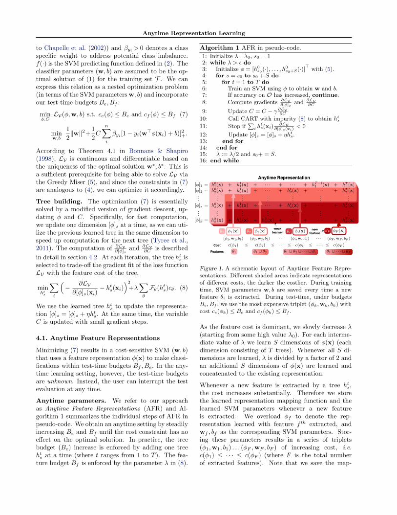
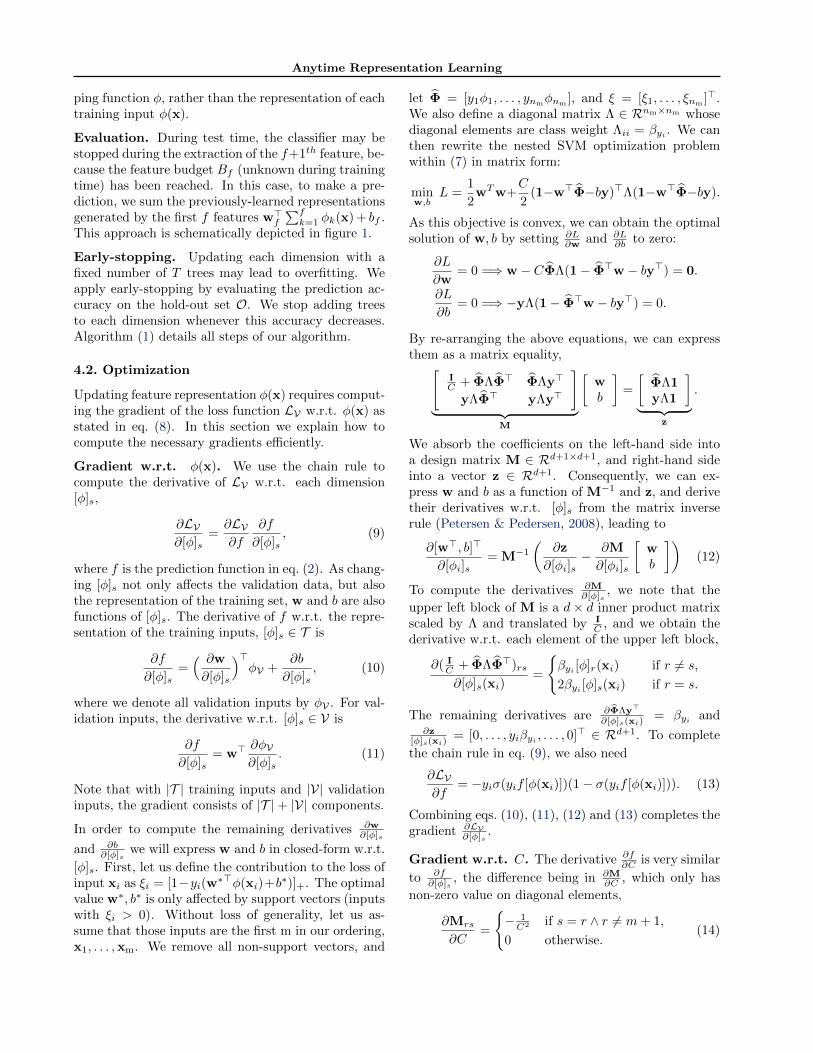
Figure 1. A schematic layout of Anytime Feature Repre-sentations. Different shaded areas indicate representationsof different costs, the darker the costlier. During trainingtime, SVM parameters w, b are saved every time a newfeature θi is extracted. During test-time, under budgetsBe, Bf , we use the most expensive triplet (φk,wk, bk) withcost ce(φk) ≤ Be and cf (φk) ≤ Bf .

As the feature cost is dominant, we slowly decrease λ(starting from some high value λ0). For each interme-diate value of λ we learn S dimensions of φ(x) (eachdimension consisting of T trees). Whenever all S di-mensions are learned, λ is divided by a factor of 2 andan additional S dimensions of φ(x) are learned andconcatenated to the existing representation.

Whenever a new feature is extracted by a tree hts,the cost increases substantially. Therefore we storethe learned representation mapping function and thelearned SVM parameters whenever a new featureis extracted. We overload φf to denote the rep-resentation learned with feature f th extracted, andwf , bf as the corresponding SVM parameters. Stor-ing these parameters results in a series of triplets(φ1,w1, b1) . . . (φF ,wF , bF ) of increasing cost, i.e.c(φ1) ≤ · · · ≤ c(φF ) (where F is the total numberof extracted features). Note that we save the map-

Anytime Representation Learning

ping function φ, rather than the representation of eachtraining input φ(x).

Evaluation. During test time, the classifier may bestopped during the extraction of the f+1th feature, be-cause the feature budget Bf (unknown during trainingtime) has been reached. In this case, to make a pre-diction, we sum the previously-learned representationsgenerated by the first f features w>f

∑fk=1 φk(x) + bf .

This approach is schematically depicted in figure 1.

Early-stopping. Updating each dimension with afixed number of T trees may lead to overfitting. Weapply early-stopping by evaluating the prediction ac-curacy on the hold-out set O. We stop adding treesto each dimension whenever this accuracy decreases.Algorithm (1) details all steps of our algorithm.

4.2. Optimization

Updating feature representation φ(x) requires comput-ing the gradient of the loss function LV w.r.t. φ(x) asstated in eq. (8). In this section we explain how tocompute the necessary gradients efficiently.

Gradient w.r.t. φ(x). We use the chain rule tocompute the derivative of LV w.r.t. each dimension[φ]s,

∂LV∂[φ]s

=∂LV∂f

∂f

∂[φ]s, (9)

where f is the prediction function in eq. (2). As chang-ing [φ]s not only affects the validation data, but alsothe representation of the training set, w and b are alsofunctions of [φ]s. The derivative of f w.r.t. the repre-sentation of the training inputs, [φ]s ∈ T is

∂f

∂[φ]s=( ∂w

∂[φ]s

)>φV +

∂b

∂[φ]s, (10)

where we denote all validation inputs by φV . For val-idation inputs, the derivative w.r.t. [φ]s ∈ V is

∂f

∂[φ]s= w>

∂φV∂[φ]s

. (11)

Note that with |T | training inputs and |V| validationinputs, the gradient consists of |T |+ |V| components.

In order to compute the remaining derivatives ∂w∂[φ]s

and ∂b∂[φ]s

we will express w and b in closed-form w.r.t.

[φ]s. First, let us define the contribution to the loss ofinput xi as ξi = [1−yi(w∗>φ(xi)+b∗)]+. The optimalvalue w∗, b∗ is only affected by support vectors (inputswith ξi > 0). Without loss of generality, let us as-sume that those inputs are the first m in our ordering,x1, . . . ,xm. We remove all non-support vectors, and

let Φ = [y1φ1, . . . , ynmφnm

], and ξ = [ξ1, . . . , ξnm]>.

We also define a diagonal matrix Λ ∈ Rnm×nm whosediagonal elements are class weight Λii = βyi . We canthen rewrite the nested SVM optimization problemwithin (7) in matrix form:

minw,b

L =1

2wTw+

C

2(1−w>Φ−by)>Λ(1−w>Φ−by).

As this objective is convex, we can obtain the optimalsolution of w, b by setting ∂L

∂w and ∂L∂b to zero:

∂L

∂w= 0 =⇒ w − CΦΛ(1− Φ>w − by>) = 0.

∂L

∂b= 0 =⇒ −yΛ(1− Φ>w − by>) = 0.

By re-arranging the above equations, we can expressthem as a matrix equality,[

IC + ΦΛΦ> ΦΛy>

yΛΦ> yΛy>

]︸ ︷︷ ︸

M

[wb

]=

[ΦΛ1yΛ1

]︸ ︷︷ ︸

z

.

We absorb the coefficients on the left-hand side intoa design matrix M ∈ Rd+1×d+1, and right-hand sideinto a vector z ∈ Rd+1. Consequently, we can ex-press w and b as a function of M−1 and z, and derivetheir derivatives w.r.t. [φ]s from the matrix inverserule (Petersen & Pedersen, 2008), leading to

∂[w>, b]>

∂[φi]s= M−1

(∂z

∂[φi]s− ∂M

∂[φi]s

[wb

])(12)

To compute the derivatives ∂M∂[φ]s

, we note that the

upper left block of M is a d× d inner product matrixscaled by Λ and translated by I

C , and we obtain thederivative w.r.t. each element of the upper left block,

∂( IC + ΦΛΦ>)rs

∂[φ]s(xi)=

{βyi [φ]r(xi) if r 6= s,

2βyi [φ]s(xi) if r = s.

The remaining derivatives are ∂ΦΛy>

∂[φ]s(xi)= βyi and

∂z[φ]s(xi)

= [0, . . . , yiβyi , . . . , 0]> ∈ Rd+1. To complete

the chain rule in eq. (9), we also need

∂LV∂f

= −yiσ(yif [φ(xi)])(1− σ(yif [φ(xi)])). (13)

Combining eqs. (10), (11), (12) and (13) completes thegradient ∂LV

∂[φ]s.

Gradient w.r.t. C. The derivative ∂f∂C is very similar

to ∂f∂[φ]s

, the difference being in ∂M∂C , which only has

non-zero value on diagonal elements,

∂Mrs

∂C=

{− 1C2 if s = r ∧ r 6= m+ 1,

0 otherwise.(14)

Anytime Representation Learning

Although computing the derivative requires the inver-sion of matrix M, M is only a (d + 1) × (d + 1) ma-trix. Because our algorithm converges after generatinga few (d ≈ 100) dimensions, the inverse operation isnot computationally intensive.

5. Results

We evaluate our algorithm on a synthetic data set inorder to demonstrate the AFR learning approach, aswell as two benchmark data sets from very different do-mains: the Yahoo! Learning to Rank Challenge dataset (Chapelle & Chang, 2011) and the Scene 15 recog-nition data set from Lazebnik et al. (2006).

Synthetic data. To visualize the learned anytimefeature representation, we construct a synthetic dataset as follows. We generate n = 1000 points (640for training/validation and 360 for testing) uniformlysampled from four different regions of two-dimensionalspace (as shown in figure 2, left). Each point is la-beled to be in class 1 or class 2 according to theXOR rule. These points are then randomly-projectedinto a ten-dimensional feature space (not shown).Each of these ten features is assigned an extractioncost: {1, 1, 1, 2, 5, 15, 25, 70, 100, 1000}. Correspond-ingly, each feature θ has zero-mean Gaussian noiseadded to it, with variance 1

cθ(where cθ is the cost of

feature θ). As such, cheap features are poorly repre-sentative of the classes while more expensive featuresmore accurately distinguish the two classes. To high-light the feature-selection capabilities of our techniquewe set the evaluation cost ce to 0. Using this data,we constrain the algorithm to learn a two-dimensionalanytime representation (i.e. φ(x) ∈ R2).

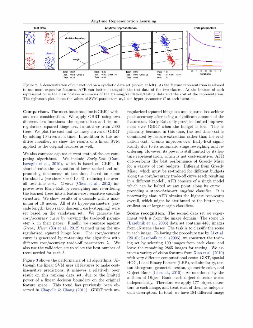
The center portion of figure 2 shows the anytime repre-sentations of testing points for various test-time bud-gets, as well as the learned hyperplane (black line),margins (gray lines) and classification accuracies. Asthe allowed feature cost budget is increased, AFRsteadily adjusts the representation and classifier tobetter distinguish the two classes. Using a small set offeatures (cost = 95) AFR can achieve nearly perfecttest accuracy and using all features AFR fully sepa-rates the test data.

The rightmost part of figure 2 shows how the learnedSVM classifier changes as the representation changes.The coefficients of the hyperplane w = [w1, w2]> ini-tially change drastically to appropriately weight theAFR features, then decrease gradually as more weaklearners are added to φ. Throughout, the hyper-parameter C is also optimized.

Yahoo Learning to Rank. The Yahoo! Learn-

0 2000 4000 6000 8000 10000 12000 14000 16000 180000.11

0.12

0.13

0.14

0.15

0.16

0.17

Linear SVMGBRT squared hinge loss (Friedman, 2001)GBRT squared loss (Friedman, 2001)Early−exit s=0.1 (Cambazoglu et. al. 2010)Early−exit s=0.3 (Cambazoglu et. al. 2010)Cronus (Chen et. al. 2012)Greedy Miser (Xu et. al. 2012)AFR

Cost

Pre

cisi

on @

5

Yahoo Learning to Rank

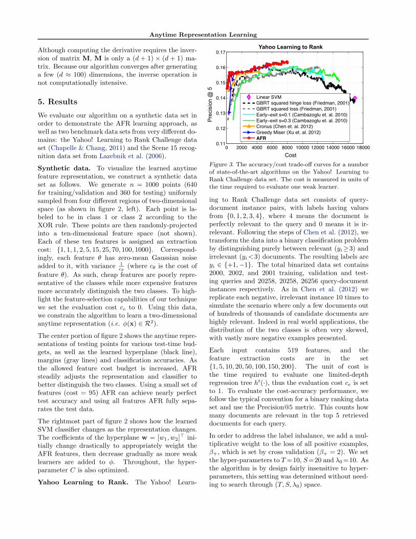
Figure 3. The accuracy/cost trade-off curves for a numberof state-of-the-art algorithms on the Yahoo! Learning toRank Challenge data set. The cost is measured in units ofthe time required to evaluate one weak learner.

ing to Rank Challenge data set consists of query-document instance pairs, with labels having valuesfrom {0, 1, 2, 3, 4}, where 4 means the document isperfectly relevant to the query and 0 means it is ir-relevant. Following the steps of Chen et al. (2012), wetransform the data into a binary classification problemby distinguishing purely between relevant (yi≥3) andirrelevant (yi<3) documents. The resulting labels areyi ∈ {+1,−1}. The total binarized data set contains2000, 2002, and 2001 training, validation and test-ing queries and 20258, 20258, 26256 query-documentinstances respectively. As in Chen et al. (2012) wereplicate each negative, irrelevant instance 10 times tosimulate the scenario where only a few documents outof hundreds of thousands of candidate documents arehighly relevant. Indeed in real world applications, thedistribution of the two classes is often very skewed,with vastly more negative examples presented.

Each input contains 519 features, and thefeature extraction costs are in the set{1, 5, 10, 20, 50, 100, 150, 200}. The unit of cost isthe time required to evaluate one limited-depthregression tree ht(·), thus the evaluation cost ce is setto 1. To evaluate the cost-accuracy performance, wefollow the typical convention for a binary ranking dataset and use the Precision@5 metric. This counts howmany documents are relevant in the top 5 retrieveddocuments for each query.

In order to address the label inbalance, we add a mul-tiplicative weight to the loss of all positive examples,β+, which is set by cross validation (β+ = 2). We setthe hyper-parameters to T =10, S=20 and λ0 =10. Asthe algorithm is by design fairly insensitive to hyper-parameters, this setting was determined without need-ing to search through (T, S, λ0) space.

Anytime Representation Learning

20 40 60 80 100 120 140

0

2

4

6

8

10

12

w1w2

bC

Anytime RepresentationTest Data

Cost 5

class 2class 1

0.820.820.76

TrainVal.Test

Cost 250.890.900.84

TrainVal.Test

Cost 950.990.990.98

TrainVal.Test

Cost 12201.01.01.0

TrainVal.Test

decision boundary

Iterations

SVM parameters

margin

Figure 2. A demonstration of our method on a synthetic data set (shown at left). As the feature representation is allowedto use more expensive features, AFR can better distinguish the test data of the two classes. At the bottom of eachrepresentation is the classification accuracies of the training/validation/testing data and the cost of the representation.The rightmost plot shows the values of SVM parameters w, b and hyper-parameter C at each iteration.

Comparison. The most basic baseline is GBRT with-out cost consideration. We apply GBRT using twodifferent loss functions: the squared loss and the un-regularized squared hinge loss. In total we train 2000trees. We plot the cost and accuracy curves of GBRTby adding 10 trees at a time. In addition to this ad-ditive classifier, we show the results of a linear SVMapplied to the original features as well.

We also compare against current state-of-the-art com-peting algorithms. We include Early-Exit (Cam-bazoglu et al., 2010), which is based on GBRT. Itshort-circuits the evaluation of lower ranked and un-promising documents at test-time, based on somethreshold s (we show s = 0.1, 0.3), reducing the over-all test-time cost. Cronus (Chen et al., 2012) im-proves over Early-Exit by reweighing and re-orderingthe learned trees into a feature-cost sensitive cascadestructure. We show results of a cascade with a max-imum of 10 nodes. All of its hyper-parameters (cas-cade length, keep ratio, discount, early-stopping) wereset based on the validation set. We generate thecost/accuracy curve by varying the trade-off param-eter λ, in their paper. Finally, we compare againstGreedy Miser (Xu et al., 2012) trained using the un-regularized squared hinge loss. The cost/accuracycurve is generated by re-training the algorithm withdifferent cost/accuracy trade-off parameters λ. Wealso use the validation set to select the best number oftrees needed for each λ.

Figure 3 shows the performance of all algorithms. Al-though the linear SVM uses all features to make cost-insensitive predictions, it achieves a relatively poorresult on this ranking data set, due to the limitedpower of a linear decision boundary on the originalfeature space. This trend has previously been ob-served in Chapelle & Chang (2011). GBRT with un-

regularized squared hinge loss and squared loss achievepeak accuracy after using a significant amount of thefeature set. Early-Exit only provides limited improve-ment over GBRT when the budget is low. This isprimarily because, in this case, the test-time cost isdominated by feature extraction rather than the eval-uation cost. Cronus improves over Early-Exit signif-icantly due to its automatic stage reweighing and re-ordering. However, its power is still limited by its fea-ture representation, which is not cost-sensitive. AFRout-performs the best performance of Greedy Miserfor a variety of cost budgets. Different from GreedyMiser, which must be re-trained for different budgetsalong the cost/accuracy trade-off curve (each resultingin a different model), AFR consists of a single modelwhich can be halted at any point along its curve—providing a state-of-the-art anytime classifier. It isnoteworthy that AFR obtains the highest test-scoresoverall, which might be attributed to the better gen-eralization of large-margin classifiers.

Scene recognition. The second data set we exper-iment with is from the image domain. The scene 15(Lazebnik et al., 2006) data set contains 4485 imagesfrom 15 scene classes. The task is to classify the scenein each image. Following the procedure use by Li et al.(2010); Lazebnik et al. (2006), we construct the train-ing set by selecting 100 images from each class, andleave the remaining 2865 images for testing. We ex-tract a variety of vision features from Xiao et al. (2010)with very different computational costs: GIST, spatialHOG, Local Binary Pattern (LBP), self-similarity, tex-ton histogram, geometric texton, geometric color, andObject Bank (Li et al., 2010). As mentioned by theauthors of Object Bank, each object detector worksindependently. Therefore we apply 177 object detec-tors to each image, and treat each of them as indepen-dent descriptors. In total, we have 184 different image

Anytime Representation Learning

0 5 10 15 20 25 30 350.45

0.5

0.55

0.6

0.65

0.7

0.75

0.8

GBRT squared hinge loss (Friedman, 2001)GBRT logistic loss (Friedman, 2001)SVM linear kernelEarly−ExitGreedy Miser (Xu et. al. 2012)AFR

Cost

Accuracy

Scene 15

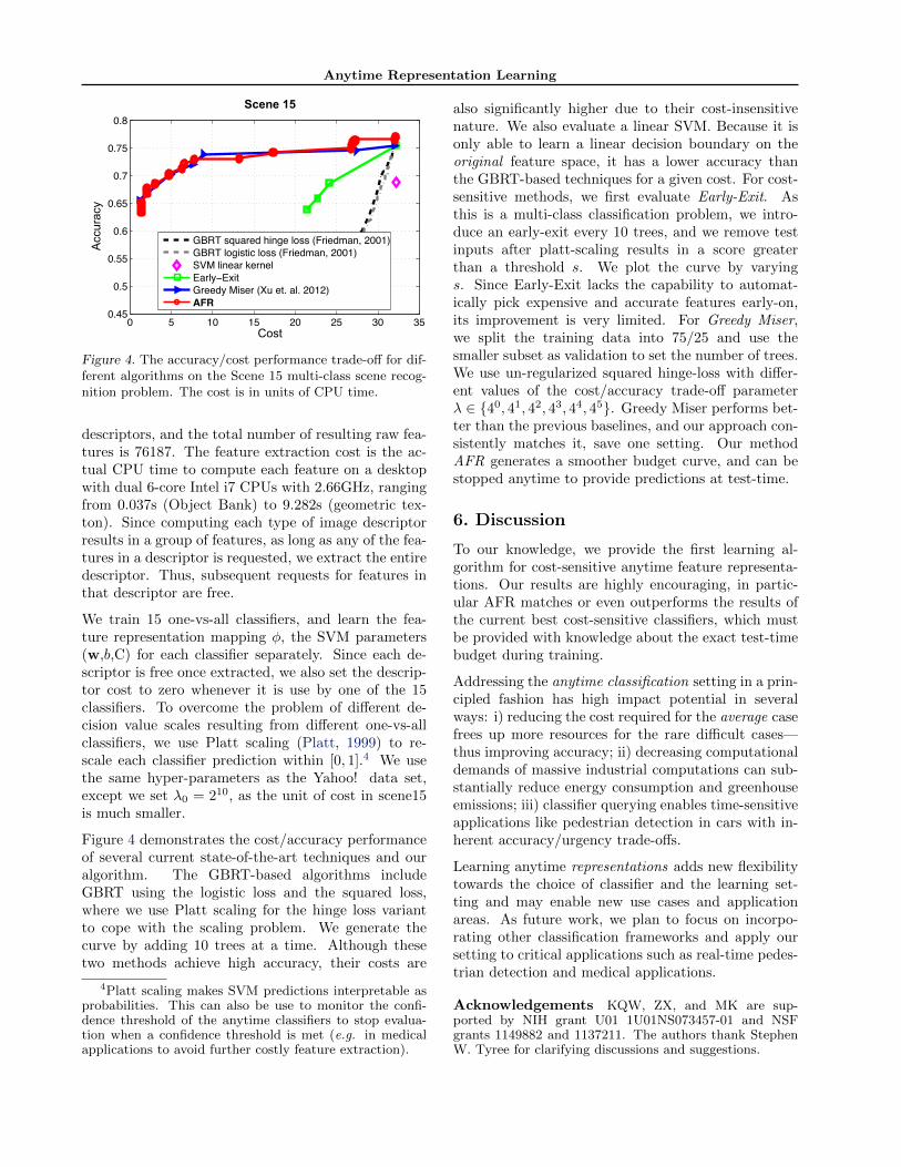
Figure 4. The accuracy/cost performance trade-off for dif-ferent algorithms on the Scene 15 multi-class scene recog-nition problem. The cost is in units of CPU time.

descriptors, and the total number of resulting raw fea-tures is 76187. The feature extraction cost is the ac-tual CPU time to compute each feature on a desktopwith dual 6-core Intel i7 CPUs with 2.66GHz, rangingfrom 0.037s (Object Bank) to 9.282s (geometric tex-ton). Since computing each type of image descriptorresults in a group of features, as long as any of the fea-tures in a descriptor is requested, we extract the entiredescriptor. Thus, subsequent requests for features inthat descriptor are free.

We train 15 one-vs-all classifiers, and learn the fea-ture representation mapping φ, the SVM parameters(w,b,C) for each classifier separately. Since each de-scriptor is free once extracted, we also set the descrip-tor cost to zero whenever it is use by one of the 15classifiers. To overcome the problem of different de-cision value scales resulting from different one-vs-allclassifiers, we use Platt scaling (Platt, 1999) to re-scale each classifier prediction within [0, 1].4 We usethe same hyper-parameters as the Yahoo! data set,except we set λ0 = 210, as the unit of cost in scene15is much smaller.

Figure 4 demonstrates the cost/accuracy performanceof several current state-of-the-art techniques and ouralgorithm. The GBRT-based algorithms includeGBRT using the logistic loss and the squared loss,where we use Platt scaling for the hinge loss variantto cope with the scaling problem. We generate thecurve by adding 10 trees at a time. Although thesetwo methods achieve high accuracy, their costs are

4Platt scaling makes SVM predictions interpretable asprobabilities. This can also be use to monitor the confi-dence threshold of the anytime classifiers to stop evalua-tion when a confidence threshold is met (e.g. in medicalapplications to avoid further costly feature extraction).

also significantly higher due to their cost-insensitivenature. We also evaluate a linear SVM. Because it isonly able to learn a linear decision boundary on theoriginal feature space, it has a lower accuracy thanthe GBRT-based techniques for a given cost. For cost-sensitive methods, we first evaluate Early-Exit. Asthis is a multi-class classification problem, we intro-duce an early-exit every 10 trees, and we remove testinputs after platt-scaling results in a score greaterthan a threshold s. We plot the curve by varyings. Since Early-Exit lacks the capability to automat-ically pick expensive and accurate features early-on,its improvement is very limited. For Greedy Miser,we split the training data into 75/25 and use thesmaller subset as validation to set the number of trees.We use un-regularized squared hinge-loss with differ-ent values of the cost/accuracy trade-off parameterλ ∈ {40, 41, 42, 43, 44, 45}. Greedy Miser performs bet-ter than the previous baselines, and our approach con-sistently matches it, save one setting. Our methodAFR generates a smoother budget curve, and can bestopped anytime to provide predictions at test-time.

6. Discussion

To our knowledge, we provide the first learning al-gorithm for cost-sensitive anytime feature representa-tions. Our results are highly encouraging, in partic-ular AFR matches or even outperforms the results ofthe current best cost-sensitive classifiers, which mustbe provided with knowledge about the exact test-timebudget during training.

Addressing the anytime classification setting in a prin-cipled fashion has high impact potential in severalways: i) reducing the cost required for the average casefrees up more resources for the rare difficult cases—thus improving accuracy; ii) decreasing computationaldemands of massive industrial computations can sub-stantially reduce energy consumption and greenhouseemissions; iii) classifier querying enables time-sensitiveapplications like pedestrian detection in cars with in-herent accuracy/urgency trade-offs.

Learning anytime representations adds new flexibilitytowards the choice of classifier and the learning set-ting and may enable new use cases and applicationareas. As future work, we plan to focus on incorpo-rating other classification frameworks and apply oursetting to critical applications such as real-time pedes-trian detection and medical applications.

Acknowledgements KQW, ZX, and MK are sup-ported by NIH grant U01 1U01NS073457-01 and NSFgrants 1149882 and 1137211. The authors thank StephenW. Tyree for clarifying discussions and suggestions.

Anytime Representation Learning

References

Bonnans, J Frederic and Shapiro, Alexander. Optimizationproblems with perturbations: A guided tour. SIAM re-view, 40(2):228–264, 1998.

Breiman, L. Classification and regression trees. Chapman& Hall/CRC, 1984.

Busa-Fekete, R., Benbouzid, D., Kegl, B., et al. Fast clas-sification using sparse decision dags. In ICML, 2012.

Cambazoglu, B.B., Zaragoza, H., Chapelle, O., Chen, J.,Liao, C., Zheng, Z., and Degenhardt, J. Early exit opti-mizations for additive machine learned ranking systems.In WSDM’3, pp. 411–420, 2010.

Chapelle, O. and Chang, Y. Yahoo! learning to rank chal-lenge overview. In JMLR: Workshop and ConferenceProceedings, volume 14, pp. 1–24, 2011.

Chapelle, O., Vapnik, V., Bousquet, O., and Mukherjee,S. Choosing multiple parameters for support vector ma-chines. Machine Learning, 46(1):131–159, 2002.

Chapelle, O., Shivaswamy, P., Vadrevu, S., Weinberger, K.,Zhang, Y., and Tseng, B. Boosted multi-task learning.Machine learning, 85(1):149–173, 2011.

Chen, M., Xu, Z., Weinberger, K. Q., and Chapelle, O.Classifier cascade for minimizing feature evaluation cost.In AISTATS, 2012.

Cortes, C. and Vapnik, V. Support-vector networks. Ma-chine learning, 20(3):273–297, 1995.

Dekel, Ofer, Shalev-Shwartz, Shai, and Singer, Yoram. Theforgetron: A kernel-based perceptron on a budget. SIAMJournal on Computing, 37(5):1342–1372, 2008.

Dredze, M., Gevaryahu, R., and Elias-Bachrach, A. Learn-ing fast classifiers for image spam. In proceedings of theConference on Email and Anti-Spam (CEAS), 2007.

Freund, Y. and Schapire, R. A desicion-theoretic gen-eralization of on-line learning and an application toboosting. In Computational learning theory, pp. 23–37.Springer, 1995.

Friedman, J.H. Greedy function approximation: a gradientboosting machine. The Annals of Statistics, pp. 1189–1232, 2001.

Gao, T. and Koller, D. Active classification based on valueof classifier. In NIPS, pp. 1062–1070. 2011a.

Gao, Tianshi and Koller, Daphne. Multiclass boosting withhinge loss based on output coding. ICML ’11, pp. 569–576, 2011b.

Gavrila, D. Pedestrian detection from a moving vehicle.ECCV 2000, pp. 37–49, 2000.

Grubb, A. and Bagnell, J. A. Speedboost: Anytime predic-tion with uniform near-optimality. In AISTATS, 2012.

Grubb, A. and Bagnell, J.A. Generalized boostingalgorithms for convex optimization. arXiv preprintarXiv:1105.2054, 2011.

Grubb, Alexander and Bagnell, J Andrew. Boosted back-propagation learning for training deep modular net-works. In Proceedings of the International Conferenceon Machine Learning (27th ICML), 2010.

Kedem, Dor, Tyree, Stephen, Weinberger, Kilian Q., Sha,

Fei, and Lanckriet, Gert. Non-linear metric learning. InNIPS, pp. 2582–2590. 2012.

Lazebnik, S., Schmid, C., and Ponce, J. Beyond bags offeatures: Spatial pyramid matching for recognizing nat-ural scene categories. In CVPR, pp. 2169–2178, 2006.

Lefakis, L. and Fleuret, F. Joint cascade optimization usinga product of boosted classifiers. In NIPS, pp. 1315–1323.2010.

Li, L.J., Su, H., Xing, E.P., and Fei-Fei, L. Object bank:A high-level image representation for scene classificationand semantic feature sparsification. NIPS, 2010.

Mohan, A., Chen, Z., and Weinberger, K. Q. Web-search ranking with initialized gradient boosted regres-sion trees. JMLR: Workshop and Conference Proceed-ings, 14:77–89, 2011.

Petersen, K. B. and Pedersen, M. S. The matrix cookbook,Oct 2008.

Platt, J.C. Fast training of support vector machines usingsequential minimal optimization. 1999.

Pujara, J., Daume III, H., and Getoor, L. Using classi-fier cascades for scalable e-mail classification. In CEAS,2011.

Raykar, V.C., Krishnapuram, B., and Yu, S. Designingefficient cascaded classifiers: tradeoff between accuracyand cost. In ACM SIGKDD, pp. 853–860, 2010.

Saberian, M. and Vasconcelos, N. Boosting classifier cas-cades. In NIPS, pp. 2047–2055. 2010.

Trzcinski, Tomasz, Christoudias, Mario, Lepetit, Vincent,and Fua, Pascal. Learning image descriptors with theboosting-trick. In NIPS, pp. 278–286. 2012.

Tyree, S., Weinberger, K.Q., Agrawal, K., and Paykin, J.Parallel boosted regression trees for web search ranking.In WWW, pp. 387–396. ACM, 2011.

Viola, P. and Jones, M.J. Robust real-time face detection.IJCV, 57(2):137–154, 2004.

Wang, J. and Saligrama, V. Local supervised learningthrough space partitioning. In NIPS, pp. 91–99, 2012.

Weinberger, K.Q., Dasgupta, A., Langford, J., Smola, A.,and Attenberg, J. Feature hashing for large scale multi-task learning. In ICML, pp. 1113–1120, 2009.

Xiao, Jianxiong, Hays, James, Ehinger, Krista A, Oliva,Aude, and Torralba, Antonio. Sun database: Large-scale scene recognition from abbey to zoo. In CVPR,pp. 3485–3492. IEEE, 2010.

Xu, Z., Weinberger, K.Q., and Chapelle, O. The greedymiser: Learning under test-time budgets. In ICML, pp.1175–1182, 2012.

Xu, Zhixiang, Kusner, Matt J., Weinberger, Kilian Q., andChen, Minmin. Cost-sensitive tree of classifiers. In Das-gupta, Sanjoy and McAllester, David (eds.), ICML ’13,pp. to appear, 2013.

Zheng, Z., Zha, H., Zhang, T., Chapelle, O., Chen, K., andSun, G. A general boosting method and its applicationto learning ranking functions for web search. In NIPS,pp. 1697–1704. Cambridge, MA, 2008.