antennas tutorial basics

7/14/2019 Antennas Tutorial Basics.

http://slidepdf.com/reader/full/antennas-tutorial-basics 1/16

Antennas

Some Properties and Principles of Antennas

An antenna may be viewed as a transducer used to match the transmission line to the

surrounding medium or vice versa. (Sadiku 588)

Transmission lines are designed to guide electromagnetic energy with a minimum of radiation. All antennas involve the same basic principle that radiation is produced byaccelerated (or decelerated) charge. (Kraus 5th ed 247) Note: Time-varying current meansthat electrons are accelerated and decelerated.

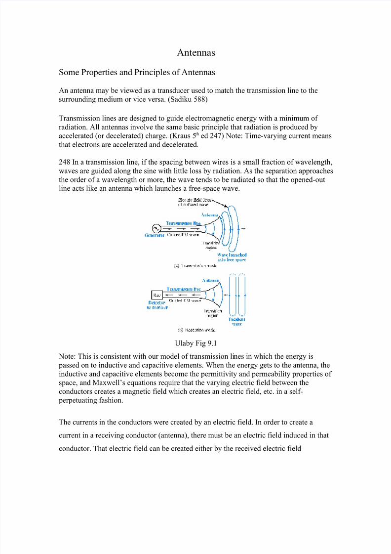
248 In a transmission line, if the spacing between wires is a small fraction of wavelength,waves are guided along the sine with little loss by radiation. As the separation approachesthe order of a wavelength or more, the wave tends to be radiated so that the opened-outline acts like an antenna which launches a free-space wave.

Ulaby Fig 9.1

Note: This is consistent with our model of transmission lines in which the energy is passed on to inductive and capacitive elements. When the energy gets to the antenna, theinductive and capacitive elements become the permittivity and permeability properties of space, and Maxwell’s equations require that the varying electric field between theconductors creates a magnetic field which creates an electric field, etc. in a self- perpetuating fashion.

The currents in the conductors were created by an electric field. In order to create a

current in a receiving conductor (antenna), there must be an electric field induced in that

conductor. That electric field can be created either by the received electric field



component or by the magnetic field component or a combination of both. We will focus

on the electric field component.

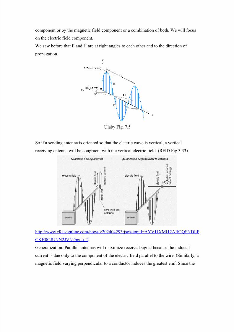
We saw before that E and H are at right angles to each other and to the direction of

propagation.

Ulaby Fig. 7.5

So if a sending antenna is oriented so that the electric wave is vertical, a vertical

receiving antenna will be congruent with the vertical electric field. (RFID Fig 3.33)

http://www.rfdesignline.com/howto/202404293;jsessionid=AYVJ1XMI12AROQSNDLPCKH0CJUNN2JVN?pgno=2

Generalization: Parallel antennas will maximize received signal because the induced

current is due only to the component of the electric field parallel to the wire. (Similarly, a

magnetic field varying perpendicular to a conductor induces the greatest emf. Since the







orientation of the magnetic field is perpendicular to the electric field, one can think of the

electric field as having been generated by the magnetic field.)

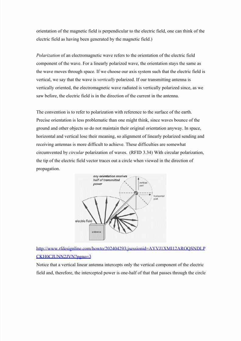
Polarization of an electromagnetic wave refers to the orientation of the electric field

component of the wave. For a linearly polarized wave, the orientation stays the same as

the wave moves through space. If we choose our axis system such that the electric field is

vertical, we say that the wave is vertically polarized. If our transmitting antenna is

vertically oriented, the electromagnetic wave radiated is vertically polarized since, as we

saw before, the electric field is in the direction of the current in the antenna.

The convention is to refer to polarization with reference to the surface of the earth.

Precise orientation is less problematic than one might think, since waves bounce of theground and other objects so do not maintain their original orientation anyway. In space,

horizontal and vertical lose their meaning, so alignment of linearly polarized sending and

receiving antennas is more difficult to achieve. These difficulties are somewhat

circumvented by circular polarization of waves. (RFID 3.34) With circular polarization,

the tip of the electric field vector traces out a circle when viewed in the direction of

propagation.

http://www.rfdesignline.com/howto/202404293;jsessionid=AYVJ1XMI12AROQSNDLP

CKH0CJUNN2JVN?pgno=3

Notice that a vertical linear antenna intercepts only the vertical component of the electric

field and, therefore, the intercepted power is one-half of that that passes through the circle







that bounds the circle containing the antenna. With this configuration, however,

orientation of the receiving antenna is less critical; there will be no “dead signal”

orientations.

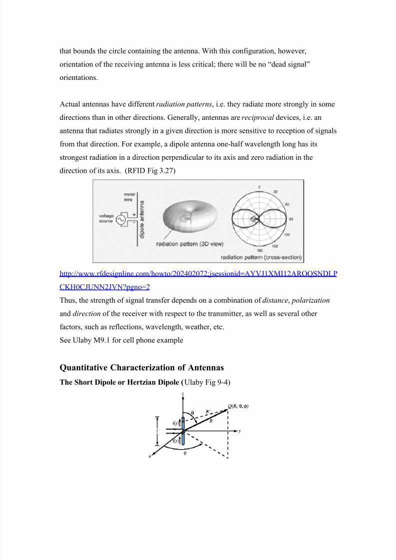
Actual antennas have different radiation patterns, i.e. they radiate more strongly in some

directions than in other directions. Generally, antennas are reciprocal devices, i.e. an

antenna that radiates strongly in a given direction is more sensitive to reception of signals

from that direction. For example, a dipole antenna one-half wavelength long has its

strongest radiation in a direction perpendicular to its axis and zero radiation in the

direction of its axis. (RFID Fig 3.27)

http://www.rfdesignline.com/howto/202402072;jsessionid=AYVJ1XMI12AROQSNDLP

CKH0CJUNN2JVN?pgno=2

Thus, the strength of signal transfer depends on a combination of distance, polarization

and direction of the receiver with respect to the transmitter, as well as several other

factors, such as reflections, wavelength, weather, etc.

See Ulaby M9.1 for cell phone example

Quantitative Characterization of Antennas

The Short Dipole or Hertzian Dipole (Ulaby Fig 9-4)







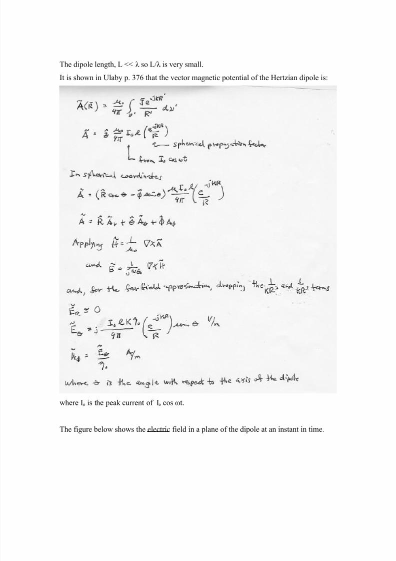
The dipole length, L << λ so L/λ is very small.

It is shown in Ulaby p. 376 that the vector magnetic potential of the Hertzian dipole is:

where Io is the peak current of Io cos ωt.

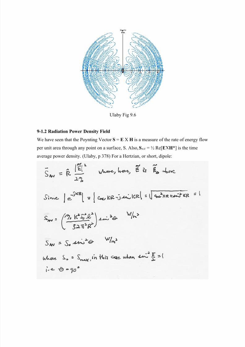
The figure below shows the electric field in a plane of the dipole at an instant in time.



Ulaby Fig 9.6

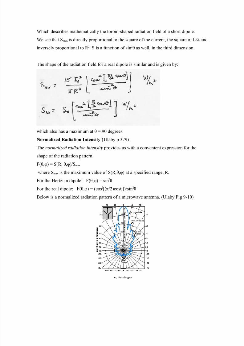
9-1.2 Radiation Power Density Field

We have seen that the Poynting Vector S = E X H is a measure of the rate of energy flow

per unit area through any point on a surface, S. Also, SAV = ½ Re[EXH*] is the time

average power density. (Ulaby, p 378) For a Hertzian, or short, dipole:



Which describes mathematically the toroid-shaped radiation field of a short dipole.

We see that Smax is directly proportional to the square of the current, the square of L/λ and

inversely proportional to R 2. S is a function of sin2θ as well, in the third dimension.

The shape of the radiation field for a real dipole is similar and is given by:

which also has a maximum at θ = 90 degrees.

Normalized Radiation Intensity (Ulaby p 379)

The normalized radiation intensity provides us with a convenient expression for the

shape of the radiation pattern.

F(θ,φ) = S(R, θ,φ)/Smax

where Smax is the maximum value of S(R,θ,φ) at a specified range, R.

For the Hertzian dipole: F(θ,φ) = sin2

θFor the real dipole: F(θ,φ) = (cos2[(π/2)cosθ])/sin2θ

Below is a normalized radiation pattern of a microwave antenna. (Ulaby Fig 9-10)



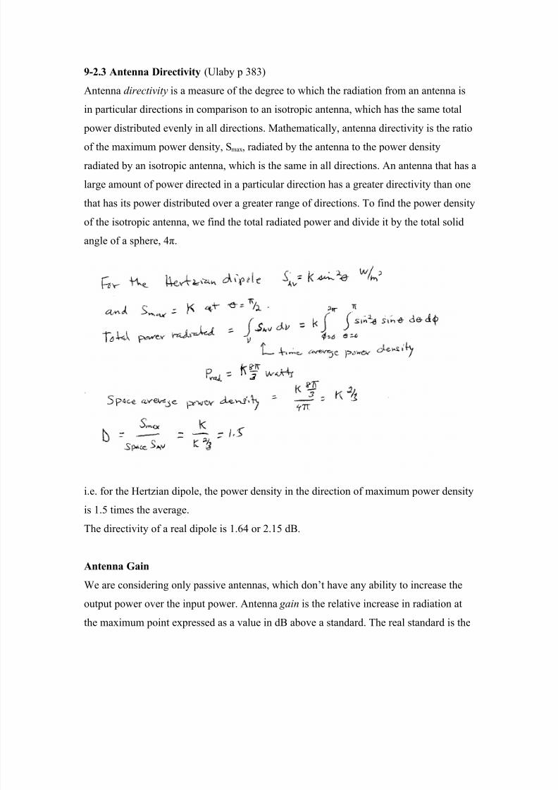
9-2.3 Antenna Directivity (Ulaby p 383)

Antenna directivity is a measure of the degree to which the radiation from an antenna is

in particular directions in comparison to an isotropic antenna, which has the same total

power distributed evenly in all directions. Mathematically, antenna directivity is the ratio

of the maximum power density, Smax, radiated by the antenna to the power density

radiated by an isotropic antenna, which is the same in all directions. An antenna that has a

large amount of power directed in a particular direction has a greater directivity than one

that has its power distributed over a greater range of directions. To find the power density

of the isotropic antenna, we find the total radiated power and divide it by the total solid

angle of a sphere, 4π.

i.e. for the Hertzian dipole, the power density in the direction of maximum power density

is 1.5 times the average.

The directivity of a real dipole is 1.64 or 2.15 dB.

Antenna Gain

We are considering only passive antennas, which don’t have any ability to increase the

output power over the input power. Antenna gain is the relative increase in radiation at

the maximum point expressed as a value in dB above a standard. The real standard is the



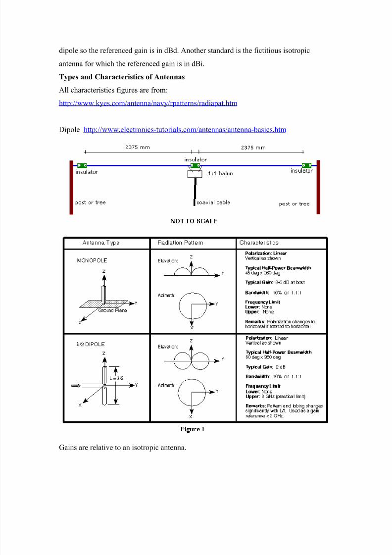
dipole so the referenced gain is in dBd. Another standard is the fictitious isotropic

antenna for which the referenced gain is in dBi.

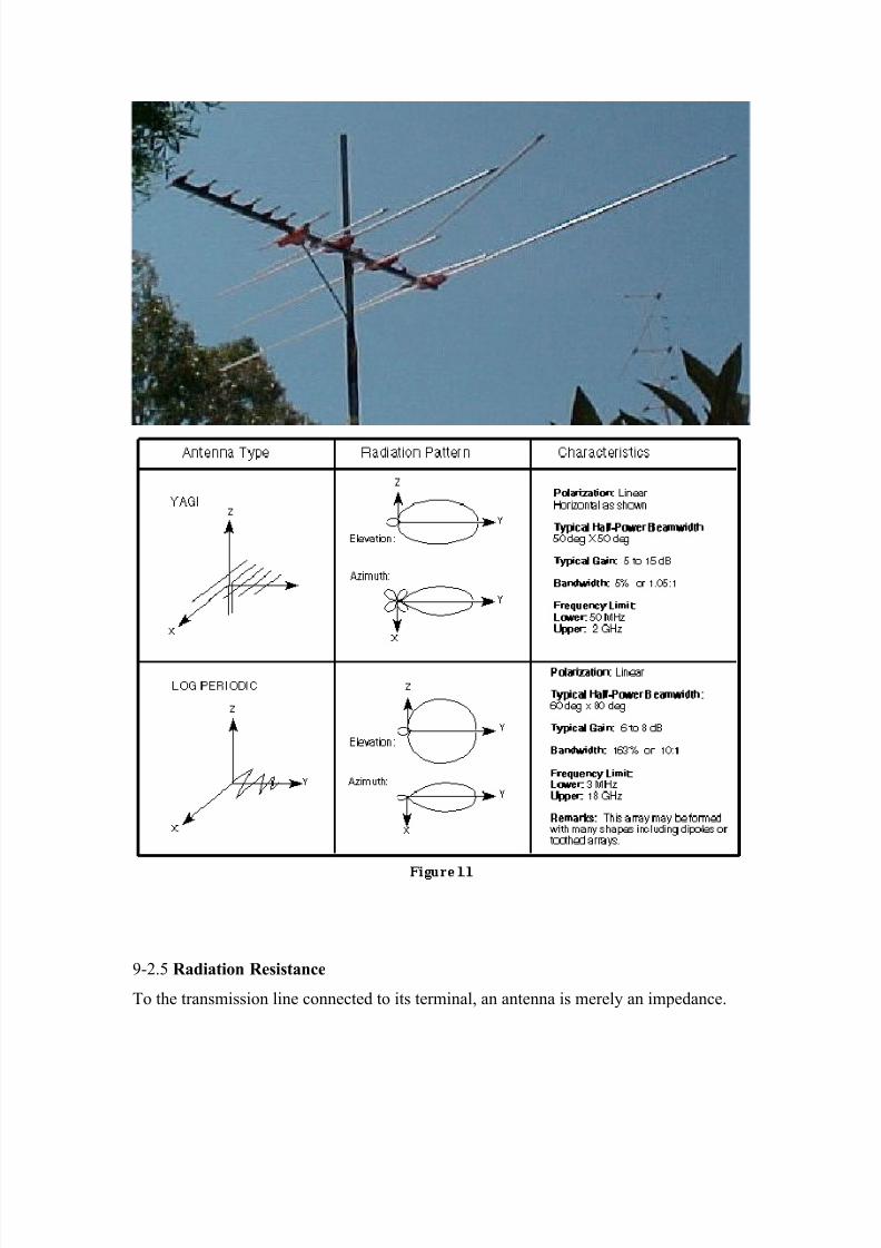
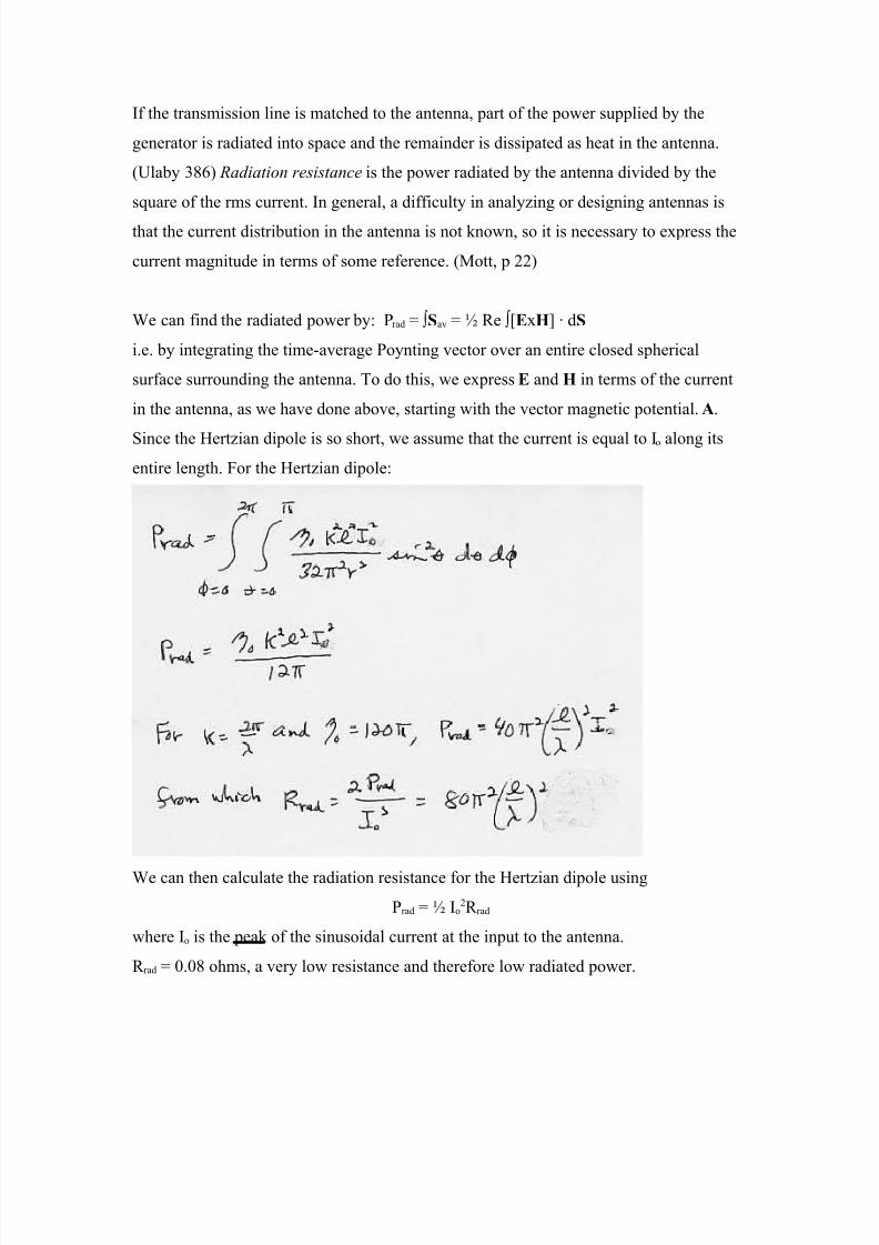
Types and Characteristics of Antennas

All characteristics figures are from:

http://www.kyes.com/antenna/navy/rpatterns/radiapat.htm

Dipole http://www.electronics-tutorials.com/antennas/antenna-basics.htm

Gains are relative to an isotropic antenna.


http://www.electronics-tutorials.com/antennas/antenna-basics.htm






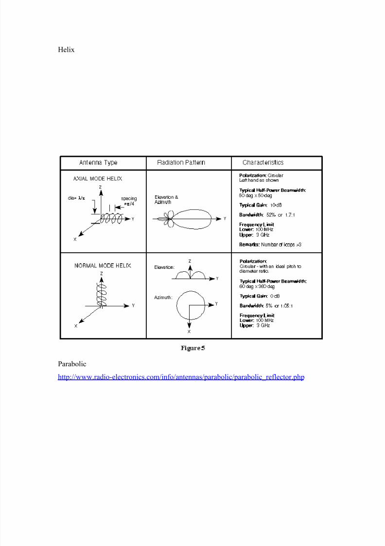
Helix

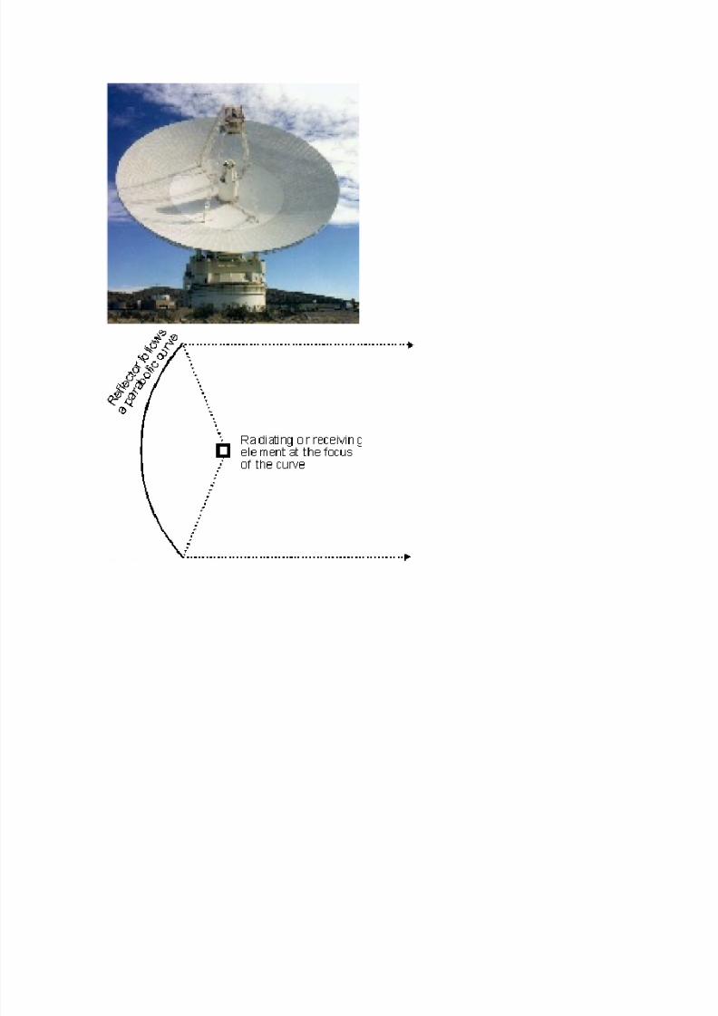
Parabolic

http://www.radio-electronics.com/info/antennas/parabolic/parabolic_reflector.php





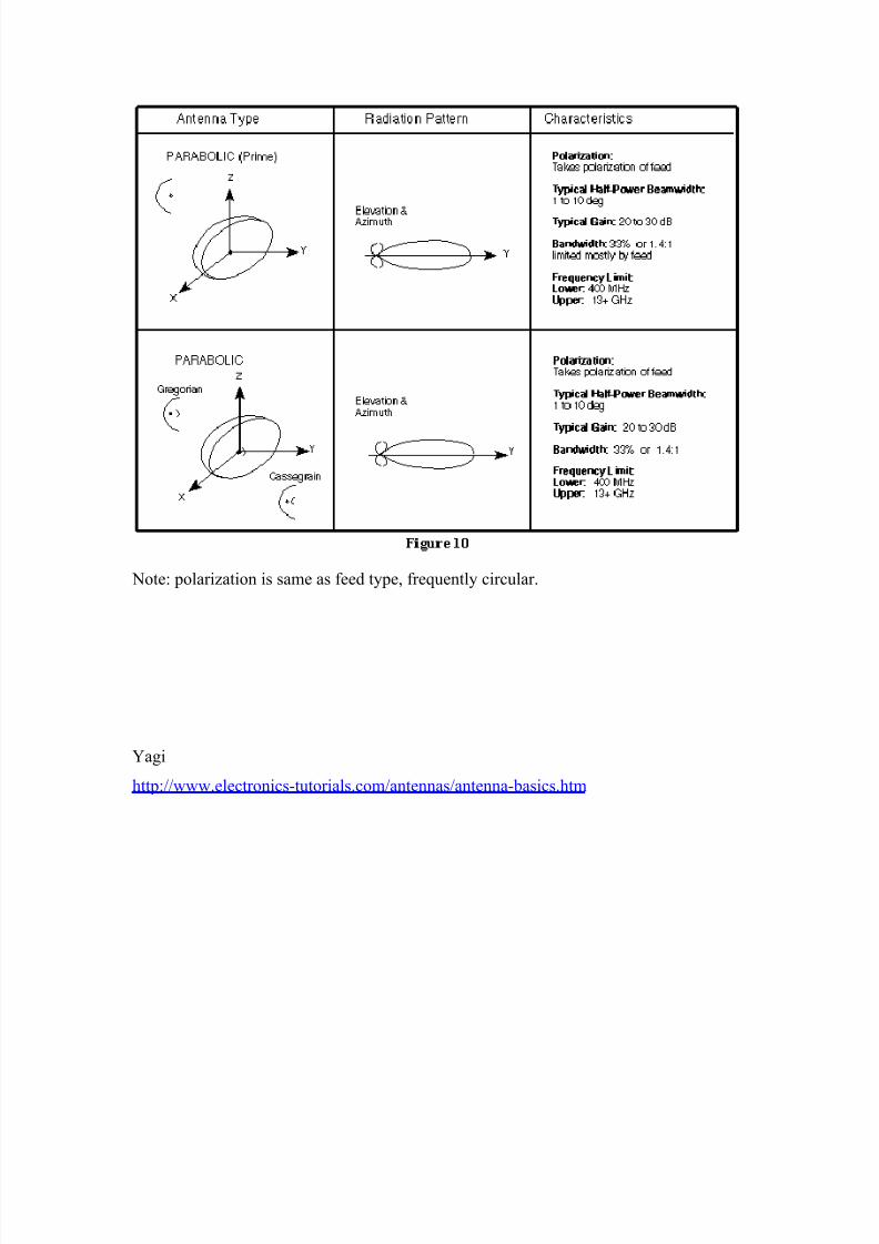
Note: polarization is same as feed type, frequently circular.

Yagi






9-2.5 Radiation Resistance

To the transmission line connected to its terminal, an antenna is merely an impedance.



If the transmission line is matched to the antenna, part of the power supplied by the

generator is radiated into space and the remainder is dissipated as heat in the antenna.

(Ulaby 386) Radiation resistance is the power radiated by the antenna divided by the

square of the rms current. In general, a difficulty in analyzing or designing antennas is

that the current distribution in the antenna is not known, so it is necessary to express the

current magnitude in terms of some reference. (Mott, p 22)

We can find the radiated power by: Prad = ∫Sav = ½ Re ∫[ExH] ∙ dS

i.e. by integrating the time-average Poynting vector over an entire closed spherical

surface surrounding the antenna. To do this, we express E and H in terms of the current

in the antenna, as we have done above, starting with the vector magnetic potential. A.

Since the Hertzian dipole is so short, we assume that the current is equal to Io along itsentire length. For the Hertzian dipole:

We can then calculate the radiation resistance for the Hertzian dipole using

Prad = ½ Io2R rad

where Io is the peak of the sinusoidal current at the input to the antenna.

R rad = 0.08 ohms, a very low resistance and therefore low radiated power.



The calculation of radiated power and radiation resistance for a dipole antenna is

somewhat more complicated; but is simpler than for most other antennas. In the case of

linear wire antennas, it has been found that the current behaves approximately as it does

on a transmission line. (Schwarz 353) It has been found from experimental

measurements that the current distribution on a dipole antenna is approximately:

I = Io sin[(2π/λ)(L/2 +-y)]

Where Io is the current at its point of maximum, and where +y is used when y<0 and –y

when y>0. For the half-wave dipole, L=λ/2 and I=Io at the center (y=0) and I = 0 at the

ends. (Kraus p 285)

It is shown (Ulaby p 389) that for a half-wave dipole, R rad = 73 ohms, approximately

equal to the standard 75 ohm transmission line, designed to match a half-wave dipole.

Antenna Impedance and Matching

Radiation resistance and ohmic resistance is only part of the antenna impedance.

Inductive and capacitive reactance can be present. Energy that is transferred to the near

field relates to the reactive component of the current in the antenna. This is the 1/R 2

component of the electric and magnetic fields that we neglected when deriving the

expressions for the far fields.

There are a variety of complex models for antenna impedance.

See http://www.ewh.ieee.org/r6/scv/aps/index_files/Stearns_APS_031406.pdf

We will use simple approximate models – series and parallel RLC circuits.

See http://www.borg.com/~warrend/guru.html

When the dipole is very short (in terms of physical length relative to wavelength), the

dipole can be modeled as a series RLC circuit in which the impedance is dominated by

radiation resistance and capacitive reactance. As the antenna is made longer, R rad and XL

increase and XC decreases. When the physical length equals λ/2, XL = XC with a resulting

impedance of R rad. As the antenna is made longer than λ/2, the model is a parallel RLC

circuit. When length equals λ, the tank LC circuit has infinite impedance, leaving the

parallel R rad as the net impedance. Between a length of λ and 3λ/2, the model is a series

RLC circuit, and so forth.

http://www.ewh.ieee.org/r6/scv/aps/index_files/Stearns_APS_031406.pdf

http://www.borg.com/~warrend/guru.html


http://www.ewh.ieee.org/r6/scv/aps/index_files/Stearns_APS_031406.pdf




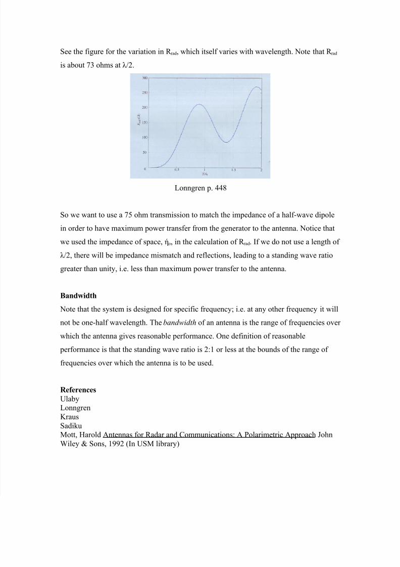
See the figure for the variation in R rad, which itself varies with wavelength. Note that R rad

is about 73 ohms at λ/2.

Lonngren p. 448

So we want to use a 75 ohm transmission to match the impedance of a half-wave dipole

in order to have maximum power transfer from the generator to the antenna. Notice that

we used the impedance of space, ήo, in the calculation of R rad. If we do not use a length of

λ/2, there will be impedance mismatch and reflections, leading to a standing wave ratio

greater than unity, i.e. less than maximum power transfer to the antenna.

Bandwidth Note that the system is designed for specific frequency; i.e. at any other frequency it will

not be one-half wavelength. The bandwidth of an antenna is the range of frequencies over

which the antenna gives reasonable performance. One definition of reasonable

performance is that the standing wave ratio is 2:1 or less at the bounds of the range of

frequencies over which the antenna is to be used.

References

UlabyLonngrenKrausSadikuMott, Harold Antennas for Radar and Communications: A Polarimetric Approach JohnWiley & Sons, 1992 (In USM library)

antennas tutorial basics

Documents