ansys mechanical tutorials - university of...
TRANSCRIPT

ANSYS Mechanical Tutorials
Release 16.0ANSYS, Inc.January 2015Southpointe
2600 ANSYS DriveCanonsburg, PA 15317 ANSYS, Inc. is
certified to ISO9001:2008.
[email protected]://www.ansys.com(T) 724-746-3304(F) 724-514-9494

Copyright and Trademark Information
© 2014-2015 SAS IP, Inc. All rights reserved. Unauthorized use, distribution or duplication is prohibited.
ANSYS, ANSYS Workbench, Ansoft, AUTODYN, EKM, Engineering Knowledge Manager, CFX, FLUENT, HFSS, AIMand any and all ANSYS, Inc. brand, product, service and feature names, logos and slogans are registered trademarksor trademarks of ANSYS, Inc. or its subsidiaries in the United States or other countries. ICEM CFD is a trademarkused by ANSYS, Inc. under license. CFX is a trademark of Sony Corporation in Japan. All other brand, product,service and feature names or trademarks are the property of their respective owners.
Disclaimer Notice
THIS ANSYS SOFTWARE PRODUCT AND PROGRAM DOCUMENTATION INCLUDE TRADE SECRETS AND ARE CONFID-ENTIAL AND PROPRIETARY PRODUCTS OF ANSYS, INC., ITS SUBSIDIARIES, OR LICENSORS. The software productsand documentation are furnished by ANSYS, Inc., its subsidiaries, or affiliates under a software license agreementthat contains provisions concerning non-disclosure, copying, length and nature of use, compliance with exportinglaws, warranties, disclaimers, limitations of liability, and remedies, and other provisions. The software productsand documentation may be used, disclosed, transferred, or copied only in accordance with the terms and conditionsof that software license agreement.
ANSYS, Inc. is certified to ISO 9001:2008.
U.S. Government Rights
For U.S. Government users, except as specifically granted by the ANSYS, Inc. software license agreement, the use,duplication, or disclosure by the United States Government is subject to restrictions stated in the ANSYS, Inc.software license agreement and FAR 12.212 (for non-DOD licenses).
Third-Party Software
See the legal information in the product help files for the complete Legal Notice for ANSYS proprietary softwareand third-party software. If you are unable to access the Legal Notice, please contact ANSYS, Inc.
Published in the U.S.A.
Table of Contents
Tutorials ... . . . . . . . . . . . . . . . . . . . . . . . . . . . . . . . . . . . . . . . . . . . . . . . . . . . . . . . . . . . . . . . . . . . . . . . . . . . . . . . . . . . . . . . . . . . . . . . . . . . . . . . . . . . . . . . . . . . . . . . . . . . . . . . . . . . . . . . . . . . . . . . . . . . . vActuator Mechanism using Rigid Body Dynamics . . . . . . . . . . . . . . . . . . . . . . . . . . . . . . . . . . . . . . . . . . . . . . . . . . . . . . . . . . . . . . . . . . . . . . . . . . . . . . . . . . . . . 1Nonlinear Static Structural Analysis of a Rubber Boot Seal . . . . . . . . . . . . . . . . . . . . . . . . . . . . . . . . . . . . . . . . . . . . . . . . . . . . . . . . . . . . . . . . . . . . . 11Cyclic Symmetry Analysis of a Rotor - Brake Assembly . . . . . . . . . . . . . . . . . . . . . . . . . . . . . . . . . . . . . . . . . . . . . . . . . . . . . . . . . . . . . . . . . . . . . . . . . . . . 35Steady-State and Transient Thermal Analysis of a Circuit Board . . . . . . . . . . . . . . . . . . . . . . . . . . . . . . . . . . . . . . . . . . . . . . . . . . . . . . . . . . . . . 51Delamination Analysis using Contact Based Debonding Capability . . . . . . . . . . . . . . . . . . . . . . . . . . . . . . . . . . . . . . . . . . . . . . . . . . . . . . . 61Interface Delamination Analysis of Double Cantilever Beam . . . . . . . . . . . . . . . . . . . . . . . . . . . . . . . . . . . . . . . . . . . . . . . . . . . . . . . . . . . . . . . . . . 77Fracture Analysis of a 2D Cracked Specimen using Pre-Meshed Crack . . . . . . . . . . . . . . . . . . . . . . . . . . . . . . . . . . . . . . . . . . . . . . . . . . . . 97Fracture Analysis of a Double Cantilever Beam (DCB) using Pre-Meshed Crack . . . . . . . . . . . . . . . . . . . . . . . . . . . . . . . . . . . . 107Fracture Analysis of an X-Joint Problem with Surface Flaw using Internally Generated Crack Mesh . . . . 113Using Finite Element Access to Resolve Overconstraint . . . . . . . . . . . . . . . . . . . . . . . . . . . . . . . . . . . . . . . . . . . . . . . . . . . . . . . . . . . . . . . . . . . . . . . . . 121Simple Pendulum using Rigid Dynamics and Nonlinear Bushing . . . . . . . . . . . . . . . . . . . . . . . . . . . . . . . . . . . . . . . . . . . . . . . . . . . . . . . . . . 153Track Roller Mechanism using Point on Curve Joints and Rigid Body Dynamics . . . . . . . . . . . . . . . . . . . . . . . . . . . . . . . . . . 159Index .... . . . . . . . . . . . . . . . . . . . . . . . . . . . . . . . . . . . . . . . . . . . . . . . . . . . . . . . . . . . . . . . . . . . . . . . . . . . . . . . . . . . . . . . . . . . . . . . . . . . . . . . . . . . . . . . . . . . . . . . . . . . . . . . . . . . . . . . . . . . . . . . . . . . . 167
iiiRelease 16.0 - © SAS IP, Inc. All rights reserved. - Contains proprietary and confidential information
of ANSYS, Inc. and its subsidiaries and affiliates.

Release 16.0 - © SAS IP, Inc. All rights reserved. - Contains proprietary and confidential informationof ANSYS, Inc. and its subsidiaries and affiliates.iv

TutorialsThis section includes step-by-step tutorials that represent some of the basic analyses you can performin the Mechanical Application. The tutorials are designed to be self-paced and each have associatedgeometry input files. You will need to download all of these input files before starting any of the tutorials.
vRelease 16.0 - © SAS IP, Inc. All rights reserved. - Contains proprietary and confidential information
of ANSYS, Inc. and its subsidiaries and affiliates.

Release 16.0 - © SAS IP, Inc. All rights reserved. - Contains proprietary and confidential informationof ANSYS, Inc. and its subsidiaries and affiliates.vi

Actuator Mechanism using Rigid Body Dynamics
This example problem demonstrates the use of a Rigid Dynamic analysis to examine the kinematicbehavior of an actuator after moment force is applied to the flywheel.
Features Demonstrated
• Joints
• Joint loads
• Springs
• Coordinate system definition
• Body view
• Joint probes
Setting Up the Analysis System
1. Create the analysis system.
Start by creating a Rigid Dynamics analysis system and importing geometry.
a. Start ANSYS Workbench.
b. In the Workbench Project page, drag a Rigid Dynamics system from the Toolbox into the ProjectSchematic.
c. Right-click the Geometry cell of the Rigid Dynamics system, and select Import Geometry>Browse.
d. Browse to open the Actuator.agdb file. A check mark appears next to the Geometry cell in theProject Schematic when the geometry is loaded. This file is available on the ANSYS Customer Portal;go to http://support.ansys.com/training.
2. Continue preparing the analysis in the Mechanical Application.
a. In the Rigid Dynamics system schematic, right-click the Model cell, and select Edit. The MechanicalApplication opens and displays the model.
1Release 16.0 - © SAS IP, Inc. All rights reserved. - Contains proprietary and confidential information
of ANSYS, Inc. and its subsidiaries and affiliates.
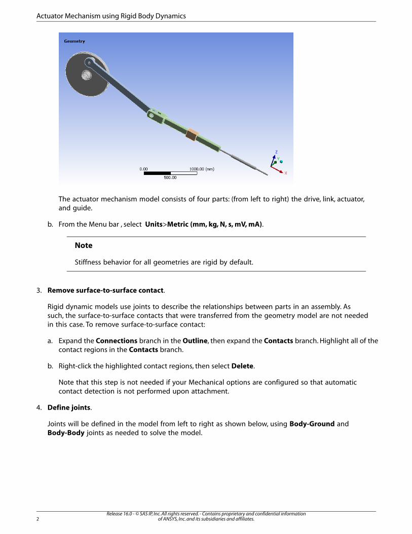
The actuator mechanism model consists of four parts: (from left to right) the drive, link, actuator,and guide.
b. From the Menu bar , select Units>Metric (mm, kg, N, s, mV, mA).
Note
Stiffness behavior for all geometries are rigid by default.
3. Remove surface-to-surface contact.
Rigid dynamic models use joints to describe the relationships between parts in an assembly. Assuch, the surface-to-surface contacts that were transferred from the geometry model are not neededin this case. To remove surface-to-surface contact:
a. Expand the Connections branch in the Outline, then expand the Contacts branch. Highlight all of thecontact regions in the Contacts branch.
b. Right-click the highlighted contact regions, then select Delete.
Note that this step is not needed if your Mechanical options are configured so that automaticcontact detection is not performed upon attachment.
4. Define joints.
Joints will be defined in the model from left to right as shown below, using Body-Ground andBody-Body joints as needed to solve the model.
Release 16.0 - © SAS IP, Inc. All rights reserved. - Contains proprietary and confidential informationof ANSYS, Inc. and its subsidiaries and affiliates.2
Actuator Mechanism using Rigid Body Dynamics

Prior to defining joints, it is useful to select the Body Views button in the Connections toolbar. TheBody Views button splits the graphics window into three sections: the main window, the referencebody window, and the mobile body window. Each window can be manipulated independently. Thismakes it easier to select desired regions on the model when scoping joints.
To define joints:
a. Select the drive pin face and link center hole face as shown below, then select Body-Body>Revolutein the Connections toolbar.
3Release 16.0 - © SAS IP, Inc. All rights reserved. - Contains proprietary and confidential information
of ANSYS, Inc. and its subsidiaries and affiliates.

b. Select the drive center hole face as shown below, then select Body-Ground>Revolute in the Connec-tions toolbar.
c. Select the link face and actuator center hole face as shown below, then select Body-Body>Revolutein the Connections toolbar.
d. Select the actuator face and the guide face as shown below, then select Body-Body>Translational inthe Connections toolbar.
Release 16.0 - © SAS IP, Inc. All rights reserved. - Contains proprietary and confidential informationof ANSYS, Inc. and its subsidiaries and affiliates.4
Actuator Mechanism using Rigid Body Dynamics

e. Select the guide top face as shown below, then select Body-Ground>Fixed in the Connections toolbar.
5. Define joint coordinate systems.
The coordinate systems for each new joint must be properly defined to ensure correct joint motion.Realign each joint coordinate system so that they match the corresponding systems pictured in step4. To specify a joint coordinate system:
a. In the Outline, highlight a joint in the Joints branch.
5Release 16.0 - © SAS IP, Inc. All rights reserved. - Contains proprietary and confidential information
of ANSYS, Inc. and its subsidiaries and affiliates.
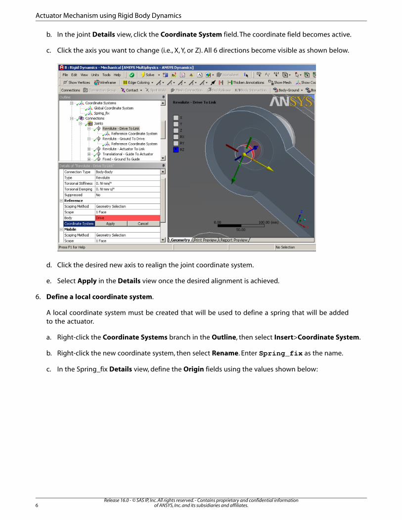
b. In the joint Details view, click the Coordinate System field. The coordinate field becomes active.
c. Click the axis you want to change (i.e., X, Y, or Z). All 6 directions become visible as shown below.
d. Click the desired new axis to realign the joint coordinate system.
e. Select Apply in the Details view once the desired alignment is achieved.
6. Define a local coordinate system.
A local coordinate system must be created that will be used to define a spring that will be addedto the actuator.
a. Right-click the Coordinate Systems branch in the Outline, then select Insert>Coordinate System.
b. Right-click the new coordinate system, then select Rename. Enter Spring_fix as the name.
c. In the Spring_fix Details view, define the Origin fields using the values shown below:
Release 16.0 - © SAS IP, Inc. All rights reserved. - Contains proprietary and confidential informationof ANSYS, Inc. and its subsidiaries and affiliates.6
Actuator Mechanism using Rigid Body Dynamics

7. Add a spring to the actuator.
a. Select the bottom face of the actuator as shown below, then select Body-Ground>Spring in theConnections toolbar.
b. In the Reference section of the spring Details view, set the Coordinate System to Spring_fix.
c. In the Definition section of the spring Details view, specify:
Longitudinal Stiffness = 0.005 N/mmLongitudinal Damping = 0.01 N*s/mm
7Release 16.0 - © SAS IP, Inc. All rights reserved. - Contains proprietary and confidential information
of ANSYS, Inc. and its subsidiaries and affiliates.

8. Define analysis settings.
To define the length of the analysis:
a. Select the Analysis Settings branch in the Outline.
b. In the Analysis Settings Details view, specify Step End Time = 60. s
9. Define a joint load.
A joint load must be defined to apply a kinematic driving condition to the joint object. To define ajoint load:
a. Right-click the Transient branch in the Outline, then select Insert>Joint Load.
b. In the Joint Load Details view, specify:
Joint = Revolute - Ground To DriveType = MomentMagnitude = Tabular (Time)
Graph and Tabular Data windows will appear.
c. In the Tabular Data window, specify that Moment = 5000 at Time = 60, as shown below.
10. Prepare the solution
Release 16.0 - © SAS IP, Inc. All rights reserved. - Contains proprietary and confidential informationof ANSYS, Inc. and its subsidiaries and affiliates.8
Actuator Mechanism using Rigid Body Dynamics
a. Select Solution in the Outline, then select Deformation>Total in the Solution toolbar.
b. In the Outline, click and drag the link to actuator revolute joint to the Solution branch. Joint Probewill appear under the Solution branch.
This is a shortcut for creating a joint probe that is already scoped to the joint in question. Becausewe want to find the forces acting on this joint, the default settings in the details of the jointprobe are used.
c. Click the Solve button in the main toolbar.
11. Analyze the results
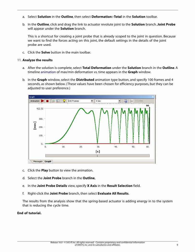
a. After the solution is complete, select Total Deformation under the Solution branch in the Outline. Atimeline animation of max/min deformation vs. time appears in the Graph window.
b. In the Graph window, select the Distributed animation type button, and specify 100 frames and 4seconds, as shown below. (These values have been chosen for efficiency purposes, but they can beadjusted to user preference.)
c. Click the Play button to view the animation.
d. Select the Joint Probe branch in the Outline,
e. In the Joint Probe Details view, specify X Axis in the Result Selection field.
f. Right-click the Joint Probe branch, then select Evaluate All Results.
The results from the analysis show that the spring-based actuator is adding energy in to the systemthat is reducing the cycle time.
End of tutorial.
9Release 16.0 - © SAS IP, Inc. All rights reserved. - Contains proprietary and confidential information
of ANSYS, Inc. and its subsidiaries and affiliates.

Release 16.0 - © SAS IP, Inc. All rights reserved. - Contains proprietary and confidential informationof ANSYS, Inc. and its subsidiaries and affiliates.10
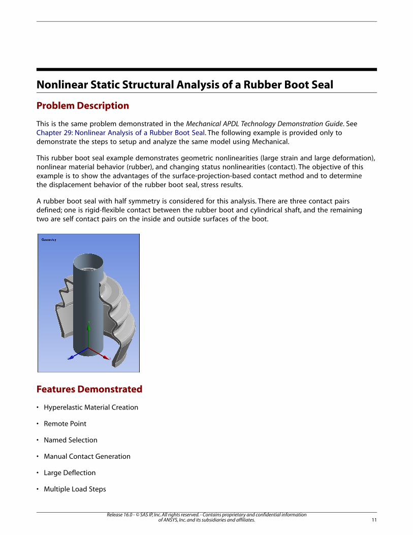
Nonlinear Static Structural Analysis of a Rubber Boot Seal
Problem Description
This is the same problem demonstrated in the Mechanical APDL Technology Demonstration Guide. SeeChapter 29: Nonlinear Analysis of a Rubber Boot Seal. The following example is provided only todemonstrate the steps to setup and analyze the same model using Mechanical.
This rubber boot seal example demonstrates geometric nonlinearities (large strain and large deformation),nonlinear material behavior (rubber), and changing status nonlinearities (contact). The objective of thisexample is to show the advantages of the surface-projection-based contact method and to determinethe displacement behavior of the rubber boot seal, stress results.
A rubber boot seal with half symmetry is considered for this analysis. There are three contact pairsdefined; one is rigid-flexible contact between the rubber boot and cylindrical shaft, and the remainingtwo are self contact pairs on the inside and outside surfaces of the boot.
Features Demonstrated
• Hyperelastic Material Creation
• Remote Point
• Named Selection
• Manual Contact Generation
• Large Deflection
• Multiple Load Steps
11Release 16.0 - © SAS IP, Inc. All rights reserved. - Contains proprietary and confidential information
of ANSYS, Inc. and its subsidiaries and affiliates.

• Nodal Contacts
Setting Up the Analysis System
1. Create a Static Structural analysis system.
a. Start ANSYS Workbench.
b. On the Workbench Project page, drag a Static Structural system from the Toolbox to the ProjectSchematic.
2. Create Materials.
For this tutorial, we are going to create a material to use during the analysis.
a. In the Static Structural schematic, right-click the Engineering Data cell and choose Edit. The EngineeringData tab opens. Structural Steel is the default material.
b. From the Engineering Data tab, place your cursor in the Click here to add new material field and thenenter "Rubber Material".
Release 16.0 - © SAS IP, Inc. All rights reserved. - Contains proprietary and confidential informationof ANSYS, Inc. and its subsidiaries and affiliates.12
Nonlinear Static Structural Analysis of a Rubber Boot Seal
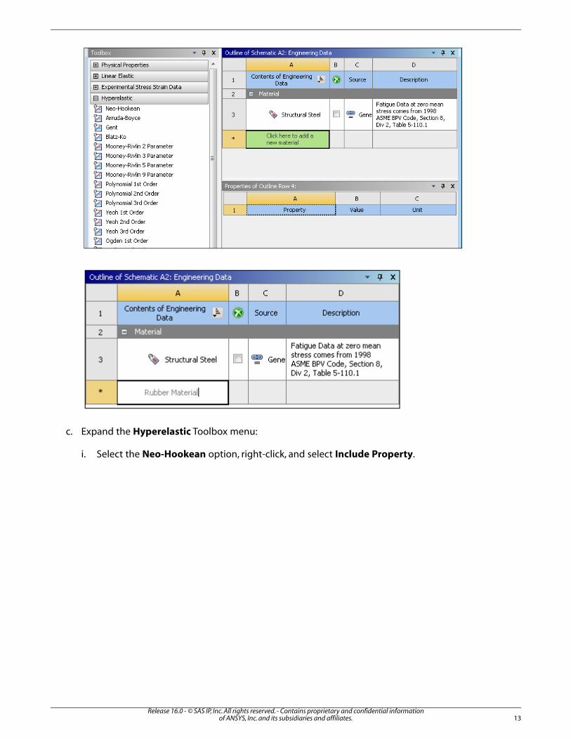
c. Expand the Hyperelastic Toolbox menu:
i. Select the Neo-Hookean option, right-click, and select Include Property.
13Release 16.0 - © SAS IP, Inc. All rights reserved. - Contains proprietary and confidential information
of ANSYS, Inc. and its subsidiaries and affiliates.
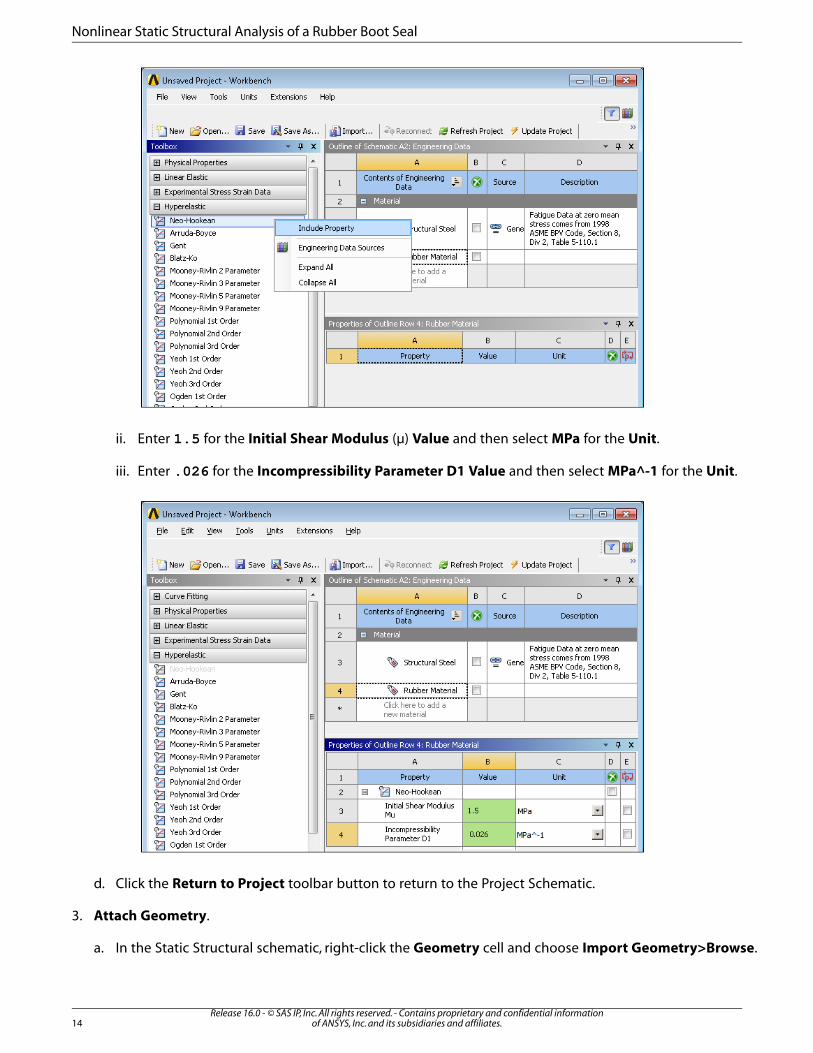
ii. Enter 1.5 for the Initial Shear Modulus (μ) Value and then select MPa for the Unit.
iii. Enter .026 for the Incompressibility Parameter D1 Value and then select MPa^-1 for the Unit.
d. Click the Return to Project toolbar button to return to the Project Schematic.
3. Attach Geometry.
a. In the Static Structural schematic, right-click the Geometry cell and choose Import Geometry>Browse.
Release 16.0 - © SAS IP, Inc. All rights reserved. - Contains proprietary and confidential informationof ANSYS, Inc. and its subsidiaries and affiliates.14
Nonlinear Static Structural Analysis of a Rubber Boot Seal
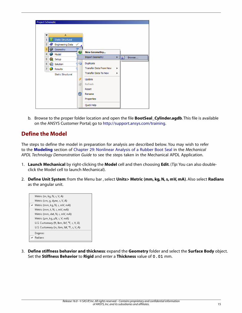
b. Browse to the proper folder location and open the file BootSeal_Cylinder.agdb. This file is availableon the ANSYS Customer Portal; go to http://support.ansys.com/training.
Define the Model
The steps to define the model in preparation for analysis are described below. You may wish to referto the Modeling section of Chapter 29: Nonlinear Analysis of a Rubber Boot Seal in the MechanicalAPDL Technology Demonstration Guide to see the steps taken in the Mechanical APDL Application.
1. Launch Mechanical by right-clicking the Model cell and then choosing Edit. (Tip: You can also double-click the Model cell to launch Mechanical).
2. Define Unit System: from the Menu bar , select Units> Metric (mm, kg, N, s, mV, mA). Also select Radiansas the angular unit.
3. Define stiffness behavior and thickness: expand the Geometry folder and select the Surface Body object.Set the Stiffness Behavior to Rigid and enter a Thickness value of 0.01 mm.
15Release 16.0 - © SAS IP, Inc. All rights reserved. - Contains proprietary and confidential information
of ANSYS, Inc. and its subsidiaries and affiliates.

4. In the Geometry folder, select the Solid geometry object. In the Details under the Material category, openthe Assignment property drop-down list and select Rubber Material.
5. Create a Cylindrical Coordinate System: Right-click the Coordinate Systems folder and select Insert>Co-ordinate System. Highlight the new Coordinate System object, right-click, and rename it to "CylindricalCoordinate System".
Specify properties of the Cylindrical Coordinate System:
a. Under the Details view Definition category, change Type to Cylindrical and Coordinate System toManual.
b. Under the Origin group, change the Define By property to Global Coordinates.
Release 16.0 - © SAS IP, Inc. All rights reserved. - Contains proprietary and confidential informationof ANSYS, Inc. and its subsidiaries and affiliates.16
Nonlinear Static Structural Analysis of a Rubber Boot Seal
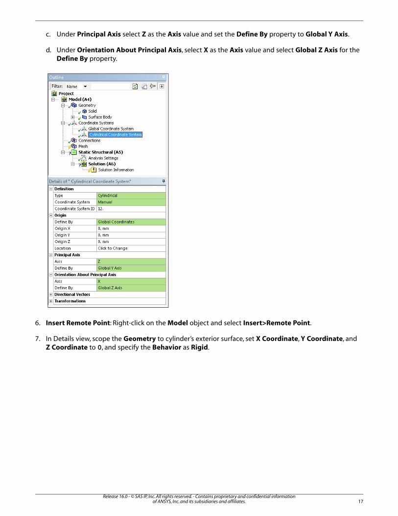
c. Under Principal Axis select Z as the Axis value and set the Define By property to Global Y Axis.
d. Under Orientation About Principal Axis, select X as the Axis value and select Global Z Axis for theDefine By property.
6. Insert Remote Point: Right-click on the Model object and select Insert>Remote Point.
7. In Details view, scope the Geometry to cylinder’s exterior surface, set X Coordinate, Y Coordinate, andZ Coordinate to 0, and specify the Behavior as Rigid.
17Release 16.0 - © SAS IP, Inc. All rights reserved. - Contains proprietary and confidential information
of ANSYS, Inc. and its subsidiaries and affiliates.

8. Define Named Selections:
a. Right-click on the Model object and select Insert>Named Selection.
b. Select the exterior surface of the cylinder, Apply it as the Geometry, right-click, and Rename it toCylinder_Outer_Surface.
c. Right-click on the Surface Body object under the Geometry folder and select Hide Body. This stepeases the selection of the boot’s inner surfaces.
Release 16.0 - © SAS IP, Inc. All rights reserved. - Contains proprietary and confidential informationof ANSYS, Inc. and its subsidiaries and affiliates.18
Nonlinear Static Structural Analysis of a Rubber Boot Seal

d. Highlight the Named Selection object and select Insert>Named Selection.
e. Select all of the inner faces of the boot seal as illustrated below and scope the faces as the Geometryselection. Make sure that the Geometry property indicates that 24 Faces are selected.
Press the Ctrl key to select multiple surfaces individually or you can hold down the mouse buttonand methodically drag the cursor across all of the interior surfaces. Note that the status bar atthe bottom of the graphics window displays the number of selected surfaces (highlighted ingreen in the following image).
f. Right-click the new Selection object and Rename it to Boot_Seal_Inner_Surfaces.
19Release 16.0 - © SAS IP, Inc. All rights reserved. - Contains proprietary and confidential information
of ANSYS, Inc. and its subsidiaries and affiliates.

g. Again highlight the Named Selection object and select Insert>Named Selection.
h. Reorient your model and select all of the outer faces of the boot seal as illustrated below and scopethe faces as the Geometry selection. Make sure that the Geometry property indicates that 27 Facesare selected.
The selection process is the same. Press the Ctrl key to select multiple surfaces individually oryou can hold down the mouse button and methodically drag the cursor across all of the surfaces(except the top surface of the boot).
Release 16.0 - © SAS IP, Inc. All rights reserved. - Contains proprietary and confidential informationof ANSYS, Inc. and its subsidiaries and affiliates.20
Nonlinear Static Structural Analysis of a Rubber Boot Seal
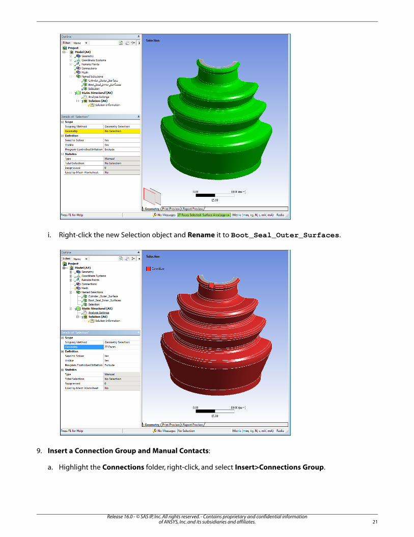
i. Right-click the new Selection object and Rename it to Boot_Seal_Outer_Surfaces.
9. Insert a Connection Group and Manual Contacts:
a. Highlight the Connections folder, right-click, and select Insert>Connections Group.
21Release 16.0 - © SAS IP, Inc. All rights reserved. - Contains proprietary and confidential information
of ANSYS, Inc. and its subsidiaries and affiliates.
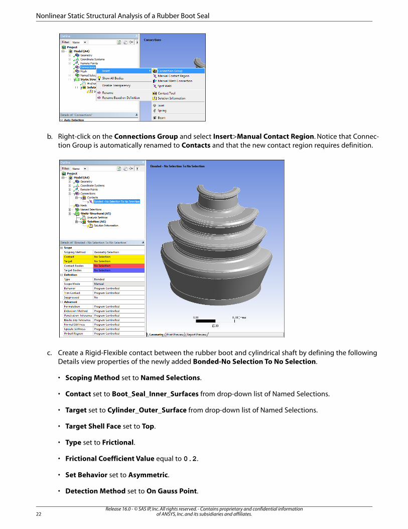
b. Right-click on the Connections Group and select Insert>Manual Contact Region. Notice that Connec-tion Group is automatically renamed to Contacts and that the new contact region requires definition.
c. Create a Rigid-Flexible contact between the rubber boot and cylindrical shaft by defining the followingDetails view properties of the newly added Bonded-No Selection To No Selection.
• Scoping Method set to Named Selections.
• Contact set to Boot_Seal_Inner_Surfaces from drop-down list of Named Selections.
• Target set to Cylinder_Outer_Surface from drop-down list of Named Selections.
• Target Shell Face set to Top.
• Type set to Frictional.
• Frictional Coefficient Value equal to 0.2.
• Set Behavior set to Asymmetric.
• Detection Method set to On Gauss Point.
Release 16.0 - © SAS IP, Inc. All rights reserved. - Contains proprietary and confidential informationof ANSYS, Inc. and its subsidiaries and affiliates.22
Nonlinear Static Structural Analysis of a Rubber Boot Seal

• Interface Treatment set to Add Offset, Ramped Effects.
23Release 16.0 - © SAS IP, Inc. All rights reserved. - Contains proprietary and confidential information
of ANSYS, Inc. and its subsidiaries and affiliates.
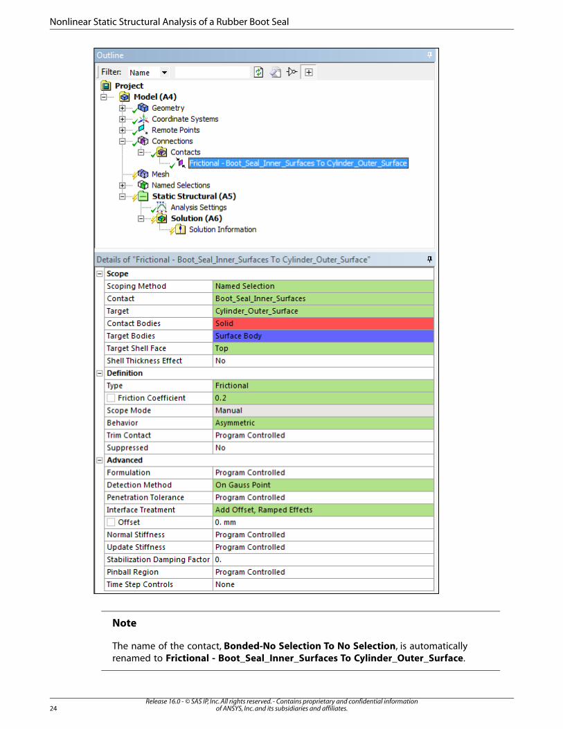
Note
The name of the contact, Bonded-No Selection To No Selection, is automaticallyrenamed to Frictional - Boot_Seal_Inner_Surfaces To Cylinder_Outer_Surface.
Release 16.0 - © SAS IP, Inc. All rights reserved. - Contains proprietary and confidential informationof ANSYS, Inc. and its subsidiaries and affiliates.24
Nonlinear Static Structural Analysis of a Rubber Boot Seal
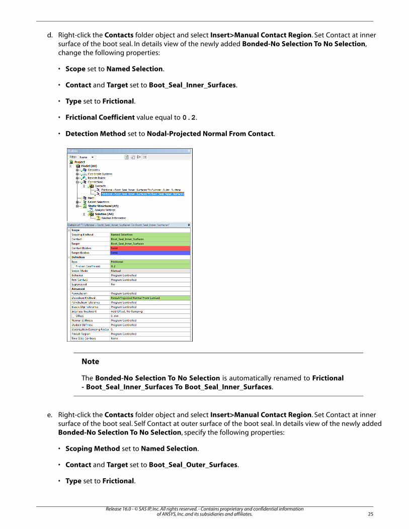
d. Right-click the Contacts folder object and select Insert>Manual Contact Region. Set Contact at innersurface of the boot seal. In details view of the newly added Bonded-No Selection To No Selection,change the following properties:
• Scope set to Named Selection.
• Contact and Target set to Boot_Seal_Inner_Surfaces.
• Type set to Frictional.
• Frictional Coefficient value equal to 0.2.
• Detection Method set to Nodal-Projected Normal From Contact.
Note
The Bonded-No Selection To No Selection is automatically renamed to Frictional- Boot_Seal_Inner_Surfaces To Boot_Seal_Inner_Surfaces.
e. Right-click the Contacts folder object and select Insert>Manual Contact Region. Set Contact at innersurface of the boot seal. Self Contact at outer surface of the boot seal. In details view of the newly addedBonded-No Selection To No Selection, specify the following properties:
• Scoping Method set to Named Selection.
• Contact and Target set to Boot_Seal_Outer_Surfaces.
• Type set to Frictional.
25Release 16.0 - © SAS IP, Inc. All rights reserved. - Contains proprietary and confidential information
of ANSYS, Inc. and its subsidiaries and affiliates.

• Frictional Coefficient Value equal to 0.2.
• Detection Method set to Nodal-Projected Normal From Contact.
Note
Bonded-No Selection To No Selection is automatically renamed to Frictional -Boot_Seal_Outer_Surfaces To Boot_Seal_Outer_Surfaces.
Analysis Settings
The problem is solved in three load steps, which include:
• Initial interference between the cylinder and boot.
• Vertical displacement of the cylinder (axial compression in the rubber boot).
• Rotation of the cylinder (bending of the rubber boot).
Load steps are specified through the properties of the Analysis Settings object.
1. Highlight the Analysis Settings object.
2. Define the following properties:
• Number of Steps equals 3.
• Auto Time Stepping set to On (from Program Controlled).
• Define By set to Substeps.
Release 16.0 - © SAS IP, Inc. All rights reserved. - Contains proprietary and confidential informationof ANSYS, Inc. and its subsidiaries and affiliates.26
Nonlinear Static Structural Analysis of a Rubber Boot Seal

• Initial Substeps and Minimum Substeps set to 5.
• Maximum Substeps set to 1000.
• Large Deflection set to On.
3. For the second load step, define the properties as follows:
• Current Step Number to 2.
• Auto Time Stepping set to On (from Program Controlled).
• Initial Substeps and Minimum Substeps set to 10.
• Maximum Substeps set to 1000.
4. For the third load step, define the properties as follows:
• Current Step Number to 3.
• Auto Time Stepping set to On (from Program Controlled).
• Initial Substeps and Minimum Substeps set to 20.
• Maximum Substeps set to 1000.
27Release 16.0 - © SAS IP, Inc. All rights reserved. - Contains proprietary and confidential information
of ANSYS, Inc. and its subsidiaries and affiliates.
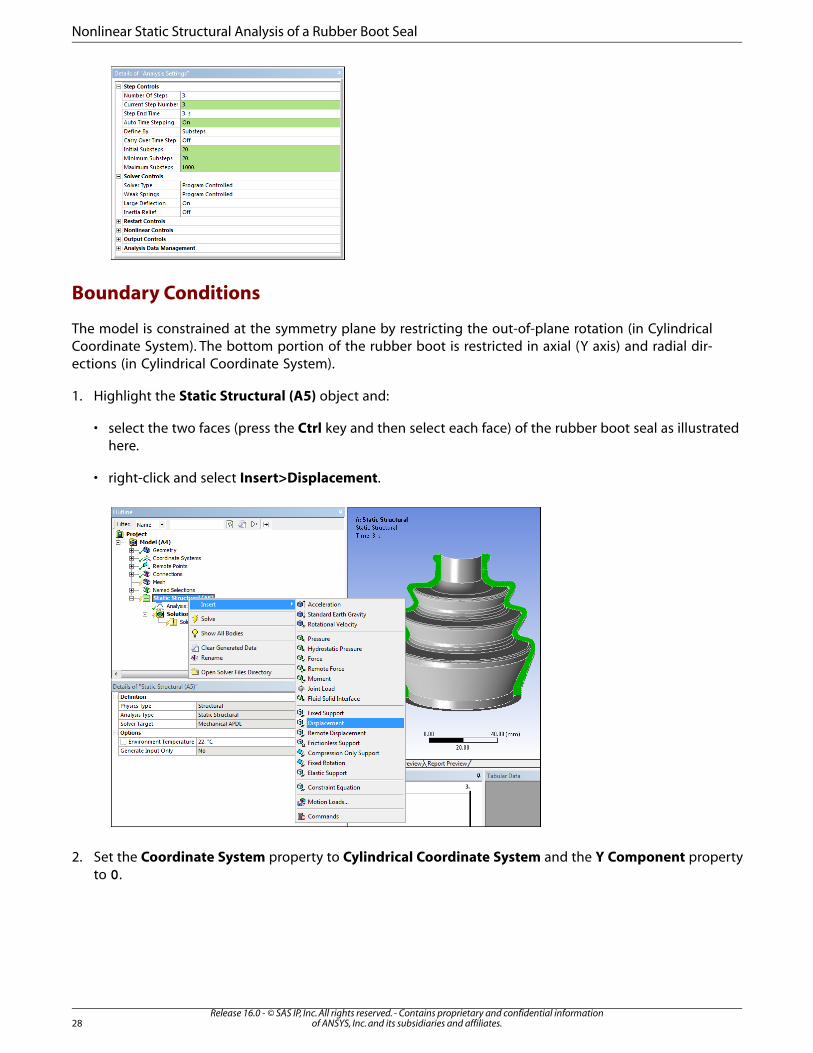
Boundary Conditions
The model is constrained at the symmetry plane by restricting the out-of-plane rotation (in CylindricalCoordinate System). The bottom portion of the rubber boot is restricted in axial (Y axis) and radial dir-ections (in Cylindrical Coordinate System).
1. Highlight the Static Structural (A5) object and:
• select the two faces (press the Ctrl key and then select each face) of the rubber boot seal as illustratedhere.
• right-click and select Insert>Displacement.
2. Set the Coordinate System property to Cylindrical Coordinate System and the Y Component propertyto 0.
Release 16.0 - © SAS IP, Inc. All rights reserved. - Contains proprietary and confidential informationof ANSYS, Inc. and its subsidiaries and affiliates.28
Nonlinear Static Structural Analysis of a Rubber Boot Seal

3. Highlight the Static Structural (A5) object and select the face illustrated here. Insert another Displacementand set the Y Component to 0 (Coordinate System should equal Global Coordinate System).
4. Insert another Displacement scoped as illustrated here and set the Coordinate System property to Cyl-indrical Coordinate System and the X Component property to 0.
29Release 16.0 - © SAS IP, Inc. All rights reserved. - Contains proprietary and confidential information
of ANSYS, Inc. and its subsidiaries and affiliates.
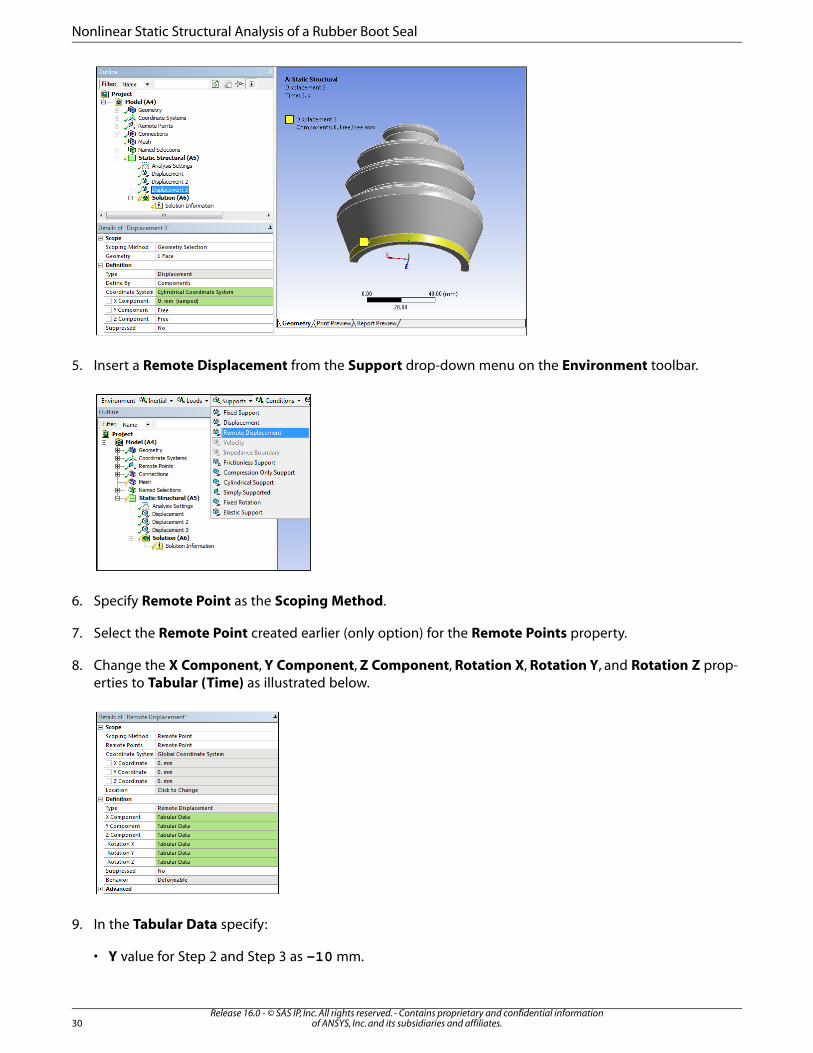
5. Insert a Remote Displacement from the Support drop-down menu on the Environment toolbar.
6. Specify Remote Point as the Scoping Method.
7. Select the Remote Point created earlier (only option) for the Remote Points property.
8. Change the X Component, Y Component, Z Component, Rotation X, Rotation Y, and Rotation Z prop-erties to Tabular (Time) as illustrated below.
9. In the Tabular Data specify:
• Y value for Step 2 and Step 3 as -10 mm.
Release 16.0 - © SAS IP, Inc. All rights reserved. - Contains proprietary and confidential informationof ANSYS, Inc. and its subsidiaries and affiliates.30
Nonlinear Static Structural Analysis of a Rubber Boot Seal
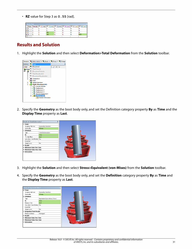
• RZ value for Step 3 as 0.55 [rad].
Results and Solution
1. Highlight the Solution and then select Deformation>Total Deformation from the Solution toolbar.
2. Specify the Geometry as the boot body only, and set the Definition category property By as Time and theDisplay Time property as Last.
3. Highlight the Solution and then select Stress>Equivalent (von-Mises) from the Solution toolbar.
4. Specify the Geometry as the boot body only, and set the Definition category property By as Time andthe Display Time property as Last.
31Release 16.0 - © SAS IP, Inc. All rights reserved. - Contains proprietary and confidential information
of ANSYS, Inc. and its subsidiaries and affiliates.
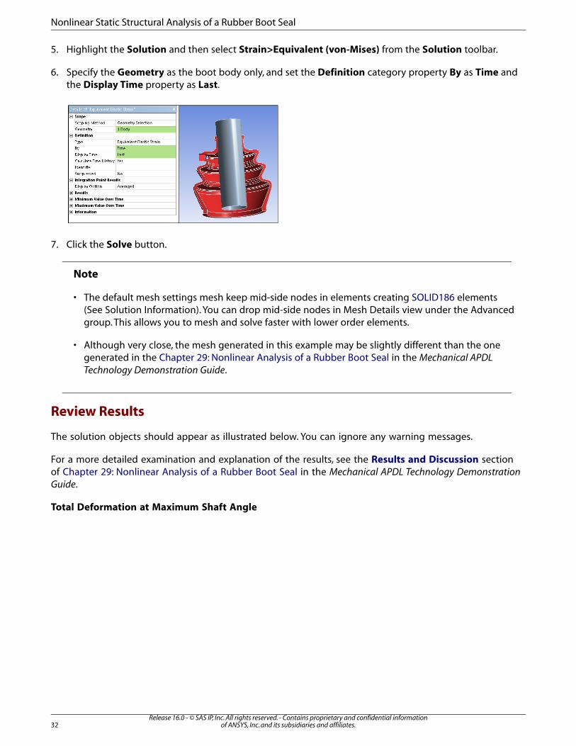
5. Highlight the Solution and then select Strain>Equivalent (von-Mises) from the Solution toolbar.
6. Specify the Geometry as the boot body only, and set the Definition category property By as Time andthe Display Time property as Last.
7. Click the Solve button.
Note
• The default mesh settings mesh keep mid-side nodes in elements creating SOLID186 elements(See Solution Information). You can drop mid-side nodes in Mesh Details view under the Advancedgroup. This allows you to mesh and solve faster with lower order elements.
• Although very close, the mesh generated in this example may be slightly different than the onegenerated in the Chapter 29: Nonlinear Analysis of a Rubber Boot Seal in the Mechanical APDLTechnology Demonstration Guide.
Review Results
The solution objects should appear as illustrated below. You can ignore any warning messages.
For a more detailed examination and explanation of the results, see the Results and Discussion sectionof Chapter 29: Nonlinear Analysis of a Rubber Boot Seal in the Mechanical APDL Technology DemonstrationGuide.
Total Deformation at Maximum Shaft Angle
Release 16.0 - © SAS IP, Inc. All rights reserved. - Contains proprietary and confidential informationof ANSYS, Inc. and its subsidiaries and affiliates.32
Nonlinear Static Structural Analysis of a Rubber Boot Seal
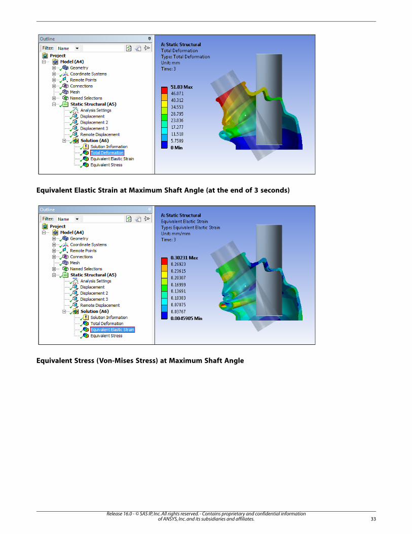
Equivalent Elastic Strain at Maximum Shaft Angle (at the end of 3 seconds)
Equivalent Stress (Von-Mises Stress) at Maximum Shaft Angle
33Release 16.0 - © SAS IP, Inc. All rights reserved. - Contains proprietary and confidential information
of ANSYS, Inc. and its subsidiaries and affiliates.

End of tutorial.
Release 16.0 - © SAS IP, Inc. All rights reserved. - Contains proprietary and confidential informationof ANSYS, Inc. and its subsidiaries and affiliates.34
Nonlinear Static Structural Analysis of a Rubber Boot Seal
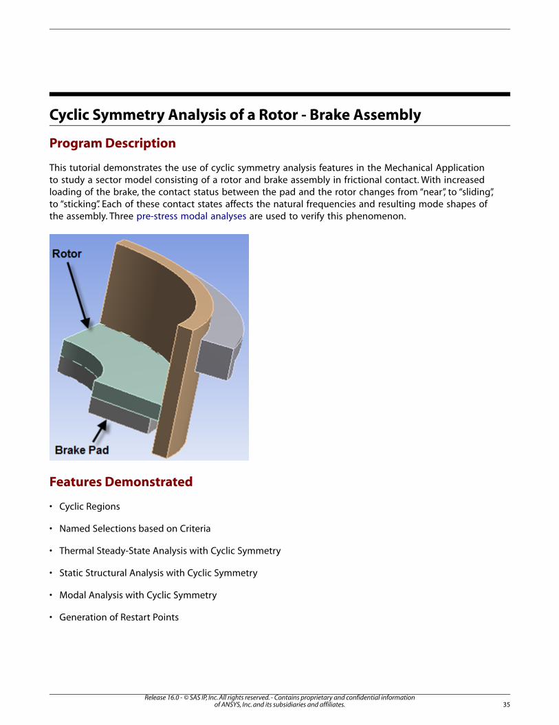
Cyclic Symmetry Analysis of a Rotor - Brake Assembly
Program Description
This tutorial demonstrates the use of cyclic symmetry analysis features in the Mechanical Applicationto study a sector model consisting of a rotor and brake assembly in frictional contact. With increasedloading of the brake, the contact status between the pad and the rotor changes from “near”, to “sliding”,to “sticking”. Each of these contact states affects the natural frequencies and resulting mode shapes ofthe assembly. Three pre-stress modal analyses are used to verify this phenomenon.
Features Demonstrated
• Cyclic Regions
• Named Selections based on Criteria
• Thermal Steady-State Analysis with Cyclic Symmetry
• Static Structural Analysis with Cyclic Symmetry
• Modal Analysis with Cyclic Symmetry
• Generation of Restart Points
35Release 16.0 - © SAS IP, Inc. All rights reserved. - Contains proprietary and confidential information
of ANSYS, Inc. and its subsidiaries and affiliates.
• Modal Analysis with Nonlinear Prestress (Linear Perturbation)
Note
The procedural steps in this tutorial assume that you are familiar with basic navigationtechniques within the Mechanical application. If you are new to using the application, considerrunning the tutorial: “Steady-State and Transient Thermal Analysis of a Circuit Board” beforeattempting to run this tutorial.
Analysis System Layout
We will tour the different analysis systems that can leverage cyclic symmetry functionality. These comprisethermal, static structural and modal analyses:
• A steady-state thermal analysis will be used to calculate the temperature distribution for the evaluation ofany temperature-dependent material properties or thermal expansions in subsequent analyses.
• A nonlinear static structural analysis is configured to represent the mechanical loading of the brake ontothe rotor. Nonlinearities from large deformation and changes in contact status are included.
• Modal analyses, each at different stages of frictional contact status, are established to compare the free vi-bration responses of the model.
1. Create the analysis systems.
You need to establish a static structural analysis that is linked to a steady-state thermal analysis,then establish three modal analyses that are linked to the static structural analysis.
a. Start ANSYS Workbench.
b. From the Toolbox, drag a Steady-State Thermal system onto the Project Schematic.
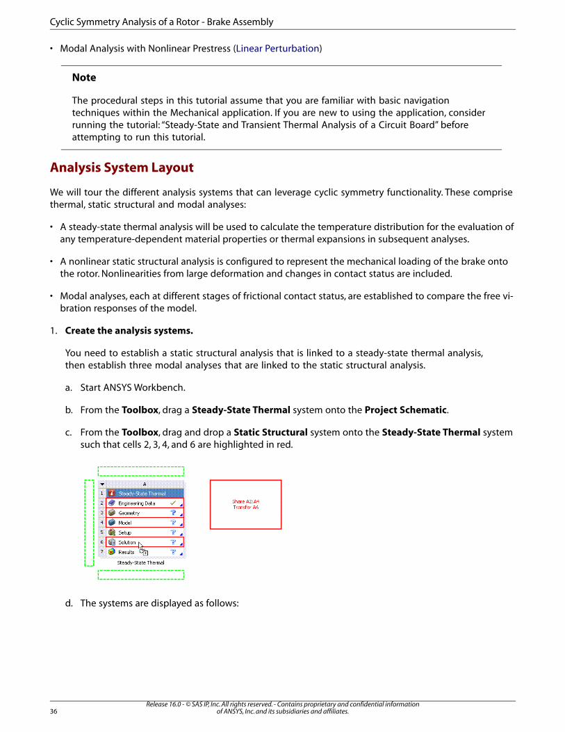
c. From the Toolbox, drag and drop a Static Structural system onto the Steady-State Thermal systemsuch that cells 2, 3, 4, and 6 are highlighted in red.
d. The systems are displayed as follows:
Release 16.0 - © SAS IP, Inc. All rights reserved. - Contains proprietary and confidential informationof ANSYS, Inc. and its subsidiaries and affiliates.36
Cyclic Symmetry Analysis of a Rotor - Brake Assembly

e. To measure the free vibration response, go to the Toolbox, drag and drop a Modal system onto theStatic Structural system such that cells 2, 3, 4, and 6 are highlighted in red.
f. Repeat step e two more times to complete adding the remaining analysis systems. The layout of theanalysis systems and interconnections in the Project Schematic should appear as shown below.
2. Assign materials.
Accept Structural Steel (typically the default material) for the model.
37Release 16.0 - © SAS IP, Inc. All rights reserved. - Contains proprietary and confidential information
of ANSYS, Inc. and its subsidiaries and affiliates.

a. In the Steady-State Thermal schematic, right-click the Engineering Data cell and choose Edit.... TheEngineering Data tab opens and displays Structural Steel as the default material.
b. Click the Return to Project toolbar button.
3. Attach geometry.
a. In the Steady-State Thermal schematic, right-click the Geometry cell, and then choose Import Geo-metry.
b. Browse to open the file Rotor_Brake.agdb. This file is available on the ANSYS Customer Portal; goto http://support.ansys.com/training.
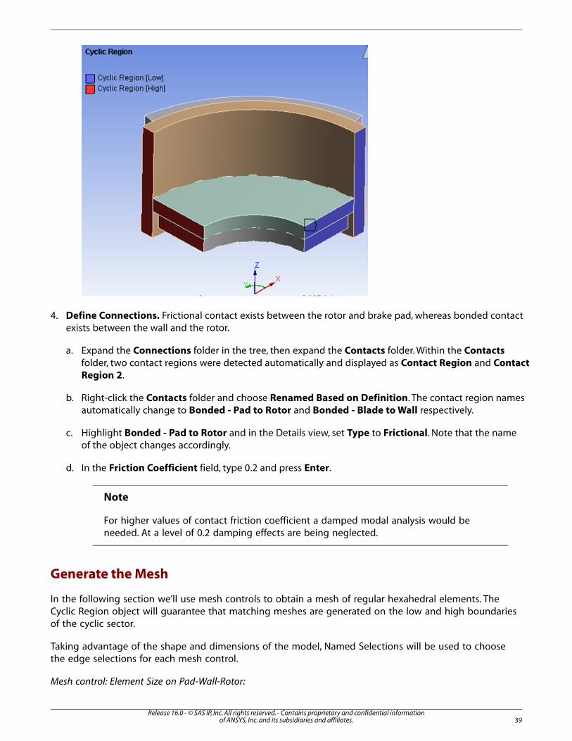
Define the Cyclic Symmetry Model
We now specify the cyclic symmetry for our quarter sector model (N = 4, 90 degrees) and prepare othergeneral aspects of modeling in the Mechanical application. To setup a cyclic symmetry analysis, Mech-anical uses a Cyclic Region object. This object requires selection of the sector boundaries, togetherwith a cylindrical coordinate system whose Z axis is colinear with the axis of symmetry, and whose Yaxis distinguishes the low and high boundaries.
1. Enter the Mechanical Application and set unit systems.
a. In the Steady-State Thermal schematic, right-click the Model cell, and then choose Edit.... TheMechanical Application opens and displays the model.
b. From the Menu bar , choose Units> Metric (mm, kg, N, s, mV, mA) .
2. Define the Coordinate System to specify the axis of symmetry.
a. Right-click Coordinate Systems in the tree and choose Insert> Coordinate System.
b. In the Details view of the newly-created Coordinate System, set Type to Cylindrical and Define Byto Global Coordinates.
3. Define the Cyclic Region object.
a. Right-click Model in the tree and choose Insert> Symmetry.
b. Right-click Symmetry and choose Insert> Cyclic Region. The direction of the Y-axis should be compat-ible with the selection of low and high boundaries. The low boundary is designated as the one with alower value of Y or azimuth.
c. Select the three faces that have lower azimuth for the low boundary. These faces are highlighted inblue in the figure below.
d. Select the three matching faces on the opposite end of the sector for the high boundary. These facesare highlighted in red in the figure below
Release 16.0 - © SAS IP, Inc. All rights reserved. - Contains proprietary and confidential informationof ANSYS, Inc. and its subsidiaries and affiliates.38
Cyclic Symmetry Analysis of a Rotor - Brake Assembly
4. Define Connections. Frictional contact exists between the rotor and brake pad, whereas bonded contactexists between the wall and the rotor.
a. Expand the Connections folder in the tree, then expand the Contacts folder. Within the Contactsfolder, two contact regions were detected automatically and displayed as Contact Region and ContactRegion 2.
b. Right-click the Contacts folder and choose Renamed Based on Definition. The contact region namesautomatically change to Bonded - Pad to Rotor and Bonded - Blade to Wall respectively.
c. Highlight Bonded - Pad to Rotor and in the Details view, set Type to Frictional. Note that the nameof the object changes accordingly.
d. In the Friction Coefficient field, type 0.2 and press Enter.
Note
For higher values of contact friction coefficient a damped modal analysis would beneeded. At a level of 0.2 damping effects are being neglected.
Generate the Mesh
In the following section we’ll use mesh controls to obtain a mesh of regular hexahedral elements. TheCyclic Region object will guarantee that matching meshes are generated on the low and high boundariesof the cyclic sector.
Taking advantage of the shape and dimensions of the model, Named Selections will be used to choosethe edge selections for each mesh control.
Mesh control: Element Size on Pad-Wall-Rotor:
39Release 16.0 - © SAS IP, Inc. All rights reserved. - Contains proprietary and confidential information
of ANSYS, Inc. and its subsidiaries and affiliates.

1. Create a Named Selection for this Mesh Control.
a. Right-click on Model and choose Insert> Named Selection.
b. Highlight the Selection object, and set Scoping Method to Worksheet.
c. Program the Worksheet, as shown below, to select the edges at 90 degrees of azimuth in the cylindricalcoordinate system, keeping those in the z-axis range [1mm, 6 mm] (to remove the thickness of thewall). To add rows to the Worksheet, right-click in the table and select the option from the flyout menus.
d. Click the Generate button. You should see 11 edges.
e. Rename the object to Edges for Wall Rotor Pad Sector Boundary. The selection should display asfollows:.
Note
It may be useful to undock the Worksheet window and tile it with the Geometryview as shown above.
2. Insert a Mesh Sizing control.
a. Right-click on Mesh and choose Insert> Sizing.
b. Set Scoping Method to Named Selection.
c. Choose the named selection defined in the previous step.
Release 16.0 - © SAS IP, Inc. All rights reserved. - Contains proprietary and confidential informationof ANSYS, Inc. and its subsidiaries and affiliates.40
Cyclic Symmetry Analysis of a Rotor - Brake Assembly

d. Set its Element Size to 0.5 mm.
e. Set Behavior to Soft.
Mesh control: Number of Divisions on Pad-Rotor:
1. Create a Named Selection to pick the circular edges in the orifice of the pad and rotor.
This Named Selection will pick the circular edges in the orifice of the pad and rotor, which is withina radius of 5 mm.
a. Right-click on Model and choose Insert> Named Selection.
b. Highlight the Selection object, and set Scoping Method to Worksheet.
c. Rename the object to Edges for Rotor Pad Orifice.
d. Program the Worksheet, as shown below.
e. Click the Generate button. You should see 4 edges.
2. Insert a Mesh Sizing Control as before to select this Named Selection.
a. Right-click on Mesh and choose Insert> Sizing.
b. Set Scoping Method to Named Selection.
c. Choose the named selection defined in the previous step.
d. Set its Type to Number of Divisions and specify 9.
e. Set Behavior to Hard.
Mesh control: Element Size on Wall-Blade
1. Create a Named Selection object to pick the thicknesses of the Wall and Blade.
a. Right-click on Model and choose Insert> Named Selection.
b. Highlight the Selection object, and set Scoping Method to Worksheet.
c. Rename the object to Edges for Wall Blade Thicknesses.
d. Program the Worksheet as shown below.
41Release 16.0 - © SAS IP, Inc. All rights reserved. - Contains proprietary and confidential information
of ANSYS, Inc. and its subsidiaries and affiliates.

e. Click the Generate button. You should see 16 edges.
2. Insert a Mesh Sizing Control as before to select this Named Selection.
a. Right-click on Mesh and choose Insert> Sizing.
b. Set Scoping Method to Named Selection.
c. Choose the named selection defined in the previous step.
d. Set its Element Size to 1 mm.
e. Set Behavior to Hard.
Mesh Control: Number of Divisions on Blade - Longer Edges
1. Create a Named Selection object to pick the longer edges of the Blade.
a. Right-click on Model and choose Insert> Named Selection.
b. Highlight the Selection object, and set Scoping Method to Worksheet.
c. Rename the object to Edges for Blade.
d. Program the Worksheet as shown below.
e. Click the Generate button. You should see 2 edges.
2. Insert a Mesh Sizing Control as before to select this Named Selection.
a. Right-click on Mesh and choose Insert> Sizing.
b. Set Scoping Method to Named Selection.
c. Choose the named selection defined in the previous step.
d. Set its Type to Number of Divisions and specify 14.
e. Set Behavior to Hard.
Mesh Control: Number of Divisions on Blade - Shorter Edges
Release 16.0 - © SAS IP, Inc. All rights reserved. - Contains proprietary and confidential informationof ANSYS, Inc. and its subsidiaries and affiliates.42
Cyclic Symmetry Analysis of a Rotor - Brake Assembly

1. Create a Named Selection object to pick the shorter edges of the Blade.
a. Right-click on Model and choose Insert> Named Selection.
b. Highlight the Selection object, and set Scoping Method to Worksheet.
c. Rename the object to Edges for Blade 2.
d. Program the Worksheet as shown below.
e. Click the Generate button. You should see 2 edges.
2. Insert a Mesh Sizing Control as before to select this Named Selection.
a. Right-click on Mesh and choose Insert> Sizing.
b. Set Scoping Method to Named Selection.
c. Choose the named selection defined in the previous step.
d. Set its Type to Number of Divisions and specify 1.
e. Set Behavior to Hard.
Mesh Control: Method on Pad-Rotor-Wall-Blade
1. Insert a Sweep Method control.
a. Right-click Mesh in the tree and choose Insert> Method.
b. Select all the bodies by choosing Edit> Select All from the toolbar, then click the Apply button.
c. In the Details view, set Method to Sweep.
d. Set Free Face Mesh Type to All Quad.
Generate the Mesh
• For convenience, select all 6 mesh controls defined, right-click and choose Rename Based on Definition.
• Right-click Mesh in the tree and choose Generate Mesh. The mesh should appear as shown below:
43Release 16.0 - © SAS IP, Inc. All rights reserved. - Contains proprietary and confidential information
of ANSYS, Inc. and its subsidiaries and affiliates.

Steady-State Thermal Analysis
We now proceed to define the boundary conditions for a thermal analysis featuring cyclic symmetry.Thermal boundary conditions are prescribed throughout the model while steering clear of the facescomprising the sector boundaries since temperature constraints are already implied there.
1. Define a convection interface.
a. Right-click Steady-State Thermal in the tree and choose Insert> Convection.
b. Select the outer faces of the Wall and the Blade as shown in the figure (8 faces).
c. Specify a Film Coefficient of air by right-clicking on the property and choosing Import TemperatureDependent upon which you choose Stagnant Air - Simplified Case.
2. Insulate the upper and lower faces of the Wall.
• Select the upper and lower faces of the Wall, then right-click and choose Insert> Perfectly Insulated.
3. Apply a temperature load to the Pad and Rotor.
Release 16.0 - © SAS IP, Inc. All rights reserved. - Contains proprietary and confidential informationof ANSYS, Inc. and its subsidiaries and affiliates.44
Cyclic Symmetry Analysis of a Rotor - Brake Assembly

a. Select the remaining faces on the assembly on the Pad and the Rotor, then right-click and choose Insert>Temperature. Exclude any faces on the sector boundaries or in the frictional contact.
b. Type 100°C as the Magnitude and press Enter.
4. Solve and review the temperature distribution.
a. Right-click Solution under Steady-State Thermal and choose Insert> Thermal> Temperature.
b. Solve the steady-state thermal analysis.
c. Review the temperature result by highlighting the Temperature result object.
Note
Although insignificant in this model, temperature variations and their effect on thestructural material properties are generally important to the formulation of physicallyaccurate models.
Static Structural Analysis
In this analysis, the brake is loaded onto the rotor in a single load step. The contact status is monitoredat various stages of loading and three points are selected as pre-stress conditions for subsequentmodal analyses. Because both contact and geometric nonlinearities are present, each pre-stress conditionwill present a different effective stiffness matrix to its corresponding modal analysis.
The solver uses restart points, generated in the static analysis, to record the snapshot of the nonlineartangent stiffness matrices and transfers them into the subsequent linear systems. This technique is re-ferred to as Linear Perturbation.
45Release 16.0 - © SAS IP, Inc. All rights reserved. - Contains proprietary and confidential information
of ANSYS, Inc. and its subsidiaries and affiliates.
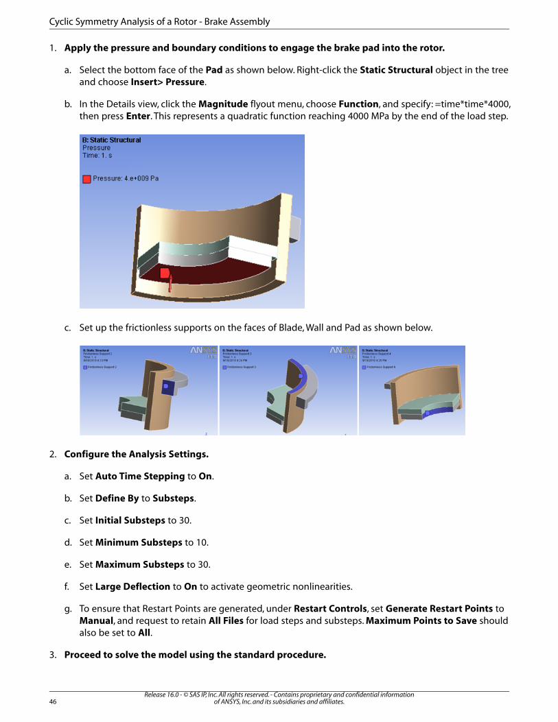
1. Apply the pressure and boundary conditions to engage the brake pad into the rotor.
a. Select the bottom face of the Pad as shown below. Right-click the Static Structural object in the treeand choose Insert> Pressure.
b. In the Details view, click the Magnitude flyout menu, choose Function, and specify: =time*time*4000,then press Enter. This represents a quadratic function reaching 4000 MPa by the end of the load step.
c. Set up the frictionless supports on the faces of Blade, Wall and Pad as shown below.
2. Configure the Analysis Settings.
a. Set Auto Time Stepping to On.
b. Set Define By to Substeps.
c. Set Initial Substeps to 30.
d. Set Minimum Substeps to 10.
e. Set Maximum Substeps to 30.
f. Set Large Deflection to On to activate geometric nonlinearities.
g. To ensure that Restart Points are generated, under Restart Controls, set Generate Restart Points toManual, and request to retain All Files for load steps and substeps. Maximum Points to Save shouldalso be set to All.
3. Proceed to solve the model using the standard procedure.
Release 16.0 - © SAS IP, Inc. All rights reserved. - Contains proprietary and confidential informationof ANSYS, Inc. and its subsidiaries and affiliates.46
Cyclic Symmetry Analysis of a Rotor - Brake Assembly
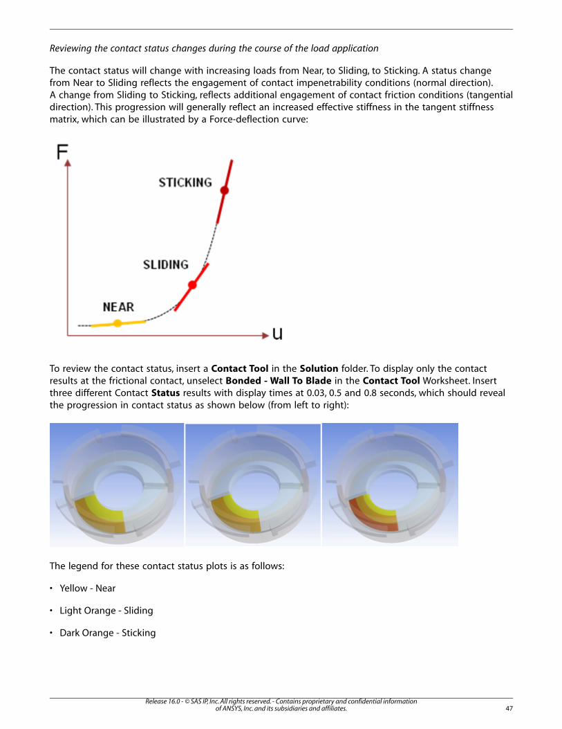
Reviewing the contact status changes during the course of the load application
The contact status will change with increasing loads from Near, to Sliding, to Sticking. A status changefrom Near to Sliding reflects the engagement of contact impenetrability conditions (normal direction).A change from Sliding to Sticking, reflects additional engagement of contact friction conditions (tangentialdirection). This progression will generally reflect an increased effective stiffness in the tangent stiffnessmatrix, which can be illustrated by a Force-deflection curve:
To review the contact status, insert a Contact Tool in the Solution folder. To display only the contactresults at the frictional contact, unselect Bonded - Wall To Blade in the Contact Tool Worksheet. Insertthree different Contact Status results with display times at 0.03, 0.5 and 0.8 seconds, which should revealthe progression in contact status as shown below (from left to right):
The legend for these contact status plots is as follows:
• Yellow - Near
• Light Orange - Sliding
• Dark Orange - Sticking
47Release 16.0 - © SAS IP, Inc. All rights reserved. - Contains proprietary and confidential information
of ANSYS, Inc. and its subsidiaries and affiliates.

Modal Analysis
There are three modal analyses to study the effect of contact status and stress stiffening on the freevibration response of the structure. Each of these will be based on a different restart point in the staticstructural analysis.
To see all available restart points, you can inspect the timeline graph displayed when the AnalysisSettings object of the Static Structural analysis is selected after solving. Restart points are denoted asblue triangle marks atop the graph:
To select the restart point of interest, go to the Pre-Stress (Static Structural) object under each ModalAnalysis. Make sure Pre-Stress Define By is set to Time and specify the time. The object will acknow-ledge the restart point in the Reported Loadstep, Reported Substep and Reported Time fields.
Configure the Modal analyses as follows:
• In Modal 1 set Pre-Stress Time to 0.033 seconds.
• In Modal 2 set Pre-Stress Time to 0.5 seconds.
• In Modal 3 set Pre-Stress Time to 0.8 seconds.
Because the boundary conditions (that is, the frictionless supports) are automatically imported fromthe static analysis, we can proceed directly to solve.
Solving and Reviewing Modal Results
We'll monitor the lowest frequencies of vibration which belong to Harmonic Indices 0 (symmetric) and2 (anti-symmetric).
1. Right-click on the Solution folder of each Modal analysis and choose Solve.
2. When the solutions complete, go to the Tabular Data window of each modal analysis. You can inspectthe listing of modes and their frequencies. Because our structure has a symmetry of N=4, there will bethree solutions, namely for Harmonic Indices 0, 1 and 2.
3. In the Tabular Data window of each modal analysis, select the two rows for Harmonic Index 0 - Mode 1and Harmonic Index 2 - Mode 1. Right-click and choose Create Mode Shape Results.
The image below shows this view for the first Modal analysis:
Release 16.0 - © SAS IP, Inc. All rights reserved. - Contains proprietary and confidential informationof ANSYS, Inc. and its subsidiaries and affiliates.48
Cyclic Symmetry Analysis of a Rotor - Brake Assembly

An interesting alternative to this view is to see the sorted frequency spectrum. You may review thisby setting the X-Axis to Frequency on any of the Total Deformation results in each modal analysis:
At this point, each modal analysis should have two results for Total Deformation to inspect the firstMode of Harmonic Indices 0 and 2.
Recall the meaning of Harmonic Index solutions and how they apply to the model. Harmonic Index0 represents the constant offset in the discrete Fourier Series representation of the model and cor-responds to equal values of every transformed quantity, for example, displacements in X, Y and Zdirections, in consecutive sectors. Thus deformations that are axially positive in one sector will havethe same axially positive value in the next. The following picture compiles, from left to right, themode shapes for the Near, Sliding and Sticking status at Harmonic Index 0:
Notice how increased engagement of the frictional contact in the assembly has the effect of producinghigher frequency vibrations. Also, the mode of vibration goes from being localized at the contactinterface when the contact is Near, but is forced to distribute throughout the wall of the rotor asthe contact sticks.
Note
You may need to specify Auto Scale on the Results toolbar so the mode shapes areplotted as shown.
49Release 16.0 - © SAS IP, Inc. All rights reserved. - Contains proprietary and confidential information
of ANSYS, Inc. and its subsidiaries and affiliates.

Harmonic Index 2 solutions correspond to N/2 for our sector (90 degrees or N = 4). This HarmonicIndex, sometimes called the asymmetric term in the Fourier Series, represents alternation of quant-ities in consecutive sectors. A positive axial displacement at a node in one sector becomes negativein the next, a radially outward displacement in one sector will become inward in the next, and soon. The following are the results for the first mode of this Harmonic Index:
The lowest mode shows nearly independent vibration of the rotor relative to the blade. On thehighest mode, sticking reduces this relative movement.
For a continued discussion on post-processing for Cyclic Symmetry and especially on features forpostprocessing degenerate Harmonic Indices (those between 0 and N/2), please see ReviewingResults for Cyclic Symmetry in a Modal Analysis in the Mechanical help.
End of tutorial.
Release 16.0 - © SAS IP, Inc. All rights reserved. - Contains proprietary and confidential informationof ANSYS, Inc. and its subsidiaries and affiliates.50
Cyclic Symmetry Analysis of a Rotor - Brake Assembly
Steady-State and Transient Thermal Analysis of a Circuit Board
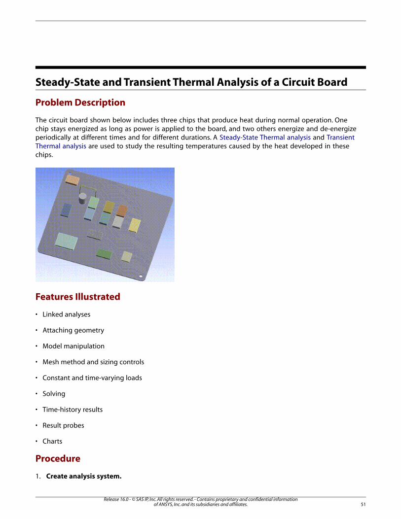
Problem Description
The circuit board shown below includes three chips that produce heat during normal operation. Onechip stays energized as long as power is applied to the board, and two others energize and de-energizeperiodically at different times and for different durations. A Steady-State Thermal analysis and TransientThermal analysis are used to study the resulting temperatures caused by the heat developed in thesechips.
Features Illustrated
• Linked analyses
• Attaching geometry
• Model manipulation
• Mesh method and sizing controls
• Constant and time-varying loads
• Solving
• Time-history results
• Result probes
• Charts
Procedure
1. Create analysis system.
51Release 16.0 - © SAS IP, Inc. All rights reserved. - Contains proprietary and confidential information
of ANSYS, Inc. and its subsidiaries and affiliates.

You need to establish a transient thermal analysis that is linked to a steady-state thermal analysis.
a. Start ANSYS Workbench.
b. From the Toolbox, drag a Steady-State Thermal system onto the Project Schematic.
c. From the Toolbox, drag a Transient Thermal system onto the Steady-State Thermal system suchthat cells 2, 3, 4, and 6 are highlighted in red.
d. Release the mouse button to define the linked analysis system.
2. Attach geometry.
a. In the Steady-State Thermal schematic, right-click the Geometry cell, and then choose Import Geo-metry.
b. Browse to open the file BoardWithChips.x_t. This file is available on the ANSYS Customer Portal;go to http://support.ansys.com/training.
3. Continue preparing the analysis in the Mechanical Application.
a. In the Steady-State Thermal schematic, right-click the Model cell, and then choose Edit. The Mechan-ical Application opens and displays the model.
b. For convenience , use the Rotate toolbar button to manipulate the model so it displays as shown below.
Release 16.0 - © SAS IP, Inc. All rights reserved. - Contains proprietary and confidential informationof ANSYS, Inc. and its subsidiaries and affiliates.52
Steady-State and Transient Thermal Analysis of a Circuit Board

Note
You can perform the same model manipulations by holding down the mouse wheelor middle button while dragging the mouse.
c. From the Menu bar , choose Units> Metric (m, kg, N, s, V, A) .
4. Set mesh controls and generate mesh.
Setting a specific mesh method control and mesh sizing controls will ensure a good quality mesh.
Mesh Method:
a. Right-click Mesh in the tree and choose Insert> Method.
b. Select all bodies by choosing Edit> Select All from the toolbar, then clicking the Apply button in theDetails view.
c. In the Details view, set Method to Hex Dominant, and Free Face Mesh Type to All Quad.
Mesh Body Sizing – Board Components:
a. Right-click Mesh in the tree and choose Insert> Sizing.
b. Select all bodies except the board by first enabling the Body selection toolbar button, then holdingthe Ctrl keyboard button and clicking on the 15 individual bodies. Click the Apply button in the Detailsview when you are done selecting the bodies.
c. Change Element Size from Default to 0.0009 m.
Mesh Body Sizing – Board:
a. Right-click Mesh in the tree and choose Insert> Sizing.
b. Select the board only and change Element Size from Default to 0.002 m.
Generate Mesh:
• Right-click Mesh in the tree and choose Generate Mesh.
53Release 16.0 - © SAS IP, Inc. All rights reserved. - Contains proprietary and confidential information
of ANSYS, Inc. and its subsidiaries and affiliates.
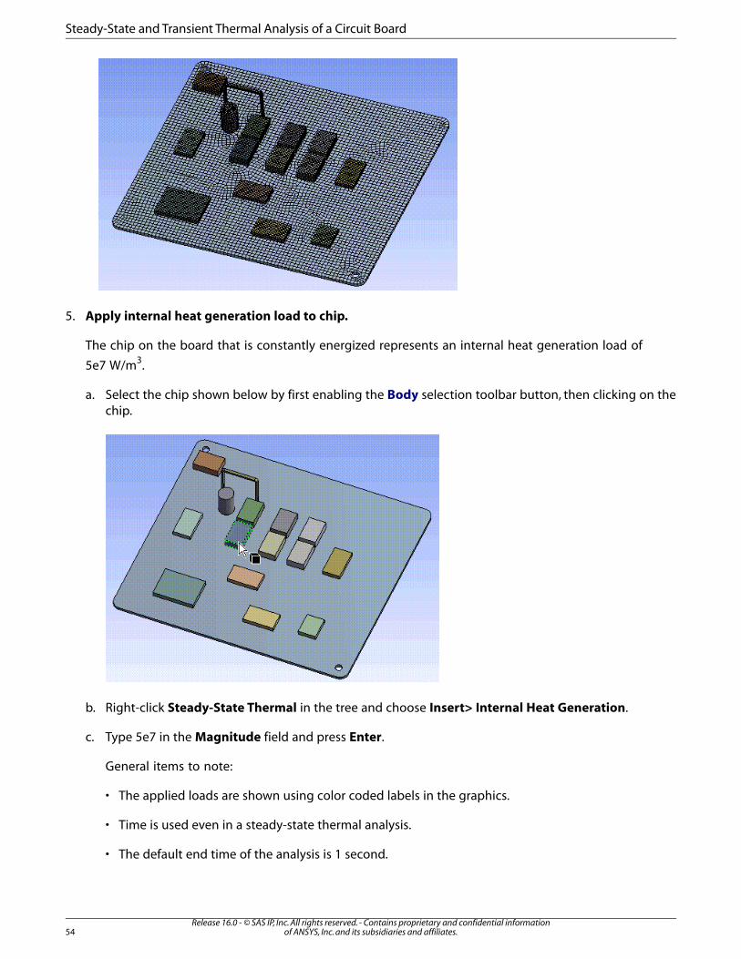
5. Apply internal heat generation load to chip.
The chip on the board that is constantly energized represents an internal heat generation load of
5e7 W/m3.
a. Select the chip shown below by first enabling the Body selection toolbar button, then clicking on thechip.
b. Right-click Steady-State Thermal in the tree and choose Insert> Internal Heat Generation.
c. Type 5e7 in the Magnitude field and press Enter.
General items to note:
• The applied loads are shown using color coded labels in the graphics.
• Time is used even in a steady-state thermal analysis.
• The default end time of the analysis is 1 second.
Release 16.0 - © SAS IP, Inc. All rights reserved. - Contains proprietary and confidential informationof ANSYS, Inc. and its subsidiaries and affiliates.54
Steady-State and Transient Thermal Analysis of a Circuit Board

• In a steady-state thermal analysis, the loads are ramped from zero. You can edit the table of load vs.time to modify the load behavior.
• You can also type in expressions that are functions of time for loads.
6. Apply a convection load to the entire circuit board.
The entire circuit board is subjected to a convection load representing Stagnant Air - SimplifiedCase.
a. Select all bodies by choosing Edit> Select All.
b. Choose Convection from the Environment toolbar.
c. Import temperature dependent convection coefficient and choose Stagnant Air - Simplified Case.
Note that the Ambient Temperature defaults to 22oC.
i. Click the flyout menu in the Film Coefficient field and choose Import Temperature Dependent(adjacent to the thermometer icon).
ii. Click the radio button for Stagnant Air - Simplified Case, then click OK.
7. Prepare for a temperature result.
The resulting temperature of the entire model will be reviewed.
• Right-click Solution in the tree under Steady-State Thermal and choose Insert> Thermal> Temperature.
8. Solve the steady-state thermal analysis.
• Choose Solve from the toolbar.
9. Review the temperature result.
• Highlight Temperature in the tree.
You have completed the steady-state thermal analysis, which is the first part of the overall objectivefor this tutorial. You will perform the transient thermal analysis in the remaining steps.
Items to note in preparation for the transient thermal analysis:
• If you highlight Initial Temperature under Transient Thermal in the tree, you will notice in the Detailsview, the read only displays of Initial Temperature and Initial Temperature Environment. In general,the initial temperature can be:
55Release 16.0 - © SAS IP, Inc. All rights reserved. - Contains proprietary and confidential information
of ANSYS, Inc. and its subsidiaries and affiliates.

– Uniform Temperature - where you specify a temperature for all bodies in the structure at time = 0,or
– Non-Uniform Temperature - (as in this example) where you import the temperature specification attime = 0 from a steady-state analysis.
• The initial temperature environment is from the steady-state thermal analysis that you just performed.By default the last set of results from the steady-state analysis will be used as the initial condition. Youcan specify a different set (different time point) if multiple result sets are available.
10. Specify a time duration for the transient analysis.
A time duration of the transient study will be 200 seconds.
• Under Transient Thermal, highlight the Analysis Settings object and enter 200 in either the Step EndTime field in the Details view or in the End Time column in the Tabular Data window. Also note andaccept the default initial, maximum, and minimum time step controls for this analysis.
11. Apply internal heat generation to simulate on/off switching on first chip.
A chip on the board is energized between 20 and 40 seconds and represents an internal heat gen-
eration load of 5e7 W/m3 during this period.
a. Select the chip shown below by first enabling the Body selection toolbar button, then clicking on thechip.
b. Right-click Transient Thermal in the tree and choose Insert> Internal Heat Generation.
c. Enter the following data in the Tabular Data window:
Release 16.0 - © SAS IP, Inc. All rights reserved. - Contains proprietary and confidential informationof ANSYS, Inc. and its subsidiaries and affiliates.56
Steady-State and Transient Thermal Analysis of a Circuit Board

• Time = 0; Internal Heat Generation = 0
Note
Enter each of the following sets of data in the row beneath the end time of 200 s.
• Time = 20; Internal Heat Generation = 0
• Time = 20.1; Internal Heat Generation = 5e7
• Time = 40; Internal Heat Generation = 5e7
• Time = 40.1; Internal Heat Generation = 0
The Graph window reflects the data that you entered.
General items to note:
• Loads can be specified as one of three types:
– Constant – remains constant throughout the time history of the transient.
– Tabular (Time) – (as in this example) define a table of load vs. time.
– Function – enter a function such as “=10*sin(time)” to define a variation of load with respect totime. The function definition requires you to start with a ‘=‘ as the first character.
12. Apply internal heat generation to simulate on/off switching on second chip.
Another chip on the board is energized between 60 and 70 seconds and represents an internal heat
generation load of 1e8 W/m3 during this period.
a. Select the chip shown below by first enabling the Body selection toolbar button, then clicking on thechip.
57Release 16.0 - © SAS IP, Inc. All rights reserved. - Contains proprietary and confidential information
of ANSYS, Inc. and its subsidiaries and affiliates.

b. Right-click Transient Thermal in the tree and choose Insert> Internal Heat Generation.
c. Enter the following data in the Tabular Data window:
• Time = 0; Internal Heat Generation = 0
Note
Enter each of the following sets of data in the row beneath the end time of 200 s.
• Time = 60; Internal Heat Generation = 0
• Time = 60.1; Internal Heat Generation = 1e8
• Time = 70; Internal Heat Generation = 1e8
• Time = 70.1; Internal Heat Generation = 0
The Graph window reflects the data that you entered.
13. Prepare for a temperature result.
The resulting temperature of the entire model will be reviewed.
• Right-click Solution in the tree under Transient Thermal and choose Insert> Thermal> Temperature.
14. Solve the transient thermal analysis.
Release 16.0 - © SAS IP, Inc. All rights reserved. - Contains proprietary and confidential informationof ANSYS, Inc. and its subsidiaries and affiliates.58
Steady-State and Transient Thermal Analysis of a Circuit Board

• Click the right mouse button again on Solution and choose Solve. The solution is complete when greenchecks are displayed next to all of the objects. You can ignore the Warning message and click the Graphtab.
15. Review the time history of the temperature result for the entire model.
• Highlight the Temperature object. The time history of the temperature result for the entire model isevaluated and displayed.
– The Tabular Data window shows the min/max values of temperature at a time point.
– By moving the mouse, you can move the bar along the Graph as shown, to any time, click the rightmouse button and Retrieve this Result to review the results at a particular time.
– You can also animate the solution.
16. Review the time history of the temperature result for each of the chips.
Temperature probes are used to obtain temperatures at specific locations on the model.
a. Right-click Solution and choose Insert> Probe> Temperature.
b. Select the chip to which internal heat generation was applied in the steady state analysis and click theApply button in the Details view.
c. Follow the same procedure to insert two more probes for the two chips with internal heat generationsin the transient thermal analysis.
d. Right-click Solution or Temperature Probe and choose Evaluate All Results.
17. Plot probe results on a chart.
a. Select the three temperature probes in the tree and select the New Chart and Table button from thetoolbar.
A Chart object is added to the tree.
59Release 16.0 - © SAS IP, Inc. All rights reserved. - Contains proprietary and confidential information
of ANSYS, Inc. and its subsidiaries and affiliates.
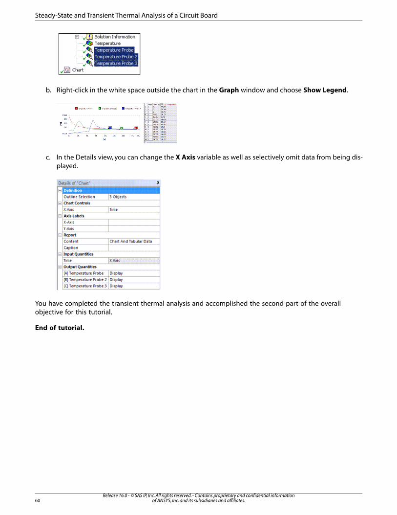
b. Right-click in the white space outside the chart in the Graph window and choose Show Legend.
c. In the Details view, you can change the X Axis variable as well as selectively omit data from being dis-played.
You have completed the transient thermal analysis and accomplished the second part of the overallobjective for this tutorial.
End of tutorial.
Release 16.0 - © SAS IP, Inc. All rights reserved. - Contains proprietary and confidential informationof ANSYS, Inc. and its subsidiaries and affiliates.60
Steady-State and Transient Thermal Analysis of a Circuit Board

Delamination Analysis using Contact Based Debonding Capability
Problem Description
This tutorial demonstrates the use of Contact Debonding feature available in Mechanical by examiningthe displacement of two 2D parts on a double cantilever beam. This same problem is demonstrated inVM255. The following example is provided to demonstrate the steps to setup and analyze the samemodel using Mechanical.
As illustrated below, a two dimensional beam has a length of 100mm and an initial crack of length of30mm at the free end that is subjected to a maximum vertical displacement (Umax) at the top and
bottom of the free end nodes. Two vertical displacements, one positive and one negative, are appliedto determine the vertical reaction at the end point. The point of fracture is at the vertex of the crackand the interface edges.
This tutorial also examines how to prepare the necessary materials that work in cooperation with theContact Debonding feature.
Features Demonstrated
• Engineering Data/Materials
• Static Structural Analysis
61Release 16.0 - © SAS IP, Inc. All rights reserved. - Contains proprietary and confidential information
of ANSYS, Inc. and its subsidiaries and affiliates.

• Contact Regions
• Contact Debonding
Procedure
1. Create static structural analysis.
a. Open ANSYS Workbench.
b. On the Workbench Project page, drag a Static Structural system from the Toolbox to the ProjectSchematic. The Project Schematic should appear as follows. The properties window does not displayunless you have made the required selection; right-click a cell and select Properties.
2. Define materials.
a. In the Static Structural schematic, right-click the Engineering Data cell and choose Edit. The Engin-eering Data tab opens and displays Structural Steel as the default material.
b. Click the box below the field labeled "Click here to add new material" and enter the name "InterfaceBody Material".
c. Expand the Linear Elastic option in the Toolbox and right-click Orthotropic Elasticity. Select IncludeProperty. The required properties for the material are highlighted in yellow.
Release 16.0 - © SAS IP, Inc. All rights reserved. - Contains proprietary and confidential informationof ANSYS, Inc. and its subsidiaries and affiliates.62
Delamination Analysis using Contact Based Debonding Capability

d. Define the new material by entering the following property values and units of measure into the cor-responding fields.
UnitValueProperty
MPa1.353E+05Young’s Modulus X Direction
MPa9000Young’s Modulus Y Direction
MPa9000Young’s Modulus Z Direction
NA0.24Poisson’s Ratio XY
NA0.46Poisson’s Ratio YZ
NA0.24Poisson’s Ratio XZ
MPa5200Shear Modulus XY
MPa0.0001Shear Modulus YZ
MPa0.0001Shear Modulus XZ
Once complete, the properties for the material should appear as follows.
e. Now you need to create a new Material that specifies the formulation used to introduce the fracturemechanism. For this tutorial, the Cohesive Zone Material (CZM) method is used. Click the field labeled"Click here to add new material" and enter the name “CZM Crack Material”.
63Release 16.0 - © SAS IP, Inc. All rights reserved. - Contains proprietary and confidential information
of ANSYS, Inc. and its subsidiaries and affiliates.

f. Expand the Cohesive Zone option in the Toolbox and right-click Fracture-Energies based Debonding.Select Include Property. The required properties for the material are highlighted in yellow.
g. Define the new material by entering the following property values and units of measure into the cor-responding fields.
UnitValueProperty
NANoTangential Slip Under Normal Compression
Pa1.7E+06Maximum Normal Contact Stress
Jm^-2
280Critical Fracture Energy for Normal Separation
Pa1E-30Maximum Equivalent Tangential ContactStress
Jm^-2
1E-30Critical Fracture Energy for Tangential Slip
s1e-8Artificial Damping Coefficient
The properties for the material should appear as follows.
Release 16.0 - © SAS IP, Inc. All rights reserved. - Contains proprietary and confidential informationof ANSYS, Inc. and its subsidiaries and affiliates.64
Delamination Analysis using Contact Based Debonding Capability
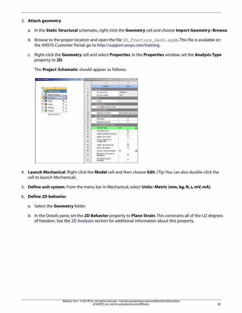
3. Attach geometry.
a. In the Static Structural schematic, right-click the Geometry cell and choose Import Geometry>Browse.
b. Browse to the proper location and open the file 2D_Fracture_Geom.agdb. This file is available onthe ANSYS Customer Portal; go to http://support.ansys.com/training.
c. Right-click the Geometry cell and select Properties. In the Properties window, set the Analysis Typeproperty to 2D.
The Project Schematic should appear as follows:
4. Launch Mechanical. Right-click the Model cell and then choose Edit. (Tip: You can also double-click thecell to launch Mechanical).
5. Define unit system. From the menu bar in Mechanical, select Units>Metric (mm, kg, N, s, mV, mA).
6. Define 2D behavior.
a. Select the Geometry folder.
b. In the Details pane, set the 2D Behavior property to Plane Strain. This constrains all of the UZ degreesof freedom. See the 2D Analyses section for additional information about this property.
65Release 16.0 - © SAS IP, Inc. All rights reserved. - Contains proprietary and confidential information
of ANSYS, Inc. and its subsidiaries and affiliates.
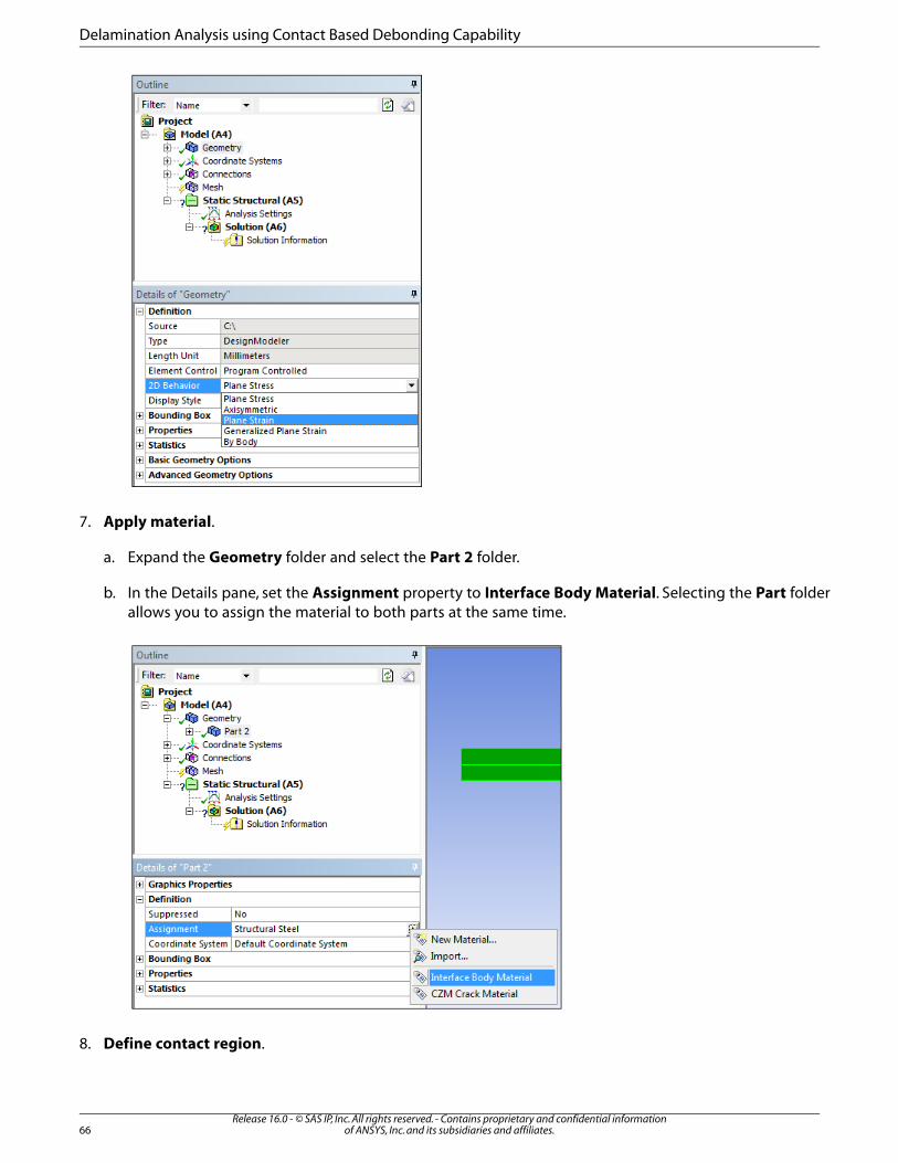
7. Apply material.
a. Expand the Geometry folder and select the Part 2 folder.
b. In the Details pane, set the Assignment property to Interface Body Material. Selecting the Part folderallows you to assign the material to both parts at the same time.
8. Define contact region.
Release 16.0 - © SAS IP, Inc. All rights reserved. - Contains proprietary and confidential informationof ANSYS, Inc. and its subsidiaries and affiliates.66
Delamination Analysis using Contact Based Debonding Capability
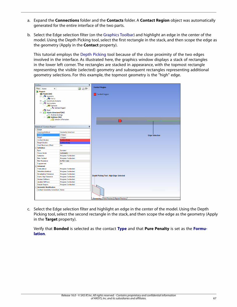
a. Expand the Connections folder and the Contacts folder. A Contact Region object was automaticallygenerated for the entire interface of the two parts.
b. Select the Edge selection filter (on the Graphics Toolbar) and highlight an edge in the center of themodel. Using the Depth Picking tool, select the first rectangle in the stack, and then scope the edge asthe geometry (Apply in the Contact property).
This tutorial employs the Depth Picking tool because of the close proximity of the two edgesinvolved in the interface. As illustrated here, the graphics window displays a stack of rectanglesin the lower left corner. The rectangles are stacked in appearance, with the topmost rectanglerepresenting the visible (selected) geometry and subsequent rectangles representing additionalgeometry selections. For this example, the topmost geometry is the "high" edge.
c. Select the Edge selection filter and highlight an edge in the center of the model. Using the DepthPicking tool, select the second rectangle in the stack, and then scope the edge as the geometry (Applyin the Target property).
Verify that Bonded is selected as the contact Type and that Pure Penalty is set as the Formu-lation.
67Release 16.0 - © SAS IP, Inc. All rights reserved. - Contains proprietary and confidential information
of ANSYS, Inc. and its subsidiaries and affiliates.
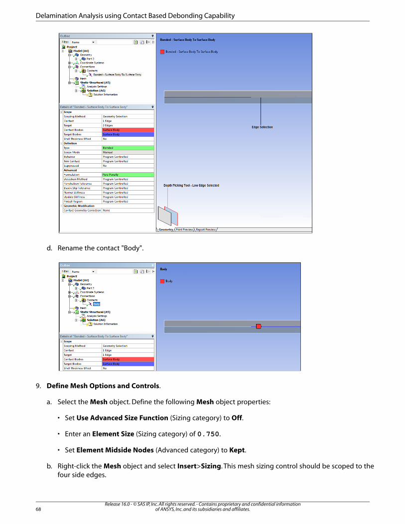
d. Rename the contact "Body".
9. Define Mesh Options and Controls.
a. Select the Mesh object. Define the following Mesh object properties:
• Set Use Advanced Size Function (Sizing category) to Off.
• Enter an Element Size (Sizing category) of 0.750.
• Set Element Midside Nodes (Advanced category) to Kept.
b. Right-click the Mesh object and select Insert>Sizing. This mesh sizing control should be scoped to thefour side edges.
Release 16.0 - © SAS IP, Inc. All rights reserved. - Contains proprietary and confidential informationof ANSYS, Inc. and its subsidiaries and affiliates.68
Delamination Analysis using Contact Based Debonding Capability

c. In the Details view, enter 0.75 mm as the Element Size.
d. Select the Edge selection filter (on the Graphics Toolbar) and highlight an edge in the center of themodel. Use the Depth Picking tool and, holding the Ctrl key, select both rectangles in the lower leftcorner of the graphics window. Continue to hold the Ctrl key, and select an edge of the crack. Again,use the Depth Picking tool and select both rectangles in the lower left corner of the graphics window.Still holding the Ctrl key, select the top and bottom edges on the model.
e. Right-click the Mesh object and select Insert>Sizing. This mesh sizing control should be scoped to six(top and bottom and the four interface edges) edges.
f. In the Details view, enter 0.5 mm as the Element Size.
g. Right-click the Mesh object and select Generate Mesh.
10. Specify Contact Debonding object.
a. Insert a Fracture folder into the tree by highlighting the Model object and then selecting the Fracturebutton on the Model Context Toolbar.
69Release 16.0 - © SAS IP, Inc. All rights reserved. - Contains proprietary and confidential information
of ANSYS, Inc. and its subsidiaries and affiliates.

b. Right-click and select Insert>Contact Debonding. You could also select the Contact Debondingbutton on the Fracture Context Toolbar.
c. In the Details pane, set the Material property to CZM Crack Material.
Release 16.0 - © SAS IP, Inc. All rights reserved. - Contains proprietary and confidential informationof ANSYS, Inc. and its subsidiaries and affiliates.70
Delamination Analysis using Contact Based Debonding Capability

d. In the Details pane, set the Contact Region property to Body.
The Contact Debonding object is complete.
71Release 16.0 - © SAS IP, Inc. All rights reserved. - Contains proprietary and confidential information
of ANSYS, Inc. and its subsidiaries and affiliates.

11. Configure the Analysis Settings.
a. Select the Analysis Settings object.
b. Set the Auto Time Setting property to On and then enter 100 for the Initial Substeps, MinimumSubsteps, and Maximum Substeps properties.
12. Apply boundary conditions.
a. Select the Edge selection filter and select the two edges on the side of the model that is opposite ofthe crack. Select one edge, press the Ctrl key, and then select the next edge.
Release 16.0 - © SAS IP, Inc. All rights reserved. - Contains proprietary and confidential informationof ANSYS, Inc. and its subsidiaries and affiliates.72
Delamination Analysis using Contact Based Debonding Capability

b. Highlight the Static Structural object, select the Supports menu on the Environment Context Toolbar,and then select Fixed Support.
c. Highlight the Static Structural object. With the Vertex selection filter active, select the vertex illustratedbelow, select the Supports menu and then select Displacement.
In the Details pane, enter 10 (mm in the positive Y direction) as the loading value for the YComponent property.
d. Create another Displacement. With the Vertex selection filter active, select the bottom vertex, andthen select Supports>Displacement. Enter -10 (mm in the negative Y direction) as the loading valuefor the Y Component property.
73Release 16.0 - © SAS IP, Inc. All rights reserved. - Contains proprietary and confidential information
of ANSYS, Inc. and its subsidiaries and affiliates.

13. Specify result objects and solve.
a. Highlight the Solution object, select the Deformation menu on the Solution Context Toolbar, andthen select Directional Deformation.
b. Under the Definition category in the Details view, set the Orientation property to Y Axis.
c. Highlight the Solution object, select the Probe menu on the Solution Context Toolbar, and then selectForce Reaction.
d. Select Displacement for the Boundary Condition property of the probe.
e. Click the Solve button.
14. Review the results. Highlight the Directional Deformation and Force Reaction objects. Results appearas follows:
Release 16.0 - © SAS IP, Inc. All rights reserved. - Contains proprietary and confidential informationof ANSYS, Inc. and its subsidiaries and affiliates.74
Delamination Analysis using Contact Based Debonding Capability

You may wish to validate results against those outlined in the verification test case (VM255). This ismost easily accomplished by creating User Defined Results using the Worksheet.
End of tutorial.
75Release 16.0 - © SAS IP, Inc. All rights reserved. - Contains proprietary and confidential information
of ANSYS, Inc. and its subsidiaries and affiliates.

Release 16.0 - © SAS IP, Inc. All rights reserved. - Contains proprietary and confidential informationof ANSYS, Inc. and its subsidiaries and affiliates.76

Interface Delamination Analysis of Double Cantilever Beam
Problem Description
This tutorial demonstrates the use of Interface Delamination feature available in Mechanical by examiningthe displacement of two 2D parts on a double cantilever beam. This same problem is demonstrated inVM248. The following example is provided to demonstrate the steps to setup and analyze the samemodel using Mechanical.
As illustrated below, a two dimensional beam has a length of 100mm and an initial crack of length of30mm at the free end that is subjected to a maximum vertical displacement (Umax) at the top and
bottom of the free end nodes. Two vertical displacements, one positive and one negative, are appliedto determine the vertical reaction at the end point. The point of fracture is at the vertex of the crackand the interface edges.
This image illustrates the dimension of the model.
This tutorial also examines how to prepare the necessary materials and mesh controls that work in co-operation with the Interface Delamination feature.
Features Demonstrated
• Engineering Data/Materials
77Release 16.0 - © SAS IP, Inc. All rights reserved. - Contains proprietary and confidential information
of ANSYS, Inc. and its subsidiaries and affiliates.

• Static Structural Analysis
• Match Control
• Interface Delamination
Procedure
1. Create static structural analysis.
a. Open ANSYS Workbench.
b. On the Workbench Project page, drag a Static Structural system from the Toolbox to the ProjectSchematic. The Project Schematic should appear as follows. The properties window does not displayunless you have made the required selection; right-click a cell and select Properties.
Note
The Interface Delamination feature is only available for Static Structural and TransientStructural analyses.
2. Assign materials.
This analysis requires the creation of the proper materials using the Engineering Data feature ofWorkbench. We will define a new Orthotropic Elastic material for the model as well as a CohesiveZone Bilinear material for the Interface Delamination feature.
a. In the Static Structural schematic, right-click the Engineering Data cell and choose Edit. The Engin-eering Data tab opens and displays Structural Steel as the default material.
b. Click the box labeled "Click here to add new material" and enter the name "Interface Body Material".
c. Expand the Linear Elastic option in the Toolbox and right-click Orthotropic Elasticity. Select IncludeProperty. The required properties for the material are highlighted in yellow.
Release 16.0 - © SAS IP, Inc. All rights reserved. - Contains proprietary and confidential informationof ANSYS, Inc. and its subsidiaries and affiliates.78
Interface Delamination Analysis of Double Cantilever Beam

d. Define the new material by entering the following property values and units of measure into the cor-responding fields.
UnitValueProperty
MPa1.353E+05Young’s Modulus X Direction
MPa9000Young’s Modulus Y Direction
MPa9000Young’s Modulus Z Direction
na0.24Poisson’s Ratio XY
na0.46Poisson’s Ratio YZ
na0.24Poisson’s Ratio XZ
MPa5200Shear Modulus XY
MPa0.0001Shear Modulus YZ
MPa0.0001Shear Modulus XZ
The properties for the material should appear as follows:
e. Click the box labeled "Click here to add new material" and enter the name “CZM Material”. This mater-ial will specify the formulation used to introduce the fracture mechanism (Cohesive Zone Materialmethod).
79Release 16.0 - © SAS IP, Inc. All rights reserved. - Contains proprietary and confidential information
of ANSYS, Inc. and its subsidiaries and affiliates.
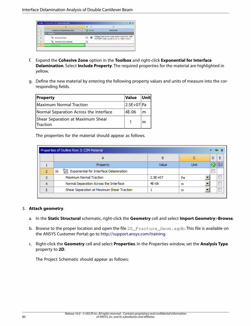
f. Expand the Cohesive Zone option in the Toolbox and right-click Exponential for InterfaceDelamination. Select Include Property. The required properties for the material are highlighted inyellow.
g. Define the new material by entering the following property values and units of measure into the cor-responding fields.
UnitValueProperty
Pa2.5E+07Maximum Normal Traction
m4E-06Normal Separation Across the Interface
m1Shear Separation at Maximum ShearTraction
The properties for the material should appear as follows.
3. Attach geometry.
a. In the Static Structural schematic, right-click the Geometry cell and select Import Geometry>Browse.
b. Browse to the proper location and open the file 2D_Fracture_Geom.agdb. This file is available onthe ANSYS Customer Portal; go to http://support.ansys.com/training.
c. Right-click the Geometry cell and select Properties. In the Properties window, set the Analysis Typeproperty to 2D.
The Project Schematic should appear as follows:
Release 16.0 - © SAS IP, Inc. All rights reserved. - Contains proprietary and confidential informationof ANSYS, Inc. and its subsidiaries and affiliates.80
Interface Delamination Analysis of Double Cantilever Beam

4. Launch Mechanical. Right-click the Model cell and then choose Edit. (Tip: You can also double-click thecell to launch Mechanical).
5. Define unit system. From the menu bar in Mechanical, select Units>Metric (mm, kg, N, s, mV, mA).
6. Define 2D behavior.
a. Highlight the Geometry folder.
b. In the Details pane, specify the 2D Behavior property as Plane Strain. This constrains all of the UZdegrees of freedom. See the 2D Analyses section for additional information about this property.
81Release 16.0 - © SAS IP, Inc. All rights reserved. - Contains proprietary and confidential information
of ANSYS, Inc. and its subsidiaries and affiliates.
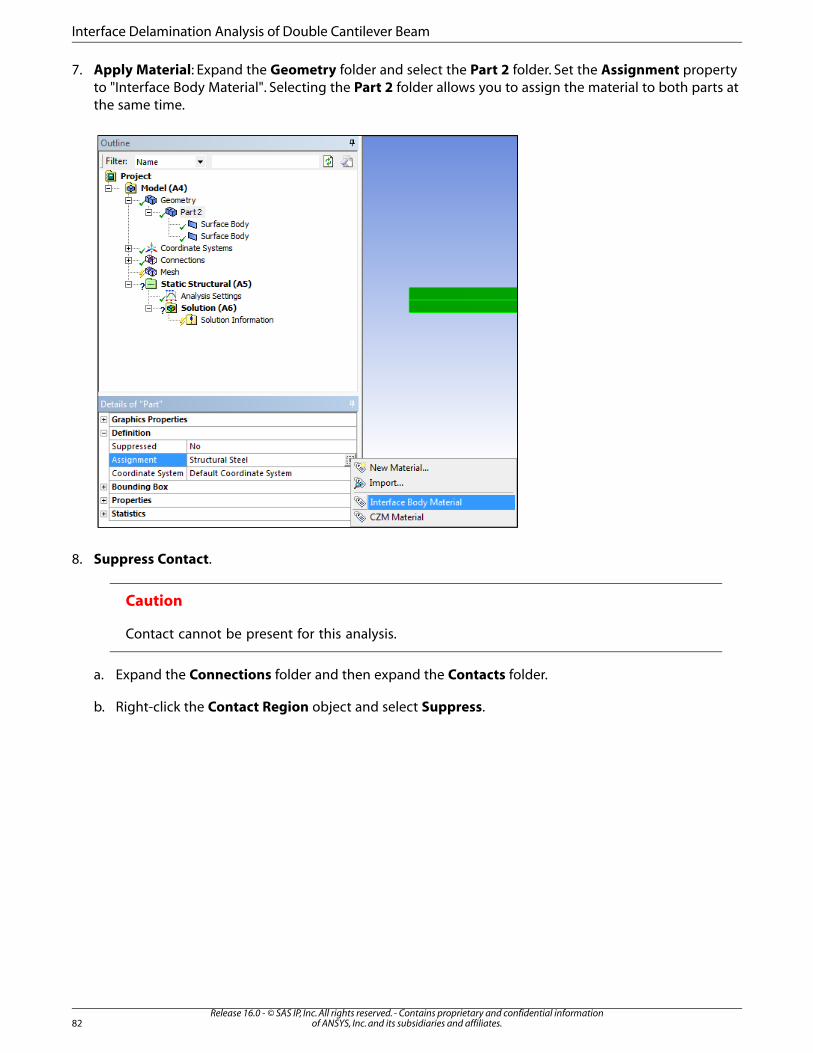
7. Apply Material: Expand the Geometry folder and select the Part 2 folder. Set the Assignment propertyto "Interface Body Material". Selecting the Part 2 folder allows you to assign the material to both parts atthe same time.
8. Suppress Contact.
Caution
Contact cannot be present for this analysis.
a. Expand the Connections folder and then expand the Contacts folder.
b. Right-click the Contact Region object and select Suppress.
Release 16.0 - © SAS IP, Inc. All rights reserved. - Contains proprietary and confidential informationof ANSYS, Inc. and its subsidiaries and affiliates.82
Interface Delamination Analysis of Double Cantilever Beam
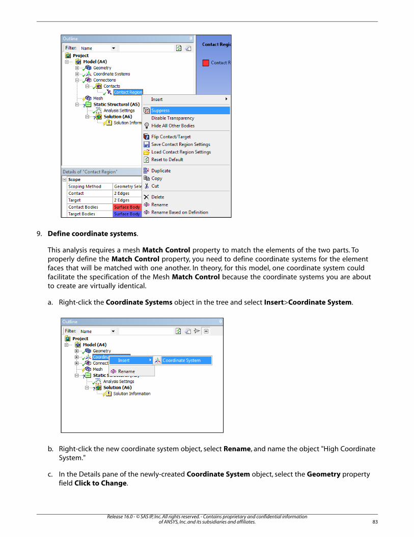
9. Define coordinate systems.
This analysis requires a mesh Match Control property to match the elements of the two parts. Toproperly define the Match Control property, you need to define coordinate systems for the elementfaces that will be matched with one another. In theory, for this model, one coordinate system couldfacilitate the specification of the Mesh Match Control because the coordinate systems you are aboutto create are virtually identical.
a. Right-click the Coordinate Systems object in the tree and select Insert>Coordinate System.
b. Right-click the new coordinate system object, select Rename, and name the object "High CoordinateSystem."
c. In the Details pane of the newly-created Coordinate System object, select the Geometry propertyfield Click to Change.
83Release 16.0 - © SAS IP, Inc. All rights reserved. - Contains proprietary and confidential information
of ANSYS, Inc. and its subsidiaries and affiliates.
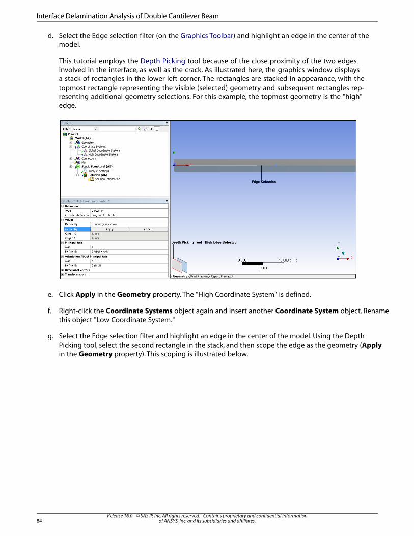
d. Select the Edge selection filter (on the Graphics Toolbar) and highlight an edge in the center of themodel.
This tutorial employs the Depth Picking tool because of the close proximity of the two edgesinvolved in the interface, as well as the crack. As illustrated here, the graphics window displaysa stack of rectangles in the lower left corner. The rectangles are stacked in appearance, with thetopmost rectangle representing the visible (selected) geometry and subsequent rectangles rep-resenting additional geometry selections. For this example, the topmost geometry is the "high"edge.
e. Click Apply in the Geometry property. The "High Coordinate System" is defined.
f. Right-click the Coordinate Systems object again and insert another Coordinate System object. Renamethis object "Low Coordinate System."
g. Select the Edge selection filter and highlight an edge in the center of the model. Using the DepthPicking tool, select the second rectangle in the stack, and then scope the edge as the geometry (Applyin the Geometry property). This scoping is illustrated below.
Release 16.0 - © SAS IP, Inc. All rights reserved. - Contains proprietary and confidential informationof ANSYS, Inc. and its subsidiaries and affiliates.84
Interface Delamination Analysis of Double Cantilever Beam
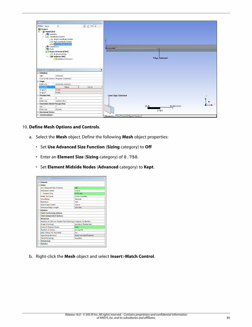
10. Define Mesh Options and Controls.
a. Select the Mesh object. Define the following Mesh object properties:
• Set Use Advanced Size Function (Sizing category) to Off
• Enter an Element Size (Sizing category) of 0.750.
• Set Element Midside Nodes (Advanced category) to Kept.
b. Right-click the Mesh object and select Insert>Match Control.
85Release 16.0 - © SAS IP, Inc. All rights reserved. - Contains proprietary and confidential information
of ANSYS, Inc. and its subsidiaries and affiliates.
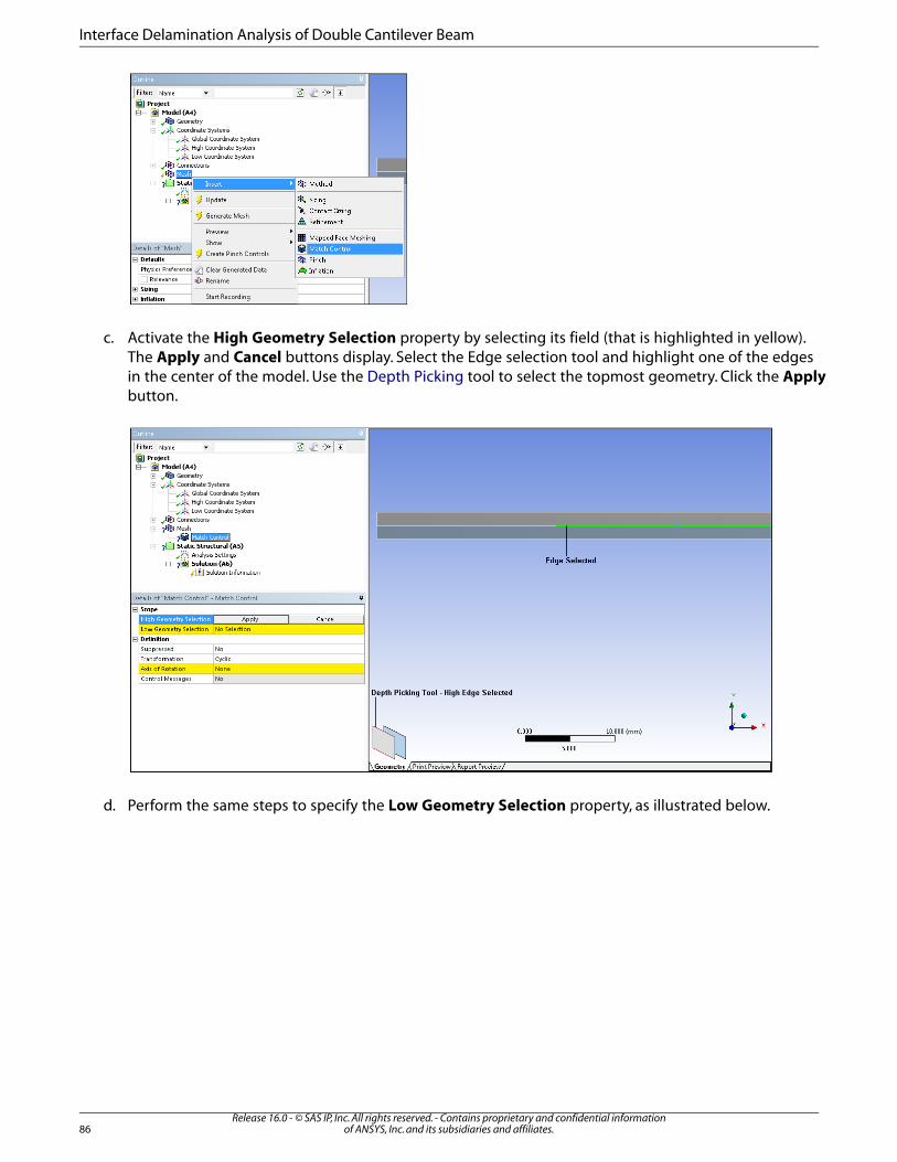
c. Activate the High Geometry Selection property by selecting its field (that is highlighted in yellow).The Apply and Cancel buttons display. Select the Edge selection tool and highlight one of the edgesin the center of the model. Use the Depth Picking tool to select the topmost geometry. Click the Applybutton.
d. Perform the same steps to specify the Low Geometry Selection property, as illustrated below.
Release 16.0 - © SAS IP, Inc. All rights reserved. - Contains proprietary and confidential informationof ANSYS, Inc. and its subsidiaries and affiliates.86
Interface Delamination Analysis of Double Cantilever Beam

e. Change the Transformation property from Cyclic to Arbitrary and specify the High Coordinate Systemand Low Coordinate System properties using the coordinate systems created in the previous step ofthe tutorial. The object should appear as illustrated below.
f. Select the Edge selection filter (on the Graphics Toolbar) and, holding the Ctrl key, select the four sideedges.
87Release 16.0 - © SAS IP, Inc. All rights reserved. - Contains proprietary and confidential information
of ANSYS, Inc. and its subsidiaries and affiliates.

g. Right-click the Mesh object and select Insert>Sizing. This mesh sizing control should be scoped to thefour side edges.
h. In the Details view, enter 0.75 mm as the Element Size.
i. Select the Edge selection filter (on the Graphics Toolbar) and highlight an edge in the center of themodel. Use the Depth Picking tool and, holding the Ctrl key, select both rectangles in the lower leftcorner of the graphics window. Continue to hold the Ctrl key, and select an edge of the crack. Again,use the Depth Picking tool and select both rectangles in the lower left corner of the graphics window.Still holding the Ctrl key, select the top and bottom edges on the model.
j. Right-click the Mesh object and select Insert>Sizing. This mesh sizing control should be scoped to six(top and bottom and the four interface edges) edges.
k. In the Details view, enter 0.5 mm as the Element Size.
l. Right-click the Mesh object and select Generate Mesh.
Release 16.0 - © SAS IP, Inc. All rights reserved. - Contains proprietary and confidential informationof ANSYS, Inc. and its subsidiaries and affiliates.88
Interface Delamination Analysis of Double Cantilever Beam

11. Define Interface Delamination object.
a. Insert a Fracture folder into the tree by highlighting the Model object and selecting the Fracturebutton on the Model Context Toolbar.
b. Select the Interface Delamination button on the Fracture Context Toolbar.
c. In the Details pane, set the Method property to CZM.
89Release 16.0 - © SAS IP, Inc. All rights reserved. - Contains proprietary and confidential information
of ANSYS, Inc. and its subsidiaries and affiliates.

d. Set the Material property to CZM Material.
e. Select the Match Control that was created earlier in the tutorial for the Match Control property.
Release 16.0 - © SAS IP, Inc. All rights reserved. - Contains proprietary and confidential informationof ANSYS, Inc. and its subsidiaries and affiliates.90
Interface Delamination Analysis of Double Cantilever Beam
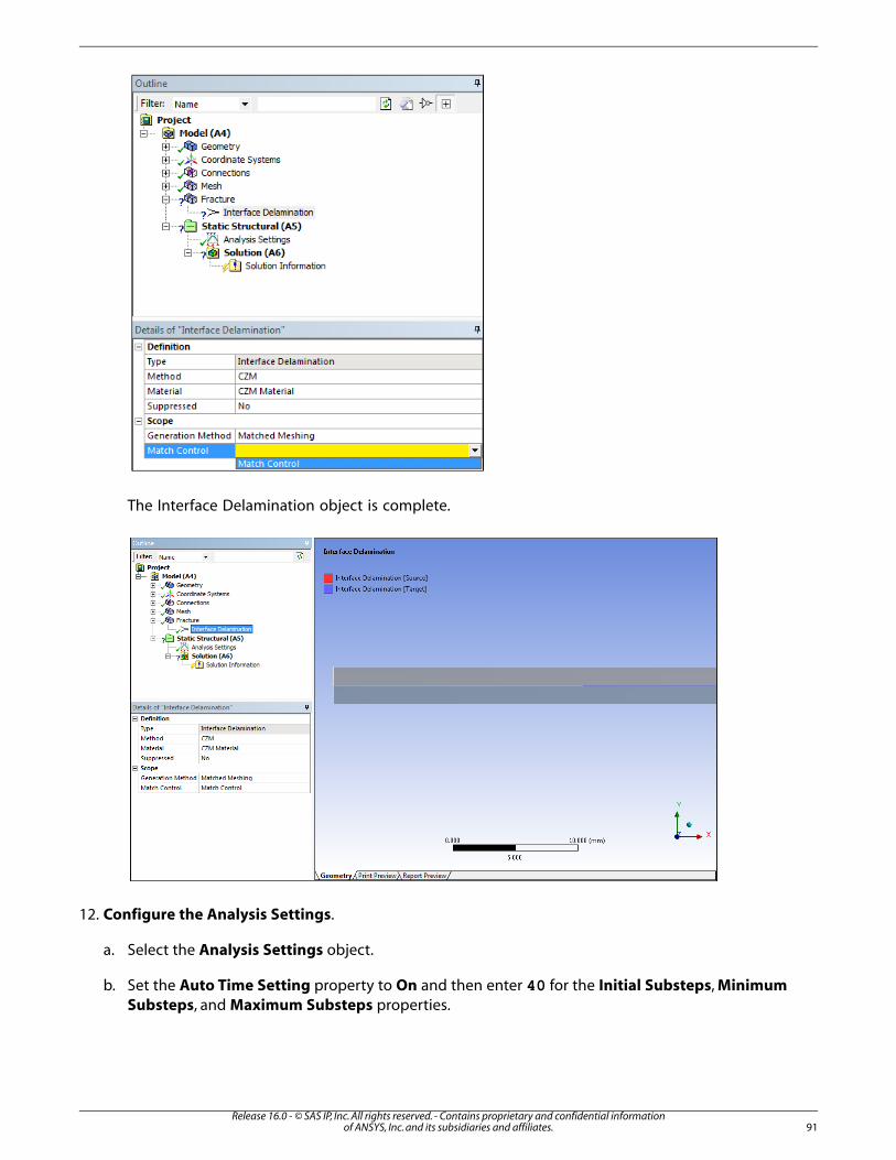
The Interface Delamination object is complete.
12. Configure the Analysis Settings.
a. Select the Analysis Settings object.
b. Set the Auto Time Setting property to On and then enter 40 for the Initial Substeps, MinimumSubsteps, and Maximum Substeps properties.
91Release 16.0 - © SAS IP, Inc. All rights reserved. - Contains proprietary and confidential information
of ANSYS, Inc. and its subsidiaries and affiliates.
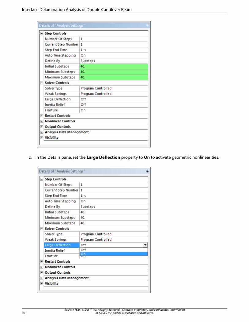
c. In the Details pane, set the Large Deflection property to On to activate geometric nonlinearities.
Release 16.0 - © SAS IP, Inc. All rights reserved. - Contains proprietary and confidential informationof ANSYS, Inc. and its subsidiaries and affiliates.92
Interface Delamination Analysis of Double Cantilever Beam

13. Define boundary conditions.
a. Select the Edge selection filter and select the two edges on the side of the model that is opposite ofthe crack. Select one edge, press the Ctrl key, and then select the next edge.
b. Highlight the Static Structural object, select the Supports menu on the Environment Context Toolbar,and then select Fixed Support.
c. Highlight the Static Structural object. With the Vertex selection filter active, select the vertex illustratedbelow, select the Supports menu, and then select Displacement.
d. Highlight the Displacement object in the tree and enter 10 (mm in the positive Y direction) as theloading value for the Y Component property.
93Release 16.0 - © SAS IP, Inc. All rights reserved. - Contains proprietary and confidential information
of ANSYS, Inc. and its subsidiaries and affiliates.
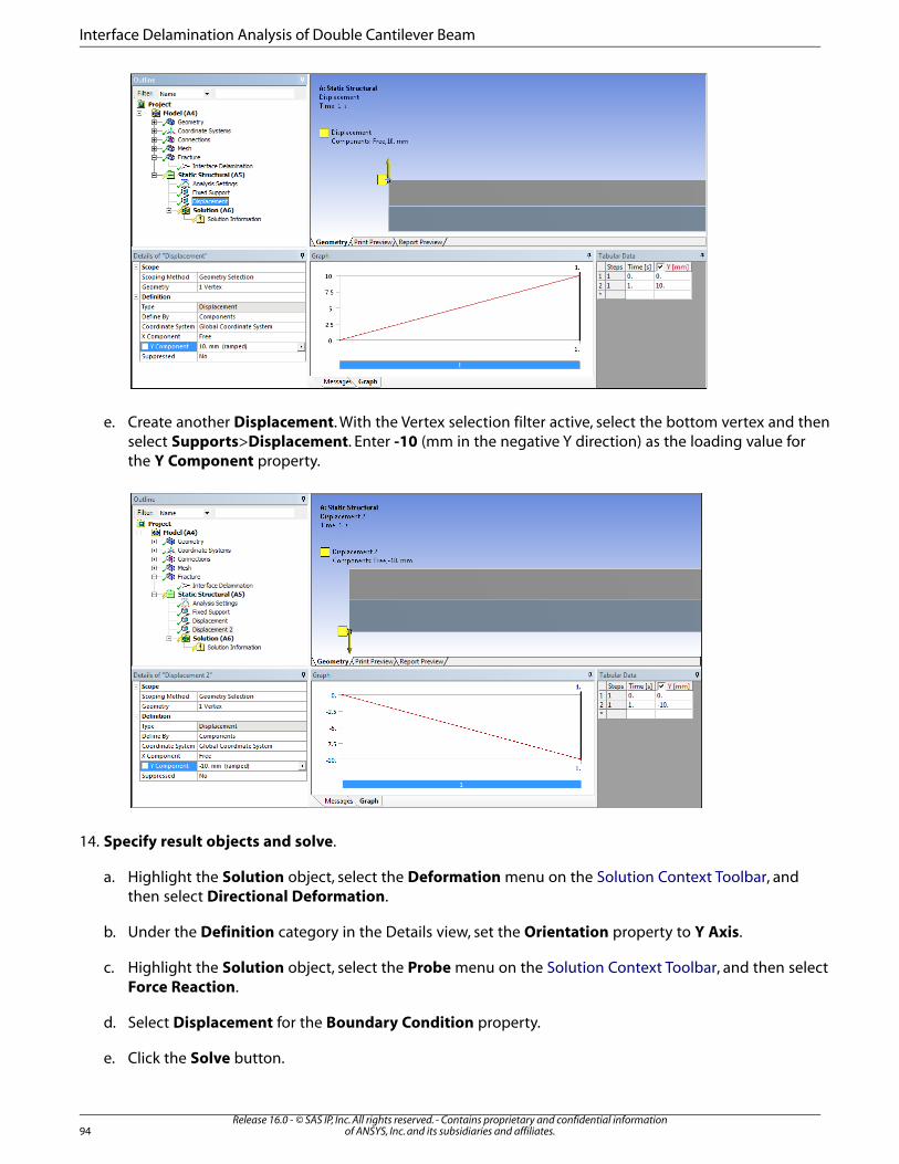
e. Create another Displacement. With the Vertex selection filter active, select the bottom vertex and thenselect Supports>Displacement. Enter -10 (mm in the negative Y direction) as the loading value forthe Y Component property.
14. Specify result objects and solve.
a. Highlight the Solution object, select the Deformation menu on the Solution Context Toolbar, andthen select Directional Deformation.
b. Under the Definition category in the Details view, set the Orientation property to Y Axis.
c. Highlight the Solution object, select the Probe menu on the Solution Context Toolbar, and then selectForce Reaction.
d. Select Displacement for the Boundary Condition property.
e. Click the Solve button.
Release 16.0 - © SAS IP, Inc. All rights reserved. - Contains proprietary and confidential informationof ANSYS, Inc. and its subsidiaries and affiliates.94
Interface Delamination Analysis of Double Cantilever Beam

15. Review the results. Highlight the Directional Deformation and Force Reaction objects. Results appearas follows:
You may wish to validate results against those outlined in the verification test case (VM248). This ismost easily accomplished by creating User Defined Results using the Worksheet.
End of tutorial.
95Release 16.0 - © SAS IP, Inc. All rights reserved. - Contains proprietary and confidential information
of ANSYS, Inc. and its subsidiaries and affiliates.

Release 16.0 - © SAS IP, Inc. All rights reserved. - Contains proprietary and confidential informationof ANSYS, Inc. and its subsidiaries and affiliates.96
Fracture Analysis of a 2D Cracked Specimen using Pre-Meshed Crack
Problem Description
This tutorial illustrates a fracture analysis of a 2D cracked specimen under a tensile load. The crack ismodeled at the geometry level and the appropriate mesh controls are already defined. The fractureparameters are post-processed using a J-Integral approach which supports plastic material behavior.
Features Illustrated
• Restoring archive.
• Engineering Data.
• Nodal named selections.
• Coordinate systems.
• Crack definition.
• Fracture Results.
• Charting.
Procedure
1. Restore the project archive.
a. Start ANSYS Workbench.
b. Select File > Restore Archive.
c. Browse to open 2D Cracked Specimen.wbpz. This file is available on the ANSYS Customer Portal;go to http://support.ansys.com/training.
d. Save the project in the desired directory.
2. Check the material properties in Engineering Data.
a. In the Static Structural schematic, right-click the Engineering Data cell and choose Edit.
The Engineering Data opens and displays the material windows.
b. Select the Structural Steel material and, in the Properties window, select the Bilinear IsotropicHardening law.
97Release 16.0 - © SAS IP, Inc. All rights reserved. - Contains proprietary and confidential information
of ANSYS, Inc. and its subsidiaries and affiliates.

c. Click on Return to Project on the main toolbar to go back to the project schematic.
3. Prepare the analysis in the Mechanical Application.
a. In the Static Structural schematic, right-click the Model cell, and then choose Edit. The MechanicalApplication opens and displays the model.
b. For convenience, use the Rotate and Zoom toolbar buttons to manipulate the model so it displays asshown below.
Release 16.0 - © SAS IP, Inc. All rights reserved. - Contains proprietary and confidential informationof ANSYS, Inc. and its subsidiaries and affiliates.98
Fracture Analysis of a 2D Cracked Specimen using Pre-Meshed Crack

Note
Geometry and mesh controls have already been defined in the project. The geometryconsists of two parts that represent the two different sides of the crack.
4. Create Mesh Connections.
a. Select the Connections object in the Tree Outline.
b. Insert a Connection Group object into the Tree by right-clicking the Connections object and selectingInsert > Connection Group.
c. Insert a Mesh Connection object into the Tree by right-clicking the Connection Group object and se-lecting Insert > Manual Mesh Connection.
d. On the Graphics toolbar, select the Edge button to toggle Edge selection mode.
e. In the Graphics window, select the edge in lower right-hand corner of the upper part.
f. In the Details view, for Master Geometry, click Apply.
g. In the Graphics window, select the corresponding edge belonging to the bottom part.
h. In the Details view, for Slave Geometry, click Apply.
99Release 16.0 - © SAS IP, Inc. All rights reserved. - Contains proprietary and confidential information
of ANSYS, Inc. and its subsidiaries and affiliates.
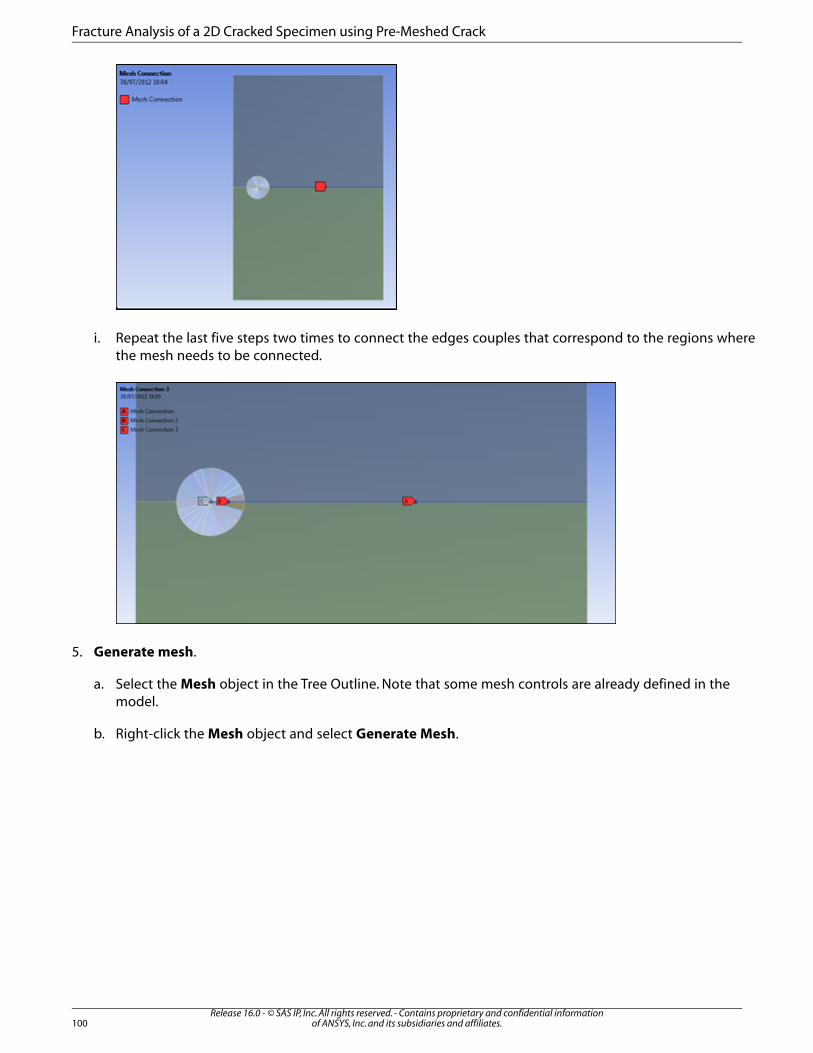
i. Repeat the last five steps two times to connect the edges couples that correspond to the regions wherethe mesh needs to be connected.
5. Generate mesh.
a. Select the Mesh object in the Tree Outline. Note that some mesh controls are already defined in themodel.
b. Right-click the Mesh object and select Generate Mesh.
Release 16.0 - © SAS IP, Inc. All rights reserved. - Contains proprietary and confidential informationof ANSYS, Inc. and its subsidiaries and affiliates.100
Fracture Analysis of a 2D Cracked Specimen using Pre-Meshed Crack
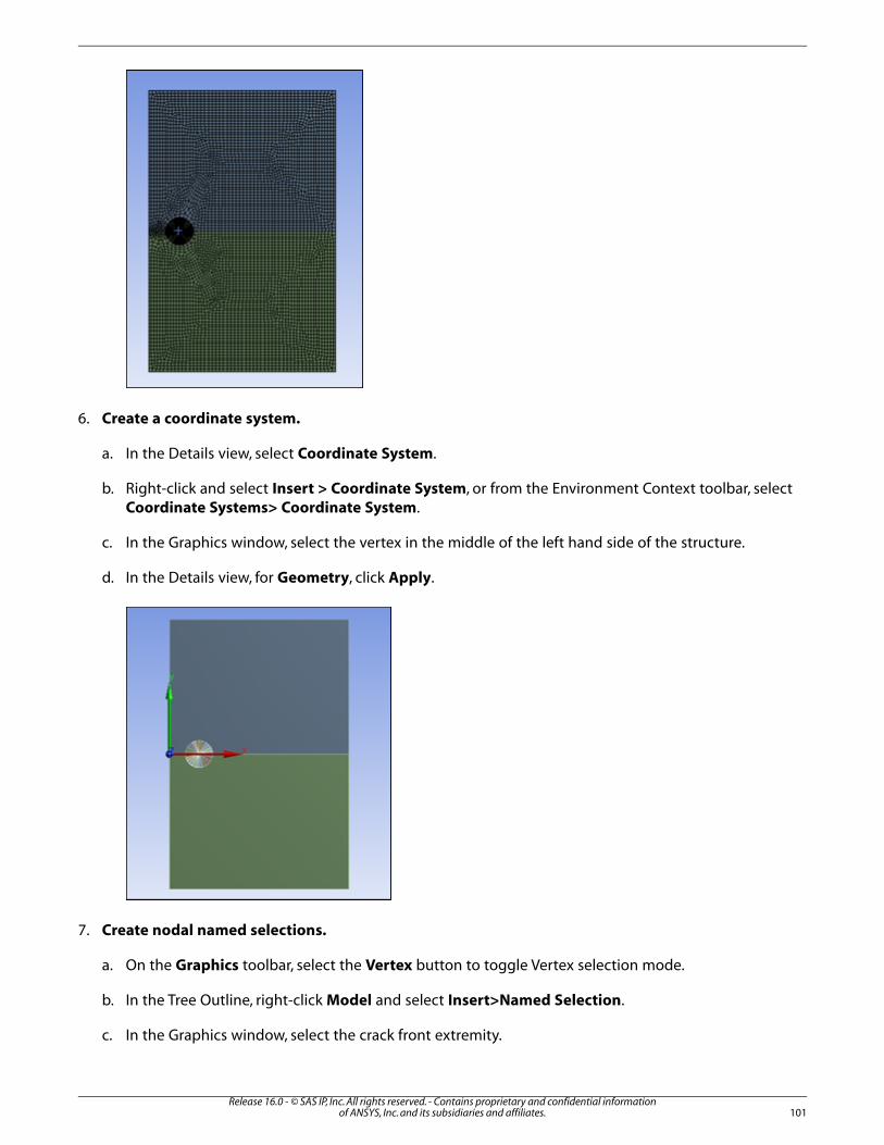
6. Create a coordinate system.
a. In the Details view, select Coordinate System.
b. Right-click and select Insert > Coordinate System, or from the Environment Context toolbar, selectCoordinate Systems> Coordinate System.
c. In the Graphics window, select the vertex in the middle of the left hand side of the structure.
d. In the Details view, for Geometry, click Apply.
7. Create nodal named selections.
a. On the Graphics toolbar, select the Vertex button to toggle Vertex selection mode.
b. In the Tree Outline, right-click Model and select Insert>Named Selection.
c. In the Graphics window, select the crack front extremity.
101Release 16.0 - © SAS IP, Inc. All rights reserved. - Contains proprietary and confidential information
of ANSYS, Inc. and its subsidiaries and affiliates.

d. In the Details pane, for Geometry, click Apply.
The named selection is created for the selected vertex.
e. In the Tree Outline, under Named Selections, right-click the new named selection and select Rename.
f. Enter crack_front as the name.
g. Right-click the crack_front named selection and select Create Nodal Named Selection.
h. In the Tree Outline, under Named Selections, right-click the new named selection and select Rename.
i. Enter crack_node as the name.
8. Define the crack.
a. Insert a Pre-Meshed Crack object into the Tree by right-clicking the Fracture object and selecting Insert> Pre-Meshed Crack.
b. In the Details View, for Crack Front (Named Selection), select the crack_node nodal named selection.
c. For Coordinate System, select the coordinate system you previously defined.
d. For Solution Contours, set the value to 10.
e. Leave the Suppressed value set to No.
9. Apply loads.
a. From the Menu bar , choose Units> Metric (mm, kg, N, s, mV, mA).
b. In the Tree Outline, select Static Structural.
c. Right-click and select Insert>Displacement, or from the Environment Context toolbar, select Supports> Displacement.
d. In the Graphics toolbar, select the Edge button.
e. In the Graphics window, select the bottom edge.
Release 16.0 - © SAS IP, Inc. All rights reserved. - Contains proprietary and confidential informationof ANSYS, Inc. and its subsidiaries and affiliates.102
Fracture Analysis of a 2D Cracked Specimen using Pre-Meshed Crack
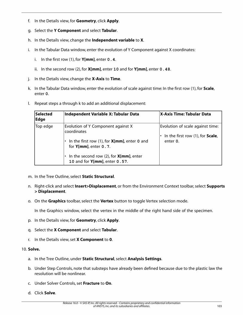
f. In the Details view, for Geometry, click Apply.
g. Select the Y Component and select Tabular.
h. In the Details view, change the Independent variable to X.
i. In the Tabular Data window, enter the evolution of Y Component against X coordinates:
i. In the first row (1), for Y[mm], enter 0.4.
ii. In the second row (2), for X[mm], enter 10 and for Y[mm], enter 0.48.
j. In the Details view, change the X-Axis to Time.
k. In the Tabular Data window, enter the evolution of scale against time: In the first row (1), for Scale,enter 0.
l. Repeat steps a through k to add an additional displacement:
X-Axis Time: Tabular DataIndependent Variable X: Tabular DataSelectedEdge
Evolution of scale against time:Evolution of Y Component against Xcoordinates
Top edge
• In the first row (1), for Scale,enter 0.• In the first row (1), for X[mm], enter 0 and
for Y[mm], enter 0.7.
• In the second row (2), for X[mm], enter10 and for Y[mm], enter 0.57.
m. In the Tree Outline, select Static Structural.
n. Right-click and select Insert>Displacement, or from the Environment Context toolbar, select Supports> Displacement.
o. On the Graphics toolbar, select the Vertex button to toggle Vertex selection mode.
In the Graphics window, select the vertex in the middle of the right hand side of the specimen.
p. In the Details view, for Geometry, click Apply.
q. Select the X Component and select Tabular.
r. In the Details view, set X Component to 0.
10. Solve.
a. In the Tree Outline, under Static Structural, select Analysis Settings.
b. Under Step Controls, note that substeps have already been defined because due to the plastic law theresolution will be nonlinear.
c. Under Solver Controls, set Fracture to On.
d. Click Solve.
103Release 16.0 - © SAS IP, Inc. All rights reserved. - Contains proprietary and confidential information
of ANSYS, Inc. and its subsidiaries and affiliates.
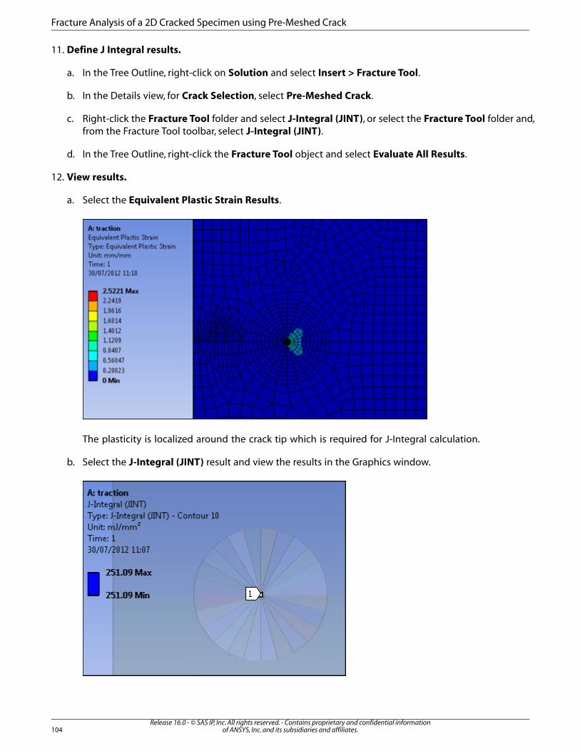
11. Define J Integral results.
a. In the Tree Outline, right-click on Solution and select Insert > Fracture Tool.
b. In the Details view, for Crack Selection, select Pre-Meshed Crack.
c. Right-click the Fracture Tool folder and select J-Integral (JINT), or select the Fracture Tool folder and,from the Fracture Tool toolbar, select J-Integral (JINT).
d. In the Tree Outline, right-click the Fracture Tool object and select Evaluate All Results.
12. View results.
a. Select the Equivalent Plastic Strain Results.
The plasticity is localized around the crack tip which is required for J-Integral calculation.
b. Select the J-Integral (JINT) result and view the results in the Graphics window.
Release 16.0 - © SAS IP, Inc. All rights reserved. - Contains proprietary and confidential informationof ANSYS, Inc. and its subsidiaries and affiliates.104
Fracture Analysis of a 2D Cracked Specimen using Pre-Meshed Crack

c. View the Graph window and the tabular data for each result. The tabular data display the J-Integralresults at the crack front node for each integration contour.
Note that the results converge after several contour integrations. J-Integral results start convergingwhen the integration contour is outside the plastic zone.
You have completed the fracture analysis and accomplished the overall objective for this tutorial.
End of tutorial.
105Release 16.0 - © SAS IP, Inc. All rights reserved. - Contains proprietary and confidential information
of ANSYS, Inc. and its subsidiaries and affiliates.

Release 16.0 - © SAS IP, Inc. All rights reserved. - Contains proprietary and confidential informationof ANSYS, Inc. and its subsidiaries and affiliates.106

Fracture Analysis of a Double Cantilever Beam (DCB) usingPre-Meshed Crack
Problem Description
The Double Cantilever Beam shown below is cracked at the center. This problem uses an importedmodel, already meshed, and then computes fracture parameters (energy release rates) using the VirtualCrack Close Technique (VCCT) on a static structural analysis to determine the impact of a catastrophicfailure to the structure.
Features Illustrated
• Importing a meshed model using Finite Element Modeler.
• Nodal named selections.
• Coordinate systems.
• Crack definition.
• Fracture Results
• Charting.
Procedure
1. Create a Finite Element Modeler (FEM) system.
a. Start ANSYS Workbench.
b. From the Toolbox, under Component System, drag a Finite Element Modeler system onto the ProjectSchematic.
107Release 16.0 - © SAS IP, Inc. All rights reserved. - Contains proprietary and confidential information
of ANSYS, Inc. and its subsidiaries and affiliates.

2. Import the meshed model.
Import a Mechanical APDL input file into Finite Modeler.
a. In the Finite Element Modeler schematic, right-click the Model cell and select Add Input Mesh >Browse.
b. In the Open dialog box, for Please select your model format, select Mechanical APDL Input (*.cdb).
c. Browse to open the file 3d_vcct. This file is available on the ANSYS Customer Portal; go to http://support.ansys.com/training.
d. Right-click the Model cell and select Properties to view the assembly mesh file you imported.
3. Establish a static structural analysis.
a. From the Toolbox, drag a Static Structural system onto the Project Schematic.
b. Drag the Model cell on the Finite Element Modeler schematic on to the Model cell of the StaticStructural system.
c. Right-click the Model cell on the Finite Element Modeler and select Update.
d. Right-click the Model cell of the Static Structural system and select Refresh.
4. Continue preparing the analysis in the Mechanical Application.
a. In the Static Structural schematic, right-click the Model cell, and then choose Edit. The MechanicalApplication opens and displays the model.
Note that the mesh is composed of linear elements, and VCCT is only applicable to linear elements
b. For convenience, use the Rotate toolbar button to manipulate the model so it displays as shown below.
Note
You can perform the same model manipulations by holding down the mouse wheelor middle button while dragging the mouse.
c. From the Menu bar , choose Units> Metric (m, kg, N, s, V, A) .
Release 16.0 - © SAS IP, Inc. All rights reserved. - Contains proprietary and confidential informationof ANSYS, Inc. and its subsidiaries and affiliates.108
Fracture Analysis of a Double Cantilever Beam (DCB) using Pre-Meshed Crack

5. Create a nodal named selection.
a. On the Graphics toolbar, select the Edge button to toggle Edge selection mode.
b. On the Graphics Options toolbar, select the Wireframe button to toggle wireframe mode.
c. In the Tree Outline, right-click Model and select Insert>Named Selection.
d. In the Graphics window, select the crack front edge.
e. In the Details pane, for Geometry, click Apply.
The named selection is created for the selected edge.
f. In the Tree Outline, under Named Selections, right-click the new named selection and select Rename.
g. Enter crack_front as the name.
h. Right-click the crack_front named selection and select Create Nodal Named Selection.
i. In the Tree Outline, under Named Selections, right-click the new named selection and select Rename.
j. Enter crack_nodes as the name.
6. Create a coordinate system with a Y-axis aligned to crack normal.
a. In the Details view, select Coordinate System.
b. In the Graphics window, select the edge on the open side of the crack.
c. Right-click and select Insert > Coordinate System. The origin of the coordinate system should be onthe open side of the crack.
d. In the Details view, for Geometry, click Apply.
e. Under Principal Axis, for Axis, select Y.
f. For Define by, select Global Z Axis.
g. Leave all other values at their defaults.
7. Define the crack.
a. Select the Model object in the Tree Outline.
b. Insert a Fracture object into the Tree by right-clicking the Model object and selecting Insert > Fracture.
c. Insert a Pre-Meshed Crack object into the Tree by right-clicking the Fracture object and selecting Insert> Pre-Meshed Crack.
d. In the Details View, for Crack Front (Named Selection), select the crack_nodes nodal named selection.
e. For Coordinate System, select the coordinate system you defined.
f. Leave the Suppressed value set to No.
109Release 16.0 - © SAS IP, Inc. All rights reserved. - Contains proprietary and confidential information
of ANSYS, Inc. and its subsidiaries and affiliates.

8. Apply loads.
a. In the Tree Outline, select Static Structural.
b. Right-click and select Insert>Fixed Support, or from the Environment Context toolbar, select Supports> Fixed Support.
c. In the Graphics toolbar, select the Face button.
d. In the Graphics window, select the face on the closed side of the crack.
e. In the Details view, for Geometry, click Apply.
f. Right-click and select Insert>Displacement, or from the Environment Context toolbar, select Supports> Displacement.
g. In the Graphics toolbar, select the Edge button.
h. In the Graphics window, select the top edge on the open side of the crack.
i. In the Details view, for Geometry, click Apply.
j. Select the Z Component and select Tabular.
k. In the second row (2), for Z[m], enter 5.e-003.
l. Right-click and select Insert>Displacement, or from the Environment Context toolbar, select Supports> Displacement.
m. In the Graphics window, select the bottom edge on the open side of the crack.
n. In the Details view, for Geometry, click Apply.
o. Select the Z Component and select Tabular.
p. In the second row (2), for Z[m], enter -5.e-003.
Release 16.0 - © SAS IP, Inc. All rights reserved. - Contains proprietary and confidential informationof ANSYS, Inc. and its subsidiaries and affiliates.110
Fracture Analysis of a Double Cantilever Beam (DCB) using Pre-Meshed Crack

9. Define results.
a. In the Tree Outline, right-click on Solution and select Insert > Fracture Tool.
b. In the Details view, for Crack Selection, select Pre-Meshed Crack.
c. Right-click the Fracture Tool folder and select VCCT Results > VCCT (G1), or select the Fracture Toolfolder and, from the Fracture Tool toolbar, select VCCT Results > VCCT (G1).
d. Also add the VCCT (G2), VCCT (G3), and VCCT (GT) results.
10. Solve.
a. In the Tree Outline, under Static Structural, select Analysis Settings.
b. Under Solver Controls, set Fracture to On.
c. Click Solve.
11. View results.
a. Select each result and view the results in the Graphics window.
111Release 16.0 - © SAS IP, Inc. All rights reserved. - Contains proprietary and confidential information
of ANSYS, Inc. and its subsidiaries and affiliates.
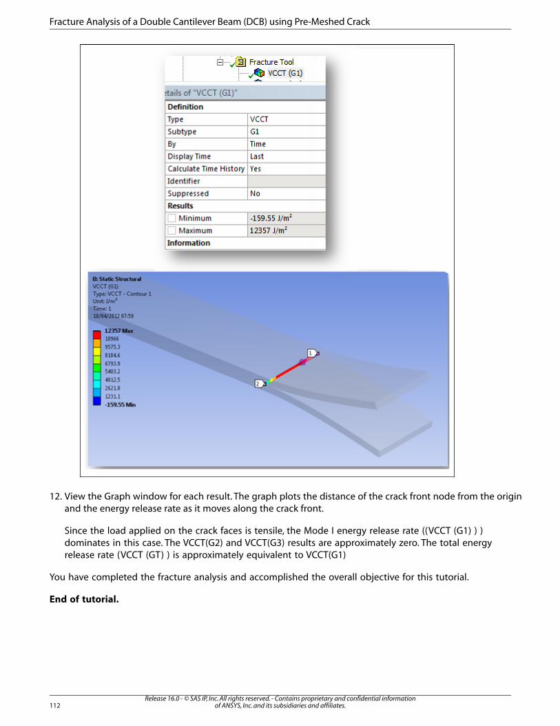
12. View the Graph window for each result. The graph plots the distance of the crack front node from the originand the energy release rate as it moves along the crack front.
Since the load applied on the crack faces is tensile, the Mode I energy release rate ((VCCT (G1) ) )dominates in this case. The VCCT(G2) and VCCT(G3) results are approximately zero. The total energyrelease rate (VCCT (GT) ) is approximately equivalent to VCCT(G1)
You have completed the fracture analysis and accomplished the overall objective for this tutorial.
End of tutorial.
Release 16.0 - © SAS IP, Inc. All rights reserved. - Contains proprietary and confidential informationof ANSYS, Inc. and its subsidiaries and affiliates.112
Fracture Analysis of a Double Cantilever Beam (DCB) using Pre-Meshed Crack
Fracture Analysis of an X-Joint Problem with Surface Flaw usingInternally Generated Crack Mesh
Problem Description
In this problem, a semi-elliptical crack is inserted at the tubular joint of the structure. Then crack meshis generated on the defined crack and fracture parameters based on Stress Intensity Factors (SIFS) arecomputed and post-processed.
Features Illustrated
• Importing geometry
• Nodal named selections.
• Coordinate systems.
• Crack definition.
• Fracture Results.
• Charting.
Procedure
1. Establish a static structural analysis.
a. Start ANSYS Workbench.
b. From the Toolbox, drag a Static Structural system onto the Project Schematic.
2. Import the model.
a. In the Static Structural schematic, right-click the Geometry cell and select Import Geometry > Browse.
b. Browse to open the file X_Joint.agdb. This file is available on the ANSYS Customer Portal; go to http://support.ansys.com/training.
3. Prepare the analysis in the Mechanical Application.
a. In the Static Structural schematic, right-click the Model cell, and then choose Edit. The MechanicalApplication opens and displays the model.
b. For convenience, use the Rotate toolbar button to manipulate the model so it displays as shown below.
113Release 16.0 - © SAS IP, Inc. All rights reserved. - Contains proprietary and confidential information
of ANSYS, Inc. and its subsidiaries and affiliates.

Note
You can perform the same model manipulations by holding down the mouse wheelor middle button while dragging the mouse.
4. Generate mesh.
a. In the Tree Outline, right-click Mesh and select Insert>Method.
b. In the Graphics window, select the body.
c. In the Details view, for Geometry, click Apply.
d. For Method, select Tetrahedrons.
This method is required for crack mesh generation.
e. In the Tree Outline, select the Mesh object.
f. In the Details view, under Sizing, set the Relevance Center to Fine.
g. On the Graphics toolbar, select the Face button to toggle Face selection mode.
h. In the Tree Outline, right-click Mesh and select Insert>Sizing.
i. In the Graphics window, select the external filet.
Release 16.0 - © SAS IP, Inc. All rights reserved. - Contains proprietary and confidential informationof ANSYS, Inc. and its subsidiaries and affiliates.114
Fracture Analysis of an X-Joint Problem with Surface Flaw using Internally GeneratedCrack Mesh

j. In the Details view, for Geometry, click Apply.
k. For Element Size, enter 5e-3 m.
l. Right-click the Mesh object and select Generate Mesh.
5. Create a coordinate system.
a. In the Details view, select Coordinate System.
b. In the Graphics window, select the edge on the open side of the crack.
c. Right-click and select Insert > Coordinate System, or from the Environment Context toolbar, selectCoordinate Systems> Coordinate System.
d. In the Graphics window, select the vertex lying at the center of the filet face.
115Release 16.0 - © SAS IP, Inc. All rights reserved. - Contains proprietary and confidential information
of ANSYS, Inc. and its subsidiaries and affiliates.

e. In the Details view, for Geometry, click Apply.
f. Under Principal Axis, for Axis, select X.
g. For Define by, select Hit Point Normal.
h. In the Graphics window, click at the origin location of the coordinate system.
i. In the Details view, for Hit Point Normal, click Apply.
6. Define the crack.
a. Select the Model object in the Tree Outline.
b. Insert a Fracture object into the Tree by right-clicking the Model object and selecting Insert > Fracture.
c. Insert a Crack object into the Tree by right-clicking the Fracture object and selecting Insert > Crack.
d. On the Graphics toolbar, select the Body button to toggle Body selection mode.
e. In the Graphics window, select the body.
f. In the Details view, for Geometry, click Apply.
g. For Coordinate System, select the coordinate system you previously defined.
h. In addition, set the following options in the Details view:
18.4mm
Major Radius
Release 16.0 - © SAS IP, Inc. All rights reserved. - Contains proprietary and confidential informationof ANSYS, Inc. and its subsidiaries and affiliates.116
Fracture Analysis of an X-Joint Problem with Surface Flaw using Internally GeneratedCrack Mesh
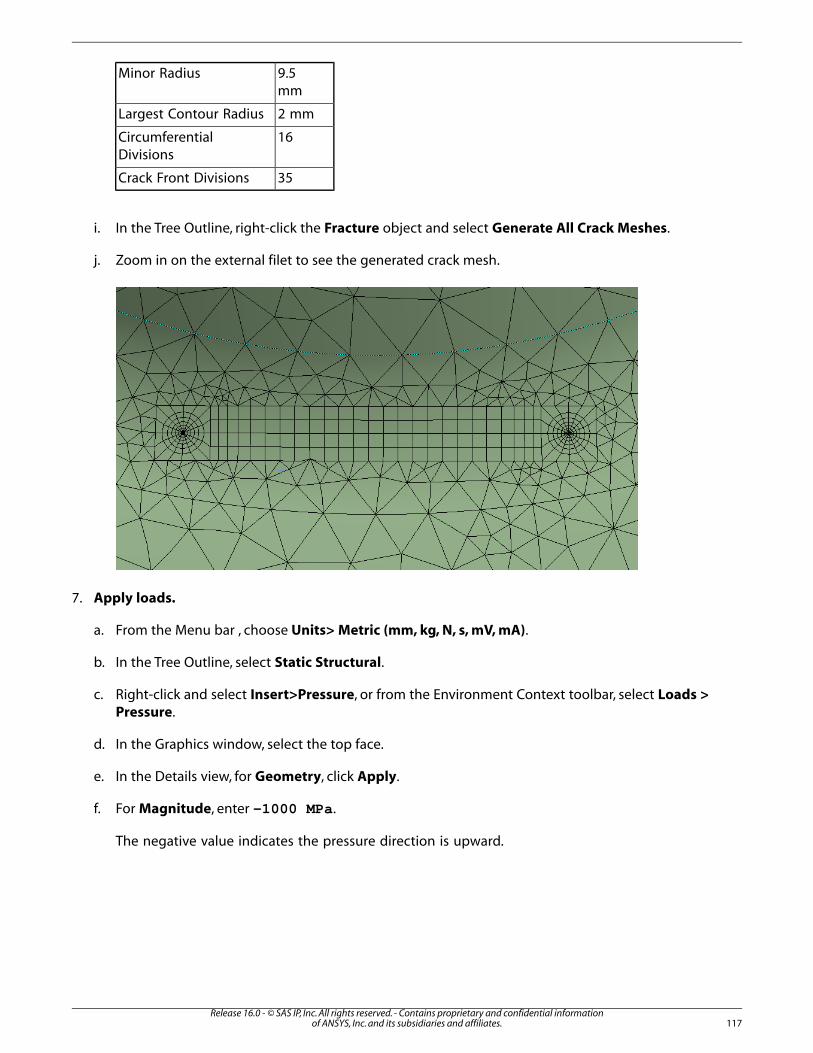
9.5mm
Minor Radius
2 mmLargest Contour Radius
16CircumferentialDivisions
35Crack Front Divisions
i. In the Tree Outline, right-click the Fracture object and select Generate All Crack Meshes.
j. Zoom in on the external filet to see the generated crack mesh.
7. Apply loads.
a. From the Menu bar , choose Units> Metric (mm, kg, N, s, mV, mA).
b. In the Tree Outline, select Static Structural.
c. Right-click and select Insert>Pressure, or from the Environment Context toolbar, select Loads >Pressure.
d. In the Graphics window, select the top face.
e. In the Details view, for Geometry, click Apply.
f. For Magnitude, enter -1000 MPa.
The negative value indicates the pressure direction is upward.
117Release 16.0 - © SAS IP, Inc. All rights reserved. - Contains proprietary and confidential information
of ANSYS, Inc. and its subsidiaries and affiliates.
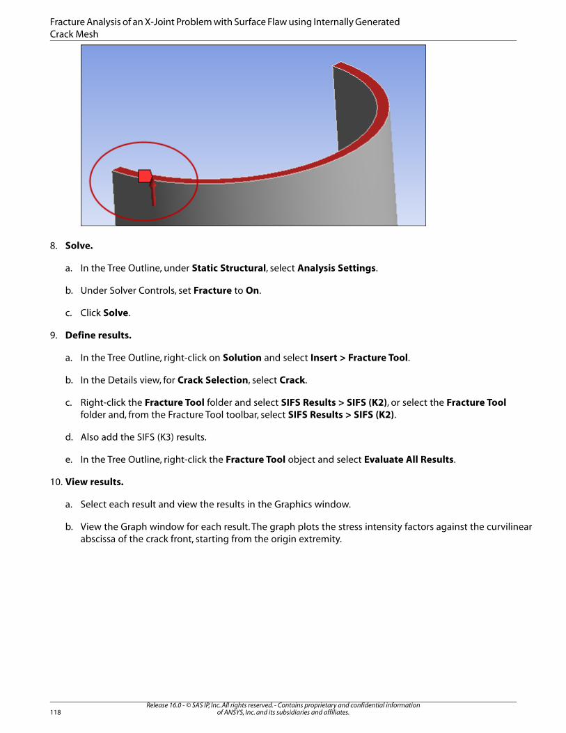
8. Solve.
a. In the Tree Outline, under Static Structural, select Analysis Settings.
b. Under Solver Controls, set Fracture to On.
c. Click Solve.
9. Define results.
a. In the Tree Outline, right-click on Solution and select Insert > Fracture Tool.
b. In the Details view, for Crack Selection, select Crack.
c. Right-click the Fracture Tool folder and select SIFS Results > SIFS (K2), or select the Fracture Toolfolder and, from the Fracture Tool toolbar, select SIFS Results > SIFS (K2).
d. Also add the SIFS (K3) results.
e. In the Tree Outline, right-click the Fracture Tool object and select Evaluate All Results.
10. View results.
a. Select each result and view the results in the Graphics window.
b. View the Graph window for each result. The graph plots the stress intensity factors against the curvilinearabscissa of the crack front, starting from the origin extremity.
Release 16.0 - © SAS IP, Inc. All rights reserved. - Contains proprietary and confidential informationof ANSYS, Inc. and its subsidiaries and affiliates.118
Fracture Analysis of an X-Joint Problem with Surface Flaw using Internally GeneratedCrack Mesh

Since the crack surface normal is nearly aligned with the tensile load, the Mode I stress intensityfactor (SIFS [K1]) dominates in this case. The SIFS (K2) and SIFS (K3) results show that Mode II andMode III slightly contribute.
You have completed the fracture analysis and accomplished the overall objective for this tutorial.
End of tutorial.
119Release 16.0 - © SAS IP, Inc. All rights reserved. - Contains proprietary and confidential information
of ANSYS, Inc. and its subsidiaries and affiliates.

Release 16.0 - © SAS IP, Inc. All rights reserved. - Contains proprietary and confidential informationof ANSYS, Inc. and its subsidiaries and affiliates.120

Using Finite Element Access to Resolve Overconstraint
Problem Description
This tutorial demonstrates the use of Finite Element (FE) types exposed in the Mechanical applicationby examining an analysis of a bracket assembly with contacts. This tutorial attempts to show the featuresrelated to FE types in the context of resolving an over-constraint issue in a Static Structural Analysis.
Features Demonstrated
• Create Node-based Named Selections
– Using Worksheet Criterion
– Using Node Selection Tool
• Scope FE (node-based) Boundary Conditions
• Display FE Connections
• Scope Results to FE Nodes
Setting Up the Analysis System
1. Create Static Structural Analysis.
a. Open ANSYS Workbench.
b. On the Workbench Project page, drag a Static Structural system from the Toolbox to the ProjectSchematic. The Project Schematic should appear as follows:
2. Assign Materials.
For this tutorial we will accept Structural Steel (typically the default material) for the model and addAluminum Alloy as a material option.
a. In the Static Structural schematic, right-click the Engineering Data cell and select Edit. The EngineeringData tab opens and displays Structural Steel as the default material.
121Release 16.0 - © SAS IP, Inc. All rights reserved. - Contains proprietary and confidential information
of ANSYS, Inc. and its subsidiaries and affiliates.

b. Right-click the box below Structural Steel, where it says "Click here to add new material" and selectEngineering Data Sources.
c. Select the General Materials check box and then click the Add button for Aluminum Alloy. A bookicon appears in the column next to the Add button (plus symbol) to indicate that the material is selected.
Release 16.0 - © SAS IP, Inc. All rights reserved. - Contains proprietary and confidential informationof ANSYS, Inc. and its subsidiaries and affiliates.122
Using Finite Element Access to Resolve Overconstraint
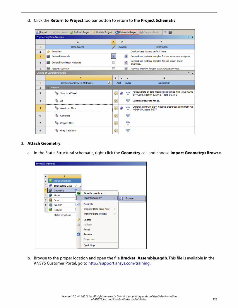
d. Click the Return to Project toolbar button to return to the Project Schematic.
3. Attach Geometry.
a. In the Static Structural schematic, right-click the Geometry cell and choose Import Geometry>Browse.
b. Browse to the proper location and open the file Bracket_Assembly.agdb. This file is available in theANSYS Customer Portal, go to http://support.ansys.com/training.
123Release 16.0 - © SAS IP, Inc. All rights reserved. - Contains proprietary and confidential information
of ANSYS, Inc. and its subsidiaries and affiliates.

Define the Model
1. Launch Mechanical by right-clicking the Model cell and then choosing Edit. (Tip: You can also double-click the cell to launch Mechanical).
2. Define Unit System: from the Menu bar , select Units> Metric (mm, kg, N, s, mV, mA).
3. Define Part Material and Create Named Selection.
a. For this model, all of the parts have been defined as Structural Steel. However, we want to change theMaterial type of the Clevis to Aluminum Alloy. To do this, first expand the Geometry object in the tree.
b. Select the Clevis object under Geometry. In the Details under the Material category, click the Struc-tural Steel option in the Assignment field to display the drop-down list. Change the material to Alu-minum Alloy.
c. Right-click on Clevis and select Create Named Selection. Enter the Selection Name "Clevis" and clickthe OK button.
Release 16.0 - © SAS IP, Inc. All rights reserved. - Contains proprietary and confidential informationof ANSYS, Inc. and its subsidiaries and affiliates.124
Using Finite Element Access to Resolve Overconstraint

The Selection Name window is shown below.
4. Define Connections.
a. Expand the Connections folder in the tree, and then expand the Contacts folder.
b. Right-click the Contacts folder and choose Renamed Based on Definition.
125Release 16.0 - © SAS IP, Inc. All rights reserved. - Contains proprietary and confidential information
of ANSYS, Inc. and its subsidiaries and affiliates.

Renaming is illustrated below.
Release 16.0 - © SAS IP, Inc. All rights reserved. - Contains proprietary and confidential informationof ANSYS, Inc. and its subsidiaries and affiliates.126
Using Finite Element Access to Resolve Overconstraint
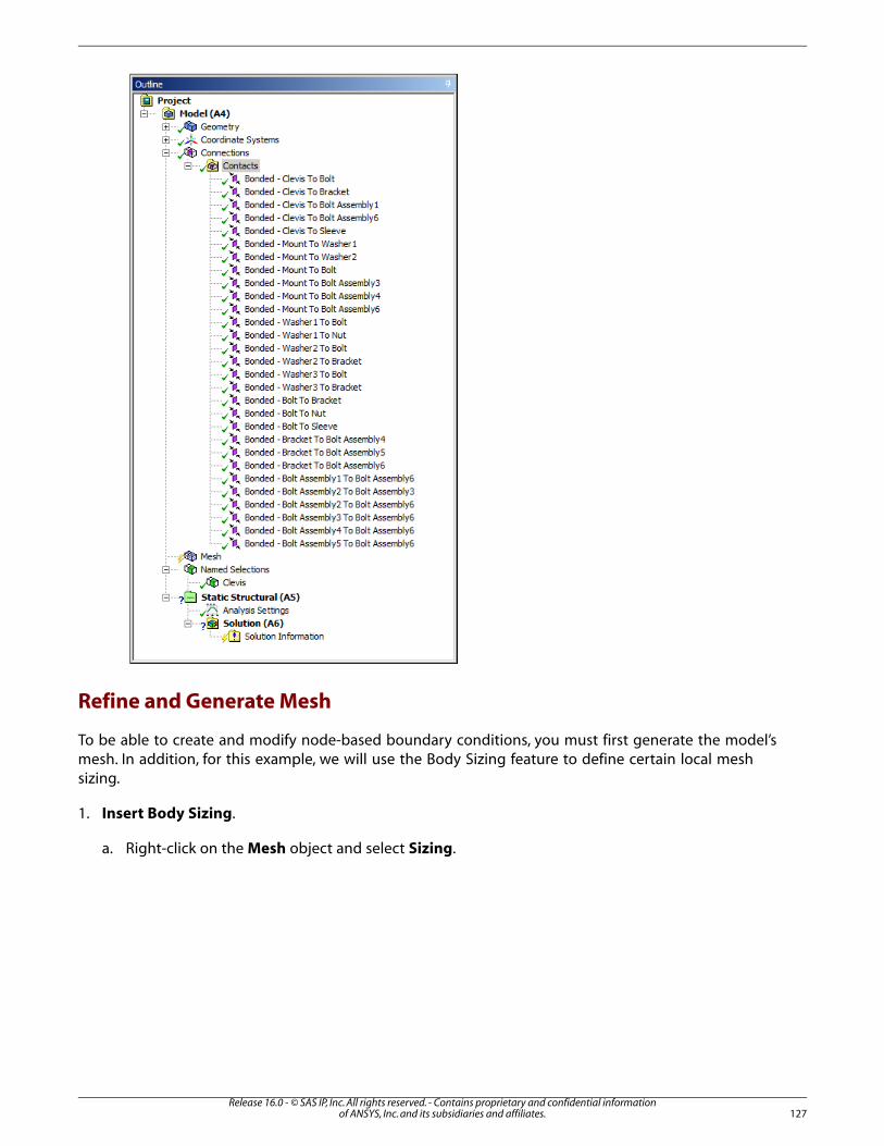
Refine and Generate Mesh
To be able to create and modify node-based boundary conditions, you must first generate the model’smesh. In addition, for this example, we will use the Body Sizing feature to define certain local meshsizing.
1. Insert Body Sizing.
a. Right-click on the Mesh object and select Sizing.
127Release 16.0 - © SAS IP, Inc. All rights reserved. - Contains proprietary and confidential information
of ANSYS, Inc. and its subsidiaries and affiliates.
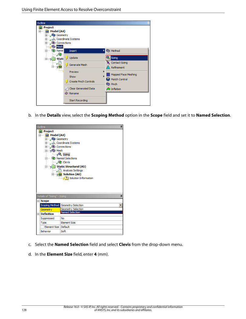
b. In the Details view, select the Scoping Method option in the Scope field and set it to Named Selection.
c. Select the Named Selection field and select Clevis from the drop-down menu.
d. In the Element Size field, enter 4 (mm).
Release 16.0 - © SAS IP, Inc. All rights reserved. - Contains proprietary and confidential informationof ANSYS, Inc. and its subsidiaries and affiliates.128
Using Finite Element Access to Resolve Overconstraint

e. Right-click the Body Sizing object and select Rename Based on Definition.
As illustrated here, the object is renamed.
129Release 16.0 - © SAS IP, Inc. All rights reserved. - Contains proprietary and confidential information
of ANSYS, Inc. and its subsidiaries and affiliates.

2. Generate Mesh: Right-click on the Mesh object select Generate Mesh.
The completed mesh is shown here.
Release 16.0 - © SAS IP, Inc. All rights reserved. - Contains proprietary and confidential informationof ANSYS, Inc. and its subsidiaries and affiliates.130
Using Finite Element Access to Resolve Overconstraint
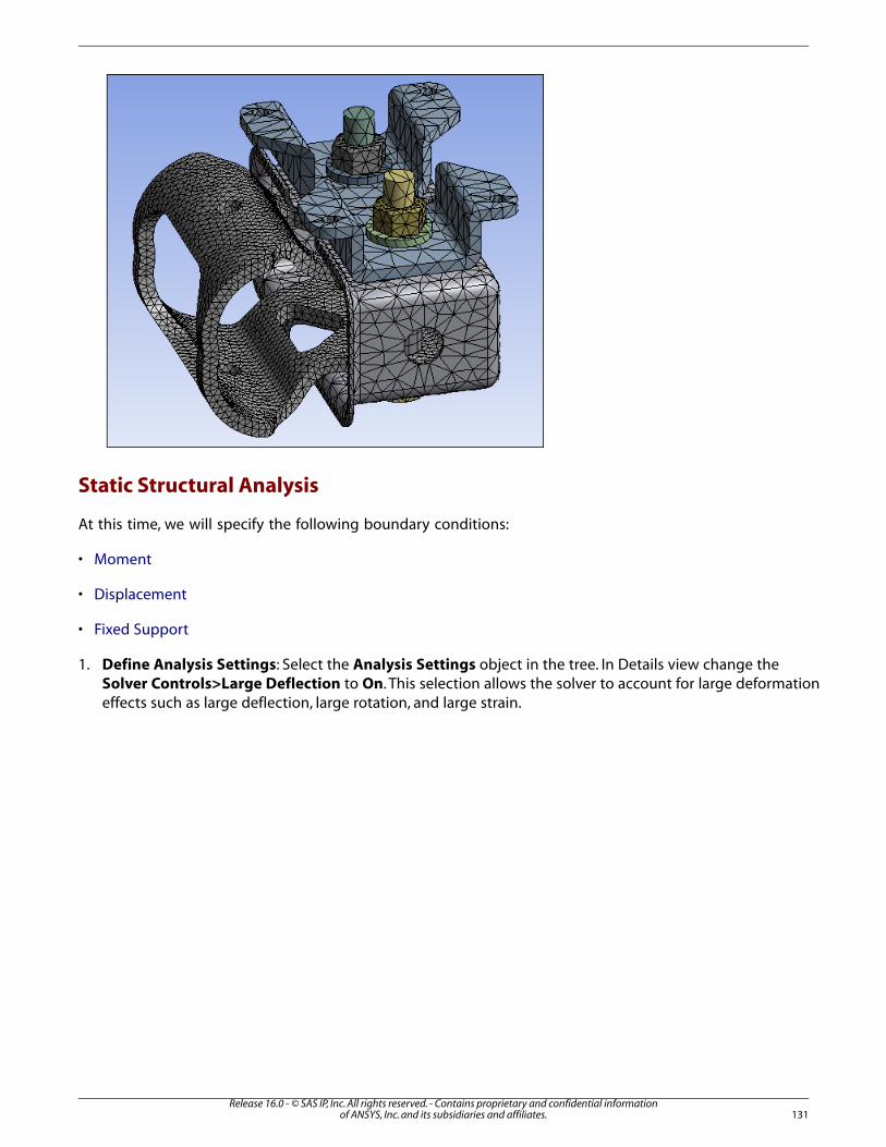
Static Structural Analysis
At this time, we will specify the following boundary conditions:
• Moment
• Displacement
• Fixed Support
1. Define Analysis Settings: Select the Analysis Settings object in the tree. In Details view change theSolver Controls>Large Deflection to On. This selection allows the solver to account for large deformationeffects such as large deflection, large rotation, and large strain.
131Release 16.0 - © SAS IP, Inc. All rights reserved. - Contains proprietary and confidential information
of ANSYS, Inc. and its subsidiaries and affiliates.

2. Insert a Moment Load.
a. Select the Static Structural object, right-click the mouse, and then choose Insert>Moment.
Release 16.0 - © SAS IP, Inc. All rights reserved. - Contains proprietary and confidential informationof ANSYS, Inc. and its subsidiaries and affiliates.132
Using Finite Element Access to Resolve Overconstraint

b. Select the inner face of the Clevis (1 Face) as illustrated here. In the Details for the Scope category,select the Geometry field and click Apply. Enter 1e5 N mm as the Magnitude and change the Beha-vior to Rigid.
3. Insert a Displacement and Fixed Support.
a. With the Moment object still highlighted, right-click the mouse and select Insert>Displacement.
133Release 16.0 - © SAS IP, Inc. All rights reserved. - Contains proprietary and confidential information
of ANSYS, Inc. and its subsidiaries and affiliates.

b. Select the inner face of the circular hole highlighted here. Make sure that the model is oriented asshown (note the direction of the bolts) and then click the Apply button in the Geometry field. Set thevalues of X Component, Y Component, and Z Component, to 0 mm.
c. Finally, let’s immobilize the assembly by specifying Fixed Supports on the faces illustrated below. Underthe Supports menu, select Fixed Support, select one of the faces, press and hold the Ctrl key, andthen select the remaining three faces. Once all of the faces are selected, click the Apply button in theGeometry field.
Release 16.0 - © SAS IP, Inc. All rights reserved. - Contains proprietary and confidential informationof ANSYS, Inc. and its subsidiaries and affiliates.134
Using Finite Element Access to Resolve Overconstraint

Results and Solution
This section outlines the steps to add result objects, solve your analysis, and review your results.
1. Specify Result Object and Solve.
a. Highlight the Solution object, select the Deformation Menu on the Solution Context Toolbar, andselect Total.
b. Right-click the Solution object and select Solve.
2. Review the Results.
a. Select the Total Deformation object. The solved model should display as follows:
135Release 16.0 - © SAS IP, Inc. All rights reserved. - Contains proprietary and confidential information
of ANSYS, Inc. and its subsidiaries and affiliates.

The bulk of the result displays in blue, indicating no deformations on the assembly. This cannotbe correct. In addition to that condition, the following Warning Messages display:
• Large deformation effects are active which may have invalidated some of your applied supports suchas displacement, cylindrical, frictionless, or compression only. Refer to Troubleshooting in the HelpSystem for more details.
• One or more MPC contact regions or remote boundary conditions may have conflicts with otherapplied boundary conditions or other contact regions. Refer to Troubleshooting in the Help Systemfor more details.
This second message indicates that one of the nodes is likely over-constrained.
You can graphically display FE Connections from the Solution Information object, as illustratedbelow. In the Details, specify the Display control as CE Based and the Display Type as Lines.As you can see there is an abundance of Constraint Equations.
Release 16.0 - © SAS IP, Inc. All rights reserved. - Contains proprietary and confidential informationof ANSYS, Inc. and its subsidiaries and affiliates.136
Using Finite Element Access to Resolve Overconstraint
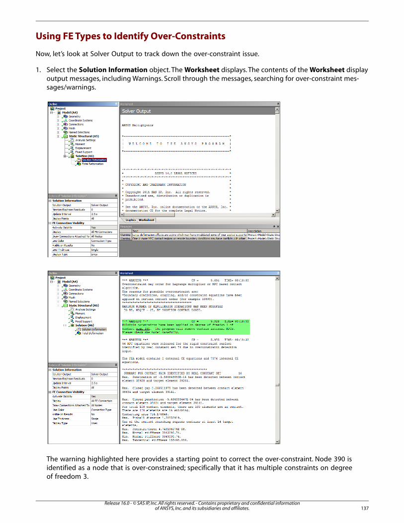
Using FE Types to Identify Over-Constraints
Now, let’s look at Solver Output to track down the over-constraint issue.
1. Select the Solution Information object. The Worksheet displays. The contents of the Worksheet displayoutput messages, including Warnings. Scroll through the messages, searching for over-constraint mes-sages/warnings.
The warning highlighted here provides a starting point to correct the over-constraint. Node 390 isidentified as a node that is over-constrained; specifically that it has multiple constraints on degreeof freedom 3.
137Release 16.0 - © SAS IP, Inc. All rights reserved. - Contains proprietary and confidential information
of ANSYS, Inc. and its subsidiaries and affiliates.

FE access makes it possible to select a single node using the Node ID. That is, Mechanical allows usto create a Named Selection that consists of Node 390 so we can that identify it specifically andview it graphically.
2. Select the Named Selections object and then click the Named Selection button on the toolbar. A Selectionobject is generated. In the Details for the Selection object, change the Scoping Method to Worksheet.The Worksheet view automatically displays.
Release 16.0 - © SAS IP, Inc. All rights reserved. - Contains proprietary and confidential informationof ANSYS, Inc. and its subsidiaries and affiliates.138
Using Finite Element Access to Resolve Overconstraint
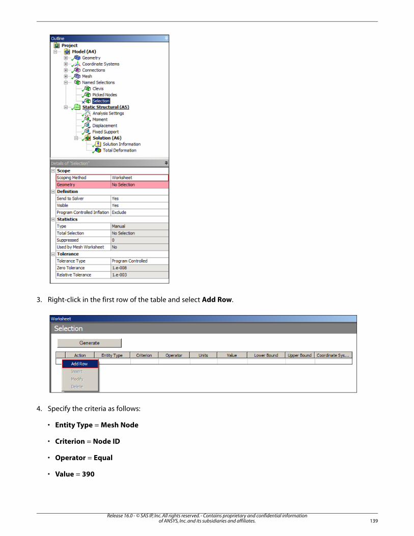
3. Right-click in the first row of the table and select Add Row.
4. Specify the criteria as follows:
• Entity Type = Mesh Node
• Criterion = Node ID
• Operator = Equal
• Value = 390
139Release 16.0 - © SAS IP, Inc. All rights reserved. - Contains proprietary and confidential information
of ANSYS, Inc. and its subsidiaries and affiliates.
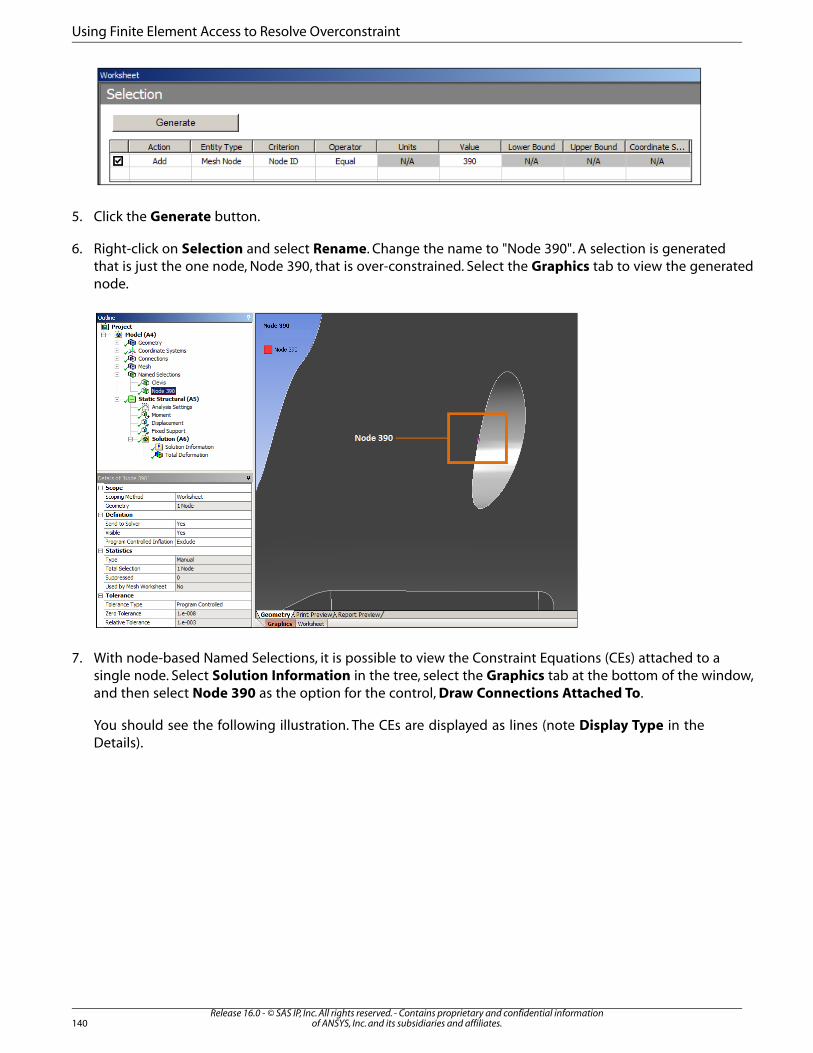
5. Click the Generate button.
6. Right-click on Selection and select Rename. Change the name to "Node 390". A selection is generatedthat is just the one node, Node 390, that is over-constrained. Select the Graphics tab to view the generatednode.
7. With node-based Named Selections, it is possible to view the Constraint Equations (CEs) attached to asingle node. Select Solution Information in the tree, select the Graphics tab at the bottom of the window,and then select Node 390 as the option for the control, Draw Connections Attached To.
You should see the following illustration. The CEs are displayed as lines (note Display Type in theDetails).
Release 16.0 - © SAS IP, Inc. All rights reserved. - Contains proprietary and confidential informationof ANSYS, Inc. and its subsidiaries and affiliates.140
Using Finite Element Access to Resolve Overconstraint

The Display Type specified as Points is illustrated below. You can see Node 390 as well as all ofthe other nodes used to calculate CEs. All nodes other than Node 390 are hollow. This indicates thateach node is connected to Node 390.
In addition, the Visible on Results control has been set to Yes. This facilitates the display of thecontour results for the Total Deformation result and the CEs, also shown below.
Here is an illustration of the CEs while the Total Deformation object is selected.
141Release 16.0 - © SAS IP, Inc. All rights reserved. - Contains proprietary and confidential information
of ANSYS, Inc. and its subsidiaries and affiliates.
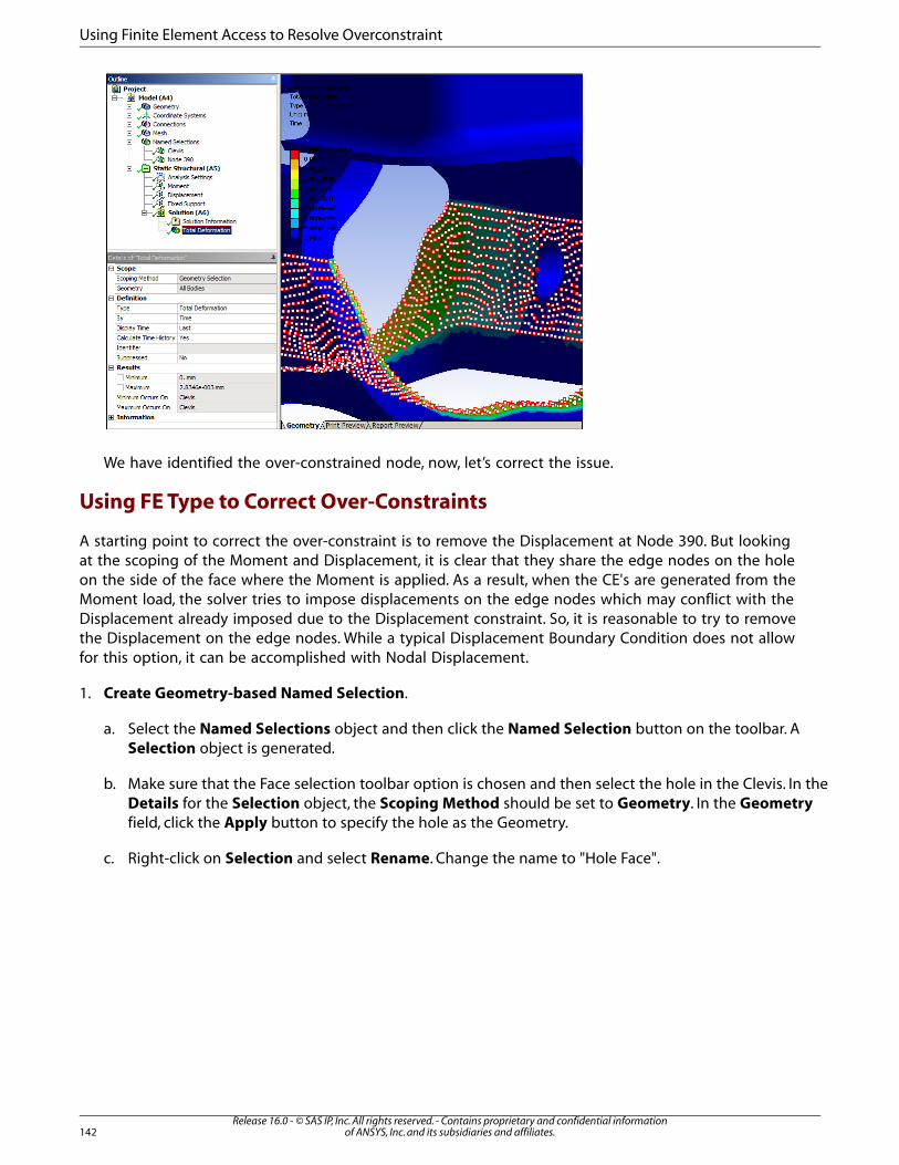
We have identified the over-constrained node, now, let’s correct the issue.
Using FE Type to Correct Over-Constraints
A starting point to correct the over-constraint is to remove the Displacement at Node 390. But lookingat the scoping of the Moment and Displacement, it is clear that they share the edge nodes on the holeon the side of the face where the Moment is applied. As a result, when the CE's are generated from theMoment load, the solver tries to impose displacements on the edge nodes which may conflict with theDisplacement already imposed due to the Displacement constraint. So, it is reasonable to try to removethe Displacement on the edge nodes. While a typical Displacement Boundary Condition does not allowfor this option, it can be accomplished with Nodal Displacement.
1. Create Geometry-based Named Selection.
a. Select the Named Selections object and then click the Named Selection button on the toolbar. ASelection object is generated.
b. Make sure that the Face selection toolbar option is chosen and then select the hole in the Clevis. In theDetails for the Selection object, the Scoping Method should be set to Geometry. In the Geometryfield, click the Apply button to specify the hole as the Geometry.
c. Right-click on Selection and select Rename. Change the name to "Hole Face".
Release 16.0 - © SAS IP, Inc. All rights reserved. - Contains proprietary and confidential informationof ANSYS, Inc. and its subsidiaries and affiliates.142
Using Finite Element Access to Resolve Overconstraint

2. Create Criterion-based Named Selection.
a. Select the Named Selections object and then click the Named Selection button on the toolbar. A newSelection object is generated.
b. Right-click on the new Selection object and select Rename. Change the name to "Hole Face Nodes".
c. In the Details for the Selection object, change the Scoping Method to Worksheet. The Worksheetview automatically displays.
d. Specify the criteria as illustrated here.
143Release 16.0 - © SAS IP, Inc. All rights reserved. - Contains proprietary and confidential information
of ANSYS, Inc. and its subsidiaries and affiliates.

e. Take a moment to review and consider the criterion you have defined and then click the Generatebutton.
3. Convert Edge to Nodes and Remove it from the Geometry. Now, let’s use a criterion-based Named Se-lection to create a Named Selection for the hole that subtracts (removes) the nodes of the hole’s edge.
a. Select the Named Selections object and then click the Named Selection button on the toolbar. ASelection object is generated.
b. Make sure that the Edge selection option is chosen and then select the edge of the hole. In the Detailsfor the Selection object, the Scoping Method should be set to Geometry. In the Geometry field, clickthe Apply button to specify the hole as the Geometry.
c. Right-click on Selection and select Rename. Change the name to "Hole Edge".
d. Select the Named Selections object and then click the Named Selection button on the toolbar. A newSelection object is generated.
e. Right-click on the new Selection object and select Rename. Change the name to "Hole Edge Nodes".
Release 16.0 - © SAS IP, Inc. All rights reserved. - Contains proprietary and confidential informationof ANSYS, Inc. and its subsidiaries and affiliates.144
Using Finite Element Access to Resolve Overconstraint

f. In the Details for the Selection object, change the Scoping Method to Worksheet. The Worksheetview automatically displays. Specify the criteria as illustrated here and then click the Generate button.
One more Named Selection is required. This Named Selection will remove the edge nodes fromthe hole nodes.
g. Select the Named Selections object and then click the Named Selection button on the toolbar. A newSelection object is generated.
h. Right-click on the new Selection object and select Rename. Change the name to "Hole Face MinusEdge".
i. In the Details for the Selection object, change the Scoping Method to Worksheet. Specify the criteriaas illustrated here and then click the Generate button.
We now have a node-based Named Selection that includes all of the nodes of the hole, minusthe nodes of the inner edge of the hole.
4. Suppress the existing Displacement: select the Displacement object, right-click the mouse, and selectSuppress. If desired, you could instead delete the load.
5. Create Nodal Displacement and Solve. Now let’s define the scope of the Nodal Displacement and re-solve the analysis.
145Release 16.0 - © SAS IP, Inc. All rights reserved. - Contains proprietary and confidential information
of ANSYS, Inc. and its subsidiaries and affiliates.

a. Select the Static Structural object, click the Direct FE menu in the toolbar, and then select NodalDisplacement.
b. Node-based boundary conditions can only be scoped to Named Selections. In the Details for the NodalDisplacement, specify Hole Face Minus Edge as the Named Selection and then specify each Com-ponent (X, Y, and Z) as 0.
c. Click the Solve button.
The solution should appear as shown here.
The Constraint Equations should appear with a uniform pattern, as illustrated here for the SolutionInformation object. And once again, the Visible on Results control has been set to Yes so thatyou can view Constraint Equations and contour results (make sure to select the Graphics tab).
Release 16.0 - © SAS IP, Inc. All rights reserved. - Contains proprietary and confidential informationof ANSYS, Inc. and its subsidiaries and affiliates.146
Using Finite Element Access to Resolve Overconstraint

6. Examine Equivalent Stresses. Now, let’s examine the Equivalent Stresses on the model.
a. Highlight the Solution object, right-click, and select Insert>Equivalent Stress.
b. Right-click the mouse and select Evaluate Results. The result should appear as illustrated here.
147Release 16.0 - © SAS IP, Inc. All rights reserved. - Contains proprietary and confidential information
of ANSYS, Inc. and its subsidiaries and affiliates.

A zero Displacement was applied and this is reflected in the above result.
c. Examine the stresses on the hole using direct node selection.
i. Graphically Select Nodes.
Select the Mesh object and then open the Select Type (Geometry/Mesh) menu and chooseSelect Mesh.
ii. Open the Select Mode menu and choose Box Select.
Release 16.0 - © SAS IP, Inc. All rights reserved. - Contains proprietary and confidential informationof ANSYS, Inc. and its subsidiaries and affiliates.148
Using Finite Element Access to Resolve Overconstraint

iii. Drag your cursor over the Clevis hole in a pattern similar to what is illustrated here to directly selectthe nodes in and around the hole.
iv. Right-click the mouse and select Named Selection. Enter "Stress Nodes" as the Selection Name.
149Release 16.0 - © SAS IP, Inc. All rights reserved. - Contains proprietary and confidential information
of ANSYS, Inc. and its subsidiaries and affiliates.
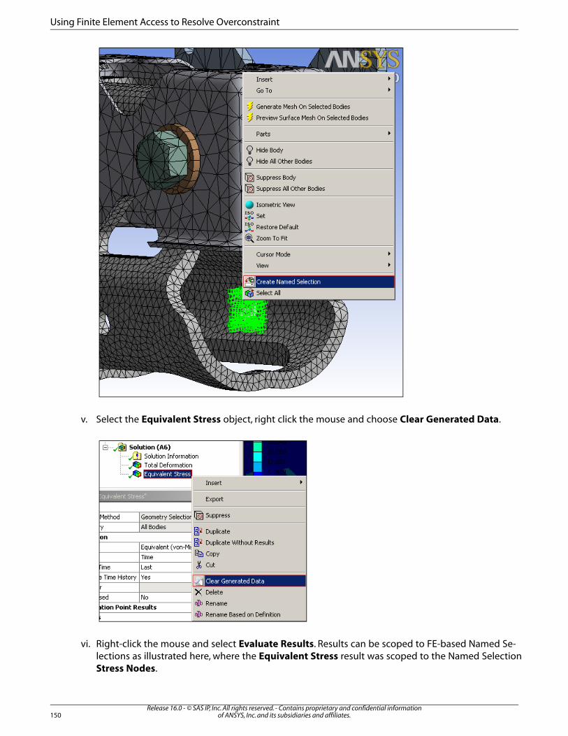
v. Select the Equivalent Stress object, right click the mouse and choose Clear Generated Data.
vi. Right-click the mouse and select Evaluate Results. Results can be scoped to FE-based Named Se-lections as illustrated here, where the Equivalent Stress result was scoped to the Named SelectionStress Nodes.
Release 16.0 - © SAS IP, Inc. All rights reserved. - Contains proprietary and confidential informationof ANSYS, Inc. and its subsidiaries and affiliates.150
Using Finite Element Access to Resolve Overconstraint

End of tutorial.
151Release 16.0 - © SAS IP, Inc. All rights reserved. - Contains proprietary and confidential information
of ANSYS, Inc. and its subsidiaries and affiliates.

Release 16.0 - © SAS IP, Inc. All rights reserved. - Contains proprietary and confidential informationof ANSYS, Inc. and its subsidiaries and affiliates.152

Simple Pendulum using Rigid Dynamics and Nonlinear Bushing
This tutorial demonstrates the use of a nonlinear bushing to modify the behavior of a simple pendulum.
Features Demonstrated
• Nonlinear bushings
• Reference coordinate system
• Mobile coordinate system
Setting Up the Analysis System
1. Prepare the analysis system.
a. Browse to open the file NLBushingTuto.wbpz. A Rigid Dynamics system will populate the ProjectSchematic. This file is available on the ANSYS Customer Portal; go to http://support.ansys.com/training.
b. Right click the Model cell, and select Edit to open the Mechanical Application. The model shown belowwill open.
153Release 16.0 - © SAS IP, Inc. All rights reserved. - Contains proprietary and confidential information
of ANSYS, Inc. and its subsidiaries and affiliates.

2. Continue preparing the analysis in the Mechanical Application.
a. From the Menu bar , choose Units>Metric (mm, kg, N, s, mV, mA).
b. From the Menu bar , choose Units>Degrees.
3. Insert a new bushing.
a. In the Outline view, expand the Connections node, then select the Joints node.
b. In the Connections toolbar, expand the Body-Body drop-down menu, and select Bushing.
Release 16.0 - © SAS IP, Inc. All rights reserved. - Contains proprietary and confidential informationof ANSYS, Inc. and its subsidiaries and affiliates.154
Simple Pendulum using Rigid Dynamics and Nonlinear Bushing

4. Scope the bushing to the correct faces:
a. In the Outline view, select the new bushing to display the bushing Details View.
b. In the Details View, click to activate the Reference Scoping Method field, then select Named Selectionfrom the drop-down menu.
c. Click to highlight the Reference Component field, then select FACE from the drop-down menu.
d. In the Details View, click to activate the Mobile Scoping Method field, then select Named Selectionfrom the drop-down menu.
e. Click to highlight the Mobile Component field, then select FACE2 from the drop-down menu.
The bushing reference coordinate system should now be defined as shown below:
155Release 16.0 - © SAS IP, Inc. All rights reserved. - Contains proprietary and confidential information
of ANSYS, Inc. and its subsidiaries and affiliates.

Note that the pendulum axis of rotation is the Z-axis.
5. Add a nonlinear rotational stiffness to the Z axis
a. In the Outline View, highlight the new bushing, then toggle the Worksheet view.
b. In the bushing worksheet, right-click the last diagonal term of the stiffness matrix, and select Tabular.
Release 16.0 - © SAS IP, Inc. All rights reserved. - Contains proprietary and confidential informationof ANSYS, Inc. and its subsidiaries and affiliates.156
Simple Pendulum using Rigid Dynamics and Nonlinear Bushing
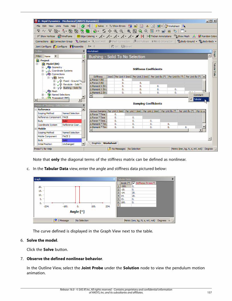
Note that only the diagonal terms of the stiffness matrix can be defined as nonlinear.
c. In the Tabular Data view, enter the angle and stiffness data pictured below:
The curve defined is displayed in the Graph View next to the table.
6. Solve the model.
Click the Solve button.
7. Observe the defined nonlinear behavior.
In the Outline View, select the Joint Probe under the Solution node to view the pendulum motionanimation.
157Release 16.0 - © SAS IP, Inc. All rights reserved. - Contains proprietary and confidential information
of ANSYS, Inc. and its subsidiaries and affiliates.

The pendulum should oscillate near its initial horizontal position due to the high stiffness enteredfor small angular displacements.
With joint rotation unsuppressed, a 20° rotation of the pendulum will occur at the beginning of theanalysis, and the pendulum should have free oscillation around the vertical axis.
End of tutorial.
Release 16.0 - © SAS IP, Inc. All rights reserved. - Contains proprietary and confidential informationof ANSYS, Inc. and its subsidiaries and affiliates.158
Simple Pendulum using Rigid Dynamics and Nonlinear Bushing

Track Roller Mechanism using Point on Curve Joints and Rigid BodyDynamics
This example problem demonstrates the use of a Rigid Dynamics analysis to examine the behavior ofa track-roller mechanism using point on curve joints.
In the example, the center point of an offset roller is placed directly onto a track edge to demonstratethe offset positioning capabilities of point on curve joints. While this model may not be entirely realistic,it clearly demonstrates the capabilities of the features highlighted.
Features Demonstrated
• Point on curve joints
• Reference coordinate system
• Mobile coordinate system
Setting Up the Analysis System
1. Prepare the analysis system.
a. Browse to open the file TrackRoller.mechdat. A Rigid Dynamics system will populate the ProjectSchematic. This file is available on the ANSYS Customer Portal; go to http://support.ansys.com/training.
b. Right click the Model cell, and select Edit to open the Mechanical Application. The model shown belowwill open.
159Release 16.0 - © SAS IP, Inc. All rights reserved. - Contains proprietary and confidential information
of ANSYS, Inc. and its subsidiaries and affiliates.

2. Insert a new joint.
In the Outline view, right-click the Connections node, then select Insert>Joint.
3. Define the new joint.
a. Select the new joint in the Outline to display the joint Details view.
b. In the Definition section of the Details view, click on the Connection Type field. The field becomesactive.
c. Select Body-Body from the Connection Type drop-down menu.
d. Click the Type field. The field becomes active.
e. Select Point on Curve from the Type drop-down menu.
4. Scope the new point on curve joint.
a. Use the edge selection tool to select an edge of the track to be used as the curve in the new point oncurve joint, as shown below.
Release 16.0 - © SAS IP, Inc. All rights reserved. - Contains proprietary and confidential informationof ANSYS, Inc. and its subsidiaries and affiliates.160
Track Roller Mechanism using Point on Curve Joints and Rigid Body Dynamics

b. In the Details view, click to activate the Reference Scope field.
c. Click Apply.
d. Use the face selection tool to select the face of the track to be used as the curve orientation surface, asshown below.
e. In the Details view, click to activate the Reference Curve Orientation Surface field.
f. Click Apply.
5. Define the reference coordinate system for the joint.
161Release 16.0 - © SAS IP, Inc. All rights reserved. - Contains proprietary and confidential information
of ANSYS, Inc. and its subsidiaries and affiliates.

a. In the Details view, click to activate the Reference Coordinate System field.
b. Configure the orientation of the reference coordinate system so that Z is the normal of the curve ori-entation surface and X is in the tangent of the curve. The correct orientation is show below.
c. Click Apply.
6. Select and configure the point used in the point on curve joint.
In this example, the center of the first roller (the circle selected below) will be selected as the pointfor the first joint. When creating a point on curve joint, the center of a selected geometric entity(i.e., a vertex, an edge, a surface, or a volume) is considered as the point. To specify a point:
a. Use the edge selection tool to select the outer edge of the roller, as shown below.
Release 16.0 - © SAS IP, Inc. All rights reserved. - Contains proprietary and confidential informationof ANSYS, Inc. and its subsidiaries and affiliates.162
Track Roller Mechanism using Point on Curve Joints and Rigid Body Dynamics

b. In the Details view of the joint, click to activate the Mobile Scope field.
c. Click Apply.
d. In the Details view, click to activate the Mobile Initial Position field.
e. Select Override from the Initial Position drop-down menu.
The Override option is necessary because the center point of the roller is offset from thetrack edge. If the Initial Position value of the mobile coordinate system is left to the defaultvalue, Unchanged, the reference coordinate system and mobile coordinate system are as-sumed to be coincident.
7. Define the mobile coordinate system for the joint.
The center of the roller face will be used as the origin in this model. The orientations of the referencecoordinate system and mobile coordinate system must be the same, or the point on curve joint willnot work properly. To define the mobile coordinate system:
a. In the joint Details view, click to activate the Mobile Coordinate System field.
b. Select the edge of the roller using the edge selection tool. By default, this will configure the mobilecoordinate system so that is corresponds to the reference coordinate system.
c. Ensure that both coordinate systems align as shown below, then click Apply.
163Release 16.0 - © SAS IP, Inc. All rights reserved. - Contains proprietary and confidential information
of ANSYS, Inc. and its subsidiaries and affiliates.

8. Create point of curve joint for the remaining rollers.
Create three more point on curve joints, one for each additional roller, and define them in a similarmanner as described in Step 3 through Step 7. Be sure to select a different roller edge (as describedin Step 6) for each additional joint. The completed model and coordinate systems should be con-figured as shown in the model below.
9. Solve the model.
Release 16.0 - © SAS IP, Inc. All rights reserved. - Contains proprietary and confidential informationof ANSYS, Inc. and its subsidiaries and affiliates.164
Track Roller Mechanism using Point on Curve Joints and Rigid Body Dynamics
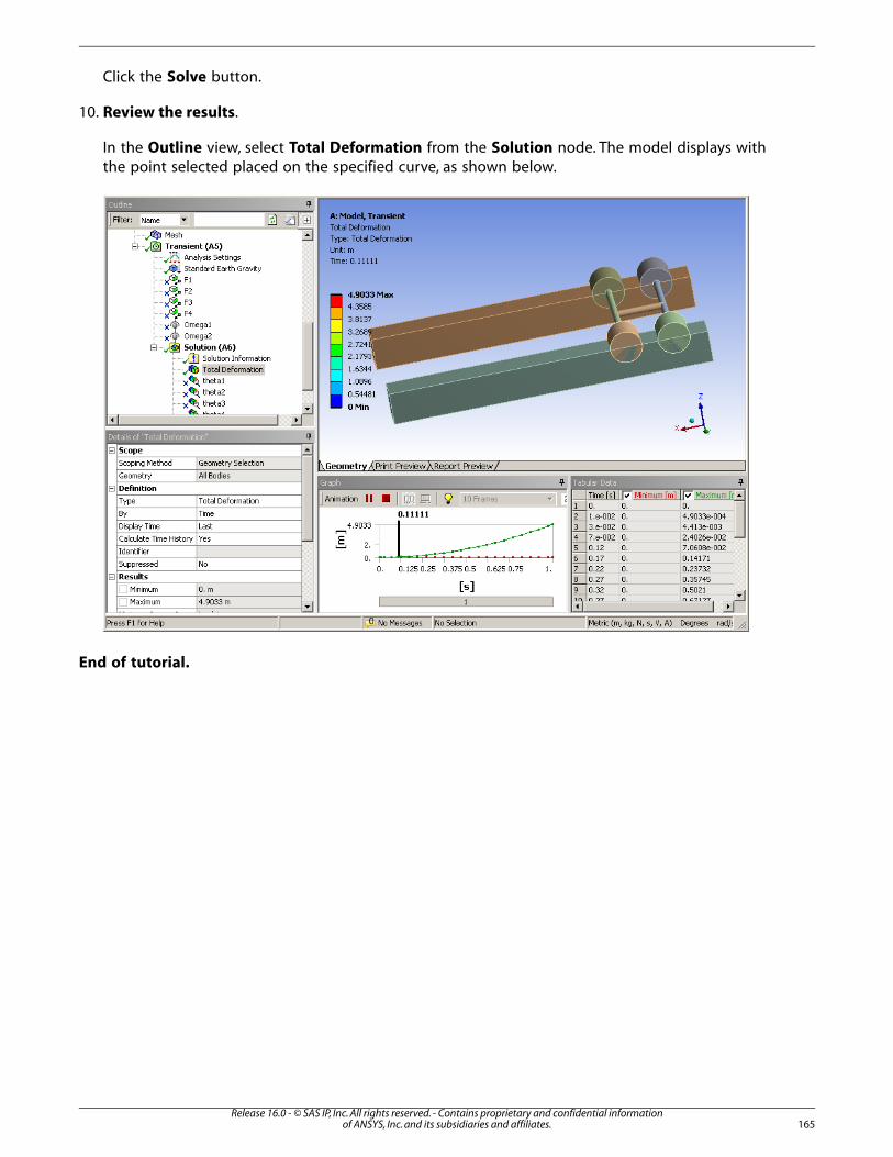
Click the Solve button.
10. Review the results.
In the Outline view, select Total Deformation from the Solution node. The model displays withthe point selected placed on the specified curve, as shown below.
End of tutorial.
165Release 16.0 - © SAS IP, Inc. All rights reserved. - Contains proprietary and confidential information
of ANSYS, Inc. and its subsidiaries and affiliates.

Release 16.0 - © SAS IP, Inc. All rights reserved. - Contains proprietary and confidential informationof ANSYS, Inc. and its subsidiaries and affiliates.166

IndexJjoints
point on curve, 159tutorial, 1
MMechanical tutorials, v
Nnonlinear bushing, 153
Ttutorials
Mechanical, v
167Release 16.0 - © SAS IP, Inc. All rights reserved. - Contains proprietary and confidential information
of ANSYS, Inc. and its subsidiaries and affiliates.

Release 16.0 - © SAS IP, Inc. All rights reserved. - Contains proprietary and confidential informationof ANSYS, Inc. and its subsidiaries and affiliates.168