ISSN 1055-1425

March 2005

This work was performed as part of the California PATH Program of the University of California, in cooperation with the State of California Business, Transportation, and Housing Agency, Department of Transportation; and the United States Department of Transportation, Federal Highway Administration.

The contents of this report reflect the views of the authors who are responsible for the facts and the accuracy of the data presented herein. The contents do not necessarily reflect the official views or policies of the State of California. This report does not constitute a standard, specification, or regulation.

Final Report for Task Order 4159

CALIFORNIA PATH PROGRAMINSTITUTE OF TRANSPORTATION STUDIESUNIVERSITY OF CALIFORNIA, BERKELEY

Anonymous Vehicle Tracking for Real-Time Freeway and Arterial Street Performance Measurement

UCB-ITS-PRR-2005-9California PATH Research Report

Stephen G. Ritchie, Seri Park, Cheol Oh, Shin-Ting (Cindy) Jeng, Andre TokUniversity of California, Irvine

CALIFORNIA PARTNERS FOR ADVANCED TRANSIT AND HIGHWAYS

California PATH

(Partners for Advanced Transit and Highways)

Task Order 4159 Final Report

Anonymous Vehicle Tracking for Real-Time Freeway and Arterial

Street Performance Measurement

Stephen G. Ritchie

Seri Park

Cheol Oh

Shin-Ting (Cindy) Jeng

Yeow Chern Andre Tok

Institute of Transportation Studies

University of California

Irvine, CA 92697-3600

January, 2005

ACKNOWLEDGEMENT

This work was performed as part of the California PATH Program of the University of California, in

cooperation with the State of California Business, Transportation and Housing Agency, Department of

Transportation; and the United States Department of Transportation, Federal Highway Administration.

The contents of this report reflect the views of the authors who are responsible for the facts and the

accuracy of the data presented herein. The contents do not necessarily reflect the official views or policies

of the State of California. This report does not constitute a standard, specification, or regulation.

The authors gratefully acknowledge the assistance of Steven Hilliard, Inductive Signature Technologies,

Inc., and Fred Yazdan, California Department of Transportation, in conducting this research.

ii

ABSTRACT

This research involved an important extension of existing field-implemented and tested PATH research by

the authors on individual vehicle reidentification, to develop methods for assessing freeway and arterial

(and transit) system performance for the Caltrans PeMS (Performance Measurement System). PeMS has

been adopted by Caltrans as the standard tool for assessing freeway system performance, but lacks

capabilities for assessing arterial and transit system performance, and strategies that combine freeways,

arterials and/or transit and commercial vehicle fleets. It was shown that the research methodology of this

project could directly address these limitations in PeMS. A systematic investigation was conducted of

anonymous vehicle tracking using existing inductive loop detectors on both freeway and arterial street

facilities combined with new, low-cost high-speed scanning detector cards (that were utilized by the

authors in PATH TO 4122) to meet the needs of PeMS. Both field data and microscopic simulation were

utilized in a major travel corridor setting, using the Paramics simulation model and field sites that were part

of the California ATMS (Advanced Transportation Management Systems) testbed network in Irvine,

California. The experience and insights of the research team obtained from extensive previous and current

PATH research on vehicle reidentification techniques for single roadway segments and signalized

intersections was used to investigate and develop methods for tracking individual vehicles (including

specified classes of vehicle such as buses and trucks) across multiple detector stations on a freeway and an

arterial street network to obtain real-time performance measurements (including dynamic or time-varying

origin-destination (OD) path flow information such as path travel time and volume). This study presented a

framework for studying the feasibility of an anonymous vehicle tracking system for real-time freeway and

arterial traffic surveillance and performance measurement. The potential feasibility of such an approach

was demonstrated by simulation experiments for both a freeway and a signalized arterial operated by

actuated traffic signal controls. Synthetic vehicle signatures were generated to evaluate the proposed

tracking algorithm under the simulation environment. The PARAMICS microscopic simulation model was

used to investigate the proposed vehicle tracking algorithm. The findings of this study can serve as a

logical and necessary precursor to possible field implementation of the proposed system in freeway and

arterial network. It is also believed that the proposed method for evaluating a traffic surveillance system

using microscopic simulation in this study can offer a valuable tool to operating agencies interested in real-

time congestion monitoring, traveler information, control, and system evaluation. Furthermore, the

automatic vehicle classification system developed in this study showed very encouraging results.

Keywords: vehicle signature, detector, sensor, inductive loop, vehicle classification, vehicle

reidentification, testbed, freeway, signalized intersection, level of service, detector card, search space

reduction, microscopic simulation

iii

EXECUTIVE SUMMARY

A new generation of Advanced Transportation Management and Information Systems (ATMIS) is now

widely under development, for applications in traveler information, route guidance, traffic control,

congestion monitoring, incident detection, and system evaluation, across extremely complex transportation

networks. However, the limitations, and often large errors, inherent in present point-based vehicle

surveillance systems greatly diminishes the ability of public agencies to effectively control, manage and

evaluate the performance of highway and transit systems, and to provide useful, timely and accurate travel

information to users. New types of travel data, in real-time, are essential for effective implementation and

performance assessment of ATMIS. In the past, such data were extremely difficult to obtain. To address

this need, there has recently been substantial interest in Europe and the United States, and particularly in

California, in implementing vehicle reidentification systems. Interest has initially focused on using the

extensive existing inductive loop infrastructure in California, while recognizing that some emerging

technologies such as video and laser detectors, the Global Positioning System (GPS) of satellites, and

automatic vehicle identification (AVI) systems involving on-board vehicle sensors/tags/transponders and

wireless vehicle-to vehicle and vehicle to roadside communications, may transition into practice in the

future.

Regardless of the traffic sensor technologies used, the California Department of Transportation (Caltrans)

has identified real-time travel time and origin-destination (OD) information as particularly important

outputs of such systems. Relatively inexpensive, anonymous individual vehicle tracking systems based on

the existing infrastructure of inductive loop detectors on freeway and arterial streets could be a particularly

cost-effective, immediately implementable solution, for the medium term and beyond. The vehicle

reidentification system developed by the authors in recent and current PATH research provides real-time

freeway and signalized intersection and arterial section or link traffic performance data, and potentially

network OD information such as vehicle paths and OD path travel times and volumes. Data such as these,

derived from individual vehicle tracking, form the basis for numerous real-time traffic performance

measures that can meet and exceed the needs of PeMS for assessment of freeway and arterial and transit

system performance.

However, all applications to date by the authors of the vehicle reidentification approach have been to

individual freeway, arterial or signalized intersection sites with only one upstream and downstream station

(and in the intersection case with three downstream stations for left, through and right vehicles). No

substantive studies have been undertaken of the ability of the system to operate effectively in a freeway or

arterial network, nor of the accuracy of OD information it would generate (except for the three destinations

represented by the left, through and right turn movements at an individual intersection). Although the

iv

potential for extension of this approach to network applications is very high, further feasibility study is

necessary before investing in actual network-wide implementation. This research conducted such a study,

using both field data and microscopic simulation of sites in the California ATMS Testbed in Irvine,

California.

A systematic investigation was conducted of anonymous vehicle tracking using existing inductive loop

detectors on both freeway and arterial street facilities combined with new, low-cost high-speed scanning

detector cards (that were utilized by the authors in PATH TO 4122) to meet the needs of PeMS. Both field

data and microscopic simulation were utilized in a major travel corridor setting, using the Paramics

simulation model and field sites that were part of the California ATMS (Advanced Transportation

Management Systems) testbed network in Irvine, California. The experience and insights of the research

team obtained from extensive previous and current PATH research on vehicle reidentification techniques

for single roadway segments and signalized intersections was used to investigate and develop methods for

tracking individual vehicles (including specified classes of vehicle such as buses and trucks) across

multiple detector stations on a freeway and an arterial street network to obtain real-time performance

measurements (including dynamic or time-varying origin-destination (OD) path flow information such as

path travel time and volume).

This study presented a framework for studying the feasibility of an anonymous vehicle tracking system for

real-time freeway and arterial traffic surveillance and performance measurement. The potential feasibility

of such an approach was demonstrated by simulation experiments for both a freeway and a signalized

arterial operated by actuated traffic signal controls. Synthetic vehicle signatures were generated to evaluate

the proposed tracking algorithm under the simulation environment. The PARAMICS microscopic

simulation model was used to investigate the proposed vehicle tracking algorithm. The findings of this

study can serve as a logical and necessary precursor to possible field implementation of the proposed

system in freeway and arterial network. It is also believed that the proposed method for evaluating a traffic

surveillance system using microscopic simulation in this study can offer a valuable tool to operating

agencies interested in real-time congestion monitoring, traveler information, control, and system

evaluation. Furthermore, the automatic vehicle classification system developed in this study showed very

encouraging results.

The findings of this study could be invaluable to Caltrans and other operating agencies interested in real-

time performance assessment of freeway and arterial street systems, and the implementation of such

capabilities in PeMS.

v

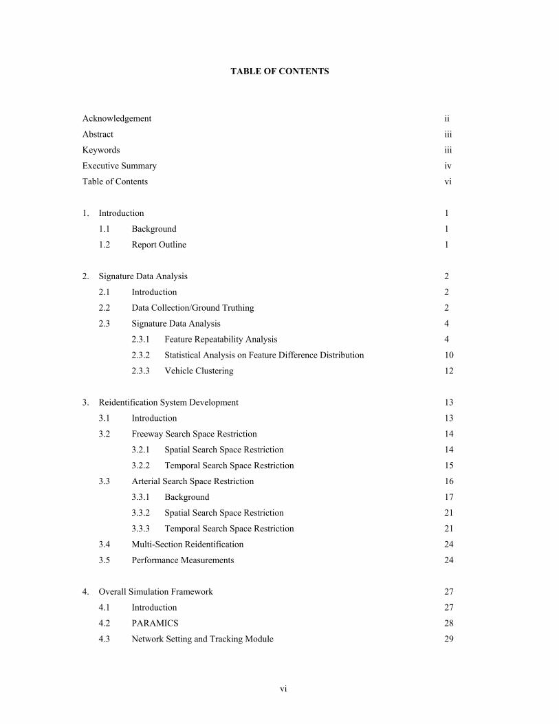
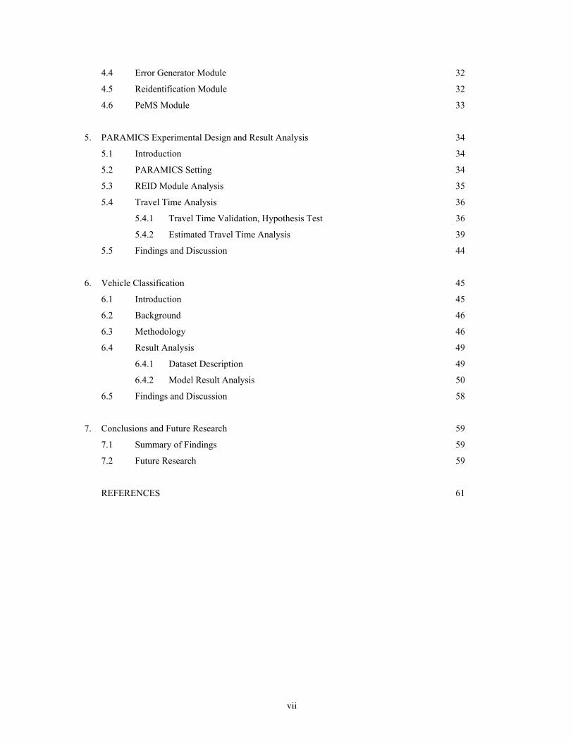
TABLE OF CONTENTS

Acknowledgement ii

Abstract iii

Keywords iii

Executive Summary iv

Table of Contents vi

1. Introduction 1

1.1 Background 1

1.2 Report Outline 1

2. Signature Data Analysis 2

2.1 Introduction 2

2.2 Data Collection/Ground Truthing 2

2.3 Signature Data Analysis 4

2.3.1 Feature Repeatability Analysis 4

2.3.2 Statistical Analysis on Feature Difference Distribution 10

2.3.3 Vehicle Clustering 12

3. Reidentification System Development 13

3.1 Introduction 13

3.2 Freeway Search Space Restriction 14

3.2.1 Spatial Search Space Restriction 14

3.2.2 Temporal Search Space Restriction 15

3.3 Arterial Search Space Restriction 16

3.3.1 Background 17

3.3.2 Spatial Search Space Restriction 21

3.3.3 Temporal Search Space Restriction 21

3.4 Multi-Section Reidentification 24

3.5 Performance Measurements 24

4. Overall Simulation Framework 27

4.1 Introduction 27

4.2 PARAMICS 28

4.3 Network Setting and Tracking Module 29

vi

vii

4.4 Error Generator Module 32

4.5 Reidentification Module 32

4.6 PeMS Module 33

5. PARAMICS Experimental Design and Result Analysis 34

5.1 Introduction 34

5.2 PARAMICS Setting 34

5.3 REID Module Analysis 35

5.4 Travel Time Analysis 36

5.4.1 Travel Time Validation, Hypothesis Test 36

5.4.2 Estimated Travel Time Analysis 39

5.5 Findings and Discussion 44

6. Vehicle Classification 45

6.1 Introduction 45

6.2 Background 46

6.3 Methodology 46

6.4 Result Analysis 49

6.4.1 Dataset Description 49

6.4.2 Model Result Analysis 50

6.5 Findings and Discussion 58

7. Conclusions and Future Research 59

7.1 Summary of Findings 59

7.2 Future Research 59

REFERENCES 61

Task Order 4122 - Anonymous Vehicle Tracking for Real-Time Freeway and Arterial Street Performance Measurement

CHAPTER 1 INTRODUCTION

1. Introduction

1.1 Background

One of the fundamental requirements to facilitate implementation of any Advanced Transportation

Management and Information System (ATMIS) is the development of a real-time traffic surveillance

system to produce reliable and accurate traffic performance measures. This report presents a new

framework for anonymous vehicle tracking that is capable of tracking individual vehicles by utilizing the

state – of – the art in detector technology. A systematic simulation investigation of the performance and

feasibility of anonymous vehicle tracking on freeways and signalized arterials using the PARAMICS

(PARAllel MICroscopic Simulation) simulation model is performed. Extensive study experience with

vehicle reidentification techniques on single roadway segments is used to investigate the performance

obtainable from tracking individual vehicles across multiple detector stations. The findings of this study

will serve as a logical and necessary precursor to possible field implementation of vehicle reidentification

techniques

1.2 Report Outline

In chapter 2, the analysis of real world vehicle signature data is discussed. This section will serve as basis

for the vehicle feature generation module in the microscopic simulation model. Chapter 3 presents

enhanced vehicle tracking algorithms for freeway and arterial sections. A multi-section vehicle tracking

scheme and possible elements for performance measurements are also discussed in this section. Simulation

settings, as well as each individual module inside the simulation, are presented in Chapter 4. Experimental

simulation design and results are described in chapter 5. An enhanced approach to vehicle classification is

presented in Chapter 6 . Finally, Chapter 7summarizes the conclusions of this research and directions for

future research.

1

CHAPTER 2 SIGNATURE DATA ANALYSIS

2.1 Introduction

Prior to using the simulation models for vehicle tracking, analysis of vehicle signature data should be

performed. This procedure is essential to obtain the input data for the simulated vehicle reidentification

system. Therefore, in this section, detailed analysis of vehicle signature data using a real world dataset

collected from Detector Testbed site was conducted for synthetic vehicle signature feature data generation.

Such analysis includes spatial repeatability and the error distribution of vehicle signature feature vectors.

This section will help to generate the input data for the vehicle reidentification algorithm that will be

implemented in the simulation model. The vehicle reidentification system and simulation model settings

will be discussed further in the following chapters.

2.2 Data Collection / Ground Truthing

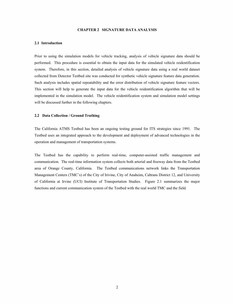
The California ATMS Testbed has been an ongoing testing ground for ITS strategies since 1991. The

Testbed uses an integrated approach to the development and deployment of advanced technologies in the

operation and management of transportation systems.

The Testbed has the capability to perform real-time, computer-assisted traffic management and

communication. The real-time information system collects both arterial and freeway data from the Testbed

area of Orange County, California. The Testbed communications network links the Transportation

Management Centers (TMC’s) of the City of Irivine, City of Anaheim, Caltrans District 12, and University

of California at Irvine (UCI) Institute of Transportation Studies. Figure 2.1 summarizes the major

functions and current communication system of the Testbed with the real world TMC and the field.

2

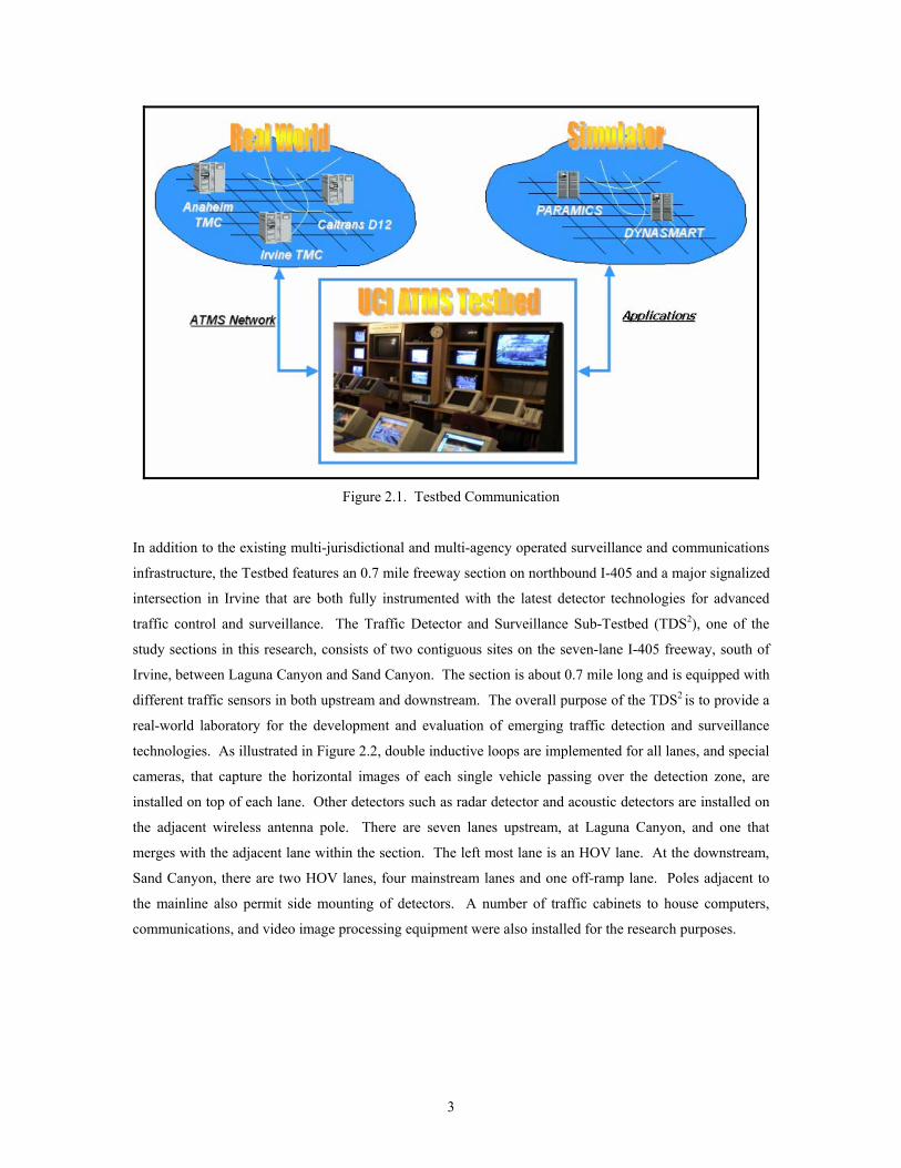
Figure 2.1. Testbed Communication

In addition to the existing multi-jurisdictional and multi-agency operated surveillance and communications

infrastructure, the Testbed features an 0.7 mile freeway section on northbound I-405 and a major signalized

intersection in Irvine that are both fully instrumented with the latest detector technologies for advanced

traffic control and surveillance. The Traffic Detector and Surveillance Sub-Testbed (TDS2), one of the

study sections in this research, consists of two contiguous sites on the seven-lane I-405 freeway, south of

Irvine, between Laguna Canyon and Sand Canyon. The section is about 0.7 mile long and is equipped with

different traffic sensors in both upstream and downstream. The overall purpose of the TDS2 is to provide a

real-world laboratory for the development and evaluation of emerging traffic detection and surveillance

technologies. As illustrated in Figure 2.2, double inductive loops are implemented for all lanes, and special

cameras, that capture the horizontal images of each single vehicle passing over the detection zone, are

installed on top of each lane. Other detectors such as radar detector and acoustic detectors are installed on

the adjacent wireless antenna pole. There are seven lanes upstream, at Laguna Canyon, and one that

merges with the adjacent lane within the section. The left most lane is an HOV lane. At the downstream,

Sand Canyon, there are two HOV lanes, four mainstream lanes and one off-ramp lane. Poles adjacent to

the mainline also permit side mounting of detectors. A number of traffic cabinets to house computers,

communications, and video image processing equipment were also installed for the research purposes.

3

Figure 2.2. Detector Testbed

The signature dataset used in this study was obtained from 15:00 to 15:20 PM on July 23rd, 2002. Detailed

description of the vehicle signatures can be found in many research studies by the authors (MOU 3008, TO

4122, Park et al 2004, Oh, S. et al 2002). Each upstream vehicle was manually matched to the

corresponding vehicle at downstream along with the corresponding vehicle class information. The dataset

contains about 2500 vehicles at each detection station. This data reduction result will serve as initial step

toward further analysis, such as feature repeatability test as well as feature difference distribution analysis

that are key issues for the error generator in simulation.

2.3 Signature Data Analysis

2.3.1 Feature Repeatability Analysis

Vehicle reidentification is a pattern recognition process based on the vehicle feature vectors from different

sites. Therefore, if signature variations that result in significant discrepancies between up and downstream

vehicle feature vectors do not exist, the algorithm would be capable of producing perfect vehicle signature

matching. However, in practice, because of the exogenous effects of environmental elements such as

physical loop installation, and entrance angle of a vehicle into the inductive field, vehicle signatures vary

4

from different detection stations. Therefore, investigation of such variations should be conducted to build

the basis for the synthetic vehicle signature generator in the simulation model. Detailed description on

vehicle feature vectors, vehicle specific feature vectors and traffic specific feature vectors, can be found

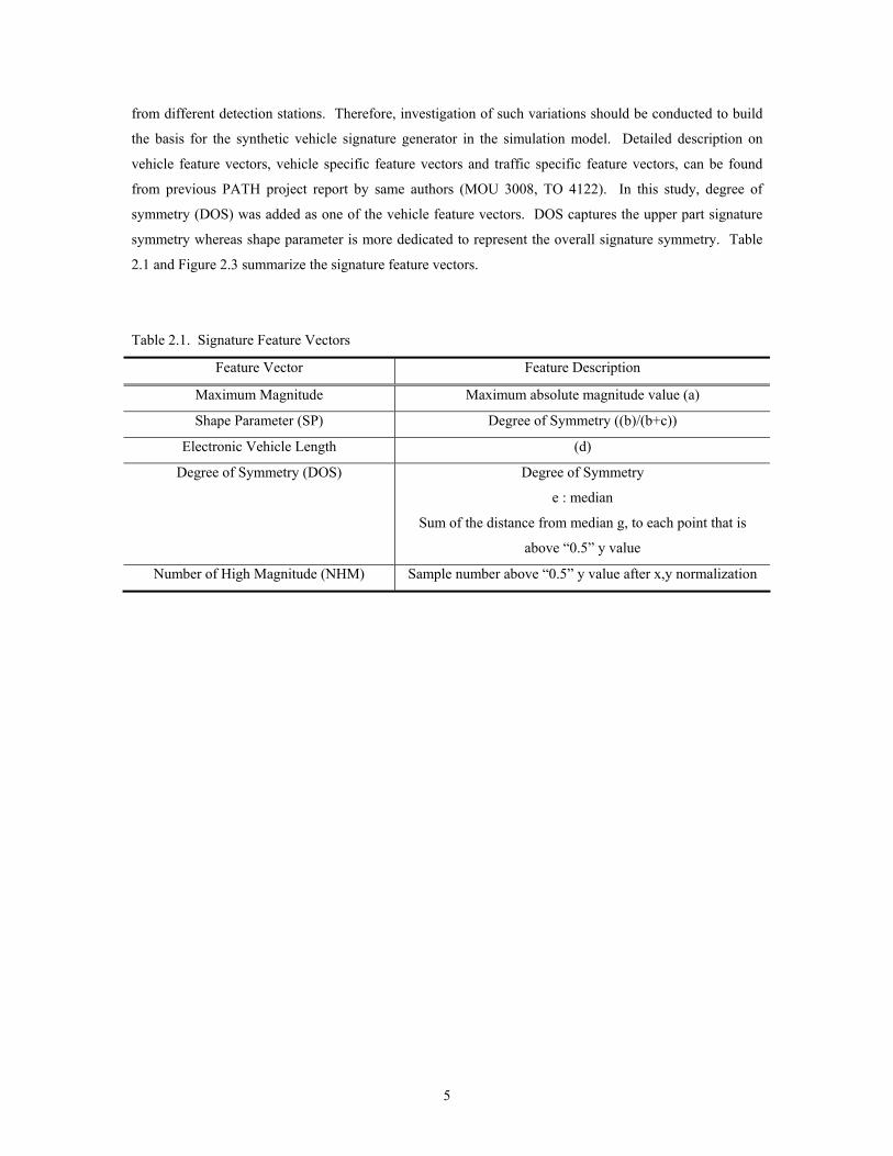
from previous PATH project report by same authors (MOU 3008, TO 4122). In this study, degree of

symmetry (DOS) was added as one of the vehicle feature vectors. DOS captures the upper part signature

symmetry whereas shape parameter is more dedicated to represent the overall signature symmetry. Table

2.1 and Figure 2.3 summarize the signature feature vectors.

Table 2.1. Signature Feature Vectors

Feature Vector Feature Description

Maximum Magnitude Maximum absolute magnitude value (a)

Shape Parameter (SP) Degree of Symmetry ((b)/(b+c))

Electronic Vehicle Length (d)

Degree of Symmetry (DOS) Degree of Symmetry

e : median

Sum of the distance from median g, to each point that is

above “0.5” y value

Number of High Magnitude (NHM) Sample number above “0.5” y value after x,y normalization

5

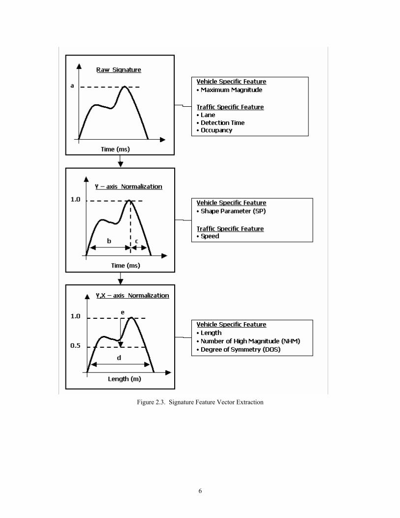
Figure 2.3. Signature Feature Vector Extraction

6

For the vehicle signature repeatability analysis, the average percentage error (APE) of each feature vector

was chosen as the criterion. Derivation of such index is as following:

si

iwhere

abs

FVAPE

FVFVFVAPE

s

i

i

down

i

down

i

up

ii

stationatFeature:

FeatureforErrorPercentageAverage:

100*)(

Average

−=

Analysis results are presented in Table 2.2, and among all the feature vectors analyzed, it is clear that the

vehicle length is the most reliable and repeatable one with the lowest average percentage error. This also

implies that the length feature will be the critical element to determine the system performance in the

reidentification model.

Table 2.2. Average Percentage Error

Feature Percentage Error in Feature Difference

Maximum Magnitude 22.97

Electronic Length 1.34

Shape Parameter (SP) 4.02

Number of High Magnitude (NHM) 2.09

Degree of Symmetry (DOS) 23.08

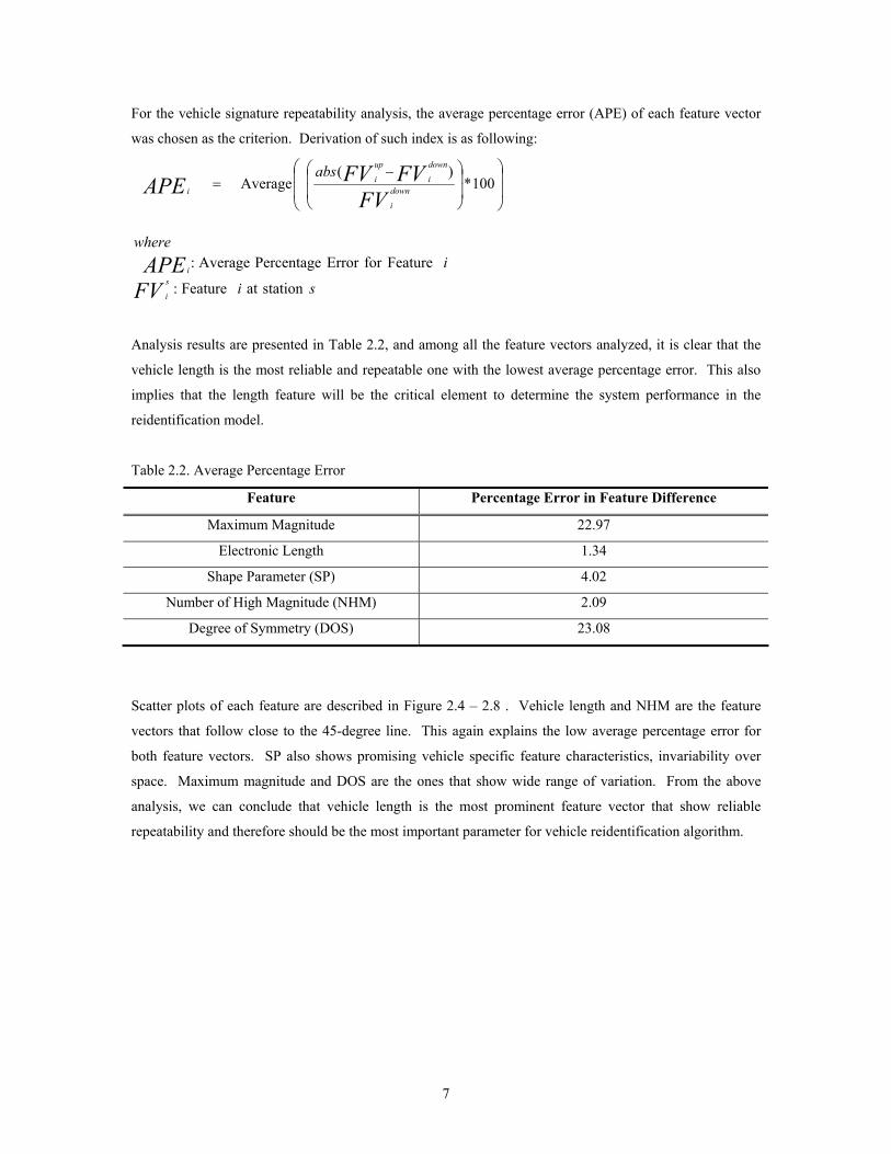
Scatter plots of each feature are described in Figure 2.4 – 2.8 . Vehicle length and NHM are the feature

vectors that follow close to the 45-degree line. This again explains the low average percentage error for

both feature vectors. SP also shows promising vehicle specific feature characteristics, invariability over

space. Maximum magnitude and DOS are the ones that show wide range of variation. From the above

analysis, we can conclude that vehicle length is the most prominent feature vector that show reliable

repeatability and therefore should be the most important parameter for vehicle reidentification algorithm.

7

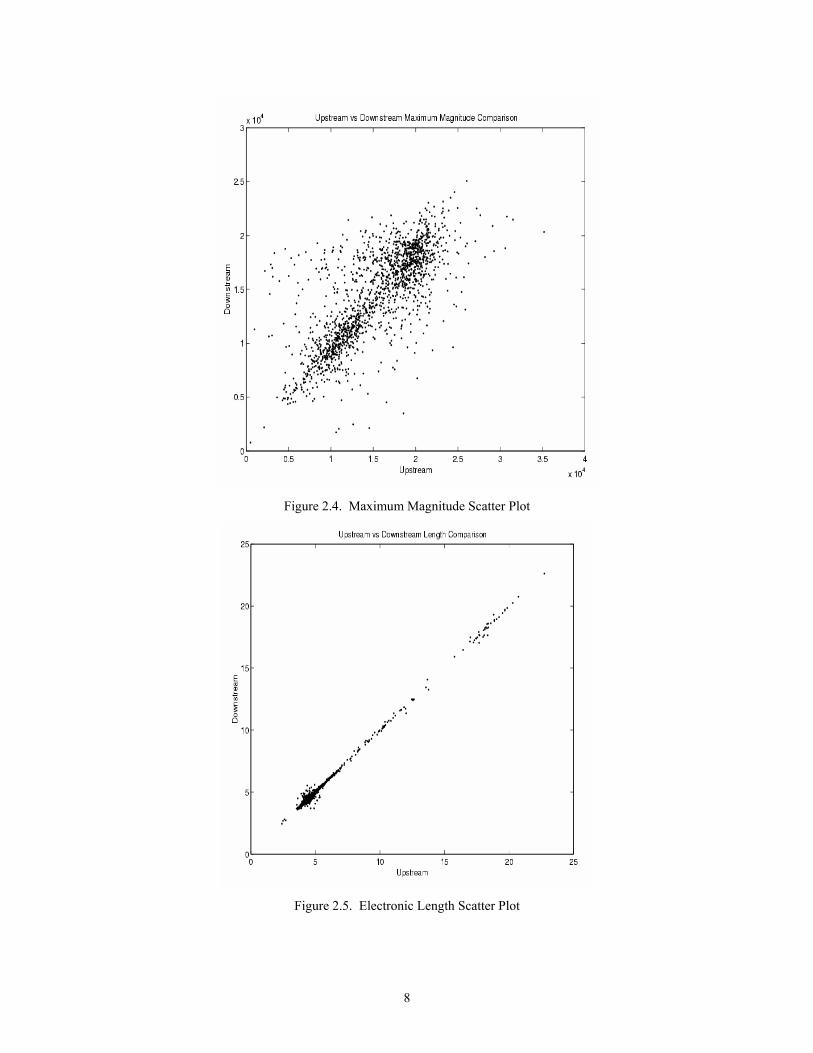
Figure 2.4. Maximum Magnitude Scatter Plot

Figure 2.5. Electronic Length Scatter Plot

8

Figure 2.6. SP Scatter Plot

Figure 2.7. DOS Scatter Plot

9

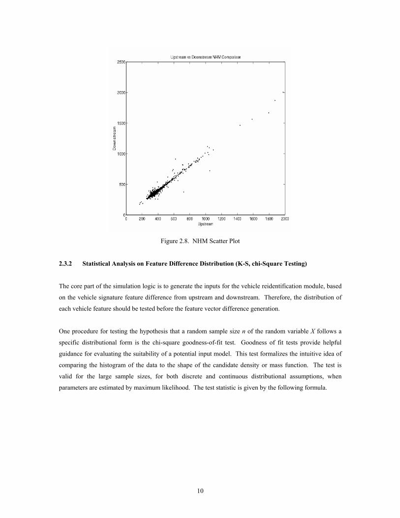
Figure 2.8. NHM Scatter Plot

2.3.2 Statistical Analysis on Feature Difference Distribution (K-S, chi-Square Testing)

The core part of the simulation logic is to generate the inputs for the vehicle reidentification module, based

on the vehicle signature feature difference from upstream and downstream. Therefore, the distribution of

each vehicle feature should be tested before the feature vector difference generation.

One procedure for testing the hypothesis that a random sample size n of the random variable X follows a

specific distributional form is the chi-square goodness-of-fit test. Goodness of fit tests provide helpful

guidance for evaluating the suitability of a potential input model. This test formalizes the intuitive idea of

comparing the histogram of the data to the shape of the candidate density or mass function. The test is

valid for the large sample sizes, for both discrete and continuous distributional assumptions, when

parameters are estimated by maximum likelihood. The test statistic is given by the following formula.

10

( )

intervalclassanalysis:

sizesample,obsevation:

intervalclassththewithassociatedyprobabilitedhypothesizl,Theoretica:

intervalclassththeinfrequencyExpected:

intervalclassththeinfrequencyObserved:

StatisticsSquareChi:

2

0

1

22

0

knpEO

pnEE

EO

i

i

i

where

i

i

i

ii

k

i i

ii

−

=

= ∑−

=

χ

χ

It can be shown that approximately follows the chi-square distribution with k-s-1 degree of freedom,

where s represents the number of parameters of the hypothesized distribution estimated by the sample

statistics. The hypotheses are :

χ 2

0

H0 : the random variable, X, conforms to the distributional assumption

H1 : the random variable, X, does not conform

The null hypothesis, H0, is rejected if > χ 2

0 χα

2

1, −−sk

In this study, in order to test the normal distribution, two parameters, mean and variance, should be

investigated with a degree of freedom of k-2-1, where k represents the analysis interval. Table 2.3 shows

the chi-square statistics and the results for five feature vectors. As presented in the Table, each feature

vector difference distribution cannot reject the null hypothesis at the five percent at level of significance,

and therefore, can be regarded as a normal distribution.

Table 2.3. Chi-Square Test (* ) 1.112

5,05.0=χ

Feature Vector Chi-Square Statistics (Hypothesis Testing)

Maximum Magnitude 9.33 (Cannot reject the H0)

Length 9.91 (Cannot reject the H0)

Shape Parameter (SP) 10.98 (Cannot reject the H0)

Number of High Magnitude (NHM) 8.45 (Cannot reject the H0)

Degree of Symmetry (DOS) 3.62 (Cannot reject the H0)

11

2.3.3 Vehicle Clustering

Efforts to find out the error distribution discussed above were performed with actual vehicle signatures.

Basically, a unique vehicle signature is observed from each individual vehicle. However, it is impractical to

estimate each single error distribution for each individual vehicle. A clustering technique was employed to

overcome this limitation based on the assumption that vehicles in the same cluster would generate similar

vehicle signatures and the generated signatures would be distinct from those of other vehicles in different

clusters.

The vehicle signatures in the dataset were clustered based on their similarities. This clustering should meet

two requirements: homogeneity of vehicle signatures within the same categories, i.e. data that belong to the

same category should be as similar as possible, and heterogeneity of vehicle signatures between categories,

i.e. data belonging to different categories should be as different as possible. For clustering analysis, the

feature differences extracted from individual vehicles passing between upstream and downstream detectors

were used. The number of clusters corresponds to the number of vehicle types specified in PARAMICS.

However, the number of clusters to use is an issue because it can affect the performance of the vehicle

reidentification algorithm. To determine a reasonable number of vehicle clusters, we selected a number of

clusters that was able to reproduce the actual performance of vehicle reidentification, which we have

obtained from the field. So far, the vehicle reidentification performance in the freeway has attained about

70 ~ 80% of correct matching rate based on the previous studies (Sun et al, 1999; TO 4122).

12

CHAPTER 3 REIDENTIFICATION SYSTEM DEVELOPMENT

3.1 Introduction

The fundamental idea of vehicle reidentification based on inductive signatures is to match a given

downstream vehicle signature with an upstream vehicle signature from amongst a set of candidate upstream

vehicle signatures. Applying the concept of the lexicographic method developed by Sun et al. (1999) for

freeway applications, vehicle reidentification was formulated as a five-level optimization problem.

Minimizing mismatches between feature vector pairs denotes the “optimization” on any given objective.

Vehicle reidentification is the pattern recognition procedure based on a set of vehicles. For each detected

vehicle at downstream, the system tries to capture possible matching vehicles from the corresponding

upstream station. To reach higher performance rate in vehicle matching, the search for optimal upstream

candidate set for each downstream vehicle is critical. This selecting procedure is called optimal candidate

searching and several levels of restriction are applied to obtain the final optimal candidate set. Figure 3.1

shows multi - level restriction for the vehicle reidentification system. The restriction can be divided into

two categories. Vehicle specific feature restriction and traffic specific restriction. In vehicle specific

feature restriction, the elimination of most unlikely identical upstream vehicles is processed based on the

vehicle’s physical attributes. Traffic specific feature restriction includes the possible upstream set

searching as well as time window setting. The first step of this restriction is to reduce the spatial search

space, which identifies the upstream origin of each vehicle. The next step of the search space restriction is

temporal search space reduction, which establishes a lower and upper bound for feasible travel time, called

a ‘time window’. For both freeways and arterials, this procedure is more complicated than vehicle specific

feature restriction because it involves time/flow variant traffic dynamics. In arterial case, because of the

signal interruption, this step is more challenging part. The following sections will discuss the

complications and resolution points.

13

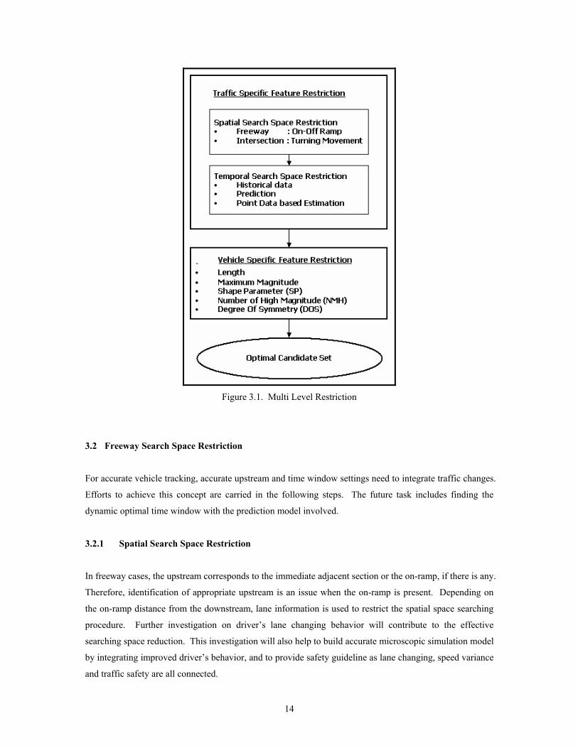
Figure 3.1. Multi Level Restriction

3.2 Freeway Search Space Restriction

For accurate vehicle tracking, accurate upstream and time window settings need to integrate traffic changes.

Efforts to achieve this concept are carried in the following steps. The future task includes finding the

dynamic optimal time window with the prediction model involved.

3.2.1 Spatial Search Space Restriction

In freeway cases, the upstream corresponds to the immediate adjacent section or the on-ramp, if there is any.

Therefore, identification of appropriate upstream is an issue when the on-ramp is present. Depending on

the on-ramp distance from the downstream, lane information is used to restrict the spatial space searching

procedure. Further investigation on driver’s lane changing behavior will contribute to the effective

searching space reduction. This investigation will also help to build accurate microscopic simulation model

by integrating improved driver’s behavior, and to provide safety guideline as lane changing, speed variance

and traffic safety are all connected.

14

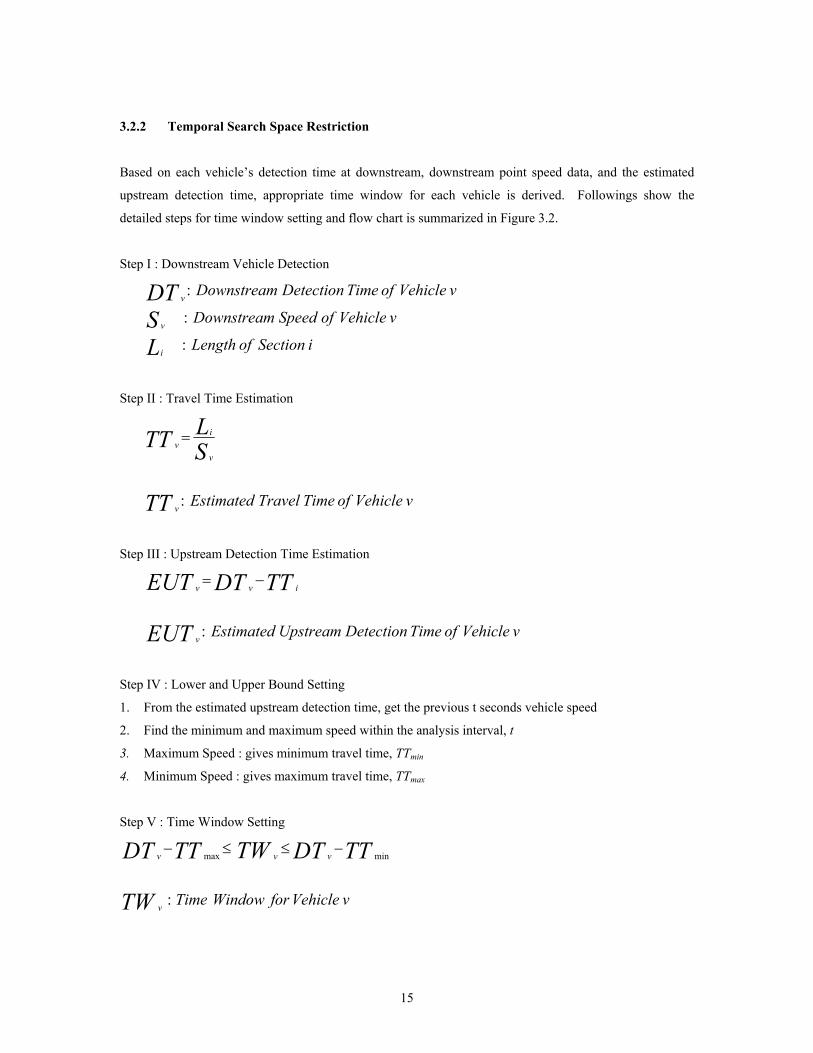
3.2.2 Temporal Search Space Restriction

Based on each vehicle’s detection time at downstream, downstream point speed data, and the estimated

upstream detection time, appropriate time window for each vehicle is derived. Followings show the

detailed steps for time window setting and flow chart is summarized in Figure 3.2.

Step I : Downstream Vehicle Detection

iSectionofLength

vVehicleofSpeedDownstream

vVehicleofTimeDetectionDownstream

LSDT

i

v

v

:

:

:

Step II : Travel Time Estimation

vVehicleofTimeTravelEstimatedTT

SLTT

v

v

iv

:

=

Step III : Upstream Detection Time Estimation

vVehicleofTimeDetectionUpstreamEstimatedEUT

TTDTEUT

v

ivv

:

−=

Step IV : Lower and Upper Bound Setting

1. From the estimated upstream detection time, get the previous t seconds vehicle speed

2. Find the minimum and maximum speed within the analysis interval, t

3. Maximum Speed : gives minimum travel time, TTmin

4. Minimum Speed : gives maximum travel time, TTmax

Step V : Time Window Setting

vVehicleforWindowTimeTW

TTDTTWTTDT

v

vvv

:

minmax −≤≤−

15

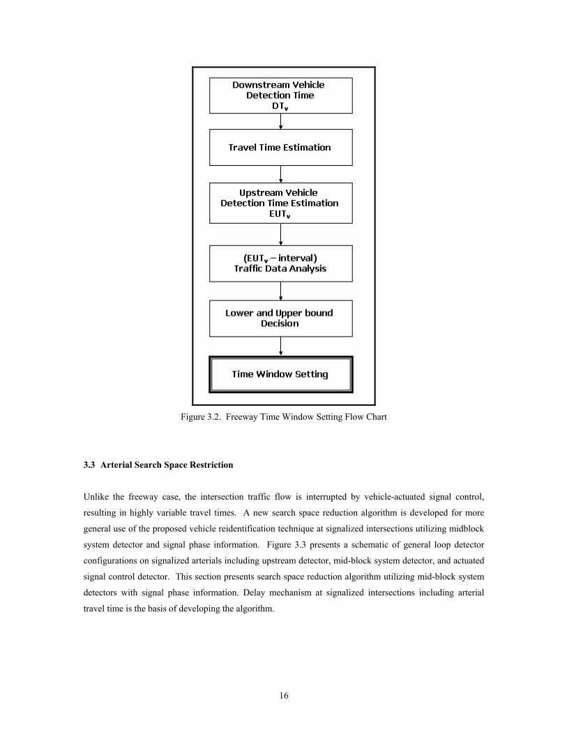
Figure 3.2. Freeway Time Window Setting Flow Chart

3.3 Arterial Search Space Restriction

Unlike the freeway case, the intersection traffic flow is interrupted by vehicle-actuated signal control,

resulting in highly variable travel times. A new search space reduction algorithm is developed for more

general use of the proposed vehicle reidentification technique at signalized intersections utilizing midblock

system detector and signal phase information. Figure 3.3 presents a schematic of general loop detector

configurations on signalized arterials including upstream detector, mid-block system detector, and actuated

signal control detector. This section presents search space reduction algorithm utilizing mid-block system

detectors with signal phase information. Delay mechanism at signalized intersections including arterial

travel time is the basis of developing the algorithm.

16

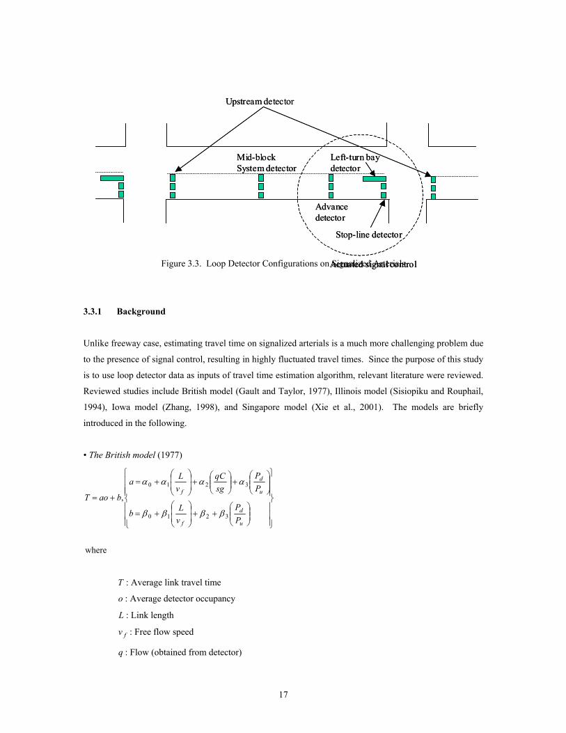
Figure 3.3. Loop Detector Configurations on Signalized Arterials AA

Upstream detector

Mid-blockSystem detector

Advance detector

Left-turn bay detector

Stop-line detector

ctuated signal control

Upstream detector

Mid-blockSystem detector

Advance detector

Left-turn bay detector

Stop-line detector

ctuated signal control

3.3.1 Background

Unlike freeway case, estimating travel time on signalized arterials is a much more challenging problem due

to the presence of signal control, resulting in highly fluctuated travel times. Since the purpose of this study

is to use loop detector data as inputs of travel time estimation algorithm, relevant literature were reviewed.

Reviewed studies include British model (Gault and Taylor, 1977), Illinois model (Sisiopiku and Rouphail,

1994), Iowa model (Zhang, 1998), and Singapore model (Xie et al., 2001). The models are briefly

introduced in the following.

• The British model (1977)

where

,

3210

3210

++

+=

+

+

+=

+=

u

d

f

u

d

f

PP

vLb

PP

sgqC

vLa

baoT

ββββ

αααα

T : Average link travel time

o : Average detector occupancy

L : Link length

fv : Free flow speed

q : Flow (obtained from detector)

17

C : Cycle length

g : Green time

dP : Downstream green time

uP : Upstream green time

βα , : Regression coefficient

• The Illinois model (1994)

where

det 4321 grnratboblocbbvLTf

++++=

: Ratio of detector setback from the stopline over link length locdet

grnrat : Effective green ratio ( ) Cg /

: Regression coefficient b

• The Iowa model (1999)

( )

where

379.0

exp,)1(

/

'/

//

=

−=−+=

oqu

Xuuuuu

oq

fcv

oqcv

βαγγ

calibrated be toparameter Model :,,

1)(0 factor, Weight :

max ratio V/C Critical :

speedJourney :

,...,1

βα

γγ

f

ii

ini

u

gsCq

X

u

≤≤

=

=

• The Singapore model (2001)

18

( )( ) ( )

where

121219.0

22

det

−+

−−

+=xq

xx

Cu

LTλλφ

: Maximum speed of the downstream and upstream detector stations detu

φ : Downstream queue factor (more details of φ can be found in the literature)

It has been identified that proposed models in the literature are based on statistical modeling using

regression analysis. Travel time model for signalized arterials can be viewed as the combination of running

time and signal delay. The major factors affecting running time are free flow speed and link length defined

by upstream and downstream detector stations. On the other hand, signal delay is a function of signal

control parameters such as cycle length and green time. Of course, traffic volume provides a significant

impact on both running time and signal delay. This study develops an arterial travel time model that will

be used for establishing time window based on these findings.

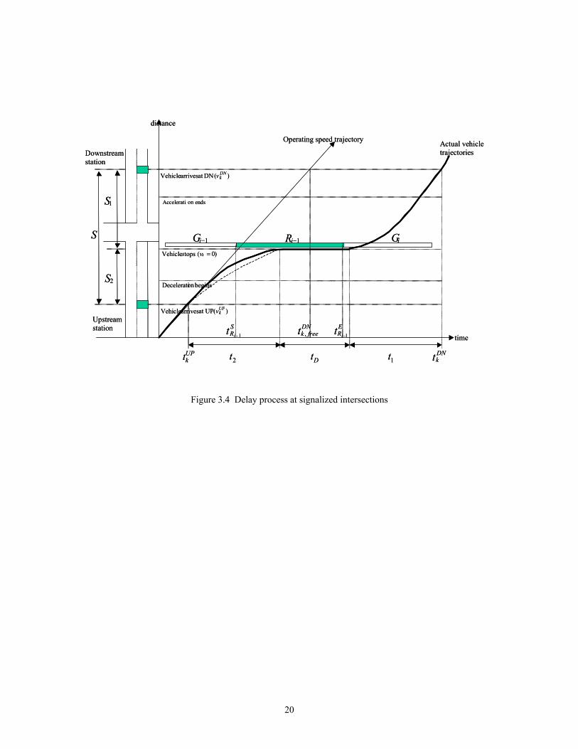
Estimating travel time is a basis for establishing time window, which reduces upstream candidate vehicles.

Travel time between detection stations for vehicle reidentification at signalized intersections consists of

three components. These components include stopped delay ( ), time spent from upstream detector

location to the end of the queue ( ), and time spent from stopline to downstream detector location ( ) as

shown in Figure 3.4. Minimum and maximum travel times of vehicle k are derived from the delay process

at signalized intersections, and further utilized for time window.

Dt

2t 1t

19

Operating speed trajectory

Upstream station

Downstream station

distance

time

Actual vehicle trajectories

) ( DN at arrives Vehicle DN k v

) ( at UP arrives Vehicle UP k v

) 0 ( tops Vehicle = k v s

ends on Accelerati

begins on Decelerati

DN k t 1tDt2t UP

k t

SRit 1−

ERit 1−

1−iR1 − i G iG

DNfreekt ,

1 S

2 S

S

Operating speed trajectory

Upstream station

Downstream station

distance

time

Actual vehicle trajectories

) ( DN at arrives Vehicle DN k v

) ( at UP arrives Vehicle UP k v

) 0 ( tops Vehicle = k v s

ends on Accelerati

begins on Decelerati

DN k t 1tDt2t UP

k t

SRit 1−

ERit 1−

1−iR1 − i G iG

DNfreekt ,

1 S

2 S

S

Figure 3.4 Delay process at signalized intersections

20

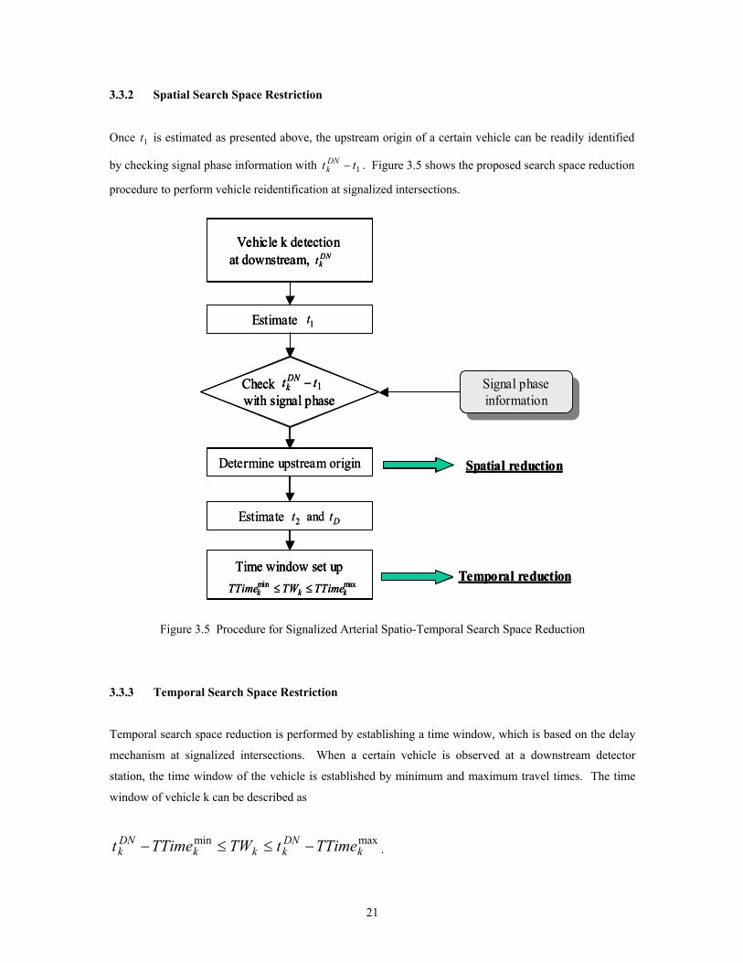
3.3.2 Spatial Search Space Restriction

Once is estimated as presented above, the upstream origin of a certain vehicle can be readily identified

by checking signal phase information with t . Figure 3.5 shows the proposed search space reduction

procedure to perform vehicle reidentification at signalized intersections.

1t

1tDNk −

Vehicle k detection at downstream, DN

kt

Determine upstream origin

Estimate Dtt and 2

Time window set upmaxminkkk TTimeTWTTime ≤≤

Spatial reduction

Temporal reduction

Estimate 1t

Check with signal phase

tt DNk − 1 Signal phase

information

Signal phaseinformation

Vehicle k detection at downstream, DN

ktVehicle k detection

at downstream, DNkt

Determine upstream origin

Estimate Dtt and 2

Time window set upmaxminkkk TTimeTWTTime ≤≤

Time window set upmaxminkkk TTimeTWTTime ≤≤

Spatial reduction

Temporal reduction

Estimate 1t

Check with signal phase

tt DNk − 1Check

with signal phasett DN

k − 1 Signal phaseinformation

Signal phaseinformation

Figure 3.5 Procedure for Signalized Arterial Spatio-Temporal Search Space Reduction

3.3.3 Temporal Search Space Restriction

Temporal search space reduction is performed by establishing a time window, which is based on the delay

mechanism at signalized intersections. When a certain vehicle is observed at a downstream detector

station, the time window of the vehicle is established by minimum and maximum travel times. The time

window of vehicle k can be described as

maxmink

DNkkk

DNk TTimetTWTTimet −≤≤− .

21

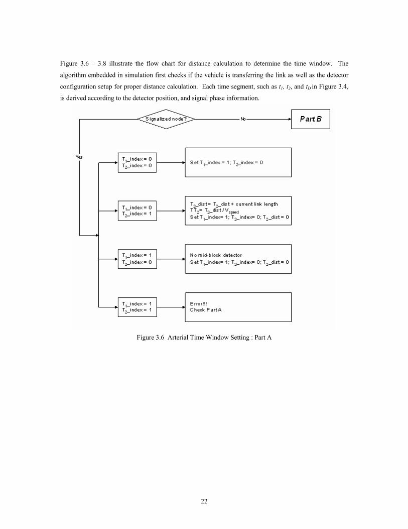
Figure 3.6 – 3.8 illustrate the flow chart for distance calculation to determine the time window. The

algorithm embedded in simulation first checks if the vehicle is transferring the link as well as the detector

configuration setup for proper distance calculation. Each time segment, such as t1, t2, and tD in Figure 3.4,

is derived according to the detector position, and signal phase information.

Figure 3.6 Arterial Time Window Setting : Part A

22

Figure 3.7 Arterial Time Window Setting : Part B

Figure 3.8 Arterial Time Window Setting : Part C

23

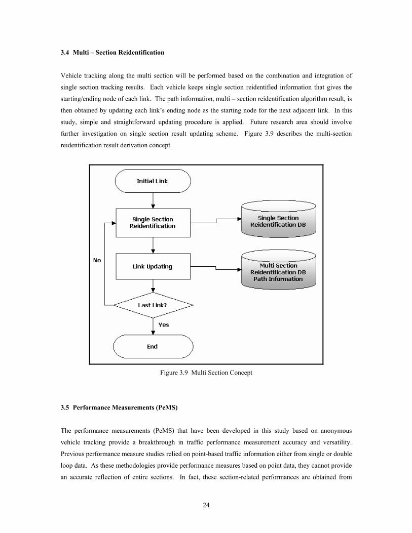
3.4 Multi – Section Reidentification

Vehicle tracking along the multi section will be performed based on the combination and integration of

single section tracking results. Each vehicle keeps single section reidentified information that gives the

starting/ending node of each link. The path information, multi – section reidentification algorithm result, is

then obtained by updating each link’s ending node as the starting node for the next adjacent link. In this

study, simple and straightforward updating procedure is applied. Future research area should involve

further investigation on single section result updating scheme. Figure 3.9 describes the multi-section

reidentification result derivation concept.

Figure 3.9 Multi Section Concept

3.5 Performance Measurements (PeMS)

The performance measurements (PeMS) that have been developed in this study based on anonymous

vehicle tracking provide a breakthrough in traffic performance measurement accuracy and versatility.

Previous performance measure studies relied on point-based traffic information either from single or double

loop data. As these methodologies provide performance measures based on point data, they cannot provide

an accurate reflection of entire sections. In fact, these section-related performances are obtained from

24

extrapolations from a single point in the network. Since traffic movement represents a dynamic

compressible flow, it is not possible to assume uniform conditions across an entire section based on

measurements from a single point. While point measurements may be accurate at the immediate vicinity of

the detector station, they would provide erroneous estimates for street or freeway sections, which typically

span between one and three quarters of a mile.

With the critical need for a comprehensive performance measurement system and the limitations of the

present systems, it is imperative to develop new performance measures that are able to provide traffic

information representative of piecewise continuous road sections. Through the implementation of the

anonymous vehicle tracking system, vehicles can be tracked across freeway sections, street sections and

even street intersections. Hence, accurate section travel times and speeds can be obtained without

compromising the privacy of vehicle occupants. Besides, this system can be readily expanded to track

vehicles across multiple sections to obtain performance measures of not just individual road segments, but

origin-destination paths in extensive road networks. The following table summarizes the performance

measurement details that can be obtained at information and network levels and data applications.

25

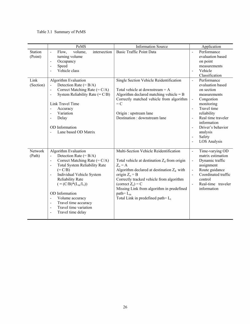
Table 3.1 Summary of PeMS

PeMS Information Source Application Station (Point)

- Flow, volume, intersection turning volume

- Occupancy - Speed - Vehicle class

Basic Traffic Point Data - Performance evaluation based on point measurements

- Vehicle Classification

Link (Section)

Algorithm Evaluation - Detection Rate (= B/A) - Correct Matching Rate (= C/A) - System Reliability Rate (= C/B) Link Travel Time - Accuracy - Variation - Delay OD Information - Lane based OD Matrix

Single Section Vehicle Reidentification Total vehicle at downstream = A Algorithm declared matching vehicle = B Correctly matched vehicle from algorithm = C Origin : upstream lane Destination : downstream lane

- Performance evaluation based on section measurements

- Congestion monitoring

- Travel time reliability

- Real time traveler information

- Driver’s behavior analysis

- Safety - LOS Analysis

Network (Path)

Algorithm Evaluation - Detection Rate (= B/A) - Correct Matching Rate (= C/A) - Total System Reliability Rate (= C/B) - Individual Vehicle System

Reliability Rate ( = (C/B)*(Lm/Lt)) OD Information - Volume accuracy - Travel time accuracy - Travel time variation - Travel time delay

Multi-Section Vehicle Reidentification Total vehicle at destination Zd from origin Zo = A Algorithm declared at destination Zd with origin Zo = B Correctly tracked vehicle from algorithm (correct Zo) = C Missing Link from algorithm in predefined path= Lm Total Link in predefined path= Lt

- Time-varying OD matrix estimation

- Dynamic traffic assignment

- Route guidance - Coordinated traffic

control - Real-time traveler

information

26

CHAPTER 4 SIMULATION FRAMEWORK

4.1 Introduction

The proposed evaluation framework employs PARAMICS microscopic traffic simulator. To date, various

simulation models have been used for evaluating ATMIS strategies. Traffic simulation models can be

broadly classified into two groups: microscopic and macroscopic models. As recently developed ATMIS

strategies often require the observation of very detailed levels of traffic phenomenon such as individual

vehicle movements, the microscopic simulation model is better suited for such needs, although model

validation and calibration issues still need to be solved. Many studies have used microscopic simulation

models for evaluating dynamic traffic assignment, route guidance, signal control, incident detection, and

ramp control strategies. However, the traffic surveillance system, which is a core part of such strategies,

has not been evaluated under the simulation environment. One of the invaluable features of this study is to

present a methodology on how to use microscopic simulation models for evaluating traffic surveillance

system. The proposed simulation framework could be of great value for testing and performance

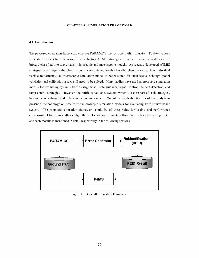
comparison of traffic surveillance algorithms. The overall simulation flow chart is described in Figure 4.1

and each module is mentioned in detail respectively in the following sections.

Figure 4.1. Overall Simulation Framework

27

4.2 PARAMICS

PARAMICS (PARAllel MICroscopic Simulation) is a parallel, microscopic, scalable, user programmable

and computationally efficient traffic simulation model (Duncan, 1995; Quadstone Ltd., 2003) that has been

used for many applications in the ATMS Testbed. Individual vehicles are modeled in fine detail for the

duration of their entire trip, providing comprehensive traffic characteristics and congestion information, as

well as enabling the modeling of the interface between drivers and Intelligent Transportation Systems

facilities and strategies.

The Testbed network (for Orange County) coded into PARAMICS consists of 5,400 nodes, 12,160 links

and 420 zones, and provides a highly detailed 3-dimensionally and geographically correct representation

for traffic and ITS simulations. This network is coded for over 200,000 vehicle trips across both freeways

and major arterials in the 4-6pm afternoon peak period. This network is also calibrated based on UCI

Testbed archived real world dataset. At ITS-Irvine, PARAMICS currently operates on an SGI Origin2000

mutiprocessor workstation. With this system, over 90,000 vehicles can be simulated in real-time (or fewer

vehicles in faster than real-time) (Lee, 1998).

A notable feature of PARAMICS is its scalability. A large network, such as that for the California ATMS

Testbed, can be decomposed into regions where each is simulated on a processor in a parallel machine.

This scalability enables development to start off small and then grow, and provides the potential for

achieving faster than real-time, multi-scenario simulations. Another major feature of PARAMICS is its

Application Programming Interface (API). The API allows the user to customize many features of the

underlying simulation model, and to link PARAMICS to other applications developed by the user.

Moreover the API allows additional functionality by adding more external modeling routines. Additional

PARAMICS key features include:

• A fully integrated and interactive graphical network editor and manager

• A highly detailed definitions of roadway network, travel demand, driver, vehicle, and traffic control

devices

• ITS-capability, featuring integrated simulation of ITS components, including a variety of traffic

management, information and control strategies

• Capability of modeling pre-timed and actuated signal control mechanisms

• Capability of modeling vehicle emissions, incident, bus, and car parking

• A fully integrated visualization tools to display simulation results

28

4.3 Network Setting and Tracking Module

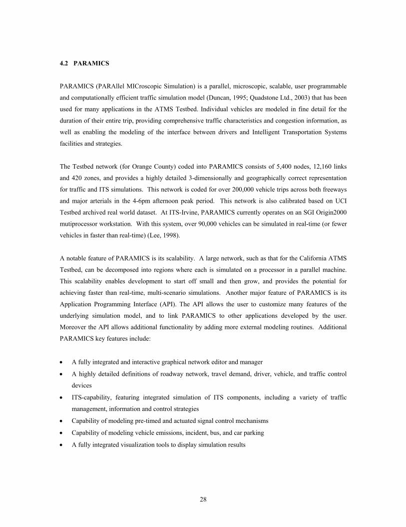
The initial step to build the simulation framework is discussed in this section. Parameters setting, network

scope decision and API module implementation for vehicle tracking are the major tasks. The inter-relation

among those factors is illustrated in Figure 4.2.

A central control module in PARAMICS is connected with both arterial and freeway vehicle tracking API

module. Detector ID information will contribute to identify the network attribute to set the corresponding

reidentification algorithm. In PARAMICS, users are able to define not only vehicle types but also the

proportions of such vehicle types in traffic streams. In addition, the physical characteristics of each vehicle

including length, height, width, maximum speed, acceleration and deceleration can also be specified.

Based on the analysis of vehicle signatures discussed in the previous chapter, we pre-defined vehicle types

and vehicle proportions in PARAMICS prior to running the simulation. The calibrated parameters, such as

reaction time and headway, were set according to the previous studies (Chu et al 2003, 2004).

Figure 4.2 PARAMICS Modeller

The network site for the proposed study covers the I-405 corridor and 36 arterial intersections in southern

California. The entire study site network is presented in Figure 4.3.

In freeway setting, I-405 and SR-133 were the major freeway corridors with five consecutive interchanges.

The interested five interchanges are:

1. I-405 and Jeffrey

2. I-405 and Sand Canyon

29

3. I-405 and SR-133

4. I-405 and Irvine Center Dr.

5. SR-133 and Barranca

A total 115 detector stations were coded including on-ramp detectors, off- ramp detectors, and mainline

detectors. The freeway was configured with six lanes and a speed limit of 65 mph, while on-ramps had a

speed limit of 40 mph. A total of five zones were connected with the freeway traffic demand.

Figure 4.3 Proposed Study Site

In the arterial network, 36 intersections in city of Irvine were included. They were coded with a three -

lane configuration and a speed limit of 40 mph. A total of 156 detection stations and 30 zones were

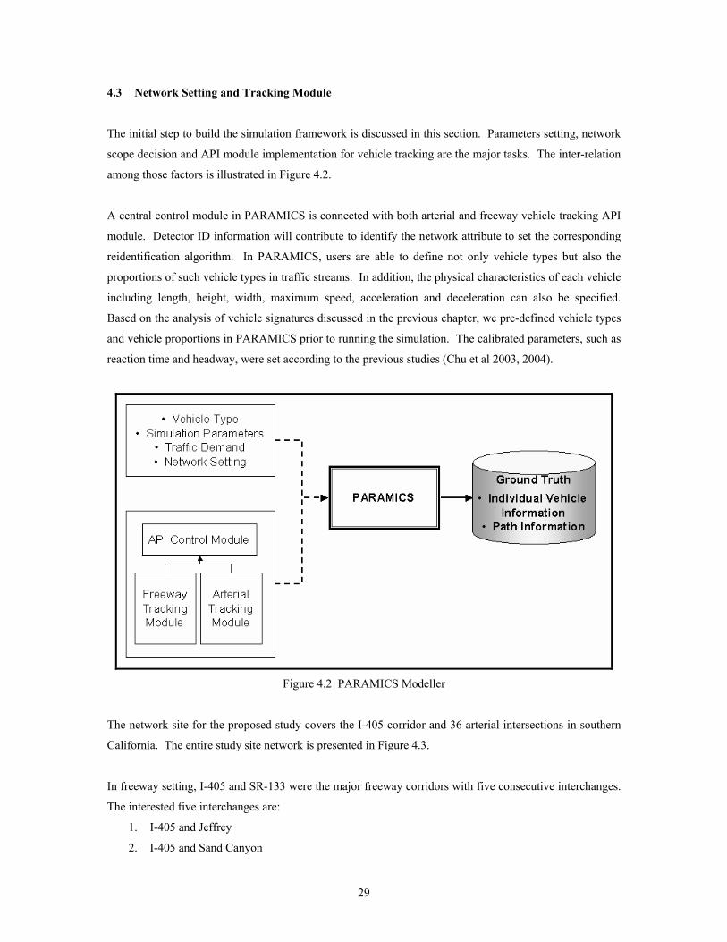
implemented. Table 4.1 lists the 36 intersections coded in the simulation network.

30

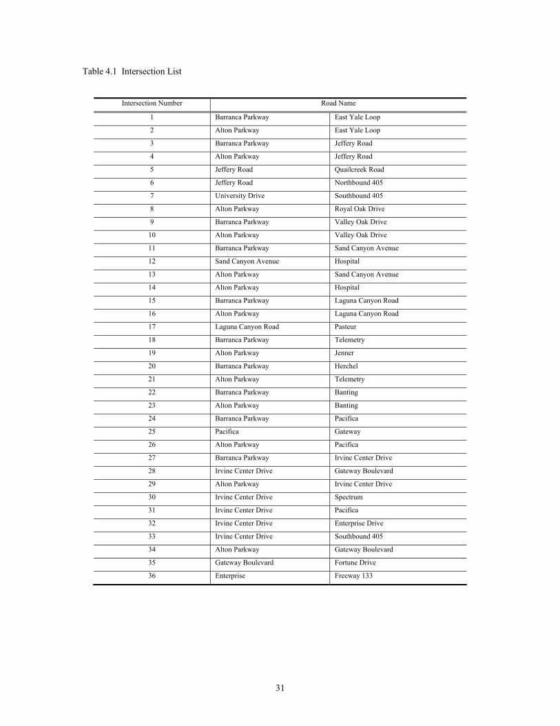
Table 4.1 Intersection List

Intersection Number Road Name

1 Barranca Parkway East Yale Loop

2 Alton Parkway East Yale Loop

3 Barranca Parkway Jeffery Road

4 Alton Parkway Jeffery Road

5 Jeffery Road Quailcreek Road

6 Jeffery Road Northbound 405

7 University Drive Southbound 405

8 Alton Parkway Royal Oak Drive

9 Barranca Parkway Valley Oak Drive

10 Alton Parkway Valley Oak Drive

11 Barranca Parkway Sand Canyon Avenue

12 Sand Canyon Avenue Hospital

13 Alton Parkway Sand Canyon Avenue

14 Alton Parkway Hospital

15 Barranca Parkway Laguna Canyon Road

16 Alton Parkway Laguna Canyon Road

17 Laguna Canyon Road Pasteur

18 Barranca Parkway Telemetry

19 Alton Parkway Jenner

20 Barranca Parkway Herchel

21 Alton Parkway Telemetry

22 Barranca Parkway Banting

23 Alton Parkway Banting

24 Barranca Parkway Pacifica

25 Pacifica Gateway

26 Alton Parkway Pacifica

27 Barranca Parkway Irvine Center Drive

28 Irvine Center Drive Gateway Boulevard

29 Alton Parkway Irvine Center Drive

30 Irvine Center Drive Spectrum

31 Irvine Center Drive Pacifica

32 Irvine Center Drive Enterprise Drive

33 Irvine Center Drive Southbound 405

34 Alton Parkway Gateway Boulevard

35 Gateway Boulevard Fortune Drive

36 Enterprise Freeway 133

31

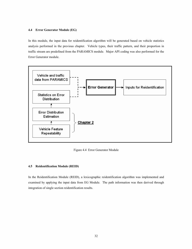
4.4 Error Generator Module (EG)

In this module, the input data for reidentification algorithm will be generated based on vehicle statistics

analysis performed in the previous chapter. Vehicle types, their traffic pattern, and their proportion in

traffic stream are predefined from the PARAMICS module. Major API coding was also performed for the

Error Generator module.

Figure 4.4 Error Generator Module

4.5 Reidentification Module (REID)

In the Reidentification Module (REID), a lexicographic reidentification algorithm was implemented and

examined by applying the input data from EG Module. The path information was then derived through

integration of single section reidentification results.

32

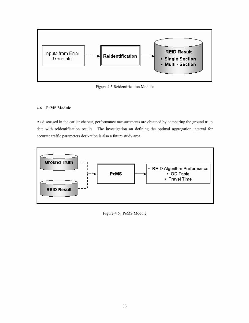
Figure 4.5 Reidentification Module

4.6 PeMS Module

As discussed in the earlier chapter, performance measurements are obtained by comparing the ground truth

data with reidentification results. The investigation on defining the optimal aggregation interval for

accurate traffic parameters derivation is also a future study area.

Figure 4.6. PeMS Module

33

CHAPTER 5 PARAMICS EXPERIMENTAL DESIGN AND RESULT ANALYSIS

5.1 Introduction

Invaluable section-related traffic information can be obtained by tracking individual vehicles. In this

section, travel time is chosen as the main analysis component since it is one of the most important traffic

measurement parameters for successful and efficient traffic operations and control. The search for an

optimal aggregation interval was conducted based on the assessment of travel time percentage error. In this

section, five different aggregation intervals were used. Furthermore, three types of path, with different road

geometry compositions, were also selected for expanded research scope. The following subsections will

explain each analysis step in detail.

5.2 PARAMICS Setting

Traffic demand was set to be moderate flow throughout the simulation running. The simulation duration,

which consisted of a total of 45-minute simulation running time, with 20-minute warmup time, was

deployed due to limitations of computer processors. The warmup time served to ascertain stable traffic

flow conditions before executing the vehicle re-identification algorithm. The vehicle-releasing pattern

followed the normal distribution and a total of 30 simulation runs with different seed numbers were

performed. In average, there were 4470 vehicles that were released after the warm-up time period and

therefore, were subject to the REID API running. Among those 4470 vehicles, about 1500 vehicles were

declared as reidentified by the implemented REID API. Details on REID module results will be mentioned

in the following section.

In this study, three different paths that varied with road type were selected for further analysis. Path 1 was

mainly composed of I-405 freeway sections. Arterial links were the main components for path 2. In path 3,

freeway and arterial sections were mixed. With this setup, the effect of vehicle re-identification results on

estimated travel time accuracy at different locations and paths can also be examined. Figure 5.1 explains

the overall study site as well as three different paths.

34

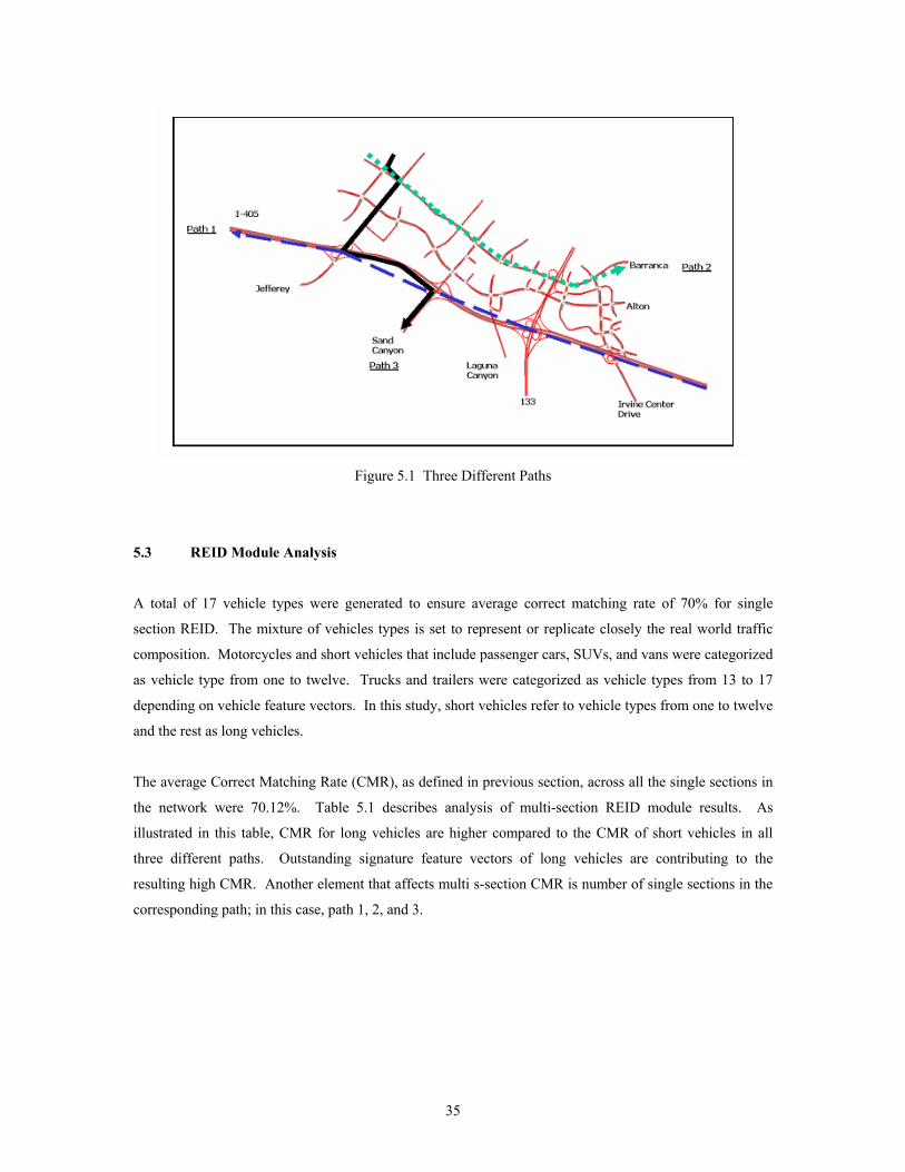
Figure 5.1 Three Different Paths

5.3 REID Module Analysis

A total of 17 vehicle types were generated to ensure average correct matching rate of 70% for single

section REID. The mixture of vehicles types is set to represent or replicate closely the real world traffic

composition. Motorcycles and short vehicles that include passenger cars, SUVs, and vans were categorized

as vehicle type from one to twelve. Trucks and trailers were categorized as vehicle types from 13 to 17

depending on vehicle feature vectors. In this study, short vehicles refer to vehicle types from one to twelve

and the rest as long vehicles.

The average Correct Matching Rate (CMR), as defined in previous section, across all the single sections in

the network were 70.12%. Table 5.1 describes analysis of multi-section REID module results. As

illustrated in this table, CMR for long vehicles are higher compared to the CMR of short vehicles in all

three different paths. Outstanding signature feature vectors of long vehicles are contributing to the

resulting high CMR. Another element that affects multi s-section CMR is number of single sections in the

corresponding path; in this case, path 1, 2, and 3.

35

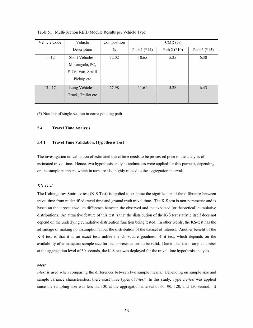
Table 5.1 Multi-Section REID Module Results per Vehicle Type

CMR (%) Vehicle Code Vehicle

Description

Composition

% Path 1 (*14) Path 2 (*10) Path 3 (*15)

1 - 12 Short Vehicles -

Motorcycle, PC,

SUV, Van, Small

Pickup etc

72.02 10.65 5.25 6.30

13 - 17 Long Vehicles -

Truck, Trailer etc

27.98 11.61 5.28 6.43

(*) Number of single section in corresponding path

5.4 Travel Time Analysis

5.4.1 Travel Time Validation, Hypothesis Test

The investigation on validation of estimated travel time needs to be processed prior to the analysis of

estimated travel time. Hence, two hypothesis analysis techniques were applied for this purpose, depending

on the sample numbers, which in turn are also highly related to the aggregation interval.

KS Test The Kolmogorov-Smirnov test (K-S Test) is applied to examine the significance of the difference between

travel time from reidentified travel time and ground truth travel time. The K-S test is non-parametric and is

based on the largest absolute difference between the observed and the expected (or theoretical) cumulative

distributions. An attractive feature of this test is that the distribution of the K-S test statistic itself does not

depend on the underlying cumulative distribution function being tested. In other words, the KS-test has the

advantage of making no assumption about the distribution of the dataset of interest. Another benefit of the

K-S test is that it is an exact test, unlike the chi-square goodness-of-fit test, which depends on the

availability of an adequate sample size for the approximations to be valid. Due to the small sample number

at the aggregation level of 30 seconds, the K-S test was deployed for the travel time hypothesis analysis.

t-test

t-test is used when comparing the differences between two sample means. Depending on sample size and

sample variance characteristics, there exist three types of t-test. In this study, Type 2 t-test was applied

since the sampling size was less than 30 at the aggregation interval of 60, 90, 120, and 150-second. It

36

should be noted that the vehicle- releasing pattern follows the normal distribution and therefore samples

satisfy one of the requirement of a Type 2 t-test.

Table 5.2 shows the two hypotheses test procedure mentioned in this study.

Results

Both KS test and t-test results show that the estimated travel time does conform to the true travel time for

all paths and at all aggregation intervals. The results demonstrate that the re-identification system is

capable of producing accurate estimates of travel time information

37

Table 5.2 Hypothesis Procedure

Step I : Hypothesis Definition

H0 : Reidentified travel time distribution conforms to the real travel time distribution

H1 : Reidentified travel time distribution does not conform to the real travel time distribution

Or : , : 0H 21−−

= XX 1H 21−−

≠ XX

Step II : Level of significance Definition

α =0.05

Step III : Statistics Calculation

KS test

KS

= Max(difference value between theoretical

cumulative curve and sample cumulative curve)

t-test

)/1()/1()(

21

21

nnSXXT

p +−

=

−−

1n : Sample Size of Group 1

2n : Sample Size of Group 2

2)1()1(

21

222

2112

−+−+−

=nn

SnSnS p

(Pooling variance)

Step IV : Degree of Freedom Definition

KS test

1+−= ρν n

n : sample number

ρ : number of estimated parameter

t-test

221 −+= nnν

Step V : Decision Making – Rejection Area

KS test

αKSKS >

t-test

2

2

α

α

tT

tT

>

−< Two-tailed test.

38

5.4.2 Estimated Travel Time Analysis

The preceding analysis on travel time validation has shown that it was safe to conclude that the estimated

travel time represents the true travel time at all five different aggregation levels. Identifying the optimal

travel time aggregation intervals for generating useful traffic information accounting for the real-time

performance of transportation systems is an important issue in the field of traffic surveillance and

information systems. In this section, estimated travel time accuracy was assessed at five different

aggregation intervals.

Analysis Index

Total travel time percentage error (TotTTPE) was applied as the index for accuracy analysis and the

following formula shows the TotTTPE calculation procedure. At each step, the travel time accuracy is

evaluated based on the comparison between the system declared travel time and ground-truthed travel time.

TotTTPE is the average of these step-by-step percentage errors. Five different aggregation intervals are

applied in this study.

steptimeanalysis:intervalduringvolumetruthGround:

intervalduringvolumeREID:

intervalwithinvehicleindividualfortimetravelREID:

intervalwithinvehicleindividualfortimetraveltruthGround:

intervalaterrorpercentagetimeTravel:

100

1

11

kk

k

kj

ki

kwhere

N

RNN

abs

NRNRTTGTTTTPE

NGTT

RNRTT

NGTT

TTPE

k

k

kj

k

i

k

ki

k

i

kj

kj

ki

k

i

kk

kk

−

×=

∑

∑∑

=

==

39

intervalanalysistotalofnumber:

intervalaterrorpercentagetimeTravel:

errorpercentagetimetravelTotal:

100 1

INTTTPETotTTPE

INTTTPE

TotTTPE

k

where

k

INT

k

k

×=∑=

In addition to TotTTPE, the effect of aggregation interval on travel time accuracy was investigated by the

percentage error changing rate (PE_CR) index shown as follows.

kll

kl

where

TotTTPECRPE

TotTTPETotTTPETotTTPECRPE

l

k

l

l

lkk

l

≠

−×=

ofintervalaterrorpercentagetimetravelTotal:

secondtointervalfromerrorpercentageofrateChanging:

100

_

_

Travel Time Result Analysis

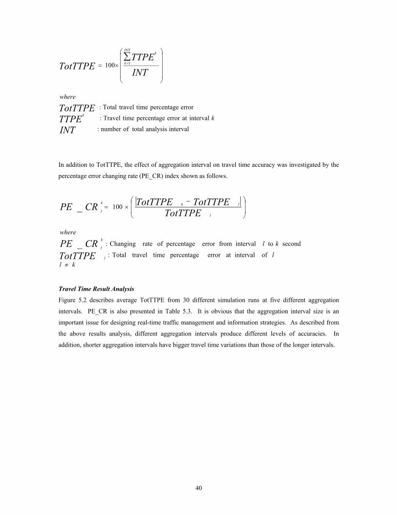
Figure 5.2 describes average TotTTPE from 30 different simulation runs at five different aggregation

intervals. PE_CR is also presented in Table 5.3. It is obvious that the aggregation interval size is an

important issue for designing real-time traffic management and information strategies. As described from

the above results analysis, different aggregation intervals produce different levels of accuracies. In

addition, shorter aggregation intervals have bigger travel time variations than those of the longer intervals.

40

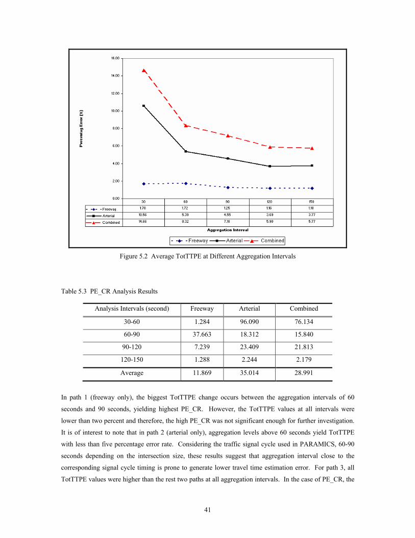
Figure 5.2 Average TotTTPE at Different Aggregation Intervals

Table 5.3 PE_CR Analysis Results

Analysis Intervals (second) Freeway Arterial Combined

30-60 1.284 96.090 76.134

60-90 37.663 18.312 15.840

90-120 7.239 23.409 21.813

120-150 1.288 2.244 2.179

Average 11.869 35.014 28.991

In path 1 (freeway only), the biggest TotTTPE change occurs between the aggregation intervals of 60

seconds and 90 seconds, yielding highest PE_CR. However, the TotTTPE values at all intervals were

lower than two percent and therefore, the high PE_CR was not significant enough for further investigation.

It is of interest to note that in path 2 (arterial only), aggregation levels above 60 seconds yield TotTTPE

with less than five percentage error rate. Considering the traffic signal cycle used in PARAMICS, 60-90

seconds depending on the intersection size, these results suggest that aggregation interval close to the

corresponding signal cycle timing is prone to generate lower travel time estimation error. For path 3, all

TotTTPE values were higher than the rest two paths at all aggregation intervals. In the case of PE_CR, the

41

highest value was observed between aggregation intervals of 30 and 60 seconds. Comparison between

estimated and true travel times at the 60-second aggregation interval is depicted in Figure 5.3.

For all paths, the PE_CR between aggregation interval of 120 seconds and 150 seconds was the smallest

and lower than value of three. The arterial-only path yields the highest average PE_CR compared to the

other paths. It is also a remarkable point that for all paths at above the aggregation interval of 90 seconds,

the TotTTPE was less than 10 percent. Based on the above analysis, once the traffic measurements’

acceptable error ranges are defined by TMC operators, the corresponding aggregation intervals can also be

determined. For instance, if the pre-defined travel time error range is less than seven percent, then for

freeway-only case, the suggested five aggregation intervals are all suitable. However, in the case of arterial

all intervals are acceptable with exception of the 30-second aggregation interval. Moreover, for combined

path case, only 120-second and 150-second aggregation intervals satisfy pre-defined error rate. This also

suggests that optimal aggregation intervals differ for different path types.

42

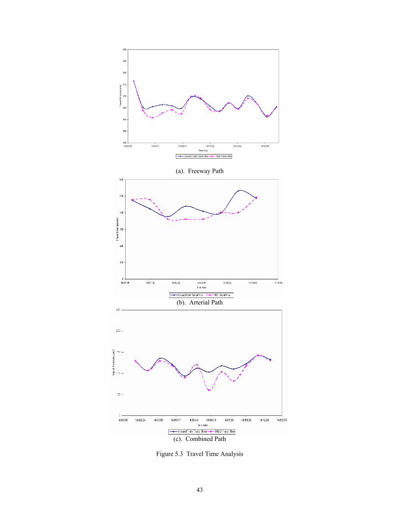
(a). Freeway Path

(b). Arterial Path

(c). Combined Path

Figure 5.3 Travel Time Analysis

43

5.5 Findings and Discussions

This section has demonstrated a framework for simulated network evaluation based on vehicle re-

identification results. Unlike most other simulation models, where vehicle tracking or re-identification is

based on individual vehicle unique ID, this study has shown an API module that enables the re-

identification of vehicles based on feature vectors. This approach also facilitates the testing and evaluation

of developed vehicle re-identification algorithms. Travel time analyses from three different paths also

suggest significant results with low estimation errors. Furthermore, this study also aims to provide optimal

aggregation interval selection depending on path characteristics and TMC’s operator viewpoint – such as

acceptable error rate.

This study needs to extend its scope by applying and implementing enhanced and more robust vehicle re-

identification algorithms for better traffic measurements estimation. Comparison among different vehicle

tracking algorithms is also an area of future study

44

CHAPTER 6 VEHICLE CLASSIFICATION

6.1 Introduction

Complete and accurate traffic information is becoming more and more available with the advance in

transportation surveillance technology. Especially, vehicle classification information can contribute to

many transportation related fields such as road pavement management, estimation of polluted emission etc.

In previous sections and chapters, it was shown that vehicle signature is function of vehicle type and traffic

conditions. By exploiting this concept, the algorithm development in vehicle classification is investigated

and corresponding results are presented

Vehicle classification is the process of vehicle type recognition based on given vehicle characteristics.

Accurate vehicle classification has many important applications in transportation. One example is road

maintenance, which is highly related to the monitoring of heavy vehicle traffic. Because trucks and

oversized vehicles exhibit distinctly different performance characteristics from passenger cars, the

continuous updating of those vehicles with respect to their share in daily traffic will help estimate the life of

current road surface and assist in the scheduling of road maintenance. Design of a toll system can also use

the same information. Moreover, by obtaining the heterogeneity of traffic flow, vehicle classification

information can lead to more reliable modeling of vehicle flow. Incorporating the information of vehicle

classification in the analysis of environmental impact is also highly desirable since different vehicle types

have different degree of airborne and noise emission. The class of vehicle is one of most important

parameters in the process of road traffic measurement. Improvement of highway safety can also benefit

from vehicle classification information, knowing that the severity of traffic accidents is highly correlated

with vehicle types. This will be discussed more in detail in the following section. To summarize, an area-

wide assessment of the component of vehicle classes in traffic is essential for more reliable and accurate

traffic analysis and modeling.

45

6.2 Background

Since early 1970s, vehicle classification has been an interested study area by many agencies and

researchers because of its importance as mentioned earlier. Especially Federal Highway Administration

(FHWA) focuses in differentiating trucks by axle counting for better road and pavement maintenance.

Davies (1986) summarized a review on early vehicle detection technologies and vehicle classification

systems. Various traffic sensors including inductive loop detector, video detector, acoustic detector, range

sensor, and infrared detector were applied in many vehicle classification studies. Inductive loop data, most

widely implemented detector system, was used by Wang et al (2001) to classify three vehicle types: heavy

vehicles, small cars, and motorcycles. Lu et al (1989) conducted k-nearest neighbor method for

categorizing vehicles into four classes using infrared detector. Video detector is also one of major detectors

used by many researchers for vehicle classification (Yuan et al, 1994; Wei et al, 1996; Gupte et al, 2002;

Avery et al, 2004). However, setting an optimal camera angle and selecting appropriate camera calibration

parameters remain issues when exploiting video data. Nooralahiyan (1997) applied signature data from

acoustic sensor and neural network method to derive four vehicle categories. A laser sensor, that returns

vehicle range and intensity information, was deployed and examined by Harlow et al (2001) for vehicle

detection and classification. However, most of the listed studies focus on detecting and distinguishing long

vehicles such as trailer and trucks from passenger cars and little consideration was paid in short vehicle

categories. In an effort to broaden study prospect on non-truck vehicle categories, Pursula et al (1994) and

Sun et al (2001, 2003) have applied loop signature data.

The proposed study aims to develop an automated vehicle classification system that can not only detect

trucks from non-truck vehicles but also can categorize small vehicles into more detailed classes.

Considering the real-time algorithm implementation in the future, the study also suggested a simple but

powerful and robust algorithm that is based on heuristic decision tree method. Especially, the multi-level

decision tree method expedites the classification system by applying selected most distinguishable vehicle

feature vectors at each step. Furthermore, a large dataset from I-405 freeway was applied to test developed

algorithm transferability. Another innovative part of this study lies in deriving vehicle classification results

in conjunction with single loop speed estimation model mentioned in earlier section. This approach will

also help to enhance the use of single loop for vehicle classification. Comparison between current FHWA

vehicle classification methods is also one of the focal points of this study.

6.3 Methodology

As shown in Table 6.1, three different vehicle classification schemes are introduced. Two categories are

based on FHWA classification. FHWA classification scheme is separated into categories depending on

whether the vehicle carries passengers or commodities. Non-passenger vehicles are further subdivided by

46

number of axles and number of units, including both power and trailer units. The difference between

FHWA I and FHWA II category is in class 2 and 3. Because automatic vehicle classifiers have difficulty

distinguishing class 3 from class 2, these two classes may be combined into class 2, which is FHWA II

category. The last category, UCI category, dedicates more to differentiate FHWA I class 3, two axle four-

tire vehicles that contains pickup truck, van and SUV. However, the signature similarity among vehicle

type in class 3 leads to classification error and therefore more sophisticated classification procedure is

required at this stage.

Heuristic decision tree method, comparable to sequential screening approach, is deployed for vehicle

classification model development. The advantage of suggested model is its simplicity, which is one of the

most important elements for fast algorithm computation process. This feature will also contribute on

possible future real-time algorithm implementation. This is very significant from both practice and

research aspects. Sequential splitting approach is based on threshold values selected from corresponding

feature vector distribution of each vehicle class. This sequential approach helps to reduce the dimension of

possible vehicle classes and therefore minimize the misclassification rate. At each step different vehicle

features, which will most distinguish one vehicle class from others, were deployed. It was shown that

vehicle length is the most dominant factor in distinguishing vehicle classes. Similar to vehicle grouping

module in previous section, DOS and SP are then used for further classification among similar vehicle

length groups. Other variables such as maximum magnitude and entropies are all applied for detailed

classifications. Figure 6.1 depicts above mentioned classification process.

47

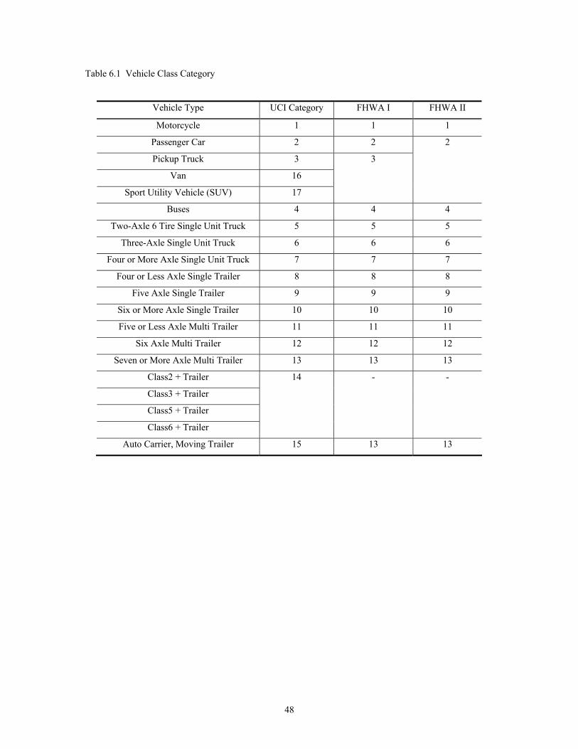
Table 6.1 Vehicle Class Category

Vehicle Type UCI Category FHWA I FHWA II

Motorcycle 1 1 1

Passenger Car 2 2

Pickup Truck 3

Van 16

Sport Utility Vehicle (SUV) 17

3

2

Buses 4 4 4

Two-Axle 6 Tire Single Unit Truck 5 5 5

Three-Axle Single Unit Truck 6 6 6

Four or More Axle Single Unit Truck 7 7 7

Four or Less Axle Single Trailer 8 8 8

Five Axle Single Trailer 9 9 9

Six or More Axle Single Trailer 10 10 10

Five or Less Axle Multi Trailer 11 11 11

Six Axle Multi Trailer 12 12 12

Seven or More Axle Multi Trailer 13 13 13

Class2 + Trailer

Class3 + Trailer

Class5 + Trailer

Class6 + Trailer

14 - -

Auto Carrier, Moving Trailer 15 13 13

48

Figure 6.1 Vehicle Classification Flow Chart

6.4 Result Analysis

6.4.1 Dataset Description

In this study, two datasets, calibration and testing, were used and manually verified for vehicle

classification. The calibration dataset consists of vehicle signature data collected from 14:00 to 14:30 PM

on I-405 at Sand Canyon and Laguna Canyon. Data from Laguna canyon at morning peak period was

applied for testing dataset. This will satisfy for model transferability testing at different time of the day. In

addition, because double loop configuration was used, single loop speed estimation can also be verified.

Datasets used in this study are illustrated in Table 6.2.

49

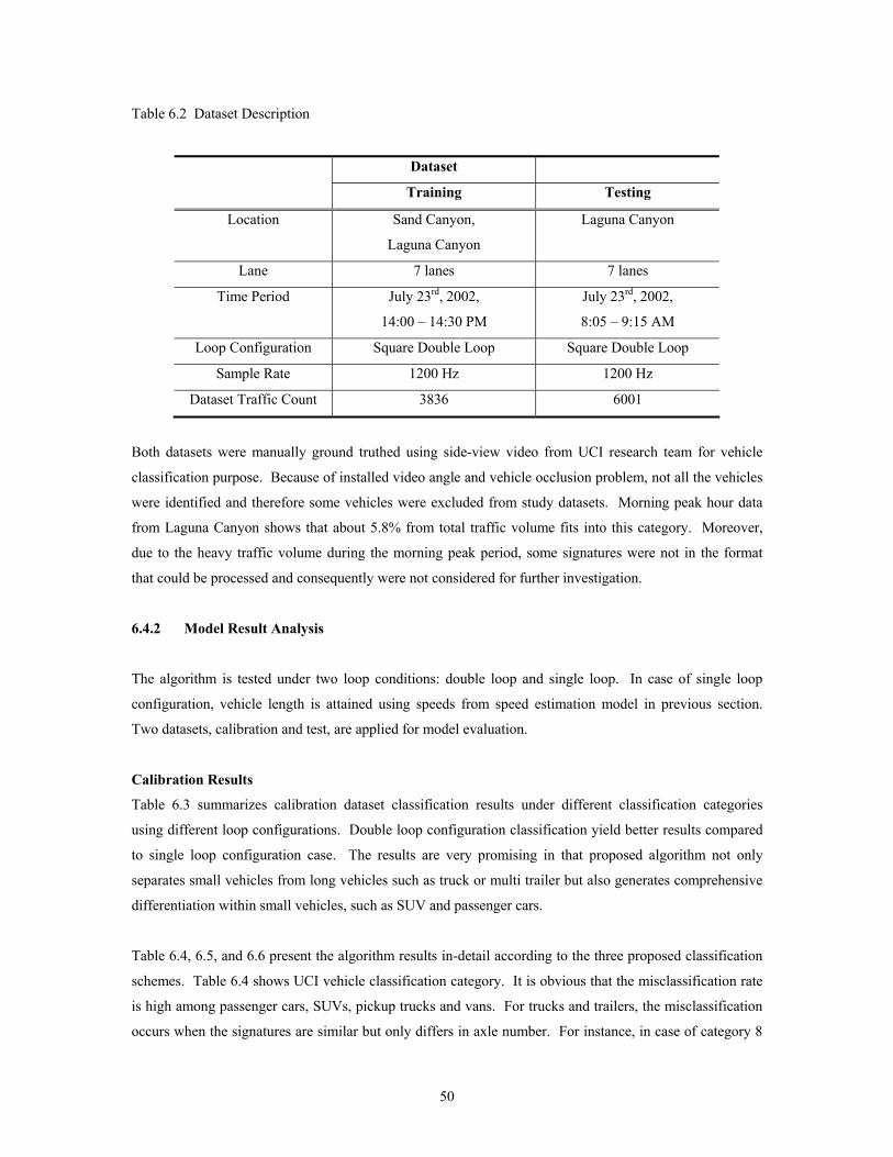
Table 6.2 Dataset Description

Dataset

Training Testing

Location Sand Canyon,

Laguna Canyon

Laguna Canyon

Lane 7 lanes 7 lanes

Time Period July 23rd, 2002,

14:00 – 14:30 PM

July 23rd, 2002,

8:05 – 9:15 AM

Loop Configuration Square Double Loop Square Double Loop

Sample Rate 1200 Hz 1200 Hz

Dataset Traffic Count 3836 6001

Both datasets were manually ground truthed using side-view video from UCI research team for vehicle

classification purpose. Because of installed video angle and vehicle occlusion problem, not all the vehicles

were identified and therefore some vehicles were excluded from study datasets. Morning peak hour data

from Laguna Canyon shows that about 5.8% from total traffic volume fits into this category. Moreover,

due to the heavy traffic volume during the morning peak period, some signatures were not in the format

that could be processed and consequently were not considered for further investigation.

6.4.2 Model Result Analysis

The algorithm is tested under two loop conditions: double loop and single loop. In case of single loop

configuration, vehicle length is attained using speeds from speed estimation model in previous section.

Two datasets, calibration and test, are applied for model evaluation.

Calibration Results

Table 6.3 summarizes calibration dataset classification results under different classification categories

using different loop configurations. Double loop configuration classification yield better results compared

to single loop configuration case. The results are very promising in that proposed algorithm not only

separates small vehicles from long vehicles such as truck or multi trailer but also generates comprehensive

differentiation within small vehicles, such as SUV and passenger cars.

Table 6.4, 6.5, and 6.6 present the algorithm results in-detail according to the three proposed classification

schemes. Table 6.4 shows UCI vehicle classification category. It is obvious that the misclassification rate

is high among passenger cars, SUVs, pickup trucks and vans. For trucks and trailers, the misclassification

occurs when the signatures are similar but only differs in axle number. For instance, in case of category 8

50

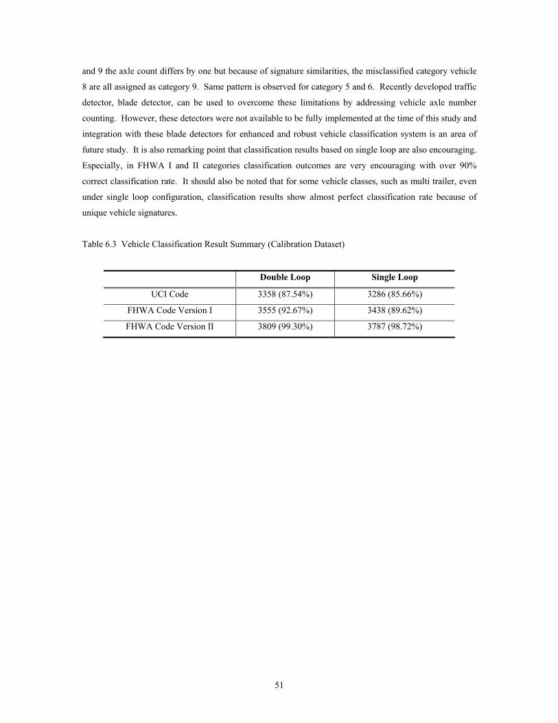
and 9 the axle count differs by one but because of signature similarities, the misclassified category vehicle

8 are all assigned as category 9. Same pattern is observed for category 5 and 6. Recently developed traffic

detector, blade detector, can be used to overcome these limitations by addressing vehicle axle number

counting. However, these detectors were not available to be fully implemented at the time of this study and

integration with these blade detectors for enhanced and robust vehicle classification system is an area of

future study. It is also remarking point that classification results based on single loop are also encouraging.

Especially, in FHWA I and II categories classification outcomes are very encouraging with over 90%

correct classification rate. It should also be noted that for some vehicle classes, such as multi trailer, even

under single loop configuration, classification results show almost perfect classification rate because of

unique vehicle signatures.

Table 6.3 Vehicle Classification Result Summary (Calibration Dataset)

Double Loop Single Loop

UCI Code 3358 (87.54%) 3286 (85.66%)

FHWA Code Version I 3555 (92.67%) 3438 (89.62%)

FHWA Code Version II 3809 (99.30%) 3787 (98.72%)

51

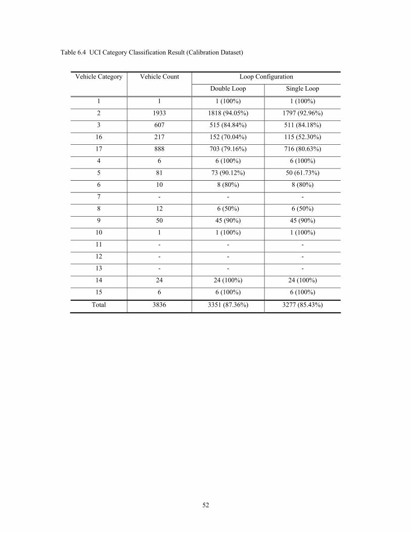
Table 6.4 UCI Category Classification Result (Calibration Dataset)

Loop Configuration Vehicle Category Vehicle Count

Double Loop Single Loop

1 1 1 (100%) 1 (100%)

2 1933 1818 (94.05%) 1797 (92.96%)

3 607 515 (84.84%) 511 (84.18%)

16 217 152 (70.04%) 115 (52.30%)

17 888 703 (79.16%) 716 (80.63%)

4 6 6 (100%) 6 (100%)

5 81 73 (90.12%) 50 (61.73%)

6 10 8 (80%) 8 (80%)

7 - - -

8 12 6 (50%) 6 (50%)

9 50 45 (90%) 45 (90%)

10 1 1 (100%) 1 (100%)

11 - - -

12 - - -

13 - - -

14 24 24 (100%) 24 (100%)

15 6 6 (100%) 6 (100%)

Total 3836 3351 (87.36%) 3277 (85.43%)

52

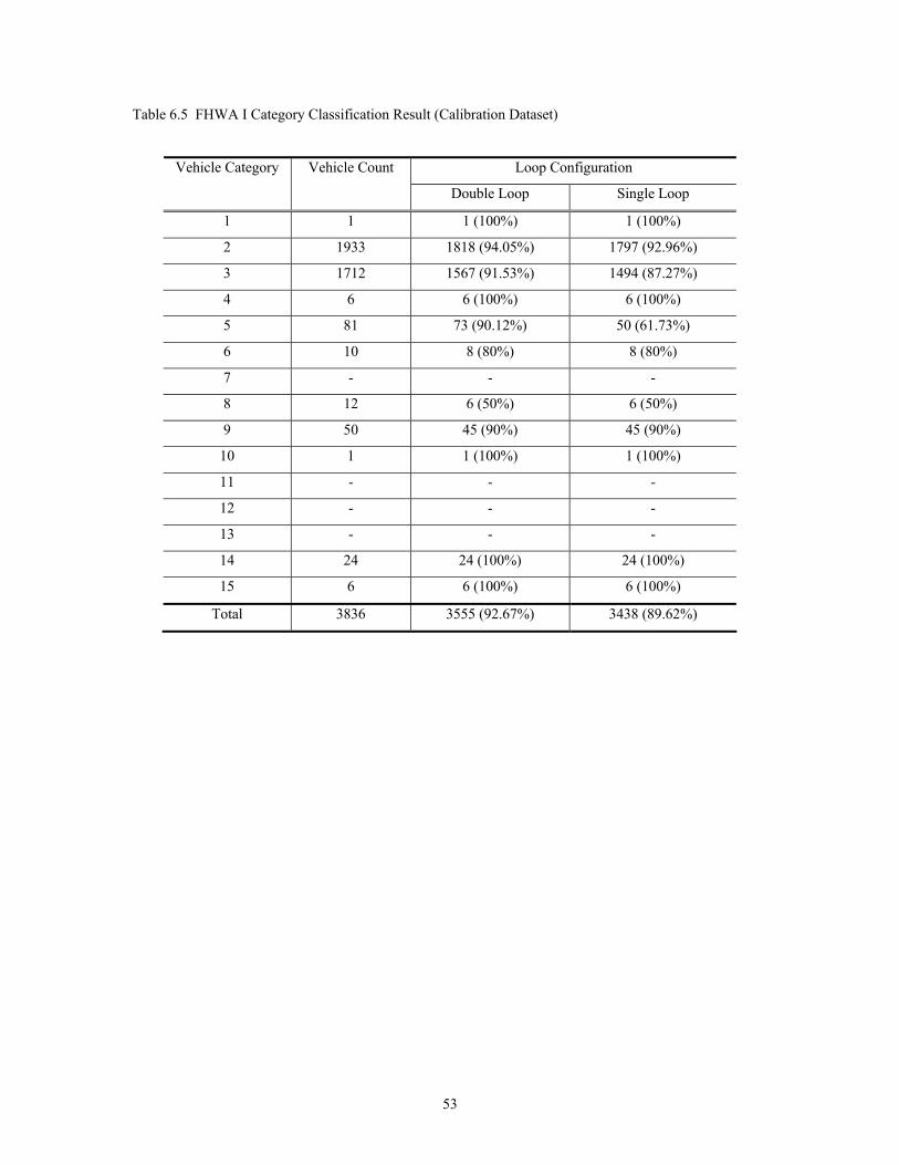
Table 6.5 FHWA I Category Classification Result (Calibration Dataset)

Loop Configuration Vehicle Category Vehicle Count

Double Loop Single Loop

1 1 1 (100%) 1 (100%)

2 1933 1818 (94.05%) 1797 (92.96%)

3 1712 1567 (91.53%) 1494 (87.27%)

4 6 6 (100%) 6 (100%)

5 81 73 (90.12%) 50 (61.73%)

6 10 8 (80%) 8 (80%)

7 - - -

8 12 6 (50%) 6 (50%)

9 50 45 (90%) 45 (90%)

10 1 1 (100%) 1 (100%)

11 - - -

12 - - -

13 - - -

14 24 24 (100%) 24 (100%)

15 6 6 (100%) 6 (100%)

Total 3836 3555 (92.67%) 3438 (89.62%)

53

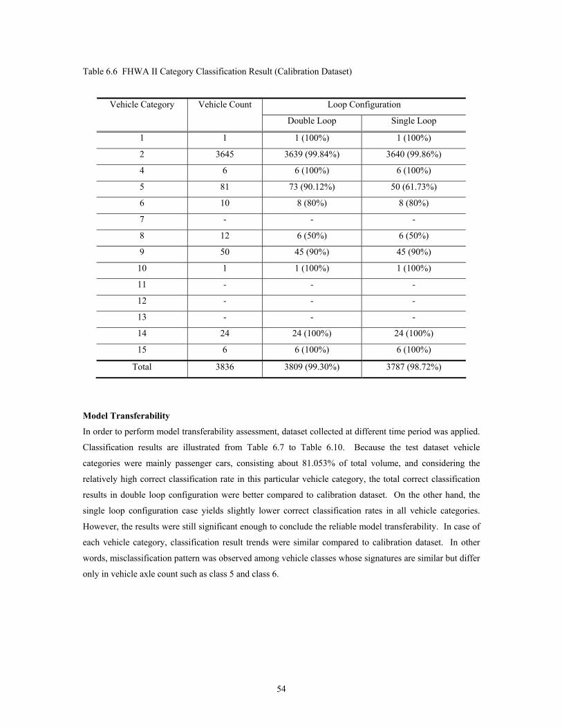
Table 6.6 FHWA II Category Classification Result (Calibration Dataset)

Loop Configuration Vehicle Category Vehicle Count

Double Loop Single Loop

1 1 1 (100%) 1 (100%)

2 3645 3639 (99.84%) 3640 (99.86%)

4 6 6 (100%) 6 (100%)

5 81 73 (90.12%) 50 (61.73%)

6 10 8 (80%) 8 (80%)

7 - - -

8 12 6 (50%) 6 (50%)

9 50 45 (90%) 45 (90%)

10 1 1 (100%) 1 (100%)

11 - - -

12 - - -

13 - - -

14 24 24 (100%) 24 (100%)

15 6 6 (100%) 6 (100%)

Total 3836 3809 (99.30%) 3787 (98.72%)

Model Transferability

In order to perform model transferability assessment, dataset collected at different time period was applied.

Classification results are illustrated from Table 6.7 to Table 6.10. Because the test dataset vehicle

categories were mainly passenger cars, consisting about 81.053% of total volume, and considering the

relatively high correct classification rate in this particular vehicle category, the total correct classification

results in double loop configuration were better compared to calibration dataset. On the other hand, the

single loop configuration case yields slightly lower correct classification rates in all vehicle categories.

However, the results were still significant enough to conclude the reliable model transferability. In case of

each vehicle category, classification result trends were similar compared to calibration dataset. In other

words, misclassification pattern was observed among vehicle classes whose signatures are similar but differ

only in vehicle axle count such as class 5 and class 6.

54

Table 6.7 Vehicle Classification Result Summary (Test Dataset)

Double Loop Single Loop

UCI Code 5384 (89.72%) 4893 (81.53%)

FHWA Code Version I 5543 (92.37%) 5051 (84.17%)

FHWA Code Version II 5937 (98.94%) 5864 (97.72%)

55

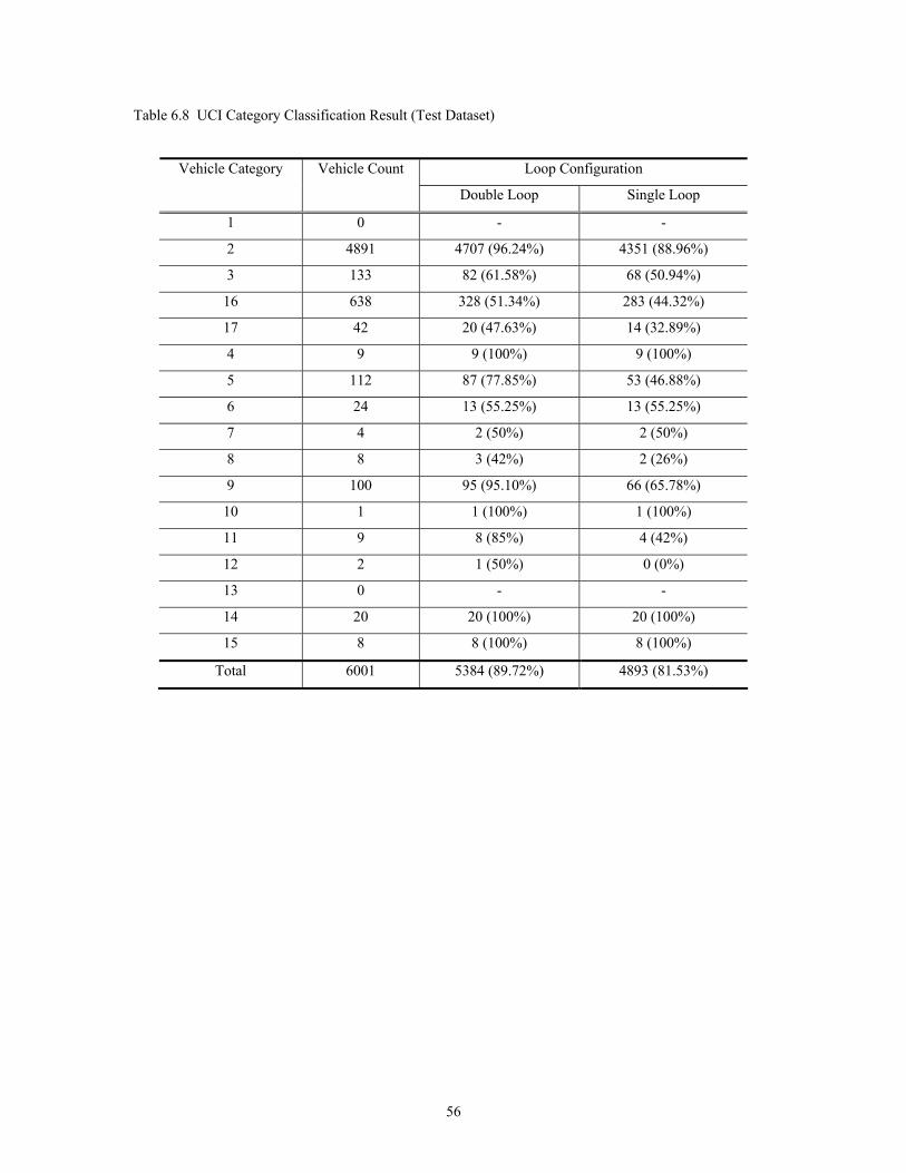
Table 6.8 UCI Category Classification Result (Test Dataset)

Loop Configuration Vehicle Category Vehicle Count

Double Loop Single Loop

1 0 - -

2 4891 4707 (96.24%) 4351 (88.96%)

3 133 82 (61.58%) 68 (50.94%)

16 638 328 (51.34%) 283 (44.32%)

17 42 20 (47.63%) 14 (32.89%)

4 9 9 (100%) 9 (100%)

5 112 87 (77.85%) 53 (46.88%)

6 24 13 (55.25%) 13 (55.25%)

7 4 2 (50%) 2 (50%)

8 8 3 (42%) 2 (26%)

9 100 95 (95.10%) 66 (65.78%)

10 1 1 (100%) 1 (100%)

11 9 8 (85%) 4 (42%)

12 2 1 (50%) 0 (0%)

13 0 - -

14 20 20 (100%) 20 (100%)

15 8 8 (100%) 8 (100%)

Total 6001 5384 (89.72%) 4893 (81.53%)

56

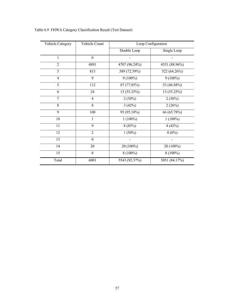
Table 6.9 FHWA Category Classification Result (Test Dataset)

Loop Configuration Vehicle Category Vehicle Count

Double Loop Single Loop

1 0 - -

2 4891 4707 (96.24%) 4351 (88.96%)

3 813 589 (72.39%) 522 (64.26%)

4 9 9 (100%) 9 (100%)

5 112 87 (77.85%) 53 (46.88%)

6 24 13 (55.25%) 13 (55.25%)

7 4 2 (50%) 2 (50%)

8 8 3 (42%) 2 (26%)

9 100 95 (95.10%) 66 (65.78%)

10 1 1 (100%) 1 (100%)

11 9 8 (85%) 4 (42%)

12 2 1 (50%) 0 (0%)

13 0 - -

14 20 20 (100%) 20 (100%)

15 8 8 (100%) 8 (100%)

Total 6001 5543 (92.37%) 5051 (84.17%)

57

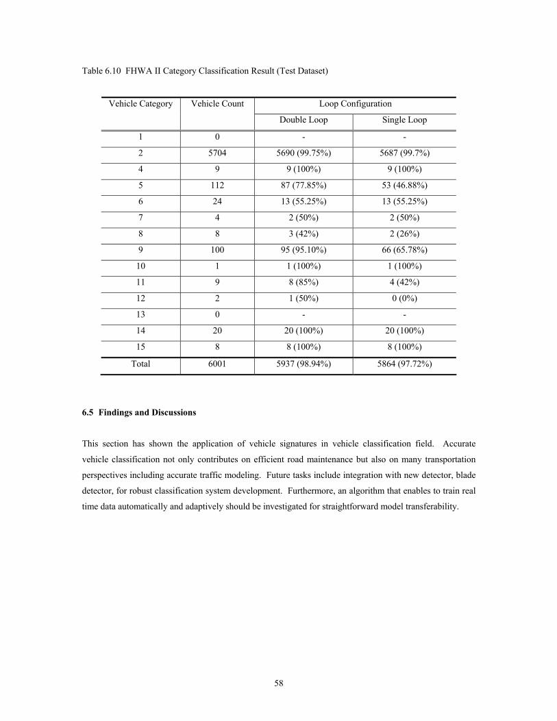
Table 6.10 FHWA II Category Classification Result (Test Dataset)

Loop Configuration Vehicle Category Vehicle Count

Double Loop Single Loop

1 0 - -

2 5704 5690 (99.75%) 5687 (99.7%)

4 9 9 (100%) 9 (100%)

5 112 87 (77.85%) 53 (46.88%)

6 24 13 (55.25%) 13 (55.25%)

7 4 2 (50%) 2 (50%)

8 8 3 (42%) 2 (26%)

9 100 95 (95.10%) 66 (65.78%)

10 1 1 (100%) 1 (100%)

11 9 8 (85%) 4 (42%)

12 2 1 (50%) 0 (0%)

13 0 - -

14 20 20 (100%) 20 (100%)

15 8 8 (100%) 8 (100%)

Total 6001 5937 (98.94%) 5864 (97.72%)

6.5 Findings and Discussions

This section has shown the application of vehicle signatures in vehicle classification field. Accurate

vehicle classification not only contributes on efficient road maintenance but also on many transportation

perspectives including accurate traffic modeling. Future tasks include integration with new detector, blade

detector, for robust classification system development. Furthermore, an algorithm that enables to train real

time data automatically and adaptively should be investigated for straightforward model transferability.

58

CHAPTER 7 CONCLUSION AND FUTURE RESEARCH

7.1 Summary of Findings

Although a variety of sensor technologies have been developed and tested for tracking individual vehicles

on transportation networks, the proposed anonymous vehicle tracking system utilizing vehicle feature

vectors provides significant advantages since it uses existing field equipment and is free from privacy

concerns. Moreover, the use of existing loop infrastructure harnesses the full potential of investments

already made and facilitates the ability for immediate field implementation. Field investigation of the

vehicle reidentification systems for a single roadway intersection and a freeway section on I-405 detector

Testbed in the City of Irvine, California, has shown the potential for extension to multiple section

implementations.

This study has presented a framework for studying the feasibility of an anonymous vehicle tracking system

for real-time freeway and arterial traffic surveillance and performance measurement. The potential

feasibility of such an approach was demonstrated by simulation experiments for a freeway and signalized

arterial operated by actuated traffic signal controls. Synthetic vehicle signatures were generated to evaluate

the proposed tracking algorithm under the simulation environment. The PARAMICS microscopic

simulation model was used to investigate the proposed vehicle tracking algorithm. The findings of this

study can serve as a logical and necessary precursor to possible field implementation of the proposed

system in freeway and arterial network. It is also believed that the proposed method for evaluating a traffic

surveillance system using microscopic simulation in this study can offer a valuable tool to operating

agencies interested in real-time congestion monitoring, traveler information, control, and system

evaluation. Furthermore, the automatic vehicle classification system developed in this study showed very

encouraging results.

7.2 Future Research

To fully exploit the benefits of the new generation of Intelligent Transportation Systems now widely under

development, including applications for performance measurement and homeland security, more accurate

and appropriate real-time traffic data need to be collected from the urban highway transportation network

and communicated to traffic management centers, traffic operations personnel, travelers, and other

agencies. Future research should now deploy and investigate at a corridor level the anonymous vehicle

tracking techniques that have been pioneered by the authors in previous PATH research. The objective of

such deployment would be to investigate and demonstrate real-time freeway and arterial performance

measurement in a major real-world setting. This research under TO 4159 emphasized microscopic

59

simulation in conjunction with individual intersection and freeway segment field implementations to

develop and assess methods for tracking vehicles across multiple detector stations in a traffic network,

based on real-time acquisition of vehicle inductive signatures, in order to provide improved freeway and

arterial (and transit) performance measures to the Caltrans PeMS. Ultimately, however, the utility and

effectiveness of such new network-based methods can only be judged through large-scale field

implementation.

60

REFERENCES

1. Banks, J., Carson, J. S., and Nelson, B. L. Discrete Event System Simulation. 2nd Edition Prentice Hall

2. Chu, L., Liu X., Oh, J., Recker, W. (2004) A Calibration Procedure for Microscopic Traffic

Simulation. Presented at the 83rd Annual Meeting of Transportation Research Board.

3. Chu, L., Liu X., Recker, W., Hague S. (2003) Evaluation of Potential ITS Strategies under Non-

recurrent Congestion Using Microscopic Simulation, California PATH Working Paper UCB-ITS-

PWP-2003-2

4. Davies, P. (1986) Vehicle Detection and Classification. Information Technology Application in

Transport. VNU Science Press, Haarlem, the Netherlands, pp 11-40

5. Duncan G.I. (1995) PARAMICS wide area microscopic simulation of ATT and traffic management,

Proceedings of the 28th International Symposium on Automotive Technology and Automation

(ISATA), Stuggartt, Germany, 475 – 484

6. Harlow, C., and Peng, S. (2001) Automatic Vehicle Classification System with Range Sensors.

Transportation Research Part C Vol 9, pp 231 – 247.

7. Hogg, R.V., and Tanis, E.A. (1993) Probability and Statistical Inference. Prentice Hall

8. Gault and Taylor 1977, Gault, H.E., and Taylor, I.G. (1977) The use of output from vehicle detectors

to access delay in computer-controlled area traffic control systems. Res. Rep. 31, Transp. Operation

Res. Gp., University of Newcastle upon Tyne, U.K.

9. Gupte, S., Masoud, O., Martin R.F.K., and Papanikolopoulos, N.P. (2002) Detection and

Classification of Vehicles. IEEE Transactions on Intelligent Transportation Systems, Vol 3, No 1, pp

37-47.

10. Kaufman, L. and Rousseeuw, P.J. (1990) Finding Groups in Data: An Introduction to Cluster

Analysis. Wiley, New York.

11. Kwon, J., Varaiya, P. and Skabardonis, A. (2003) "Estimation of Truck Traffic Volume from Single

Loop Detector Outputs Using Lane-to-lane Speed Correlation," California PATH working paper UCB-

ITS-PWP-2003-11

12. Lee, D. (1998) PARAMICS Simulations at the California ATMIS Testbed: A Benchmark Ananysis.

Working Paper, Institute of Transportation Studies, University of California, Irvine.

13. Lu, Y. (1989) Vehicle Classification Using Infrared Image Analysis. Journal of Transportation

Engineering ASCE, Vol. 118. No. 2., pp. 223-240

14. Nooralahiyan, A.Y. Dougherty, M., McKeown, D., and Kirby, H.R. (1997) A Field Trial of Acoustic

Signature Analysis for Vehicle Classification. Transportation Research Part C, Vol. 5, No.3, pp. 165-

177

15. Oh, S., Ritchie, S. G., and Oh, C. (2002) Real Time Traffic Measurement from Single Loop Inductive

Signatures. Transportation Research Board 1804: 98-106.

61

62

16. Oh, C. (2003) Anonymous Vehicle Tracking for Real-Time Traffic Performance Measures. Ph.D

Dissertation, University of California, Irvine.

17. Park, S., and Ritchie, S. G. (2004) Exploring the Relationship between Freeway Speed Variance, Lane

Changing, and Vehicle Heterogeneity. Presented at the 83rd Annual Meeting of Transportation

Research Board.

18. Park, S. (2004) Vehicle Monitoring for Traffic Surveillance and Performance using Multi-Sensor Data

Fusion. Ph.D Dissertation, University of California, Irvine.

19. Pursula, M. and Pikkarainen, P. (1994) A Neural Network Approach to Vehicle Classification with

Double Induction Loops. Proceedings of the 17th ARRB Conference. Part 4. pp. 29-44

20. Quadstone Ltd. (2003) PARAMICS Traffic Simulation Modeller V4.2 Reference Manual

21. Quadstone Ltd. (2003) PARAMICS Traffic Simulation Modeller V4.2 User Guide

22. Ritchie, S. G., Sun, C., Oh, S., and Oh, C. (2001) Section Related Measures of Traffic System

Performance : Prototype Field Implementation. California PATH Research Report, UCB-ITS-PRR-

2001-32

23. Ritchie, S. G., Park, S., Oh, C., and Sun, C. (2002) Field Investigation of Advanced Vehicle

Reidentification Techniques and Detector Technologies – Phase I. California PATH Research Report,

UCB-ITS-PRR-2002-15

24. Sisiopiku and Rouphail, 1994, Sisiopiku, V.P., and Rouphail, N.M. (1994) Travel time estimation

from loop detector data for advanced traveler information system applications. Technical report in

support of ADVANCE project, Illinois university transportation research consortium, Chicago, Ill.

25. Sun, C., Ritchie, S.G., Tsai, W., and R. Jayakrishnan. (1999) Use of Vehicle Signature Analysis and

Lexicographic Optimization for Vehicle Reidentification on Freeways. Transportation Research, Part

C, Vol 7, pp 167-185

26. Sun, C., Ritchie, S.G., and Oh, S. (2001) Inductive Classifying Artificial Network for Vehicle Type

Categorization. Presented at the 80th Annual Meeting Transportation Research Board.

27. Sun, C., Ritchie, S. G., and Oh, S. (2003) Inductive Classifying Artificial Network for Vehicle Type

Categorization. Journal of Computer-Aided Civil and Infrastructure Engineering, Vol 18. pp161-172.

28. Wang, Y., and Nihan, N. L. (2001) Dynamic Estimation of Freeway Large Truck Volumes based on

Single-Loop Measurements. Presented at the 80th Annual Meeting of Transportation Research Board.

29. Wei, C., Chang, C.C., and Wang, S.S. (1996) Vehicle Classification Using Advanced Technologies.

Transportation Research Record 1551, pp. 45-50

30. Xie et al 2001, Xie, C., Cheu, R.L., and Lee. D. (2001) Calibration-free arterial link speed estimation

model using loop data. Journal of Transportation Engineering ASCE 127(6), 507-514.

31. Yuan, X., Lu, Y.J., and Sarraf, S. (1994) Computer Vision System for Automatic Vehicle

Classification. Journal of Transportation Engineering ASCE, Vol. 120, No. 6, pp. 861-876

32. Zhang 1998, Zhang, H.M. (1998) A link journey speed model for arterial traffic. Transportation

Research Record 1676, TRB, National Research Council, Washington, D.C., pp.109-115