MATH1510

Financial Mathematics I

Jitse NiesenUniversity of Leeds

January – May 2012

Description of the module

This is the description of the module as it appears in the module catalogue.

Objectives

Introduction to mathematical modelling of financial and insurance markets withparticular emphasis on the time-value of money and interest rates. Introductionto simple financial instruments. This module covers a major part of the Facultyand Institute of Actuaries CT1 syllabus (Financial Mathematics, core technical).

Learning outcomes

On completion of this module, students should be able to understand the timevalue of money and to calculate interest rates and discount factors. They shouldbe able to apply these concepts to the pricing of simple, fixed-income financialinstruments and the assessment of investment projects.

Syllabus

• Interest rates. Simple interest rates. Present value of a single futurepayment. Discount factors.

• Effective and nominal interest rates. Real and money interest rates. Com-pound interest rates. Relation between the time periods for compoundinterest rates and the discount factor.

• Compound interest functions. Annuities and perpetuities.

• Loans.

• Introduction to fixed-income instruments. Generalized cashflow model.

• Net present value of a sequence of cashflows. Equation of value. Internalrate of return. Investment project appraisal.

• Examples of cashflow patterns and their present values.

• Elementary compound interest problems.

MATH1510 i

Reading list

These lecture notes are based on the following books:

1. Samuel A. Broverman, Mathematics of Investment and Credit, 4th ed.,ACTEX Publications, 2008. ISBN 978-1-56698-657-1.

2. The Faculty of Actuaries and Institute of Actuaries, Subject CT1: Finan-cial Mathematics, Core Technical. Core reading for the 2009 examinations.

3. Stephen G. Kellison, The Theory of Interest, 3rd ed., McGraw-Hill, 2009.ISBN 978-007-127627-6.

4. John McCutcheon and William F. Scott, An Introduction to the Mathe-matics of Finance, Elsevier Butterworth-Heinemann, 1986. ISBN 0-7506-0092-6.

5. Petr Zima and Robert L. Brown, Mathematics of Finance, 2nd ed., Schaum’sOutline Series, McGraw-Hill, 1996. ISBN 0-07-008203.

The syllabus for the MATH1510 module is based on Units 1–9 and Unit 11 ofbook 2. The remainder forms the basis of MATH2510 (Financial Mathemat-ics II). The book 2 describes the first exam that you need to pass to become anaccredited actuary in the UK. It is written in a concise and perhaps dry style.

These lecture notes are largely based on Book 4. Book 5 contains many exer-cises, but does not go quite as deep. Book 3 is written from a U.S. perspective, sothe terminology is slightly different, but it has some good explanations. Book 1is written by a professor from a U.S./Canadian background and is particularlygood in making connections to applications.

All these books are useful for consolidating the course material. They allowyou to gain background knowledge and to try your hand at further exercises.However, the lecture notes cover the entire syllabus of the module.

ii MATH1510

Organization for 2011/12

Lecturer Jitse Niesen

E-mail jitse@maths.leeds.ac.uk

Office Mathematics 8.22f

Telephone 35870 (from outside: 0113 3435870)

Lectures Tuesdays 10:00 – 11:00 in Roger Stevens LT 20Wednesdays 12:00 – 13:00 in Roger Stevens LT 25Fridays 14:00 – 15:00 in Roger Stevens LT 17

Example classes Mondays in weeks 3, 5, 7, 9 and 11,see your personal timetable for time and room.

Tutors Niloufar Abourashchi, Zhidi Du, James Fung, and TongyaWang.

Office hours Tuesdays . . . . . . . . (to be determined)or whenever you find the lecturer and he has time.

Course work There will be five sets of course work. Put your work inyour tutor’s pigeon hole on Level 8 of School of Mathemat-ics. Due dates are Wednesday 1 February, 15 February,29 February, 14 March and 25 April.

Late work One mark (out of ten) will be deducted for every day.

Copying Collaboration is allowed (even encouraged), copying not.See the student handbook for details.

Exam The exam will take place in the period 14 May – 30 May;exact date and location to be announced.

Assessment The course work counts for 15%, the exam for 85%.

Lecture notes These notes and supporting materials are available in theBlackboard VLE.

MATH1510 iii

iv MATH1510

Chapter 1

The time value of money

Interest is the compensation one gets for lending a certain asset. For instance,suppose that you put some money on a bank account for a year. Then, the bankcan do whatever it wants with that money for a year. To reward you for that,it pays you some interest.

The asset being lent out is called the capital. Usually, both the capital andthe interest is expressed in money. However, that is not necessary. For instance,a farmer may lend his tractor to a neighbour, and get 10% of the grain harvestedin return. In this course, the capital is always expressed in money, and in thatcase it is also called the principal.

1.1 Simple interest

Interest is the reward for lending the capital to somebody for a period of time.There are various methods for computing the interest. As the name implies,simple interest is easy to understand, and that is the main reason why we talkabout it here. The idea behind simple interest is that the amount of interestis the product of three quantities: the rate of interest, the principal, and theperiod of time. However, as we will see at the end of this section, simple interestsuffers from a major problem. For this reason, its use in practice is limited.

Definition 1.1.1 (Simple interest). The interest earned on a capital C lentover a period n at a rate i is niC.

Example 1.1.2. How much interest do you get if you put 1000 pounds for twoyears in a savings acount that pays simple interest at a rate of 9% per annum?And if you leave it in the account for only half ar year?

Answer. If you leave it for two years, you get

2 · 0.09 · 1000 = 180

pounds in interest. If you leave it for only half a year, then you get 12 ·0.09·1000 =

45 pounds.

As this example shows, the rate of interest is usually quoted as a percentage;9% corresponds to a factor of 0.09. Furthermore, you have to be careful thatthe rate of interest is quoted using the same time unit as the period. In this

MATH1510 1

example, the period is measured in years, and the interest rate is quoted perannum (“per annum” is Latin for “per year”). These are the units that are usedmost often. In Section 1.5 we will consider other possibilities.

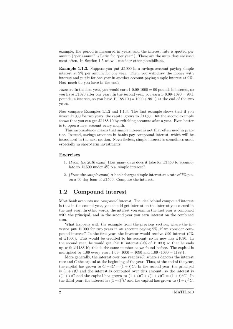
Example 1.1.3. Suppose you put £1000 in a savings account paying simpleinterest at 9% per annum for one year. Then, you withdraw the money withinterest and put it for one year in another account paying simple interest at 9%.How much do you have in the end?

Answer. In the first year, you would earn 1·0.09·1000 = 90 pounds in interest, soyou have £1090 after one year. In the second year, you earn 1 ·0.09 ·1090 = 98.1pounds in interest, so you have £1188.10 (= 1090 + 98.1) at the end of the twoyears.

Now compare Examples 1.1.2 and 1.1.3. The first example shows that if youinvest £1000 for two years, the capital grows to £1180. But the second exampleshows that you can get £1188.10 by switching accounts after a year. Even betteris to open a new account every month.

This inconsistency means that simple interest is not that often used in prac-tice. Instead, savings accounts in banks pay compound interest, which will beintroduced in the next section. Nevertheless, simple interest is sometimes used,especially in short-term investments.

Exercises

1. (From the 2010 exam) How many days does it take for £1450 to accumu-late to £1500 under 4% p.a. simple interest?

2. (From the sample exam) A bank charges simple interest at a rate of 7% p.a.on a 90-day loan of £1500. Compute the interest.

1.2 Compound interest

Most bank accounts use compound interest. The idea behind compound interestis that in the second year, you should get interest on the interest you earned inthe first year. In other words, the interest you earn in the first year is combinedwith the principal, and in the second year you earn interest on the combinedsum.

What happens with the example from the previous section, where the in-vestor put £1000 for two years in an account paying 9%, if we consider com-pound interest? In the first year, the investor would receive £90 interest (9%of £1000). This would be credited to his account, so he now has £1090. Inthe second year, he would get £98.10 interest (9% of £1090) so that he endsup with £1188.10; this is the same number as we found before. The capital ismultiplied by 1.09 every year: 1.09 · 1000 = 1090 and 1.09 · 1090 = 1188.1.

More generally, the interest over one year is iC, where i denotes the interestrate and C the capital at the beginning of the year. Thus, at the end of the year,the capital has grown to C + iC = (1 + i)C. In the second year, the principalis (1 + i)C and the interest is computed over this amount, so the interest isi(1 + i)C and the capital has grown to (1 + i)C + i(1 + i)C = (1 + i)2C. Inthe third year, the interest is i(1 + i)2C and the capital has grown to (1 + i)3C.

2 MATH1510

This reasoning, which can be made more formal by using complete induction,leads to the following definition.

Definition 1.2.1 (Compound interest). A capital C lent over a period n at arate i grows to (1 + i)nC.

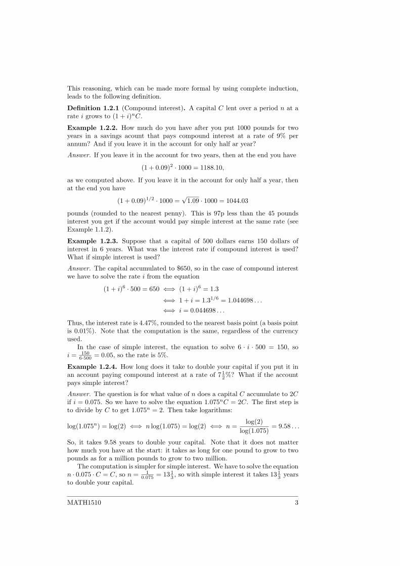
Example 1.2.2. How much do you have after you put 1000 pounds for twoyears in a savings acount that pays compound interest at a rate of 9% perannum? And if you leave it in the account for only half ar year?

Answer. If you leave it in the account for two years, then at the end you have

(1 + 0.09)2 · 1000 = 1188.10,

as we computed above. If you leave it in the account for only half a year, thenat the end you have

(1 + 0.09)1/2 · 1000 =√

1.09 · 1000 = 1044.03

pounds (rounded to the nearest penny). This is 97p less than the 45 poundsinterest you get if the account would pay simple interest at the same rate (seeExample 1.1.2).

Example 1.2.3. Suppose that a capital of 500 dollars earns 150 dollars ofinterest in 6 years. What was the interest rate if compound interest is used?What if simple interest is used?

Answer. The capital accumulated to $650, so in the case of compound interestwe have to solve the rate i from the equation

(1 + i)6 · 500 = 650 ⇐⇒ (1 + i)6 = 1.3

⇐⇒ 1 + i = 1.31/6 = 1.044698 . . .⇐⇒ i = 0.044698 . . .

Thus, the interest rate is 4.47%, rounded to the nearest basis point (a basis pointis 0.01%). Note that the computation is the same, regardless of the currencyused.

In the case of simple interest, the equation to solve 6 · i · 500 = 150, soi = 150

6·500 = 0.05, so the rate is 5%.

Example 1.2.4. How long does it take to double your capital if you put it inan account paying compound interest at a rate of 7 1

2%? What if the accountpays simple interest?

Answer. The question is for what value of n does a capital C accumulate to 2Cif i = 0.075. So we have to solve the equation 1.075nC = 2C. The first step isto divide by C to get 1.075n = 2. Then take logarithms:

log(1.075n) = log(2) ⇐⇒ n log(1.075) = log(2) ⇐⇒ n =log(2)

log(1.075)= 9.58 . . .

So, it takes 9.58 years to double your capital. Note that it does not matterhow much you have at the start: it takes as long for one pound to grow to twopounds as for a million pounds to grow to two million.

The computation is simpler for simple interest. We have to solve the equationn · 0.075 ·C = C, so n = 1

0.075 = 13 13 , so with simple interest it takes 13 1

3 yearsto double your capital.

MATH1510 3

More generally, if the interest rate is i, then the time required to double yourcapital is

n =log(2)

log(1 + i).

We can approximate the denominator by log(1 + i) ≈ i for small i; this isthe first term of the Taylor series of log(1 + i) around i = 0 (note that, as iscommon in mathematics, “log” denotes the natural logarithm). Thus, we getn ≈ log(2)

i . If instead of the interest rate i we use the percentage p = 100i, andwe approximate log(2) = 0.693 . . . by 0.72, we get

n ≈ 72p.

This is known as the rule of 72 : To calculate how many years it takes you todouble your money, you divide 72 by the interest rate expressed as a percentage.Let us return to the above example with a rate of 7 1

2%. We have p = 7 12 so we

compute 72/7 12 = 9.6, which is very close to the actual value of n = 9.58 we

computed before.The rule of 72 can already be found in a Italian book from 1494: Summa de

Arithmetica by Luca Pacioli. The use of the number 72 instead of 69.3 has twoadvantages: many numbers divide 72, and it gives a better approximation forrates above 4% (remember that the Taylor approximation is centered aroundi = 0; it turns out that it is slightly too small for rates of 5–10% and using 72instead of 69.3 compensates for this).

Remember that with simple interest, you could increase the interest you earnby withdrawing your money from the account halfway. Compound interest hasthe desirable property that this does not make a difference. Suppose that youput your money m years in one account and then n years in another account,and that both account pay compount interest at a rate i. Then, after thefirst m years, your capital has grown to (1 + i)mC. You withdraw that andput it in another account for n years, after which your capital has grown to(1 + i)n(1 + i)mC. This is the same as what you would get if you had kept thecapital in the same account for m+ n years, because

(1 + i)n(1 + i)mC = (1 + i)m+nC.

This is the reason why compound interest is used so much in practice. Unlessnoted otherwise, interest will always refer to compound interest.

Exercises

1. The rate of interest on a certain bank deposit account is 412% per annum

effective. Find the accumulation of £5000 after seven years in this account.

2. (From the sample exam) How long does it take for £900 to accumulate to£1000 under an interest rate of 4% p.a.?

4 MATH1510

0 2 4 6 8 100

0.5

1

1.5

2

2.5

time (in years)

final

cap

ital

0 5 10 150

0.5

1

1.5

2

2.5

interest rate (%)

final

cap

ital

simplecompound

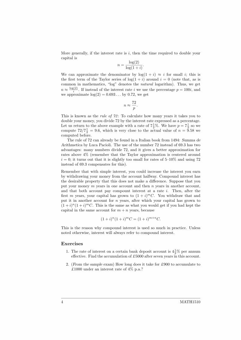
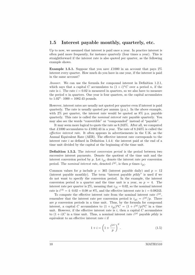
Figure 1.1: Comparison of simple interest and compound interest. The leftfigure plots the growth of capital in time at a rate of 9%. The right figure plotsthe amount of capital after 5 years for various interest rates.

1.3 Comparing simple and compound interest

Simple interest is defined by the formula “interest = inC.” Thus, in n years thecapital grows from C to C + niC = (1 + ni)C. Simple interest and compoundinterest compare as follows:

simple interest: capital after n years = (1 + ni)Ccompound interest: capital after n years = (1 + i)nC

These formulas are compared in Figure 1.1. The left plot shows how a principalof 1 pound grows under interest at 9%. The dashed line is for simple interest andthe solid curve for compound interest. We see that compound interest pays outmore in the long term. A careful comparison shows that for periods less than ayear simple interest pays out more, while compound interest pays out more if theperiod is longer than a year. This agrees with what we found before. A capitalof £1000, invested for half a year at 9%, grows to £1045 under simple interestand to £1044.03 under compound interest, while the same capital invested fortwo years grows to £1180 under simple interest and £1188.10 under compoundinterest. The difference between compound and simple interest get bigger asthe period gets longer.

This follows from the following algebraic inequalities: if i is positive, then

(1 + i)n < 1 + ni if n < 1,(1 + i)n > 1 + ni if n > 1.

These will not be proven here. However, it is easy to see that the formulasfor simple and compound interest give the same results if n = 0 and n = 1.Now consider the case n = 2. A capital C grows to (1 + 2i)C under simpleinterest and to (1 + i)2C = (1 + 2i + i2)C under compound interest. We have(1 + 2i + i2)C > (1 + 2i)C (because C is positive), so compound interest paysout more than simple interest.

The right plot in Figure 1.1 shows the final capital after putting a principalof 1 pound away for five years at varying interest rates. Again, the dashed linecorresponds to simple interest and the solid curve corresponds to compound

MATH1510 5

t = 5

= £2000.00

accumulating

t = 0

future value

discounting

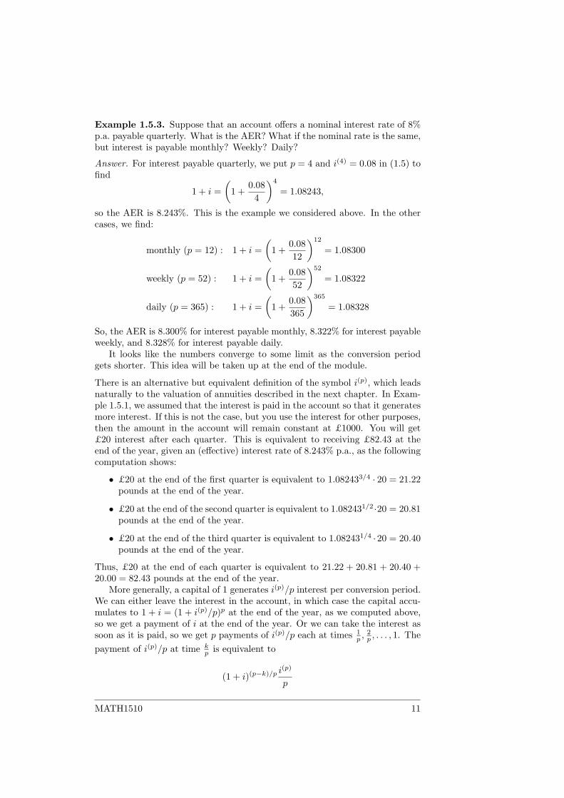
present value= £1624.24

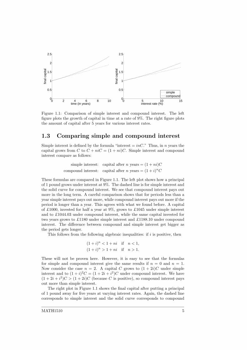
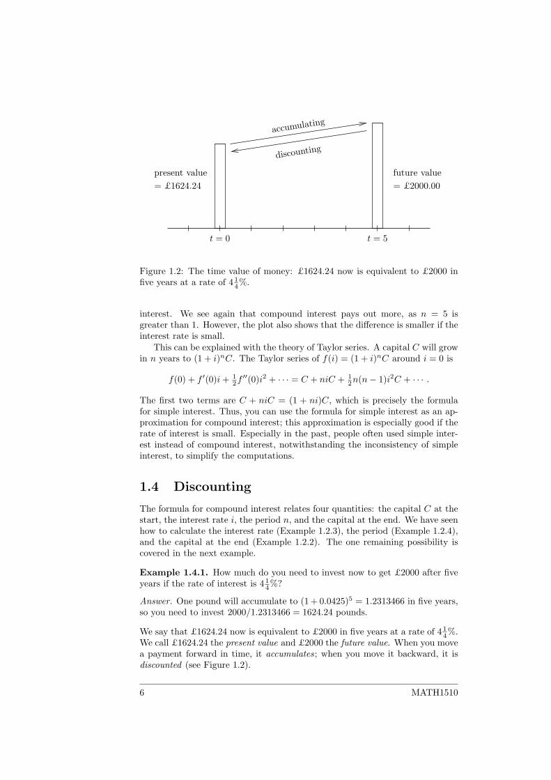
Figure 1.2: The time value of money: £1624.24 now is equivalent to £2000 infive years at a rate of 4 1

4%.

interest. We see again that compound interest pays out more, as n = 5 isgreater than 1. However, the plot also shows that the difference is smaller if theinterest rate is small.

This can be explained with the theory of Taylor series. A capital C will growin n years to (1 + i)nC. The Taylor series of f(i) = (1 + i)nC around i = 0 is

f(0) + f ′(0)i+ 12f′′(0)i2 + · · · = C + niC + 1

2n(n− 1)i2C + · · · .

The first two terms are C + niC = (1 + ni)C, which is precisely the formulafor simple interest. Thus, you can use the formula for simple interest as an ap-proximation for compound interest; this approximation is especially good if therate of interest is small. Especially in the past, people often used simple inter-est instead of compound interest, notwithstanding the inconsistency of simpleinterest, to simplify the computations.

1.4 Discounting

The formula for compound interest relates four quantities: the capital C at thestart, the interest rate i, the period n, and the capital at the end. We have seenhow to calculate the interest rate (Example 1.2.3), the period (Example 1.2.4),and the capital at the end (Example 1.2.2). The one remaining possibility iscovered in the next example.

Example 1.4.1. How much do you need to invest now to get £2000 after fiveyears if the rate of interest is 4 1

4%?

Answer. One pound will accumulate to (1 + 0.0425)5 = 1.2313466 in five years,so you need to invest 2000/1.2313466 = 1624.24 pounds.

We say that £1624.24 now is equivalent to £2000 in five years at a rate of 4 14%.

We call £1624.24 the present value and £2000 the future value. When you movea payment forward in time, it accumulates; when you move it backward, it isdiscounted (see Figure 1.2).

6 MATH1510

i

1 + i

1

t = 0

v

d

discount(by one year)

accumulate(over one year)

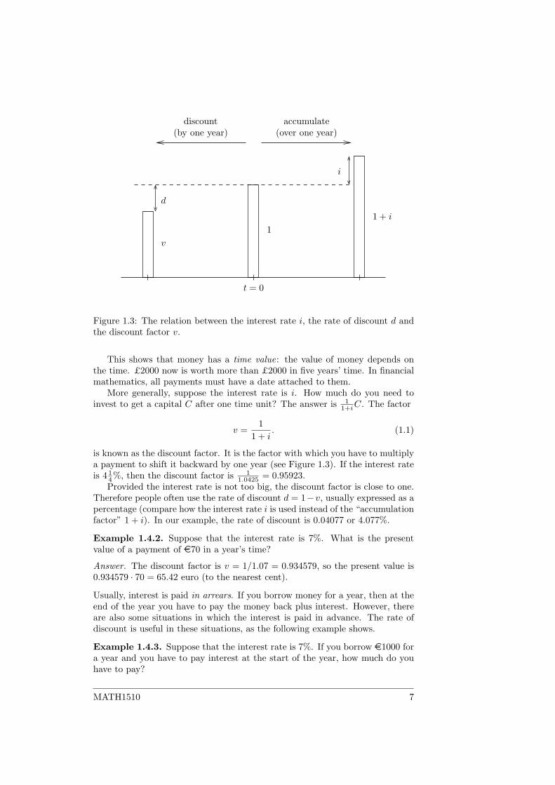
Figure 1.3: The relation between the interest rate i, the rate of discount d andthe discount factor v.

This shows that money has a time value: the value of money depends onthe time. £2000 now is worth more than £2000 in five years’ time. In financialmathematics, all payments must have a date attached to them.

More generally, suppose the interest rate is i. How much do you need toinvest to get a capital C after one time unit? The answer is 1

1+iC. The factor

v =1

1 + i. (1.1)

is known as the discount factor. It is the factor with which you have to multiplya payment to shift it backward by one year (see Figure 1.3). If the interest rateis 4 1

4%, then the discount factor is 11.0425 = 0.95923.

Provided the interest rate is not too big, the discount factor is close to one.Therefore people often use the rate of discount d = 1−v, usually expressed as apercentage (compare how the interest rate i is used instead of the “accumulationfactor” 1 + i). In our example, the rate of discount is 0.04077 or 4.077%.

Example 1.4.2. Suppose that the interest rate is 7%. What is the presentvalue of a payment of e70 in a year’s time?

Answer. The discount factor is v = 1/1.07 = 0.934579, so the present value is0.934579 · 70 = 65.42 euro (to the nearest cent).

Usually, interest is paid in arrears. If you borrow money for a year, then at theend of the year you have to pay the money back plus interest. However, thereare also some situations in which the interest is paid in advance. The rate ofdiscount is useful in these situations, as the following example shows.

Example 1.4.3. Suppose that the interest rate is 7%. If you borrow e1000 fora year and you have to pay interest at the start of the year, how much do youhave to pay?

MATH1510 7

Answer. If interest were to be paid in arrears, then you would have to pay0.07 · 1000 = 70 euros at the end of the year. However, you have to pay theinterest one year earlier. As we saw in Example 1.4.2, the equivalent amount isv · 70 = 65.42 euros.

There is another way to arrive at the answer. At the start of the year, youget e1000 from the lender but you have to pay interest immediately, so in effectyou get less from the lender. At the end of the year, you pay e1000 back. Theamount you should get at the start of the year should be equivalent to the e1000you pay at the end of the year. The discount factor is v = 1/1.07 = 0.934579,so the present value of the e1000 at the end of the year is e934.58. Thus, theinterest you have to pay is e1000− e934.58 = e65.42.

In terms of the interest rate i = 0.07 and the capital C = 1000, the first methodcalculates ivC and the second method calculates C − vC = (1 − v)C = dC.Both methods yield the same answer, so we arrive at the important relation

d = iv. (1.2)

We can check this relation algebraically. We found before, in equation (1.1),that the discount factor is

v =1

1 + i.

The rate of discount is

d = 1− v = 1− 11 + i

=i

1 + i. (1.3)

Comparing these two formulas, we find that indeed d = iv.We summarize this discussion with a formal definition of the three quantities

d, i and v.

Definition 1.4.4. The rate of interest i is the interest paid at the end of atime unit divided by the capital at the beginning of the time unit. The rateof discount d is the interest paid at the beginning of a time unit divided bythe capital at the end of the time unit. The discount factor v is the amount ofmoney one needs to invest to get one unit of capital after one time unit.

This definition concerns periods of one year (assuming that time is measured inyears). In Example 1.4.1, we found that the present value of a payment of £2000due in five years is £1624.24, if compound interest is used at a rate of 4 1

4%. Thiswas computed as 2000/(1 + 0.0425)5. The same method can be used to find thepresent value of a payment of C due in n years if compound interest is used ata rate i. The question is: which amount x accumulates to C in n years? Theformula for compound interest yields that (1 + i)nx = C, so the present value xis

C

(1 + i)n= vnC = (1− d)nC. (1.4)

This is called compound discounting, analogous with compound interest.There is another method, called simple discounting (analogous to simple

interest) or commercial discounting. This is defined as follows. The presentvalue of a payment of C due in n years, at a rate of simple discount of d, is(1− nd)C.

8 MATH1510

Simple discounting is not the same as simple interest. The present value ofa payment of C due in n years, at a rate of simple interest of i, is the amount xthat accumulates to C over n years. Simple interest is defined by C = (1+ni)x,so the present value is x = (1 + ni)−1C.

Example 1.4.5. What is the present value of £6000 due in a month assum-ing 8% p.a. simple discount? What is the corresponding rate of (compound)discount? And the rate of (compound) interest? And the rate of simple interest?

Answer. One month is 112 year, so the present value of is (1− 1

12 · 0.08) · 6000 =5960 pounds. We can compute the rate of (compound) discount d from theformula “present value = (1− d)nC”:

5960 = (1− d)1/12 · 6000 =⇒ (1− d)1/12 = 59606000 = 0.993333

=⇒ 1− d = 0.99333312 = 0.922869=⇒ d = 0.077131.

Thus, the rate of discount is 7.71%. The rate of (compound) interest i followsfrom

11 + i

= 1− d = 0.922869 =⇒ 1 + i = 1.083577

so the rate of (compound) interest is 8.36%. Finally, to find the rate of simpleinterest, solve 5960 = (1 + 1

12 i)−16000 to get i = 0.080537, so the rate of simple

interest is 8.05%.

One important application for simple discount is U.S. Treasury Bills. However,it is used even less in practice than simple interest.

Exercises

1. In return for a loan of £100 a borrower agrees to repay £110 after sevenmonths.

(a) Find the rate of interest per annum.

(b) Find the rate of discount per annum.

(c) Shortly after receiving the loan the borrower requests that he beallowed to repay the loan by a payment of £50 on the original set-tlement date and a second payment six months after this date. As-suming that the lender agrees to the request and that the calculationis made on the original interest basis, find the amount of the secondpayment under the revised transaction.

2. The commercial rate of discount per annum is 18% (this means that simplediscount is applied with a rate of 18%).

(a) We borrow a certain amount. The loan is settled by a payment of£1000 after three months. Compute the amount borrowed and theeffective annual rate of discount.

(b) Now the loan is settled by a payment of £1000 after nine months.Answer the same question.

MATH1510 9

1.5 Interest payable monthly, quarterly, etc.

Up to now, we assumed that interest is paid once a year. In practice interest isoften paid more frequently, for instance quarterly (four times a year). This isstraightforward if the interest rate is also quoted per quarter, as the followingexample shows.

Example 1.5.1. Suppose that you save £1000 in an account that pays 2%interest every quarter. How much do you have in one year, if the interest is paidin the same account?

Answer. We can use the formula for compound interest in Definition 1.2.1,which says that a capital C accumulates to (1 + i)nC over a period n, if therate is i. The rate i = 0.02 is measured in quarters, so we also have to measurethe period n in quarters. One year is four quarters, so the capital accumulatesto 1.024 · 1000 = 1082.43 pounds.

However, interest rates are usually not quoted per quarter even if interest is paidquarterly. The rate is usually quoted per annum (p.a.). In the above example,with 2% per quarter, the interest rate would be quoted as 8% p.a. payablequarterly. This rate is called the nominal interest rate payable quarterly. Youmay also see the words “convertible” or “compounded” instead of “payable”.

It may seem more logical to quote the rate as 8.243%. After all, we computedthat £1000 accumulates to £1082.43 in a year. The rate of 8.243% is called theeffective interest rate. It often appears in advertisements in the U.K. as theAnnual Equivalent Rate (AER). The effective interest rate corresponds to theinterest rate i as defined in Definition 1.4.4: the interest paid at the end of atime unit divided by the capital at the beginning of the time unit.

Definition 1.5.2. The interest conversion period is the period between twosuccessive interest payments. Denote the quotient of the time unit and theinterest conversion period by p. Let i[p] denote the interest rate per conversionperiod. The nominal interest rate, denoted i(p), is then p times i[p].

Common values for p include p = 365 (interest payable daily) and p = 12(interest payable monthly). The term “interest payable pthly” is used if wedo not want to specify the conversion period. In the example, the interestconversion period is a quarter and the time unit is a year, so p = 4. Theinterest rate per quarter is 2%, meaning that i[4] = 0.02, so the nominal interestrate is i(4) = 4 · 0.02 = 0.08 or 8%, and the effective interest rate is i = 0.08243.

To compute the effective interest rate from the nominal interest rate i(p),remember that the interest rate per conversion period is i[p] = i(p)/p. Thereare p conversion periods in a time unit. Thus, by the formula for compoundinterest, a capital C accumulates to (1 + i[p])pC = (1 + i(p)/p)pC in a timeunit. However, if the effective interest rate is i, then a capital C accumulatesto (1 + i)C in a time unit. Thus, a nominal interest rate i(p) payable pthly isequivalent to an effective interest rate i if

1 + i =(

1 +i(p)

p

)p. (1.5)

10 MATH1510

Example 1.5.3. Suppose that an account offers a nominal interest rate of 8%p.a. payable quarterly. What is the AER? What if the nominal rate is the same,but interest is payable monthly? Weekly? Daily?

Answer. For interest payable quarterly, we put p = 4 and i(4) = 0.08 in (1.5) tofind

1 + i =(

1 +0.08

4

)4

= 1.08243,

so the AER is 8.243%. This is the example we considered above. In the othercases, we find:

monthly (p = 12) : 1 + i =(

1 +0.0812

)12

= 1.08300

weekly (p = 52) : 1 + i =(

1 +0.0852

)52

= 1.08322

daily (p = 365) : 1 + i =(

1 +0.08365

)365

= 1.08328

So, the AER is 8.300% for interest payable monthly, 8.322% for interest payableweekly, and 8.328% for interest payable daily.

It looks like the numbers converge to some limit as the conversion periodgets shorter. This idea will be taken up at the end of the module.

There is an alternative but equivalent definition of the symbol i(p), which leadsnaturally to the valuation of annuities described in the next chapter. In Exam-ple 1.5.1, we assumed that the interest is paid in the account so that it generatesmore interest. If this is not the case, but you use the interest for other purposes,then the amount in the account will remain constant at £1000. You will get£20 interest after each quarter. This is equivalent to receiving £82.43 at theend of the year, given an (effective) interest rate of 8.243% p.a., as the followingcomputation shows:

• £20 at the end of the first quarter is equivalent to 1.082433/4 · 20 = 21.22pounds at the end of the year.

• £20 at the end of the second quarter is equivalent to 1.082431/2 ·20 = 20.81pounds at the end of the year.

• £20 at the end of the third quarter is equivalent to 1.082431/4 ·20 = 20.40pounds at the end of the year.

Thus, £20 at the end of each quarter is equivalent to 21.22 + 20.81 + 20.40 +20.00 = 82.43 pounds at the end of the year.

More generally, a capital of 1 generates i(p)/p interest per conversion period.We can either leave the interest in the account, in which case the capital accu-mulates to 1 + i = (1 + i(p)/p)p at the end of the year, as we computed above,so we get a payment of i at the end of the year. Or we can take the interest assoon as it is paid, so we get p payments of i(p)/p each at times 1

p ,2p , . . . , 1. The

payment of i(p)/p at time kp is equivalent to

(1 + i)(p−k)/pi(p)

p

MATH1510 11

at the end of the year, because it needs to be shifted p − k periods forward.Thus, the series of p payments is equivalent to

p∑k=1

(1 + i)(p−k)/pi(p)

p

at the end of the year. If we make the substitution n = p− k, we get

p∑k=1

(1 + i)(p−k)/pi(p)

p. =

p−1∑n=0

(1 + i)n/pi(p)

p.

This sum can be evaluated with the following formula for a geometric sum:

1 + r + r2 + · · ·+ rn =n∑k=0

rk =rn+1 − 1r − 1

. (1.6)

Thus, we find that the series of p payments is equivalent to

p−1∑n=0

(1 + i)n/pi(p)

p=

((1 + i)1/p

)p − 1(1 + i)1/p − 1

i(p)

p

=i(

1 + i(p)

p

)− 1

i(p)

p= i

at the end of the year, where in the last line we used that 1+i = (1+i(p)/p)p, asstated in (1.5). Thus, a series of p payments of i(p)/p each at times 1

p ,2p , . . . , 1

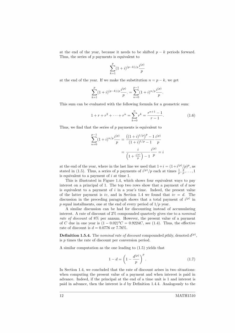
is equivalent to a payment of i at time 1.This is illustrated in Figure 1.4, which shows four equivalent ways to pay

interest on a principal of 1. The top two rows show that a payment of d nowis equivalent to a payment of i in a year’s time. Indeed, the present valueof the latter payment is iv, and in Section 1.4 we found that iv = d. Thediscussion in the preceding paragraph shows that a total payment of i(p) inp equal installments, one at the end of every period of 1/p year.

A similar discussion can be had for discounting instead of accumulatinginterest. A rate of discount of 2% compounded quarterly gives rise to a nominalrate of discount of 8% per annum. However, the present value of a paymentof C due in one year is (1 − 0.02)4C = 0.9224C, see (1.4). Thus, the effectiverate of discount is d = 0.0776 or 7.76%.

Definition 1.5.4. The nominal rate of discount compounded pthly, denoted d(p),is p times the rate of discount per conversion period.

A similar computation as the one leading to (1.5) yields that

1− d =(

1− d(p)

p

)p. (1.7)

In Section 1.4, we concluded that the rate of discount arises in two situations:when computing the present value of a payment and when interest is paid inadvance. Indeed, if the principal at the end of a time unit is 1 and interest ispaid in advance, then the interest is d by Definition 1.4.4. Analogously to the

12 MATH1510

t = 1t = 0

t = 1

i

t = 0

t = 1t = 0 1/p 2/p . . .

t = 1t = 0 1/p 2/p . . .

d

i(p)

p

d(p)

p

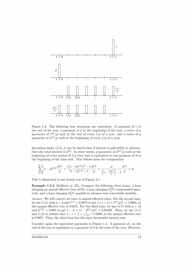
Figure 1.4: The following four situations are equivalent: A payment of i atthe end of the year, a payment of d at the beginning of the year, a series of ppayments of i(p)/p each at the end of every 1/p of a year, and a series of ppayments of d(p)/p each at the beginning of every 1/p of a year.

discussion under (1.5), it can be shown that if interest is paid pthly in advance,then the total interest is d(p). In other words, p payments of d(p)/p each at thebeginning of every period of 1/p time unit is equivalent to one payment of d atthe beginning of the time unit. This follows from the computation

p−1∑k=0

(1− d)k/pd(p)

p=

((1− d)1/p

)p − 1(1− d)1/p − 1

d(p)

p=

d(1− d(p)

p

)− 1

d(p)

p= d.

This is illustrated in the fourth row of Figure 4.1.

Example 1.5.5 (Kellison, p. 22). Compare the following three loans: a loancharging an annual effective rate of 9%, a loan charging 8 3

4% compounded quar-terly, and a loan charging 8 1

2% payable in advance and convertible monthly.

Answer. We will convert all rates to annual effective rates. For the second loan,we use (1.5) with p = 4 and i(4) = 0.0875 to get 1+i = (1+i(p)/p)p = 1.0904, sothe annual effective rate is 9.04%. For the third loan, we use (1.7) with p = 12and d(12) = 0.085 to get 1 − d = (1 − d(p)/p)p = 0.91823. Then, we use (1.1)and (1.3) to deduce that 1 + i = 1

v = 11−d = 1.0890, so the annual effective rate

is 8.90%. Thus, the third loan has the most favourable interest rate.

Consider again the equivalent payments in Figure 1.4. A payment of i at theend of the year is equivalent to a payment of d at the start of the year. However,

MATH1510 13

a payment made later is worth less than a payment made earlier. It follows thati has to be bigger than d. Similarly, the p payments of i(p)/p each in the thirdrow are done before the end of the year, with the exception of the last payment.Thus i(p) has to be smaller than i. Continuing this reasoning, we find that thediscount and interest rates are ordered as followed.

d < d(2) < d(3) < d(4) < · · · < i(4) < i(3) < i(2) < i.

Exercises

1. Express i(m) in terms of d(`), ` and m. Hence find i(12) when d(4) =0.057847.

2. (From the 2010 exam) How many days does it take for £1450 to accumu-late to £1500 under an interest rate of 4% p.a. convertible monthly?

3. (From the sample exam) Compute the nominal interest rate per annumpayable monthly that is equivalent to the simple interest rate of 7% p.a.over a period of three months.

14 MATH1510

Chapter 2

Annuities and loans

An annuity is a sequence of payments with fixed frequency. The term “annuity”originally referred to annual payments (hence the name), but it is now also usedfor payments with any frequency. Annuities appear in many situations; forinstance, interest payments on an investment can be considered as an annuity.An important application is the schedule of payments to pay off a loan.

The word “annuity” refers in everyday language usually to a life annuity. Alife annuity pays out an income at regular intervals until you die. Thus, thenumber of payments that a life annuity makes is not known. An annuity with afixed number of payments is called an annuity certain, while an annuity whosenumber of payments depend on some other event (such as a life annuity) is acontingent annuity. Valuing contingent annuities requires the use of probabil-ities and this will not be covered in this module. These notes only looks atannuities certain, which will be called “annuity” for short.

2.1 Annuities immediate

The analysis of annuities relies on the formula for geometric sums:

1 + r + r2 + · · ·+ rn =n∑k=0

rk =rn+1 − 1r − 1

. (2.1)

This formula appeared already in Section 1.5, where it was used to relate nom-inal interest rates to effective interest rates. In fact, the basic computations forannuities are similar to the one we did in Section 1.5. It is illustrated in thefollowing example.

Example 2.1.1. At the end of every year, you put £100 in a savings accountwhich pays 5% interest. You do this for eight years. How much do you have atthe end (just after your last payment)?

Answer. The first payment is done at the end of the first year and the lastpayment is done at the end of the eighth year. Thus, the first payment ac-cumulates interest for seven years, so it grows to (1 + 0.05)7 · 100 = 140.71pounds. The second payment accumulates interest for six years, so it grows to1.056 · 100 = 134.01 pounds. And so on, until the last payment which does not

MATH1510 15

t = 0 t = n. . .

sn

1 2

an

1

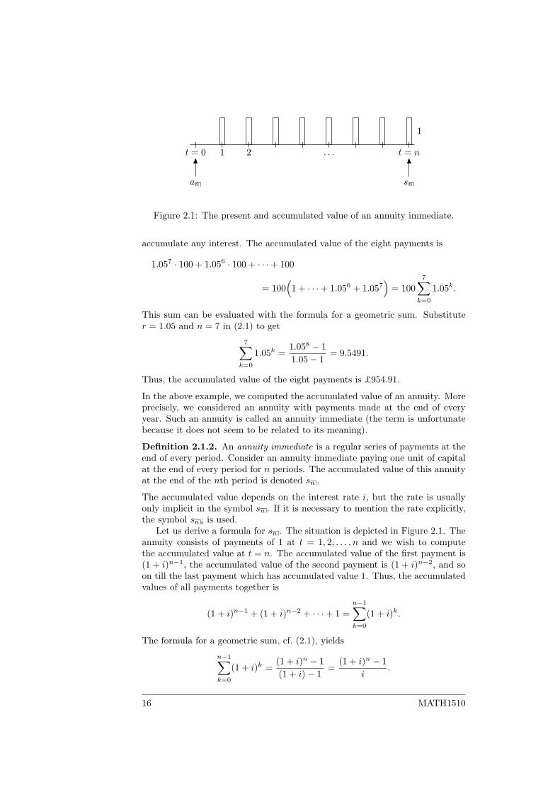
Figure 2.1: The present and accumulated value of an annuity immediate.

accumulate any interest. The accumulated value of the eight payments is

1.057 · 100 + 1.056 · 100 + · · ·+ 100

= 100(

1 + · · ·+ 1.056 + 1.057)

= 1007∑k=0

1.05k.

This sum can be evaluated with the formula for a geometric sum. Substituter = 1.05 and n = 7 in (2.1) to get

7∑k=0

1.05k =1.058 − 11.05− 1

= 9.5491.

Thus, the accumulated value of the eight payments is £954.91.

In the above example, we computed the accumulated value of an annuity. Moreprecisely, we considered an annuity with payments made at the end of everyyear. Such an annuity is called an annuity immediate (the term is unfortunatebecause it does not seem to be related to its meaning).

Definition 2.1.2. An annuity immediate is a regular series of payments at theend of every period. Consider an annuity immediate paying one unit of capitalat the end of every period for n periods. The accumulated value of this annuityat the end of the nth period is denoted sn .

The accumulated value depends on the interest rate i, but the rate is usuallyonly implicit in the symbol sn . If it is necessary to mention the rate explicitly,the symbol sn i is used.

Let us derive a formula for sn . The situation is depicted in Figure 2.1. Theannuity consists of payments of 1 at t = 1, 2, . . . , n and we wish to computethe accumulated value at t = n. The accumulated value of the first payment is(1 + i)n−1, the accumulated value of the second payment is (1 + i)n−2, and soon till the last payment which has accumulated value 1. Thus, the accumulatedvalues of all payments together is

(1 + i)n−1 + (1 + i)n−2 + · · ·+ 1 =n−1∑k=0

(1 + i)k.

The formula for a geometric sum, cf. (2.1), yields

n−1∑k=0

(1 + i)k =(1 + i)n − 1(1 + i)− 1

=(1 + i)n − 1

i.

16 MATH1510

We arrive at the following formula for the accumulated value of an annuityimmediate:

sn =(1 + i)n − 1

i. (2.2)

This formula is not valid if i = 0. In that case, there is no interest, so theaccumulated value of the annuities is just the sum of the payments: sn = n.

The accumulated value is the value of the annuity at t = n. We may alsobe interested in the value at t = 0, the present value of the annuity. This isdenoted by an , as shown in Figure 2.1.

Definition 2.1.3. Consider an annuity immediate paying one unit of capitalat the end of every period for n periods. The value of this annuity at the startof the first period is denoted an .

A formula for an can be derived as above. The first payment is made after ayear, so its present value is the discount factor v = 1

1+i . The present value ofthe second value is v2, and so on till the last payment which has a present valueof vn. Thus, the present value of all payments together is

v + v2 + · · ·+ vn = v(1 + v + ·+ vn−1) = v

n−1∑k=0

vk.

Now, use the formula for a geometric sum:

v

n−1∑k=0

vk = vvn − 1v − 1

=v

1− v(1− vn).

The fraction v1−v can be simplified if we use the relation v = 1

1+i :

v

1− v=

11+i

1− 11+i

=1

(1 + i)− 1=

1i.

By combining these results, we arrive at the following formula for the presentvalue of an annuity immediate:

an =1− vn

i. (2.3)

Similar to equation (2.2) for sn , the equation for an is not valid for i = 0, inwhich case an = n.

There is a simple relation between the present value an and the accumulatedvalue sn . They are value of the same sequence of payments, but evaluated atdifferent times: an is the value at t = 0 and sn is the value at t = n (seeFigure 2.1). Thus, an equals sn discounted by n years:

an = vnsn . (2.4)

This relation is easily checked. According to (2.2), the right-hand side evaluatesto

vnsn = vn(1 + i)n − 1

i=

(1+iv

)n − vni

=1− vn

i= an ,

MATH1510 17

where the last-but-one equality follows from v = 11+i and the last equality

from (2.3). This proves (2.4).One important application of annuities is the repayment of loans. This is

illustrated in the following example.

Example 2.1.4. A loan of e2500 at a rate of 6 12% is paid off in ten years,

by paying ten equal installments at the end of every year. How much is eachinstallment?

Answer. Suppose that each installment is x euros. Then the loan is paid off bya 10-year annuity immediate. The present value of this annuity is xa10 at 6 1

2%.We compute v = i

1+i = 0.938967 and

a10 =1− v10

i=

1− 0.93896710

0.065= 7.188830.

The present value should be equal to e2500, so the size of each installment isx = 2500/a10 = 347.7617 euros. Rounded to the nearest cent, this is e347.76.

Every installment in the above example is used to both pay interest and payback a part of the loan. This is studied in more detail in Section 2.6. Anotherpossibility is to only pay interest every year, and to pay back the principal atthe end. If the principal is one unit of capital which is borrowed for n years,then the borrower pays i at the end of every year and 1 at the end of the n years.The payments of i form an annuity with present value ian . The present valueof the payment of 1 at the end of n years is vn. These payments are equivalentto the payment of the one unit of capital borrowed at the start. Thus, we find

1 = ian + vn.

This gives another way to derive formula (2.3). Similarly, if we compare thepayments at t = n, we find

(1 + i)n = isn + 1,

and (2.2) follows.

Exercises

1. On 15 November in each of the years 1964 to 1979 inclusive an investordeposited £500 in a special bank savings account. On 15 November 1983the investor withdrew his savings. Given that over the entire period thebank used an annual interest rate of 7% for its special savings accounts,find the sum withdrawn by the investor.

2. A savings plan provides that in return for n annual premiums of £X(payable annually in advance), an investor will receive m annual paymentsof £Y , the first such payments being made one payments after paymentof the last premium.

(a) Show that the equation of value can be written as eitherY an+m − (X + Y )an = 0, or as (X + Y )sm −Xsn+m = 0.

18 MATH1510

t = 0 t = n. . .

sn

1 2

1

an

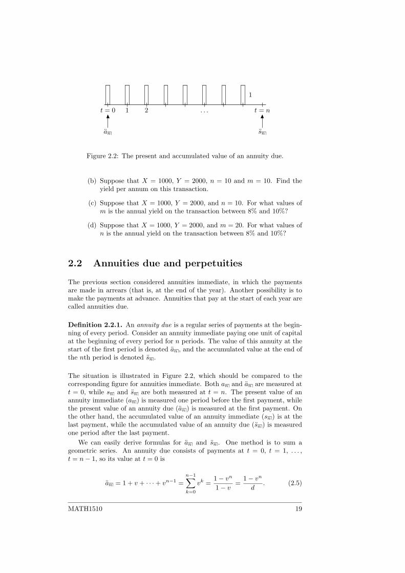
Figure 2.2: The present and accumulated value of an annuity due.

(b) Suppose that X = 1000, Y = 2000, n = 10 and m = 10. Find theyield per annum on this transaction.

(c) Suppose that X = 1000, Y = 2000, and n = 10. For what values ofm is the annual yield on the transaction between 8% and 10%?

(d) Suppose that X = 1000, Y = 2000, and m = 20. For what values ofn is the annual yield on the transaction between 8% and 10%?

2.2 Annuities due and perpetuities

The previous section considered annuities immediate, in which the paymentsare made in arrears (that is, at the end of the year). Another possibility is tomake the payments at advance. Annuities that pay at the start of each year arecalled annuities due.

Definition 2.2.1. An annuity due is a regular series of payments at the begin-ning of every period. Consider an annuity immediate paying one unit of capitalat the beginning of every period for n periods. The value of this annuity at thestart of the first period is denoted an , and the accumulated value at the end ofthe nth period is denoted sn .

The situation is illustrated in Figure 2.2, which should be compared to thecorresponding figure for annuities immediate. Both an and an are measured att = 0, while sn and sn are both measured at t = n. The present value of anannuity immediate (an ) is measured one period before the first payment, whilethe present value of an annuity due (an ) is measured at the first payment. Onthe other hand, the accumulated value of an annuity immediate (sn ) is at thelast payment, while the accumulated value of an annuity due (sn ) is measuredone period after the last payment.

We can easily derive formulas for an and sn . One method is to sum ageometric series. An annuity due consists of payments at t = 0, t = 1, . . . ,t = n− 1, so its value at t = 0 is

an = 1 + v + · · ·+ vn−1 =n−1∑k=0

vk =1− vn

1− v=

1− vn

d. (2.5)

MATH1510 19

The value at t = n is

sn = (1 + i)n + (1 + i)n−1 + · · ·+ (1 + i) =n∑k=1

(1 + i)k

= (1 + i)(1 + i)n − 1(1 + i)− 1

=1 + i

i

((1 + i)n − 1

)=

(1 + i)n − 1d

.

(2.6)

If we compare these formulas with the formulas for an and sn , given in (2.3)and (2.2), we see that they are identical except that the denominator is d insteadof i. In other words,

an =i

dan = (1 + i)an and sn =

i

dsn = (1 + i)sn .

There a simple explanation for this. An annuity due is an annuity immediatewith all payments shifted one time period in the past (compare Figures 2.1and 2.2). Thus, the value of an annuity due at t = 0 equals the value of anannuity immediate at t = 1. We know that an annuity immediate is worth anat t = 0, so its value at t = 1 is (1 + i)an and this has to equal an . Similarly,sn is not only the value of an annuity due at t = n but also the value of anannuity immediate at t = n + 1. Annuities immediate and annuities due referto the same sequence of payments evaluated at different times.

There is another relationship between annuities immediate and annuitiesdue. An annuity immediate over n years has payments at t = 1, . . . , t = n andan annuity due over n+ 1 years has payments at t = 0, t = 1, . . . , t = n. Thus,the difference is a single payment at t = 0. It follows that

an+1 = an + 1. (2.7)

Similarly, sn+1 is the value at t = n + 1 of a series of n + 1 payments attimes t = 1, . . . , n + 1, which is the same as the value at t = n of a series ofn+ 1 payments at t = 0, . . . , n. On the other hand, sn is the value at t = n ofa series of n payments at t = 0, . . . , n− 1. The difference is a single payment att = n, so

sn+1 = sn + 1. (2.8)

The relations (2.7) and (2.8) can be checked algebraically by substituting (2.2),(2.3), (2.5) and (2.6) in them.

There is an alternative method to derive the formulas for an and sn , anal-ogous to the discussion at the end of the previous section. Consider a loan ofone unit of capital over n years, and suppose that the borrower pays interest inadvance and repays the principal after n years. As discussed in Section 1.4, theinterest over one unit of capital is d if paid in advance, so the borrower paysan annuity due of size d over n years and a single payment of 1 after n years.These payments should be equivalent to the one unit of capital borrowed at thestart. By evaluating this equivalence at t = 0 and t = n, respectively, we findthat

1 = dan + vn and (1 + i)n = dsn + 1,

and the formulas (2.5) and (2.6) follow immediately.As a final example, we consider perpetuities, which are annuities continuing

perpetually. Consols, which are a kind of British government bonds, and certainpreferred stock can be modelled as perpetuities.

20 MATH1510

Definition 2.2.2. A perpetuity immediate is an annuity immediate contin-uing indefinitely. Its present value (one period before the first payment) isdenoted a∞ . A perpetuity due is an annuity due continuing indefinitely. Itspresent value (at the time of the first payment) is denoted a∞ .

There is no symbol for the accumulated value of a perpetuity, because it wouldbe infinite. It is not immediately obvious that the present value is finite, becauseit is the present value of an infinite sequence of payments. However, using theformula for the sum of an infinite geometric sequence (

∑∞k=0 r

k = 11−r ), we find

that

a∞ =∞∑k=0

vk =1

1− v=

1d

and

a∞ =∞∑k=1

vk = v

∞∑k=0

vk =v

1− v=

1i.

Alternatively, we can use a∞ = limn→∞ an and a∞ = limn→∞ an in combina-tion with the formulas for an and an . This method gives the same result.

Example 2.2.3. You want to endow a fund which pays out a scholarship of£1000 every year in perpetuity. The first scholarship will be paid out in fiveyears’ time. Assuming an interest rate of 7%, how much do you need to payinto the fund?

Answer. The fund makes payments of £1000 at t = 5, 6, 7, . . ., and we wish tocompute the present value of these payments at t = 0. These payments form aperpetuity, so the value at t = 5 is a∞ . We need to discount by five years tofind the value at t = 0:

v5a∞ =v5

d=

0.9345795

0.0654206= 10.89850.

Thus, the fund should be set up with a contribution of £10898.50.Alternatively, imagine that the fund would be making annual payments

starting immediately. Then the present value at t = 0 would be 1000a∞ .However, we added imaginary payments at t = 0, 1, 2, 3, 4; the value at t = 0 ofthese imaginary payments is 1000a5 . Thus, the value at t = 0 of the paymentsat t = 5, 6, 7, . . . is

1000a∞ − 1000a5 = 1000 · 1d− 1000 · 1− v5

d= 15285.71− 4387.21 = 10898.50,

as we found before. This alternative method is not faster in this example, butit illustrates a reasoning which is useful in many situations.

An annuity which starts paying in the future is called a deferred annuity. Theperpetuity in the above example has its first payment in five years’ time, soit can be considered as a perpetuity due deferred by five years. The actuarialsymbol for the present value of such a perpetuity is 5|a∞ . Alternatively, we canconsider the example as a perpetuity immediate deferred by four years, whosepresent value is denoted by 4|a∞ . Generally, the present value of an annuitiesover n years deferred by m years is given

m|an = vman and m|an = vman .

MATH1510 21

Exercises

1. A loan of £2400 is to be repaid by 20 equal annual instalments. The rateof interest for the transaction is 10% per annum. Fiund the amount ofeach annual repayment, assuming that payments are made (a) in arrearand (b) in advance.

2.3 Unknown interest rate

In Sections 2.1 and 2.2 we derived the present and accumulated values of annu-ities with given period n and interest rate i. In Section 2.7, we studied how tofind n. The topic of the current section is the determination of the rate i.

Example 2.3.1 (McCutcheon & Scott, p. 48). A loan of £5000 is repaid by15 annual payments of £500, with the first payment due in a year. What is theinterest rate?

Answer. The repayments form an annuity. The value of this annuity at thetime of the loan, which is one year before the first payment, is 500a15 . Thishas to equal the principal, so we have to solve 500a15 = 5000 or a15 = 0.1.Formula (2.3) for an yields

a15 =1− v15

i=

1i

(1−

(1

1 + i

)15),

so the equation that we have to solve is

1i

(1−

(1

1 + i

)15)

= 10. (2.9)

The solution of this equation is i = 0.055565, so the rate is 5.56%.

The above example is formulated in terms of a loan, but it can also be formulatedfrom the view of the lender. The lender pays £5000 and gets 15 annual paymentsof £500 in return. The interest rate implied by the transaction is called the yieldor the (internal) rate of return of the transaction. It is an important conceptwhen analysing possible investments. Obviously, an investor wants to get highyield on his investment. We will return to this in Chapter 3.

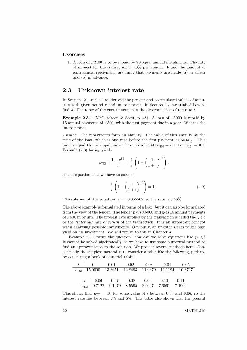
Example 2.3.1 raises the question: how can we solve equations like (2.9)?It cannot be solved algebraically, so we have to use some numerical method tofind an approximation to the solution. We present several methods here. Con-ceptually the simplest method is to consider a table like the following, perhapsby consulting a book of actuarial tables.

i 0 0.01 0.02 0.03 0.04 0.05a15 15.0000 13.8651 12.8493 11.9379 11.1184 10.3797

i 0.06 0.07 0.08 0.09 0.10 0.11a15 9.7122 9.1079 8.5595 8.0607 7.6061 7.1909

This shows that a15 = 10 for some value of i between 0.05 and 0.06, so theinterest rate lies between 5% and 6%. The table also shows that the present

22 MATH1510

an

14

12

10

8

0 0.04 0.08i

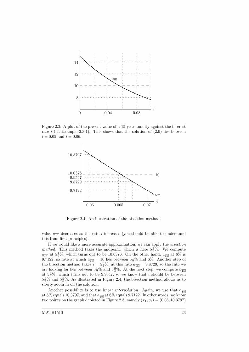
Figure 2.3: A plot of the present value of a 15-year annuity against the interestrate i (cf. Example 2.3.1). This shows that the solution of (2.9) lies betweeni = 0.05 and i = 0.06.

i

an

0.070.0650.06

9.9547

9.7122

10.3797

10.0376

9.8729

10

Figure 2.4: An illustration of the bisection method.

value a15 decreases as the rate i increases (you should be able to understandthis from first principles).

If we would like a more accurate approximation, we can apply the bisectionmethod. This method takes the midpoint, which is here 5 1

2%. We computea15 at 5 1

2%, which turns out to be 10.0376. On the other hand, a15 at 6% is9.7122, so rate at which a15 = 10 lies between 5 1

2% and 6%. Another step ofthe bisection method takes i = 5 3

4%; at this rate a15 = 9.8729, so the rate weare looking for lies between 5 1

2% and 5 34%. At the next step, we compute a15

at 5 58%, which turns out to be 9.9547, so we know that i should be between

5 12% and 5 5

8%. As illustrated in Figure 2.4, the bisection method allows us toslowly zoom in on the solution.

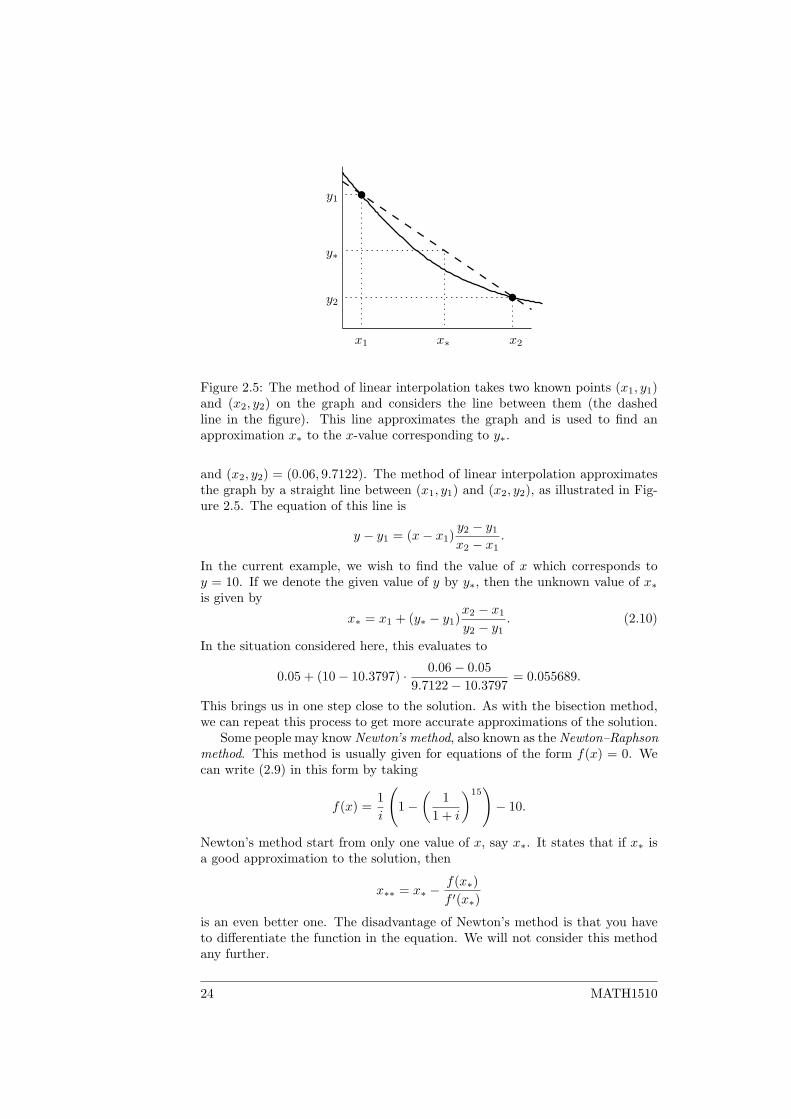
Another possibility is to use linear interpolation. Again, we use that a15

at 5% equals 10.3797, and that a15 at 6% equals 9.7122. In other words, we knowtwo points on the graph depicted in Figure 2.3, namely (x1, y1) = (0.05, 10.3797)

MATH1510 23

x2x∗x1

y2

y1

y∗

Figure 2.5: The method of linear interpolation takes two known points (x1, y1)and (x2, y2) on the graph and considers the line between them (the dashedline in the figure). This line approximates the graph and is used to find anapproximation x∗ to the x-value corresponding to y∗.

and (x2, y2) = (0.06, 9.7122). The method of linear interpolation approximatesthe graph by a straight line between (x1, y1) and (x2, y2), as illustrated in Fig-ure 2.5. The equation of this line is

y − y1 = (x− x1)y2 − y1x2 − x1

.

In the current example, we wish to find the value of x which corresponds toy = 10. If we denote the given value of y by y∗, then the unknown value of x∗is given by

x∗ = x1 + (y∗ − y1)x2 − x1

y2 − y1. (2.10)

In the situation considered here, this evaluates to

0.05 + (10− 10.3797) · 0.06− 0.059.7122− 10.3797

= 0.055689.

This brings us in one step close to the solution. As with the bisection method,we can repeat this process to get more accurate approximations of the solution.

Some people may know Newton’s method, also known as the Newton–Raphsonmethod. This method is usually given for equations of the form f(x) = 0. Wecan write (2.9) in this form by taking

f(x) =1i

(1−

(1

1 + i

)15)− 10.

Newton’s method start from only one value of x, say x∗. It states that if x∗ isa good approximation to the solution, then

x∗∗ = x∗ −f(x∗)f ′(x∗)

is an even better one. The disadvantage of Newton’s method is that you haveto differentiate the function in the equation. We will not consider this methodany further.

24 MATH1510

All these methods are quite cumbersome to use by hand, so people commonlyuse some kind of machine to solve equations like these. Some graphical calcu-lators allow you to solve equations numerically. Financial calculators generallyhave an option to find the interest rate of an annuity, given the number of pay-ments, the size of every payment, and the present or accumulated value. Thereare also computer programs that can assist you with these computations. Forexample, in Excel the command RATE(15,500,-5000) computes the unknownrate in Example 2.3.1.

Exercises

1. A borrower agrees to repay a loan of £3000 by 15 annual repayments of£500, the first repayment being due after five years. Find the annual yieldfor this transaction.

2. (From the sample exam) A loan of £50,000 is repaid by annual paymentsof £4000 in arrear over a period of 20 years. Write down the equation ofvalue and use linear interpolation with trial values of i = 0.04 and i = 0.07to approximate the effective rate of interest per annum.

2.4 Annuities payable monthly, etc.

Up to now all annuities involved annual payments. However, other frequenciescommonly arise in practice. The same theory as developed above apply toannuities with other frequencies.

Example 2.1.1 shows that the accumulated value of a sequence of eight an-nual payments of £100 at the time of the last payment is £954.91, if the rate ofinterest is 5% per annum. The result remains valid if we change the time unit.The same computation shows that the accumulated value of a sequence of eightmonthly payments of £100 at the time of the last payment is £954.91, if therate of interest is 5% per month.

Interest rates per month are not used very often. As explained in Section 1.5,a rate of 5% per month corresponds to a nominal rate i(12) of 60% per yearpayable monthly (computed as 60 = 5× 12). It also corresponds to an effectiverate i of 79.59% per year, because (1.05)12 = 1.7959. Thus, the accumulatedvalue of a sequence of eight monthly payments of £100 at the time of the lastpayment is £954.91, if the (effective) rate of interest is 79.59% p.a.

The preceding two paragraphs illustrate the basic idea of this section. Theremainder elaborates on this and gives some definitions.

Definition 2.4.1. An annuity immediate payable pthly is a regular series ofpayments at the end of every period of 1/p time unit. Consider such an annuitylasting for n time units (so there are np payments), where every payment is1/p unit of capital (so the total payment is n units). The present value of thisannuity at the start of the first period is denoted a

(p)n , and the accumulated

value at the end of the npth period is denoted s(p)n .

The present and accumulated value of an annuity immediate payable pthly onthe basis of an interest rate i per time unit can be calculated using several

MATH1510 25

methods. Three methods will be presented here. All these methods use thenominal interest rate i(p) payable pthly, which is related to i by (1.5):

1 + i =(

1 +i(p)

p

)p.

The first method is the one used at the start of the section, in which a new timeunit is introduced which equals the time between two payments (i.e., 1/p oldtime units). The rate i per old time unit corresponds to a rate of j = i(p)/p pernew time unit, and the annuity payable pthly becomes a standard annuity overnp (new) time units, with one payment of 1/p per (new) time unit. The futurevalue of this annuity is 1

psnp j , which can be evaluated using (2.2):

s(p)n i = 1

psnp j =(1 + j)np − 1

jp=

(1 + i(p)

p

)np − 1

i(p)=

(1 + i)n − 1i(p)

.

To compute the present value of the annuity over np time units, with one pay-ment of 1/p per time unit, use (2.3) while bearing in mind that the discountfactor in new time units is 1/(1 + j):

a(p)n i = 1

panp j =1−

(1

1+j )np

jp=

1−(1 + i(p)

p

)−npi(p)

=1− (1 + i)−n

i(p)=

1− vn

i(p).

The second method computes the present and accumulated value of annuitiespayable pthly from first principles using formula (2.1) for the sum of a geometricsequence. This is the same method used to derive formulas (2.2) and (2.3). Thesymbol a(p)

n denotes the present value at t = 0 of np payments of 1/p each. Thefirst payment is at time t = 1/p, so its present value is (1/p) · v1/p; the secondpayment is at time t = 2/p, so its present value is (1/p) · v2/p; and so on till thelast payment which is at time t = n, so its present value is (1/p) · vn. The sumof the present values is:

a(p)n =

1p

(v1/p + v2/p + · · ·+ vn−

1p + vn

)=

1p

np∑k=1

vk/p

=v1/p

p· 1− (v1/p)np

1− v1/p=

1p· 1− vn

(1 + i)1/p − 1=

1− vn

i(p).

Similarly, the accumulated value is computed as

s(p)n =

1p

((1 + i)n−

1p + (1 + i)n−

2p + · · ·+ (1 + i)1/p + 1

)=

1p

np−1∑k=0

(1 + i)k/p =1p· ((1 + i)1/p)np − 1

(1 + i)− 1=

(1 + i)n − 1i(p)

.

The third method compares an annuity payable pthly to an annuity payableannually over the same period. In one year, an annuity payable pthly consistsof p payments (at the end of every period of 1/p year) and an annuity payableannually consists of one payment at the end of the year. If p payments are i(p)/peach and the annual payment is i, then these payments are equivalent, as was

26 MATH1510

found in Section 1.5 (see Figure 4.1). Thus, an annuity with pthly paymentsof i(p)/p is equivalent to an annuity with annual payments of i, so their presentand accumulated values are the same:

ian = i(p)a(p)n and isn = i(p)s

(p)n .

All three methods leads to the same conclusion:

a(p)n =

1− vn

i(p)and s

(p)n =

(1 + i)n − 1i(p)

. (2.11)

The formulas for annuities payable pthly are the same as the formulas for stan-dard annuities (that is, annuities payable annually), except that the formulas forannuities payable pthly have the nominal interest rate i(p) in the denominatorinstead of i.

A similar story holds for annuities due. An annuity due payable pthly is asequence of payments at t = 0, 1/p, . . . , n−(1/p), whereas an annuity immediatepayable pthly is a sequence of payments at t = 1/p, 2/p, . . . , n. Thus, theyrepresent the same sequence of payments, but shifted by one period of 1/ptime unit. The present value of an annuity due payable pthly at t = 0 isdenoted by a

(p)n , and the accumulated value at t = n is denoted by s

(p)n . The

corresponding expressions are

a(p)n =

1− vn

d(p)and s

(p)n =

(1 + i)n − 1d(p)

. (2.12)

The difference with the formulas (2.11) for annuities immediate is again only inthe denominator: i(p) is replaced by d(p).

The above discussion tacitly assumed that p is an integer, but in fact theresults are also valid for fractional values of p. This is illustrated in the followingexample.

Example 2.4.2. Consider an annuity of payments of £1000 at the end of everysecond year. What is the present value of this annuity if it runs for ten yearsand the interest rate is 7%?

Answer. The present value can be found from first principles by summing ageometric sequence. We have i = 0.07 so v = 1/1.07 = 0.934579, so the presentvalue is

1000v2 + 1000v4 + 1000v6 + 1000v8 + 1000v10

= 10005∑k=1

v2k = 1000v2 · 1− (v2)5

1− v2= 3393.03 pounds.

Alternatively, we can use (2.11) with p = 1/2, because there is one payment pertwo years. We compute i(1/2) from (1.5),

1 + i =(

1 +i(1/2)

1/2

)1/2

=⇒ i(1/2) =12

((1 + i)2 − 1

)= 0.07245,

and thus

a(1/2)

10=

1− v10

i(1/2)= 6.786069.

MATH1510 27

Remember that a(p)n is the present value of an annuity paying 1/p units of capital

every 1/p years for a period of n years, so a(1/2)

10= 6.786069 is the present value

of an annuity paying two units of capital every two years for a period of 10 years.Thus, the present value of the annuity in the question is 500·6.786069 = 3393.03pounds. This is the same as we found from first principles.

Exercises

1. (From the 2010 exam)

(a) A savings plan requires you to make payments of £250 each at theend of every month for a year. The bank will then make six equalmonthly payments to you, with its first payment due one month afterthe last payment you make to the bank. Compute the size of eachmonthly payment made by the bank, assuming a nominal interestrate of 4% p.a. payable monthly.

(b) The situation is the same as in question (a): you make paymentsof £250 each at the end of every month for a year, and the rate is4% p.a. payable monthly. However, now the bank will make equalannual payments to you in perpetuity, with the first payment duethree years after the last payment you make to the bank. Computethe size of the annual payments.

2. (From the sample exam) A 20-year loan of £50,000 is repaid as follows.The borrower pays only interest on the loan, annually in arrear at a rateof 5.5% per annum. The borrower will take out a separate savings pol-icy which involves making monthly payments in advance such that theproceeds will be sufficient to repay the loan at the end of its term. Thepayments into the savings policy accumulate at a rate of interest of 4%per annum effective.

Compute the monthly payments into the savings account which ensuresthat it contains £50,000 after 20 years, and write down the equation ofvalue for the effective rate of interest on the loan if it is repaid using thisarrangement.

3. (From the CT1 exam, Sept ’08) A bank offers two repayment alternativesfor a loan that is to be repaid over ten years. The first requires theborrower to pay £1,200 per annum quarterly in advance and the secondrequires the borrower to make payments at an annual rate of £1,260 everysecond year in arrears. Determine which terms would provide the best dealfor the borrower at a rate of interest of 4% per annum effective.

2.5 Varying annuities

The annuities studied in the preceding sections are all level annuities, meaningthat all payments are equal. This section studies annuities in which the size ofthe payments changes. In simple cases, these can be studied by splitting thevarying annuities in a sum of level annuities, as the following example shows.

28 MATH1510

Example 2.5.1. An annuity pays e50 at the end of every month for two years,and e60 at the end of every month for the next three years. Compute thepresent value of this annuity on the basis of an interest rate of 7% p.a.

Answer. This annuity can be considered as the sum of two annuities: one of e50per month running for the first two years, and one of e60 per month runningfor the next three years. The present value of the first annuity is 600a(12)

2euros

(remember that a(12)n is the present value of an annuity paying 1/12 at the end

of every month). The value of the second annuity one month before its firstpayment is 720a(12)

3, which we need to discount by two years. Thus, the present

value of the annuity in the question is

600a(12)

2+ 720v2a

(12)

3= 600 · 1− v2

i(12)+ 720v2 · 1− v3

i(12).

The interest rate is i = 0.07, so the discount factor is v = 1/1.07 = 0.934579and the nominal interest rate is i(12) = 12(1.071/12 − 1) = 0.0678497, so

600 · 1− v2

i(12)+ 720v2 · 1− v3

i(12)= 1119.19 + 1702.67 = 2821.86.

Thus, the present value of the annuity in the question is e2821.86.Alternatively, the annuity can be considered as the difference between an

annuity of e60 per month running for five years and an annuity of e10 permonth running for the first two years. This argument shows that the presentvalue of the annuity in the question is

720a(12)

5− 120a(12)

2= 3045.70− 223.84 = 2821.86.

Unsurprisingly, this is the same answer as we found before.

More complicated examples of varying annuities require a return to first prin-ciples. Let us consider a varying annuity immediate running over n time units,and denote the amount paid at the end of the kth time unit by Pk. The presentvalue of this annuity, one time unit before the first payment, is given by

n∑k=1

Pkvk,

and its accumulated value at the time of the last payment is given by

n∑k=1

Pk(1 + i)n−i.

For a level annuity, all the Pk are equal, and we arrive at the formulas for anand sn . The next example considers an annuity whose payments increase geo-metrically.

Example 2.5.2. An annuity immediate pays £1000 at the end of the first year.The payment increases by 3% per year to compensate for inflation. What is thepresent value of this annuity on the basis of a rate of 7%, if it runs for 20 years?

MATH1510 29

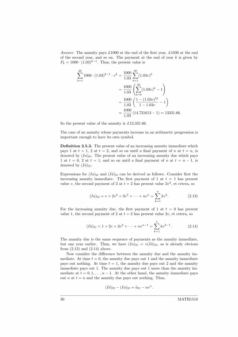
Answer. The annuity pays £1000 at the end of the first year, £1030 at the endof the second year, and so on. The payment at the end of year k is given byPk = 1000 · (1.03)k−1. Thus, the present value is

20∑k=1

1000 · (1.03)k−1 · vk =10001.03

20∑k=1

(1.03v)k

=10001.03

(20∑k=0

(1.03v)k − 1

)

=10001.03

(1− (1.03v)21

1− 1.03v− 1)

=10001.03

(14.731613− 1) = 13331.66.

So the present value of the annuity is £13,331.66.

The case of an annuity whose payments increase in an arithmetic progression isimportant enough to have its own symbol.

Definition 2.5.3. The present value of an increasing annuity immediate whichpays 1 at t = 1, 2 at t = 2, and so on until a final payment of n at t = n, isdenoted by (Ia)n . The present value of an increasing annuity due which pays1 at t = 0, 2 at t = 1, and so on until a final payment of n at t = n − 1, isdenoted by (Ia)n .

Expressions for (Ia)n and (Ia)n can be derived as follows. Consider first theincreasing annuity immediate. The first payment of 1 at t = 1 has presentvalue v, the second payment of 2 at t = 2 has present value 2v2, et cetera, so

(Ia)n = v + 2v2 + 3v3 + · · ·+ nvn =n∑k=1

kvk. (2.13)

For the increasing annuity due, the first payment of 1 at t = 0 has presentvalue 1, the second payment of 2 at t = 2 has present value 2v, et cetera, so

(Ia)n = 1 + 2v + 3v2 + · · ·+ nvn−1 =n∑k=1

kvk−1. (2.14)

The annuity due is the same sequence of payments as the annuity immediate,but one year earlier. Thus, we have (Ia)n = v(Ia)n , as is already obviousfrom (2.13) and (2.14) above.

Now consider the difference between the annuity due and the annuity im-mediate. At time t = 0, the annuity due pays out 1 and the annuity immediatepays out nothing. At time t = 1, the annuity due pays out 2 and the annuityimmediate pays out 1. The annuity due pays out 1 more than the annuity im-mediate at t = 0, 1, . . . , n − 1. At the other hand, the annuity immediate paysout n at t = n and the annuity due pays out nothing. Thus,

(Ia)n − (Ia)n = an − nvn.

30 MATH1510

This can also be found by subtracting (2.13) from (2.14). Now use that (Ia)n =v(Ia)n , as we found above:

1v

(Ia)n − (Ia)n = an − nvn =⇒ (Ia)n =an − nvn

1v − 1

=an − nvn

i.

This can be written as an = i(Ia)n +nvn, an equation with an interesting (butperhaps challenging) interpretation. Consider a transaction, in which one unitof capital is lent every year. The interest is i in the first year, 2i in the secondyear, and so on. At the end of n years, the amount borrowed is n, which is thenpaid back. The equation an = i(Ia)n + nvn expresses that the payments doneby the lender are equivalent to the payments by the borrower.

The formula for (Ia)n can be used to find the value of annuities with pay-ments in an arithmetic progression. For instance, consider an annuity paying£1000 at the end of the first year, £950 at the end of the second year, £900 atthe end of the third year, and so on, with the payment decreasing by £50 everyear. The last payment is £500 at the end of the eleventh year. The presentvalue of this annuity is 1050a11 − 50(Ia)11 .

Exercises

1. An annuity is payable in arrear for 20 years. The first payment is ofamount £8000 and the amount of each subsequence payment decreases by£300 each year. Find the present value of the annuity on the basis of aninterest rate of 5% per annum.

2. An annuity is payable half-yearly for six years, the first half-yearly pay-ment of amount £1800 being due after two years. The amount of sub-sequent payments decreases by £30 every half-year. On the basis of aninterest rate of 5% per half-year, find the present value of the annuity.

3. ((From the 2010 exam) An annuity pays out on 1 January in every year,from 1 January 2011 up to (and including) 1 January 2030. The annuitypays £1000 in odd years (2011, 2013, 2015, etc.) and £2000 in even years(2012, 2014, 2016, etc.). Compute the present value of this annuity on 1January 2011 on the basis on an interest rate of 6% p.a.

4. (From the sample exam) An individual wishes to receive an annuity whichis payable monthly in arrears for 15 years. The annuity is to commencein exactly 10 years at an initial rate of £12,000 per annum. The pay-ments increase at each anniversary by 3% per annum (so the first twelvepayments are £1000, the next twelve payments are £1030, and so on).Compute the amount needed to purchase this annuity now assuming aninterest rate of 6% per annum effective.

5. (From the CT1 exam, Sept ’09) A member of a pensions savings schemeinvests £1,200 per annum in monthly instalments, in advance, for 20 yearsfrom his 25th birthday. From the age of 45, the member increases his in-vestment to £2,400 per annum. At each birthday thereafter the annualrate of investment is further increased by £100 per annum. The invest-ments continue to be made monthly in advance for 20 years until theindividuals 65th birthday.

MATH1510 31

(a) Calculate the accumulation of the investment at the age of 65 usinga rate of interest of 6% per annum effective.

(b) At the age of 65, the scheme member uses his accumulated investmentto purchase an annuity with a term of 20 years to be paid half-yearlyin arrear. At this time the interest rate is 5% per annum convertiblehalf-yearly. Calculate the annual rate of payment of the annuity.

2.6 Loans

Example 2.1.4 considered the repayment of a loan by a level annuity. Therepayment of loans is an important application of annuities, which is studiedfurther in this section.

Example 2.6.1 (Continuation of Example 2.1.4). We computed that a loanof e2500 at 6 1

2% interest can be repaid by ten installments of e347.76, eachbeing paid at the end of the year. What is the remaining balance of the loanafter six years?

Answer. There are two methods to handle questions like this. The first methodconsiders the payments in the first six years. This is called the retrospectivemethod, because it looks back to payments already made. The second methodconsiders the payments in the last four years. This is called the prospectivemethod, because it looks forward to payments that have not been made yet.Obviously, both methods should give the same answer, and you should pick themethod that seems more convenient.

The retrospective method uses that the remaining balance is the value ofthe original loan after six years minus the accumulated value of the paymentsthat have already been made. The borrower has made six payments of e347.76each at the end of the year. The accumulated value of these payments is

347.76 · s6 = 347.76 · 7.063728 = 2456.48.

The value of the loan after six years is

2500 · (1 + i)6 = 2500 · 1.459142 = 3647.86,

so the remaining balance of the loan is 3647.86− 2456.48 = 1191.38 euros.The prospective method uses that the remaining balance equals the present

value of the remaining payments. The borrower still has to make four paymentsof e347.76. We need the present value of these payments six years after the startof the loan. This is one year before the first of the four remaining payments isdue, so the present value of the four remaining payments is

347.76 · a4 = 347.76 · 3.425799 = 1191.36

euros. Thus, the remaining balance of the loan after six years is e1191.36.The results found by the retrospective and prospective methods differ by

two cents. The difference is caused because at the end of Example 2.1.4, thevalue of 347.7617 . . . was rounded to 347.76. The prospective and retrospectivemethod would have given the same result if we had used the exact value.

32 MATH1510

Interest Principal OutstandingYear Payment paid repaid balance

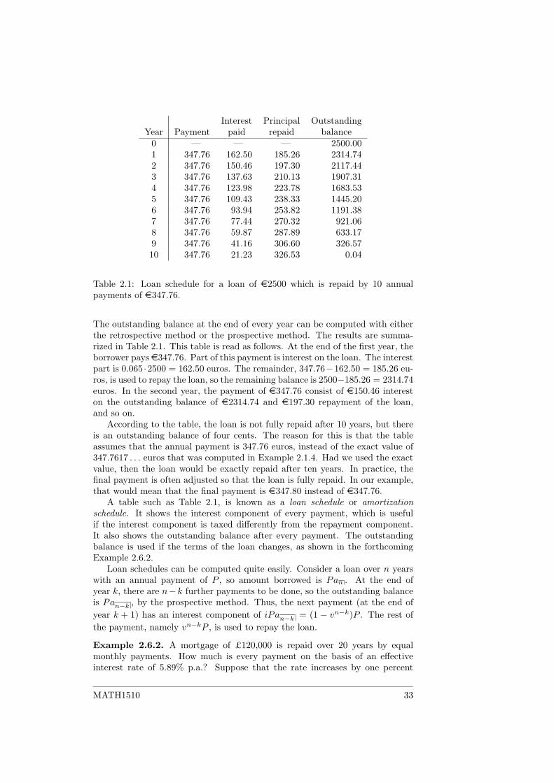
0 — — — 2500.001 347.76 162.50 185.26 2314.742 347.76 150.46 197.30 2117.443 347.76 137.63 210.13 1907.314 347.76 123.98 223.78 1683.535 347.76 109.43 238.33 1445.206 347.76 93.94 253.82 1191.387 347.76 77.44 270.32 921.068 347.76 59.87 287.89 633.179 347.76 41.16 306.60 326.5710 347.76 21.23 326.53 0.04

Table 2.1: Loan schedule for a loan of e2500 which is repaid by 10 annualpayments of e347.76.

The outstanding balance at the end of every year can be computed with eitherthe retrospective method or the prospective method. The results are summa-rized in Table 2.1. This table is read as follows. At the end of the first year, theborrower pays e347.76. Part of this payment is interest on the loan. The interestpart is 0.065 ·2500 = 162.50 euros. The remainder, 347.76−162.50 = 185.26 eu-ros, is used to repay the loan, so the remaining balance is 2500−185.26 = 2314.74euros. In the second year, the payment of e347.76 consist of e150.46 intereston the outstanding balance of e2314.74 and e197.30 repayment of the loan,and so on.

According to the table, the loan is not fully repaid after 10 years, but thereis an outstanding balance of four cents. The reason for this is that the tableassumes that the annual payment is 347.76 euros, instead of the exact value of347.7617 . . . euros that was computed in Example 2.1.4. Had we used the exactvalue, then the loan would be exactly repaid after ten years. In practice, thefinal payment is often adjusted so that the loan is fully repaid. In our example,that would mean that the final payment is e347.80 instead of e347.76.

A table such as Table 2.1, is known as a loan schedule or amortizationschedule. It shows the interest component of every payment, which is usefulif the interest component is taxed differently from the repayment component.It also shows the outstanding balance after every payment. The outstandingbalance is used if the terms of the loan changes, as shown in the forthcomingExample 2.6.2.

Loan schedules can be computed quite easily. Consider a loan over n yearswith an annual payment of P , so amount borrowed is Pan . At the end ofyear k, there are n−k further payments to be done, so the outstanding balanceis Pan−k , by the prospective method. Thus, the next payment (at the end ofyear k + 1) has an interest component of iPan−k = (1 − vn−k)P . The rest ofthe payment, namely vn−kP , is used to repay the loan.

Example 2.6.2. A mortgage of £120,000 is repaid over 20 years by equalmonthly payments. How much is every payment on the basis of an effectiveinterest rate of 5.89% p.a.? Suppose that the rate increases by one percent

MATH1510 33

point after eleven years. Compute the revised monthly payment.

Answer. The rate of i = 0.0589 corresponds to a nominal rate payable monthlyof

i(12) = 12(

(1 + i)1/12 − 1)

= 0.05736732.

If every monthly payment is 1/12, then the present value of all the monthlypayments is

a(12)

20=

1− v20

i(12)=

1− 1.0589−20

0.05736732= 11.882249.

Thus, the monthly repayment required to pay off the mortgage of £120,000 is

120000

a(12)

20

· 112

= 841.59 pounds.

Now consider the situation after eleven years. There are nine years of paymentsremaining. The present value of these payments is

841.59 · 12 · a(12)

9= 841.49 · 11 · 7.016967 = 70864.91

pounds, so by the prospective method the outstanding balance is £70,864.91.It may seem surprising that less than half the loan is repaid in the first elevenyears, but at the start of the loan most of the payments are used to pay theinterest. The bulk of the loan is repaid in the second half.

To compute the revised monthly payment after the rate increase, we computethe revised nominal rate as

i(12) = 12(

(1.0689)1/12 − 1)

= 0.06681541.

There are nine years of monthly payments left, in which £70,864.91 needs to berepaid, so the revised monthly payment is

70864.91

a(12)

9

· 112

=70864.916.750054

· 112

= 874.87.

Thus, the rate increase causes the monthly payment to be increased from£841.59 to £874.87.

Exercises

1. (From the 2010 exam) A four-year loan of £5000 is repaid by equal annualpayments at the end of each year. Compute the annual payment on thebasis of an interest rate of 6% p.a. and draw up a loan schedule, showingthe interest component of every payment and the outstanding balance.

2. (From the CT1 exam, April ’08) A mortgage company offers the followingtwo deals to customers for twenty-five year mortgages.

(a) A mortgage of £100,000 is offered with level repayments of £7,095.25made annually in arrear. There are no arrangement or exit fees.

34 MATH1510

(b) A mortgage of £100,000 is offered whereby a monthly payment inadvance is calculated such that the customer pays an effective rateof return of 4% per annum ignoring arrangement and exit fees. Inaddition the customer also has to pay an arrangement fee of £6,000at the beginning of the mortgage and an exit fee of £5,000 at the endof the twenty-five year term of the mortgage.

Compare the annual effective rates of return paid by customers on the twoproducts.

3. (From the CT1 exam, April ’09) A loan is to be repaid by an annuitypayable annually in arrear. The annuity starts at a rate of £300 perannum and increases each year by £30 per annum. The annuity is to bepaid for 20 years. Repayments are calculated using a rate of interest of7% per annum effective.

Calculate:

(a) The amount of the loan.

(b) The capital outstanding immediately after the 5th payment has beenmade.

(c) The capital and interest components of the final payment.

2.7 Annuities over non-integer periods

It is fairly easy to compute the number n of payments of an annuity givenits present or accumulated value, as the following example shows. However, theresult is usually not an integer. This section explains how to interpret fractionalperiods.

Example 2.7.1. A loan of $10000 is repaid by annual payments of $1000 eachat the end of the year. How long does it take to repay the loan on the basis ofan interest rate of 6% p.a.?

Answer. The annual payments form an annuity immediate. Its present valueis 1000an . This should equal the amount borrowed, so we have to solve an = 10for n. Using (2.3), we find:

an = 10 =⇒ 1− vn

i= 10

=⇒ vn = 1− 10i

=⇒ n =log(1− 10i)

log(v)= 15.725,

so the solution is n = 15.725.

How should we to interpret the result n = 15.725? What does it mean tohave an annuity over 15.725 years? One possibility is that the borrower shouldmake 15 payments of $1000 at t = 1, . . . , 15, and one final payment at timet = 15.725 (after 15 years and 265 days). The present value of the 15 paymentsof $1000 is 1000a15 = 9712.25 dollars, so after these payments $287.75 of theloan is still outstanding. Thus, the final payment at t = 15.725 should be

MATH1510 35

(1 + i)15.725 · 287.75 = 718.38 dollars. The loan is repaid by 15 paymentsof $1000, paid annually in arrears, and a final payment of $718.38, paid after15 years and 265 days.

This interpretation is possible but not used very often in practice, becauseit is more convenient for both parties to have all payments at regular times.Usually, either the payment at t = 15 is increased so that the entire loan isrepaid at that time, or a payment is added at t = 16 to repay the remainder ofthe loan. In the first case, the borrower has to pay (1 + i)15 · 287.75 = 689.61dollars extra at t = 15, so the loan is repaid by 14 payments of $1000 att = 1, . . . , 14 and a final payment of $1689.61. The payment of $1689.61 at theend is called the balloon payment. In the second case, the borrower has to makean additional payment of (1 + i)16 · 287.75 = 730.99 dollars at t = 16, so theloan is repaid by 15 payments of $1000 at t = 1, . . . , 15 and a final paymentof $730.99 at t = 16. The payment of $730.99 at the end is called the droppayment. In conclusion, we found three possible interpretations of the annuityover 15.725 years, that resulted in the situation of Example 2.7.1:

• The borrower pays $1000 at t = 1, . . . , 14 and $1689.61 at t = 15.

• The borrower pays $1000 at t = 1, . . . , 15 and $718.38 at t = 15.725.

• The borrower pays $1000 at t = 1, . . . , 15 and $730.99 at t = 16.

In all these three cases, the present value of the payments at t = 0 is $10000.These notes use the convention that an annuity over 15.725 years is inter-

preted by one of the three sequences of payments listed above, whose presentvalue is 1000a15.725 . In other words, we define annuities over n years, where nis not an integer, such that the formulas (2.3) for the present value and (2.2) forthe accumulated value remain valid. This definition is not generally accepted.Other writers define an annuity immediate of $1000 over 15.725 years as 15 pay-ments of $1000 at t = 1, . . . , 15 and a final payment of $725 at t = 15.725. Thismay seem more normal, but in that interpretation formulas (2.3) and (2.2) areno longer valid.

Exercises

1. (From the 2010 exam) A loan of $1000 is repaid by payments of $100 atthe end of each quarter, and a smaller final payment made one quarterafter the last regular payment (a drop payment). The interest rate is10% p.a. as long as the outstanding balance is greater than $500 and8% p.a. afterwards.

(a) Compute the outstanding balance after one year.

(b) Which payment causes the outstanding balance to drop below $500?

(c) How long does it take to pay off the loan?

(d) Compute the final payment.

36 MATH1510

Chapter 3

Cash flows

In Chapter 1 we looked at how the value of single payments changes in time.Chapter 2 discussed annuities, regular sequences of payments. The topic of thischapter is irregular sequences of payments, called cash flows.

The chapter starts with an analysis of cash flows and in particular withthe computation of their rate of return or yield. This can be used to appraisedifferent investment projects and to value bonds and other securities. Thelast sections discusses how to incorporate practical matters like inflation andtaxation in the theoretical framework.

3.1 Cash flows and their value

Varying annuities were discussed in Section 2.5, where we considered a sequenceof payments done at times t = 1, 2, . . . , n, with the amount paid at time t = kdenoted by Pk. This chapter generalizes the situation even further by droppingthe assumption that the payments are done at regular intervals. Instead, weconsider at sequence of payments of size Pk done at time t = tk. Such a sequenceis called a cash flow.

Example 3.1.1. Consider a contractor building a house. Suppose that he buysthe ground at a certain time for £15,000. A month later, he pays his workersin advance, for a total of £30,000. The building materials cost £25,000, to bepaid one quarter after the purchase of the ground. These payments constitutea cash flow, with (measuring time in years) P1 = 15000, t1 = 0, P2 = 30000,t2 = 1

12 , P3 = 25000 and t3 = 14 .

The payments could also be considered as a varying annuity payable monthly,with a payment of zero after two months. However, the pattern of paymentshere is so irregular that it is more natural to consider it as a cash flow.

The example only considers money flowing out. We can consider money flowingin as a separate cash flow. It is easier however to combine money flowing inand money flowing out in one cash flow with positive and negative payments.The convention is to take money flowing in as positive and money flowing outas negative. Such a cash flow is called a net cash flow.

MATH1510 37

Example 3.1.2 (Continuation of Example 3.1.1). Suppose that it takes thecontractor nine months to build the house. When it is finished, he sells it for£75,000. The net cash flow is as given in the following table.

k tk Pk1 0 −150002 1

12 −300003 1

4 −250004 3

4 +75000

The value of a cash flow at a time t∗ is computed as followed. Payment k isdone at time tk, so it accumulates interest for t∗ − tk time units (this numbermay be negative, but that does not matter). Thus, the value of payment k attime t∗ is (1 + i)t∗−tkPk. Summing over all payments yields that the value ofthe entire cash flow at time t∗ is given by∑

k

(1 + i)t∗−tkPk. (3.1)

Of particular importance is the case where t∗ is zero. The value of the net cashflow at t = 0 is called the net present value (NPV).

Example 3.1.3 (Continuation of Example 3.1.2). The net present value of thecash flow in Example 3.1.2 is

(−15000) · (1 + i)0 + (−30000) · (1 + i)−1/12

+ (−25000) · (1 + i)−1/4 + 75000 · (1 + i)−3/4. (3.2)

If the interest rate is 6%, then this is

−15000− 29854.68− 24638.46 + 71792.96 = 2299.82

so the net present value is £2299.82. The fact that it is positive means theproject will be profitable for the contractor, if he can borrow the money at 6%.

Exercises

1. (From the 2010 exam) An investor is considering two projects:

(a) The first project requires an investment of e10,000 now. In return,the investor will receive six annual payments of e2100, the first ofwhich will be done one year after the investment.

(b) The second project also requires an investment of e10,000 now, butit requires a further investment of e2500 one year later. In return,the investor will be paid e8500 in four years’ time and another e8500in seven years’ time.

Compute the net present values of both investments, on the basis of aninterest rate of 4%. Which is the better investment based on this compu-tation?

38 MATH1510

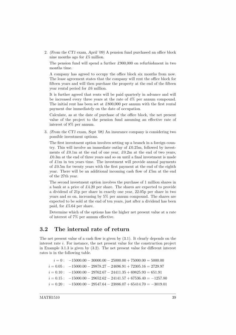
2. (From the CT1 exam, April ’09) A pension fund purchased an office blocknine months ago for £5 million.

The pension fund will spend a further £900,000 on refurbishment in twomonths time.

A company has agreed to occupy the office block six months from now.The lease agreement states that the company will rent the office block forfifteen years and will then purchase the property at the end of the fifteenyear rental period for £6 million.

It is further agreed that rents will be paid quarterly in advance and willbe increased every three years at the rate of 4% per annum compound.The initial rent has been set at £800,000 per annum with the first rentalpayment due immediately on the date of occupation.

Calculate, as at the date of purchase of the office block, the net presentvalue of the project to the pension fund assuming an effective rate ofinterest of 8% per annum.

3. (From the CT1 exam, Sept ’08) An insurance company is considering twopossible investment options.

The first investment option involves setting up a branch in a foreign coun-try. This will involve an immediate outlay of £0.25m, followed by invest-ments of £0.1m at the end of one year, £0.2m at the end of two years,£0.3m at the end of three years and so on until a final investment is madeof £1m in ten years time. The investment will provide annual paymentsof £0.5m for twenty years with the first payment at the end of the eighthyear. There will be an additional incoming cash flow of £5m at the endof the 27th year.

The second investment option involves the purchase of 1 million shares ina bank at a price of £4.20 per share. The shares are expected to providea dividend of 21p per share in exactly one year, 22.05p per share in twoyears and so on, increasing by 5% per annum compound. The shares areexpected to be sold at the end of ten years, just after a dividend has beenpaid, for £5.64 per share.

Determine which of the options has the higher net present value at a rateof interest of 7% per annum effective.

3.2 The internal rate of return

The net present value of a cash flow is given by (3.1). It clearly depends on theinterest rate i. For instance, the net present value for the construction projectin Example 3.1.3 is given by (3.2). The net present value for different interestrates is in the following table.

i = 0 : −15000.00− 30000.00− 25000.00 + 75000.00 = 5000.00i = 0.05 : −15000.00− 29878.27− 24696.91 + 72305.16 = 2729.97i = 0.10 : −15000.00− 29762.67− 24411.35 + 69825.93 = 651.91i = 0.15 : −15000.00− 29652.62− 24141.57 + 67536.40 = −1257.80i = 0.20 : −15000.00− 29547.64− 23886.07 + 65414.70 = −3019.01

MATH1510 39

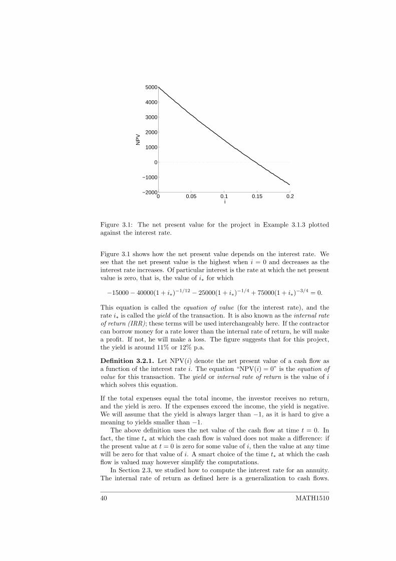
0 0.05 0.1 0.15 0.2−2000

−1000

0

1000

2000

3000

4000

5000

i

NP

V

Figure 3.1: The net present value for the project in Example 3.1.3 plottedagainst the interest rate.

Figure 3.1 shows how the net present value depends on the interest rate. Wesee that the net present value is the highest when i = 0 and decreases as theinterest rate increases. Of particular interest is the rate at which the net presentvalue is zero, that is, the value of i∗ for which

−15000− 40000(1 + i∗)−1/12 − 25000(1 + i∗)−1/4 + 75000(1 + i∗)−3/4 = 0.

This equation is called the equation of value (for the interest rate), and therate i∗ is called the yield of the transaction. It is also known as the internal rateof return (IRR); these terms will be used interchangeably here. If the contractorcan borrow money for a rate lower than the internal rate of return, he will makea profit. If not, he will make a loss. The figure suggests that for this project,the yield is around 11% or 12% p.a.

Definition 3.2.1. Let NPV(i) denote the net present value of a cash flow asa function of the interest rate i. The equation “NPV(i) = 0” is the equation ofvalue for this transaction. The yield or internal rate of return is the value of iwhich solves this equation.

If the total expenses equal the total income, the investor receives no return,and the yield is zero. If the expenses exceed the income, the yield is negative.We will assume that the yield is always larger than −1, as it is hard to give ameaning to yields smaller than −1.

The above definition uses the net value of the cash flow at time t = 0. Infact, the time t∗ at which the cash flow is valued does not make a difference: ifthe present value at t = 0 is zero for some value of i, then the value at any timewill be zero for that value of i. A smart choice of the time t∗ at which the cashflow is valued may however simplify the computations.

In Section 2.3, we studied how to compute the interest rate for an annuity.The internal rate of return as defined here is a generalization to cash flows.

40 MATH1510

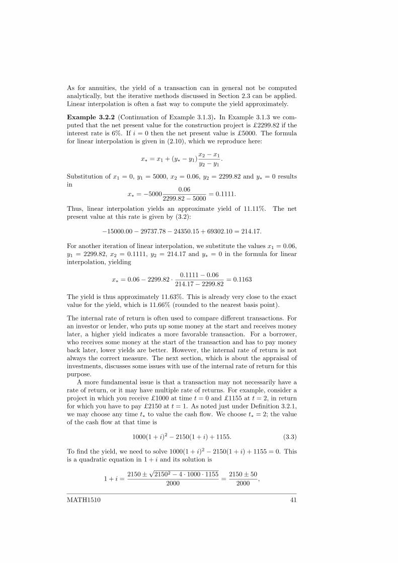
As for annuities, the yield of a transaction can in general not be computedanalytically, but the iterative methods discussed in Section 2.3 can be applied.Linear interpolation is often a fast way to compute the yield approximately.

Example 3.2.2 (Continuation of Example 3.1.3). In Example 3.1.3 we com-puted that the net present value for the construction project is £2299.82 if theinterest rate is 6%. If i = 0 then the net present value is £5000. The formulafor linear interpolation is given in (2.10), which we reproduce here:

x∗ = x1 + (y∗ − y1)x2 − x1

y2 − y1.

Substitution of x1 = 0, y1 = 5000, x2 = 0.06, y2 = 2299.82 and y∗ = 0 resultsin

x∗ = −50000.06

2299.82− 5000= 0.1111.

Thus, linear interpolation yields an approximate yield of 11.11%. The netpresent value at this rate is given by (3.2):

−15000.00− 29737.78− 24350.15 + 69302.10 = 214.17.

For another iteration of linear interpolation, we substitute the values x1 = 0.06,y1 = 2299.82, x2 = 0.1111, y2 = 214.17 and y∗ = 0 in the formula for linearinterpolation, yielding

x∗ = 0.06− 2299.82 · 0.1111− 0.06214.17− 2299.82

= 0.1163

The yield is thus approximately 11.63%. This is already very close to the exactvalue for the yield, which is 11.66% (rounded to the nearest basis point).

The internal rate of return is often used to compare different transactions. Foran investor or lender, who puts up some money at the start and receives moneylater, a higher yield indicates a more favorable transaction. For a borrower,who receives some money at the start of the transaction and has to pay moneyback later, lower yields are better. However, the internal rate of return is notalways the correct measure. The next section, which is about the appraisal ofinvestments, discusses some issues with use of the internal rate of return for thispurpose.

A more fundamental issue is that a transaction may not necessarily have arate of return, or it may have multiple rate of returns. For example, consider aproject in which you receive £1000 at time t = 0 and £1155 at t = 2, in returnfor which you have to pay £2150 at t = 1. As noted just under Definition 3.2.1,we may choose any time t∗ to value the cash flow. We choose t∗ = 2; the valueof the cash flow at that time is

1000(1 + i)2 − 2150(1 + i) + 1155. (3.3)

To find the yield, we need to solve 1000(1 + i)2 − 2150(1 + i) + 1155 = 0. Thisis a quadratic equation in 1 + i and its solution is

1 + i =2150±

√21502 − 4 · 1000 · 1155

2000=

2150± 502000

,

MATH1510 41

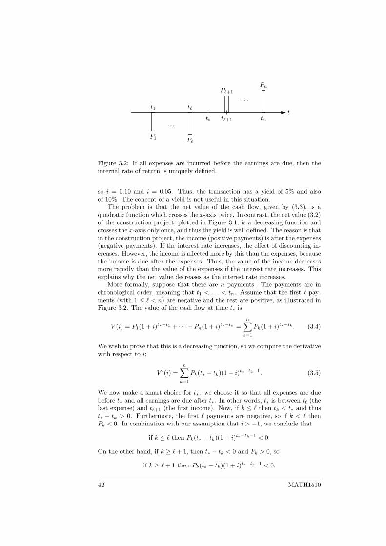
tt1 t`

t∗ t`+1 tn

P`+1

P1 P`

Pn

· · ·

· · ·

Figure 3.2: If all expenses are incurred before the earnings are due, then theinternal rate of return is uniquely defined.

so i = 0.10 and i = 0.05. Thus, the transaction has a yield of 5% and alsoof 10%. The concept of a yield is not useful in this situation.

The problem is that the net value of the cash flow, given by (3.3), is aquadratic function which crosses the x-axis twice. In contrast, the net value (3.2)of the construction project, plotted in Figure 3.1, is a decreasing function andcrosses the x-axis only once, and thus the yield is well defined. The reason is thatin the construction project, the income (positive payments) is after the expenses(negative payments). If the interest rate increases, the effect of discounting in-creases. However, the income is affected more by this than the expenses, becausethe income is due after the expenses. Thus, the value of the income decreasesmore rapidly than the value of the expenses if the interest rate increases. Thisexplains why the net value decreases as the interest rate increases.

More formally, suppose that there are n payments. The payments are inchronological order, meaning that t1 < . . . < tn. Assume that the first ` pay-ments (with 1 ≤ ` < n) are negative and the rest are positive, as illustrated inFigure 3.2. The value of the cash flow at time t∗ is

V (i) = P1(1 + i)t∗−t1 + · · ·+ Pn(1 + i)t∗−tn =n∑k=1

Pk(1 + i)t∗−tk . (3.4)

We wish to prove that this is a decreasing function, so we compute the derivativewith respect to i:

V ′(i) =n∑k=1

Pk(t∗ − tk)(1 + i)t∗−tk−1. (3.5)

We now make a smart choice for t∗: we choose it so that all expenses are duebefore t∗ and all earnings are due after t∗. In other words, t∗ is between t` (thelast expense) and t`+1 (the first income). Now, if k ≤ ` then tk < t∗ and thust∗ − tk > 0. Furthermore, the first ` payments are negative, so if k < ` thenPk < 0. In combination with our assumption that i > −1, we conclude that

if k ≤ ` then Pk(t∗ − tk)(1 + i)t∗−tk−1 < 0.

On the other hand, if k ≥ `+ 1, then t∗ − tk < 0 and Pk > 0, so

if k ≥ `+ 1 then Pk(t∗ − tk)(1 + i)t∗−tk−1 < 0.

42 MATH1510

This mean that all terms in the sum in (3.5) are negative, Thus, V ′(i) < 0; thenet value is a decreasing function with respect to the interest rate. This meansthat the graph of V (i) can cross the x-axis at most once, so the internal rate ofreturn is unique.

This does not show that the graph of V (i) does in fact cross the x-axis. Forthat, we compute the value of the cash flow in the limits i ↓ −1 and i → +∞.In the limit i ↓ −1 (that is, i approaches −1 from above), 1 + i is small butpositive. We have

limi↓−1

(1 + i)a =

{+∞, if a < 0;0, if a > 0.

The kth term in the sum (3.4) for V (i) is Pk(1 + i)t∗−tk . First consider the casek ≤ `. The exponent t∗− tk is positive if k ≤ `, so Pk(1 + i)t∗−tk → 0 as i ↓ −1.In the case k ≥ ` + 1, the exponent t∗ − tk is negative, and Pk is positive, soPk(1 + i)t∗−tk → +∞ as i ↓ −1. Adding all terms, we find that V (i)→ +∞ inthe limit i ↓ −1.

Next, consider the limit i→∞. Now we have

limi→∞

(1 + i)a =

{0, if a < 0;+∞, if a > 0.

Thus, Pk(1 + i)t∗−tk → −∞ if k ≤ ` and Pk(1 + i)t∗−tk → 0 if k ≥ ` + 1. Wefind that

limi↓−1

V (i) = +∞ and limi→∞

V (i) = −∞.

Since V (i) goes from +∞ to −∞, there must be an i ∈ (−1,∞) for whichV (i) = 0. Thus, the internal rate of return exists and is unique.

The above discussion shows that a cash flow where all expenses are incurredbefore the earnings are due has a well-defined yield. The same is true in thereverse situation, where all earnings are due before the expenses are incurred,as happens for instance when borrowing money. The proof is very similar.

There is another situation in which the yield is well-defined, namely, if allcumulative payments before a certain time t∗ are negative and all cumulativepayments afterwards are positive (or the other way around, with all cumulativepayments before t∗ positive and all after t∗ negative). The kth cumulativepayment Ck is the sum of the first k payments:

Ck =k∑j=1

Pj . (3.6)

Thus, Ck is the total amount the investor has received at the time of the kthpayment. If there is one and only one time at which the cumulative cash flowchanges sign, then there is only one positive value of i for which the net valueof the cash flow is zero. We will not prove this result in these lecture notes.

MATH1510 43

Example 3.2.3. A cash flow with payments −5, 3, −1, 7, −1 and 3 after 0,2, 3, 7, 8 and 10 years, respectively, has cumulative payments as shown in thetable below:

k tk Pk Ck1 0 −5 −52 2 3 −23 3 −1 −34 7 7 45 8 −1 36 10 3 6

Even though the negative and positive payments are interleaved, all negative Ckare before the positive Ck. After seven years, at the time of the fourth payment,the cumulative cash flow changes from negative to positive (as explained in thenext section, this time is called the payback period). Thus the yield of this cashflow is well defined. A computation as in Example 3.2.2 shows that the yield isapproximately 13.55% p.a.

The two situations discussed above (payments change sign only once, and cu-mulative payments change sign only once) cover many cash flows occurring inpractice. The internal rate of return of a investment project is usually welldefined.

3.3 Investment project appraisal

Section 3.1 defined the net present value of a cash flow, while Section 3.2 dis-cussed the internal rate of return. Both quantities are often used to evaluateand compare investments and other projects. Project with higher net presentvalues and yields are more profitable to invest in.

If, as in many investments, there is a period of outlays followed by a periodof profits, then the net present value is a decreasing function of the interest rate.The net present value is positive, and thus the project profitable, if the investorcan borrow and lend money at a rate smaller than the internal rate of return.Thus, a project with a higher yield has more chance to be profitable.

This does not mean, however, that a project with a higher yield will alwaysbe more profitable than a project with a lower yield. It is the project with thehigher net value for a given interest rate that is the most profitable.

Example 3.3.1 (McCutcheon & Scott, p. 92). An investor is contemplating twoinvestment projects. Project A requires an initial payment of £10000, in returnfor which the investor will receive £250 at the end of every quarter for 15 years.Project B requires an initial payment of £11000. In return, the investor willbe paid £605 at the end of every year for 18 years and the initial payment of£11000 will be repaid at the end.

Both projects have one outlay at the start, and payments to the investorafterwards, so they both have a well-defined internal rate of return. The netpresent value for Project A is given by

NPVA(i) = −10000 + 1000a(4)

15.

44 MATH1510

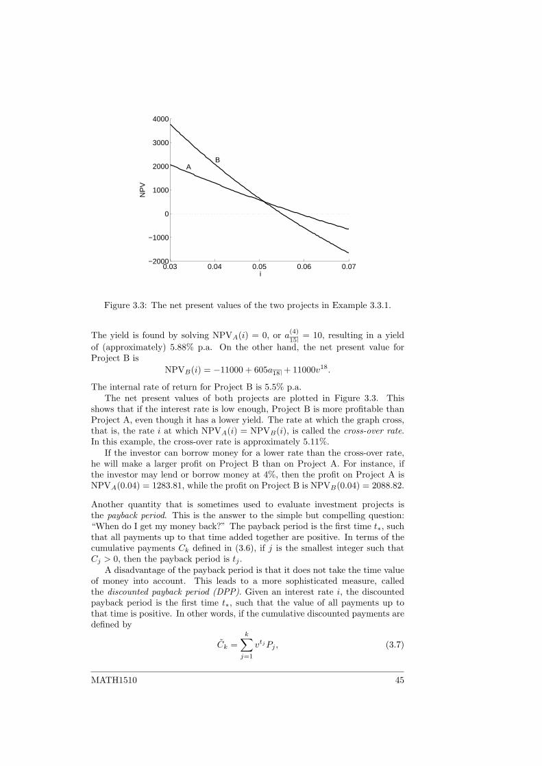
0.03 0.04 0.05 0.06 0.07−2000

−1000

0

1000

2000

3000

4000

BA

i

NP

V

Figure 3.3: The net present values of the two projects in Example 3.3.1.

The yield is found by solving NPVA(i) = 0, or a(4)

15= 10, resulting in a yield

of (approximately) 5.88% p.a. On the other hand, the net present value forProject B is

NPVB(i) = −11000 + 605a18 + 11000v18.

The internal rate of return for Project B is 5.5% p.a.The net present values of both projects are plotted in Figure 3.3. This

shows that if the interest rate is low enough, Project B is more profitable thanProject A, even though it has a lower yield. The rate at which the graph cross,that is, the rate i at which NPVA(i) = NPVB(i), is called the cross-over rate.In this example, the cross-over rate is approximately 5.11%.

If the investor can borrow money for a lower rate than the cross-over rate,he will make a larger profit on Project B than on Project A. For instance, ifthe investor may lend or borrow money at 4%, then the profit on Project A isNPVA(0.04) = 1283.81, while the profit on Project B is NPVB(0.04) = 2088.82.

Another quantity that is sometimes used to evaluate investment projects isthe payback period. This is the answer to the simple but compelling question:“When do I get my money back?” The payback period is the first time t∗, suchthat all payments up to that time added together are positive. In terms of thecumulative payments Ck defined in (3.6), if j is the smallest integer such thatCj > 0, then the payback period is tj .

A disadvantage of the payback period is that it does not take the time valueof money into account. This leads to a more sophisticated measure, calledthe discounted payback period (DPP). Given an interest rate i, the discountedpayback period is the first time t∗, such that the value of all payments up tothat time is positive. In other words, if the cumulative discounted payments aredefined by

Ck =k∑j=1

vtjPj , (3.7)

MATH1510 45

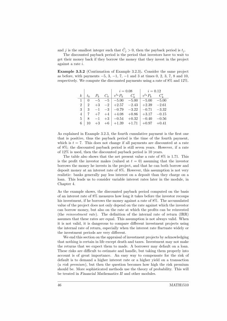
and j is the smallest integer such that Cj > 0, then the payback period is tj .The discounted payback period is the period that investors have to wait to

get their money back if they borrow the money that they invest in the projectagainst a rate i.

Example 3.3.2 (Continuation of Example 3.2.3). Consider the same projectas before, with payments −5, 3, −1, 7, −1 and 3 at times 0, 2, 3, 7, 8 and 10,respectively. We compute the discounted payments using a rate of 8% and 12%.

i = 0.08 i = 0.12k tk Pk Ck vtkPk C ′k vtkPk C ′k1 0 −5 −5 −5.00 −5.00 −5.00 −5.002 2 +3 −2 +2.57 −2.43 +2.39 −2.613 3 −1 −3 −0.79 −3.22 −0.71 −3.324 7 +7 +4 +4.08 +0.86 +3.17 −0.155 8 −1 +3 −0.54 +0.32 −0.40 −0.566 10 +3 +6 +1.39 +1.71 +0.97 +0.41

As explained in Example 3.2.3, the fourth cumulative payment is the first onethat is positive, thus the payback period is the time of the fourth payment,which is t = 7. This does not change if all payments are discounted at a rateof 8%; the discounted payback period is still seven years. However, if a rateof 12% is used, then the discounted payback period is 10 years.

The table also shows that the net present value a rate of 8% is 1.71. Thisis the profit the investor makes (valued at t = 0) assuming that the investorborrows the money he invests in the project, and that he can both borrow anddeposit money at an interest rate of 8%. However, this assumption is not veryrealistic: banks generally pay less interest on a deposit than they charge on aloan. This leads us to consider variable interest rates later in the module, inChapter 4.

As the example shows, the discounted payback period computed on the basisof an interest rate of 8% measures how long it takes before the investor recoupshis investment, if he borrows the money against a rate of 8%. The accumulatedvalue of the project does not only depend on the rate against which the investorcan borrow money, but also on the rate at which the profits can be reinvested(the reinvestment rate). The definition of the internal rate of return (IRR)assumes that these rates are equal. This assumption is not always valid. Whenit is not valid, it is dangerous to compare different investment projects usingthe internal rate of return, especially when the interest rate fluctuate widely orthe investment periods are very different.

We end this section on the appraisal of investment projects by acknowledgingthat nothing is certain in life except death and taxes. Investment may not makethe returns that we expect them to made. A borrower may default on a loan.These risks are difficult to estimate and handle, but taking them properly intoaccount is of great importance. An easy way to compensate for the risk ofdefault is to demand a higher interest rate or a higher yield on a transaction(a risk premium), but then the question becomes how high the risk premiumshould be. More sophisticated methods use the theory of probability. This willbe treated in Financial Mathematics II and other modules.

46 MATH1510

3.4 Investment funds

An investment fund is a collective scheme which pools and invests money frommultiple parties. The pool of money administered by the fund changes over time.This complicates the assessment of the performance of an investment fund. Thevalue of the fund changes not only due to the performance of its investments,but also due to additional investments or withdrawals by its members.

The following example shows that the internal rate of return can be used toassess the performance of an investment fund.

Example 3.4.1. Consider an investment fund that starts out with £100,000.After one year, this has increased to £105,000. The investors deposit an addi-tional £50,000 to the funds, so the total sum administered is now £155,000. Thesecond years turns out to be very profitable: the value of the funds increasesto £195,000. At this time, the investors withdraw £60,000, leaving £135,000in the funds. Unfortunately, the investments go sour in the third year, and thevalue of the funds decreases to £125,000. What is the yield achieved by theinvestment fund over these three years?

Answer. If the fund would be wound up, the fund would have to pay £125,000back to the investors. Thus, the cash flow is +100 (measured in thousandsof pounds) at t = 0 (measured in years), +50 at t = 1, −60 at t = 2 and−125 at t = 3. The equation of value at t = 0 is

100 + 50(1 + i)−1 − 60(1 + i)−2 − 125(1 + i)−3 = 0. (3.8)

The solution of this equation is i = 0.0937, so the yield rate is 9.37%.

The fund manager in the example achieved a return of 5100 = 5% in the first

year, 40155 = 25.81% in the second year, and − 10

135 = −7.41% in the third year.If you invest money against these rates, the yield over three years is((

1 +5

100

)(1 +

40155

)(1− 10

135

))1/3

− 1 = (1.223118)1/3 − 1 = 0.0694,

or 6.94%. The yield rate of 9.37% that was computed in the example is consid-erably higher because that computation gives more weight to periods in whichmore money is invested in the funds. In the example, the second year has themost money in the funds, so that year has more influence on the yield rate thanthe first and last year. Coincidentally, the funds performed considerably betterin the second year than in the first and last year. This explains why the yieldrate is so high.

Because the internal rate of return gives more weight to periods in whichmore money is invested in the funds, it is often called the money-weighted rateof return in this context. Yet another name is the dollar-weighted rate of return,though this is obviously not appropriate for British funds. In contrast, the rateof 6.94% is called the time-weighted rate of return. The time-weighted rateof return is a fairer measure of the performance of a fund manager, becauseit eliminates the effect of investors depositing or withdrawing money from thefunds. However, the money-weighted computation is a valid measure of theactual investment results achieved.

The formal definitions of the money-weighted rate of return and the time-weighted rate of return are as follows.

MATH1510 47

Definition 3.4.2. Let Vk with k = 0, 1, . . . , n denote the value of an investmentfund at time tk, where the times are ordered such that t0 < t1 < . . . < tn. Letck with k = 1, 2, . . . , n1 denote the new cash deposited into the fund at time tk(if ck < 0 then cash is withdrawn). The value Vk is measured just before thenew cash is deposited or withdrawn. The money-weighted rate of return is therate i which satisfies

V0(1 + i)tn−t0 + c1(1 + i)tn−t1

+ c2(1 + i)tn−t2 + · · ·+ cn−1(1 + i)tn−tn−1 = Vn. (3.9)

The time-weighted rate of return is the rate i which satisfies

(1 + i)tn−t0 =V1

V0· V2

V1 + c1· V3

V2 + c2· · · Vn

Vn−1 + cn−1. (3.10)

Example 3.4.3 (Continuation of Example 3.4.1). In the situation of Exam-ple 3.4.1, the value of the fund is V0 = 100000, V1 = 105000, V2 = 155000 andV3 = 125000 at times t0 = 0, t1 = 1, t2 = 2 and t3 = 3, respectively. The flowof new money is given by c1 = 50000 and c2 = −60000. Thus, equation (3.9)for the money-weighted rate of return gives

100000(1 + i)3 + 50000(1 + i)2 − 60000(1 + i) = 125000.

This is equivalent to equation (3.10) which we found before; the money-weightedrate of return is 9.37%.

Equation (3.10) for the time-weighted rate of return gives

(1 + i)3 =105000100000

· 195000105000 + 50000

· 125000195000− 60000

.

The solution of this equation is i = 0.0694, so the time-weighted rate of returnis 6.94%, as we found before.

The linked internal rate of return is another measure that is sometimes used.It is a variant of the time-weighted rate of return which approximates the flowof new money into and out of the funds. We will not be considering the linkedinternal rate of return in this module.

Exercises

1. (From the CT1 exam, April ’09) A fund had a value of £150,000 on 1July 2006. A net cash flow of £30,000 was received on 1 July 2007 and afurther net cash flow of £40,000 was received on 1 July 2008. The fundhad a value of £175,000 on 30 June 2007 and a value of £225,000 on 30June 2008. The value of the fund on 1 January 2009 was £280,000.

(a) Calculate the time-weighted rate of return per annum earned on thefund between 1 July 2006 and 1 January 2009.

(b) Calculate the money-weighted rate of return per annum earned onthe fund between 1 July 2006 and 1 January 2009.

(c) Explain why the time-weighted rate of return is more appropriatethan the money-weighted rate of return when comparing the perfor-mance of two investment managers over the same period of time.

48 MATH1510

2. (From the CT1 exam, Sept ’08) An investor had savings totalling £41,000in an account on 1 January 2006. He invested a further £12,000 in thisaccount on 1 August 2006. The total value of the account was £45,000 on31 July 2006 and was £72,000 on 31 December 2007.

Assuming that the investor made no further deposits or withdrawals inrelation to this account, calculate the annual effective time-weighted rateof return for the period 1 January 2006 to 31 December 2007.

3.5 Bonds

A bond is a certificate of indebtedness issued by a borrower. It promises to paya certain amount of money at a specified date (or several amounts at severaldates). If a company or government agency wants to borrow money, it can goto a bank or it can issue bonds and sell these to investors. Bonds are usuallyissued for a round value such as £100 in the U.K. and $1000 in the U.S.; this iscalled the face value of the bond.

Most bonds specify when the loan is paid back. This is called the maturitydate, and the period between the issue of the bond and its maturity is the termof the bond. The amount paid to the investor at the maturity date is called theredemption value of the bond. The redemption value usually equals the facevalue; in this case the bond is said to be redeemed at par. We will assume inthis module that all bonds are redeemed at par.

Many bonds also pay interest on the loan in addition to repaying it at matu-rity. These interest payments are called coupons. The coupons are computed bymultiplying an interest rate specified on the bond (the coupon rate) by the facevalue. Thus, a bond with a coupon rate of 8% and a face value of £100 wouldpay coupons of £8 if the coupons are paid annually. Typically, coupons arepayable semi-annually and the nominal rate is quoted, so a bond with couponsof 8% payable semi-annually pays coupons of £4 every half year.

Governments usually have to raise large sums of money and they do this byissuing bonds. Bonds issued by the U.K. government are known as gilts. Bondsissued by the U.S. governments are called Treasury notes if the term is relativelylong, and Treasury bills (or T-bills) if the term is relatively short.

A fundamental computation is to compute the price an investor has to payfor a bond to achieve a certain yield. The basic rule is that the price of thebond must be equal to the present value of the coupons plus the present valueof the redemption value, where the present values are computed using the givenyield rate.

Example 3.5.1. Find the price of a five-year bond with a face value of £100and coupons at 8% p.a. payable semi-annually. The bond is redeemable at parand bought to yield 5%.

Answer. The investor will receive half-yearly payments of £4 for five years.We use time units of a year. The present value of these payments is 8a(2)

5

(remember that a(2)n is the present value of semi-annual payments of a half ).

Additionally, the investor will receive £100 at maturity; the present value ofthis payment is 100v5. Here, the yield rate is given as i = 0.05, so v = 0.952381and i(2) = 0.0493901. We compute the present value of both the coupons and

MATH1510 49

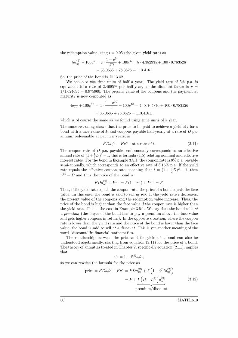
the redemption value using i = 0.05 (the given yield rate) as

8a(2)

5+ 100v5 = 8 · 1− v5

i(2)+ 100v5 = 8 · 4.382935 + 100 · 0.783526

= 35.0635 + 78.3526 = 113.4161.

So, the price of the bond is £113.42.We can also use time units of half a year. The yield rate of 5% p.a. is

equivalent to a rate of 2.4695% per half-year, so the discount factor is v =1/1.024695 = 0.975900. The present value of the coupons and the payment atmaturity is now computed as

4a10 + 100v10 = 4 · 1− v10

i+ 100v10 = 4 · 8.765870 + 100 · 0.783526

= 35.0635 + 78.3526 = 113.4161,

which is of course the same as we found using time units of a year.

The same reasoning shows that the price to be paid to achieve a yield of i for abond with a face value of F and coupons payable half-yearly at a rate of D perannum, redeemable at par in n years, is

FDa(2)n + Fvn at a rate of i. (3.11)

The coupon rate of D p.a. payable semi-annually corresponds to an effectiveannual rate of (1 + 1

2D)2−1; this is formula (1.5) relating nominal and effectiveinterest rates. For the bond in Example 3.5.1, the coupon rate is 8% p.a. payablesemi-annually, which corresponds to an effective rate of 8.16% p.a. If the yieldrate equals the effective coupon rate, meaning that i = (1 + 1

2D)2 − 1, theni(2) = D and thus the price of the bond is

FDa(2)n + Fvn = F (1− vn) + Fvn = F.

Thus, if the yield rate equals the coupon rate, the price of a bond equals the facevalue. In this case, the bond is said to sell at par. If the yield rate i decreases,the present value of the coupons and the redemption value increase. Thus, theprice of the bond is higher than the face value if the coupon rate is higher thanthe yield rate. This is the case in Example 3.5.1. We say that the bond sells ata premium (the buyer of the bond has to pay a premium above the face valueand gets higher coupons in return). In the opposite situation, where the couponrate is lower than the yield rate and the price of the bond is lower than the facevalue, the bond is said to sell at a discount. This is yet another meaning of theword “discount” in financial mathematics.

The relationship between the price and the yield of a bond can also beunderstood algebraically, starting from equation (3.11) for the price of a bond.The theory of annuities treated in Chapter 2, specifically equation (2.11), impliesthat

vn = 1− i(2)a(2)n ,

so we can rewrite the formula for the price as

price = FDa(2)n + Fvn = FDa

(2)n + F

(1− i(2)a(2)

n

)= F + F

(D − i(2)

)a(2)n︸ ︷︷ ︸

premium/discount

(3.12)

50 MATH1510

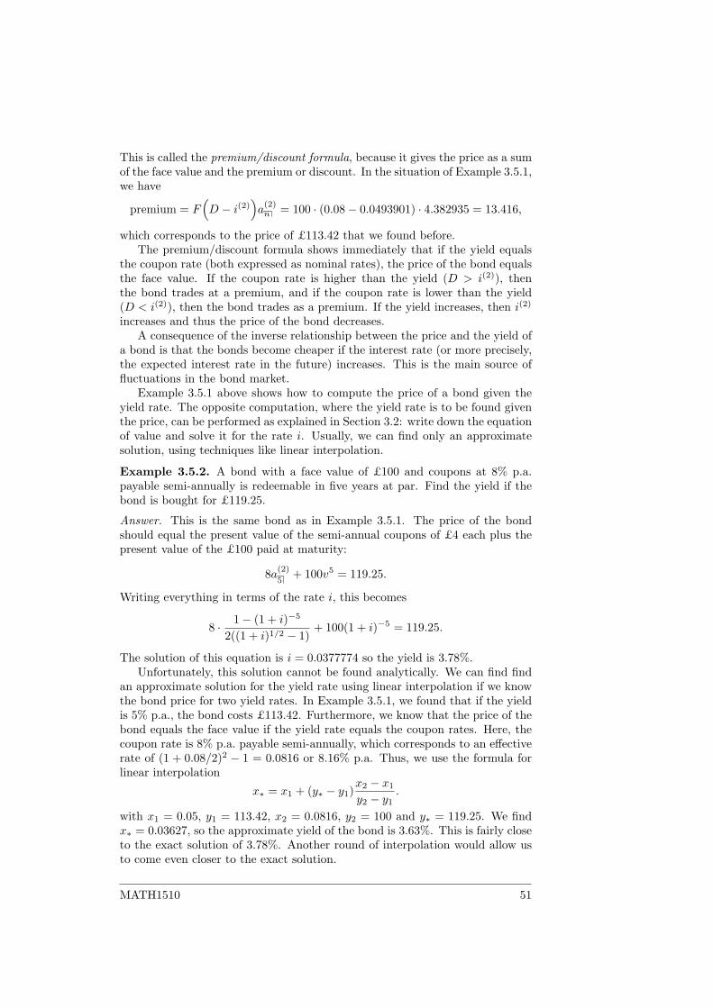
This is called the premium/discount formula, because it gives the price as a sumof the face value and the premium or discount. In the situation of Example 3.5.1,we have

premium = F(D − i(2)

)a(2)n = 100 · (0.08− 0.0493901) · 4.382935 = 13.416,

which corresponds to the price of £113.42 that we found before.The premium/discount formula shows immediately that if the yield equals

the coupon rate (both expressed as nominal rates), the price of the bond equalsthe face value. If the coupon rate is higher than the yield (D > i(2)), thenthe bond trades at a premium, and if the coupon rate is lower than the yield(D < i(2)), then the bond trades as a premium. If the yield increases, then i(2)

increases and thus the price of the bond decreases.A consequence of the inverse relationship between the price and the yield of

a bond is that the bonds become cheaper if the interest rate (or more precisely,the expected interest rate in the future) increases. This is the main source offluctuations in the bond market.

Example 3.5.1 above shows how to compute the price of a bond given theyield rate. The opposite computation, where the yield rate is to be found giventhe price, can be performed as explained in Section 3.2: write down the equationof value and solve it for the rate i. Usually, we can find only an approximatesolution, using techniques like linear interpolation.

Example 3.5.2. A bond with a face value of £100 and coupons at 8% p.a.payable semi-annually is redeemable in five years at par. Find the yield if thebond is bought for £119.25.

Answer. This is the same bond as in Example 3.5.1. The price of the bondshould equal the present value of the semi-annual coupons of £4 each plus thepresent value of the £100 paid at maturity:

8a(2)

5+ 100v5 = 119.25.

Writing everything in terms of the rate i, this becomes

8 · 1− (1 + i)−5

2((1 + i)1/2 − 1)+ 100(1 + i)−5 = 119.25.

The solution of this equation is i = 0.0377774 so the yield is 3.78%.Unfortunately, this solution cannot be found analytically. We can find find

an approximate solution for the yield rate using linear interpolation if we knowthe bond price for two yield rates. In Example 3.5.1, we found that if the yieldis 5% p.a., the bond costs £113.42. Furthermore, we know that the price of thebond equals the face value if the yield rate equals the coupon rates. Here, thecoupon rate is 8% p.a. payable semi-annually, which corresponds to an effectiverate of (1 + 0.08/2)2 − 1 = 0.0816 or 8.16% p.a. Thus, we use the formula forlinear interpolation

x∗ = x1 + (y∗ − y1)x2 − x1

y2 − y1.

with x1 = 0.05, y1 = 113.42, x2 = 0.0816, y2 = 100 and y∗ = 119.25. We findx∗ = 0.03627, so the approximate yield of the bond is 3.63%. This is fairly closeto the exact solution of 3.78%. Another round of interpolation would allow usto come even closer to the exact solution.

MATH1510 51

70 80 90 100 110 120 130 1400

2

4

6

8

10

12

14

16

yiel

d (%

)

price

Figure 3.4: The relation between the price and the yield of a five-year bond witha face value of £100 and coupons at 8% p.a. payable semi-annually (as treatedin the examples in this section). If the price increases, the yield decreases, andvice versa.

As illustrated in the example, the yield of a bond that is trading at a premium(that is, the price is higher than the face value) is lower than the coupon rate.The relation between yield and price is shown in Figure 3.4.

A source of confusion is the difference between effective and nominal rates.The coupon rate is always quoted as a nominal rate, convertible with the samefrequency as the coupon payments. The yield rate of 3.78% computed in theabove example is an effective rate. The corresponding nominal rate is

2((1 + 0.0378)1/2 − 1

)= 0.0374 or 3.74%.

When comparing two rates, you should make sure they both are both effectiverates or that they both are nominal rates convertible with the same frequency.Thus, in the premium/discount formula, equation (3.12), the coupon rate andyield are both nominal rates. Bond yields in the financial press are usuallyquoted using nominal rates. This is appropriate when comparing different bondsbecause (almost) all bonds pay coupons with the same frequency. However,when comparing bond yields with yields on other investments, the bond yieldhas to be converted to an effective annual rate.

Another source of confusion is that people sometimes consider another yieldrate called the interest yield. This is the yield computed on the basis of only theinterest payments, while ignoring the redemption value. The interest yield of thebond in Example 3.5.2, which has a coupon rate of 8% and trades at £119.25,is 8/119.25 = 0.0671 or 6.71%. This rate is the nominal rate p.a. convertiblesemi-annually; the effective rate is 6.82%. The interest yield is also known asthe flat yield. The yield that we considered in the rest of this section, whichdoes take the redemption value into account, is sometimes called the redemptionyield or the yield to maturity if it is necessary to distinguish it from the interest

52 MATH1510

0 5 10 15 20100

110

120

130

140

pric

e

term to redemption0 5 10 15 20

0

2

4

6

8

yiel

d (%

)

term to redemption

Figure 3.5: The relation between the redemption term and the price and yieldof a bond. Consider a bound with a face value of £100 and a coupon rate of 8%payable semi-annually, whose redemption term varies. The left plot shows theprice of the bond if it is bought to yield 5%, as in Example 3.5.1. The right plotshows the yield of the bond if it is bought for £119.25, as in Example 3.5.2.

yield.

If a bond is trading at a premium then the investor will receive less moneyat maturity than he paid for the bond, so he will suffer a loss at maturity.Thus, the redemption yield is lower than the interest yield for bonds tradingat a premium. On the other hand, the coupon rate is higher than the interestyield for bonds trading at a premium: the interest yield is the coupon paymentsdivided by the price of the bond, while the coupon rate is the coupon paymentsdivided by the face value, and the price is higher than the face value becausethe bond trades at a premium. This is the case in Example 3.5.2, where thebond has a redemption yield of 3.74%, an interest yield of 6.71%, and a couponrate of 8% (all quoted as nominal rates). Conversely, the redemption yield ishigher than the interest yield which is higher than the coupon rate when thebond is trading at a discount.

The difference between the redemption yield and the interest yield dependson the term to redemption. If it takes very long before the bond matures,then the present value of the profit or loss for the investor at maturity is small,because it is discounted for a very long time. Thus, the difference betweenthe redemption yield and the interest yield decreases as the redemption termincreases. In the limit n→∞, the bond never matures (so the coupons form aperpetuity), and the redemption and interest yields are the same.

If a bond is trading at a premium, then the redemption yield is lower thanthe interest yield. Since the redemption yield approaches the interest yieldas the redemption term increases, and the interest yield stays constant, theredemption yield must increase. This is shown in the right plot of Figure 3.5,which illustrate the influence of the redemption term on the yield of the bondin Example 3.5.2, which is trading at a premium. In the opposite situation, thebond is trading at a discount, the redemption yield is higher than the interestyield, and the redemption yield decreases as the redemption term increases.

The effect of the term to redemption on the price can be seen from for-

MATH1510 53

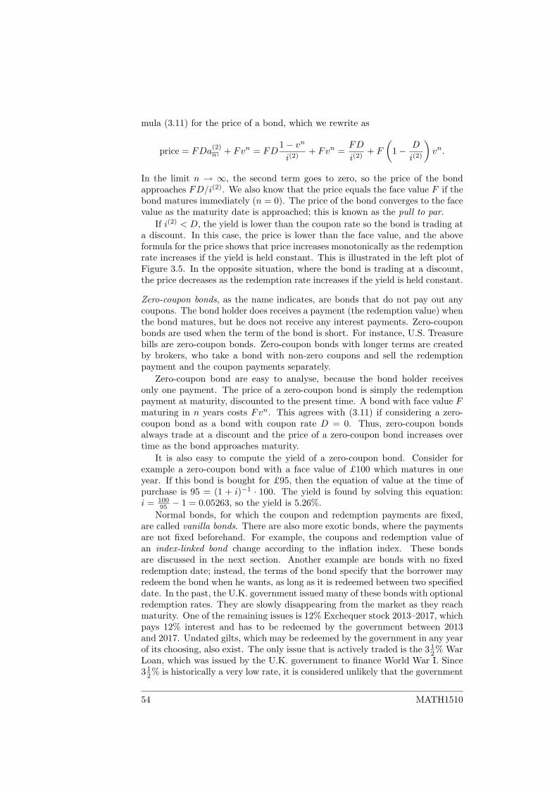
mula (3.11) for the price of a bond, which we rewrite as

price = FDa(2)n + Fvn = FD

1− vn

i(2)+ Fvn =

FD

i(2)+ F

(1− D

i(2)

)vn.

In the limit n → ∞, the second term goes to zero, so the price of the bondapproaches FD/i(2). We also know that the price equals the face value F if thebond matures immediately (n = 0). The price of the bond converges to the facevalue as the maturity date is approached; this is known as the pull to par.

If i(2) < D, the yield is lower than the coupon rate so the bond is trading ata discount. In this case, the price is lower than the face value, and the aboveformula for the price shows that price increases monotonically as the redemptionrate increases if the yield is held constant. This is illustrated in the left plot ofFigure 3.5. In the opposite situation, where the bond is trading at a discount,the price decreases as the redemption rate increases if the yield is held constant.

Zero-coupon bonds, as the name indicates, are bonds that do not pay out anycoupons. The bond holder does receives a payment (the redemption value) whenthe bond matures, but he does not receive any interest payments. Zero-couponbonds are used when the term of the bond is short. For instance, U.S. Treasurebills are zero-coupon bonds. Zero-coupon bonds with longer terms are createdby brokers, who take a bond with non-zero coupons and sell the redemptionpayment and the coupon payments separately.

Zero-coupon bond are easy to analyse, because the bond holder receivesonly one payment. The price of a zero-coupon bond is simply the redemptionpayment at maturity, discounted to the present time. A bond with face value Fmaturing in n years costs Fvn. This agrees with (3.11) if considering a zero-coupon bond as a bond with coupon rate D = 0. Thus, zero-coupon bondsalways trade at a discount and the price of a zero-coupon bond increases overtime as the bond approaches maturity.

It is also easy to compute the yield of a zero-coupon bond. Consider forexample a zero-coupon bond with a face value of £100 which matures in oneyear. If this bond is bought for £95, then the equation of value at the time ofpurchase is 95 = (1 + i)−1 · 100. The yield is found by solving this equation:i = 100

95 − 1 = 0.05263, so the yield is 5.26%.Normal bonds, for which the coupon and redemption payments are fixed,

are called vanilla bonds. There are also more exotic bonds, where the paymentsare not fixed beforehand. For example, the coupons and redemption value ofan index-linked bond change according to the inflation index. These bondsare discussed in the next section. Another example are bonds with no fixedredemption date; instead, the terms of the bond specify that the borrower mayredeem the bond when he wants, as long as it is redeemed between two specifieddate. In the past, the U.K. government issued many of these bonds with optionalredemption rates. They are slowly disappearing from the market as they reachmaturity. One of the remaining issues is 12% Exchequer stock 2013–2017, whichpays 12% interest and has to be redeemed by the government between 2013and 2017. Undated gilts, which may be redeemed by the government in any yearof its choosing, also exist. The only issue that is actively traded is the 3 1

2% WarLoan, which was issued by the U.K. government to finance World War I. Since3 1

2% is historically a very low rate, it is considered unlikely that the government

54 MATH1510

will redeem this gilt, instead choosing to make coupon payments forever. Thesebonds are therefore usually modelled as a perpetuity (see Section 2.2).

Bond are fixed-income securities: the payments of the bonds are specifiedbeforehand (at least, for vanilla bonds). However, there is still a risk of default,which means that the borrower fails to make the promised payments. Therisk of default is considered very low for bonds issued by the U.K. and U.S.governments. However, it does happen that national government default ontheir bonds. Argentina defaulted on parts of its debt in 2002. The risk ofdefault is bigger for bonds issued by companies because the companies may gobankrupt. Investors want to be compensated for this risk and thus companieshave to offer higher interest rates when issuing bonds. Bonds with significantrisk of default are called junk bonds or high-yield bonds. The valuation of bondsin the presence of a default risk requires probability theory and is thus outsidethe scope of this module.

The techniques in this module can also be used for the valuation of otherinvestment like shares and real-estate property. The buyer of an equity share in acompany becomes owner of a part of the company. This allows the shareholderto share in the profits in the company in the form of dividends paid by thecompany to its shareholder. Usually shareholders also have a say in the runningof the company. If a company goes bankrupt, creditors such as bondholdersare paid before owners such as shareholders. The owner of real-estate propertyderives a regular income from it in the form of rent. Both these cash flowscan be valued with the techniques discussed in this module. However, theincome derived from equity shares and real-estate property is subject to manyuncertainties, and it may be best to use a more sophisticated model reflectingthese risks.

Exercises

1. (From the 2010 exam)

(a) A bond with a redemption value of e100 pays coupons of e1.50semi-annually, with the first coupon due in half a year. The bondwill mature in ten years’ time. It is currently selling for e95.25. Showthat the yield to maturity is 3.6% p.a.

(b) A zero-coupon bond is redeemable for e100 in twelve years’ time. Itsyield to maturity is also 3.6%. Compute its current price.

2. (From the CT1 exam, Sept ’08) Three bonds, paying annual coupons inarrears of 6%, are redeemable at £105 per £100 nominal and reach theirredemption dates in exactly one, two and three years time respectively.The price of each of the bonds is £103 per £100 nominal. Calculate thegross redemption yield of the three-year bond.

3. (From the CT1 exam, Sept ’09) A 182-day government bill, redeemableat £100, was purchased for £96 at the time of issue and was later soldto another investor for £97.89 (a goverment bill is a zero-coupon bond).The rate of return received by the initial purchaser was 5% per annumeffective.

MATH1510 55

(a) Calculate the length of time in days for which the initial purchaserheld the bill.

(b) Calculate the annual simple rate of return achieved by the secondinvestor.

3.6 Inflation

Inflation is a general increase in prices over time. Inflation decreases the pur-chasing power of money: you can buy less for £1000 in 2010 than you couldbuy for £1000 in 2000. It is one of the reasons that you receive interest whendepositing money on the bank: you need to be compensated for the loss ofpurchasing power of the money that you deposit.

Example 3.6.1. The interest rate is 6% and the rate of inflation is 4%. Thismeans that if you deposit £100, you will have £106 one year later. However,products that would cost £100 when you deposited the money, now cost £104.If we say that the 100 pounds you deposited had a purchasing power of 1, thenthe purchasing power of the 106 pounds you have after a year is 106/104 =1.01923. Thus, the interest rate after taking the effects of inflation into accountis 1.923% p.a.

The rate of 1.923% in the example is called the real rate of interest. The actualinterest rate of 6% is called the nominal rate of interest. The word “nominal”has a very different meaning in this context than in Section 1.5, when we dis-cussed interest payable with different frequencies (as in the nominal rate payablemonthly).

The nominal rate of interest is the rate of interest that we discussed in thismodule and that we denoted by i. In this section, we denote the real rate ofinterest by i′ and the rate of inflation by r. These rates are related by

1 + i = (1 + i′)(1 + r). (3.13)

The nominal rate of interest combines the real rate of interest with the effect ofinflation. In the example, we have 1.06 = 1.01923 · 1.04.

When computing the real rate of interest, as we did in Example 3.6.1, weneed to solve (3.13) for i′:

1 + i′ =1 + i

1 + r, so i′ =

i− r1 + r

.

Substituting the values from the example in this formula, we get

i′ =0.06− 0.04

1 + 0.04= 0.01923.

If we multiply out the right-hand side of (3.13), we find 1 + i = 1 + i′ + r + i′r,which simplifies to

i = i′ + r + i′r.

The term i′r is often ignored in practice, because it is small and the rate ofinflation is not accurately known. This leads to the approximation i ≈ i′+r. In

56 MATH1510

the example where the nominal rate of interest is 6% and the rate of inflationis 4%, this would yield a real rate of interest of 2% instead of 1.923%.

Inflation is usually measured with the help of a price index. A price indexis a weighted average of prices of several goods and services. Usually the priceindex is normalized so that it equals 100 in a specific year. The National Officeof Statistics in the U.K. computes the Retail Price Index (RPI), which is nor-malized to be 100 in 1987. It reached 200 points in 2006. The U.S. equivalent isthe Consumer Price Index (CPI), computed by the Bureau of Labor Statistics.The inflation rate over a particular year equals the increase in the price indexover that year divided by the price index at the start of the year.

Just as the real rate of interest is the nominal rate of interest adjusted forinflation, the real rate of return (or real yield) is the nominal rate of returnadjusted for inflation. If the rate of inflation is constant, then we can useformula (3.13) to compute the real rate of return from the nominal rate of return.For instance, if the rate of inflation is constant and equal to 4% p.a., and thenominal rate of return is 6% p.a., then the real rate of return is 1.923% p.a.

The computation of the real rate of return of an investment is more com-plicated if the rate of inflation is not constant. Recall that the (nominal) valueat time t∗ of a payment P due at time t is P (1 + i)t∗−t. Thus, the equation ofvalue for an investment consisting of payments Pk due at times tk is∑

k

Pk(1 + i)t∗−tk = 0,

and the value of i that solves this equation is the (nominal) yield. However, thepayment of P due at time t equals P/Q(t) in real terms, where Q(t) denotesthe value of the price index at time t; the payment can buy P/Q(t) units of theindex. Thus, the equation of value in real terms is∑

k

PkQ(tk)

(1 + i′)t∗−tk = 0, (3.14)

and the real rate of return is the value of i′ that solves this equation.The procedure is illustrated in the following example.

Example 3.6.2 (After McCutcheon & Scott, p. 180). A bank lends £1000in January 2005 against 5% interest. The borrower pays £50 in interest forfour years, and repays the loan in January 2009. The RPI for January 2005,2006, 2007, 2008 and 2009 is 188.9, 193.4, 201.6, 209.8, and 210.1, respectively.Compute the real rate of return.

Answer. The equation of value in real terms is found by substituting the dateinto (3.14), yielding

− 1000188.9

(1 + i′)4 +50

193.4(1 + i′)3 +

50201.6

(1 + i′)2 +50

209.8(1 + i′) +

1050210.1

= 0.

Here, we chose the end of the loan (January 2009) for t∗. We can find the realyield approximately with linear interpolation.

The rate of inflation is approximately 3% p.a., so let’s try i′ = 0.02 as initialguess. The left-hand side of the equation of value in real terms evaluates to

−5.7302 + 0.2744 + 0.2580 + 0.2431 + 4.9976 = 0.0429.

MATH1510 57

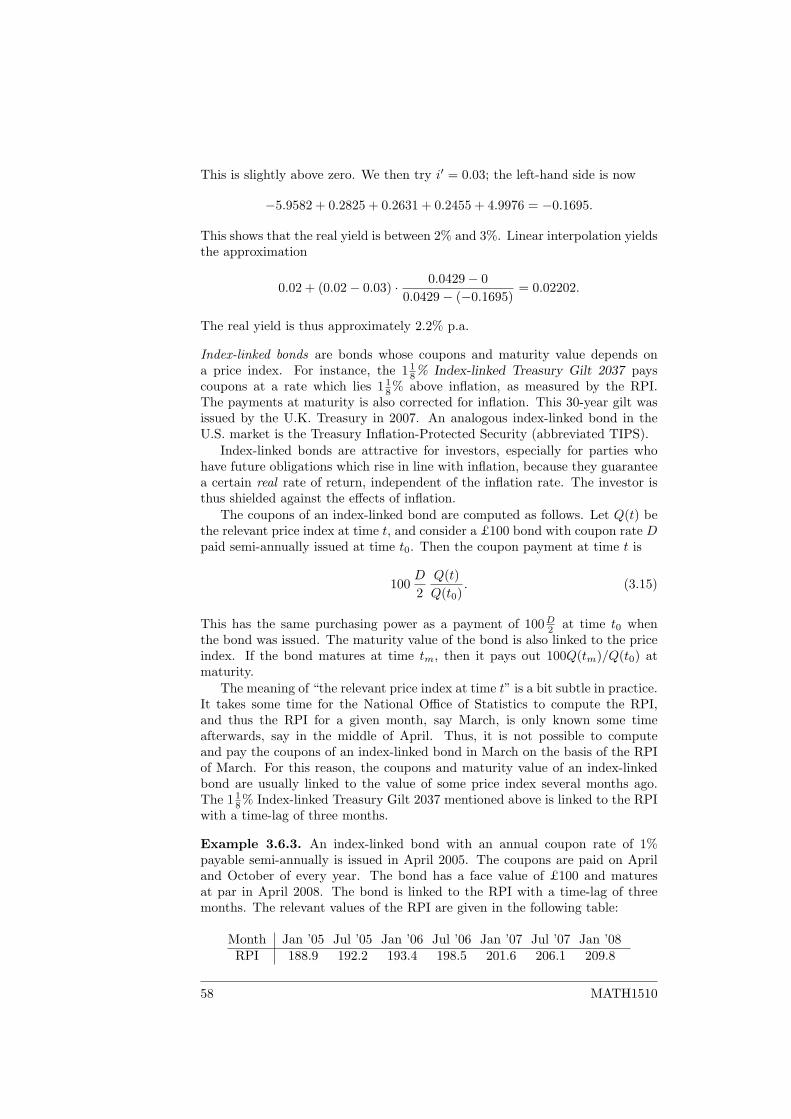
This is slightly above zero. We then try i′ = 0.03; the left-hand side is now

−5.9582 + 0.2825 + 0.2631 + 0.2455 + 4.9976 = −0.1695.

This shows that the real yield is between 2% and 3%. Linear interpolation yieldsthe approximation

0.02 + (0.02− 0.03) · 0.0429− 00.0429− (−0.1695)

= 0.02202.

The real yield is thus approximately 2.2% p.a.

Index-linked bonds are bonds whose coupons and maturity value depends ona price index. For instance, the 1 1

8% Index-linked Treasury Gilt 2037 payscoupons at a rate which lies 1 1

8% above inflation, as measured by the RPI.The payments at maturity is also corrected for inflation. This 30-year gilt wasissued by the U.K. Treasury in 2007. An analogous index-linked bond in theU.S. market is the Treasury Inflation-Protected Security (abbreviated TIPS).

Index-linked bonds are attractive for investors, especially for parties whohave future obligations which rise in line with inflation, because they guaranteea certain real rate of return, independent of the inflation rate. The investor isthus shielded against the effects of inflation.

The coupons of an index-linked bond are computed as follows. Let Q(t) bethe relevant price index at time t, and consider a £100 bond with coupon rate Dpaid semi-annually issued at time t0. Then the coupon payment at time t is

100D

2Q(t)Q(t0)

. (3.15)

This has the same purchasing power as a payment of 100D2 at time t0 whenthe bond was issued. The maturity value of the bond is also linked to the priceindex. If the bond matures at time tm, then it pays out 100Q(tm)/Q(t0) atmaturity.

The meaning of “the relevant price index at time t” is a bit subtle in practice.It takes some time for the National Office of Statistics to compute the RPI,and thus the RPI for a given month, say March, is only known some timeafterwards, say in the middle of April. Thus, it is not possible to computeand pay the coupons of an index-linked bond in March on the basis of the RPIof March. For this reason, the coupons and maturity value of an index-linkedbond are usually linked to the value of some price index several months ago.The 1 1

8% Index-linked Treasury Gilt 2037 mentioned above is linked to the RPIwith a time-lag of three months.

Example 3.6.3. An index-linked bond with an annual coupon rate of 1%payable semi-annually is issued in April 2005. The coupons are paid on Apriland October of every year. The bond has a face value of £100 and maturesat par in April 2008. The bond is linked to the RPI with a time-lag of threemonths. The relevant values of the RPI are given in the following table:

Month Jan ’05 Jul ’05 Jan ’06 Jul ’06 Jan ’07 Jul ’07 Jan ’08RPI 188.9 192.2 193.4 198.5 201.6 206.1 209.8

58 MATH1510

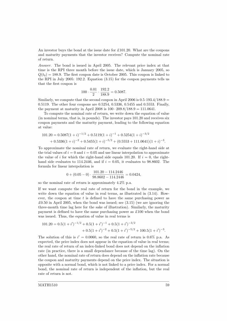
An investor buys the bond at the issue date for £101.20. What are the couponsand maturity payments that the investor receives? Compute the nominal rateof return.

Answer. The bond is issued in April 2005. The relevant price index at thattime is the RPI three month before the issue date, which is January 2005, soQ(t0) = 188.9. The first coupon date is October 2005. This coupon is linked tothe RPI in July 2005: 192.2. Equation (3.15) for the coupon payments tells usthat the first coupon is

100 · 0.012· 192.2

188.9= 0.5087.

Similarly, we compute that the second coupon in April 2006 is 0.5·193.4/188.9 =0.5119. The other four coupons are 0.5254, 0.5336, 0.5455 and 0.5553. Finally,the payment at maturity in April 2008 is 100 · 209.8/188.9 = 111.0641.

To compute the nominal rate of return, we write down the equation of value(in nominal terms, that is, in pounds). The investor pays 101.20 and receives sixcoupon payments and the maturity payment, leading to the following equationat value:

101.20 = 0.5087(1 + i)−1/2 + 0.5119(1 + i)−1 + 0.5254(1 + i)−3/2

+ 0.5336(1 + i)−2 + 0.5455(1 + i)−5/2 + (0.5553 + 111.0641)(1 + i)−3.

To approximate the nominal rate of return, we evaluate the right-hand side atthe trial values of i = 0 and i = 0.05 and use linear interpolation to approximatethe value of i for which the right-hand side equals 101.20. If i = 0, the right-hand side evaluates to 114.2446, and if i = 0.05, it evaluates to 98.8602. Theformula for linear interpolation is

0 + (0.05− 0) · 101.20− 114.244698.8602− 114.2446

= 0.0424,

so the nominal rate of return is approximately 4.2% p.a.

If we want compute the real rate of return for the bond in the example, wewrite down the equation of value in real terms, as illustrated in (3.14). How-ever, the coupon at time t is defined to have the same purchasing power as£0.50 in April 2005, when the bond was issued; see (3.15) (we are ignoring thethree-month time lag here for the sake of illustration). Similarly, the maturitypayment is defined to have the same purchasing power as £100 when the bondwas issued. Thus, the equation of value in real terms is

101.20 = 0.5(1 + i′)−1/2 + 0.5(1 + i′)−1 + 0.5(1 + i′)−3/2

+ 0.5(1 + i′)−2 + 0.5(1 + i′)−5/2 + 100.5(1 + i′)−3.

The solution of this is i′ = 0.0060, so the real rate of return is 0.6% p.a. Asexpected, the price index does not appear in the equation of value in real terms;the real rate of return of an index-linked bond does not depend on the inflationrate (in practice, there is a small dependance because of the time lag). On theother hand, the nominal rate of return does depend on the inflation rate becausethe coupon and maturity payments depend on the price index. The situation isopposite with a normal bond, which is not linked to a price index. For a normalbond, the nominal rate of return is independent of the inflation, but the realrate of return is not.

MATH1510 59

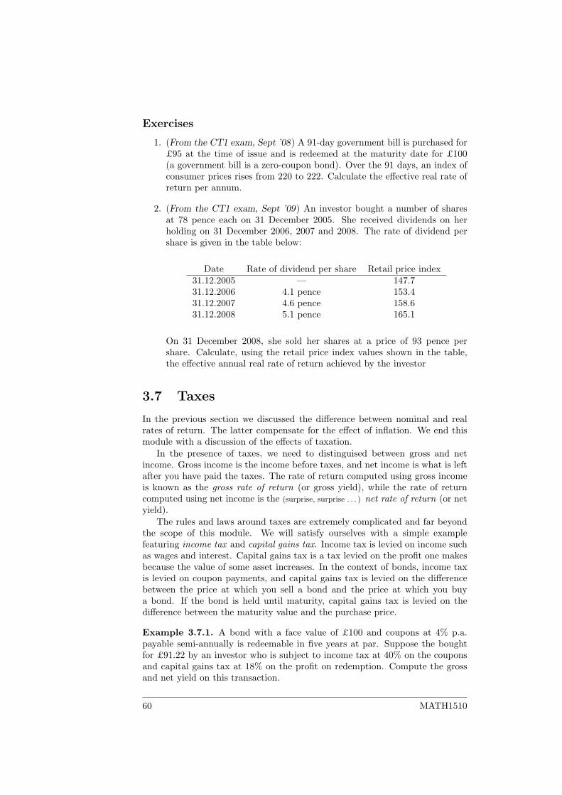
Exercises

1. (From the CT1 exam, Sept ’08) A 91-day government bill is purchased for£95 at the time of issue and is redeemed at the maturity date for £100(a government bill is a zero-coupon bond). Over the 91 days, an index ofconsumer prices rises from 220 to 222. Calculate the effective real rate ofreturn per annum.

2. (From the CT1 exam, Sept ’09) An investor bought a number of sharesat 78 pence each on 31 December 2005. She received dividends on herholding on 31 December 2006, 2007 and 2008. The rate of dividend pershare is given in the table below:

Date Rate of dividend per share Retail price index31.12.2005 — 147.731.12.2006 4.1 pence 153.431.12.2007 4.6 pence 158.631.12.2008 5.1 pence 165.1

On 31 December 2008, she sold her shares at a price of 93 pence pershare. Calculate, using the retail price index values shown in the table,the effective annual real rate of return achieved by the investor

3.7 Taxes

In the previous section we discussed the difference between nominal and realrates of return. The latter compensate for the effect of inflation. We end thismodule with a discussion of the effects of taxation.

In the presence of taxes, we need to distinguised between gross and netincome. Gross income is the income before taxes, and net income is what is leftafter you have paid the taxes. The rate of return computed using gross incomeis known as the gross rate of return (or gross yield), while the rate of returncomputed using net income is the (surprise, surprise . . . ) net rate of return (or netyield).

The rules and laws around taxes are extremely complicated and far beyondthe scope of this module. We will satisfy ourselves with a simple examplefeaturing income tax and capital gains tax. Income tax is levied on income suchas wages and interest. Capital gains tax is a tax levied on the profit one makesbecause the value of some asset increases. In the context of bonds, income taxis levied on coupon payments, and capital gains tax is levied on the differencebetween the price at which you sell a bond and the price at which you buya bond. If the bond is held until maturity, capital gains tax is levied on thedifference between the maturity value and the purchase price.

Example 3.7.1. A bond with a face value of £100 and coupons at 4% p.a.payable semi-annually is redeemable in five years at par. Suppose the boughtfor £91.22 by an investor who is subject to income tax at 40% on the couponsand capital gains tax at 18% on the profit on redemption. Compute the grossand net yield on this transaction.

60 MATH1510

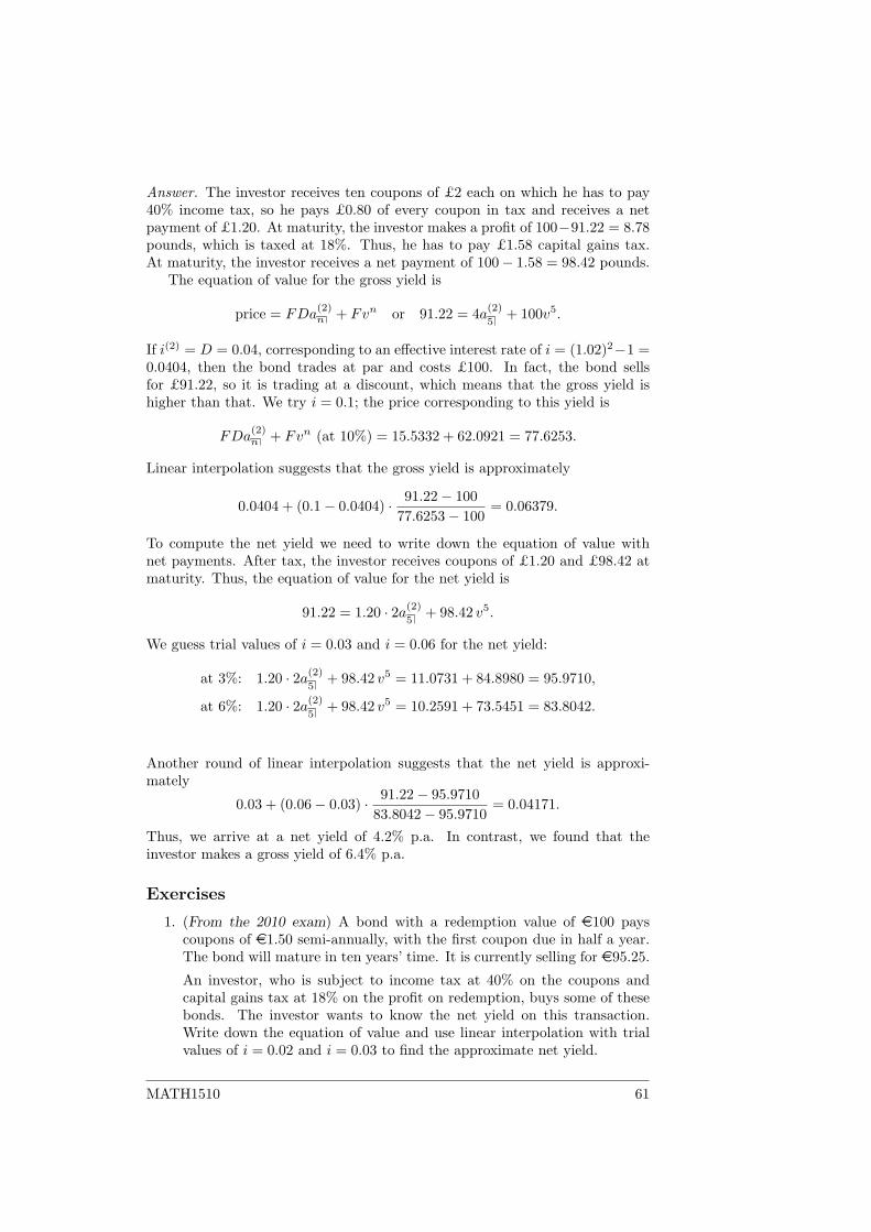
Answer. The investor receives ten coupons of £2 each on which he has to pay40% income tax, so he pays £0.80 of every coupon in tax and receives a netpayment of £1.20. At maturity, the investor makes a profit of 100−91.22 = 8.78pounds, which is taxed at 18%. Thus, he has to pay £1.58 capital gains tax.At maturity, the investor receives a net payment of 100− 1.58 = 98.42 pounds.

The equation of value for the gross yield is

price = FDa(2)n + Fvn or 91.22 = 4a(2)

5+ 100v5.

If i(2) = D = 0.04, corresponding to an effective interest rate of i = (1.02)2−1 =0.0404, then the bond trades at par and costs £100. In fact, the bond sellsfor £91.22, so it is trading at a discount, which means that the gross yield ishigher than that. We try i = 0.1; the price corresponding to this yield is

FDa(2)n + Fvn (at 10%) = 15.5332 + 62.0921 = 77.6253.

Linear interpolation suggests that the gross yield is approximately

0.0404 + (0.1− 0.0404) · 91.22− 10077.6253− 100

= 0.06379.

To compute the net yield we need to write down the equation of value withnet payments. After tax, the investor receives coupons of £1.20 and £98.42 atmaturity. Thus, the equation of value for the net yield is

91.22 = 1.20 · 2a(2)

5+ 98.42 v5.

We guess trial values of i = 0.03 and i = 0.06 for the net yield:

at 3%: 1.20 · 2a(2)

5+ 98.42 v5 = 11.0731 + 84.8980 = 95.9710,

at 6%: 1.20 · 2a(2)

5+ 98.42 v5 = 10.2591 + 73.5451 = 83.8042.

Another round of linear interpolation suggests that the net yield is approxi-mately

0.03 + (0.06− 0.03) · 91.22− 95.971083.8042− 95.9710

= 0.04171.

Thus, we arrive at a net yield of 4.2% p.a. In contrast, we found that theinvestor makes a gross yield of 6.4% p.a.

Exercises

1. (From the 2010 exam) A bond with a redemption value of e100 payscoupons of e1.50 semi-annually, with the first coupon due in half a year.The bond will mature in ten years’ time. It is currently selling for e95.25.

An investor, who is subject to income tax at 40% on the coupons andcapital gains tax at 18% on the profit on redemption, buys some of thesebonds. The investor wants to know the net yield on this transaction.Write down the equation of value and use linear interpolation with trialvalues of i = 0.02 and i = 0.03 to find the approximate net yield.

MATH1510 61

2. (From the sample exam) A bond with a face value of £100 has just beenissued. The bond pays half-yearly coupons of 5% per annum (payablesemi-annually) in arrear and is redeemable at par 20 years after issue.

(a) Without any computations, explain why an investor who wants toachieve a (gross) yield of 6% p.a. should pay less than £100 for thebond.

(b) Assume that the investor pays tax at a rate of 20% on income andis not subject to capital gains tax. Calculate the price to provide aninvestor with a net redemption yield of 6% per annum.

(c) Write down the equation of value for the annual effective gross re-demption yield of this bond assuming the price calculated in ques-tion (b) is paid, and use linear interpolation with trial values of 5%and 6% to compute the gross redemption yield.

(d) Determine the real annual effective gross redemption yield on thisbond if the rate of inflation is constant over the twenty years at 3%per annum.

3. (From the CT1 exam, Sept ’08) A tax advisor is assisting a client inchoosing between three types of investment. The client pays tax at 40%on income and 40% on capital gains.

Investment A requires the investment of £1m and provides an income of£0.1m per year in arrears for ten years. Income tax is deducted at source.At the end of the ten years, the investment of £1m is returned.

In Investment B, the initial sum of £1m accumulates at the rate of 10%per annum compound for ten years. At the end of the ten years, the accu-mulated value of the investment is returned to the investor after deductionof capital gains tax.

Investment C is identical to Investment B except that the initial sumis deemed, for tax purposes, to have increased in line with the index ofconsumer prices between the date of the investment and the end of theten-year period. The index of consumer prices is expected to increase by4% per annum compound over the period.

(a) Calculate the net rate of return expected from each of the invest-ments.

(b) Explain why the expected rate of return is higher for InvestmentC than for Investment B and is higher for Investment B than forInvestment A.

4. (From the CT1 exam, April ’09) A loan pays coupons of 11% per annumquarterly on 1 January, 1 April, 1 July and 1 October each year. Theloan will be redeemed at 115% on any 1 January from 1 January 2015 to1 January 2020 inclusive, at the option of the borrower. In addition tothe redemption proceeds, the coupon then due is also paid.

An investor purchased a holding of the loan on 1 January 2005, immedi-ately after the payment of the coupon then due, at a price which gave hima net redemption yield of at least 8% per annum effective. The investorpays tax at 30% on income and 25% on capital gains.

62 MATH1510

On 1 January 2008 the investor sold the holding, immediately after thepayment of the coupon then due, to a fund which pays no tax. The saleprice gave the fund a gross redemption yield of at least 9% per annumeffective.

Calculate the following:

(a) The price per £100 nominal at which the investor bought the loan.

(b) The price per £100 nominal at which the investor sold the loan.

(c) The net yield per annum convertible quarterly that was actually ob-tained by the investor during the period of ownership of the loan.

MATH1510 63

64 MATH1510

Chapter 4

Payment streams andvariable interest rates

In this chapter we consider two extensions of the theory. Firstly, we look atpayment streams. A payment stream is a payment that occurs continuously,just like the stream of water out of a tap. We model this as the limit of the fol-lowing sequence: annual payments, monthly payments, weekly payments, dailypayments, hourly payments, payments every minute, payments every second,et cetera. Mathematically speaking, we are taking the limit p→∞.

Secondly, we look at variable interest rates. In combination with continuouspayment streams, this give us the most general framework for cash flows. Thisis used in second- and third-year finance modules to price complicated financialinstruments like options.

4.1 The force of interest

A long time ago, in Example 1.5.3, we computed that a nominal rate of 8% p.a.payable quarterly corresponds to an effective rate of 8.243% p.a. As shown inFigure 1.4, this means that a series of four payments of 2 each at the end of everyquarter is equivalent to a single payment of 8.243 at the end of the year. Theother results in Example 1.5.3 show that a series of twelve payments of 8

12 = 23

each at the end of every month is equivalent to a single payment of 8.300 atthe end of the year, that a series of 52 payments of 8

52 each at the end of everyweek is equivalent to a single payment of 8.322 at the end of the year, andthat a series of 365 payments of 8

365 each at the end of every day equivalent toa single payment of 8.328 at the end of the year. More generally, a series ofp payments of i(p)/p each at the end of every period of 1/p year equivalent to asingle payment of

i =(

1 +i(p)

p

)p− 1.

at the end of the year. As the conversion period gets shorter, p gets larger,and it looks like the effective rate tends to a limiting value. In the limit, theinterest is paid continuously. Although this is essentially a theoretical concept,

MATH1510 65

it is important both for conceptual reasons and as an approximation for whenthe conversion period is short.

To study this limit, we fix the effective interest rate i and let p go to infinity.Remember that the nominal rate i(p) is given by

i(p) = p(

(1 + i)1/p − 1). (4.1)

We want to compute the limit of this quantity as p → ∞. To this end, weintroduce h = 1/p, the length of the period between two interest payments (p isthe number of interest payments per year). Substituting this in (4.1), we find

i(1/h) =1h

((1 + i)1/h − 1

).

If p goes to infinity, then h = 1/p goes to zero, so the limit we want to computeis

limp→∞

i(p) = limh→0

i(1/h) = limh→0

(1 + i)1/h − 1h

.

Now comes the smart bit. Recall the definition of the derivative of a function fat a point x0:

dfdx

(x0) = limh→0

f(x0 + h)− f(x0)h.

If we take f(x) = (1 + i)x and x0 = 0, then we get precisely the limit we wantto compute! Turning this around, we find that

limp→∞

i(p) = limh→0

i(1/h) = limh→0

(1 + i)1/h − 1h

=d

dx(1 + i)x|x=0 .

You can get the same result with l’Hopital’s rule for limits, if you know that.However the result is arrived at, we now have to find the derivative of f(x) =(1+i)x. To differentiate this function, rewrite it as f(x) = ex log(1+i), so f ′(x) =log(1 + i) · ex log(1+i) = log(1 + i)(1 + i)x and f ′(0) = log(1 + i). Thus,

limp→∞

i(p) =d

dx(1 + i)x|x=0 = log(1 + i).

We may refer to limp→∞ i(p) as the nominal rate payable continuously, but inpractice another term is used to refer to this quantity.

Definition 4.1.1. The force of interest, denoted δ, is the limit of the nominalinterest rate i(p) as p→∞.

The computation above gives us the relation between the force of interest δ andeffective interest rate i:

δ = log(1 + i). (4.2)

We can also write this relation as i = eδ − 1. If we put δ = 0.08 in here, as inExample 1.5.3, we get i = e0.08−1 = 0.083287. Indeed, the AERs in the answertend to a limiting rate of 8.2387%.

As a side note, if we take the limit p→∞ in (1.5), we get

1 + i = limp→∞

(1 +

δ

p

)p,

66 MATH1510

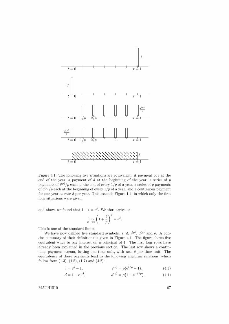
t = 1t = 0

t = 1

i

t = 0

t = 1t = 0

t = 1t = 0 1/p 2/p . . .

t = 1t = 0 1/p 2/p . . .

d

i(p)

p

d(p)

p

δ

Figure 4.1: The following five situations are equivalent: A payment of i at theend of the year, a payment of d at the beginning of the year, a series of ppayments of i(p)/p each at the end of every 1/p of a year, a series of p paymentsof d(p)/p each at the beginning of every 1/p of a year, and a continuous paymentfor one year at rate δ per year. This extends Figure 1.4, in which only the firstfour situations were given.

and above we found that 1 + i = eδ. We thus arrive at

limp→∞

(1 +

δ

p

)p= eδ.

This is one of the standard limits.We have now defined five standard symbols: i, d, i(p), d(p) and δ. A con-

cise summary of their definitions is given in Figure 4.1. The figure shows fiveequivalent ways to pay interest on a principal of 1. The first four rows havealready been explained in the previous section. The last row shows a contin-uous payment stream, lasting one time unit, with rate δ per time unit. Theequivalence of these payments lead to the following algebraic relations, whichfollow from (1.3), (1.5), (1.7) and (4.2):

i = eδ − 1, i(p) = p(eδ/p − 1

), (4.3)

d = 1− e−δ, d(p) = p(1− e−δ/p

). (4.4)

MATH1510 67

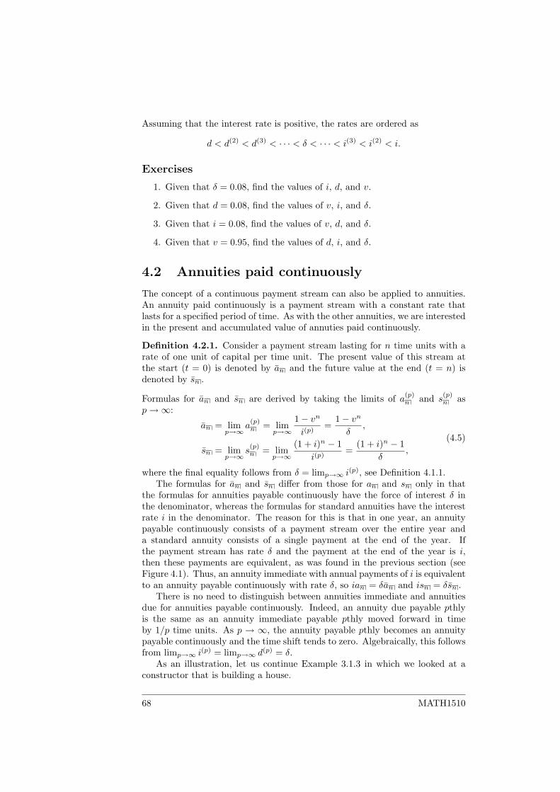
Assuming that the interest rate is positive, the rates are ordered as

d < d(2) < d(3) < · · · < δ < · · · < i(3) < i(2) < i.

Exercises

1. Given that δ = 0.08, find the values of i, d, and v.

2. Given that d = 0.08, find the values of v, i, and δ.

3. Given that i = 0.08, find the values of v, d, and δ.

4. Given that v = 0.95, find the values of d, i, and δ.

4.2 Annuities paid continuously

The concept of a continuous payment stream can also be applied to annuities.An annuity paid continuously is a payment stream with a constant rate thatlasts for a specified period of time. As with the other annuities, we are interestedin the present and accumulated value of annuties paid continuously.

Definition 4.2.1. Consider a payment stream lasting for n time units with arate of one unit of capital per time unit. The present value of this stream atthe start (t = 0) is denoted by an and the future value at the end (t = n) isdenoted by sn .

Formulas for an and sn are derived by taking the limits of a(p)n and s

(p)n as

p→∞:

an = limp→∞

a(p)n = lim

p→∞

1− vn

i(p)=

1− vn

δ,

sn = limp→∞

s(p)n = lim

p→∞

(1 + i)n − 1i(p)

=(1 + i)n − 1

δ,

(4.5)

where the final equality follows from δ = limp→∞ i(p), see Definition 4.1.1.The formulas for an and sn differ from those for an and sn only in that

the formulas for annuities payable continuously have the force of interest δ inthe denominator, whereas the formulas for standard annuities have the interestrate i in the denominator. The reason for this is that in one year, an annuitypayable continuously consists of a payment stream over the entire year anda standard annuity consists of a single payment at the end of the year. Ifthe payment stream has rate δ and the payment at the end of the year is i,then these payments are equivalent, as was found in the previous section (seeFigure 4.1). Thus, an annuity immediate with annual payments of i is equivalentto an annuity payable continuously with rate δ, so ian = δan and isn = δsn .

There is no need to distinguish between annuities immediate and annuitiesdue for annuities payable continuously. Indeed, an annuity due payable pthlyis the same as an annuity immediate payable pthly moved forward in timeby 1/p time units. As p → ∞, the annuity payable pthly becomes an annuitypayable continuously and the time shift tends to zero. Algebraically, this followsfrom limp→∞ i(p) = limp→∞ d(p) = δ.

As an illustration, let us continue Example 3.1.3 in which we looked at aconstructor that is building a house.

68 MATH1510

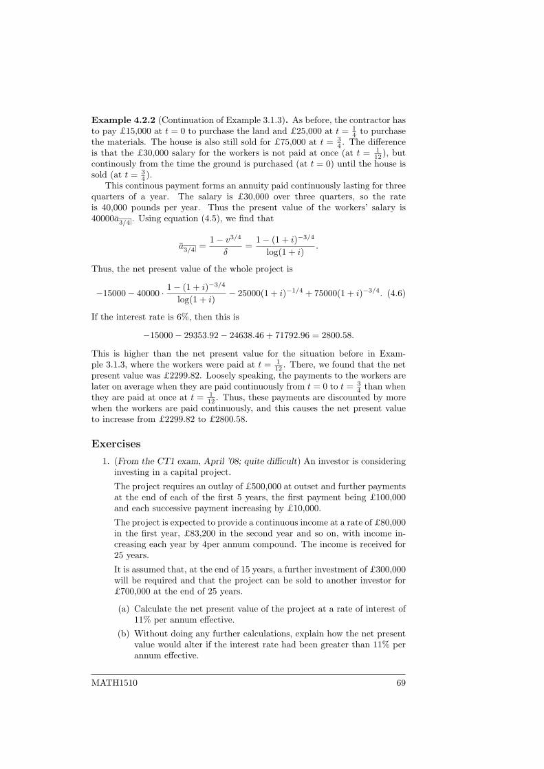
Example 4.2.2 (Continuation of Example 3.1.3). As before, the contractor hasto pay £15,000 at t = 0 to purchase the land and £25,000 at t = 1

4 to purchasethe materials. The house is also still sold for £75,000 at t = 3

4 . The differenceis that the £30,000 salary for the workers is not paid at once (at t = 1

12 ), butcontinously from the time the ground is purchased (at t = 0) until the house issold (at t = 3

4 ).This continous payment forms an annuity paid continuously lasting for three

quarters of a year. The salary is £30,000 over three quarters, so the rateis 40,000 pounds per year. Thus the present value of the workers’ salary is40000a

3/4. Using equation (4.5), we find that

a3/4

=1− v3/4

δ=

1− (1 + i)−3/4

log(1 + i).

Thus, the net present value of the whole project is

−15000− 40000 · 1− (1 + i)−3/4

log(1 + i)− 25000(1 + i)−1/4 + 75000(1 + i)−3/4. (4.6)

If the interest rate is 6%, then this is

−15000− 29353.92− 24638.46 + 71792.96 = 2800.58.

This is higher than the net present value for the situation before in Exam-ple 3.1.3, where the workers were paid at t = 1

12 . There, we found that the netpresent value was £2299.82. Loosely speaking, the payments to the workers arelater on average when they are paid continuously from t = 0 to t = 3

4 than whenthey are paid at once at t = 1

12 . Thus, these payments are discounted by morewhen the workers are paid continuously, and this causes the net present valueto increase from £2299.82 to £2800.58.

Exercises

1. (From the CT1 exam, April ’08; quite difficult) An investor is consideringinvesting in a capital project.

The project requires an outlay of £500,000 at outset and further paymentsat the end of each of the first 5 years, the first payment being £100,000and each successive payment increasing by £10,000.

The project is expected to provide a continuous income at a rate of £80,000in the first year, £83,200 in the second year and so on, with income in-creasing each year by 4per annum compound. The income is received for25 years.

It is assumed that, at the end of 15 years, a further investment of £300,000will be required and that the project can be sold to another investor for£700,000 at the end of 25 years.

(a) Calculate the net present value of the project at a rate of interest of11% per annum effective.

(b) Without doing any further calculations, explain how the net presentvalue would alter if the interest rate had been greater than 11% perannum effective.

MATH1510 69

4.3 Variable interest rates

All the discussion up to now assumes that the interest rate stays constant.However, this is not a realistic assumption. In this section we consider situationsin which the interest rate varies.

We start with a simple example.

Example 4.3.1. Suppose you invest 2000 dollars in an account that pays 4%interest in the first year, 5% in the second year, and 6% in the third year. Howmuch do you have at the end of the third year?

Answer. You have (1+0.04) ·2000 = 2080 dollars after the first year, (1+0.05) ·2080 = 2184 dollars after the second year, and (1+0.06) ·2184 = 2315.04 dollarsafter the third year.

The following computation is not valid: the average rate is 5%, and $2000 at5% over three years accumulates to (1 + 0.05)3 · 2000 = 2315.25 dollars. Indeed,though the result is close to the correct answer, it is not the same.

We now consider a general model which covers the above example, but alsosimple and compound interest with constant rate. The central quantity in thismodel is the accumulation factor.

Definition 4.3.2. The accumulation factor A(t1, t2) is the amount that oneunit of principal at time t1 accumulates to at time t2.

In Example 4.3.1, a principal of $2000 at time t = 0 accumulates to $2080 attime t = 1, so the accumulation factor over this period is A(0, 1) = 2080

2000 = 1.04,corresponding to an interest rate of 4%. Similarly, A(0, 3) = 2315.04

2000 = 1.15752.Two examples are particularly important. The accumulation factor for sim-

ple interest with constant rate i is given by

A(t1, t2) = 1 + i(t2 − t1). (4.7)

The accumulation factor for compound interest with constant rate i is given by

A(t1, t2) = (1 + i)t2−t1 . (4.8)

As we discussed at the end of Section 1.1, simple interest is not consistent inthat you receive less interest if you put money in an account for two years thanif you put money in one account for a year and then take it out with interestand put it in another account for a year. On the other hand, you get the sameamount if compound interest is used. We say that the principle of consistencyholds with compound interest.

Definition 4.3.3. An accumulation function A satisfies the principle of con-sistency if the equation A(t1, t2)A(t2, t3) = A(t1, t3) holds for all values of t1,t2, and t3.

For instance, with compound interest we have:

A(t1, t2)A(t2, t3) = (1 + i)t2−t1 (1 + i)t3−t2 = (1 + i)t3−t1 ,

and

A(t1, t3) = (1 + i)t3−t1 ,

70 MATH1510

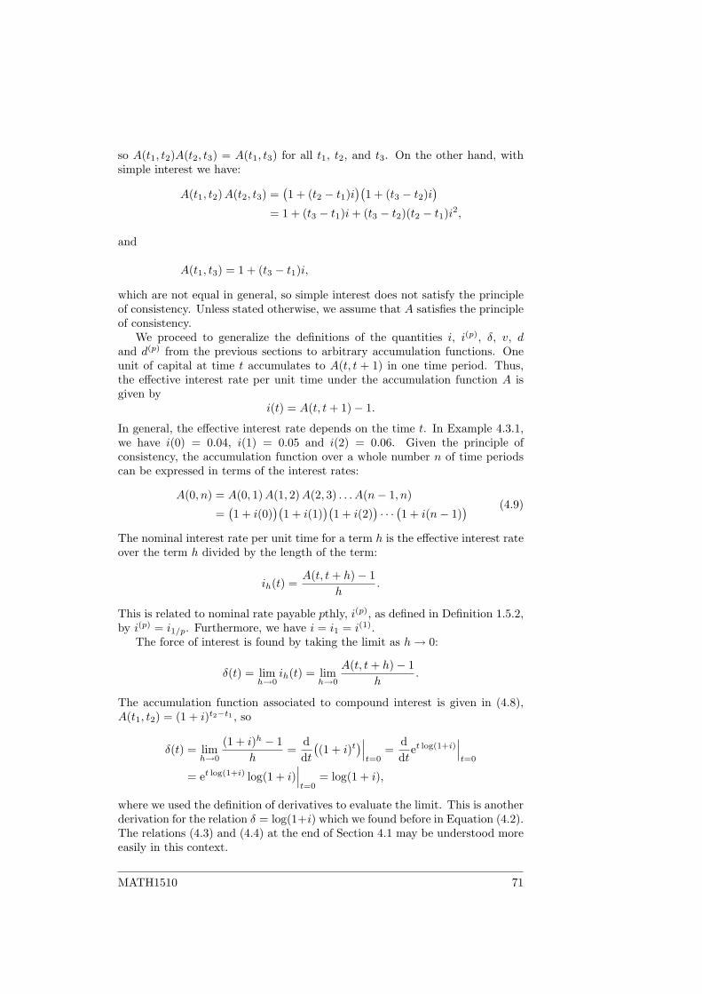
so A(t1, t2)A(t2, t3) = A(t1, t3) for all t1, t2, and t3. On the other hand, withsimple interest we have:

A(t1, t2)A(t2, t3) =(1 + (t2 − t1)i

)(1 + (t3 − t2)i

)= 1 + (t3 − t1)i+ (t3 − t2)(t2 − t1)i2,

and

A(t1, t3) = 1 + (t3 − t1)i,

which are not equal in general, so simple interest does not satisfy the principleof consistency. Unless stated otherwise, we assume that A satisfies the principleof consistency.

We proceed to generalize the definitions of the quantities i, i(p), δ, v, dand d(p) from the previous sections to arbitrary accumulation functions. Oneunit of capital at time t accumulates to A(t, t + 1) in one time period. Thus,the effective interest rate per unit time under the accumulation function A isgiven by

i(t) = A(t, t+ 1)− 1.

In general, the effective interest rate depends on the time t. In Example 4.3.1,we have i(0) = 0.04, i(1) = 0.05 and i(2) = 0.06. Given the principle ofconsistency, the accumulation function over a whole number n of time periodscan be expressed in terms of the interest rates:

A(0, n) = A(0, 1)A(1, 2)A(2, 3) . . . A(n− 1, n)

=(1 + i(0)

)(1 + i(1)

)(1 + i(2)

)· · ·(1 + i(n− 1)

) (4.9)

The nominal interest rate per unit time for a term h is the effective interest rateover the term h divided by the length of the term:

ih(t) =A(t, t+ h)− 1

h.

This is related to nominal rate payable pthly, i(p), as defined in Definition 1.5.2,by i(p) = i1/p. Furthermore, we have i = i1 = i(1).

The force of interest is found by taking the limit as h→ 0:

δ(t) = limh→0

ih(t) = limh→0

A(t, t+ h)− 1h

.

The accumulation function associated to compound interest is given in (4.8),A(t1, t2) = (1 + i)t2−t1 , so

δ(t) = limh→0

(1 + i)h − 1h

=ddt((1 + i)t

)∣∣∣t=0

=ddt

et log(1+i)∣∣∣t=0

= et log(1+i) log(1 + i)∣∣∣t=0

= log(1 + i),

where we used the definition of derivatives to evaluate the limit. This is anotherderivation for the relation δ = log(1+i) which we found before in Equation (4.2).The relations (4.3) and (4.4) at the end of Section 4.1 may be understood moreeasily in this context.

MATH1510 71

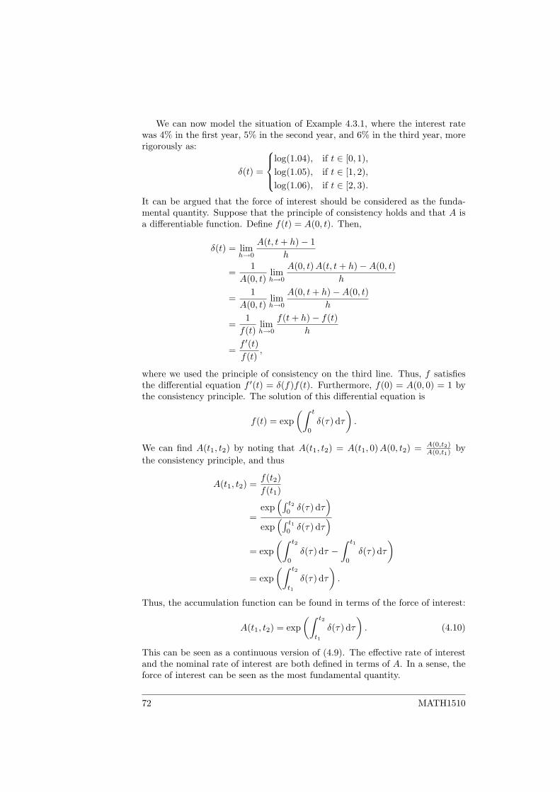
We can now model the situation of Example 4.3.1, where the interest ratewas 4% in the first year, 5% in the second year, and 6% in the third year, morerigorously as:

δ(t) =

log(1.04), if t ∈ [0, 1),log(1.05), if t ∈ [1, 2),log(1.06), if t ∈ [2, 3).

It can be argued that the force of interest should be considered as the funda-mental quantity. Suppose that the principle of consistency holds and that A isa differentiable function. Define f(t) = A(0, t). Then,

δ(t) = limh→0

A(t, t+ h)− 1h

=1

A(0, t)limh→0

A(0, t)A(t, t+ h)−A(0, t)h

=1

A(0, t)limh→0

A(0, t+ h)−A(0, t)h

=1f(t)

limh→0

f(t+ h)− f(t)h

=f ′(t)f(t)

,

where we used the principle of consistency on the third line. Thus, f satisfiesthe differential equation f ′(t) = δ(f)f(t). Furthermore, f(0) = A(0, 0) = 1 bythe consistency principle. The solution of this differential equation is

f(t) = exp(∫ t

0

δ(τ) dτ).

We can find A(t1, t2) by noting that A(t1, t2) = A(t1, 0)A(0, t2) = A(0,t2)A(0,t1)

bythe consistency principle, and thus

A(t1, t2) =f(t2)f(t1)

=exp

(∫ t20δ(τ) dτ

)exp

(∫ t10δ(τ) dτ

)= exp

(∫ t2

0

δ(τ) dτ −∫ t1

0

δ(τ) dτ)

= exp(∫ t2

t1

δ(τ) dτ).

Thus, the accumulation function can be found in terms of the force of interest:

A(t1, t2) = exp(∫ t2

t1

δ(τ) dτ). (4.10)

This can be seen as a continuous version of (4.9). The effective rate of interestand the nominal rate of interest are both defined in terms of A. In a sense, theforce of interest can be seen as the most fundamental quantity.

72 MATH1510

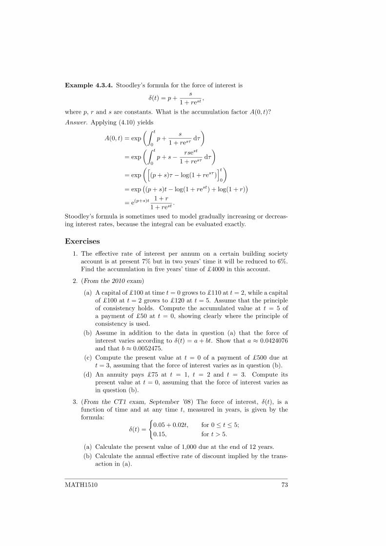
Example 4.3.4. Stoodley’s formula for the force of interest is

δ(t) = p+s

1 + rest,

where p, r and s are constants. What is the accumulation factor A(0, t)?

Answer. Applying (4.10) yields

A(0, t) = exp(∫ t

0

p+s

1 + resτdτ)

= exp(∫ t

0

p+ s− rsest

1 + resτdτ)

= exp([

(p+ s)τ − log(1 + resτ )]t0

)= exp

((p+ s)t− log(1 + rest) + log(1 + r)

)= e(p+s)t 1 + r

1 + rest.

Stoodley’s formula is sometimes used to model gradually increasing or decreas-ing interest rates, because the integral can be evaluated exactly.

Exercises

1. The effective rate of interest per annum on a certain building societyaccount is at present 7% but in two years’ time it will be reduced to 6%.Find the accumulation in five years’ time of £4000 in this account.

2. (From the 2010 exam)

(a) A capital of £100 at time t = 0 grows to £110 at t = 2, while a capitalof £100 at t = 2 grows to £120 at t = 5. Assume that the principleof consistency holds. Compute the accumulated value at t = 5 ofa payment of £50 at t = 0, showing clearly where the principle ofconsistency is used.

(b) Assume in addition to the data in question (a) that the force ofinterest varies according to δ(t) = a + bt. Show that a ≈ 0.0424076and that b ≈ 0.0052475.

(c) Compute the present value at t = 0 of a payment of £500 due att = 3, assuming that the force of interest varies as in question (b).

(d) An annuity pays £75 at t = 1, t = 2 and t = 3. Compute itspresent value at t = 0, assuming that the force of interest varies asin question (b).

3. (From the CT1 exam, September ’08) The force of interest, δ(t), is afunction of time and at any time t, measured in years, is given by theformula:

δ(t) =

{0.05 + 0.02t, for 0 ≤ t ≤ 5;0.15, for t > 5.

(a) Calculate the present value of 1,000 due at the end of 12 years.(b) Calculate the annual effective rate of discount implied by the trans-

action in (a).

MATH1510 73

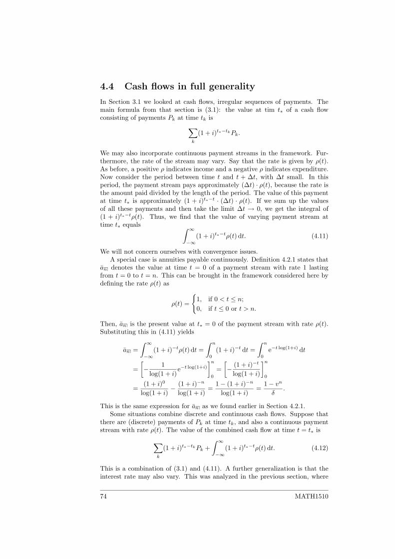
4.4 Cash flows in full generality

In Section 3.1 we looked at cash flows, irregular sequences of payments. Themain formula from that section is (3.1): the value at tim t∗ of a cash flowconsisting of payments Pk at time tk is∑

k

(1 + i)t∗−tkPk.

We may also incorporate continuous payment streams in the framework. Fur-thermore, the rate of the stream may vary. Say that the rate is given by ρ(t).As before, a positive ρ indicates income and a negative ρ indicates expenditure.Now consider the period between time t and t + ∆t, with ∆t small. In thisperiod, the payment stream pays approximately (∆t) · ρ(t), because the rate isthe amount paid divided by the length of the period. The value of this paymentat time t∗ is approximately (1 + i)t∗−t · (∆t) · ρ(t). If we sum up the valuesof all these payments and then take the limit ∆t → 0, we get the integral of(1 + i)t∗−tρ(t). Thus, we find that the value of varying payment stream attime t∗ equals ∫ ∞

−∞(1 + i)t∗−tρ(t) dt. (4.11)

We will not concern ourselves with convergence issues.A special case is annuities payable continuously. Definition 4.2.1 states that

an denotes the value at time t = 0 of a payment stream with rate 1 lastingfrom t = 0 to t = n. This can be brought in the framework considered here bydefining the rate ρ(t) as

ρ(t) =

{1, if 0 < t ≤ n;0, if t ≤ 0 or t > n.

Then, an is the present value at t∗ = 0 of the payment stream with rate ρ(t).Substituting this in (4.11) yields

an =∫ ∞−∞

(1 + i)−tρ(t) dt =∫ n

0

(1 + i)−t dt =∫ n

0

e−t log(1+i) dt

=[− 1

log(1 + i)e−t log(1+i)

]n0

=[− (1 + i)−t

log(1 + i)

]n0

=(1 + i)0

log(1 + i)− (1 + i)−n

log(1 + i)=

1− (1 + i)−n

log(1 + i)=

1− vn

δ.

This is the same expression for an as we found earlier in Section 4.2.1.Some situations combine discrete and continuous cash flows. Suppose that

there are (discrete) payments of Pk at time tk, and also a continuous paymentstream with rate ρ(t). The value of the combined cash flow at time t = t∗ is∑

k

(1 + i)t∗−tkPk +∫ ∞−∞

(1 + i)t∗−tρ(t) dt. (4.12)

This is a combination of (3.1) and (4.11). A further generalization is that theinterest rate may also vary. This was analyzed in the previous section, where

74 MATH1510

we introduced the accumulation function A(t1, t2). The value of the combineddiscrete/continuous cash flow in this setting is

PkA(tk, t∗) +∫ ∞−∞

ρ(t)A(t, t∗) dt.

Compound interest with a constant interest rate i has accumulation functionA(t1, t2) = (1 + i)t2−t1 , and substitution of this in the formula above re-trieves (4.12).

Exercises

1. (From the CT1 exam, April ’08) The force of interest, δ(t), is a functionof time and at any time t, measured in years, is given by the formula:

δ(t) =

0.06, 0 ≤ t ≤ 4;0.10− 0.01t 4 < t ≤ 7;0.01t− 0.04 7 < t.

(a) Calculate the value at time t = 5 of £1,000 due for payment at timet = 10.

(b) Calculate the constant rate of interest per annum convertible monthlywhich leads to the same result as in (a) being obtained.

(c) Calculate the accumulated amount at time t = 12 of a paymentstream, paid continuously from time t = 0 to t = 4, under which therate of payment at time t is ρ(t) = 100e0.02t.

Success with the exam!!!

MATH1510 75