i

Anna T. HamiltonCandidate

BiologyDepartment

This dissertation is approved, and it is acceptable in quality and form for publication:

Approved by the Dissertation Committee:

Clifford Dahm, Advisor

Rebecca Bixby

Scott Collins

Laura Crossey

Gerald Z. Jacobi

Bernard Sweeney (outside reader)

ii

THE EFFECTS OF CLIMATE CHANGE ON STREAM INVERTEBRATES IN THEIRROLE AS BIOLOGICAL INDICATORS AND RESPONDERS TO DISTURBANCE

by

Anna T. Hamilton

B.A., Biology, The Johns Hopkins University, 1974M.S., Aquatic Biology, Towson State University, 1983

DISSERTATION

Submitted in Partial Fulfillment of theRequirements for the Degree of

Doctor of PhilosophyBiology

University of New MexicoAlbuquerque, New Mexico

July 2013

iii

ACKNOWLEDGEMENTS

I would like to thank my committee members, Dr. Cliff Dahm, Dr. Becky Bixby, Dr.

Scott Collins, Dr. Laura Crossey, Dr. Jerry Jacobi, and Dr. Bernard Sweeney (outside

reader) for professional guidance and ongoing support during this project. I would like to

acknowledge Dr. Britta Bierwagen at the U.S. EPA Global Charge Research Program,

and Jen Stamp and Dr. Michael Barbour at the Tetra Tech, Inc. Center for Ecological

Sciences, for their invaluable inputs and close collaboration in the development and

execution of this project. I would like to acknowledge Dr. Bob Parmenter and Scott

Compton of the Valles Caldera National Preserve (VCNP) for providing access to the

study site and site-specific data. I also would like to thank Betsy Shafer, Lauren Sherson,

Susan Kutvirt, Virginia Thompson, Jennifer Clark, Alex Clark, John Craig, Dave Van

Horn, and Jesus Gomez for field, laboratory, and/or data assistance in execution of the

Valles Caldera study. I would especially like to thank my husband, David Hamilton, for

the strong and ongoing intellectual and emotional support he provided throughout this

project.

Funding for the study of the effects of climate change on stream invertebrates in

their role as biological indicators (Chapters 2 and 3) was provided by the U.S. EPA

Global Change Research Program, within the National Center for Environmental

Assessment, Office of Research and Development, under Contract No.GS-10F-0268K,

U.S. EPA Order No. 1107 to Tetra Tech, Inc.. Funding for the study of fire effects in the

VCNP was provided by the New Mexico Experimental Program to Stimulate

Competitive Research (NM EPSCoR). Support for Anna Hamilton was also provided by

Tetra Tech, Inc. Center for Ecological Sciences.

iv

THE EFFECTS OF CLIMATE CHANGE ON STREAM INVERTEBRATES IN THEIRROLE AS BIOLOGICAL INDICATORS AND RESPONDERS TO DISTURBANCE

by

Anna T. Hamilton

B.A., Biology, The Johns Hopkins University, 1974M.S., Aquatic Biology, Towson State University, 1983

DISSERTATIONSubmitted in Partial Fulfillment of the

Requirements for the Degree of

Doctor of PhilosophyBiology

ABSTRACT

Global climate models provide estimates of future changes in air temperature and

precipitation patterns, drought, flooding, sea-level rise, and increases in the frequency,

duration, and intensity of extreme heat and storm events. These climate changes will

affect stream invertebrate communities directly, indirectly, and through interactions with

other stressors, resulting in a range of biological responses, including species range shifts,

losses and replacements, novel community compositions, and altered ecosystem

functions and services. Effects will vary regionally and present heretofore unaccounted

influences on biomonitoring, which water-quality agencies use to assess the status and

health of ecosystems as required by the Clean Water Act. Biomonitoring uses biological

indicators and metrics to assess ecosystem condition, and is anchored in comparison of

test sites to regionally established reference benchmarks of ecological condition. Climate

change will affect responses and interpretation of these indicators and metrics at both

reference and non-reference sites and, therefore, has the potential to confound the

v

diagnosis of ecological condition if reference and non-reference sites do not change in

parallel. This dissertation analyzes four regionally distributed state biomonitoring data

sets to inform on 1) how biological indicators respond to the effects of climate change, 2)

what climate-specific indicators may be available to detect effects, 3) how well current

sampling detects climate-driven changes, and 4) how program designs can continue to

detect impairment. In addition, responses were examined of stream invertebrates to a

particular extreme event, wildfire, which is expected to increase in the future with climate

change.

In general, we found that temperature trait groups (cold- and warm-water

preference taxa), as well as several taxonomically-defined invertebrate metrics and

indicator groups, show responses consistent with expectation to long-term increases in

temperature, although the climate responsiveness of these trait groups varied among

states and ecoregions. Temperature sensitivity of taxa and their sensitivity to organic

pollution were moderately but significantly correlated. Therefore, metrics selected for

condition assessments because taxa are sensitive to disturbance or to conventional

pollutants also were sensitive to changes in temperature. We explored the feasibility of

modifying metrics by partitioning components based on temperature sensitivity to reduce

the likelihood that responses to climate change would confound the interpretation of

responses to impairment from other causes and to facilitate tracking of climate-change-

related taxon losses and replacements. Difficulties arise in categorizing unique indicators

of global changes, because of similarities in some of the temperature and hydrologic

effects resulting from climate change, land use changes, and water removal.

Nevertheless, the utilization of climate-sensitive traits to modify traditional

vi

biomonitoring metrics is promising in the context of using a weight-of-evidence approach

for interpreting bioassessment results. Observed invertebrate responses to climate change

also impair the condition of reference stations. Combined with our projection that

encroachment of developed land uses over time will negatively impact up to a third or

more of currently established reference sites by the end of the century, these responses

suggest the importance of accounting for reference condition drift through

implementation of an objective scale for condition characterization, as well as the need

for reference station protection.

These results can be used to identify methods that assist with detecting climate-

related effects and highlight steps that can be taken to ensure that programs continue to

meet resource protection goals. However, we also must recognize that many aspects of

global changes are not tractable at the local to regional scales at which bioassessment is

applied in support of water quality management, suggesting the need for a shift in the

scale of approach from a narrow focus in the process of water resource quality protection

and restoration to one that encompasses broader adaption strategies to address and

manage global change impacts.

Overall, we found the response of stream benthic invertebrates to a major wildfire

were not devastating, with minimal responses found in total abundance or taxa richness.

However, numerous taxa responded to post-fire flow and water quality disturbances

either positively, negatively, negatively with recovery, or neutrally, with responses well

captured by selected habit and feeding type traits. Post-fire benthic responses reflected

three categories, vulnerability, resistance, and resilience, with different groups of

organisms and different trait characteristics comprising each. Vulnerability was observed

vii

to both direct physical disturbance, mediated by the flow pulses that followed the fire;

and to trophic impacts, themselves a response to loss of food resources due to those same

flow pulses and associated water quality effects. Resistance to the post-fire physical

disturbance of the stream environment was exhibited by a subset of invertebrates with

habit traits that conferred the ability to withstand dislodgement and displacement that

would otherwise be expected from the post-fire flow pulses. Resilience, or ability to

recover in the short term following cessation of the most prominent post-fire flow events,

was conferred mainly by opportunistic life-history traits. This suite of responses suggest

the mechanisms through which benthic communities may be altered in the long-term,

through suppression of some vulnerable taxa, partial if not temporary (short-term)

suppression of some trophic resources, and possibly incomplete recovery (relative to pre-

fire conditions) based on the reproductive life-history characteristics of component taxa.

viii

TABLE OF CONTENTS

CHAPTER 1

INTRODUCTION

Climate Change Context .................................................................................................... 1

Bioassessment Context ...................................................................................................... 6

Vulnerability of Metrics and Indices to Climate Change .................................................. 9

Linkages to Water Law, Stream Management, and Regulation ...................................... 12

Linkages to an Extreme Event – Fire............................................................................... 13

CHAPTER 2

Vulnerability of biological metrics and MMIs to effects of climate change

(Anna T. Hamilton, Jennifer D. Stamp, and Britta G. Bierwagen)

CHAPTER 2 ABSTRACT ............................................................................................. 16

CHAPTER 2 INTRODUCTION.................................................................................... 18

CHAPTER 2 METHODS............................................................................................... 21

State biomonitoring data sets ...................................................................................... 21

Sites used for analysis................................................................................................. 22

Data management........................................................................................................ 24

Temperature and year trend analysis .......................................................................... 25

Responses of commonly used metrics ........................................................................ 26

MMI vulnerabilities .................................................................................................... 27

Modified metrics using temperature-preference traits ................................................ 28

CHAPTER 2 RESULTS.................................................................................................. 30

Temperature and year trend analysis .......................................................................... 30

ix

Responses of commonly used metrics and MMI vulnerabilities ................................ 33

Modified metrics using temperature-preference traits ................................................ 41

CHAPTER 2 DISCUSSION .......................................................................................... 43

Interactive effects of ecoregional characteristics and climate change on

bioassessment metrics................................................................................................. 43

Responses of commonly used metrics and MMI vulnerabilities ................................ 45

Modified metrics using temperature-preference traits ................................................ 47

Potential effects of losses of cold-water-preference taxa on MMI-based assessments49

Limitations .................................................................................................................. 51

CHAPTER 2 LITERATURE CITED............................................................................. 55

CHAPTER 2 APPENDIX .............................................................................................. 61

CHAPTER 3

Implications of global change for the maintenance of water quality and ecological

integrity in the context of current water laws and environmental policies

(Anna T. Hamilton, Michael T. Barbour, and Britta G. Bierwagen)

CHAPTER 3 ABSTRACT ............................................................................................. 62

CHAPTER 3 THE UNDERPINNINGS OF ENVIRONMENTAL PROTECTION OF

AQUATIC RESOURCES ............................................................................................... 64

CHAPTER 3 GLOBAL CHANGES AND ECOSYSTEM HEALTH .......................... 68

CHAPTER 3 SUSCEPTIBLE ASPECTS OF ASSESSMENT PROGRAMS TO

GLOBAL CHANGES ..................................................................................................... 72

CHAPTER 3 INTEGRATION OF MONITORING AND ASSESSMENT FOR

GLOBAL CHANGE INTO ENVIRONMENTAL POLICY.......................................... 79

x

What do we do about loss of reference conditions? ................................................... 80

How do we Resolve Mixed Messages from Existing Biological Indicators?............. 85

Why Embrace A Management Paradigm Shift? ......................................................... 88

CHAPTER 3 REFERENCES......................................................................................... 92

CHAPTER 4

Short-Term Effects of the Las Conchas Fire on Benthos in the East Fork Jemez

River in the Valles Caldera, New Mexico

(Anna Hamilton, Clifford N. Dahm, Rebecca J. Bixby, Gerald Z. Jacobi, Betsy M.

Shafer, Lauren Sherson, Virginia F. Thompson, Alexander Clark, Shann M. Stringer)

CHAPTER 4 ABSTRACT ........................................................................................... 101

CHAPTER 4 INTRODUCTION.................................................................................. 102

CHAPTER 4 METHODS............................................................................................. 106

Study Area ................................................................................................................ 106

Water Quality, Chemistry, and Streamflow Measurements ..................................... 108

Biological Sampling.................................................................................................. 109

Data Analysis ............................................................................................................ 111

Classification Techniques .................................................................................... 112

Indicator Species.................................................................................................. 113

Las Conchas Fire....................................................................................................... 114

CHAPTER 4 RESULTS............................................................................................... 115

General EFJR Habitats and Benthic Communities Characteristics .......................... 115

Benthic Invertebrate Trait Responses ....................................................................... 124

Key Species Patterns................................................................................................. 131

xi

CHAPTER 4 DISCUSSION ........................................................................................ 132

Water Quality Responses of the EFJR to the Fire .................................................... 133

Characteristics of the EFJR Benthic Communities................................................... 138

Before and After Sampling of Invertebrates in a Fire-Impacted Stream .................. 141

Functional Trait Responses to the Las Conchas Fire................................................ 145

Short-Term Effects, Long-Term Expectations ......................................................... 149

CHAPTER 4 REFERENCES....................................................................................... 152

CHAPTER 5

Summary

CHAPTER 5 SUMMARY ........................................................................................... 157

CHAPTER 5 REFERENCES....................................................................................... 161

xii

LIST OF FIGURES

CHAPTER 1 Figure 1........................................................................................................ 9

CHAPTER 2 Figure 1...................................................................................................... 32

CHAPTER 2 Figure 2...................................................................................................... 34

CHAPTER 2 Figure 3...................................................................................................... 35

CHAPTER 2 Figure 4...................................................................................................... 38

CHAPTER 2 Figure 5...................................................................................................... 39

CHAPTER 2 Figure 6...................................................................................................... 40

CHAPTER 2 Figure 7...................................................................................................... 41

CHAPTER 2 Figure 8...................................................................................................... 43

CHAPTER 3 Figure 1...................................................................................................... 70

CHAPTER 3 Figure 2...................................................................................................... 74

CHAPTER 3 Figure 3...................................................................................................... 75

CHAPTER 3 Figure 4...................................................................................................... 76

CHAPTER 4 Figure 1.................................................................................................... 107

CHAPTER 4 Figure 2.................................................................................................... 114

CHAPTER 4 Figure 3.................................................................................................... 116

CHAPTER 4 Figure 4.................................................................................................... 118

CHAPTER 4 Figure 5.................................................................................................... 119

CHAPTER 4 Figure 6.................................................................................................... 122

CHAPTER 4 Figure 7.................................................................................................... 125

CHAPTER 4 Figure 8.................................................................................................... 127

CHAPTER 4 Figure 9.................................................................................................... 128

xiii

CHAPTER 4 Figure 10.................................................................................................. 130

CHAPTER 4 Figure 11.................................................................................................. 131

CHAPTER 4 Figure 12.................................................................................................. 132

CHAPTER 4 Figure 13.................................................................................................. 135

CHAPTER 4 Figure 14.................................................................................................. 136

CHAPTER 4 Figure 15.................................................................................................. 136

CHAPTER 4 Figure 16.................................................................................................. 143

xiv

LIST OF TABLES

CHAPTER 2 Table 1 ....................................................................................................... 23

CHAPTER 2 Table 2 ....................................................................................................... 29

CHAPTER 2 Table 3 ....................................................................................................... 31

CHAPTER 3 Table 1 ....................................................................................................... 71

CHAPTER 3 Table 2 ....................................................................................................... 72

CHAPTER 3 Table 3 ....................................................................................................... 82

CHAPTER 4 Table 1 ..................................................................................................... 115

CHAPTER 4 Table 2 ..................................................................................................... 117

CHAPTER 4 Table 3 ..................................................................................................... 119

CHAPTER 4 Table 4 ..................................................................................................... 120

CHAPTER 4 Table 5 ..................................................................................................... 123

CHAPTER 4 Table 6 ..................................................................................................... 123

CHAPTER 4 Table 7 ..................................................................................................... 125

CHAPTER 4 Table 8 ..................................................................................................... 126

CHAPTER 4 Table 9 ..................................................................................................... 127

CHAPTER 4 Table 10 ................................................................................................... 129

1

CHAPTER 1

INTRODUCTION

Climate Change Context

The reality of global climate change is well established (IPCC 2007a, b; NCADAC

2013), if not well perceived by the public (Seacrest et al. 2000). Changing patterns of

climate forcing are expected to alter spatial and temporal patterns of air temperature and

precipitation that in turn will drive changes in sea level rise, ice cover, timing and

magnitude of snow melt, evapotranspiration, drought, flooding magnitude and frequency,

and other extreme events (IPCC 2007a). Many of these global changes will impact people

directly (NCADAC 2013). Climate change impacts to stream and river systems are also a

specific concern for people, because of our dependence on surface waters for water

supply, recreational uses, and ecosystem services, as well as our concerns with

environmental quality, habitat protection, and biodiversity (Palmer et al. 2009).

Projections of climate change patterns for air temperature and precipitation come

from general circulation models (GCMs). These models provide good insight into the

magnitude and scale of changes that will affect the landscapes drained by streams and

thus the structure and function of the streams themselves. Combining the outputs from

numerous GCMs over a range of potential future scenarios for greenhouse gas emissions

provides an ensemble of projected changes in temperature and precipitation patterns

(IPCC 2007a). Global average projections of temperature increase over the current

century by values that range from 1.1−2.9oC for the lowest emissions scenario to 2.4–

6.4oC for the highest (IPCC 2007a). This projected rate of increase is ~53% higher (about

0.2oC per decade) than the rate observed over the last 50 years (0.13oC per decade), and

2

further rate increases are considered possible (IPCC 2007b, Ramstorf et al. 2007, Hansen

et al. 2006). Projections are more uncertain for precipitation (IPCC 2007a), and vary

among major geographic regions of the continental U.S. (e.g., Shoof et al. 2010).

However, general projections include increased frequency of heavy precipitation events,

more precipitation in winter and less precipitation in summer, more winter precipitation

as rain instead of snow, earlier snow-melt, earlier ice-off in rivers and lakes, longer

periods of low flow, and more frequent droughts in summer (IPCC 2007a, Barnett et al.

2005, Hayhoe et al. 2007, Fisher et al. 1997). In some regions, particularly the west and

southwest, other extreme events such as major wildfires are projected to increase in

connection with higher spring and summer temperatures, earlier spring snowmelt, and

increasing aridity (Westerling et al. 2006, Seager et al. 2007).

Changes in air temperature and precipitation are key climate change factors that

will impact stream and river ecosystems through direct effects on water temperature and

hydrologic regimes, as well as through indirect effects on dissolved oxygen (DO), pH,

nutrients, and other dissolved constituents, and changes in the assimilation capacity of

pollutants into receiving waters, sediment erosion and deposition, and habitat structure.

Just as climate patterns and projections for climate change vary among regions of the

U.S. (and globally), effects of climate change on stream systems will also vary

geographically. Stream water temperature patterns closely follow air temperature patterns

(e.g., Mohseni et al. 2003, Pilgrim et al. 1998, Stephan and Preudhomme 1993),

potentially resulting in predictable regional shifts in stream thermal regimes. However,

stream water temperatures are directly driven by solar insolation (rather than air

temperature) and are affected by smaller scale factors that include variations in flow

3

volume and snow melt, ground water influence, aspect, riparian shading, presence of

deep pools, meteorology, river conditions, and geographic setting (e.g., elevation,

gradient, etc.) (Allen and Castillo 2007, Caissie 2006, Mohseni et al. 2003, Daufresne et

al. 2003, Hawkins et al. 1997, Ward 1985). Patterns in changing stream temperatures may

not be predictable without accounting for at least some of these effects. Recent estimates

of ‘climate velocity,’ which relate future projections of change in a climate variable such

as temperature to the spatial gradient in that variable, yield a geographically more

complex set of climate change expectations. These expectations reflect, for example,

more uniform projections of magnitudes and directions of change in the plains of central

and southeastern U.S., and more variable expectations in mountainous regions

(Dobrowski et al. 2012). Nevertheless, changes in the thermal regimes of streams and

rivers in response to climate change have been documented from long-term river

temperature datasets around the country (e.g., Kaushel et al. 2010).

Climate changes also will impact the hydrologic characteristics of streams, with

consequences to stream biological communities (e.g., Webb et al. 2009, Dewson et al.

2007, Suren and Jowett 2006, Lind et al. 2006, Poff 2002, Extence et al. 1999, Stanley et

al. 1994). The IPCC (2007a) projects average annual runoff to increase by 10-40% at

high latitudes and in some tropical areas, but to decrease by 10-30% over some mid-

latitudes dry regions and the dry tropics. In North America, projected changes in average

stream flow range from an increase of 10–40% at high latitudes to a decrease of about

10–30% in mid-latitude western North America by 2050 (Milly et al. 2005). The

hydrologic regime of a stream is not a singular variable, and the range of hydrologic

alterations that can result from the combination of increasing magnitude and variability of

4

temperatures combined with a range of projected changes in precipitation and drought

conditions is great, potentially including longer duration and lower summer low flows,

greater incidence of floods, and greater flashiness. In western/southwestern snow pack

dominated regions, the combination of warming temperatures, a shift toward less winter

precipitation falling as snow, and snow melt occurring earlier will shift the peak runoff

from spring to late-winter/early spring, accompanied by a reduced magnitude of snow

pack (Barnett et al. 2005, Clow 2010). Typical projections are for peak runoff to shift

from about two weeks up to one month earlier by the end of the century (Dettinger et al.

2004, Hayhoe et al. 2007). Stewart et al. (2005) have already found evidence for shifts of

this magnitude (1-4 week earlier timing of snow melt and runoff based on data from 1948

to 2002) for several montane catchments in the western U.S. The effects of water

temperature can also interact with stream flow alterations, with higher temperatures and

higher warming rates during low flow conditions (Vliet and Zwolsman 2008, Zwolsman

and Van Bokhoven 2007, Sinokrot and Gulliver 2000). As a result, influences of stream

temperatures and flow conditions cannot always be separated in terms of their effects on

biota.

Freshwater ecosystems are considered sensitive to climate change impacts because

of their fundamental dependence on hydrology and thermal regimes, their dominance by

poikilotherms, their high degree of isolation and fragmentation within terrestrial systems,

and their vulnerability to impact by humans and further complications via interactions

with other stressors (Isaak and Rieman 2013, Woodward et al. 2010, Durance and

Ormerod 2007). There is growing information on the effects of climate change on aquatic

ecosystems (e.g., Doledec et al. 1996, Durance and Ormerod 2007, Daufresne and Boet

5

2007, Buisson et al. 2008, Hiddink and Hofstede 2008, Collier 2008, Chessman 2009,

Flenner et al. 2010, Britton et al. 2010, Winfield et al. 2010, Floury et al. 2013).

Temperature regimes greatly affect the distribution and abundance of aquatic species and

communities in relation to temperature tolerances and evolutionary adaptations combined

with competitive interactions, effects on food supply, and other factors (e.g., Matthews

1998, Hawkins et al. 1997, Vannote and Sweeney 1980, Sweeney and Vannote 1978).

Changes in prevailing temperature regime, as well as increased variability of temperature

associated with /induced by climate change, may have various biological effects. Species

ranges will shift to the north and/or to higher elevations (Comte and Grenouillet 2013,

Comte et al. 2013); to a lesser extent, species at the southern limits of their ranges may

migrate or suffer local extinctions. Migrations of stream species may be limited by

barriers to dispersal such as habitat fragmentation due to dams and reservoirs,

deforestation, and water diversions (Poff et al. 2002, Moore et al. 1997, Covich et al.

1997, Smith 2004, Hawkins et al. 1997); or in some regions including the Southwest and

southern Great Plains by the prevalence of east-west drainages (Poff et al. 2002). Species

that are already restricted to headwater streams may be displaced (Poff et al. 2002).

Changes in stream flow from climate change may alter community structure through

alteration of quantity and quality of available habitat, as well as through tolerances or

requirements for particular flow conditions. Species replacements, range shifts, and

variations in community composition for both fish and macroinvertebrates have been

documented and associated with increased temperatures and lower flows (Daufresne et al.

2003, Durance and Ormerod 2007, de Figueroa et al. 2010).

6

Bioassessment Context

In the U.S. and in many other countries around the world, environmental protection

regulations such as the U.S. Clean Water Act (CWA) of 1972 identify the restoration and

maintenance of physical, chemical and biological integrity of streams and rivers as a

long-term goal (Barbour et al. 2000). Biological assessment, or ‘bioassessment’, is relied

on as a tool applied by resource managers to achieve this goal (Norris and Barbour 2009).

Bioassessment has been found to be more effective than sampling only chemical

parameters (Karr 2006), largely due to the recognition that biological indicators reflect an

integrated response to all environmental conditions to which they are exposed over time

(Moog and Chovanec 2000, Barbour et al. 2000). Thus, biological indicators can provide

information that may not be revealed by measurement of concentrations of chemical

pollutants or toxicity tests (Barbour et al. 1999, Rosenberg and Resh 1993, Resh and

Rosenberg 1984). Biological assessment, coupled with multi-metric or predictive

modeling analyses, is a strong approach for diagnosing diminished ecological integrity,

minimizing or preventing degradation of river systems (Karr and Chu 2000), and

measuring success of stream and river restoration and mitigation efforts (Palmer et al.

2010).

In the U.S., biological assessment plays a central role in water quality programs that

are components of the CWA, from assessment of water quality and identification of

biologically impaired waters to development of total maximum daily load (TMDL) for

impaired water bodies. Bioassessment results also are used to help identify causes of

observed impairments, based on the assumption that various components of aquatic

communities will respond differently to different types of stressors. Other CWA

7

programs that depend on bioassessment data include permit evaluation and issuance,

tracking responses to restoration actions, and other components of watershed

management and restoration.

Bioassessments rely on characterization of biological indicators and metrics to

assess ecosystem condition, and are grounded in comparisons between reference and non-

reference sites. Climate change, through effects on both reference and non-reference

sites, will impact the responses and interpretation of traditional indicators and metrics,

and has the potential to confound diagnosis of cause for impaired sites not attaining their

aquatic life use. Climate change can confound the interpretation of bioassessment data if

climate changes drive responses in biota that cannot be linked effectively to their climate

change cause, which will be the case in the absence of specific diagnostic efforts which

until recently have been lacking. These could include, for example, development of

climate-sensitive indicators or metrics, or incorporation of long-term sampling for

examination of climate-related trends. Without such focused diagnostic approaches, any

biological responses observed might be attributed to the range of traditional stressors

commonly evaluated. Climate change can further confound the diagnosis of impairment

through climate change-associated degradation of reference sites, making reference sites

more similar to degraded sites and thus more difficult to differentiated statistically

between reference and test conditions, and more difficult to determine degree of

impairment (U.S. EPA 2008).

A variety of biological metrics and indices have been developed as ecological

indicators used to gauge the condition of aquatic ecosystems relative to reference

conditions and to judge causes of degradation (Niemi and McDonald 2004). Indicators

8

are used as early warnings of degradation, as they often simplify complex environmental

data. Various factors govern the selection of biological indicators, including appropriate

spatial and temporal scales, incorporation of natural variability, and sensitivity to the

range of stressors expected in a system (Niemi and McDonald 2004). The concept of

linkage between biological indicators and the stressors on a system is crucial to the

interpretation of bioassessment results. Stream benthic invertebrates are the most

common assemblage used for biomonitoring in this respect (USEPA 2002). Benthic

invertebrates are considered sensitive indicators of their natural environment as well as of

a variety of perturbations. Their integrative characteristics make benthic assemblages

effective monitoring tools, but it also means that all major sources of stress must be

reasonably accounted for in order to reliably attribute observed responses to particular

sources.

Given the evidence of how climate is changing and potentially affecting stream

population and community responses, it is clear the changing influences of such a major

environmental driver should be accounted for in terms of its effects on the components of

bioassessment (Figure 1), all of which can be affected by climate change. This

dissertation and the larger project of which it was a part are among the first to address

many of these concerns, focusing primarily on several of the elements that comprise

assessment design (Figure 1), and applying results to consideration of environmental

management with regard to their implications for decision making. The goals of this work

are to contribute to the foundation for understanding how climate changes affect

bioassessment indicators and for advancing the development of specific strategies to

ensure the long-term effectiveness of monitoring and management plans.

9

Figure 1. Climate change can affect many bioassessment program activities from theinitial assessment design, to collecting and analyzing data, and to developing responses toassessment outcomes (TMDLs = total maximum daily loads).

Vulnerability of Metrics and Indices to Climate Change

The first section of this dissertation (Chapter 2, Hamilton et al. 2010a,

‘Vulnerability of biological metrics and multimetric indices to effects of climate change’)

used several long-term state biomonitoring data sets to investigate 1) whether biological

response signals to climate change are discernible within existing bioassessment datasets;

2) how responses of various biological indicators can be categorized and interpreted with

regard to apparent climate sensitivity or robustness, using both trend analysis and

partitioning of hot and cold years as a proxy for long-term changes in temperature; 3)

whether climate change-sensitive indicators could be developed based on

environmentally realized temperature preferences, and applied to metrics to enhance the

10

ability to differentiate climate change-related influences from the responses to other

stressors; and 4) the vulnerabilities to climate change effects of the metrics and

multimetric indices used to assess impairment to the types of climate change responses

found. Results can be used to identify methods that assist with detecting climate-related

effects and highlight steps that can be taken to ensure that programs continue to meet

resource protection goals.

This chapter of my dissertation is a ‘data mining’ study. The study uses analyses of

existing, long-term biomonitoring datasets, which were collected for another purpose

(i.e., to monitor the status of stream biota using reference-based comparisons) to address

a new question for which the original collection programs were not designed. Global

climate change effects on stream habitats can be seen as long term, progressive changes

overlain on other natural sources of variability, including other climate drivers. While

there are certainly some questions about climate change effects that can be addressed

using spatial comparisons, climate change for the most part is a long-term temporal issue.

Trend analysis is a logical approach to investigate long-term patterns in temperature,

precipitation, flow, other habitat variables, and biological response variables. Trend

analysis forms a foundation for examining evidence that long-term, progressive global

changes are contributing to the trends, and for considering other possible contributions.

Given that in some of the states in the USA there exists biomonitoring programs that

have been in place for long periods of time (e.g., 2+ decades), and that outside of this

arena long-term biological datasets are relatively rare (Jackson and Fureder 2006), it is an

attractive opportunity to apply these long-term biological datasets to the climate change-

related questions that are the focus of this study. This type of post-facto analysis of

11

historical datasets has been used by others to determine whether climate change effects

are already discernible in ecosystem responses (e.g., Daufresne et al. 2003, Durance and

Ormerod 2007, Burgmer et al. 2007, Murphy et al. 2007). However, this data mining

approach has several pitfalls, including the lack of broad spatial coverage by stations with

continuous long-term data, and the lack of long-term data at both reference sites that are

minimally affected by other major anthropogenic stressors as well as stressed sites to help

differentiate related responses. As is often the case with the opportunistic use of mined

data, the existing biomonitoring datasets available for analysis in this study did not

always meet all the criteria that would have allowed the most rigorous evaluation of the

study questions.

Biological responses to climate change are likely to include interactions with

climate cycles such as the Pacific Decadal Oscillation (PDO) or North Atlantic

Oscillation (NAO), which can act synergistically or antagonistically with climate change,

depending on their phases (e.g., Seager and Vecchi 2010). These interactions can

potentially enhance or obscure the types and magnitudes of biological responses that

might be expected over the long term. ‘Climate change’ can be considered the long-term,

average directional changes that span multiple climate cycle oscillations. Nevertheless,

the types, directions, and with caution, the magnitudes of biological responses to climate

change can be inferred from shorter-term (one to two decade) patterns, even in the

absence of the ability to partition long-term direction and cyclic climate patterns. Indeed,

the occurrence of cyclical climate changes provides a set of ‘natural experiments’ that we

can take advantage of to gain insights into what kinds of biological responses can be

expected, and how these will play out with respect to bioassessment. Inference would be

12

based on linkages between changes in climate factors, changes in stream conditions, and

associated changes in biological metrics. This will yield valuable information on the

identification of biological metrics that are sensitive to such climate-associated changes.

It is common practice to infer probable sources of cause by clear associations between

types and sources of stressors present and responses of biota whose autecology

characteristics are known (Norris and Barbour 2009, Cormier and Suter 2008).

Linkages to Water Law, Stream Management, and Regulation

The second section of this dissertation (Chapter 3, Hamilton et al. 2010b,

‘Implications of global change for the maintenance of water quality and ecological

integrity in the context of current water laws and environmental policies’) takes the

results from the studies conducted in Chapter 2 and expands on the evaluation of the

implications of those metric and index responses to the outcomes of decision making for

water resource management. This chapter of the dissertation considers the interactions of

other global change parameters, particularly land use and population growth, in addition

to climate change, with respect to their potential influences on bioassessment metrics and

indices. The chapter also assesses the sensitivities of reference station conditions and

associated impacts to reference-based comparisons that are the foundation of

bioassessment. It compares bioassessment approaches around the world to examine

programmatic vulnerabilities to the combination of global change parameters, and

discerns from this potential programmatic adaptations that could preserve our ultimate

regulatory goals of preserving good water quality and ecological integrity. Awareness

that climate change and other landscape or global-scale stressors can have widespread

13

effects on biological communities introduces additional uncertainty into a system that

assumes there are interpretable patterns of biological indicator responses to

“conventional” stressors. This has the potential to cast doubt on assertions of stressor-

response relationships that are being evaluated within a regulatory context, and also

highlights the potential value of tailoring biomonitoring tools to the types of stressors

expected, as well as accounting for the influences of stressors operating at different

scales. The study also addresses limitations in this objective related to similarities in

biological responses to the sometimes common effects that can arise from different

sources. With increasing knowledge of the types of global change effects that are

appearing to different degrees in regions around the country and the world, and of the

categories of organisms that are showing the most predictable responses, it becomes more

realistic to consider adjusting assessment tools and approaches to account for landscape-

to global-scale stressors through adaptations to existing programs.

Linkages to an Extreme Event - Fire

Stream biological communities change not only in response to long-term shifts in

climate, land use, and other environmental drivers, but also due to the occurrence of

extreme events. Large wildfires are one type of extreme event that not only restructure

terrestrial ecosystems (e.g., Johnson 1992), but also impact the stream ecosystems within

these forested biomes (see Minshall 2003 for a review). Both the frequency (Westerling

et al. 2006) and severity (Miller et al. 2009) of forest fires in the western and

southwestern U.S. are expected to increase with climate change, due to higher spring and

14

summer temperatures and earlier spring snowmelt (Westerling et al. 2006) and the

increasing frequency of drought (Allen 2002).

A study of changes in benthic macroinvertebrates associated with fire provides a

contrast between short-term acute and long-term chronic disturbances, both associated

with human-influenced climate change. Bioassessment approaches are generally attuned

to accounting for short-term influences with identifiable causes. But periodic, though

unpredictable, disturbances will punctuate observed long-term changes, and could alter

the long-term trajectories expected in species and community responses. This component

of the dissertation provides an initial opportunity to characterize the nature of stream

invertebrate responses to an acute, watershed-scale disturbance in terms, such as an

evaluation of responsive traits, which will allow comparison to long-term climate change

responses.

A long-term, well-instrumented study site was established on the East Fork Jemez

River in the Valles Caldera National Preserve in the Jemez Mountains of northern New

Mexico, with the long-term goal of studying climate variability and climate change

impacts on water quantity and quality in a snowmelt-dominated system. It was also a goal

to investigate various ecological linkages with the seasonal dynamics and long-term

variations in water quantity and quality characteristics that were being documented

through sampling of a variety of biological processes and communities including stream

benthic invertebrates. An unexpected but highly valuable opportunity to study the short-

term impact and recovery responses of invertebrates to major wildfire was provided by

the Las Conchas fire, which burned a vast region in the Valles Caldera and the Jemez

Mountains in 2011. The third section of this dissertation (Chapter 4, ‘Short-Term Effects

15

of the Las Conchas Fire on Benthos in the East Fork Jemez River in the Valles Caldera,

New Mexico’) reports on this spontaneous experiment. We used the assessment of

various functional trait groups to identify and differentiate among invertebrate responses

to physical disturbances, which we hypothesized were more likely in the short term, and

to trophic disturbances, and made linkages between the direct fire effects on stream flow

and water quality conditions, and the indirect effects on stream benthos. Implications

were considered of the effects of this type of acute, watershed-scale disturbance that often

generates a greater magnitude of response than that of a long-term chronic influence such

as climate change, on long-term community invertebrate composition.

16

CHAPTER 2

Vulnerability of biological metrics and MMIs to effects of climate change

Anna T. Hamilton1

Tetra Tech, Inc., 502 W. Cordova Rd., Suite C, Santa Fe, New Mexico 87505 USA

Jennifer D. Stamp2

Tetra Tech Inc., 73 Main Street, Suite 38, Montpelier, Vermont 05602 USA

Britta G. Bierwagen3

Global Change Research Program, National Center for Environmental Assessment,

Office of Research and Development, US Environmental Protection Agency, 1200

Pennsylvania Ave., NW (MC 8601P), Washington, DC 20460 USA

1 E-mail addresses: anna.hamilton@tetratech.com

2 jen.stamp@tetratech.com

3 bierwagen.britta@epa.gov

Abstract

Aquatic ecosystems and their fauna are vulnerable to a variety of climate-related changes.

Benthic macroinvertebrates are used frequently by water-quality agencies to monitor the

status of aquatic resources. We used several regionally distributed state bioassessment

data sets to analyze how climate change might influence metrics used to define ecological

17

condition of streams. Many widely used, taxonomically based metrics were composed of

both cold- and warm-water-preference taxa, and differing responses of these temperature-

preference groups to climate-induced changes in stream temperatures could undermine

assessment of stream condition. Climate responsiveness of these trait groups varied

among states and ecoregions, but the groups generally were sensitive to changing

temperature conditions. Temperature sensitivity of taxa and their sensitivity to organic

pollution were moderately but significantly correlated. Therefore, metrics selected for

condition assessments because taxa are sensitive to disturbance or to conventional

pollutants also were sensitive to changes in temperature. We explored the feasibility of

modifying metrics by partitioning components based on temperature sensitivity to reduce

the likelihood that responses to climate change would confound responses to impairment

from other causes and to facilitate tracking of climate-change-related taxon losses and

replacements.

Key words: climate change, biological indicators, biological metrics, multi-metric

indices, vulnerability, biomonitoring, macroinvertebrates

18

Introduction

Water-quality agencies measure responses of biological indicators to assess the

status and health of ecosystems and to establish biological criteria for defining acceptable

condition of communities in rivers and streams regulated under the 1972 US Clean Water

Act (CWA; section 303[c][2][B]) and 304[a][8]). Stream benthic invertebrates are used

frequently for biomonitoring in the US (USEPA 2002). Climate change has the potential

to alter benthic invertebrate communities, and therefore, their use as the basis for

assessments of stream condition and CWA-related management decisions. Thus, climate-

related shifts in benthic community structure are relevant to bioassessment efforts

(Dolédec et al. 1996, Daufresne et al. 2003, 2007, Mouthon and Daufresne 2006, Bêche

and Resh 2007, Burgmer et al. 2007, Durance and Ormerod 2007, Collier 2008,

Chessman 2009). However, the vulnerabilities of bioassessment/biomonitoring to

climate-related shifts in community structure have not been evaluated.

Assessment of stream status requires distillation of data on macroinvertebrates,

fish, or other stream assemblages into a format that reflects biological responses to

environmental conditions. Multimetric indices (MMIs) and predictive modeling are 2

approaches frequently used to distill biomonitoring data. Both are grounded in the

assumption that environmental conditions, both natural (e.g., climate, physiography,

geology, soil type) and anthropogenic (e.g., land use, pollutant discharges), drive the

structure and functioning of biological communities (e.g., Poff and Ward 1990, Allen

1995), so that expectations for reference community composition and responses of

disturbed communities can be compared as indicators of degradation (e.g., Barbour et al.

1999, Hawkins et al. 2010). Any metrics or indices of community condition must be

19

readily compared between reference and test locations (Hering et al. 2006a, b). We

focused on evaluating shifts in some commonly used metrics and in reference community

composition and assessed their potential effects on site-condition classifications.

MMIs generally are structured as composites of biological metrics selected to

capture ecologically important community structural or functional characteristics and

have been applied to fish and benthic macroinvertebrate communities (Karr 1991,

DeShonn 1995, Barbour et al. 1995, Yoder and Rankin 1998, Sandin and Johnson 2000,

Böhmer et al. 2004, Norris and Barbour 2009). Component metrics are selected based on

their responsiveness to the environmental effects most often evaluated (Barbour et al.

1999, Hering et al. 2006c, Johnson et al. 2006). Sites are assessed by comparing the MMI

score for the test site to values at comparable reference sites. Predictive models use

regional reference conditions to develop relationships between environmental predictor

variables and macroinvertabrate taxon occurrence from which predictions for an

“expected” (E) community are based. A commonly applied model for macroinvertebrate

communities is the River InVertebrate Prediction And Classification System (RIVPACS)

(Wright 2000). An important assumption is that the predictor variables are minimally

affected by human disturbance and are relatively invariant over ecologically-relevant

time (Tetra Tech 2008, Hawkins et al. 2000, Wright 2000, Wright et al. 1984). The E

community is then compared to various “observed” (O) communities at non-reference

locations. A basis for comparison is that any differences between O and E communities

reflect biological responses to the range of environmental pollutants or alterations that are

intended to be evaluated. For both approaches, the underlying assumption of site

comparisons is that degradation in metrics or scores reflects responses of the aquatic

20

community to stressors.

Climate change is a stressor that is likely to affect MMI scores. Thus, MMIs must

be evaluated to determine: 1) their responsiveness to climate change, 2) whether

responses to climate change can be differentiated from responses to conventional

stressors, and 3) whether MMIs will continue to be useful tools for attributing likely

causes of degradation.

The International Panel on Climate Change (IPCC; IPCC 2001) defined

vulnerability as the extent of susceptibility of a system to sustaining damage from climate

change, including variability in climate (see also Hurd et al. 1999). Vulnerability is

affected by degree of exposure and by sensitivity. Vulnerability of biological indices and

metrics can be judged on the basis of existing evidence of biological responses to climate

change (exposure), the range of metric responses to climate-related changes in

temperature (sensitivity), and the effect of observed changes in metrics on site-condition

classifications. We examined bioassessment data sets from 3 US states (Maine, North

Carolina, Utah) to assess the vulnerability of biological metrics and indices to climate

change. Bioassessment of wadeable streams is based on MMIs in Maine and North

Carolina and on predictive modeling in Utah. These states are representative of major

ecoregions of the US, and the data sets encompass large-scale variations in current and

future climatic conditions, geography, topography, geology, and hydrology. Thus, our

results provide a regional view of climate-change implications for commonly used MMIs

and predictive models.

21

Methods

State biomonitoring data sets

We used biomonitoring data sets from Maine, North Carolina, and Utah for our

analyses because they are relatively long-term data sets of high quality.

Macroinvertebrate collection methods and assessment techniques differ among these

states.

Utah.—The protocol used by Utah Division of Water Quality (DWQ) calls for

quantitative samples collected from riffle habitats with the US Environmental Protection

Agency (EPA) Environmental Monitoring and Assessment Program (EMAP) kick

method (UTDWQ 2006). Samples are collected during an autumn index period (typically

September/October), and a River InVertebrate Prediction and Classification System

(RIVPACS; Wright 2000) model is used as a basis for site-condition classification. The

model has 15 predictor variables, and 7 are related to climate (e.g., temperature,

precipitation, freeze dates).

Maine.—The protocol used by Maine Department of Environmental Protection

(DEP) calls for use of artificial substrates (rock bags or baskets) to collect quantitative

samples during late-summer, low-flow periods (July 1–September 30). Site condition is

rated with a set of 4 linear discriminant models that incorporate 30 input metrics or

indices, and sites are assigned to 1 of 4 classes (A, B, C, and NA, where A is best

condition and NA is nonattainment). The same criteria are applied to all sites (Davies and

Tsomides 2002).

North Carolina.—The collection method used by North Carolina Department of

Environment and Natural Resources (NC DENR) depends on the location and type of

22

habitat. We limited our analyses to samples collected between June and September with

the NC DENR full-scale collection method, which calls for 2 kick samples, 3 sweep

samples, 1 leaf-pack sample, 2 rock- or log-wash samples collected in a fine-mesh sieve,

1 sand sample, and visual collections (NCDENR 2006). Macroinvertebrate abundance is

rated as rare, common, or abundant. Site condition is rated based on EPT taxon richness

and the HBI (Hilsenhoff 1987) modified for application in North Carolina (Lenat 1993).

Typically, taxa are assigned pollution-tolerance values ranging from 1 (most sensitive) to

10 (most tolerant). Sites in North Carolina are assigned to 1 of 5 condition classes:

excellent (5), good (4), good/fair (3), fair (2), or poor (1). Different scoring criteria are

applied in each major ecoregion (Blue Ridge Mountain, Piedmont, Mid-Atlantic Coastal

Plain).

Sites used for analyses

From each state database, we selected reference sites with the longest-term (≥9 y)

biological data for analysis of long-term trends and temperature–year patterns. Our data

set included 2 sites in the Wasatch and Uinta Mountain ecoregion in Utah (UT-1 and UT-

4) and 2 sites in the Colorado Plateau ecoregion in Utah (UT-2 and UT-3), 3 sites in the

Laurentian Plains and Hills ecoregion in Maine (ME-1, ME-2, and ME-3), and 1 site in

the Blue Ridge Mountain ecoregion in North Carolina (NC-1) (Table 1). We used 3

additional reference sites in North Carolina (NC-2 to 4, Table 1) with slightly shorter data

records (7 y) to assess the potential effects of climate responses on station condition

assessments. These sites were designated by the respective state agencies as reference

(least-disturbed, best-available) sites. We focused on reference sites to minimize possible

23

Table 1. Characteristics of long-term reference sites in Maine, Utah, and North Carolina. Percent urban and agricultural landuse was calculated for a 1-km-wide buffer around each site (NLCD 2001). Years of data was based on the subset of years forwhich samples were collected in the same season with similar methods at a site. W. B. = West Branch, Mnts = mountains.

State

Site

code Water body

Latitude

(°N)

Longitude

(°W) Level III ecoregion

Stream

order

Elevation

(m)

Drainage

area (km2)

Years

of data

Land use

% urban % agriculture

Maine ME-1 Sheepscot 44.22319 69.59334 Laurentian Plains and Hills 4 31.6 362.8 22 16.4 23.0

ME-2 W. B. Sheepscot 44.36791 69.53129 Laurentian Plains and Hills 3 70.1 38.1 12 9.1 18.5

ME-3 Duck Brook 44.39340 68.23461 Laurentian Plains and Hills 1 54.6 12.8 9 15.9 0.0

Utah UT-1 Weber 40.75294 111.37358 Wasatch and Uinta Mtns 5 1846.6 740.7 17 4.5 21.1

UT-2 Virgin 37.28483 112.94808 Colorado Plateau 4 1369.2 756.3 14 3.4 0.5

UT-3 Duchesne 40.46139 110.83000 Colorado Plateau 4 2123.5 489.5 12 4.8 10.3

UT-4 Beaver 38.28000 112.56711 Wasatch and Uinta Mtns 4 1904.8 236.2 9 3.9 0.0

North Carolina NC-1 New River 36.55220 81.18330 Blue Ridge Mtns 5 713.6 835.0 11 25 13.4

24

influence of other anthropogenic stressors. However, the distribution of land uses within

a 1-km buffer zone around each site suggested that anthropogenic influences, indicated

by % urban and % agricultural land use, sometimes exceeded what might be ideal for a

reference characterization (Table 1). Land use was ~16% urban at 2 sites in Maine and

~23% agricultural at 1 of these sites. Land use was ~3 to 5% urban at the 4 Utah sites, but

was 21% agricultural at 1 site. Land use was 12 to 25% urban at the North Carolina

reference sites, with ~13% agricultural at one of these, but only 0 to 3% agricultural at

the other 2 North Carolina sites.

We also used data from sites in Maine and North Carolina as case studies with

which to explore the potential effects of climate change on commonly used

bioassessment metrics and assessment outcomes. We used 3 additional reference sites in

North Carolina (1 in the Blue Ridge Mountain ecoregion, and 2 in the Piedmont

ecoregion) to analyze effects of potential range shifts of taxa in response to climate

change. In Maine, we used all bioassessment stations to describe the average and range of

each metric among the four station condition classes.

Data management

We screened and corrected data sets to reflect changes during the period of record

in collection methods, sample processing/subsampling methods, taxonomists, and

taxonomic protocols. We excluded ambiguous taxa from analyses by developing (as

needed) operational taxonomic units (OTUs) (Cuffney et al. 2007). Genus-level OTUs

generally were most appropriate, but some exceptions occurred (e.g., a family-level OTU

was needed for Chironomidae in Utah to account for inconsistencies among taxonomic

25

laboratories).

We used weighted averaging or maximum likelihood inferences to assign

invertebrates to temperature-preference categories in each biomonitoring database (see

Stamp et al. 2010 for details). We ranked organisms based on percentiles of the

distribution of temperature optima for all invertebrate taxa in each state data set. We

categorized taxa with optima values <40th percentile as cold-water-preference taxa and

taxa with optima values >60th percentile as warm-water-preference taxa. We modified

these assignments as necessary after considering temperature-preference classifications in

traits databases (Poff et al. 2006b, Vieira et al. 2006), weighted-averaging results based

on data from other states in the same region, taxon distributions among warmer and

colder streams in the states analyzed (USEPA 2010), literature reviews, and best

professional judgment from the regional advisory groups.

Temperature and year trend analyses

Annual point measurements of temperature made in conjunction with biological

sample collections are inadequate to characterize annual average temperature regime,

categorize hottest and coldest years, or analyze long-term temperature trends. We used

Parameter-elevation Regressions on Independent Slopes Model (PRISM) annual average

maximum and minimum air-temperature data (PRISM Climate Group, Oregon State

University, Corvallis, Oregon; http://www.prismclimate.org) to supplement the limited

water-temperature data available in the state data sets. The PRISM model uses a digital

elevation model and point measurements of climate data to generate estimates of annual,

monthly, and event-based climatic variables. We used geographical information system

26

(GIS) software (ArcGIS 9.2) to obtain minimum and maximum annual site-specific air-

temperature values from 1975 to 2006 (USEPA 2010). We used mean (average of

maximum and minimum) annual air temperatures to analyze long-term temperature

trends and to categorize years in terms of relative temperatures. Air and stream

temperatures are correlated, but the magnitude and seasonal patterns of changes in stream

water temperatures are likely to vary regionally because of factors such as the influence

of water sources, watershed characteristics, and season (Daufresne et al. 2003, Caissie

2006). We assumed that mean air temperature was an acceptable surrogate for mean

water temperature for comparison of relative temperature among years and grouped years

as coldest, normal, or hottest based on PRISM annual average air temperature values for

years during which the biological samples were collected (Stamp et al. 2010). Coldest

years had mean annual air temperatures <25th percentile of the overall data set, normal

years had temperatures between the 25th and 75th percentiles, and hottest years had

temperatures >75th percentile values.

Responses of commonly used metrics

The HBI and EPT metrics (e.g., relative abundance or richness of EPT taxa,

relative abundance or richness of taxa within the EPT) are used commonly in

bioassessment indices. For example, in Maine, 8 of the input metrics used in the

discriminant models are related to EPT taxa and 1 is the HBI. In North Carolina, only

EPT richness and the HBI are used in an MMI to classify site condition. Utah recently

adopted use of a RIVPACS predictive model to assess site condition, but most other

southwestern states currently use MMIs. Several southwestern states, including Idaho,

27

New Mexico, Colorado, Nevada, Wyoming, Montana, and Arizona, incorporate richness

or relative abundance of EPT taxa, Ephemeroptera taxa, Plecoptera taxa, or Trichoptera

taxa in their MMIs. The HBI also is used in several southwestern states.

We used 1-way ANOVA to compare various EPT metrics and the HBI among

hottest-, normal-, and coldest-year groups. We used Pearson product–moment

correlations to test relationships among biological metrics (e.g., various EPT richness and

abundance metrics, HBI values) and mean annual temperature or year. We examined

correlations between HBI pollution-tolerance rankings and taxon temperature-preference

optima (see Stamp et al. 2010 for details) to investigate potential vulnerability of the HBI

metric to climate-change effects. We used Statistica software (version 8.0; StatSoft,

Tulsa, Oklahoma) for all analyses.

MMI vulnerabilities

Maine.—Vulnerabilities of linear discriminant models to long-term temperature

changes were difficult to evaluate because discriminant models test multiple variables

simultaneously. Therefore, extrapolating the effect of climate-change on an individual

input variable to assessments of site condition is problematic. Moreover, no firm

thresholds or values of individual metrics can be identified at which an assessment of

condition will change. We used ANOVA to identify component metrics that were

particularly influential in differentiating between site-condition classes (see USEPA 2010

for detailed results) in conjunction with tests of climate-related sensitivities of these

metrics (see Responses of commonly used metrics above) to infer vulnerabilities of the

models to climate change.

28

North Carolina.—Observed biological responses to climate change include shifts

in geographical ranges of sensitive taxa. These shifts often involve movements to higher

latitudes or elevations. One consequence of such movements is that communities at

higher latitudes or altitudes tend to become more similar to communities at lower

latitudes or elevations (Bonada et al. 2007a). We used the North Carolina MMI to assess

potential consequences of this type of climate-change effect on site-condition

classifications. In one scenario, we removed all cold-water-preference taxa from the

annual data set for sites in the Blue Ridge Mountain ecoregion (on average, cold-water-

preference taxa are more abundant in Blue Ridge Mountain sites than in Piedmont or

Mid-Atlantic Coastal Plain sites; Table 2) and recalculated the HBI, EPT richness, and

site-condition scores. In another scenario, we applied Blue Ridge Mountain scoring

criteria to data from 2 Piedmont sites and evaluating the degree to which site-condition

scores changed.

Modified metrics using temperature-preference traits

We modified 2 common invertebrate metrics to assess their ability to account for

climate-related trends in cold- or warm-water-preference taxa separately from other

stressors. We examined the ratio of cold- or warm-water-preference taxa to total

invertebrate taxa richness (cold-to-total, warm-to-total) as an addition to the commonly

used total invertebrate community richness metric. We also examined the ratio of cold- or

warm-water-preference EPT taxa to total EPT taxa (cold-to-total EPT, warm-to-total

EPT). We applied these modified metrics to the reference-site data sets from Utah,

29

Table 2. Differences in elevation, Parameter-elevation Regressions on Independent Slopes Model (PRISM) mean annual airtemperature, and mean (±1 SD) richness and relative abundance of cold- and warm-water-preference taxa among selected level IIIecoregions in each state.

State Ecoregion

Elevation

(m)

Air temperature

(°C)

Richness Relative abundance

Cold-water-

preference

Warm-water-

preference

Cold-water-

preference

Warm-water-

preference

Maine Laurentian Plains and Hills 65.2 6.5 1.1 ± 1.4 4.7 ± 3.3 2.8 ± 6.6 22.4 ± 22.0

Utah Colorado Plateau 1729.4 9.1 3.8 ± 2.8 1.2 ± 1.2 9.8 ± 11.5 6.1 ± 11.6

Wasatch and Uinta Mtns 2131.1 5.4 5.5 ± 4.0 1.0 ± 1.3 13.1 ± 15.4 3.8 ± 11.0

North Carolina Piedmont 183.5 15.0 1.5 ± 2.0 5.2 ± 3.1 1.8 ± 2.7 6.7 ± 4.7

Blue Ridge Mountains 714.5 12.1 8.0 ± 4.5 2.8 ± 2.4 11.4 ± 7.9 3.1 ± 3.7

30

Maine, and North Carolina. We used 1-way ANOVA to compare these modified metrics

among hottest-, normal-, and coldest-year groups.

Results

Temperature and year trend analyses

At sites UT-1 and UT-2, richness of total, EPT, Ephemeroptera, and Plecoptera

taxa was significantly lower in the hottest- than in the coldest-year group (Table 3;

USEPA 2010). The linear relationship between EPT richness and temperature can be

used to infer a loss rate of ~3 EPT taxa for every 1.0°C increase in air temperature in the

Wasatch and Uinta Mountain ecoregion (Fig. 1A). The median number of EPT taxa at

site UT-1 was ~13 to 14 taxa. Based on a projected temperature increase of 2°C over the

next 40 y (i.e., by 2050; National Center for Atmospheric Research website:

http://rcpm.ucar.edu), an average of 6 taxa could be lost (>40% of total EPT richness).

The inferred loss rate (~1.5 EPT taxa/1.0°C) was lower at site UT-2, which is at a lower

elevation than site UT-1 (Fig. 1B). At site ME-1, total richness and EPT richness did not

differ among hottest-, coldest-, or normal-year groups. This site is in the Laurentian Hills

and Plains, with a relatively low elevation and has few cold-water-preference taxa. At the

shorter duration reference station in the Maine Northeast Highlands (ME-2), EPT taxa

richness was significantly positively correlated with temperature; however, the trend with

year was not significant (USEPA 2010). The remaining bioassessment data records did

not show significant trends in EPT taxa over time or with temperature (USEPA 2010).

31

Table 3. Results of analyses of variance testing for differences in standard and modified metrics among hottest-, coldest-, and normal-temperature years. Results are presented as values for hottest-year groups relative to values in coldest- or normal-year groups. + =significantly higher (p < 0.05) and – = significantly lower (p < 0.05) in hottest- than in coldest- or normal-year groups. NS = nosignificant difference among groups, * indicates no analysis because no warm-water-preference taxa occurred at that site. EPT =Ephemeroptera, Plecoptera, Trichoptera, cold-to-total = ratio of cold-water-preference taxa to total taxa richness, warm-to-total = ratioof warm-water-preference taxa to total taxa richness.

Site

Cold-water-preference taxa Warm-water-preference taxa Standard metrics Modified richness metric Modified EPT metric

Richness Relative abundance Richness Relative abundance Total taxa Total EPT taxa Cold-to-total Warm-to-total Cold-to-total Warm-to-total

ME-1 NS NS NS NS NS NS NS NS NS NS

ME-2 NS – + NS NS + NS NS NS –

ME-3 NS NS NS NS NS NS NS NS NS NS

UT-1 – NS NS NS – – – NS NS NS

UT-2 – – + NS – – – + – +

UT-3 NS NS NS NS NS NS NS NS NS NS

UT-4 NS NS * * NS NS NS * NS *

NC-1 NS NS NS NS NS NS NS NS NS NS

32

Fig. 1. Correlations of Ephemeroptera, Plecoptera, Trichoptera (EPT) taxarichness (EPT taxa) with mean annual Parameter-elevation Regressions on IndependentSlopes Model (PRISM) air temperature at Wasatch and Uinta Mountain long-termreference site UT-1 (r = 0.5679, r2 = 0.3225, p = 0.0174) (A) and Colorado Plateau long-term reference site UT-2 (r = 0.7919, r2 = 0.6271, p = 0.0007) (B). Dashed curvesindicate 95% confidence intervals.

The correlations between temperature-preference optima and HBI tolerance

values were statistically significant but weak (Maine: r = 0.29, p = 0.0013; North

Carolina: r = 0.53, p = 0.000; Utah: r = 0.2851, p = 0.0034). Except for the chironomids

Larsia and Natarsia, most cold-water-preference taxa in Maine had low (≤3) HBI

tolerance values. However, warm-water-preference taxa in Maine had a mix of HBI

tolerance values (9 had values ≥7, 10 had values ≤3). In North Carolina, most (22 of 30)

33

of the cold-water-preference taxa had low tolerance values (<3). Only one cold-water-

preference taxon (the chironomid Diamesa) had a tolerance value >7. In contrast, 12 of

the warm-water-preference taxa had tolerance values >7, and only one warm-water-

preference taxa, Chimarra, had a tolerance value <3.

Based on this information alone, a loss of cold-water-preference taxa and an

increase in warm-water-preference taxa probably would result in higher HBI scores,

which would contribute to lower site-condition classifications. For example, in North

Carolina, an increase in the HBI score of 0.1 would reduce the classification of an

excellent site from 5 to 4. At lower-quality sites (score ≤ 4), an increase in the NCBI

score of 0.6 would reduce the classification 1 full level.

Responses of commonly used metrics and MMI vulnerabilities

Maine.—Many of the discriminant model input metrics were related to EPT taxa

and were influential in defining site-condition classifications. On average, higher values

for the EPT richness metric occurred at A-quality sites than at sites in other condition

classes (Fig. 2A). We explored the mix of cold- and warm-water-preference taxa within

these EPT and related metric groups to understand potential vulnerability of these metrics

to climate change. In Maine, 28 of 39 cold-water-preference taxa are EPT taxa, whereas

18 of 40 warm-water-preference taxa are EPT taxa (Appendix). Richness of EPT taxa

was higher during warm years (Fig. 2B), in part because a large number of EPT taxa were

warm-water-preference taxa. The difference between A-quality and B-quality sites in the

mean number of EPT taxa (2–3 taxa) was well within the range of difference between

coldest and hottest years in the mean number of EPT taxa (Fig. 2A, B). Thus, increases in

34

the number of warm-water-preference EPT taxa as temperature increases with climate

change could result in an apparent improvement in site-condition classifications.

Fig. 2. Box plots of the Maine Ephemeroptera, Plecoptera, Trichoptera (EPT) generictaxon richness metric averaged among site-condition classes (A is best, NA isnonattainment) (A) and among coldest-, normal-, and hottest-year groups at site ME-1(B).

Two of the model input metrics used by Maine were related specifically to

Ephemeroptera (abundance and relative abundance). More warm-water-preference

Ephemeroptera taxa (9) than cold-water-preference Ephemeroptera (3) occurred in

Maine. Mean values of the Ephemeroptera abundance metric were highest at B-quality

35

sites and lower at both A- and C-quality sites (Fig. 3A). Thus, the site-condition

classification of a C-quality site might improve, whereas that of an A-quality site might

degrade if the abundance of warm-water-preference Ephemeroptera increased consequent

to climate change. However, the relative abundance (percentage composition) of

Ephemeroptera was greatest at A-quality sites and decreased with decreasing site

condition (Fig. 3B). The influence of increases in warm-water-preference Ephemeroptera

due to climate change on this metric will depend on the net responses of other warm- and

cold-water-preference taxa.

Fig. 3. Box plots of Ephemeroptera abundance (A) and relative abundance (B)averaged among site-condition classes (A is best, NA is nonattainment) in Maine.

36

Cold-water-preference taxa like Plecoptera also were expected to be sensitive to

climate change. Three Plecoptera metrics (Plecoptera abundance, Perlidae abundance,

and relative Plecoptera richness) were used as inputs to the Maine discriminant model.

Highest Plecoptera abundances or richness occur at A-quality sites, and site-condition

classifications decreased as values of Plecoptera metrics decreased (USEPA 2010). Many

more Plecoptera taxa are cold- than warm-water-preference taxa in Maine (Appendix),

but Plecoptera metrics were not correlated with temperature and did not differ among

hottest-, normal-, or coldest-year groups (USEPA 2010. Thus, changes are not expected

in Plecoptera metrics in response to climate change.

Two model input metrics related to Trichoptera, Hydropsyche abundance and

Cheumatopsyche abundance, were not correlated with temperature and did not differ

among hottest-, normal-, or coldest-year groups (USEPA 2010). Neither taxon was a

cold- or warm-water-preference taxa in Maine and neither is viewed as particularly

sensitive to temperature. Thus, these taxa are likely to be resilient to climate change.

Many Diptera occurred on both cold-water- and warm-water-preference lists

(Appendix). Seven of 39 cold-water-preference taxa were Diptera (Chironomidae), and

10 of 40 warm-water-preference taxa are Diptera (Appendix). In the discriminant model,

high abundance or richness of Diptera taxa tends to cause a low site-condition

classification, even though several Diptera are classified as cold-water-preference taxa

(USEPA 2010). Cold- and warm-water-preference Diptera are expected to respond

differently to climate change. Thus, the effects on Maine model outcomes are likely to be

variable and unpredictable and might depend on whether cold-water-preference taxa are

37

replaced by warm-water-preference taxa.

North Carolina.—The North Carolina MMI is composed of an EPT richness

metric and the North Carolina HBI. Twenty of 32 cold-water-preference taxa (genus-

level OTUs) in North Carolina are EPT taxa, whereas only 5 EPT taxa in North Carolina

are warm-water-preference taxa (Appendix). Removal of cold-water-preference EPT taxa

from the data set for 1 Blue Ridge Mountain reference site (NC-1) resulted in the loss of

1 to 4 EPT taxa and a reduction in the EPT richness score of up to 0.6 (Fig. 4A), where

each unit score represents the difference between a site-condition classification (e.g.,

excellent to good, good to fair). At a 2nd Blue Ridge Mountain reference site (NC-2), 10

to 14 EPT taxa were lost when cold-water-preference taxa were removed, and the EPT

richness score decreased by 0.4 to 1.2 (Fig. 4B). A loss of 3 (Mid-Atlantic Coastal Plain

ecoregion) or 4 (Blue Ridge Mountain or Piedmont sites) EPT species from high-quality

sites would lower the EPT richness score from 5 (excellent) to 4 (good) (NCDENR

2006). A loss of 10 EPT taxa at Blue Ridge Mountain sites, 8 taxa at Piedmont sites, or 7

at Mid-Atlantic Coastal Plain sites would be needed to decrease EPT richness scores by 1

level at sites currently rated good or lower (NCDENR 2006).

38

Fig. 4. Ephemeroptera, Plecoptera, Trichoptera (EPT) richness scores before andafter all cold-water-preference taxa (cold taxa) were removed from the data sets forreference sites NC-1 (A) and NC-2 (B). w/ = with.

Removal of cold-water-preference taxa from the data sets for these 2 North

Carolina Blue Ridge Mountain reference sites resulted in increases in HBI values from

0.03 to 0.24 at NC-1, and from 0.58 to 0.86 at NC-2; this corresponded to decreases in

HBI scores of up to 0.2 and 1, respectively (Fig. 5A, B). Cold-water-preference taxa were

less abundant at NC-1 than at NC-2. In combination, the changes in EPT richness and

HBI metric scores that we calculated from removal of cold-water-preference taxa resulted

in no net change in site-condition classification in some years, up to a change in one level

(from excellent to good) in 3 of 11 y at NC-1, and in 5 of 7 y at NC-2 (Fig. 6A, B).

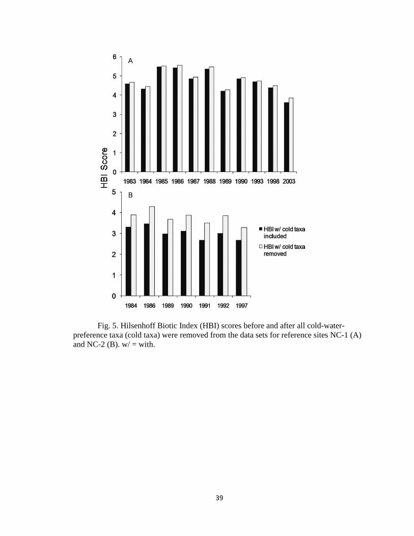
39

Fig. 5. Hilsenhoff Biotic Index (HBI) scores before and after all cold-water-preference taxa (cold taxa) were removed from the data sets for reference sites NC-1 (A)and NC-2 (B). w/ = with.

40

Fig. 6. Final site-condition classification scores before and after all cold-water-preference taxa (cold taxa) were removed from the data sets for reference sites NC-1 (A)and NC-2 (B). w/ = with, Mountain = Blue Ridge Mountain.

Blue Ridge Mountain-ecoregion scoring criteria were applied to Piedmont-

ecoregion reference sites (equivalent to replacing the Mountain ecoregion taxa with the

Piedmont ecoregion taxa) as an approximation of the outcome of range shifts of sensitive

taxa. In the most extreme case (i.e., complete community replacement), site-condition

classification of 1 Blue Ridge Mountain site decreased 1 level (from 5 to 4; Fig. 7A, B).

41

Fig. 7. Final site-condition classifications at 2 reference sites, NC0075 (A) andNC0248 (B), in the Piedmont ecoregion of North Carolina when Piedmont and BlueRidge Mountain (Mountain) scoring criteria were applied to the site data sets.

Modified metrics using temperature-preference traits

At site ME-1, the cold-to-total and warm-to-total ratios did not differ significantly

among coldest, hottest, and normal-temperature years for reference-site (Table 3). The

cold-to-total ratio appeared to be slightly higher during the hottest years. However, the

number of cold-water-preference taxa at this site was low, and the cold-to-total ratio was

so low that any apparent trend is misleading. The number of cold-water-preference EPT

42

taxa at this site, was too low to permit calculation of the cold-to-total EPT ratio.

At site UT-1, the cold-to-total ratio was significantly lower for the hottest-year

group than for the other year groups, but the warm-to-total ratio did not differ among year

groups (Table 3). The cold-to-total EPT ratio was lower and the warm-to-total EPT ratio

was higher for the hottest-year group than for other year groups, but the number of cold-

and warm-water-preference EPT was low, so these trends were not statistically

significant. At UT-2, the cold-to-total and cold-to-total EPT ratios were significantly

lower and warm-to-total and warm-to-total EPT was significantly higher for the hottest-

year group than for the other year groups (Table 3).

At site NC-1, none of the modified metrics differed among year groups (Table 3).

To visualize how much of the variation in the traditional EPT richness metric

could be explained by the temperature-preference modified metrics, we plotted all 3

metrics (EPT taxa richness, cold-to-total EPT, and warm-to-total EPT) by year for UT-1

and UT-2 (Fig. 8A, B). At site UT-1, EPT richness declined significantly over time (Fig.

8A). The warm-to-total EPT ratio did not change significantly over time. However, the

cold-to-total EPT ratio also decreased significantly over time, and the regression slope

was similar to the slope for total EPT richness. At site UT-2, total EPT richness and cold-

to-total EPT declined significantly over time, but the slope of the regression for cold-to-

total EPT was steeper (Fig. 8B). Moreover, the warm-to-total EPT ratio increased over

time (Fig. 8B).

43

Fig. 8. Linear regressions for Ephemeroptera, Plecoptera, Trichoptera (EPT)taxon richness and the ratio of cold- or warmwater- preference EPT taxon richness tototal EPT taxon richness vs year for reference sites UT-1 in the Uinta and WasatchMountains ecoregion (A) and UT-2 in the Colorado Plateau ecoregion (B) in Utah overthe period 1985 to 2005.

Discussion

Interactive effects of ecoregional characteristics and climate change on bioassessment

metrics

Evidence of invertebrate and other aquatic community responses to climate

change is accumulating, but the magnitude of effects from climate change is often low

compared the magnitude of effects of other large-scale spatial (e.g., land use) and

temporal (e.g., the North American Oscillation [NAO]) influences (Bradley and Ormerod

44

2001, Collier 2008, Chessman 2009, Sandin 2009). We found temperature-related

responses of benthic indicators and metrics that are consistent with long-term climate-

change effects and that could be used to establish future expectations for responses and to

understand implications of these responses to bioassessment-based decisions. Responses

were variable among sites and ecoregions, but they included decreases in richness or

relative abundance of cold-water-preference taxa, and in some areas, increases in warm-

water-preference taxa with increasing temperatures. These results are consistent with

those of other studies that have reported significant increasing or decreasing trends in

macroinvertebrates based on the thermophilic characteristics of the taxonomic group

(Daufresne et al. 2003, Durance and Ormerod 2007, Chessman 2009). Other widespread

responses among commonly used, taxonomically based metrics were declining richness

with temperature or over time of Ephemeroptera, Plecoptera, EPT, and total taxa. These

responses can alter reference communities to a degree that would affect decisions about

site condition. Site condition could be deemed degraded or even improved simply

because of taxon-specific responses to climate change.

Temperature-preference groups generally were sensitive to changing temperature

conditions, but responsiveness varied among ecoregions. Regional variations in projected

climate-change effects indicate that not all ecoregions are equally vulnerable to climate

change (USEPA 2007, NCAR 2008, Schoof et al. 2010). Many factors can influence

susceptibility to changing water temperature or hydrologic regime from climate change.

These factors include elevation (Cereghino et al. 2003, Diaz et al. 2008, Chessman 2009),

stream order (Minshall et al. 1985, Cereghino et al. 2003), degree of groundwater

influence, or factors that affect water depth and flow rate, such as water withdrawals

45

(Poff 1997, Poff et al. 2006a, Chessman 2009).

Many taxonomic metrics are based on mixtures of cold- and warm-water-

preference taxa, and the degree of mixing is related, in part, to ecoregional

characteristics, notably elevation. In all 3 states evaluated, a greater proportion of cold-

water-preference taxa occurred in higher-elevation ecoregions and a greater proportion of

warm-water-preference taxa occurred in low-elevation ecoregions (Table 2). Our results

suggested that elevation is one factor that drives the temperature-trait composition of

regional benthic communities. In turn, the temperature-trait composition of a community

affects the vulnerability of metrics and MMIs. State or tribal bioassessment managers

should consider focusing efforts to evaluate and modify MMIs first in the most

vulnerable, higher-elevation ecoregions.

Responses of commonly used metrics and MMI vulnerabilities

Utah.—Fairly predictable losses in EPT taxa richness (especially cold-water-

preference taxa) with increasing temperatures have occurred at high- and intermediate-

elevation sites in Utah. Projected EPT losses are as high as 40% by 2050. The potential

effect of this loss on bioassessment capabilities is too high to ignore. Moreover, this

projection of future losses was based on a linear estimate over time, but we have no

reason to assume that the actual rate of taxon losses will be linear, especially given year-

to-year and decadal-scale climatic variations. Thus, a linear estimate might be a poor

predictor of when southwestern regional MMIs or predictive models might become

incapable of differentiating reference from impaired sites.

Maine.—The Maine bioassessment protocol is based on a series of discriminant

46

models that require inputs of ~30 bioindicators. Therefore, other components of the

process of making decisions regarding site condition are vulnerable to climate change.

For example, Maine uses a group of Class-A indicator taxa as one metric for separating

Class-A from Class-B condition ratings. Class-A indicator taxa are evenly divided

between cold- and warm-water-preference taxa. As temperature increases, application of

this metric could confound results of the models because some of the Class A indicators

could decrease with increasing temperatures, whereas others could increase (USEPA

2010). In contrast, North Carolina uses only the HBI and EPT richness to classify site

condition. Both of these are vulnerable to effects of climate change on temperature-

sensitive taxa, but their effects on the MMI are direct and easy to understand. Thus, size

of the effect ultimately realized in MMI-based site-condition classifications will, in some

part, be modified by the complexity of the MMI used.

North Carolina.—The HBI is vulnerable to expected increases in water

temperature because changes in the temperature-trait composition of the community will

be confounded by the relationship between temperature preferences and pollution

tolerance. Decreases in cold-water-preference taxa with low HBI tolerance values or

increases warm-water-preference taxa with higher tolerance values will cause an increase

in the HBI. Because higher HBI values impart a more-impaired site-condition

classification, an increase in HBI driven by shifts in temperature-trait composition would

result in a concomitant decrease in site-condition classification. This vulnerability will be

stronger in regions like North Carolina where the correlation between pollution tolerance

and temperature preferences of taxa was strong and consistent. In other regions, such as

Maine, a more variable relationship, especially between warm-water-preference taxa and

47

HBI tolerances, could lead to variability in HBI vulnerability caused by spatial

differences in community composition of warm-water-preference taxa.

Modified metrics using temperature-preference traits

Cause cannot be determined from field observations or retrospective correlative

analyses. Moreover, causal assessment, like risk assessment, is retrospective rather than

prospective. However, causes must be considered to formulate corrective actions or to

make management or regulatory decisions. Therefore, interpretation of bioassessment

results often includes a process of inferring likely causes from environmental information

on the area being evaluated (e.g., chemistry, land use, watershed conditions, discharges),

species autecological information, and toxicological information (e.g., Beyers 1998, Suter

et al. 2002). The USEPA has structured this approach into a stressor-identification

process (USEPA 2000). In general, biological indicators, which are combined into MMIs,

are used for their diagnostic value (Verdonschot and Moog 2006). Sensitivity to climate

change and diagnostic capabilities of invertebrate indicators for this stressor have

received little consideration because climate change was not considered a stressor of

concern until recently. Thus, the effects of progressive changes in temperature and

hydrological regimes on existing metrics and MMIs are untested.

We focused on the relative contribution of cold- and warm-water-preference taxa

to particular component metrics with the intent of tracking of climate-related taxon losses

or replacements. Our preliminary evaluation indicates that a temperature-modified EPT

richness metric shows promise as a way to achieve this goal. Separate tracking of cold-to-

total EPT and warm-to-total EPT richness metrics successfully accounted for trends in

48

total EPT richness over time regardless of whether changes in total EPT richness were

caused by losses of cold-water-preference taxa (UT-1; Fig. 8A) or by losses of cold-

water-preference taxa plus gains of warm-water-preference taxa (taxon replacements;

UT-2, Fig. 8B).

Long-term increases in temperature have the potential to confuse the diagnosis of

altered conditions as defined by many bioassessment metrics. For example, decreases in

total richness or EPT richness, as observed at Utah reference sites, would be evaluated in

relation to a conventional stressor, such as organic pollution. However, we found that

decreases in cold-water-preference taxa and perhaps increases in warm-water-preference

taxa caused by increasing temperatures changed total and EPT richness metrics. The

magnitude of these changes was similar to the magnitude of changes caused by

conventional stressors that would lead to classification of a site as impaired. The

additional information provided by a temperature-modified metric could alter the way in

which site condition and probable causes are interpreted. In this example, the additional

information would support a shift from a presumption of pollution as the cause of the

reduction in the EPT richness metric to consideration of a temperature-related effect.

Without some attempt to modify traditional metrics to help characterize the contribution

of climate change to changes in metrics, erroneous conclusions might be drawn, and

conclusions of pollution effects or habitat degradation will be difficult to support.

We found a consistent moderate but significant relationship between temperature

sensitivity and sensitivity to organic pollution, defined in the context of the HBI. A

similar relationship was reported for the Ohio state biomonitoring data set (Rankin and

Yoder 2009, USEPA 2010). Thus, metrics selected because their component taxa are

49

generally sensitive or respond to conventional pollutants (Hilsenhoff 1987, Lenat and

Penrose 1996), also will be sensitive to climate-related changes in temperature and flow

conditions. Increasing organic pollution could alter the richness or relative abundances of

cold- or warm-water-preference taxa. Partitioning the HBI metric according to the

temperature-preference classification of component taxa could provide evidence to

distinguish probable effects of climate change from effects of conventional pollution.

This approach could be used in a weight-of-evidence context, supported by

documentation of both temperature trends and pollution status at a site.

Potential effects of losses of cold-water-preference taxa on MMI-based assessments

Estimated quantitative effects on site-condition classifications of changes in

community composition caused by changes in temperature-trait composition varied. In

some cases, changes in metric values were not sufficient to affect site-condition

classifications. In other cases, they changed by 1 level (e.g., from excellent to good, good

to fair). For example, in North Carolina, simulated loss of all cold-water-preference EPT

taxa because of increasing temperatures or community replacement (mimicking

migration of a warmer-water Piedmont community into the Blue Ridge Mountain

ecoregion) reduced site-condition classifications by 1 level. Full realization of either of

these 2 scenarios is unlikely and certainly would not occur in the near term. However,

they represent an upper bound on expected vulnerability of MMIs in the near future and

illustrate the immediate importance of testing and adopting temperature-modified metrics

into bioassessment analysis frameworks.

We evaluated preliminarily the ability of a modified metric to track temperature-

50

related species replacements, but we have not fully explored its ability to quantify the

proportion of changes caused by climate change from the proportion caused by other

stressors. Such an analysis would require investigation of modified metrics at a wide

variety of nonreference and reference sites, i.e., along a gradient of stressed conditions, to

examine combined responses to other stressors and to climate change. Proportional

changes in temperature-trait groups (using modified metrics) could be compared between

nonreference (conventional stressors plus climate change) and reference (climate change

only) sites to differentiate contributing causes.

The most valuable approach for incorporating modified metrics into an analytical

approach might be to continue calculating the traditional metric (e.g., EPT richness,

HBI), while adding new cold- and warm-water-preference metrics. In this way,

proportional changes in cold- and warm-water-preference taxa could be used to assess

how much of the difference in the total metric can be accounted for by changes in

temperature-trait groups. This comparison could be made over time or among locations

or groups of sites (e.g., reference and nonreference). This traits-based approach for

detecting and tracking effects of climate change is promising (Poff et al. 2010, Stamp et

al. 2010), given that few taxa (genera or species) in our study showed consistent climate-

related trends across the multiple sites and states analyzed.

We tested only a temperature-modified EPT richness metric, but other climate-

vulnerable and influential metrics (such as the HBI), metrics related to Ephemeroptera,

Plecoptera, or Trichoptera taxa, and community diversity metrics also should be modified

into new metrics that account for temperature preferences and tested within the

bioassessment framework. For example, a climate-tolerant metric could be used to help

51

separate responses to climate change and conventional stressors. Odonata, Coleoptera,

and Hemiptera (OCH) taxa have been used as a high-temperature/low-flow tolerant

indicator because of their prevalence in summer conditions, higher temperatures, and

lower flows (Bonada et al. 2007b). OCH taxa increased over time, with increasing

temperatures, or with lower precipitation at some sites in a study related to ours (USEPA

2010), results that support potential use of OCH as a climate-tolerant metric.

Limitations

Lack of information on temperature preferences for many taxa currently limits

development of climate-sensitive or climate-tolerant metrics. We used biomonitoring data

to develop temperature-preference and tolerance information for many taxa common to

Maine, Utah, and North Carolina (Stamp et al. 2010). Our approach could be used more

broadly to support development of temperature-modified metrics in other states.

Data limitations prevent differentiation among interannual, cyclical, and long-

term, directional climate changes. However, the larger issue might be how to use

biomonitoring data to distinguish effects of climate change from effects of other natural

and anthropogenic stressors. Durance and Ormerod (2008) discounted climate as the

cause of changes in stream benthic assemblages that were correlated with long-term (18

y) temperature increases at sites in southern England. They argued that some of the

faunal changes included taxa with traits (e.g., preferences for high flows and high

dissolved O2) that were contrary to expected responses to climate-driven increases in

stream temperatures. However, the observed biological responses used to project

biological-indicator and MMI vulnerabilities in our study were based on temperature

52

traits that are mechanistically linked to expected increases in water temperature

consequent to climate change. Our expectation of increasing temperature was

corroborated by significant (p < 0.05) long-term increasing trends in air or water

temperatures in several of the ecoregions evaluated and in numerous stream in the US

(Kaushal et al. 2010, USEPA 2010). Many observed metric and MMI responses were

consistent with temperature increases.

We used data from reference sites to minimize effects from conventional stressors

so that responses of benthic indicators to climatic variables could be evaluated

independently. However, several of our study sites potentially were affected by human

land uses (agricultural and urban). Landuse changes in the watersheds of reference sites

could have affect our long-term ability to separate climate change from other landscape-

scale stressors. Intensity of development-related land use at some of our long-term

reference sites has been relatively stable over the period of record (USEPA 2010). Thus,

the influence of urban and agricultural land use at those sites probably has been

consistent over the period of record. Nevertheless, the interactions of climate change and

development pose a substantial concern for biomonitoring programs in terms of data

interpretation and protection of sites in reference condition.

Few state biomonitoring programs have adopted landuse criteria for defining and

selecting references sites, and no widely accepted criteria exist. However, some

southeastern states (e.g., Georgia, Alabama, and South Carolina) apply landuse criteria

for selection of reference sites. These criteria are <15% urban plus <20% agricultural for

high-gradient streams, and <15% urban plus <30% agricultural for low-gradient streams

(Barbour and Gerritsen 2006). A broad spatial analysis of the relationships among

53

population density, land uses, water-chemistry constituents, and benthic community

characteristics in New England states led Snook et al. (2007) to associate best-available

reference conditions with ≤5% urban and ≤10% agricultural land use, a result that

supports an lower threshold for defining reference sites. Several of the reference sites

used in our study (2 in Maine and 1 in North Carolina) had >15% urban land uses, and

only a few reference sites available for our study, mostly in Utah, met the more stringent

criteria. Additional study and objective documentation to support specific landuse criteria

for definition of reference condition will be important for developing and adapting

biomonitoring programs to incorporate climate-change detection.

The period of record of a data set might determine our ability to use it to assess

effects of climate change. For example, in the Wasatch and Uinta Mountains and

Colorado Plateau ecoregions in Utah, detection of significant trends appeared to be

determined by the period of record of the data sets (trends detected at >14 y but not at

≤12 y). In the higher-elevation Northeast Highlands ecoregion in Maine, a period of

record of 11 y was apparently too short to define significant trends despite a

predominance of cold-water-preference taxa (USEPA 2010).

We rarely had >1 or 2 reference sites within an ecoregion with sufficient data to

conduct long-term trends analyses, even within the relatively extensive biomonitoring

data sets used in our study. For example, 105 reference sites were in the North Carolina

biomonitoring data set, but long-term data was available at only 3 of them. One site was

in the Blue Ridge Mountain ecoregion (11 y; Table 1), and 2 others had only 5 to 9 y of

data (USEPA 2010). Regional consistency of observed responses is difficult to determine

when spatial coverage and temporal replication are limited. We will need to understand

54

how many sites and how long a period of record are needed to detect effects of climate

change before we can modify and adapt biomonitoring programs to account for climate

change.

Acknowledgements

We thank the US EPA Global Change Research Program (GCRP) for providing

funding for this project through contracts GS-10F-0268K, DO 1101, and DO 1107 to

Tetra Tech, Inc., and the GCRP staff in the National Center for Environmental

Assessment (NCEA), especially S. Julius, for their input and advice throughout the

development of this project. We also thank staff in the Office of Science and Technology

in the US EPA Office of Water for their input and assistance; staff in state offices who

contributed data, reviewed approaches, and assisted with the development of the traits

database; and representatives on the regional workgroups for their input and review

during critical phases of the project. The views expressed in this article are those of the

authors and they do not necessarily reflect the views or policies of the US EPA.

55

Literature Cited

Allan, J. D. 1995. Stream ecology—structure and function of running waters. Chapmanand Hall, London, UK.

Barbour, M. T., and J. Gerritsen. 2006. Key features of bioassessment development in theUnited States of America. Pages 351–366 in G. Ziglio, M. Siligardi, and G. Flaim(editors). Biological monitoring of rivers: applications and perspectives. JohnWiley and Sons, Chichester, UK.

Barbour, M. T., J. Gerritsen, B. D. Snyder, and J. B. Stribling. 1999. Rapid bioassessmentprotocols for use in streams and wadeable rivers: periphyton, benthicmacroinvertebrates and fish. 2nd edition. EPA 841-B-99-002. Office of Water, USEnvironmental Protection Agency, Washington, DC.

Barbour, M. T., J. B. Stribling, and J. R. Karr. 1995. The multimetric approach forestablishing biocriteria and measuring biological condition. Pages 63–76 in W.Davis and T. Simon (editors). Biological assessment and criteria: tools for waterresource planning and decisionmaking. Lewis Publishers, Ann Arbor, Michigan.

Bêche, L. A., and V. H. Resh. 2007. Biological traits of benthic macroinvertebrates inCalifornia mediterranean-climate streams: long-term annual variability and traitdiversity patterns. Fundamental and Applied Limnology – Archiv fürHydrobiologie 169:1–23.

Beyers, D. W. 1998. Causal inference in environmental impact studies. Journal of theNorth American Benthological Society 17:367–373.

Böhmer, J., C. Rawer-Jost, and A. Zenker. 2004. Multimetric assessment of dataprovided by water managers from Germany: assessment of several different typesof stressors with macrozoobenthos communities. Hydrobiologia 516:215–228.

Bonada, N., N. Prat, V. H. Resh, and B. Statzner. 2006. Developments in aquatic insectbiomonitoring: a comparative analysis of recent approaches. Annual ReviewsEntomology 51:495–523.

Bonada, N., S. Dolédec and B. Statzner. 2007a. Taxonomic and biological traitdifferences of stream macroinvertebrate communities between Mediterranean andtemperate regions: implications for future climatic scenarios. Global ChangeBiology 13:1658–1671.

Bonada, N., M. Rieradevall and N. Prat. 2007b. Macroinvertebrate community structureand biological traits related to flow permanence in a Mediterranean river network.Hydrobiologia 589:91–106.

Bradley, D. C., and S. J. Ormerod. 2001. Community persistence among streaminvertebrates tracks the North Atlantic Oscillation. Journal of Animal Ecology70:987–996.

Burgmer, T., H. Hillebrand, and M. Pfenninger. 2007. Effects of climate-driventemperature changes on the diversity of freshwater macroinvertebrates. Oecologia(Berlin) 151:93–103.

56

Caissie, D. 2006. The thermal regime of rivers: a review. Freshwater Biology 51:1389–1406.

Cereghino, R., Y.-S. Park, A. Compin, and S. Lek. 2003. Predicting the species richnessof aquatic insects in streams using a limited number of environmental variables.Journal of the North American Benthological Society 22:442–456.

Chessman, B. 2009. Climatic changes and 13-year trends in stream macroinvertebrateassemblages in New South Wales, Australia. Global Change Biology. doi:10.1111/j.1365-2486.2008.01840.x.

Collier, K. J. 2008. Temporal patterns in the stability, persistence and condition of streammacroinvertebrate communities: relationships with catchment land-use andregional climate. Freshwater Biology 53:603–616.

Cuffney, T. F., M. D. Bilger and A. M. Haigler. 2007. Ambiguous taxa: effects on thecharacterization and interpretation of invertebrate assemblages. Journal of theNorth American Benthological Society 26:286–307.

Daufresne, M., P. Bady, and J.-F. Fruget. 2007. Impacts of global changes and extremehydroclimatic events on macroinvertebrate community structures in the FrenchRhône River. Oecologia (Berlin) 151:544–559.

Daufresne, M., M. C. Roger, H. Capra, and N. Lamouroux. 2003. Long term changeswithin the invertebrate and fish communities of the upper Rhone River: effects ofclimate factors. Global Change Biology 10:124–140.

Davies, S. P., and L. Tsomides. 2002. Methods for biological sampling and analysis ofMaine’s rivers and streams. DEP LW0387-B2002. Prepared for the State ofMaine Department of Environmental Protection. Maine Department ofEnvironmental Protections, Augusta, Maine. (Available from:http://www.state.me.us/dep/blwq/ docmonitoring/finlmeth1.pdf)

DeShon, J. 1995. Development and application of the Invertebrate Community Index(ICI). Pages 217–243 in W. S. Davis and T. P. Simon (editors). Biologicalassessment and criteria: tools for water resource planning and decision making.CRC Press, Boca Raton, Florida.

Diaz, A. M., M. L. Suarez Alonso, and M. R. Vidal-Abarca Gutierrez. 2008. Biologicaltraits of stream macroinvertebrates from a semi-arid catchment: patterns alongcomplex environmental gradients. Freshwater Biology 53:1–21.

Dolédec S, J. Dessaix, and H. Tachet. 1996. Changes within the Upper Rhône Rivermacro-benthic communities after the completion of three hydroelectric schemes:anthropogenic effects or natural change? Archiv für Hydrobiologie 136:19–40.

Durance, I., and S. J. Ormerod. 2007. Climate change effects on upland streammacroinvertebrates over a 25-year period. Global Change Biology 13:942–957.

Durance, I., and S. J. Ormerod. 2008. Trends in water quality and discharge confoundlong-term warming effects on river macroinvertebrates. Freshwater Biology.doi:10.1111/j.1365-2427.2008.02112.x.

Hawkins, C. P., R. H. Norris, J. N. Hogue, and J. W. Feminella. 2000. Development and

57

evaluation of predictive models for measuring the biological integrity of streams.Ecological Applications 10:1456-1477.

Hawkins, C. P., J. R. Olson, and R. A. Hill. 2010. The reference condition: predictingbenchmarks for ecological and water-quality assessments. Journal of the NorthAmerican Benthological Society 29(1):312–343.

Hering, D., R. K. Johnson, and A. Buffagni. 2006a. Linking organism groups – majorresults and conclusions from the STAR project. Hydrobiologia 566:109–113.

Hering, D., R. K. Johnson, S. Kramm, S. Schmutz, K. Szoszkiewicz, and P. F. M.Verdonschot. 2006b. Assessment of European streams with diatoms,macrophytes, macroinvertebrates and fish: a comparative metric-based analysis oforganism response to stress. Freshwater Biology 51:1757–1785.

Hering, D., R. K. Johnson, S. Kramm, S. Schmutz, K. Szosziewicz, and P. F. M.Verdonschot. 2006c. Assessment of European streams with diatoms,macrophytes, macroinvertebrates and fish: a comparative metric-based analysis oforganism response to stress. Freshwater Biology 51:1757–1785.

Hilsenhoff, W. L. 1987. An improved biotic index of organic stream pollution. GreatLakes Entomologist 20:31–39.

Hurd, B., N. Leary, R. Jones, and J. Smith. 1999. Relative regional vulnerability of waterresources to climate change. Journal of the American Water ResourcesAssociation 35:1399–1409.

IPCC (Intergovernmental Panel on Climate Change). 2001. Climate change 2001:impacts, adaptation, and vulnerability. Contribution of Working Group II to theThird Assessment Report of the Intergovernmental Panel on Climate Change.Cambridge University Press, Cambridge, UK.

Johnson, R. K., D. Hering, M. T. Furse, and R. T. Clarke. 2006. Detection of ecologicalchange using multiple organism groups: metrics and uncertainty. Hydrobiologia566:115–137.

Karr, J. R. 1991. Biological integrity: a long-neglected aspect of water resourcemanagement. Ecological Applications 1:66–84.

Kaushal, S. S., G. E. Likens, N. A. Jaworski, M. L. Pace, A. M. Sides, D. Seekell, K. T.Belt, D. H. Secor, and R. L. Wingate. 2010. Rising stream and river temperaturesin the United States. Frontiers in Ecology and the Environment (in press).doi:10.1890/090037.

Lenat, D. R. 1993. Development of a Hilsenhoff-type biotic index for North Carolina,with tolerance values for southeastern stream macroinvertebrates. Journal of theNorth American Benthological Society 12:279–290.

Lenat, D. R. and D. P. Penrose. 1996. History of the EPT taxa richness metric. Bulletin ofthe North American Benthological Society 13:305–306.

Minshall, G. W., R. C. Petersen, and C. F. Nimz. 1985. Species richness in streams ofdifferent size from the same drainage basin. American Naturalist 125:16–38.

58

Mouthon, J., and M. Daufresne. 2006. Effects of the 2003 heatwave and climaticwarming on mollusc communities of the Saone: a large lowland river and of itstwo main tributaries (France). Global Change Biology 12:441–449.

NCAR (National Center for Atmospheric Research). 2008. Regional climate-changeprojections from multi-model ensembles. University Corporation for AtmosphericResearch, Boulder, Colorado. (Available from: http://rcpm.ucar.edu)

NCDENR (North Carolina Department of Environment and Natural Resources). 2006.Standard operation procedures for benthic macroinvertebrates biologicalassessment unit. Division of Water Quality Environmental Sciences Section,North Carolina Department of Environment and Natural Resources, Raleigh,North Carolina. (Available from: http://h2o.enr.state.nc.us/esb/BAUwww/benthossop.pdf)

Norris, R. H., and M. T. Barbour. 2009. Bioassessment of aquatic ecosystems. Pages 21–28 in G. E. Likens (editor). Encyclopedia of inland waters. Volume 3. Elsevier,Oxford, UK.

Poff, N. L. 1997. Landscape filters and species traits: towards mechanistic understandingand prediction in stream ecology. Journal of the North American BenthologicalSociety 16:391–409.

Poff, N. L., and J. V. Ward. 1990. Physical habitat template of lotic systems: recovery inthe context of historical pattern of spatiotemporal heterogeneity. EnvironmentalManagement 14:629–645.

Poff, N. L., B. P. Bledsoe, and C. O. Cuhaciyan. 2006a. Hydrologic variation with landuse across the contiguous United States: geomorphic and ecological consequencesfor stream ecosystems. Geomorphology 79:264–285.

Poff, N. L., J. D. Olden, N. K. M. Vieira, D. S. Finn, M. P. Simmons, and B. C.Kondratieff. 2006b. Functional trait niches of North American lotic insects: traits-based ecological applications in light of phylogenetic relationships. Journal of theNorth American Benthological Society 25:730–755.

Poff, N. L., M. I. Pyne, B. P. Bledsoe, C. C. Cuhaciyan, and D. M. Carlisle. 2010.Developing linkages between species traits and multi-scaled environmentalvariation in streams to assess ability to detect benthic community responses toclimate change. Journal of the North American Benthological Society 29:000–000.

Sandin, L. 2009. The relationship between land-use, hydromorphology and river biota atdifferent spatial and temporal scales: a synthesis of seven case studies.Fundamental and Applied Limnology – Archiv für Hydrobiologie 174:1–5.

Sandin, L., and R. K. Johnson. 2000. The statistical power of selected indicator metricsusing macroinvertebrates for assessing acidification and eutrophication of runningwaters. Hydrobiologia 422/423:233–243.

Schoof, J. T., S. C. Pryor, and J. Surprenant. 2010. Development of daily precipitationprojections for the United States based on probabilistic downscaling. Journal ofGeophysical Research 115:D13106. doi:10.1029/2009JD013030

59

Snook, H., S. P. Davies, J. Gerritsen, B. K. Jessup, R. Langdon, D. Neils, E. Pizutto.2007. The New England wadeable stream survey (NEWS): development ofcommon assessments in the framework of the biological condition gradient.Prepared for the USEPA Office of Science and Technology, and the Office ofWatersheds Oceans and Wetlands, US Environmental Protection Agency,Washington, DC.

Stamp, J. D., A. Hamilton, L. Zheng, and B. Bierwagen. 2010. Use of thermal preferencemetrics to examine state biomonitoring data for climate change effects. Journal ofthe North American Benthological Society 29:000–000.

Suter, G. W., S. B. Norton, and S. M. Cormier. 2002. A methodology for inferring thecauses of observed impairments in aquatic ecosystems. EnvironmentalToxicology and Chemistry 21:1101–1111.

Tetra Tech, Inc. 2008. Draft Predictive Bioassessment Models for New Mexico Streams.Prepared for New Mexico Environment Department, Santa Fe, NM by TetraTech, Inc. Owings Mills, MD.

USEPA (US Environmental Protection Agency). 2000. Stressor identification guidancedocument. EPA-822-B-00-025. Office of Water and Office of Research andDevelopment, Washington, DC.

USEPA (US Environmental Protection Agency). 2002. Summary of biologicalassessment programs and biocriteria development for states, tribes, territories, andinterstate commissions: streams and wadeable rivers. EPA-822-R-02-048. Officeof Environmental Information and Office of Water, US Environmental ProtectionAgency, Washington, DC.

USEPA (US Environmental Protection Agency). 2007. Climate change effects on streamand river biological indicators: a preliminary analysis. EPA/600/R-07/085. GlobalChange Research Program, National Center for Environmental Assessment,Office of Research and Development, Washington, DC.

USEPA (US Environmental Protection Agency). 2010. Implications of climate changefor bioassessment programs and approaches to account for effects (ExternalReview Draft). Report No. EPA/600/R-10/085A. Global Change ResearchProgram, National Center for Environmental Assessment, Office of Research andDevelopment, US Environmental Protection Agency, Washington, DC.

UTDWQ (Utah Division of Water Quality). 2006. Monitoring manual. Utah Division ofWater Quality, Salt Lake City, Utah. (Available from:http://www.waterquality.utah.gov/Monitoring/06_DWQ_monitoring_manual.pdf)

Verdonschot, P. F. M., and O. Moog. 2006. Tools for assessing European streams withmacroinvertebrates: major results and conclusions from the STAR project.Hydrobiologia 566:299–309.

Vieira, N. K. M., N. L. Poff, D. M. Carlisle, S. R. Moulton, M. K. Koski, and B. C.Kondratieff. 2006. A database of lotic invertebrate traits for North America: U.S.Geological Survey Data Series 187. US Geological Survey, Washington, DC.(Available from: http://pubs.water.usgs.gov/ds187)

60

Wright, J. F., D. Moss, P. D. Armitage, and M. T. Furse. 1984. A preliminaryclassification of running-water sites in Great Britain based on macroinvertebratespecies and the prediction of community type using environmental data.Freshwater. Biol. 14:221-256.

Wright, J. F. 2000. An introduction to RIVPACS. Pages 1–24 in J. F. Wright, D. W.Sutcliffe, and M. T. Furse (editors). Assessing the biological quality offreshwaters: RIVPACS and other techniques. Freshwater Biological Association,Ambleside, UK.

Yoder, C. O., and E. T. Rankin. 1998. The role of biological indicators in a state waterquality management process. Environmental Monitoring and Assessment 51:61–88.

61

Appendix. Number of cold- and warm-water-preference taxa in each order in each statebioassessment data set. CWP = cold-water preference, WWP = warm-water-preference.

Order

Maine North Carolina Utah

CWP WWP CWP WWP CWP WWP

Arhynchobdellida 1 1

Basommatophora 4 1

Coleoptera 1 1 1 2 1 3

Decapoda 1 1

Diptera 7 10 10 5 8 2

Dorylaimida 1

Ephemeroptera 4 9 6 1 6 2

Haplotaxida 1

Hemiptera 1 1

Hoplonemertea 1

Hydroida 1

Isopoda 1 1

Megaloptera 1 7

Mesogastropoda 1

Odonata 2 1 1 1

Plecoptera 14 3 8 10 1

Rhynchobdellida 2

Trichoptera 10 6 6 4 7 5

Unionoida 1

62

CHAPTER 3

Implications of global change for the maintenance of water quality and ecologicalintegrity in the context of current water laws and environmental policies

Anna T. Hamilton1, Michael T. Barbour1, and Britta G. Bierwagen2

1Center for Ecological Sciences, Tetra Tech, Inc.

2Global Change Research Program, National Center for Environmental Assessment,

Office of Research and Development, U.S. Environmental Protection Agency

Anna.Hamilton@tetratech.com

Michael.Barbour@tetratech.com

Bierwagen.Britta@epa.gov

Abstract

There is both a fundamental and applied need to define expectations of changes in aquatic

ecosystems due to global changes. It is clear that programs using biological indicators

and reference-based comparisons as the foundation for assessments are likely to make

increasingly erroneous decisions if the impacts of global change are ignored. Global

changes influence all aspects of water resource management decisions based on

comparisons to reference conditions with impacts making it increasingly problematic to

63

find an “undisturbed” water body to define acceptable conditions of ecological integrity.

Using a more objective scale for characterizing reference conditions that is anchored in

expectations for what would be attainable under undisturbed conditions, such as the

Biological Condition Gradient (BCG) is one approach that maintains consistent

definitions for ecosystem conditions. In addition, protection of reference stations and of

unique or undisturbed aquatic resources is imperative, though the scope of protection

options is limited. Projections indicate that encroaching land use will affect 36-48% of

current reference surface waters by the year 2100. The interpretation of biological

indicators is also at risk from global changes. Distinguishing taxonomic attributes based

on temperature or hydrologic preferences can be used to enhance the ability to make

inferences about global change effects compared to other stressors. Difficulties arise in

categorizing unique indicators of global changes, because of similarities in some of the

temperature and hydrologic effects resulting from climate change, land use changes, and

water removal. In the quest for biological indicators that might be uniquely sensitive to

one global stressor as an aid in recognizing probable causes of ecosystem damage, the

potential similarities in indicator responses among global and landscape-scale changes

needs to be recognized as a limiting factor. Many aspects of global changes are not

tractable at the local to regional scales at which water quality regulations are typically

managed. Our ability to implement water policies through bioassessment will require a

shift in the scale of assessment, planning, and adaptations in order to fulfill our ultimate

regulatory goals of preserving good water quality and ecological integrity. Providing

clear expectations of effects due to global change for key species and communities in

64

freshwater ecosystems will help water quality programs achieve their goals under

changing environmental conditions.

Key words: Global change, climate change, water law, environmental policy,

bioassessment

The Underpinnings of Environmental Protection of Aquatic Resources

The expression of water laws and environmental policies is to protect the health of

aquatic ecosystems. The maintenance of natural ecological processes and ecosystem

function is paramount to addressing this goal. This is reflected in the U.S. Clean Water

Act (CWA, 1972) long-term goal of maintaining and restoring the ecological integrity of

aquatic systems, defined as comprising physical, chemical and biological integrity (CWA

1972). Similarly, the goal of the European Union Water Framework Directive (WFD),

Directive 2000), is to achieve “good status” of aquatic systems, including both “good

ecological status” and “good chemical status” (see Noges et al. 2009).

In principle, assessment of status is based on a combination of biological, physical,

and chemical indicators; however there is recognition that biological indicators are an

integrating response to all environmental conditions (Barbour et al. 2000, Moog &

Chovanec 2000). Based on this, in the U.S., biological assessment plays a central role in

numerous water quality programs that are components of the CWA. Bioassessment data

is used to assess water quality, identify biologically impaired waters, and develop

National Water Quality Inventory reports. It is used to develop biocriteria and set aquatic

65

life use categories, which represent different protection standards. Bioassessment data

are used to determine whether conditions of the waterbody support designated uses, and

if not, to develop total maximum daily load (TMDL) limitations for the pollutant(s)

contributing to the impairment. Bioassessment results are used to help identify causes of

observed impairments, based on the assumption that various components of aquatic

communities will respond differently to different types of stressors. Bioassessment is

used to determine the impacts of point source discharges as well as of episodic spills,

defining the extent of damage, responses to remediations, and supporting enforcement

actions. Other CWA programs that depend on bioassessment data include permit

evaluation and issuance, tracking responses to restoration actions, and other components

of watershed management. In Europe, the WFD emphasizes biological assessment

methods supported by the evaluation of hydromorphological and chemical parameters,

definition of strategies against pollution (combined approach for point and diffuse

sources), and establishment of river basin management plans (Chovanec et al. 2000).

Assessing the ecological health of rivers and streams is a fundamental and

increasingly important water management issue worldwide (Norris and Barbour 2009,

Bunn and Davies 2000) and relates directly to the preservation of ecosystem services of

aquatic resources. The concept of ecosystem services embraces those processes by which

the environment produces resources that we often take for granted, such as clean water,

and other services, such as mitigation of drought and floods, the cycling and transport of

nutrients, the maintenance of biodiversity, and detoxification and decomposition of waste

(Daily 1997, Postel & Carpenter 1997). Efforts such as the UN Millennium Ecosystem

66

Assessment (MEA 2005) are raising public awareness that high quality aquatic resources

provide society with ecological benefits and should be valued.

On a global scale, different countries are at varying levels of success in the endeavor

of protection and restoration of their water resources (Jungwirth et al. 2000). Those that

have had programs in place for many years have accomplished much in determining the

status of their resources and what must be done to restore degrading waters (Barbour &

Paul, 2010). However, few have considered how to effectively account for large-scale,

global changes, such as progressive climate change, increasing encroachment of

developed and agricultural land uses, and increasing human demands for freshwater, all

with ramifications to aquatic resources.

Water laws have historically focused more on point-source impacts than on landscape

or larger scales of pollution or habitat degradation. During the 20th century, the focus of

environmental problems has changed from local or regional issues like sewage discharge

in the first decennia towards global issues like climate change today (Verdonschot 2000).

This means that now, water resource management requires consideration of stressors that

operate at very different scales, such as climate change, which operates on a global scale.

It will alter air and water temperatures; alter flow and other hydrological parameters;

reduce ice and snow cover; alter the timing of snowmelt; alter stratification regimes in

lakes; increase sea levels; and increase salinity in some coastal areas (IPCC 2007).

Global changes in land use and water abstraction are landscape-scale stressors that are

directly related to human population increases.

67

An increase in the spatial scale of stressors implies a need to increase the spatial and

temporal scales of management and assessment (Verdonschot 2000). This change in

scale complicates the already complex management and restoration of impaired water

resources. While ecosystem management will be most effective when all stressors

impacting a resource are considered, certain aspects of global change impacts are not

tractable for control at a local, watershed, or state agency scale.

The environmental research community is engaged in understanding the effects of

global changes at a variety of spatial scales. Much of the research in the US on global

change and its effects on aquatic ecosystems are being supported by federal agencies,

such as the National Science Foundation (NSF), US Environmental Protection Agency

(U.S. EPA) and the National Oceanic and Atmospheric Administration (NOAA). The

European Union (EU) supports a series of research projects being conducted by several

institutions throughout Europe. The Australian government, through the Department of

Climate Change the Australian Greenhouse Office, and the Australian Climate Change

Science Program, also supports substantial research on climate change effects and

adaptations. As the effects of global changes become more evident and attention is

drawn to this complicating factor in maintaining good ecological status, scientists and

environmental managers should work together to ensure that the goals of environmental

protection are met. Research partnerships and information sharing may lead to more

effective resource management and decision-making tools that account for global change

effects.

68

Global Changes and Ecosystem Health

The concept of ecological health can be vague, but is generally borrowed from the

human health/medical paradigm, such that a “healthy” ecosystem, i.e., one with

“integrity”, is conceptually one that is functioning within “normal” ranges. We assume

this is true for pristine systems, but emphasize the question of whether an acceptable

level of ecological integrity exists in systems with some degradation, often termed

“minimally disturbed” or “leased disturbed” (Bailey et al. 2004, Stoddard et al. 2006).

Conditions observed in “minimally” or “least” disturbed streams or rivers often become

the basis for defining restoration or remediation goals, or for determining impairment, in

similar systems that are impacted by human uses and development.

The effects of land use alterations on river ecosystem condition have been reasonably

well studied (see for instance Paul & Meyer 2001, Allan 2004, Helms et al. 2009).

However, taking a global view of the future impacts of progressive land use changes on

ecosystem integrity is a more recent concern. There have been many studies of a variety

of water use and hydrological alteration impacts on stream ecological condition,

including flow regulation (e.g., Nilsson et al. 2005), increasing human uses (e.g., Bunn &

Arthington 2002), and hydrologic alteration in general (e.g., Richter et al. 2003, Konrad

et al. 2008). Now there is recognition that global changes in climate combined with a

growing world population and changes in global patterns of land use, socio-economics,

and technical changes in water resource utilization and management will combine to

increase water stress (i.e., decrease water availability and increase demand, Bates et al.

2008). Increased water stress will be particularly notable in regions where river runoff is

projected to decrease in the future, as well as in regions where water resources are

69

dependent on snow pack (e.g., the western U.S., the Mediterranean Basin (including

southern Europe, Northern Africa, and southwestern Asia), southeastern Australia,

southern Africa, and the west coast of South America) (Bates et al. 2008). Progressive

increases in regional water stress will put increasing demands on freshwater in likely

competition with ecological uses. This will bring conflicts in water use to a head, and put

greater pressure on management to consider all sources of impacts to water resources

(Brekke 2009).

Increasing attention has been given to whether ecosystem responses to climate change

are sufficient to cause concern and whether that concern should extend to our ability to

preserve and restore ecological integrity. Freshwater ecosystems are considered sensitive

to climate change impacts, owing to their fundamental dependence on hydrology and

thermal regimes, their dominance by poikilotherms, and the risks of interactions with

other stressors (Durance & Ormerod 2007). However, documentation of aquatic

biological responses to climate change on a basis that is meaningful to water quality and

resource managers has been slow in coming, with much early attention focused on

terrestrial ecosystems (e.g., Root et al. 2003, Thuiller 2004, Walther et al. 2002, 2005;

Parmesan 2006, Tobin et al. 2008, Suding et al. 2008, Zuckerberg et al. 2009). Climate

change effects in aquatic systems will manifest at all ecological levels (Fig. 1). Examples

of shifts in aquatic community structure that are relevant in a bioassessment framework,

documented in 10 relevant references, are presented in Table 1. Many of these effects

will be species and region specific; therefore, there is substantial variation in aquatic

biological responses that may impact the evaluation of ecological status. There will be

70

potentially major consequences both for ecosystem function and for the interpretation of

biomonitoring results relative to assessment of ecosystem health.

Fig. 1. Illustration of climate change effects on aquatic ecosystems and thesubsequent individual-, population-, and community-level responses to these changes.Effective indicators are those that respond to the consequences of climate change.

71

Table 1. Documented examples of shifts in aquatic community structure due to climatechange.

Examples of aquatic community changes Reference

increases in abundance, species richness, and proportion of southern and ofwarm-water species of fish in large rivers

Daufresne & Boet(2007)

loss of cold-water fishes from headwater streams, but also extension of moretolerant, thermophilic fishes from larger streams and rivers into newly suitablehabitat

Buisson et al. 2008

increases in fish species richness with increasing temperatures at higherlatitudes

Hiddink & Hofstede(2008)

displacement of upstream, cold-water invertebrate taxa with downsteam,warm-water taxa

Daufresne et al. (2004)

an increase in lentic and thermophilic invertebrates with increasingtemperature

Doledec et al. (1996)

reductions of spring abundance of dominant taxa, shifts in invertebrateassemblage composition from cooler to warmer water taxa, and possible losses(local extinctions) of more scarce taxa with increasing temperatures

Durance & Ormerod(2007)

significant long-term trends related to the thermophily and rheophily of benthictaxa, with groups preferring cold waters and higher flows declining

Chessman (2009)

changes in stability and persistence Collier (2008)

changes in species composition in lakes Burgmer et al. (2007)

changes in structure and diversity of riverine mollusk communities withreduction in community resilience during hot years

Mouthon & Daufresne(2006)

There are some similar and confounding effects among global changes that have

ramifications to the implementation of water policy. For example, stream temperatures

can be increased by climate change, and also by land uses (e.g., urbanization,

deforestation) (Table 2). Base flows can be reduced by climate change, and also by water

abstraction. Though the scale of these effects can be different, their similarities can make

it difficult to separate climate change impacts from those of other landscape-scale

stressors within management-relevant time frames. Climate change effects are also

compounded by other large-scale climate drivers such as the North Atlantic Oscillation

(NAO) (Bradley & Ormerod 2001). The presence of development and water abstraction

or diversion infrastructure can be documented independently, e.g., by quantification of

watershed land cover or water withdrawal data, which can help define contributing

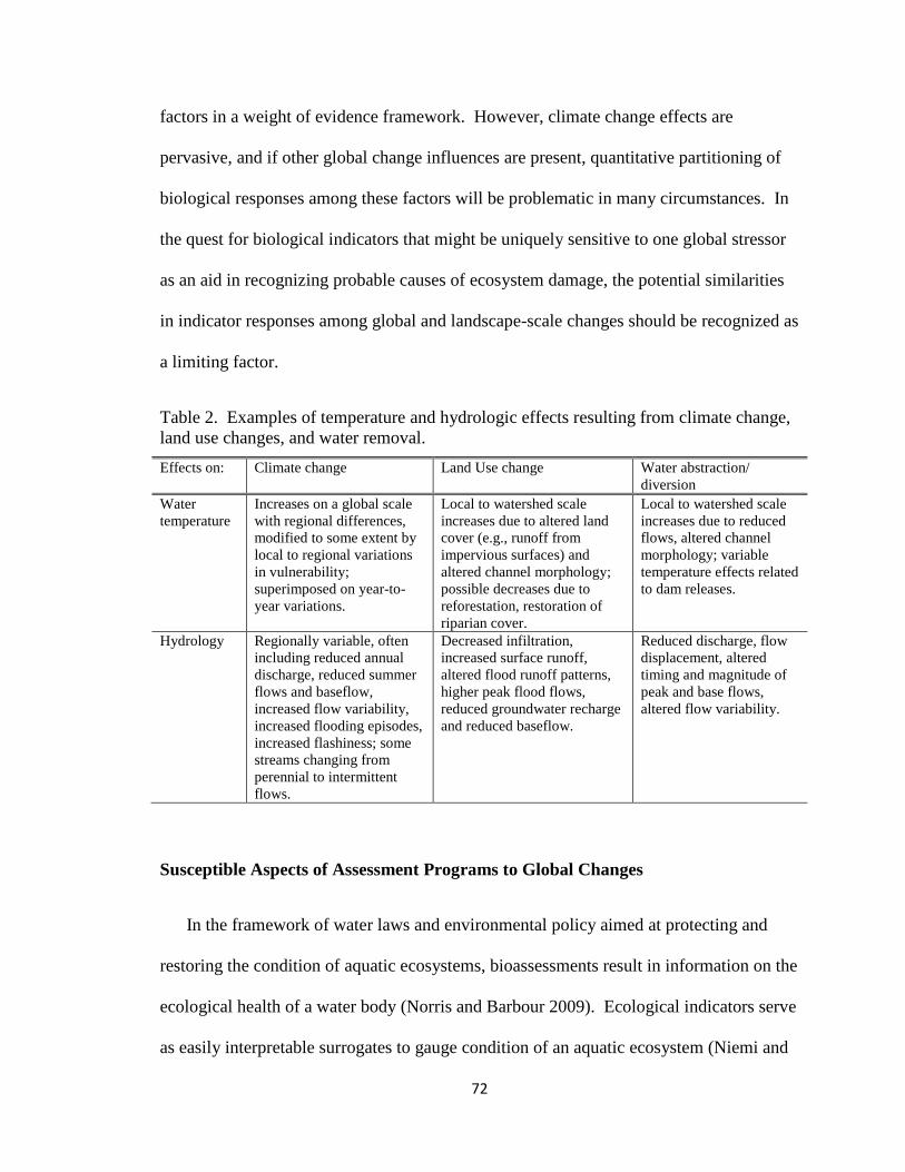
72

factors in a weight of evidence framework. However, climate change effects are

pervasive, and if other global change influences are present, quantitative partitioning of

biological responses among these factors will be problematic in many circumstances. In

the quest for biological indicators that might be uniquely sensitive to one global stressor

as an aid in recognizing probable causes of ecosystem damage, the potential similarities

in indicator responses among global and landscape-scale changes should be recognized as

a limiting factor.

Table 2. Examples of temperature and hydrologic effects resulting from climate change,land use changes, and water removal.

Effects on: Climate change Land Use change Water abstraction/diversion

Watertemperature

Increases on a global scalewith regional differences,modified to some extent bylocal to regional variationsin vulnerability;superimposed on year-to-year variations.

Local to watershed scaleincreases due to altered landcover (e.g., runoff fromimpervious surfaces) andaltered channel morphology;possible decreases due toreforestation, restoration ofriparian cover.

Local to watershed scaleincreases due to reducedflows, altered channelmorphology; variabletemperature effects relatedto dam releases.

Hydrology Regionally variable, oftenincluding reduced annualdischarge, reduced summerflows and baseflow,increased flow variability,increased flooding episodes,increased flashiness; somestreams changing fromperennial to intermittentflows.

Decreased infiltration,increased surface runoff,altered flood runoff patterns,higher peak flood flows,reduced groundwater rechargeand reduced baseflow.

Reduced discharge, flowdisplacement, alteredtiming and magnitude ofpeak and base flows,altered flow variability.

Susceptible Aspects of Assessment Programs to Global Changes

In the framework of water laws and environmental policy aimed at protecting and

restoring the condition of aquatic ecosystems, bioassessments result in information on the

ecological health of a water body (Norris and Barbour 2009). Ecological indicators serve

as easily interpretable surrogates to gauge condition of an aquatic ecosystem (Niemi and

73

McDonald 2004). They can also be early warnings of degradation that link appropriately

to the stressors expected in the system, which now include global changes in climate,

land use, and water use.

The effects of global change on bioassessment programs will vary regionally. Land

and water use effects are largely driven by locations of and projected future changes in

major population and agricultural centers. Differences in climate change threats and

responsiveness are instead driven by regional variability in climate, as well as regional

differences in the vulnerability of aquatic ecosystems. Differences in regional climate

and disturbance regimes are important contributors to species sensitivities to

environmental changes (Helmuth et al. 2006). Many factors can influence susceptibility

to changing water temperature or hydrologic regime due to climate change, such as

elevation (Cereghino et al. 2003, Diaz et al. 2008, Chessman 2009), stream order

(Minshall et al. 1985, Cereghino et al. 2003), degree of ground water influence, or factors

that affect water depth and flow rate, such as water withdrawals (Poff 1997, Poff et al.

2006a, Chessman 2009).

Essential components of the assessment and management of ecological health include

the reference condition paradigm and the use of biological indicators. In a regulatory

context, impairment represents a level of departure from defined reference conditions

considered unacceptable for maintenance of ecological integrity. However, the continued

good status of reference locations, and therefore their use as a basis for comparison, is

significantly threatened by global change. Both climate change effects and encroachment

of development can be expected to impact streams that were previously categorized as

minimally altered, probably more so than previously conceived or documented. We have

74

found that in some examples from state biomonitoring data in the U.S. losses of cold-

preference taxa and replacement by warm-preference taxa had the potential to degrade

the condition classification of reference stations by a full level (e.g., from “excellent” to

“good”, or “good” to “fair”), as defined by the particular state bioassessment schema

(Fig. 2) (USEPA 2010).

Fig. 2. Final bioclassification (station quality) scores at a North Carolina referencesite in the Blue Ridge Mountain ecoregion (NC0209) before and after all cold-preferencetaxa are eliminated from the observed benthic invertebrate community.

Land use impacts on reference stations have long been considered a factor that can be

controlled in the process of selecting sampling stations. However, finding undisturbed

reference conditions is already a challenge in the U.S. and Europe (e.g., Herlihy et al.

2008, Noges et al. 2009), and often the only comparisons for assessment are to the “best

of what is left”, or least disturbed conditions (Stoddard et al. 2006). For state

75

biomonitoring programs in the U.S., it is often the case that the extent of developed land

uses affecting established reference locations is not quantitatively documented, nor

updated over time. We have found that the influence of urban/suburban land uses on

established reference locations can be greater than previously assumed. In one example,

20-25% of reference sites classified as high quality in Florida were actually surrounded

by >20% urban/suburban land uses (Fig. 3). Furthermore, using spatially explicit

projections of population growth, it was estimated that by the year 2100, from 36% to

48% of current reference locations could be compromised by encroachment of developed

land uses (Fig. 3) (USEPA 2010).

Fig. 3. Percent of existing Florida reference stations (N=58, classified as“exceptional”), that have >20% developed land use (with 25 houses per square mile ormore) within a 1-km buffer surrounding the station; for current land use conditions, andfor projected developed land use distributions consistent with IPCC (2000) base case, A2and B1 scenarios, projected for decadal time periods through 2100 (from U.S.EPA 2010).

76

The combined effects of climate change and land use encroachment are thus reducing

availability of reference locations for comparative analyses, and definition of the

reference baseline will continue to shift toward more degraded conditions (“reference

station drift”, Fig. 4). Noges et al. (2007) suggest that in Europe, climate change will

alter reference conditions enough to potentially alter typologies (classifications) and

impact restoration targets. They point to the need for periodic re-evaluation and

adjustment of reference conditions and associated standards to accommodate climate

change effects that cannot be mitigated. With regard to the Clean Water Act (CWA), this

might be interpreted as a lowering of standards in conflict with anti-degradation policies.

Fig. 4. Hypothetical example of reference station drift over time as climate changedegrades the condition of sites, based on classification of stations along a BiologicalCondition Gradient (BCG).

The influence of global change thus poses a serious risk to management decisions

regarding environmental protection and restoration. Unaccounted climate change

77

impacts, especially when further compromised by increasing influence of developed or

agricultural land uses, are likely to lead to fewer determinations of impairment and

listings of impaired stream reaches. This is expected because biological responses to

climate change, such as decreases in mean abundances or species richness of cold-

preference or other sensitive taxa and trait groups, increases in warm-preference or other

tolerant taxa and groups (U.S.EPA 2010), and increases in the variability of these

indicators, drive reference sites to greater similarity with non-reference areas, as well as

greater difficulty in establishing statistical differentiation (USEPA, 2008). Overall,

progressive under-protection of water resources can be expected.

The interpretation of biological indicators and metrics is also at risk from global

changes. Several traditional, taxonomically-based biological metrics, including total

species richness; Ephemeroptera (mayflies)- Plecoptera (stoneflies)- Trichoptera

(caddisflies)- (EPT) abundance and richness metrics; and Hilsenhoff’s biotic index

(HBI), are shown to be composed of both cold- and warm-water preference taxa (U.S.

EPA 2010). The relative contribution from cold- and warm-preference taxa varies

regionally and among metrics (U.S.EPA 2010). This mixed composition of temperature

traits leads to differential responses to climate-associated increases in water temperature

over time, and therefore, the vulnerability of that metric to climate change effects. If a

metric like EPT richness is evaluated in a vulnerable location where cold-preference taxa

are declining over time, the EPT metric would decline with the potential to alter the

ecological status rating of that location. This could happen due to climate change in the

absence of any other impairment to the water resource conditions at that location. In

another example, we have found a widespread, moderate but significant relationship

78

between temperature sensitivity and sensitivity to organic pollution (U.S. EPA 2010).

Thus, metrics such as Hilsenhoff’s Biotic Index (HBI), originally adopted to represent

responses to organic pollution, are susceptible to changes in index values due only to

climate change effects. The magnitude of biological responses due to climate change-

mediated increases in temperature may be sufficient to cross thresholds of impairment

and alter management decisions (U.S. EPA 2010). Without accounting for these climate

responses, the traditional interpretation of changes in EPT, HBI, or other metrics could be

in error and increase the uncertainty of currently employed processes of impairment

characterization and interpretation of causes.

Tracking long-term responses in trait groups defined by temperature preferences is a

means to determine biological responses to global changes in temperature (Poff 1997).

Categorization by traits reduces variation across geographical areas that can be associated

with taxonomic composition, and thus supports analyses of regional or larger-scale data

sets. Such regional-scale analyses are consistent with the larger scale of global change

effects. Evaluation of temperature trait groups that are subsets of traditional

taxonomically-based metrics also illustrates the vulnerabilities of current bioassessment

metrics.

Predictive models such as the River Invertebrate Prediction and Assessment

Classification System (RIVPACS) used to assess condition and make compliance or

other regulatory decisions are susceptible to responses to climate change, predominantly

through the relative composition of cold- and warm-preference trait groups in the

“observed communities” (O in the O/E [observed/expected] index) (U.S. EPA 2010).

The predictive models for expected communities may be more robust to climate change

79

than individual indices, given periodic model recalibration, due to the relative stability of

using long-term averages in estimating predictor variables (U.S. EPA 2010). The process

of periodic recalibration may still have the undesirable effect of altering the reference

baseline of comparison over the long term.

Integration of Monitoring and Assessment for Global Change into Environmental

Policy

It is clear that programs using biological indicators and reference-based comparisons

as the foundation for assessments are likely to make increasingly erroneous decisions,

especially in the most climatically vulnerable or in increasingly populated regions and

watersheds, if the impacts of global change are ignored. Conversely, programs that adapt

their biological assessment framework by characterizing global change vulnerabilities

and sensitive ecological traits will be in a better position to make informed decisions

regarding the synergism of multiple stressors in the context of global changes. We have

highlighted several critical components of the typical water quality management process

that are demonstrably vulnerable to global change impacts. These include impacts to

biological indicators that dissociate their responses from conventionally interpreted

causes; degradation of reference conditions that will rapidly make it difficult or

impossible to define desirable levels of ecological integrity; and the synergism of global

changes that will alter water distribution and availability and increase the uncertainty

under which flows needed to maintain ecological functioning will be maintained. If

assessment approaches are not modified, the increasing loss of aquatic habitat to global

80

shifts in abundance and distribution of flowing waters will become institutionalized

because of lack of action to deal with the implications of global change. This will

introduce additional uncertainty into a system that requires knowledge of relatively

predictable biological indicator responses to different types of “conventional” stressors.

The framework for a new approach needs to address these major vulnerabilities in a

manner that accommodates the inherent scale differences between “global change”

stressors and many conventional stressors. We recognize that many aspects of on-the-

ground implementation of water policy and water quality management will continue to be

at a local (e.g., stream reach) level. Local actions that are augmented with a regional (or

larger) scale focus will allow bioassessment and implementation of water law and policy

to incorporate considerations of global change stressors. Any supplementary monitoring

or analyses at a regional scale should also provide inputs that are meaningful at the local

scale.

What do we do about loss of reference conditions? Global changes influence all

aspects of making water resource manage decisions that are based on comparisons to

reference conditions. Clearly it will become increasingly problematic to find an

“undisturbed” water body of a particular type as a way to define acceptable conditions of

ecological integrity. The baseline described from existing reference locations will

increasingly reflect only the best available or least disturbed among available locations,

and so will reflect increasingly degraded conditions. As stated earlier, the option of

periodic recalibration of reference conditions based on what is left leads directly to

acceptance of widespread and institutionalized degradation of water quality conditions

and calls into question how anti-degradation policies, typically included in water quality

81

regulations in the U.S., can be managed considering the additional influences of climate

change. There needs to be a basic understanding that recalibration of reference in a

downward direction should never be done. Use of a biological condition gradient

approach will aid in anchoring the reference condition founded on an achievable schema

(Davies and Jackson 2006). Special attention of management and regulatory agencies

will be needed to consider implementation of anti-degradation policies with respect to

global changes.

On the other hand, there will have to be consideration given in some circumstances

to the possibility that global changes may lead to irreversible changes in habitat

conditions over the long term that may irretrievably alter attainable ecological conditions

and uses. For example, some cold water streams could take on cool water characteristics,

with declining abundances or richness of sensitive cold water taxa and possible increases

in warm-water taxa. Regulated parameters such as temperature, dissolved oxygen, and

ammonia, may also be sensitive to climate change effects, and their values may need to

be adjusted relative to revised designated uses (Table 3). Refinement of aquatic life uses

can be applied to guard against lowering of water quality protective standards. More

refined aquatic uses could create more narrowly defined categories, which could

accommodate potentially “irreversible” changes, but with sufficient scope to maintain

protection and support anti-degradation from regulated causes. In addition, the

application of use attainability analyses (UAA) on vulnerable water bodies may be

pertinent for characterizing climate impacts.

82

Table 3. Variables addressed in criteria and pathways through which they maybe affected by climate change (from Hamilton et al. 2009).

Criteria Climate change impacts

Pathogens Increased heavy precipitation and warming water temperatures may require the evaluationof potential pathogen viability, growth, and migration.

Sediments Changing runoff patterns and more intense precipitation events will alter sedimenttransport by potentially increasing erosion and runoff.

Temperature Warming water temperatures from warming air temperatures may directly threaten thethermal tolerances of temperature-sensitive aquatic life and result in the emergence ofharmful algal blooms (HABs), invasion of exotic species, and habitat alteration.

Nutrients Warming temperatures may enhance the deleterious effects of nutrients by decreasingoxygen levels (hypoxia) through eutrophication, intensified stratification, and extendedgrowing seasons.

Chemical Some pollutants (e.g., ammonia) are made more toxic by higher temperatures.

Biological Climate changes such as temperature increases may impact species distribution andpopulation abundance, especially of sensitive and cold-water species in favor of warm-tolerant species including invasive species. This could have cascading effects throughoutthe ecosystem.

Flow Changing flow patterns from altered precipitation regimes is projected to increase erosion,sediment and nutrient loads, pathogen transport, and stress infrastructure. Depending onregion it is also projected to change flood patterns and/or drought and associated habitatdisturbance.

Salinity Sea level rise will inundate natural and manmade systems resulting in alteration and/orloss of coastal and estuarine wetland, decreased storm buffering capacity, greater shorelineerosion, and loss of habitat of high value aquatic resources such as coral reefs and barrierislands. Salt water intrusion may also affect groundwater.

pH Ocean pH levels have risen from increased atmospheric CO2, resulting in deleteriouseffects on calcium formation of marine organisms and dependent communities and mayalso reverse calcification of coral skeletons.

Detecting and monitoring shifting conditions in the reference population should be

part of any water quality program. As described earlier, a more objective scale for

defining ecological condition, and thus for characterizing reference conditions, that is

anchored in expectations for what would be attainable under undisturbed conditions will

be integral to such a program. While seemingly a tall order, developing a scale of

condition that reflects the full range of biological potential for a region would have two

values as an adaptation of the process of bioassessment in the face of global changes.

First, it would allow existing reference locations to be ranked in terms of ecological

status, where such ranking could be corroborated with documentation of existing levels

83

of land use encroachment, water withdrawals and flow alterations. Second, it would

define the scale against which future reference station degradation from combined global

change impacts could be tracked and quantified. Characterization of conditions at test

locations would utilize the same scale, and relative changes between reference and test

conditions would provide one piece of evidence in the evaluation of contributions of

global and conventional stressors to impairment.

An example of an objective scale of condition is the Biological Condition Gradient

(BCG), which has been under research and development by the U.S. EPA (Davies and

Jackson 2006). Its application in general is justified as supporting a more uniform

interpretation of condition. This approach would also establish a best estimate of

undisturbed biological potential, and therefore a reference a baseline against which to

track future global changes. This would be a valuable adaptation of the existing

bioassessment approach, and in the long term would help meet the objectives of

maintaining and restoring good levels of water quality and ecological integrity. It is

highly recommended that an objective scaling of biological condition, such as the BCG,

be given much greater focus and support at the national and regional scale.

Development of an objective scale for characterizing ecological status and condition

would have to be regional and be supported by classification of river system types

(development of typologies). This follows the need to define reference conditions

regionally within types, an approach used in the US (e.g., Gerritsen et al. 2000, Barbour

and Gerritsen 2006), Europe (e.g., Verdonschot 2006, Noges et al. 2007), and Australia

(e.g., Kennard et al. 2006). BCGs have been developed for some regions in the US (e.g.,

Gerritsen and Leppo 2005). However, there is still a legacy of conducting site-specific

84

condition assessments based on comparison to an “upstream” reference site or using a

paired-watershed approach. Site-specific comparisons cannot capture or account for

effects of large scale, pervasive global changes outside of a regional context that defines

the range of variation of conditions that exist for that water body type.

Implicit in tracking and accounting for global changes as a part of bioassessment is a

time component to sampling and analyses. Despite the relatively large number of

reference stations that may be sampled within a jurisdiction or ecoregion, there are

typically few stations that are sampled repeatedly and have long-term data. Preservation

of adequate long-term data records, with ongoing, regular (at least annual) monitoring is

desirable to increase the robustness of water program assessments to the confounding

effects of climate change. Adequate long-term monitoring can be a burden for local to

regional management agencies. Considering the desirability of repeated temporal

monitoring with the recommendation that reference conditions be established on a

regional basis, it is recommended that a network of comprehensive monitoring locations

be established and maintained. A regional level of implementation would be consistent

with the scale of controlling factors in climate change patterns and vulnerabilities, such as

climatic type, geology, topography, elevation, ground water influence, latitude,

vegetation, etc. Such conditions often cross state, tribal or other jurisdictional

boundaries. Collaboration would be best suited in a modest initial focus of monitoring

vulnerable areas and watershed types.

Environment agencies are charged with embracing the concept of protecting

remaining high quality stream reaches that define reference conditions, mostly at the

watershed management scale (e.g., Palmer et al. 2009). However, the range of possible

85

protective actions is limited, and for the most part, only addresses climate change

indirectly. Protection options encompass minimization, mitigation, and/or buffering from

land-use impacts of non-point source runoff, erosion, and hydrologic changes, as well as

consideration of water withdrawal impacts. Categories can include socio-political action

at the municipal to state scale, such as zoning restrictions, green building incentives,

riparian buffer zones, designation of conservation zones or protected areas (e.g.,

preserves, national parks or forests, wilderness areas), implementation of environmental

flow regulations, or other limitations on water withdrawals or diversions from particular

stream reaches. Protection actions can be valuable on a local to regional scale, and can

be targeted at high quality or unique aquatic resources (Palmer et al. 2009). However,

there are often disconnects between the agency with interest in protection of high quality

reference locations (e.g., state environment or natural resource departments) and the

agencies with the authority to implement such actions. In addition, implementation of

comprehensive protection measures takes time, which is in short supply relative to

impacts from global changes which are happening now. Given the existing and future

projected levels of global change impacts to aquatic resources, targeted protection cannot

be solely relied on to maintain the future viability of bioassessment and implementation

of water policy.

How do we Resolve Mixed Messages from Existing Biological Indicators?

Appropriate indicators for assessing ecological status and integrity depend on the

vulnerability of potential indicators to the range of stressors being tracked, their ease of

measurement and interpretability, and the applicability of the information they provide at

the spatial or temporal scale of interest. Indicators can be drawn from a wide range of

86

ecosystem properties, including functional and structural components, production and

metabolism, nutrient use and cycling, energy supply, and species composition and

feeding types represented in its biotic assemblages (Allan and Castillo 2007). There is

increasing emphasis on using measures that reflect functional processes (Paul 1997,

Fellows et al., 2006), or that incorporate both ecosystem structure and function (Udy et

al. 2006). Moss (2008) argues that true properties of ecological quality include efficiency

of nutrient use, habitat connectivity, mechanisms of resilience, and characteristic

biological structures and functions, but not necessarily a characteristic species list; and

that biomonitoring should not rely mainly on taxonomic indices. Still, it is widely

accepted and applied in bioassessment that characteristics of biological assemblages,

including both taxonomic and trait groups, strongly reflect ecosystem status and health

(Bonada et al. 2007a, b, Johnson and Hering 2009, Norris and Barbour 2009).

Difficulties arise in categorizing unique indicators of global changes, because of

similarities in some of the temperature and hydrologic effects resulting from climate

change, land use changes, and water removal (Table 2). In addition, climate change is a

global influence in the environment, which differentiates it from most conventional

stressors, including land use and water demand changes, which are landscape-scale

stressors with global implications. Biomonitoring tools should be tailored to the types

and scales of stressors expected. If it is a fundamentally sound concept that larger scale

(global change) stressors require a comparably large scale of assessment and

management, then both the selection of potential indicators and the way they are used in a

bioassessment framework must be appropriate for regional (or larger) scale application.

This will require a conscientious refocusing of water policy implementation from the

87

local scale fostered by the current stream reach-specific listing process, to a watershed

scale or larger scale, integrated approach to evaluation and management.

With increasing knowledge of the types of biological responses to climate change

evident around the US, Europe, and elsewhere, as well as the categories of organisms that

are showing relatively predictable responses, it may become possible to adjust

bioassessment metrics to enable a clearer interpretation of stressor identification and

causal analysis. In a management or regulatory context, biological indicators likely to

express the strongest, most regionally consistent and interpretable responses to climate

variables will be most effective to document effects early and establish credible links

between causes (i.e., the stressor of climate change) and observed biological responses.

Groupings of macroinvertebrates (or other organisms used in bioassessment) based

on ecological traits related to temperature or hydrologic preferences provide a link to

temperature- and flow-related global change effects. They are interpretable with regard

to causal relationships, though with limitations, and offer predictive ability and

transferability among regions (Lamouroux et al. 2004, Poff et al. 2006b, Horrigan &

Baird 2008, Verbeck et al. 2008a, 2008b). Trait-based analysis may increase the

diagnostic power of taxon-based bioindicators (Dolédec et al. 2000) and contribute to a

broader understanding of environmental stressor responses (Dolédec & Statzner 2008).

We have already indicated that complete separation of climate change and other global

changes will often be difficult and is unlikely to be accomplished through a single

biological indicator unique to a specific global stressor. Nevertheless, we propose that

separating taxonomic metrics (e.g., EPT taxa, HBI) into sub-categories based on

temperature preferences can be used to enhance the ability to make inferences about

88

global change effects compared to other stressors. Tracking metrics by temperature

preference would provide a mechanism for documenting climate change-related taxa

losses or replacements; this could be used in conjunction with other stressor data and

trends at reference locations to help differentiate among global and conventional stressor

contributions to observed responses.

Preliminary evaluations have been undertaken of the efficacy of separating

taxonomic metrics, such as metrics related to EPT taxa, and the HBI, into new metrics

that account for temperature preferences of the component taxa (e.g., a ‘cold-EPT

richness’ metric, etc) (U.S. EPA 2010). Additional testing of potential climate-revised

metrics would be needed on a regional basis.

Continued success in associating biological responses with probable causes of

impairment will require redefinition and recalibration of many traditional metrics. In

terms of policy implications, it is likely that such efforts would be viewed by local

resource managers as extensive. ‘Federal’ agencies are already providing support in the

form of substantial trait data bases (e.g., Schmidt-Kloiber et al. 2006, U.S.EPA 2010).

Additional regional efforts to define temperature traits will be needed to provide an

important component in the foundation for evaluating climate change affects on aquatic

ecosystems. If the relative contributions from the major global changes can not be

reliably separated, this weakens specific impairment or other management decisions with

the potential effect of losing the confidence of the regulated community.

Why Embrace A Management Paradigm Shift? The legacy of focusing on point

sources of pollution carries an additional legacy of justifying remedial action based on

89

cause. ‘Punishment of the guilty’ describes the assessment and management of point

sources of pollution, in which the imposition of some regulatory action (e.g., permit

limits, mitigations, restoration requirements) is justified based on specific attribution of

the cause of impairment. This approach gives a narrow focus to the process of water

resource quality protection and restoration and does not encompass adaption strategies to

address and manage global change impacts. We recognize there will always be local

pollution problems that require local solutions; thus, examination of local causes will

continue to be applicable in the context of defining impairment from point source

dischargers, supporting issuance and re-issuance of discharge permits, tracking responses

to specific restoration actions, and developing total maximum daily load (TMDL) limits.

However, local management for preservation of ecological integrity also is impacted by

stressors at non-local (global) scales; hence, the need to utilize multiple scales of

assessment.

Recognize the management implications of the discontinuities between the scale

of global stressors, the scale of the indicators employed in the assessment process (local

to regional), and the scale of management options (local to regional) is a first step in

developing an appropriate response. The causes of climate change cannot be altered at

the scale of most water resource management activities. Even if maximum reductions of

greenhouse gas emissions were achieved immediately on a national to global scale,

“committed” climate responses would continue for decades. Similarly, population

growth along with increases in developed and agricultural land uses will continue, as will

demands for human uses of fresh water, outside of the purview of local water quality

90

agencies. But water resource managers are still faced with protection or restoration of

good water quality and ecological integrity.

In the context of climate change it is increasingly important to consider adaptation

strategies or other management actions for remediation or restoration that are not

necessarily directly related to the proximal cause of the problem. This is a diverse

concept that has been touched on by the IPCC (“no regrets” adaptations, IPCC 2001) and

the U.S. Climate Change Science Programs (CCSP 2008). We suggest that managers be

encouraged to consider actions that can improve or ameliorate an impaired condition in

an aquatic system, considering broad factors such as feasibility of implementation,

possibility of multiple environmental benefits, and direct or indirect impacts on

conditions of concern. The actions may not be directly related to the causes of concern,

but given the increasing likelihood that multiple causes may be contributing to a

particular condition at multiple scales, this is inevitable. Adaptations can be selected to

have recognizable environmental benefits, whether projected global changes ultimately

impact the site or not (“no regrets” adaptations). The need to take whatever management

actions that may be feasible is starting to be recommended in response to climate change

in particular (Palmer et al. 2009).

In the US, the U.S. EPA develops the scientific basis for water law and environmental

policy actions and provides recommendations and guidance to state water quality

agencies for implementation. In Europe, the guiding principal is the Water Framework

Directive and the oversight organization that includes representatives of the partner

countries. Each country is then charged with the mandate to implement the Directive.

91

Regardless, the agency with the responsibility of assessing and protecting its water

resources should help advance a revised assessment process, including inputs on:

Methods and criteria for evaluating the relative vulnerabilities of regions or

watersheds to global change effects, focusing on alterations to thermal and

hydrologic regimes, and future projections of land use patterns. Assessments

should use objective criteria to define vulnerabilities. Providing clear

expectations of effects due to global change for key species and communities in

freshwater ecosystems will help these programs achieve their goals under

changing environmental conditions.

Support of additional research needs through agency and academic channels,

including focus on how to implement program modifications, BCG

implementation, traits and biotic response data base expansion, and metrics

modifications.

Development and implementation of more sophisticated watershed modeling to

bridge the scale gap between General Circulation Models (GCMs) and watershed

responses. The EuroLimpacs project of the EU has done much in this regard

(e.g., Whitehead et al. 1998a, 1998b, 2002; Wade et al. 2002). In the US, EPA’s

Global Change Research Program is supporting research to evaluate the impacts

of climate change and urbanization on hydrology and water quality in twenty

major river basins throughout the US.

92

Acknowledgments

The authors would like to thank L. Yuan, R. Novak, K. Metchis, and several anonymous

reviewers for their comments, which greatly improved this article. The Global Change

Research Program in the National Center for Environmental Assessment in the U.S.

Environmental Protection Agency’s Office of Research and Development provided

financial support for the analyses contributing to this article through contract # GS-10F-

0268K, DO 1107 to Tetra Tech, Inc. The views expressed in this article are those of the

authors and they do not necessarily reflect the views or policies of the U.S.

Environmental Protection Agency.

References

Allan, J.D. 2004. Landscapes and riverscapes: The Influence of Land Use on StreamEcosystems. Annu. Rev. Ecol. Evol. Syst. 35:257–84.

Allan, J.D. & M.M. Castillo. 2007. Stream Ecology: Structure and Function of RunningWaters. 2nd Edition. Springer, the Netherlands. ISBN 978-1-4020-5582-9. 436 pp.

Bailey, R. C., R.H. Norris, & T.B. Reynoldson. 2004. Bioassessment of FreshwaterEcosystems: Using the Reference Condition Approach. Kluwer AcademicPublishers: Norwell, MA, USA.

Barbour, M.T. & J. Gerritsen. 2006. Key features of bioassessment development in theUnited States of America. Pages 351-366 In G. Ziglio, M. Siligardi, and G. Flaim(editors). Biological Monitoring of Rivers: Applications and Perspectives. JohnWiley and Sons, Ltd., Chichester, England. 469 pgs.

Barbour, M.T., W.F. Swietlik, S.K. Jackson, D.L. Courtemanch, S.P. Davies, & C.O.Yoder. 2000. Measuring the attainment of biological integrity in the USA: A ciritialelement of ecological integrity. Hydrobiologia 422/423:453-464.

Barbour, M.T., & M.J. Paul. 2010. Adding value to water resource management throughbiological assessment of rivers. In O. Moog, S. Sharma, and D. Hering (Eds). Riversin the Hindu Kush-Himalaya – Ecology and Environmental Assessment.Hydrobiologia. Kluver Academic Publishers, Dordrecht, Netherlands. 651:17-24.DOI: 10.1007/s10750-010-0287-7.

Bates, B.C., Z.W. Kundzewicz, S. Wu & J.P. Palutikof (eds.). 2008. Climate Changeand Water. Technical Paper of the Intergovernmental Panel on Climate Change,IPCC Secretariat, Geneva, 210 pp.

93

Bonada, N., M. Rieradevall & N. Prat. 2007a. Macroinvertebrate community structureand biological traits related to flow permanence in a Mediterranean river network.Hydrobiologia 589: 91-106.

Bonada, N, S. Dolédec & B. Statzner. 2007b. Taxonomic and biological trait differencesof stream macroinvertebrate communities between Mediterranean and temperateregions: implications for future climate scenarios. Global Change Biology 13: 1658-1671.

Bradley, D. C., & S. J. Ormerod. 2001. Community persistence among streaminvertebrates tracks the North Atlantic Oscillation. Journal of Animal Ecology70:987-996.

Braune, E., O. Richter, D. Sondgerath, & F. Suhling. 2008. Voltinism flexibility of ariverine dragonfly along thermal gradients. Global Change Biology 14:470–482.

Brekke, L.D., Kiang, J.E., Olsen, J.R., Pulwarty, R.S., Raff, D.A., Turnipseed, D.P.,Webb, R.S., & White, K.D., 2009, Climate change and water resourcesmanagement—A federal perspective: U.S. Geological Survey Circular 1331, 65 p.(Also available online at http://pubs.usgs.gov/circ/1331/.)

Buisson, L., W. Thuiller, S. Lek, P. Lim, & G. Grenouillet. 2008. Climate changehastens the turnover of stream fish assemblages. Global Change Biology 14:2232-2248.

Bunn S.E. & Arthington A.H. 2002. Basic principles and ecological consequences ofaltered flow regimes for aquatic biodiversity. Environmental Management, 30, 4492–4507.

Bunn, S.E. & P.M. Davies. 2000. Biological processes in running waters and theirimplications for the assessment of ecological integrity. Hydrobiologia 422/423:61–70.

Burgmer, T., H. Hillebrand, & M. Pfenninger. 2007. Effects of climate-driventemperature changes on the diversity of freshwater macroinvertebrates. Oecologia151:93-103.

CCSP. 2008. Preliminary review of adaptation options for climate-sensitive ecosystemsand resources. Julius, S.H., J.M. West (eds.), J.S. Baron, B. Griffith, L.A. Joyce, P.Kareiva, B.D. Keller, M.A. Palmer, C.H. Peterson, and J.M. Scott (Authors). AReport by the U.S. Climate Change Science Program and the Subcommittee onGlobal Change Research. U.S. Environmental Protection Agency, Washington, DC,USA.

Cereghino, R., Y.-S. Park, A. Compin, & S. Lek. 2003. Predicting the species richnessof aquatic insects in streams using a limited number of environmental variables.Journal of the North American Benthological Society 22(3):442–456.

Chessman, B. 2009. Climatic changes and 13-year trends in stream macroinvertebrateassemblages in New South Wales, Australia. Global Change Biology (2009), doi:10.1111/j.1365-2486.2008.01840.x.

94

Chovanec, A., P. Jäger, M. Jungwirth, V. Koller-Kreimel, O. Moog, S. Muhar & St.Schmutz. 2000. The Austrian way of assessing the ecological integrity of runningwaters: a contribution to the EU Water Framework Directive. Hydrobiologia422/423:445–452.

Collier, K.J. 2008. Temporal patterns in the stability, persistence and condition ofstream macroinvertebrate communities: relationships with catchment land-use andregional climate. Freshwater Biology 53:603-616.

Daily, G.C. 1997. Introduction: What are ecosystem services? Pages 1-10 in G. Daily,editor. Nature's Services: Societal Dependence on Natural Ecosystems. Island Press,Washington, D.C.

Daufresne, M. & P. Boet. 2007. Climate change impacts on structure and diversity offish communities in rivers. Global Change Biology 13:2467-2478.

Daufresne, M., P. Bady, & J.-F. Fruget. 2007. Impacts of global changes and extremehydroclimatic events on macroinvertebrate community structures in the French RhôneRiver. Oecologia 151:544–559.

Daufresne, M., M.C. Roger, H. Capra, & N. Lamouroux. 2003. Long term changeswithin the invertebrate and fish communities of the upper Rhone River: effects ofclimate factors. Global Change Biology 10:124-140.

Davies, S.P., & S.K. Jackson. 2006. The Biological Condition Gradient: A descriptivemodel for interpreting change in aquatic ecosystems. Ecological Applications 16:1251-1266.

Diaz, A.M., M.L. Suarez Alonso, & M. R. Vidal-Abarca Gutierrez. 2008. Biologicaltraits of stream macroinvertebrates from a semi-arid catchment: patterns alongcomplex environmental gradients. Freshwater Biology 53:1-21.

Directive. 2000. Directive 2000/60/EC of the European Parliament and of the council of23 October 2000 establishing a framework for community action in the field of waterpolicy. Official Journal of the European Communities L 327:1–72.

Doledec S, J. Dessaix, & H. Tachet. 1996. Changes within the Upper Rhone Rivermacro-benthic communities after the completion of three hydroelectric schemes:anthropogenic effects or natural change? Archiv Fur Hydrobiologie, 136:19–40.

Dolédec, S., J.M Olivier & B. Statzner. 2000. Accurate description of the abundance oftaxa and their biological traits in stream invertebrate communities—effects oftaxonomic and spatial resolution. Archiv für Hydrobiologie 148:25–43.

Dolédec S, & B. Statzner. 2008. Invertebrate traits for the biomonitoring of largeEuropean rivers: an assessment of specific types of human impact. FreshwaterBiology 53:617–634.

Durance, I., & S. J. Ormerod. 2007. Climate change effects on upland streammacroinvertebrates over a 25-year period. Global Change Biology 13:942-957.

Fellows, C.S., J.E. Clapcott, J.W. Udy, S.E. Bunn, B.D. Harch, M.J. Smith, & P.M.Davies. 2006. Benthic metabolism as an indicator of stream ecosystem health.Hydrobiologia 572:71–87.

95

Gerritsen, J. & E.W. Leppo. 2005. Biological condition gradient for tiered aquatic lifeuse in New Jersey. Prepared for the U.S. Environmental Protection Agency (U.S.EPA), Office of Science and Technology, U.S. EPA Region 2, and the New JerseyDepartment of Environmental Protection, by Tetra Tech, Inc. Center for EcologicalSciences.

Gerritsen, J., M.T. Barbour, & K. King. 2000. Apples, oranges, and ecoregions: ondetermining pattern in aquatic assemblages. J. N. Am. Benthol. Soc. 19(3):487–496.

Helms, B.S., J.E. Schoonover, & J.W. Feminella. 2009. Seasonal variability of landuseimpacts on macroinvertebrate assemblages in streams of western Georgia, USA. J. N.Am. Benthol. Soc. 28(4):991–1006.

Helmuth, B., B.R. Broitman, C.A. Blanchette, S. Gilman,, P. Halpin, C.D G. Harley, M.J.O’Donnell, G.E. Hofmann, B. Menge, & D. Strickland. 2006. Mosaic patterns ofthermal stress in the rocky intertidal zone: implications for climate change.Ecological Monographs 76(4): 461–479.

Herlihy, A.T., S.G. Paulsen, J. Van Sickle, & J.L. Stoddard. 2008. Striving forconsistency in a national assessment: the challenges of applying a reference-conditionapproach at a continental scale. J. N. Am. Benthol. Soc. 27(4):860–877.

Hiddink, J.G. and R. ter Hofstede. 2008. Climate induced increases in species richnessof marine fishes. Global Change Biology 14:453-460.

Horrigan, N. and D. J. Baird. 2008. Trait patterns of aquatic insects across gradients offlow-related factors: a multivariate analysis of Canadian national data. CanadianJournal of Fisheries and Aquatic Sciences 65:670-680.

IPCC (Intergovernmental Panel on Climate Change). 2000. Emissions Scenarios. ASpecial Report of Working Group III of the Intergovernmental Panel on ClimateChange. Cambridge University Press, UK.http://www.grida.no/climate/ipcc/emission/091.htm.

IPCC (Intergovernmental Panel on Climate Change). 2001. Climate Change 2001:Impacts, Adaptation, and Vulnerability. Contribution of Working Group II to theThird Assessment Report of the Intergovernmental Panel on Climate Change,Cambridge University Press, Cambridge, United Kingdom.

IPCC (Intergovernmental Panel on Climate Change). 2007. Climate change 2007. Thephysical science basis. Summary for policy makers. Contribution of Working Group Ito the Fourth Assessment Report of the Intergovernmental Panel on Climate Change.IPCC Secretariat, Geneva, Switzerland.

Johnson, R.K. & D. Hering. 2009. Response of taxonomic groups in streams togradients in resource and habitat characteristics. Journal of Applied Ecology 46:175–186.

Jungwirth, M., S. Muhar, & S. Schmutz. 2000. Assessing the ecological integrity ofrunning waters. Hydrobiologia 422/423. Kluwer Academic Publishers, Dordrecht.487 pp.

96

Kennard, M.J., B.D. Harch, B.J. Pusey, and A.H. Arthington. 2006. Accurately definingthe reference condition for summary biotic metrics: a comparison of four approaches.Hydrobiologia 572:151–170.

Konrad, C.P., A.M.D. Brasher, & J.T. May. 2008. Assessing streamflow characteristicsas limiting factors on benthic invertebrate assemblages in streams across the westernUnited States. Freshwater Biology 53:1983–1998.

Lamouroux, N, S. Doledec, & S. Gayraud. 2004. Biological traits of streammacroinvertebrate communities: effects of microhabitat, reach, and basin filters.Journal of the North American Benthological Society 23(3):449–466.

Millennium Ecosystem Assessment (MEA). 2005. Ecosystems and Human Well-being:Synthesis. Island Press, Washington, DC.

Minshall, G.W., R. C. Petersen, & C. F. Nimz. 1985. Species richness in streams ofdifferent size from the same drainage basin. American Naturalist 125:16–38.

Moog, O. & A. Chovanec. 2000. Assessing the ecological integrity of rivers: walkingthe line among ecological, political and administrative interests. Hydrobiologia422/423:99–109.

Moss, B. 2008. The Water Framework Directive: Total environment or politicalcompromise? Science of the Total Environment 400:32–41.

Mouthon J. & M. Daufresne. 2006. Effects of the 2003 heatwave and climatic warmingon mollusc communities of the Saone: a large lowland river and of its two maintributaries (France). Global Change Biology, 12, 441–449.

Niemi, G.J. & M.E. McDonald. 2009. Applications of ecological indicators. AnnualReview of Ecology Evolution and Systematics 35:89–111.

Nilsson C, C.A. Reidy, M. Dynesius, & C. Revenga. 2005. Fragmentation and flowregulation of the world’s large river systems. Science 308: 405–408.

Noges, P., W. Van de Bund, A.C. Cardoso, & A.-S. Heiskanen. 2007. Impact of climaticvariability on parameters used in typology and ecological quality assessment ofsurface waters—implications on the Water Framework Directive. Hydrobiologia584:373–379.

Noges, P., W. van de Bund, A.C. Cardoso, A.G. Solimini, & A.Stiina Heiskanen. 2009.Assessment of the ecological status of European surface waters: a work in progress.Hydrobiologia 633:197–211.

Norris, R.H. & M.T. Barbour. 2009. Bioassessment of Aquatic Ecosystems.Encyclopedia of Inland Waters (3):21-28.

Palmer, M.A., D.P. Lettenmaier, N. L. Poff, S.L. Postel. B. Richter, & R. Warner. 2009.Climate Change and River Ecosystems: Protection and Adaptation Options.Environmental Management DOI 10.1007/s00267-009-9329-1.

Parmesan, C. 2006. Ecological and evolutionary responses to recent climate change.Annual Review of Ecology Evolution and Systematics 37:637-669.

97

Paul, M.J. 1997. Back to Odum: using ecosystem functional measures in streamecosystem management. In K.J. Hatcher (ed). Proceedings of the 1997 GeorgiaWater Resources Conference. March 20-22, 1997, University of Georgia.

Paul, M.J. & J.L. Meyers. 2001. Streams in the urban landscape. Ann. Rev. Ecol. System.32:333-365.

Poff, N. L. 1997. Landscape filters and species traits: towards mechanisticunderstanding and prediction in stream ecology. Journal of the North AmericanBenthological Society 16: 391–409.

Poff, N. L., B.P. Bledsoe, & C.O. Cuhaciyan. 2006a. Hydrologic variation with land useacross the contiguous United States: Geomorphic and ecological consequences forstream ecosystems. Geomorphology 79:264–285.

Poff, N.L., J.D. Olden, N.K.M. Vieira, D.S. Finn, M.P. Simmons, & B.C. Kondratieff.2006b. Functional trait niches of North American lotic insects: traits-basedecological applications in light of phylogenetic relationships. Journal of the NorthAmerican Benthological Society 25(4):730-755.

Postel S., & S.R. Carpenter. 1997. Freshwater ecosystem services. In: Daily G, editor.Nature’s services. Washington (DC): Island Press. p 195–214.

Richter B.D., R. Matthews, D.L. Harrison, & R. Wigington. 2003. Ecologicallysustainable river flows for river integrity. Ecological Applications 13:206–224.

Root, T. L., J.T. Price, K.R. Hall, S.H. Schneider, C. Rosenzweig, & J.A. Pounds. 2003.Fingerprints of global warming on wild animals and plants. Nature 421:57-60.

Schmidt-Kloiber, A., W. Graf, A. Lorenz, & O. Moog. 2006. The AQUEM-STAR taxalist – a pan-European macro-invertebrate ecological database and taxa inventory.Hydrobiologia 566: 325-342.

Stoddard, J.L., D.P. Larsen, C.P. Hawkins, R.K. Johnson, & R.H. Norris. 2006. Settingexpectations for the ecological condition of streams: the concept of referenceconditions. Ecological Applications 16:1267–1276.

Thuiller, W. 2004. Patterns and uncertainties of species’ range shifts under climatechange. Global Change Biology 10:2020–2027.

Tobin, P., N. S. Nagarkatti, G. Loeb, & M.C. Saunders. 2008. Historical and projectedinteractions between climate change and insect voltinism in a multivoltine species.Global Change Biology 14:951–957.

Udy, J. W., C.S. Fellows, M.E. Bartkow, S.E. Bunn, J.E. Clapcott, and B.D. Harch.2006. Measures of nutrient processes as indicators of stream ecosystem health.Hydrobiologia 572:89–102.

USEPA. 2008. Climate change effects on stream and river biological indicators: apreliminary analysis. U.S. Environmental Protection Agency, Washington, D.C.EPA/600/R-07085.

98

USEPA. 2010. Implications of Climate Change for Bioassessment Programs andApproaches to Account for Effects. U.S. Environmental Protection Agency,Washington, D.C. EPA/600/R-09/xxx.

USGPO (U.S. Government Printing Office). 1972a. Report of the Committee on PublicWorks – United States House of Representatives with Additional and SupplementalViews on H.R. 11896 to Amend the Federal Water Pollution Control Act. HouseReport 92-911. 92nd congress, 2d session, March 11, 1972. 149 p.

USGPO (U.S. Government Printing Office). 1972b. Report of the Senate Public WorksCommittee – United States Senate. Federal Water Pollution Control ActAmendments of 1972. P.L. 92-500. Senate Report 92-414. 1468 p.

Verberk, W.C.E.P., H. Siepel & H. Esselink. 2008a. Life-history strategies in freshwatermacroinvertebrates. Freshwater Biology 53: 1722-1738.

Verberk, W.C.E.P., H. Siepel & H. Esselink. 2008b. Applying life-history strategies forfreshwater macroinvertebrates to lentic water. Freshwater Biology 53: 1739-1753.

Verdonschot, P.F.M. 2000. Integrated ecological assessment methods as a basis forsustainable catchment management. Hydrobiologia 422/423:389–412.

Verdonschot, P.F.M. 2006. Evaluation of the use of Water Framework Directivetypology descriptors, reference sites and spatial scale in macroinvertebrate streamtypology. Hydrobiologia 566:39–58.

Wade, A.J., P.G. Whitehead, & D. Butterfield. 2002. The Integrated Catchments modelof Phosphorus dynamics (INCA-P), a new approach for multiple source assessment inheterogeneous river systems: model structure and equations. Hydrology and EarthSystem Sciences 6:583–606.

Walther, G.R., E. Post, P. Convey, A. Menzel, C. Parmesan, T.J.C. Beebee, J.M.Fromentin, O. Hoegh-Guldberg, & F. Bairlein. 2002. Ecological responses to recentclimate change. Nature 416:389-395.

Walther, G.R., S. Berger, & M.T. Sykes. 2005. An ecological 'footprint' of climatechange. Proceedings of the Royal Society B-Biological Sciences 272:1427-1432.

Whitehead, P.G., E.J. Wilson, and D. Butterfield. 1998a. A semi-distributed IntegratedNitrogen model for multiple source assessment in Catchments (INCA): Part I - modelstructure and process equations. The Science of the Total Environment 210/211:547-558.

Whitehead, P.G., E.J. Wilson, D. Butterfield, & K. Seed. 1998b. A semi-distributedintegrated flow and nitrogen model for multiple source assessment in catchments(INCA): Part II - application to large river basins in south Wales and eastern England.The Science of the Total Environment 210/211:559-583.

Whitehead, P.G., D.J. Lapworth, R.A. Skeffington, & A. Wade. 2002. Excess nitrogenleaching and C/N decline in the Tillingbourne catchment, southern England: INCAprocess modelling for current and historic time series. Hydrology and Earth SystemSciences 6:455–466.

99

Zuckerberg, B., A.M. Woods & W.F. Porter. 2009. Poleward shifts in breeding birddistributions in New York State. Global Change Biology 15:1866–1883.

100

CHAPTER 4

Short-Term Effects of the Las Conchas Fire on Benthos in the East Fork Jemez

River in the Valles Caldera, New Mexico

Anna Hamilton1

Center for Ecological Sciences, Tetra Tech, Inc., 502 W. Cordova Rd., Suite C, Santa Fe,NM 87505 USA

Clifford N. Dahm2

University of New Mexico, Department of Biology, Albuquerque, NM 87131 USA

Rebecca J. Bixby3

University of New Mexico, Department of Biology, Albuquerque, NM 87131 USA

Gerald Z. Jacobi4

Santa Fe, NM 87505 USA

Betsy M. Shafer5

University of New Mexico, Department of Biology, Albuquerque, NM 87131 USA

Lauren Sherson6

USGS, New Mexico Water Science Center, Albuquerque, NM 87109 USA

Virginia F. Thompson7

University of New Mexico, Department of Biology, Albuquerque, NM 87131 USA

Alexander Clark8

University of New Mexico, Department of Biology, Albuquerque, NM 87131 USA

Shann M. Stringer9

Center for Ecological Sciences, Tetra Tech, Inc., 502 W. Cordova Rd., Suite C, Santa Fe,NM 87505 USA

1 E-mail address: Anna.Hamilton@tetratech.com2 E-mail address: cdahm@sevilleta.unm.edu3 E-mail address: bbixby@unm.edu4 E-mail address: drsjacobi@q.com5 E-mail address: shaferbetsy@gmail.com6 E-mail address: lsherson@gmail.com7 E-mail address: gin2001@unm.edu8 E-mail address: aclark04@unm.edu9 E-mail address: Shann.Stringer@tetratech.com

101

Abstract

This study evaluates short-term responses of stream benthic invertebrates to the direct

and indirect effects of a wildfire, examining the traits that best reflect these short-term

responses to understand the life history strategies that contribute to invertebrate

vulnerability, resistance, or resilience to fire impacts on streams. The East Fork Jemez

River is a high-elevation, low-gradient headwater stream in the Valles Caldera of New

Mexico. The study site is instrumented for continuous measurements of a variety of water

quality, water chemistry, and surface and groundwater parameters with the long-term

goal of studying climate variability and climate change impacts on water quantity and

quality. Biological processes and communities, including benthic macroinvertebrates,

have been sampled periodically since March 2011. In late June and July of 2011 the Las

Conchas wildfire burned headwaters of the study area, providing an opportunity to

examine short-term impacts of extreme fire in the watershed on water quality, stream

chemistry, and biological responses. The benthic community was compared at riffle and

pool sites during five collection periods from March to October. Differences between

pool and riffle communities were clear for several taxonomic and trait groups. Results

show the extent to which a fire of the severity of the Las Conchas burn can impact stream

water quality, linking severe fire impacts in the upper forested watershed to downstream

water quality impacts through pulsed monsoonal flow events affecting turbidity,

dissolved oxygen (DO), pH, and nutrients. Post-fire benthic responses were not

devastating, with minimal responses found in total abundance or taxa richness. However,

numerous taxa responded to the post-fire flow and water quality disturbance either

positively, negatively, negatively with recovery, or neutrally, with responses well

102

represented by selected habitat and feeding type traits. These patterns were interpreted in

terms of their evidence of vulnerability to both physical disturbance and trophic impacts,

resistance to disturbance, and resilience following disturbance. These are mechanisms

through which an increasing frequency of fire disturbances with climate change, and the

resulting flow and water quality responses, could lead to persistent invertebrate

community alteration through the maintenance of disequilibria.

Introduction

Wildfires are projected to increase in frequency and duration as a result of climate

change, particularly in the western U.S., varying year to year in relationship to higher

spring and summer temperatures and earlier spring snowmelt (Westerling et al. 2006).

There is also evidence that the severity of wildfires in the western U.S. is increasing

(Miller et al. 2009) with corresponding changes in landscape patchiness and in physical,

chemical, and biological processes. Wildfires are a natural phenomenon, and in some

regions are an important agent in structuring ecosystems and stimulating or resetting

processes (Scholl and Taylor 2010, Johnson 1992). As such, they can influence species

composition and recurrent successional patterns (Franklin and Hemstorm 1981).

However, increases in fire frequency and intensity can have a profound effect on

watersheds and associated stream ecosystems, through changes to soil chemistry, nutrient

and sediment runoff, cover of riparian vegetation, and trophic dynamics (Beche et al.

2005, Gallaher and Koch 2005, Earl and Blinn 2003, Spencer et al. 2003). Fire-driven

changes in soil permeability also lead to dramatic increases in rapid surface runoff from

post-fire storm events (Robichaud et al. 2000). The degree of disturbance following fire

103

can include extreme physical disturbance and habitat restructuring from debris flows and

sedimentation (Cannon et al. 2010, Allen 2007) or can be less catastrophically linked to

increases in light penetration and pulsed inputs of nutrients and turbidity that can alter the

trophic base of the stream food web (Spencer et al. 2003). The level of expected effects

depends on the interaction of factors that include the severity and extent of the fire,

stream size, slope and other topographic features of the watershed, geology and soil

properties, and storm rainfall intensity (Canon et al. 2010, Minshall 2003, 2001a).

Much of the work on stream invertebrate responses to fire has been done in forested

areas, where woody riparian vegetation contributes both shade and allochthonous organic

matter (leaf litter, woody debris) to the stream. Fires affect trophic inputs to streams by

burning through riparian and surrounding watershed forests, thus removing the major

source of organic matter inputs. At the same time, opening of the forest canopy increases

light penetration, allowing greater in situ primary production, often augmented by

increases in nutrient inputs (Minshall 2003, Spencer et al. 2003, Tronstad et al. 2011).

Because stream invertebrate communities are structured by habitat conditions, or

‘templates’, that prevail (Southwood 1977, 1988), invertebrate life history strategies are

expected to reflect the trophic resources, substrate types, and flow patterns that define the

habitat (Poff and Ward 1990). Accordingly, traits comprising functional feeding types

(FFGs) that were defined to capture the specialization of invertebrates to exploit

particular categories of food resources (Cummins and Klug 1979) are expected to

respond to fire-induced trophic alterations (Minshall 2003).

The removal of riparian canopy by wildfire is immediate, and will drive trophic

alterations in the stream; however, corresponding trophic responses of invertebrates may

104

take time to manifest. But other short-term effects of wildfires on stream invertebrates

can be expected, associated with the physical disturbances from post-fire runoff pulses

(Minshall 2003). In the southwestern U.S., increased flow pulse events following a fire

can be associated with spring snowmelt or with summer monsoonal rainfall events (Rinne

1996), and can be substantially greater in magnitude compared to pre-fire conditions

(Woodhouse 2004, Veenhuis 2002). Physical impacts to invertebrates can include

dislodgement of organisms and habitat scour from increased flow velocities, smothering

of riffle habitat and in-filling of pools from sediment transport and deposition, alteration

of channel morphology, and mass habitat restructuring from debris flows (Minshall et al.

1997, 2001b; Rinne 1996). Thus the types of life history traits that might impart

vulnerability or resistance to such impacts, or resilience reflected in the ability to recover

quickly after disturbances, should be considered separately. Streams are, by their nature,

variable and typified by disturbance (Resh et al. 1988), with greater heterogeneity and

more frequent disturbance selecting for species with more opportunistic life history traits

(Poff and Ward 1988). Opportunistic taxa are generally found to be better adapted to

post-fire conditions (Minshall 1997, 2003; Mihuc et al. 1996), and the presence of many

opportunistic taxa in stream communities may increase their resilience to fire disturbance

and account for observations of relatively rapid recovery in some studies (e.g., Minshall

et al. 2001a). But rapid recovery to pre-fire conditions with no lasting impacts to the

stream communities is not always the case. Recovery may be more likely for taxa with

certain opportunistic characteristics, such as ability to persist in a wide range of habitat

types (Mihuc et al. 1996), which could lead to selection for communities with greater

dominance by such opportunistic life histories. With sufficient extent of physical habitat

105

alteration and organism loss, recovery may not be apparent for years after a fire (Rinne

1996), and convergence to pre-fire benthic community characteristics can often take 10-

15 years (Minshall 2003). If the frequency of fire disturbance increases in the landscape,

more frequent community restructuring could lead to predictable, long-term shifts to

more opportunistic-dominated and therefore less diverse communities.

Previous fire studies suggest that invertebrate traits that are well adapted to post-fire

conditions include dispersal in drift, multi-voltine reproduction, high reproductive

success, general tolerance, broad habitat preferences, and mixed herbivore-detritivore

food habits (Minshall 2003, Minshall et al. 1997, Mihuc et al. 1996). In contrast,

invertebrates particularly adapted to stable riffle habitats or to the slower flows of pool

habitats have been found to decline in post-fire conditions (Mihuc et al. 1996). Despite

the value of tracking different types of invertebrate traits for responses to post-fire

conditions, some studies have reported invertebrate responses to fire to be individualistic

(Mihuc et al. 1996). This study presents the opportunity to evaluate separately by broad

habitat type, whether certain life history traits or particular taxa are more responsive to

post-fire stream disturbances.

Since wildfires are unpredictable in the time and place of their occurrence, our ability

to study short-term fire effects using before- and after-fire samples in a single stream is

fortuitous. Our study site was established early in 2010, as part of the New Mexico

Experimental Program to Stimulate Competitive Research (NM EPSCoR), with the goals

of examining climate variability and climate change impacts on water quantity and

quality. The Las Conchas fire then burned through the study site in late June to early

August of 2011. The site was instrumented for continuous measurements of a variety of

106

water quality, water chemistry, and surface and groundwater data, and included sampling

of stream metabolism, periphyton, biofilms, macrophytes, and macroinvertebrates, with

the long-term goal of studying climate variability and climate change impacts on water

quantity and quality. The opportunistic goals of this study are to evaluate short-term

responses of stream benthic invertebrates common to the two different habitat types

(riffles and pools) to the direct and indirect effects of this wildfire, and examine the

categories of traits that appear to capture short-term responses, and use this to understand

the life history strategies that contribute to invertebrate vulnerability, resistance, and

resilience to fire impacts on streams.

Methods

Study Area

Our study area is in the East Fork of the Jemez River (EFJR), located near the

southern margin of the Valles Caldera National Preserve (VCNP) (Figure 1). The VCNP

encompasses 360 km2 (89,000 acres) in north-central New Mexico (Figure 1; VCNP

2012) that falls within the Southern Rockies EPA Level III ecoregion (Griffith et al.

2006). The study area is a mosaic of three Level IV ecoregions, including Volcanic

Subalpine Forests and Volcanic Mid-Elevation Forests at higher elevations that surround

a meadow that is part of the Grassland Parks ecoregion, through which the EFJR flows.

The EFJR originates as a group of springs in the southeast corner of the VCNP and flows

34.5 km to its confluence with Rio San Antonio, which then together form the Jemez

River (Simino 2002). In the vicinity of our study area, the EFJR is a 3rd order stream.

107

Downstream of our study reach, the lower 17.7 km (11 miles) of the EFJR was

designated as a Wild and Scenic River in 1990.

Figure 1. a) Regional map showing the East Fork Jemez River study site, located withinthe Valles Caldera National Preserve (VCNP) (yellow line) and the Jemez Watershed(light blue line) boundaries, (b) site map showing the 3 riffle and 3 pool samplinglocations within the study reach, and (c) photo of study site.

Our EFJR study reach is at high elevation (~2,650 m) but is a low gradient stream,

often with a near 0% gradient, whereas other reaches of the EFJR, including the

headwater reach just upstream of the study area, as well as downstream reaches, can have

a much higher gradient, up to 7% (Simino 2002). The upper reaches of the EFJR within

the Grassland Parks ecoregion have no large woody riparian vegetation, and has not had

108

woody vegetation in recent history (Allen 1989, Simino 2002, Anschuetz and Merlan

2007). The EFJR study reach itself is 200 m long, and located entirely within a grazing

exclosure (a 160 m X 160 m area enclosed by a 2.5-m high fence to exclude elk) that was

installed on June 1, 2004 (Van Horn et al. 2012).

Precipitation in the study area ranges from 43-61 cm per year in the grasslands to 61-

97 cm in the forested ecoregions at higher elevations, where substantial snowpack also

can occur. Snowpack melt dominates the spring runoff pulse, which historically occurred

in May or early June. On average, about one third (36%) of the annual precipitation

occurs as summer monsoonal events (Muldavin and Tonne 2003). Runoff from monsoon

storms contributes to the flashy flow characteristics of the EFJR in summer (Simino

2002).

Water Quality, Chemistry, and Streamflow Measurements

The study site is instrumented for continuous measurements of a variety of water

quality, water chemistry, and surface and groundwater data. In situ surface water

measurements of temperature (°C), specific conductance (SC, temperature corrected

(25°C), mS/cm), dissolved oxygen (DO, mg/l), pH (standard units), and turbidity (NTU)

were made using a Yellow Springs Instruments (YSI) model 6920 V2 sonde.

Measurements were made at 15-min intervals from 15 March to 02 November 2011.

Measurements of dissolved nitrate (NO3-) were made at 15-min or 30-min intervals from

15 March - 13 October 2011 using a Satlantic Submersible Ultraviolet Nitrate Analyzer

(SUNA). Measurements of dissolved phosphate (PO43-) were made at 1-hr intervals from

16 May to 9 September 2011 using a WETLabs Cycle-PO4 analyzer. Details of

109

instrumentation methods, deployment, and associated sample analyses can be found in

Sherson (2012).

Continuous river stage data were measured from March to October 2011 using a

pressure transducer co-located with the nutrient instruments, with data corrected using

local barometric pressure. Air temperature, photosynthetically active radiation (PAR),

and barometric pressure were obtained from flux towers located in the Valles Caldera

National Preserve. Precipitation data were obtained from the Valles Caldera National

Preserve Headquarters meteorological station. In addition to study site-specific stage

data, streamflow data from the East Fork Jemez ~0.5 km downstream of the study reach

were obtained from the Valles Caldera National Preserve at the Hidden Valley Gage.

For each location within the study reach where biological sampling was conducted,

discrete measurements of water depth (m) and flow velocity (m/s) were made on each

sampling date for each biological sample taken from a pool or riffle. Velocity was

measured using a Marsh-McBirney Flo-Mate 2000 portable flow meter.

Biological Sampling

Benthic invertebrates were sampled in a semi-quantitative manner separately from

each of three pools and three run/riffles (hereafter referred to as riffles) along the study

reach. For each benthic sample from a given pool or riffle, a D-ring dipnet with 0.5 mm

mesh was used to collect 5 (.09 m2) 'jabs', holding the net at the downstream end of the

square and disturbing the substrate in the 0.09 m2 area upstream of the net. Within any

one pool or riffle, the five sampling spots were selected arbitrarily but to be distributed

within the habitat and composited to obtain a representative habitat sample. Thus, for a

110

given sampling date, approximately 0.46 m2 of stream bottom was sampled in each of the

three pool and riffle habitats along the study reach. Benthic invertebrates were collected

during five months in 2011 (March 9, June 2, July 15, September 5, and October 13). All

samples were preserved in the field using 95% ethyl alcohol so that final ethanol

concentration was about 70%.

In the laboratory, samples were sorted with the aid of a dissecting microscope. Sub-

sampling was used if organisms were very abundant; however, a minimum of 400

organisms were sorted from each sample. Subsampling was accomplished using a 25 cm

x 46 cm flat plastic pan that was marked to define 24 equal-area squares. A sample was

distributed evenly across the pan, numbered squares were randomly selected, and all

material in each selected square was sorted. This process was continued until the

minimum of 400 organisms were sorted; however, material from the final square selected

was always sorted completely. The fraction of the original sample sorted was recorded.

Counts by taxon were corrected for sub-sampling, and converted to number per square

meter for analysis.

Most benthic invertebrates were identified to the lowest practical taxon, with most

aquatic insects identified to genus, including the Chironomidae (non-biting midges).

Chironomids were slide-mounted for identification using a compound microscope.

Oligochaeta were only identified to family, and Acari (water mites), Copepoda,

Cladocera, and Ostracoda were left at those higher groupings.

Functional feeding group (FFG, Cummins and Klug 1979) as well as habit, rheophily,

and macrophyte-association (Merritt et al. 2008) traits for the macroinvertebrate taxa

found at the EFJR were assigned using U.S. EPA’s Freshwater Biological Traits

111

Database (http://www.epa.gov/ncea/global/traits) (U.S. EPA 2012). To the extent

possible, missing trait information was then filled in using Merritt et al. (2008).

Other concurrent biological studies included sampling of biomass and species

identification of aquatic macrophytes, and sampling of epiphytic and rock/sediment-

associated diatoms at the same pool and riffle sites sampled for benthic invertebrates. In

addition, stream respiration and primary production were estimated (Schafer 2013).

Data Analyses

We tested the null hypothesis that biological and abiotic environmental data were

normally distributed based on the Shapiro-Wilk test (Shapiro and Wilk 1965), using

Statistica software (Version 10.0, Copyright StatSoft, Inc., 1984-2007). The null

hypothesis was rejected for all but depth data. As a result, all benthic abundance data, as

well as all abiotic data except depth, were log (x + 1) transformed for analysis. Retesting

of transformed data using the Shapiro-Wilk test showed transformation of most traits

groups [all habit and all but shredder functional feeding groups (FFGs)] resulted in

distributions not different from normal. However, only some of the more abundant taxa

(Microtendipes, Dubiraphia, Hyalella, Acari, Pisidium, Physella, Planorbidae,

Tubificidae) had transformed abundances not different from a normal distribution.

Therefore, testing for differences between groups was accomplished using the non-

parametric Multi-Response Permutation Procedure (MRPP) (McCune and Grace 2002),

using PC-ORD Software (Version 6.11). MRPP was used to test differences among

habitat types, pre- and post-fire periods, sites, and months in taxonomic and trait

community composition, using the Bray-Curtis (Sorensen) distance metric (see below).

112

The Las Conchas fire burned from June 16 through August 3, 2011; therefore, the

July 2011 samples were collected during the fire, but before the start of monsoon rains.

Examination of water quality patterns, stream flows, and benthic community similarity

based on cluster analyses (see below) suggested that minimal water quality or flow

effects had occurred at the time of the July collections. Therefore, the July 2011 samples

were evaluated with the pre-fire samples. Thus, in subsequent reporting, March, June,

and July are classified as pre-fire, and September and October 2011 samples are

classified as post-fire.

Classification techniques

We used Non-Metric Multi-Dimensional Scaling (NMDS) (McCune and Grace 2002)

to explore benthic community relationships and grouping patterns related to habitat type

(riffles and pools), pre- and post-fire time periods, months, and sites. We performed

NMDS based on taxonomic community composition, and also based on functional

composition described by functional feeding groups as well as habit traits. In each case,

we used the correlations of NMDS axes with a suite of environmental variables, as well

as with taxon or trait abundances, to associate community structure with predominant site

characteristics and identify which variables were driving observed benthic community

groupings. NMDS was performed in PC-ORD Software (Version 6.11, McCune and

Mefford 2006).

We also used cluster analysis to determine similarities among samples based on

taxonomic or trait composition, and assigned sampling sites and dates to groupings using

the clustering routine in PC-ORD (Version 6.11, McCune and Mefford 2006). For both

113

clustering and NMDS, we used the Bray-Curtis (=Sorensen; Bray and Curtis 1957)

similarity coefficient, which compares samples in a pair-wise fashion based on the sum of

the proportions of the minimum shared abundances for each taxon to total abundance for

each taxon, and is robust for use with taxonomic data. To compare the influence of rare

taxa on results, these analyses were performed on the complete data set and after

removing taxa occurring in <5% of samples. Excluding rare taxa in cluster analysis

resulted in no difference in sequence or composition of groupings, or in clustering

distances. Therefore, analyses using the entire community are presented. We used a

Flexible Beta clustering method with beta set at -0.25 (Boesch 1977, McCune and Grace

2002).

Indicator Species

Indicator species analysis (ISA, Dufrêne and Legendre 1997) identifies taxa that are

strongly characteristic of a particular group defined in a cluster analysis based on how

strongly the abundance of the taxon is concentrated in the group compared to other

groups, and the fidelity of its occurrence in the group compared to other groups (McCune

and Grace 2002). The formula for the Indicator Value (IV) is:

IV = (abundance in group/sum of average abundances across all groups) * (# of

samples of taxon present/total # samples).

This comparison of relative abundance and frequency of occurrence of each taxon

within and among groups is used to calculate an Indicator Value (IV). Monte Carlo

permutations are used to derive the probability that each taxon is indicating a group with

statistical significance. Only taxa with IV’s significant at p<0.05 are reported. Definition

114

of indicator species was used to characterize habitat type (pool or riffle) and pre- and

post-fire groupings.

Las Conchas Fire

The Las Conchas fire started near Highway 4, just south of the VCNP, on June 26, 2011.

The fire spread rapidly, burning 17,400 hectares during the first 14 hours. The fire was

contained 5 weeks later, on August 1, having burned 63,370 hectares (about 156,600

acres). Approximately 12,140 hectares of the VCNP were burned, including headwaters

of the study area, mainly during the first week of the fire (Parmenter 2011). Location and

relative severity of the burn are shown in Figure 2.

Figure 2. Estimated burn severity of the Las Conchas fire (June 26-August 1, 2011)within the Valles Caldera National Preserve (from Parmenter 2011); study site shown byyellow star.

115

Results

General EFJR Habitats and Benthic Communities Characteristics

Riffles and pools in the EFJR study area were distinct in terms of geomorphic and

hydrologic characteristics. Mean and maximum water depths were lower, and flow

velocity was higher in EFJR riffles compared to pools (Table 1). These differences are

not large, and some locations, such as pool sampling site P1, show characteristics that are

transitional between pool and riffle depth and velocity characteristics during some

months. Expected seasonal variation in stream discharge influences the depth and

velocity characteristics of the pools and riffles in the EFJR, but correction of depth and

velocity for discharge at the time of measurement shows relatively consistent riffle and

pool characteristics (Figure 3). Accordingly, benthic community differences and

responses to fire were evaluated separately by habitat type, with no post-facto

reclassification.

Table 1. Riffle and pool habitat characteristics.

Parameter Riffles Pools

Depth (m)mean 0.16 + 0.08 0.33 + 0.08maximum1 0.27 + 0.09 0.47 + 0.09

Velocity(m/s)

mean 0.22 + 0.10 0.08 + 0.07maximum1 0.45 + 0.11 0.23 + 0.14

Substrate

Gravel to cobbleembedded in sandand finer substrate,often packed (hard)

Unconsolidated finesediment, some gravel

overlaying hardersubstrate

Macrophytes(mean g/m2)

Elodea 18 + 38 127 + 168Potamogeton 111 + 304 <1Ranunculus 48 + 47 1 + 3

1 - average of the maximum values for all pool sites and dates

116

Figure 3. Mean and maximum depth (m) and velocity (m/s) proportioned to meandischarge (cfs) at the time of measurement, of riffle and pool sites in the EFJR, averagedover five collection months (March – October) in 2011.

Pools and riffles also showed predictable differences in substrate type and associated

macrophyte communities. The substrate in pools included soft, unconsolidated fine

sediments that overlaid a harder packed base, although the coverage and thickness of

these soft sediments was variable. Riffle substrate included a range of gravel and cobble,

although this was usually embedded in a mix of coarse to fine sand that was often

relatively hard. Starting in the spring and continuing through the remainder of the

summer and fall sampling period, macrophytes were common in both habitat types, with

Elodea widely distributed but most abundant in pools, and Potamogeton and Ranunculus

typical of riffles (Table 1).

A total of 69 invertebrate taxa were identified, including 57 in riffles and 60 in pools.

Many taxa occurred in both habitats, although many were more abundant and frequent in

117

occurrence in one habitat or the other. Table 2 shows the top ten dominant taxa found in

each habitat type, averaged over the study period. The mayfly Tricorythodes was the

dominant taxon in EFJR riffles, while the chironomid Microtendipes was the overall

dominant taxon in pools. Tricorythodes was second dominant in pools, although its

abundance in pools was one third of that found on average in riffles (Table 2). Further

examination reveals that among the top 10 dominants in each habitat type, seven taxa

were common to both. In both riffles and pools, the top 10 dominant taxa comprised on

average 82% of the total abundance of benthic invertebrates. No stoneflies were collected

from this study site.

Table 2. Top 10 dominant taxa in riffles and pools of the EFJR, averaged over the 2011study period.

Riffles PoolsTaxon #/m2 Taxon #/m2

Tricorythodes 691 Microtendipes 391Hyalella 274 Tricorythodes 240

Heterlimnius 209 Hyalella 148Microtendipes 161 Planorbidae 147

Acari 86 Physella 124Pisidium 85 Dubiraphia 87

Planorbidae 70 Fallceon 53Dubiraphia 65 Enallagma 34

Helicopsyche 65 Ameletus 33Fallceon 43 Pisidium 33

Percent of total abundance 1749, 82% Percent of total abundance 1290, 82%

The trait composition of invertebrates differed between riffles and pools. For FFGs,

both habitat types were dominated by collector-gatherers; however, gatherers were more

abundant in riffles compared to pools, while scrapers and filterers were more abundant in

pools than riffles (Figure 4). The greater abundance of filterers in pools was largely

driven by the very high abundance of the chironomid Microtendipes in pools. Although a

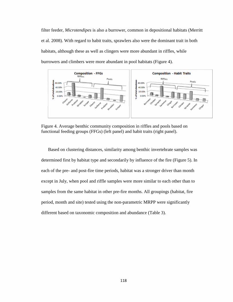
118

filter feeder, Microtendipes is also a burrower, common in depositional habitats (Merritt

et al. 2008). With regard to habit traits, sprawlers also were the dominant trait in both

habitats, although these as well as clingers were more abundant in riffles, while

burrowers and climbers were more abundant in pool habitats (Figure 4).

Figure 4. Average benthic community composition in riffles and pools based onfunctional feeding groups (FFGs) (left panel) and habit traits (right panel).

Based on clustering distances, similarity among benthic invertebrate samples was

determined first by habitat type and secondarily by influence of the fire (Figure 5). In

each of the pre- and post-fire time periods, habitat was a stronger driver than month

except in July, when pool and riffle samples were more similar to each other than to

samples from the same habitat in other pre-fire months. All groupings (habitat, fire

period, month and site) tested using the non-parametric MRPP were significantly

different based on taxonomic composition and abundance (Table 3).

119

Figure 5. Cluster analysis of benthic invertebrate samples from the East Fork JemezRiver, March to October 2011, color coded by habitat type (1=riffles, 2=pools). (Bray-Curtis distance metric, log (x + 1) abundance transformation, flexible beta = -0.25,percent chaining = 1.90).

Table 3. Multi-Response Permutation Procedure (MRPP) results comparing samplegroupings based on taxonomic composition.

Grouping T statistic A* p

Habitat -9.78 0.087 0.0000Fire -9.22 0.082 0.0000

Month -10.27 0.193 0.0000Site -2.57 0.055 0.0114

*chance-corrected group agreement

Indicator species analysis (ISA), used to investigate the taxa that were statistically

influential in determining habitat or pre- and post-fire community differences, showed

distinct groups of taxa that characterized riffles and pools, and a largely different group

of taxa that showed pre- and post-fire responses (Table 4).

120

Table 4. Indicator Values (IV) showing taxa significantly associated with cluster analysisgroupings: A. Habitat groupings of riffles (R) and pools (P); and B. Pre- and post-firegroupings.

A. Habitat (Riffle and Pool) Grouping

Taxon IV R (P) P Taxon IV P (R) p

Hydropsyche 87 (1) 0.0002 Enallagma 73 (5) 0.0008Heterolimnus 77 (17) 0.0002 Ephydridae 40 (0) 0.0164Helicopsyche 74 (8) 0.0004 Orthocladius 46 (6) 0.0296Acari 62 (35) 0.0010 Ameletus 45 (5) 0.0380Oecetis 63 (3) 0.0016 Physella 57 (40) 0.0496Tricorythodes 56 (44) 0.0016Bezzia 61 (10) 0.0068Hyalella 55 (45) 0.0104Simulium 48 (1) 0.0118Ophiogomphus 55 (15) 0.0306

B. Pre- and Post-Fire GroupingTaxon IV Pre (Post) P Taxon IV Post (Pre) p

Microtendipes 63 (34) 0.0002 Pentaneura 51 (5) 0.0122Orthocladius-Cricototopus

72 (0) 0.0002 Ostracoda 48 (6) 0.0200

Eukieferiella 72 (0) 0.0002 Tricorythodes 54 (46) 0.0242Hydrobaenus 61 (0) 0.0012 Microcylloepus 44 (2) 0.0212Fallceon 63 (13) 0.0044 Dubiraphia 59 (39) 0.0322Thiennemaniella 44 (0) 0.0090 Baetis 54 (17) 0.0464Hydroptilla 55 (6) 0.0178 Dytiscidae 25 (0) 0.0484Procladius 39 (0) 0.0260Ephydridae 33 (0) 0.0496

Even though the mayfly Tricorythodes is a sprawler, typical of depositional habitats,

and it occurs in both habitat types in the EFJR, it occurs in greater abundance and

frequency in riffles in the EFJR, and as a result has a high Indicator Value (IV) score at

riffle sites. While under natural conditions, Tricorythodes would be expected to increase

in abundance over the summer, its abundance remained relatively low through the period

of the fire until late in the fall (October), and therefore had a high indicator value for the

post-fire period.

121

The caddisflies Hydropsyche, Helicopsyche, Oecetis, and Hydroptilla, the elmid

beetle Heterlimnius, and the black fly Simulium, all clingers, were strongly associated

with riffle habitat (Table 4A). The amphipod Hyalella, another sprawler, and the

burrowers Bezzia (a dipteran) and Ophigomphus (a dragonfly) were also indicator species

for riffles.

Only a few taxa were significant indicator species of pools (Table 4A). These

included the damselfly Enallagma (a climber), brine flies in the family Ephidridae

(burrowers), the midge Orthocladius (a sprawler), the mayfly Ameletus (a swimmer), and

the snail Physella (a climber).

Indicator species values also showed which taxa were most characteristic of the pre-

and post-fire periods. Table 4B shows that six midge taxa (five sprawlers and one

burrower) and one mayfly (Fallceon, a swimmer), as well as Hydroptilla and Ephidridae,

were all common before the fire, and significantly less common after the fire. Several

taxa, including the sprawling midge Pentaneura, the small, shelled crustacean Ostracoda,

the mayfly Tricorythodes, the clinging elmid beetles Microcylloepus and Dubiraphia, the

swimming mayfly Baetis, and the predaceous diving beetles (Dytiscidae, swimmers),

were clearly more abundant and widely distributed in the post-fire period (Table 4B).

NMDS results corroborate the grouping of benthic samples based on habitat type and

fire period, and give insight into the environmental and habitat characteristics that drive

these groupings. The NMDS ordination based on taxonomic composition gave a

recommended 3-dimensional solution, with a final stress value of 12.64, well within the

optimal range of 20 or less (McCune and Grace 2002). Riffle and pool habitats separated

mainly on Axis 1, while pre- and post-fire periods separated on Axes 2 and 3 (Figure 6).

122

Axis 1 is correlated with water depth (negative) and velocity (positive), as well as with

the biomass and frequency of occurrence of the aquatic macrophytes Elodea (negative)

and Ranunculus (positive) (Table 5). Thus the composition of the benthic assemblages at

riffle sites were, in all months sampled, associated with higher velocities, shallower

depths, and the presence of Ranunculus, while pool assemblages were associated with the

deeper slower water and Elodea. The taxa that were significantly associated with the

riffle group (correlated positively with axis 1) included Heterlimnius, Tricorythodes,

Acari, and Helicopsyche (Table 6). These are consistent with the riffle indicator species

identified in association with cluster analysis, although it is not as extensive a list. Only

the damselfly Enallagma was significantly associated with pool sites in the NMDS

(Table 6).

Figure 6. Axes 1 and 2 from NMDS ordination using benthic invertebrate communitydata (3-dimensional solution recommended, final stress = 12.64), showing sampleshighlighted according to habitat (top 2 panels, 1=riffles, 2=pools), and association withthe Las Conchas fire (bottom 2 panels, 1=pre-fire, 2=post-fire). See Tables 5 and 6 forhabitat characteristics and taxa that define each axis.

123

Table 5. Correlation of habitat characteristic variables on each defining axis in NMDSordination (see Figure 6).

Axis 1 Axis 2 Axis 3Loading Variable r2 Variable r2 Variable r2

Positive

Velocity, max .57 DO, avg, interval .46 pH, min, interval .55Velocity, avg .40 PAR .68 DO, min, 2 wk .55

Ranunculus, biomass .37Ranunculus, freq .28

Negative

Depth, max .52 NO3, max, 2 wk .64 SC, avg, interval .47Depth, avg .50 PO4, avg, interval .52 Stage, max, interval .69

Elodea, freq .43 Temp, avg, interval .60 Flow, max, interval .43Elodea, biomass .30 pH, avg, interval .59 Turbidity, avg, 2 wk .40

pH, range, interval .52Turbidity, max, interval .59

DO, range, interval .63Precip, max, interval .83

Table 6. Correlation of benthic invertebrate taxa on each defining axis in NMDSordination (see Figure 6).

Axis 1 Axis 2 Axis 3Loading Variable r2 Variable r2 Variable r2

Positive

Heterlimnius .82 Ortho-Cricot .56 Hydroptila .60Hydropsyche .73 Thienemaniella .49 Tventenia .45Tricorythodes .47 Eukieferiella .38 Fallceon .43

Acari .37 Tipula .30 Microtendipes .40Helicopsyche .32 Graptocorixa .30 Psectrocladius .35

NegativeEnallagma .37 Dubiraphia .54 Enallagma .36

Ostracoda .31 Baetis .31

Axes 2 and 3 were correlated with variables that tracked precipitation inputs and

flow responses (stage, flow), as well as water quality and chemistry variables that

changed in association with these spates (Table 5). The benthic assemblages typical of

the pre-fire period grouped in the upper half of Axes 2 and 3, and were associated with

high average DO in the interval prior to sample collection, high PAR, higher minimum

pH and DO, as well as low precipitation and stage. The assemblages typical of the post-

fire period grouped in the lower half of Axes 2 and 3, and were correlated with high

124

maximum precipitation, stage and flow during the interval prior to benthic sample

collection, as well as peak values of NO3, PO4, turbidity, specific conductance (SC),

lower DO and pH minimums, and increased range (variability) in DO and pH (Table 5).

Benthic taxa that in the NMDS analysis were significantly associated with (more

abundant during) pre-fire conditions included the midges Orthocladius-Cricotopus,

Thienemaniella, Eukieferiella, Tventenia, Microtendipes, and Psectrocladius; the crane

fly Tipula, the water boatman Graptocorixa, the caddisfly Hydroptilla, and the mayfly

Fallceon (Table 6). This result is highly consistent with results of the ISA analysis (Table

4B). Species that were correlated with the post-fire period were Dubiraphia, Ostracoda,

Enallagma, and Baetis (Table 6). These taxa are again largely consistent with the post-

fire indicator species identified, although the ISA defined a slightly more extensive

group.

Benthic Invertebrate Trait Responses

Cluster analysis of the EFJR benthic communities based on composition of

Functional Feeding Groups (FFGs) was less effective than taxonomic composition in

differentiating riffle and pool habitats, although the MRPP showed habitats to be

significantly different based on FFGs (Table 7). Based on FFGs, riffles and pools mixed

at an intermediate distance (Figure 7). FFGs separated the benthic communities according

to the pre- and post-fire periods more strongly than habitat (Figure 7).

125

Table 7. Multi-Response Permutation Procedure (MRPP) results comparing samplegroupings based on Functional Feeding Group (FFG) composition.

Grouping T statistic A* p

Habitat -2.60 0.039 0.0230Fire -5.81 0.088 0.0004

Month -6.29 0.201 0.0000Site 0.19 -0.007 0.5429

*chance-corrected group agreement

Figure 7. Cluster analysis of benthic invertebrate samples from the East Fork Jemez Riverbased on composition of Function Feeding Groups (FFGs), March to October 2011, colorcoded by fire period (1=pre-fire, 2=post-fire). (Bray-Curtis distance metric, log (x + 1)abundance transformation, flexible beta = -0.25, percent chaining = 6.01).

Indicator values for FFGs showed that filterers and shredders were significantly

associated with the pre-fire period, while gathers were indicators of the post-fire period

(Table 8). Scrapers and predators showed no significant difference between periods based

on this indicator species analysis, which combines abundance and frequency of

occurrence metrics. However, when abundances were examined separately by habitat

126

type, scrapers, which were only slightly less abundant in riffles than pools before the fire,

only showed a substantial post-fire decline in abundance in the riffle habitat (Figure 8).

Although shredders were more abundant in pools pre-fire, a post-fire decline in

abundance occurred in both habitat types (Figure 8). This occurred despite the low

overall abundance of shredders in the EFJR, likely reflecting the lack of woody riparian

vegetation and associated litter input. Gatherers were more abundant after the fire in both

habitats, so the ISA analysis adequately documented their response. Filterers were

generally more abundant in pools, and showed a much bigger decline after the fire in

pools (Figure 8). Separating the analysis of fire responses by habitat may be important,

especially for the more specialized feeders (e.g., scrapers, filterers).

Table 8. Indicator Values (IV) showing Functional Feeding Groups (FFGs; collector-filterers, collector-gatherers, predators, shredders, scrapers) significantly associated withpre- and post-fire cluster groupings.

Pre-Fire Post-Fire

FFG IV Pre(Post)

P FFG IV Post (Pre) p

Filterers 55 (45) 0.0036 Gatherers 52 (48) 0.0418Shredders 52 (1) 0.0134

127

Figure 8. Average pre- and post-fire abundances of Functional Feeding Groups (FFGs)averaged separately by habitat type.

Cluster analysis of communities based on habit trait composition separated habitat

types (Figure 9), and this habitat grouping was significant based on MRPP (Table 9), but

the separation of habitat based on habit is not quite as strong as that based on taxonomic

composition. Habit traits do not separate the pre- and post-fire periods fire very well

(although the difference is significant in MRPP, Table 9).

Table 9. Multi-Response Permutation Procedure (MRPP) results comparing samplegroupings based on habit trait (burrowers, climbers, sprawlers, swimmers, clingers,divers, skaters) composition.

Grouping T statistic A* p

Habitat -7.76 0.106 0.0000Fire -2.16 0.295 0.0375

Month -4.10 0.118 0.0007Site -3.08 0.101 0.0045

*chance-corrected group agreement

128

Figure 9. Cluster analysis of benthic invertebrate samples from the East Fork Jemez Riverbased on composition of habit traits, March to October 2011, color coded by habitatperiod (1=riffle, 2=pool). (Bray-Curtis distance metric, log (x + 1) abundancetransformation, flexible beta = -0.25, percent chaining = 2.53).

Both clingers and sprawlers had significantly higher Indicator Values for riffles than

pools, while climbers were more strongly characteristic of pools than riffles (Table 10).

Only burrowers were a significant indicator group with regard to the fire (not shown),

with burrowers more abundant pre-fire than post-fire. A weakness of using ISA on trait

groups is that all five habit trait groups occur at all sites and sampling periods, so that the

frequency of occurrence is always 100%. Thus in the calculation of the IV, the

meaningful patterns in the habit types is in the abundance component of the metrics.

Overall, habit groups are stronger at separating habitat types than feeding groups, but

FFGs are better at distinguishing pre and post fire periods.

129

Table 10. Indicator Values (IV) showing habit traits (burrowers, climbers, sprawlers,swimmers, clingers, divers, skaters) significantly associated with habitat (R=riffle,P=pool) cluster groupings.

Riffles Pools

Habit IV* R (P) P Habit IV* P (R) p

Clingers 56 (44) 0.0002 Climbers 55 (45) 0.0080Sprawlers 52 (48) 0.0072

* Indicator Value = (abundance in group/sum of average abundances across all groups) *(# of samples of taxon present/total # samples)

If the average abundances of clingers and climbers, both strong indicators of habitat

types (riffles and pools, respectively), are separated by habitat type to compare pre- and

post-fire periods, it is clear there is no strong response to the fire by either of these trait

groups (Figure 10). Sprawlers and burrowers were both responsive to fire effects,

increasing in abundance post-fire in both habitat types (Figure 10). The magnitude of

response for the burrowers was much larger in pool habitats. Finally, swimmers

decreased in abundance post-fire, but only in the riffle habitat, even though the

abundance of swimmers was similar between habitat types before the fire (Figure 10).

130

Figure 10. Average pre- and post-fire abundances of habit trait groups averagedseparately by habitat type.

Given the evidence that scouring by post-fire flow pulses was influential in reducing

macrophyte biomass and potentially determining benthic invertebrate responses, the

responses of invertebrates classified based on their rheophily, or flow preference, traits

was examined. Depositional taxa were only slightly more abundant in pools compared to

riffles before the fire, which may be attributed to the embedding of riffles with finer

sediments found in the EFJR (Figure 11). After the fire, depositional taxa were less

abundant in pools than before the fire, but more abundant in riffles, suggesting

redistribution and deposition of fine sediments during post-fire flow events. Erosional

131

taxa, those that do well in higher flows, were more abundant in both habitat types after

the fire (Figure 11).

Figure 11. Average pre- and post-fire abundances of rheophily trait groups (preferencefor erosional or depositional conditions) averaged separately by habitat type.

Key Species Patterns

The abundance patterns of several key taxa show variable response patterns. EPT taxa

(Ephemeroptera-Plecoptera-Trichoptera) are often grouped to use as an indicator of

habitat condition, because they are considered sensitive to pollution and disturbance (note

that no Plecoptera were collected from our study area, so this group is only represented

by Ephemeroptera and Trichoptera). Riffle and pool differences in both abundance and

richness of EPT taxa are apparent (Figure 12). In both habitat types, EPT taxa increased

in abundance but decreased in richness after the fire. However, the abundance response

pattern was largely the result of a single taxon, the Ephemeropteran (mayfly)

Tricorythodes, which increased in abundance late in the year (October), after the fire, and

was a community dominant. Many other EPT taxa decreased in abundance in response to

the fire, in part reflected in the decreased number of EPT taxa post-fire. These species

differences in response are lost when examining EPT as a single indicator metric.

132

Figure 12. Average pre- and post-fire abundances and richness (number of taxa) of EPT(Ephemeroptera-Plecoptera-Trichoptera) and Chironomidae taxon groups, averagedseparately by habitat type.

The Chironomidae (non-biting midges) also are often examined as a group,

considered generally tolerant of organic pollution. However in this study, the

Chironomidae decreased in both abundance and richness in both habitats post-fire (Figure

12). All but one of the 21 genera identified also decreased in abundance post-fire

(Pentaneura increased slightly in abundance post-fire).

Discussion

The Las Conchas fire was a very large (63,000 hectare), moderate to severe wildfire

that burned much of the East Fork Jemez River watershed upstream and to the east of our

study site, without burning directly through the grassland site. Accordingly, although we

sampled in July during the burn period but before the onset of the summer monsoons, we

neither expected nor observed direct fire effects during that time. Even in streams with

133

riparian forests that are burned, direct effects from temperature (Mahlum et al. 2011),

ash-fall and the like, have been found to be minimal compared to subsequent indirect

effects (Minshall 2003, Minshall et al. 2001b, Rinne 1996). Our main focus was thus on

indirect, short-term effects of the fire on the EFJR benthic communities based on before-

after comparisons.

Unlike most of the forested streams studied for fire effects, the EFJR has an open

riparian canopy and good light penetration that supports strong macrophyte and

associated algal growth. It is seasonally dominated by aquatic macrophytes, with distinct

differences between pools and riffles in dominant species, with typically greater standing

stock biomass in pools (Table 1). There is substantial diatom and biofilm growth on riffle

substrates, as well as epiphytic diatoms on the macrophytes. The greater abundance of

epiphytic diatoms available in pools corresponds well with the greater occurrence of

invertebrate scrapers (=grazers) in pools compared to riffles. In addition, the nature of

trophic impacts of the fire can be expected to differ from those commonly found in other

forested streams with a well-developed riparian overstory and inputs of allochthonous

litter.

Water Quality Responses of the EFJR to the Fire

There were distinctive effects of the Las Conchas fire on the water quality of the

EFJR that we could document and link to post-fire runoff events at a fine temporal scale

not commonly possible due to the deployment of continuous real-time sensors. In-stream

responses in turbidity, DO, and pH are clearly associated with monsoon flow pulses that

followed the fire (Figure 13). The long period of record of continuously recorded data

134

during the pre-fire period documents the typically low turbidity of the EFJR, with a

characteristically low range of variability. Although both DO and pH showed expected

seasonal patterns during the first half of 2011 (e.g. increase in mean daily DO following

ice-off, steadily increasing pH from winter through the spring and early summer

reflecting increasing biological activity), the ranges of variation in daily mean DO and

pH were small and fairly consistent during that pre-fire period (Figure 13). Interestingly,

there was a significant rainstorm on June 24, just prior to the fire start, that had little

corresponding effect on runoff, and was associated with only a minor increase in turbidity

(<95 NTU). Over the period that the Las Conchas fire burned through the Valles Caldera

(early in the fire period shown by the red rectangle in Figure 13), during which there

were no major rainfall events, there were minimal if any water quality responses

observed, with the possible exception of a very small increase in the range of turbidity

variation that may reflect inputs of ashfall (though all daily means remained <90 NTU).

However, with the first major monsoon rainfall event following the fire (actually two

closely spaced events on August 3rd and August 6th), we observed distinct and rapid

responses (by August 4th and 7th respectively) in runoff and water quality. On these first

paired events, the increase in daily mean flow was modest (from a daily mean on August

3rd of 0.09 m3/s to 0.11 m3/s on August 4th, with similar magnitudes on August 6th and

7th). However, the increase in turbidity was distinct (from 22 to 340 NTU on the first

pulse, 23 to 228 NTU on the second pulse). There were associated pulse depressions in

mean pH (from about 9.3 to 7.4 on the first pulse, with a lesser change of 8.8 to 7.8 on

the second pulse), which also greatly reduced the daily range in pH, and in DO (to a daily

mean of 3 mg/l).

135

Figure 13. Daily values of mean flow, maximum turbidity, mean dissolved oxygen (DO),and maximum pH in the East Fork Jemez River during 2011. Sampling events areindicated by grey vertical lines. The red rectangle highlights the period of the LasConchas fire.

There were several subsequent significant monsoon rainfall events that were rapidly

followed by very high runoff pulses (e.g., an August 23rd flow pulse of about 0.63 m3/s

[approximately 7.6 times the pre-fire average flow rate], an August 28th and 29th pulse of

0.23 m3/s, and a September 6th pulse of 0.34 m3/s). Each of these runoff pulses were

associated with sharp increases in turbidity, to levels >1,000 NTU (Figure 13). Turbidity

is actually measured based on light scattering, and so is not always reliably associated

136

with suspended sediment load. Nevertheless, we believe the high turbidities are indicative

of the high levels of ash, suspended sediment, and charcoal that were eroded from the

watershed in these post-fire rainfalls and transported by each of these high-pulse flow

events in the EFJR both upstream of and within the study area (see Figure 14). Rapid

revegetation of the burned grasslands was observed within the VCNP, as illustrated in

Figure 15, suggesting that these eroded materials were not coming primarily from the

surrounding grasslands, but rather from the upstream, severely burned forested portions

of the EFJR watershed.

Figure 14. Photo upstream of the East Fork Jemez River study reach, taken in August2011 immediately following the Las Conchas fire, during a flow pulse resulting from amonsoon precipitation event, showing high flows with high loads of debris, ash, andsediment.

137

Figure 15. Photos of a Valles Caldera grassland area immediately after the Las Conchasfire burned through (July 6, 2011) and one month later (August 3, 2011) showing rapidrecovery of the grasslands.

Responses in other water quality parameters that are biologically significant were also

observed to be linked to these post-fire flow pulses. Sags in dissolved oxygen (DO)

occurred with each flow pulse, reducing DO to daily averages of about 3 mg/l that

persisted for two to three days (Figure 13). These sags included values below 6 mg/l, the

NMED standard for high-quality cold waters, for three to four days. During the August

22-24 event, all 15-minute interval DO measurements remained below 4 mg/l for the

entire 3-day period, with periods during the peak flows of DO below 3 mg/l, and often

down to 2.1 mg/l. Such extended periods of DO sags are likely to be biologically

stressful. Maximum pH values during this (and subsequent) pulse events were depressed

from about 9.4 to 7.4 (Figure 13). These lower pHs are still circumneutral, so it is not

clear whether this relatively large pH change would be directly stressful to

macroinvertebrates, or whether the pH response is an important indicator of pulse-

associated alterations in stream metabolism processes. Similar responses (not shown) in

major nutrients, respiration, and productivity also were observed (Sherson 2012, Shafer

2013). Many of these parameters were significantly associated with invertebrate

taxonomic and trait community responses to the fire. Several other studies have

documented a substantial increase in post-fire runoff associated with rain events

(Veenhuis 2002, Minshall et al. 1997, 2001a and b), post-fire changes in channel

morphology resulting from flow alterations (Benda et al. 2003), and impacts to benthic

and other aquatic communities that are mainly associated with post-fire flows (Minshall

2003, Earl and Blinn 2003, Rinne 1996). Few, however, have documented the close

138

linkages among rainfall and runoff pulse events and water quality parameters, nor the

temporal duration and severity of the water quality alterations. This study shows the

extent to which a fire of the severity of the Las Conchas burn can impact stream water

quality, linking severe fire impacts in the upper forested watershed to downstream water

quality impacts through pulsed monsoonal flow events affecting turbidity, DO, pH, and

nutrients.

Characteristics of the EFJR Benthic Communities

Our study catchment includes substantial areas of subalpine and mid-elevation

coniferous forests. About 63% of the EFJR catchment is forested (NMED 2009), but the

study stream reach itself runs through a broad, high-elevation meadow, and has no

natural woody riparian vegetation. Correspondingly, shredders comprise only a small

proportion of the community (0%-1.4%) in both habitats and all months. This is

somewhat low for a high elevation, second to third-order stream, but not inconsistent

with expectations for reduced shredder abundance in the transition from an allochthonous

to autochthonous energy base (Vannote et al. 1980, Cummins 1974). The dominance that

we observed in the EFJR by collectors (considering both gatherers and filterers),

averaging 70% of the fauna in pools and 80% in riffles (see Figure 4), is perhaps high

compared to the general expectations set by the River Continuum Concept (Vannote et al.

1980), and correspondingly, there are somewhat fewer scrapers (=grazers), averaging

about 24% of the fauna in pools and 12% in riffles, than would be expected in a system

like the EFJR with high autotrophic production. These patterns are difficult to explain,

and could reflect variation or uncertainty in assigning taxa to feeding types, or switching

139

in feeding mode with age, as well as the possibility that despite the high autochthonous

production, a substantial proportion of the energy base in this stream reach may come

from detritus washed into the stream from the surrounding grasslands, or from in-stream

processing of decomposing macrophyte material.

We found no stoneflies in our study reach of the EFJR, although stoneflies are a

common faunal component of the Jemez Mountains, as well as other mountain streams in

the west (e.g., Ward et al. 2002) and southwest (e.g., Molles 1985) and have been

collected from upstream reaches of the EFJR. Many stoneflies are shredders, and many

are considered cold-preference taxa, so their exclusion from the study reach could reflect

responses to the condition of these factors in the EFJR. The EFJR in the vicinity of the

study area was listed in 2001 as exceeding water quality standards for its designated use

(high quality cold water aquatic life) for temperature (temperature of 20°C not to be

exceeded for four or more consecutive hours in a 24-hour period on more than three

consecutive days or a maximum temperature of 23oC), as well as for pH (range of 6.6 to

8.8), DO (minimum of 6.0 mg/l), turbidity (no increase >10 NTU when background is

<50 NTU), and coliforms (the monthly geometric mean of E. coli bacteria 126 cfu/100

mL or less, single sample 235 cfu/100 mL or less) by the New Mexico Environment

Department (NMED) (Simino 2002). Based on monitoring in 2005 by NMED, the EFJR

was again listed as impaired for temperature as well as arsenic (NMED 2009). Simino

(2002) specifically sites the legacy of grazing impacts as contributing to higher

temperatures, because undercut banks that are lost due to trampling and increased erosion

would normally contribute shaded habitat and lower water temperatures. Flow velocities

also decrease with grazing and erosion, which contributes to increasing water

140

temperatures, while protection from grazing results in recovery of the stream profile and

increasing flow velocities (Van Horn et al. 2012). NMED indirectly recognizes the lack

of shading and increased stream width as contributing to higher temperatures (NMED

2009). These existing water quality degradations, as well as the very low gradient of the

stream, may contribute to the absence of stoneflies in the study area. There are other

faunal differences between our EFJR study reach and other high-elevation streams in

New Mexico. For example, there is essentially no overlap in the genera of Trichoptera

(caddisflies) collected in the EFJR and those reported by Molles (1982) for two forested,

first to second order streams in the southern Sangre de Cristo Mountains. This could

reflect zoogeographic faunal differences between the Jemez and Sangre de Cristo

mountain ranges, in addition to differences expected between forested and open canopy

streams.

Some evidence suggests that the riffles and pools in the EFJR may not be

differentiated to the extent that would be expected under undisturbed conditions. The

EFJR has a history of grazing (as well as logging) disturbance within the Valles Caldera

(Maldavin and Tonne 2003, Anschuetz and Merlan 2007) that results in widening and

shallowing of the stream profile, erosion of stream banks including loss of undercut

banks, and increased sediment runoff that fills in pools and embeds the gravel to cobble

riffle substrates. In a 2001 survey of the EFJR, Simino (2002) found conditions in the

upper reaches of the EFJR to reflect this type of disturbance, with eight times more riffle

than pool habitat due to sediment infilling, stream widening, and loss of sinuosity. Simino

(2002) also attributes the loss of pool habitat to the lack of large woody debris, which

contributes to pool formation through induction of local scour. Large woody debris is

141

absent in the study reach of the EFJR within the Valles Caldera, given the lack of riparian

forest in this area. Despite these reported conditions, we were able to differentiate riffles

and pool in the EFJR study area, based on geomorphic and hydrologic characteristics, to

a degree that proved useful in assessing fire effects on the benthic communities in these

habitats. Few studies on the effects of fires on stream benthic communities have

examined responses separately by riffle and pool habitat types (but see Earl and Blinn

2003).

Before and After Sampling of Invertebrates in a Fire-Impacted Stream

Most studies of fire effects on stream invertebrates, with the exception of prescribed

burn studies (e.g., Beche et al. 2005), rely on comparisons between burn-area streams and

reference streams (e.g., Minshall 2001a and b, 2003, Spencer et al. 2003). In contrast, we

had established a suite of in situ, continuous monitoring instruments examining

hydrology, water quality, and water chemistry, as well as regular biological monitoring

during the year, when the Las Conchas fire burned through and created the opportunity to

examine fire effects and responses within the same stream based on pre- and post-fire

comparisons. Another study in Yellowstone Park (Tronstad et al. 2011, 2013) also

fortuitously sampled benthos in Cub Creek in 2003, just before the East Fire in 2003 and

then one, two, and nine years thereafter. Rinne (1996) also sampled benthos (and fish) in

three streams in Arizona before and after the Dude Fire in 1990. In both of these cases,

the pre-fire sampling occurred a year before the fire incident, while in this study, pre- and

post-fire sampling represented a regular series of approximately 6-week interval samples

within one year.

142

After several pulse flow events that occurred in the EFJR immediately following the

Las Conchas fire, many vulnerable taxa were reduced in abundance, altering the post-fire

composition of invertebrate communities. However, there were no significant reductions

in the total abundance of benthic invertebrates in pools, and density increased somewhat

in riffles (Figure 16). In contrast to this, Tronstad et al. (2011, 2013) found the total

density of invertebrates decreased in Cub Creek the year following the East Fire, with

recovery to pre-fire densities in two years. However, they found that biomass was similar

before and after the fire, and increased in subsequent years. In the smaller Little Cub

Creek watershed, both density and biomass of invertebrates increased following the fire.

In three streams in the Gila watershed in Arizona, Rinne (1996) found no differences in

invertebrate density between pre-fire and immediate post-fire conditions prior to flooding

events, while after storm-related post-fire flood flows, densities of invertebrates were

significantly reduced (by up to 95%). The common theme is the linkage through the

timing of storm-associated runoff and fire severity, combined with factors that further

modify responses, such as land slope and stream gradient. When there were no major

pulse flows following the fire (e.g., Little Cub Creek, Tronstad et al. 2013), or before

such flows occurred (e.g., the Gila streams, Rinne 1996), minimal responses from the

invertebrate communities occurred. When flow pulses occurred after a fire, the

magnitude of benthic responses appeared to be greatest when flows transformed the

channels, or flows transport, scoured, and deposited large amounts of materials, including

toxic ash in transport (Rinne 1996). Earl and Blinn (2003) also observed reductions in

abundance of >95% following a large fire in the West Fork Gila River, attributed largely

to substantial ash inputs from the burned watershed.

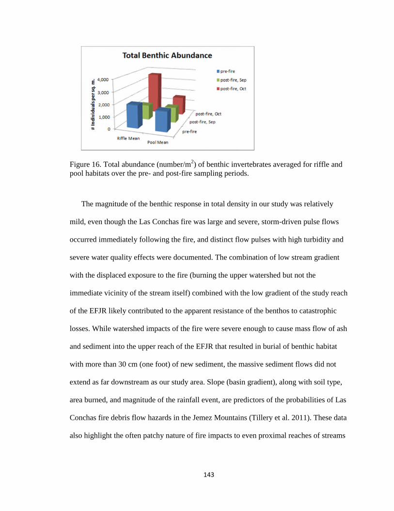
143

Figure 16. Total abundance (number/m2) of benthic invertebrates averaged for riffle andpool habitats over the pre- and post-fire sampling periods.

The magnitude of the benthic response in total density in our study was relatively

mild, even though the Las Conchas fire was large and severe, storm-driven pulse flows

occurred immediately following the fire, and distinct flow pulses with high turbidity and

severe water quality effects were documented. The combination of low stream gradient

with the displaced exposure to the fire (burning the upper watershed but not the

immediate vicinity of the stream itself) combined with the low gradient of the study reach

of the EFJR likely contributed to the apparent resistance of the benthos to catastrophic

losses. While watershed impacts of the fire were severe enough to cause mass flow of ash

and sediment into the upper reach of the EFJR that resulted in burial of benthic habitat

with more than 30 cm (one foot) of new sediment, the massive sediment flows did not

extend as far downstream as our study area. Slope (basin gradient), along with soil type,

area burned, and magnitude of the rainfall event, are predictors of the probabilities of Las

Conchas fire debris flow hazards in the Jemez Mountains (Tillery et al. 2011). These data

also highlight the often patchy nature of fire impacts to even proximal reaches of streams

144

(recognized in Minshall 2003), based on factors such as locally variable topographic

features, and spatially variable rainfall patterns within a region.

Even though the response in total density of invertebrates was moderate in the EFJR,

there were compositional changes in response to the fire in both pools and riffles.

Tronstad et al. (2011, 2013) found variable changes in composition among taxonomic

groups – ephemeropterans (mayflies) showed no net before-after change, trichopterans

decreased in density, and plecopterans (stoneflies) increased. But within these groups,

they found species differences (e.g., the mayflies Rhithrogenia and Plauditis increased

following the fire, while Serratella decreased). We also found species differences in

responses among the EPT taxa of the EFJR. The dominant mayflies Tricorythodes and

Baetis both decreased initially following the fire, and then increased later in the fall,

showing post-fire recovery. Other mayflies such as Fallceon decreased in abundance

post-fire in both habitat types, although they also started to show recovery in October;

and Ameletus increased in abundance post-fire. Among the caddisflies in the EFJR,

Helicopsyche and Hydroptila were significantly associated with (more abundant during)

the pre-fire period, while Hydropsyche increased post-fire (though not significantly).

Tronstad et al. (2011) suggested that the variable EPT response was evidence that the

responses were not related to water quality, but rather to resistance to floods and

tolerance to increased levels of fine sediments. Based on our observations of the recovery

trajectories of the mayflies that responded to fire effects (initial large abundance

decreases in September immediately following the post-fire pulse flows, followed by

increases in abundance one month later), we would suggest that their opportunistic life

history characteristics provide a mechanism for post-fire resilience. For example,

145

Tricorythodes, which has extended reproduction and recruitment throughout the summer

rather than a highly synchronized period of reproduction, and Baetis, which is bivoltine,

both began recovering in abundance in the fall immediately after the monsoon season. In

contrast, Helicopsyche, which is univoltine with emergence in spring and larval growth

and highest densities in summer, remained reduced in abundance throughout the fall. As

a clinger on rock surfaces in riffles (erosional environments), Helicopsyche was

vulnerable to scouring during the post-wildfire pulse-flow episodes, and since these

occurred after their main recruitment period, there was little opportunity for immediate

recovery.

Tronstad et al. (2013) found that the true flies in the family Chironomidae (midges)

increased in Little Cub Creek after the East Fire, and attributed this to their

characterization as tolerant taxa. In contrast, we found all genera of Chironomidae that

occurred in the EFJR, with the exception of the predaceous tanypod Pentaneura, to

decrease following the Las Conchas fire, with no recovery yet apparent in the fall of

2011. Given the diverse combination of midges that occurred in the EFJR (20 genera,

multiple feeding and life history types), it is not likely that strategies adaptive to the types

of fire disturbances observed are common among all of them. As a result, we suggest that

tracking chironomids as a singular group would not be informative for assessing the

physical and water quality disruptions that the Las Conchas and other fires generate.

Functional Trait Responses to the Las Conchas Fire

Although Mihuc et al. (1996) found that benthic invertebrate responses were

individualistic, there is value in investigating whether some combinations of species traits

146

and habitat conditions may increase the vulnerability of taxa to post-fire effects, and

provide predictive power with regard to future and long-term effects. The effects of the

Las Conchas fire on the EFJR can be grouped into two different though inter-related

categories of disturbance, direct physical disruption, in which we could include direct

water quality and trophic impacts. In general, we expected the scouring and sediment

deposition associated with post-fire flow pulses to be most likely to generate observable

effects within the immediate post-fire timeframe of our study. We hypothesized that life

history traits that imparted resistance to dislodgement in strong flows, such as clinging or

sprawling habits, or erosional versus depositional rheophily preference, would provide

predictive categories to track these physical disturbances. On the other hand, we expected

trophic effects of the fire would likely take longer for associated invertebrate changes to

manifest in terms of community composition. Although different from most other fire

study cases because of the pre-fire open canopy of the EFJR, we expected trophic

impacts of the fire to be potentially important but in the longer term. For instance, the

loss in macrophyte biomass due to the immediate post-fire scouring pulse flows, the

associated loss of epiphytes, and the additional scouring of other (e.g., episammic)

diatoms represent a substantial loss of food resources for invertebrates, which could

contribute to restructuring of the benthic community. We tested these by tracking the

responses of functional feeding types.

Despite expectations, our traits-based community analyses combined with pre- and

post-fire abundance patterns by trait groups showed that habit traits were not as effective

as functional feeding groups at separating the pre-and post-fire periods. Community

composition by habit traits effectively separated riffle and pool habitats, but functional

147

feeding groups were more responsive to fire effects within habitat type. This suggests that

within the three month post-fire period during which sampling was conducted (August to

October), fire-related alterations of EFJR trophic resources influenced the composition of

the benthic community.

Tronstad et al. (2011) also postulated that benthic food webs in streams would be

altered by fire-induced changes to light levels, nutrient concentrations, and hydrology. It

should be noted, however, that the expectation for most streams impacted by severe,

stand-replacing fires is for a shift from heterotrophy toward a greater contribution to the

energy base by autotrophy. This results from a combination of changes, including the

opening of the forest canopy, increased light penetration to support primary production,

loss of leaf litter inputs, and increased nutrient inputs. This leads to an expectation for a

decrease in shredder abundance and an increase in scraper (herbivore) abundance as a

response to decreased leaf litter input and increased algal production following a fire in

the near (Minshall 2003) or long-term (Molles 1982). In forested stream case studies, the

expected response of feeding types was not consistently observed (Minshall 2003). For

example, Tronstad et al. (2011) found that shredders increased in abundance and biomass

after the East Fire in Yellowstone, while scraper abundance decreased slightly in the year

following the fire, and recovered in the second post-fire year. However, scraper biomass

did increase in the year following the fire, consistent with expectations. In contrast, the

EFJR already had a substantial autotrophic energy base. Many of the watershed inputs are

similar to other forest fire-impacted streams, including altered hydrology, erosion, and

nutrient inputs. However, the short-term trophic changes are at first related to the loss of

148

autotrophs and depression of production rather than to a shift from a heterotrophic

resource base.

When examined separately by habitat type, benthic responses to the fire based on

functional feeding groups were apparent. Scrapers were strongly impacted in riffles,

although not in pools, indicating greater vulnerability to post-fire scouring effects in

riffles. While this was consistent with the reduction in abundance of their food resource,

we explored whether the immediate post-fire loss of scrapers was due to the loss of their

trophic resource (epiphytes) or to dislodgment in scouring flows plus the loss of the

habitat structure by comparing pre- and post-fire responses of habit traits instead of

feeding types. In the EFJR, scraper taxa are represented by a variety of habit traits

including climbers, clingers, swimmers, and one sprawler. However, neither the

abundance of climbers (often associated with macrophytes) or of clingers (on rocks,

macrophytes, other substrates) declined post-fire. Gatherers are a more general feeding

type and are often considered opportunistic, and their greater abundance post-fire is

consistent with other fire study results that found opportunists to respond well after fire

impacts on streams (Mihuc et al. 1996, Minshall 2003).

Evaluation of habit (i.e., mode of habitat use) traits did highlight invertebrate

vulnerabilities that were consistent with the main physical disturbances created by the

fire. Within the riffle habitat, swimmers were vulnerable and declined in abundance,

presumably reflecting the greater exposure to scour that might be expected in riffles.

Burrowers were particularly impacted in pools, although not in riffles, highlighting the

potential for peak flow events to scour soft sediments from the pools, and subsequently to

deposit transported sediments during recession. However, short-term recovery potential

149

was not defined by these habitat traits, but rather by the possession of opportunistic

reproductive habits that allowed recruitment to occur rapidly following cessation of the

large, flashy pulse flows with high turbidity. Species characterized as opportunistic are

found to respond favorably after fires (Minshall 2003).

Short-Term Effects, Long-Term Expectations

Historical (pre-1900) fire return intervals averaged 5 to 25 years in the Jemez

Mountains, or a watershed-wide fire every 16 years on average (Allen 2002a). Fires were

most frequent in mid-elevation ponderosa pines, and periods of fire activity were found to

be associated with periods of drought (Allen 2002a). During the twentieth century, fire

suppression practices as well as increased grazing altered fire frequency, and resulted in

shifts from open forests to dense thickets of smaller trees in the Jemez Mountains,

increasing the likelihood and intensity of crown fires, which often result in replacement

of the forest with shrublands (Allen 2002a, Allen 1989). The shift to more susceptible

landscapes, combined with climate change effects that are increasing aridity in the

Southwest (Seager et al. 2007, Gutzler and Robbins 2010), has increased the frequency of

stand-replacing fires in the Southwest (e.g., Swetnan and Betancourt 1998, Bachelet et al.

2007). This trend is expected to continue (Running 2006, Westerling et al. 2006). Burned

watersheds have altered runoff, erosion, and in-stream flow characteristics that can

persist (Robichaud et al. 2000) and cause moderate to traumatic alteration of stream

invertebrate communities in the short-term (this study, Minshall 2003, Earl and Blinn

2003, many others). A more frequent recurrence of such traumatic disturbance of

montane stream communities can thus be expected in the near term. Disturbance is

150

recognized as an important factor organizing the structure of stream communities (Resh

et al. 1988), but the responses to such restructuring will depend on factors such as the

frequency and intensity of the disturbance, the timing of the disturbance relative to the

life histories of the resident organisms, and hydrologic characteristics of the stream

driven by factors such as regional climate, topography, and geomorphology (Resh et al.

1988). If stream invertebrate community attributes of abundance, species richness, and

diversity in burned streams take 10-15 years to return to ‘normal’ and converge with the

values of community attributes from reference (unburned) streams (see Minshall 2003 for

summary of pertinent evidence), then major fire disturbances more frequent than an

average of once every 16 years should allow disequilibria to persist. Our study results

suggest these could include, for example, repeated suppression of certain feeding types

such as scrapers. In the absence of fire disturbance, scrapers are sub-dominants in the

EFJR, exploiting the abundant autotrophic resources (epiphytic and episammic diatoms).

As fire disturbances occur at intervals shorter than observed community recovery times,

scrapers may not return to their pre-fire sub-dominant status, despite the availability of

exploitable trophic resources. Similarly, we would postulate that taxa with more extended

reproduction and recruitment periods or other opportunistic reproduction characteristics

would be favored by a higher return rate of fire disturbance. Thus, an increasing fire and

associated flow disturbance frequency could result in persistent shifts in benthic

community composition and function. While less severe fire disturbances can have

minimal effects on benthic communities, with recovery to pre-fire or reference conditions

within periods as little as one year (Beche et al. 2005, Earl and Blinn 2003), severe fire

disturbance to the watershed that results in traumatic flow disturbance may result in

151

alterations to the benthic community that are not rapidly recovered and persistent (Arkle

et al. 2010).

Overall, we found that responses of stream benthic invertebrates to a major fire

disturbance in the EFJR reflected three categories, vulnerability, resistance, and

resilience, with different groups of organisms and different trait characteristics

comprising each. Even in the short term, vulnerability was observed to both direct

physical disturbance, mediated by the flow pulses that followed the fire; and to trophic

impacts, that were secondary responses to loss of food resources due to those same flow

pulses and associated water quality effects. Resistance to the post-fire physical

disturbance of the stream environment was exhibited by a subset of invertebrates with

habit traits such as climbers and clingers, that conferred the ability to withstand

dislodgement and displacement that would otherwise be expected from the post-fire flow

pulses. Resilience, or ability to recover in the short term following cessation of the most

prominent post-fire flow events, was conferred mainly by opportunistic life-history traits.

This suite of responses suggest the mechanisms through which benthic communities may

be altered in the long-term, through suppression of some vulnerable taxa, partial if not

temporary (short-term) suppression of some trophic resources, and possibly incomplete

recovery (relative to pre-fire conditions) based on the reproductive life-history

characteristics of component taxa.

152

References

Allen, C.D. 1989. Changes in the Landscape of the Jemez Mountains, New Mexico.Ph.D. dissertation, University of California, Berkeley, CA. 346 pp.

Allen, C.D. 2007. Interactions across spatial scales among forest dieback, fire, anderosion in northern New Mexico landscapes. Ecosystems 10:797-808.

Allen, C.D. 2002a. Fire and vegetation history of the Jemez Mountains. USGS FortCollins Science Center, Jemez Mountains Fields Station, Los Alamos, NM. 10 pp.

Allen, C.D. 2002b. Lots of lightning and plenty of people: An ecological history of fire inthe upland Southwest. p. 143-193 in: T.R. Vale (ed.), Fire, Native Peoples, and theNatural Landscape. Island Press, Covelo, CA.

Anschuetz, K.F. and T. Merlan. 2007. More Than a Scenic Mountain Landscape: VallesCaldera National Preserve Land Use History. United States Department ofAgriculture, Forest Service, Rocky Mountain Research Station. General TechnicalReport RMRS-GTR-196. 289 pp.

Bachelet, D., J.M. Lenihan, and R.P. Neilson. 2007. Wildfires and global climate change:the importance of climate change for future wildfire scenarios in the western UnitedStates. Prepared for the Pew Center on Global Climate Change. 28 pp.

Beche, L., S.L. Stephens, and V.H. Resh. 2005. Effects of prescribed fire on a SierraNevada (California, USA) stream and its riparian zone. Forest Ecology andManagement 218:37–59.

Benda, L., D. Miller, P. Bigelow, and K. Andras. 2003. Effects of post-wildfire erosionon channel environments, Boise River, Idaho. Forest Ecology and Management178:105–119.

Boesch, D.F. 1977. Application of numerical classification in ecological investigations ofwater pollution. Ecological Research Series, EPA-600/3-77-033. U.S. EPA Office ofResearch and Development, Corvallis, Oregon. 126 pp.

Bray, J. R. and J. T. Curtis. 1957. An ordination of upland forest communities of southernWisconsin. Ecological Monographs 27: 325-349.

Cannon, S.H., J.E. Gartner, M.G. Rupert, J.A. Michael, A.H. Rea, and C. Parrett. 2010.Predicting the probability and volume of post-wildfire debris flows in theintermountain western United States. Geological Society of America Bulletin122(1/2):127–144. doi: 10.1130/B26459.1.

Cummins, K.W. 1974. Structure and function of stream ecosystems. BioScience24(11):631-641.

153

Cummins, K.W. and M.J. Klug. 1979. Feeding ecology of stream invertebrates. AnnualReview of Ecology and Systematics 10:147-172.

Dufrene, M. and P. Legendre. 1997. Species assemblages and indicator species: the needfor a flexible asymmetrical approach. Ecological Monographs 67:53-73.

Earl, S.R. and D.W. Blinn. 2003. Effects of wildfire ash on water chemistry and biota inSouth-Western U.S.A. streams. Freshwater Biology 48:1015–1030.

Franklin, J.F. and M.A. Hemstrom. 1981 Aspects of succession in the coniferous forestsof the Pacific Northwest. p. 212-229 In: D.C West, H.H. Shugart, and D.B. Botkin,(eds.) Forest Succession: Concepts and Application. New York: Springer-Verlag.

Gallaher, B.M. and R.J. Koch. 2005. Water Quality and Stream Flow After the CerroGrande Fire: A Summary. Los Alamos National Laboratory, LALP-05-009. 46 pp.

Griffith, G.E., J.M. Omernik, M.M. McGraw, G.Z. Jacobi, C.M. Canavan, T.S. Schrader,D. Mercer, R. Hill, and B.C. Moran. 2006. Ecoregions of New Mexico (color posterwith map, descriptive text, summary tables, and photographs): Reston, Virginia, U.S.Geological Survey (map scale 1:1,400,000).

Gutzler, D.S. and T.O. Robbins. 2010. Climate variability and projected change in thewestern United States: regional downscaling and drought statistics. ClimateDynamics 37:835–849. DOI 10.1007/s00382-010-0838-7.

Johnson, E.A. 1992. Fire and vegetation dynamics. Cambridge University Press,Cambridge, UK.

Mahlum, S.K., L.A. Eby, M.K. Young, C.G. Clancy, and M. Jakober. 2011. Effects ofwildfire on stream temperatures in the Bitterroot River Basin, Montana. InternationalJournal of Wildland Fire 20:240–247.

McCune, B. and J.B. Grace. 2002. Analysis of Ecological Communities. MJM SoftwareDesign, Gleneden Beach, Oregon. 300 pp.

McCune, B. and M. J. Mefford. 2006. PC-ORD. Multivariate Analysis of EcologicalData. Version 5.18. MjM Software, Gleneden Beach, Oregon, U.S.A.

Merritt, R.W., K.W. Cummins, and M.B. Berg. 2008. An Introduction to the AquaticInsects of North America. Fourth Edition. Kendall/Hunt Publishing Company,Dubuque, Iowa. 1158 pp.

Mihuc, T.B., G.W. Minshall, and C.T. Robinson. 1996. Response of benthicmacroinvertebrate populations in Cache Creek, Yellowstone National Park to the1988 wildfires. pp. 83–94 In: Greenlee, J.M. (ed.). The Ecological Implications ofFire in Greater Yellowstone. International Association of Wildland Fire, Fairfield,Washington.

154

Mihuc, T.B. 2004. Food web dynamics in Yellowstone streams: shifts in the trophic basisof a stream food web after wildfire disturbance. Pages 189-199 in L. Wallace (ed.).After the Fires: The Ecology of Change in Yellowstone National Park. YaleUniversity Press, New Haven.

Miller, J.D., H.D. Safford, M. Crimmins, and A.E. Thode. 2009. Quantitative evidencefor increasing forest fire severity in the Sierra Nevada and southern CascadeMountains, California and Nevada, USA. Ecosystems 12:16-32. DOI:10.1007/S10021-008-9201.

Minshall, G.W. 2003. Responses of stream benthic macroinvertebrates to fire. ForestEcology and Management 178:155–161.

Minshall, G.W., T.V. Royer, and C.T. Robinson. 2001a. Response of the Cache Creekmacroinvertebrates during the first 10 years following disturbance by the 1988Yellowstone wildfires. Canadian Journal of Fisheries and Aquatic Science 58:1077–1088.

Minshall, G.W., C.T. Robinson, D.E. Lawrence, D.A. Andrews, and J.T. Brock. 2001b.Benthic macroinvertebrate assemblages in five central Idaho (USA) streams over a10-year period following disturbance by wildfire. International Journal of WildlandFire 10:201–213.

Minshall, G.W., C.T. Robinson, and D.E. Lawrence. 1997. Immediate and mid-termresponses of lotic ecosystems in Yellowstone National Park, USA to wildfire.Canadian Journal of Fisheries and Aquatic Sciences 54:2509–2525.

Molles, M.C., 1985. Recovery of a stream invertebrate community from a flash flood inTesuque Creek. The Southwestern Naturalist 30(2):279-287.

Molles, M.C. 1982. Trichopteran communities of streams associated with aspen andconifer forests: Long-Term structural change. Ecology 63(1):1-6.

Muldavin, E., and P. Tonne. 2003. A vegetation survey and preliminary ecologicalassessment of Valles Caldera National Preserve, New Mexico. Final Report underCooperative Agreement No. 01CRAG0014, the University of New Mexico and theU.S. Geological Survey, Biological Resources Division, Albuquerque, NM, USA.118 pp.

New Mexico Environment Department (NMED). 2009. WQCC-approved draft totalmaximum daily load (TMDL) for the Jemez River watershed. 179 pp.

Parmenter, R. 2011. The Las Conchas Fire: Flames and Floods in the Valles Caldera. LaVentana en los Valles – News of the Valles Caldera National Preserve from theValles Caldera Trust. Fall 2011.

155

Resh, V.H., A.V. Brown, A.P. Covich, M.E. Gurtz, H.W. Li, G.W. Minshall, S.R. Reice,A.L. Sheldon, J.B. Wallace, and R.C. Wissmar. 1988. The role of disturbance instream ecology. Journal of the North American Benthological Society 7:433–455.

Rinne, J.N. 1996. Short-term effects of wildfire on fishes and aquatic macroinvertebratesin the southwestern United States. North American Journal of Fisheries Management16:653–658.

Robichaud, P.R., J.L. Beyers, and D.G. Neary. 2000. Evaluating the effectiveness ofpostfire rehabilitation treatments. USDA Forest Service General Technical ReportRMRS-GTR-63. Fort Collins, Colorado.

Running, S.W. 2006. Is global warming causing more, larger wildfires? Science313(5789): 927-928.

Scholl, A.E. and A.H. Taylor. 2010. Fire regimes, forest change, and self-organization inan old-growth mixed-conifer forest, Yosemite National Park, USA. EcologicalApplications 20(2):362–380.

Seager, R., M. Ting, I. Held, Y. Kushnir, J. Lu, G. Vecchi, H.-P. Huang, N. Harnik, A.Leetmaa, N.-C. Lau, C. Li, J. Velez, and N. Naik. 2007. Model projections of animminent transition to a more arid climate in southwestern North America. Science1181-1184. [DOI:10.1126/science.1139601.

Shafer, B. 2013. Multi-Year Measurement of Whole-Stream Metabolism in a Snowmelt-Dominated Montane Ecosystem. Professional Project, Water Resources Program, TheUniversity of New Mexico Albuquerque, New Mexico. 48 pp.

Shapiro, S.S. and M.B. Wilk. 1965. An analysis of variance test for normality (completesamples). Biometrika 52 (3-4):591–611. doi:10.1093/biomet/52.3-4.591.

Sherson, L. 2012. Nutrient Dynamics in a Headwater Stream: Use of Continuous WaterQuality Sensors to Examine Seasonal, Event, and Diurnal Processes in the East ForkJemez River, NM. M.S. Thesis, Earth and Planetary Sciences, The University of NewMexico, Albuquerque, New Mexico. 91 pp.

Simino, J. 2002. East Fork Jemez River Stream Inventory Report. Santa Fe NationalForest, Jemez Ranger District. Surveyed July to September 2001. 75 pp.

Southwood, T.R.E. 1977. Habitat, the templet for ecological strategies? Journal ofAnimal Ecology 46:337-365.

Southwood, T.R.E. 1988. Tactics, strategies and templets. Oikos 52:3-18.

Spencer, C.N., K.O. Gabel, and F.R. Hauer. 2003. Wildfire effects on stream food websand nutrient dynamics in Glacier National Park, USA. Forest Ecology andManagement 178:141–153.

156

Swetnam, T.W. and J.L. Betancourt. 1998. Mesoscale disturbance and ecologicalresponse to decadal climatic variability in the American Southwest. Journal ofClimate 11:3128-3147.

Tillery, A.C., M.J. Darr, S.H. Cannon, and J.A. Michael. 2011, Post-wildfire preliminarydebris flow hazard assessment for the area burned by the 2011 Las Conchas Fire innorth-central New Mexico: U.S. Geological Survey Open-File Report 2011–1308. 11pp.

Tronstad, L.M., J.C. Bish, R.O. Hall, and Todd M. Koel. 2011. Comparing streaminvertebrate assemblages before and after wildfire in Yellowstone National Park.Report prepared by the Wyoming Natural Diversity Database for the YellowstoneNational Park. 6 pp.

U.S. Environmental Protection Agency (EPA). 2012. Freshwater Traits Database. GlobalChange Research Program, National Center for Environmental Assessment,Washington, DC; EPA/600/R-11/038F. Available from the National TechnicalInformation Service, Springfield, VA, and online at http://www.epa.gov/ncea.

Van Horn, D.J., C.S. White, E.A. Martinez, C. Hernandez, J.P. Merrill, R.R. Parmenter,and C.N. Dahm. 2012. Linkages between riparian characteristics, ungulate grazing,and geomorphology and nutrient cycling in montane grassland streams. RangelandEcology and Management 65:475–485.

Vannote, R.L., G.W. Minshall, K.W. Cummins, J.R. Sedell, and C.E. Cushing. 1980. Theriver continuum concept. Canadian Journal of Fisheries and Aquatic Sciences 37:130-137.

VCNP. 2012. Valles Caldera National Preserve. About VCNP. 15 March 2012.Available: http://www.vallescaldera.gov/about.

Veenhuis, J.E. 2002. Effects of wildfire on the hydrology of Capulin and Rito de LosFrijoles canyons, Bandelier National Monument, New Mexico. U.S. GeologicalSurvey Water Resources Investigation Report 02-4152. Available atnm.water.usgs.gov/publications/abstracts/wrir02-4152.pdf.

Ward, J.V., B.C. Kondratieff, and R.E. Zuellig. 2002. An Illustrated Guide to MountainStream Insects of Colorado. Second Edition. University Press of Colorado. Boulder,Colorado. 219 pp.

Westerling, A.L., H.G. Hidalgo, D.R. Cayan and T.W. Swetnam. 2006. Warming andearlier spring increase western U.S. forest wildfire activity. Science 313(5789):940-943.

Woodhouse, B. 2004. Fire effects on stream discharge. Southwest Hydrology,September/October 2004:22-23.

157

CHAPTER 5

Summary

This dissertation is about increasing our understanding of how climate changes and

extreme events affect stream invertebrate communities, with the goal of linking this

understanding to how stream invertebrates are used as bioassessment indicators and

responders to disturbance. Invertebrates are widely used as tools to assess conditions

within stream ecosystems, and as well, the process of bioassessment is widely applied in

the U.S. and around the world for resource management to determine the ecological

consequences of environmental stressors. Woodward et al. (2009) expressed concern

about the ability of biomonitoring to discern and account for degradation due to novel

stressors using procedures and indices developed under a system that focused on

documentation of organic pollution. This dissertation sought to further our

comprehension of how a novel stressor – climate change – and associated extreme events

influence stream benthic communities and the metrics and indicators we derive from

them, in a way that helps us advance the development of specific strategies to ensure the

long-term effectiveness of stream monitoring and management plans.

Chapter 1 introduced expectations for climate changes and how they relate to

stream ecosystems, as well as the basic concepts of bioassessment, as background for

why the influences of such a major environmental driver should be accounted for in terms

of its effects on the components of bioassessment. It related changing climate conditions

in the southwestern U.S. to increased frequency of severe fires, and framed the question

of how the short-term effects of such extreme events may overlay on expectations for

long-term climate change-related stream responses.

158

Chapter 2 examined the vulnerabilities to climate change of stream invertebrate

metrics and associated multimetric indices. We found that temperature-related responses

of benthic indicators were variable among sites and ecoregions, but in general, cold--

preference taxa decreased, and in some areas, warm-preference taxa increased with

increasing temperatures. Several traditional taxonomically based bioassessment metrics

are composed of both cold- and warm-water-preference taxa. The opposing trends in

these temperature preference groups with climate-induced changes in stream

temperatures create the potential to miss-associate indicator change with stressor source,

and thereby undermine the assessment of stream condition based on those metrics, if

uncorrected. Our results suggested that elevation is one factor that drives the temperature-

trait composition of regional benthic communities and associated metrics, affecting the

vulnerability of metrics and indices to climate change. Moderate but significant

correlations between temperature sensitivity and sensitivity to organic pollution meant

that at least some metrics commonly utilized as indicators of conventional pollutants also

are likely to be sensitive to changes in temperature, making it potentially difficult to

distinguish these stressors. The magnitude of responses of various taxa and metrics to

long-term changes in temperatures was sufficient to potentially alter reference

communities to a degree that would affect decisions about site condition. Site condition

could be deemed degraded or even improved simply because of taxon-specific responses

to climate change. It may be feasibility to modify metrics by partitioning components

based on temperature sensitivity to reduce the likelihood that responses to climate change

would confound the interpretation of responses to impairment from other causes and to

facilitate tracking of climate-change-related taxon losses and replacements.

159

Chapter 3 addressed the implications of climate and other global changes for

resource management and decision making in the regulatory context of the maintenance

of water quality and ecological integrity. It is clear that ignoring the impacts of global

changes on biological indicators and reference-based comparisons will likely lead to

increasing erroneous decisions. Impacts of climate change combined with other global

stressors (increasing developed land uses and population) negatively impact reference

locations and induce ‘reference station drift’, making it increasingly problematic to find

an ‘‘undisturbed’’ water body to define acceptable conditions of ecological integrity. This

recommended the use of a more objective scale for characterizing reference conditions,

as well as consideration of strategies to protect existing reference locations.

Distinguishing taxonomic attributes based on temperature or hydrologic preferences can

be used to enhance the ability to make inferences about global change effects compared

to other stressors. However, it is difficult to categorize invertebrate indicators to uniquely

reflect climate change influences, due to the several common types of organism

responses arising from different types of conventional and global stressors. Our ability to

implement water policies through bioassessment will require a shift in the scale of

assessment, planning, and adaptations in order to fulfill our ultimate regulatory goals of

preserving good water quality and ecological integrity.

Chapter 4 examined the short-term effects of a major wildfire on stream

invertebrates. In the overall context of this dissertation, wildfires represent an extreme

event that is projected to increase in frequency and severity due to climate change, with

implications to structural and functional responses of stream invertebrate communities.

Our results provided evidence of the extent to which a fire of the severity of the Las

160

Conchas burn can impact stream water quality, and established a linkage between the

severe direct fire impacts in the upper forested watershed to downstream water quality

impacts through pulsed monsoonal flow events affecting turbidity, DO, pH, and nutrients.

These indirect fire effects link to patterns of benthic responses discerned in feeding type

and habitat traits. These responses reflect components of vulnerability to both physical

and trophic disturbances, resistance to disturbance, and resilience following disturbance.

These are mechanisms through which an increasing frequency of fire disturbances with

climate change, and the resulting flow and water quality responses, could lead to

persistent invertebrate community alteration through the maintenance of disequilibria.

While such a short-term study is disconnected in temporal scale from the types of

long-term effects of climate change on stream invertebrates considered in earlier

chapters, it is clear that the long-term, chronic effects of climate change on stream

communities will be punctuated by this type of acute, potentially community-

restructuring disturbance. At present, this and many other studies of long-term climate

change effects consider the more predictable (e.g., through long-term linear trend analysis

like that used in Chapter 2) patterns of population and community changes that are

expected in response to climate-change driven changes in water temperature and stream

flow patterns. Acute episodes such as the fire disturbance studied here are expected to

have more dramatic impacts on stream communities in the short term compared to

climate change. Such episodes may alter the expected trajectories of climate change-

related responses by, for example, altering the types or traits of species in the short term

that remain to respond.

161

REFERENCES

Allan, J.D. and M.M. Castillo. 2007. Stream ecology: structure and function of runningwaters. Second edition. Springer, the Netherlands. ISBN 978-1-4020-5582-9.436 pp.

Allen, C.D. 1989. Changes in the Landscape of the Jemez Mountains, New Mexico.Ph.D. dissertation. Wildlife Resource Science, University of California, Berkeley.346 pp.

Allen, C.D. 2002. Fire and vegetation history of the Jemez Mountains. USGS FortCollins Science Center, Jemez Mountains Fields Station, Los Alamos, NM. 10 pp.

Barbour, M.T., J. Gerritsen, B.D. Snyder, and J.B. Stribling. 1999. Rapid bioassessmentprotocols for use in streams and wadeable rivers: periphyton, benthicmacroinvertebrates and fish. Second Edition. EPA 841-B-99-002. U.S.Environmental Protection Agency; Office of Water, Washington, D.C.

Barbour, M.T., W.F. Swietlik, S.K. Jackson, D.L. Courtemanch, S.P. Davies, and C.O.Yoder. 2000. Measuring the attainment of biological integrity in the USA: A criticalelement of ecological integrity. Hydrobiologia 422/423:453-464.

Barnett, T.P., J.C. Adams, and D.P. Lettenmaier. 2005. Potential impacts of a warmingclimate on water availability in snow-dominated regions. Nature 438(17):303-309.

Britton, J.R., J. Cucherousset, G.D. Davies, M.J. Godard, and G.H. Copp. 2010. Non-native fishes and climate change: predicting species responses to warmingtemperatures in a temperate region. Freshwater Biology 55(5):1130–1141.

Buisson, L., W. Thuiller, S. Lek, P. Lim, and G. Grenouillet. 2008. Climate changehastens the turnover of stream fish assemblages. Global Change Biology14(10):2232–2248.

Burgmer, T., H. Hillebrand, and M. Pfenninger. 2007. Effects of climate-driventemperature changes on the diversity of freshwater macroinvertebrates. Oecologia151(1):93–103.

Caissie, D. 2006. The thermal regime of rivers: a review. Freshwater Biology 51:1389-1406.

Chessman, B. 2009. Climatic changes and 13-year trends in stream macroinvertebrateassemblages in New South Wales, Australia. Global Change Biology 15(11):2791–2802. doi: 10.1111/j.1365-2486.2008.01840.x.

Clow, D. 2010. Changes in the timing of streamflow and snow melt in Colorado: aresponse to recent warming. Journal of Climate 23:2293-2306.

Collier, K.J. 2008. Temporal patterns in the stability, persistence and condition of streammacroinvertebrate communities: relationships with catchment land-use and regionalclimate. Freshwater Biology 53:603-616.

Comte, L. and G. Grenouillet. 2013. Do stream fish track climate change? Assessingdistribution shifts in recent decades. Ecography 36:001–011.

162

Comte, L., L. Buisson, M. Daufresne, and G. Grenouillet. 2013. Climate-induced changesin the distribution of freshwater fish: observed and predicted trends. FreshwaterBiology 58:625–639.

Cormier, S.M. and G.W. Suter II. 2008. A Framework for Fully IntegratingEnvironmental Assessment. Environmental Management 42:543–556. DOI10.1007/s00267-008-9138-y.

Covich, A.P., S.C. Fritz, P.J. Lamb, R.D. Marzolf, W.J. Mathews, K.A. Poiani, E.E.Prepas, M.B. Richman, and T.C. Winter. 1997. Potential effects of climate change onaquatic ecosystems of the Great Plains of North America. Hydrology Processes11:993-1021.

Daufresne, M. and P. Boet. 2007. Climate change impacts on structure and diversity offish communities in rivers. Global Change Biology 13:2467-2478.

Daufresne, M., M.C. Roger, H. Capra, and N. Lamouroux. 2003. Long term changeswithin the invertebrate and fish communities of the upper Rhone River: effects ofclimate factors. Global Change Biology 10:124-140.

De Figueroa, J.M.T., M.J. López-Rodrıguez, A. Lorenz, W. Graf, A. Schmidt-Kloiber, and D. Hering. 2010. Vulnerable taxa of European Plecoptera (Insecta) in the contextof climate change. Biodiversity and Conservation 19:1269–1277. DOI10.1007/s10531-009-9753-9.

Dettinger, M.D., D.R. Cayan, M.K. Meyer, and A.E. Jeton. 2004. Simulated hydrologicresponses to climate variation and changes in the Merced, Carson, and AmericanRiver basins, Sierra Nevada, California, 1900-2099. Climate Change 62:283-317.

Dewson, Z.S., A.B.W. James, and R.G. Death. 2007. Invertebrate community responsesto experimentally reduced discharge in small streams of different water quality.Journal of the North American Benthological Society 26(4):754–766.

Dobrowski, S.Z., J. Abatzoglou, A.K. Swanson, J.A. Greenberg, A.R. Mynsberge, Z.A.Holden, and M.K. Schwartz. 2012. The climate velocity of the contiguous UnitedStates during the 20th century. Global Change Biology, doi: 10.1111/gcb.12026.

Doledec, S., J. Dessaix, J; and H. Tachet. 1996. Changes within the Upper Rhone Rivermacrobenthic communities after the completion of three hydroelectric schemes:anthropogenic effects or natural change? Archive fur Hydrobiologia 136(1):19–40.

Durance, I. and S.J. Ormerod. 2007. Climate change effects on upland streammacroinvertebrates over a 25-year period. Global Change Biology 13(5):942–957.

Durance, I. and S.J. Ormerod. 2008. Trends in water quality and discharge confoundlong-term warming effects on river macroinvertebrates. Freshwater Biology 54:388–405. doi:10.1111/j.1365−2427.2008.02112.x.

Extence, C.A., D.M. Balbi, and R.P. Chadd. 1999. River flow indexing using Britishbenthic macroinvertebrates: a framework for setting hydroecological objectives.Regulated Rivers: Research and Management 15: 543–574.

Fisher, A., E. Barron, B. Yarnal, C.G. Knight, and J. Shortle. 1997. Climate changeimpacts in the Mid-Atlantic region a workshop report. The Pennsylvania State

163

University, sponsored by USEPA/ORD/GCRP cooperative agreement no. CR826554-01 and the Office of Policy cooperative agreement no. CR 824369-01.

Flenner, I., O. Richter, and F. Suhling. 2010. Rising temperature and development indragonfly populations at different latitudes. Freshwater Biology 55:397–410.

Floury, M., P. Useglio-Polatera, M. Ferreol, C. Delattre, and Y. Souchon. 2013. Globalclimate change in large European rivers: long-term effects on macroinvertebratecommunities and potential local confounding factors. Global Change Biology19:1085–1099. doi: 10.1111/gcb.12124.

Hamilton, A.T., J.D. Stamp, and B.G. Bierwagen. 2010a. Vulnerability of biologicalmetrics and multimetric indices to effects of climate change. Journal of the NorthAmerican Benthological Society 29(4):1379–1396.

Hamilton, A.T., M.T. Barbour, and B.G. Bierwagen. 2010b. Implications of globalchange for the maintenance of water quality and ecological integrity in the context ofcurrent water laws and environmental policies. In: R.J. Stevenson, S. Sabater (guesteds.) Global Change and River ecosystems – Implications for Structure, Function andEcosystem Services. Hydrobiologia 657:263–278.

Hansen, J., M. Sato, R. Rudey, K. Lo, D.W. Lea, and M. Medina-Elizade. 2006. Globaltemperature change. Proceedings of the National Academy of Sciences103(39):14288-14293.

Hawkins, C.P., J.N. Hogue, L.M. Decker, and J.W. Feminella. 1997. Channelmorphology, water temperature, and assemblage structure of stream insects. Journalof the North American Benthological Society 16(4):728-749.

Hayhoe, K., C.P. Wake, T.G. Huntington, L. Luo, M.D. Schwartz, J. Sheffield, E. Wood,B. Anderson, J. Bradbury, A. DeGaetano, T.J. Troy, and D. Wolfe. 2007. Past andfuture changes in climate and hydrological indicators in the US Northeast. ClimateDynamics 28:381-407.

Hiddink, J.G. and R. ter Hofstede. 2008. Climate induced increases in species richness ofmarine fishes. Global Change Biology 14:453-460.

IPCC (Intergovernmental Panel on Climate Change). 2007a. Climate change 2007:impacts, adaptation and vulnerability. Contribution of Working Group II to the fourthassessment report of the Intergovernmental Panel on Climate Change. M.L Parry,O.F. Canziani, P.J. Palutikof, et al; eds. Cambridge, UK: Cambridge University Press.Available online athttp://www.ipcc.ch/publications_and_data/publications_ipcc_fourth_assessment_report_wg2_report_impacts_adapt ation_and_vulnerability.htm.

IPCC (Intergovernmental Panel on Climate Change). 2007b. Climate change 2007: thephysical science basis. Summary for policy makers. Contribution of Working Group Ito the fourth assessment report of the Intergovernmental Panel on Climate Change.Geneva, Switzerland: IPCC Secretariat. Available online athttp://www.pnud.cl/recientes/IPCC-Report.pdf.

164

Isaak, D.J. and B.E. Rieman. 2013. Stream isotherm shifts from climate change andimplications for distributions of ectothermic organisms. Global Change Biology19:742-751.

Jackson, J.K. and L. Fureder. 2006. Long-term studies of freshwater macroinvertebrates:a review of the frequency, duration and ecological significance. Freshwater Biology51:591–603. doi:10.1111/j.1365-2427.2006.01503.x.

Johnson, E. A. 1992. Fire and vegetation dynamics. Cambridge University Press,Cambridge, UK.

Karr, J.R. 2006. Seven foundations of biological monitoring and assessment. BiologiaAmbientale, 20 (2):7-18.

Karr, J.R. and E.W. Chu. 2000. Sustaining living rivers. Hydrobiologia 422/423:1–14.

Kaushal, S.S., G.E. Likens, N.A. Jaworski, M.L. Pace, A.M. Sides, D. Seekell, K.T Belt,D.H. Secor, and R.L. Wingate. 2010. Rising stream and river temperatures in theUnited States. Frontiers in Ecology and the Environment 8(9):461–466.doi:10.1890/090037.

Lind, P.R., B.J. Robson, and B.D. Mitchell. 2006. The influence of reduced flow during adrought on patterns of variation in macroinvertebrate assemblages across a spatialhierarchy in two lowland rivers. Freshwater Biology 51, 2282–2295.

Matthews, W.J. 1998. Patterns in Freshwater Fish Ecology. Chapman & Hall, NY.

Merritt, R.W., K.W. Cummins, and M.B. Berg. 2008. An Introduction to the AquaticInsects of North America, fourth edition. Kendall/Hunt Publishing Company.Dubuque, Iowa. 1158 pp.

Miller, J.D., H.D. Safford, M. Crimmins, and A.E. Thode. 2009. Quantitative evidencefor increasing forest fire severity in the Sierra Nevada and southern CascadeMountains, California and Nevada, USA. Ecosystems 12:16-32. DOI:10.1007/S10021-008-9201.

Milly, P.C.D., K.A. Dunne, and A.V. Vecchia. 2005. Global pattern of trends instreamflow and water availability in a changing climate. Nature 438(17):347-350.

Minshall, G.W. 2003. Responses of stream benthic macroinvertebrates to fire. ForestEcology and Management 178:155–161.

Mohseni, O. H.G. Stephan, and J.G. Eaton. 2003. Global warming and potential changesin fish habitat in U.S. streams. Climate Change 59:389-409.

Moog, O, and A. Chovanec. 2000. Assessing the ecological integrity of rivers: walkingthe line among ecological, political and administrative interests. Hydrobiologia422/423:99–109.

Moore, M.V., M.L. Pace, J.R. Mather, P.S. Murdoch, R.W. Howarth, C.L. Folt, C.Y.Chen, H.F. Hemond, P.A. Flebbe, and C.T. Driscoll. 1997. Potential effects ofclimate change on freshwater ecosystems of the New England/Mid-Atlantic region.Hydrological Processes 11:925-947.

165

National Climate Assessment and Development Advisory Committee (NCADAC). 2013.Third National Climate Assessment Report, Draft for Public Comment. 1146 pp.

Niemi, G.J. and M.E. McDonald. 2004. Application of ecological indicators. AnnualRevue of Ecology Evolution and Systematics 35:89–111.

Norris, R.H. and M.T. Barbour. 2009. Bioassessment of aquatic ecosystems. In: Gene E.Likens (Editor): Encyclopedia of Inland Waters. Volume 3, pp. 21-28. Oxford:Elsevier.

Palmer, M.A., D.P. Lettenmaier, N.L. Poff, S.L. Postel, B. Richter, and R. Warner. 2009.Climate change and river ecosystems: protection and adaptation options.Environmental Management. DOI 10.1007/s00267-009-9329-1.

Palmer, M.A., H.L. Menninger, and E. Bernhardt. 2010. River restoration, habitatheterogeneity and biodiversity: a failure of theory or practice? Freshwater Biology 55(Suppl. 1), 205–222. doi:10.1111/j.1365-2427.2009.02372.x.

Pilgrim, J.M., X. Fang, and H.G. Stefan. 1998. Stream temperature correlations with airtemperatures in Minnesota: implications for climate warming. Journal of theAmerican Water Resources Association 34(5):1109-1121.

Poff, L.N. 2002. Ecological response to and management of increased flooding caused byclimate change. Philosophical Transactions of the Royal Society of London A360:1497-1510.

Poff, L.N., M.M. Brinson, and J.W. Day, Jr. 2002. Aquatic ecosystems and globalclimate change: potential impacts on inland freshwater and coastal wetlandecosystems in the United States. Prepared for the Pew Center on Global ClimateChange. 44 pp.

Ramstorf, S., A. Cazenave, J.A. Church, J.E. Hansen, R.F. Keeling, D.E. Parker, andR.C.J. Somerville. 2007. Recent climate observations compared to projections.Science 316(5825):709.

Resh, V. and D. Rosenberg, D. 1984. The Ecology of Aquatic Insects. Praeger, NewYork, New York.

Rosenberg, D. and V. Resh, 1993. Freshwater Biomonitoring and BenthicMacroinvertebrates. Chapman Hall Publishers, New York.

Schoof, J.T., S.C. Pryor, and J. Surprenant. 2010. Development of daily precipitationprojections for the United States based on probabilistic downscaling. Journal ofGeophysical Research 115, D13106, doi:10.1029/2009JD013030.

Seacrest, S., R. Kuzelka, and R. Leonard. 2000. Global climate change and publicperception: the problem of translation. Journal of the American Water ResourcesAssociation 36(2):253-263.

Seager, R., and G.A. Vecchi. 2010. Greenhouse warming and the 21st centuryhydroclimate of southwestern North America. Philadelphia Academy of NaturalSciences 107(50):21277-21282.

166

Smith, J.B. 2004. A synthesis of potential climate changes impacts on the U.S. Preparedfor the Pew Center on Global Climate Change. 56 pp.

Stanley, E.H., D.L. Buschman, A.J. Boulton, N.B. Grimm, and S.G. Fisher. 1994.Invertebrate resistance and resilience to intermittency in a desert stream. AmericanMidland Naturalist 131:288-300.

Stewart, I.T., D.R. Cayan, and M.D. Dettinger. 2005. Changes toward earlier streamflowtiming across western North America. Journal of Climate 18:1136–1155.

Suren, A.M., and I.G. Jowett. 2006. Effects of floods versus low flows on invertebrates ina New Zealand gravel-bed river. Freshwater Biology 51:2207–2227.

Sweeney, B.W., and R.L. Vannote. 1978. Size variation and the distribution ofhemimetabolous insects: two thermal equilibrium hypotheses. Science200(4340):444-446.

United States Environmental Protection Agency (USEPA). 2000. Stressor identificationguidance document. Office of Water and Office of Research and Development,Washington DC, EPA-822-B-00-025.

U.S. Environmental Protection Agency (U.S. EPA). 2008. Climate change effects onstream and river biological indicators: A preliminary analysis. Global ChangeResearch Program, National Center for Environmental Assessment, Washington, DC;EPA/600/R-07/085. Available from the National Technical Information Service,Springfield, VA, and online at http://www.epa.gov/ncea.

Vannote, R.L., and B.W. Sweeney. 1980. Geographic analysis of thermal equilibria: aconceptual model for evaluating the effects of natural and modified thermal regimeson aquatic insect communities. American Naturalist 115(5):667-695.

Ward, J.V. 1985. Thermal characteristics of running waters. Hydrobiologia 125(1):31-46.

Webb, J.A., M.J. Stewardson, and W.M. Koster. 2009. Detecting ecological responses toflow variation using Bayesian hierarchical models. Freshwater Biology,doi:10.1111/j.1365-2427.2009.02205.x.

Westerling, A.L., H.G. Hidalgo, D.R. Cayan and T.W. Swetnam. 2006. Warming andearlier spring increase western U.S. forest wildfire activity. Science 313(5789):940-943.

Winfield, I.J., J. Hateley, J.M. Fletcher, J.B. James, C.W. Bean, and P. Clabburn. 2010.Population trends of Arctic charr (Salvelinus alpinus) in the UK: assessing theevidence for a widespread decline in response to climate change. Hydrobiologia650:55–65. DOI 10.1007/s10750-009-0078-1.

Woodward, G., D.M. Perkins, and L.E. Brown. 2010. Climate change and freshwaterecosystems: impacts across multiple levels of organization. PhilosophicalTransactions of the Royal Society of London B 365:2093–2106.doi:10.1098/rstb.2010.0055.