and complexity theory - mathematicspboland/euclid.bams.1183547848.pdfand complexity theory1 ......

BULLETIN (New Series) OF THE AMERICAN MATHEMATICAL SOCIETY Volume 4, Number 1, 1981

THE FUNDAMENTAL THEOREM OF ALGEBRA AND COMPLEXITY THEORY1

BY STEVE SMALE

PARTI

1. The main goal of this account is to show that a classical algorithm, Newton's method, with a standard modification, is a tractable method for finding a zero of a complex polynomial. Here, by "tractable" I mean that the cost of finding a zero doesn't grow exponentially with the degree, in a certain statistical sense. This result, our main theorem, gives some theoretical explanation of why certain "fast" methods of equation solving are indeed fast. Also this work has the effect of helping bring the discrete mathematics of complexity theory of computer science closer to classical calculus and geometry.

A second goal is to give the background of the various areas of mathematics, pure and applied, which motivate and give the environment for our problem. These areas are parts of (a) Algebra, the "Fundamental theorem of algebra," (b) Numerical analysis, (c) Economic equilibrium theory and (d) Complexity theory of computer science.

An interesting feature of this tractability theorem is the apparent need for use of the mathematics connected to the Bieberbach conjecture, elimination theory of algebraic geometry, and the use of integral geometry.

Before stating the main result, we note that the practice of numerical analysis for solving nonlinear equations, or systems of such, is intimately connected to variants of Newton's method; these are iterative methods and are called fast methods and generally speaking, they are fast in practice. The theory of these methods has a couple of components; one, proof of convergence and two, asymptotically, the speed of convergence. But, not usually included is the total cost of convergence.

On the other hand, there is an extensive theory of search methods of solution finding. This means that a region where a solution is known to exist is broken up into small subsets and these are tested in turn by evaluation; the process is repeated. Here it is simpler to count the number of required steps and one has a good knowledge of the global speed of convergence. But, generally speaking, these are slower methods which are not used by the practicing numerical analyst.

The contrast between the theory and practice of these methods, in my

Presented to the Symposium on the Mathematical Heritage of Henri Poincaré. 1980 Mathematics Subject Classification. Primary 00-02, 12D10, 68C25, 65H05, 58-02; Sec

ondary 01A05, 30D10. Martially supported by NSF Grant MCS-7717907 and the Miller institute at the University of

California, Berkeley. © 1981 American Mathematical Society 0002-9904/81/0000-0001/$ 10.00

1

2 STEVE SMALE

mind, has to do with the fact that search methods work inexorably and the analysis of cost goes by studying the worst case; but in contrast the Newton type methods fail in principle for certain degenerate cases. And near the degenerate cases, these methods are very slow. This motivates a statistical theory of cost, i.e., one which applies to most problems in the sense of a probabilistic measure on the set of problems (or data). There seems to be a trade off between speed and certainty, and a question is how to make that precise.

One clue can be taken from the problem of complexity in the discrete mathematics of theoretical computer science. The complexity of an algorithm is a measure of its cost of implementation. In these terms, problems (or algorithms) which depend on a "size" are said to be tractable provided the cost of solution does not increase exponentially as their size increases. The famous P = NP problem of Cook and Karp lies in this framework.

In the case of a single polynomial the obvious "size" is the degree d. So these considerations pose the problem. Given fi > 0, an allowable probability of failure, does the cost of computation via the modified Newton's method for polynomials in some set of probability measure 1-JU, grow at most as a polynomial in dl Moreover, one can ask that as ju, varies, this cost be bounded by a polynomial in 1/JLI. I was able to provide an affirmative answer to these questions.

Let me be more precise. The problem is to solve f(z*) = 0 where f(z) = 2f_o a 'z ' ' ' ai G ^ anc* ad = 1* T n e algorithm is the modified Newton's method given by: let z0 G C and define inductively zn = Th(zn_l) where Th(z) = z — hf(z)/f(z) for some A, 0 <h < I. If /t = 1, this is exactly Newton's method.

We will say that z0 is an approximate zero provided if taking h = 1, the sequence zn is well defined for all n, zn converges to z* as n —» oo, with f(z*) = 0 and \f(zn)/f(zn_x)\ < \ for all n - 1, 2, . . . .

Practically and theoretically this is a reasonable definition. One could say that in this case, z0 is in a strong Newton Sink.

Let 9d be the space of polynomials ƒ, /(z) = Sf«0 aiz\ ad ™ 1- Thus 9d

can be identified with Cd, with coordinates (a0, . . . , ad_ j) == a G C*. Define

Pl-{fe9tl\\al\<l,i~0,...,d-l}

and use normalized Lebesgue measure on Pv for a probability measure.

MAIN THEOREM. There is a universal polynomial S(d, l//x), and a function h = h(d, fi) such that for degree d and /A, 0 < /x < 1, the following is true with probability 1-JU. Let x0 = 0. Then xn = Th(xn_l) is well defined for all n > 0 and xs is an approximate zero for f where s = S(d, l/ju).

More specifically we can say, if s > [100(*/ + 2)]9//x7, then with probability 1 — /A, xs is well defined by the algorithm for suitable h and xs is an approximate zero off

Note especially that h and s do not depend on the coefficients. The use of probability is made more precise in the following very brief idea

ALGEBRA AND COMPLEXITY THEORY 3

of the proof. There is a certain subset W+ C 9d such that ƒ E W„ z0 = 0 is a "worst case" for the algorithm "in the limit" /i -> 0. We don't expect the algorithm to work in this case, no matter how small h is taken. But if ƒ S W+ the algorithm will converge for sufficiently small h. It will be shown that Wn

is a real algebraic variety in ^d using elimination theory. Then a certain family of open neighborhoods Ya of W^ 0 < a < 1, are described, decreasing to W+ as a -> 0.

Using a theorem of Weyl on the volume of tubes, and formulae of integral geometry (Santalo) we are able to estimate the volume of Ya.

The idea then is that if Vol Ya/Vo\ Px < /x and ƒ g Ya, then the algorithm with a suitable choice of h will arrive at an approximate zero after s steps.

The algorithm is "tracked" in the target space of ƒ: C -> C. Thus we want to estimate \f(zn)/f(zn-i)\

m terms of values ƒ(#) of critical points 9 where ƒ'(») = 0.

What is needed can be seen more precisely in terms of the Taylor series expansion

f(z) H + <è2{h) ni f{zf

where z' = z — hf(z)/f'(z). This motivates

THEOREM (1A OF §2, PART II). Iff is a polynomial with f (z) ¥* 0, then there is a critical point 9 (i.e. f'(9) = 0) such that

i/*(;)ii/(fl)-/(*)r'<4*-, , = 2)3 k\ \f{z)f

Thus ifz = 0,/(0) = 0, f(z) = 2 atz\ then

I/(Ö)I i%/a ,*r*-» < 4. The proof uses mathematics related to the Bieberbach conjecture. The

particular result used is due to Loewner. In general, a number of related questions remain unsolved and new ones

are suggested. Part III is devoted to these. The proof of the main result is in Part II, while the rest of Part I is devoted to background material.

Names which are italicized are listed in the bibliography at the end. There is a final comment on the spirit of the paper. I feel one problem of

mathematics today is the division into the two separate disciplines, pure and applied mathematics. Oftentimes it is taken for granted that mathematical work should fall into one category or the other. This paper was not written to do so.

I would like to acknowledge useful conversations, with a number of mathematicians including L. Blum, S. S. Chern, G. Debreu, D. Fowler, W. Kahan, R. Osserman, R. Palais, G. Schober and H. Wu.

Special thanks are due Moe Hirsch and Mike Shub.

2. There is a sense in which an important result in Mathematics is never

4 STEVE SMALE

finished. In particular one might ask "Has the fundamental theorem of algebra been proved satisfactorily?".

What do historians of mathematics say about this? They most frequently assert that the first proof of the Fundamental Theorem of Algebra was in Gauss' thesis. Here are some examples. D. Struik (p. 115):

"GAUSS: THE FUNDAMENTAL THEOREM OF ALGEBRA. The first satisfactory proof of this theorem was presented by Carl Freidrich Gauss (1777-1855) in his Helmstadt doctoral dissertation of 1799 . . . ." D. E. Smith (pp. 473-474):

"Fundamental Theorem . . . ." After these early steps the statement was repeated in one form or another by various later writers, including Newton (c. 1685) and Maclaurin (posthumous publication, 1748). D'Alembert attempted a proof of the theorem in 1746, and on this account the proposition is often called d'Alembert's theorem. Other attempts were made to prove the statement, notably by Euler (1749) and Lagrange but the first rigorous demonstration is due to Gauss (1799), with a simple treatment in (1849)." H. Eves (p. 372):

"In his doctoral dissertation, at the University of Helmstadt and written at the age of twenty, Gauss gave the first wholly satisfactory proof of the fundamental theorem of algebra . . . ."

And finally Gauss himself, fifty years later, as related by D. E. Smith 1929, in Source book in mathematics, McGraw-Hill, New York, pp. 292-293:

"The significance of his first proof in the development of mathematics is made clear by his own words in the introduction to the fourth proof: 'the first proof] • • • had a double purpose, first to show that all the proofs previously attempted of this most important theorem of the theory of algebraic equations are unsatisfactory and illusory, and secondly to give a newly constructed rigorous proof."

On the other hand, compare this with the following passages of Gauss' thesis translated into English from the Latin in Struik:

"Now it is known from higher geometry that every algebraic curve (or the single parts of an algebraic curve when it happens to consist of several parts) either runs into itself or runs out to infinity in both directions, and therefore if a branch of an algebraic curve enters into a limited space, it necessarily has to leave it again."7 . . . and 7[footnote by Gauss], "It seems to be sufficiently well demonstrated that an algebraic curve can neither be suddenly interrupted (as e.g. occurs with the transcendental curve with equation y = 1 /log x), not lose itself after an infinite number of terms (like the logarithmic spiral), and nobody, to my knowledge, has ever doubted it. But if anybody desires it, then on another occasion I intend to give a demonstration which will leave no doubt. . . ."

These passages from Gauss are interesting for several reasons and we will return to them. But for the moment, I wish to point out what an immense gap Gauss' proof contained. It is a subtle point even today that a real algebraic plane curve cannot enter a disk without leaving. In fact even though Gauss redid this proof 50 years later, the gap remained. It was not until 1920 that


Gauss' proof was completed. In the reference Gauss, A. Ostrowski has a paper which does this and gives an excellent discussion of the problem as well (I am grateful to Horst Simon for providing me with an English translation of Ostrowski's paper).

One can understand the historical situation better perhaps from the point of view of Imre Lakatos. Lakatos in the tradition of Hegel, on one hand, and Popper, on the other, sees mathematics as a development which proceeds as a series of "proofs and refutations".

As an example of his critique, in connection with the origin of the concept of real function, Lakatos writes (p. 151):

"Some infallibist historians of mathematics use here the ahistorical technique of condensing a long development full of struggle and criticism into one single action of infallible insight and attribute to Dirichlet the maturity of later analysts."

It seems as if the idea of this quote could also be applied to the written history of Gauss' thesis.

Another line of questioning of the proof of the fundamental theorem of algebra was undertaken by the Constructivists. Brouwer and Weyl in 1924 both published articles which gave constructive proofs for yielding a zero of a complex polynomial. But as is emphasized by the computer scientist, what good is a constructive solution if it takes 1010 years with the fastest computers (say even fastest in principle). Thus a Constructivist approach to be satisfactory today should be paired with a theorem on the speed or cost of computation. In fact in some of the literature on root finding methods, there is a successful effort to measure the number of steps. See for example Dejon and Henrici, Henrici, and Collins, Also, the book by Ostrowski gives a very useful account of fast algorithms for solving systems of equations in general and for finding a zero of a polynomial in particular.

3. Here we give some of the background of our project related to economics and numerical analysis. Why economics?! There are a couple of related reasons. I was brought to the complexity questions through my work in economics. Also economic theory, besides being concerned with the existence of equilibria, has seriously considered the computational question of finding equilibria as well.

About 100 years ago the great early economic theorist L. Walras saw economic equilibrium for several markets as a solution to a system of (nonlinear) equations, supply equals demand. In this model, supply and demand functions are generated by the individual agents of the economy, consumers and producers.

The modern rigorous development of this theory is due especially to Arrow and Debreu and can be found in Debreu. Arrow and Debreu transform the equation of supply equals demand into a fixed point problem, and then apply a fixed point theorem (that of Kakutani, or in simpler versions, Brouwer's). In this way a coherent unifying structure is given to classical economic theory.

Scarf has developed a technique for computing these economic equilibria, and fixed points generally. Although Scarf is himself a mathematical

6 STEVE SMALE

economist, his method falls into the area of operations research (techniques of pivoting, etc.).

Working in equilibrium theory and following the work of Scarf, I perceived the problem of the existence of an equilibrium in terms of solving a system of equations (closer to Walras). In particular, one tries to find a price system ƒ> = (ƒ>!,. . . , /?,)£ R+ which makes the excess demand Z (supply minus demand) zero. Now the values of Z are commodities, so that Z: R+ -» R' is a morphism whose source space consists of price systems and target space consists of commodity bundles. Fixed point theory deals with endomorphisms or maps of a space into itself. Thus I found it more natural to solve the equation Z{p) = 0 by directly constructing a solution in contrast to the method of artificially transforming it into a fixed point problem, and then either using a fixed point theorem or Scarf's method. In fact, eventually, the existence theorems of economic equilibrium theory could be proved directly and constructively this way (see Smale (to appear)).

I abstracted these ideas to the general problem of solving a system of nonlinear equations. The method was analogous to Scarfs method in some ways, but it emphasized the equation approach (versus fixed points) on one hand and differentiability on the other hand. I called it the "Global Newton Method", because locally it was essentially Newton's method and it worked globally (see Smale (1976)). It was developed further, in several respects including polynomial systems in Hirsch-Smale.

Having proved convergence theorems, it was natural to consider the question of speed of convergence and thus the problems of the present paper.

In some sense then there is a little of the Global Newton methodology in Newton, but what is more interesting is its connection to the thesis of Gauss.

To see that connection better, consider the basic idea for the case of a complex polynomial ƒ : C —» C (although, the same construction works for polynomial maps ƒ: Cm —> C ) . To emphasize the "morphism" aspect we can write/: Csource -> Ctarget, and we want to solve/(z) = 0 ^ ^ . Suppose f(z0) does not lie on one of the finite number of rays in Ctarget which contain the critical values ƒ(#) (i.e., ƒ'(#) = 0). Of course such z0 G Csource exists. Now take the segment from f(z0) to 0 in Ctarget and lift it back by/"1 to a curve starting at z0

in Csource. This lifting cannot go to oo or to a critical point and therefore the lifted curve goes to z with f(z) = 0. This proves the fundamental theorem of algebra; it also is the basic idea of the "Global Newton Method" and the basic idea of this paper. For sufficiently differentiable maps ƒ: Rw -» Rm

which are not polynomial maps, one uses Sard's theorem to choose the z0, and the argument becomes a bit more subtle.

Now we can compare this construction with the passage in Gauss' thesis quoted earlier in §2. There is a reasonable sense in which Gauss attempts to find a zero of a polynomial by following an algebraic curve.

Pont (p. 32) is right in relating this footnote to the precursors of algebraic topology. More exactly, Pont refers to a sentence later in the same footnote where Gauss speaks of the principles of the geometry of position "which are no less valid than the principles of the geometry of magnitudes".

Besides the mentioned references, there are points of contact between this


Global Newton method I have described previously, and the work of Branin, Davidenko, Hirsch, Kellog-Li-Yorke and many others. See Hirsch-Smale for more information.

4. I would like to say a few words on the discrete mathematics of complexity theory of computer science. Even though the mathematics is somewhat removed from mine, it was an important element in my motivation here. Complexity theory made me aware of the problem of computational cost of algorithms that I had been working with (i.e., the "Global Newton" method).

It was the computer scientists who focused on the key question of polynomial versus exponential bounds on the cost. And of course that is important in formulating my theorem here. Also computer scientists have seen the importance of dealing with problems statistically and not just studying the (often very slow) worst case.

More particularly, let me refer to Hartmanis for a useful perspective and history with references. One can see Garey and Johnson for an account of the problem P = NP associated to Cook and Karp. Traub and Wozniakowski have explicitly discussed complexity in the analytic framework; see Traub. In some of the work in numerical analysis and algebraic root finding, one finds results on the cost. See §2 of this paper.

5. We give some further details on the geometric background to the algorithm used in this paper. This geometry is based on an idea which is known, but not usually explicated. Namely, Newton's method for solving f(z) = 0 is an Euler approximation to the ordinary differential equation

dz/dt = -A grad|/|2. (.)

The prior idea can be restated to be true quite generally; see S male (1976) and Hirsch-Smale. Here we restrict ourselves to the case of a single complex polynomial/.

In (*) grad| f\2 denotes the gradient vector field of the real valued function |/ |2 on R2 = C, grad|f\2 = (8|/ |2/8x, 3|f\2/dy). Thus dz/dt - -± grad|f\2 is a real ordinary differential equation (1st order, autonomous) on R2. Let ƒ' denote the (complex) derivative of ƒ and ƒ the complex conjugate. Then it is easily shown that

LEMMA. \ grad| f\2 = ff'.

As a consequence -\ grad|/|2 = p(z)(-f(z)/ff(z)) where p: R2—>R is the positive scalar function, p(z) = f'(z)f{z).

Therefore the vector fields on R2 defined by -f(z)/f\z) and -\ grad|/|2

differ only by a rescaling, which has the effect of desingularizing -f(z)/f\z) at the critical points z where ƒ \z) = 0.

An Euler approximation (see Hurewicz) of one of these two vector fields may thus be regarded as an Euler approximation of the other, by changing the step size by p.

STEVE SMALE

In particular, if z0 is fixed then

(••)

with hn > 0 is such an Euler approximation, and if hn = 1, this is Newton's method. Generally speaking (**) describes an algorithm, and that is the algorithm studied in this paper where hn = h is independent of n; we will also assume 0 < h < 1.

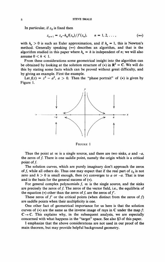
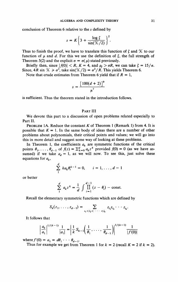
From these considerations some geometrical insight into the algorithm can be obtained by looking at the solution structure of (*) in R2 = C. We will do this by stating some facts which can be proved without great difficulty, and by giving an example. First the example.

Let f(z) = z2 - a2, a > 0. Then the "phase portrait" of (*) is given by Figure 1.

—0 ^ > , «_ x -a -̂ L ^ r &

t ^\ / \ \ K /

FIGURE 1

Thus the point at oo is a single source, and there are two sinks, a and -a, the zeros of/. There is one saddle point, namely the origin which is a critical point of/.

The solution curves, which are purely imaginary don't approach the zeros of ƒ, while all others do. Thus one may expect that if the real part of z0 is not zero and h > 0 is small enough, then (*) converges to a or -a. That is true and is the basis for the general success of (*).

For general complex polynomials ƒ, oo is the single source, and the sinks are precisely the zeros off. The zeros of the vector field, i.e., the equilibria of the equation (*) other than the zeros of/, are the zeros of ƒ .

These zeros of f or the critical points (when distinct from the zeros of ƒ) are saddle points when their multiplicity is one.

One other fact of geometrical importance for us here is that the solution curves of (*) are the same as the inverse image of rays in C under the map ƒ: C~»C. This explains why, in the subsequent analysis, we are especially concerned with what happens in the "target" space. See also §3 of this paper.

I emphasize that the above considerations are not used in our proof of the main theorem, but may provide helpful background geometry.

PART II

1. Here is a simple consequence of Theorem 1. Suppose that the polynomial

f(z) = z + a2z2+ • • • +adz

d

has no critical values f(9) in the unit disk in C (i.e., |/(0)| > 1 if ƒ'(#) = 0). Then \a2\ < 2 and it is perhaps true that \a2\ is always less than \. It is somewhat subtle even that \a2\ has any bound (independent of d).

THEOREM 1. Let f(z) = 2f»0 aiz'> a complex polynomial with a0 = 0, ax ^ 0.

Then there is a critical point 0 E C (i.e., f'(B) = 0) such that for every k = 1, 2, 3, . . .

\*k/ai\l/ik-l)\A0)\/\*i\<*.

REMARK 1. We will sometimes write instead

\ak/al\l^-»\m\/\"i\<K.

Thus K could be 4. On the other hand 4 may not be the sharpest value. I suspect one could take K = 1, but, we will give examples which show that K > 1. See also problem number 1 of Part III.

REMARK 2. The proof yields sharper results for each k. More precisely

W/ax\^-^\A9)\/\ax\ < ft where ft = 2, ft = V5 , p4 = (14)1/3, ft = (42)1/4 ~ 2.55, ft ~ 2.61, ft ~ 2.65, ft0 ~ 3.29 and of course ft < 4.

REMARK 3. The theorem is false in a quite extreme way for entire functions. There is no bound at all f or k = 2 or any k. This is even true for entire functions which have no critical points in C. For example let f(z) = (l/aje01* - l/a,a > 1.

The proof of Theorem 1 goes by a theorem of Loewner. See Hayman Jenkins, or Schober. Loewner proved this theorem at the same time that he showed that \a3\ < 3 in the Bieberbach conjecture (1923).

Define Dr to be the disk {z e C| \z\ < r} throughout.

THEOREM (LOEWNER). Let g: Dx —> C be a "schlicht" function, i.e. g(z) can be expressed as a convergent power series, g(z) = 2JL0 /̂z/> \z\ < 1> w^n

b0 = 0, bx = 1 and g is 1-1. Suppose that f: Œ —» Dx is an inverse to g with OEfl . Letf(z) = S° l 0 <*iz' near ° (therefore a0 = 0, ax = 1). Then

\ak\ <Bk, k= 1,2, . . .

where

Bh = 2 A 1 - 3 ••• (2* - 1) 1 • 2 . . . (fc + 1)

We need to extend the theorem to the case where Dx is replaced by D^ and bx T^ 0 is arbitrary.

EXTENDED LOEWNER'S THEOREM. Let g: DR ->C, (R > 0) be 1-1, g(z) =

2£.o V '» bo = °><*i ^ 0 and f: Ü-* DR be an inverse to g with 0 G Q. Let

10 STEVE SMALE

f(z) = 2 £ o ap* near 0. Then

PROOF. First let/, g be as in the extended theorem with R = 1. Note that a, ¥> 0 and in fact a, = /'(O) = 1/6, = l/g'(0). Let g0(w) = (l/6,)g(«) and U') = /(*/«.)• So

ƒ<,( &(«)) = / ( ^ ( ^ *(«))) = « for |«| < 1.

Since

/0(z) = z + 4 z 2 + 4 z 3 + • . . , af a\

and since Loewner's theorem applies to g0, we have

k/«*l < **• Thus we conclude

LEMMA 1. ƒƒ g: DX->C is 1-1, g(0) = 0, g'(0) ^ 0 a/w/ ƒ: Œ -> Z^, 0 G Œ, /(O) = 0, f(z) = axz + öf2z

2 + • • • w itó inverse, then

Next let g: D^ —> C, and ƒ be as in the extended theorem and let gx(w) = g(Rw). Then gj and fx satisfy Lemma 1 where fx(z) = (l/R)f(z), since MSiM) = (l/R)f(g(Rw)) = w. Also fx(z) = («1//J)z + (a2/R)z2 + • • • . Apply Lemma 1 to obtain

|ak / f l I |I /<*- ,>*/ | a i |<*l /<*- ,>.

This proves the theorem.

LEMMA 2. £y<*_1> < 4.

PROOF.

2 l ' 3 ' 5 ' - 2 t - 1 . ^ _ , / 2 ** " k+\' 1 • 2 • 3 • • • A: It follows.

A = 2k~l . _ ^ _ . i \ J \ J \ " ^ , x < 2 * - 1 ( - ^ - T ) 2 * - 1 < 2*"1 • 2k~\

LEMMA 3. Let f(z) be a polynomial of exact degree d,f(0) = 0 and such that

R = min \f(0)\ > 0.

A')-o 77*e« there exists an analytic function g: DR-±C with g(0) = 0, andf(g(w)) = wfor all w E DR and g is 1-1.

PROOF. First note that

/:c- u r\A9))-+c- u m 9 f'(9) = 0

is proper (the inverse image of a compact set is compact) and a local

homeomorphism. It is a covering map. Therefore we may lift it back by g over DR, uniquely if g(0) = 0. This proves Lemma 3.

Combining Lemmas 2 and 3 with the Extended Loewner Theorem yields Theorem 1.

We give some lower bounds for the constant K = Kdk of Remark 1 of Theorem 1. Thus for each k, d as in Theorem 1, let Cdk be the lower bound exhibited by f(z) = (z - 1 / - (-1)* if k < d and f(z) = zd - dz if k = d. Then

PROPOSITION. Cd>d = ((d - \)/d)(\/dy ,d-\

{d-\)\ y/<*-*>i c** \k\{d- k)\ j -i ifk<d.

COROLLARY. K OF (REMARK 1). Theorem 1 must be at least 1 (it is independent of k, d).

The proof of the Proposition is a direct calculation which we omit. Note that Q 2 = $d - $/d for all d > 2 and that CdJk < (d - \)/d for

all &, d. Note also that

1 / 1 \ 1 / 2

m a x Q 2 = - , m a x Q 3 = ^ - j ,

m , a x c - = ( V ) d ) « k>3-This gives the Corollary. We end this section by remarking that there is a large related literature on

the critical points of polynomials; see Marden.

2. Here we make some estimate on the effect of one step of our algorithm. As usual we are taking a target space perspective, i.e., estimating values. In the next section the result is used to estimate the effect of many steps.

Let K be as in Remark 1 after Theorem 1, e.g., K — 4.

THEOREM 2. Let f be a polynomial and z G C such that f(z) andf(z) are not zero. Let

h0= mm 1 m-A*) A')

and0<h < h0. Ifz' = z - hf(z)/f'(z), then

f(z')/f(z) = l - h + ah2/ (h0 - h)

for some « E C , \a\ < 1.

The proof uses the following version of Theorem 1.

THEOREM 1A. Let f be a polynomial and z G C such that f (z) ^ 0. There is

12 STEVE SMALE

a critical point 0 of f such that f or all k = 2,3,

k\f(z) \A*)-AO)\ Furthermore, iff(z) ^ 0, and h0 is as in Theorem 2, then for k = 2, 3, . . .

/*>(*) A') k-l

k\ mk

\/{k-\)

V Note first that the last statement of Theorem 1A is a consequence of the

first part. We now check the first part. For this let/, z be as in Theorem 1A and expand ƒ about z so that f(w) = 2*«0C/*(Z)/^0(w ~~ *)*• Define the polynomial g by g(w) = 5#_ !(ƒ*(*)/*!)«*. So g(w - z) = /(>v) - /(z) and g'(w — z) = /'(w). Apply Theorem 1 to g to obtain

/*(*) L/(*-l)

Thus

k\f\z)k

A*)

| g(a)| < K for some a with g'(o) = 0.

*!ƒ'(*)*

i / ( * - i )

| / ( 0 ) - / ( z ) | < # for0 = z + a.

This proves 1A. We now prove Theorem 2. Again expand ƒ by Taylor's series about z, using

z ' = z - hf(z)/f'(z\ to obtain f(z')/f(z) = 1 - h + hy where

7 - 2 (-*> k = 2

k^nz)Az)k

k\f'{z)k

Now by Theorem 1A we obtain

M< 2 k = 2

Thus

|y|< 2 / « I

= 2 / = 0

1 < 1 - h/h0 h0- h

Let a = ((*o - A)/A)y; then |<x| < |y| \(h0 - h)/h\ < 1. This proves Theorem 2. We apply Theorem 2 to obtain information about Newton's method.

COROLLARY A. Let C > \ and pj — p = min^^w.0 |/(ö)| for a polynomial j \ If Iƒ(*)! < P/CK + K + 1 then \ f(z')/f(z)\ < \/C where z' - z - f(z)/f\z) {Newton's method).

PROOF OF COROLLARY A. We first remark that for any critical point 0, \f(0) - f(z)\ + |f{z)\ > |/(0)| and \f{9) - f(z)\ > \f(9)\ - \f(z)\ > p -|/(z)|. By hypothesis, \f(z)\(CK + K + 1)< p, so | /(z)| tf(l + C ) < p -

\f(z)\. Thus by the prior remark, for any critical point 9, \f(z)\K(l + C) < \f(0)-f(z)l

Thus we have shown that for any critical point 0,

\f(9)-f(z)\/K\f(z)\>l + C.

So for h0 of Theorem 2, we have h0 > 1 + C and l/(h0 — 1) < 1/C. Apply Theorem 2 with /* = 1 to obtain

\f(z')/f(z)\< l/(h0-l)<l/C.

This proves Corollary A.

COROLLARY B. Let K and p be as before with \f(z)\ < p/(2K + 1). Then Newton's method starting at z converges to z*, a solution off(z*) = 0. (Recall we could take K = 4.)

PROOF. Choose C > 1 such that \f(z)\ < p/(CK + K + 1). Use Corollary A. If z, = z - / (z ) / / (z ) , then \fizx)/f(z)\ < 1/C. Inductively let z„+1 = zn

- f(zn)/f'(zn). Thus |/(zrt+1)| < (l/C)|/(z„)| < p/(2K + 1), so f\zn) is never zero and \f(zn+l)/f(z)\ < (1/C)rt+1. This proves Corollary B.

Note that Corollaries A and B give a new criterion for Newton's method to work. This is used strongly in our main result.

3. Here we make estimates in the target space or on the values /(z0),/(z^, /(z2), . . . as the algorithm constructs zv z2 , . . . . Under suitable initial conditions, it must be shown that f(zn) tends to zero sufficiently faster than it veers off toward some critical value f(9). At the critical points, the algorithm is not defined, and near them goes very slowly. Thus this analysis is central. We use heavily Theorem 2 of the preceding section.

Throughout K will be the constant in the remark after Theorem 1. Certainly K > 1 and K could be taken as 4. As in §2, pf is the number

pf= min |/(0)|.

We now define for each polynomial ƒ and z0 e C such that f(z0) ^ 0 and P / > 0 ,

3C = jCtr — min * ° o

\/(0)\<2\f(zo)\ {••KM

Moreover, under the same conditions, define

(3tf+l) | / (2 0 ) |

THEOREM 3. There exist two universal functions H: R+ X R + - » R + , S: R+ XR + —»Z + , exhibited later, with these properties: If f, z0 satisfy pj > 0, % = %Uo > 0 and h = H{%, ?), * = S(%, f) then zk = zk_x -hf(zk_l)/f'(zk_1) is well defined inductively for all k starting from k = 1 and

14 STEVE SMALE

| f(zs)\ < py/(3K + 1). Moreover H and S have the form

1 sin2(3C/2) H(%, f ) = # (3 sin(3C/2) + logf)

S(%, f ) = */a |3 + *«** V 1 sin(9C/2)/

REMARK. According to Corollary A of Theorem 2, for k > s, one can change h to 1 (Newton's method) so that zk —> z* as k —> oo with /(z*) = 0. After s steps, we have found an approximate solution.

Define h^ = (l/K) sin(3C/2). The following is the main lemma.

LEMMA 1. Suppose s G Z + , 0 <h < h+/2, depending on f, % of Theorem 3 satisfy (1) and (2).

( I - A + A 7 ( A , - A ) ) ' < 1 / £ ,

4,)(T^) < sin-%

(1)

(2)

77ien the conclusions of Theorem 3 {except the last sentence) are satisfied with these choices of h and s.

Note that once Lemma 1 has been proven, the rest of the proof of Theorem 3 amounts to solving equations (1) and (2) for h, s and exhibiting their dependence on % and f.

For the proof of Lemma 1, we use

LEMMA 2. (a) For any r, £ G C, (3 ¥> 0, |sin arg((/? + r)//3)\ < |r/j8|, (b) |sin arg(/(0)//(z))| < |(/(z) - f(9))/f(z)\ if f{z) * 0, (c) for 0<h< hjly a G C, |a| < 1,

sin arg 1 — h + K - A ) N A , - A ) ( I - A ) -

PROOF OF LEMMA 2. (a) can be checked via trigonometry, (b) follows from (a) with T = ƒ(#) - /(z), £ = /(z). For (c), take in (a), 0 = 1 - A, r = ah2/(h* - h).

LEMMA FROM TRIGONOMETRY.

|sin 2 a/| < 2 lsin ai\-

Let z0 be given as in Theorem 3. We proceed by induction to prove Lemma 1. Let k < s and suppose inductively for / < k that f'(zt) ¥= 0, and hence z/+i = zi ~ hf(zi)/f'(zi) is well defined, and moreover

ht = — mm K 9

f'(0) = 0 A*i)

>h±.

Note that if ever f(zk) (or /(z,), i < k) is zero, we are finished trivially. To

finish the induction, we will show that f'(zk) ^ 0 and hk > h^.

LEMMA 3.

k A'*) fUo) h+&) < i ,

arg A'k) fro)

< %

(a)

(b)

PROOF OF LEMMA 3. First write f(zk)/Kz0) = f(zk)/J(zk_{) • • • foù/A^o)-So we may apply Theorem 2 to obtain

a,h2 A',)

= 1 - h + hi-x-h

i=\,...,k,\ai\<\,0<h< h,_ A*,-i)

By the induction hypothesis ht_x> h^, i = 1, . . . , k, and thus since h < h^/2, we have

1 - h + a,h2

Therefore

h,-x ~ h

M)

< 1 -h +

This proves (a) of Lemma 3. For part (b) we have

1 - h + h,- h

A'k) 4 ( A',) \

and thus by the lemma from trigonometry,

sin arg-_A'k) 'A* J

But by Lemma 2(c) we may estimate

< 2, sin a r g - -

sin arg A*,-i) \hi_l-h]\i-h)< [h.-h)(i-hy

thus

sin arg _A*k) A*J <^)(rh>

By (2), since k < s,

sin arg _M) A'o)

< s i n T < T ,

the last since |arg(/(zÂ:)//(z0))| < % < 1. This proves Lemma 3.

16 STEVE SMALE

Now |arg(/(0)//(zo))| > % for any critical point 9 e C such that | f{9)\ < 2|/(z0)|. Since

'ƒ(*„) 'M) arg ƒ(*<>) '

we conclude from Lemma 3 that |arg{/(0)//(zt)}| > %/2 for any critical point 9 with \f(9)\ < 2|/(z0)|. In particular, \f{zk)\ < 2|/(zo)| (Lemma 3(a)) so that zfc is not a critical point, ƒX^) ¥= 0.

Next, |sin arg(/(0)//(z*))| > sin(3C/2), so using Lemma 2(b)

A'k)-M) ƒ(**)

sin arg > s i n T

for any critical point 0 such that | /(0)| < 2|/(z0)|. On the other hand, if |/(0)| > 2|/(z0)|, since \f(zk)\ < |/(z0)|,

A*k)-m A**)

> 1 > sin %

Therefore

hk = min 1 A**)-A0)

ƒ(**) > — sin y = /i#.

f'(0) = 0

This finishes the induction. To finish the proof of Lemma 1, one has to show that \f(zs)\ < pf/(3K + 1). Use Lemma 3(a) to get \f(zs)\ < (1 - h + * 7 ( * , ~ h)y\A**>V So IM)I < 0 / 0 1 /(*o)l by (1) which in turn is less than Pf/(3K + 1) by the definition of f. This proves Lemma 1.

Now we solve (1) and (2) for h and s to finish the proof of Theorem 3. Recall

('-•^)<f

(1) is equivalent to

log f

and (2) to

l o g ( l - h + h2/(hm-h))~

\ (1 - A)(A, - h) s <Khm

<s

(1)

(2)

(1')

(2')

LEMMA 4 (EASY). log(l/(l - y))>y ifO <y < 1.

In (1') let y = h - h2/(/»„ - h) = /*((/*„ - 2A)/(A» - A)) and use Lemma

4 to see that (1") implies (1').

^ < 3 . (1") y

Next use h = h^/C where C > 2 to replace (1") and (2') respectively by

s <K(C - h*)(C- 1). (2")

Besides (1'") and (2"), we have the condition that s be an integer.

TECHNICAL LEMMA. If C > 3 + log Ç/Khm, then

( l o g n ^ ( § ^ l ) + K*(c:- *,)(c- i).

PROOF OF TECHNICAL LEMMA. Note first that if C > 3 then

C - 2 1 / 1 „ , \ t

(using /**<! , since 3C < 1).

Therefore from the hypothesis of the Technical Lemma,

log? ( C - 2 ) Khm + ^ ( 0 c V » . ) «

Next divide and multiply through this expression to obtain the Technical Lemma.

To finish we choose C = 3 + log f /Khm and h = h+/C. Then choose s to be the greatest integer in (log f )(C//**)((C - 1)/(C - 2)) + 1.

In fact we may calculate h and s more explicitly as follows.

h = Kh\l (log f + 3/^tf), h+ = (1/ /Q sin2(3C/2)

giving H(%9 f ) as in Theorem 3. Going back to (2") we could take s as simply KC2 since increased 5 (fixed

h) will still satisfy our conditions in Theorem 3. Then

___ / ( l / i Q s i n ( 3 C / 2 ) \ 2 _ ir(3sin(3C/2) + logf)2 _ / ( l / i Q s i n ( 3 C / 2 ) \ 2 _

sin2(X/2)

This finishes the proof of Theorem 3.

4. This section gives the main probability (or volume) estimates which are used in our statistics. Our approach is more geometric than measure-theoretic although we do make use of Fubini's theorem. There is an interesting historical point about a theorem of Herman Weyl on the volume of tubes that we use. The statistician (and economist) Harold Hotelling proved a result on the volume of a tubular neighborhood of curves (see Lemma 2 below). This is motivated by problems of regression equations in theoretical statistics. Subsequently Hotelling9s theorem was extended by Weyl (see Lemma 5 below) and

18 STEVE SMALE

these two papers lie next to each other in the American Journal of 1939. Weyl writes: "In a lecture before the Mathematics Club at Princeton last year Professor Hotelling stated the following geometric problem as one of primary important for certain statistical investigations: . . . ." and Weyl goes on to state and prove his theorem on the volume of tubes.

In the intervening years Weyl's result has become well known to geometers; see Griffith's extensive discussion. Now the result of Weyl is found useful in our statistical analysis.

There is another amusing aside in this connection. In the use of Weyl's theorem, I had need to estimate the integral of the Gaussian curvature A" of a complex algebraic curve y in C2 in terms of the degree 8. I took this problem to Osserman and after a little thought, using his joint paper with Hoffman he came up with the neat estimate:

±fK<-S(S-l).

This is nice because the volume of y is infinite, and it might also have singularities where the curvature blows up. Although I believe this estimate is not explicit in the literature, it now follows easily from standard results. Griffiths subsequently showed me another proof.

Eventually, I bypassed the need for the estimate by noticing a simple sign argument which did the trick.

We proceed to the theorems on volume estimates. Let 9d be the space of polynomials of degree d with leading coefficient 1. Thus 9d can be identified with complex Cartesian space C* = {(a0, . . . , ad_x) = a\at G C} or we may write ƒ G Cd where/(z) = Sf«0

atz^ ad = *• L e t P(R) denote the polycylin-der {a G 9d\ \at\ < R, i = 0, . . . , d - 1}. Note that the volume of P(R) or vol P(R) is (vrR2)d. Here we use the standard volume on C* - R2d for 9d.

Let ^ 0 = { / 6 9d\K0) = 0 for some 0 with ƒ'(#) = 0}. It is easily seen that W0 is the set of ƒ with multiple roots. Finally define Up(W0) = U / e ^ 0 VpUo) where Up(f0) = {ƒ G %\ \f(0) - /0(0)| 0, coincide.

THEOREM 4A.

VQI[UP(W0) n P(R)] dp2

Vo\P(R) < jR2 *

This theorem is not used in the sequel; however it serves as a simple prototype of Theorems 4B and 4C which are important for our development.

The proof of Theorem 4A goes via

PROPOSITION 1. The subset W0 c 9d a Of has a representation as a complex algebraic hypersurface given by a single polynomial equation of degree 2d — 1 which is of degree d in a0. More precisely, there is a polynomial F: C? —> C,

d

F(a0, . . . , ad_x) = 2 Ft(a\, • • • , a</-iK, i -O

where the Ft are polynomials, F has total degree 2d — 1 and

W0= {aSCd\F(a)=-0}.

PROOF OF PROPOSITION 1. Note that

W0 = { ƒ G %\ f(9) - 0, ƒ'(0) - 0 for some 9 e C}.

Then the proof goes by the description of the resultant (see Van der Waerden, Vol. I (p. 84) or Lang). Thus F is the resultant of ƒ and ƒ', R(f,f). The proof of the proposition then follows from an examination of the form of R(ƒ, ƒ') given in either reference.

For the proof of Theorem 4A, define x: C -> R to be the characteristic function of Up( W0)9 i.e., x is 1 on Up( W0) c C and zero off of it.

Now observe that for almost every (in the sense of Lebesgue measure) (a„ . . . , ad_x\ W0 intersected with the one (complex)"dimensional coordinate plane through (a„ . . . , ad_x) consists of at most d points. This follows from the proposition, with the exceptional (ax, . . . , ad_x) being those points where all the Fi vanish. From this, using the definitions, we may conclude that for almost every (a,, . . . , ad_x)9

f x(a0>- • • >ad-i)dao JWo\<R ;

< driTp2

Thus by Fubini's theorem

Vol U(W0) n P(R) 1 ƒ X(a)

Vol P(R) {vRiy-'PW

1

da

( r f 2 r i« i i<« f ( Xi.a0,...,ad_x) dar,

>ol<* dax • • • dad_x

k,-il<*

< — - — f (dirp2) dax

{TTR2)dJ\aA<R,>..,\*d-i\<R

< _L^ (^p2 ) My-i < V >2\d R2

dad-i

This proves Theorem 4A. We will now use Re z and lm z systematically for the real and imaginary

parts of a complex number z. Consider the subspace W* of <$d9 W* = {ƒ G 9 d\lm(j(G)f(9)) = 0 for

some critical point 9 of ƒ}. So ƒ E J ^ provided Re/ ' , I m / and Im(/(0)/) have a common zero. Let Up(W+) = UfoGW Up(f0)9 where Up(f0) is defined earlier in this section.

20 STEVE SMALE

THEOREM 4B.

Voi[e/p(y,)n/>(*)] <3P(d-i)2

Vol P(R) < R

The proof of this theorem uses the following Algebraic Lemma.

ALGEBRAIC LEMMA. The set W+ c 9d is a closed subset of a real algebraic variety in R2d — C*. In fact this variety is the set of zeros of a real polynomial G in the 2d variables (Re ai9 Im a,-)f ~o and G has degree (d — l)2 in (Re a0, Im a0).

To prove the Algebraic Lemm$, we use elimination theory which can be found in Van der Waerden, Vol. II. See especially p. 15.

THEOREM FROM ELIMINATION THEORY, n generic homogeneous polynomials in n-variables have a resultant F which is an integral polynomial in their {indeterminate) coefficients. The vanishing of this resultant for particular j \ 9 . . . , ƒ„ with coefficients in a field is a necessary and sufficient condition for the existence of a solution (perhaps in an extension field) of the system of equations fx = 0, . . . ,fn = 0, distinct from the zero solution. The resultant is homogeneous in the coefficients of fk of degree Dk = 11,^ dt {the product) where degree

f, = 4-We need to apply this result to the case of n inhomogeneous polynomials in

(n — 1) variables. This is done as usual by adding a new variable to homogenize the polynomials. New solutions may be introduced, however. We obtain in this way

COROLLARY. Let %9 i = 1, . . . , w, be given spaces of inhomogeneous polynomials f of degree dt in (n — 1) variables over a fixed field K. Thus % can be identified with the space of coefficients of f. Then there is a polynomial (the resultant) F: JTJ„ x ^ —> K in the coefficients of these f with the property that if particular j \ 9 . . . ,fn have a common zero, then F(fl9 . . . ,ƒ„) = 0. Furthermore F is homogeneous in the coefficients of f of degree Dk = Wiwm\.yi=fLk dt.

Now fix the field to be R, the real number field. Let ^ and % e a c n ^ e t n e

space of real (inhomogeneous) polynomials of 2 variables of degree d — 1. Let % be the space of real polynomials of 2 variables of degree d.

The above corollary applies to yield a polynomial F: f , x f 2 x f 3 - 4 R such that F(gv g2, g3) = 0 whenever gv g2, g3 have a common zero (x9y) e R2.

Next define a map O: <$d -> % X % X % $ = (pl9 02, 0>3) by $(ƒ) = (Re/ ' , I m / , lm(f(0)f)). Here ƒ', the derivative of/, may be naturally interpreted as the sum of 2 polynomials, ƒ ' = Re ƒ' + i Im ƒ , where Re ƒ is a real polynomial of 2 real variables (C = R2) of degree d — 1. Similarly Im(/(0)/) has a natural interpretation as a real polynomial of 2 real variables of degree d. Explicitly Im f(0)f is the imaginary part of the polynomial

d

S («o+ iPo)(«k + #k)(x + M* A; = 0

where ak = ak + ipk, k = 0, . . . , d and i = V^T (recall ad = 1). Thus $ is well defined and moreover $x ƒ, $ 2 / are independent of a0, /?0

and $ 3 is linear in a0, y80. From the construction of F: % X % X ^ -^ R, if ƒ E W^, then F o <!>(ƒ)

= 0. Let G = F ° $ . Then G is a polynomial in the a0, /30, . . . , c^-j , &_, which has degree (<tf - l)2 in (a0, /?0). This finishes the proof of the Algebraic Lemma.

Now let y be a plane real algebraic curve of degree 8. Thus y can be thought of as a locus of zeros in R2 of a real polynomial F(x9 y) of degree 8 (8 = (d — l)2 in our application). The singular points of 7 are those points in R2 which are common zeros of dF/dx and dF/dy. Thus by Bezout's theorem there are at most (8 — l)2 singular points.

Let N (y) be the set of all points in R2 within p of some point of y. Let DR c R be the open disk of radius R > 0 about zero.

PROPOSITION 2. If y is a real plane algebraic curve of degree 8, then

area[7Vp(y) n DR] < 3nR8p.

For the proof introduce the set Tp(y) c R2 of all points which lie on line segments of length z a singular point of y.

Here Dp(z) is the disk of radius p about z.

For the proof of Lemma 1, let x G Np(y), x G DR. Then there is y E. y such that d(x,y) < p and we may suppose d(x,y) is minimal. Therefore y E DR+p. If y is a singular point, then x E Dp(y) c V . If y is not singular, tnen since d(x, y) is minimal, x lies on a normal segment to y at y of length less than p, i.e., x E !Tp(y n DR+P)- This proves Lemma 1.

The following is a special case of a theorem of Hotelling.

LEMMA 2. Let y0 be a smooth plane curve with nonvanishing tangent {but not necessarily connected) of total length I. Then

Area rp(y0) < 2p/.

LEMMA 3. Let y be a real algebraic plane curve of degree 8. Then the length Ky H DR) is given by

l(y n DR) < 7T&R.

For the proof of Lemma 3, we follow Santalo pp. 17-31 and especially pp. 30-31. Let dG be the standard measure on the space of lines in the plane. The

22 STEVE SMALE

length L of a curve C satisfies(5'a«/a/ö p. 31)

2L = ƒ « dG

where « is the number of points of intersection of a line and the curve. The integral is over all lines. Now in our case, almost every line (in the sense of our measure on the space of lines in R2) meets C in at most 8 points. This is a very special case of Bezout's theorem. Moreover, the integral is just over the lines which meet DR. So

2L <ôf dG <8 ITTR. •'lines meeting DR

The last evaluation, that

dG = 2<rrR, L lines meeting DR

is shown on Santalo p. 30. This proves Lemma 3. We now give the proof of Proposition 2. Use Lemma 1 to obtain

Area(7Vp(y) n DR) < Area Vp + Area Tp{y n DR+p).

Clearly, Area Vp < 7rp2(8 — l)2 since there are at most (8 — l)2 singularities (again we use Bezout's theorem). By Lemma 2, Area Tp(y n DR+P) < 2p/(y n DR+p) and by Lemma 3, this is less than 2pir8(R + 8). Putting these estimates together yields

Area(7Vp(y) n DR) < irp2(8 - l)2 + 2p(9w(R + p))

<7r[2p8R +p 2 [2ô + ( ô - l)2]]

<7r[2p8R + p2(ô + 1)].

Now observe that if p > R/38, then 37r8Rp > TTR2 and since

area[A^p(y) n DR] < area DR < TTR2,

the proposition is true in this case. Thus for the proof we may assume p < R/38. Since (Rp/38)(82 + 1) <

8Rp (easily checked), p2(82 + 1) < 8Rp. Together with our previous estimate this yields the proposition.

Now the proof of Theorem 4B proceeds as the proof of Theorem 1A. Let X: C* « R2</—»R be the characteristic function of Up(W+). Now represent W+ as in the algebraic lemma. The almost everywhere considerations used in the proof of Theorem 4A apply here as well. Thus by Proposition 2, for almost every (av . . . , ad_l%

J\*o\<R < 3(d - \yirpR

Then by Fubini's theorem,

Voiu,(wm)nP(R) i r r , Vnl P(R\ = ^ I , i X ^ ° ' ' ' • ' a*-V daSda\ • • • dad-\

\<*d-i\<R

< 3(d- \firpR( da {<nR2)d •V1|<*,...,k,_1|<*

I - ^ - 1

This proves Theorem 4B. Define

ff, = { / 6 ®d\A0) = A°) f o r s o m e critical point 9).

Let

M/o) = { / ^ l / ' ( 0 ) - / o ( 0 ) | < p a n d f"(0) # ( 0 ) 2 2 < P

and

Lp(Wx)~ U L P U ) , / 0 e W,.

THEOREM 4C.

M^ (FF,) n P(R)] (£_, \2(d + D.

VolP(#) V # / v

As in the proof of Theorem 4A we use the resultant to describe Wx as a variety in C1. The basic fact is that ƒ G Wx if and only if ƒ and ƒ — /(O) have a common zero. As in van der Waerdan, Vol. I, and Lang, we consider the resultant R(f\ ƒ — /(O)) as a polynomial F in the coefficients (a0, ax, . . . , #</_!). Note here that of course ad = 1, and also that F is independent of a0. Furthermore it can be seen from the form of the resultant that F has degree (d + 2) in (ax, a2).

On C2 we will use the norm || \\B, defined by \\z\\B = ||(z„ z2)||^ = max(|z,|, |z2|).

PROPOSITION 3. Let y be a complex algebraic plane curve of degree 8 > 3 and define

Np(y) = {z G C2| \\z-y\\B (*)] < 4Ô(7rpR)2.

24 STEVE SMALE

Here P(R) is the polycylinder DR X DR9 DR the disk of radius R in C. The proof of Proposition 3 is analogous to the proof of Proposition 2 with

Lemmas 4, 5, 6 playing the role of Lemmas 1, 2, 3 respectively. Also Proposition 3 plays the same role in the proof of Theorem 4C that Proposition 2 did in the proof of Theorem 4B.

Define Tp(y) just as in Lemma 1, in terms of distance along line segments normal to the surface y in R4. The same applies to Tp(y n P(R + p)). Define

v„ - U PÀP)

where 2 is the set of singular points of y and Pz(p) is the polycylinder

PZ{P) = {y e C2| \\y - z\\B < p).

LEMMA 4.

Np(y) nP(R)aVpu Tp(y n P(R + P)).

REMARK. It seems likely that this is true omitting Vp. However, this doesn't affect our estimates much and we leave it in. P. Griffiths, in conversation, has confirmed the possibility of omitting V .

PROOF OF LEMMA 4. Let x e P(R) n Np(y). Suppose y e y minimizes II* ~ y\\B- Thus ||x — y\\B > E P(i? + p). This proves Lemma 4. See Weyl (1939) (and also Griffiths) for the following

LEMMA 5 (WEYL).

Vol Tp(y) < 7T Tarea^ê// Here y is supposed to be a smooth surface in R2 with equality in the case of

no overlapping. Actually Weyl supposes y is compact, no boundary (or singularities). But his analysis applies to our situation as long as we interpret Tp via normal segments. In the integral K is the Gaussian curvature of y.

We first note that since y is a complex algebraic curve, it is a minimal surface; therefore everywhere K < 0 and we may discard this term. See also the introduction to this section.

LEMMA 6. If y is a complex plane algebraic curve of degree 8, then

area[y n P(R)] < 6<JT8R2.

PROOF OF LEMMA 6. Here we follow Santalo once more. We integrate functions over the space of 2 dimensional planes in R4 = C2.

This goes as follows. We write L2 for a typical 2-plane in R4 and dL2 for the measure over the space of such planes. Then

- ^ area(y n P(R)) < ƒ # ( y H L2) dL2

where # (y n L2) is the number of points of intersection of y and L2 (see

Santalo, 14.70, p. 245). Here Ok is the surface area of the unit fc-sphere and in particular O0 = 2, Ox = 2TT, 02 = 4TT, 02/04 = 3/2TT (Santalo, p. 9).

Now # ( y n L2) < 8 by Bezoufs theorem except for a set of L2 of measure zero. Then

f # ( y n L2)</L2 < ô f </L2 ^ 2 JL2nP(R)¥-0

Now for any convex set # (Santalo, p. 233), SLinKdL2 is evaluated in terms of a certain quermassintegrale Wr(K), Thus

ƒ dL^l-^-W^K)-

I was not able to use Santalo's formula (p. 225) for K = P(R)\ so crudely use the fact that P(R) C DV2*, the ball, and Santalo9s evaluation on p. 224

* W V 2 * ) = 03R

2

2

Thus

ƒ Oi02 -

Putting these estimates together we obtain

°2°\ * °3 area(y n P(R)) < -7r7r8TT°2R2 < 6 ^ 2 .

This proves Lemma 6. We now are able to prove Proposition 3 in much the manner of Proposition

2. First use Lemma 4.

Voi(tfp(Y) n P(R)) < vol vp + Vol rp(y n P(R + P)), where

Vol F p < (Ô - l ) 2 Vol P(p) = (Ô - 1)2(TTP2)2 .

By Lemma 5 (and comments), 2

Vol Tp(y n P(R + p)) < w^- area(y n P ( * + p));

then using Lemma 6, 2

Vol r p ( y n i>(* + P» < ^ J - 6ir8(tf + p)2,

so Vol[ JVp(y) n /»(*)] < »rV(* " O2 + f T2P2«(* + p)2- (*)

Now we prove the estimate of Proposition 3 in two cases. First suppose that

26 STEVE SMALE

p > (2/38)l/2R. Then

48ir2R2p2 > (TTR2)2 > Vol P(R) > Vol[Nfi(y) n P(R)].

On the other hand, suppose p < (2/3ô)1/2R. Use our previous estimate (*). So we have to show that if p < (2/38)l/2R9 then

<rr2p4(8 - 1)2+1<IT2P2Ô(R + p)2 < 48ir2p2R2

p2(8- \)2+l8(R + p)2 <48R2

or

or yet

2

382 (,-tf+»(,+(â)7<* But this last is easily checked using the fact that 8 > 4. This proves Proposition 3.

It remains to prove Theorem 4C, which will follow closely the proof of Theorem 4B. Thus let x- C* -» R be the characteristic function of Lp(Wx).

Now we have shown that Wx is a complex hypersurface in Cr with the property that for almost every (a0, a3, a4, . . . , ad_ x\ it has degree (d + 2) in ax, a2- Furthermore

LP(W\) = U {(a0, a'v a'i> Ö3, . . . , ad_l)\

X \a\ - ax\ < p, \a2 - a2\ < p}, (a0, ax, . . . , ad_x) G Wv

By Proposition 3, for almost every (a0, a3, . . . , ad_ x)

[ XK> • • • > flj-i) ^ 1 ^ 2 < 4(rf + 2)(7rpi?)2.

Then

Vol L p ( ^ ) n />(*) VolP(tf)

< Z ^ 1 0 K . f/x(^..-.^.)*.^ v ' l«3|<*

ö^n da.

k#-il<*

2\d M2) I |«bl<*

k#- i l<*

da0da3 .da. 4{d + 2){vpR)2

or

Vol/W M y 2

' * 2

This proves Theorem 4c.

5. Here we will prove our main result, as stated in the introduction and in Theorem 6. Toward this end we combine Theorem 3 and Theorems 4B, 4C. This is done by first using Theorems 4B and 4C to prove Theorem 5. Then the main result will follow easily from Theorems 3 and 5.

We take UaR(W+) as defined in §4 and define

Qa = {ƒ G %\ \f(0) - f(0)\ < a for some critical point 0},

n - a u uaR(w,y THEOREM 5. (\)IfR > j ,

(2) Let o < 1 and ƒ g Ya. Then (a) P / > oR, (b) 4i* sin 3Ç > a2.

Here (see also §3)

Pf = mm |/(0)|, % = 3Ç = min l a r g ^ i

For the proof of (1) we use Lemma 1.

LEMMA 1. If o < | , Qa n />(#) c La(Wx\

a = max{2a2/3,a1/3,6/?a1/3}

w/iere La( P^) is defined in Theorem 4C.

PROOF. Let f e Qa n P(R), f(z) = 2?_0 <%*'> A») - /(0) - *, |* | < *,

ƒ'(#) = 0. We will construct f0 G ^ such that ƒ G La(/0). There are two cases to consider; first suppose that |0| > a1/3. Define in this case f0(z) = f(z) — cxz — c2z

2 where cx = 2b/'0, c2 = -b/02. One can compute directly that \cx\ < a, \c2\ < a, so that it remains to show f0 G Wv To do that it is sufficient to prove that /ó(0) = 0 and f0(0) = /0(0). But both of these are checked by direct calculations.

To finish the proof of Lemma 1, it remains to construct the desired fQ in case |0| < a1/3. For that let f0(z) = f(z) - axz and choose 0' - 0. Then clearly ^(0 ' ) - 0 and /o(0') - /0(0), so f0 G Wv To show ƒ G La(/0), it is sufficient to prove that \ax\ < 6Rol/3.

28 STEVE SMALE

Since ƒ'(#) = 0, 2 l _ 0 kakOk-1 = 0, so

N 2 K *̂'1 * » 2

The last uses the fact that \ak\ <R since ƒ G ƒ>(/*)• Thus

\ax\ < * f ^(a1/3)*-1 < * ( f ^(a1/3)*-1 - l ] A: = 2 I A:-0 J

But f or 0 < p < 1

We conclude for ft = a1/3

H <i* 1

(1 - Pf 1 } <R m - i8)

(i - Pf Now

Thus

— ^ r < 6 iI0<\oTo<j. (1 - Pf 2 8

1̂ 1 < R6p = 6Rol/\

This finishes the proof of Lemma 1. The proof of (1) of Theorem 5 now goes as follows. We may assume a < | .

Use Lemma 1 with a = 6Rol/3 taking into account the limitations R > } , a < | . First

Voi(yCT n P(R)) V o l ( M ^ * ) n P(R)) vol(Qa n P(R)) Vol P(R)

By Theorem 4B,

Vol P(R) Vol P(R)

Vol(UaR(wJnP(R)) — < 3o(d - 1) .

Vol P(R)

By Lemma 1 and Theorem 4C,

Voi(eCT n P(R)) ^ Voi{LeRMwx) n />(*)) < 144(rf + 2)a2/3.

VolP(i?) Vol/>(/*)

We may now suppose that I50(d + 2)4/3a2/3 < 1. This implies af2a < (1/150)3 < 23/2 so that 3a(d - l)2 < 6(</ + 2)4/3a2/3. On the other hand

I44(d + 2)a2/3 < I44(d + 2 ) 4 / V / 3 ;

thus

3a(rf - l)2 + 144(rf + 2)a2/3 < I50(d + 2)4/3a2/3.

With our previous estimates, this proves (1) of Theorem 5.

LEMMA 2. ƒ E Up(WQ) if and only if pf < p (here Up(W0) is defined in §4).

PROOF OF LEMMA 2. We have to show ƒ E Up(W0) if and only if |/(0)| < p for some critical point 9. By definition, ƒ E Up(W0) implies there is some f0 E W0 with ƒ E Up(f0). Thus |/(z) - f0(z)\ < p for all z. But there is some critical point 9 with /o(0) = 0 since f0 E W0. Also ƒ and / 0 have the same critical points. Thus ƒ E C/p(WT0) implies |/(0)| < p some critical point 9. Conversely if |/(0)| < p for some critical point 0, define f0(z) = f(z) — f(9). Then f0 E W0 and ƒ E Up(f0). This proves Lemma 2.

Since W0 c W„ t /p(^0) C Up(WJ and ^ ( ^ 0 ) C ^ ( ^ * ) . This yields (2)(a) in Theorem 5.

Incidentally (not used here), we have as a Corollary (use Theorem 4A),

PROPOSITION.

V o i { / 6 g j P / (i?) < /?2 '

For the proof of part (2)(b) of Theorem 5, suppose that f & Qa. We will show that under the estimate 4R sin %f <o2,f E UaR(W^).

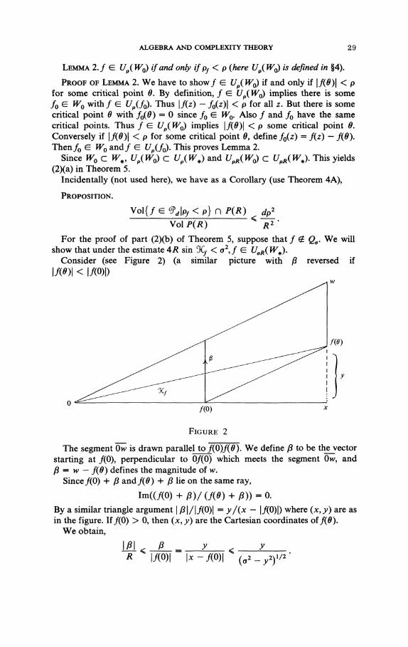
Consider (see Figure 2) (a similar picture with P reversed if l/WI < l/(0)|)

FIGURE 2

The segment (hv is drawn parallel to /(0)/(fl). We define /3 to be the vector starting at /(O), perpendicular to 0/(0) which meets the segment 0H>, and P = w — f(9) defines the magnitude of w.

Since/(0) + ft and f(9) + /? lie on the same ray,

Im((/(0) + / ? ) / (ƒ(*) + 0 ) ) - O . By a similar triangle argument | /3|/|/(0)| = y/(x — |/(0)|) where (x,y) are as in the figure. If /(O) > 0, then (x, j>) are the Cartesian coordinates of f(9).

We obtain,

I I I * " 1/(0)1 k - /(0)| ^ {a2_y2y/2-

30 STEVE SMALE

The last inequality is true since \f(9) - f(0)\ > o (f & Qa) and thus

\x - f(0)\2 + y2 > o2.

So\x-f(Q)\>(o2-y2)1/2. Furthermore

LEMMA 3.

— y - — < « . (a2 - y2)1/2

PROOF OF LEMMA 3. By multiplying and squaring the inequality becomes

y2 < a2(o2 - y2) or y2{\ + a2) < a4

or yet^ < a2 / ( l 4- a2)1/2. Since a < 1, \o2 < a2 / ( l + a2)1/2 and it is sufficient to prove that

2y < a2.

Nowj> = x sin %f9 x < \f(0)\ < 2R, so by our hypothesis 2y = 2x sin 3Ç < 2|/(0)|sin 3Ç < 4R sin SÇ < a2. This proves Lemma 3.

Now by Lemma 3 and the preceding inequality we have

^ • < a or | j 8 | < o * .

Letf0(z) = f(z) + p. Then f0 E WJ E */,„( W,) C UoR(Wx). This finishes the proof of Theorem 5.

THEOREM 6. Suppose 0 < JU, < 1, */ are g/ue« a«J i? > \. Let a be chosen so that Vol(7CT n P(R))/ Vol P(R) <fi and let f E P(#) witó ƒ « yo. 7fe/i for a suitable choice of h depending on (/A, d), and z0 = 0, zk = zk_x — hf(zk_l)/f'(zk_l) is well defined for all k and zs is an approximate zero of f where

-A log(15/q)8/n2 n _ / M 3 / 2 _ L _

Thus an approximate zero is obtained after s steps with probability of at least 1 - /A.

Define a( //,) by

a ( M ) = ( ï f e ) 3 / V ^ -Therefore by Theorem 5(1),

Vo i ( y o 0 i ) n iW) <ix

Vol P(R)

for all ju, 0 <[i < 1. This construction complements the second sentence of Theorem 6. Now for the proof, suppose ƒ £ 7 0 , / G P(R). By Theorem 5(2), %p

pf > 0, so Theorem 3 applies. In fact we obtain for a suitable A, the

conclusion of Theorem 6 relative to the s defined by

-<[ 3 + _Jog£_)a

sin(3C/2) J

Thus to finish the proof, we have to translate this function of f and % to our function of JU, and d. For this we use the definition of f, the full strength of Theorem 5(2) and the explicit a = a( JU) stated previously.

Briefly then, since |/(0)| < R, K = 4, and pf > oR, we can take ? = 15/a. Since, 4R sin % > a2, take sin(3C/2) = a2/R. This yields Theorem 6.

Note that crude estimates from Theorem 6 yield that if R = 1,

[100(</+2)]9

is sufficient. Thus the theorem stated in the introduction follows.

• " • /

PART III

We devote this part to a discussion of open problems related especially to Part II.

PROBLEM 1 A. Reduce the constant K of Theorem 1 (Remark 1) from 4. It is possible that K = 1. In the same body of ideas there are a number of other problems about polynomials, their critical points and values; we will go into this in more detail and suggest some way of looking at these problems.

In Theorem 1, the coefficients ak are symmetric functions of the critical points 0i, . . . , 0d_l of f(z) = 2^«o akzk provided /(O) = 0 (as we have assumed) if we take ad — 1, as we will now. To see this, just solve these equations for aki

d

2 kak0?-1 = 0 , / = 1, . . . , < / - 1

or better

i -d-?,akz

k = ± f I I (* - 0t) - const. 1 a J / = 1 1

Recall the elementary symmetric functions which are defined by

Sk(zv ...,zd_l)= 2 V'2* • • zk' i\<h< • • ' <k

It follows that

i i / ( * - i ) 1 * 5 * - V i " ' " 0,_J

. ! / (*-!) j

1/(0)1 where /'(O) = ax = d0x • • • 0d_v

Thus for example we get from Theorem 1 for k = 2 (recall A' = 2 if k = 2).

32 STEVE SMALE

PROPOSITION. Iff(0) = 0, degree f = d9 ad = 1, then for some critical point 0,

11 y' l 1 l/WI c 7

12 Â ^ 11y(o)i This brings our subject close to the theory of critical points of polynomials

(see Marden for a survey). It also suggests an alternate approach to Theorem 1. One parametrizes all polynomials/(z) = 2 aiz

i of degree d with/(0) = 0, ad = 1 by their critical points 0l5 . . . , 9d_x (of course we list a multiple critical point repeatedly).

Thus each nontrivial (d — 1) tuple (9l9 . . . , 9d_l) determines such a polynomial (and conversely up to an ordering of the 0,).

Let 0 = (9l9 . . . , 0d_l) E C* -1 — 0, and suppose now d > 2. The previous proposition motivates the definition of these functions,

It can be checked that each \pm is homogeneous of degree 0 in the 0, (it is a rational function) and can be thought of as \pm: ^_ 2 (C) — 2 - » C . Here Pd_2(C) is complex projective space and 9 E 2 if some 0, = 0.

The preceding proposition translates to

mmWm(9)\ < 2.

Consistent with our preceding problem is PROBLEM IB. Can 2 be replaced by \{{d — X)/d) in the previous proposi

tion? Note that the function 0 ^minm|i//m(0)| is a continuous function on

i></_2(C) and this gives a proof that minm|;//m(0)| is bounded. A bound can be

computed directly to be approximately 2d, but this is too weak for the main theorem.

We are naturally led to the problem of finding the maximum over 9 E Pd_2(C) of minm|î//w|. Finding this maximum could lead to the solution of several of the problems in this section.

PROBLEM 1C. Does the point 9 = (9V . . . , 9d_x) = (1, . . . , 1) maximize minJi/ 'J?

An affirmative answer to Problem 1C would yield an affirmative answer to Problem IB. Note that 9 = (1, . . . , 1) corresponds to f(z) = (z - \)d -

An easier question is PROBLEM ID. Is 0 = ( 1 , . . . , 1 ) a local maximum for the function

mrn j i / j ? Recall that Problems IB, 1C, ID all have to do with k = 2 in Theorem 1

and that for each k, there is a similar set of problems. One should keep in mind for these questions, that very general maximum

principles hold for complex analytic functions; see Whitney. Also I checked that these problems do have affirmative answers if d = 3 (and a number of other cases).

It is noteworthy that among the maxima (which might be unique) is one

which is Pareto optimal as defined in mathematical economics (see Smale (1974) or Wan). One says that 0* <E Pd_2(C) is Pareto Optimal for |^|, m = 1, . . . , d - 1, provided there is no 9 e Pd-2(C) s u c n t n a t l^mWI > \\pm(9*)\ for all m with strict inequality for some m. Thus a Pareto optimality study of the \\pm\ might be in order.

Before we state the next problem, we prove a theorem which is an idealized version of the previous proposition, proved with crucial help from Mike Shub.

THEOREM. Iff is a polynomial with f(0) = 0, /'(O) ^ 0 then

mm 9

m 9

1 <4. I/'(0)|

The proof goes via the Koebe constant. Note first that the expression on the left has numerator, denominator each linear in ad and homogeneous of degree d in the critical points 0l9 . . . , 9d_ x off Here degree ƒ = d.

We make the substitution 0. ->\0t, for all i, to reduce to the case ƒ (0) = 1. Next make a further substitution f^f(Rz)/R to reduce to the case mm0\f(0)\ = 1. Compare this to the proof of Theorem 1.

Now take the inverse of ƒ to obtain a Schlict function g with g(0) = 0, g'(0) = 1, w—>g(w) 1-1 for |w| < 1. Now the Koebe theorem (see Hille) asserts that the image of the unit disk Dx under g contains a disk DK of radius K > 0 (K is the Koebe constant). Bieberbach evaluated K = \ at the time he proved \a2\ < 2 and proposed the Bieberbach conjecture. Thus |0| >\ in our situation so \/\0\ < 4 and our theorem follows.

PROBLEM IE. Can one replace 4 by 1 in the theorem (or yet (d — l)/d)l One cannot do better because of the example/(z) = zd — dz. The following is an incidental problem which came up as I was working on

some of the previous problems. PROBLEM IF. What is the set of polynomials ƒ of degree d (for each d) such

that /(O) = 0, the leading coefficient ad is 1, and f(0) = 0 for each critical point 01 That is to say, the critical points are fixed points.

If ƒ' has simple zeros it must be f{z) = zd — (d/(l — d))z. Other examples are of the form/(z) = (z - a)d - {-a)d or (zd — ^/-constant. But there are other more subtle examples if d > 4. I believe that I computed them for d < 5 and showed that for each d there were only finitely many.

PROBLEM 2. Extend the main result to polynomial maps/: C -» C" for each n. This is quite a nice problem. At first, I thought necessary estimates would involve some kind of Bieberback conjecture mathematics of several variables. But eventually I noticed the following counterexample to the Koebe theorem for C2 -» C2:

(zl9 z2) -» (zj, z2 + Xz2), A > 0.

This map is globally invertible. But the image of the unit polydisk gets thin as A -> oo. On the other hand since there are no critical points in C2, the example is not bad from the point of view of computing by Newton type algorithms.

PROBLEM 3. Find a bound on cost for real polynomial maps Rn -» R". Here

34 STEVE SMALE

the natural algorithm for n > 1 is the "Global Newton". See Hirsch-Smale. One must take into account negative Jacobian determinants.

PROBLEM 4. Reduce the number of steps (and/or find a shorter proof!) of the main theorem. One might vary h in §3. Also §§4 and 5 might be developed in a different way to reduce the degree in d. Also §4 suggests various geometric problems.

PROBLEM 5. Analyse Part II in terms of round off error. The algorithm is robust, but still there is a question here. One can see Wilkinson on this subject. Then there are related purely discrete or algebraic problems.

PROBLEM 6. Find an analogue for our main theorem for the simplex method of linear programming. This is a very well-known problem. For example in discussing Khachian's recent work, Wolfe writes . . . "Dantzig's 'simplex method' has been shown not to run in polynomial, but in exponential time, in the worst case. 'Worst case' behaviour is always the easiest to study; a theory of 'average' behaviour, which would explain the fact that, in practice, the simplex method acts like a highly efficient polynomial time algorithm, does not exist".

PROBLEM 7. Estimate the probability of (strict) Newton's method converging. From results and with the notations in Part II, this could be accomplished by estimating

Volume{ ƒ E P(R)\ |/(0)| < Pf/ (2K + 1)}

Volume P(R)

PROBLEM 8. Prove an analogue of our theorem for the Scarf-Eaves algorithm (see Eaves and Scarf). In fact there are a large number of problems in operations research and numerical analysis that suggest themselves.

PROBLEM 9. It is a fact essentially due to Barna that for a polynomial ƒ with all roots real, Newton's method itself converges to a zero starting with almost every real number. The exceptional set of starting points is homeomorphic to the Cantor set.

In fact T: PR -^ PR defined by T(x) = x - f(x)/f'(x) is an Axiom A dynamical system where PR is real 1-dimensional projective space. One can use a theorem of Bowen and Ruelle to prove the measure-theoretic statement. The problem is to find an analogue of our main result for this situation.

We summarize by noting some points about our main result. One might ask what about letting the initial point of the algorithm z0 vary as well as the polynomial. I believe everything goes through directly with no problem. What about letting the leading coefficient ad vary, not just stay at 1? I haven't checked this and don't know what happens.

One can also ask to what extent is it a reasonable computational problem to let the degree of a polynomial grow large. In fact there can be a certain amount of ill-posedness by taking high powers. On the other hand there has been much successful numerical work on this, cf. Dejon-Henrici. For example, in this book of conference proceedings, there is reported work by Dejon and Nickel on a rather random polynomial of degree 100. All the roots were found. Hirsch and I worked on a number of simple examples with a PDP11 with good success. I chose this problem of working with a polynomial


equation because of the tradition associated to the fundamental theorem of algebra as well as its being a prototype of the fundamental and central problem of solving a (nonlinear) system of equations.

REFERENCES

B. Barna, 1956, Uber die Divergenzpunkte des Newtonsches Verfahrens zur Bestimmung von Wurzeln Aigebraischen Gleichungen. II, Publicatione Mathematicae, Debrecen, vol. 4, pp. 384-397.

L. E. J. Brouwer, 1924 (w. B. de Loor), Intuitionischer Beweis des Fundamentalsatzes der Algebra, Coll. Works, vol. 1 (1975), North-Holland, Amsterdam.

G. Collins, 1977, Infallible calculation of polynomials to specified precision in mathematical software. Ill, Academic Press, New York.

G. Debreu, 1959, Theory of value, Yale Univ. Press, New Haven, Conn. B. Dejon and P. Henrici, 1969, Constructive aspects of the fundamental theorem of algebra,

Wiley, New York. C. Eaves and H. Scarf, 1976, The solution of systems of piecewise linear equations. Math.

Operations Res., vol. 1, pp. 1-27. H. Eves, 1976, An introduction to the history of mathematics (4th éd.), Holt, Rinehart and

Winston, New York. M. Garey and D. Johnson, 1979, Computers and intractability, Freeman, San Francisco. C. F. Gauss, 1973, Werke, Band X, Georg Olms Verlag, New York. P. Griffiths, 1978, Complex differential and integral geometry and curvature integrals associated

to singularities of complex analytic varieties, Duke Math. J. 45, pp. 427'-512. J. Hartmanis, 1979, Observations about the development of theoretical computer science, 20th

Annual Sympos. on Foundations of Computer Science, IEEE, Long Beach, Calif. W. Hayman, 1958, Multivalent functions, Cambridge Univ. Press, Cambridge, England. P. Henrici, 1977, Applied and computational complex analysis, Wiley, New York. E. Hille, 1962, Analytic function theory. II, Ginn, Boston. M. Hirsch, 1963, A proof of the non-retractability of a cell onto its boundary, Proc. Amer. Math.

Soc. 14, pp. 364-365. M. Hirsch and S. Smale, 1979, On algorithms for solving f (x) — 0, Comm. Pure Appl. Math. 32,

pp. 281-312. D. Hoffman and R. Osserman, (to appear) The geometry of the generalized Gauss map. H. Hotelling, 1939, Tubes and spheres in n-space and a class of statistical problems, Amer. J.

Math. 61, pp. 440-460. W. Hurewicz, 1958, Lectures on ordinary differential equations, MIT Press, Cambridge, Mass. J. Jenkins, 1965, Univalent functions and conformai mapping, Springer, New York. R. Kellog, T. Li and J. Yorke, 1976, A constructive proof of the Brouwer fixed point theorem and

computational results, SI AM J. Numer. Anal. 13, pp. 473-483. I. Lakatos, 1976, Proofs and refutations, Cambridge Univ. Press, Cambridge, England. S. Lang, 1965, Algebra, Addison-Wesley, Reading, Mass. M. Marden, 1966, Geometry of polynomials, Math. Surveys, no. 3, Amer Math. Soc, Provi

dence, R. I. A. Ostrowski, 1973, Solutions of equations in Euclidean and Banach spaces, Academic Press,

New York. Jean-Claude Pont, 1974, La topologie algébrique, des origine à Poincaré, Presses Universitaires

de France, Paris. L. Santalo, 1976, Integral geometry and geometric probability, Addison-Wesley, Reading, Mass. H. Scarf, 1973, The computation of economic equilibria (in collaboration with T. Hansen) Yale

Univ. Press, New Haven, Conn. G. Schober, (to appear), Coefficient estimates for inverses of Schlicht functions, Proc. of

NATO-LMS Conference on Aspects of Contemporary Complex Analysis, Academic Press, New York.

36 STEVE SMALE

S. Smale, 1974, Sufficient conditions for an optimum, Dynamical Systems-Warwick 1974, Lecture Notes in Math., vol. 468, Springer-Verlag, Berlin and New York.

, 1976, A convergent process of price adjustment and global Newton methods, J. Math. Econom., 3, pp. 107-120.

, (to appear), Global analysis and economics, Handbook of Mathematical Economics (Arrow and Intrilligator, eds.), North-Holland, Amsterdam.

D. Smith, 1953, History of mathematics, vol. II, Dover, New York. D. Struik, 1969, A source book in mathematics, 1200-800, Harvard Univ. Press, Cambridge,

Mass. J. Traub, éd., 1976, Analytic computational complexity, Academic Press, New York. B. Van der Waerden, 1953, Modern algebra, Vol. I, Ungar, New York.

, 1950, Modern algebra, Vol. II, Ungar, New York. Y.-H. Wan, 1975, On local Pareto optima, J. Math. Econom., 2, pp. 35-42. H. Weyl, 1924, Randbemerkingen zu Hauptproblem der Mathematik, Math. Z. 20, pp. 131-150.

, 1939, On the volume of tubes, Amer. J. Math. 61, pp. 461-472. H. Whitney, 1972, Complex analytic varieties, Addison-Wesley, Reading, Mass. J. H. Wilkinson, 1963, Rounding errors in algebraic processes, Prentice-Hall, Englewood Cliffs,

N.J . P. Wolfe, 1980, The ellipsoid algorithm (letter to the editor), Science, 208, pp. 240-242.

DEPARTMENT OF MATHEMATICS, UNIVERSITY OF CALIFORNIA, BERKELEY, CALIFORNIA 94720

and complexity theory - mathematicspboland/euclid.bams.1183547848.pdfand complexity theory1 ......

Documents