analysis of tire-pavement interaction and pavement ... · analysis of tire-pavement interaction and...
TRANSCRIPT
ANALYSIS OF TIRE-PAVEMENT INTERACTION AND PAVEMENT RESPONSES USING A DECOUPLED MODELING APPROACH
BY
HAO WANG
DISSERTATION
Submitted in partial fulfillment of the requirements
for the degree of Doctor of Philosophy in Civil Engineering in the Graduate College of the
University of Illinois at Urbana-Champaign 2011
Urbana, Illinois
Doctoral Committee:
Professor Imad L. Al-Qadi, Chair Professor Erol Tutumluer Professor William G. Buttlar Professor Eyad Masad, Texas A&M University Assistant Professor Ilinca Stanciulescu, Rice University
ii
ABSTRACT
The proper understanding of tire-pavement interaction is important for the accurate
analysis of load-induced stresses and strains in the pavement structure. This dissertation
focuses on the analysis of the mechanism of tire-pavement interaction and the effect of
tire-pavement interaction on pavement responses using a decoupled modeling approach.
First, an air-inflated three-dimensional (3-D) finite element (FE) tire model was built and
the interaction between a tire and a non-deformable pavement surface was simulated. The
tire is modeled as a composite structure including rubber and reinforcement. The steady-
state tire rolling process was simulated using an Arbitrary Lagrangian Eulerian (ALE)
formulation. The developed tire-pavement interaction model is used to evaluate the
mechanism of load distribution at the tire-pavement interface under various tire loading
and rolling conditions. After that, a 3-D FE model of flexible pavement was developed to
analyze pavement responses under various loading scenarios. This model utilizes the
implicit dynamic analysis, simulates vehicular loading as a continuous moving load, and
incorporates 3-D contact stresses at the tire-pavement interface. In the pavement model,
the asphalt layer is modeled as a linear viscoelastic material and the granular base layer is
modeled as a nonlinear anisotropic material. The FE pavement model was used to
analyze critical pavement responses in thin and thick asphalt pavements considering
different damage mechanisms.
This dissertation concludes that knowledge of tire-pavement contact stress
distributions is critical for pavement response prediction. Most importantly, the non-
uniform distribution of vertical contact stresses and the localized tangential contact
stresses should be considered in the mechanistic-empirical pavement design. The contact
stress distributions at the tire-pavement interface are affected by vehicle loading (wheel
load and tire inflation pressure), tire configuration (dual-tire assembly and wide-base tire),
vehicle maneuvering (braking/acceleration and cornering), and pavement surface friction.
Therefore, pavement damage should be quantified using accurate loading inputs that are
represented by realistic tire-pavement contact stress distributions.
Thin and thick asphalt pavements fail in different ways. Multiple distress modes
could occur in thin asphalt pavements, including bottom-up fatigue cracking and rutting

iii
in each pavement layer. It was found that the interaction between the viscoelastic asphalt
layer and the nonlinear anisotropic granular base layer plays an important role for the
stress distribution within a thin asphalt pavement structure under moving vehicular
loading. In thick asphalt pavements, near-surface cracking is a critical failure mechanism,
which is affected by the localized stress states and pavement structure characteristics.
Particularly, the effect of shear stress on the formation of near-surface cracking at multi-
axial stress states is important and can not be neglected, especially at high temperatures.
iv
ACKNOWLEDGEMENT
I would like to express my most sincere gratitude to my advisor, Professor Imad Al-
Qadi, for his continuous guidance and support during my entire Ph.D. study. I am
inspired by the high standards that he sets for himself and those around him, his attention
to detail, and his dedication to the profession. I have thoroughly enjoyed working with
him and I have learned a lot.
I am also grateful to the members of my graduate committee: Professor Erol
Tutumluer, Professor William Buttlar, Professor Eyad Masad, and Professor Ilinca
Stanciulescu for their encouragement and valuable suggestions during the course of my
study.
I want to thank my colleagues and friends at the Advanced Transportation Research
and Engineering Laboratory (ATREL) for their friendly and continuous support during
my study. They will always be remembered for the wonderful times we spent together
during my stay at the University of Illinois at Urbana-Champaign.
Finally, I am deeply indebted to my parents and family for their endless patience,
comprehension, and love, and especially acknowledge the endless support and
encouragement of my wife, Ming Zhou.
v
TABLE OF CONTENTS
CHAPTER 1 INTRODUCTION ..................................................................................... 1
1.1 Introduction ........................................................................................................... 1
1.2 Problem Statement ................................................................................................ 2
1.3 Objective and Approach ....................................................................................... 3
1.4 Scope ..................................................................................................................... 4
CHAPTER 2 RESEARCH BACKGROUND ................................................................ 6
2.1 Mechanistic Analysis of Pavement Responses ..................................................... 6
2.1.1 Multilayer Elastic Theory versus Finite Element Method ......................... 6
2.1.2 Viscoelastic Pavement Responses under Moving Load ............................. 7
2.1.3 Nonlinear Cross-Anisotropic Aggregate Behavior .................................... 9
2.1.4 Pavement Dynamic Analysis .................................................................... 10
2.1.5 Effect of Tire Contact Stresses on Pavement Responses ......................... 12
2.1.6 Impact of New Generation of Wide-Base Tires ....................................... 13
2.2 Pavement Failure Mechanisms ........................................................................... 16
2.2.1 Conventional Asphalt Pavement Failures ............................................... 16
2.2.2 Near-surface Cracking in Thick Asphalt Pavement ................................. 20
2.3 Tire-Pavement Interaction .................................................................................. 23
2.3.1 Measured Tire-Pavement Contact Area and Stresses ............................. 23
2.3.2 Background on Tire Models..................................................................... 26
2.3.3 Rolling Tire-Pavement Contact Problem ................................................. 28
2.3.4 Friction at Tire-Pavement Interface ........................................................ 31
2.4 Summary ............................................................................................................. 33
CHAPTER 3 MODELING OF TIRE-PAVEMENT INTERACTION ..................... 35
3.1 Measured Tire-Pavement Contact Stresses ......................................................... 35
3.2 Hertz Contact Pressure Distribution ................................................................... 38
3.3 Development of Tire-Pavement Interaction Model ............................................ 41
3.3.1 Descriptions and Assumptions of Tire Model .......................................... 41
3.3.2 Modeling of Tire-Pavement Interaction ................................................... 43
3.3.3 Material Properties .................................................................................. 46
3.3.4 Comparison between Measured and Predicted Contact Stresses............ 48
vi
3.4 Distribution Patterns of Tire-Pavement Contact Stresses ................................... 50
3.5 Tire Contact Stresses at Various Load and Tire Inflation Pressure Levels ........ 54
3.6 Tire-Pavement Contact Stresses at Various Rolling Conditions ........................ 62
3.6.1 Contact Stresses at Free Rolling Condition............................................. 62
3.6.2 Contact Stresses at Braking Condition .................................................... 66
3.6.3 Contact Stresses at Cornering Condition ................................................ 69
3.7 Effect of Pavement Surface Friction on Tire-Pavement Interaction ................... 72
3.8 Summary ............................................................................................................. 78
CHAPTER 4 FINITE ELEMENT MODELING OF FLEXIBLE PAVEMENT ..... 79
4.1 Building an FE Model of Flexible Pavement ..................................................... 79
4.2 Material and Interface Characterization .............................................................. 83
4.2.1 Viscoelastic Asphalt Concrete Layer ....................................................... 83
4.2.2 Nonlinear Anisotropic Aggregate Base Layer ......................................... 87
4.2.3 Subgrade Modulus ................................................................................... 90
4.2.4 Interface Model ........................................................................................ 90
4.3 Nonlinear Solution Technique ............................................................................ 91
4.4 Tire Loading Simulation ..................................................................................... 94
4.4.1 Transient Moving Load ............................................................................ 94
4.4.2 Incorporation of Tire-Pavement Contact Stresses ................................... 95
4.5 Implicit Dynamic Analysis ................................................................................. 97
4.6 Comparison between Model Results and Field Measurements .......................... 99
4.7 Summary ........................................................................................................... 103
CHAPTER 5 ANALYSES OF THIN ASPHALT PAVEMENT RESPONSES ...... 104
5.1 Nonlinear Anisotropic Behavior of Granular Base ........................................... 104
5.1.1 Modulus Distribution in Base Layer ...................................................... 104
5.1.2 Pavement Responses under Moving Load ............................................. 107
5.1.3 Effect of Base Modulus on Pavement Responses ................................... 110
5.1.4 Effect of Subgrade Modulus on Pavement Responses ........................... 113
5.2 Influence of Loading Conditions on Pavement Responses ............................... 114
5.2.1 Effect of 3-D Contact Stresses ............................................................... 114
5.2.2 Effect of Wheel Load and Tire Pressure ................................................ 118
vii
5.2.3 Effect of Tire Configurations ................................................................. 120
5.2.4 Effect of Vehicle Maneuvering ............................................................... 122
5.3 Summary ........................................................................................................... 125
CHAPTER 6 NEAR-SURFACE FAILURE POTENTIAL OF THICK ASPHALT
PAVEMENT .................................................................................................................. 127
6.1 Near-Surface Strain Responses in Thick Asphalt Pavement ............................ 127
6.2 Near-Surface Failure Potential under Multi-Axial Stress State ........................ 133
6.2.1 Failure Criteria under Multi-Axial Stress State .................................... 133
6.2.2 Calculation of Shear Stress Ratio .......................................................... 136
6.2.3 Stress Invariants at Pavement Near-Surface ......................................... 138
6.2.4 Near-Surface Pavement Shear Failure Potential .................................. 141
6.3 Effect of Contact Stress Distributions on Near-Surface Failure Potential ........ 144
6.4 Effect of Structure Characteristics on Near-Surface Failure Potential ............. 148
6.5 Summary ........................................................................................................... 152
CHAPTER 7 FINDINGS, CONCLUSIONS, AND RECOMMENDATIONS ....... 153
7.1 Findings............................................................................................................. 153
7.2 Conclusions ....................................................................................................... 156
7.3 Recommendations for Future Study ................................................................. 157
REFERENCES .............................................................................................................. 159
1
CHAPTER 1 INTRODUCTION
1.1 Introduction
Heavy trucks can cause rapid deterioration of flexible pavements. The exact impact of
truck loading on a pavement structure is controlled by the magnitude and frequency of
the applied wheel loads. These loads are transferred to the pavement structure through
truck tires. Thus, a proper understanding of the interaction between tires and pavements
is required to analyze the resulting stresses and strains in the pavement.
Real traffic consists of vehicles with different axle configurations, wheel loads, and
tire inflation pressures. Two main approaches are currently available to account for the
traffic load effect on pavement. The first approach converts the traffic axle configuration
and wheel loads into equivalent single axle loads (ESALs) using the load equivalence
factors (LEFs). The LEFs can be derived from field tests, such as the American
Association of State Highway Officials (AASHO) road test, or the mechanistic-empirical
analysis of pavement damage. The second approach, as defined in the recent
Mechanistic-Empirical Pavement Design Guide (MEPDG), considers actual axle load
spectra in the calculation of pavement responses and prediction of pavement performance
(ARA 2004). However, in both approaches, the tire loading is usually modeled as having
a uniform contact stress equal to tire inflation pressure within an assumed circular contact
area. As the wheel load increases, the contact stress is assumed to increase uniformly
while the contact area remains constant, or the contact stress is assumed to remain
constant while the contact area is proportionally increased.
Experimental measurements have documented that when a tire load is applied on a
pavement surface, three contact stress components (vertical, transverse, and longitudinal)
are generated under each tire rib. These contact stresses do not change uniformly
throughout the tire imprint area as the load or tire inflation pressure changes (De Beer et
al. 1997). In addition, tire-pavement contact stresses may also change during vehicle
maneuvering, such as acceleration/traction, deceleration/braking, and cornering.
Therefore, traditional methodologies can not differentiate contact stress distributions at
the tire-pavement interface under various tire loading and rolling conditions. The
magnitude of error in predicting pavement responses using the conventional loading
2
assumption may be minimal when considering the responses at deeper pavement depth.
On the other hand, the resulting errors could be very high when considering the responses
in thin asphalt pavements or the responses at near-surface of thick asphalt pavements.
1.2 Problem Statement
Recently, researchers have begun analyzing pavement responses using measured
three-dimensional (3-D) tire-pavement contact stresses (Al-Qadi and Yoo 2007; Al-Qadi
et al. 2008). However, the interaction mechanism between tires and pavements is still not
clear. Limited data on tire-pavement contact stresses under various tire loading conditions
are available. An efficient method to account for tire contact stress variability in practical
pavement design and analysis procedure has yet to be developed. Thus, an urgent need
exists to investigate the contact stress distribution at the tire-pavement interface and its
impact on asphalt pavement responses and damage.
The typical pavement structure of a low- or medium-volume road consists of a
relatively thin asphalt surface layer and an unbound base layer constructed on subgrade.
The conventional pavement design method treats the granular base layer as linear elastic
material with a constant Poisson’s ratio. However, the nonlinear anisotropic behavior of
the unbound base layer has been well documented (Tutumluer and Thompson 1997). The
modulus of the base layer varies depending on the stress transmitted into the base layer
and the modulus is different in vertical and horizontal directions. Hence, it is necessary to
consider the anisotropic stress-dependent modulus of the base layer when evaluating the
effect of various tire loading conditions on thin asphalt pavement responses.
Thick asphalt pavements (including full-depth pavements) are usually designed for
major roads or interstate highways to prevent fatigue cracking due to high-volume traffic.
However, the premature failure at the pavement near-surface is more concerned with
thick asphalt pavements or overlays. The near-surface failure could be surface- or near-
surface-initiated wheel-path cracking or instable rutting within the upper asphalt layer. It
is a complex phenomenon which is affected by various factors such as vehicular loading,
asphalt mixture characteristics, pavement structure design, and environmental conditions.
In particular, the truck tire causes a complex 3-D stress state close to the pavement
surface. Therefore, rather than only considering one-dimensional tensile or shear stresses,
3
the multi-axial stress state (normal and shear) needs to be considered together when
analyzing the material failure potential at the pavement near-surface.
1.3 Objective and Approach
The main objective of this research is to investigate the contact stress distribution at
the tire-pavement interface and its impact on flexible pavement responses. In order to
achieve this objective, the following research tasks are conducted:
1) Develop a tire-pavement interaction model to predict the contact stress
distributions at the tire-pavement interface under various tire loading and rolling
conditions. The model is validated through the comparison between the predicted and
measured tire contact stresses.
2) Build a 3-D finite element (FE) model of flexible pavement structure under
vehicular loading. The model incorporates realistic tire loading conditions and
appropriate material characterizations for each pavement layer. The model results are
compared to field response measurements obtained from accelerated pavement testing
(APT).
3) Analyze critical pavement responses of thin asphalt pavements under various tire
loading and rolling conditions, utilizing cross-anisotropic stress-dependent modulus for
the granular base layer.
4) Analyze the mechanisms of near-surface failure in thick asphalt pavements under
multi-axial stress states. The factors affecting the near-surface failure potential are
investigated.
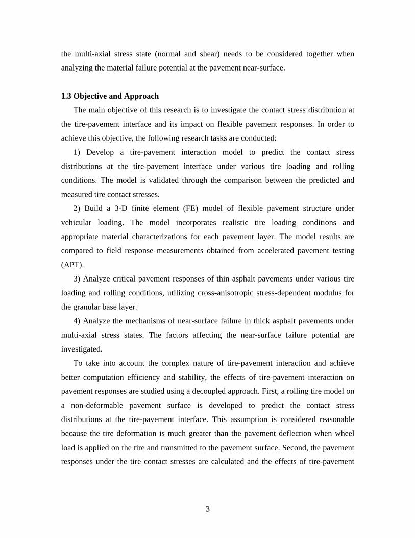
To take into account the complex nature of tire-pavement interaction and achieve
better computation efficiency and stability, the effects of tire-pavement interaction on
pavement responses are studied using a decoupled approach. First, a rolling tire model on
a non-deformable pavement surface is developed to predict the contact stress
distributions at the tire-pavement interface. This assumption is considered reasonable
because the tire deformation is much greater than the pavement deflection when wheel
load is applied on the tire and transmitted to the pavement surface. Second, the pavement
responses under the tire contact stresses are calculated and the effects of tire-pavement
4
interaction on different pavement damage mechanisms are analyzed. Figure 1.1 shows a
flowchart of the analysis approach.
Figure 1.1 Flowchart of analysis approach
1.4 Scope
This dissertation is divided into seven chapters. The first chapter introduces the
problem statement, objective, and methodology. The second chapter summarizes
previous research on mechanistic analysis of pavement responses, pavement failure
mechanisms, and tire-pavement interaction. The third chapter describes the developed
tire-pavement interaction model and analyzes the contact stress distributions at various
tire loading and rolling conditions. The fourth chapter describes the developed 3-D FE
pavement model, incorporating realistic tire loading conditions and appropriate material
Predict Tire-Pavement Contact Stresses
from Tire-Pavement Interaction Model
Non-Uniform
Vertical Stresses
Localized Tangential
Stresses
Incorporate Realistic Tire Loading into a
3-D Pavement Model
Linear Viscoelastic
Asphalt Mixture
Anisotropic and Stress-
Dependent Base
Predict Pavement Responses under Various
Tire Loading and Rolling Conditions
Develop a 3-D Tire Model and Simulate
Tire-Pavement Interaction
Composite Tire
Structure
Rolling Tire-
Pavement Contact

5
characterizations. The fifth chapter presents an analysis of thin asphalt pavement
responses utilizing nonlinear anisotropic modulus of the base layer. The sixth chapter
analyzes the near-surface failure potential of thick asphalt pavements under multi-axial
stress states. The final chapter presents analysis findings, conclusions and future study
recommendations.
6
CHAPTER 2 RESEARCH BACKGROUND
2.1 Mechanistic Analysis of Pavement Responses
2.1.1 Multilayer Elastic Theory versus Finite Element Method
The layered elastic theory is the tool used most often to calculate flexible pavement
responses to truck loading since 1940s. This is mainly due to its simplicity. The major
assumptions made in the layered elastic theory are as follows (Huang 1993):
Each layer is assumed homogeneous, isotropic, and linear elastic;
All materials are weightless (i.e., no inertia effect);
Pavement systems are loaded statically over a uniform circular area;
The subgrade is assumed to be a semi-infinite layer with a constant modulus;
The compatibility of strains and stresses is assumed to be satisfied at all layer
interfaces.
In 1943, Burmister developed a closed-form solution for a two-layered, linearly
elastic, half-space problem, which was later extended to a three-layer system. Since then,
and with advances in computer technology, the theory has been extended to deal with
multilayer systems. Accordingly, a large number of computer programs have been
developed, including BISAR, KENLAYER, ELSYM, EVERSTRESS, WESLEA, and
JULEA (Huang 1993). Some of these computer programs introduced modifications to the
original layered theory to cover viscoelastic material constitutive models (VESYS), to
allow for horizontal loading (CIRCLY), and to adjust the bonding conditions at the layer
interfaces (BISAR 3.0). However, these modifications are only accurate based upon the
validity of other assumptions.
Two-Dimensional (2-D) FE models (axisymmetric or plain strain models) were the
first successful examples of the application of the FE method in pavement analysis. The
axisymmetric modeling approach assumes that the pavement system has constant
material and geometric properties in horizontal planes, and the traffic loading is circular
load applied on the pavement surface. The plain strain model assumes a zero strain in the
z direction that is perpendicular to the xy plane of the model, when the long-bodied
structure is subjected to line loads that act in the x and/or y directions and do not vary in
the z direction. ILLI_PAVE is one of the most common software using an axisymmetric
7
FE model. In the ILLI_PAVE software, the modulus can be stress-dependent and the
Mohr-Coulomb failure criterion is used for granular materials and fine-grained soils
(Thompson and Elliott 1985).
With the advance of fast computers and algorithmic improvements, the use of 3-D FE
analysis has become widespread in pavement structural analysis (Zaghloul and White
1993). In comparison to the relatively simple layered elastic theory or 2-D axisymmetric
model, the 3-D FE model can consider many analysis scenarios, such as non-uniform tire-
pavement contact stress, irregular tire imprint area, discontinuities in pavement (cracks or
joints), viscoelastic and nonlinear material properties, infinite foundation, material
damping, quasi-static or dynamic analysis, crack propagation, coupled temperature effect,
bonded or de-bonded interface, and so forth.
2.1.2 Viscoelastic Pavement Responses under Moving Load
It is well known that the mechanical response of asphalt pavement under moving
vehicular loading is dependent on time, loading rate, and the entire loading history, due to
the viscoelastic nature of asphalt material. A number of studies since the early 1970s have
evaluated the viscoelastic responses of flexible pavements under moving loads using
different approaches.
Analytical models of viscoelastic pavement structure under a moving load vary in
complexity according to the structure analyzed (finite beam, infinite plate on Winkler
foundation, or multi-layers) and the loading (constant, harmonic, or random). The
solutions vary from analytical closed-form solutions using the corresponding principle to
semi-analytical solutions using numerical techniques. However, for complex geometries
and loading conditions, it is often impossible to get the closed-form solution from the
inverse transform.
Chou and Larew (1969) studied the multilayered pavement responses to a moving
point load based on linear viscoelastic theory. Elliot and Moavenzadeh (1971) conducted
a similar study for a circular load using an approximate approach. Huang (1973) solved
the viscoelastic pavement problem by using the approximate collocation method and
assuming a Dirichlet series for viscoelastic modulus. The influence of moving load was
assumed equivalent to that of a stationary load, with changing magnitudes depending on
8
time. A computer program (SAPSI) was developed by Sousa and coworkers (Sousa et al.,
1988) and used to compute the dynamic responses of a viscoelastic layered structure
subjected to a circular load. The total response from the moving load was obtained by the
superposition of all responses to stationary loads at a given time.
Hardy and Cebon (1993) and Papagiannakis et al. (1996) used an influence function
approach to study pavement responses to a moving load at constant speed if the pavement
response under an impulsive loading was known a priori. Hopman (1996) developed the
viscoelastic multilayer computer program (VEROAD) to calculate pavement responses
subject to moving circular loads by using the correspondence principle. In this model,
Burger’s model was used to describe the viscoelastic behavior of the asphalt material.
Siddharthan et al. (1998) used a continuum, finite-layer model (3D-MOVE) to evaluate
pavement responses under a moving surface load. The load was decomposed into
multiple single harmonic pressure distributions and the viscoelastic layer properties are
defined by the dynamic shear modulus and the internal damping ratio. Chambot et al.
(2005) developed the ViscoRoute software based on Duhamel’s semi-analytical
multilayer model to calculate pavement responses under a moving load within rectangular
or elliptic contact area. The viscoelastic behavior of the asphalt material was defined
through the Huet-Sayegh model that consists of two springs for elastic modulus and two
parabolic dampers for delayed response.
Numerical methods, such as FEM and boundary element method (BEM), have been
used to simulate pavement responses under moving vehicular loads. Pan et al. (1995)
coupled BEM with the FEM approach by modeling the elastic pavement using FE and the
underlying elastoplastic half-space using boundary elements. Yang and Hung (2001) used
2.5-D finite/infinite elements to calculate the steady state responses of pavement under a
moving load. Gonz´alez and Abascal (2004) used BEM approach and implemented the
correspondence principle to convert a viscoelastic problem to an elastic problem. Shen
and Kirkner (2001) developed a 3-D FE model based on moving coordinate system to
predict pavement residual deformation subject to moving loads. Recently, Al-Qadi and
co-workers, as well as other researchers, have used general-purpose FE software
programs to analyze viscoelastic pavement responses. In these programs, relaxation
9
moduli are usually required as the input parameters (Elseifi et al. 2006; Yoo and Al-Qadi
2008; Kim et al. 2009).
Although the 3-D FE model can be a complex and costly analysis tool, it provides the
needed versatility and flexibility to accurately simulate the nonlinear material behavior,
the complex layer interface condition, and the non-uniform distribution of tire loading.
Compared to BEM/FEM, the main advantage of analytical/semi-analytical methods is the
relatively short computational time. However, in the analytical/semi-analytical methods,
material linearity, isotropy, and no-slip interface between layers are usually assumed in
order to solve the equations.
2.1.3 Nonlinear Cross-Anisotropic Aggregate Behavior
Previous research studies have found that unbound aggregate layers exhibit stress-
and direction- (anisotropic) dependent behavior due to the nature of granular medium and
the orientation of aggregate (Uzan 1992; Tutumluer 1995). The orientation of aggregate
is controlled by its shape, compaction methods, and loading conditions. A special type of
anisotropy, known as cross-anisotropy, is commonly observed in pavement granular base
layer due to compaction and the applied wheel loading in the vertical direction.
Tutumluer and Thompson (1997) found that for a certain set of aggregate the
horizontal stiffness in the granular layer is only 3 to 21% of the vertical stiffness, and the
shear stiffness is 18 to 35% of the vertical stiffness. The nonlinear-anisotropic approach
is shown to account effectively for the dilative behavior observed under the wheel load
and the effects of compaction-induced residual stresses. The research project conducted
at the International Center for Aggregate Research (ICAR) developed a resilient modulus
testing protocol and a Systems Identification (SID) approach to determine the stress
sensitivity and cross-anisotropy of granular material (Adu-Osei et al. 2001).
Tutumluer and Seyhan (1999) used an advanced triaxial testing machine, referred as
UI-FastCell, to simulate dynamic stresses on the sample and study the effects of
anisotropic, stress-dependent aggregate behavior. Further, Seyhan et al. (2005) presented
a new methodology for determining cross-anisotropic aggregate base behavior
considering effects of moving wheel loading. The proposed testing protocol requires
conducting repeated load triaxial tests using variable confining pressure (VCP), also
10
known as the stress path tests. They found that higher vertical moduli than the horizontal
values and higher out-of-plane Poisson’s ratios than the in-plane values were typically
obtained at all stress states. In addition, the vertical moduli obtained from the negative
stress path tests were often found lower than those from the positive stress path tests,
whereas the negative stress path tests gave the highest Poisson’s ratios for both the in-
plane and the out-of-plane Poisson’s ratios.
As the pavement design method shifts from an empirical procedure to a mechanistic-
empirical (M-E) method, it is critical to consider the nonlinear anisotropic granular
behavior in the pavement response model. Tutumluer et al. (2003) and Park and Lytton
(2004) found that the nonlinear anisotropic modulus of the unbound base layer
significantly affects the stress distributions in the base layer and reduces the horizontal
tension in the bottom half of the base layer. Oh et al. (2006) and Masad et al. (2006)
showed that the FE predictions based on anisotropic models for the unbound base and
sub-base layers provide better agreements with field performance measurements. Kwon
et al. (2009) used an axisymmetric FE program (GT_PAVE) and found that the model
predictions using the nonlinear and anisotropic characterizations of the granular base
layer better capture the magnitudes and the trend in the measured response data for both
geogrid-reinforced and control low-volume flexible pavement test sections.
2.1.4 Pavement Dynamic Analysis
It is documented that structural dynamic responses or dynamic amplifications depend
on the ratio of external loading frequency to natural frequency of the structure. Although
a few researchers have studied the natural frequency of pavement structure, the range of
natural frequency was found to be 6-14 Hz for flexible pavements and 20-58 Hz for rigid
pavements (Darestani et al. 2006; Uddin and Garza 2003). Gillespie et al. (1993) found
that truck loading frequency was about 4.6Hz at a speed of 58km/h and 6.5Hz at 82km/h,
respectively. Thus, a dynamic analysis may be needed to determine pavement responses
under some loading conditions.
Researchers have used two analytical approaches to analyze transient pavement
structure response under vehicular loading. The first is using the ordinary differential
equations (ODE) developed from Newton’s second law of motion with parameters
11
characterizing the stiffness, damping, and mass of the pavement materials (Chopra 2001).
The displacements are used together with the constitutive equations to calculate the
stresses and strains in the pavement structure. The second approach is based on the
governing equations for elastodynamic wave equations (Mamlouk and Davies 1984).
These equations are used to develop the Helmholtz partial differential equation (PDE),
which is the governing equation for steady-state (harmonic) elastodynamics. In this
approach, usually, material linearity, isotropy, and no-slip between layers are assumed
and the equation can be solved with analytical and numerical techniques.
Mamlouk and Davies (1984) concluded that dynamic deflections under falling weight
deflectometer (FWD) tests were greater than the corresponding static displacements at
some locations due to local amplifications in the layered pavement structure. Lourens
(1992) showed that the stresses and deflections in the pavement differed substantially
between static and dynamic loads. They indicated that the magnitude of pavement stress
after the load passing is dependent on the loading speed. Hardy and Cebon (1994) found
that the effects of loading frequency on pavement strains are relatively minor compared
with the effect of loading speed. Zaghloul and White (1993) studied the dynamic
responses of flexible pavements and found close agreements between the results from
ABAQUS and field measurements at three different speeds.
Siddharthan et al. (1998) concluded that the dynamic effects of moving loads on
pavement strain responses are important and should not be ignored. Jooster and Lourens
(1998) found that the effect of transient pavement analysis is equally important as the
effect of non-uniform tire pressure and viscoelastic material behavior. The relative
differences between the responses from the static and dynamic models depend on the
evaluation position and material stiffness. Sadd et al. (2005) analyzed the dynamic
pavement response using an elastoplastic base and subgrade properties, and found that the
deflection under the dynamic load condition is less than its corresponding value obtained
from the static analysis. They concluded that this result was expected, since in the
dynamic analysis, inertial, dissipative, and internal forces absorbed the work done by
externally applied forces. Yoo and Al-Qadi (2007) found that compared to quasi-static
analysis, the dynamic transient analysis induces greater strain responses and residual
strains after load passing.
12
2.1.5 Effect of Tire Contact Stresses on Pavement Responses
Research has shown that the assumed distribution of tire-pavement contact stresses
significantly affects pavement responses. Most researchers analyzed the effect of contact
stress distributions on pavement responses using an elastic approach. Prozzi and Luo
(2005) found that the tensile strains in the asphalt layer under actual contact stresses were
quite different from those under uniform contact stresses, depending on the combination
of load and tire inflation pressure. Similarly, Machemehl et al. (2005) reported that the
conventional uniform load assumption underestimated pavement responses at low tire
inflation pressures and overestimated pavement responses at high tire pressures. De Beer
et al. (2002) observed that pavement responses of thin flexible pavements were sensitive
to vertical load shape and distribution. Soon et al. (2004) found that the tangential tire
stresses caused tensile stresses outside the tire treads and their locations and magnitudes
depended on the pavement thickness. Park et al. (2005) concluded that the predicted
pavement fatigue life under the modified uniform load assumption (using measured tire
contact area) showed better agreement with the predicted fatigue life under measured tire
contact stresses, compared to the conventional uniform load assumption. Thyagarajan et
al. (2009) also noted that the load-strain linear proportionality assumption in the MEPDG
led to significant error in the predicted permanent deformation in the upper pavement
layer.
Recently, some researchers analyzed the effect of contact stress distributions on
viscoelastic pavement responses under moving loads. Siddharthan et al. (2002) showed
that the difference between the responses computed with the uniform and non-uniform
tire-pavement contact stress distributions is in the range of 6-30%. In this study, the effect
of tangential contact stresses was not considered. Al-Qadi and Yoo (2007) reported that
the effect of surface tangential contact stresses cannot be neglected because it may greatly
affect pavement responses near the asphalt surface layer, and this effect diminishes as the
depth increases. Wang and Al-Qadi (2009) found that the non-uniform distribution of
vertical contact stresses and transverse tangential stresses induce outward shear flow from
tire center and the shear strain concentration under tire ribs at the near-surface of thick
asphalt pavements.
13
In summary, the literature review revealed important differences between the critical
pavement responses when the assumptions of contact stress distributions change. The
actual tire-pavement contact stresses induce greater or smaller pavement responses,
compared to the conventional uniform contact stress distribution, depending on tire load
and pressure, material stiffness, pavement thickness, and the type of response for
comparison. These differences can only be accurately accounted for by utilizing a
modeling approach that can simulate realistic contact stress distributions at the tire-
pavement interface and predict viscoelastic pavement responses under moving vehicular
loading.
2.1.6 Impact of New Generation of Wide-Base Tires
Various combinations of tire sizes and types are currently used on trucks. These truck
tires have widths from 285mm to 495mm. Normally, tires with widths of less than
315mm are used as dual-tire assembly (except on steering axles) while those with widths
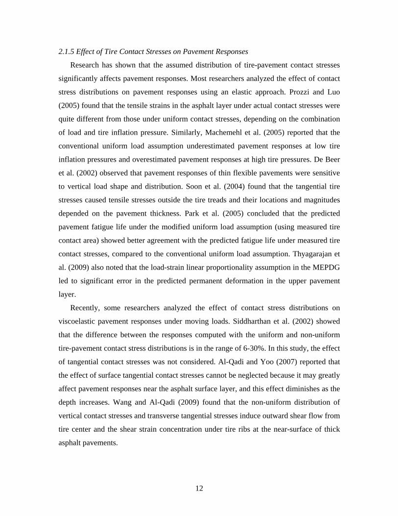
of more than 315mm can be used as single tires. The nomenclature of tires usually
includes three tire dimensions and types of tire in the form of AAA/BBXCC.C. The first
number (AAA) is the tire width from wall-to-wall in mm or inch, the second number
(BB) is the sidewall height given as a percentage of the tire width. The letter (X) indicates
the type of tire (radial or bias ply). The third number (CC.C) is the tire rim diameter in
inches. For example, a tire designation 455/55R22.5 is a radial tire (indicated with the
“R”), with a wall-to-wall width of 455mm, a wall height of 250mm, and a rim diameter
of 22.5in (571.5mm) (Figure 2.1).
Figure 2.1 Comparisons of different tire configurations (after Michelin product bulletin,
2006)
14
Traditionally, dual-tire assembly has been used to provide an adequate footprint to
carry heavy loads and to distribute axle load over a large area on the pavement surface.
Compared to the conventional dual-tire assembly, it is reported that wide-base tires can
improve fuel efficiency, reduce emissions, increase payload, exhibit superior braking and
comfort, and reduce tire repair, maintenance, and recycling cost (Al-Qadi and Elsefi
2007). However, the first generation of wide-base tires (385/65R22.5 and 425/65R22.5)
produced in the early 1980s were found to cause 1.5 to 2.0 times more rut depth and 2.0
to 4.0 times more fatigue cracking than a dual-tire assembly when carrying the same load.
This has led many transportation agencies to discourage their use.
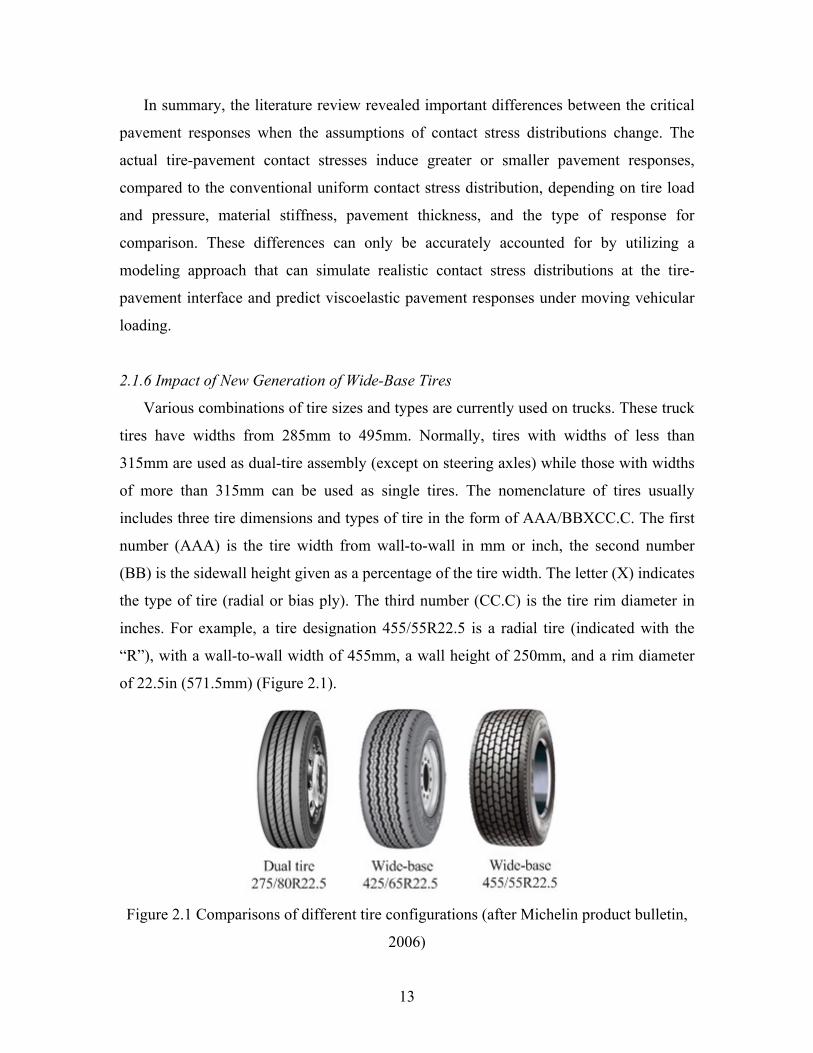
The new generation of wide-base tires (445/50R22.5 and 455/55R22.5) came to
market in the 2000’s in order to reduce pavement damage and provide other safety and
cost-saving advantages. The new generation of wide-base tires are 15 to 18% wider than
the first generation and do not require high tire inflation pressure due to their special wall
designs (Al-Qadi et al. 2005). Figure 2.2 shows the evolution of wide-base tire
technology. Over the years, wide-base tires have become increasingly wider than their
predecessors.
NA: Designed for North America, EU: Designed for the European Union
Figure 2.2 Evolution of wide-base tires (after Al-Qadi et al. 2005)
The impact of the new generation of wide-base tires on pavement damage was
investigated by Al-Qadi and co-workers first in 2000. A comprehensive study was
conducted to compare the pavement responses under wide-base tires and the dual-tire
275mm
Dual
570mm
425mm385mm 445/455mm
Wide-Base Wide Base -NA
495mm
Wide Base -EU 2000
Wide-Base 1980 1980 2000/2002
15
assembly on the heavily instrumented Virginia Smart Road. The study considered several
pavement designs, truck speeds, loads, as well as tire pressure levels. Studies were also
conducted by Al-Qadi and co-workers to investigate the pavement damage mechanisms
induced by different tire configurations using a 3-D FE model. They concluded that the
new wide-base 455 tire could cause greater or less pavement damage potential than the
dual-tire assembly, depending on the pavement structure and failure mechanism (Al-Qadi
et al. 2002; Al-Qadi et al. 2005, Yoo and Al-Qadi 2008; Al-Qadi and Wang 2009).
The COST Action 334 study conducted in Europe (2001) indicated that the new
generation of wide-base tires would cause approximately the same primary rutting
damage as a dual-tire assembly on primary roads and 44 to 52% more combined damage
(20% primary rutting, 40% secondary rutting, and 40% fatigue cracking) on secondary
roads. The COST study was mainly based on the field monitoring of pavement responses
and performance. Pierre et al. (2003) conducted field measurements and found that the
wide-base 455 tire caused more distortions at the pavement base in the spring but similar
distortions in the summer, as compared to the dual tires. The wide-base 455 tire was also
found to cause less primary rutting than the dual-tire assembly. Priest and Timm (2006)
found from field measurements that the new wide-base 445 tire resulted in a similar
pavement fatigue life as the standard dual-tire assembly (275/80R22.5); while the
contrary conclusion was obtained when using the linear elastic analysis. This indicates
that the layered elastic theory may not be appropriate to accurately compare pavement
responses caused by different tire configurations. Greene et al. (2010) evaluated the
pavement damage caused by various tire configurations using the accelerated pavement
testing. The investigation revealed that the wide-base 455 tire performed as well as the
dual tire assembly. The wide-base 445 tire was shown to create more rut damage on a
dense-graded pavement surface and was predicted to create more bottom-up cracking
than a dual-tire assembly.
The aforementioned studies indicate that the impact of wide-base tires on pavement
damage depends on the pavement structures, pavement failure mechanisms considered,
and environmental conditions. Generally, the damage caused by wide-base tires decreases
as the tire width increases.
16
2.2 Pavement Failure Mechanisms
2.2.1 Conventional Asphalt Pavement Failures
Pavement failure may occur as a result of the environment, repeated traffic loading,
deficient construction, and/or poor maintenance strategies. The two main load-associated
distresses with flexible pavements are rutting and fatigue cracking.
Bottom-Up Fatigue Cracking
Fatigue cracking is caused by repeated relatively heavy load applications, usually
lower than the strength of the paving material. Bottom-up fatigue cracking usually starts
at the bottom of the asphalt layers of relatively thin flexible pavements (less than 150mm)
or at the bottom of the individual asphalt layer if poor bonding conditions exist (Yoo and
Al-Qadi 2008). The proposed AASHTO MEPDG determines the number of allowable
load applications for fatigue cracking using Equation 2-1 (ARA 2004). This method
utilizes the initial pavement response and ignores the evolution of strains with damage.
However, the introduced error is considered acceptable within the empirical design
framework.
281.1
9492.3 1)1(00432.0
⋅⋅⋅=
ECkN
tf ε
(2-1)
where fN is the number of allowed load applications; E is the resilient modulus of
asphalt mixture (in psi); tε is the tensile strain at the bottom of asphalt layer; C is a
parameter related to asphalt mixture volumetric properties; and k is a parameter related
to asphalt layer thickness.
Recently, more advanced fatigue models have been proposed based on viscoelastic
continuum damage theory, dissipated energy concept, and viscoelastic fracture mechanics
(Daniel and Kim 2002; Shen and Carpenter 2007; Kuai et al. 2009). These approaches are
inherently more complex and offer more fundamental explanations than the empirical
fatigue approach. Thus, they are applicable to predict fatigue damage growth in asphalt
mixtures under a broader range of loading and environmental conditions and consider the
effects of viscoelastic properties and fracture characteristics, such as binder aging and
healing effects.
17
Primary Rutting
Rutting is the permanent deformation occurring in the pavement structure, including
rutting in asphalt layers (primary rutting), rutting in unbound base layers, and subgrade
(secondary) rutting. Primary rutting in asphalt layers includes two types of deformation:
volume reduction caused by traffic densification, and permanent movement at a constant
volume or dilation caused by shear flow. The general form of primary rutting models is
usually derived from statistical analysis of the relationship between plastic and elastic
compressive strains measured from repeated-load uniaxial/triaxial tests. The following
transfer function is suggested by the AASHTO 2002 MEPDG, Equation 2-2 (ARA 2004).
)log(02755.2)log(4262.07498.3)log( TNr
p ++−=εε
(2-2)
where pε is the accumulative permanent strain; rε is the recoverable strain; N is the
allowed number of load repetitions corresponding to pε ; and T is the pavement
temperature (°C).
Monismith et al. (1994) demonstrated that the accumulation of permanent
deformation in the asphalt layer is very sensitive to the layer’s resistance to shape
distortion (i.e., shear) and relatively insensitive to volume change. Their study indicates
that the rutting in asphalt layers is caused principally by shear flow rather than volumetric
densification; especially under loading of slow moving vehicles at high temperature.
Deacon et al. (2002) and Monismith et al. (2006) correlated the rutting in asphalt layers to
shear stresses and shear strains in the asphalt layer instead of compressive strains, as
shown in Equation 2-3. This model was originally developed for Westrack mixes based
on repeated simple shear test at constant height (RSST-CH). ce
s nba γτγ )exp(⋅= (2-3)
where γ is the permanent (inelastic) shear strain; eγ is the elastic shear strain; sτ is the
corresponding shear stress; n is the number of axle load applications; and a , b , and c
are experimentally determined coefficients.
18
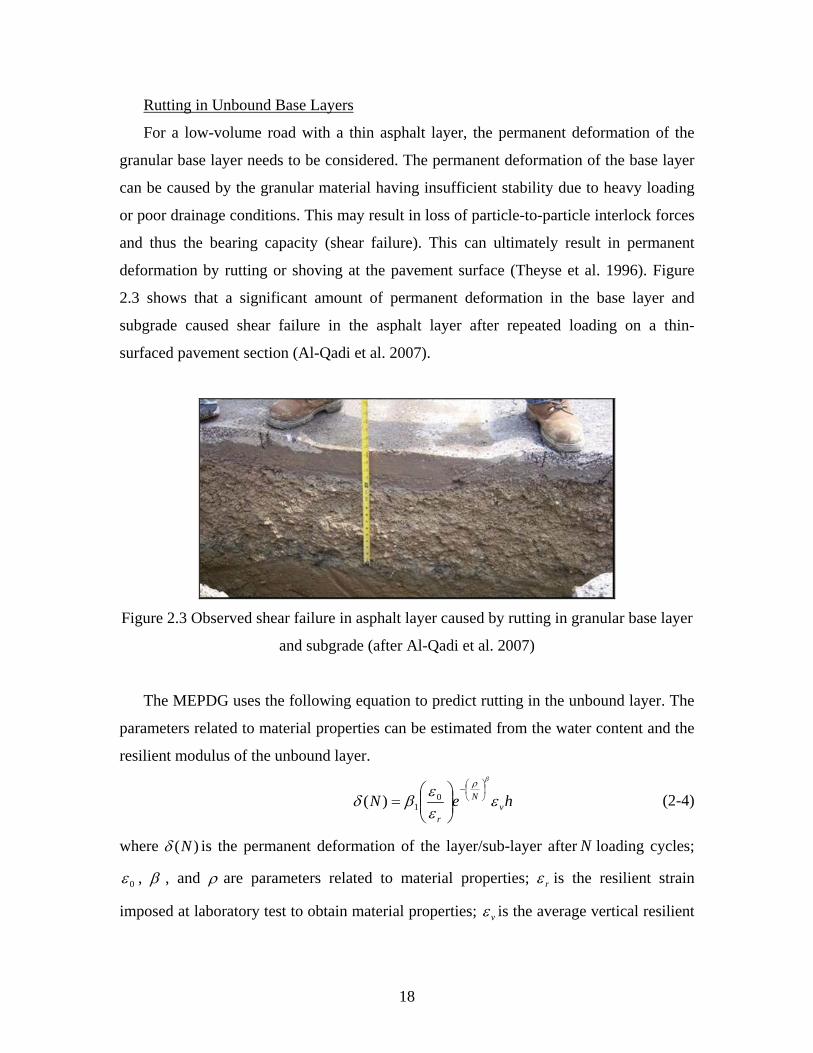
Rutting in Unbound Base Layers
For a low-volume road with a thin asphalt layer, the permanent deformation of the
granular base layer needs to be considered. The permanent deformation of the base layer
can be caused by the granular material having insufficient stability due to heavy loading
or poor drainage conditions. This may result in loss of particle-to-particle interlock forces
and thus the bearing capacity (shear failure). This can ultimately result in permanent
deformation by rutting or shoving at the pavement surface (Theyse et al. 1996). Figure
2.3 shows that a significant amount of permanent deformation in the base layer and
subgrade caused shear failure in the asphalt layer after repeated loading on a thin-
surfaced pavement section (Al-Qadi et al. 2007).
Figure 2.3 Observed shear failure in asphalt layer caused by rutting in granular base layer
and subgrade (after Al-Qadi et al. 2007)
The MEPDG uses the following equation to predict rutting in the unbound layer. The
parameters related to material properties can be estimated from the water content and the
resilient modulus of the unbound layer.
heN vN
r
εεεβδ
βρ
−
= 0
1)( (2-4)
where )(Nδ is the permanent deformation of the layer/sub-layer after N loading cycles;
0ε , β , and ρ are parameters related to material properties; rε is the resilient strain
imposed at laboratory test to obtain material properties; vε is the average vertical resilient
19
strain calculated from the primary response model; h is the thickness of the layer/sub-
layer; and 1β is the calibration factor.
The South African Mechanistic Design Method (SA-MDM) takes into account the
permanent deformation of the base layer, as shown in Equations 2-5 and 2-6 (Theyse et al.
1996). The permanent deformation is related to the ratio of the working stress to the yield
strength of the material, considering that high shear stress can extend into the base layer
in thin-surfaced pavements for normal traffic loading.
31
23 )
245tan(2]1)
245((tan[
σσ
φφσ
−
++−+=
kckF (2-5)
)480098.3605122.2(10 += FN (2-6)
where F is the calculated safety factor; 1σ and 3σ are the major and minor principal
stresses (compressive stress positive and tensile stress negative); k is a constant
depending on the moisture condition; c is the cohesion coefficient; φ is the angle of
internal friction; and N is the number of allowed load applications until failure.
Recently, Kim and Tutumluer (2005) developed a permanent deformation model of
unbound aggregate considering the static and dynamic stress states and the slope of stress
path loading. They found that multiple stress path tests could simulate the extension–
compression–extension type of rotating stress states under a moving wheel pass and give
much higher permanent strains than those of the compression-only single path tests.
Subgrade Rutting
Subgrade rutting is a longitudinal wheel-path depression that occurs when the
subgrade exhibits permanent deformation or lateral migration due to loading. In this case,
the pavement settles into the subgrade ruts, causing surface depressions in the wheel path.
Usually, the vertical compressive strain on top of the subgrade is related to subgrade
rutting for the case that the shear capacity of subgrade soil is not exceeded by the applied
load. The Asphalt Institute (1982) proposed a rutting damage model, based on roadbed
soil strain with a maximum threshold of 12.5mm rutting on subgrade (Equation 2-7). 477.49 )(10365.1 −−×= vN ε (2-7)
20
where N is the number of allowed load repetitions until failure, and vε is the maximum
vertical compressive strain on top of the subgrade.
Subgrade soil can also fail in shear when its shear capacity is exceeded by the applied
heavy load. Thompson (2006) used a parameter called subgrade stress ratio (SSR) to
estimate the rutting potential of a pavement system. The SSR is defined by Equation 2-8.
The subgrade damage potential limits are SSR = 0.5, 0.6, 0.6-0.75, and >0.75 for low,
acceptable, limited, and high ratios, respectively.
udev qSSR /σ= (2-8)
where SSR is the subgrade stress ratio; devσ is the deviatoric stress at the top of the
subgrade; and uq is the unconfined compressive strength of the subgrade soil.
2.2.2 Near-surface Cracking in Thick Asphalt Pavement
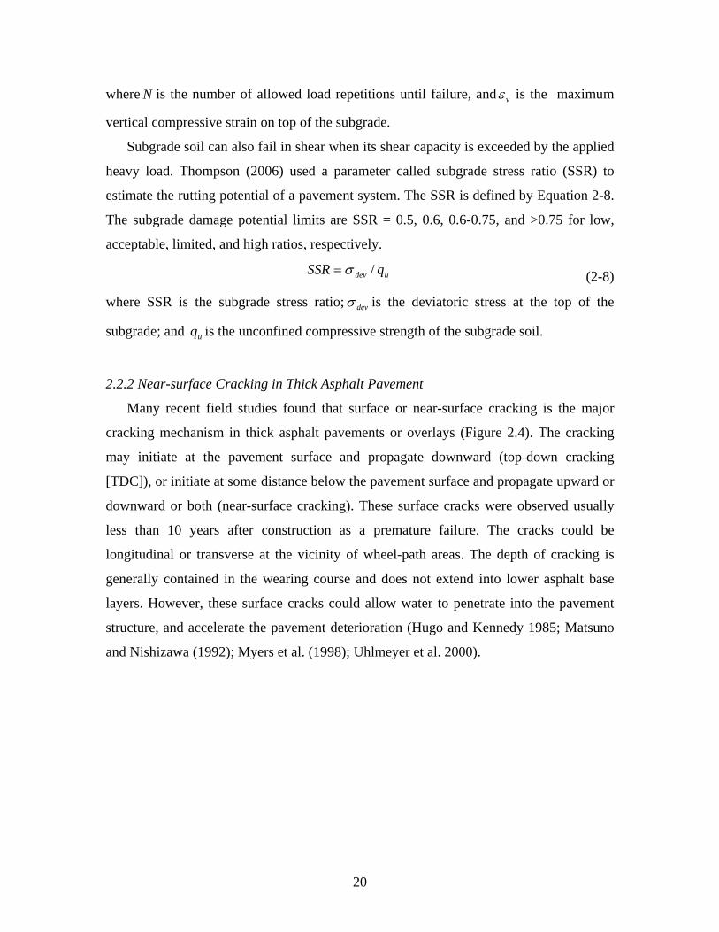
Many recent field studies found that surface or near-surface cracking is the major
cracking mechanism in thick asphalt pavements or overlays (Figure 2.4). The cracking
may initiate at the pavement surface and propagate downward (top-down cracking
[TDC]), or initiate at some distance below the pavement surface and propagate upward or
downward or both (near-surface cracking). These surface cracks were observed usually
less than 10 years after construction as a premature failure. The cracks could be
longitudinal or transverse at the vicinity of wheel-path areas. The depth of cracking is
generally contained in the wearing course and does not extend into lower asphalt base
layers. However, these surface cracks could allow water to penetrate into the pavement
structure, and accelerate the pavement deterioration (Hugo and Kennedy 1985; Matsuno
and Nishizawa (1992); Myers et al. (1998); Uhlmeyer et al. 2000).
21
Figure 2.4 Observed top-down cracking in field (after Uhlmeyer et al., 2000)
Several factors have been proposed as the causes of TDC or near-surface cracking.
These include load-induced factors (tension, shear), material factors (low fracture
energies, aging), construction factors (longitudinal construction joints, segregation); and
temperature-induced factors (thermal stress) (Baladi et al. 2002). Among these factors,
the high tensile or shear stress induced by tires at the pavement surface or near-surface is
the most well-recognized load factor that contributes to the surface cracking mechanism.
The repetitive load-induced tensile/shear stress could initiate the material damage process,
while the thermal stress during daily thermal cycles accelerates the damage evolution and
the asphalt aging reduces its fracture energy and fatigue life.
Myers et al. (1998) concluded that tensile stresses under the ribs of the loaded tire at
the pavement surface induced by the shear stress of radial tires were responsible for
causing TDC. It was found that the pavement structure has little effect on the reduction of
tensile stresses around the tire-pavement contact area. Groenendijk (1998) found that the
combined influence of the non-uniform contact stress and the aging of the asphalt surface
layer could result in critical tensile stress at the surface rather than the bottom of the
asphalt layer. Thom (2003) found that the value of the maximum principal tensile strain
at 10mm below the pavement surface (at approximate 45° to surface) can be of a similar
magnitude to the horizontal tensile strain at the bottom of asphalt layer, particularly for a
thick pavement structure.
Wang et al. (2003) analyzed the cause of top-down cracking from the
micromechanics point of view and found that the secondary tensile stress could be
22
induced by the shear loading due to dilation. They suggested that the aggregate particle
skeleton structure and the strength of the mastics are two important factors that may
affect top-down cracking. Wang et al. (2006) found that the load-induced viscoelastic
residual stress may be another potential mechanism for TDC using viscoelastic boundary
element method. Yoo and Al-Qadi (2008) and Al-Qadi et al. (2008) showed that the
vertical shear strain at the tire edge is more critical than the tensile strain at the bottom of
asphalt layer for thick asphalt pavement and could be responsible for the development of
near-surface cracking.
The literature survey shows that few fatigue models consider the combined effect of
tensile and shear stress/strain on the prediction of surface or near-surface cracking. The
MEPDG uses the elastic layer theory and the static uniform circular loading assumption
to compute the tensile strains near the pavement surface for predicting the surface-
initiated fatigue cracks (ARA 2004). The proposed fatigue equation for surface cracking
is similar to the one for bottom-up fatigue cracking (Equation 2-1), while it has a
different definition of the correction factor ( k ). However, the rationality and accuracy of
this method is still not verified.
Lytton (1993) developed a cracking initiation model in the Strategic Highways
Research Program (SHRP) research and found that the number of load cycles to reach
failure could be predicted with excellent accuracy by taking into account the original
stiffness, the state of stress expressed in terms of the mean principal stress and the
octahedral shear stress at the bottom of the beam, and the percent air void and asphalt
binder in the mix. Sousa el al. (2005) proposed the concept of “von Mises strain” to
consider the normal and shear strain together and calculated the overlay fatigue life from
flexural fatigue test with controlled strain (Equation 2-9).
[ ]232
221
231 )()()(
21 εεεεεεε −+−+−=VM (2-9)
where )1(1 vVM += εε for beam fatigue test conditions subjected to a four-point bending.
The researchers at the University of Florida proposed an Energy Ratio (ER) concept
to calculate the optimum pavement thickness for resisting TDC. The ER is a
dimensionless parameter defined as the dissipated creep strain energy ( fDSCE ) threshold
23
of the mixture divided by the minimum required dissipated creep strain energy ( minDSCE )
(Equation 2-10). The DSCE is the total energy under the stress-strain curve minus the
elastic energy. The minimum required DCSE was derived from the material properties
and structure design effect and calibrated with the observed cracking performance in the
field (as shown in Equations 2-11 and 2-12). It is assumed that when ER is greater than
one, a macro-crack will initiate and the process is not reversible.
min/ DCSEDCSEER f= (2-10)
),( max
198.2
min σtSfDmDCSE ⋅
= (2-11)
81.3max 1046.2
44.3336.6),(
max
−×+⋅−
=σ
σ tt
SSf (2-12)
where tS is the tensile strength (in MPa); maxσ is the maximum tensile stress (in psi);
and 0D and 1D are the creep parameters in the expression mtDDtD 10)( += .
The recent completed National Cooperative Highway Research Program (NCHRP)
study (Roque et al. 2010) recognizes the top-down cracking could be caused by bending-
induced surface tension away from the tire in asphalt layers of thin to medium thickness,
or shear-induced near-surface tension at the tire edge in thicker asphalt layers. In this
study, a viscoelastic continuum damage model and a fracture mechanics model are used
to predict crack initiation and propagation, respectively. However, the developed model
is still not suitable for integration and development of a top-down cracking performance
prediction model for the mechanistic-empirical design.
2.3 Tire-Pavement Interaction
2.3.1 Measured Tire-Pavement Contact Area and Stresses
Tires serve many important purposes for a traveling vehicle including cushioning the
vehicle against road roughness, controlling stability, generating maneuvering forces, and
providing safety, among others (Gillespie 1993). Tire-pavement interaction is important
for pavement design because the tire imprint area is the only contact area between the
vehicle and the pavement at which the actual distribution of contact stresses is transferred
to the pavement surface.
24
There are two important factors in the tire-pavement interaction mechanism: the
contact area and the contact stresses. Many researchers have used a circular or equivalent
rectangular contact area in pavement loading analysis (Huang 1993). The contact area of
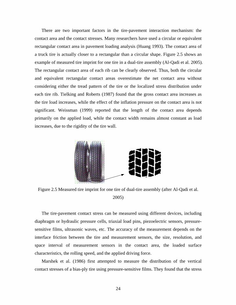
a truck tire is actually closer to a rectangular than a circular shape. Figure 2.5 shows an
example of measured tire imprint for one tire in a dual-tire assembly (Al-Qadi et al. 2005).
The rectangular contact area of each rib can be clearly observed. Thus, both the circular
and equivalent rectangular contact areas overestimate the net contact area without
considering either the tread pattern of the tire or the localized stress distribution under
each tire rib. Tielking and Roberts (1987) found that the gross contact area increases as
the tire load increases, while the effect of the inflation pressure on the contact area is not
significant. Weissman (1999) reported that the length of the contact area depends
primarily on the applied load, while the contact width remains almost constant as load
increases, due to the rigidity of the tire wall.
Figure 2.5 Measured tire imprint for one tire of dual-tire assembly (after Al-Qadi et al.
2005)
The tire-pavement contact stress can be measured using different devices, including
diaphragm or hydraulic pressure cells, triaxial load pins, piezoelectric sensors, pressure-
sensitive films, ultrasonic waves, etc. The accuracy of the measurement depends on the
interface friction between the tire and measurement sensors, the size, resolution, and
space interval of measurement sensors in the contact area, the loaded surface
characteristics, the rolling speed, and the applied driving force.
Marshek et al. (1986) first attempted to measure the distribution of the vertical
contact stresses of a bias-ply tire using pressure-sensitive films. They found that the stress
25
distributions are not uniform, and that the vertical pressures exceed the inflation pressure
in some areas. Ford and Yap (1990) measured the contact stresses for a slow-rolling tire
over a strain gauge transducer embedded in the flat road bed with the use of a specially
instrumented flat bed device. They found that, at a constant load, the tire inflation
pressure variation primarily affects the contact stresses in the central region of the contact
area. In contrast, at a constant inflation pressure, the tire load variation explicitly
influences the contact stresses in the outer regions of the contact area.
Tielking and Abraham (1994) used an MTS servo-hydraulic system and triaxial load
pins to measure the vertical contact stresses under tires and emphasized the cantilever
effect caused by the usual offset flange wheel in heavy trucks. De Beer et al. (1997)
performed a comprehensive measurement of tire contact stresses using the Vehicle-Road
Surface Pressure Transducer Array (VRSPTA), that is further developed as Stress-in-
Motion System (SIM). Their data have been used by many researchers to predict
pavement responses. The VPSPTA consists mainly of an array of tri-axial strain gauge
steel pins fixed to a steel base plate, together with additional non-instrumented supporting
pins, fixed flush with the road surface. This system is designed to take measurements at
wheel speeds from 1km/h up to 25km/h, and loads up to 200kN (vertical) and 20kN
(horizontal). It was observed that the ratio of maximum stresses in the vertical, transverse,
and longitudinal directions is 10: 3.6: 1.4 for a smooth bias ply tire.
Myers et al. (1999) reported that the radial tire causes higher transverse stresses than
the bias ply tire, and the wide-base Bridgestone M844 tire has the highest vertical and
transverse stresses. They also found that the bias ply tire has the maximum vertical stress
at the shoulders of the tire, while the radial tire has the maximum vertical stress at the
center of the tire which could be as high as 2.3 times the tire inflation pressure. The
transverse shear stresses under the tire are affected by both the pneumatic effect and the
Poisson’s effect. Poisson’s effect was more significant for radial tires, which have more
flexible sidewalls and rigid treads than bias ply tires. Douglas et al. (2000) developed a
steel bed transducer array device to measure vertical and tangential contact stresses for
use in the evaluation of surface chip damage. They found that vertical contact stresses
under the tire are extremely non-uniform under heavy loads with low inflation pressure,
26
and that longitudinal contact stresses at the trailing edge of the tire contact patch are
significantly greater when the inflation pressure was low.
2.3.2 Background on Tire Models
The two main types of tires are bias-ply and radial-ply tires. The radial-ply tire has
become more popular because it causes less rolling resistance and heat generation
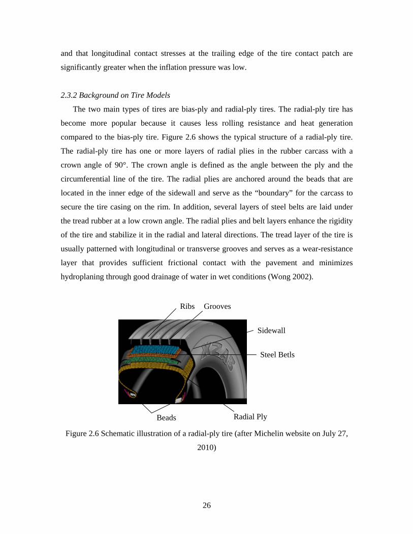
compared to the bias-ply tire. Figure 2.6 shows the typical structure of a radial-ply tire.
The radial-ply tire has one or more layers of radial plies in the rubber carcass with a
crown angle of 90°. The crown angle is defined as the angle between the ply and the
circumferential line of the tire. The radial plies are anchored around the beads that are
located in the inner edge of the sidewall and serve as the “boundary” for the carcass to
secure the tire casing on the rim. In addition, several layers of steel belts are laid under
the tread rubber at a low crown angle. The radial plies and belt layers enhance the rigidity
of the tire and stabilize it in the radial and lateral directions. The tread layer of the tire is
usually patterned with longitudinal or transverse grooves and serves as a wear-resistance
layer that provides sufficient frictional contact with the pavement and minimizes
hydroplaning through good drainage of water in wet conditions (Wong 2002).
Radial PlyBeads
Steel Betls
Ribs
Sidewall
Grooves
Figure 2.6 Schematic illustration of a radial-ply tire (after Michelin website on July 27,
2010)
27
Simplified 2-D tire models have been used in vehicle dynamics to predict tire
performance in traction and stability control (Knothe et al. 2001). The common 2-D tire
models can be divided into three main groups. The first group consists of the classical
spring-damper models with single contact point with the road surface. The second group
is the tire-ring models, which have an outer contour in contact with the ground. The third
group consists of parametric mathematic models, such as the Pacjeka model. These
models are derived from measurements of testing tires under various conditions.
However, they are usually unsuitable for quantitative prediction of tire-pavement contact
stresses in the tire imprint area.
General-purpose FE commercial software, such as ABAQUS, ANSYS, and ADINA,
provide more tools to simulate 3-D tire behavior with rolling contact. The FE method is
preferred because it can simulate the complex tire structure (tread, sidewall, radial ply,
belt, bead, etc.) and consider representative material properties of each tire component. A
survey of existing literature reveals many published works on FE simulations of tires.
The complexity of tire models varies, depending on the features built into the model,
including the types of FE formulation (Lagrangian, Eulerian, or Arbitrary Lagrangian
Eulerian), material models (linear elastic, hyperelastic, or viscoelastic), type of analysis
(transient or steady state), and treatment of coupling (isothermal, non-isothermal, or
thermo-mechanical). Such tire models can be used to analyze the energy loss (rolling
resistance), tire-terrain interaction, vibration and noise, and tire failure and stability.
The contact stresses developed at the tire-pavement interface are usually studied by
assuming a deformable tire on a rigid surface. Tielking and Robert (1987) developed a FE
model of a bias-ply tire to analyze the effect of inflation pressure and load on tire-
pavement contact stresses. The pavement was modeled as a rigid flat surface and the tire
was modeled as an assembly of axisymmetric shell elements positioned along the carcass
mid-ply surface. Roque et al. (2000) used a simple strip model to simulate the cross-
section of a tire and concluded that the measurement of contact stresses using devices
with rigid foundation was suitable for the prediction of pavement responses. Zhang (2001)
built a truck tire model using ANSYS and analyzed the inter-ply shear stresses between
the belt and carcass layers as a function of normal loads and pressures.
28
Meng (2002) modeled a low profile radial smooth tire on rigid pavement surface
using ABAQUS, and analyzed the vertical contact stress distributions under various tire
loading conditions. Ghoreishy et al. (2007) developed a 3-D FE model for a 155/65R13
steel-belted tire and carried out a series of parametric analyses. They found that the belt
angle was the most important constructional variable for tire behavior and the change of
friction coefficient had great influence on the pressure field and relative shear between
tire treads and road.
On the other hand, the assumption of a fully rigid wheel has been employed
extensively in soil-wheel (or vehicle-terrain interaction) in the field of terramechanics.
The geometry of a wheel is simplified to a rigid cylinder and the soil beneath the rolling
wheel is usually assumed to be plastic. In these applications, the main objective is to
predict the relationship between the wheel penetration or traction and the applied vertical
force, torque, wheel geometry, material properties, and interface friction at the soil-wheel
interface. Shoop (2001) simulated the coupled tire-terrain interaction and analyzed the
plastic deformation of soft soil/snow using an Arbitrary Lagrangian Eulerian (ALE)
adaptive mesh formulation. He suggested that the assumption of a rigid tire may be
suitable for soft terrain analysis.
Hambleton and Drescher (2007) predicted the load-penetration relationships for
indentation and steady-state rolling of rigid cylindrical wheels on cohesive soils and
found good agreement between the theoretical predictions and experimental
measurements. Hambleton and Drescher (2009) further studied the inclined rolling force
and wheel sinkage using a three-dimensional model. They found that sinkage is inversely
proportional to the width of the wheel and the wheel diameter. These findings are
particularly useful for evaluating the “test rolling” procedure used for assessing the
quality of subgrade compaction and optimizing the traction performance (or tire mobility)
of off-road vehicles on unpaved roads.
2.3.3 Rolling Tire-Pavement Contact Problem
The tire-pavement interaction is essentially a rolling contact problem. Several
challenges exist when modeling the tire-pavement interaction via a two-solid contact
mechanics approach, such as nonlinear material properties, transient contact conditions,
29
intricate structure of the tire, and nonlinear frictional interface (Laursen and Stanciulescu
2006). Due to the complexity of the problem, it is difficult to solve the tire-pavement
contact problem analytically. Numerical methods are necessary and FEM is usually an
appropriate choice.
In computational mechanics, two classical descriptions of motion are available: the
Lagrangian formulation and the Eulerian formulation. The Eulerian formulation is widely
used in fluid mechanics; the computational mesh is fixed and the continuum moves with
respect to the mesh. The Lagrangian formulation is mainly used in solid mechanics; in
this description each individual node of the computational mesh follows the associated
material particle during the motion. However, it is cumbersome to model rolling contact
problem using a traditional Lagrange formulation since the frame of reference is attached
to the material. In this reference frame, a steady-state tire rolling is viewed as a time-
dependent process and each point undergoes a repeated process of deformation. Such an
analysis is computationally expensive because a transient analysis must be performed for
each point and fine meshing is required along the entire tire surface (Faria et al. 1992).
An Arbitrary Lagrangian Eulerian (ALE) formulation combines the advantages of the
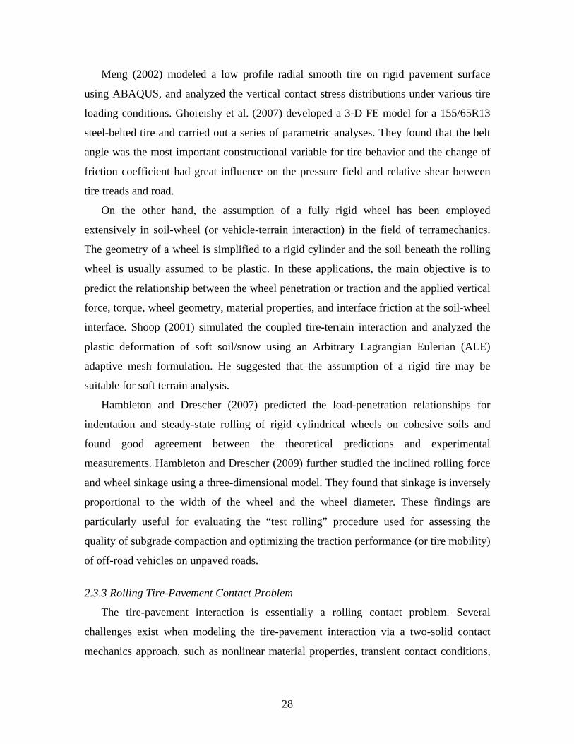
Lagrangian and Eulerian formulations for solving the steady-state tire rolling problem
(Hughes et al. 1981; Nackenhorst 2004). The general idea of ALE is the decomposition
of motion φ into a pure rigid body motion, denoted by the mapping χ , and the
superimposed deformation, denoted by φ̂ , as shown in Figure 2.7. This kinematic
description converts the steady moving contact problem into a pure spatially dependent
simulation. Thus, the mesh needs to be refined only in the contact region and the
computational time can be significantly reduced.
30
Figure 2.7 Arbitrary Lagrangian Eulerian decomposition of motion (after
Nackenhorst 2004)
Another crucial point in the solution of the rolling contact problem is a sound
mathematical description of the contact conditions. Contact problems are nonlinear
problems and they are further complicated by the fact that the contact forces and contact
patches are not known a priori. A solution to contact problems must satisfy general basic
equations, equilibrium equations and boundary conditions, like solutions for a solid
mechanics problem.
The popular approach to solve the contact problem is to impose contact constraint
conditions using nonlinear optimization theory. Several approaches are used to enforce
non-penetration in the normal direction, amongst which the most used are the penalty
method, the Lagrange multipliers method or the augmented Lagrangian method
(Wriggers 2002). If there is friction between two contacting surfaces, the tangential
forces due to friction and the relative stick-slip behavior needs to be considered. The
frequently used constitutive relationship in the tangential direction is the classical
Coulomb friction law. This model assumes that the resistance to movement is
proportional to the normal stress at an interface. In this case, the interface may resist
movement up to a certain level; then the two contacting surfaces at the interface start to
slide relative to each another. If the relative motion occurs, the frictional stress remains
constant and the stress magnitude is equal to the normal stress at the interface multiplied
by the friction coefficient.
31
2.3.4 Friction at Tire-Pavement Interface
The development of friction force between tire rubber and a rough hard surface has
two contributions that were commonly described as the adhesion and hysteretic
deformation, respectively. The adhesion component is the result of interface shear and
more important for a clean and smooth surface. The magnitude of adhesion component is
related to the product of actual contact area and the interface shear strength. The
hysteresis component is the result of damping losses and energy dissipation of the rubber
excited by the surface asperities (Kummer and Meyer 1969).
Because the mechanics of rubber friction are very complex as a consequence of many
interacting phenomena, the friction behavior between the tire and pavement is usually
determined experimentally. Pavement friction is defined as the retarding tangential force
developed at the tire-pavement interface that resists longitudinal sliding when braking
forces are applied to the vehicle tires or sideways sliding when a vehicle steers around a
curve. The sliding friction coefficient is computed using Equation 2-13.
vh FF /=µ (2-13)
where µ is sliding friction coefficient; hF is tangential friction force at the tire-pavement
surface; and vF is vertical load on tire.
The type of equipment used for testing tire-pavement friction varies among
transportation agencies. Common techniques include the locked wheel tester using a
smooth or ribbed tire, fixed slip device, variable slip device, and side force device.
Experimental measurements have shown that the friction force at tire-pavement interface
is influenced by many factors, including vehicle factors (load, speed, slip ratio, slip angle,
camber angle), tire factors (tire type, inflation pressure, tread design, rubber composition),
surface conditions (micro- and macro-texture, dryness and wetness), and environmental
factors (temperature and contamination) (Henry 2000; Hall et al. 2006).
A number of friction models have been developed to characterize the tire pavement
friction behavior in vehicle dynamics and stability control. The “Magic Formula” is a
well-known empirical model used in vehicle handling simulations, as shown in Equation
2-14 (Pacejka 2006). The “Magic Formula” can be used for characterizing the
relationships between the cornering force and slip angle, between the self-aligning torque
32
and slip angle, or between the friction force and slip ratio. This model has been shown to
suitably match experimental data obtained under various testing conditions, although the
model parameters do not have physical meanings.
))))arctan((arctan(sin()( 334321 scsccscccsF −−= (2-14)
where )(sF is the friction force due to braking or the lateral force or the self-aligning
torque due to cornering; 1c , 2c , 3c ,and 4c are fitted model parameters; and s is the slip
ratio or slip angle.
Savkoor (1986) found that friction of rubber polymers was closely related to its
viscoelastic behavior due to the flexibility of polymer chains. He proposed a formulation
that incorporated the effect of the sliding velocity on the friction coefficient, as shown in
Equation 2-15. In this equation, the friction coefficient increases with sliding velocity
until a maximum value is reached at a certain speed, followed by a decrease of the
friction coefficient.
)]/(logexp[)( 2200 msms vvh−−+= µµµµ (2-15)
where 0µ is static friction coefficient; sµ is sliding friction coefficient; mµ is maximum
value of sµ at the slip speed of mv ; sv is slip speed; and h is a dimensionless parameter
reflecting the width of the speed range in which friction varies significantly.
Dorsch et al. (2002) found that the friction coefficient between rubber tire and road
surface is a non-linear function of pressure, sliding velocity, and temperature. The
function can be formulated as a power law or as a quadratic formula, Equations 2-16 and
2-17.
210
cs
c vpc=µ (2-16)
sss pvcvcvcpcpc 42
322
10 ++++=µ (2-17)
where µ is friction coefficient, 0c , 1c , 2c , 3c ,and 4c are fitted model parameters, sv is
slip speed, and p is normal pressure.
Extensive measurements have been conducted in the pavement field to measure the
friction between the tire and pavement, and the Penn State model is widely used (Henry
2000). It relates the friction to slip speed by testing a fully locked tire on pavement
33
surface, as shown in Equation 2-18. It provides a good estimate of the friction when the
locked wheel condition is reached (slip ratio =100%).
ps sve /
0−= µµ (2-18)
where µ is friction coefficient at slip speed of sv ; 0µ is friction coefficient at zero speed
that is related to pavement surface micro-texture; and ps is speed number that is highly
correlated with pavement surface macro-texture.
The Rado model, known also as the logarithmic friction model, is used to model the
friction taking place while a tire proceeds from the free rolling to the locked wheel
condition, as shown in Equation 2-19. This model describes the two phases that occur in
the braking process. During the first phase, the tire rotation is gradually reduced from free
rolling to a locked state. During the second phase, the tire reduces its speed under locked
state until a complete stop. In the two phases, the corresponding friction coefficient is
first increased to the peak friction at the critical slip ratio and then decreases with the
increase of the slip ratio.
2)/ln(
−
⋅= Csv
peak
peaks
eµµ (2-19)
where sv is slip speed; peaks is slip speed at peak friction; peakµ is peak friction
coefficient; and C is shape factor mainly dependent on surface texture.
2.4 Summary
A review of the mechanistic analysis of pavement responses and pavement failure
mechanisms was presented in this chapter. The review indicates that in order to
accurately predict pavement responses under vehicular loading, the model needs to
consider realistic tire-pavement interaction and appropriate material properties for each
pavement layer. The pavement responses responsible for failure and critical failure
locations vary with pavement structure; thin and thick asphalt pavements fail in different
mechanisms. Various and multiple distress modes could occur in different structural
layers of thin asphalt pavements, while the failure close to the pavement surface is more
critical for thick asphalt pavements.
34
The contact stress distribution at the tire-pavement interface that represents vehicular
loading can be obtained from experimental measurements or theoretical models. A
literature review of the developed tire models indicates that the complexity of tire models
varies depending on the features built into the model and the purpose of analysis. For
predicting the tire-pavement contact stresses, deformable tire structure and the frictional
contact between the rolling tire and pavement surface need to be considered in the model.
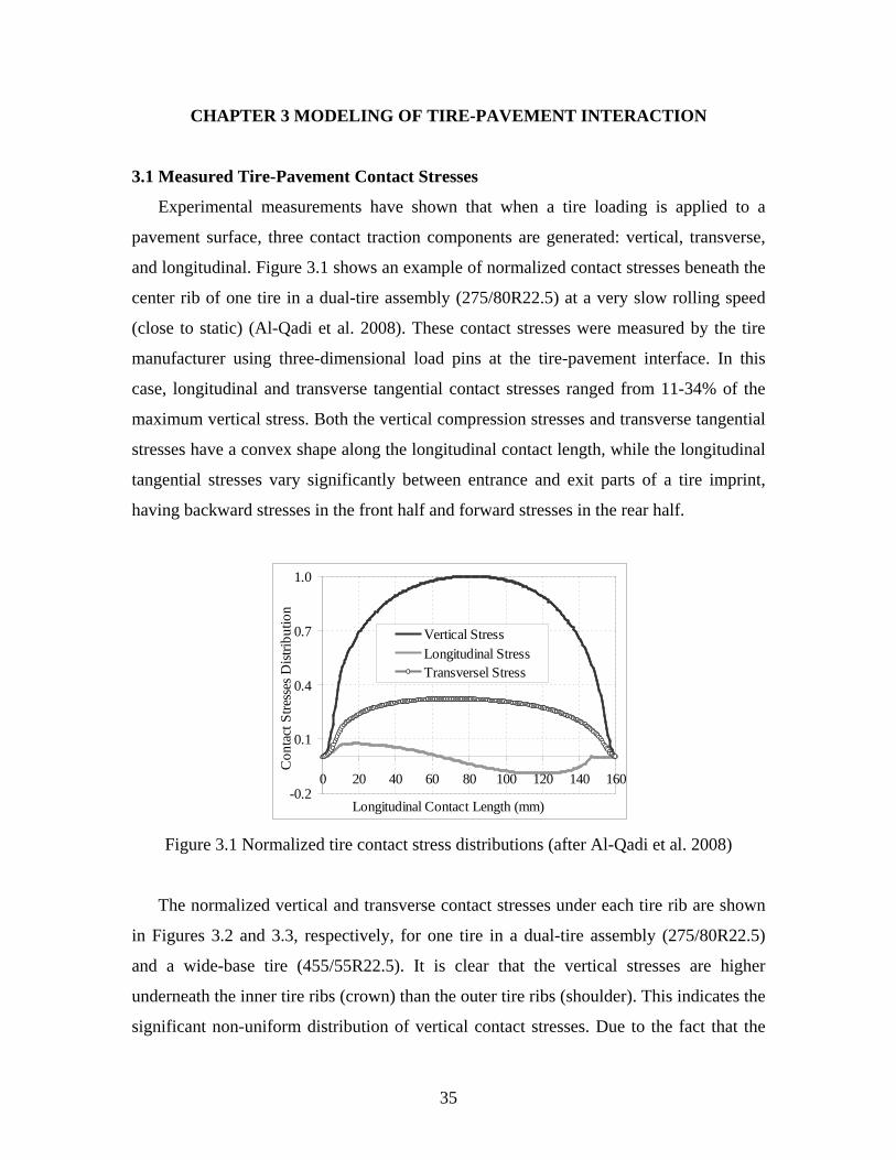
35
CHAPTER 3 MODELING OF TIRE-PAVEMENT INTERACTION
3.1 Measured Tire-Pavement Contact Stresses
Experimental measurements have shown that when a tire loading is applied to a
pavement surface, three contact traction components are generated: vertical, transverse,
and longitudinal. Figure 3.1 shows an example of normalized contact stresses beneath the
center rib of one tire in a dual-tire assembly (275/80R22.5) at a very slow rolling speed
(close to static) (Al-Qadi et al. 2008). These contact stresses were measured by the tire
manufacturer using three-dimensional load pins at the tire-pavement interface. In this
case, longitudinal and transverse tangential contact stresses ranged from 11-34% of the
maximum vertical stress. Both the vertical compression stresses and transverse tangential
stresses have a convex shape along the longitudinal contact length, while the longitudinal
tangential stresses vary significantly between entrance and exit parts of a tire imprint,
having backward stresses in the front half and forward stresses in the rear half.
-0.2
0.1
0.4
0.7
1.0
0 20 40 60 80 100 120 140 160
Longitudinal Contact Length (mm)
Con
tact
Stre
sses
Dist
ribut
ion
Vertical StressLongitudinal StressTransversel Stress
Figure 3.1 Normalized tire contact stress distributions (after Al-Qadi et al. 2008)
The normalized vertical and transverse contact stresses under each tire rib are shown
in Figures 3.2 and 3.3, respectively, for one tire in a dual-tire assembly (275/80R22.5)
and a wide-base tire (455/55R22.5). It is clear that the vertical stresses are higher
underneath the inner tire ribs (crown) than the outer tire ribs (shoulder). This indicates the
significant non-uniform distribution of vertical contact stresses. Due to the fact that the
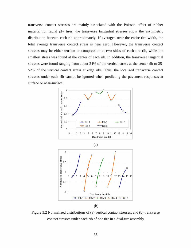
36
transverse contact stresses are mainly associated with the Poisson effect of rubber
material for radial ply tires, the transverse tangential stresses show the asymmetric
distribution beneath each rib approximately. If averaged over the entire tire width, the
total average transverse contact stress is near zero. However, the transverse contact
stresses may be either tension or compression at two sides of each tire rib, while the
smallest stress was found at the center of each rib. In addition, the transverse tangential
stresses were found ranging from about 24% of the vertical stress at the center rib to 35-
52% of the vertical contact stress at edge ribs. Thus, the localized transverse contact
stresses under each rib cannot be ignored when predicting the pavement responses at
surface or near-surface.
0
0.2
0.4
0.6
0.8
1
0 1 2 3 4 5 6 7 8 9 10 11 12 13 14 15 16Data Points in a Rib
Nor
mal
ized
Ver
tical
Con
tact
Stre
ss
Rib 1 Rib 2 Rib 3Rib 4 Rib 5
(a)
-1
-0.5
0
0.5
1
0 1 2 3 4 5 6 7 8 9 10 11 12 13 14 15 16
Data Points in a Rib
Nor
mal
ized
Tra
nsve
rse
Stre
ss
Rib 1 Rib 2 Rib 3 Rib 4 Rib 5
(b)
Figure 3.2 Normalized distributions of (a) vertical contact stresses; and (b) transverse
contact stresses under each rib of one tire in a dual-tire assembly
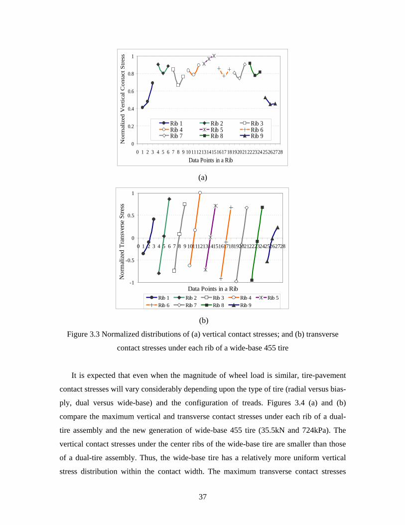
37
0
0.2
0.4
0.6
0.8
1
0 1 2 3 4 5 6 7 8 9 10111213141516171819202122232425262728Data Points in a Rib
Nor
mal
ized
Ver
tical
Con
tact
Stre
ssRib 1 Rib 2 Rib 3Rib 4 Rib 5 Rib 6Rib 7 Rib 8 Rib 9
(a)
-1
-0.5
0
0.5
1
0 1 2 3 4 5 6 7 8 9 10111213141516171819202122232425262728
Data Points in a Rib
Nor
mal
ized
Tra
nsve
rse
Stre
ss
Rib 1 Rib 2 Rib 3 Rib 4 Rib 5Rib 6 Rib 7 Rib 8 Rib 9
(b)
Figure 3.3 Normalized distributions of (a) vertical contact stresses; and (b) transverse
contact stresses under each rib of a wide-base 455 tire
It is expected that even when the magnitude of wheel load is similar, tire-pavement
contact stresses will vary considerably depending upon the type of tire (radial versus bias-
ply, dual versus wide-base) and the configuration of treads. Figures 3.4 (a) and (b)
compare the maximum vertical and transverse contact stresses under each rib of a dual-
tire assembly and the new generation of wide-base 455 tire (35.5kN and 724kPa). The
vertical contact stresses under the center ribs of the wide-base tire are smaller than those
of a dual-tire assembly. Thus, the wide-base tire has a relatively more uniform vertical
stress distribution within the contact width. The maximum transverse contact stresses
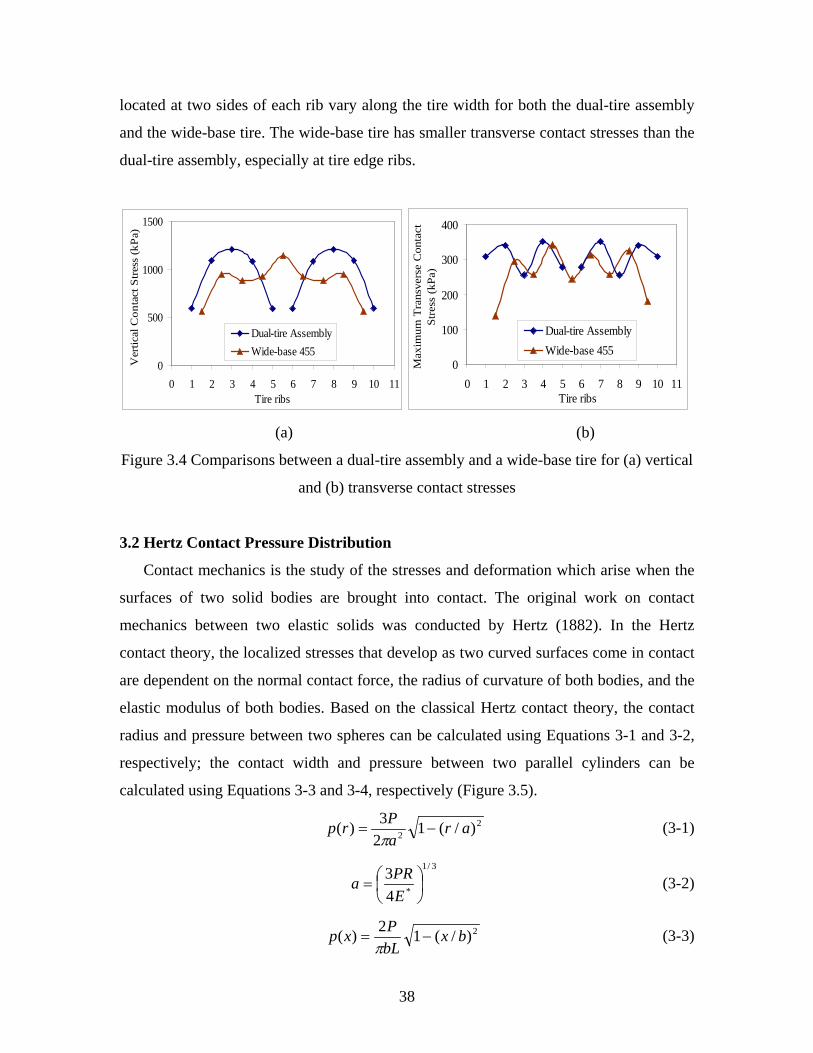
38
located at two sides of each rib vary along the tire width for both the dual-tire assembly
and the wide-base tire. The wide-base tire has smaller transverse contact stresses than the
dual-tire assembly, especially at tire edge ribs.
0
500
1000
1500
0 1 2 3 4 5 6 7 8 9 10 11Tire ribs
Ver
tical
Con
tact
Stre
ss (k
Pa)
Dual-tire AssemblyWide-base 455
0
100
200
300
400
0 1 2 3 4 5 6 7 8 9 10 11Tire ribs
Max
imum
Tra
nsve
rse
Con
tact
Stre
ss (
kPa)
Dual-tire AssemblyWide-base 455
(a) (b)
Figure 3.4 Comparisons between a dual-tire assembly and a wide-base tire for (a) vertical
and (b) transverse contact stresses
3.2 Hertz Contact Pressure Distribution
Contact mechanics is the study of the stresses and deformation which arise when the
surfaces of two solid bodies are brought into contact. The original work on contact
mechanics between two elastic solids was conducted by Hertz (1882). In the Hertz
contact theory, the localized stresses that develop as two curved surfaces come in contact
are dependent on the normal contact force, the radius of curvature of both bodies, and the
elastic modulus of both bodies. Based on the classical Hertz contact theory, the contact
radius and pressure between two spheres can be calculated using Equations 3-1 and 3-2,
respectively; the contact width and pressure between two parallel cylinders can be
calculated using Equations 3-3 and 3-4, respectively (Figure 3.5).
22 )/(1
23)( ar
aPrp −=π
(3-1)
3/1
*43
=
EPRa (3-2)
2)/(12)( bxbLPxp −=
π (3-3)
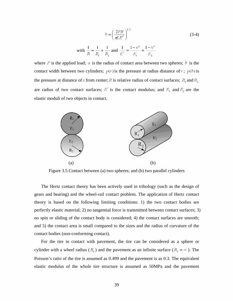
39
(3-4)
with and
where is the applied load; is the radius of contact area between two spheres; is the
contact width between two cylinders; is the pressure at radius distance of ; is
the pressure at distance of from center; is relative radius of contact surfaces; and
are radius of two contact surfaces; is the contact modulus; and and are the
elastic moduli of two objects in contact.
(a) (b)
Figure 3.5 Contact between (a) two spheres; and (b) two parallel cylinders
The Hertz contact theory has been actively used in tribology (such as the design of
gears and bearing) and the wheel-rail contact problem. The application of Hertz contact
theory is based on the following limiting conditions: 1) the two contact bodies are
perfectly elastic material; 2) no tangential force is transmitted between contact surfaces; 3)
no spin or sliding of the contact body is considered; 4) the contact surfaces are smooth;
and 5) the contact area is small compared to the sizes and the radius of curvature of the
contact bodies (non-conforming contact).
For the tire in contact with pavement, the tire can be considered as a sphere or
cylinder with a wheel radius ( ) and the pavement as an infinite surface ( ). The
Poisson’s ratio of the tire is assumed as 0.499 and the pavement is as 0.3. The equivalent
elastic modulus of the whole tire structure is assumed as 50MPa and the pavement
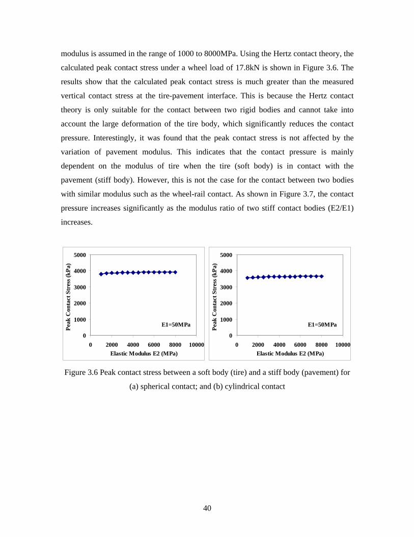
40
modulus is assumed in the range of 1000 to 8000MPa. Using the Hertz contact theory, the
calculated peak contact stress under a wheel load of 17.8kN is shown in Figure 3.6. The
results show that the calculated peak contact stress is much greater than the measured
vertical contact stress at the tire-pavement interface. This is because the Hertz contact
theory is only suitable for the contact between two rigid bodies and cannot take into
account the large deformation of the tire body, which significantly reduces the contact
pressure. Interestingly, it was found that the peak contact stress is not affected by the
variation of pavement modulus. This indicates that the contact pressure is mainly
dependent on the modulus of tire when the tire (soft body) is in contact with the
pavement (stiff body). However, this is not the case for the contact between two bodies
with similar modulus such as the wheel-rail contact. As shown in Figure 3.7, the contact
pressure increases significantly as the modulus ratio of two stiff contact bodies (E2/E1)
increases.
E1=50MPa
0
1000
2000
3000
4000
5000
0 2000 4000 6000 8000 10000Elastic Modulus E2 (MPa)
Peak
Con
tact
Str
ess (
kPa)
E1=50MPa
0
1000
2000
3000
4000
5000
0 2000 4000 6000 8000 10000Elastic Modulus E2 (MPa)
Peak
Con
tact
Str
ess (
kPa)
Figure 3.6 Peak contact stress between a soft body (tire) and a stiff body (pavement) for
(a) spherical contact; and (b) cylindrical contact
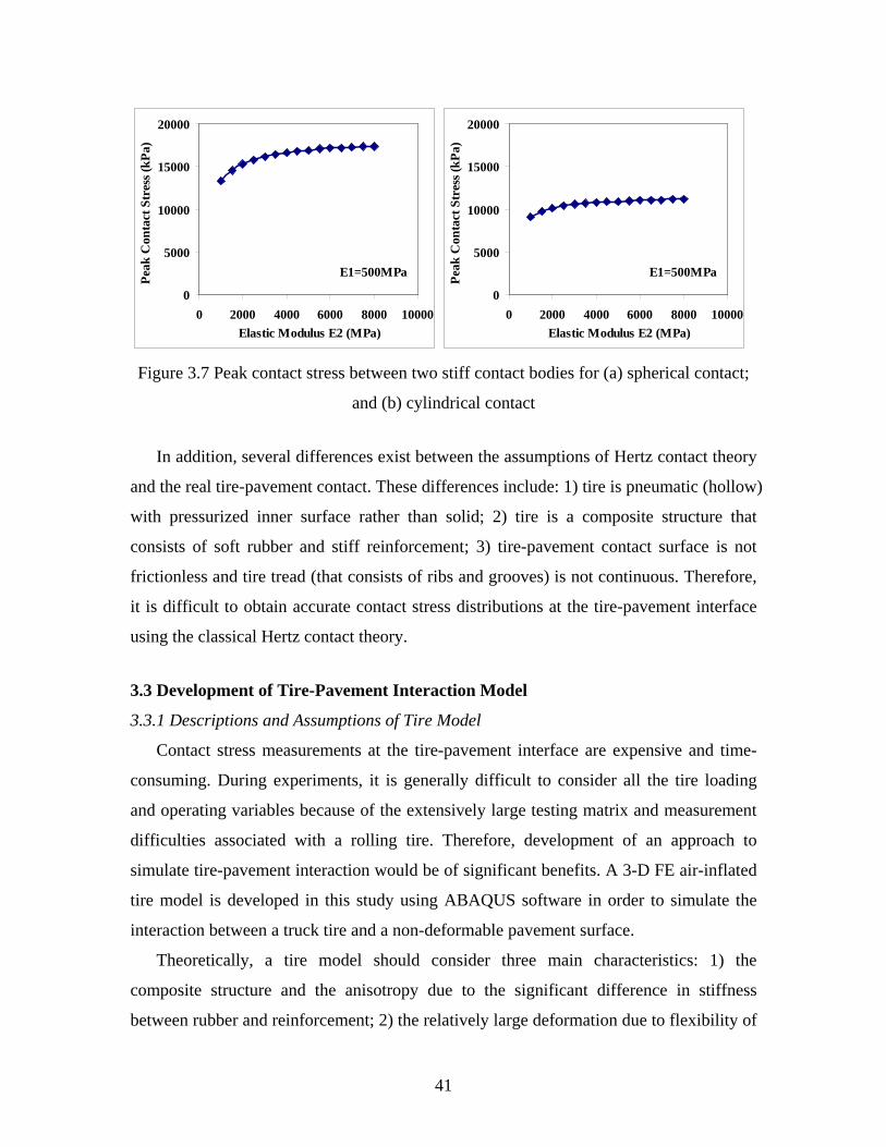
41
E1=500MPa
0
5000
10000
15000
20000
0 2000 4000 6000 8000 10000Elastic Modulus E2 (MPa)
Peak
Con
tact
Str
ess (
kPa)
E1=500MPa
0
5000
10000
15000
20000
0 2000 4000 6000 8000 10000Elastic Modulus E2 (MPa)
Peak
Con
tact
Str
ess (
kPa)
Figure 3.7 Peak contact stress between two stiff contact bodies for (a) spherical contact;
and (b) cylindrical contact
In addition, several differences exist between the assumptions of Hertz contact theory
and the real tire-pavement contact. These differences include: 1) tire is pneumatic (hollow)
with pressurized inner surface rather than solid; 2) tire is a composite structure that
consists of soft rubber and stiff reinforcement; 3) tire-pavement contact surface is not
frictionless and tire tread (that consists of ribs and grooves) is not continuous. Therefore,
it is difficult to obtain accurate contact stress distributions at the tire-pavement interface
using the classical Hertz contact theory.
3.3 Development of Tire-Pavement Interaction Model
3.3.1 Descriptions and Assumptions of Tire Model
Contact stress measurements at the tire-pavement interface are expensive and time-
consuming. During experiments, it is generally difficult to consider all the tire loading
and operating variables because of the extensively large testing matrix and measurement
difficulties associated with a rolling tire. Therefore, development of an approach to
simulate tire-pavement interaction would be of significant benefits. A 3-D FE air-inflated
tire model is developed in this study using ABAQUS software in order to simulate the
interaction between a truck tire and a non-deformable pavement surface.
Theoretically, a tire model should consider three main characteristics: 1) the
composite structure and the anisotropy due to the significant difference in stiffness
between rubber and reinforcement; 2) the relatively large deformation due to flexibility of
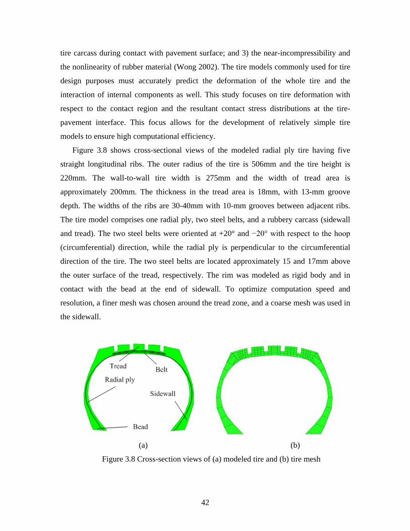
42
tire carcass during contact with pavement surface; and 3) the near-incompressibility and
the nonlinearity of rubber material (Wong 2002). The tire models commonly used for tire
design purposes must accurately predict the deformation of the whole tire and the
interaction of internal components as well. This study focuses on tire deformation with
respect to the contact region and the resultant contact stress distributions at the tire-
pavement interface. This focus allows for the development of relatively simple tire
models to ensure high computational efficiency.
Figure 3.8 shows cross-sectional views of the modeled radial ply tire having five
straight longitudinal ribs. The outer radius of the tire is 506mm and the tire height is
220mm. The wall-to-wall tire width is 275mm and the width of tread area is
approximately 200mm. The thickness in the tread area is 18mm, with 13-mm groove
depth. The widths of the ribs are 30-40mm with 10-mm grooves between adjacent ribs.
The tire model comprises one radial ply, two steel belts, and a rubbery carcass (sidewall
and tread). The two steel belts were oriented at +20° and −20° with respect to the hoop
(circumferential) direction, while the radial ply is perpendicular to the circumferential
direction of the tire. The two steel belts are located approximately 15 and 17mm above
the outer surface of the tread, respectively. The rim was modeled as rigid body and in
contact with the bead at the end of sidewall. To optimize computation speed and
resolution, a finer mesh was chosen around the tread zone, and a coarse mesh was used in
the sidewall.
(a) (b)
Figure 3.8 Cross-section views of (a) modeled tire and (b) tire mesh
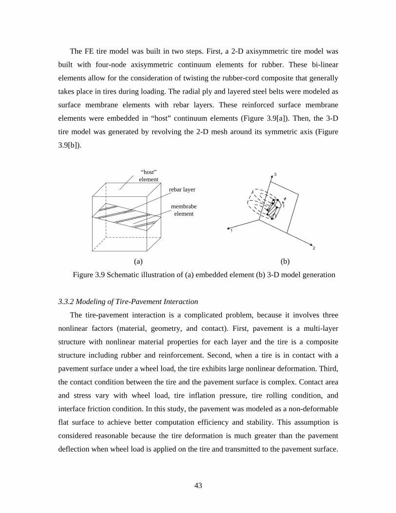
43
The FE tire model was built in two steps. First, a 2-D axisymmetric tire model was
built with four-node axisymmetric continuum elements for rubber. These bi-linear
elements allow for the consideration of twisting the rubber-cord composite that generally
takes place in tires during loading. The radial ply and layered steel belts were modeled as
surface membrane elements with rebar layers. These reinforced surface membrane
elements were embedded in “host” continuum elements (Figure 3.9[a]). Then, the 3-D
tire model was generated by revolving the 2-D mesh around its symmetric axis (Figure
3.9[b]).
“host” element
membrabe element
rebar layer
(a) (b)
Figure 3.9 Schematic illustration of (a) embedded element (b) 3-D model generation
3.3.2 Modeling of Tire-Pavement Interaction
The tire-pavement interaction is a complicated problem, because it involves three
nonlinear factors (material, geometry, and contact). First, pavement is a multi-layer
structure with nonlinear material properties for each layer and the tire is a composite
structure including rubber and reinforcement. Second, when a tire is in contact with a
pavement surface under a wheel load, the tire exhibits large nonlinear deformation. Third,
the contact condition between the tire and the pavement surface is complex. Contact area
and stress vary with wheel load, tire inflation pressure, tire rolling condition, and
interface friction condition. In this study, the pavement was modeled as a non-deformable
flat surface to achieve better computation efficiency and stability. This assumption is
considered reasonable because the tire deformation is much greater than the pavement
deflection when wheel load is applied on the tire and transmitted to the pavement surface.
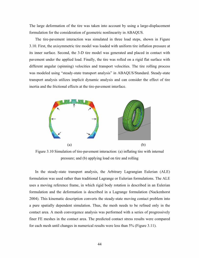
44
The large deformation of the tire was taken into account by using a large-displacement
formulation for the consideration of geometric nonlinearity in ABAQUS.
The tire-pavement interaction was simulated in three load steps, shown in Figure
3.10. First, the axisymmetric tire model was loaded with uniform tire inflation pressure at
its inner surface. Second, the 3-D tire model was generated and placed in contact with
pavement under the applied load. Finally, the tire was rolled on a rigid flat surface with
different angular (spinning) velocities and transport velocities. The tire rolling process
was modeled using “steady-state transport analysis” in ABAQUS/Standard. Steady-state
transport analysis utilizes implicit dynamic analysis and can consider the effect of tire
inertia and the frictional effects at the tire-pavement interface.
(a) (b)
Figure 3.10 Simulation of tire-pavement interaction: (a) inflating tire with internal
pressure; and (b) applying load on tire and rolling
In the steady-state transport analysis, the Arbitrary Lagrangian Eulerian (ALE)
formulation was used rather than traditional Lagrange or Eulerian formulations. The ALE
uses a moving reference frame, in which rigid body rotation is described in an Eulerian
formulation and the deformation is described in a Lagrange formulation (Nackenhorst
2004). This kinematic description converts the steady-state moving contact problem into
a pure spatially dependent simulation. Thus, the mesh needs to be refined only in the
contact area. A mesh convergence analysis was performed with a series of progressively
finer FE meshes in the contact area. The predicted contact stress results were compared
for each mesh until changes in numerical results were less than 5% (Figure 3.11).
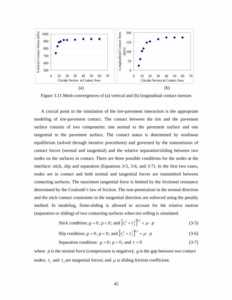
45
500
600
700
800
900
1000
0 10 20 30 40 50 60 70Circular Sectors in Contact Area
Ver
tical
Con
tact
Stre
ss (k
Pa)
0
50
100
150
200
0 10 20 30 40 50 60 70Circular Sectors in Contact Area
Lon
gitu
dina
l Con
tact
Stre
s
(kPa
)
(a) (b)
Figure 3.11 Mesh convergences of (a) vertical and (b) longitudinal contact stresses
A crucial point in the simulation of the tire-pavement interaction is the appropriate
modeling of tire-pavement contact. The contact between the tire and the pavement
surface consists of two components: one normal to the pavement surface and one
tangential to the pavement surface. The contact status is determined by nonlinear
equilibrium (solved through iterative procedures) and governed by the transmission of
contact forces (normal and tangential) and the relative separation/sliding between two
nodes on the surfaces in contact. There are three possible conditions for the nodes at the
interface: stick, slip and separation (Equations 3-5, 3-6, and 3-7). In the first two cases,
nodes are in contact and both normal and tangential forces are transmitted between
contacting surfaces. The maximum tangential force is limited by the frictional resistance
determined by the Coulomb’s law of friction. The non-penetration in the normal direction
and the stick contact constraints in the tangential direction are enforced using the penalty
method. In modeling, finite-sliding is allowed to account for the relative motion
(separation or sliding) of two contacting surfaces when tire rolling is simulated.
Stick condition: 0=g ; 0<p ; and [ ] p⋅<+ µττ5.02
221 (3-5)
Slip condition: 0=g ; 0<p ; and [ ] p⋅=+ µττ5.02
221 (3-6)
Separation condition: 0>g ; 0=p ; and 0=τ (3-7)
where p is the normal force (compression is negative); g is the gap between two contact
nodes; 1τ and 2τ are tangential forces; and µ is sliding friction coefficient.
46
ABAQUS/Standard requires the definition of the contact pair (e.g. the master and
slave surfaces). The master surface is usually the more rigid surface between two contact
surfaces. As default, the slave surface has finer meshes and the nodes of the slave surface
are prohibited from penetrating the element boundaries of the master surface. Two
discretization approaches are available in contact modeling: node-to-surface and surface-
to-surface. The node-to-surface contact prevents any penetration of slave nodes into the
master surface. The surface-to-surface contact enforces the constraints in an average
sense over finite regions of the slave surface. As the mesh is refined, the discrepancies
between the two methods decrease. For a given mesh refinement, the surface-to-surface
approach tends to provide more accurate stresses. In addition, node-to-surface contact
tends to be less costly per iteration than surface-to-surface contact; while finite-sliding
contact tends to converge easily with surface-to-surface contact. Thus, the surface-to-
surface contact is used in this study and the non-deformable pavement surface is defined
as the master surface.
3.3.3 Material Properties
Rubber is a near-incompressible and hyperelastic material with slight viscoelastic
behavior. However, tire manufacturers usually do not reveal information on material
properties of the tire structure. This study focuses on the contact patch shape and stress
distribution at the tire-pavement interface rather than the internal stresses in the tire
structure. Hence, the rubber was assumed as linear elastic material with a Poisson’s ratio
close to 0.5. Different parts of rubber elements (sidewall, shoulder, belt rubber, and tread)
were modeled having variable elastic stiffness. The reinforcements (radial ply and steel
belts) were modeled as a linear elastic material.
Tire load-deflection curves from experimental measurements were used to calibrate
the tire model parameters in this study. The initial elastic modulus of each tire component
was based on tire models in the literature (Zhang 2001; Ghoreishy et al. 2007). The
elastic properties of rubber and reinforcements were then adjusted to obtain deflection
values close to experimental measurements provided by tire manufacturers. Sensitivity
analysis showed that tire deflection is primarily affected by sidewall stiffness and the
orientation of steel belts (crown angles). Good agreements were achieved between the
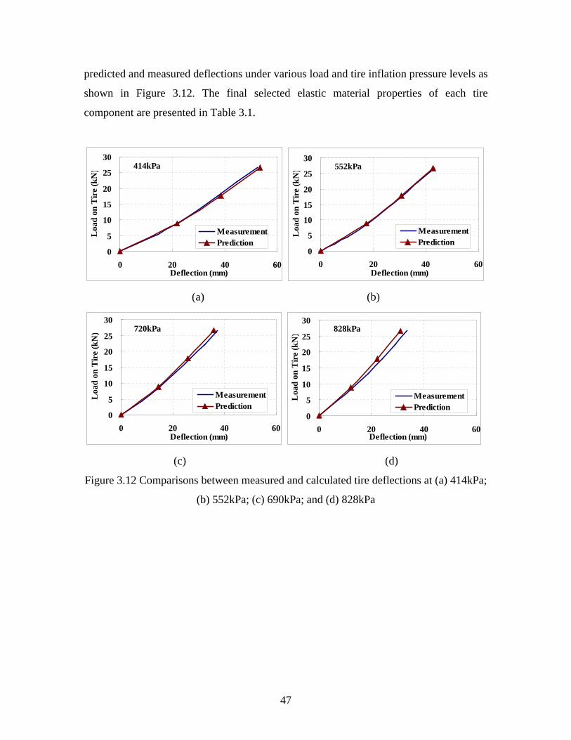
47
predicted and measured deflections under various load and tire inflation pressure levels as
shown in Figure 3.12. The final selected elastic material properties of each tire
component are presented in Table 3.1.
414kPa
0
5
10
15
20
25
30
0 20 40 60Deflection (mm)
Loa
d on
Tir
e (k
N)
MeasurementPrediction
552kPa
0
5
10
15
20
25
30
0 20 40 60Deflection (mm)
Loa
d on
Tir
e (k
N)
MeasurementPrediction
(a) (b)
720kPa
0
5
10
15
20
25
30
0 20 40 60Deflection (mm)
Loa
d on
Tir
e (k
N)
MeasurementPrediction
828kPa
0
5
10
15
20
25
30
0 20 40 60Deflection (mm)
Loa
d on
Tir
e (k
N)
MeasurementPrediction
(c) (d)
Figure 3.12 Comparisons between measured and calculated tire deflections at (a) 414kPa;
(b) 552kPa; (c) 690kPa; and (d) 828kPa
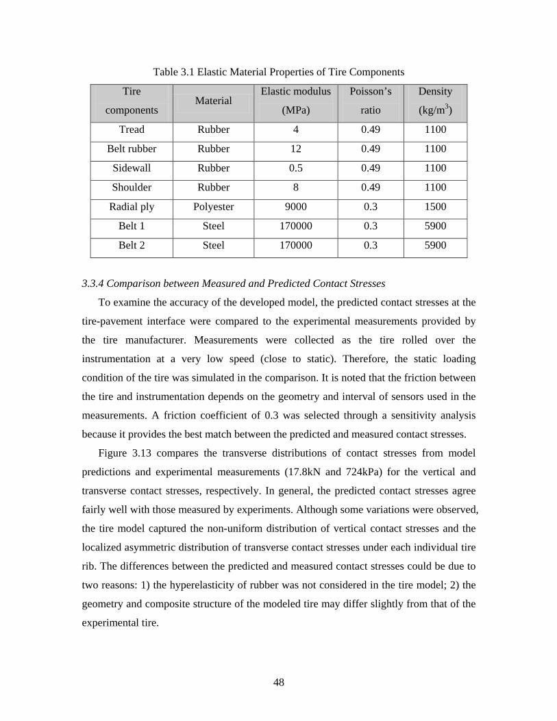
48
Table 3.1 Elastic Material Properties of Tire Components
Tire
components Material
Elastic modulus
(MPa)
Poisson’s
ratio
Density
(kg/m3)
Tread Rubber 4 0.49 1100
Belt rubber Rubber 12 0.49 1100
Sidewall Rubber 0.5 0.49 1100
Shoulder Rubber 8 0.49 1100
Radial ply Polyester 9000 0.3 1500
Belt 1 Steel 170000 0.3 5900
Belt 2 Steel 170000 0.3 5900
3.3.4 Comparison between Measured and Predicted Contact Stresses
To examine the accuracy of the developed model, the predicted contact stresses at the
tire-pavement interface were compared to the experimental measurements provided by
the tire manufacturer. Measurements were collected as the tire rolled over the
instrumentation at a very low speed (close to static). Therefore, the static loading
condition of the tire was simulated in the comparison. It is noted that the friction between
the tire and instrumentation depends on the geometry and interval of sensors used in the
measurements. A friction coefficient of 0.3 was selected through a sensitivity analysis
because it provides the best match between the predicted and measured contact stresses.
Figure 3.13 compares the transverse distributions of contact stresses from model
predictions and experimental measurements (17.8kN and 724kPa) for the vertical and
transverse contact stresses, respectively. In general, the predicted contact stresses agree
fairly well with those measured by experiments. Although some variations were observed,
the tire model captured the non-uniform distribution of vertical contact stresses and the
localized asymmetric distribution of transverse contact stresses under each individual tire
rib. The differences between the predicted and measured contact stresses could be due to
two reasons: 1) the hyperelasticity of rubber was not considered in the tire model; 2) the
geometry and composite structure of the modeled tire may differ slightly from that of the
experimental tire.
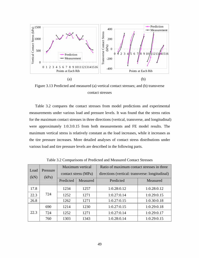
49
0
500
1000
1500
0 1 2 3 4 5 6 7 8 9 10111213141516Points at Each Rib
Ver
tical
Con
tact
Stre
ss (k
Pa)
PredictionMeasurement
-400
-200
0
200
400
0 1 2 3 4 5 6 7 8 9 10111213141516
Points at Each Rib
Tran
sver
se C
onta
ct S
tress
(k
Pa)
PredictionMeasurement
(a) (b)
Figure 3.13 Predicted and measured (a) vertical contact stresses; and (b) transverse
contact stresses
Table 3.2 compares the contact stresses from model predictions and experimental
measurements under various load and pressure levels. It was found that the stress ratios
for the maximum contact stresses in three directions (vertical, transverse, and longitudinal)
were approximately 1:0.3:0.15 from both measurements and FE model results. The
maximum vertical stress is relatively constant as the load increases, while it increases as
the tire pressure increases. More detailed analyses of contact stress distributions under
various load and tire pressure levels are described in the following parts.
Table 3.2 Comparisons of Predicted and Measured Contact Stresses
Load
(kN)
Pressure
(kPa)
Maximum vertical
contact stress (MPa)
Ratio of maximum contact stresses in three
directions (vertical: transverse: longitudinal)
Predicted Measured Predicted Measured
17.8 724
1234 1257 1:0.28:0.12 1:0.28:0.12
22.3 1252 1271 1:0.27:0.14 1:0.29:0.15 26.8 1262 1271 1:0.27:0.15 1:0.30:0.18
22.3 690 1214 1230 1:0.27:0.15 1:0.29:0.18 724 1252 1271 1:0.27:0.14 1:0.29:0.17 760 1303 1343 1:0.28:0.14 1:0.29:0.15
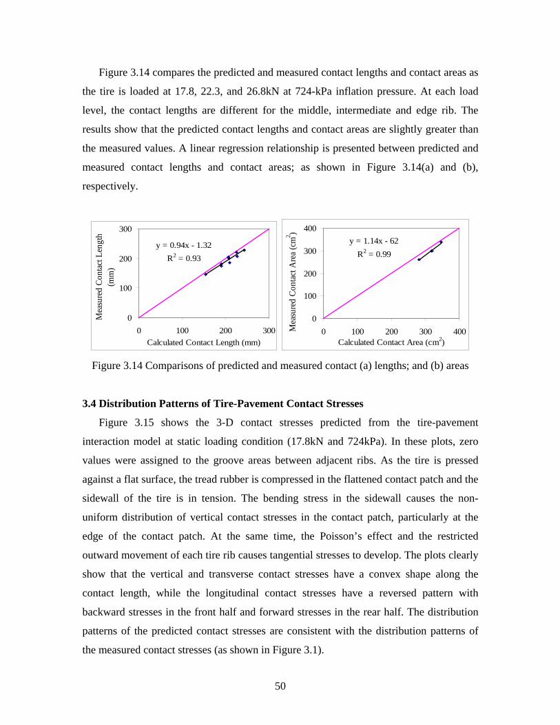
50
Figure 3.14 compares the predicted and measured contact lengths and contact areas as
the tire is loaded at 17.8, 22.3, and 26.8kN at 724-kPa inflation pressure. At each load
level, the contact lengths are different for the middle, intermediate and edge rib. The
results show that the predicted contact lengths and contact areas are slightly greater than
the measured values. A linear regression relationship is presented between predicted and
measured contact lengths and contact areas; as shown in Figure 3.14(a) and (b),
respectively.
y = 0.94x - 1.32R2 = 0.93
0
100
200
300
0 100 200 300Calculated Contact Length (mm)
Mea
sure
d Co
ntac
t Len
gth
(mm
)
y = 1.14x - 62R2 = 0.99
0
100
200
300
400
0 100 200 300 400Calculated Contact Area (cm2)
Mea
sure
d Co
ntac
t Are
a (cm
2 )
Figure 3.14 Comparisons of predicted and measured contact (a) lengths; and (b) areas
3.4 Distribution Patterns of Tire-Pavement Contact Stresses
Figure 3.15 shows the 3-D contact stresses predicted from the tire-pavement
interaction model at static loading condition (17.8kN and 724kPa). In these plots, zero
values were assigned to the groove areas between adjacent ribs. As the tire is pressed
against a flat surface, the tread rubber is compressed in the flattened contact patch and the
sidewall of the tire is in tension. The bending stress in the sidewall causes the non-
uniform distribution of vertical contact stresses in the contact patch, particularly at the
edge of the contact patch. At the same time, the Poisson’s effect and the restricted
outward movement of each tire rib causes tangential stresses to develop. The plots clearly
show that the vertical and transverse contact stresses have a convex shape along the
contact length, while the longitudinal contact stresses have a reversed pattern with
backward stresses in the front half and forward stresses in the rear half. The distribution
patterns of the predicted contact stresses are consistent with the distribution patterns of
the measured contact stresses (as shown in Figure 3.1).
51
Figure 3.16 shows plots of the predicted contact stress distributions along tire contact
length, respectively, for vertical, transverse, and longitudinal contact stress under each rib.
The plots show that the maximum vertical and longitudinal contact stresses are under the
center rib of the tire, while the maximum transverse contact stress is under the
intermediate rib of the tire. It is noted that the transverse contact stress increases in
magnitude with lateral distance from the center of each rib and reaches its maximum at
the edge of each rib (as shown in Figure 3.15(b)). Figure 3.16(b) only shows the
transverse contact stresses beneath one side of the tire rib; it is approximately asymmetric
distribution.
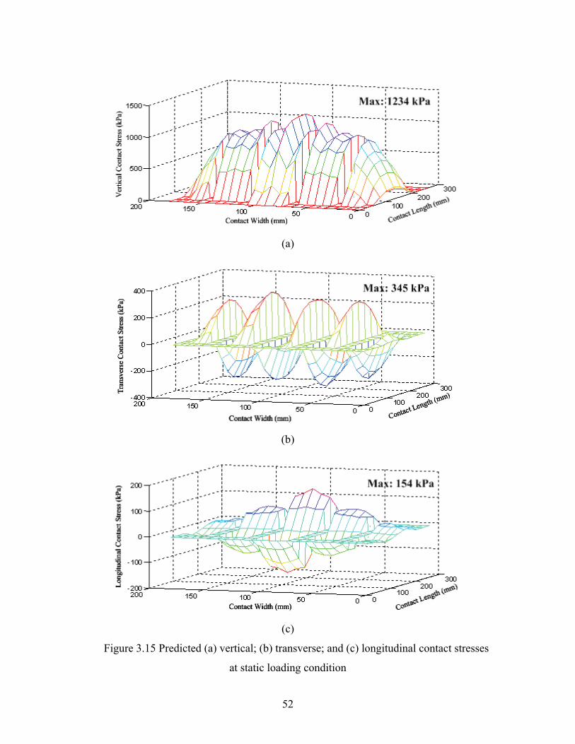
52
(a)
(b)
(c)
Figure 3.15 Predicted (a) vertical; (b) transverse; and (c) longitudinal contact stresses
at static loading condition
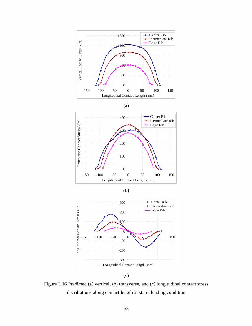
53
0
300
600
900
1200
1500
-150 -100 -50 0 50 100 150Longitudinal Contact Length (mm)
Ver
tical
Cont
act S
tress
(kPa
)
Center RibInermediate RibEdge Rib
(a)
0
100
200
300
400
-150 -100 -50 0 50 100 150Longitudinal Contact Length (mm)
Tran
sver
se C
onta
ct S
tress
(kPa
)
Center RibInermediate RibEdge Rib
(b)
-300
-200
-100
0
100
200
300
-150 -100 -50 0 50 100 150
Longitudinal Contact Length (mm)
Long
itudi
nal C
onta
ct S
tress
(kPa
)
Center RibInermediate RibEdge Rib
(c)
Figure 3.16 Predicted (a) vertical, (b) transverse, and (c) longitudinal contact stress
distributions along contact length at static loading condition
54
Curve fitting techniques were applied to derive a polynomial function to estimate the
interface contact stress distribution as a function of location and peak contact stress. It
was discovered that the convex shape of vertical and transverse contact stress along the
contact patch could be simulated using the elliptic function (Equation 3-8), while the
reverse distribution of longitudinal contact stress from the entrance to the exit along the
contact patch could be simulated using the sinusoid function (Equation 3-9).
2)/(1 Lxqq peak −⋅= (3-8)
)/sin( Lxqq peak ⋅⋅−= π (3-9)
where q is contact stress at location x ( LxL ≤≤− ); peakq is peak contact stress at each
rib along contact length; and L is longitudinal contact length.
3.5 Tire Contact Stresses at Various Load and Tire Inflation Pressure Levels
Figures 3.17 and 3.18 show the distributions of 3-D tire contact stresses, respectively
under high load (40.2kN) and high tire inflation pressure (966kPa). The results show that
as the load increases, the peak contact stress tends to shift towards outer ribs and the
convex shape of the vertical stress tends to flatten in the middle section. This trend likely
occurs due to bending deformation of the sidewall caused by heavy load. This mainly
affects the contact stresses under the outside ribs. As the tire inflation pressure increases,
the stiffness of the whole tire structure increases, especially the central part of the tread
area. Therefore, the vertical contact stress increases the most in the center of the tire
contact area and the stress non-uniformity along the tire contact width becomes more
significant.
The contact length and contact area increases as the load increases but decreases as
the tire inflation pressure increases. It was found that the increase in contact length is
more significant than the increase in contact width due to the relatively high lateral tire
stiffness. The changing trends of tire contact stresses and contact areas as the load or
inflation pressure increases are consistent with the observations from experimental
measurements (De Beer et al. 1997; Douglas et al. 2000; Wang and Al-Qadi 2009).
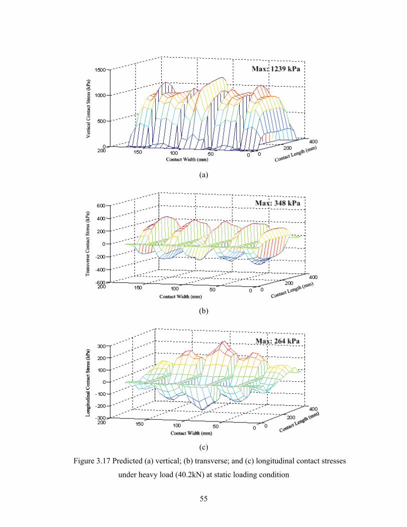
55
(a)
(b)
(c)
Figure 3.17 Predicted (a) vertical; (b) transverse; and (c) longitudinal contact stresses
under heavy load (40.2kN) at static loading condition
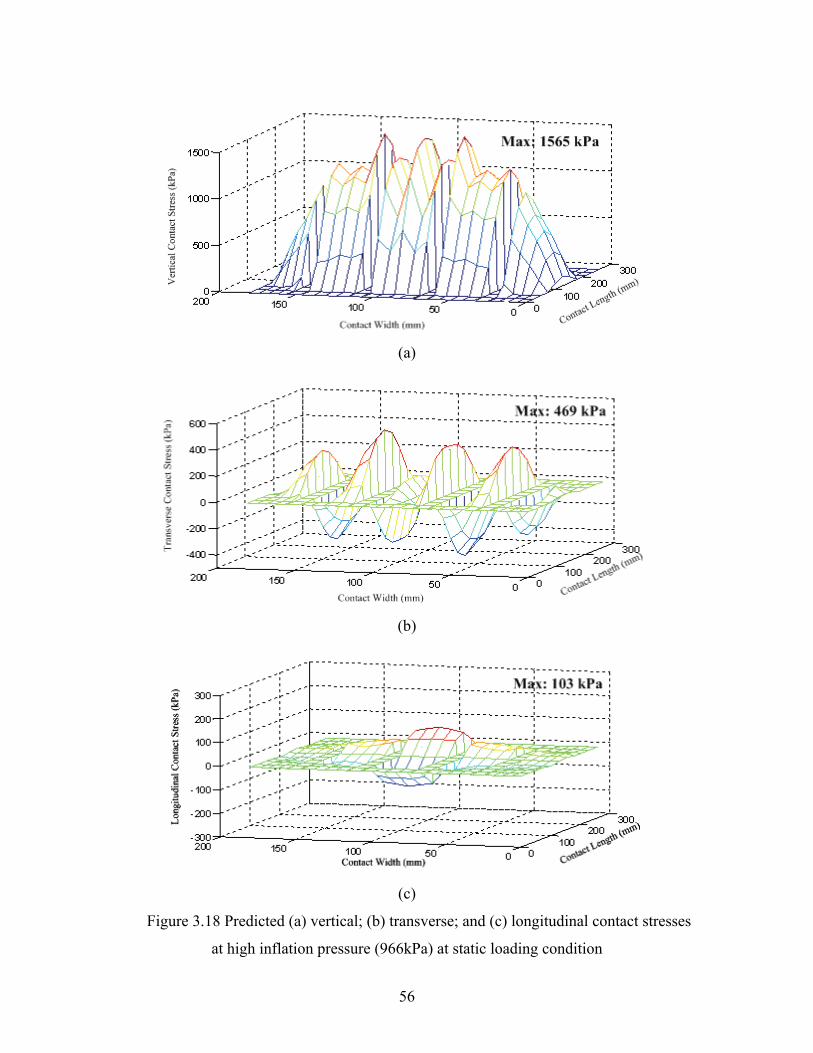
56
(a)
(b)
(c)
Figure 3.18 Predicted (a) vertical; (b) transverse; and (c) longitudinal contact stresses
at high inflation pressure (966kPa) at static loading condition
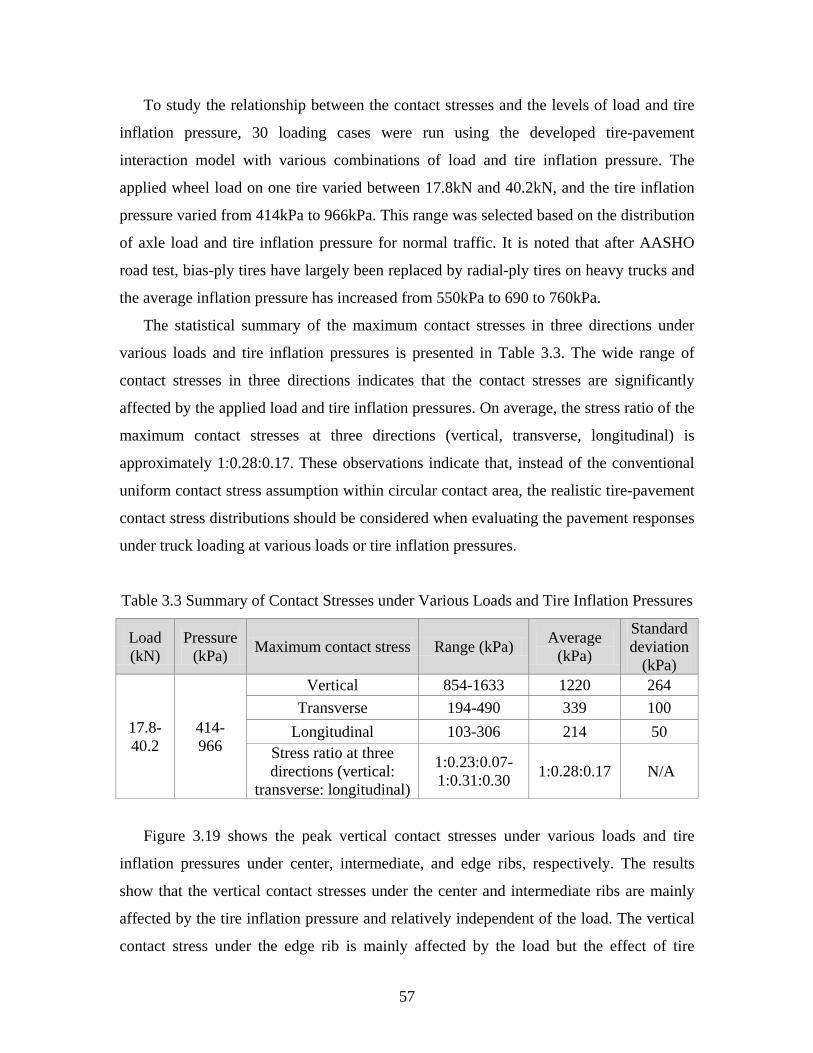
57
To study the relationship between the contact stresses and the levels of load and tire
inflation pressure, 30 loading cases were run using the developed tire-pavement
interaction model with various combinations of load and tire inflation pressure. The
applied wheel load on one tire varied between 17.8kN and 40.2kN, and the tire inflation
pressure varied from 414kPa to 966kPa. This range was selected based on the distribution
of axle load and tire inflation pressure for normal traffic. It is noted that after AASHO
road test, bias-ply tires have largely been replaced by radial-ply tires on heavy trucks and
the average inflation pressure has increased from 550kPa to 690 to 760kPa.
The statistical summary of the maximum contact stresses in three directions under
various loads and tire inflation pressures is presented in Table 3.3. The wide range of
contact stresses in three directions indicates that the contact stresses are significantly
affected by the applied load and tire inflation pressures. On average, the stress ratio of the
maximum contact stresses at three directions (vertical, transverse, longitudinal) is
approximately 1:0.28:0.17. These observations indicate that, instead of the conventional
uniform contact stress assumption within circular contact area, the realistic tire-pavement
contact stress distributions should be considered when evaluating the pavement responses
under truck loading at various loads or tire inflation pressures.
Table 3.3 Summary of Contact Stresses under Various Loads and Tire Inflation Pressures
Load (kN)
Pressure (kPa) Maximum contact stress Range (kPa) Average
(kPa)
Standard deviation
(kPa)
17.8- 40.2
414- 966
Vertical 854-1633 1220 264 Transverse 194-490 339 100
Longitudinal 103-306 214 50 Stress ratio at three directions (vertical:
transverse: longitudinal)
1:0.23:0.07- 1:0.31:0.30 1:0.28:0.17 N/A
Figure 3.19 shows the peak vertical contact stresses under various loads and tire
inflation pressures under center, intermediate, and edge ribs, respectively. The results
show that the vertical contact stresses under the center and intermediate ribs are mainly
affected by the tire inflation pressure and relatively independent of the load. The vertical
contact stress under the edge rib is mainly affected by the load but the effect of tire
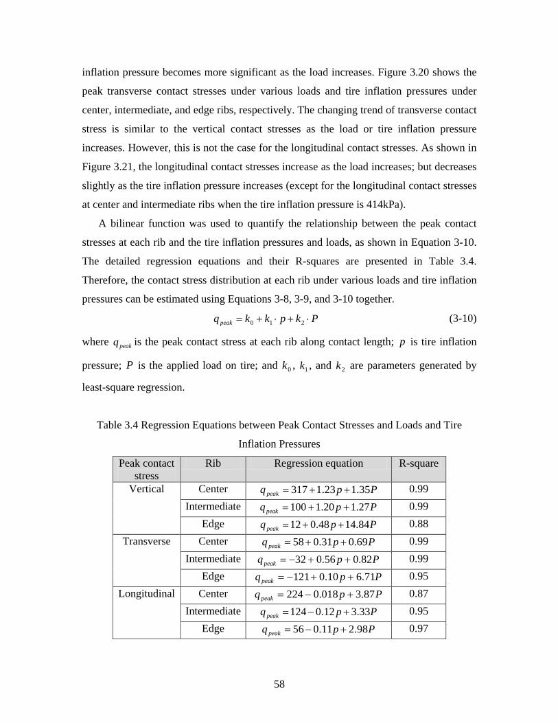
58
inflation pressure becomes more significant as the load increases. Figure 3.20 shows the
peak transverse contact stresses under various loads and tire inflation pressures under
center, intermediate, and edge ribs, respectively. The changing trend of transverse contact
stress is similar to the vertical contact stresses as the load or tire inflation pressure
increases. However, this is not the case for the longitudinal contact stresses. As shown in
Figure 3.21, the longitudinal contact stresses increase as the load increases; but decreases
slightly as the tire inflation pressure increases (except for the longitudinal contact stresses
at center and intermediate ribs when the tire inflation pressure is 414kPa).
A bilinear function was used to quantify the relationship between the peak contact
stresses at each rib and the tire inflation pressures and loads, as shown in Equation 3-10.
The detailed regression equations and their R-squares are presented in Table 3.4.
Therefore, the contact stress distribution at each rib under various loads and tire inflation
pressures can be estimated using Equations 3-8, 3-9, and 3-10 together.
Pkpkkqpeak ⋅+⋅+= 210 (3-10)
where peakq is the peak contact stress at each rib along contact length; p is tire inflation
pressure; P is the applied load on tire; and 0k , 1k , and 2k are parameters generated by
least-square regression.
Table 3.4 Regression Equations between Peak Contact Stresses and Loads and Tire
Inflation Pressures
Peak contact stress
Rib Regression equation R-square
Vertical Center Ppqpeak 35.123.1317 ++= 0.99 Intermediate Ppqpeak 27.120.1100 ++= 0.99
Edge Ppqpeak 84.1448.012 ++= 0.88 Transverse Center Ppqpeak 69.031.058 ++= 0.99
Intermediate Ppqpeak 82.056.032 ++−= 0.99 Edge Ppqpeak 71.610.0121 ++−= 0.95
Longitudinal Center Ppqpeak 87.3018.0224 +−= 0.87 Intermediate Ppqpeak 33.312.0124 +−= 0.95
Edge Ppqpeak 98.211.056 +−= 0.97
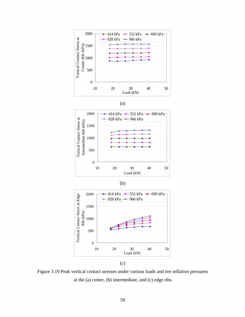
59
0
500
1000
1500
2000
10 20 30 40 50Load (kN)
Ver
tical
Con
tact
Stre
ss a
t C
ente
r Rib
(kPa
)
414 kPa 552 kPa 690 kPa828 kPa 966 kPa
(a)
0
500
1000
1500
2000
10 20 30 40 50Load (kN)
Ver
tical
Con
tact
Stre
ss a
t In
term
edia
te R
ib (k
Pa)
414 kPa 552 kPa 690 kPa828 kPa 966 kPa
(b)
0
500
1000
1500
2000
10 20 30 40 50Load (kN)
Ver
tical
Con
tact
Stre
ss a
t Edg
e R
ib (k
Pa)
414 kPa 552 kPa 690 kPa828 kPa 966 kPa
(c)
Figure 3.19 Peak vertical contact stresses under various loads and tire inflation pressures
at the (a) center, (b) intermediate, and (c) edge ribs
60
0
200
400
600
800
10 20 30 40 50Load (kN)
Tran
sver
se C
onta
ct S
tress
at
Cen
ter R
ib (k
Pa)
414 kPa 552 kPa 690 kPa828 kPa 966 kPa
(a)
0
200
400
600
800
10 20 30 40 50Load (kN)
Tran
sver
se C
onta
ct S
tress
at
Inte
rmed
iate
Rib
(kPa
)
414 kPa 552 kPa 690 kPa828 kPa 966 kPa
(b)
0
200
400
600
800
10 20 30 40 50Load (kN)
Tran
sver
se C
onta
ct S
tress
at
Edge
Rib
(kPa
)
414 kPa 552 kPa 690 kPa828 kPa 966 kPa
(c)
Figure 3.20 Peak transverse contact stresses under various loads and tire inflation
pressures at the (a) center, (b) intermediate, and (c) edge ribs
61
0
200
400
600
10 20 30 40 50Load (kN)
Long
itudi
nal C
onta
ct S
tress
at
Cen
ter R
ib (k
Pa)
414 kPa 552 kPa 690 kPa828 kPa 966 kPa
(a)
0
200
400
600
10 20 30 40 50Load (kN)
Long
itudi
nal C
onta
ct S
tress
at
Inte
rmed
iate
Rib
(kPa
) 414 kPa 552 kPa 690 kPa828 kPa 966 kPa
(b)
0
200
400
600
10 20 30 40 50Load (kN)
Long
itudi
nal C
onta
ct S
tress
at
Edge
Rib
(kPa
)
414 kPa 552 kPa 690 kPa828 kPa 966 kPa
(c)
Figure 3.21 Peak longitudinal contact stresses under various loads and tire inflation
pressures at the (a) center, (b) intermediate, and (c) edge ribs
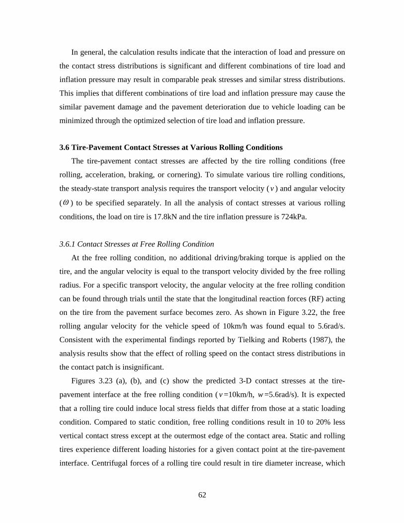
62
In general, the calculation results indicate that the interaction of load and pressure on
the contact stress distributions is significant and different combinations of tire load and
inflation pressure may result in comparable peak stresses and similar stress distributions.
This implies that different combinations of tire load and inflation pressure may cause the
similar pavement damage and the pavement deterioration due to vehicle loading can be
minimized through the optimized selection of tire load and inflation pressure.
3.6 Tire-Pavement Contact Stresses at Various Rolling Conditions
The tire-pavement contact stresses are affected by the tire rolling conditions (free
rolling, acceleration, braking, or cornering). To simulate various tire rolling conditions,
the steady-state transport analysis requires the transport velocity ( v ) and angular velocity
(ω ) to be specified separately. In all the analysis of contact stresses at various rolling
conditions, the load on tire is 17.8kN and the tire inflation pressure is 724kPa.
3.6.1 Contact Stresses at Free Rolling Condition
At the free rolling condition, no additional driving/braking torque is applied on the
tire, and the angular velocity is equal to the transport velocity divided by the free rolling
radius. For a specific transport velocity, the angular velocity at the free rolling condition
can be found through trials until the state that the longitudinal reaction forces (RF) acting
on the tire from the pavement surface becomes zero. As shown in Figure 3.22, the free
rolling angular velocity for the vehicle speed of 10km/h was found equal to 5.6rad/s.
Consistent with the experimental findings reported by Tielking and Roberts (1987), the
analysis results show that the effect of rolling speed on the contact stress distributions in
the contact patch is insignificant.
Figures 3.23 (a), (b), and (c) show the predicted 3-D contact stresses at the tire-
pavement interface at the free rolling condition ( v =10km/h, w =5.6rad/s). It is expected
that a rolling tire could induce local stress fields that differ from those at a static loading
condition. Compared to static condition, free rolling conditions result in 10 to 20% less
vertical contact stress except at the outermost edge of the contact area. Static and rolling
tires experience different loading histories for a given contact point at the tire-pavement
interface. Centrifugal forces of a rolling tire could result in tire diameter increase, which
63
is restricted by the pavement surface. This could cause a vertical “axle lift” and a
decrease in tire-pavement contact stresses. The transverse contact stresses at the free
rolling condition are found to be much lower than those at static condition. As expected,
when a tire is in free rolling condition, the longitudinal contact stresses (frictional forces)
are negligible and therefore the tire has low rolling resistance at the free rolling condition.
This variation in contact stresses due to changes from static to rolling conditions is
similar to the measurements reported by Pottinger (1992). Figure 3.24 shows the
measured vertical, transverse, and longitudinal contact stresses of a static and slow rolling
(75mm/sec) radial tire under 4.9-kN load and 200-kPa inflation pressure. Generally, the
stress distributions at the static and free rolling conditions are similar. As the tire goes
from static to rolling state, the stresses decrease in the middle of the footprint and
increase at the boundaries of the footprint for both the vertical and longitudinal stresses;
while the onset of tire rolling leads to a significant reduction in the transverse contact
stresses.
-6
-4
-2
0
2
4
6
2 3 4 5 6 7 8 9 10
Angular Velocity (rad/s)
Long
itudi
nal R
eact
ion
Forc
e (k
N)
.
Figure 3.22 Longitudinal reaction force at various angular velocities for a specific
transport velocity (10km/h)
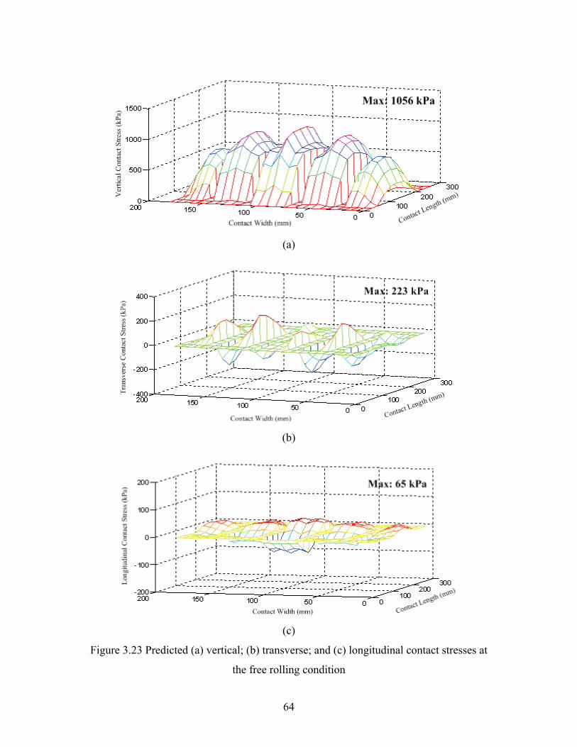
64
(a)
(b)
(c)
Figure 3.23 Predicted (a) vertical; (b) transverse; and (c) longitudinal contact stresses at
the free rolling condition
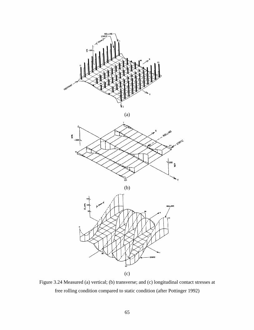
65
(a)
(b)
(c)
Figure 3.24 Measured (a) vertical; (b) transverse; and (c) longitudinal contact stresses at
free rolling condition compared to static condition (after Pottinger 1992)
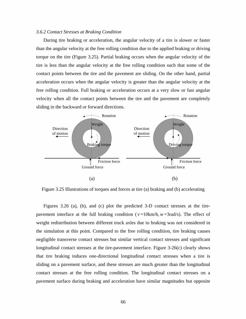
66
3.6.2 Contact Stresses at Braking Condition
During tire braking or acceleration, the angular velocity of a tire is slower or faster
than the angular velocity at the free rolling condition due to the applied braking or driving
torque on the tire (Figure 3.25). Partial braking occurs when the angular velocity of the
tire is less than the angular velocity at the free rolling condition such that some of the
contact points between the tire and the pavement are sliding. On the other hand, partial
acceleration occurs when the angular velocity is greater than the angular velocity at the
free rolling condition. Full braking or acceleration occurs at a very slow or fast angular
velocity when all the contact points between the tire and the pavement are completely
sliding in the backward or forward directions.
Rotation
Friction forceGround force
Braking torque
WeightDirection of motion
Rotation
Friction forceGround force
Driving torque
WeightDirection of motion
(a) (b)
Figure 3.25 Illustrations of torques and forces at tire (a) braking and (b) accelerating
Figures 3.26 (a), (b), and (c) plot the predicted 3-D contact stresses at the tire-
pavement interface at the full braking condition ( v =10km/h, w =3rad/s). The effect of
weight redistribution between different truck axles due to braking was not considered in
the simulation at this point. Compared to the free rolling condition, tire braking causes
negligible transverse contact stresses but similar vertical contact stresses and significant
longitudinal contact stresses at the tire-pavement interface. Figure 3-26(c) clearly shows
that tire braking induces one-directional longitudinal contact stresses when a tire is
sliding on a pavement surface, and these stresses are much greater than the longitudinal
contact stresses at the free rolling condition. The longitudinal contact stresses on a
pavement surface during braking and acceleration have similar magnitudes but opposite
67
directions with forward stresses at braking and backward stresses at acceleration. These
longitudinal contact stresses may lead to severe pavement deterioration, such as
shoving/corrugation and slippage cracking; especially at pavement intersections or
longitudinal sloped pavements.
The level of braking/acceleration can be defined using the slip ratio, as shown in
Equation 3-11 (Henry 2000). The slip ratio represents the locking status of a tire. For
example, the slip ratio is zero when the tire is free rolling and the slip ratio is 100% when
the tire is full braking. Figure 3.27 shows the longitudinal contact stress distributions
along tire contact length due to tire braking at different slip ratios. It shows that the
longitudinal contact stress increases as the slip ratio increases until the peak friction force
is achieved at the full braking condition. For partial braking, the contact patch can be
divided into two regions: a forward “stick” region in the entrance part and an aft “slide”
region in the exit part. In the “slide” region, the longitudinal contact stresses on pavement
surface are approximately equal to the vertical contact stresses multiplied by the friction
coefficient. It indicates that as the tire is sliding at high slip ratios, the longitudinal
contact stresses can be estimated from the vertical contact stresses and the pavement
surface friction coefficient.
Slip ratio = v
rv ⋅−ω (3-11)
where v is the vehicle travel speed ;ω is the angular velocity of the tire; and r is the
rolling radius at the free rolling condition.
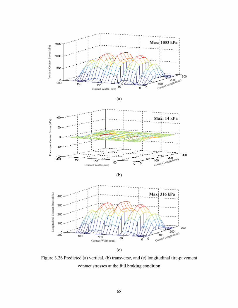
68
(a)
(b)
(c)
Figure 3.26 Predicted (a) vertical, (b) transverse, and (c) longitudinal tire-pavement
contact stresses at the full braking condition
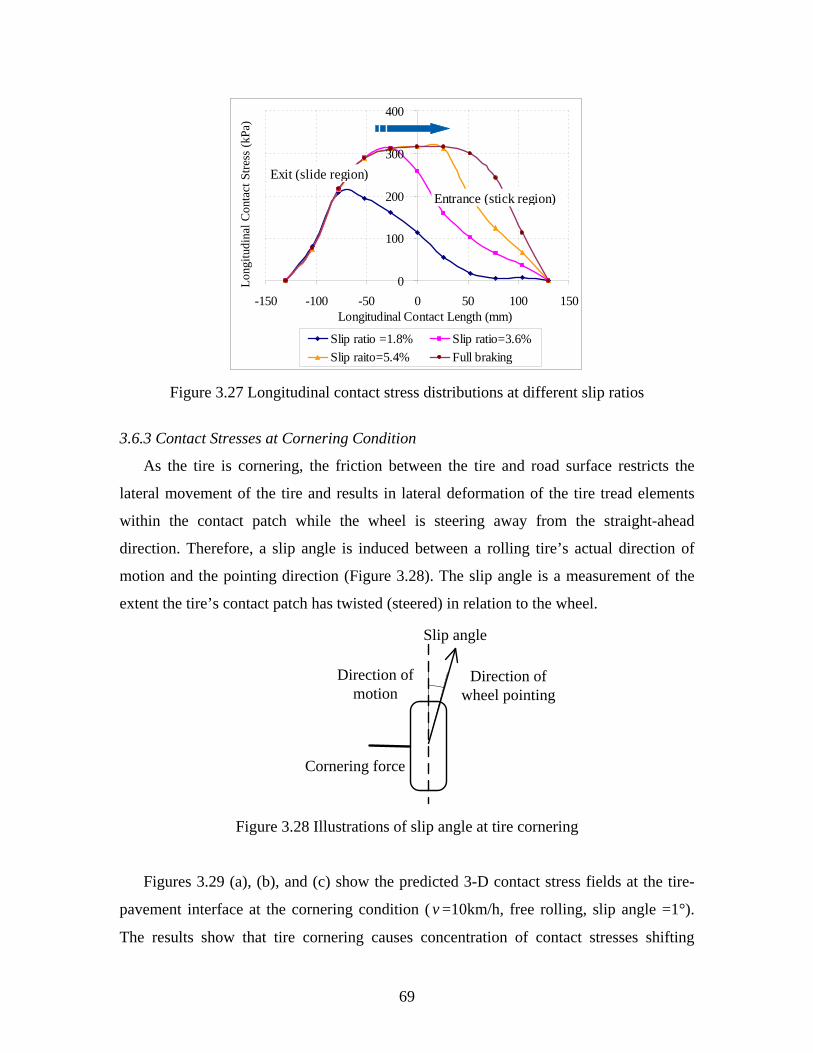
69
0
100
200
300
400
-150 -100 -50 0 50 100 150Longitudinal Contact Length (mm)
Long
itudi
nal C
onta
ct S
tress
(kPa
)
Slip ratio =1.8% Slip ratio=3.6%Slip raito=5.4% Full braking
Exit (slide region)
Entrance (stick region)
Figure 3.27 Longitudinal contact stress distributions at different slip ratios
3.6.3 Contact Stresses at Cornering Condition
As the tire is cornering, the friction between the tire and road surface restricts the
lateral movement of the tire and results in lateral deformation of the tire tread elements
within the contact patch while the wheel is steering away from the straight-ahead
direction. Therefore, a slip angle is induced between a rolling tire’s actual direction of
motion and the pointing direction (Figure 3.28). The slip angle is a measurement of the
extent the tire’s contact patch has twisted (steered) in relation to the wheel.
Direction of wheel pointing
Direction of motion
Slip angle
Cornering force
Figure 3.28 Illustrations of slip angle at tire cornering
Figures 3.29 (a), (b), and (c) show the predicted 3-D contact stress fields at the tire-
pavement interface at the cornering condition ( v =10km/h, free rolling, slip angle =1°).
The results show that tire cornering causes concentration of contact stresses shifting
70
toward to the right side of the contact patch, which lies on the inner side of the right turn.
This indicates that the right tire shoulder is more compressed to the road surface than the
left one during cornering. Hence, the contact stress distribution is no longer symmetric
with respect to the center plane and the contact patch at the right side is longer than the
one at the left side. Similar to the free rolling condition, the longitudinal contact stresses
at the tire cornering condition are negligible. However, tire cornering causes greater
vertical and transverse contact stresses compared to the free rolling condition; the peak
contact stresses are concentrated locally at the edge of tire ribs. Localized contact stress
concentration at tire cornering could be affected by the tread pattern of the tire (such as
tread depth, tread profile, arrangement of ribs and grooves, etc).
Figures 3.30 (a) and (b) show the variation of maximum contact stresses with the slip
angle at the cornering condition, respectively, for the vertical and transverse contact
stresses. As the slip angle increases, the maximum contact stresses increase until the slip
angle reaches 5° and then becomes relatively constant. It was found that the localized
stress concentration became more significant as the slip angle increased. The relatively
high vertical and transverse contact stresses at tire cornering could explain the accelerated
pavement deterioration at the curved road sections where frequent vehicle turns occur. In
addition, the high tangential contact stresses generated during vehicle turns would
accelerate the polishing of surface aggregate and reduce surface friction.
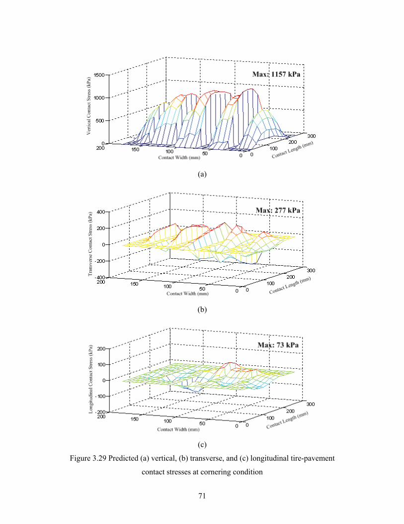
71
(a)
(b)
(c)
Figure 3.29 Predicted (a) vertical, (b) transverse, and (c) longitudinal tire-pavement
contact stresses at cornering condition
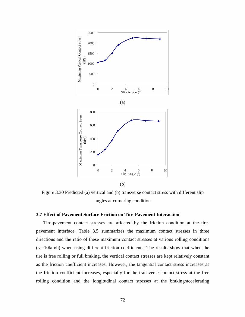
72
0
500
1000
1500
2000
2500
0 2 4 6 8 10Slip Angle (o)
Max
imum
Ver
tical
Con
tact
Stre
s
(kPa
)
(a)
0
200
400
600
800
0 2 4 6 8 10Slip Angle (o)
Max
imum
Tra
nsve
rse
Con
tact
Stre
ss
(kPa
)
(b)
Figure 3.30 Predicted (a) vertical and (b) transverse contact stress with different slip
angles at cornering condition
3.7 Effect of Pavement Surface Friction on Tire-Pavement Interaction
Tire-pavement contact stresses are affected by the friction condition at the tire-
pavement interface. Table 3.5 summarizes the maximum contact stresses in three
directions and the ratio of these maximum contact stresses at various rolling conditions
( v =10km/h) when using different friction coefficients. The results show that when the
tire is free rolling or full braking, the vertical contact stresses are kept relatively constant
as the friction coefficient increases. However, the tangential contact stress increases as
the friction coefficient increases, especially for the transverse contact stress at the free
rolling condition and the longitudinal contact stresses at the braking/accelerating
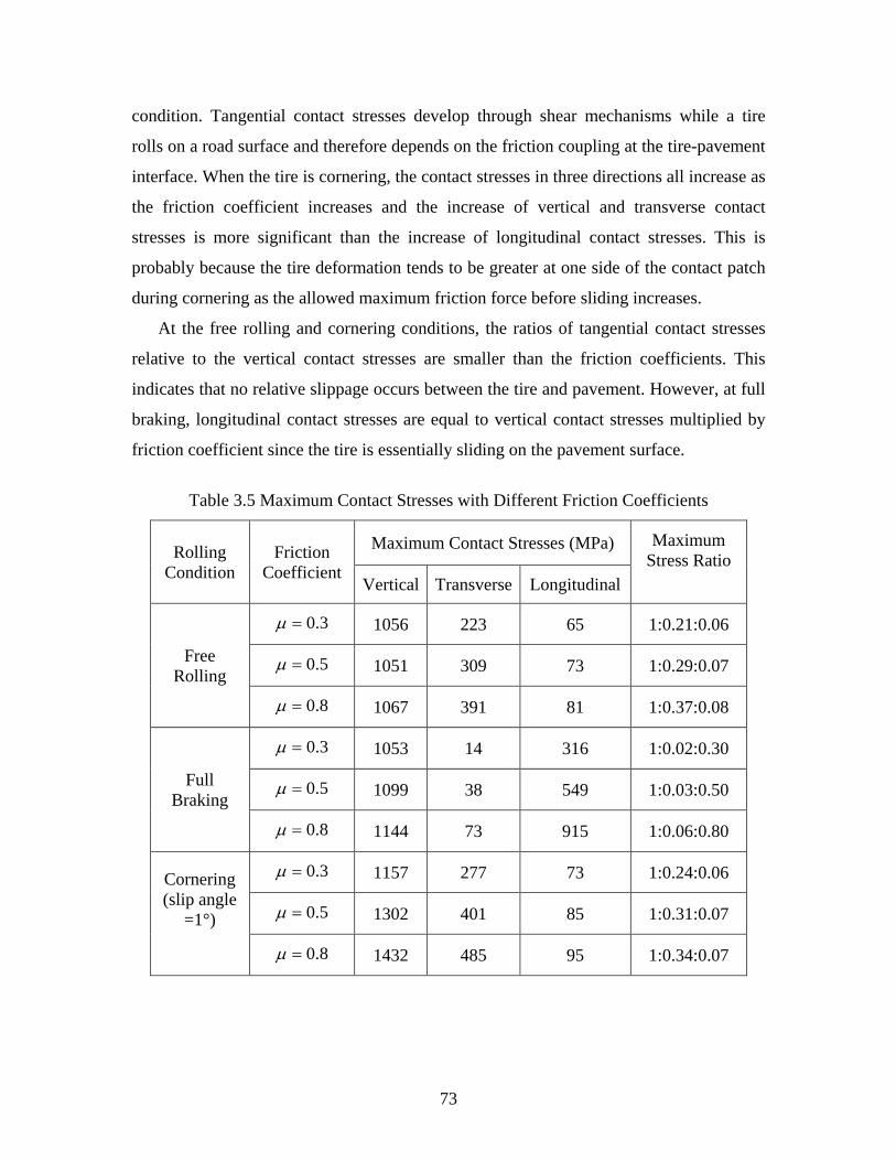
73
condition. Tangential contact stresses develop through shear mechanisms while a tire
rolls on a road surface and therefore depends on the friction coupling at the tire-pavement
interface. When the tire is cornering, the contact stresses in three directions all increase as
the friction coefficient increases and the increase of vertical and transverse contact
stresses is more significant than the increase of longitudinal contact stresses. This is
probably because the tire deformation tends to be greater at one side of the contact patch
during cornering as the allowed maximum friction force before sliding increases.
At the free rolling and cornering conditions, the ratios of tangential contact stresses
relative to the vertical contact stresses are smaller than the friction coefficients. This
indicates that no relative slippage occurs between the tire and pavement. However, at full
braking, longitudinal contact stresses are equal to vertical contact stresses multiplied by
friction coefficient since the tire is essentially sliding on the pavement surface.
Table 3.5 Maximum Contact Stresses with Different Friction Coefficients
Rolling Condition
Friction Coefficient
Maximum Contact Stresses (MPa) Maximum Stress Ratio
Vertical Transverse Longitudinal
Free Rolling
3.0=µ 1056 223 65 1:0.21:0.06
5.0=µ 1051 309 73 1:0.29:0.07
8.0=µ 1067 391 81 1:0.37:0.08
Full Braking
3.0=µ 1053 14 316 1:0.02:0.30
5.0=µ 1099 38 549 1:0.03:0.50
8.0=µ 1144 73 915 1:0.06:0.80
Cornering (slip angle
=1°)
3.0=µ 1157 277 73 1:0.24:0.06
5.0=µ 1302 401 85 1:0.31:0.07
8.0=µ 1432 485 95 1:0.34:0.07
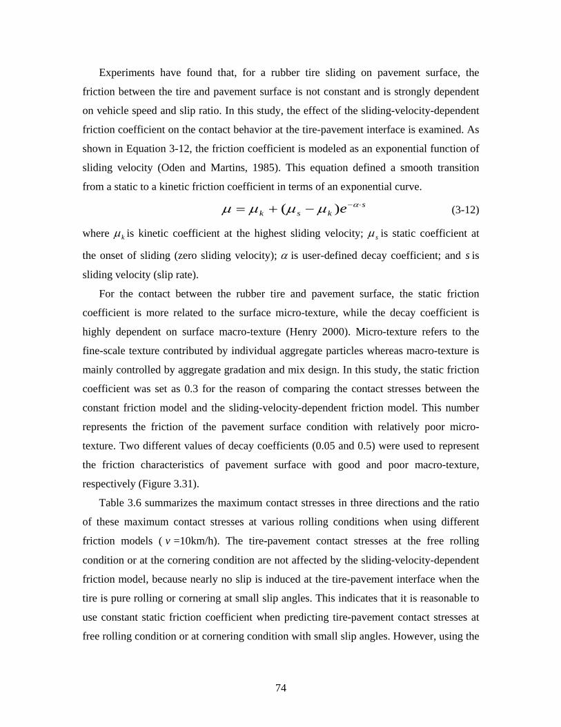
74
Experiments have found that, for a rubber tire sliding on pavement surface, the
friction between the tire and pavement surface is not constant and is strongly dependent
on vehicle speed and slip ratio. In this study, the effect of the sliding-velocity-dependent
friction coefficient on the contact behavior at the tire-pavement interface is examined. As
shown in Equation 3-12, the friction coefficient is modeled as an exponential function of
sliding velocity (Oden and Martins, 1985). This equation defined a smooth transition
from a static to a kinetic friction coefficient in terms of an exponential curve. s
ksk e ⋅−−+= αµµµµ )( (3-12)
where kµ is kinetic coefficient at the highest sliding velocity; sµ is static coefficient at
the onset of sliding (zero sliding velocity); α is user-defined decay coefficient; and s is
sliding velocity (slip rate).
For the contact between the rubber tire and pavement surface, the static friction
coefficient is more related to the surface micro-texture, while the decay coefficient is
highly dependent on surface macro-texture (Henry 2000). Micro-texture refers to the
fine-scale texture contributed by individual aggregate particles whereas macro-texture is
mainly controlled by aggregate gradation and mix design. In this study, the static friction
coefficient was set as 0.3 for the reason of comparing the contact stresses between the
constant friction model and the sliding-velocity-dependent friction model. This number
represents the friction of the pavement surface condition with relatively poor micro-
texture. Two different values of decay coefficients (0.05 and 0.5) were used to represent
the friction characteristics of pavement surface with good and poor macro-texture,
respectively (Figure 3.31).
Table 3.6 summarizes the maximum contact stresses in three directions and the ratio
of these maximum contact stresses at various rolling conditions when using different
friction models ( v =10km/h). The tire-pavement contact stresses at the free rolling
condition or at the cornering condition are not affected by the sliding-velocity-dependent
friction model, because nearly no slip is induced at the tire-pavement interface when the
tire is pure rolling or cornering at small slip angles. This indicates that it is reasonable to
use constant static friction coefficient when predicting tire-pavement contact stresses at
free rolling condition or at cornering condition with small slip angles. However, using the
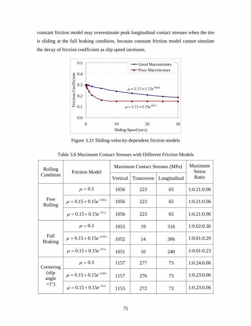
75
constant friction model may overestimate peak longitudinal contact stresses when the tire
is sliding at the full braking condition, because constant friction model cannot simulate
the decay of friction coefficient as slip speed increases.
0.0
0.1
0.2
0.3
0.4
0.5
0 10 20 30Sliding Speed (m/s)
Fric
tion
Coef
ficie
nt
Good MacrotexturePoor Macrotexture
Figure 3.31 Sliding-velocity-dependent friction models
Table 3.6 Maximum Contact Stresses with Different Friction Models
Rolling Condition Friction Model
Maximum Contact Stresses (MPa) Maximum Stress Ratio Vertical Transverse Longitudinal
Free Rolling
3.0=µ 1056 223 65 1:0.21:0.06
se 05.015.015.0 −+=µ 1056 223 65 1:0.21:0.06
se 5.015.015.0 −+=µ 1056 223 65 1:0.21:0.06
Full Braking
3.0=µ 1053 19 316 1:0.02:0.30
se 05.015.015.0 −+=µ 1052 14 306 1:0.01:0.29
se 5.015.015.0 −+=µ 1051 10 240 1:0.01:0.23
Cornering (slip angle =1°)
3.0=µ 1157 277 73 1:0.24:0.06
se 05.015.015.0 −+=µ 1157 276 73 1:0.23:0.06
se 5.015.015.0 −+=µ 1153 272 73 1:0.23:0.06
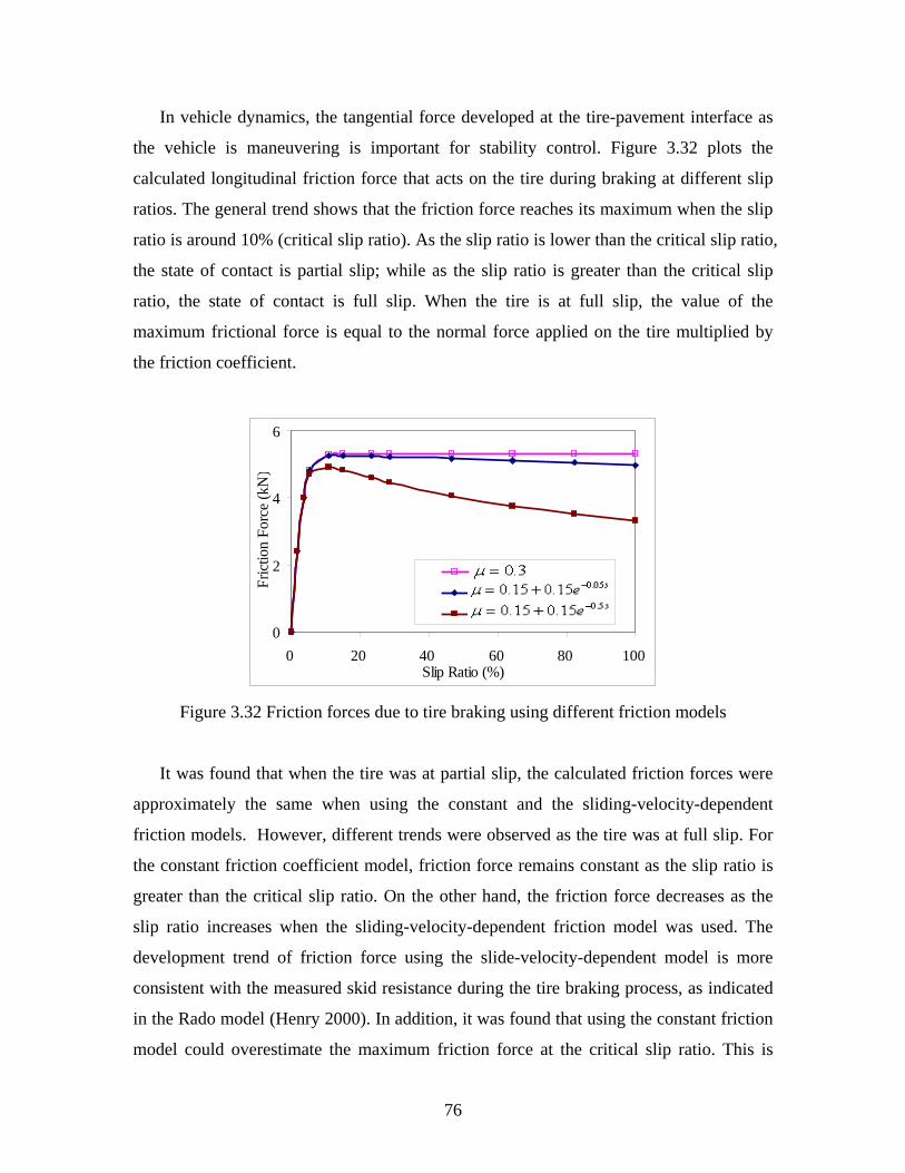
76
In vehicle dynamics, the tangential force developed at the tire-pavement interface as
the vehicle is maneuvering is important for stability control. Figure 3.32 plots the
calculated longitudinal friction force that acts on the tire during braking at different slip
ratios. The general trend shows that the friction force reaches its maximum when the slip
ratio is around 10% (critical slip ratio). As the slip ratio is lower than the critical slip ratio,
the state of contact is partial slip; while as the slip ratio is greater than the critical slip
ratio, the state of contact is full slip. When the tire is at full slip, the value of the
maximum frictional force is equal to the normal force applied on the tire multiplied by
the friction coefficient.
0
2
4
6
0 20 40 60 80 100Slip Ratio (%)
Fric
tion
Forc
e (k
N)
ConstantVarying mu texture 1Varying mu texture 2
Figure 3.32 Friction forces due to tire braking using different friction models
It was found that when the tire was at partial slip, the calculated friction forces were
approximately the same when using the constant and the sliding-velocity-dependent
friction models. However, different trends were observed as the tire was at full slip. For
the constant friction coefficient model, friction force remains constant as the slip ratio is
greater than the critical slip ratio. On the other hand, the friction force decreases as the
slip ratio increases when the sliding-velocity-dependent friction model was used. The
development trend of friction force using the slide-velocity-dependent model is more
consistent with the measured skid resistance during the tire braking process, as indicated
in the Rado model (Henry 2000). In addition, it was found that using the constant friction
model could overestimate the maximum friction force at the critical slip ratio. This is
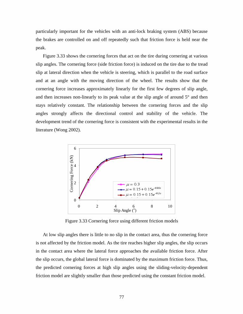
77
particularly important for the vehicles with an anti-lock braking system (ABS) because
the brakes are controlled on and off repeatedly such that friction force is held near the
peak.
Figure 3.33 shows the cornering forces that act on the tire during cornering at various
slip angles. The cornering force (side friction force) is induced on the tire due to the tread
slip at lateral direction when the vehicle is steering, which is parallel to the road surface
and at an angle with the moving direction of the wheel. The results show that the
cornering force increases approximately linearly for the first few degrees of slip angle,
and then increases non-linearly to its peak value at the slip angle of around 5° and then
stays relatively constant. The relationship between the cornering forces and the slip
angles strongly affects the directional control and stability of the vehicle. The
development trend of the cornering force is consistent with the experimental results in the
literature (Wong 2002).
0
2
4
6
0 2 4 6 8 10Slip Angle (o)
Corn
erin
g Fo
rce
(kN
)
ConstantVarying mu texture 1Varying mu texture 2
Figure 3.33 Cornering force using different friction models
At low slip angles there is little to no slip in the contact area, thus the cornering force
is not affected by the friction model. As the tire reaches higher slip angles, the slip occurs
in the contact area where the lateral force approaches the available friction force. After
the slip occurs, the global lateral force is dominated by the maximum friction force. Thus,
the predicted cornering forces at high slip angles using the sliding-velocity-dependent
friction model are slightly smaller than those predicted using the constant friction model.
78
3.8 Summary
In this chapter, an air-inflated 3-D tire model was built and the interaction between a
tire and a non-deformable pavement surface was simulated. The tire was modeled as a
composite structure including rubber and reinforcement. The material parameters of each
tire component were calibrated through the measured tire load-deflection curves. The
steady-state tire rolling process was simulated using an Arbitrary Lagrangian Eulerian
(ALE) formulation. The model results are consistent with measured values and validate
the non-uniformity vertical contact stresses and localized tangential contact stresses at the
tire-pavement interface.
The developed tire-pavement interaction model shows the potential to evaluate the
mechanism of load distribution at the tire-pavement interface under various tire loading
and rolling conditions. The model results show that the load primarily affects the vertical
contact stresses, at the edge of tire contact area, and the longitudinal contact stresses. The
tire inflation pressure, on the other hand, primarily controls the vertical contact stresses,
at the center of tire contact area, and the transverse contact stresses. A statistical model is
developed to predict peak contact stresses at each tire rib under various load and tire
inflation pressure levels. In addition, vehicle maneuvering behavior significantly affects
the magnitudes and distributions of tire-pavement contact stresses. For example, tire
braking/acceleration induces significant longitudinal contact stresses, while tire cornering
causes greater vertical and transverse contact stresses shifting toward one side of the
contact patch. The tire-pavement contact stresses at various tire rolling conditions are
significantly affected by the friction at the tire-pavement interface and vehicle operating
parameters, such as slip ratio and slip angle.
79
CHAPTER 4 FINITE ELEMENT MODELING OF FLEXIBLE PAVEMENT
4.1 Building an FE Model of Flexible Pavement
A 3-D FE model of flexible pavement was simulated using the software ABAQUS.
The 3-D FE model is more appropriate, compared to an axisymmetric or 2-D plane model.
It allows considering 3-D contact stress distributions at the tire-pavement interface and
dynamic transient loading associated with a moving vehicle.
Since the behavior of a layered pavement system may not be approximated using
truss, beam, or shell elements, 3-D continuum solid elements are often used. In this study,
the eight-node, linear brick elements with reduced integration were used in the finite
domains, whereas infinite elements were used to reduce a large number of far-field
elements without significant loss of accuracy and to create a “silent” boundary for the
dynamic analysis (Figure 4.1). The infinite element has a special shape function for the
geometry at the infinite boundary and thus has zero displacement as the coordinate
approaches infinity.
The infinite elements provided in ABAQUS introduce additional normal and shear
tractions (viscous damping boundary) on the FE boundary that are proportional to the
normal and shear components of the velocity of the boundary, as shown in Equations 4-1
and 4-2 (Lysmer and Kuhlemeyer 1969; ABAQUS 2007). This could minimize the
reflection of dilatational and shear wave energy back into the FE mesh and it usually
provides acceptable results for most practical cases.
uc p ⋅⋅= ρσ (4-1)
vcs ⋅⋅= ρτ (4-2)
with ρνν
ν)1)(21(
)1(+−
−=
Ecp and ρν )1(2 +
=Ecs
where σ and τ are normal and shear stresses along the finite/infinite elements border,
respectively; ρ is material density; pc and sc are longitudinal and shear wave velocities,
respectively; u and v are velocities in the normal and tangential directions, respectively;
E is the modulus of elasticity; and ν is the Poisson’s ratio.
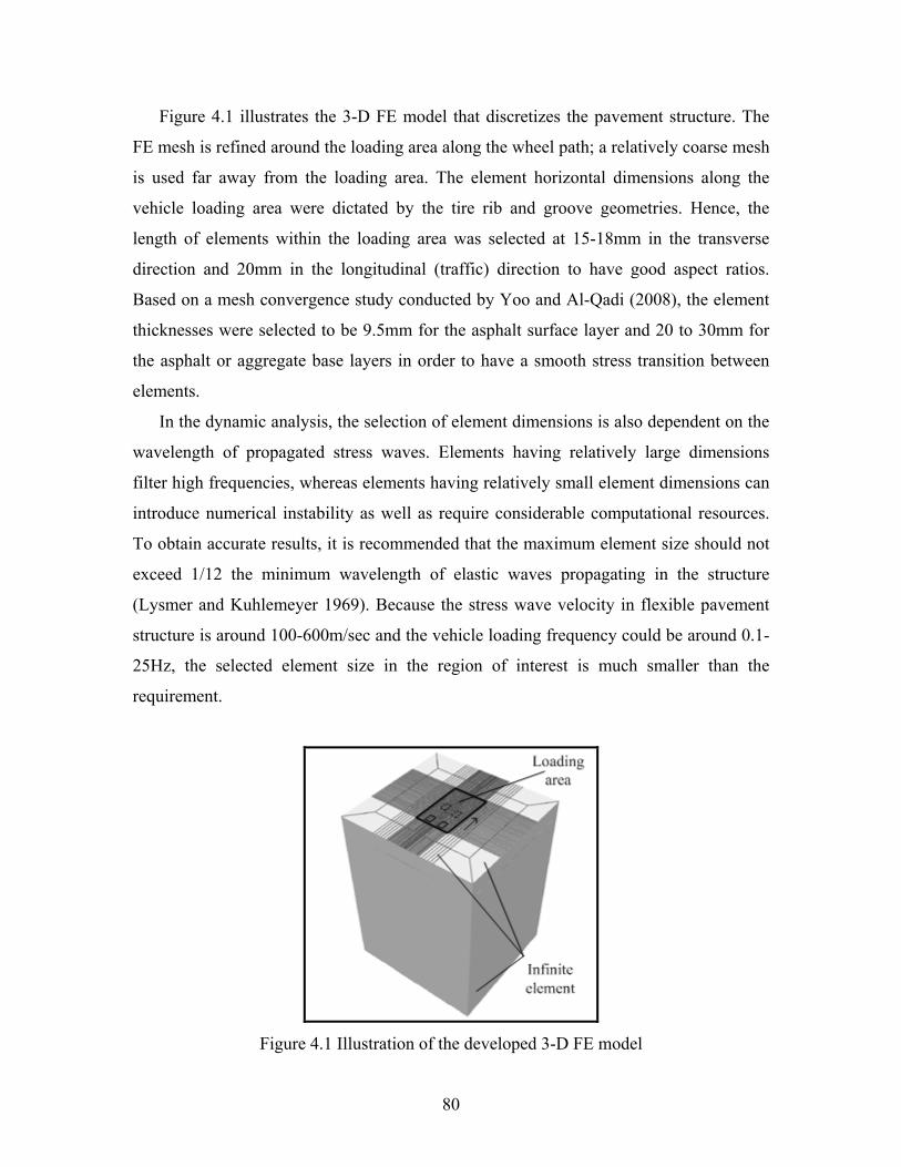
80
Figure 4.1 illustrates the 3-D FE model that discretizes the pavement structure. The
FE mesh is refined around the loading area along the wheel path; a relatively coarse mesh
is used far away from the loading area. The element horizontal dimensions along the
vehicle loading area were dictated by the tire rib and groove geometries. Hence, the
length of elements within the loading area was selected at 15-18mm in the transverse
direction and 20mm in the longitudinal (traffic) direction to have good aspect ratios.
Based on a mesh convergence study conducted by Yoo and Al-Qadi (2008), the element
thicknesses were selected to be 9.5mm for the asphalt surface layer and 20 to 30mm for
the asphalt or aggregate base layers in order to have a smooth stress transition between
elements.
In the dynamic analysis, the selection of element dimensions is also dependent on the
wavelength of propagated stress waves. Elements having relatively large dimensions
filter high frequencies, whereas elements having relatively small element dimensions can
introduce numerical instability as well as require considerable computational resources.
To obtain accurate results, it is recommended that the maximum element size should not
exceed 1/12 the minimum wavelength of elastic waves propagating in the structure
(Lysmer and Kuhlemeyer 1969). Because the stress wave velocity in flexible pavement
structure is around 100-600m/sec and the vehicle loading frequency could be around 0.1-
25Hz, the selected element size in the region of interest is much smaller than the
requirement.
Figure 4.1 Illustration of the developed 3-D FE model
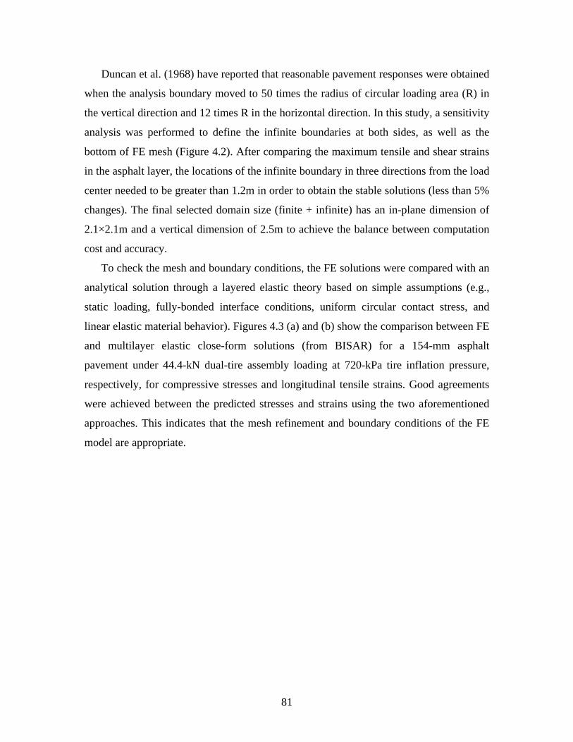
81
Duncan et al. (1968) have reported that reasonable pavement responses were obtained
when the analysis boundary moved to 50 times the radius of circular loading area (R) in
the vertical direction and 12 times R in the horizontal direction. In this study, a sensitivity
analysis was performed to define the infinite boundaries at both sides, as well as the
bottom of FE mesh (Figure 4.2). After comparing the maximum tensile and shear strains
in the asphalt layer, the locations of the infinite boundary in three directions from the load
center needed to be greater than 1.2m in order to obtain the stable solutions (less than 5%
changes). The final selected domain size (finite + infinite) has an in-plane dimension of
2.1×2.1m and a vertical dimension of 2.5m to achieve the balance between computation
cost and accuracy.
To check the mesh and boundary conditions, the FE solutions were compared with an
analytical solution through a layered elastic theory based on simple assumptions (e.g.,
static loading, fully-bonded interface conditions, uniform circular contact stress, and
linear elastic material behavior). Figures 4.3 (a) and (b) show the comparison between FE
and multilayer elastic close-form solutions (from BISAR) for a 154-mm asphalt
pavement under 44.4-kN dual-tire assembly loading at 720-kPa tire inflation pressure,
respectively, for compressive stresses and longitudinal tensile strains. Good agreements
were achieved between the predicted stresses and strains using the two aforementioned
approaches. This indicates that the mesh refinement and boundary conditions of the FE
model are appropriate.
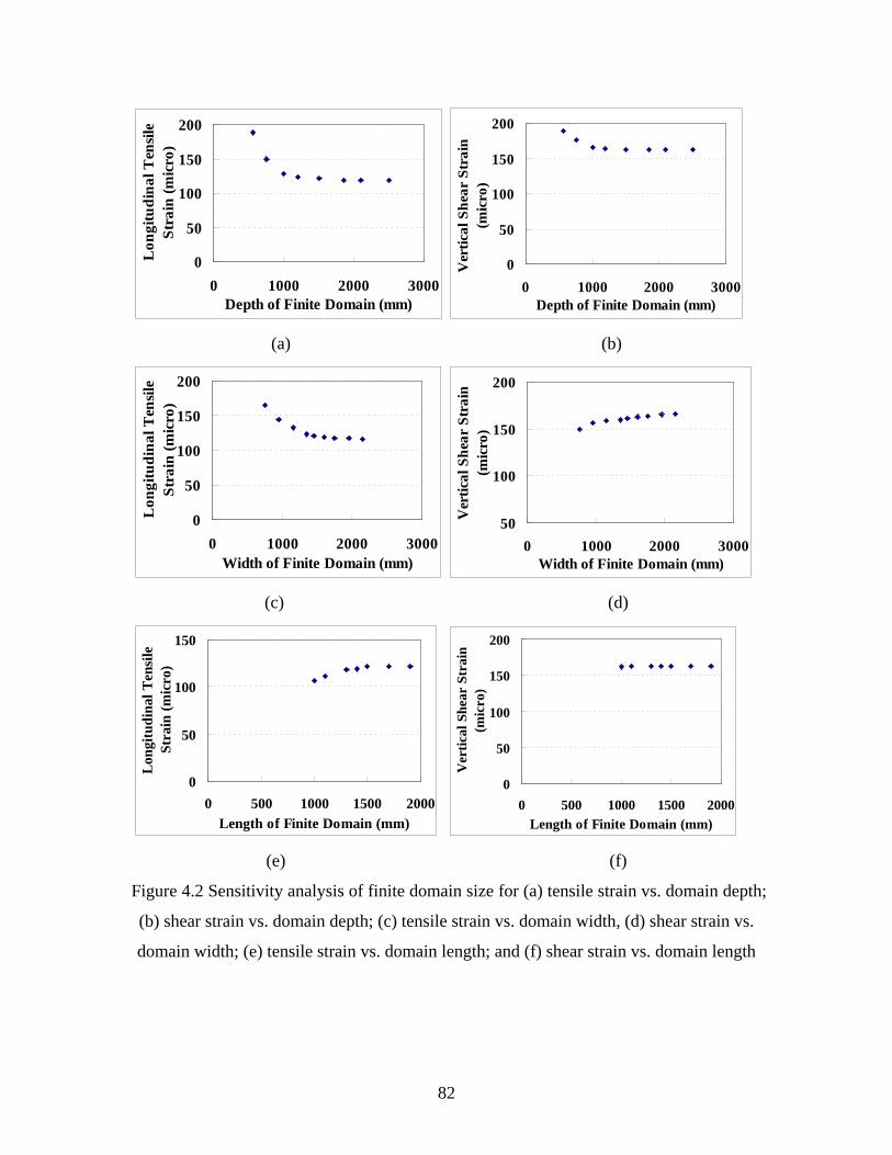
82
0
50
100
150
200
0 1000 2000 3000Depth of Finite Domain (mm)
Lon
gitu
dina
l Ten
sile
Stra
in (m
icro
)
0
50
100
150
200
0 1000 2000 3000Depth of Finite Domain (mm)
Ver
tical
She
ar S
trai
n(m
icro
)
(a) (b)
0
50
100
150
200
0 1000 2000 3000Width of Finite Domain (mm)
Lon
gitu
dina
l Ten
sile
Stra
in (m
icro
)
50
100
150
200
0 1000 2000 3000Width of Finite Domain (mm)
Ver
tical
She
ar S
trai
n(m
icro
)
(c) (d)
0
50
100
150
0 500 1000 1500 2000Length of Finite Domain (mm)
Lon
gitu
dina
l Ten
sile
Stra
in (m
icro
)
0
50
100
150
200
0 500 1000 1500 2000Length of Finite Domain (mm)
Ver
tical
She
ar S
trai
n(m
icro
)
(e) (f)
Figure 4.2 Sensitivity analysis of finite domain size for (a) tensile strain vs. domain depth;
(b) shear strain vs. domain depth; (c) tensile strain vs. domain width, (d) shear strain vs.
domain width; (e) tensile strain vs. domain length; and (f) shear strain vs. domain length
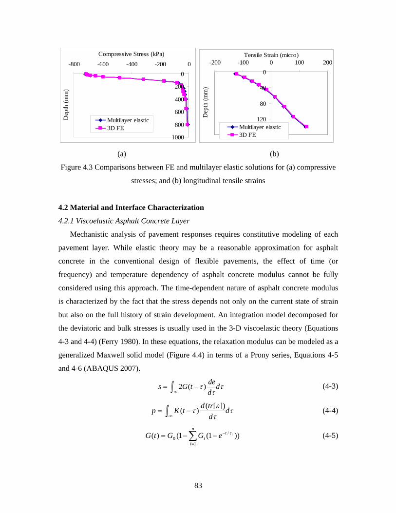
83
0
200
400
600
800
1000
-800 -600 -400 -200 0Compressive Stress (kPa)
Dep
th (m
m)
Multilayer elastic3D FE
0
40
80
120
160
-200 -100 0 100 200Tensile Strain (micro)
Dep
th (m
m)
Multilayer elastic3D FE
(a) (b)
Figure 4.3 Comparisons between FE and multilayer elastic solutions for (a) compressive
stresses; and (b) longitudinal tensile strains
4.2 Material and Interface Characterization
4.2.1 Viscoelastic Asphalt Concrete Layer
Mechanistic analysis of pavement responses requires constitutive modeling of each
pavement layer. While elastic theory may be a reasonable approximation for asphalt
concrete in the conventional design of flexible pavements, the effect of time (or
frequency) and temperature dependency of asphalt concrete modulus cannot be fully
considered using this approach. The time-dependent nature of asphalt concrete modulus
is characterized by the fact that the stress depends not only on the current state of strain
but also on the full history of strain development. An integration model decomposed for
the deviatoric and bulk stresses is usually used in the 3-D viscoelastic theory (Equations
4-3 and 4-4) (Ferry 1980). In these equations, the relaxation modulus can be modeled as a
generalized Maxwell solid model (Figure 4.4) in terms of a Prony series, Equations 4-5
and 4-6 (ABAQUS 2007).
ττ
τ dddetGs
t
∫ ∞−−= )(2 (4-3)
ττετ d
dtrdtKp
t
∫ ∞−−=
])[()( (4-4)
))1(1()( /
10
itn
ii eGGtG τ−
=
−−= ∑ (4-5)
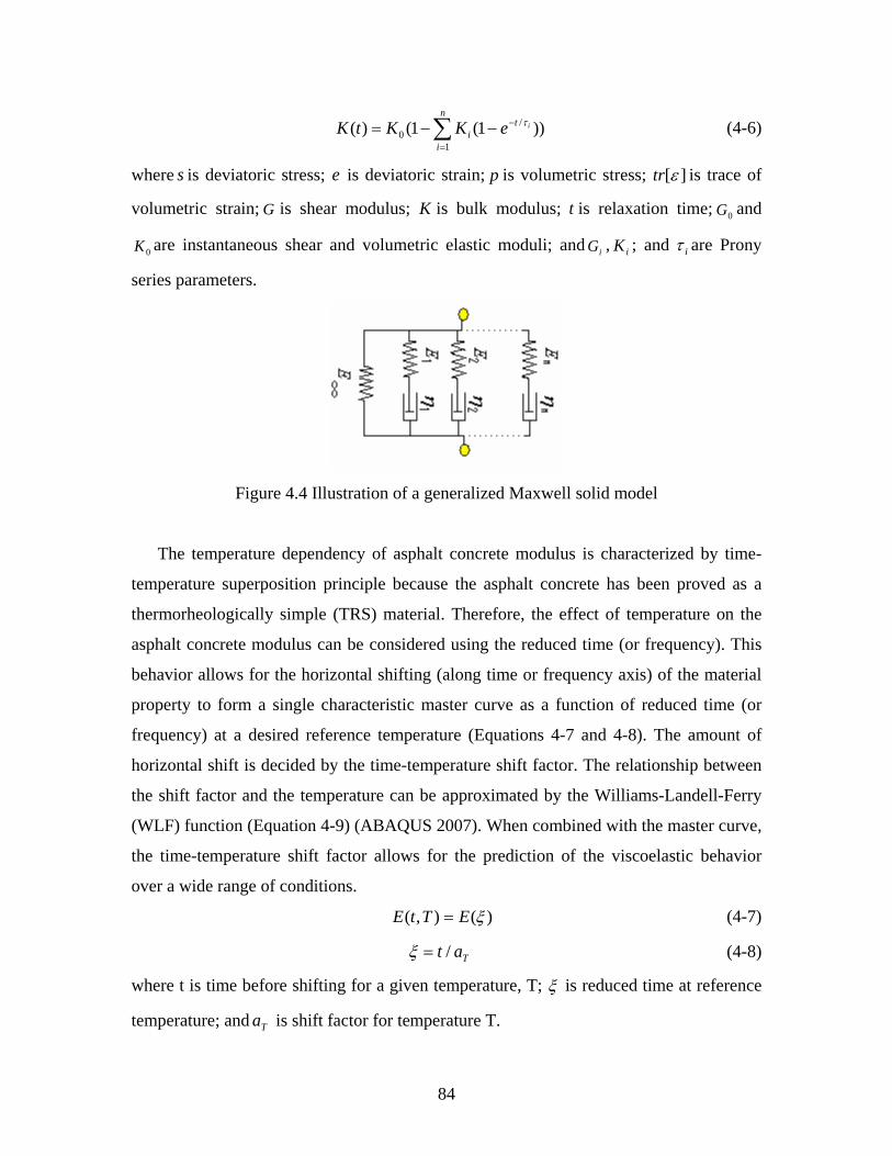
84
))1(1()( /
10
itn
ii eKKtK τ−
=
−−= ∑ (4-6)
where s is deviatoric stress; e is deviatoric strain; p is volumetric stress; ][εtr is trace of
volumetric strain; G is shear modulus; K is bulk modulus; t is relaxation time; 0G and
0K are instantaneous shear and volumetric elastic moduli; and iG , iK ; and iτ are Prony
series parameters.
Figure 4.4 Illustration of a generalized Maxwell solid model
The temperature dependency of asphalt concrete modulus is characterized by time-
temperature superposition principle because the asphalt concrete has been proved as a
thermorheologically simple (TRS) material. Therefore, the effect of temperature on the
asphalt concrete modulus can be considered using the reduced time (or frequency). This
behavior allows for the horizontal shifting (along time or frequency axis) of the material
property to form a single characteristic master curve as a function of reduced time (or
frequency) at a desired reference temperature (Equations 4-7 and 4-8). The amount of
horizontal shift is decided by the time-temperature shift factor. The relationship between
the shift factor and the temperature can be approximated by the Williams-Landell-Ferry
(WLF) function (Equation 4-9) (ABAQUS 2007). When combined with the master curve,
the time-temperature shift factor allows for the prediction of the viscoelastic behavior
over a wide range of conditions.
)(),( ξETtE = (4-7)
Tat /=ξ (4-8)
where t is time before shifting for a given temperature, T; ξ is reduced time at reference
temperature; and Ta is shift factor for temperature T.
85
)()()log(02
01
TTCTTCaT −+
−−= (4-9)
where T0 is reference temperature; T is actual temperature corresponding to the shift
factor; and C1, C2 are regression parameters.
The viscoelastic property of asphalt concrete can be predicted using the time-
dependent creep compliance test, or the frequency-dependent complex modulus test.
Different laboratory setups are available for conducting these tests: uniaxial, triaxial, or
indirect tensile (IDT). The indirect tensile setup was used in this study to allow testing
thin asphalt layer cores taken from the field. The test specimens were cut from the field
cores and have the dimensions of 152mm in diameter by 51mm in height.
The IDT creep tests were performed at five temperatures (-15, -5, 5, 15, and 25°C) for
100s under a constant load (Figure 4.5). Stress/strain levels applied to the specimens were
kept low enough to ensure minimum damage during the entire testing period, and
therefore, linear viscoelastic behavior. The creep compliance [D(t)] was calculated based
on the measured deformations using the AASHTO T322 method (Buttlar and Roque
1994). Master creep curves were constructed by horizontally shifting the creep curves at
various temperatures to the creep curve at the reference temperature of 25°C.
The relaxation modulus E(t) is the ratio of stress response to a constant strain input,
while the creep compliance, D(t), is the ratio of the strain response to a constant stress
input. For a purely elastic material, E(t) and D(t) are reciprocals. However, for the
viscoelastic material, this is only true in the Laplace transform domain. Ferry (1980)
showed that there is an exact relationship between the creep compliance and relaxation
modulus using the convolution integral in Equation 4-10.
0( ) ( )
tE t D d tτ τ τ− =∫ for t>0 (4-10)
An approximate method can be used to convert from creep compliance to relaxation
modulus if both the creep compliance and relaxation modulus are modeled using a power
law analytical form, as shown in Equation 4-11. Practically, the laboratory-determined
creep compliance is not exactly represented by power law function. In this case, the local
slope of the power model can be determined using Equation 4-12 (Park and Kim 1999).
The bulk (K) and shear (G) relaxation modulus are calculated from relaxation modulus (E)
assuming a constant Poisson’s ratio and fitted into the Prony series as a generalized
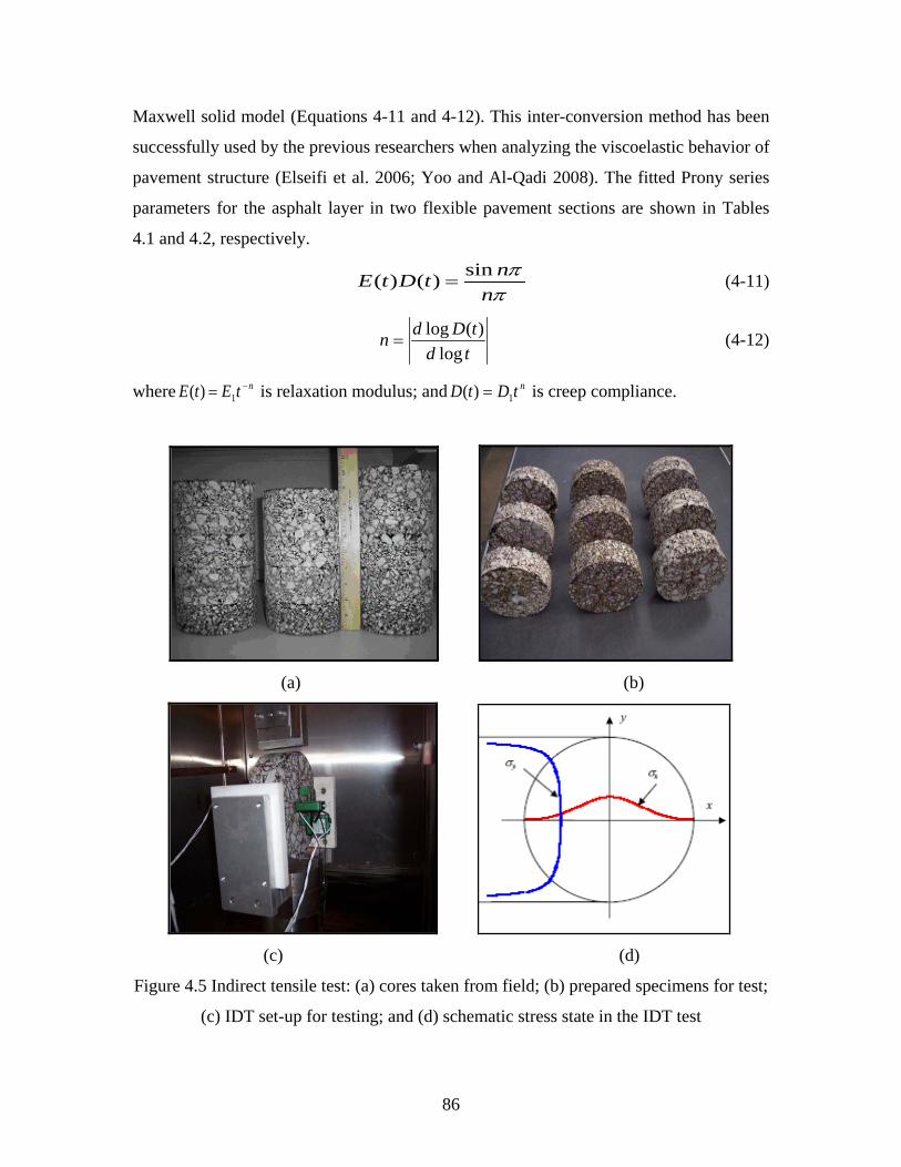
86
Maxwell solid model (Equations 4-11 and 4-12). This inter-conversion method has been
successfully used by the previous researchers when analyzing the viscoelastic behavior of
pavement structure (Elseifi et al. 2006; Yoo and Al-Qadi 2008). The fitted Prony series
parameters for the asphalt layer in two flexible pavement sections are shown in Tables
4.1 and 4.2, respectively.
sin( ) ( ) nE t D tnπ
π= (4-11)
tdtDdn
log)(log
= (4-12)
where ntEtE −= 1)( is relaxation modulus; and ntDtD 1)( = is creep compliance.
(a) (b)
(c) (d)
Figure 4.5 Indirect tensile test: (a) cores taken from field; (b) prepared specimens for test;
(c) IDT set-up for testing; and (d) schematic stress state in the IDT test
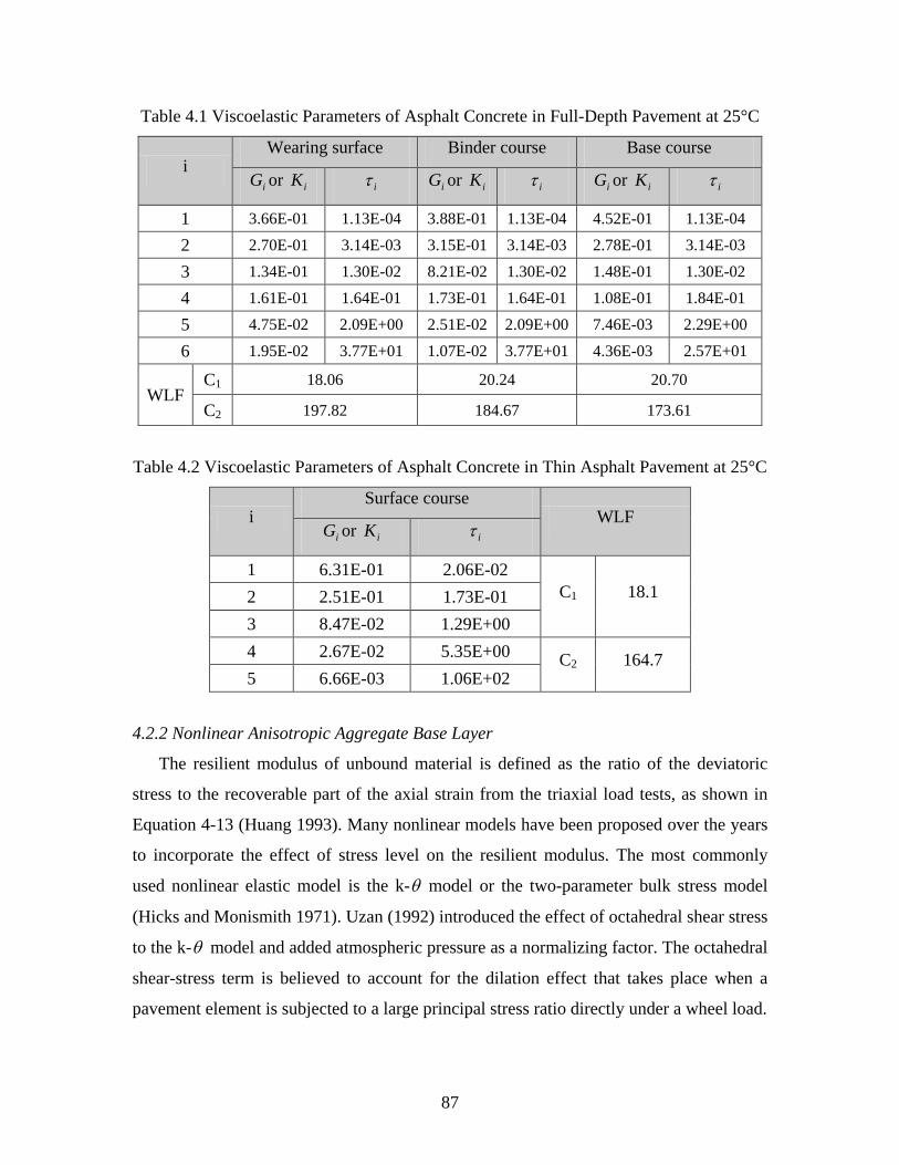
87
Table 4.1 Viscoelastic Parameters of Asphalt Concrete in Full-Depth Pavement at 25°C
i Wearing surface Binder course Base course
iG or iK iτ iG or iK iτ iG or iK iτ
1 3.66E-01 1.13E-04 3.88E-01 1.13E-04 4.52E-01 1.13E-04
2 2.70E-01 3.14E-03 3.15E-01 3.14E-03 2.78E-01 3.14E-03
3 1.34E-01 1.30E-02 8.21E-02 1.30E-02 1.48E-01 1.30E-02
4 1.61E-01 1.64E-01 1.73E-01 1.64E-01 1.08E-01 1.84E-01
5 4.75E-02 2.09E+00 2.51E-02 2.09E+00 7.46E-03 2.29E+00
6 1.95E-02 3.77E+01 1.07E-02 3.77E+01 4.36E-03 2.57E+01
WLF C1 18.06 20.24 20.70
C2 197.82 184.67 173.61
Table 4.2 Viscoelastic Parameters of Asphalt Concrete in Thin Asphalt Pavement at 25°C
i Surface course
WLF iG or iK iτ
1 6.31E-01 2.06E-02 C1 18.1 2 2.51E-01 1.73E-01
3 8.47E-02 1.29E+00 4 2.67E-02 5.35E+00 C2 164.7 5 6.66E-03 1.06E+02
4.2.2 Nonlinear Anisotropic Aggregate Base Layer
The resilient modulus of unbound material is defined as the ratio of the deviatoric
stress to the recoverable part of the axial strain from the triaxial load tests, as shown in
Equation 4-13 (Huang 1993). Many nonlinear models have been proposed over the years
to incorporate the effect of stress level on the resilient modulus. The most commonly
used nonlinear elastic model is the k-θ model or the two-parameter bulk stress model
(Hicks and Monismith 1971). Uzan (1992) introduced the effect of octahedral shear stress
to the k-θ model and added atmospheric pressure as a normalizing factor. The octahedral
shear-stress term is believed to account for the dilation effect that takes place when a
pavement element is subjected to a large principal stress ratio directly under a wheel load.
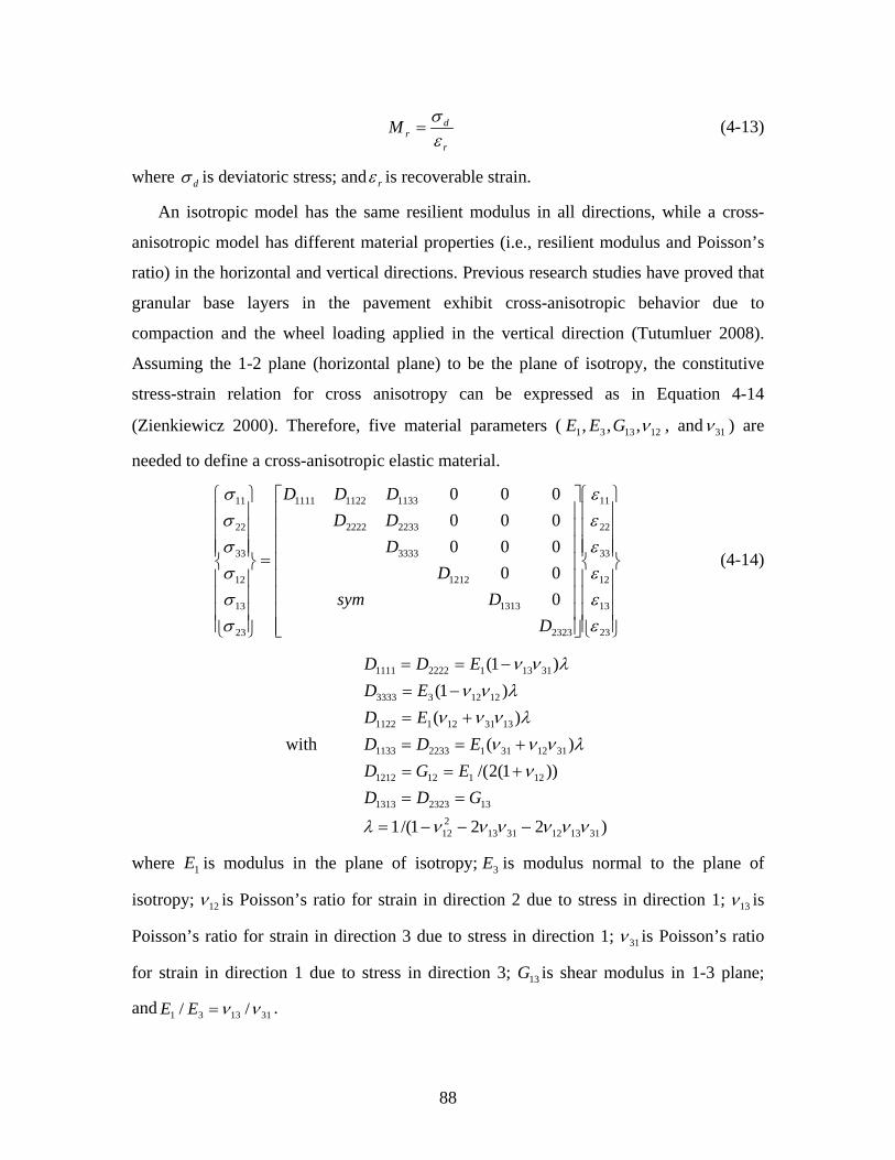
88
r
drM
εσ
= (4-13)
where dσ is deviatoric stress; and rε is recoverable strain.
An isotropic model has the same resilient modulus in all directions, while a cross-
anisotropic model has different material properties (i.e., resilient modulus and Poisson’s
ratio) in the horizontal and vertical directions. Previous research studies have proved that
granular base layers in the pavement exhibit cross-anisotropic behavior due to
compaction and the wheel loading applied in the vertical direction (Tutumluer 2008).
Assuming the 1-2 plane (horizontal plane) to be the plane of isotropy, the constitutive
stress-strain relation for cross anisotropy can be expressed as in Equation 4-14
(Zienkiewicz 2000). Therefore, five material parameters ( 121331 ,,, νGEE , and 31ν ) are
needed to define a cross-anisotropic elastic material.
=
23
13
12
33
22
11
2323
1313
1212
3333
22332222
113311221111
23
13
12
33
22
11
000000000000
εεεεεε
σσσσσσ
DDsym
DDDDDDD
(4-14)
with
)221/(1
))1(2/()(
)()1(
)1(
3113123113212
1323231313
121121212
311231122331133
13311211122
121233333
3113122221111
ννννννλ
νλννν
λνννλνν
λνν
−−−=
==+==+==
+=−=
−==
GDDEGD
EDDEDED
EDD
where 1E is modulus in the plane of isotropy; 3E is modulus normal to the plane of
isotropy; 12ν is Poisson’s ratio for strain in direction 2 due to stress in direction 1; 13ν is
Poisson’s ratio for strain in direction 3 due to stress in direction 1; 31ν is Poisson’s ratio
for strain in direction 1 due to stress in direction 3; 13G is shear modulus in 1-3 plane;
and 311331 // νν=EE .
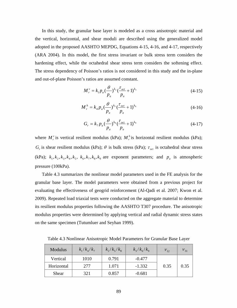
89
In this study, the granular base layer is modeled as a cross anisotropic material and
the vertical, horizontal, and shear moduli are described using the generalized model
adopted in the proposed AASHTO MEPDG, Equations 4-15, 4-16, and 4-17, respectively
(ARA 2004). In this model, the first stress invariant or bulk stress term considers the
hardening effect, while the octahedral shear stress term considers the softening effect.
The stress dependency of Poisson’s ratios is not considered in this study and the in-plane
and out-of-plane Poisson’s ratios are assumed constant.
32 )1()(1k
a
octk
aa
vr pp
pkM +=τθ
(4-15)
65 )1()(4k
a
octk
aa
hr pp
pkM +=τθ
(4-16)
98 )1()(7k
a
octk
aar pp
pkG +=τθ
(4-17)
where vrM is vertical resilient modulus (kPa); h
rM is horizontal resilient modulus (kPa);
rG is shear resilient modulus (kPa); θ is bulk stress (kPa); octτ is octahedral shear stress
(kPa); ,,,,, 54321 kkkkk 9876 ,,, kkkk are exponent parameters; and ap is atmospheric
pressure (100kPa).
Table 4.3 summarizes the nonlinear model parameters used in the FE analysis for the
granular base layer. The model parameters were obtained from a previous project for
evaluating the effectiveness of geogrid reinforcement (Al-Qadi et al. 2007; Kwon et al.
2009). Repeated load triaxial tests were conducted on the aggregate material to determine
its resilient modulus properties following the AASHTO T307 procedure. The anisotropic
modulus properties were determined by applying vertical and radial dynamic stress states
on the same specimen (Tutumluer and Seyhan 1999).
Table 4.3 Nonlinear Anisotropic Model Parameters for Granular Base Layer
Modulus 1k / 4k / 7k 2k / 5k / 8k 3k / 6k / 9k 12ν 31ν
Vertical 1010 0.791 -0.477 0.35 0.35 Horizontal 277 1.071 -1.332
Shear 321 0.857 -0.681
90
4.2.3 Subgrade Modulus
Typically, the modulus of fine-grained soil decrease as stress levels increase and thus
show the stress-softening behavior. The softening behavior of the subgrade is important
when the stress level in the subgrade is relatively high, such as in thin asphalt pavements.
A nonlinear stress-dependent model is used for subgrade stiffness (Equation 4-18), that is
similar to the one used for the granular base layer with 2k =0. The coefficients ( 1k =0.8125
and 3k =-11.5) were estimated from the bilinear model parameters (Thompson and
Robnett 1979), which was used by Kwon et al. (2009) in the previous research.
3)1(1k
a
octaR p
pkM +=τ
(4-18)
In order to compare the model results using both linear and nonlinear subgrade
models, the linear elastic modulus of the subgrade in the thin asphalt pavement section
was estimated from its California Bearing Ratio (CBR) value using the equation in the
AASHTO MEPDG, Equation 4-19 (ARA 2004). 64.0)(2555 CBRM R = (4-19)
where MR is resilient modulus of subgrade in psi; and CBR is California Bearing Ratio of
subgrade in percentage.
The subgrade in the full-depth pavement section is modeled having linear elastic
modulus considering the stress transmitted into the subgrade under a thick asphalt layer is
relatively small. The falling weight deflectometer (FWD) test results were used to back-
calculate the linear elastic modulus of the subgrade. The back-calculated subgrade
modulus is 393MPa for the lime-stabilized layer and 173MPa for the deeper natural soil.
4.2.4 Interface Model
Contact conditions at layer interfaces are important parameters that could
significantly affect pavement responses to vehicular loading. It is expected that the layers
within the pavement structure remains in contact with no gap-opening since the contact
area is very large and high compressive loading is applied by vehicles. This assumption
was controlled by the “no separation” feature supported by ABAQUS. In addition, it is
assumed that both relative and absolute motions of contacting surfaces at layer interfaces
are small.
91
The interface bonding between asphalt layers is significantly affected by the type and
quantity of tack coat and construction quality. In this study, the HMA layers were
assumed to be fully-bonded (tied) in the thick asphalt pavement, which is validated by
field core inspection from test sections. The Coulomb friction model with a friction
coefficient of 1.0 was used at the HMA-base interface (Romanoschi and Metcalf 2001).
The coefficient of friction (µ) is defined as the ratio of the allowed maximum shear stress
before the interface slides and the normal stress, as shown in Equation 4-20.
µ = στ /max (4-20)
where maxτ is allowed maximum shear stress before sliding; and σ is normal stress at the
interface.
4.3 Nonlinear Solution Technique
Several solution techniques have been used to solve the nonlinearity problem of the
granular material. Tutumluer (1995) recommended that a direct secant stiffness method
(also known as a fixed point iteration method) with a damped factor should be used due
to the hardening nature of the granular material. The direct secant stiffness method solves
the nonlinear load displacement behavior by updating the secant stiffness at each iteration
until that a convergence is reached for the load increment. Kim and Tutumluer (2008)
further developed a user material subroutine (UMAT) in ABAQUS by utilizing the direct
secant stiffness approach. Hjelmstad and Taciroglu (2000) analyzed the nonlinear flexible
pavement responses using a Newton-Raphson approach with tangent stiffness. In their
approach, the nonlinear stress-dependent model of the granular base layer was formulated
as a function of strain states not stresses. Schwartz (2002) employed the hypoelastic
material model in ABAQUS to simulate the nonlinear behavior of the granular material.
The nonlinear stress-dependent modulus of the granular material was numerically
converted to tangent modulus for input as a function of the first stress invariant.
ABAQUS/Standard uses the iterative Newton-Raphson method to solve nonlinear
equations. The applied load is augmented incrementally, and at each increment the
program solves a system of equations through iterations. The iterations continue on the
basis of the previous solutions until it reaches a reasonable convergence (ABAQUS
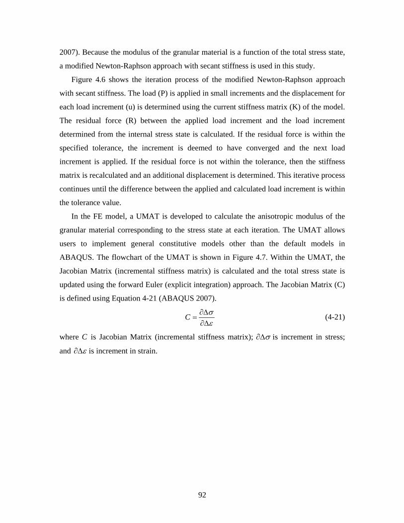
92
2007). Because the modulus of the granular material is a function of the total stress state,
a modified Newton-Raphson approach with secant stiffness is used in this study.
Figure 4.6 shows the iteration process of the modified Newton-Raphson approach
with secant stiffness. The load (P) is applied in small increments and the displacement for
each load increment (u) is determined using the current stiffness matrix (K) of the model.
The residual force (R) between the applied load increment and the load increment
determined from the internal stress state is calculated. If the residual force is within the
specified tolerance, the increment is deemed to have converged and the next load
increment is applied. If the residual force is not within the tolerance, then the stiffness
matrix is recalculated and an additional displacement is determined. This iterative process
continues until the difference between the applied and calculated load increment is within
the tolerance value.
In the FE model, a UMAT is developed to calculate the anisotropic modulus of the
granular material corresponding to the stress state at each iteration. The UMAT allows
users to implement general constitutive models other than the default models in
ABAQUS. The flowchart of the UMAT is shown in Figure 4.7. Within the UMAT, the
Jacobian Matrix (incremental stiffness matrix) is calculated and the total stress state is
updated using the forward Euler (explicit integration) approach. The Jacobian Matrix (C)
is defined using Equation 4-21 (ABAQUS 2007).
εσ∆∂∆∂
=C (4-21)
where C is Jacobian Matrix (incremental stiffness matrix); σ∆∂ is increment in stress;
and ε∆∂ is increment in strain.
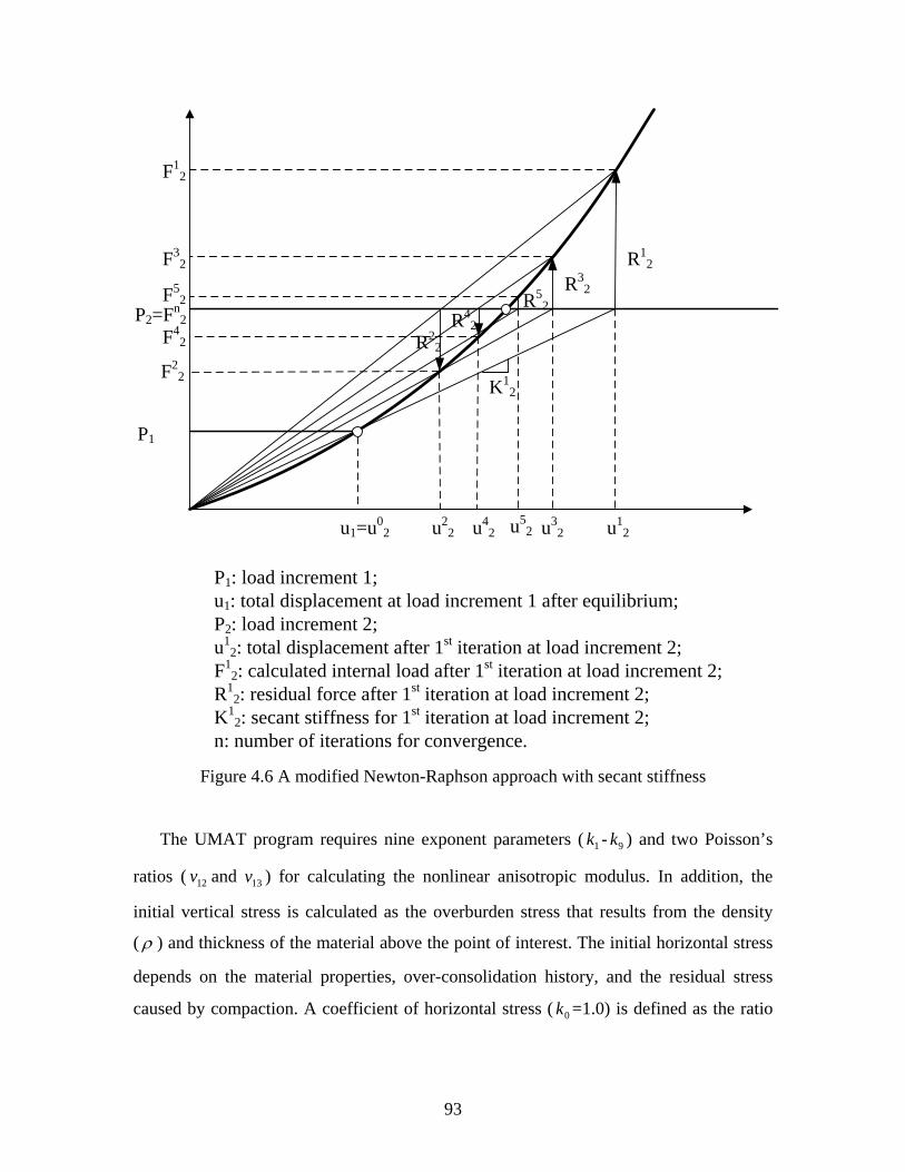
93
P1: load increment 1;u1: total displacement at load increment 1 after equilibrium;P2: load increment 2;u1
2: total displacement after 1st iteration at load increment 2;F1
2: calculated internal load after 1st iteration at load increment 2;R1
2: residual force after 1st iteration at load increment 2;K1
2: secant stiffness for 1st iteration at load increment 2;n: number of iterations for convergence.
P1
P2=Fn2
F12
R12
u1=u02 u1
2u22 u3
2
R32
R22
R42
u42
R52
u52
F42
F32
F22
F52
K12
Figure 4.6 A modified Newton-Raphson approach with secant stiffness
The UMAT program requires nine exponent parameters ( 1k - 9k ) and two Poisson’s
ratios ( 12v and 13v ) for calculating the nonlinear anisotropic modulus. In addition, the
initial vertical stress is calculated as the overburden stress that results from the density
( ρ ) and thickness of the material above the point of interest. The initial horizontal stress
depends on the material properties, over-consolidation history, and the residual stress
caused by compaction. A coefficient of horizontal stress ( 0k =1.0) is defined as the ratio
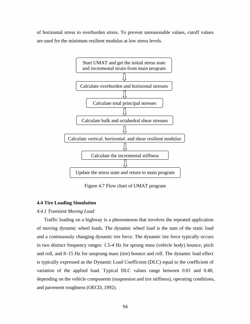
94
of horizontal stress to overburden stress. To prevent unreasonable values, cutoff values
are used for the minimum resilient modulus at low stress levels.
Figure 4.7 Flow chart of UMAT program
4.4 Tire Loading Simulation
4.4.1 Transient Moving Load
Traffic loading on a highway is a phenomenon that involves the repeated application
of moving dynamic wheel loads. The dynamic wheel load is the sum of the static load
and a continuously changing dynamic tire force. The dynamic tire force typically occurs
in two distinct frequency ranges: 1.5-4 Hz for sprung mass (vehicle body) bounce, pitch
and roll, and 8–15 Hz for unsprung mass (tire) bounce and roll. The dynamic load effect
is typically expressed as the Dynamic Load Coefficient (DLC) equal to the coefficient of
variation of the applied load. Typical DLC values range between 0.01 and 0.40,
depending on the vehicle components (suspension and tire stiffness), operating conditions,
and pavement roughness (OECD, 1992).
Calculate total principal stresses
Calculate bulk and octahedral shear stresses
Calculate vertical, horizontal, and shear resilient modulus
Calculate the incremental stiffness
Update the stress state and return to main program
Start UMAT and get the initial stress state and incremental strain from main program
Calculate overburden and horizontal stresses
95
To define the dynamic wheel load, intensive field measurements from vehicle axles
are needed. For pavement specialists, most studies are focused on measuring dynamic
tire-pavement contact stresses rather than the stochastic distribution of dynamic wheel
loads. In order to characterize the transient local dynamic load without extensive field
data in this study, the dynamic loading is simplified by using the measured and predicted
tire contact stresses on a smooth pavement surface.
There are several methods that can be used to simulate vehicular loading: stationary
constant load; moving constant load; stationary transient load (triangle, trapezoidal, or
haversine function); and moving transient load. The load applied by the vehicle is in
nature a continuously changing moving load as the vehicle is approaching and leaving.
To simulate the nature of moving vehicular loading at a certain speed, the concept of
continuously moving load (Yoo and Al-Qadi 2008) is used in this study.
In this approach, the loading area is gradually shifted over the pavement surface at
each step until a single wheel pass is completed, as shown in Figure 4.8. At each loading
step, a linear loading amplitude was applied to accurately simulate the variation of
contact stresses in the tire imprint area. Different loading amplitude paths were used to
define the entrance and the exit parts of the tire imprint, respectively.
For example, the tire imprint of rib A is composed of nine elements (A1-A8) and A9
is the element that the tire is approaching. As the vehicle approaches a given element in
the loading path, the element is loaded with the amplitude that simulates the increase in
loading with time (A6-A9). Similarly, as the tire moves away from a given element, the
loading amplitude that simulates the decrease in loading with time is used (A1-A4). For
each loading step, the tire imprint area is maintained constant. The step time is decided
by the vehicle speed and element lengths. The time increment in each step is selected to
satisfy the time integration requirement for implicit dynamic analysis and the
convergence requirement for the nonlinear iteration.
4.4.2 Incorporation of Tire-Pavement Contact Stresses
In the FE model, the 3-D tire-pavement contact stresses (vertical, transverse, and
longitudinal) under each rib were applied on the tire imprint area, respectively (Figure
4.9). The exact footprint shape at a specific load and tire pressure level is considered by
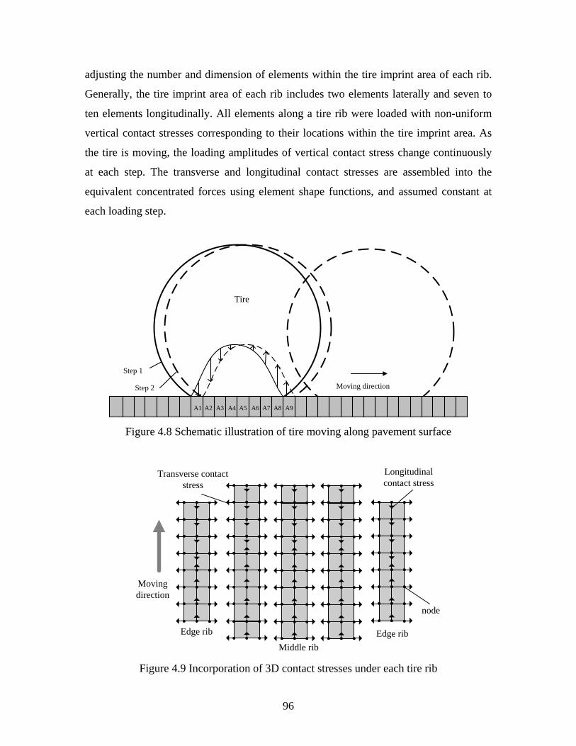
96
adjusting the number and dimension of elements within the tire imprint area of each rib.
Generally, the tire imprint area of each rib includes two elements laterally and seven to
ten elements longitudinally. All elements along a tire rib were loaded with non-uniform
vertical contact stresses corresponding to their locations within the tire imprint area. As
the tire is moving, the loading amplitudes of vertical contact stress change continuously
at each step. The transverse and longitudinal contact stresses are assembled into the
equivalent concentrated forces using element shape functions, and assumed constant at
each loading step.
Step 1
Step 2
Tire
A1 A8A7A6A5A4A3A2 A9
Moving direction
Figure 4.8 Schematic illustration of tire moving along pavement surface
node
Middle rib
Edge rib Edge rib
Longitudinal contact stress
Transverse contact stress
Moving direction
Figure 4.9 Incorporation of 3D contact stresses under each tire rib
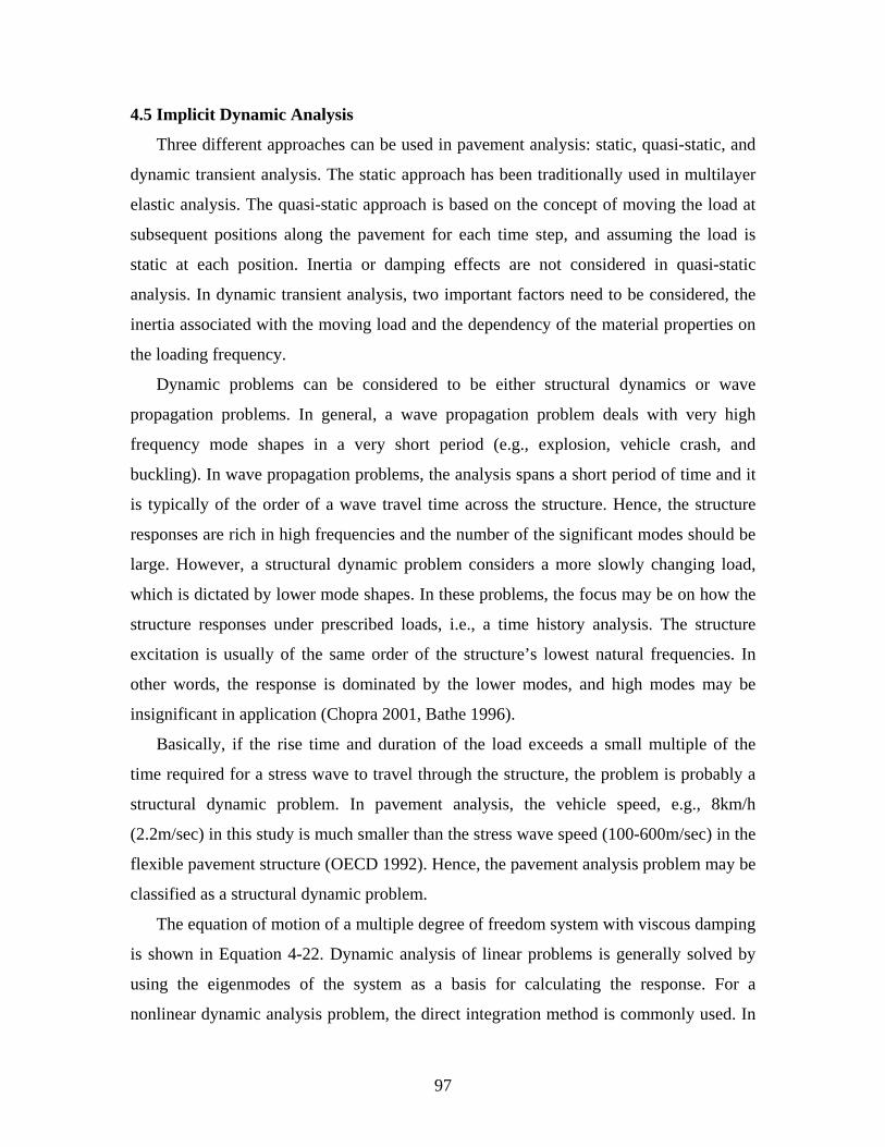
97
4.5 Implicit Dynamic Analysis
Three different approaches can be used in pavement analysis: static, quasi-static, and
dynamic transient analysis. The static approach has been traditionally used in multilayer
elastic analysis. The quasi-static approach is based on the concept of moving the load at
subsequent positions along the pavement for each time step, and assuming the load is
static at each position. Inertia or damping effects are not considered in quasi-static
analysis. In dynamic transient analysis, two important factors need to be considered, the
inertia associated with the moving load and the dependency of the material properties on
the loading frequency.
Dynamic problems can be considered to be either structural dynamics or wave
propagation problems. In general, a wave propagation problem deals with very high
frequency mode shapes in a very short period (e.g., explosion, vehicle crash, and
buckling). In wave propagation problems, the analysis spans a short period of time and it
is typically of the order of a wave travel time across the structure. Hence, the structure
responses are rich in high frequencies and the number of the significant modes should be
large. However, a structural dynamic problem considers a more slowly changing load,
which is dictated by lower mode shapes. In these problems, the focus may be on how the
structure responses under prescribed loads, i.e., a time history analysis. The structure
excitation is usually of the same order of the structure’s lowest natural frequencies. In
other words, the response is dominated by the lower modes, and high modes may be
insignificant in application (Chopra 2001, Bathe 1996).
Basically, if the rise time and duration of the load exceeds a small multiple of the
time required for a stress wave to travel through the structure, the problem is probably a
structural dynamic problem. In pavement analysis, the vehicle speed, e.g., 8km/h
(2.2m/sec) in this study is much smaller than the stress wave speed (100-600m/sec) in the
flexible pavement structure (OECD 1992). Hence, the pavement analysis problem may be
classified as a structural dynamic problem.
The equation of motion of a multiple degree of freedom system with viscous damping
is shown in Equation 4-22. Dynamic analysis of linear problems is generally solved by
using the eigenmodes of the system as a basis for calculating the response. For a
nonlinear dynamic analysis problem, the direct integration method is commonly used. In
98
this method, the equation of motion is integrated using a numerical step-by-step
procedure at discrete time intervals. Two types of direct integration are available, explicit
and implicit. The implicit integration method computes the displacements at time t and t-
1 by solving a set of nonlinear equations simultaneously, while the explicit integration
computes the displacement at time t by adding the incremental displacement between
time t and t-1 computed by double integration of the acceleration. The implicit dynamic
analysis is used in this study, because it provides better numerical stability than explicit
analysis and is generally efficient for structural dynamic problems (Bathe 1996).
{ } { } { } { }PUKUCUM =++ }[][][ (4-22)
where ][M is mass matrix; ][C is damping matrix; ][K is stiffness matrix; { }P is external
force vector; { }U is acceleration vector; { }U is velocity vector; and{ }U is displacement
vector.
The implicit integration method in ABAQUS uses the Newmark integration scheme
and the Hilber–Hughes–Taylor method (α -method) (ABAQUS 2007). The α -method is
unconditionally stable if the analysis parameters are chosen properly. Therefore, the
selection of time increment ( t∆ ) is only dependent on the accuracy criterion. Because
only low modes and a few intermediate modes are excited by the vehicular loading in the
pavement structure, the dynamic response contribution in the high frequencies are
negligible in the analysis. The procedure for choosing the time increment in implicit
dynamic analysis is as follows (Bathe 1996): 1) identifying the dominant frequency ( f )
in the loading or responses of a structure; 2) selecting the time increment ( t∆ ) less than
or equal to f20
1 . For example, as the vehicle speed is 8kmh, the time increment should
be less than 0.005sec because the highest loading frequency is usually less than 10Hz.
The dynamic analysis considers the mass inertia effect and damping effect. As shown
in Equation 4-22, the inertial force is equal to the mass multiplied by the acceleration,
whereby the acceleration is the second derivative of the displacement. The dissipative
contribution depends on the damping properties. The sources of damping can be an
arbitrary damping factor, a friction factor, or a viscoelastic material behavior. When
using viscoelastic material behavior for an asphalt layer, it is not necessary to introduce
99
additional structural or mass damping for that layer. However, the elastic aggregate base
layer and subgrade do not have such energy dissipation sources. Therefore, introducing a
general damping rule to those layers is needed.
A popular spectral damping scheme used in structure dynamic analysis is Rayleigh
damping; giving the damping matrix [ ]C as the combination of mass-proportional
damping and stiffness-proportional damping, as shown in Equation 4-23. For multiple
degrees of freedom system, the critical damping ratio at any frequency of mode is given
as Equation 4-24. The coefficients Rα and Rβ can be determined from specific iξ and jξ
for the i th and j th modes, respectively. If both modes are assumed to have the same
damping ratioξ , the Raleigh coefficients can be calculated using Equation 4-25 (Chopra
2001).
[ ] [ ] [ ]KMC RR βα += (4-23)
22iR
i
Ri
ωβωα
ξ += (4-24)
ji
jiR ww
ww+
=2
ξα , ji
R ww +=
2ξβ (4-25)
where RR βα , are Raleigh coefficients; and iξ is critical damping ratio at the frequency
of iω .
For the dynamic loading on a pavement structure, the two frequencies in calculating
the Raleigh coefficients may be taken as the lowest natural frequency of the structure and
the highest loading frequency. The critical damping ratio of soil falls in the range of 2%
to 5% depending on the confining pressure and shear strain level, which can be measured
from the resonant column test or cyclic triaxial test (Zhong et al. 2002). Because the
granular base layer and subgrade are considered as elastic material without any other
energy dissipation sources (such as plastic), the maximum damping ratio, 5%, is used.
4.6 Comparison between Model Results and Field Measurements
Two typical pavement structures were selected in this dissertation: a thin asphalt
pavement with a granular base layer (simulating a secondary road), and a thick asphalt
pavement, such as that used for interstate highway systems. The two pavement structures
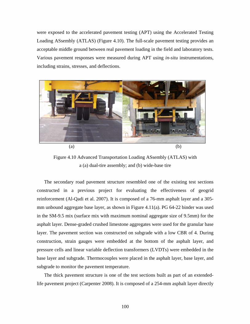
100
were exposed to the accelerated pavement testing (APT) using the Accelerated Testing
Loading ASsembly (ATLAS) (Figure 4.10). The full-scale pavement testing provides an
acceptable middle ground between real pavement loading in the field and laboratory tests.
Various pavement responses were measured during APT using in-situ instrumentations,
including strains, stresses, and deflections.
(a) (b)
Figure 4.10 Advanced Transportation Loading ASsembly (ATLAS) with
a (a) dual-tire assembly; and (b) wide-base tire
The secondary road pavement structure resembled one of the existing test sections
constructed in a previous project for evaluating the effectiveness of geogrid
reinforcement (Al-Qadi et al. 2007). It is composed of a 76-mm asphalt layer and a 305-
mm unbound aggregate base layer, as shown in Figure 4.11(a). PG 64-22 binder was used
in the SM-9.5 mix (surface mix with maximum nominal aggregate size of 9.5mm) for the
asphalt layer. Dense-graded crushed limestone aggregates were used for the granular base
layer. The pavement section was constructed on subgrade with a low CBR of 4. During
construction, strain gauges were embedded at the bottom of the asphalt layer, and
pressure cells and linear variable deflection transformers (LVDTs) were embedded in the
base layer and subgrade. Thermocouples were placed in the asphalt layer, base layer, and
subgrade to monitor the pavement temperature.
The thick pavement structure is one of the test sections built as part of an extended-
life pavement project (Carpenter 2008). It is composed of a 254-mm asphalt layer directly
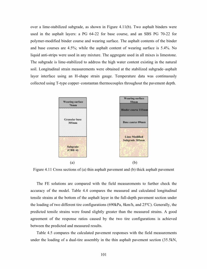
101
over a lime-stabilized subgrade, as shown in Figure 4.11(b). Two asphalt binders were
used in the asphalt layers: a PG 64-22 for base course, and an SBS PG 70-22 for
polymer-modified binder course and wearing surface. The asphalt contents of the binder
and base courses are 4.5%; while the asphalt content of wearing surface is 5.4%. No
liquid anti-strips were used in any mixture. The aggregate used in all mixes is limestone.
The subgrade is lime-stabilized to address the high water content existing in the natural
soil. Longitudinal strain measurements were obtained at the stabilized subgrade–asphalt
layer interface using an H-shape strain gauge. Temperature data was continuously
collected using T-type copper–constantan thermocouples throughout the pavement depth.
(a) (b)
Figure 4.11 Cross sections of (a) thin asphalt pavement and (b) thick asphalt pavement
The FE solutions are compared with the field measurements to further check the
accuracy of the model. Table 4.4 compares the measured and calculated longitudinal
tensile strains at the bottom of the asphalt layer in the full-depth pavement section under
the loading of two different tire configurations (690kPa, 8km/h, and 25ºC). Generally, the
predicted tensile strains were found slightly greater than the measured strains. A good
agreement of the response ratios caused by the two tire configurations is achieved
between the predicted and measured results.
Table 4.5 compares the calculated pavement responses with the field measurements
under the loading of a dual-tire assembly in the thin asphalt pavement section (35.5kN,
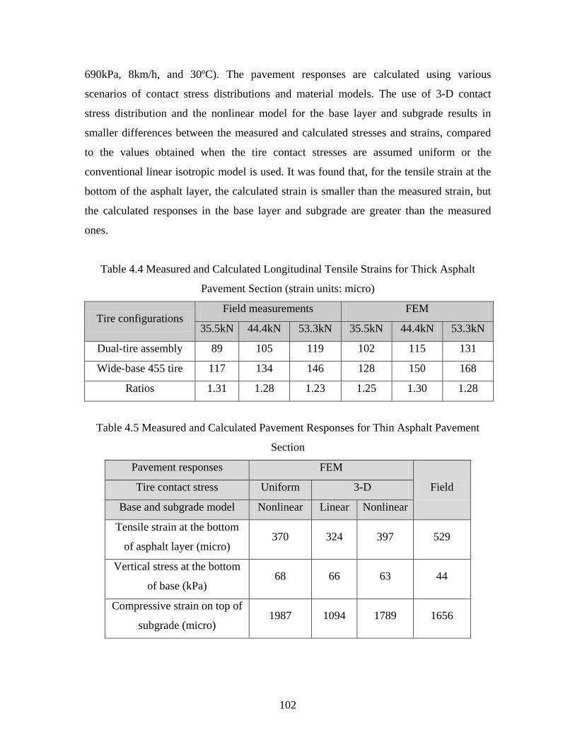
102
690kPa, 8km/h, and 30ºC). The pavement responses are calculated using various
scenarios of contact stress distributions and material models. The use of 3-D contact
stress distribution and the nonlinear model for the base layer and subgrade results in
smaller differences between the measured and calculated stresses and strains, compared
to the values obtained when the tire contact stresses are assumed uniform or the
conventional linear isotropic model is used. It was found that, for the tensile strain at the
bottom of the asphalt layer, the calculated strain is smaller than the measured strain, but
the calculated responses in the base layer and subgrade are greater than the measured
ones.
Table 4.4 Measured and Calculated Longitudinal Tensile Strains for Thick Asphalt
Pavement Section (strain units: micro)
Tire configurations Field measurements FEM
35.5kN 44.4kN 53.3kN 35.5kN 44.4kN 53.3kN
Dual-tire assembly 89 105 119 102 115 131
Wide-base 455 tire 117 134 146 128 150 168
Ratios 1.31 1.28 1.23 1.25 1.30 1.28
Table 4.5 Measured and Calculated Pavement Responses for Thin Asphalt Pavement
Section
Pavement responses FEM
Field Tire contact stress Uniform 3-D
Base and subgrade model Nonlinear Linear Nonlinear
Tensile strain at the bottom
of asphalt layer (micro) 370 324 397 529
Vertical stress at the bottom
of base (kPa) 68 66 63 44
Compressive strain on top of
subgrade (micro) 1987 1094 1789 1656
103
The accuracy of FE analysis is affected by the material models used in the analysis.
The discrepancies between the measured and the calculated pavement responses could be
related to two reasons: 1) the nonlinear viscoelasticity of asphalt concrete was not
considered in the analysis and these factors have more significant effects on the thin
asphalt pavement responses with weak supports; 2) the measured tensile strains in the
thin asphalt layer could be overstated because at the bottom of the thin asphalt layer the
bending is more significant than tension. Considering the variability of as-built pavement
thickness, environmental conditions, laboratory-measured material stiffness, and
instrumentation responses, the discrepancies between the measured and the calculated
responses were considered acceptable in this study for the purpose of comparing
pavement responses at various tire loading conditions.
4.7 Summary
A 3-D FE model of flexible pavement is developed to analyze pavement responses
under vehicular loading. This model utilizes implicit dynamic analysis and simulates the
vehicular loading as a continuous moving load with three-dimensional contact stresses at
the tire-pavement interface. In the model, the asphalt layer is modeled as a linear
viscoelastic material and its relaxation modulus is converted from the laboratory-
determined creep compliance data. The granular base layer is modeled as a nonlinear
anisotropic material and its vertical, horizontal, and shear modulus is dependent on both
the bulk stress and shear stress. A UMAT is developed to implement the constitutive
model of the granular base layer in the FE model. The FE model results were compared
with field measurements and the discrepancies were considered acceptable for the
purpose of comparing pavement responses at various tire loading conditions.
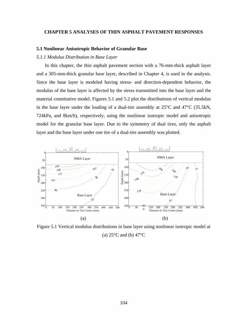
104
CHAPTER 5 ANALYSES OF THIN ASPHALT PAVEMENT RESPONSES
5.1 Nonlinear Anisotropic Behavior of Granular Base
5.1.1 Modulus Distribution in Base Layer
In this chapter, the thin asphalt pavement section with a 76-mm-thick asphalt layer
and a 305-mm-thick granular base layer, described in Chapter 4, is used in the analysis.
Since the base layer is modeled having stress- and direction-dependent behavior, the
modulus of the base layer is affected by the stress transmitted into the base layer and the
material constitutive model. Figures 5.1 and 5.2 plot the distributions of vertical modulus
in the base layer under the loading of a dual-tire assembly at 25°C and 47°C (35.5kN,
724kPa, and 8km/h), respectively, using the nonlinear isotropic model and anisotropic
model for the granular base layer. Due to the symmetry of dual tires, only the asphalt
layer and the base layer under one tire of a dual-tire assembly was plotted.
65
65
86
86
107
107
127148
169
0 50 100 150 200 250 300 350 400 450 500
0
50
100
150
200
250
300
350
Distance to Tire Center (mm)
Dep
th (m
m)
HMA Layer
Base Layer
57
87
87
118
118
148
148179
209
0 50 100 150 200 250 300 350 400 450 500
0
50
100
150
200
250
300
350
HMA Layer
Base Layer
Distance to Tire Center (mm)
Dep
th (m
m)
(a) (b)
Figure 5.1 Vertical modulus distributions in base layer using nonlinear isotropic model at
(a) 25°C and (b) 47°C
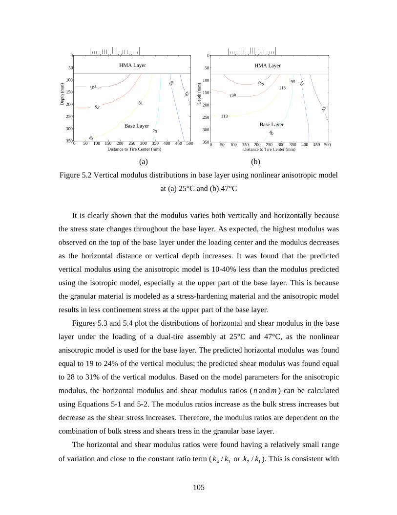
105
47
59
70
81
81
92
104
0 50 100 150 200 250 300 350 400 450 500
0
50
100
150
200
250
300
350
HMA Layer
Base Layer
Distance to Tire Center (mm)
Dep
th (m
m)
43
67
90
90113
113
136
160
0 50 100 150 200 250 300 350 400 450 500
0
50
100
150
200
250
300
350
HMA Layer
Base Layer
Distance to Tire Center (mm)
Dep
th (m
m)
(a) (b)
Figure 5.2 Vertical modulus distributions in base layer using nonlinear anisotropic model
at (a) 25°C and (b) 47°C
It is clearly shown that the modulus varies both vertically and horizontally because
the stress state changes throughout the base layer. As expected, the highest modulus was
observed on the top of the base layer under the loading center and the modulus decreases
as the horizontal distance or vertical depth increases. It was found that the predicted
vertical modulus using the anisotropic model is 10-40% less than the modulus predicted
using the isotropic model, especially at the upper part of the base layer. This is because
the granular material is modeled as a stress-hardening material and the anisotropic model
results in less confinement stress at the upper part of the base layer.
Figures 5.3 and 5.4 plot the distributions of horizontal and shear modulus in the base
layer under the loading of a dual-tire assembly at 25°C and 47°C, as the nonlinear
anisotropic model is used for the base layer. The predicted horizontal modulus was found
equal to 19 to 24% of the vertical modulus; the predicted shear modulus was found equal
to 28 to 31% of the vertical modulus. Based on the model parameters for the anisotropic
modulus, the horizontal modulus and shear modulus ratios ( n and m ) can be calculated
using Equations 5-1 and 5-2. The modulus ratios increase as the bulk stress increases but
decrease as the shear stress increases. Therefore, the modulus ratios are dependent on the
combination of bulk stress and shears tress in the granular base layer.
The horizontal and shear modulus ratios were found having a relatively small range
of variation and close to the constant ratio term ( 14 / kk or 17 / kk ). This is consistent with
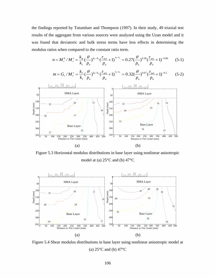
106
the findings reported by Tutumluer and Thompson (1997). In their study, 49 triaxial test
results of the aggregate from various sources were analyzed using the Uzan model and it
was found that deviatoric and bulk stress terms have less effects in determining the
modulus ratios when compared to the constant ratio term.
86.028.0
1
4 )1()(27.0)1()(/ 3625 −− +=+==
−
a
oct
aa
octkk
a
vr
hr ppppk
kMMnkk τθτθ (5-1)
2.007.0
1
7 )1()(32.0)1()(/ 3928 −− +=+==
−
a
oct
aa
octkk
a
vrr ppppk
kMGmkk τθτθ (5-2)
10
12
15
17
17
20
20
22
0 50 100 150 200 250 300 350 400 450 500
0
50
100
150
200
250
300
350
HMA Layer
Base Layer
Distance to Tire Center (mm)
Dep
th (m
m) 10
14
19
19
23
23
28
32
0 50 100 150 200 250 300 350 400 450 500
0
50
100
150
200
250
300
350
HMA Layer
Base Layer
Distance to Tire Center (mm)
Dep
th (m
m)
(a) (b)
Figure 5.3 Horizontal modulus distributions in base layer using nonlinear anisotropic
model at (a) 25°C and (b) 47°C
14
17
1721
24
24
28
28
31
0 50 100 150 200 250 300 350 400 450 500
0
50
100
150
200
250
300
350
HMA Layer
Base Layer
Distance to Tire Center (mm)
Dep
th (m
m)
12
19
19
26
26
33
33
40
40
47
0 50 100 150 200 250 300 350 400 450 500
0
50
100
150
200
250
300
350
HMA Layer
Base Layer
Distance to Tire Center (mm)
Dep
th (m
m)
(a) (b)
Figure 5.4 Shear modulus distributions in base layer using nonlinear anisotropic model at
(a) 25°C and (b) 47°C
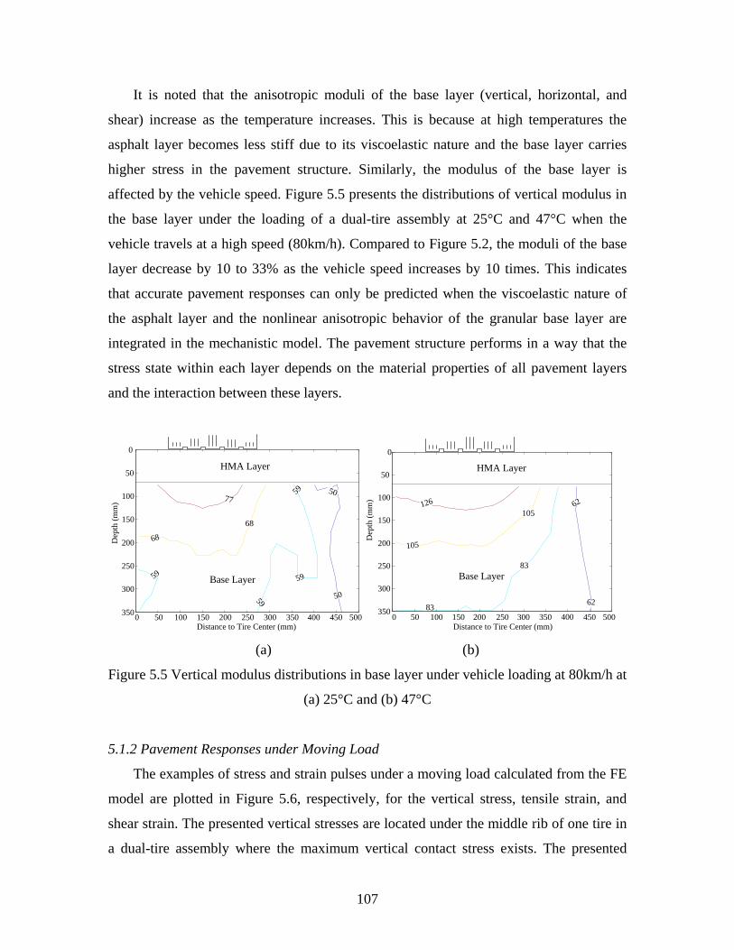
107
It is noted that the anisotropic moduli of the base layer (vertical, horizontal, and
shear) increase as the temperature increases. This is because at high temperatures the
asphalt layer becomes less stiff due to its viscoelastic nature and the base layer carries
higher stress in the pavement structure. Similarly, the modulus of the base layer is
affected by the vehicle speed. Figure 5.5 presents the distributions of vertical modulus in
the base layer under the loading of a dual-tire assembly at 25°C and 47°C when the
vehicle travels at a high speed (80km/h). Compared to Figure 5.2, the moduli of the base
layer decrease by 10 to 33% as the vehicle speed increases by 10 times. This indicates
that accurate pavement responses can only be predicted when the viscoelastic nature of
the asphalt layer and the nonlinear anisotropic behavior of the granular base layer are
integrated in the mechanistic model. The pavement structure performs in a way that the
stress state within each layer depends on the material properties of all pavement layers
and the interaction between these layers.
50
5059
59
59
59
68
68
77
0 50 100 150 200 250 300 350 400 450 500
0
50
100
150
200
250
300
350
HMA Layer
Distance to Tire Center (mm)
Dep
th (m
m)
Base Layer
62
62
83
83
105
105
126
0 50 100 150 200 250 300 350 400 450 500
0
50
100
150
200
250
300
350
HMA Layer
Distance to Tire Center (mm)
Dep
th (m
m)
Base Layer
(a) (b)
Figure 5.5 Vertical modulus distributions in base layer under vehicle loading at 80km/h at
(a) 25°C and (b) 47°C
5.1.2 Pavement Responses under Moving Load
The examples of stress and strain pulses under a moving load calculated from the FE
model are plotted in Figure 5.6, respectively, for the vertical stress, tensile strain, and
shear strain. The presented vertical stresses are located under the middle rib of one tire in
a dual-tire assembly where the maximum vertical contact stress exists. The presented
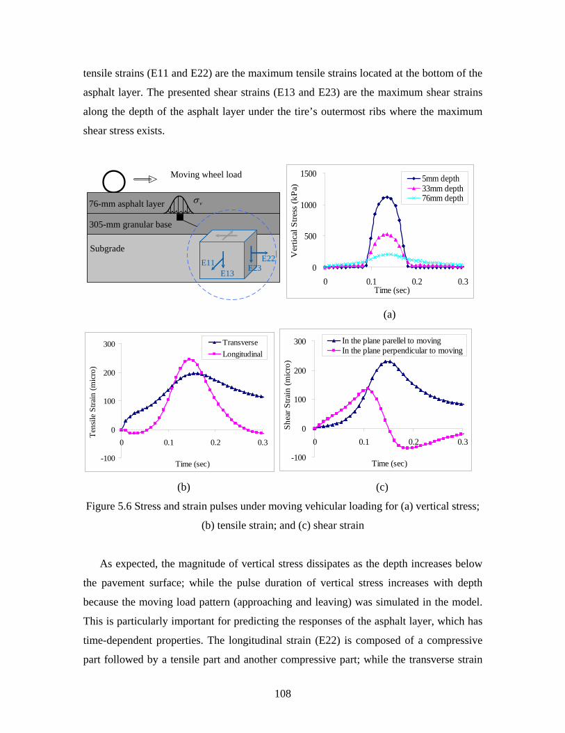
108
tensile strains (E11 and E22) are the maximum tensile strains located at the bottom of the
asphalt layer. The presented shear strains (E13 and E23) are the maximum shear strains
along the depth of the asphalt layer under the tire’s outermost ribs where the maximum
shear stress exists.
Moving wheel load
E12
E23E22E11
E13
vσ76-mm asphalt layer
305-mm granular base
Subgrade
0
500
1000
1500
0 0.1 0.2 0.3Time (sec)
Ver
tical
Stre
ss (k
Pa)
5mm depth33mm depth76mm depth
(a)
-100
0
100
200
300
0 0.1 0.2 0.3
Time (sec)
Tens
ile S
train
(mic
ro)
TransverseLongitudinal
-100
0
100
200
300
0 0.1 0.2 0.3
Time (sec)
Shea
r Stra
in (m
icro
)
In the plane parellel to movingIn the plane perpendicular to moving
(b) (c)
Figure 5.6 Stress and strain pulses under moving vehicular loading for (a) vertical stress;
(b) tensile strain; and (c) shear strain
As expected, the magnitude of vertical stress dissipates as the depth increases below
the pavement surface; while the pulse duration of vertical stress increases with depth
because the moving load pattern (approaching and leaving) was simulated in the model.
This is particularly important for predicting the responses of the asphalt layer, which has
time-dependent properties. The longitudinal strain (E22) is composed of a compressive
part followed by a tensile part and another compressive part; while the transverse strain
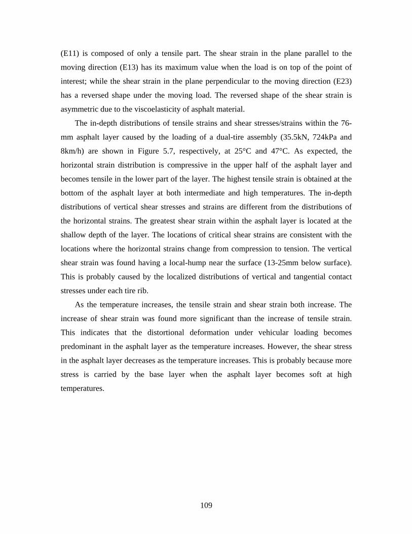
109
(E11) is composed of only a tensile part. The shear strain in the plane parallel to the
moving direction (E13) has its maximum value when the load is on top of the point of
interest; while the shear strain in the plane perpendicular to the moving direction (E23)
has a reversed shape under the moving load. The reversed shape of the shear strain is
asymmetric due to the viscoelasticity of asphalt material.
The in-depth distributions of tensile strains and shear stresses/strains within the 76-
mm asphalt layer caused by the loading of a dual-tire assembly (35.5kN, 724kPa and
8km/h) are shown in Figure 5.7, respectively, at 25°C and 47°C. As expected, the
horizontal strain distribution is compressive in the upper half of the asphalt layer and
becomes tensile in the lower part of the layer. The highest tensile strain is obtained at the
bottom of the asphalt layer at both intermediate and high temperatures. The in-depth
distributions of vertical shear stresses and strains are different from the distributions of
the horizontal strains. The greatest shear strain within the asphalt layer is located at the
shallow depth of the layer. The locations of critical shear strains are consistent with the
locations where the horizontal strains change from compression to tension. The vertical
shear strain was found having a local-hump near the surface (13-25mm below surface).
This is probably caused by the localized distributions of vertical and tangential contact
stresses under each tire rib.
As the temperature increases, the tensile strain and shear strain both increase. The
increase of shear strain was found more significant than the increase of tensile strain.
This indicates that the distortional deformation under vehicular loading becomes
predominant in the asphalt layer as the temperature increases. However, the shear stress
in the asphalt layer decreases as the temperature increases. This is probably because more
stress is carried by the base layer when the asphalt layer becomes soft at high
temperatures.
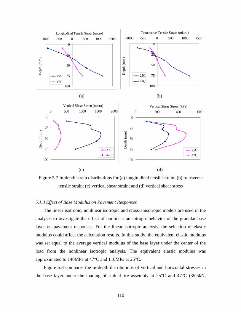
110
0
25
50
75
100
-1000 -500 0 500 1000 1500Longitudinal Tensile Strain (micro)
Dep
th (m
m)
25C47C
0
25
50
75
100
-1000 -500 0 500 1000 1500Transverse Tensile Strain (micro)
Dep
th (m
m)
25C47C
(a) (b)
0
25
50
75
100
0 500 1000 1500 2000Vertical Shear Strain (micro)
Dep
th (m
m)
25C47C
0
25
50
75
100
0 200 400 600Vertical Shear Stress (kPa)
Dep
th (m
m)
25C47C
(c) (d)
Figure 5.7 In-depth strain distributions for (a) longitudinal tensile strain; (b) transverse
tensile strain; (c) vertical shear strain; and (d) vertical shear stress
5.1.3 Effect of Base Modulus on Pavement Responses
The linear isotropic, nonlinear isotropic and cross-anisotropic models are used in the
analyses to investigate the effect of nonlinear anisotropic behavior of the granular base
layer on pavement responses. For the linear isotropic analysis, the selection of elastic
modulus could affect the calculation results. In this study, the equivalent elastic modulus
was set equal to the average vertical modulus of the base layer under the center of the
load from the nonlinear isotropic analysis. The equivalent elastic modulus was
approximated to 140MPa at 47°C and 110MPa at 25°C.
Figure 5.8 compares the in-depth distributions of vertical and horizontal stresses in
the base layer under the loading of a dual-tire assembly at 25°C and 47°C (35.5kN,
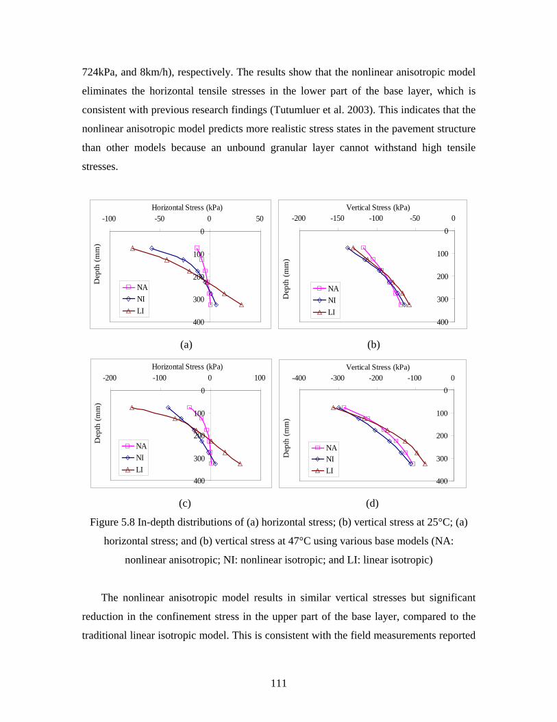
111
724kPa, and 8km/h), respectively. The results show that the nonlinear anisotropic model
eliminates the horizontal tensile stresses in the lower part of the base layer, which is
consistent with previous research findings (Tutumluer et al. 2003). This indicates that the
nonlinear anisotropic model predicts more realistic stress states in the pavement structure
than other models because an unbound granular layer cannot withstand high tensile
stresses.
0
100
200
300
400
-100 -50 0 50Horizontal Stress (kPa)
Dep
th (m
m)
NANILI
0
100
200
300
400
-200 -150 -100 -50 0Vertical Stress (kPa)
Dep
th (m
m)
NANILI
(a) (b)
0
100
200
300
400
-200 -100 0 100Horizontal Stress (kPa)
Dep
th (m
m)
NANILI
0
100
200
300
400
-400 -300 -200 -100 0Vertical Stress (kPa)
Dep
th (m
m)
NANILI
(c) (d)
Figure 5.8 In-depth distributions of (a) horizontal stress; (b) vertical stress at 25°C; (a)
horizontal stress; and (b) vertical stress at 47°C using various base models (NA:
nonlinear anisotropic; NI: nonlinear isotropic; and LI: linear isotropic)
The nonlinear anisotropic model results in similar vertical stresses but significant
reduction in the confinement stress in the upper part of the base layer, compared to the
traditional linear isotropic model. This is consistent with the field measurements reported
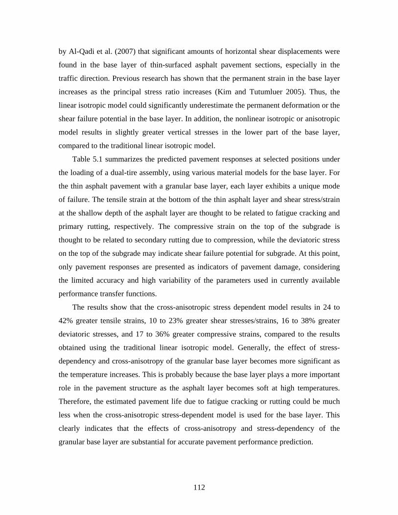
112
by Al-Qadi et al. (2007) that significant amounts of horizontal shear displacements were
found in the base layer of thin-surfaced asphalt pavement sections, especially in the
traffic direction. Previous research has shown that the permanent strain in the base layer
increases as the principal stress ratio increases (Kim and Tutumluer 2005). Thus, the
linear isotropic model could significantly underestimate the permanent deformation or the
shear failure potential in the base layer. In addition, the nonlinear isotropic or anisotropic
model results in slightly greater vertical stresses in the lower part of the base layer,
compared to the traditional linear isotropic model.
Table 5.1 summarizes the predicted pavement responses at selected positions under
the loading of a dual-tire assembly, using various material models for the base layer. For
the thin asphalt pavement with a granular base layer, each layer exhibits a unique mode
of failure. The tensile strain at the bottom of the thin asphalt layer and shear stress/strain
at the shallow depth of the asphalt layer are thought to be related to fatigue cracking and
primary rutting, respectively. The compressive strain on the top of the subgrade is
thought to be related to secondary rutting due to compression, while the deviatoric stress
on the top of the subgrade may indicate shear failure potential for subgrade. At this point,
only pavement responses are presented as indicators of pavement damage, considering
the limited accuracy and high variability of the parameters used in currently available
performance transfer functions.
The results show that the cross-anisotropic stress dependent model results in 24 to
42% greater tensile strains, 10 to 23% greater shear stresses/strains, 16 to 38% greater
deviatoric stresses, and 17 to 36% greater compressive strains, compared to the results
obtained using the traditional linear isotropic model. Generally, the effect of stress-
dependency and cross-anisotropy of the granular base layer becomes more significant as
the temperature increases. This is probably because the base layer plays a more important
role in the pavement structure as the asphalt layer becomes soft at high temperatures.
Therefore, the estimated pavement life due to fatigue cracking or rutting could be much
less when the cross-anisotropic stress-dependent model is used for the base layer. This
clearly indicates that the effects of cross-anisotropy and stress-dependency of the
granular base layer are substantial for accurate pavement performance prediction.
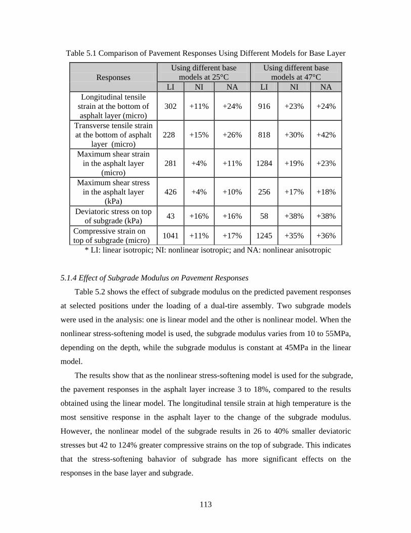
113
Table 5.1 Comparison of Pavement Responses Using Different Models for Base Layer
Responses Using different base
models at 25°C Using different base
models at 47°C LI NI NA LI NI NA
Longitudinal tensile strain at the bottom of asphalt layer (micro)
302 +11% +24% 916 +23% +24%
Transverse tensile strain at the bottom of asphalt
layer (micro) 228 +15% +26% 818 +30% +42%
Maximum shear strain in the asphalt layer
(micro) 281 +4% +11% 1284 +19% +23%
Maximum shear stress in the asphalt layer
(kPa) 426 +4% +10% 256 +17% +18%
Deviatoric stress on top of subgrade (kPa) 43 +16% +16% 58 +38% +38%
Compressive strain on top of subgrade (micro) 1041 +11% +17% 1245 +35% +36%
* LI: linear isotropic; NI: nonlinear isotropic; and NA: nonlinear anisotropic
5.1.4 Effect of Subgrade Modulus on Pavement Responses
Table 5.2 shows the effect of subgrade modulus on the predicted pavement responses
at selected positions under the loading of a dual-tire assembly. Two subgrade models
were used in the analysis: one is linear model and the other is nonlinear model. When the
nonlinear stress-softening model is used, the subgrade modulus varies from 10 to 55MPa,
depending on the depth, while the subgrade modulus is constant at 45MPa in the linear
model.
The results show that as the nonlinear stress-softening model is used for the subgrade,
the pavement responses in the asphalt layer increase 3 to 18%, compared to the results
obtained using the linear model. The longitudinal tensile strain at high temperature is the
most sensitive response in the asphalt layer to the change of the subgrade modulus.
However, the nonlinear model of the subgrade results in 26 to 40% smaller deviatoric
stresses but 42 to 124% greater compressive strains on the top of subgrade. This indicates
that the stress-softening bahavior of subgrade has more significant effects on the
responses in the base layer and subgrade.
114
Table 5.2 Comparison of Pavement Responses Using Different Models for Subgrade
Responses Using different subgrade
models at 25°C Using different subgrade
models at 47°C Linear Nonlinear Linear Nonlinear
Longitudinal tensile strain at the bottom of asphalt
layer (micro) 375 +6% 1139 +18%
Transverse tensile strain at the bottom of asphalt layer
(micro) 288 +3% 1162 +6%
Maximum shear strain in the asphalt layer (micro) 311 +4% 1573 +7%
Maximum shear stress in the asphalt layer
(kPa) 467 +3% 303 +4%
Deviatoric stress on top of subgrade (kPa) 50 -26% 77 -40%
Compressive strain on top of subgrade (micro) 1151 +42% 1678 +124%
5.2 Influence of Loading Conditions on Pavement Responses
5.2.1 Effect of 3-D Contact Stresses
To evaluate the effect of 3-D contact stresses on thin asphalt pavement responses,
two groups of analyses were conducted: one using the 3-D contact stress distribution, and
another using the uniform contact stress distribution. Table 5.3 shows the detailed
comparison between the two different contact stress distributions. The uniform contact
stress was calculated as the total load divided by the actual tire-pavement contact area.
The analyses were conducted by loading a dual-tire assembly at a speed of 8km/h under
various loads and tire inflation pressures.
Tables 5.4 and 5.5 compare the predicted pavement responses at selected positions
using the uniform and 3-D contact stress distributions, respectively, under various loads
and tire inflation pressures. The results show that the differences in response between two
contact stress distributions depend on the type of response, the asphalt mixture stiffness,
and the applied load and tire pressure.
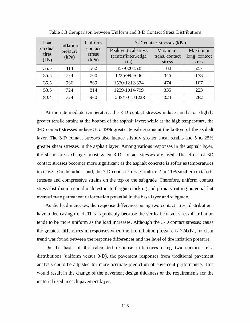
115
Table 5.3 Comparison between Uniform and 3-D Contact Stress Distributions
Load on dual
tires (kN)
Inflation pressure
(kPa)
Uniform contact stress (kPa)
3-D contact stresses (kPa) Peak vertical stress (center/inter./edge
rib)
Maximum trans. contact
stress
Maximum long. contact
stress 35.5 414 562 857/626/528 180 257 35.5 724 700 1235/995/606 346 173 35.5 966 869 1530/1212/674 474 107 53.6 724 814 1239/1014/799 335 223 80.4 724 960 1248/1017/1233 324 262
At the intermediate temperature, the 3-D contact stresses induce similar or slightly
greater tensile strains at the bottom of the asphalt layer; while at the high temperature, the
3-D contact stresses induce 3 to 19% greater tensile strains at the bottom of the asphalt
layer. The 3-D contact stresses also induce slightly greater shear strains and 5 to 25%
greater shear stresses in the asphalt layer. Among various responses in the asphalt layer,
the shear stress changes most when 3-D contact stresses are used. The effect of 3D
contact stresses becomes more significant as the asphalt concrete is softer as temperatures
increase. On the other hand, the 3-D contact stresses induce 2 to 11% smaller deviatoric
stresses and compressive strains on the top of the subgrade. Therefore, uniform contact
stress distribution could underestimate fatigue cracking and primary rutting potential but
overestimate permanent deformation potential in the base layer and subgrade.
As the load increases, the response differences using two contact stress distributions
have a decreasing trend. This is probably because the vertical contact stress distribution
tends to be more uniform as the load increases. Although the 3-D contact stresses cause
the greatest differences in responses when the tire inflation pressure is 724kPa, no clear
trend was found between the response differences and the level of tire inflation pressure.
On the basis of the calculated response differences using two contact stress
distributions (uniform versus 3-D), the pavement responses from traditional pavement
analysis could be adjusted for more accurate prediction of pavement performance. This
would result in the change of the pavement design thickness or the requirements for the
material used in each pavement layer.
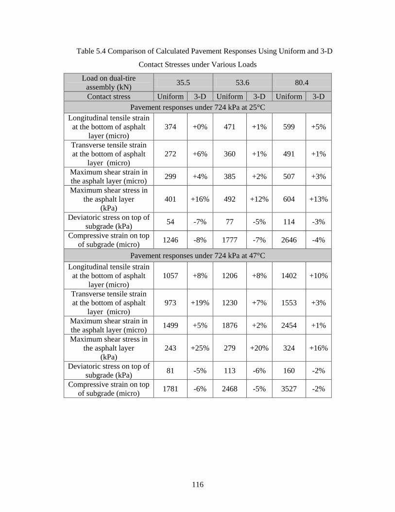
116
Table 5.4 Comparison of Calculated Pavement Responses Using Uniform and 3-D
Contact Stresses under Various Loads
Load on dual-tire assembly (kN) 35.5 53.6 80.4
Contact stress Uniform 3-D Uniform 3-D Uniform 3-D Pavement responses under 724 kPa at 25°C
Longitudinal tensile strain at the bottom of asphalt
layer (micro) 374 +0% 471 +1% 599 +5%
Transverse tensile strain at the bottom of asphalt
layer (micro) 272 +6% 360 +1% 491 +1%
Maximum shear strain in the asphalt layer (micro) 299 +4% 385 +2% 507 +3%
Maximum shear stress in the asphalt layer
(kPa) 401 +16% 492 +12% 604 +13%
Deviatoric stress on top of subgrade (kPa) 54 -7% 77 -5% 114 -3%
Compressive strain on top of subgrade (micro) 1246 -8% 1777 -7% 2646 -4%
Pavement responses under 724 kPa at 47°C Longitudinal tensile strain
at the bottom of asphalt layer (micro)
1057 +8% 1206 +8% 1402 +10%
Transverse tensile strain at the bottom of asphalt
layer (micro) 973 +19% 1230 +7% 1553 +3%
Maximum shear strain in the asphalt layer (micro) 1499 +5% 1876 +2% 2454 +1%
Maximum shear stress in the asphalt layer
(kPa) 243 +25% 279 +20% 324 +16%
Deviatoric stress on top of subgrade (kPa) 81 -5% 113 -6% 160 -2%
Compressive strain on top of subgrade (micro) 1781 -6% 2468 -5% 3527 -2%
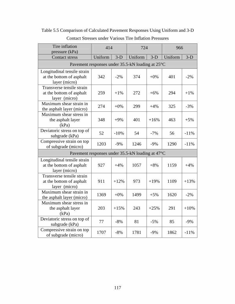
117
Table 5.5 Comparison of Calculated Pavement Responses Using Uniform and 3-D
Contact Stresses under Various Tire Inflation Pressures
Tire inflation pressure (kPa)
414 724 966
Contact stress Uniform 3-D Uniform 3-D Uniform 3-D Pavement responses under 35.5-kN loading at 25°C
Longitudinal tensile strain at the bottom of asphalt
layer (micro) 342 -2% 374 +0% 401 -2%
Transverse tensile strain at the bottom of asphalt
layer (micro) 259 +1% 272 +6% 294 +1%
Maximum shear strain in the asphalt layer (micro) 274 +0% 299 +4% 325 -3%
Maximum shear stress in the asphalt layer
(kPa) 348 +9% 401 +16% 463 +5%
Deviatoric stress on top of subgrade (kPa) 52 -10% 54 -7% 56 -11%
Compressive strain on top of subgrade (micro) 1203 -9% 1246 -9% 1290 -11%
Pavement responses under 35.5-kN loading at 47°C Longitudinal tensile strain
at the bottom of asphalt layer (micro)
927 +4% 1057 +8% 1159 +4%
Transverse tensile strain at the bottom of asphalt
layer (micro) 911 +12% 973 +19% 1109 +13%
Maximum shear strain in the asphalt layer (micro) 1369 +0% 1499 +5% 1620 -2%
Maximum shear stress in the asphalt layer
(kPa) 203 +15% 243 +25% 291 +10%
Deviatoric stress on top of subgrade (kPa) 77 -8% 81 -5% 85 -9%
Compressive strain on top of subgrade (micro) 1707 -8% 1781 -9% 1862 -11%
118
5.2.2 Effect of Wheel Load and Tire Pressure
Tables 5.6 and 5.7 compare the predicted pavement responses at selected positions
using the 3-D contact stresses under various wheel loads and tire inflation pressures. As
expected, the heavier load or higher tire inflation pressure induces greater pavement
responses. The heavy load mainly causes the increase of responses in the subgrade, while
the effect of tire inflation pressure is more significant for the responses in the asphalt
layer. As the load increases, the vertical contact stress distribution tends to be more
uniform and the tire contact area increases significantly. On the other hand, when the tire
inflation pressure increases, the high vertical contact stress tends to concentrate in the
central region of the tire contact area. This indicates that the responses in the upper part
of the pavement are more affected by the localized tire-pavement contact stress
distributions. However, deeper in the pavement, the responses are mainly controlled by
the total load and contact area.
The results show that the effect of tire inflation pressure is more related to the shear
stress in the asphalt layer, compared to other pavement responses. This is probably
because, under high tire inflation pressure, the high vertical contact stress in the central
region of the tire contact area and the high tangential contact stress could cause more
shear flow at tire edges under low confinements. Interestingly, it was found that the load
effect is more significant at intermediate temperatures; while the tire inflation pressure
effect is more significant at high temperatures. This indicates that the shear-resistant
asphalt mixture is desired when the truck tire pressure is high in the regions with warm
climates, while the axle weight limit should be enforced during spring seasons on low-
volume roads in order to minimize pavement damage.
119
Table 5.6 Effect of Loads on Calculated Pavement Responses
Pavement responses under 724kPa (Dual-tire Assembly)
Temperature At 25°C At 47°C Load on dual tires (kN) 35.5 53.6 80.4 35.5 53.6 80.4
Longitudinal tensile strain at the bottom of asphalt layer (micro) 375 +27% +67% 1139 +15% +35%
Transverse tensile strain at the bottom of asphalt layer (micro) 288 +26% +72% 1162 +14% +38%
Maximum shear strain in the asphalt layer (micro) 311 +26% +68% 1573 +22% +58%
Maximum shear stress in the asphalt layer
(kPa) 467 +18% +46% 303 +11% +24%
Deviatoric stress on top of subgrade (kPa) 50 +42% +122% 77 +38% +104%
Compressive strain on top of subgrade (micro) 1151 +44% +121% 1678 +40% +106%
Table 5.7 Effect of Inflation Pressure on Calculated Pavement Responses
Pavement responses under 35.5kN (Dual-tire Assembly)
Temperature At 25°C At 47°C Pressure (kPa) 414 724 966 414 724 966
Longitudinal tensile strain at the bottom of asphalt layer (micro) 335 +12% +14% 960 +19% +25%
Transverse tensile strain at the bottom of asphalt layer (micro) 261 +10% +14% 1020 +14% +23%
Maximum shear strain in the asphalt layer (micro) 274 +14% +15% 1373 +15% +16%
Maximum shear stress in the asphalt layer
(kPa) 378 +24% +28% 234 +29% +37%
Deviatoric stress on top of subgrade (kPa) 47 +6% +6% 71 +8% +8%
Compressive strain on top of subgrade (micro) 1090 +4% +6% 1575 +3% +2%
It is noted that the pavement responses increase proportionally as the load increases,
while the response changes as the tire pressure increases from 414kPa to 724kPa are
more significant than the response changes as the tire pressure increases from 724kPa to
966kPa. This is probably due to the variation of localized tire contact stresses as the tire
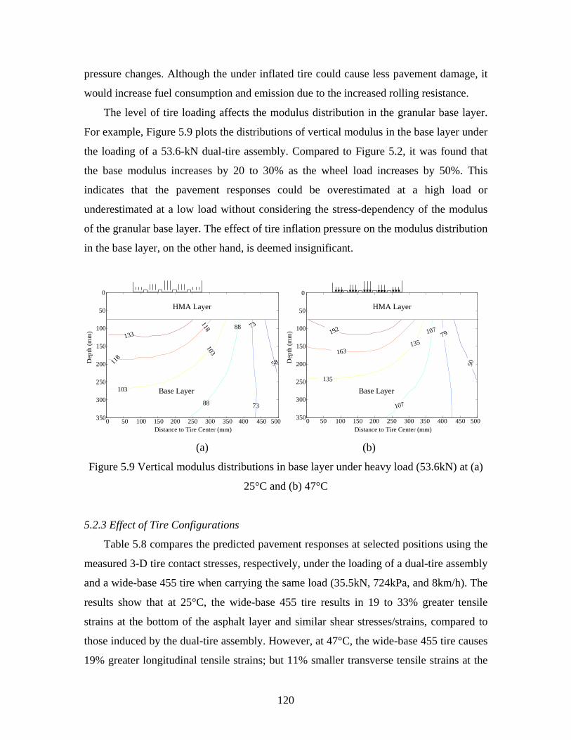
120
pressure changes. Although the under inflated tire could cause less pavement damage, it
would increase fuel consumption and emission due to the increased rolling resistance.
The level of tire loading affects the modulus distribution in the granular base layer.
For example, Figure 5.9 plots the distributions of vertical modulus in the base layer under
the loading of a 53.6-kN dual-tire assembly. Compared to Figure 5.2, it was found that
the base modulus increases by 20 to 30% as the wheel load increases by 50%. This
indicates that the pavement responses could be overestimated at a high load or
underestimated at a low load without considering the stress-dependency of the modulus
of the granular base layer. The effect of tire inflation pressure on the modulus distribution
in the base layer, on the other hand, is deemed insignificant.
58
73
73
88
88
103
103
11811
8
133
0 50 100 150 200 250 300 350 400 450 500
0
50
100
150
200
250
300
350
HMA Layer
Distance to Tire Center (mm)
Dep
th (m
m)
Base Layer
50
79
107
107
135
135
163
192
0 50 100 150 200 250 300 350 400 450 500
0
50
100
150
200
250
300
350
HMA Layer
Distance to Tire Center (mm)
Dep
th (m
m)
Base Layer
(a) (b)
Figure 5.9 Vertical modulus distributions in base layer under heavy load (53.6kN) at (a)
25°C and (b) 47°C
5.2.3 Effect of Tire Configurations
Table 5.8 compares the predicted pavement responses at selected positions using the
measured 3-D tire contact stresses, respectively, under the loading of a dual-tire assembly
and a wide-base 455 tire when carrying the same load (35.5kN, 724kPa, and 8km/h). The
results show that at 25°C, the wide-base 455 tire results in 19 to 33% greater tensile
strains at the bottom of the asphalt layer and similar shear stresses/strains, compared to
those induced by the dual-tire assembly. However, at 47°C, the wide-base 455 tire causes
19% greater longitudinal tensile strains; but 11% smaller transverse tensile strains at the
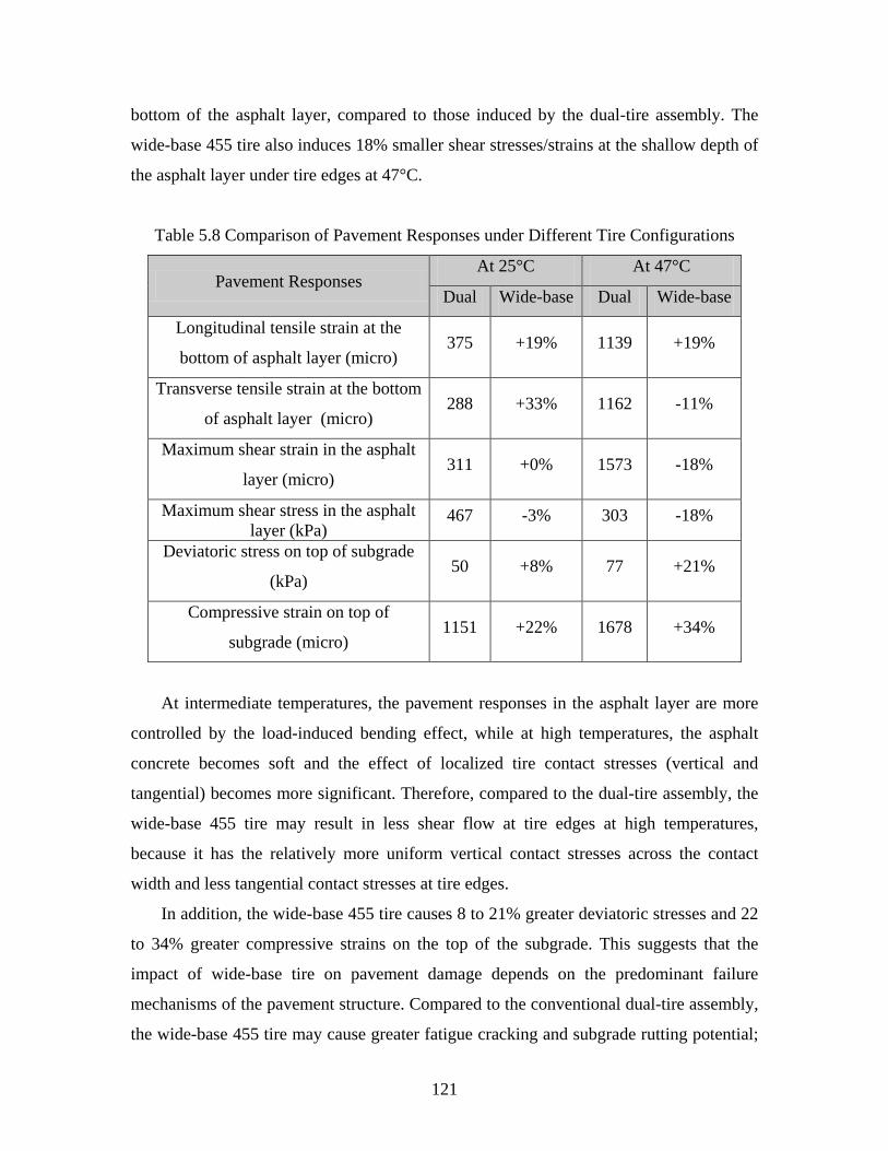
121
bottom of the asphalt layer, compared to those induced by the dual-tire assembly. The
wide-base 455 tire also induces 18% smaller shear stresses/strains at the shallow depth of
the asphalt layer under tire edges at 47°C.
Table 5.8 Comparison of Pavement Responses under Different Tire Configurations
Pavement Responses At 25°C At 47°C
Dual Wide-base Dual Wide-base
Longitudinal tensile strain at the
bottom of asphalt layer (micro) 375 +19% 1139 +19%
Transverse tensile strain at the bottom
of asphalt layer (micro) 288 +33% 1162 -11%
Maximum shear strain in the asphalt
layer (micro) 311 +0% 1573 -18%
Maximum shear stress in the asphalt layer (kPa)
467 -3% 303 -18%
Deviatoric stress on top of subgrade
(kPa) 50 +8% 77 +21%
Compressive strain on top of
subgrade (micro) 1151 +22% 1678 +34%
At intermediate temperatures, the pavement responses in the asphalt layer are more
controlled by the load-induced bending effect, while at high temperatures, the asphalt
concrete becomes soft and the effect of localized tire contact stresses (vertical and
tangential) becomes more significant. Therefore, compared to the dual-tire assembly, the
wide-base 455 tire may result in less shear flow at tire edges at high temperatures,
because it has the relatively more uniform vertical contact stresses across the contact
width and less tangential contact stresses at tire edges.
In addition, the wide-base 455 tire causes 8 to 21% greater deviatoric stresses and 22
to 34% greater compressive strains on the top of the subgrade. This suggests that the
impact of wide-base tire on pavement damage depends on the predominant failure
mechanisms of the pavement structure. Compared to the conventional dual-tire assembly,
the wide-base 455 tire may cause greater fatigue cracking and subgrade rutting potential;
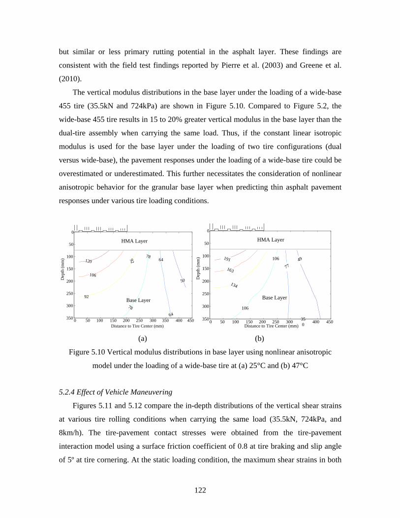
122
but similar or less primary rutting potential in the asphalt layer. These findings are
consistent with the field test findings reported by Pierre et al. (2003) and Greene et al.
(2010).
The vertical modulus distributions in the base layer under the loading of a wide-base
455 tire (35.5kN and 724kPa) are shown in Figure 5.10. Compared to Figure 5.2, the
wide-base 455 tire results in 15 to 20% greater vertical modulus in the base layer than the
dual-tire assembly when carrying the same load. Thus, if the constant linear isotropic
modulus is used for the base layer under the loading of two tire configurations (dual
versus wide-base), the pavement responses under the loading of a wide-base tire could be
overestimated or underestimated. This further necessitates the consideration of nonlinear
anisotropic behavior for the granular base layer when predicting thin asphalt pavement
responses under various tire loading conditions.
50
64
64
78
7892
92
106
120
0 50 100 150 200 250 300 350 400 450
0
50
100
150
200
250
300
350
HMA Layer
Base Layer
Distance to Tire Center (mm)
Dep
th (m
m) 49
77
106
106
134
163
191
0 50 100 150 200 250 300 350 400 450
0
50
100
150
200
250
300
350
HMA Layer
Base Layer
Distance to Tire Center (mm)
Dep
th (m
m)
(a) (b)
Figure 5.10 Vertical modulus distributions in base layer using nonlinear anisotropic
model under the loading of a wide-base tire at (a) 25°C and (b) 47°C
5.2.4 Effect of Vehicle Maneuvering
Figures 5.11 and 5.12 compare the in-depth distributions of the vertical shear strains
at various tire rolling conditions when carrying the same load (35.5kN, 724kPa, and
8km/h). The tire-pavement contact stresses were obtained from the tire-pavement
interaction model using a surface friction coefficient of 0.8 at tire braking and slip angle
of 5º at tire cornering. At the static loading condition, the maximum shear strains in both
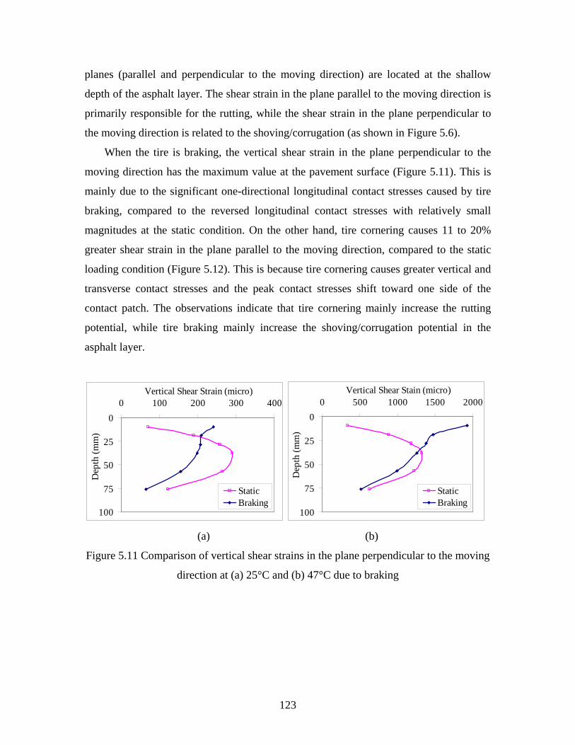
123
planes (parallel and perpendicular to the moving direction) are located at the shallow
depth of the asphalt layer. The shear strain in the plane parallel to the moving direction is
primarily responsible for the rutting, while the shear strain in the plane perpendicular to
the moving direction is related to the shoving/corrugation (as shown in Figure 5.6).
When the tire is braking, the vertical shear strain in the plane perpendicular to the
moving direction has the maximum value at the pavement surface (Figure 5.11). This is
mainly due to the significant one-directional longitudinal contact stresses caused by tire
braking, compared to the reversed longitudinal contact stresses with relatively small
magnitudes at the static condition. On the other hand, tire cornering causes 11 to 20%
greater shear strain in the plane parallel to the moving direction, compared to the static
loading condition (Figure 5.12). This is because tire cornering causes greater vertical and
transverse contact stresses and the peak contact stresses shift toward one side of the
contact patch. The observations indicate that tire cornering mainly increase the rutting
potential, while tire braking mainly increase the shoving/corrugation potential in the
asphalt layer.
0
25
50
75
100
0 100 200 300 400Vertical Shear Strain (micro)
Dep
th (m
m)
StaticBraking
0
25
50
75
100
0 500 1000 1500 2000Vertical Shear Stain (micro)
Dep
th (m
m)
StaticBraking
(a) (b)
Figure 5.11 Comparison of vertical shear strains in the plane perpendicular to the moving
direction at (a) 25°C and (b) 47°C due to braking
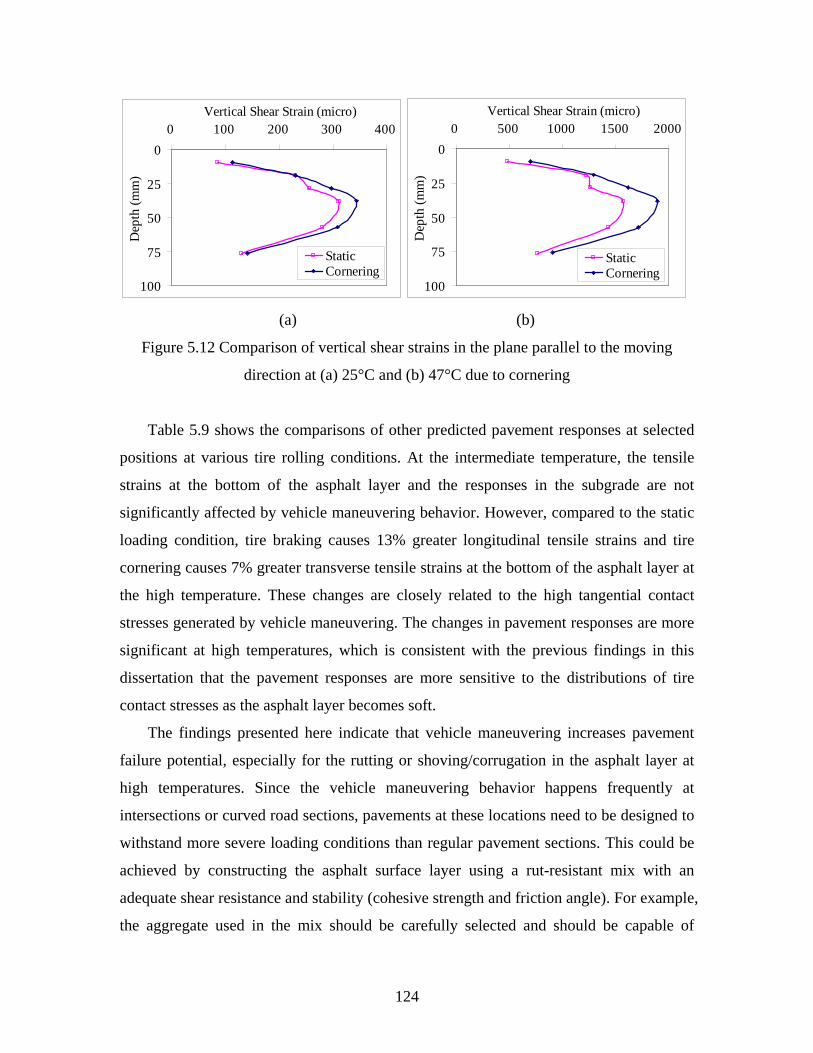
124
0
25
50
75
100
0 100 200 300 400Vertical Shear Strain (micro)
Dep
th (m
m)
StaticCornering
0
25
50
75
100
0 500 1000 1500 2000Vertical Shear Strain (micro)
Dep
th (m
m)
StaticCornering
(a) (b)
Figure 5.12 Comparison of vertical shear strains in the plane parallel to the moving
direction at (a) 25°C and (b) 47°C due to cornering
Table 5.9 shows the comparisons of other predicted pavement responses at selected
positions at various tire rolling conditions. At the intermediate temperature, the tensile
strains at the bottom of the asphalt layer and the responses in the subgrade are not
significantly affected by vehicle maneuvering behavior. However, compared to the static
loading condition, tire braking causes 13% greater longitudinal tensile strains and tire
cornering causes 7% greater transverse tensile strains at the bottom of the asphalt layer at
the high temperature. These changes are closely related to the high tangential contact
stresses generated by vehicle maneuvering. The changes in pavement responses are more
significant at high temperatures, which is consistent with the previous findings in this
dissertation that the pavement responses are more sensitive to the distributions of tire
contact stresses as the asphalt layer becomes soft.
The findings presented here indicate that vehicle maneuvering increases pavement
failure potential, especially for the rutting or shoving/corrugation in the asphalt layer at
high temperatures. Since the vehicle maneuvering behavior happens frequently at
intersections or curved road sections, pavements at these locations need to be designed to
withstand more severe loading conditions than regular pavement sections. This could be
achieved by constructing the asphalt surface layer using a rut-resistant mix with an
adequate shear resistance and stability (cohesive strength and friction angle). For example,
the aggregate used in the mix should be carefully selected and should be capable of
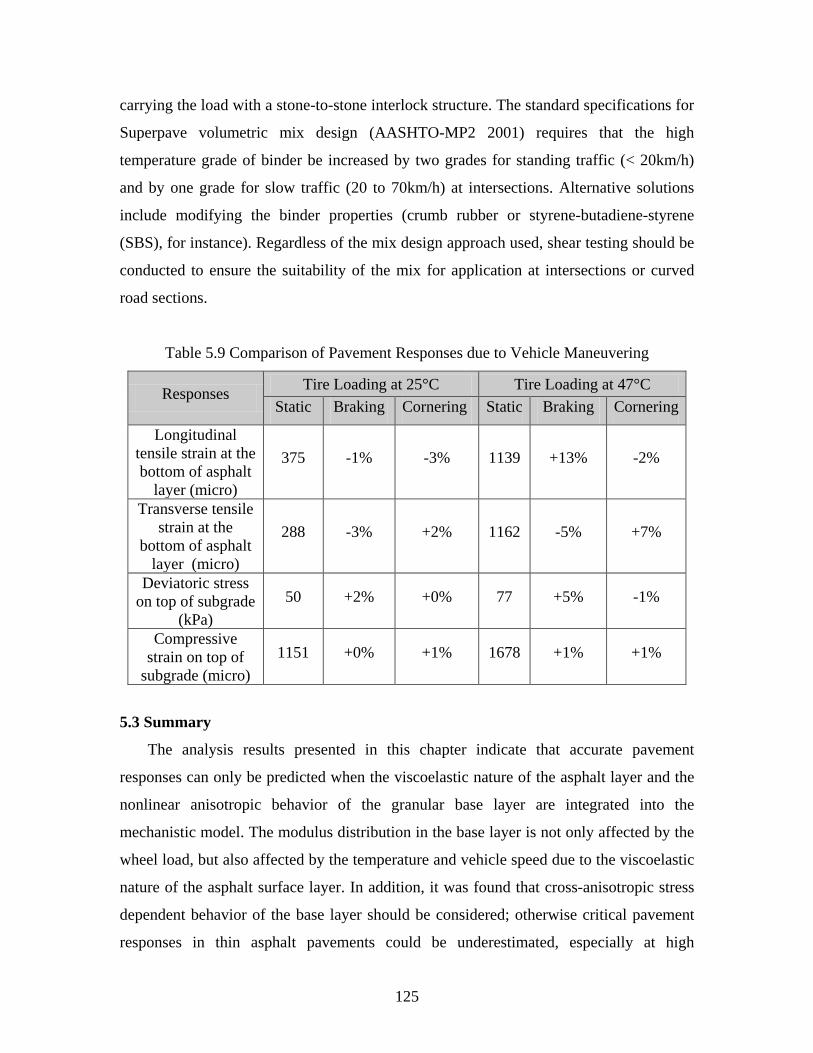
125
carrying the load with a stone-to-stone interlock structure. The standard specifications for
Superpave volumetric mix design (AASHTO-MP2 2001) requires that the high
temperature grade of binder be increased by two grades for standing traffic (< 20km/h)
and by one grade for slow traffic (20 to 70km/h) at intersections. Alternative solutions
include modifying the binder properties (crumb rubber or styrene-butadiene-styrene
(SBS), for instance). Regardless of the mix design approach used, shear testing should be
conducted to ensure the suitability of the mix for application at intersections or curved
road sections.
Table 5.9 Comparison of Pavement Responses due to Vehicle Maneuvering
Responses Tire Loading at 25°C Tire Loading at 47°C Static Braking Cornering Static Braking Cornering
Longitudinal tensile strain at the bottom of asphalt
layer (micro)
375 -1% -3% 1139 +13% -2%
Transverse tensile strain at the
bottom of asphalt layer (micro)
288 -3% +2% 1162 -5% +7%
Deviatoric stress on top of subgrade
(kPa) 50 +2% +0% 77 +5% -1%
Compressive strain on top of
subgrade (micro) 1151 +0% +1% 1678 +1% +1%
5.3 Summary
The analysis results presented in this chapter indicate that accurate pavement
responses can only be predicted when the viscoelastic nature of the asphalt layer and the
nonlinear anisotropic behavior of the granular base layer are integrated into the
mechanistic model. The modulus distribution in the base layer is not only affected by the
wheel load, but also affected by the temperature and vehicle speed due to the viscoelastic
nature of the asphalt surface layer. In addition, it was found that cross-anisotropic stress
dependent behavior of the base layer should be considered; otherwise critical pavement
responses in thin asphalt pavements could be underestimated, especially at high
126
temperatures. However, the stress-softening behavior of subgrade mainly affects the
responses in the subgrade.
The critical pavement responses in thin asphalt pavements at various tire loading and
rolling conditions were analyzed. It is concluded that compared to the uniform contact
stress distribution, the 3-D tire contact stresses cause greater fatigue cracking and primary
rutting potential but less failure potential in the subgrade. The calculation of pavement
responses are affected by the vehicle loading (wheel load and tire inflation pressure), tire
configuration (dual-tire assembly and wide-base tire), and vehicle maneuvering behavior
(braking/acceleration and cornering). Generally, the pavement responses are more
sensitive to the distributions of tire contact stresses as the asphalt layer becomes soft at
high temperatures.
127
CHAPTER 6 NEAR-SURFACE FAILURE POTENTIAL OF THICK ASPHALT
PAVEMENT
6.1 Near-Surface Strain Responses in Thick Asphalt Pavement
Long-lasting or perpetual pavement is designed to prevent cracks from initiating at
the bottom of the asphalt layer by increasing the asphalt layer thickness or placing a
binder-rich layer as the lowest asphalt layer (Newcomb 2001). However, surface-related
cracking has recently been observed at the surface or near-surface of thick asphalt
pavements or overlays as a premature failure. Therefore, it is important to examine the
pavement responses that are related to the failure at the pavement near-surface.
Table 6.1 summarizes the contributing load-related parameters to the surface-initiated
cracking that were investigated in the literature. It shows that both the tensile and shear
stresses/strains are thought to be related to the near-surface failure, although the analysis
approaches, contact stress assumptions, and material models differ in the literature.
Table 6.1 Mechanisms of Surface-Initiated Cracking in the Literature
Literature Contributing parameters to surface-
initiated cracking
Merrill (2000) and Thom (2003) Tensile strain at tire edge
Groenendijk (1998); Myers et al. (1998);
Svasdisant (2002); Soon et al. (2003)
Surface tensile stress around tire edge
(plus aging and thermal stress)
Bensalem et al. (2000); Yoo and Al-Qadi
(2008); and Al-Qadi et al. (2008) Load-induced shear strain at tire edge
CROW (1990); Wang and Al-Qadi (2009) Octahedral shear stress or distortional
energy
In this chapter, the thick asphalt pavement section with a 254-mm-thick asphalt layer,
described in Chapter 4, is used in the analysis. Figure 6.1 shows the strain distributions
along the tire width at the pavement near-surface (13-25mm below surface) under the
loading of a dual-tire assembly (35.5kN, 724kPa, 8km/h, and 25°C), respectively, for the
maximum tensile strain and the vertical shear strain. The greatest surface tensile strains

128
were found located at some distance away from tire edges, especially the inner tire edges.
However, the magnitudes of the surface tensile strains are small compared to the possible
endurance limit of asphalt concrete (70-100micro) for fatigue cracking (Carpenter et al.
2003). This indicates that the surface-initiated cracking cannot be induced by surface
tensile strains only and the effect of shear strains cannot be neglected. On the other hand,
the calculated near-surface shear strains are greater than the surface tensile strains and
show a fluctuating pattern under tire ribs and grooves. The maximum near-surface shear
strain was found not under the edge ribs, but under the inner ribs, where the maximum
transverse tire-pavement contact stress exists.
-40
-20
0
20
40
60
80
-600 -400 -200 0 200 400 600
Distance to Tire Center (mm)
Nea
r-Su
rfac
e Te
nsile
Stra
in (m
icro
)
Tire Tire
-40
-20
0
20
40
60
80
-600 -400 -200 0 200 400 600
Distance to Tire Center (mm)
Nea
r-Su
rfac
e Te
nsile
Stra
in (m
icro
)
Tire TireTire Tire
-200
-100
0
100
200
-600 -400 -200 0 200 400 600
Distance to Tire Center (mm)
Nea
r-Su
rfac
e Sh
ear S
train
(mic
ro)
Tire Tire
-200
-100
0
100
200
-600 -400 -200 0 200 400 600
Distance to Tire Center (mm)
Nea
r-Su
rfac
e Sh
ear S
train
(mic
ro)
TireTire TireTire
(a) (b)
Figure 6.1 Transverse distributions of (a) maximum tensile strains; and (b) vertical shear
strains at the pavement near-surface
Figures 6.2 and 6.3 compare the transverse distributions of tensile and shear strains at
the pavement near-surface under various tire loading conditions (35.5kN, 724kPa, 8km/h,
and 25°C). Compared to the uniform contact stress distribution, the 3-D contact stresses
induce greater tensile and shear strains under tire ribs, but similar tensile and shear strains
at the vicinity of tire edges (Figure 6.2). Compared to the dual-tire assembly, the wide-
base 455 tire induces smaller tensile and shear strains at the pavement near-surface
(Figure 6.3). This indicates that the strain responses at the pavement near-surface are
affected by the localized tire-pavement contact stress distributions.
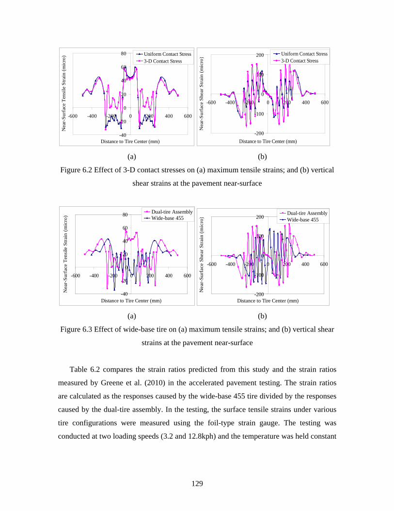
129
-40
-20
0
20
40
60
80
-600 -400 -200 0 200 400 600
Distance to Tire Center (mm)
Nea
r-Su
rfac
e Te
nsile
Stra
in (m
icro
) Uniform Contact Stress3-D Contact Stress
-200
-100
0
100
200
-600 -400 -200 0 200 400 600
Distance to Tire Center (mm)
Nea
r-Su
rfac
e Sh
ear S
trai
n (m
icro
) Uniform Contact Stress3-D Contact Stress
(a) (b)
Figure 6.2 Effect of 3-D contact stresses on (a) maximum tensile strains; and (b) vertical
shear strains at the pavement near-surface
-40
-20
0
20
40
60
80
-600 -400 -200 0 200 400 600
Distance to Tire Center (mm)
Nea
r-Su
rfac
e Te
nsile
Stra
in (m
icro
)
Dual-tire AssemblyWide-base 455
-200
-100
0
100
200
-600 -400 -200 0 200 400 600
Distance to Tire Center (mm)
Nea
r-Su
rfac
e Sh
ear S
train
(mic
ro)
Dual-tire AssemblyWide-base 455
(a) (b)
Figure 6.3 Effect of wide-base tire on (a) maximum tensile strains; and (b) vertical shear
strains at the pavement near-surface
Table 6.2 compares the strain ratios predicted from this study and the strain ratios
measured by Greene et al. (2010) in the accelerated pavement testing. The strain ratios
are calculated as the responses caused by the wide-base 455 tire divided by the responses
caused by the dual-tire assembly. In the testing, the surface tensile strains under various
tire configurations were measured using the foil-type strain gauge. The testing was
conducted at two loading speeds (3.2 and 12.8kph) and the temperature was held constant
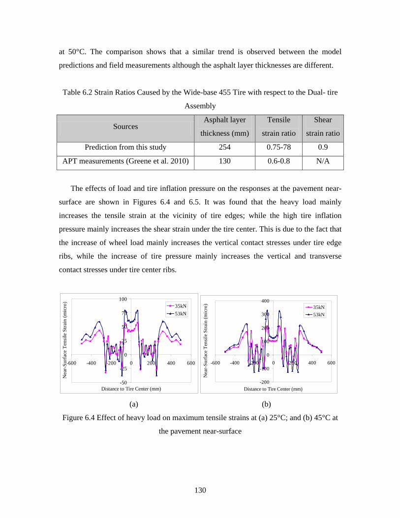
130
at 50°C. The comparison shows that a similar trend is observed between the model
predictions and field measurements although the asphalt layer thicknesses are different.
Table 6.2 Strain Ratios Caused by the Wide-base 455 Tire with respect to the Dual- tire
Assembly
Sources Asphalt layer
thickness (mm)
Tensile
strain ratio
Shear
strain ratio
Prediction from this study 254 0.75-78 0.9
APT measurements (Greene et al. 2010) 130 0.6-0.8 N/A
The effects of load and tire inflation pressure on the responses at the pavement near-
surface are shown in Figures 6.4 and 6.5. It was found that the heavy load mainly
increases the tensile strain at the vicinity of tire edges; while the high tire inflation
pressure mainly increases the shear strain under the tire center. This is due to the fact that
the increase of wheel load mainly increases the vertical contact stresses under tire edge
ribs, while the increase of tire pressure mainly increases the vertical and transverse
contact stresses under tire center ribs.
-50
-25
0
25
50
75
100
-600 -400 -200 0 200 400 600
Distance to Tire Center (mm)
Nea
r-Su
rfac
e Te
nsile
Stra
in (m
icro
)
35kN53kN
-200
-100
0
100
200
300
400
-600 -400 -200 0 200 400 600
Distance to Tire Center (mm)
Nea
r-Su
rfac
e Te
nsile
Stra
in (m
icro
)
35kN53kN
(a) (b)
Figure 6.4 Effect of heavy load on maximum tensile strains at (a) 25°C; and (b) 45°C at
the pavement near-surface
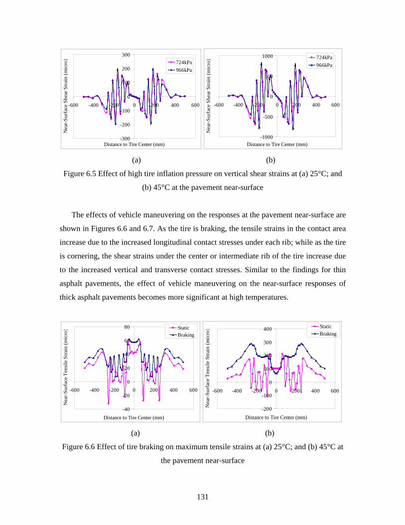
131
-300
-200
-100
0
100
200
300
-600 -400 -200 0 200 400 600
Distance to Tire Center (mm)
Nea
r-Su
rfac
e Sh
ear S
train
(mic
ro) 724kPa
966kPa
-1000
-500
0
500
1000
-600 -400 -200 0 200 400 600
Distance to Tire Center (mm)
Nea
r-Su
rfac
e Sh
ear S
train
(mic
ro) 724kPa
966kPa
(a) (b)
Figure 6.5 Effect of high tire inflation pressure on vertical shear strains at (a) 25°C; and
(b) 45°C at the pavement near-surface
The effects of vehicle maneuvering on the responses at the pavement near-surface are
shown in Figures 6.6 and 6.7. As the tire is braking, the tensile strains in the contact area
increase due to the increased longitudinal contact stresses under each rib; while as the tire
is cornering, the shear strains under the center or intermediate rib of the tire increase due
to the increased vertical and transverse contact stresses. Similar to the findings for thin
asphalt pavements, the effect of vehicle maneuvering on the near-surface responses of
thick asphalt pavements becomes more significant at high temperatures.
-40
-20
0
20
40
60
80
-600 -400 -200 0 200 400 600
Distance to Tire Center (mm)
Nea
r-Su
rfac
e Te
nsile
Stra
in (m
icro
) StaticBraking
-200
-100
0
100
200
300
400
-600 -400 -200 0 200 400 600
Distance to Tire Center (mm)
Nea
r-Su
rfac
e Te
nsile
Stra
in (m
icro
) StaticBraking
(a) (b)
Figure 6.6 Effect of tire braking on maximum tensile strains at (a) 25°C; and (b) 45°C at
the pavement near-surface
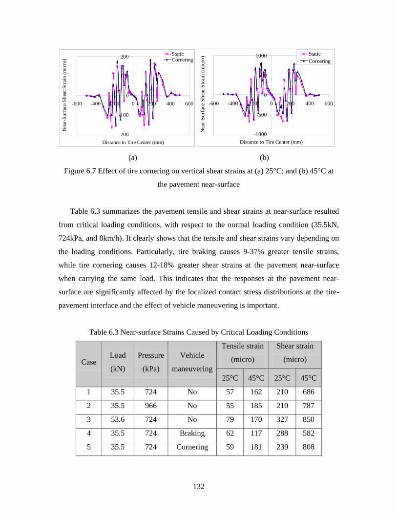
132
-200
-100
0
100
200
-600 -400 -200 0 200 400 600
Distance to Tire Center (mm)
Nea
r-Su
rfac
e Sh
ear S
train
(mic
ro)
StaticCornering
-1000
-500
0
500
1000
-600 -400 -200 0 200 400 600
Distance to Tire Center (mm)
Nea
r-Su
rfac
e Sh
ear S
train
(mic
ro) Static
Cornering
(a) (b)
Figure 6.7 Effect of tire cornering on vertical shear strains at (a) 25°C; and (b) 45°C at
the pavement near-surface
Table 6.3 summarizes the pavement tensile and shear strains at near-surface resulted
from critical loading conditions, with respect to the normal loading condition (35.5kN,
724kPa, and 8km/h). It clearly shows that the tensile and shear strains vary depending on
the loading conditions. Particularly, tire braking causes 9-37% greater tensile strains,
while tire cornering causes 12-18% greater shear strains at the pavement near-surface
when carrying the same load. This indicates that the responses at the pavement near-
surface are significantly affected by the localized contact stress distributions at the tire-
pavement interface and the effect of vehicle maneuvering is important.
Table 6.3 Near-surface Strains Caused by Critical Loading Conditions
Case Load
(kN)
Pressure
(kPa)
Vehicle
maneuvering
Tensile strain
(micro)
Shear strain
(micro)
25°C 45°C 25°C 45°C
1 35.5 724 No 57 162 210 686
2 35.5 966 No 55 185 210 787
3 53.6 724 No 79 170 327 850
4 35.5 724 Braking 62 117 288 582
5 35.5 724 Cornering 59 181 239 808
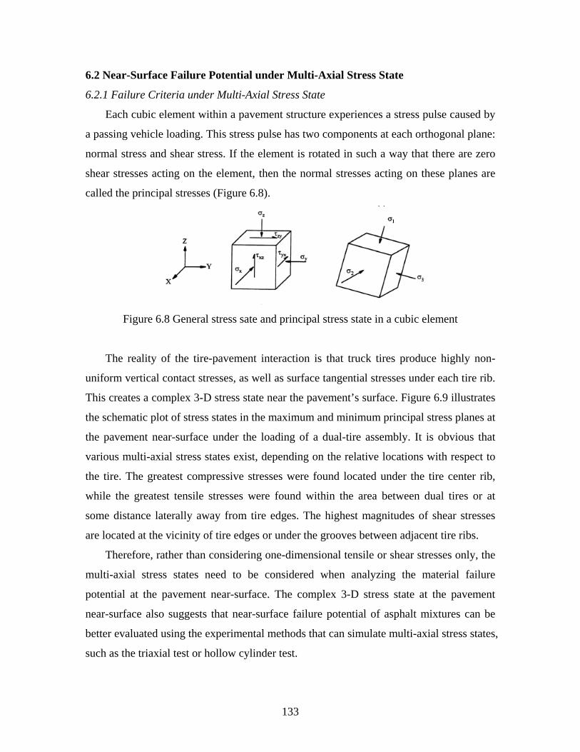
133
6.2 Near-Surface Failure Potential under Multi-Axial Stress State
6.2.1 Failure Criteria under Multi-Axial Stress State
Each cubic element within a pavement structure experiences a stress pulse caused by
a passing vehicle loading. This stress pulse has two components at each orthogonal plane:
normal stress and shear stress. If the element is rotated in such a way that there are zero
shear stresses acting on the element, then the normal stresses acting on these planes are
called the principal stresses (Figure 6.8).
Figure 6.8 General stress sate and principal stress state in a cubic element
The reality of the tire-pavement interaction is that truck tires produce highly non-
uniform vertical contact stresses, as well as surface tangential stresses under each tire rib.
This creates a complex 3-D stress state near the pavement’s surface. Figure 6.9 illustrates
the schematic plot of stress states in the maximum and minimum principal stress planes at
the pavement near-surface under the loading of a dual-tire assembly. It is obvious that
various multi-axial stress states exist, depending on the relative locations with respect to
the tire. The greatest compressive stresses were found located under the tire center rib,
while the greatest tensile stresses were found within the area between dual tires or at
some distance laterally away from tire edges. The highest magnitudes of shear stresses
are located at the vicinity of tire edges or under the grooves between adjacent tire ribs.
Therefore, rather than considering one-dimensional tensile or shear stresses only, the
multi-axial stress states need to be considered when analyzing the material failure
potential at the pavement near-surface. The complex 3-D stress state at the pavement
near-surface also suggests that near-surface failure potential of asphalt mixtures can be
better evaluated using the experimental methods that can simulate multi-axial stress states,
such as the triaxial test or hollow cylinder test.
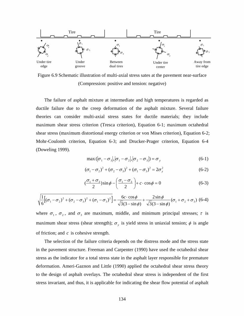
134
Under tire edge
1σ
3σ
1σ 1σ
1σ1σ
3σ
3σ3σ
3σ
Away from tire edge
Under tire center
Between dual tires
Under groove
TireTire
Figure 6.9 Schematic illustration of multi-axial stress sates at the pavement near-surface
(Compression: positive and tension: negative)
The failure of asphalt mixture at intermediate and high temperatures is regarded as
ductile failure due to the creep deformation of the asphalt mixture. Several failure
theories can consider multi-axial stress states for ductile materials; they include
maximum shear stress criterion (Tresca criterion), Equation 6-1; maximum octahedral
shear stress (maximum distortional energy criterion or von Mises criterion), Equation 6-2;
Mohr-Coulomb criterion, Equation 6-3; and Drucker-Prager criterion, Equation 6-4
(Doweling 1999).
max yσσσσσσσ =−−− ),,( 322131 (6-1)
2231
232
221 2)()()( yσσσσσσσ =−+−+− (6-2)
0cos2
sin)2
( 3131 =⋅+
−
−+ φσσφσσ c (6-3)
[ ] )()sin3(3
sin2)sin3(3
cos6)()()(61
3212
312
322
21 σσσφ
φφφσσσσσσ ++
−+
−⋅
=−+−+−c (6-4)
where 1σ , 2σ , and 3σ are maximum, middle, and minimum principal stresses; τ is
maximum shear stress (shear strength); yσ is yield stress in uniaxial tension; φ is angle
of friction; and c is cohesive strength.
The selection of the failure criteria depends on the distress mode and the stress state
in the pavement structure. Freeman and Carpenter (1990) have used the octahedral shear
stress as the indicator for a total stress state in the asphalt layer responsible for premature
deformation. Ameri-Gaznon and Little (1990) applied the octahedral shear stress theory
to the design of asphalt overlays. The octahedral shear stress is independent of the first
stress invariant, and thus, it is applicable for indicating the shear flow potential of asphalt
135
concrete without considering volumetric deformation. However, the octahedral shear
stress criterion shows no hydrostatic pressure dependence and failure is therefore a
function of only shear.
The Mohr-Coulomb failure criterion is widely used in soil mechanics. Asphalt
mixtures are composed of aggregate, asphalt, and air, and are analogous to soils
composed of soil solids, water, and air. At intermediate-to-high temperatures, the asphalt
concrete may be modeled as Mohr–Coulomb materials with both cohesive and granular
properties. However, the Mohr-Coulomb criterion ignores the effects of the intermediate
principal stress and represents an irregular hexagonal pyramid in the stress space. The
Drucker-Prager model is a smooth version of the Mohr–Coulomb model because it
modifies the Mohr-Coulomb yield function to avoid singularities associated with corners.
Both Mohr–Coulomb and Drucker–Prager criteria are pressure dependent models and
consider the compressive strength of the material is much greater than its tensile strength.
They have been used in this study to compare failure potential at the pavement near-
surface under various loading conditions. However, both models may not capture the
distinction between asphalt concrete damage behavior under compression and extension
(not necessarily tension) loading conditions (Masad et al. 2005). .
The parameters c andφ in Mohr–Coulomb and Drucker–Prager criteria are typically
obtained from triaxial strength tests conducted at various confinement levels. Generally,
c is equal to zero for pure granular material, while φ is equal to zero for pure cohesive
material. For asphalt mixtures, the parameters c andφ can be obtained from a
combination of unconfined tensile and compressive strength tests. A simple linear
relationship has been found between the cohesion parameter and the indirect tensile
strength of asphalt concrete (Gokhale et al. 2005).
The strength of asphalt concrete develops from both cohesion and the frictional
resistance. Cohesion is caused by the viscosity of asphalt binder and affected by the
binder grade and content; while the friction comes from the aggregate shape, texture, and
the interlock of aggregate skeleton. Previous research has shown that the friction angle of
asphalt concrete is relatively independent of test temperature and strain rate, whereas the
cohesion coefficient of asphalt concrete decreases as the test temperatures increases or
the strain rate decreases (Tan et al. 1994). In this study, for the purpose of evaluating the
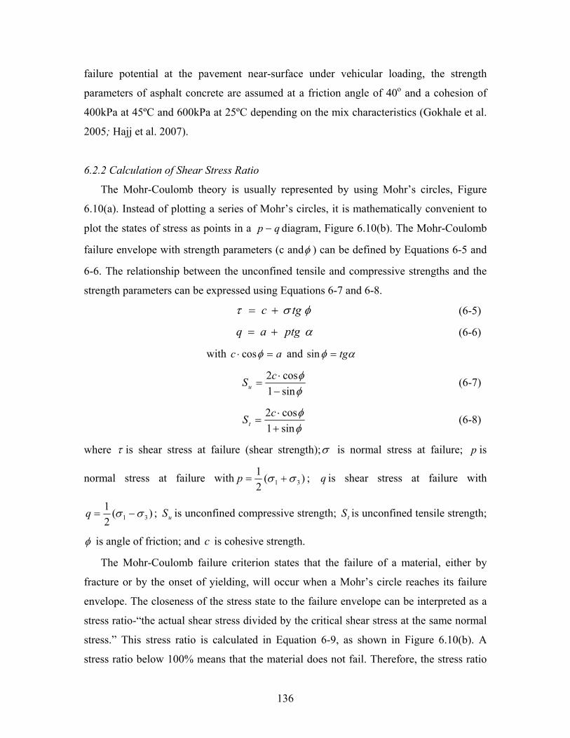
136
failure potential at the pavement near-surface under vehicular loading, the strength
parameters of asphalt concrete are assumed at a friction angle of 40o and a cohesion of
400kPa at 45ºC and 600kPa at 25ºC depending on the mix characteristics (Gokhale et al.
2005; Hajj et al. 2007).
6.2.2 Calculation of Shear Stress Ratio
The Mohr-Coulomb theory is usually represented by using Mohr’s circles, Figure
6.10(a). Instead of plotting a series of Mohr’s circles, it is mathematically convenient to
plot the states of stress as points in a qp − diagram, Figure 6.10(b). The Mohr-Coulomb
failure envelope with strength parameters (c andφ ) can be defined by Equations 6-5 and
6-6. The relationship between the unconfined tensile and compressive strengths and the
strength parameters can be expressed using Equations 6-7 and 6-8.
φστ tgc += (6-5)
αptgaq += (6-6)
with ac =⋅ φcos and αφ tg=sin
φφ
sin1cos2
−⋅
=cSu (6-7)
φφ
sin1cos2
+⋅
=cSt (6-8)
where τ is shear stress at failure (shear strength);σ is normal stress at failure; p is
normal stress at failure with )(21
31 σσ +=p ; q is shear stress at failure with
)(21
31 σσ −=q ; uS is unconfined compressive strength; tS is unconfined tensile strength;
φ is angle of friction; and c is cohesive strength.
The Mohr-Coulomb failure criterion states that the failure of a material, either by
fracture or by the onset of yielding, will occur when a Mohr’s circle reaches its failure
envelope. The closeness of the stress state to the failure envelope can be interpreted as a
stress ratio-“the actual shear stress divided by the critical shear stress at the same normal
stress.” This stress ratio is calculated in Equation 6-9, as shown in Figure 6.10(b). A
stress ratio below 100% means that the material does not fail. Therefore, the stress ratio
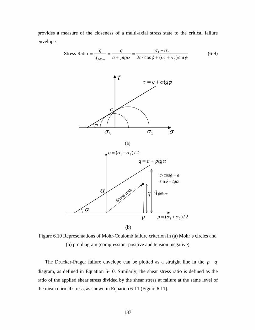
137
provides a measure of the closeness of a multi-axial stress state to the critical failure
envelope.
Stress Ratio φσσφ
σσα sin)(cos2 31
31
++⋅−
=+
==cptga
qfailure
(6-9)
τ
σ
c
ϕ1σ3σ
φστ tgc +=
(a)
a
α
failureqqStre
ss path
2/)( 31 σσ +=p
2/)( 31 σσ −=q
p
αptgaq +=
ac =⋅ φcosαφ tg=sin
(b)
Figure 6.10 Representations of Mohr-Coulomb failure criterion in (a) Mohr’s circles and
(b) p-q diagram (compression: positive and tension: negative)
The Drucker-Prager failure envelope can be plotted as a straight line in the qp −
diagram, as defined in Equation 6-10. Similarly, the shear stress ratio is defined as the
ratio of the applied shear stress divided by the shear stress at failure at the same level of
the mean normal stress, as shown in Equation 6-11 (Figure 6.11).

138
BApq += (6-10)
with ϕϕ
sin3sin6−
=A and ϕϕ
sin3cos6
−⋅
=cB
Stress Ratio ϕϕ
ϕcos6sin2
)sin3(3
1
2
cIJ
BApq
failure +−
=+
== (6-11)
where p is the mean normal stress at failure with )(31
31
3211 σσσ ++== Ip ; q is the
shear stress at failure with [ ]231
232
2212 )()()(
613 σσσσσσ −+−+−== Jq ; 1I is the
first stress invariant; 2J is the second invariant of deviatoric stress; φ is the angle of
friction; and c is the cohesive strength.
failureqq
p
Stress p
ath
23Jq =BApq +=
ϕϕ
sin3sin6−
=A
ϕϕ
sin3cos6−
=cB
131 Ip =
Figure 6.11 Representation of Drucker-Prager failure criterion in p-q diagram
(compression: positive and tension: negative)
6.2.3 Stress Invariants at Pavement Near-Surface
Figures 6.12 and 6.13 show the load-induced multi-axial stress states that occur at a
depth of 50mm under the pavement surface, respectively at 25ºC and 45ºC. The loading
is represented by the measured 3-D tire contact stresses under a dual-tire assembly
(35.5kN, 724kPa, and 8km/h). The figures show that similar stress distributions but
different stress magnitudes were found when using the Mohr–Coulomb and Drucker–
Prager criteria, respectively.
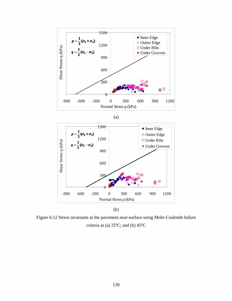
139
0
300
600
900
1200
1500
-900 -600 -300 0 300 600 900 1200Normal Stress p (kPa)
Shea
r Stre
ss q
(kPa
)
Inner EdgeOutter EdgeUnder RibsUnder Grooves
(a)
0
300
600
900
1200
1500
-900 -600 -300 0 300 600 900 1200Normal Stress p (kPa)
Shea
r Stre
ss q
(kPa
)
Inner EdgeOutter EdgeUnder RibsUnder Grooves
(b)
Figure 6.12 Stress invariants at the pavement near-surface using Mohr-Coulomb failure
criteria at (a) 25ºC; and (b) 45ºC
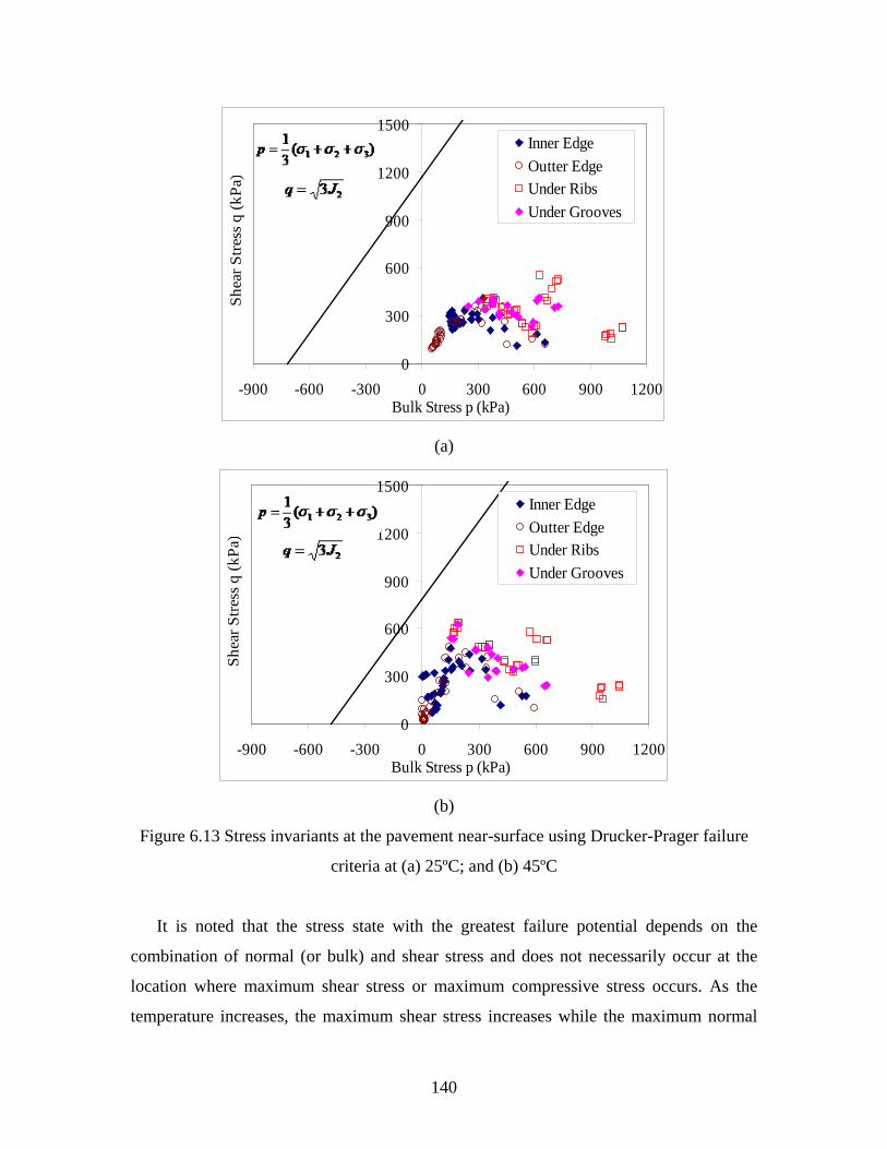
140
0
300
600
900
1200
1500
-900 -600 -300 0 300 600 900 1200Bulk Stress p (kPa)
Shea
r Stre
ss q
(kPa
)
Inner EdgeOutter EdgeUnder RibsUnder Grooves
(a)
0
300
600
900
1200
1500
-900 -600 -300 0 300 600 900 1200Bulk Stress p (kPa)
Shea
r Stre
ss q
(kPa
)
Inner EdgeOutter EdgeUnder RibsUnder Grooves
(b)
Figure 6.13 Stress invariants at the pavement near-surface using Drucker-Prager failure
criteria at (a) 25ºC; and (b) 45ºC
It is noted that the stress state with the greatest failure potential depends on the
combination of normal (or bulk) and shear stress and does not necessarily occur at the
location where maximum shear stress or maximum compressive stress occurs. As the
temperature increases, the maximum shear stress increases while the maximum normal
141
(or bulk) stress keeps relatively constant. This indicates that the shear effect becomes
more significant at high temperatures. At some locations, the shear stresses are greater
than the normal stresses, which results in producing critical stress states close to the
failure envelope. Interestingly, no negative normal stress state was found at the pavement
near-surface. This indicates that the failure at the pavement near-surface is more like
shear failure instead of tensile failure for thick asphalt pavements.
As expected, the vehicle load would not cause pavement failure due to one-pass
loading because of the relatively lower stress compared to the failure envelope. After
repetitive loading, the damage can accumulate because the material stiffness is reduced
and the stress may reach the failure envelope. Instead of implementing a full plastic and
damage model, the stress ratio under one-pass loading is used in this study to evaluate the
failure potential at the pavement near-surface.
6.2.4 Near-Surface Pavement Shear Failure Potential
The critical failure locations in the asphalt layer can be determined by plotting
contours of the calculated shear stress ratios. Figures 6.14(a) and (b) plot the calculated
stress ratios within the asphalt layer under the loading of a dual-tire assembly at 25ºC
(35.5kN, 724kPa, and 8km/h), respectively, using the Mohr–Coulomb and Drucker–
Prager criteria. Due to the symmetry of dual tires, only the asphalt layer under one tire of
the dual-tire assembly was plotted. The stress ratio contours have the similar trends when
using the two failure criteria.
The stress ratio has a local concentration at the pavement surface due to the localized
tire contact stresses (non-uniform vertical and tangential stresses) under each tire rib. The
stress states at tire edges or under the grooves between adjacent ribs where the
confinement is lower are more critical than the stress states under tire ribs. In this case,
the stress state at the bottom of the asphalt layer is more critical. The critical stress state
at the bottom of the asphalt layer is caused by high tensile stresses due to bending, while
the critical stress state at the pavement near-surface is mainly caused by high shear
stresses at low confinements. However, the surface-initiated cracking potential may
increase after considering the effect of thermal stress, construction defects (segregation or
joints between pavers), or binder brittleness due to aging.
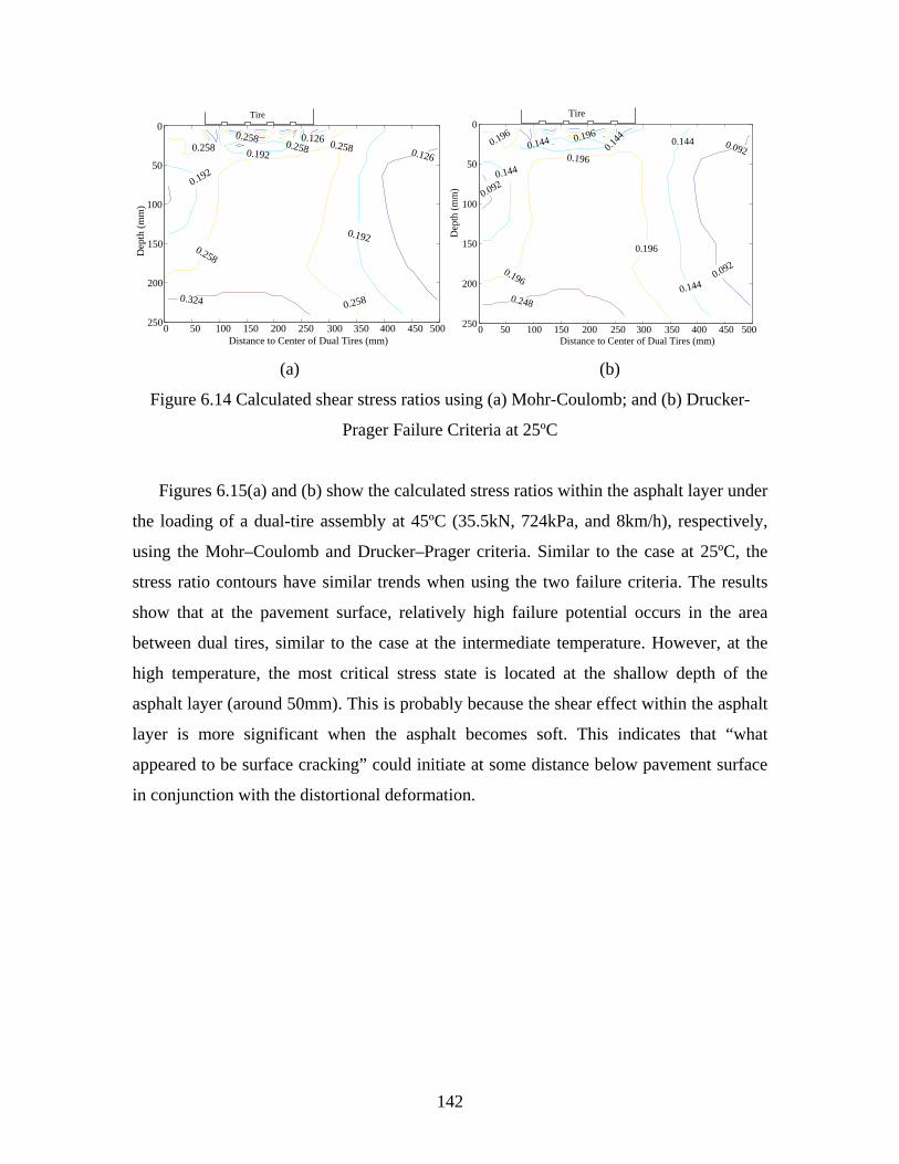
142
0.1260.126
0.192
0.192
0.192
0.258
0.258
0.258
0.2580.258
0.258
0.324
Distance to Center of Dual Tires (mm)
Dep
th (m
m)
0 50 100 150 200 250 300 350 400 450 500
0
50
100
150
200
250
Tire
0.092
0.092
0.092
0.144
0.1440.144
0.144
0.196
0.196
0.196
0.1960.196
0.248
0 50 100 150 200 250 300 350 400 450 500
0
50
100
150
200
250
0.144
Tire
Distance to Center of Dual Tires (mm)
Dep
th (m
m)
(a) (b)
Figure 6.14 Calculated shear stress ratios using (a) Mohr-Coulomb; and (b) Drucker-
Prager Failure Criteria at 25ºC
Figures 6.15(a) and (b) show the calculated stress ratios within the asphalt layer under
the loading of a dual-tire assembly at 45ºC (35.5kN, 724kPa, and 8km/h), respectively,
using the Mohr–Coulomb and Drucker–Prager criteria. Similar to the case at 25ºC, the
stress ratio contours have similar trends when using the two failure criteria. The results
show that at the pavement surface, relatively high failure potential occurs in the area
between dual tires, similar to the case at the intermediate temperature. However, at the
high temperature, the most critical stress state is located at the shallow depth of the
asphalt layer (around 50mm). This is probably because the shear effect within the asphalt
layer is more significant when the asphalt becomes soft. This indicates that “what
appeared to be surface cracking” could initiate at some distance below pavement surface
in conjunction with the distortional deformation.
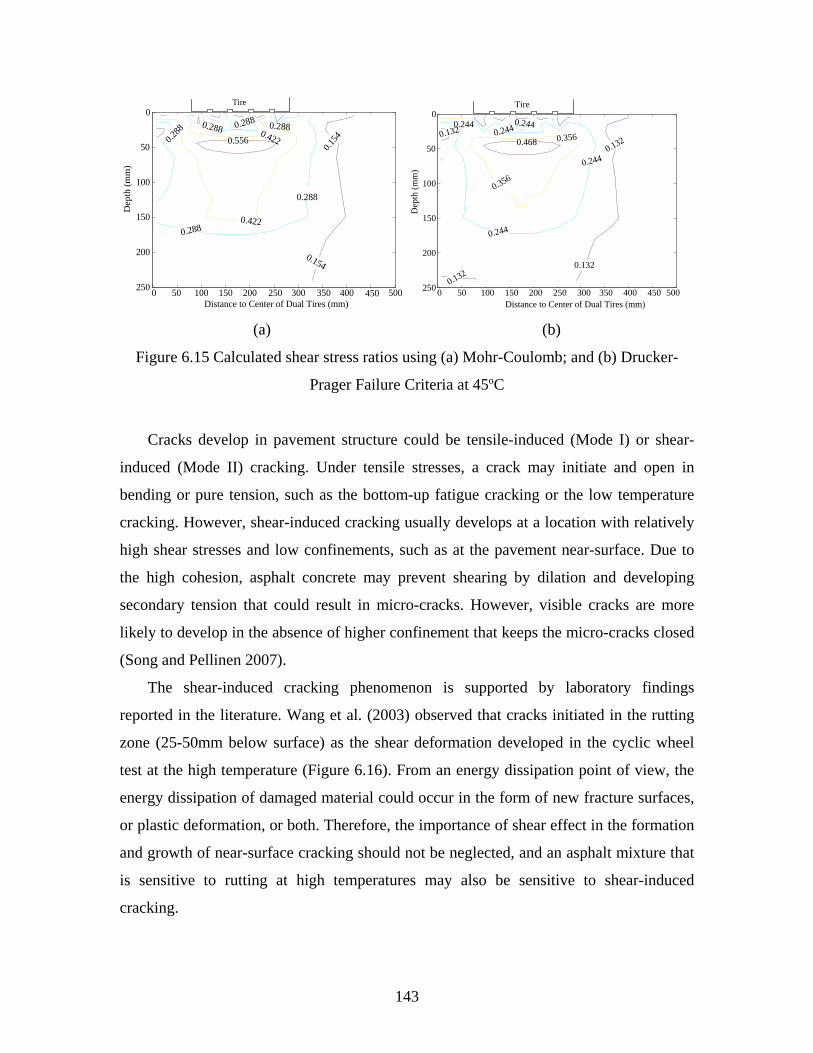
143
0.154
0.154
0.288
0.288
0.2880.2880.2
880.288
0.422
0.422
0.556
0 50 100 150 200 250 300 350 400 450 500
0
50
100
150
200
250
Tire
Distance to Center of Dual Tires (mm)
Dep
th (m
m)
0.132
0.132
0.132
0.132 0.244
0.244
0.244
0.244 0.244
0.356
0.3560.468
0 50 100 150 200 250 300 350 400 450 500
0
50
100
150
200
250
Tire
Distance to Center of Dual Tires (mm)
Dep
th (m
m)
(a) (b)
Figure 6.15 Calculated shear stress ratios using (a) Mohr-Coulomb; and (b) Drucker-
Prager Failure Criteria at 45ºC
Cracks develop in pavement structure could be tensile-induced (Mode I) or shear-
induced (Mode II) cracking. Under tensile stresses, a crack may initiate and open in
bending or pure tension, such as the bottom-up fatigue cracking or the low temperature
cracking. However, shear-induced cracking usually develops at a location with relatively
high shear stresses and low confinements, such as at the pavement near-surface. Due to
the high cohesion, asphalt concrete may prevent shearing by dilation and developing
secondary tension that could result in micro-cracks. However, visible cracks are more
likely to develop in the absence of higher confinement that keeps the micro-cracks closed
(Song and Pellinen 2007).
The shear-induced cracking phenomenon is supported by laboratory findings
reported in the literature. Wang et al. (2003) observed that cracks initiated in the rutting
zone (25-50mm below surface) as the shear deformation developed in the cyclic wheel
test at the high temperature (Figure 6.16). From an energy dissipation point of view, the
energy dissipation of damaged material could occur in the form of new fracture surfaces,
or plastic deformation, or both. Therefore, the importance of shear effect in the formation
and growth of near-surface cracking should not be neglected, and an asphalt mixture that
is sensitive to rutting at high temperatures may also be sensitive to shear-induced
cracking.
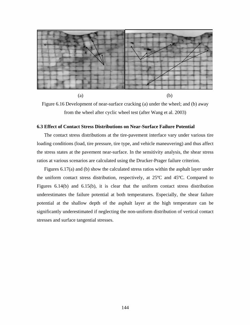
144
(a) (b)
Figure 6.16 Development of near-surface cracking (a) under the wheel; and (b) away
from the wheel after cyclic wheel test (after Wang et al. 2003)
6.3 Effect of Contact Stress Distributions on Near-Surface Failure Potential
The contact stress distributions at the tire-pavement interface vary under various tire
loading conditions (load, tire pressure, tire type, and vehicle maneuvering) and thus affect
the stress states at the pavement near-surface. In the sensitivity analysis, the shear stress
ratios at various scenarios are calculated using the Drucker-Prager failure criterion.
Figures 6.17(a) and (b) show the calculated stress ratios within the asphalt layer under
the uniform contact stress distribution, respectively, at 25ºC and 45ºC. Compared to
Figures 6.14(b) and 6.15(b), it is clear that the uniform contact stress distribution
underestimates the failure potential at both temperatures. Especially, the shear failure
potential at the shallow depth of the asphalt layer at the high temperature can be
significantly underestimated if neglecting the non-uniform distribution of vertical contact
stresses and surface tangential stresses.
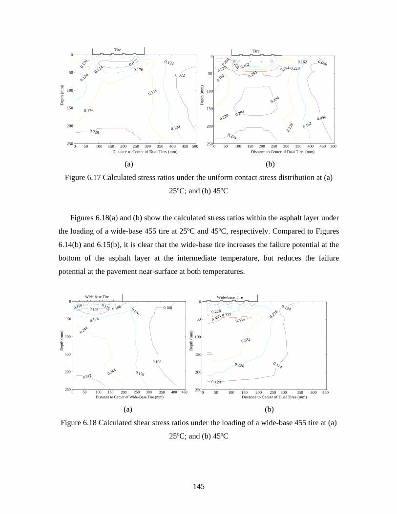
145
0.072
0.072
0.124
0.124
0.124
0.124
0.176
0.176
0.176
0.176
0.228
0 50 100 150 200 250 300 350 400 450 500
0
50
100
150
200
250
Tire
Distance to Center of Dual Tires (mm)
Dep
th (m
m)
0.096
0.096
0.162
0.1620.162
0.162
0.228
0.228
0.228
0.228
0.228
0.294
0.294
0.2940.294
0.294
0.294
0 50 100 150 200 250 300 350 400 450 500
0
50
100
150
200
250
Tire
Distance to Center of Dual Tires (mm)
Dep
th (m
m)
(a) (b)
Figure 6.17 Calculated stress ratios under the uniform contact stress distribution at (a)
25ºC; and (b) 45ºC
Figures 6.18(a) and (b) show the calculated stress ratios within the asphalt layer under
the loading of a wide-base 455 tire at 25ºC and 45ºC, respectively. Compared to Figures
6.14(b) and 6.15(b), it is clear that the wide-base tire increases the failure potential at the
bottom of the asphalt layer at the intermediate temperature, but reduces the failure
potential at the pavement near-surface at both temperatures.
0.108
0.1080.1080.108
0.176
0.176
0.176
0.1760.176
0.244
0.244
0.312
0 50 100 150 200 250 300 350 400 450
0
50
100
150
200
250
Distance to Center of Wide-Base Tire (mm)
Dep
th (m
m)
Wide-base Tire
0.124
0.124
0.124
0.228
0.2280.228
0.332
0.3320.436
0.436
0 50 100 150 200 250 300 350 400 450
0
50
100
150
200
250
Distance to Center of Dual Tires (mm)
Dep
th (m
m)
Wide-base Tire
(a) (b)
Figure 6.18 Calculated shear stress ratios under the loading of a wide-base 455 tire at (a)
25ºC; and (b) 45ºC
146
Figures 6.19 and 6.20 show the calculated stress ratios within the asphalt layer under
heavy load (53.6kN) and high tire inflation pressure (966kPa), respectively, at 25ºC and
45ºC. At the intermediate temperature, the surface failure potential at the inner tire edge
becomes more critical as the load increases, while the increase of surface failure potential
is relatively not significant as the tire pressure increases (compared to Figures 6.14(b)).
At the high temperature, the heavy load mainly increases the area of stress concentration
with a slightly increased peak stress ratio; while the high tire pressure significantly
increases the peak stress ratio in a small area of stress concentration (compared to Figure
6.15(b)). Again, these observations are related to the variations of the localized contact
stress distributions as the load or tire pressure increases.
0.106
0.106
0.106
0.182
0.1820.1820.182
0.182
0.258
0.258
0.258
0.334
0 50 100 150 200 250 300 350 400 450 500
0
50
100
150
200
250
Tire
Distance to Center of Dual Tires (mm)
Dep
th (m
m)
0.144
0.144
0.268
0.268
0.268 0.392
0.3920.392
0.392
0.516
0.516
0 50 100 150 200 250 300 350 400 450 500
0
50
100
150
200
250
Tire
Distance to Center of Dual Tires (mm)
Dep
th (m
m)
(a) (b)
Figure 6.19 Calculated shear stress ratios under heavy load at (a) 25ºC; and (b) 45ºC
0.102
0.102
0.102
0.154
0.1540.1540.154
0.154
0.154
0.206
0.206
0.206
0.206 0.206
0.258
0 50 100 150 200 250 300 350 400 450 500
0
50
100
150
200
250
Tire
Distance to Center of Dual Tires (mm)
Dep
th (m
m)
0.172
0.172
0.172
0.172
0.334
0.334
0.3340.496 0.496
0.658
0 50 100 150 200 250 300 350 400 450 500
0
50
100
150
200
250
Tire
Distance to Center of Dual Tires (mm)
Dep
th (m
m)
(a) (b)
Figure 6.20 Calculated shear stress ratios at high tire pressure at (a) 25ºC; and (b) 45ºC
147
Figures 6.21 and 6.22 show the calculated stress ratios within the asphalt layer under
vehicle maneuvering at 25ºC and 45ºC, respectively. The tire-pavement contact stresses
were obtained from the tire-pavement interaction model using a surface friction
coefficient of 0.8 at tire braking and slip angle of 5º at tire cornering. Compared to
Figures 6.14(b) and 6.15(b), the results show that tire braking or cornering causes the
greater failure potential, especially at the high temperature. It is noted that as the tire is
cornering, the critical stress states are concentrated towards one side of the tire because
tire cornering causes high vertical and transverse contact stresses shifted to one side of
the tire contact area. 0.1
12
0.112
0.112
0.164
0.1640.1640.164
0.164
0.216
0.216
0.216
0.216
0.268
0 50 100 150 200 250 300 350 400 450 500
0
50
100
150
200
250
0.2160.216
Tire
Distance to Center of Dual Tires (mm)
Dep
th (m
m)
0.166
0.166
0.166
0.166
0.312
0.312
0.4580.458
0.458
0.4580.604
0 50 100 150 200 250 300 350 400 450 500
0
50
100
150
200
250
Tire
Distance to Center of Dual Tires (mm)
Dep
th (m
m)
(a) (b)
Figure 6.21 Calculated shear stress ratios due to tire braking at (a) 25ºC; and (b) 45ºC
0.098
0.098
0.156
0.156
0.1560.156
0.15
6
0.214
0.214
0.214
0.214
0.21
4
0.272
0 50 100 150 200 250 300 350 400 450 500
0
50
100
150
200
250
Tire
Distance to Center of Dual Tires (mm)
Dep
th (m
m)
0.148
0.148
0.286
0.286
0.2860.424
0.4240.424
0.562
0 50 100 150 200 250 300 350 400 450 500
0
50
100
150
200
250
Tire
Distance to Center of Dual Tires (mm)
Dep
th (m
m)
(a) (b)
Figure 6.22 Calculated shear stress ratios due to tire cornering at (a) 25ºC; and (b) 45ºC
148
Table 6.4 summarizes the shear stress ratios at the pavement near-surface at critical
loading conditions with respect to the normal loading condition (35.5kN, 724kPa, and
8km/h). The results clearly show that high tire pressure is detrimental to the shear failure
at the shallow depth of the asphalt layer at high temperatures, while overload can
significantly increase the surface failure potential at intermediate temperatures.
Table 6.4 Stress Ratios Caused by Critical Loading Conditions
Case Load
(kN)
Pressure
(kPa)
Vehicle
Maneuvering
Stress ratio at
surface at 25°C
Stress ratio at shallow
depth at 45°C
1 35.5 724 No 0.196 0.468
2 35.5 966 No 0.206 0.658
3 53.6 724 No 0.258 0.516
4 35.5 724 Braking 0.216 0.604
5 35.5 724 Cornering 0.214 0.562
6.4 Effect of Structure Characteristics on Near-Surface Failure Potential
Since the failure potential at the pavement near-surface is related to other factors in
addition to loading, the effects of pavement structure characteristics on the stress states at
the pavement near-surface were investigated, such as the asphalt layer stiffness gradient,
interface bonding condition, and underlying support.
For thick asphalt pavements, the stiffness gradient in the asphalt layer could be
caused by variations in the characteristics of each course, aging of surface layer, and
temperature gradients. Changes in temperature during the day and night would produce
high stiffness variations in the asphalt layer. In this study, a temperature profile is
assumed by introducing a rate of linear temperature differential of 1.1ºC/cm within the
asphalt layer based on a previous study (Myers et al. 1998). For the purpose of
comparison with the case of the uniform temperature of 25ºC, the average temperature is
kept at 25ºC at the middle of the asphalt layer for both negative and positive temperature
gradients (Figure 6.23). The stiffness variation due to the negative temperature gradient is
similar to the case that the stiffness of the asphalt layer decreases as the depth increases.
149
Figures 6.24(a) and (b) show the calculated stress ratios within the asphalt layer under
the loading of a dual-tire assembly for the negative and positive temperature gradients,
respectively. It was found that the critical stress states are located at 75-150mm below the
pavement surface when the asphalt layer has the negative temperature gradient. For the
negative temperature gradient, the calculated critical stress ratios are greater than those
obtained from the uniform temperature case, as shown in Figure 6.14(b). On the other
hand, the critical stress states are located at the bottom of the asphalt layer when the
asphalt layer has the positive temperature gradient.
11oC
39oC
Dense-graded surface(50 mm)
Polymer-modified binder layer(115 mm)
Standard binder layer(89 mm)
25oC
11oC
39oC
25oC
(a) (b)
Figure 6.23 Illustration of (a) negative and (b) positive temperature gradients in
the asphalt layer
0.102
0.102
0.102
0.102
0.164
0.164
0.164
0.164
0.1640.164
0.164
0.2260.226
0.226
0.226
0.226
0.288
0.288
0.288
0 50 100 150 200 250 300 350 400 450 500
0
50
100
150
200
250
Tire
Distance to Center of Dual Tires (mm)
Dep
th (m
m)
0.168
0.1680.168
0.168
0.168
0.168
0.168
0.168 0.168
0.2860.286
0.4040.522
0 50 100 150 200 250 300 350 400 450 500
0
50
100
150
200
250
Tire
Distance to Center of Dual Tires (mm)
Dep
th (m
m)
(a) (b)
Figure 6.24 Calculated shear stress ratios for the (a) negative; and (b) positive
temperature gradients
150
The general assumption in the design of thick asphalt pavements is that the asphalt
layers are fully bonded together without relative slip. Debonding describes a condition
where adjacent asphalt layers lose adhesion to one another. In the analysis, the debonding
between asphalt layers is modeled as two separate layers with frictional interface, and the
coefficient of friction is assumed equal to one.
The calculated stress ratios within the asphalt layers under the loading of a dual-tire
assembly at 25ºC were plotted in Figures 6.25(a) and (b), respectively, for the first and
second interface debonding. The first interface is between the dense-graded surface layer
(50mm) and the polymer-modified binder layer (115mm), while the second interface is
between the polymer-modified binder layer and the standard binder layer (89mm).
Compared to Figure 6.14(b), the debonding significantly increases the critical stress ratio
around the debonded interface, especially for the debonded first interface. This indicates
that debonding under the wearing surface could cause near-surface cracking to initiate at
the bottom of the surface layer and propagate upward. This is in agreement with the field
observation reported by Willis and Timm (2007) (Figure 6.26). Hence, the achievement
of adequate bonding between asphalt layers during construction should be emphasized
for thick asphalt pavements.
0.163
0.163
0.163
0.163
0.163
0.311
0.311
0.311 0.4620.612
0 50 100 150 200 250 300 350 400 450 500
0
50
100
150
200
250
Tire
Distance to Center of Dual Tires (mm)
Dep
th (m
m)
0.112
0.1120.112
0.112
0.1120.112
0.112
0.2140.214
0.214
0.214
0.214
0.316
0.3160.418
0 50 100 150 200 250 300 350 400 450 500
0
50
100
150
200
250
Tire
Distance to Center of Dual Tires (mm)
Dep
th (m
m)
(a) (b)
Figure 6.25 Calculated shear stress ratios with debonding at the (a) first; and (b) second
interface
151
Figure 6.26 Development of near-surface cracking due to debonding (after Wills and
Timm 2003)
Figures 6.27(a) and (b) show the calculated stress ratios within the asphalt layer under
the loading of a dual-tire assembly at 25ºC with a weak (150MPa) and strong (700MPa)
subgrade support, respectively. The results show that the failure potential in the asphalt
layer decreases as the subgrade support becomes stronger, especially for the failure
potential at the bottom of the asphalt layer. It is noted that as the subgrade support
becomes stronger, the critical failure location could shift to the upper asphalt layer close
to the pavement surface. This indicates that the failure potential at the pavement near-
surface could increase as the underlying layer is very stiff.
0.1210.121
0.121
0.121
0.213
0.213
0.213
0.213
0.213
0.304
0.304
0.391
0 50 100 150 200 250 300 350 400 450 500
0
50
100
150
200
250
Tire
Distance to Center of Dual Tires (mm)
Dep
th (m
m)
0.078
0.0780.126
0.126
0.126
0.174
0.174
0.174
0.174 0.1740.174
0.222
0.2220.222
0 50 100 150 200 250 300 350 400 450 500
0
50
100
150
200
250
Tire
Distance to Center of Dual Tires (mm)
Dep
th (m
m)
(a) (b)
Figure 6.27 Calculated shear stress ratios with a (a) weak and (b) strong subgrade support
152
6.5 Summary
In this chapter, strain responses responsible for near-surface failure in thick asphalt
pavements were investigated at various loading scenarios. The analysis results indicate
that surface-initiated cracking cannot be induced by tension only and the effect of shear is
important and can not be neglected. In order to evaluate the failure potential at multi-
axial stress states, a shear stress ratio concept based on the Drucker-Prager failure
criterion was proposed.
It was found that cracks may initiate at the pavement surface at intermediate
temperatures. However, at high temperatures, shear-induced cracking becomes more
critical and may initiate at the shallow depth below the pavement surface in conjunction
with distortional deformation. The failure potential at the pavement near-surface is
affected by tire-pavement contact stress distributions, which is dependent on load, tire
inflation pressure, tire configuration, and vehicle maneuvering. In addition, the analysis
results show that the critical failure location in the thick asphalt layer vary as the
pavement structure characteristics (stiffness gradient, interface bonding, or underlying
support) change.
153
CHAPTER 7 FINDINGS, CONCLUSIONS, AND RECOMMENDATIONS
In this dissertation, the mechanism of tire-pavement interaction and the effect of tire-
pavement interaction on pavement responses were analyzed through a decoupled
modeling approach. First, an air-inflated 3-D tire model was built and the interaction
between a tire and a non-deformable pavement surface was simulated. The tire is
modeled as a composite structure including rubber and reinforcement. The steady-state
tire rolling process was simulated using an Arbitrary Lagrangian Eulerian (ALE)
formulation. The developed tire-pavement interaction model is used to evaluate the
mechanism of load distribution at the tire-pavement interface under various tire loading
and rolling conditions. Second, a 3-D FE model of flexible pavement was developed to
analyze pavement responses under various loading scenarios. This model utilizes implicit
dynamic analysis and simulates vehicular loading as a continuous moving load with
three-dimensional contact stresses at the tire-pavement interface. In the pavement model,
the asphalt layer is modeled as a linear viscoelastic material and the granular base layer is
modeled as a nonlinear anisotropic material. The FE model is used to analyze critical
pavement responses in thin and thick asphalt pavements considering different damage
mechanisms.
7.1 Findings
The following findings were obtained from the analyses:
Tire-Pavement Interaction
1) Both the prediction and measurements show that the vertical contact stresses and
localized tangential contact stresses are non-uniformly distributed at the tire-
pavement interface. At the static loading condition, both the vertical and
transverse contact stresses have a convex shape along the contact length; while
the longitudinal contact stresses have a reversed distribution pattern. It is noted
that the transverse contact stress increases in magnitude with the lateral distance
from the center of each rib and reaches its maximum at the edge of each rib.
2) The load and tire inflation pressure affect the tire-pavement contact stress
distributions in different ways. As the load increases, the vertical contact stresses
154
at tire edges and the longitudinal contact stresses increase. On the other hand, as
the tire inflation pressure increases, the vertical contact stresses at tire center and
the transverse contact stresses increase. Therefore, at heavy load, the maximum
vertical contact stress may be located at tire edges; while at high tire inflation
pressure, the non-uniformity of vertical contact stress is the highest. The stress
ratio of the maximum contact stresses in three directions ranges from 1:0.23:0.07
to 1:0.31:0.30 as the load varies between 18 and 40kN and the tire inflation
pressure varies between 414 and 966kPa.
3) Vehicle maneuvering behavior significantly affects the magnitudes and
distributions of tire-pavement contact stresses. Compared to the free rolling
condition, tire braking/acceleration causes reduction in transverse contact stresses;
but significant increase in longitudinal contact stresses. The longitudinal contact
stresses at tire braking increase with the slip ratio until the tire reaches full
braking. As the tire is cornering, both the vertical and transverse contact stresses
are greater than those at the free rolling condition. The peak contact stresses at
tire cornering shift toward one side of the contact patch and increase as the slip
angle increases.
4) As the friction at the tire-pavement surface increases, the tangential tire-
pavement contact stresses at various rolling conditions and the vertical contact
stresses at tire cornering increase. It is reasonable to use the constant static
friction coefficient when predicting the tire-pavement contact stresses at the free
rolling condition or at the cornering condition with small slip angles. However,
using the constant friction model may overestimate the peak longitudinal contact
stress when the tire is sliding at the full braking condition.
1) Accurate pavement responses can only be predicted when the viscoelastic nature
of the asphalt layer and the nonlinear anisotropic behavior of the granular base
layer are integrated into the mechanistic model. The modulus distribution in the
base layer is not only affected by the wheel load, but also affected by the
Critical Pavement Responses and Failure Mechanism
155
temperature and vehicle speed due to the viscoelastic nature of the asphalt surface
layer.
2) It was found that neglecting the cross-anisotropic stress-dependent behavior of the
granular base layer could significantly underestimate fatigue cracking and rutting
potential in thin asphalt pavements; especially at high temperatures. However, the
stress-softening behavior of subgrade mainly affects the responses in the base
layer and subgrade.
3) The multi-axial stress state needs to be considered when evaluating near-surface
failure potential in thick asphalt pavements. The analysis results indicate that
surface-initiated cracking cannot be induced by tension only and the effect of
shear cannot be neglected. The calculated shear stress ratio based on the Drucker-
Prager failure criterion provides a reasonable indication for the failure at the
pavement near-surface at intermediate and high temperatures.
4) It was found that cracks may initiate at the pavement surface at intermediate
temperatures. At high temperatures, shear-induced cracking becomes more critical
and it may initiate at the shallow depth below the pavement surface in conjunction
with the distortional deformation. The critical failure location in thick asphalt
pavements is also affected by pavement structure characteristics, such as the
stiffness gradient, interface debonding, or underlying support.
1) Flexible pavement responses are sensitive to the loading input represented by the
tire-pavement contact stress distributions, especially when the asphalt layer is soft.
The analysis results show that compared to the uniform contact stress assumption,
the 3-D tire contact stresses cause greater fatigue cracking and primary rutting
potential but less failure potential in the base layer and subgrade in thin asphalt
pavements. In addition, assuming uniform contact stress distribution at the tire-
pavement interface underestimates near-surface failure potential in thick asphalt
pavements.
Effect of Tire-Pavement Interaction on Pavement Responses
2) For thin asphalt pavements, the heavy load mainly causes the increase of
responses in the subgrade, while the effect of tire inflation pressure is more
156
significant for the responses in the asphalt layer. In addition, the load effect is
more significant at intermediate temperatures; while the inflated tire pressure
effect is more significant at high temperatures. This indicates that the high shear-
resistant mixture is desired when the truck tire pressure is high in regions with
warm climates, while the axle weight limit should be enforced during spring
seasons on low-volume roads in order to minimize pavement damage.
3) The effects of load or inflated tire pressure on near-surface failure potential in
thick asphalt pavements are dependent on the variations of localized tire contact
stress distributions. At intermediate temperatures, surface failure potential at the
inner tire edges becomes more critical as the load increases, while the effect of
tire pressure is relatively not significant. However, at high temperatures, high tire
pressure significantly increases shear failure potential at the shallow depth of the
asphalt layer.
4) Tire braking and cornering induce high tangential contact stresses at the pavement
surface, which increase near-surface failure potential in thick asphalt pavements.
For thin asphalt pavements, tire cornering mainly increase rutting potential, while
tire braking mainly increase shoving/corrugation potential in the asphalt layer.
This indicates that the effect of vehicle maneuvering behavior should be
considered for pavement design at specific sites, such as intersections, pavement
sections with great slopes, or curved road sections.
5) The impact of wide-base tire on pavement damage depends on the predominant
failure mechanisms of the roadway. Compared to the conventional dual-tire
assembly, the new generation of wide-base tire results in similar or less primary
rutting potential in thin asphalt pavements and near-surface failure potential in
thick asphalt pavements, although it increases the damage potential at deeper
pavement depths, which is less pronounced in causing failure.
7.2 Conclusions
This study concludes that knowledge of tire-pavement contact stress distributions is
critical for pavement response prediction. Most importantly, the non-uniform distribution
of vertical contact stresses and the localized tangential contact stresses should be
157
considered in the mechanistic-empirical pavement design. The contact stress distributions
at the tire-pavement interface are affected by vehicle loading (wheel load and tire
inflation pressure), tire configuration (dual-tire assembly and wide-base tire), vehicle
maneuvering (braking/acceleration and cornering), and pavement surface friction.
Therefore, pavement damage should be quantified using accurate loading inputs that are
represented by realistic tire-pavement contact stress distributions.
Thin and thick asphalt pavements fail in different ways. Multiple distress modes
could happen in thin asphalt pavements, including bottom-up fatigue cracking and rutting
in each pavement layer. It was found that the interaction between the viscoelastic asphalt
layer and the nonlinear anisotropic granular base material plays an important role for the
stress distribution within a thin asphalt pavement structure under vehicular loading. In
thick asphalt pavements, near-surface cracking is a critical failure mechanism, which is
affected by the localized stress states and pavement structure characteristics. Particularly,
the effect of shear stress on the formation of near-surface cracking at multi-axial stress
states is important and can not be neglected, especially at high temperatures.
7.3 Recommendations for Future Study
Despite utilizing the advanced finite element model for the analysis of tire-pavement
interaction and pavement responses in this study, in order to better design long-lasting
pavements, the following tasks are recommended in future studies:
1) This study considers pavement surface as a rigid flat surface for the prediction of
tire-pavement contact stresses. Deformable road surfaces should be considered in
future studies to simulate the coupled tire-pavement interaction behavior. The
irregularities (texture) of pavement surfaces should also be considered. This
would be especially important when detailed tire-pavement interaction conditions
are studied; including rolling resistance, tire wear, and noise. This will allow
considering pavement durability, safety, and quietness.
2) Only one specific tire with one type of tread pattern was simulated in this study. It
is expected that the 3-D tire contact stress distributions depend on the tire
geometry, structure, and tread configuration. It is recommended that various tire
types including wide-base tires with different tread patterns should be modeled in
158
future studies and a large database of contact stresses should be created. This
database can be used not only for design of new pavements and overlays, but also
for setting reasonable axle load or pressure regulations for trucking operation. On
the other hand, this database would be beneficial for tire manufacturers to design
“pavement-friendly” tires.
3) Although the finite element method can consider many important aspects in
pavement modeling, it requires significant computation time and resource. For
pavement design purpose, a convenient and reliable method is desired to consider
the effects of tire-pavement interaction on pavement responses and damage
prediction. Therefore, a large database of pavement responses should be built
considering various loading conditions, environmental conditions, and pavement
structure characteristics. This database can be used to develop design monographs
or Artificial Neuro Network (ANN) for pavement design purpose.
4) Many studies have been conducted to characterize the fatigue behavior of asphalt
mixtures under the pure tension or bending stress states. The analysis results
presented in this dissertation clearly show that the shear effect can not be
neglected in the formation of near-surface cracking. Therefore, a laboratory
testing method that better simulates the material failure at multi-axial stress states
need to be developed and verified. Furthermore, a performance prediction model
should be developed for considering near-surface cracking mechanism in the
mechanistic-empirical pavement design. This model could be based on continuum
damage theory or fracture mechanics method and the effect of binder aging and
healing should be considered.
159
REFERENCES AASHTO (1999) Standard Method of Test for Determining the Resilient Modulus of
Soils and Aggregate Materials, AASHTO T307, Washington, D.C.
AASHTO (2003) Standard Method of Test for Determining the Creep Compliance and
Strength of Hot-Mix Asphalt (HMA) Using the Indirect Tensile Test Device,
AASHTO T322, Washington, D.C.
ABAQUS (2007) ABAQUS Analysis User’s Manual, Version 6.7, Habbit, Karlsson &
Sorenson, Inc, Pawtucket, RI.
Adu-Osei, A., Little, D.N. and Lytton, R.L. (2001) “Cross-anisotropic Characterization of
Unbound Granular Materials,” Transportation Research Record, No.1757, TRB,
Washington, D.C., pp. 82-91.
Al-Qadi, I.L., Loulizi, A., Janajreh, I., and Freeman, T.E. (2002) “Pavement Response to
Dual Tires and New Wide-Base Tires at Same Tire Pressure,” Transportation
Research Record, No. 1806, TRB, Washington, D.C., pp. 38-47.
Al-Qadi, I.L., Elseifi, M.A. and Yoo, P.J. (2005) “Characterization of Pavement Damage
Due to Different Tire Configurations,” Journal of the Association of Asphalt Paving
Technologists, Vol. 84, AAPT, pp. 921-962.
Al-Qadi, I.L., and Elseifi, M.A. (2007) “State-of-the-Practice of the New Generation of
Wide-Base Tire and Its Impact on Trucking Operations,” Transportation Research
Record, No. 2008, TRB, Washington, D.C., pp. 100-109.
Al-Qadi, I.L., Tutumluer, E., Dessouky, S.H., Kwon, J. (2007) Effectiveness of Geogrid-
Reinforcement in Flexible Pavements: A Full-Scale Testing, Final Report to Tensar
Earth Technologies, Inc., University of Illinois, Urbana-Champaign, IL.
Al-Qadi, I.L. and Yoo, P.J. (2007) “Effect of Surface Tangential Contact Stress on
Flexible Pavement Response,” Journal of the Association of Asphalt Pavement
Technologist, Vol. 76, AAPT, pp. 663-692.
160
Al-Qadi, I.L., Wang, H., Yoo, P.J., and Dessouky, S.H. (2008) “Dynamic Analysis and
In-Situ Validation of Perpetual Pavement Response to Vehicular Loading,”
Transportation Research Record, No. 2087, TRB, Washington, D.C., pp. 29-39.
Al-Qadi, I.L., and Wang, H. (2009) “Full-depth Pavement Responses under Various Tire
Configurations: Accelerated Pavement Testing and Finite Element Modeling,”
Journal of the Association of Asphalt Paving Technologists, Vol. 78, AAPT, pp. 645-
680.
Ameri-Gaznon, M., and Little, D.N. (1990) “Octahedral Shear Stress Analyses of an ACP
Overlay on a Rigid Base,” Journal of the Association of Asphalt Paving Technologists,
Vol. 59, AAPT, pp. 443-476.
ARA, Inc., ERES Division, (2004) Guide for Mechanistic-Empirical Design of New and
Rehabilitated Pavement Structures, NCHRP 1-37A Final Report, TRB, Washington,
D.C.
Asphalt Institute, (1982) Research and Development of the Asphalt Institute’s Thickness
Design Manual (MS-1), Research Report 82-1, 9th ed., College Park, MD.
Baladi, G.Y., Michael, S., and Svasdisant, T. (2002) Determining the Causes of Top-
down Cracking in Bituminous Pavements, Final Report, Michigan State University,
East Lansing, MI.
Bathe, K.J. (1982) Finite Element Procedures in Engineering Analysis, Prentice-Hall, NJ.
Bensalem, A., Broen, A.J., Nunn, M.E., Merrill, D.B., and Lloyd, W.G. (2002) “Finite
Element Modeling of Fully Flexible Pavements: Surface Cracking and Wheel
Interaction,” Proceedings of the 2nd International Symposium on 3D Finite Element
for Pavement Analysis, Design, and Research, Charleston, WV, pp. 103-121.
Buttlar, W. and Roque, R. (1994) “Development and Evaluation of the Strategic Highway
Research Program Measurement and Analysis System for Indirect Tensile Testing at
Low Temperatures,” Transportation Research Record, No. 1454, TRB, Washington,
D.C., pp. 163-171.
161
Carpenter S.H. (2008) Extended Life Hot-Mix Asphalt Pavement (ELHMAP) Test
Sections at ATREL, Research Report FHWA-ICT-08-017, Illinois Center for
Transportation, University of Illinois, Urbana-Champaign, IL.
Carpenter, S.H., Ghuzlan, K.A., and Shen, S. (2003) “Fatigue Endurance Limit for
Highway and Airport Pavements,” Transportation Research Record, No. 1832, TRB,
Washington, D.C., pp. 29-39.
Center for Research and Contract Standardization in Civil and Traffic Engineering
(CROW) (1990) Surface Cracking in Asphalt Layer, Report of the Working Group,
CROW, Netherlands.
Chabot, A., Tamagny, P., Duhamel, D., and Poché, D. (2006) “Visco-elastic Modeling
for Asphalt Pavements – Software ViscoRoute,” Proceedings of the 10th
International Conference on Asphalt Pavements, Québec, Canada, Vol. 2, pp. 5-14.
Chopra, A.K. (2001) Dynamics of Structures, 2nd ed., Prentice Hall, Upper Saddle River,
NJ.
Chou, Y.T., and Larew, H.G. (1969) “Stresses and Displacements in Viscoelastic
Pavement Systems under a Moving Load,” Highway Research Record, No. 282, HRB,
Washington, D.C., pp. 24-40.
COST 334 (2001) Effects of Wide Single Tires and Dual Tires, European Cooperation in
the Field of Scientific and Technical Research, Brussels, Belgium.
Daniel, J.S. and Kim, Y.R. (2002) “Development of a Simplified Fatigue Test and
Analysis Procedure Using a Viscoelastic Continuum Damage Model,” Journal of the
Association of Asphalt Paving Technologists, Vol. 71, AAPT, pp. 619-650.
Darestani, M.Y., David, P.T., Andreas, N., and Daksh, B. (2006) “Dynamic Response of
Concrete Pavements under Vehicular Loads,” Proceedings of IABSE Symposium -
Response to Tomorrow's Challenges in Structural Engineering, Budapest, Hungary,
pp. 104-105.
162
Deacon, J.A., Harvey, J.T., Guada, I., Popescu, L., and Monismith, C.L. (2002)
“Analytically Based Approach to Rutting Prediction,” Transportation Research
Record, No. 1806, TRB, Washington, D.C., pp. 9-18.
De Beer, M., Fisher, C., and Jooste, F.J. (1997) “Determination of Pneumatic Tire
pavement Interface Contact Stresses Under Moving Loads and Some Effects on
Pavements with Thin Asphalt Surfacing Layers,” Proceedings of 8th International
Conference on Asphalt Pavements (Volume I), Seattle, WA, pp 179-227.
De Beer, M., Fisher, C., and Jooste, F.J. (2002) “Evaluation of Non-uniform Tire Contact
Stresses on Thin Asphalt Pavements,” Proceedings of 9th International Conference
on Asphalt Pavements (ICAP 2002), Copenhagen, Denmark.
Douglas, R.A., Woodward, W.D.H., and Woodside, A.R. (2000) “Road Contact Stresses
and Forces under Tires with Low Inflation Pressure,” Canadian Journal of Civil
Engineering, Vol. 27, pp. 1248-1258.
Doweling, N.E. (1999) Mechanical Behavior of Materials, 2nd ed., Prentice Hall, Upper
Saddle River, NJ.
Duncan, J.M., Monismith, C.L., and Wilson, E.L. (1968) “Finite Element Analyses of
Pavements,” Highway Research Record, No. 228, TRB, Washington, D.C., pp. 18-33.
Elseifi, M. A., Al-Qadi, I.L., and Yoo, P.J. (2006) “Viscoelastic Modeling and Field
Validation of Flexible Pavements,” Journal of Engineering Mechanics, Vol. 132, No.
2, ASCE, pp. 172-178.
Elliott, J.F., and Moavenzadeh, F. (1971) “Analysis of Stresses and Displacements in
Three layer Viscoelastic Systems,” Highway Research Record, No. 345, HRB,
Washington, D.C., 45-57.
Faria, L.O., Oden, J.T., Yavari, B., Tworzydlo, W.W., Bass, J.M., and Becker, E.B. (1992)
“Tire Modeling by Finite Element,” Tire Science and Technology, TSTCA, Vol. 20,
No.1, pp. 33-56.
163
Ferry, J.D. (1980) Viscoelastic Properties of Polymers, 3rd ed., John Wiley & Sons,
Hoboken, NJ.
Ford, T.L. and Yap, P. (1990) “Truck Tire/Pavement Interface,” The Promise of New
Technology in the Automotive Industry: XXIII FISITA Congress, Torino, Italy,
pp.333-340.
Freeman, T.J. and Carpenter, S.H. (1986) “Characterizing Permanent Deformation in
Asphalt Concrete Placed over Portland Cement Concrete Pavements,” Transportation
Research Record, No.1070, TRB, Washington, D.C., pp. 342-387.
Ghoreishy, M.H.R., Malekzadeh, M., and Rahimi, H. (2007) “A Parametric Study on the
Steady State Rolling Behavior of a Steel-Belted Radial Tire,” Iranian Polymer
Journal, No.16, pp. 539-548.
Greene, J., Toros, U., Kim, S., Byron, T., and Choubane, B. (2010) “Impact of Wide-
Base Tires on Pavement Damage,” Transportation Research Record, No. 2155, TRB,
Washington, D.C., pp. 82-90.
Gillespie, T.D., Karimihas, S.M., Cebon, D., Sayers, M.W., Nasim, M.A., Hansen, W.,
and Ehsan, N. (1993) Effects of Heavy-Vehicle Characteristics on Pavement
Response and Performance, NCHRP Report 353, TRB, Washington, D.C.
Gokhale, S., Anderson, D., Christensen, D. and Bonaquist, R. (2005) “Simplified
Protocol for Triaxial Testing of Hot-Mix Asphalt Concrete,” Journal of the
Association of Asphalt Paving Technologists, Vol. 74E, AAPT.
Gonz´alez, J.A. and Abascal, R. (2004) “Linear Vscoelastic Boundary Element
Formulation for Steady State Moving Loads,” Engineering Analysis with Boundary
Elements, 28(7), pp. 815-823.
Groenendijk, J. (1998) Accelerated Testing and Surface Cracking of Asphaltic Concrete
Pavements, PhD dissertation, Delft University of Technology, Delft, Netherlands.
164
Hajj, E.Y., Siddharthan, R.V., Sebaaly, P.E., and Weitzel, D. (2007) “Hot-Mix Asphalt
Mixtures for Nevada’s Intersections,” Transportation Research Record, No. 2001,
TRB, Washington, D.C., pp. 73-83.
Hambleton, J.P., and Drescher, A. (2007) “Modeling Test Rolling on Cohesive
Subgrades,” Proceedings of the International Conference on Advanced
Characterization of Pavement and Soil Engineering Materials, Athens, Greece, pp.
359-368.
Hambleton, J.P., and Drescher, A. (2009) “Modeling wheel-induced rutting in soils:
Rolling,” Journal of Terramechanics, No. 46, pp. 35-47.
Hardy, M.S.A., and Cebon, D. (1993) “Response of Continuous Pavements to Moving
Dynamic Loads,” Journal of Engineering Mechanics, Vol. 119, No. 9, ASCE, pp.
1762-1780.
Hicks, R.G. and Monismith, C.L. (1971) “Factors Influencing the Resilient Properties of
Granular Material,” Highway Research Record, No. 345, TRB, Washington, D.C., pp.
15-31.
Hjelmstad, K.D., and Taciroglu, E. (2000) “Analysis and Implementation of Resilient
Modulus Models for Granular Solids,” Journal of Engineering Mechanics, Vo1 26,
No.8, ASCE, pp. 821-830.
Huang, Y.H. (1973) “Stresses and Strains in Viscoelastic Multilayer Systems Subjected
to Moving Loads,” Highway Research Record, No. 457, HRB, Washington, D.C., pp.
60-71.
Huang, Y.H. (1993) Pavement Analysis and Design, 1st ed., Prentice Hall, Upper Saddle
River, NJ.
Hughes, T.J.R., Liu, W.K., and Zimmermann, T.K. (1981) “Lagrangian–Eulerian Finite
Element Formulation for Incompressible Viscous Flows,” Computer Methods in
Applied Mechanics and Engineering, No. 29, pp. 329-349.
165
Hugo, F and Kennedy, T.W. (1985) “Surface cracking of asphalt mixtures in southern
Africa,” Proceeding of the Association of Asphalt Paving Technologists, Vol. 54,
AAPT, pp. 454-501.
Hopman, P.C. (1996) “VEROAD: A Viscoelastic Multilayer Computer Program,”
Transportation Research Record, No. 1539, TRB, Washington, D.C., pp. 72-80.
Jooste, F.J. and Lourens, J.P. (1998) Appropriate Models for Estimating Stresses and
Strains in Asphalt Layers, Technical Report CR-98/060, Division for Roads and
Transport Technology, CSIR, Pretoria, South Africa.
Kim, M., Tutumluer, E., and Kwon, J. (2009) “Nonlinear Pavement Foundation Modeling
for Three-Dimensional Finite-Element Analysis of Flexible Pavements,”
International Journal of Geomechanics, Vol. 9, No. 5, pp. 195-208.
Kim, J., Roque, R. and Byron, T. (2009) “Viscoelastic Analysis of Flexible Pavements
and Its Effects on Top-Down Cracking,” Journal of Material in Civil Engineering,
Vol. 21, No. 7, ASCE, pp. 324-332.
Kim, I.T., and Tutumluer, E. (2005) “Unbound Aggregate Rutting Models for Stress
Rotations and Effects of Moving Wheel Loads,” Transportation Research Record, No.
1913, TRB, Washington, D.C., pp. 41-49.
Knothe, K., Wille, R., Zastrau, B.W. (2001) “Advanced Contact Mechanics – Road and
Rail,” Vehicle System Dynamics, Volume 35, Numbers 4-5, pp. 361-407.
Kwon, J., Tutumluer, E., and Al-Qadi, I.L. (2009) “Validated Mechanistic Model for
Geogrid Base Reinforced Flexible Pavements,” Journal of Transportation
Engineering, Vol. 135, No. 12, ASCE, pp. 915-926.
Kuai, H., Lee, H.J., Zi, G., and Mun, S. (2009) “Application of Generalized J -Integral to
Crack Propagation Modeling of Asphalt Concrete Under Repeated Loading,”
Transportation Research Record, No. 2127, TRB, Washington, D.C., pp. 72-81.
166
Laursen A. and Stanciulescu, I. (2006) “An Algorithm for Incorporation of Frictional
Sliding Conditions within a Steady State Rolling Framework,” Communications in
Numerical Methods in Engineering, No. 22, pp. 301-318.
Lourens, J.P. (1992) Nonlinear Dynamic Analysis and Design of Road Pavements, RR
90/030, Department of Transport, Pretoria, South Africa.
Lytton, R.L. (1993) Development and Validation of Performance Prediction Models and
Specifications for Asphalt Binders and Paving Mixes, SHRP-A-357 Report, TRB,
Washington, D.C.
Lysmer, J. and Kuhlemeyer, R.L. (1969) “Finite Dynamic Model for Infinite Media,”
Journal of Engineering Mechanics, ASCE, Vol. 95, No. 4, pp. 859-877.
Marshek, K.M., Chen, H.H., Conell, R.B., and Hudson, R.W. (1986) “Experimental
Determination of Pressure Distribution of Truck Tire-Pavement Contact,”
Transportation Research Record, No. 1070, TRB, Washington, D.C., pp. 9-14.
Mamlouk, M.S., and Davis, T.G. (1984) “Elasto-Dynamic Analysis of Pavement
Deflections,” Journal of Transportation Engineering, ASCE, Vol. 110, Issue 6, pp.
536-550.
Masad, E., Tashman, L., Little, D.N., and Zbib, H. (2005) “Viscoplastic Modeling of
Asphalt Mixes with the Effects of Anisotropy, Damage, and Aggregate
Characteristics,” Journal of Mechanics of Materials, No. 37, pp. 1242-1256.
Masad, S., Little, D.N. and Masad, E. (2006) “Analysis of Flexible Pavement Response
and Performance using Isotropic and Anisotropic Material Properties,” Journal of
Transportation Engineering, ASCE, Vol. 132, Issue 4, pp. 342-349.
Mastuno, S., and Nishizawa, T. (1992) “Mechanism of Longitudinal Surface Cracking in
Asphalt Pavements,” Proceedings of the 7th International Conference on Structural
Design of Asphalt Pavements, Vol. 2, Nottingham, U.K., pp. 277-291.
Meng, L. (2002) Truck Tire/Pavement Interaction Analysis by the Finite Element Method,
Ph.D. Dissertation, Michigan State University, East Lansing, MI.
167
Merrill, D. (2000) Investigating the Causes of Surface Cracking in Flexible Pavements
Using Improved Mathematical Models, Ph.D. Dissertation, University of Wales,
Swansea, U.K.
Monismith C.L., Hicks, R.G., Finn, F.N., Sousa, J., Harvey, J., Weissman, S., Deacon, J.,
Coplantz, J., and Paulsen, G. (1994) Permanent Deformation Response of Asphalt
Aggregate Mix, SHRP-A-415 Report, TRB, Washington, D.C.
Monismith C.L., Popescu, L., and Harvey, J.T. (2006) “Rut Depth Estimation for
Mechanistic-Empirical Pavement Design Using Simple Shear Test Results,” Journal
of Association of Asphalt Paving Technologists, AAPT, Vol. 75.
Myers, L., Roque, R., and Ruth, B. (1998) “Mechanisms of Surface-Initiated
Longitudinal Wheel Path Cracks in High-type Bituminous Pavements,” Journal of
Association of Asphalt Paving Technologists, AAPT, Vol. 67, pp. 401-419.
Myers, L.A., Roque, R., Ruth, B.E., and Drakos, C. (1999) “Measurement of Contact
Stresses for Different Truck Tire Types to Evaluate Their Influence on Near-Surface
Cracking and Rutting,” Transportation Research Record, No. 1655, TRB,
Washington, D.C., pp. 175-184.
Nackenhorst, U. (2004) “The ALE-Formulation of Bodies in Rolling Contact -
Theoretical Foundations and Finite Element Approach,” Computation Methods in
Applied Mechanics and Engineering, Vol. 193, pp. 4299-4322.
Newcomb, D.E., Buncher, M., and Huddleston, I.J. (2001) “Concepts of Perpetual
Pavement,” Transportation Research Circular, No. 503, Perpetual Bituminous
Pavements, TRB, Washington, D.C., pp. 4-11.
Oh, J-H, Lytton, R.L., and Fernando, E.G. (2006) “Modeling of Pavement Response
Using Nonlinear Cross-Anisotropy Approach,” Journal of Transportation
Engineering, ASCE, Vol. 132, No. 6, pp. 458-468.
Organization for Economic Co-Operation and Development (OECD) (1992) Dynamic
Loading of Pavements, OECD report, OECD, Paris, France.
168
Pan, G. and Atluri, S.N. (1995) “Dynamic Response of Finite Sized Runway Subjected to
Moving Loads: a Coupled BEM/FEM Method,” International Journal for Numerical
Methods in Engineering, Vol. 38, No. 18, pp. 3143-3166.
Papagiannakis, A.T., Amoah, N., and Taha, R. (1996) “Formulation for Viscoelastic
Response of Pavements Under Moving Dynamic Loads,” Journal of Transportation
Engineering, Vol. 122, No. 2, ASCE, pp. 140-145.
Park, D, Fernando, E. and Leidy, J. (2005) “Evaluation of Predicted Pavement Response
with Measured Tire Contact Stresses,” Transportation Research Record, No. 1919,
TRB, Washington, D.C., pp 160-170.
Park, S.W. and Kim, Y.R. (1999) “Interconversion between Relaxation Modulus and
Creep Compliance for Viscoelastic Solids,” Journal of Materials in Civil Engineering,
Vol. 11, No. 1, ASCE, pp. 76-82.
Park, S.W. and Lytton, R.L. (2004) “Effect of Stress-Dependent Modulus and Poisson's
Ratio on Structural Responses in Thin Asphalt Pavements,” Journal of
Transportation Engineering, Vol. 130, No. 3, ASCE, pp. 387-394.
Pierre, P., Dore, G. and Vagile, L. (2003) Characterization and Evaluation of Tire-
Roadway Interface Stresses, GCT-03-03, Ministry of Transport, University of Laval,
Quebec, Canada.
Pottinger, M.G. (1992) “Three-Dimensional Contact Patch Stress Field of Solid and
Pneumatic Tires,” Tire Science and Technology, Vol. 20, No. 1, pp. 3-32.
Priest, A. and Timm, D. (2006) “Mechanistic Comparison of Wide-Base Single Versus
Standard Dual Tire Configurations,” Transportation Research Record, No. 1949,
TRB, Washington, D.C., pp. 155-163.
Prozzi, J. A. and Luo, R. (2005) “Quantification of the Joint Effect of Wheel Load and
Tire Inflation Pressure on Pavement Response,” Transportation Research Record, No.
1919, TRB, Washington, D.C., pp. 134-141.
169
Romanoschi, S.A. and Metcalf, J.B. (2001) “Effects of Interface Condition and
Horizontal Wheel Loads on the Life of Flexible Pavement Structures,”
Transportation Research Record, No. 1778, TRB, Washington D.C., pp. 123-131.
Roque, R., Myers, L. and Ruth, B. (2000) “Evaluating Measured Tire Contact Stresses to
Predict Pavement Response and Performance,” Transportation Research Record, No.
1716, TRB, Washington, D.C., pp. 73-81.
Roque, R., Zou, J., Kim, Y.R., Baek, C., Thirunavukkarasu, S., Underwood, B.S.,
Guddati, M.N. (2010) Top-Down Cracking of Hot-Mix Asphalt Layers: Models for
Initiation and Propagation, NCHRP Project 1-42A Report, TRB, Washington, D.C.
Saad, B., Mitri, H., and Poorooshasb, H. (2005) “Three-Dimensional Dynamic Analysis
of Flexible Conventional Pavement Foundation,” Journal of Transportation
Engineering, Vol. 131, No. 6, ASCE, pp. 460-469.
Schwartz, C.W. (2002) “Effect of Stress-dependent Base Layer on the Superposition of
Flexible Pavement Solutions,” International Journal Geomechanics, ASCE, Vol.2,
No.3, pp.331-352.
Seyhan, U., Tutumluer, E., and Yesilyurt, H. (2005) “Anisotropic Aggregate Base Inputs
for Mechanistic Pavement Analysis Considering Effects of Moving Wheel Loads,”
Journal of Materials in Civil Engineering, Vol. 17, No. 5, pp. 505-512.
Shen, W. and Kirkner, D.J. (2001) “Non-Linear Finite-Element Analysis to Predict
Permanent Deformations in Pavement Structures under Moving Loads,” International
Journal of Pavement Engineering, 2(3), pp. 187-199.
Shen, S. and Carpenter, S.H. (2007) “Development of an Asphalt Fatigue Model Based
on Energy Principles,” Journal of the Association of Asphalt Paving Technologists,
Vol. 76, AAPT, pp. 525-573.
Shoop, S.A. (2001) Finite Element Modeling of Tire-Terrain Interaction, Ph.D.
Dissertation, University of Michigan, Ann Arbor, MI.
170
Siddharthan, R.V., Krishnamenon, N., El-Mously, M., and Sebaaly, P.E. (2002)
“Investigation of Tire Contact Stress Distributions on Pavement Response,” Journal
of Transportation Engineering, vol. 128, no. 2, ASCE, pp. 136-144.
Siddharthan, R.V., Yao, J., and Sebaaly, P.E. (1998) “Pavement Strain from Moving
Dynamic 3D Load Distribution,” Journal of Transportation Engineering, Vol. 124,
No. 6, ASCE, pp. 557-566.
Song, J. and Pellinen, T. (2007) “Dilation Behavior of Hot Mix Asphalt Under Triaxial
Loading-A Mechanism of Permanent Deformation Generation,” International
Journal of Road Materials and Pavement Design, Vol. 8, No. 1, pp. 103-125.
Soon, S.C., Drescher, A., and Stolarski, H. (2003) “Tire-induced Surface Stresses in
Flexible Pavement,” Transportation Research Record, No. 1896, TRB, Washington,
D.C., pp. 170-176.
Sousa, J.B., Lysmer, J., Chen, S.S., and Monismith, C.L. (1988) “Effects of Dynamic
Loads on Performance of Asphalt Concrete Pavements,” Transportation Research
Record, No. 1207, TRB, Washington, D.C., pp. 145-168.
Sousa J.B., Pais, J.C., Way, G.B. (2005) “A Mechanistic-Empirical Based Overlay
Design Method for Reflective Cracking,” Road Material and Pavement Design, Vol.
6, No. 3, pp. 339-363.
Svasdisant, T., Schorsch, M., Baladi G.Y., and Pinyosunun, S. (2002) “Mechanistic
Analysis of Top-Down Cracks in Asphalt Pavements,” Transportation Research
Record, No. 1809, TRB, Washington, D.C., pp. 126-136.
Tan, S.A., Low, B.H., and Fwa, T.F. (1994) “Behavior of Asphalt Concrete Mixtures in
Triaxial Compression,” Journal of Testing and Evaluation, ASTM, Vol. 22, No. 3, pp.
195-203.
Tielking, J.T. and Roberts, F.L. (1987) “Tire Contact Pressure and Its Effect on Pavement
Strain,” Journal of Transportation Engineering, Vol. 113, No. 1, ASCE, pp. 56-71.
171
Tielking, J.T., and Abraham, M.A. (1994) “Measurement of Truck Tire Footprint
Pressures,” Transportation Research Record, No. 1435, TRB, Washington, D.C., pp.
92-99.
Theyse, H.L., De Beer, M., Rust, F.C. (1996) “Overview of the South African
Mechanistic Pavement Design Analysis Method,” Transportation Research Record,
No. 1539, TRB, Washington, D.C. pp. 6-17.
Thom, N.H. (2003) How Long Does a Long-Life Pavement Last, Technical Report NCPE
03/1, University of Nottingham, Nottingham, UK.
Thompson, M.R. and Elliott, R.P. (1985) “ILLI_PAVE-Based Response Algorithms for
Design of Conventional Flexible Pavements,” Transportation Research Record, No.
1043, TRB, Washington, D.C. pp. 50-57.
Thompson, M.R., and Robnett, Q.L (1979) “Resilient Properties of Subgrade Soils,”
Journal of Transportation Engineering, ASCE, Vol.105, No.1, pp. 71-89.
Thompson, M.R., Gomez-Ramirez, E.G., and Roginski, M. (2006) “Concepts for
Developing a Mechanistic-Empirical Based ACN Procedure for New Generation
Aircraft,” Proceeding of 10th International Conference on Asphalt Pavement, Quebec,
Canada.
Tutumluer, E. (1995) Predicting Behavior of Flexible Pavements with Granular Bases,
Ph.D. Dissertation, Georgia Institute of Technology, Atlanta, GA.
Tutumluer, E., and Thompson, M.R. (1997) “Anisotropic Modeling of Granular Bases in
Flexible Pavements,” Transportation Research Record, No. 1577, TRB, Washington,
D.C., pp. 18-26.
Tutumluer, E., and Seyhan, U. (1999) “Laboratory Determination of Anisotropic
Aggregate Resilient Moduli Using an Innovative Test Device,” Transportation
Research Record, No. 1687, TRB, Washington, D.C., pp. 13-21.
Tutumluer, E., Little, D.N.. and Kim, S.H. (2003) “Validated Model for Predicting Field
Performance of Aggregate Base Courses,” Transportation Research Record, No.
172
1837, TRB, Washington, D.C., 2003, pp. 41-49.
Tutumluer, E., (2008) “State of the Art: Anisotropic Characterization of Unbound
Aggregate Layers in Flexible Pavements,” Pavements and Materials: Modeling,
Testing, and Performance (GSP 184): Proceedings of the Symposium on Pavement
Mechanics and Materials, ASCE, Minneapolis, MN, pp. 1-16.
Uddin, W., Zhang, D., and Fernandez, F. (1994) “Finite Element Simulation of Pavement
Discontinuities and Dynamic Load Response,” Transportation Research Record, No.
1448, TRB, Washington, D.C., pp. 100-106.
Uddin, W. and Garza, S. (2003) “3D-FE Modeling and Simulation of Airfield Pavements
Subjected to FWD Impact Load Pulse and Wheel Loads,” Proceedings of 2003
Airfield Pavement Specialty Conference, ASCE, Las Vegas, NV, pp. 304-315.
Uhlmeyer, J.S., Willoughby, K., Pierce, L.M., and Mahoney, J.P. (2000) “Top-Down
Cracking in Washington State Asphalt Concrete Wearing Courses,” Transportation
Research Record, No. 1730, TRB, Washington, D.C., pp. 110-116.
Uzan, J. (1992) “Resilient Characterization of Pavement Materials,” International
Journal for Numerical and Analytical Methods in Geomechanics, Vol.16, No.6,
ASCE, pp. 435-459.
Wang, H. and Al-Qadi, I.L. (2009) “Combined Effect of Moving Wheel Loading and
Three-Dimensional Contact Stresses on Perpetual Pavement Responses,”
Transportation Research Record, No. 2095, TRB, Washington, D.C., pp. 53-61.
Wang, J., Birgisson, B., and Roque, R. (2006) “Effects of Viscoelastic Stress
Redistribution on the Cracking Performance of Asphalt Pavements,” Journal of the
Association of Asphalt Paving Technologists, Vol. 75, AAPT.
Wang, J., Birgisson, B., and Roque, R. (2007) “Windows-Based Top-Down Cracking
Design Tool for Florida: Using Energy Ratio Concept,” Transportation Research
Record, No. 2037, TRB, Washington, D.C. pp 86-96.
173
Wang, L.B., Myers, L.A., Mohammad, L.N., and Fu, Y.R. (2003) “Micromechanics
Study on Top-Down Cracking,” Transportation Research Record, No. 1853, TRB,
Washington, D.C., pp. 121-133.
Weissman, S.L. (1999) “Influence of Tire–Pavement Contact Stress Distribution on
Development of Distress Mechanisms in Pavements,” Transportation Research
Record, No. 1655, TRB, Washington, D.C., pp. 161-167.
Wriggers, P. (2002) Computational Contact Mechanics, John Wiley & Sons, Hoboken,
NJ.
Yang, Y.B. and Hung, H.H. (2001) “A 2.5D Finite/Infinite Element Approach for
Modeling Visco-elastic Bodies Subjected to Moving Loads,” International Journal
for Numerical Methods in Engineering, 51(11), pp. 1317-1336.
Yoo, P.J. and Al-Qadi, I.L. (2007) “Effect of Transient Dynamic Loading on Flexible
Pavements,” Transportation Research Record, No. 1990, TRB, Washington, D.C., pp.
129-140.
Yoo, P.J. and Al-Qadi, I.L. (2008) “Truth and Myth of Fatigue Cracking Potential in Hot-
Mix Asphalt: Numerical Analysis and Validation,” Journal of Association of Asphalt
Paving Technologists, Vol. 77, AAPT, pp. 549-590.
Zaghloul, S. and White, T. (1993) “Use of a Three-Dimensional Dynamic Finite Element
Program for Analysis of Flexible Pavement,” Transportation Research Record, No.
1388, TRB, Washington, D.C., pp. 60-69.
Zhang, X. (2001) Nonlinear Finite Element Modeling and Incremental Analysis of A
Composite Truck Tire Structure, Ph.D. Dissertation, Concordia University, Montreal,
Canada.
Zhong, X.Z., Zeng, X., and Rose, J.G. (2002) “Shear Modulus and Damping Ratio of
Rubber-modified Asphalt Mixes and Unsaturated Subgrade Soils,” Journal of
Materials in Civil Engineering, Vol. 14, No. 6, ASCE, pp. 496-502.

174
Zienkiewicz, O.C., and Taylor, R.L. (2000) Finite Element Method, Butterworth-
Heinemann, Oxford, UK.