analysis of the surface temperature and wind forecast ... · neil jacobs • peter childs ......

ORIGINAL PAPER

Analysis of the surface temperature and wind forecast errorsof the NCAR-AirDat operational CONUS 4-km WRF forecastingsystem

Andrzej A. Wyszogrodzki • Yubao Liu •

Neil Jacobs • Peter Childs • Yongxin Zhang •

Gregory Roux • Thomas T. Warner

Received: 15 February 2013 / Accepted: 3 September 2013 / Published online: 20 September 2013

� The Author(s) 2013. This article is published with open access at Springerlink.com

Abstract Investigating the characteristics of model-

forecast errors using various statistical and object-oriented

methods is necessary for providing useful guidance to end-

users and model developers as well. To this end, the ran-

dom and systematic errors (i.e., biases) of the 2-m tem-

perature and 10-m wind predictions of the NCAR-AirDat

weather research and forecasting (WRF)-based real-time

four-dimensional data assimilation (RTFDDA) and fore-

casting system are analyzed. This system has been running

operationally over a contiguous United States (CONUS)

domain at a 4-km grid spacing with four forecast cycles

daily from June 2009 to September 2010. In the result an

exceptionally useful forecast dataset was generated and

used for studying the error properties of the model fore-

casts, in terms of both a longer time period and a broader

coverage of geographic regions than previously studied.

Spatiotemporal characteristics of the errors are investigated

based on the 24-h forecasts between June 2009 and April

2010, and the 72-h forecasts between May and September

2010. It was found that the biases of both wind and tem-

perature forecasts vary greatly seasonally and diurnally,

with dependency on the forecast length, station elevation,

geographical location, and meteorological conditions. The

temperature showed systematic cold biases during the

daytime at all station elevations and warm biases during the

nighttime above 1,000 m above sea level (ASL), while

below 600 m ASL cold biases occurred during the night-

time. The forecasts of surface wind speed exhibited strong

positive biases during the nighttime, while the negative

biases were observed in the spring and summer afternoons.

The surface wind speed was mostly over-predicted except

for the stations located between 1,000 and 2,100 m ASL,

for which negative biases were identified for most forecast

cycles. The highest wind-speed errors were found over the

high terrain and near sea-level stations. The wind-direction

errors were relatively large at the high-terrain elevation in

the Rocky and Appalachian mountain ranges and the

western coastal areas and the error structure exhibited

notable diurnal variability.

1 Introduction

Mesoscale numerical weather prediction (NWP) models

driven by global model output provide valuable short-term

weather forecasts at regional scales with refined model

grids and customized model physics. Increases in model

resolution have made it possible to realistically resolve the

interaction of large-scale circulations with local terrain,

thus providing more accurate representation of local wind,

convection, and precipitation. The growing desire for more

accurate weather forecasts has led to steady improvements

in the operational NWP models. Despite the improvements,

model forecasting is inherently affected by imperfect initial

and boundary conditions, numerical approximations of

the dynamical equations (e.g., truncation errors), and

Responsible editor: J.-F. Miao.

A. A. Wyszogrodzki (&) � Y. Liu � Y. Zhang � G. Roux �T. T. Warner

Research Applications Laboratory, National Center for

Atmospheric Research, PO Box 3000, Boulder,

CO 80307-3000, USA

e-mail: [email protected]

N. Jacobs � P. Childs

Airdat LLC, Morrisville, NC, USA

T. T. Warner

Department of Atmospheric and Oceanic Sciences,

University of Colorado, Boulder, CO, USA

123

Meteorol Atmos Phys (2013) 122:125–143

DOI 10.1007/s00703-013-0281-5

simplifications of the complex atmospheric physical and

chemical processes. As a result, NWP model forecasts are

inevitably subject to systematic (biases) and random errors

(Cheng and Steenburgh 2005; Molders 2008; Liu et al.

2009; Coleman et al. 2010). Investigating the characteris-

tics of model-forecast errors using various statistical and

object-oriented methods is instrumental in providing useful

guidance to end-users and model developers as well.

Analysis of model-forecast errors, especially the sys-

tematic biases, is the first step for model developers to

understand the model behavior and develop a solution to

reduce the model errors. Such statistical error features can

help model developers identify the limitations and make

improvements to model resolution, physics parameteriza-

tions, assimilating higher density data, and more accurate

model numerics. For example, high-resolution models are

able to realistically resolve many of the mesoscale features

that arise from the interaction of large-scale flow with

topography (Fritsch et al. 1998), where a myriad of

mesoscale processes have been recognized as significant

sources of errors for models (Rife et al. 2002, 2004). A few

studies (e.g., Hahn and Mass 2009; Lin and Colle 2009)

have also shown that the use of the positive-definite

advection (PDA) algorithms reduces spuriously generated

moisture at high-model resolutions.

Forecasts of surface- and boundary-layer variables rely

heavily on surface conditions including soil temperature

and moisture (Chen et al. 2001; Holt et al. 2006; Sutton

et al. 2006), properties of land surface (land use, land cover,

vegetation; Barlage et al. 2010), and the coupling between

such parameters within the land-surface model (LSM) and

PBL parameterizations (Liu et al. 2006). The model

microphysics and radiation may represent additional sour-

ces of biases in temperature and precipitation. Improve-

ments in bulk microphysical parameterizations introduced

in MM5 (Woods et al. 2007) and WRF (Lin and Colle 2011)

not only produce better snow forecasts, but also reduce

some biases in surface temperature. The deficiencies in

cloud microphysics, boundary-layer parameterizations and

surface physics, might have also contribute to the over-

prediction of precipitation near complex orography (Hahn

and Mass 2009). Several recent studies attempt to correct

wind biases by accounting for the unresolved topographic

features. Mass and Ovens (2011) showed that by using

surface roughness length proportional to the magnitude of

sub-grid scale terrain variance, both wind-speed and wind-

direction bias could be greatly reduced. More recently,

Jimenez and Dudhia (2012) added a new surface sink term

in the WRF momentum equation to take into account the

effects of the unresolved terrain, which improved climato-

logical and intra-diurnal wind speed variability.

Data assimilation presents another means to reduce

model biases by improving the quality of initial conditions.

By taking advantage of the new observational technologies

and advanced data assimilation techniques, e.g., an off-line

high-resolution land-surface model (LSM) spun-up (Case

et al. 2008), or the initialization of the model through

assimilation of diverse observations, such as satellite

radiance data (Xu et al. 2009), or tropospheric airborne

meteorological data reporting (TAMDAR) measurements

(Childs 2010), the model-forecast errors could be further

mitigated.

Over the last 3 years, NCAR and AirDat LLC have

jointly developed a real-time operational WRF-based real-

time four-dimensional data assimilation (WRF-RTFDDA)

forecasting system that covers the contiguous US

(CONUS) with two nested-grid domains at 12- and 4-km

grid intervals, respectively (Fig. 1). This system has been

running in a real-time operational mode since July 2009.

One significant component of the WRF-RTFDDA system

is a data assimilation component that continuously assim-

ilates meteorological observations as they become avail-

able, enabling the system to generate model-assimilated

and model-adjusted datasets that both define the current

atmospheric conditions and serve as the initial conditions

for subsequent model forecasts (Liu et al. 2008a). This

high-resolution CONUS-scale system provides an excep-

tionally useful forecast dataset for studying the error

properties of the WRF model forecasts, in terms of a longer

time period and a broader coverage of geographic regions

than previously studied. In this paper, we examine the

temporal and spatial error characteristics of the forecasts as

a function of station elevations, geographical locations

across CONUS, seasonal migration, and meteorological

conditions. We compute and characterize the statistical

properties of the surface wind and temperature forecast

biases and root-mean squared errors (RMSEs) of this real-

Fig. 1 Model domains and terrain height (shading). The external

domain, D1, consists of 441 9 303 9 36 grid points at a 12-km grid

spacing; the internal domain, D2, contains 1,192 9 766 9 36 grid

points at a 4-km grid spacing

126 A. A. Wyszogrodzki et al.

123

time operational high-resolution 4-km WRF-RTFDDA

system.

This paper is organized as follows. Section 2 describes

the modeling system, data archive, and the bias verification

methods. The spatiotemporal structures of the model biases

are analyzed and discussed in Sect. 3. Section 4 examines

the bias geographical distributions and their dependency on

the terrain height. Summary and discussions are provided

in Sect. 5.

2 Description of the operational system and verification

methodology

WRF-RTFDDA is one of the real-time operational data

assimilation and forecasting systems developed by NCAR,

and has been implemented over various regions to support

many applications and provide multi-scale weather analy-

ses and forecasts with fine-mesh domains down to a grid

spacing of 0.5–3 km (Liu et al. 2008a, b; Sharman et al.

2008). The core of the forecasting system is the Advanced

Research WRF (ARW; Skamarock et al. 2005) modeling

framework. This system continuously assimilates all syn-

optic and asynoptic weather observations using observation

nudging based on Newtonian relaxation (Liu et al. 2007).

The use of multi-scale domains and rapid cycling produces

dynamically spun-up and physically consistent initial

conditions for short-term mesoscale weather forecasts (Liu

et al. 2006, 2008a).

2.1 NCAR-AirDat WRF-RTFDDA system

The operational WRF-RTFDDA was deployed at AirDat

for real-time forecasts over a CONUS domain in July 2009

(Liu et al. 2010). The system was set up with two one-way-

nested domains (Fig. 1), which was found to be a com-

putationally efficient configuration due to the reduction of

the cost of the WRF preprocessing computations through

the use of a 12-km coarse grid. The external domain (D1)

consists of 441 9 303 points at a 12-km horizontal grid

spacing, and the internal domain (D2) has 1,192 9 766

grid points at a 4-km horizontal grid spacing, both domains

employing 37 vertical levels in the entire layer with 13

levels located between the surface and the 1.5-km height.

The lowest model level is about 10 m above the surface.

For both domains, 27 modified USGS land-use categories

and 19 soil categories are used. Table 1 shows the physical

parameterization schemes employed by this system. In

December 2009, the microphysics scheme was switched

from the Lin et al. (1983) scheme to the more sophisticated

Morrison two-moment scheme (i.e., Morrison et al. 2009),

which predicts the mixing ratios of rain, ice, snow, and

graupel, as well as their number concentrations. The

system has been running four forecast cycles per day

starting at 00, 06, 12, and 18 UTC. Each cycle produces a

6-h analysis through continuous data assimilation and 72-h

forecasts (24-h forecasts before 22 April, 2010). In the

NCAR-AirDat WRF-RTFDDA system, the PDA algorithm

is applied for both the 12- and 4-km grids. The system cold

starts once a week on Saturdays at 18Z.

2.2 Forecast data sets

Observation nudging is used in the WRF-RTFDDA for

continuously collecting and ingesting all available synoptic

and asynoptic weather observations from conventional and

unconventional platforms, e.g., various surface data

(METAR, SYNOP, SPECI, ship, buoy, QuikScat seawinds,

mesonets, etc.) and upper-air observations (TEMP, PILOT,

wind profilers, aircrafts, satellite winds, dropsondes, radi-

ometer profilers, RAOBS, Doppler radar winds, and oth-

ers). Multi-stage cycling allows for the ingestion of data

with different time lags to provide continuous analyses and

forecasts at a specified time interval—in this case, 3 h.

The real-time verification statistics analyzed in this

paper were generated using the forecasts over a period of

14 months, with 24-h forecasts from 1 July, 2009 through

22 April, 2010 (hereafter denoted as S1), and 72-h fore-

casts from 22 May, 2010 through 9 September, 2010.

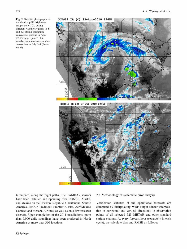
Figure 2 shows examples of the typical weather regimes

during the cool (S1) and warm (S2) seasons. The S1 period

is characterized in a large part by the passage of frontal

systems during the winter and spring seasons, while the S2

period is characterized by convective activities during the

summer and early fall.

Finally, it is noted here that one of the unique datasets

assimilated in the NCAR-AirDat WRF-RTFDDA system is

the AirDat TAMDAR observation. TAMDAR is an air-

borne multi-function in situ atmospheric sensor equipped

on commercial aircrafts, and provides measurements

of humidity, pressure, temperature, winds, icing, and

Table 1 List of NCAR-AirDat WRF-RTFDDA model physical

parameterization and configuration

Physics Scheme

Nested-grid One-way

Time integration Adaptive time step

Land surface Noah

Surface layer Monin–Obukhov

PBL YSU (non-local mixing)

SW-RAD Dudhia

LW-RAD RRTM

Clod microphysics Lin et at.; Morrison (from December 17, 2009)

Cumulus scheme Kain–Fritsch (12 km only)

Analysis of the surface temperature and wind forecast errors 127

123

turbulence, along the flight paths. The TAMDAR sensors

have been installed and operating over CONUS, Alaska,

and Mexico on the Horizon, Republic, Chautauqua, Shuttle

America, PenAir, Piedmont, Frontier Alaska, AeroMexico

Connect and Mesaba Airlines, as well as on a few research

aircrafts. Upon completion of the 2011 installations, more

than 6,000 daily soundings have been produced in North

America at more than 360 locations.

2.3 Methodology of systematic error analysis

Verification statistics of the operational forecasts are

computed by interpolating WRF output (linear interpola-

tion in horizontal and vertical directions) to observation

points of all selected 523 METAR and other standard

surface stations. At every forecast hour (separately in each

cycle), we calculate bias and RMSE as follows:

Fig. 2 Satellite photographs of

the cloud top IR brightness

temperature (�C), during

different weather regimes in S1

and S2: strong springtime

convective systems in April

22–25 (upper panel); fair-

weather summer-time cumulus

convection in July 6–9 (lower

panel)


123

BIAS ¼ 1=N

XN

i¼1

CfðiÞ � COðiÞð Þ ð1Þ

RMSE ¼

ffiffiffiffiffiffiffiffiffiffiffiffiffiffiffiffiffiffiffiffiffiffiffiffiffiffiffiffiffiffiffiffiffiffiffiffiffiffiffiffiffiffiffiffiffiffiffiffi

1=N

XN

i¼1

CfðiÞ � COðiÞð Þ2vuut ; ð2Þ

wherein N is the number of all valid observations, CO is the

observed meteorological quantity at a station location and

at a particular time, and Cf is the model prediction at the

same time interpolated to the same location. The bias is

defined here as the ‘‘difference of the central location of the

forecasts and the observations’’ (Jolliffe and Stephenson

2011). The RMSE is generally more sensitive to large

errors because the square power provides more weight to

the larger error values. On the other hand, the mean bias

does not reflect positive and negative errors for individual

cases because they tend to cancel out. The standard

deviations of the BIAS (STDBIAS) and RMSE (STDRMSE)

as well as correlation skill score COR are also computed as

STDBIAS ¼

ffiffiffiffiffiffiffiffiffiffiffiffiffiffiffiffiffiffiffiffiffiffiffiffiffiffiffiffiffiffiffiffiffiffiffiffiffiffiffiffiffiffiffiffiffiffiffiffiffiffiffiffiffiffiffiffiffiffiffiffiffiffiffiffiffiffiffiffiffiffiffiffiffiffiffiffi

1=ðN � 1ÞXN

i¼1

CfðiÞ � COðiÞ � BIASð Þ2vuut

ð3Þ

STDRMSE ¼

ffiffiffiffiffiffiffiffiffiffiffiffiffiffiffiffiffiffiffiffiffiffiffiffiffiffiffiffiffiffiffiffiffiffiffiffiffiffiffiffiffiffiffiffiffiffiffiffiffiffiffiffiffiffiffiffiffiffiffiffiffiffiffiffiffiffiffiffiffiffiffiffiffiffiffiffiffiffiffi

1=ðN � 1ÞXN

i¼1

CfðiÞ � COðiÞ � RMSEð Þ2vuut

ð4Þ

CORR ¼ covðCf ;COÞ=ffiffiffiffiffiffiffiffiffiffiffiffiffiffiffiffiffiffiffiffiffiffiffiffiffiffiffiffiffiffiffiffivarðCfÞvarðCOÞ

pð5Þ

The correlation skill score (CORR) evaluates systematic

relations between forecasts and observations, for example,

their error differences and the amplitudes. Thus, perfect

correlation exists for COR = 1 or COR = -1. STDBIAS

indicates the variability of random errors relative to the

bias, similarly, STDRMS to the mean RMSE.

3 Spatiotemporal variations of the forecast biases

The investigation of model biases and their characteristics

have been the subject of several recent publications. For

example, Cheng and Steenburgh (2005) and Molders (2008)

showed a general tendency of the WRF model (Skamarock

et al. 2005) to overestimate the 10-m wind speed over the

western part of US and Alaska, respectively. The large-

magnitude bias in wind speed and wind direction was also

identified in recent versions of WRF in simulations over

mountainous areas (Roux et al. 2009; Mass and Ovens 2011;

Jimenez and Dudhia 2012, 2013). The studies of Prabha and

Hoogenboom (2008) and Liu et al. (2009) reported the

underestimation of the 2-m daytime temperature, with

average cold biases between -4 and -2 �C. In contrast,

daytime warm biases were noted by Coleman et al. (2010) in

their summertime simulations over the Los Angeles basin

using the WRF model, as well as the fifth-generation Penn-

sylvania State University—NCAR Mesoscale Model (MM5;

Grell et al. 1994). Coleman et al. (2010) attributed the day-

time warm biases to insufficient representation of the

anthropogenic latent heat flux, a source of enthalpy, resulting

in significant cooling in the planetary boundary-layer (PBL)

schemes. More recently, in the springtime-2011 15- and

3-km WRF-CONUS simulations Romine et al. (2013)

reported the diurnal and synoptic-scale variability in the

temperature mean errors, positive bias in 2-m dewpoint, and

wind-direction errors related to the synoptic variability

within the model domain. In this section, we analyze the

forecast errors of the 2-m temperatures and 10-m winds of

the NCAR-AirDat 4-km WRF-RTFDDA system for an

operational period of 14 months. All available forecast

cycles during the period are included in the study.

3.1 Domain-averaged error characteristics

Figure 3 illustrates the domain-averaged RMSE and stan-

dard deviation of the 24 h forecasts of 2-m temperature,

10-m wind speed and wind direction for the four forecast

cycles (00, 06, 12, 18 UTC) averaged over the entire S1

period. The averaging is done for all available forecast

cycles between 1 July, 2009 and 22 April, 2010. The

temperature errors exhibit strong diurnal patterns in each

cycle with a growing trend during the daytime and peaking

in the late afternoon. There is a period of approximately

3 h following the late afternoon peak when the temperature

error decreases, and then stays roughly constant during the

nighttime. The standard deviation of the RMSE around the

mean values is moderate and never exceeds 0.4 K for

temperature and 0.3 m s-1 for wind speed. On average, the

temperature errors for the 00 UTC cycle are lower than

those of the other cycles, which may be attributable to the

assimilation of more aircraft data of the daytime flights and

RAOB data, as noted by Croke et al. (2010). The minimum

error of 1.8 K is always found at the end of the analysis

time (or the 0-h forecast lead time) for all the cycles, which

is most likely due to the effect of continuous assimilation.

The maximum error in 2-m temperature reaches 2.5 K.

Roux et al. (2009) also showed a strong effect of the

diurnal cycle on the model-forecast bias, with maximum

temperature errors increasing from 1.8 K during the ana-

lysis period to 2.5 K at the late afternoon hours.

In comparison, the diurnal variability in 10-m wind

speed error and 10-m wind-direction error are less pro-

nounced when compared to those of 2-m temperature

(Fig. 3). For wind speed, nighttime and early morning

correspond to relatively smaller errors while relatively


123

larger errors on the order of 1.9 m s-1 are found around

noon. For wind direction, the error distributions appear to

be out of phase with those of wind speed. The spread of the

RMSE around the mean is small for wind speed

(\0.3 m s-1), but is quite large for wind direction (*50�).

Figure 4 presents the domain-averaged RMSE as a func-

tion of 0 to 72-h forecast lead time averaged over the entire

S2 period. Increasing trends in the RMSEs of temperature,

wind speed, and wind direction with forecast lead time are

evident (especially for temperature), with superposed strong

diurnal variations. The maximum temperature errors that

peak in late afternoon grow from 2.5 K in the beginning of

the forecast cycle to 3.2 K at the end of the forecast cycle. As

in the S1 period, the largest wind-speed errors occur around

noon, and grow from 1.9 to 2.1 m s-1 during the 72-h

forecast length. Averaged over the entire CONUS domain,

the 10-m wind-speed daytime bias is about 0.5 m s-1 while

the MAE of 10-m wind speeds grows gradually from

approximately 1.2 m s-1 during the analysis period to

2 m s-1 at the end of the 72-h forecast length (not shown).

Compared to the findings of the other regional models

reported in literatures, the NCAR-AirDat CONUS WRF-

RTFDDA system shows slightly better forecast verification

statistics. Case et al. (2002) evaluated high-resolution

(1.25-km grid spacing) simulations of the Regional

Atmospheric Modeling System (RAMS) over east-central

Florida during the 1999 and 2000 summer months. They

showed that the temperature and wind-speed RMSE for a

24-h forecast corresponding to the 12 UTC cycle had very

similar temporal structure to the current results. Their peak

temperature (wind speed) RMSE reached 3.75 K

(2.5 m s-1) at the end of the 9-h (7-h) forecast. In com-

parison, the NCAR-AirDat system has a peak temperature

(wind speed) RMSE of 2.5 K (1.9 m s-1) at the end of 6-h

(12-h) forecast for the 12 UTC cycle (see Figs. 3, 4).

Jones et al. (2007) examined the RMSE of the 48-h

MM5 ensemble forecasts over the northeast US at 12-km

horizontal resolution. They showed that the temperature

RMSE approached 2.8 K and increased with the forecast

length, which is similar to the current results. Their wind-

speed RMSE exhibited strong diurnal cycles with errors in

the range of 2–2.8 m s-1, while the current results show

relatively smaller errors in the range of 1.5–2.1 m s-1.

Jones et al. (2007) also showed that the wind-direction

RMSE in their simulations had similar time tendencies to

Case et al. (2002), i.e., increasing from 40� to 55� at the

end of the 48-h forecasts in warm season (May–Septem-

ber), and from 30� to 45� in cool season (October–March).

The WRF-RTFDDA wind-direction RMSE in the current

study consistently exhibits the same time tendency for both

Fig. 3 Domain-averaged RMSE (black lines) and standard deviation

(shadings) of 2-m temperature, 10-m wind speed, and wind-direction

forecasts as a function of 0- to 24-h forecast lead time for each of the

four cycles averaged over the S1 period of July 1, 2009 through April

22, 2010


123

cool and warm seasons, with higher RMSE in the range of

90�–95� within the 72-h forecasts and a daily fluctuation of

±5�. The higher mean RMSE in our WRF-RTFDDA

simulations is likely related to large wind-direction errors

over the Rocky Mountain areas where the model tends to

have a difficulty in resolving the wind direction realisti-

cally due to the complex terrain.

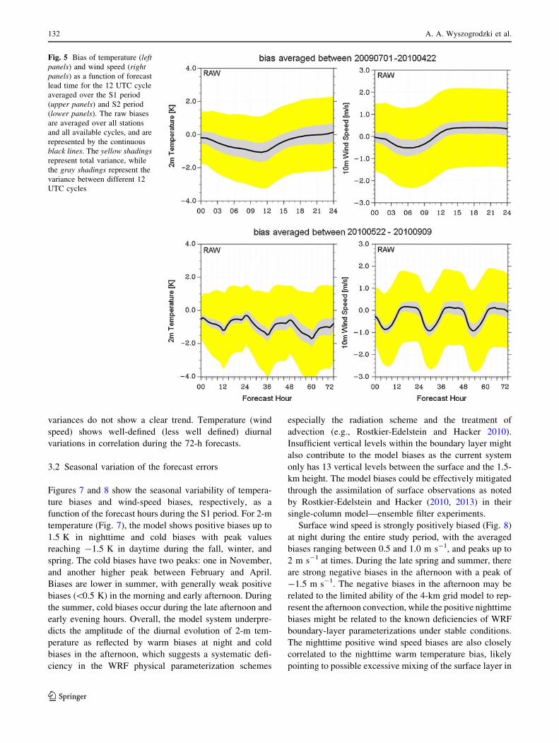
The biases of temperature and wind speed as a function

of forecast lead time averaged over the S1 and S2 periods

for the 12 UTC cycles are presented in Fig. 5. The growth

of temperature and wind-speed RMSE during the first few

hours of the forecasts seen in Fig. 3 appears to be related to

the increasing negative biases of the respective variables

during the same time period (Fig. 5). The averaged maxi-

mum biases reach -1 K for temperature and -0.5 m s-1

for wind speed during the S1 period. At the end of the 24-h

forecasts the average temperature biases decreased to zero

while the total variances (represented by the yellow shad-

ings) increased to ±2 K. The averaged wind-speed biases

stay approximately constant in the second half of the 24-h

forecasts with positive values not exceeding 0.3 m s-1 and

total variances in the range of ±1.3 m s-1. Both the tem-

perature and wind-speed biases during the S2 period show

strong diurnal variations (Fig. 5). The gradual increases of

the averaged negative temperature biases as well as the

total variance correlate well with the gradual increase of

temperature RMSE in Fig. 4. For wind speed, biases stay

nearly unchanged during the 72-h forecasts; however, the

total variances increase slowly and reach ±1.6 m s-1 at the

end of the 72-h forecasts, which also corresponds well to

the gradual increase of wind-speed RMSE seen in Fig. 4.

Figure 6 shows the correlation of temperature and wind

speed between the model forecasts and the observations as

a function of forecast lead time for the 12 UTC cycle.

Apparently, the correlation is much higher for temperature

than wind speed for both S1 and S2 periods. Gradual

decreases in the correlation with the forecast lead time are

noticed for both temperature and wind speed; however, the

Fig. 4 Same as Fig. 3 except for the 0- to 72-h forecast lead time averaged over the S2 period of 22 May 2010 through 9 September 2010


123

variances do not show a clear trend. Temperature (wind

speed) shows well-defined (less well defined) diurnal

variations in correlation during the 72-h forecasts.

3.2 Seasonal variation of the forecast errors

Figures 7 and 8 show the seasonal variability of tempera-

ture biases and wind-speed biases, respectively, as a

function of the forecast hours during the S1 period. For 2-m

temperature (Fig. 7), the model shows positive biases up to

1.5 K in nighttime and cold biases with peak values

reaching -1.5 K in daytime during the fall, winter, and

spring. The cold biases have two peaks: one in November,

and another higher peak between February and April.

Biases are lower in summer, with generally weak positive

biases (\0.5 K) in the morning and early afternoon. During

the summer, cold biases occur during the late afternoon and

early evening hours. Overall, the model system underpre-

dicts the amplitude of the diurnal evolution of 2-m tem-

perature as reflected by warm biases at night and cold

biases in the afternoon, which suggests a systematic defi-

ciency in the WRF physical parameterization schemes

especially the radiation scheme and the treatment of

advection (e.g., Rostkier-Edelstein and Hacker 2010).

Insufficient vertical levels within the boundary layer might

also contribute to the model biases as the current system

only has 13 vertical levels between the surface and the 1.5-

km height. The model biases could be effectively mitigated

through the assimilation of surface observations as noted

by Rostkier-Edelstein and Hacker (2010, 2013) in their

single-column model—ensemble filter experiments.

Surface wind speed is strongly positively biased (Fig. 8)

at night during the entire study period, with the averaged

biases ranging between 0.5 and 1.0 m s-1, and peaks up to

2 m s-1 at times. During the late spring and summer, there

are strong negative biases in the afternoon with a peak of

-1.5 m s-1. The negative biases in the afternoon may be

related to the limited ability of the 4-km grid model to rep-

resent the afternoon convection, while the positive nighttime

biases might be related to the known deficiencies of WRF

boundary-layer parameterizations under stable conditions.

The nighttime positive wind speed biases are also closely

correlated to the nighttime warm temperature bias, likely

pointing to possible excessive mixing of the surface layer in

Fig. 5 Bias of temperature (left

panels) and wind speed (right

panels) as a function of forecast

lead time for the 12 UTC cycle

averaged over the S1 period

(upper panels) and S2 period

(lower panels). The raw biases

are averaged over all stations

and all available cycles, and are

represented by the continuous

black lines. The yellow shadings

represent total variance, while

the gray shadings represent the

variance between different 12

UTC cycles


123

Fig. 6 Correlation coefficients

of the observed and simulated

temperature (left panels) and

wind speed (right panels) as a

function of forecast lead time

for the 12 UTC cycle during the

S1 period (upper panels) and S2

period (lower panels). The mean

and variance are represented by

thick black lines and gray

shadings, respectively

Fig. 7 Temporal variations of

the domain-averaged daily

temperature biases as a function

of forecast lead time for each of

the four cycles during the period

of July 1, 2009 through April

22, 2010 (the S1 period; the

forecast date is written in the

format month/day along the

y axis)


123

the model, which may be in turn due to small-scale terrain

drag that is unresolved by the current weather models (Ste-

eneveld et al. 2008). Steeneveld et al. (2009) showed that

gravity wave drag due to small obstacles, mountains and hills

could reach the equivalent magnitude as the turbulent drag

and could modify the wind speed sufficiently.

The temperature and wind-speed biases as a function of

forecast lead time for the 00 UTC (late afternoon over

CONUS) cycle and 12 UTC (early morning over CONUS)

cycle during the S2 period are shown in Fig. 9. As in the

case for the S1 period, warm (positive) biases in the

nighttime and cold (negative) biases in the afternoon are

evident for temperature (wind speed) during the S2 period.

The daytime cold bias reaches -1.5 K during the late

afternoon hours, while the nighttime warm bias is generally

less than 0.3 K. The wind speed tends to be under-pre-

dicted by -1.5 m s-1 in the afternoon. Between the late

afternoon (i.e., 00 UTC) cycle and the early morning (i.e.,

12 UTC) cycle, relatively small differences are noticed for

wind speed during the entire S2 period; however, the

temperature biases exhibit significant differences espe-

cially during June, July, and August (Fig. 9). The tem-

perature biases from May to early June and from late

August to September are greater than those in the other

months for both cycles. Spring weather over CONUS is

characterized by substantial increases in temperature and

wind speed with a gradual decrease in precipitation, while

in the autumn and winter, the weather conditions are nearly

the opposite. In the summer, unstable conditions with

convective activities dominate the weather over CONUS.

Thus, it appears that the seasonal changes in the forecast

biases more or less reflect the model’s varying skills under

different weather regimes, for example, treatment of shal-

low cumulus convection (e.g., Angevine 2005; Angevine

et al. 2010).

The mean RMSE of the S1 and S2 periods seen in

Figs. 3 and 4 contains both systematic (i.e., bias) and

random-error components. The variance, also known as the

Fig. 8 Same as Fig. 7 except

for the domain-averaged daily

wind-speed biases


123

centered root-mean square error (CRMSE2), is the random

component defined as follows,

CRMSE2 ¼ 1=N

XN

i¼1

ðCfðiÞ � �CfÞ � ðCOðiÞ � �COÞ½ �2

¼ RMSE2 � BIAS2 ð6Þ

and is partly caused by the under-resolved small-scale or

high-frequency phenomena such as convective cells by the

4-km grid model. The mean RMSE in the S2 period (Fig. 4)

shows a much stronger diurnal signature than that in the S1

period (Fig. 3) and the most likely reason is that the mean

RMSE in the S1 period is obtained by averaging across

multiple seasons with differing diurnal bias distributions.

3.3 Error geographical distributions

Figure 10 displays the geographical distributions of the

mean bias of 10-m wind speed, 10-m wind direction and

2-m temperature for the 00 UTC (late afternoon) and 12

UTC (early morning) cycles. The biases are computed for

the 24-h forecasts, and the averaging is done for all forecast

cycles of the S1 period. The wind-speed forecasts for the

stations in the western portion of the domain, mostly along

the slopes of the Rocky Mountains and in the Central

Valley of California, have large negative biases at 00 UTC,

some as low as -3 m s-1. The wind-speed biases are

smaller at most coastal mountainous locations at 12 UTC.

In contrast, positive wind-speed biases of up to 2 m s-1

can be seen in the eastern coastal areas, as well as the

northwestern coastal areas, including northern California,

Oregon, and Washington for both cycles. Stations in the

Midwest including the Great Plains exhibit relatively

smaller wind-speed biases for both cycles.

The wind-direction biases show irregular distributions in

the eastern areas with large variations among stations. The

biases, however, are strongly negative (counterclockwise)

over the Rocky Mountains with values reaching -25 �, and

Fig. 9 Temporal variations of

the domain-averaged daily

temperature biases (upper

panels) and wind-speed biases

(lower panels) as a function of

forecast lead time for the 00

UTC cycle (late afternoon, left

panels) and 12 UTC cycle (early

morning, right panels) during

the period of May 22, 2010

through September 9, 2010 (the

S2 period)


123

Fig. 10 Geographical distribution of biases for the S1 period: 00 UTC (left panels) and 12 UTC (right panels). The biases of the 24-h forecasts

are averaged over all valid cycles within S1


123

positive biases of up to 20 � are observed along the western

Rocky Mountain slopes for the 00 UTC cycle. Further-

more, the wind-direction biases on the slopes are about 5 �greater for the 12 UTC cycle when compared to the 00

UTC cycle. The wind-direction biases in the mountainous

regions may indicate some deficiencies in the model’s

representation of the topographic forcing, which likely

causes systematic flow shifts. In WRF simulations over the

Pacific Northwest at the 12-km grid spacing, Mass and

Ovens (2011) also noted over-prediction of the near-sur-

face wind speed and wind-direction errors at low levels in

areas of complex terrain in which the flow tends to be too

geostrophic. They attributed the causes of the model errors

to the lack of sub-grid terrain friction in WRF and subse-

quently introduced an algorithm to mitigate the errors in

wind speed and direction.

The temperature biases also exhibit notable spatial

variations between the east states and the west states

(Fig. 10). Some large cold biases up to -4.0 K occur over

the Appalachian Mountains, the valleys of California and

Washington, and over the Rocky Mountains for the 00

UTC cycle. The Northern and Southern Plains show neg-

ligible biases for the 00 UTC cycle, but warm biases up to

1.5 K for the 12 UTC cycle. Compared to the 00 UTC

cycle, the 12 UTC cycle shows mainly positive biases over

CONUS, except for a region along the Appalachian range

where negative biases in the range of -1.5 K are found.

The larger daytime cold biases associated with the high

mountains for the 00 UTC cycle constitute a complicated

modeling challenge. The causes of the larger biases may be

related to (a) imperfect atmospheric radiation transfer over

the high terrain; (b) inaccurate representation of the land-

use properties; (c) truncated valleys/peaks of mountain

ranges due to limited model grid resolution; (d) inaccurate

mountainous cloud simulation; and (or) (e) uncertainty in

the model surface-snow process parameterization within

the land-surface model (LSM) (e.g., Barlage et al. 2010;

Mass and Owens 2013). An increasing trend in removing

these error sources from the NWP systems are currently

observed in the modeling community.

Barlage et al. (2010) introduced a time-varying albedo

formulation that increases the fresh snow albedo in the

WRF-Noah LSM and improves the magnitude and timing

of seasonal maximum snow-water equivalent (SWE) in the

Colorado Rocky Mountains. Minor improvements in the

averaged SWE were also obtained by introducing adjust-

ments to surface exchange coefficients in the stable

boundary layer, as well as the surface roughness length

over snow. The same authors also found that introduction

of terrain orientation and slope dependence did not affect

the simulated SWE seasonal maximum; however, the

diurnal distributions of incoming solar radiation between

the east- and west-facing slopes were changed. These

changes between the slopes might affect the convective

precipitation, accumulation and ablation of snow, and

hence, directly change the distributions and amplitude of

the temperature biases along the mountain ranges.

Biases in coastal areas are affected by the different

diurnal land–water heating, and are subjected to the

imperfect simulations of the magnitude and phases of sea

and land breezes. Notice that in the current study, the

nighttime warm biases in the coastal areas nearly disappear

during the daytime. Croke et al. (2010) suggested that the

diurnal signal in the temperature biases is linked to the

nocturnal damping of the sea breezes by the warm coastal

waters in the fall. Case et al. (2008) investigated improve-

ments in the land-surface initialization of the WRF model

using NASA Land Information System (LIS) conditions.

The drier initial soil states in their simulations improved the

simulation of the timing and evolution of a sea breeze over

northwestern Florida, which resulted in a reduction in both

the nocturnal warm bias, as well as the daytime cold bias.

4 Correlation of forecast biases terrain heights

Complex terrain significantly impacts weather systems that

pass by and greatly modulates the local and regional weather

processes as reported by Roux et al. (2009) and Mass and

Ovens (2011) in the recent versions of WRF over the North-

west Pacific area. More recently, Jimenez and Dudhia (2012)

showed positive bias (*1 ms-1) over the valleys and plains

and large negative bias (-3 m s-1) at the hills and mountains.

On average, both biases are compensated although the uneven

sampling of the wind by the larger number of stations located

in plains and valleys comparing to number of mountain sta-

tions results in an overall positive bias. Jimenez and Dudhia

(2013) also found large magnitude of biases of the wind

direction (RMSE of 80�) over the areas of complex terrain and

these errors were dependent inversely on the surface wind

speed. In this section, we present detailed analyses of the

model biases in the context of terrain including their seasonal

variability and the terrain dependency.

4.1 Seasonal bias variability for the lower

and the higher elevation stations

Figure 11 shows the distributions of the mean temperature

bias for all 12 UTC forecast cycles in the S1 period aver-

aged both over all stations and over stations with terrain

heights either above or below 600 m above seal level

(ASL). The 600-m threshold was chosen arbitrarily with

the purpose of distinguishing the low-altitude coastal areas

from the high plains and mountains. The results indicate

that the high-elevation stations have much larger warm

biases during the nighttime with maxima exceeding 1.5 K,


123

and cold biases during the daytime ([-1.5 K). The

nighttime warm biases are much greater in the winter than

the other seasons during the S1 period. During the summer,

convection that frequently occurs in the afternoon may lead

to a decrease of the nighttime warm biases. This appears to

be the case especially for the low-elevation stations

(Fig. 11). As a matter of fact, even the western stations

exhibit small cold biases at night (not shown).

The low-elevation stations tend to show cold biases for

both the daytime and nighttime for the reasons discussed

above; however, the amplitude of the cold biases exhibits

strong seasonal dependence. For example, in the summer,

the daytime negative biases are normally greater than

-0.8 K; but in the spring, the cold biases in the daytime

could reach as high as -1.4 K. At the nighttime, slightly

negative biases in the range of -0.3 K exist during the

spring and summer, with peak values around -1.0 K

during the middle of June. During December and January,

the negative biases are replaced by positive biases and the

maximum values could reach 1.2 K. The negative biases,

seen in Fig. 10, for the eastern stations are then consistent

with the domain-averaged biases for the stations below

600 m, which are around -0.2 K. The small magnitude of

this domain-averaged negative bias is due to the dominance

of the coastal stations located in Florida and North Carolina

for which small positive biases are found.

4.2 Dependence of biases with terrain height

for different forecast cycles

To further analyze the dependence of biases on the terrain

height, we divided the surface stations into 11 groups based

on the stations’ elevations: 15–46, 47–99, 100–167,

168–233, 234–287, 288–396, 397–579, 580–1,004,

1,005–1,481, 1,482–2,117, 2,118 m and higher. Coinci-

dently, each group contains approximately the same num-

ber of stations.

Figure 12 shows the 2-m temperature biases as a func-

tion of the terrain elevation averaged over the S1 period.

The low-elevation stations always show weak cold biases,

regardless of the cycles, with smaller biases at nighttime

(i.e., roughly -0.2 K for the 12 UTC cycle). All stations

exhibit cold biases for the 00 UTC and 18 UTC cycles

while the stations above 400 m for the 12 UTC cycle and

above 600 m for the 06 UTC cycle show warm biases.

Thus, at the higher elevations ([600 m), the temperature

biases display well-defined diurnal variability, with

strongly negative bias (up to -2.0 K) in the daytime (18

and 00 UTC cycles) but moderately positive (up to 1.0 K)

at night. The largest temperature biases are found for the

highest elevations, which is also consistent with the find-

ings in other mesoscale model experiments. For example,

Xu et al. (2009) examined the WRF-ARW model biases in

the complex terrain of Southwest Asia from 1 to 31 May

2006. The 2-m temperature errors in their simulations were

closely related to the heterogeneity in terrain structure,

with larger forecast errors located in the higher elevation

terrain.

The bias distributions presented in Fig. 12 are also

consistent with the individual cycle-averaged results shown

in Fig. 10, showing that the strongest cold biases exist over

the Appalachian Mountains in the eastern part of the model

domain where the average elevation is roughly 900 m with

peaks around 2,100 m. In this elevation range, the largest

cold biases come from the 00 UTC cycle and range from

-1.5 to -4.0 K. Above 2,100 m (the Rocky Mountain

Fig. 11 Mean temperature biases in the S1 period as a function of forecast lead time averaged over all stations (left panel), over stations with

terrain height above 600 m (center panel) and over stations with terrain height below 600 m (right panel) for the 12 UTC cycles


123

stations), the average cold biases are the biggest during the

daytime but shift to weak warm biases during the night;

however, large spatial variations of biases are also evident

within this elevation range. During the daytime, the sta-

tions with small cold biases are located mostly in the

central part of the Rocky Mountains, and larger cold biases

are present in the eastern and western parts of the Rockies,

as well as near coasts in northern California, Oregon, and

the Cascade Mountains of Washington. The latter may be

related to the amount of moisture carried from the Pacific

Ocean deep into the continental areas, as well as the

imperfect representation of the convective cloud processes

along the slopes of this complex topography. The localized

over-prediction of precipitation on the windward slopes

and over the broader leeward regions along the Oregon

Cascades was observed with MM5 (Garvert et al. 2005a, b)

and the Canadian Global Environmental Multiscale (GEM)

model (Milbrandt et al. 2008) model. Lin and Colle (2009)

reported over-prediction of snow by the WRF model along

the Cascades’ windward slopes due to the over-predicted

maximum snow depositional growth, which resulted in

rapid and excessive graupel (rimed snow) fallout.

The model wind directions (Fig. 13) exhibit negative

biases of approximately -9� for the stations with eleva-

tions below 600 m ASL. The smallest wind-direction

errors are seen for the stations with altitudes between 600

and 1,000 m, while the highest errors are found at the

highest stations with elevation in excess of 2,100 m. The

biases from forecast cycles 06 and 12 UTC, which repre-

sent the nocturnal and early morning conditions, show

similar structure with a positive bias of 4� for stations

located between 600 and 1,000 m, 11� for stations

1,500–2,100 m, a negative bias of -12� for stations

1,000–1,500 m, and the largest negative bias of -20� for

the highest stations situated above 2,100 m. The 00 UTC

afternoon forecasts show strong negative biases for stations

located above 1,000 m, reaching -20� at the highest sta-

tion locations. The mid-day forecast conditions from the 18

UTC cycles produce small biases for station elevations

between 600 and 2,100 m, and positive biases of up to 8�for the highest station locations.

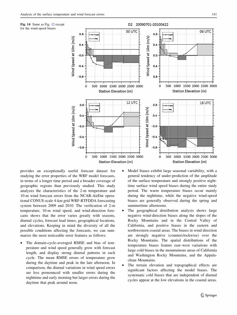
The 10-m wind-speed biases presented in Fig. 14 show

an interesting difference between the mid-elevation sta-

tions with consistently negative biases, and the low- and

Fig. 12 Temperature biases as

a function of the terrain

elevation averaged over the S1

period. The dashed-dot lines are

the averaged biases for all

stations higher than the

elevation threshold. The

continuous horizontal lines are

the average over all station

elevations


123

high-elevation stations where the bias sign changes

between cycles. Strong diurnal variability is seen at the

higher elevation stations located above 2,100 m, changing

from a negative daytime bias of -0.8 m s-1 to positive

biases with a peak of 0.6 m s-1 during the early morning

hours. The cycle-averaged biases in wind speed are small

at many stations (see Fig. 10), and are most likely due to

the cancellation of the positive and negative biases

throughout the diurnal cycle. This is especially true for the

majority of the Rocky Mountain stations. The biases at

middle elevation stations between 1,000 and 2,100 m

remain negative with a nocturnal minimum of -0.3 m s-1

and mid-day negative peak of -0.8 m s-1. The average

negative wind-speed bias in Fig. 8 is the combined signa-

ture of the stations in the Great Plains, the California

Coastal Range, and several stations with a weaker negative

bias in the Rocky Mountains. At the low elevations, the

biases are mostly positive with a maximum of 0.7 m s-1,

except during the middle of the day when the biases

become negative at each model elevation. When averaged

across all cycles, the low-elevation stations indicate strong

positive biases with the highest positive bias near the

coastal locations, as well as stations around the Appala-

chian Mountains.

The nighttime wind-speed biases presented here are in

agreement with the results provided by Roux et al. (2009)

who also found that the wind-speed biases decreased from

lower terrain to about 600 m ASL, and then increased with

elevation toward the mountain peaks. The same authors

noted that the lowest biases were seen at stations between

400 and 1,500 m ASL while the highest biases were

identified at stations located near sea level and the higher-

altitude mountains. This observation calls for future

research on stable boundary-layer parameterizations over

large mountain ranges.

5 Summary

Investigating the characteristics of model-forecast errors

using various statistical and object-oriented methods is

necessary for providing useful guidance to end-users and

model developers as well. The NCAR-AirDat weather

research and forecasting (WRF)-based real-time four-

dimensional data assimilation (RTFDDA) and forecasting

system, running operationally over a contiguous United

States (CONUS) domain at a 4-km grid spacing with four

forecast cycles daily from June 2009 to September 2010,


for the wind-direction biases


123

provides an exceptionally useful forecast dataset for

studying the error properties of the WRF model forecasts,

in terms of a longer time period and a broader coverage of

geographic regions than previously studied. This study

analyzes the characteristics of the 2-m temperature and

10-m wind forecast errors from the NCAR-AirDat opera-

tional CONUS-scale 4-km grid WRF-RTFDDA forecasting

system between 2009 and 2010. The verification of 2-m

temperature, 10-m wind speed, and wind-direction fore-

casts shows that the error varies greatly with seasons,

diurnal cycles, forecast lead times, geographical locations,

and elevations. Keeping in mind the diversity of all the

possible conditions affecting the forecasts, we can sum-

marize the most noticeable error features as follows:

• The domain-cycle-averaged RMSE and bias of tem-

perature and wind speed generally grow with forecast

length, and display strong diurnal patterns in each

cycle. The mean RMSE errors of temperature grow

during the daytime and peak in the late afternoon. In

comparison, the diurnal variations in wind speed errors

are less pronounced with smaller errors during the

nighttime and early morning but larger errors during the

daytime that peak around noon.

• Model biases exhibit large seasonal variability, with a

general tendency of under-prediction of the amplitude

of the surface temperature and strongly positive night-

time surface wind speed biases during the entire study

period. The warm temperature biases occur mainly

during the nighttime, while the negative wind-speed

biases are generally observed during the spring and

summertime afternoons.

• The geographical distribution analysis shows large

negative wind-direction biases along the slopes of the

Rocky Mountains and in the Central Valley of

California, and positive biases in the eastern and

northwestern coastal areas. The biases in wind direction

are strongly negative (counterclockwise) over the

Rocky Mountains. The spatial distributions of the

temperature biases feature east–west variations with

large cold biases in the mountainous areas of California

and Washington Rocky Mountains, and the Appala-

chian Mountains.

• The terrain elevation and topographical effects are

significant factors affecting the model biases. The

systematic cold biases that are independent of diurnal

cycles appear at the low elevations in the coastal areas.


for the wind-speed biases


123

At higher elevations with terrain height in excess of

600 m ASL, the cold (warm) biases are seen only

during the daytime (nighttime). The highest wind speed

errors are found over high terrain (mostly negative

biases) and near sea-level stations (mostly positive

biases). The negative temperature biases exist at all

elevations around noontime. At elevations between

1,000 and 2,100 m, negative wind-speed biases with

variable amplitudes during different weather conditions

and forecast duration are identified for each cycle.

Wind-direction errors, largest in the Rocky and Appa-

lachian mountain ranges and in the western coastal

areas, display strong diurnal and spatial variations.

This paper is focused primarily on analysis of the char-

acteristics of the model-forecast errors. The error features

suggest that the model physical parameterization schemes

and model dynamic formulations behave differently

according to the time of the day, seasons, and geographical

(topography and land uses) contrasts. Additional work is

necessary to better understand and identify the sources of

these errors to improve the model forecasts. It is our hope

that the current study could help inform the end-users in

assessing the level of forecast errors in their own use of the

NWP system, and meanwhile, provide the model develop-

ers insight into the behavior of the model-forecast error

dependency given the complex sets of parameterizations.

Acknowledgments The authors are very grateful to NCAR for the

technical and computer support. The comments and suggestions

provided by Jason Knievel and Karen Griggs are greatly appreciated.

NCAR is sponsored by the National Science Foundation.

Open Access This article is distributed under the terms of the

Creative Commons Attribution License which permits any use, dis-

tribution, and reproduction in any medium, provided the original

author(s) and the source are credited.

References

Angevine WM (2005) An integrated turbulence scheme for boundary

layers with shallow cumulus applied to pollutant transport.

J Appl Meteorol 44:1436–1452

Angevine WM, Jiang H, Mauritsen T (2010) Performance of an eddy

diffusivity mass flux scheme for shallow cumulus boundary

layers. Mon Weather Rev 138:2895–2912

Barlage M, Chen F, Tewari M, Ikeda K, Gochis D, Dudhia J,

Rasmussen R, Livneh B, Ek M, Mitchell K (2010) Noah land-

surface model modifications to improve snowpack prediction in

the Colorado Rocky Mountains. J Geophys Res 115:D22101.

doi:10.1029/2009JD013470

Case JL, Manobianco J, Dianic AV, Wheeler MM, Harms DE, Parks

CR (2002) Verification of high-resolution RAMS forecasts over

east-central Florida during the 1999 and 2000 summer months.

Weather Forecast 17:1133–1151

Case JL, Crosson WL, Kumar SV, Lapenta WM, Peters-Lidard CD

(2008) Impacts of high-resolution land surface initialization on

regional sensible weather forecasts from the WRF model.

J Hydrometeorol 9:1249–1266. doi:10.1175/2008JHM990.1

Chen F, Warner TT, Manning K (2001) Sensitivity of orographic

moist convection to landscape variability: a study of the Buffalo

Creek, Colorado, flash flood case of 1996. J Atmos Sci 58:3204–

3223

Cheng WYY, Steenburgh WJ (2005) Evaluation of surface sensible

weather forecasts by the WRF and the eta models over the

Western United States. Weather Forecast 20:812–821

Childs, P, Jacobs N, Croke M, Huffman A, Liu Y, Wu W, Roux G, Ge

M (2010) An introduction to the NCAR-AirDat operational

TAMDAR-enhanced RTFDDA WRF-ARW. In: 14th Sympo-

sium on Integrated Observing and Assimilation Systems for

Atmosphere, Oceans, and Land Surface (IOAS-AOLS), Jan

17–23 2010, Atlanta, Paper 8.4

Coleman RF, Drake JF, McAtee MD, Belsma LO (2010) Anthropo-

genic moisture effects on WRF summertime surface temperature

and mixing ratio forecast skill in Southern California. Weather

Forecast 25:1522–1535

Croke M, Jacobs NA, Childs P, Huffman A, Liu Y, Liu Y, Sheu R-S

(2010) Preliminary verification of the NCAR-Airdat operational

RTFDDA-WRF system. In: 14th Symposium on Integrated

Observing and Assimilation Systems for the Atmosphere,

Oceans, and Land Surface (IOAS-AOLS), AMS, 17–23 Jan

2010, Atlanta, Paper 8.5

Fritsch JM Jr, Houze RA, Adler R, Bluestein H, Bosart L, Brown J,

Carr F, Davis C, Johnson RH, Junker N, Kuo Y-H, Rutledge S,

Smith J, Toth Z, Wilson JW, Zipser E, Zrnic D (1998)

Quantitative precipitation forecasting: report of the eight

prospectus team, US weather research program. BAMS 79:285–

299

Garvert MF, Colle BA, Mass CF (2005a) The 13-14 December 2001

IMPROVE-2 event. Part I: synoptic and mesoscale evolution and

comparison with a mesoscale model simulation. J Atmos Sci

62:3474–3492

Garvert MF, Woods CP, Colle BA, Mass CF, Hobbs PV, Stoelinga

MT, Wolfe JB (2005b) The 13-14 December 2001 IMPROVE-2

event. Part II: comparisons of MM5 model simulations of clouds

and precipitation observations. J Atmos Sci 62:3520–3534

Grell G, Dudhia J, Stauffer DR (1994) A description of the fifth-

generation Penn State/NCAR mesoscale model (MM5). NCAR

Tech. Note NCAR/TN-398 ? STR, National Center for Atmo-

spheric Research, p 117

Hahn RS, Mass CF (2009) The impact of positive-definite moisture

advection and low-level moisture flux bias over orography. Mon

Weather Rev 137:3055–3071

Holt TR, Niyogi D, Chen F, Manning K, LeMone MA, Qureshi A

(2006) Effect of land-atmosphere interactions on the IHOP

24–25 May 2002 convection case. Mon Weather Rev 134:113–

133

Jimenez PA, Dudhia J (2012) Improving the representation of

resolved and unresolved topographic effects on surface wind in

the WRF model. J Appl Meteor Climatol 51:300–316

Jimenez PA, Dudhia J (2013) On the ability of the WRF model to

reproduce the surface wind direction over complex. J Appl

Meteor Climatol. doi:10.1175/JAMC-D-12-0266.1

Jolliffe IT, Stephenson DB (2011) Forecast verification: a practi-

tioner’s guide in atmospheric science. Wiley, London, p 292

Jones MS, Colle BA, Tongue JS (2007) Evaluation of a mesoscale

short-range ensemble forecast system over the Northeast United

States. Weather Forecast 22:36–55

Lin Y, Colle BA (2009) The 4–5 December 2001 IMPROVE-2 event:

observed Microphysics and comparisons with the weather

research and forecasting model. Mon Weather Rev 137:1372–

1392


123

http://dx.doi.org/10.1029/2009JD013470

http://dx.doi.org/10.1175/2008JHM990.1

http://dx.doi.org/10.1175/JAMC-D-12-0266.1

Lin Y, Colle BA (2011) A new bulk microphysical scheme that

includes riming intensity and temperature-dependent ice char-

acteristics. Mon Weather Rev 139:1013–1035

Lin YL, Farley RD, Orville HD (1983) Bulk parameterization of the

snow field in a cloud model. J Clim Appl Meteor 22:1065–1092

Liu Y, Chen F, Warner T, Basara J (2006) Verification of a mesoscale

data-assimilation and forecasting system for the Oklahoma City

area during the joint Urban 2003 field project. J Appl Meteor

Climatol 45:912–929

Liu Y, Jacobs NA, Yu W, Warner TT, Swerdlin SP, Anderson M

(2007) An OSSE study of TAMDAR data impact on mesoscale

data assimilation and prediction. In: 11th Symposium on

Integrated Observing and Assimilation Systems for Atmosphere,

Oceans, and Land Surface (IOAS-AOLS), AMS, 14–18 Jan

2007, San Antonio

Liu Y, Warner TT, Bowers JF, Carson LP, Chen F, Clough CA, Davis

CA, Egeland CH, Halvorson SF Jr, Huck TW, Lachapelle L,

Malone RE, Rife DL, Sheu R-S, Swerdlin SP, Weingarten DS

(2008a) The operational mesogamma-scale analysis and forecast

system of the US Army test and evaluation command. Part I:

overview of the modeling system, the forecast products, and how

the products are used. J Appl Meteor Climatol 47:1077–1092

Liu Y, Warner TT, Astling EG, Bowers JF, Davis CA, Halvorson SF,

Rife DL, Sheu R-S, Swerdlin SP, Xu M (2008b) The operational

mesogamma-scale analysis and forecast system of the US Army

test and evaluation command. Part II: interrange comparison of

the accuracy of model analyses and forecasts. J Appl Meteor

Climatol 47:1093–1104

Liu Y, Warner T, Wu W, Roux G, Cheng W, Liu Y, Chen F, Delle

Monache L, Mahoney W, Swerdlin S (2009) A versatile WRF

and MM5-based weather analysis and forecasting system for

supporting wind energy prediction. In: 23rd WAF/19th NWP

Conference, AMS, Omaha, NE. 1–5 June 2009, Paper 17B.3

Liu Y, Zhang Y, Wu W, Roux G, Ge M, Sheu R-S, Warner T, Jocobs

N, Childs P, Croke M (2010) Evaluation of TAMDAR data

impact on predicting warm-season convection using the NCAR-

AirDat WRF-based RTFDDA system. In: 14th integrated

observing and assimilation systems for the atmosphere, oceans

and land surface (IOAS-AOLS), AMS, Atlanta, GA, 17–23 Jan

2010

Mass CF Ovens D (2013) Strange linear features in WRF clouds and

precipitation: diagnosis and correction. In: 14th Annual WRF

Users’ Workshop, 24–27 June, Boulder, CO. Paper 8.2. http://

www.mmm.ucar.edu/wrf/users/workshops/WS2013/ppts/8.2.pdf

Mass CF, Ovens D (2011) Fixing WRF’s high speed wind bias: a new

subgrid scale drag parameterization and the role of detailed

verification. In: 24th Conference on Weather and Forecasting

and 20th Conference on Numerical Weather Prediction, Pre-

prints, 91st American Meteorological Society Annual Meeting,

23–27 Jan, Seattle, WA. Paper 9B.6. http://ams.confex.com/ams/

91Annual/webprogram/Paper180011.html

Milbrandt JA, Yau MK, Mailhot J, Belair S (2008) Simulation of an

orographic precipitation event during IMPROVE-2. Part I:

evaluation of the control run using a triple-moment bulk

microphysics scheme. Mon Weather Rev 136:3873–3893

Molders N (2008) Suitability of the weather research and forecasting

(WRF) model to predict the June 2005 fire weather for Interior

Alaska. Weather Forecast 23:953–973

Morrison H, Thompson G, Tatarskii V (2009) Impact of cloud

microphysics on the development of trailing stratiform precip-

itation in a simulated squall line: comparison of one and two-

moment schemes. Mon Weather Rev 137:991–1006

Prabha T, Hoogenboom G (2008) Evaluation of the weather research

and forecasting model for two frost events. Comput Electron

Agric 64(2):234–247

Rife DL, Warner TT, Chen F, Astling EA (2002) Mechanisms for

diurnal boundary-layer circulations in the Great Basin Desert.

Mon Weather Rev 130:921–938

Rife DL, Davis CA, Liu Y, Warner TT (2004) Predictability of low-

level winds by mesoscale meteorological models. Mon Weather

Rev 132:2553–2569

Romine GS, Schwartz CS, Snyder C, Anderson JL, Weisman ML

(2013) Model bias in a continuously cycled assimilation system

and its influence on convection-permitting forecasts. Mon

Weather Rev 141:1263–1284

Rostkier-Edelstein D, Hacker JP (2010) The roles of surface-

observation ensemble assimilation and model complexity for

nowcasting of PBL profiles: a factor separation analysis.


Rostkier-Edelstein D, Hacker JP (2013) Impact of flow dependence,

column covariance, and forecast model type on surface-obser-

vation assimilation for probabilistic PBL profile nowcasts.


Roux G, Liu Y, Delle Monache L, Sheu R-S, Warner TT (2009)

Verification of high resolution WRF RTFDDA surface forecasts

over mountains and plains. In: 10th WRF users’ workshop,

20–23 June, 2009, Boulder

Sharman RD, Liu Y, Sheu R-S, Warner TT, Rife DL, Bowers JF,

Clough CA, Ellison EE (2008) The Operational mesogamma-

scale analysis and forecast system of the US Army test and

evaluation command. Part III: forecasting with secondary-

applications models. J Appl Meteor Climatol 47:1105–1122

Skamarock WC, Klemp JB, Dudhia J, Gill DO, Barker DM, Wang W,

Powers JG (2005) A description of the advanced research WRF

Version 2. NCAR Technical Note, NCAR/TN–468 ? (STR),

National Center for Atmospheric Research, Boulder, p 88

Steeneveld GJ, Holtslag AAM, Nappo CJ, van de Wiel BJH, Mahrt L

(2008) Exploring the possible role of small-scale terrain drag on

stable boundary layers over land. J Appl Meteor Climatol

47:2518–2530

Steeneveld GJ, Nappo CJ, Holtslag AAM (2009) Estimation of

orographically induced wave drag in the stable boundary layer

during the CASES-99 experimental campaign. Acta Geophys

57:857–881

Sutton C, Hamill TM, Warner TT (2006) Will perturbing soil

moisture improve warm-season ensemble forecasts? A proof of

concept. Mon Weather Rev 134:3174–3189

Woods CP, Stoelinga MT, Locatelli JD (2007) The IMPROVE-1

storm of 1-2 February 2001. Part III: sensitivity of a mesoscale

model simulation to the representation of snow particle types and

testing of a bulk microphysical scheme with snow habit

prediction. J Atmos Sci 64:3927–3948

Xu J, Rugg S, Byerle L, Liu Y (2009) Weather forecasts by the WRF-

ARW model with the GSI data assimilation system in the

complex terrain areas of Southwest Asia. Weather Forecast

24:987–1008


123

http://www.mmm.ucar.edu/wrf/users/workshops/WS2013/ppts/8.2.pdf

http://www.mmm.ucar.edu/wrf/users/workshops/WS2013/ppts/8.2.pdf

http://ams.confex.com/ams/91Annual/webprogram/Paper180011.html

http://ams.confex.com/ams/91Annual/webprogram/Paper180011.html

analysis of the surface temperature and wind forecast ... · neil jacobs • peter childs ......

Documents