analysis of salt and casing fracture mechanisms during...

SANDIA REPORT

SAND2006-1974 Unclassified Unlimited Release Printed May 2006 Analysis of Salt and Casing Fracture Mechanisms During Cavern Integrity Testing for SPR Salt Caverns

Steven R. Sobolik and Brian L. Ehgartner Prepared by Sandia National Laboratories Albuquerque, New Mexico 87185 and Livermore, California 94550 Sandia is a multiprogram laboratory operated by Sandia Corporation, a Lockheed Martin Company, for the United States Department of Energy’s National Nuclear Security Administration under Contract DE-AC04-94AL85000. Approved for public release; further dissemination unlimited.

2

Issued by Sandia National Laboratories, operated for the United States Department of Energy by Sandia Corporation.

NOTICE: This report was prepared as an account of work sponsored by an agency of the United States Government. Neither the United States Government, nor any agency thereof, nor any of their employees, nor any of their contractors, subcontractors, or their employees, make any warranty, express or implied, or assume any legal liability or responsibility for the accuracy, completeness, or usefulness of any information, apparatus, product, or process disclosed, or represent that its use would not infringe privately owned rights. Reference herein to any specific commercial product, process, or service by trade name, trademark, manufacturer, or otherwise, does not necessarily constitute or imply its endorsement, recommendation, or favoring by the United States Government, any agency thereof, or any of their contractors or subcontractors. The views and opinions expressed herein do not necessarily state or reflect those of the United States Government, any agency thereof, or any of their contractors. Printed in the United States of America. This report has been reproduced directly from the best available copy. Available to DOE and DOE contractors from

U.S. Department of Energy Office of Scientific and Technical Information P.O. Box 62 Oak Ridge, TN 37831 Telephone: (865)576-8401 Facsimile: (865)576-5728 E-Mail: [email protected] Online ordering: http://www.osti.gov/bridge

Available to the public from

U.S. Department of Commerce National Technical Information Service 5285 Port Royal Rd Springfield, VA 22161 Telephone: (800)553-6847 Facsimile: (703)605-6900 E-Mail: [email protected] Online order: http://www.ntis.gov/help/ordermethods.asp?loc=7-4-0#online

3

SAND2006-1974 Unlimited Release Printed May 2006

Analysis of Salt and Casing Fracture Mechanisms During Cavern Integrity Testing for SPR Salt Caverns

Steven R. Sobolik and Brian L. Ehgartner

Geoscience and Environment Center Sandia National Laboratories

P.O. Box 5800 Albuquerque, NM 87185-0751

Abstract

This report presents computational analyses to evaluate the risk of Cavern Certification Testing on casing damage and salt fracturing. This deliverable is performed in support of the U.S. Strategic Petroleum Reserve. Several models have been built utilizing either a 1-cavern or 19-cavern, 30-degree wedge of symmetry as has been used on previous West Hackberry (Ehgartner and Sobolik, 2002) and Big Hill (Park et al., 2005) analyses. Various stages of complexity have been added to each model: mesh generation for both 1-cavern and 19-cavern fields; the inclusion of the small-diameter well going from the surface to the top of the caverns; and the addition of steel casing and cement liners to the well surfaces. A stratigraphy based on the Bayou Choctaw site has been chosen for modeling, and the caverns are modeled as equivalent cylinders to simplify the calculations. Salt dilation, as defined by two separate dilation criteria, has been generated during simulated workover routines and cavern integrity tests, but only for the models that include the steel casing and cement liners. The addition of these features generates the tensile and shear stress conditions in the model necessary to cause stress states that exceed dilation criteria. These predictions have been made using the power law creep model. The results show that the salt can be damaged during high pressure change conditions in the wells and caverns.

4

ACKNOWLEDGEMENTS The authors would like to thank Moo Lee, Allan Sattler, and Tom Pfeifle for their review and support of this work.

5

TABLE OF CONTENTS

TABLE OF CONTENTS.................................................................................................... 5

LIST OF FIGURES ............................................................................................................ 6

LIST OF TABLES.............................................................................................................. 8

1. Introduction............................................................................................................... 9

1.1 Objective ..................................................................................................................9

1.2 Report Organization...............................................................................................10

2. Site Description....................................................................................................... 11

3. Background For This Analysis ............................................................................... 12

4. Analysis Model ....................................................................................................... 17

4.1 Model Description .................................................................................................17

4.2 Stratigraphy............................................................................................................18

4.3 Numerical and Material Models ............................................................................19

4.4 Material Properties.................................................................................................20

4.5 Damage Criteria .....................................................................................................23

5. Results..................................................................................................................... 25

6. Conclusions............................................................................................................. 48

7. References............................................................................................................... 49

6

LIST OF FIGURES

Figure 1. Location of SPR Sites ....................................................................................................10

Figure 2. Cross-Section (SW to NE) Through Bayou Choctaw Cavern Field ..............................11

Figure 3. Well Pressures and Lithostatic Stresses. ........................................................................12

Figure 4. Well Model Geometry....................................................................................................13

Figure 5. Finite element mesh (top) with horizontal cross-section through caverns (bottom). .....14

Figure 6. Computational mesh used for CIT calculations. ............................................................19

Figure 7. Dilation criteria compared to Bayou Choctaw and Big Hill laboratory data. ................24

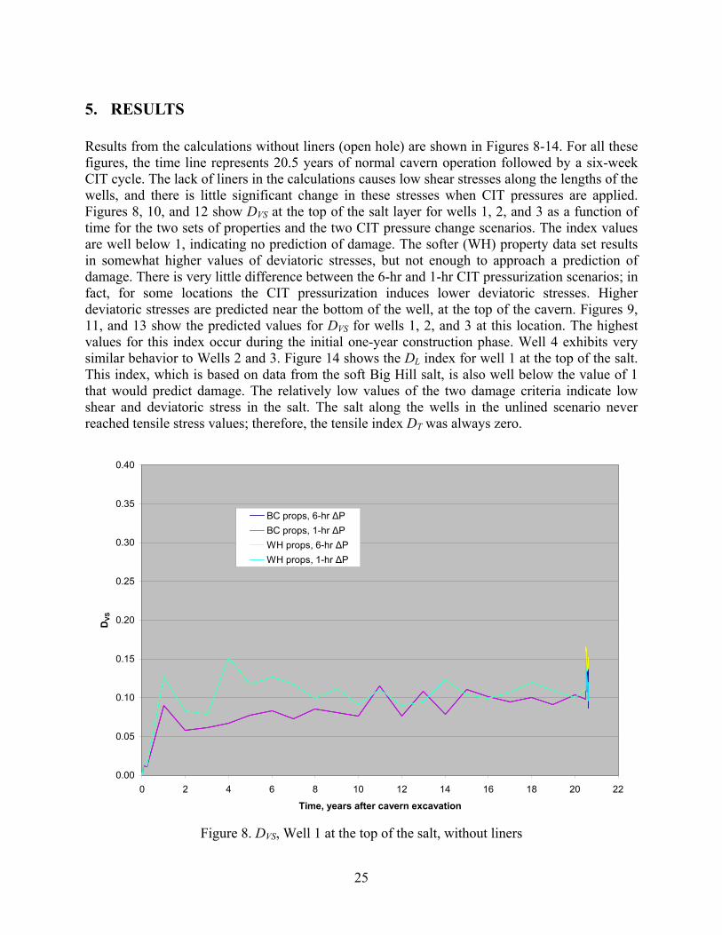
Figure 8. DVS, Well 1 at the top of the salt, without liners.............................................................25

Figure 9. DVS, Well 1 at the bottom of the salt, without liners ......................................................26

Figure 10. DVS, Well 2 at the top of the salt, without liners...........................................................26

Figure 11. DVS, Well 2 at bottom of the salt, without liners ..........................................................27

Figure 12. DVS, Well 3 at the top of the salt, without liners...........................................................27

Figure 13. DVS, Well 3 at bottom of the salt, without liners ..........................................................28

Figure 14. DL, Well 1 at the top of the salt, without liners ............................................................28

Figure 15. DVS, Well 1 at the top of the salt, with liners................................................................30

Figure 16. DVS, Well 1, near the top of the salt, with liners...........................................................30

Figure 17. DVS, Well 1, near the bottom of the salt, with liners.....................................................31

Figure 18. DVS, Well 1 at the bottom of the salt, with liners..........................................................31

Figure 19. DL, Well 1 at the top of the salt, with liners .................................................................32

Figure 20. DL, Well 1 near the bottom of the salt, with liners .......................................................32

Figure 21. DL, Well 1 at the bottom of the salt, with liners ...........................................................33

Figure 22. DT, Well 1 at the top of the salt, with liners .................................................................33

Figure 23. DT, Well 1, near the bottom of the salt, with liners ......................................................34

Figure 24. DVS during CIT, Well 1 at the top of the salt, with liners.............................................35

Figure 25. DVS during CIT, Well 1, near the top of the salt, with liners........................................35

Figure 26. DVS during CIT, Well 1, near the bottom of the salt, with liners..................................36

Figure 27. DVS during CIT, Well 1 at the bottom of the salt, with liners.......................................36




7










Figure 40. Vertical stress in the steel casing, Well 1 .....................................................................43

Figure 41. Vertical stress in the cement liner, Well 1....................................................................44

Figure 42. Vertical view of wells and caverns at times 0, 2 days, 1 and 2 years...........................45

Figure 43. Horizontal displacement in the liners, Well 2, at times 0, 2 days, 1 and 2 years .........46

Figure 44. Horizontal displacement in the liners, Well 2, at times 3, 4, 5, and 20.5 years ...........46

Figure 45. Horizontal displacement along Well 2, unlined well calculations ...............................47

Figure 46. Horizontal displacement along Well 2, lined well calculations ...................................47

8

LIST OF TABLES

Table 1. Cavern and Well Stratigraphy Dimensions Used in CIT Analysis..................................17

Table 2. CIT Pressures as Function of Time................................................................................. 18

Table 3. Power Law Creep Mechanical Properties Used for Salt .................................................21

Table 4. Drucker-Prager constants for anhydrite (Butcher, 1997) ................................................21

Table 5. Material properties of lower caprock (anhydrite) (Butcher, 1997) .................................22

Table 6. Material properties of overburden and upper caprock layers ..........................................22

Table 7. Material properties of the steel casing and cement liner .................................................23

9

1. INTRODUCTION

1.1 OBJECTIVE The U.S. Strategic Petroleum Reserve (SPR) stores crude oil in 62 caverns located at four different sites in Texas (Bryan Mound and Big Hill) and Louisiana (Bayou Choctaw and West Hackberry), shown in Figure 1. The petroleum is stored in solution-mined caverns in salt dome formations. Each cavern is constructed through a well bore that is lined with steel casing and cement from the surface to the top of the cavern. Periodic recertification of the integrity of SPR wells is performed every 5 years using high pressure nitrogen in a procedure known as Cavern Integrity Tests, or CIT. Although the method is very sensitive to leakage of nitrogen through joints in the casing, that leakage has the potential to fracture the salt behind the casing. Above the casing seat, the gas pressures become greater than the lithostatic pressure in the salt. Under these conditions, the potential exists to fracture the salt. Any fracturing of the salt could further precipitate casing failure. Salt fractures can propagate long distances in salt and have resulted in the loss of product at other industrial sites having compromised both the integrity of the cavern and in some cases neighboring caverns. This report presents results from computational analyses to evaluate the risk of Cavern Integrity Testing on casing damage and salt fracturing. This study focuses on the salt portion of the well bore, and examines damage potential to the casings as well as fracture potential to the salt. The potential also exists to fracture the caprock and sand above the salt due to the high gas pressures relative to the in situ stresses; however, above the salt, multiple cemented casings exist, thus making leakage into the formation less likely. Several models have been built utilizing a 19-cavern, 30-degree wedge of symmetry as has been used on previous West Hackberry (Ehgartner and Sobolik, 2002) and Big Hill (Park et al., 2005) analyses. Using those models as a starting point, additional complexity has been added to the computational mesh during the conduct of these analyses, including the addition of the small-diameter well going from the surface to the top of the caverns; and the addition of steel casings and cement liners to the well surfaces. A stratigraphy based on the Bayou Choctaw site has been chosen for modeling, and the caverns are modeled as equivalent cylinders to simplify the calculations. The intent of these calculations is to develop a numerical technique to predict damage in salt, or damage to steel casings and cement liners, utilizing the three-dimensional modeling capabilities of high-performance analytical codes and sophisticated material models. As salt fracturing and casing failures are known to have occurred at underground storage sites similar to SPR, it is necessary to be able to understand the mechanisms involved in salt and casing damage, and to be able to predict such damage under a given set of pressurization and well geometry conditions. In the West Hackberry and Big Hill analyses cited above, the material properties used were verified by correlation to site data such as historical cavern volume and subsidence measurements. This exercise was not repeated in this study.

10

Figure 1: Location of SPR Sites.

1.2 REPORT ORGANIZATION This report is organized in the following fashion. Section 2 gives a brief description of the Bayou Choctaw site. Section 3 presents a background of the concerns for this CIT analysis. Section 4 presents the stratigraphy, material models, material properties, and failure criteria used for the analysis. Section 5 shows the results of the calculations, and identifies failure modes for the salt and the casings. Section 6 summarizes the results, and provides remarks for additional analysis.

11

2. SITE DESCRIPTION The Bayou Choctaw site in Louisiana was chosen for modeling purposes. This site is known for its thin caprock layer relatively close to the surface; the top of the layer is at about 430-550 feet below ground level, and its thickness ranges from 150-400 feet. The caverns in the Bayou Choctaw salt formations vary significantly in size, shape, height, and depth underground, as shown in Figure 2 (Neal et al., 1993). The overburden and caprock above and surrounding the salt dome have been found to contains various sands, shale, gypsum, and limestone.

Figure 2. Cross-Section (SW to NE) Through Bayou Choctaw Cavern Field (Neal et al., 1993)

12

3. BACKGROUND FOR THIS ANALYSIS The primary variables in salt fracturing under the above conditions include the rate at which the gas pressure loads the salt, the annular area along the casing that has the potential to be compromised, the in situ stresses, and the salt properties. The depth of the casings and test pressures are well known for the four sites as depicted in Figure 3. The figure shows that the greatest potential for salt fracturing occurs at Bayou Choctaw because the salt is relatively shallow in comparison to the other sites. This condition implies that a greater portion of the salt interval is exposed to CIT gas pressures in excess of lithostatic pressures. Therefore, this site is selected for closer examination in the analyses. The lithostatic stresses shown in Figure 3 are generalizations based on the weight of the overlying lithology. In practice, the presence of the cavern field perturbs the lithostatic stress state as shown in previous 3-D cavern modeling for West Hackberry and Big Hill. This stress field must be established for Bayou Choctaw. Therefore, the computational model has been modified to account for the Bayou Choctaw stratigraphy. By necessity, some geometric generalizations were required given the non-symmetric cavern shapes and variable cavern depths at Bayou Choctaw.

Figure 3. Well Pressures and Lithostatic Stresses.

The well model simulates a typical cemented casing at Bayou Choctaw near the top of salt. The in situ stress field derived from the 3-D geomechanics model was imposed on the well model. Pressures up to the maximum test pressures have been applied at various rates and over various surface areas along the salt to determine fracture conditions. The goal is to test whether typical well pressurization rates as the nitrogen/oil interface is lowered to the casing seat during a CIT can cause salt fracturing. If high rates are required, then no change in the test pressurization rate

0

500

1000

1500

2000

2500

3000

3500

4000

4500

BC BM WH BH

Dep

th (f

t)

Overburden

Caprock

Salt

Casing Seat

Cavern

0

3 0 0 0

0 1000 2000 30000

3 0 0 0

0 1000 2000 30000

3 0 0 0

0 1000 2000 30000

3 0 0 0

0 1000 2000 3000

Line Pressure Red CIT Blue Max.Operating Black Lithostatic

13

is required. The rate required to fracture the salt will be determined to simulate the scenario where an abrupt casing breach occurs. In all analyses, the gas pressure will be increased up to the maximum test pressure. The final variable under consideration is the salt properties ??. Munson (1998) has generalized the creep properties of SPR salts as hard and soft. Bayou Choctaw is considered a hard salt, and this will be the baseline for these analyses. Since the properties of salt are known to vary within a site, both hard and soft properties have been simulated on selected cases to determine the sensitivity to fracturing. The cases selected will be the conditions where the onset of fracturing was determined using the baseline properties. The model is illustrated in Figures 4 and 5. As shown in Figure 4, the salt, cement, and steel are included in the analysis. In practice, the bond between the interfaces is unknown. The initial analyses will assume interface bonding, but allow for the presence of fluid pressure. The 19-cavern, 30-degree wedge format used for Ehgartner and Sobolik (2002), shown in Figure 5, is applied for these calculations as well. Figure 5 refers to wells 1, 2, 3, and 4; well 1 represents one well, at the center of the 19-cavern field, and wells 2, 3, and 4 each represent 6 wells at different radii in the field due to model symmetry.

Figure 4. Well Model Geometry

14

Figure 5. Finite element mesh (top) with horizontal cross-section through caverns (bottom).

In order to perform a well stability analysis that investigates crack propagation in salt, the analytical tools ideally need to be able to perform the following functions: 1) calculate the changes in the in situ stress field surrounding the well and cavern over a long period of time due to the creep deformation of the salt; 2) include criteria by which tensile failure or shear damage of the salt can be determined and located, so to predict fracture formation; 3) have the ability to reduce the time step of the analysis to discretize short-time events such as crack creation and propagation; 4) allow the newly opened fracture to become pressurized from the fluid in the well bore, and calculate the resultant change in volume and pressure of the overall fluid; 5) track the movement of the fracture through the in situ salt as a function of time; and 6) also include the jointed steel casing and cement interface, with appropriate failure criteria. While there exists several numerical and material models that can perform any number of combinations of the above functions, no single numerical/material model currently exists to do all of them in one neat package.

15

The previous West Hackberry and Big Hill computational models utilized the finite element code JAS3D (ideal for simulations of processes occurring over many years), the power law creep model for salt, simplified well geometry that did not include steel or cement inserts, and a three-dimensional, 30-degree wedge designed to model a 19-cavern field. A similar setup using the Bayou Choctaw stratigraphy was used for the initial calculations to develop the in situ stress field surrounding a single well/cavern. Using this as the baseline analysis, modifications were made in a step-by-step manner to add more realism and complexity to the analysis. To simulate actual field workover conditions, not all caverns are in workover mode at the same time. The central cavern in the field is the first cavern in the workover sequence beginning one year after initial cavern leaching. It is worked over every 5 years until the end of the simulations. The next closest neighboring cavern is due to be worked over the following year (Number 2 in Figure 5). Because of mesh symmetry, workover pressures must be applied to the entire second (inner) ring of caverns at the same time. This results in the 6 neighboring caverns at low pressure starting one year after each workover of the central cavern. The workover sequence continues with the outer ring of caverns (Cavern 3 in Figure 5) being subject to workover pressures one year after the inner ring, followed by the intermediate ring of caverns (on the 30° symmetry plane, Well 4 in Figure 5) in workover mode a year later. The convention used to discuss these rings of caverns in the model is to simply refer to them as caverns 1 (central cavern), 2 (the inner set of six caverns) 3 (outer set of six caverns along the 0°symmetry plane), and 4 (intermediate ring located along the 30° symmetry plane).

The CIT pressure calculations were run with four sets of alternate conditions to provide a sort of parametric sampling of the problem at hand:

1. Two separate meshes were created – one with unlined wells, and the other with a steel casing and cement liner running from the surface to the top of the cavern.

2. Two sets of salt properties were used, based on properties published by Munson (1998) and modified for use with the power law creep model (Hoffman and Ehgartner, 1993). Bayou Choctaw is identified as a “hard” salt, so one set of hard properties was used. In addition, a “soft” set of properties used for the West Hackberry calculations was used. ??

3. The rate at which the nitrogen pressure was increased and decreased during the CIT test was varied. One set of calculations increased the pressure over six hours in one-hour increments, and decreased the pressure at the same rate at the conclusion of the test. This six-hour pressurization time for a CIT is considered to be typical. A second set of calculations increased/decreased the pressure over one hour in ten-minute increments.

4. Because of the potential for leakage through the steel casings and cement liners, any fluid pressure in the well may be communicating through to the salt. The pressure boundary condition in the well due to fluid (either brine, oil, or nitrogen during CIT) is applied to the inner surfaces of the steel casing, the cement liner, and the salt surrounding the liner in two different scenarios during operation and CIT phases. For the first scenario, the well casings were assumed to leak oil to the surrounding salt, so the oil and CIT pressure conditions were applied to the inside surfaces of the steel casing, the cement liner, and the in situ salt adjacent to the liner. For the second scenario, it is assumed that neither the casing nor liner leak oil but do leak pressurized nitrogen to the in situ salt. Therefore, the operating pressures are applied only to the steel liner, but the CIT pressures are applied to all three surfaces.

16

The methodology for how initial stress conditions were implemented in this model was complicated by the addition of the well casings. The steel casings and cement liners are originally unstressed following placement in the well, and as the salt deforms around them it causes the casings and liners to be put into tension. This process probably occurs gradually over many years of salt creep; however, the model currently predicts high tension in both casings ans liners almost immediately after construction. This produces large values for tension in the cemented casings and shear stresses in the surrounding salt early in the history of the caverns. The presence of joints in the actual casings probably results in smaller stresses.

17

4. ANALYSIS MODEL

4.1 MODEL DESCRIPTION The analytical model is similar to that previously used to simulate WH caverns (Ehgartner and Sobolik, 2002). The analysis simulates caverns that were leached to full size over a one year period, filled with oil, and then permitted to creep for an additional 19.5 years to approximate the current age of the caverns. Leaching was assumed to occur uniformly radially along the entire height of the cavern and not permitted in the floor or roof of the caverns. The standard pressure condition applied to the cavern was based on an average wellhead pressure of 1000 psi. This constant pressure is applied except for planned workover periods, during which the wellhead pressure is dropped to 0 psi. These workover periods are designed to last for three months, and to occur once every 5 years. Previous analyses have shown that this abrupt pressure drop will induce the greatest potential for damage. The assumed duration of the simulated workover may be slightly longer than is typically encountered in the field, but is chosen to provide an adverse condition and closely simulate actual subsidence measurements. Some initial calculations utilizing a mesh with one central cavern and a centered unlined well were quickly abandoned, as they did not produce levels of displacement and stress high enough to develop failure thresholds. A series of calculations were performed, using JAS3D and the power law creep model, utilizing a 19-cavern field similar to the West Hackberry analyses. A stratigraphy analogous to the Bayou Choctaw field was established. A well for each cavern was also included, running from the surface to the top of the underground cavern. The typical 50 to 100 feet of unlined well, known as the neck, between the casing seat and the roof of the cavern was ignored, but unlined well analyses were performed. The stratigraphy and cavern dimensions are listed in Table 1. After the last simulated workovers, at a time of 20.5 years, the CIT pressure test was initiated in all the wells at the same time. The pressure at the surface was increased over six time intervals (either six hour-ling intervals, the typical pattern, or six 10-minute intervals) up to a maximum pressure that was held for six weeks. The CIT pressures are listed in Table 2. These pressures are taken from field data for integrity tests from Bayou Choctaw operations. The head pressure at the surface was then reduced to the standard operating pressure over the same time intervals.

Table 1: Cavern and Well Stratigraphy Dimensions Used in CIT Analysis Dimension Length

Well radius 11.5 in. Steel casing outer radius 10 in. Steel casing thickness 0.635 in. Well depth (surface to top of cavern) 2500 ft (762 m) Initial cavern diameter 127 ft (38.7 m) Initial cavern spacing, center-to-center

750 ft (228.6 m)

Initial cavern height 1890 ft (576 m) Depth to top of salt layer 600 ft (183 m):

450 ft overburden, 150 ft caprock

18

Table 2. CIT Pressures as Function of Time

Time Step*

Head Pressure at Surface, psi

0 (operating head) 1000 1 1122 2 1358 3 1542 4 1694 5 1762

6 (held for six weeks) 1770 *-Typically, the pressure is raised over a six-hour period. For these analyses,

both a six-hour and one-hour pressurization period are being modeled.

4.2 STRATIGRAPHY Figure 6 shows the mesh for the 19-cavern model with the steel casing and cement liner. Since the caverns are located in the central portion of the dome, symmetry planes can be used in the model. The model simulates 19 caverns in a systematic pattern with equal spacing and uniform cavern size and geometry. The 19-cavern model consists of 103079 nodes and 90962 elements. The thicknesses of each layer are determined from the stratigraphy of the BC site and listed in Table 1. Four material blocks are used in the model to describe the stratigraphic layers: the overburden, two layers of caprock, and the salt dome. The overburden is made of sand, the upper caprock layer is made of gypsum or limestone, and the lower caprock layer is made of anhydrite. This stratigraphic model closely matches that used for Big Hill (Park et al., 2005), though it may not necessarily be accurate for the other SPR sites, and it was selected to evaluate the impact of differing caprock geology on the wells. For simplifying the mesh, the stratigraphic layers are extended horizontally throughout the mesh, rather than trying to model the geologic materials surrounding the salt dome. The steel casing and cement liner are meshed as single cylindrical pipes, extending 2500 feet from the surface to the top of the cavern. This design may differ from the actual field conditions, in that steel casings can be jointed, and the cement liner is a succession of three or more concentric layers with a larger total thickness at the surface than near the cavern. The cement thickness near the cavern was used as the thickness throughout the entire length, and no unlined neck region between the deepest cemented casing and the roof was simulated as this geometry varies for each cavern (although the length of the unlined region is typically about 100 feet).

19

Figure 6. Computational mesh used for CIT calculations.

4.3 NUMERICAL AND MATERIAL MODELS This analysis required the use of JAS3D, Version 2.0.F (Blanford, 1988), a three-dimensional finite element program developed by Sandia National Laboratories (SNL), and designed to solve large quasi-static nonlinear mechanics problems. Several constitutive material models are incorporated into the program, including models that account for elasticity, viscoelasticity, several types of hardening plasticity, strain rate dependent behavior, damage, internal state variables, deviatoric and volumetric creep, and incompressibility. The continuum mechanics

20

modeled by JAS3D are based on two fundamental governing equations. The kinematics are based on the conservation of momentum equation, which can be solved either for quasi-static or dynamic conditions (a quasi-static procedure was used for these analyses). The stress-strain relationships are posed in terms of the conventional Cauchy stress.

The power law creep model has been used for WIPP and SPR simulations for many years. Values for the creep constant, the stress exponent, and the thermal activation energy constant for the power law creep model have been obtained for hard and soft salts through mechanical property testing of salt cores collected from boreholes (Wawersik and Zeuch, 1984; Munson, 1998). These properties have been further modified by matching site subsidence and cavern volume data (Ehgartner and Sobolik, 2002; Park et al., 2005). The creep constitutive model considered only secondary or steady-state creep. The creep strain rate is determined from the effective stress as follows:

( ) nn

nAA

RTQA

RTQA

μσ

μσε 2

2 ,expexp =⎟⎠⎞

⎜⎝⎛−=⎟

⎠⎞

⎜⎝⎛−⎟⎟

⎠

⎞⎜⎜⎝

⎛=& (1)

where, =ε& creep strain rate,

=σ effective or von Mises stress,

=μ shear modulus, E/2(1+ν),

T = absolute temperature,

A2, A, n = constants determined from fitting the model to creep data,

Q = effective activation energy,

R = universal gas constant.

The properties assume a homogeneous material, and are generally obtained from laboratory measurements. To account for large scale discontinuities, a reduced modulus is used to simulate the transient response of salt around underground excavations (Morgan and Krieg, 1990). The elastic modulus reduction factor (RF) is known to vary for salts (Munson, 1998). Limited creep testing of SPR salts (Wawersik and Zeuch, 1984) showed considerable variability in creep rates (up to an order of magnitude difference). For the West Hackberry and Big Hill sites, a value for RF of 12.5 was determined by calibrating to best match the measured closure and subsidence rates at those sites through back-fitting analysis. For these analyses, the same reduction factor will be used for the moduli.

4.4 MATERIAL PROPERTIES Two sets of salt properties were used, based on properties published by Munson (1998) and modified for use with the power law creep model (Hoffman and Ehgartner, 1993). Bayou Choctaw is identified as a “hard” salt, so a set of properties analogous to Munsin (1998) was used. In addition, a “soft” set of properties previously used for the West Hackberry calculations

21

was used. These properties are listed in Table 3. The modulus values are obtained from the standard modulus values in Munson (1998) divided by a reduction factor of 12.5.

Table 3. Power Law Creep Mechanical Properties Used for Salt

Property West Hackerry “Soft” Properties (Ehgartner and Sobolik, 2002)

Bayou Choctaw “Hard” Properties (derived from Munson, 1998)

Elastic modulus, GPa 2.48 2.48 Bulk modulus, GPa 1.65 1.65 Shear modulus, GPa 0.992 0.992 Poisson’s ratio 0.25 0.25 Creep Constant A, 1/(Pan-sec) 4.34×10-35 6.31×10-36 Exponent n 4.9 5.0 Thermal constant Q/R, K 6034 6034

The anhydrite as simulated in the lower caprock layer is expected to experience inelastic material behavior. The anhydrite layer is considered isotropic and elastic until yield occurs (Butcher, 1997). The behavior of the anhydrite is assumed to be the same as the WIPP anhydrite. Once the yield stress is reached, plastic strain begins to accumulate. Yield is assumed to be governed by the Drucker-Prager criterion.

12 aICJ −= (2)

where =2J the second deviatoric stress invariant

=1I the first stress invariant

A non-associative flow rule is used to determine the plastic strain components. Drucker-Prager constants, C and a, for the anhydrite are given in Table 4.

Table 4: Drucker-Prager constants for anhydrite (Butcher, 1997) Parameters Units Values

C MPa 1.35

a 0.45

The input to the soil and crushable foam model in the JAS3D code requires the analyst to provide the shear modulus times two, 2μ, and the bulk modulus, K. The conversions from Young’s modulus, E, and Poisson’s ratio, ν, to the JAS3D input parameters are given by the following relationships:

22

)1(2

νμ

+= E (3)

)21(3 ν−= EK (4)

The JAS3D code requires the input to the material model which describes the anhydrite’s

nonlinear response to be given in terms of effective stress, 23J=σ , and pressure, 31Ip = . By

rewriting Equation 2 in terms of σ and p , the following relationship is obtained:

apC 333 −=σ (5)

The JAS3D input parameters A0 and A1 are C3 and a33 , respectively. The JAS3D input parameters for the anhydrite are given in Table 5.

Table 5: Material properties of lower caprock (anhydrite) (Butcher, 1997) Parameters Units Values Density (ρ) kg/m3 2300

Young’s Modulus (E) GPa 75.1 Poisson’s Ratio (ν) - 0.35 Bulk Modulus (K) GPa 83.4

Shear Modulus (μ) GPa 27.8 A0 MPa 2338 A1 - 2.338 Constants A2 - 0

The surface overburden layer, which is mostly comprised of sand and sandstone, is expected to exhibit elastic material behavior. The sand layer is considered isotropic and elastic, and has no assumed failure criteria. The upper caprock layer, consisting of gypsum and limestone, is also assumed to be elastic. Its properties are assumed to be the same as those used for the WH analyses (Ehgartner and Sobolik, 2002). Mechanical properties of each of these geologic units used in the present analysis are listed in Tables 6. Material properties used for the steel casing and cement liner (for which an elastic model was used) are listed in Table 7.

Table 6: Material properties of overburden and upper caprock layers

Parameters Units Overburden Upper caprock Density kg/m3 1874 2500

Young’s Modulus GPa 0.1 7.0 Poisson’s Ratio 0.33 0.29

23

Table 7: Material properties of the steel casing and cement liner

Parameters Units Steel Cement Density kg/m3 7850 2330

Young’s Modulus GPa 193.5 38.5 Poisson’s Ratio 0.3116 0.243

4.5 DAMAGE CRITERIA Three criteria were used to determine damage to the salt, one tension-based criterion and two based on dilatant damage. The tensile criteria simply designated an element as “failed” in the maximum principal stress σ1 if the salt exceeded 1.4 MPa, which is the measured tensile strength of Bayou Choctaw salt (PB-KBB Inc., 1978). Dilatant damage in salt typically occurs at the point at which it reaches its minimum volume, or dilation limit, at which point microfracturing in the salt increases the volume. Dilatant criteria typically relate two stress invariants: the mean stress invariant I1 (equal to three times the average normal stress) and the square root of the stress deviator invariant J2, or 2J (a measure of the overall deviatoric or dilatant shear stress). One dilatant criterion is the equation typically used from Van Sambeek et al. (1993), 12 27.0 IJ = . The other dilatant criterion is based on laboratory tests performed on samples of salt from the Big Hill site, which is categorized as a soft salt. The criterion is a curve fit to data taken from triaxial compression tests performed at several values of confining pressure (Lee et al., 2004). The equation for this criterion is given as: )(04931.0

21104.904.12)( MPaIeMPaJ −−= (6)

These criteria were applied during post-processing of the analyses. Indices were created for each criteria (DT, DVS, DL) by normalizing either σ1 or 2J by the given criterion; values greater than 1 indicate damage:

)(04931.02

1

211104.904.12

;27.0

;4.1 MPaILVST e

JD

IJ

DMPa

D −−=== σ (7)

A comparison of the two dilation criteria is shown in Figure 7. A summary of two reports containing detailed salt strength data for Bayou Choctaw salt (Price et al., 1981; PB-KBB Inc., 1978) indicates that the Van Sambeek criterion more accurately represents its strength characteristics. The Van Sambeek criterion is more conservative for mean normal stress values of about 1700 psi (11.7 MPa); above this stress, the Lee failure criterion becomes much more conservative. Because the Lee criterion was obtained from a soft salt, it may not be appropriate for a harder salt such as Bayou Choctaw; however, the index is used here to evaluate its impact on the results.

24

BC and BH Dilatancy Data and Criteria

0

10

20

30

40

50

60

-20 0 20 40 60 80 100 120 140 160 180 200

-I1, MPa

√J2,

MPa

BH data, Lee criterion (2004)

van Sambeek criterion (1993)

BC data: PB-KBB (1981)

BC data: Price et al. (1981)

Figure 7. Dilation criteria compared to Bayou Choctaw and Big Hill laboratory data.

25

5. RESULTS Results from the calculations without liners (open hole) are shown in Figures 8-14. For all these figures, the time line represents 20.5 years of normal cavern operation followed by a six-week CIT cycle. The lack of liners in the calculations causes low shear stresses along the lengths of the wells, and there is little significant change in these stresses when CIT pressures are applied. Figures 8, 10, and 12 show DVS at the top of the salt layer for wells 1, 2, and 3 as a function of time for the two sets of properties and the two CIT pressure change scenarios. The index values are well below 1, indicating no prediction of damage. The softer (WH) property data set results in somewhat higher values of deviatoric stresses, but not enough to approach a prediction of damage. There is very little difference between the 6-hr and 1-hr CIT pressurization scenarios; in fact, for some locations the CIT pressurization induces lower deviatoric stresses. Higher deviatoric stresses are predicted near the bottom of the well, at the top of the cavern. Figures 9, 11, and 13 show the predicted values for DVS for wells 1, 2, and 3 at this location. The highest values for this index occur during the initial one-year construction phase. Well 4 exhibits very similar behavior to Wells 2 and 3. Figure 14 shows the DL index for well 1 at the top of the salt. This index, which is based on data from the soft Big Hill salt, is also well below the value of 1 that would predict damage. The relatively low values of the two damage criteria indicate low shear and deviatoric stress in the salt. The salt along the wells in the unlined scenario never reached tensile stress values; therefore, the tensile index DT was always zero.

0.00

0.05

0.10

0.15

0.20

0.25

0.30

0.35

0.40

0 2 4 6 8 10 12 14 16 18 20 22

Time, years after cavern excavation

DVS

BC props, 6-hr ΔPBC props, 1-hr ΔPWH props, 6-hr ΔPWH props, 1-hr ΔP

Figure 8. DVS, Well 1 at the top of the salt, without liners

26

0.00

0.05

0.10

0.15

0.20

0.25

0.30

0.35

0.40

0 2 4 6 8 10 12 14 16 18 20 22


DVS


Figure 9. DVS, Well 1 at the bottom of the salt, without liners

0.00

0.05

0.10

0.15

0.20

0.25

0.30

0.35

0.40

0 2 4 6 8 10 12 14 16 18 20 22


DVS



27

0.00

0.05

0.10

0.15

0.20

0.25

0.30

0.35

0.40

0 2 4 6 8 10 12 14 16 18 20 22


DVS


Figure 11. DVS, Well 2 at Bottom of the salt, without liners

0.00

0.05

0.10

0.15

0.20

0.25

0.30

0.35

0.40

0 2 4 6 8 10 12 14 16 18 20 22


DVS



28

0.00

0.05

0.10

0.15

0.20

0.25

0.30

0.35

0.40

0 2 4 6 8 10 12 14 16 18 20 22


DVS


Figure 13. DVS, Well 3 at Bottom of the salt, without liners

0.00

0.05

0.10

0.15

0.20

0.25

0.30

0.35

0.40

0 2 4 6 8 10 12 14 16 18 20 22

Time, years since cavern excavation

DL


Figure 14. DL, Well 1 at the top of the salt, without liners

29

The presence of the liners in the wells prevents the salt from creeping inward and closing the well in the salt between the caprock and the top of the caverns, but also induces shear stresses in the salt that do not exist in the unlined case. The calculations that include the liners are characterized by large deviatoric shear stresses in the salt surrounding the liners. These shear stresses are generated by the elongation of the liners as the salt surrounding them undergoes creep deformation. The creep-induced tensile forces in the liners are transferred to the surrounding salt in the form of decreased compressive radial and longitudinal stresses and large shear stresses. Dilation and tensile failure criteria indices are plotted for Well 1 in Figures 15-27 for salt immediately adjacent to the liners (approximately 1m annulus surrounding the liners). The shear indices for the salt surrounding the wells show the higher level of shear during the normal operation phase than the unlined well cases, that indicate salt dilation during both the operations phase and the CIT phase. The figures also indicate a significant difference in results when a leak of oil pressure from the liners to the surrounding salt is assumed. Figures 15 through 18 show the Van Sambeek damage index DVS at four locations in the salt along well 1. Salt dilation is predicted for most of the length of the well during the CIT pressurization and depressurization stages. Salt dilation is also predicted during the operations phase for both oil pressure scenarios, although at different time and locations. The hard salt properties (BC) generally predict higher deviatoric stresses than the soft properties. Figures 19-21 shows the Lee salt dilation index (based on data for Big Hill, a softer salt than Bayou Choctaw) for well 1. These results primarily agree with the conclusions drawn from the Van Sambeek criterion. Figures 17 and 20 show DVS and DL respectively for a location approximately 4.5 m above the top of the cavern. Note how the indices for the WH (soft) properties spike at values indicating salt dilation, then go to values of zero. These elements are undergoing changes from compression to tension during that time period. Also note that for the calculations using hard (BC) properties, the van Sambeek (hard) index is higher than the Lee index (1.7 vs. 0.9) after about 13 years; similarly for the WH property calculations, the Lee index predicts a higher dilation condition than the Van Sambeek index (2.5 to 1.4). Figures 22 and 23 show the tensile failure index for two locations along well 1. Figure 22 shows some tensile failure in the salt near the top of the well for the case where the oil pressure does not leak. The direction of tensile failure in the salt is not aligned with the coordinate axes due to the small deviatoric stresses and the comparatively large shear stresses generated in the salt. The resulting maximum principal stress is tensile, aligned approximately 45 degress with each of the coordinate axes. Figure 23 shows the element slightly above the cavern seal (typical location of casing seat), and shows the transition to tensile stress and failure. All of the calculations exhibited unusual behavior at this location, which may be representative of true behavior or indicative of instability in that location of the computational mesh. However, the analyses clearly indicate that tension may be transmitted to the salt due to its attachment to the liners, and tensile failure is a possible failure mechanism that must be considered.

30

0

0.5

1

1.5

2

2.5

3

3.5

4

4.5

5

0 3 6 9 12 15 18 21

Time, years since excavation of caverns

DVS

BC props, 6-hr ΔP, oil leakageBC props, 1-hr ΔP, oil leakageWH props, 6-hr ΔP, oil leakageBC props, 6-hr ΔP, no oil leakage

Figure 15. DVS, Well 1 at the top of the salt, with liners

0

0.25

0.5

0.75

1

1.25

1.5

0 3 6 9 12 15 18 21


DVS


Figure 16. DVS, Well 1, near the top of the salt, with liners

31

0

0.2

0.4

0.6

0.8

1

1.2

1.4

1.6

1.8

2

0 3 6 9 12 15 18 21


DVS


Figure 17. DVS, Well 1, near the bottom of the salt, with liners

0

0.1

0.2

0.3

0.4

0.5

0.6

0.7

0.8

0.9

1

0 3 6 9 12 15 18 21


DVS


Figure 18. DVS, Well 1 at the bottom of the salt, with liners

32

0

0.5

1

1.5

2

2.5

0 3 6 9 12 15 18 21

Time, years since excavation of cavern

DL

BC props, 6-hr ΔP, oil leakage BC props, 1-hr ΔP, oil leakage WH props, 6-hr ΔP, oil leakage BC props, 6-hr ΔP, no oil leakage

Figure 19. DL, Well 1 at the top of the salt, with liners

0

0.5

1

1.5

2

2.5

3

0 3 6 9 12 15 18 21


DL


Figure 20. DL, Well 1 near the bottom of the salt, with liners

33

0

0.1

0.2

0.3

0.4

0.5

0.6

0.7

0.8

0.9

1

0 3 6 9 12 15 18 21


DL


Figure 21. DL, Well 1 at the bottom of the salt, with liners

0

1

2

3

4

5

6

7

8

0 3 6 9 12 15 18 21

Time, years since excavation

DT

BC props, 6-hr ΔP, oil leakageBC props, 1-hr ΔP, oil leakageWH props, 6-hr ΔP, oil leakage BC props, 6-hr ΔP, no oil leakage

Figure 22. DT, Well 1 at the top of the salt, with liners

34

0

5

10

15

20

25

0 3 6 9 12 15 18 21

Time, years since excavation

DT

BC props, 6-hr ΔP, oil leakageBC props, 1-hr ΔP, oil leakageWH props, 6-hr ΔP, oil leakage BC props, 6-hr ΔP, no oil leakage

Figure 23. DT, Well 1, near the bottom of the salt, with liners

Figures 24 through 27 examine the Van sambeek criterion in Well 1 during the CIT phase. The pressurization period starts at 20.5 years, lasting either 1 or 6 hours. During this time, the high nitrogen pressure is assumed to communicate to the surrounding salt due to joints and cracks in the liners. The pressure is maintained for six weeks, then reduced to standard operating pressure over the same 1-hr or 6-hr time period. Figures 24 and 25 show behavior in the well at the top of the salt, where the difference between oil pressure and CIT pressure is greatest. At these locations, the calculations assuming no oil leakage show the most significant stress reaction during the CIT, with some indication of dilation. Figures 26 and 27 show locations near the bottom of the well, and for these locations the stress reaction is less severe for the case where no oil leakage is assumed. This is probably due to the fact that the pressure change here is at its least. The cases assuming oil leakage appear to experience higher stress deviatoric stresses due to CIT at the top and bottom than in the middle, indicating that the behavior at the interfaces with the overlying caprock and the cavern are important to the overall stress behavior. Figures 28 through 39 show the Van Sambeek index at the top and bottom of the well, both for the entire calculation and for the CIT phase, for Wells 2, 3, and 4. The behaviors exhibited in these wells are similar to that for Well 1, but the deviatoric stress magnitudes are not as high, and there fewer instances of dilation predicted for those locations. For all of these calculations, predictions of dilation were limited to within 1m of the liners; beyond that radius, predicted deviatoric stressses were significantly lower, and there were no instances of tension in the salt.

35

0

0.5

1

1.5

2

2.5

3

3.5

4

4.5

5

20.4 20.45 20.5 20.55 20.6 20.65 20.7


DVS

BC props, 6-hr ΔP, oil leakageBC props, 1-hr ΔP, oil leakageBC props, 6-hr ΔP, no oil leakage

CIT Pressurization

CIT De-Pressurization

Figure 24. DVS during CIT, Well 1 at the top of the salt, with liners

0

0.2

0.4

0.6

0.8

1

1.2

1.4

20.4 20.45 20.5 20.55 20.6 20.65 20.7


DVS


CIT Pressurization


Figure 25. DVS during CIT, Well 1, near the top of the salt, with liners

36

0

0.2

0.4

0.6

0.8

1

1.2

1.4

1.6

1.8

20.4 20.45 20.5 20.55 20.6 20.65 20.7


DVS


CIT Pressurization


Figure 26. DVS during CIT, Well 1, near the bottom of the salt, with liners

0

0.1

0.2

0.3

0.4

0.5

0.6

0.7

0.8

0.9

1

20.4 20.45 20.5 20.55 20.6 20.65 20.7


DVS


CIT Pressurization


Figure 27. DVS during CIT, Well 1 at the bottom of the salt, with liners

37

0

0.1

0.2

0.3

0.4

0.5

0.6

0.7

0.8

0.9

1

0 3 6 9 12 15 18 21


DVS



0

0.1

0.2

0.3

0.4

0.5

0.6

0.7

0.8

0.9

1

0 3 6 9 12 15 18 21


DVS



38

0

0.1

0.2

0.3

0.4

0.5

0.6

0.7

0.8

0.9

1

20.4 20.45 20.5 20.55 20.6 20.65 20.7


DVS


CIT Pressurization



0

0.1

0.2

0.3

0.4

0.5

0.6

0.7

0.8

0.9

1

20.4 20.45 20.5 20.55 20.6 20.65 20.7


DVS


CIT Pressurization



39

0

0.1

0.2

0.3

0.4

0.5

0.6

0.7

0.8

0.9

1

0 3 6 9 12 15 18 21


DVS



0

0.1

0.2

0.3

0.4

0.5

0.6

0.7

0.8

0.9

1

0 3 6 9 12 15 18 21


DVS



40

0

0.1

0.2

0.3

0.4

0.5

0.6

0.7

0.8

0.9

1

20.4 20.45 20.5 20.55 20.6 20.65 20.7


DVS


CIT Pressurization



0

0.1

0.2

0.3

0.4

0.5

0.6

0.7

0.8

0.9

1

20.4 20.45 20.5 20.55 20.6 20.65 20.7


DVS


CIT Pressurization



41

0

0.1

0.2

0.3

0.4

0.5

0.6

0.7

0.8

0.9

1

0 3 6 9 12 15 18 21


DVS



0

0.1

0.2

0.3

0.4

0.5

0.6

0.7

0.8

0.9

1

0 3 6 9 12 15 18 21


DVS



42

0

0.1

0.2

0.3

0.4

0.5

0.6

0.7

0.8

0.9

1

20.4 20.45 20.5 20.55 20.6 20.65 20.7


DVS


CIT Pressurization



0

0.1

0.2

0.3

0.4

0.5

0.6

0.7

0.8

0.9

1

20.4 20.45 20.5 20.55 20.6 20.65 20.7


DVS


CIT Pressurization



43

With the addition of the steel casing and cement liner, it is possible to examine the effect of creeping salt on the stress state of these structures. In the earlier West Hackberry analyses (Ehgartner and Sobolik, 2002), which were modeled without the presence of wells or liners, a 0.2-millistrain criterion was estimated for onset of damage to the cement liner. Substantial regions in the salt directly above the caverns exceeded this strain criterion, sometimes by a factor of greater than 10. The liner response to salt creep was examined in these calculations, using values of tensile strength for steel of 500 MPa (handbook value for carbon steel) and cement of 7.7 MPa (0.2 millistrains times the elastic modulus) for comparison. Figure 40 shows the development of increasing of vertical stress in the steel casing in Well 1 due to elongation along the well axis, from the time of cavern excavation to prior to the CIT. The tensile stresses within 100 m of the top of the caverns have exceeded the tensile strength within a year of construction, and are roughly six times that level after 20 years. Similarly, Figure 41 shows the same vertical stresses in the cement liner. These stresses exceed the proposed tensile failure almost immediately, approaching 80 times that level after 20 years. The corresponding strain is approximately 15 millistrains. Several potential mitigating factors, such as construction joints in both the steel and cement, inelastic deformation of the steel, creep deformation of the cement, additional cement thickness at higher elevation, and the state of interface cohesion and/or friction between the steel, cement, and salt, have not been included in this analysis. These mitigating factors may substantially reduce the stress induced in the casings and liners from that predicted here. However, these analyses show the significant potential for casing and liner failures that may be occurring directly above the caverns due to tensile stresses. The liners for the other three wells exhibit similar behavior.

Figure 40. Vertical stress in the steel casing, Well 1.

44

Figure 41. Vertical stress in the cement liner, Well 1

One other interesting observation to be made from Figures 40 and 41 concerns the stresses in the top three stratigraphic layers, through a distance of about 150 m. The stresses seem to vary somewhat chaotically in these regions. Indeed, the liners are bent and displaced by up to 0.5 m in the layers above the salt. Figure 42 shows the wells and caverns only, in a vertical view in true proportionate dimensions. Note that from this angle, no noticeable deformation occurs to the liners. In Figures 43 and 44, however, the view is altered to a near vertical view, in which the height of the liner is seemingly “squashed,” and the horizontal displacements shown follow a chaotic pattern similar to the stresses. This sort of chaotic pattern was not observed in the West Hackberry and Big Hill computations without wells, nor in the calculations presented here without liners. Figures 45 and 46 plot histories of the horizontal displacement along the length of Well 2 for the unlined and lined wells. The unlined wells plot indicates bending of the well at the stratigraphic interfaces, but does not demonstrate the chaotic motion in the layers that the lined well analysis does. Interestingly, the displacement in the salt (greater than 180m below the surface) is nearly identical for both calculations. The jaggedness of the upper portion of the well coresponds to the three overriding layers (overburden, limestone, anhydrite), and is likely due to the extreme ranges of moduli used for those layers. An entire analysis on liner stability alone, with an emphasis on better identifying the material properties of the overriding stratigraphic layers, would be a significant exercise in itself.

45

Figure 42. Vertical view of wells and caverns at times 0, 2 days, 1 and 2 years

46

Figure 43. Horizontal displacement in the liners, Well 2, at times 0, 2 days, 1 and 2 years

Figure 44. Horizontal displacement in the liners, Well 2, at times 3, 4, 5, and 20.5 years

47

Figure 45. Horizontal displacement along Well 2, unlined well calculations

Figure 46. Horizontal displacement along Well 2, lined well calculations

48

6. CONCLUSIONS • The analyses of an unlined well here do not result in predicted damage. However, including a

cemented casing in the model results in a greater potential for damage to the salt. This is likely a result of the elongation of the casing over time transferring tensile stresses into the salt. Therefore it is important to include the casing in future analyses. Additionally, the unlined analysis suggests the unlined portion of the salt between the cavern roof and the casing seat is not predicted to damage regardless of the material properties, damage criteria, or load rates simulated. This situation is also representative of regions where very poor bonding exists between the cement and salt.

• Well damage during CIT was influenced by the presence of the casing and liner, salt material properties and damage criteria, well location in the field, pre-existing leakage, and pressurization rates. Damage potential was the greatest at the top of the salt.

• The well located in the central part of the cavern field was the only well where predicted damage to the salt occurred. Damage was predicted for certain conditions during both normal operational pressures and CIT pressures. Conditions that result in oil leakage behind the casing tend to mitigate damage potential during both normal and CIT operations.

• During a CIT, damage could occur during any phase of the test (pressurizing, maintaining pressure, or depressurizing).

• Both the steel casing and cement liner have high potential for failure due to elongation along the well axes due to salt creep. Tensile strength and allowable strain conditions were exceeded for both the casing and liner within a few years after cavern excavation. Several factors that were not included in the models, such as joints in the casing and liner and incomplete cohesion between the casing, liner and salt, may mitigate these large stresses, and such measures should be considered for future analyses.

• The two dilation criteria described in this report, the Van Sambeek and Lee criteria, were derived from hard and soft salt failure data, respectively. The Van Sambeek criterion tended to be a more significant predictor of dilation conditions for the analyses using hard salt (i.e., Bayou Choctaw) material properties, in that for a given high stress condition it was greater than the Lee criterion. Similarly, the Lee criterion predicted greater dilation potential than the Van Sambeek criterion for the soft salt (i.e., West Hackberry) material properties. This difference gives some credence to preferring each type of criterion for its given type of salt.

49

7. REFERENCES

• Blanford, M.L., 1988. JAS3D- A Multi-Strategy Iterative Code for Solid Mechanics Analysis: User’s Instructions, Release 2.0, Sandia National Laboratories, Albuquerque, New Mexico.

• Butcher, B.M. 1997, A Summary of the Sources of Input Parameter Values for the WIPP Final Porosity Surface Calculations, SAND97-0796, Albuquerque, NM: Sandia National Laboratories

• Ehgartner, B.L. and Sobolik, S.R., 2002. 3-D cavern Enlargement Analyses, SAND2002-0526, Sandia National Laboratories, Albuquerque, New Mexico.

• Hoffman, E.L. and Ehgartner, B.L., 1993, Evaluating the Effects of the Number of Caverns on the Performance of Underground Oil Storage Facilities, Int. J. Rock Mech. Min. Sci. & Geomech. Abstr. Vol. 30, No. 7, pp. 1523-1526.

• Krieg, R.D., 1984, Reference Stratigraphy and Rock Properties for the Waste Isolation Pilot Plant (WIPP) Project, SAND83-1908, Sandia National Laboratories, Albuquerque, NM 87185.

• Lee, M.Y., B.L. Ehgartner, B.Y. Park, and D.R. Bronowski, 2004. Laboratory Evaluation of Damage Criteria and Permeability of Big Hill Salt, SAND2004-6004, Sandia National Laboratories, Albuquerque, New Mexico.

• Morgan, H.S. and R.D. Krieg, 1990. Investigation of an Empirical Creep Law for Rock Salt that Uses Reduced Elastic Moduli, SAND89-2322C, presented at the 31st U.S. Symposium on Rock Mechanics held in the CO School of Mines in June 18-20, 1990, Sandia National Laboratories, Albuquerque, New Mexico.

• Munson, D.E., 1998. Analysis of Multistage and Other Creep Data for Domal Salts, SAND98-2276, Sandia National Laboratories, Albuquerque, New Mexico.

• Neal, J.T., T.R. Magorian, K.O. Byrne, and S. Denzler, 1993. Strategic Petroleum Reserve (SPR) Additional Geologic Site Characterization Studies Bayou Choctaw Salt Dome, Louisiana, SAND92-2284, Sandia National Laboratories, Albuquerque, New Mexico.

• Park, B.Y., B.L. Ehgartner, M.Y. Lee, and S.R. Sobolik, 2005. Three Dimensional Simulation for Big Hill Strategic Petroleum Reserve (SPR), SAND2005-3216, Sandia National Laboratories, Albuquerque, New Mexico.

• PB-KBB Inc., 1978. Strategic Petroleum Reserve Program, Salt Dome Geology and Cavern Stability Analysis, Bayou Choctaw Dome, Louisiana, Final Report, Appendix, Prepared for U.S. Department of Energy, Houston, Texas.

• Price, R.H., W.R. Wawersik, O.W. Hannum, and J.A. Zirzow, 1981. Quasi-Static Rock Mechanics Data for Rocksalt from Three Strategic Petroleum Reserve Domes, SAND81-2521, Sandia National Laboratories, Albuquerque, New Mexico.

• Van Sambeek, L.L., J.L. Ratigan, and F.D. Hansen, 1993. Dilatancy of Rock Salt in Laboratory Tests, Int. J. Rock Mech. Min. Sci. & Geomech. Abstr. Vol. 30, No. 7, pp 735-738.

• Wawersik, W.R. and Zeuch, D.H., 1984. Creep and Creep Modeling of Three Domal Salts – A Comprehensive Update, SAND84-0568, Sandia National Laboratories, Albuquerque, NM.

50

DISTRIBUTION: 5 MS 0706 D. J. Borns, 6113 5 MS 0706 B. L. Ehgartner, 6113 5 MS 0751 T. W. Pfeifle, 6117 5 MS 0751 S. R. Sobolik, 6117 1 MS 0751 M. Y. Lee, 6117 1 MS 1395 B. Y. Park, 6821 1 MS 0701 P. B. Davies, 6100 1 MS 0701 J. A. Merson, 6110 1 MS 0735 R. E. Finley, 6115 1 MS 0376 J. G. Arguello, 1526 1 MS 0376 C. M. Stone, 1527 2 MS 9960 Central Technical Files, 8945-1 2 MS 0899 Technical Library, 4356 Electronic copy only to Wayne Elias at [email protected] for distribution to DOE and DM

analysis of salt and casing fracture mechanisms during...

Documents