analysis of numerical inverse algorithms · analysis of numerical inverse algorithms in atmosphere...

Analysis of Numerical Inverse Algorithms in atmosphere remote sensing

Oleg Dubovik

Benjamin Torres, David Fuertes, Pavel Litvinov -  LOA, CNRS– Université Lille, France

-  GRASP-SAS, Villeneuve d'Ascq, France

IDEAS Workshop, Davos, Switzerland, 11-12 October, 2018

Analysis of fundamental assumptions and practical recommendations

Light scattering measured from ground and space

Phase Function P(Θ,λ)

-0.2

-0.1

0

0.1

0.2

0.3

0 40 80 120 160

-P12

/P11

Scattering Angle, degree

Polarization

Θ – scattering angle

Extinction τ(λ) 0.2

0.4

0.6

0.8

1

440 640 840 1040

Extin

ctio

nWavelength, nm

Incident beam

Scattered beam

Scattered beam

0.01

0.1

1

10

100

0 40 80 120 160

m1(λ), large particlesm2(λ), small particles

P11

Scattering Angle, degree

//

//

IIII

+

−

⊥

⊥

Θ =Θ0(!!!)

F(λ) ≈ F0(λ) e−

τ (λ )cos(Θ0 )

⎛

⎝

⎜⎜

⎞

⎠

⎟⎟

+ ...

Direct light

Diffuse light

Θ ≠Θ0(!!!)

F(λ) ≈ F0(λ) e−

τ (λ )cos(Θ0 )

⎛

⎝

⎜⎜

⎞

⎠

⎟⎟

P(Θ,λ)+ ...

NUMERICALINVERSIONStat.optimizedfittingoff*byf(ap)underaprioriconstraints

FORWARDMODELSimulatesobservationsf(ap)foragivensetofparametersap

Retrievedparameters:ap–describesopticalproperties

ofaerosolandsurface

Observationdefinition:Viewinggeometry,spectralcharacteristics;coordinates,etc.

Input:

Observationsf*

Inversionsettings:

-descriptionoferrorΔf*;-aprioriconstraints

f*

ap f(ap)

ap - final

General structure of the algorithm

INDEPENDENTMODULES!!!

GRASP

CONTENT 1. Atmospheric remote sensing as an inverse problem Primary linear problems; Essentially non-linear problems

2. Solving system of equations Matrix inversion solutions; linear iterative solutions; Solutions of non-linear systems Methods of constrained inversions - basic concept of overcoming solution instability 3. Statistical estimation concept Solving system of equation in the presence of noise in the data; Method of Maximum Likelihood

4. Least Squares Method

5. Methods of constrained inversions (for ill posed problems) Constrained inversions: Phillips–Tikhonov–Twomey , Kalman filter, Optimum estimations by Rogers, Bayesian statistics approach, etc 6. Including additional a priori information and Multi-Term Least Squares Method 7. Optimized solution of non-linear system of equations: Gauss–Newton and Quasi-Newton iterations, Levenberg–Marquardt iterations, Steepest-decent, etc. 8. Limitations of “statistical estimation”: A priori constraints on solution non-negativity, Accounting for effect of “redundant observations” 9. General recommendations, remote sensing applications, the GRASP algorithm 10. Introduction to assimilation and inverse modeling

“METHODS OF NUMERICAL INVERSION IN ATMOSPHERIC REMOTE SENSING AND INVERSE

MODELING: AN INTRODUCTION”

Inverse Problem: Retrieval of particle size distribution

from light scattering 0.01

0.02

0.04

0.05

0.07

0.1 1 10

dV/d

lnR

(µm

3 /µm

2 )

Radius (µm)

?

P(λ;Θ) = K λ;Θ;n,k,..( )dV r( )

drrmin

rmax

∫ dr

Fa = f * - to solve ???

⌢a = F1

TC1−1F1( )

−1F1

TC1−1f1

*

€

⌢ a = FTCf−1F + Ca

−1( )−1

FTCf−1f * + Ca

−1 a*( )

⌢a = FTF+ γI( )

−1FTf *

⌢a = FTCf

−1F+ γSTS( )−1

FTCf−1f *( )

ai

p+1 = aip 1 + f j

* f jp − 1( ) !Fji( )

j=1

Nf

∏

ai

p+1= ai

p fi

∗fip"

#$$

%

&''

Which approach to use?

- MML

- LSM

- « Optimal estimations », C. Rodgers

- Kalman filter

- Tikhonov Regularization

- Phillips-Tikhonov-Twomey

- Twomey-Chahine

- Chahine

- Steepest Desent Method

Assimilation, 4DVR SVD, gradient methods, etc.

Base idea of inversion

f1*

f2*

!

"

##

$

%

&&=

F11F21

F12F22

!

"

##

$

%

&&

a1a2

!

"

##

$

%

&&

f1*

f2*

f3*

!

"

####

$

%

&&&&

=

F11 F12F21 F22F31 F32

!

"

####

$

%

&&&&

a1a2

!

"

##

$

%

&&

F

f *

a

⌢a = FTF( )−1FTf *

⌢a = F( )−1f *

- parameters of size distribution F

f *

asquare

rectangular

Least Square Method - LSM

???

€

f1*

f2*

f3*

"

#

$ $ $ $

%

&

' ' ' '

=

F11 F12

F21 F22

F31 F32

"

#

$ $ $

%

&

' ' '

a1

a2

"

# $

%

& ' +

Δ1

Δ2

Δ3

"

#

$ $ $

%

&

' ' '

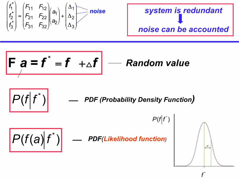
Random value

noise system is redundant

noise can be accounted

F a = f * = f +△f

PDF(Likelihood function)

P(f f * ) PDF (Probability Density Function)

P(f (a) f * )

P(f f * )

f*

P(a a(f * ))

a(f * )

P(f f * )

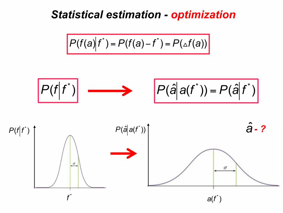
P(a a(f * )) = P(a f * )

Statistical estimation - optimization

P(f (a) f * ) = P(f (a)− f * ) = P(△f (a))

a - ?

sufficient – no more information can be obtained from f* consistent: unbiased: optimal – has highest formation from f*1,...,f*N effective – has highest possible formation from f*1,...,f*N jointly effective: – simultaneously have highest possible formation from f*1,...,f*N

€

f1*

f2*

f3*

"

#

$ $ $ $

%

&

' ' ' '

=

F11 F12

F21 F22

F31 F32

"

#

$ $ $

%

&

' ' '

a1

a2

"

# $

%

& ' +

Δ1

Δ2

Δ3

"

#

$ $ $

%

&

' ' '

noise

N= 3,4, … limited N= ∞

Properties of : a

a N→∞⎯ →⎯⎯ atrue

a

N= atrue

a1,a2,...,ak

sufficient – no more information can be obtained from f* (Darmois theorem: ~possible only for exponential PDF, i.e. N=∞) consistent: unbiased: optimal – has highest formation from f*1,...,f*N effective – has highest possible formation from f*1,...,f*N jointly effective: – simultaneously have highest possible formation from f*1,...,f*N

€

f1*

f2*

f3*

"

#

$ $ $ $

%

&

' ' ' '

=

F11 F12

F21 F22

F31 F32

"

#

$ $ $

%

&

' ' '

a1

a2

"

# $

%

& ' +

Δ1

Δ2

Δ3

"

#

$ $ $

%

&

' ' '

noise

N= 3,4, … limited N= ∞

N è∞, asymptotic

Properties of : a

a N→∞⎯ →⎯⎯ atrue

a

N= atrue

a1,a2,...,ak

Something to do with ?

Information Quantity: - ???

Information Quantity:

P(a f * )

P(a a(f * ))

a(f * )

The narower P(a) around atrue the better

P(atrue = ʹa )−P(a) The smaller the better

lnP(a) = lnP( ʹa )+ ∂lnP

∂a a= ʹa

(a− ʹa )+ 12∂2lnP∂a2

a= ʹa

(a− ʹa )2 + ...(a− ʹa )3 + ...

lnP(a)− lnP( ʹa ) = ∂lnP

∂a a= ʹa

(a− ʹa )+ 12∂2lnP∂a2

a= ʹa

(a− ʹa )2 + ...(a− ʹa )3 + ...

0

Taylor expansion in vicinity of atrue

The narrowest P(a)

lnP(a) ≈ lnP( ʹa )+ 1

2∂2lnP∂a2

a= ʹa

(a− ʹa )2

P(a) ∼ e12∂2 lnP∂a2

⎛

⎝⎜⎜

⎞

⎠⎟⎟(a− ʹa )2

⎛

⎝⎜⎜

⎞

⎠⎟⎟= e

−12

(a− ʹa )2

σ a2

= e

−12

(a− ʹa )2

−∂2 lnP∂a2

−1

−∂2lnP∂a2

⎛

⎝⎜

⎞

⎠⎟P da = −

∂lnP∂a

⎛

⎝⎜

⎞

⎠⎟

2

P da =∫ 1σ a

2∫

Fisher Information

σ a

2= −

∂2 lnP∂a2

−1

Smallest possible

2. Shannon Information:

Fisher Information:


1.

h P a( )( ) = −∂ 2lnP a f( )

∂ a2

⎛

⎝

⎜⎜

⎞

⎠

⎟⎟∫ P a f( )df

h P a( )( ) = −log2 P a f( )( )∫ P a f( )df →Nbits

Nbits- number of bits (binary digits) needed to represent the number of distinct estimates that could have be obtained

Gauss Probability Function

P(C

)

<C>

<ΔC2>1/2

€

Nsymbols ~ 2Nbits


2. Shannon Information:

Fisher Information:


1.

h P a( )( ) = −∂ 2lnP a f( )

∂ a2

⎛

⎝

⎜⎜

⎞

⎠

⎟⎟∫ P a f( )df = 1

Δa2

min

h P a( )( ) = −log2 P a f( )( )∫ P a f( )df =Nbits = f (−log2(σ ))

Nbits- number of bits (binary digits) needed to represent the number of distinct estimates that could have be obtained

Gauss Probability Function

P(C

)

<C>

<ΔC2>1/2

€

Nsymbols ~ 2Nbits


P a( ) = 1

2πσ 2e−

12

(a− ʹa )2

σ 2

∂lnP(a)∂a a= ʹa

= 0

lnP(a)− lnP( ʹa ) = ∂lnP

∂a a= ʹa

(a− ʹa )+ 12∂2lnP∂a2

a= ʹa

(a− ʹa )2 + ...(a− ʹa )3 + ...

0

MML (Method of Maximum Likelihood)

P(a

MML) ∼ e

−12

(a− ʹa )2

σ a2

= e

−12

(a− ʹa )2

−∂2 lnP∂a2

−1

σ a

2= Ia,Fisher( )−1

Smallest possible

∇ lnP(a)

a= 0 MML for several unknowns

P(a

MML) ∼ e

−12

(Δa)T Ca−1(Δa)

= e - 1

2 (Δa)T IFisher (Δa)

Fisher Information Matrix

IFisher{ }

ij= −

∂lnP a( )∂ai

∂lnP a( )∂aj

⎛

⎝⎜⎜

⎞

⎠⎟⎟∫ P a f( )df

Statistical Optimization

Cramer-Rao inequalityg - a characteristic linearly dependent on a

i.e. g = g1a1 + g2a2+… = g Ta, g - a vector of coefficients)

σ g

2 = g CagT ≥ g Ca,MMLg

T = g IFisher( )−1

gT

Smallest possible

aMML=(a1, a2,...)T – jointly effective !!!

Very important in practice

Optimality of MML:

aMML - asymptotically sufficient

aMML - asymptotically Normally distributed vector

aMML - asymptotically jointly effective (most accurate!)

aMML - asymptotically the best


Ca, MML = IFisher( )

−1

Optimality of LSM: for Δf is Normal: aLSM = aMML

if Δf is not Normal: - aLSM has the smallest variance among all unbiased linear estimators (Gauss-Markov theorem)-  aLSM asymptotically Normal

if P (...) Gaussian, MML = MLS


∇Ψ a( ) =∂Ψ a( )∂ai

= 0, (i =1,..,Na) Ψ a( ) = 1

2(f a( )− f∗)TC−1(f a( )− f∗) =min

⌢a = F1

TC1−1F1( )

−1F1

TC1−1f1

* Δf – Normal => Δa - Normal

LSM vs MML:

For Normal noise: aLSM = aMML For linear case: -  aLSM has smallest variance among unbiased estimators; -  aMML has smallest variance (asymptotically effective); -  both asymptotically Normal For non-linear case: -  aMML has smallest variance (asymptotically effective); -  both asymptotically Normal -  In practice aMML is often implemented as non-linear LSM,

i.e. aMML ≈ aLSM


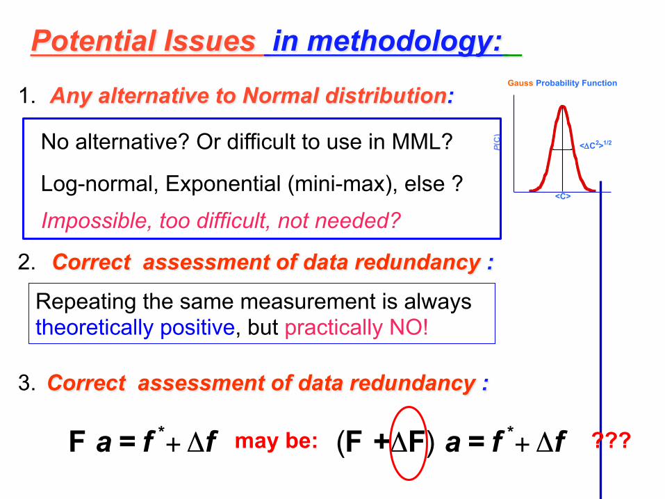
2. Correct assessment of data redundancy :

Any alternative to Normal distribution:

Potential Issues in methodology:

1. Gauss Probability Function

P (C

)

<C>

<ΔC2>1/2


No alternative? Or difficult to use in MML?

Log-normal, Exponential (mini-max), else ?

Impossible, too difficult, not needed?

Repeating the same measurement is always theoretically positive, but practically NO!

3. Correct assessment of data redundancy :

(F +ΔF) a = f *+ΔfF a = f *+Δf may be: ???

Non-negativity of solution

Convergence, Smoothness

f * =F a +Δf Normal

ai

p+1 = aip 1 + f j

* f jp − 1( ) !Fji( )

j=1

Nf

∏ ai

p+1= ai

p fi

∗fip"

#$$

%

&''

- Twomey-Chahine - Chahine

Δa = F1

TC1−1F1( )

−1F1

TC1−1△f1

* LSM

a - Can be negative

symmetric


(Dubovik and King 2000, Dubovik 2004)


f * =F a +Δf

ln(f * ) = ln(F a)+ lnΔf

Log - Normal

Normal

(for positively defined values e.g. Tarantola 1987)

Normal for additive errors Log-Normal for multiplicative errors



LSM in log Space

Newton Gauss Levenberg- Marquardt …


f * =F a +Δf


ap+1 = ap − DTC−1D( )

−1C−1DTΔ lnf p

Log - Normal

Normal

Normal △a ???



LSM in log Space

Newton Gauss Levenberg- Marquardt


f * =F a +Δf


lnap+1 = lnap − UTC−1U( )

−1C−1UTΔ lnf p

Log - Normal

Normal

△lnap Normal △aLog - Normal

P(f f * )

f*

P(a a(f * ))

a(f * )

P(f f * )

P(a a(f * )) = P(a f * )

Statistical estimation - optimization

P(f (a) f * ) = P(f (a)− f * ) = P(△f (a))

a - ?

Optimality of MML:

aMML - asymptotically sufficientaMML - asymptotically Normally distributed vectoraMML - asymptotically jointly effective (most accurate!)


f* = f a( ) +Δf

Conditions:

df a( )da

a

derivatives exist and limited in whole range of variability

- physical function

a ∈ −∞;+∞⎤⎦ ⎡⎣ f ∈ −∞;+∞⎤⎦ ⎡⎣

Derivations are in Dubovik and King 2000


ln ⌢ap+1 = ln ⌢ap − tp UTC−1U+γp I( )

−1UTC−1Δ lnf p

Levenberg – Marquardt ~ Newton - Gauss

∞

ln ⌢ap+1 = ln ⌢ap − tpUTC−1Δ lnf p

Steepest decent

ai

p+1 = aip 1 + f j

* f jp − 1( ) !Fji( )

j=1

Nf

∏ ai

p+1= ai

p fi

∗fip"

#$$

%

&''

- Twomey-Chahine - Chahine

Potential issue: Optimality of MML:aMML - asymptotically jointly effective (most accurate!)


Ca, MML = IFisher( )

−1 Smallest possible

What if: too large? or ?

det IFisher( )→ 0

Ca, MML

Additional constraints are needed!

~ exp −12Δf1

TΔf1σ 2

!

"##

$

%&& =max

2. Multi-Source Data:

1. One set of input data:

LSM for multiple data sets: P (...) - Probability Density Function (Likelihood)

P

P1,2,3=P1P2P3…~ exp −

12σ1

2

σ12

σ i2Δfi

TΔfi( )i∑

"

#$$

%

&'' =max

σ12

σ i2Δfi

TΔfi( )i∑ =min

where ∆i = fi*- fi(a) and fi

*- measurements or a priori data


ΔfiTΔfi( )σ12

=min

f1* =F1 a+Δ1

f2* =F2 a+Δ2...

"

#$$

%$$

Independent !!!

€

⌢ a = F1TC1

−1F1 +F2TC2

−1F2 + ...( )−1F1

TC1−1f1

* +F2TC2

−1f2* + ...( )

sensor 1 sensor 2

f1• = f * =F a +Δf

f2• = a* = a +Δa

f3• = 0 * = Sa +Δ(Δa)

"

#$$

%$$

sensor

a priori

⌢a = FTCf

−1F+Ca−1 + γSTS( )

−1FTCf

−1f * +Ca−1a*( )

Multi-Term LSM Multi-sensor data

Single-sensor data

Generalization of “Optimum estimation” and Phillips-Tikhonov-Twomey formulas

(e.g. see Dubovik 2004)

Inverse Problem: Retrieval of particle size distribution

from light scattering 0.01

0.02

0.04

0.05

0.07

0.1 1 10

dV/d

lnR

(µm

3 /µm

2 )

Radius (µm)

?

P(λ;Θ) = K λ;Θ;n,k,..( )dV r( )

drrmin

rmax

∫ dr

Fa = f *

2) How to solve ???

1). how to define ???

CONTENT 1. Atmospheric remote sensing as an inverse problem Primary linear problems; Essentially non-linear problems

2. Solving system of equations Matrix inversion solutions; linear iterative solutions; Solutions of non-linear systems Methods of constrained inversions - basic concept of overcoming solution instability 3. Statistical estimation concept Solving system of equation in the presence of noise in the data; Method of Maximum Likelihood

4. Least Squares Method

5. Methods of constrained inversions (for ill posed problems) Constrained inversions: Phillips–Tikhonov–Twomey , Kalman filter, Optimum estimations by Rogers, Bayesian statistics approach, etc 6. Including additional a priori information and Multi-Term Least Squares Method 7. Optimized solution of non-linear system of equations: Gauss–Newton and Quasi-Newton iterations, Levenberg–Marquardt iterations, Steepest-decent, etc. 8. Limitations of “statistical estimation”: A priori constraints on solution non-negativity, Accounting for effect of “redundant observations” 9. General recommendations, remote sensing applications, the GRASP algorithm 10. Introduction to assimilation and inverse modeling

“METHODS OF NUMERICAL INVERSION IN ATMOSPHERIC REMOTE SENSING AND INVERSE

MODELING: AN INTRODUCTION”

€

f1* = F1 a + Δ1

f2* = F2 a + Δ2

...

#

$ % %

& % %

Independent !!!

€

⌢ a = F1TC1

−1F1 +F2TC2

−1F2 + ...( )−1F1

TC1−1f1

* +F2TC2

−1f2* + ...( )

sensor 1 sensor 2

f * =F a +Δf

a* = a +Δa

"#$

%$

sensor

a priori

€

⌢ a = FTCf−1F + Ca

−1( )−1

FTCf−1f * + Ca

−1 a*( )


Single-sensor data

“Optimum Estimations” by Rodgers, Levenberg-Marquardt Maximum Entropy Method, Kalman Filter …, 4D Variational Assimilation (4DVR), … Assimilataion


Multi-Term LSM

smoothness

⌢a = FTCf−1F+Ca

−1( )−1FTCf

−1f * +Ca−1 a*( )

However:

f1• = f * =F a+Δff2• = 0 * = Sa +Δ(Δa)

"#$

%$

sensor

⌢a = FTCf−1F+STC0*

−1S( )−1FTCf

−1f *( )

Ca−1 = STC0*

−1S and a* = 0 *

det(STC0*−1S) = 0 Ca = ???

Identity ???

Optimal estimations

A priori smoothness constraints

f1* =F1 a+Δ1

f2* =F2 a+Δ2...

"

#$$

%$$

Independent !!!

€

⌢ a = F1TC1

−1F1 +F2TC2

−1F2 + ...( )−1F1

TC1−1f1

* +F2TC2

−1f2* + ...( )

sensor 1 sensor 2

f1• = f * =F a +Δf

f2• = a* = a +Δa

f3• = 0 * = Sa +Δ(Δa)

"

#$$

%$$

sensor

a priori

⌢a = FTCf−1F+Ca

−1 +STC0*−1S( )

−1FTCf

−1f * +Ca−1a*( )


Single-sensor data

Generalization of “Optimum estimation” and Phillips-Tikhonov-Twomey formulas


Non-linear inversion

Levenberg – Marquardt Ψ(a)

a - solution

a0 – initial guess

⌢ap+1 = ⌢ap − tp FTC−1F+γp I( )

−1FTC−1Δ lnf p

⌢ap+1 = ⌢ap − FTC−1F( )−1FTC−1Δ lnf p Δ

⌢ap - incorrect

Newton - Gauss

Independent !!!

Δ⌢a = F1

TC1−1F1 +F2

TC2−1F2 + ...( )

−1F1

TC1−1Δf1

* +F2TC2

−1Δf2* + ...( )

Δf1p =Fp Δap +Δ1

mes +Δ1linearizaion ap( )

0* = Δap +Δa*

"#$

%$

sensor

a priori

Multi-Term LSM

Levenberg-Marquardt

(e.g. see Dubovik 2004) f1 a( ) - nonlinear

Δ⌢ap = FTCf

−1F+Ca∗−1( )

−1FTCf

−1Δf * Δ⌢ap = ⌢ap −

⌢ap+1

⌢ap+1 = ⌢ap − FTF+γp I( )−1FTΔf p

γ p =εlineraization2

εa2

⎛

⎝⎜⎜

⎞

⎠⎟⎟ p→∞⎯ →⎯⎯ 0

ε lineraization

2 ~ Δf p( )TΔf p( ) − residual

Ca∗= I ε2

IDEAS + Cal/Val Workshop, Lille, France, April 6-7, 2017

analysis of numerical inverse algorithms · analysis of numerical inverse algorithms in atmosphere...

Documents