Geoderma Regional 2–3 (2014) 32–40

Contents lists available at ScienceDirect

Geoderma Regional

j ourna l homepage: www.e lsev ie r .com/ locate /geodrs

Analysing soil organic C gradients in a smallholder farming village ofEast Zimbabwe

D.F. van Apeldoorn a,b,⁎, B. Kempen c, H.M. Bartholomeus d, L. Rusinamhodzi a, S. Zingore e, M.P.W. Sonneveld b,1,K. Kok b, K.E. Giller a

a Plant Production Systems, Wageningen University, PO Box 430, 6700 AK Wageningen, The Netherlandsb Soil Geography and Landscape, Wageningen University, PO Box 47, 6700 AA Wageningen, The Netherlandsc ISRIC-World Soil Information, PO Box 353, 6700 AJ Wageningen, The Netherlandsd Laboratory of Geo-information Science and Remote Sensing, Wageningen University, PO Box 47, 6700 AA, Wageningen, The Netherlandse International Plant Nutrition Institute, Africa, C/O IFDC, East and Southern Africa Division ICIPE Compound, Duduville, Kasarani, Thika Road, Box 30772-00100, Nairobi, Kenya

⁎ Corresponding author at: PO Box 47, 6700 AAWagenE-mail addresses: Dirk.vanApeldoorn@wur.nl (D.F. van

Bas.Kempen@wur.nl (B. Kempen), Harm.Bartholomeus@wLeonard.Rusinamhodzi@gmail.com (L. Rusinamhodzi), SZKasper.Kok@wur.nl (K. Kok), Ken.Giller@wur.nl (K.E. Gille

1 Deceased.

http://dx.doi.org/10.1016/j.geodrs.2014.09.0062352-0094/© 2014 Elsevier B.V. All rights reserved.

a b s t r a c t

a r t i c l e i n f o

Article history:Received 1 July 2014Received in revised form 22 September 2014Accepted 22 September 2014Available online 26 September 2014

Keywords:Soil organic carbonDigital soil mappingZimbabweSoil textureLixisolsLuvisolsScale mismatch

We set out tomap the soil organic carbon (SOC) content, as an indicator of soil fertility, at the village scale, and torelate the SOC content to farm scalemanagement and landscape scale characteristics. Topsoil sampleswere takenat 100 random locations in theMurewa smallholder farming area in Zimbabwe and analysed for organic carbon.Using digital soilmapping techniques and Landsat TM imageswe could explain 50% of the observed SOC variance.The average SOC content was estimated to be 1.5%, although the sandy cropping area had a much lower averageof 0.8% and the red clays and valleys had higher average of 1.8%. The SOC variability could not be linked to farmmanagement. No fertility gradients were observed, mostly due to a strong dominance of clay content on the spa-tial distribution of SOC. Clay content was able to explain 57% of the SOC variance, while farm area and labour size,typically used for farmer typology, were able to explain only an additional minor part of the SOC variance. Thisstrong landscape scale effect needs to be included in future village-scale studies. We conclude that digital soilmapping of soil fertility gradients at the village scale has several scale issues that need to be addressed if theenvisioned global digital soil map is to be relevant for smallholder farmers in sub-Saharan Africa.

© 2014 Elsevier B.V. All rights reserved.

1. Introduction

Food production in sub-Saharan Africa does not keep pacewith pop-ulation growth (Ray et al., 2013; Tittonell and Giller, 2013). Poor soil fer-tility is the primary bio-physical constraint that results in poor yields(Sanchez, 2010). Next to the inherent variability of soils and their fertil-ity, management decisions result in the development of strong fertilitygradients (Giller et al., 2006, 2011; Masvaya et al., 2010; Tittonellet al., 2013, 2007a,b; Zingore et al., 2007b). These gradients are spatialpatterns of soil fertility, resulting from inherent differences in parentmaterial, position in the landscape and, above all, the preferentialallocation of manure, compost, mineral fertilizers and labour on fieldsnear the homesteads (Giller et al., 2011; Tittonell et al., 2013). As a re-sult, soil fertility declines with increasing distance from the homestead.These gradients are considered a key entry point for increasing resourceuse efficiency of scarce fertilizers and thereby increasing food security in

ingen, The Netherlands.Apeldoorn),ur.nl (H.M. Bartholomeus),

ingore@ipni.net (S. Zingore),r).

sub-Saharan Africa (Giller et al., 2011; Tittonell et al., 2013; Van Wijket al., 2009).

In the infertile, ancient soils that dominate much of sub-SaharanAfrica, soil organic carbon (SOC) is a key indicator of soil fertility. SOChas been identified as an essential natural resource in many land-based agro-ecosystems. It is considered the most important indicatorof soil quality and agronomic sustainability, because of its impact onother physical, chemical and biological soil properties (Reeves, 1997).In Zimbabwean smallholder systems, SOC content is highly correlatedwith soil physical properties (Dunjana et al., 2012), macro and micro-nutrients (Zingore et al., 2008) and ultimately maize yield(Rusinamhodzi et al., 2013). The accumulation of SOC is limited by theamount of C the field receives as unharvested biomass and manure. Inturn, the amount of biomass and manure produced in low-external-input systems is dependent on the soil fertility and regulated by theSOC content.

Differences in soil fertility betweenfields on similar soils are inducedby the strategic use of limited resources. Therefore, differences betweenfarms in resource endowments, and hence in access to nutrient re-sources, lead to different gradients (Masvaya et al., 2010). Zingoreet al. (2007a) showed that better-endowed farmers with ample accesstomanure, fertilizer andmeans of transportingmanure have only slightfertility gradients, while farmers with a limited amount of manure or

33D.F. van Apeldoorn et al. / Geoderma Regional 2–3 (2014) 32–40

labour, preferentially allocate such resources to the fields and gardensaround their homesteads, resulting in a strong decreasing gradient ofSOC. Farmers with no access to manure, or with a limited available la-bour force and a small cropping area, have no gradientwith only deplet-ed fields, as a result of prolonged cultivation with small applications offertilizer and no organic nutrient resources.

Soil fertility gradients have a strong influence on resource use effi-ciency for crop production: the returns to investment in fertilizer and la-bour are substantially reduced in depleted soils (Giller et al., 2006;Zingore et al., 2009). Village level explorations of soil fertility and organ-ic resources have been made (Rufino et al., 2011; Rusinamhodzi, 2013;Zingore et al., 2011), which revealed that crop–livestock integration atvillage level results in the concentration of nutrients on farms withlarge herds of cattle. The small areas of high fertility soils close to thehomesteads of wealthy farmers contributed the largest proportion ofthe total village maize yield, despite their fields occupying less thanhalf the area of the depleted fields (Zingore et al., 2011). These studiesassumed the same distributions of inherent soil characteristic betweenthe farmer resource groups, and did not analyse the spatial distributionof soil characteristics across the landscape. As soil fertility plays a crucialrole in food production at village level, there is a need to understand thespatial distribution of these fertility zones.

Recent advancements in digital soil mapping and modelling whichincorporate remote sensing products and geographic information tech-nologies have led to a vision of a high-resolution global digital soil map(Minasny et al., 2013; Sanchez et al., 2009). Thismap aims to be relevantto smallholder farming systems by providing them detailed soil infor-mation. Soil information can be used for developing site-specific nutri-ent management recommendations under highly variable soil fertilityconditions. Remotely sensed data in combination with digital soil map-ping techniques might be able to upscale the current mainly plot basedresearch on fertility gradients to larger areas. Moreover the availablehistoric imagery could provide insight in the emergence and dynamicsof these gradients by using available historic imagery.

As explained above, there is strong empirical and theoreticalevidence that soil fertility gradients play a self-reinforcing role indetermining the efficiency of response to inputs in smallholder farmingsystems of sub-Saharan Africa. Thus differences in farm resource en-dowment, soil type and number of years under cultivation lead to dis-tinct gradients of SOC at the farm scale. We hypothesize that thesegradients can be observed by remotely sensed data at the village scaleand can be related to landscape and management characteristics.

We tested this hypothesis in two steps. Our first objective was tomap SOC contents at the village scale using remote sensing imageryand digital soil mapping techniques. Secondly, we aimed to relate thepredicted SOC content to farm-scale management and to inherentlandscape-scale characteristics.

2. Materials and methods

2.1. Case study area

The study was conducted in the Murewa smallholder farming area,Zimbabwe (population density 104 people km−2) located about80 km east of Harare (17°49′S, 31°34′E). The area has a sub-tropical cli-mate and has relatively high potential for crop production. Murewa re-ceives 750 to 1000 mm of rainfall annually between November andApril. The soils are predominantly granitic sandy soils (Lixisols) withlow inherent fertility. A smaller proportion of the area has more fertilered, dolerite-derived clay soils (Luvisols) that are considered the bestagricultural soils in Zimbabwe (Nyamapfene, 1991). Farmers practiceamixed crop–livestock systemdominated bymaize (Zeamays L.). Cattleare themain livestock. In day time they are herded during the croppingseason but they graze freely on communal rangelands in the dry season.Cattle are kept in kraals close to homesteads at night. Close interactionsbetween crop and cattle production occur through crop residues that

are used to feed cattle andmanure is used to fertilize crops, particularlyat the fields closest to the homesteads. Only 6% of the households ownaround 10 heads of cattle, while 35% own less than 10 heads. Some33% of households own no cattle and have less than 1 ha of land. The re-maining 26% of the households do not own cattle and hold less than 2 haof land (Rusinamhodzi, 2013). The village has been intensively studiedand fertility gradients at farms have been reported (Rufino et al.,2011; Rusinamhodzi, 2013; Tittonell et al., 2007b; Zingore et al., 2007a).

2.2. Remote sensing data

To determine the spatial distribution of SOC, Landsat Thematic Map-per (TM) satellite imageswere used. Three georeferenced datasetsweredownloaded from the USGS data portal. The images were acquired on 5September 2008 and 11 and 27 November 2009. The downloaded im-ages were processed by NASA to the L1T level, indicating that theimage has the highest level of geodetic accuracy that can be achieved.Of these images the image DN values (an 8 bit value reflecting the radi-ation of the earth surface) were extracted by bilinear interpolation andused for further analysis. In addition, an ASTER digital elevation model(DEM) was downloaded from the same source.

2.3. Soil sampling

To investigate the spatial distribution of SOC, a stratified randomsampling method (De Gruijter et al., 2006) was applied. We have cho-sen for a design-based sampling method for two reasons. First, the sta-tistical model used in this study assumes that model residuals areindependent, which is guaranteed with a design-based sample (Brusand De Gruijter, 1997). Second, a probability sample allows us to obtainunbiased estimates of the mean soil property values and map accuracymeasures for the strata and for the sampling area. A stratification ofthe area was chosen to control sample allocation. We have chosen tosample stratum three more densely than the other strata since in stra-tum three most of the cropping takes place and we expected a largervariance in the cropping area than in the areaswith non-managed soils.

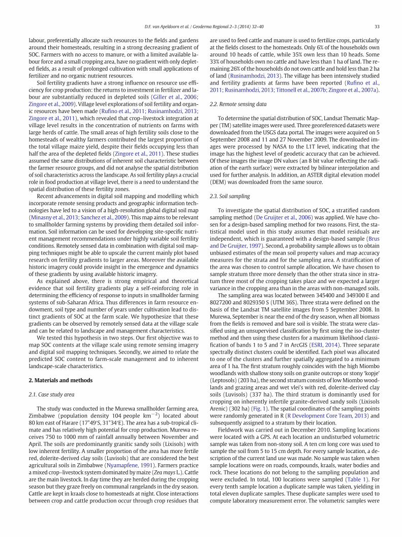
The sampling area was located between 345400 and 349300 E and8027200 and 8029350 S (UTM 36S). Three strata were defined on thebasis of the Landsat TM satellite images from 5 September 2008. InMurewa, September is near the end of the dry season, when all biomassfrom the fields is removed and bare soil is visible. The strata were clas-sified using an unsupervised classification by first using the iso-clustermethod and then using these clusters for a maximum likelihood classi-fication of bands 1 to 5 and 7 in ArcGIS (ESRI, 2014). Three separatespectrally distinct clusters could be identified. Each pixel was allocatedto one of the clusters and further spatially aggregated to a minimumarea of 1 ha. The first stratum roughly coincides with the high Miombowoodlands with shallow stony soils on granite outcrops or stony ‘kopje’(Leptosols) (203 ha), the second stratumconsists of lowMiombowood-lands and grazing areas and wet vlei's with red, dolerite-derived claysoils (Luvisols) (337 ha). The third stratum is dominantly used forcropping on inherently infertile granite-derived sandy soils (LixisolsArenic) (302 ha) (Fig. 1). The spatial coordinates of the sampling pointswere randomly generated in R (R Development Core Team, 2013) andsubsequently assigned to a stratum by their location.

Fieldwork was carried out in December 2010. Sampling locationswere located with a GPS. At each location an undisturbed volumetricsample was taken from non-stony soil. A ten cm long core was used tosample the soil from 5 to 15 cm depth. For every sample location, a de-scription of the current land use was made. No sample was taken whensample locations were on roads, compounds, kraals, water bodies androck. These locations do not belong to the sampling population andwere excluded. In total, 100 locations were sampled (Table 1). Forevery tenth sample location a duplicate sample was taken, yielding intotal eleven duplicate samples. These duplicate samples were used tocompute laboratory measurement error. The volumetric samples were

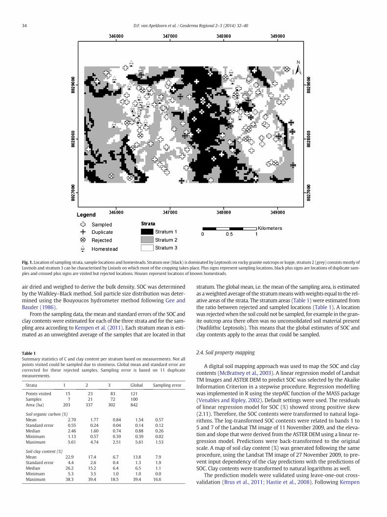
Fig. 1. Location of sampling strata, sample locations and homesteads. Stratumone (black) is dominated by Leptosols on rocky granite outcrops or kopje, stratum2 (grey) consistsmostly ofLuvisols and stratum 3 can be characterised by Lixisols onwhichmost of the cropping takes place. Plus signs represent sampling locations, black plus signs are locations of duplicate sam-ples and crossed plus signs are visited but rejected locations. Houses represent locations of known homesteads.

34 D.F. van Apeldoorn et al. / Geoderma Regional 2–3 (2014) 32–40

air dried and weighed to derive the bulk density. SOC was determinedby theWalkley–Black method. Soil particle size distribution was deter-mined using the Bouyoucos hydrometer method following Gee andBauder (1986).

From the sampling data, themean and standard errors of the SOC andclay contents were estimated for each of the three strata and for the sam-pling area according to Kempen et al. (2011). Each stratummean is esti-mated as an unweighted average of the samples that are located in that

Table 1Summary statistics of C and clay content per stratum based on measurements. Not allpoints visited could be sampled due to stoniness. Global mean and standard error arecorrected for these rejected samples. Sampling error is based on 11 duplicatemeasurements.

Strata 1 2 3 Global Sampling error

Points visited 15 23 83 121Samples 7 21 72 100Area (ha) 203 337 302 842

Soil organic carbon (%)Mean 2.70 1.77 0.84 1.54 0.57Standard error 0.55 0.24 0.04 0.14 0.12Median 2.46 1.60 0.74 0.88 0.26Minimum 1.13 0.57 0.39 0.39 0.02Maximum 5.61 4.74 2.51 5.61 1.53

Soil clay content (%)Mean 22.9 17.4 6.7 13.8 7.9Standard error 4.4 2.6 0.4 1.3 1.9Median 26.2 15.2 6.4 6.5 1.1Minimum 5.3 3.5 1.0 1.0 0.0Maximum 38.3 39.4 18.5 39.4 16.6

stratum. The global mean, i.e. themean of the sampling area, is estimatedas aweighted average of the stratummeanswithweights equal to the rel-ative areas of the strata. The stratum areas (Table 1) were estimated fromthe ratio between rejected and sampled locations (Table 1). A locationwas rejectedwhen the soil could not be sampled, for example in the gran-ite outcrop area there often was no unconsolidated soil material present(Nudilithic Leptosols). This means that the global estimates of SOC andclay contents apply to the areas that could be sampled.

2.4. Soil property mapping

A digital soil mapping approach was used to map the SOC and claycontents (McBratney et al., 2003). A linear regression model of LandsatTM Images and ASTER DEM to predict SOC was selected by the AkaikeInformation Criterion in a stepwise procedure. Regression modellingwas implemented in R using the stepAIC function of the MASS package(Venables and Ripley, 2002). Default settings were used. The residualsof linear regression model for SOC (%) showed strong positive skew(2.11). Therefore, the SOC contents were transformed to natural loga-rithms. The log-transformed SOC contents were related to bands 1 to5 and 7 of the Landsat TM image of 11 November 2009, and the eleva-tion and slope that were derived from the ASTER DEM using a linear re-gression model. Predictions were back-transformed to the originalscale. A map of soil clay content (%) was generated following the sameprocedure, using the Landsat TM image of 27 November 2009, to pre-vent input dependency of the clay predictions with the predictions ofSOC. Clay contents were transformed to natural logarithms as well.

The prediction models were validated using leave-one-out cross-validation (Brus et al., 2011; Hastie et al., 2008). Following Kempen

35D.F. van Apeldoorn et al. / Geoderma Regional 2–3 (2014) 32–40

et al. (2011) and De Gruijter et al. (2006), the mean error (ME), meanabsolute error (MAE) and root mean squared error (RMSE) were esti-mated. Estimates of these parameters are based on the predictionerror. The prediction error is calculated as the difference between thepredicted and observed values at a validation location. In addition, theroot median square error (RMedSE) is estimated. For skewed distribu-tions of squared errors, the median square error and its square root isa more robust statistic than the ‘average’ error.

2.5. Landscape management and SOC interactions

A separate dataset of farm characteristics (Rusinamhodzi et al., 2013)was used to allocate management to the soil property maps. The datasetcontains information on land ownership (area and time), area under cul-tivation, household size and available labour force and cattle ownership.Following Zingore et al. (2007a), farm resource groups (RG) were firstseparated on cattle ownershipwithRG1havingmore than 9heads of cat-tle (in total 3 farms), and RG 2 having 1 to 7 heads of cattle (16 farms).Farms with no cattle were separated into two groups based on theirarea, with farms with 1 ha or more belong to RG 3 (13 farms) and thosewith less than 1 ha belong to RG 4 (14 farms). Of the 80 householdsinterviewed, 46 could be assigned to a geo-referenced location (Fig. 2).The household dataset was made spatially explicit via the location ofthe homestead and high-resolution imagery of Google Earth. Since someof the households were located outside the area where soil sampleswere taken, the SOC and clay contents were predicted for the whole vil-lage from Landsat TM images and DEM (Fig. 2). The farms in Murewamostly consist of one large field demarcated into smaller plots with onlyfew farmers having detached plots far from homestead (Zingore et al.,

Fig. 2.Predicted soil organic carbon (SOC) content (%). Thepoints represent the locations of knowindicates farms owningmore than 8 heads of cattle, RG 2 indicates farms owning 1 to 7 heads offarms with less than 1 ha and no cattle. The white dashed line indicates the sample area.

2007a). With the use of Google Earth images, these adjacent fields couldbe assigned to a homestead (Fig. 2). By combining the SOC and claymaps with the resource groups, interactions between management andlandscape could be investigated.

To investigate the fertility gradients per resource group, firstly allpixels inside the farmers' fields were assigned to their resource groups.Subsequently these pixels were ranked regarding to their distance fromthe homestead. With intervals of 30 m the average SOC was calculated.These averages were then plotted as a transect going from the home-stead to the outfields for each resource group.

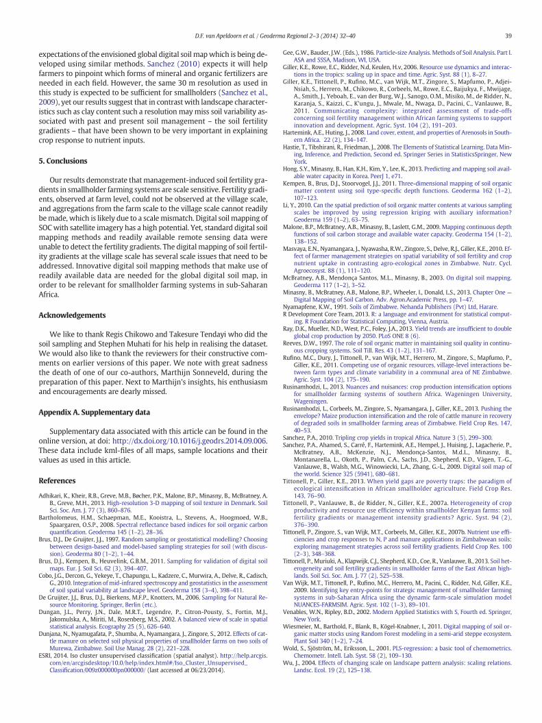
To further investigate themanagement–landscape interactions, par-tial least square regression (PLSR) was used (Wold et al., 2001). PLSRfinds a linear regressionmodel by projecting themanagement and land-scape variables and the SOC into a new space. PLSR is insensitive to co-linearity of the predictors, the vectors of these predictors will have thesame or opposite direction in the new projected space. PLSR explainsthe maximum variance of predicted SOC using all spatial and manage-ment data. In the partial least square regression nine variables wereused to explain predicted SOC content of pixels belonging to farmers'fields. The nine variables were distance, clay content, family size, laboursize, time of cultivation, land area cultivated, land area owned, selling ofown labour, and number of cattle.

3. Results

3.1. Village scale maps

In total we sampled 72 points in the third stratum and 21 points inthe second stratum and another 7 in the first stratum (Fig. 1, Table 1).

nhomesteads and solidblack lines demarcate their adjacentfields. Resource group (RG) 1cattle, RG 3 indicates farms owningmore than 1 ha of land but no cattle and RG 4 indicates

36 D.F. van Apeldoorn et al. / Geoderma Regional 2–3 (2014) 32–40

In total 100 locationswere analysed for SOC content and 99 for clay con-tent. The first stratum along 347500 Ewas difficult to sample due to therocky character of this area leading to a rejection of the majority of thesample locations.Most households are located on the sandy soils in stra-tum three. The average SOC content of the village area is estimated as1.53%; the average clay content is estimated as 14%. Estimates byZingore et al. (2011) for a neighbouring village (30 km to the east) arewell within the 95% confidence limit of our estimates.

Stepwise linear regression of the SOC content on the Landsat TMimage of 11November 2009 andDEMderivatives resulted in the follow-ing model:

SOC log%ð Þ ¼ 2:98−0:022� TM band 4−0:007� TM band 5: ð1Þ

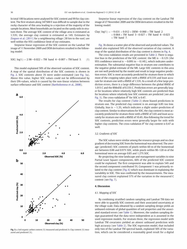
This model explained 50% of the observed variation of SOC content.A map of the spatial distribution of the SOC contents is shown inFig. 2. SOC contents above 3% were under-estimated (see Fig. 3a).Above this value, higher SOC values could not be differentiated bytheir DN-values, which is caused by the non-linear relation betweensurface reflectance and SOC content (Bartholomeus et al., 2008).

Fig. 3. a. Soil organic carbon content (%)measured and predicted. b. Clay content (%)mea-sured and predicted (%).

Stepwise linear regression of the clay content on the Landsat TMimage of 27November 2009 and theDEMderivatives resulted in the fol-lowing model:

Clay log%ð Þ ¼ −9:631þ 0:012� DEM−0:060� TM band 2þ 0:064� TM band 3−0:027� TM band 4−0:023� TM band 7: ð2Þ

Fig. 3b shows a scatter plot of the observed and predicted values. Themodel also explained 50% of the observed variation of clay content. Amap of the spatial distribution of the clay content is shown in Fig. 4.

The cross-validation results are presented in Table 2. There is nega-tive bias in the prediction of the SOC content: the ME is −0.12% (the95% confidence interval is −0.09% to−0.14%), which indicates under-estimation. The substantial negative bias in stratum one contributes tothe negative global estimate of the ME. Large SOC contents in this areaare not well predicted by themodel and result in large negative predic-tion errors. SOC is most accurately predicted for stratum three in whichmost of the cropping takes place with a RMSE of 0.33% and least accu-rate for stratum onewith a RMSE of 1.53%. As a result of a few large pre-diction errors, there is a large difference between the global RMSE of1.01% C and the RMedSE of 0.33% C. Prediction errors are generally larg-er for locations where relatively high SOC contents are predicted thanfor locations where relatively low SOC contents are predicted (see alsoFig. 3). The cross-validation R2 for SOC is 0.47.

The results for clay content (Table 2) show biased predictions instratum one. The predicted clay content is on average 6.8% too low.Globally, bias is −1.3%, which indicates a slight under-prediction ofclay content. Similar to observations for SOC, the clay content ismost ac-curately predicted for stratum threewith a RMSE of 3.6% and least accu-rately for stratum onewith a RMSE of 10.4%. Also following the trend forSOC contents, prediction errors were generally larger for soils withhigher clay contents. The cross-validation R2 for clay content is 0.47 aswell.

3.2. Gradients of SOC

The SOCvalueswere similar among the resource groups and no cleargradient of decreasing SOC from thehomesteadwas observed. The aver-age (predicted) SOC contents of pixels within 60 m of the homesteadare between 0.88 and 0.97% SOC, while pixels within 90–120 m of thehomestead were on average 0.85 and 1.27% SOC.

Re-projecting the nine landscape andmanagement variables to ninePartial Least Square components, 60% of the predicted SOC contentcould be explained. The first component was able to explain 54% andthe second component contributed 5%. Component 1 was primarily re-lated to the clay content (Fig. 6) which was dominant in explaining thevariability in SOC. This was confirmed by the measurements. The mea-sured clay content explained 57% of the variation in the measured Ccontent (see Fig. 7).

4. Discussion

4.1. Mapping of SOC

By combining stratified random sampling and Landsat TM data wewere able to quantify SOC contents and their associated uncertainty atthe village scale. Data obtained by a random sampling design yields anunbiased estimate of global quantities of soil properties and the associ-ated standard errors (see Table 1). Moreover, the random sampling de-sign guaranteed that the data were independent as is assumed in theused regression models. For stratum three, the regression model withLandsat TM covariates yielded an almost unbiased prediction withhigh accuracy (see Table 2). The SOC regression model, that includedonly two of the Landsat TM spectral bands, explained 50% of the varia-tion, which can be considered a reasonably good result for a digital

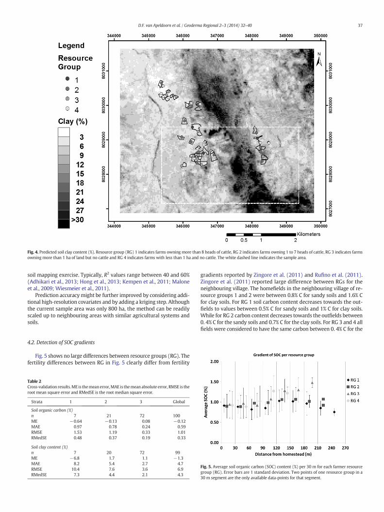
Fig. 4. Predicted soil clay content (%). Resource group (RG) 1 indicates farms owning more than 8 heads of cattle, RG 2 indicates farms owning 1 to 7 heads of cattle, RG 3 indicates farmsowning more than 1 ha of land but no cattle and RG 4 indicates farms with less than 1 ha and no cattle. The white dashed line indicates the sample area.

37D.F. van Apeldoorn et al. / Geoderma Regional 2–3 (2014) 32–40

soil mapping exercise. Typically, R2 values range between 40 and 60%(Adhikari et al., 2013; Hong et al., 2013; Kempen et al., 2011; Maloneet al., 2009; Wiesmeier et al., 2011).

Prediction accuracymight be further improved by considering addi-tional high-resolution covariates and by adding a kriging step. Althoughthe current sample area was only 800 ha, the method can be readilyscaled up to neighbouring areas with similar agricultural systems andsoils.

4.2. Detection of SOC gradients

Fig. 5 shows no large differences between resource groups (RG). Thefertility differences between RG in Fig. 5 clearly differ from fertility

Table 2Cross-validation results.ME is themean error,MAE is themean absolute error, RMSE is theroot mean square error and RMedSE is the root median square error.

Strata 1 2 3 Global

Soil organic carbon (%)n 7 21 72 100ME −0.64 −0.13 0.08 −0.12MAE 0.97 0.78 0.24 0.59RMSE 1.53 1.19 0.33 1.01RMedSE 0.48 0.37 0.19 0.33

Soil clay content (%)n 7 20 72 99ME −6.8 1.7 1.1 −1.3MAE 8.2 5.4 2.7 4.7RMSE 10.4 7.6 3.6 6.9RMedSE 7.3 4.4 2.1 4.3

gradients reported by Zingore et al. (2011) and Rufino et al. (2011).Zingore et al. (2011) reported large difference between RGs for theneighbouring village. The homefields in the neighbouring village of re-source groups 1 and 2 were between 0.8% C for sandy soils and 1.6% Cfor clay soils. For RG 1 soil carbon content decreases towards the out-fields to values between 0.5% C for sandy soils and 1% C for clay soils.While for RG 2 carbon content decreases towards the outfields between0. 4% C for the sandy soils and 0.7% C for the clay soils. For RG 3 and 4 allfields were considered to have the same carbon between 0. 4% C for the

Fig. 5. Average soil organic carbon (SOC) content (%) per 30 m for each farmer resourcegroup (RG). Error bars are 1 standard deviation. Two points of one resource group in a30 m segment are the only available data-points for that segment.

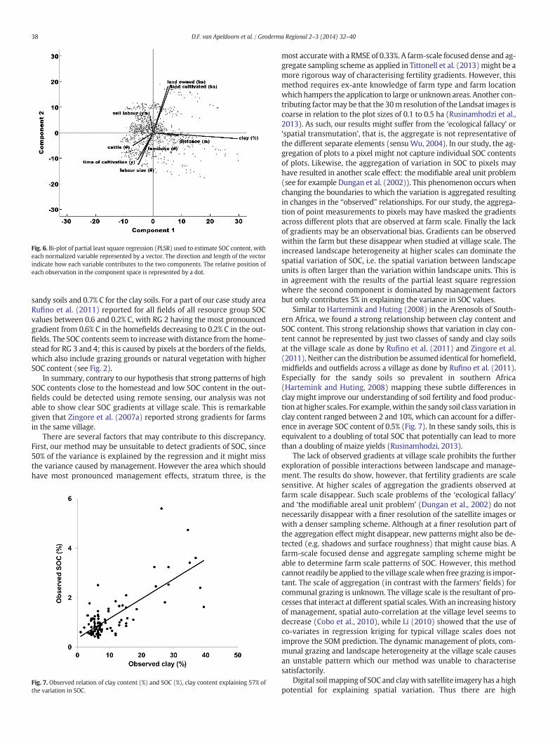
Fig. 6. Bi-plot of partial least square regression (PLSR) used to estimate SOC content, witheach normalized variable represented by a vector. The direction and length of the vectorindicate how each variable contributes to the two components. The relative position ofeach observation in the component space is represented by a dot.

38 D.F. van Apeldoorn et al. / Geoderma Regional 2–3 (2014) 32–40

sandy soils and 0.7% C for the clay soils. For a part of our case study areaRufino et al. (2011) reported for all fields of all resource group SOCvalues between 0.6 and 0.2% C, with RG 2 having the most pronouncedgradient from 0.6% C in the homefields decreasing to 0.2% C in the out-fields. The SOC contents seem to increase with distance from the home-stead for RG 3 and 4; this is caused by pixels at the borders of the fields,which also include grazing grounds or natural vegetation with higherSOC content (see Fig. 2).

In summary, contrary to our hypothesis that strong patterns of highSOC contents close to the homestead and low SOC content in the out-fields could be detected using remote sensing, our analysis was notable to show clear SOC gradients at village scale. This is remarkablegiven that Zingore et al. (2007a) reported strong gradients for farmsin the same village.

There are several factors that may contribute to this discrepancy.First, our method may be unsuitable to detect gradients of SOC, since50% of the variance is explained by the regression and it might missthe variance caused by management. However the area which shouldhave most pronounced management effects, stratum three, is the

Fig. 7. Observed relation of clay content (%) and SOC (%), clay content explaining 57% ofthe variation in SOC.

most accuratewith a RMSE of 0.33%. A farm-scale focused dense and ag-gregate sampling scheme as applied in Tittonell et al. (2013)might be amore rigorous way of characterising fertility gradients. However, thismethod requires ex-ante knowledge of farm type and farm locationwhich hampers the application to large or unknown areas. Another con-tributing factormay be that the 30m resolution of the Landsat images iscoarse in relation to the plot sizes of 0.1 to 0.5 ha (Rusinamhodzi et al.,2013). As such, our results might suffer from the ‘ecological fallacy’ or‘spatial transmutation’, that is, the aggregate is not representative ofthe different separate elements (sensu Wu, 2004). In our study, the ag-gregation of plots to a pixel might not capture individual SOC contentsof plots. Likewise, the aggregation of variation in SOC to pixels mayhave resulted in another scale effect: the modifiable areal unit problem(see for example Dungan et al. (2002)). This phenomenon occurs whenchanging the boundaries to which the variation is aggregated resultingin changes in the “observed” relationships. For our study, the aggrega-tion of point measurements to pixels may have masked the gradientsacross different plots that are observed at farm scale. Finally the lackof gradients may be an observational bias. Gradients can be observedwithin the farm but these disappear when studied at village scale. Theincreased landscape heterogeneity at higher scales can dominate thespatial variation of SOC, i.e. the spatial variation between landscapeunits is often larger than the variation within landscape units. This isin agreement with the results of the partial least square regressionwhere the second component is dominated by management factorsbut only contributes 5% in explaining the variance in SOC values.

Similar to Hartemink and Huting (2008) in the Arenosols of South-ern Africa, we found a strong relationship between clay content andSOC content. This strong relationship shows that variation in clay con-tent cannot be represented by just two classes of sandy and clay soilsat the village scale as done by Rufino et al. (2011) and Zingore et al.(2011). Neither can the distribution be assumed identical for homefield,midfields and outfields across a village as done by Rufino et al. (2011).Especially for the sandy soils so prevalent in southern Africa(Hartemink and Huting, 2008) mapping these subtle differences inclay might improve our understanding of soil fertility and food produc-tion at higher scales. For example,within the sandy soil class variation inclay content ranged between 2 and 10%, which can account for a differ-ence in average SOC content of 0.5% (Fig. 7). In these sandy soils, this isequivalent to a doubling of total SOC that potentially can lead to morethan a doubling of maize yields (Rusinamhodzi, 2013).

The lack of observed gradients at village scale prohibits the furtherexploration of possible interactions between landscape and manage-ment. The results do show, however, that fertility gradients are scalesensitive. At higher scales of aggregation the gradients observed atfarm scale disappear. Such scale problems of the ‘ecological fallacy’and ‘the modifiable areal unit problem’ (Dungan et al., 2002) do notnecessarily disappear with a finer resolution of the satellite images orwith a denser sampling scheme. Although at a finer resolution part ofthe aggregation effect might disappear, new patterns might also be de-tected (e.g. shadows and surface roughness) that might cause bias. Afarm-scale focused dense and aggregate sampling scheme might beable to determine farm scale patterns of SOC. However, this methodcannot readily be applied to the village scalewhen free grazing is impor-tant. The scale of aggregation (in contrast with the farmers' fields) forcommunal grazing is unknown. The village scale is the resultant of pro-cesses that interact at different spatial scales.With an increasing historyof management, spatial auto-correlation at the village level seems todecrease (Cobo et al., 2010), while Li (2010) showed that the use ofco-variates in regression kriging for typical village scales does notimprove the SOM prediction. The dynamic management of plots, com-munal grazing and landscape heterogeneity at the village scale causesan unstable pattern which our method was unable to characterisesatisfactorily.

Digital soilmapping of SOC and claywith satellite imagery has a highpotential for explaining spatial variation. Thus there are high

39D.F. van Apeldoorn et al. / Geoderma Regional 2–3 (2014) 32–40

expectations of the envisioned global digital soil mapwhich is being de-veloped using similar methods. Sanchez (2010) expects it will helpfarmers to pinpoint which forms of mineral and organic fertilizers areneeded in each field. However, the same 30 m resolution as used inthis study is expected to be sufficient for smallholders (Sanchez et al.,2009), yet our results suggest that in contrast with landscape character-istics such as clay content such a resolution maymiss soil variability as-sociated with past and present soil management – the soil fertilitygradients – that have been shown to be very important in explainingcrop response to nutrient inputs.

5. Conclusions

Our results demonstrate thatmanagement-induced soil fertility gra-dients in smallholder farming systems are scale sensitive. Fertility gradi-ents, observed at farm level, could not be observed at the village scale,and aggregations from the farm scale to the village scale cannot readilybemade, which is likely due to a scalemismatch. Digital soil mapping ofSOCwith satellite imagery has a high potential. Yet, standard digital soilmapping methods and readily available remote sensing data wereunable to detect the fertility gradients. The digital mapping of soil fertil-ity gradients at the village scale has several scale issues that need to beaddressed. Innovative digital soil mapping methods that make use ofreadily available data are needed for the global digital soil map, inorder to be relevant for smallholder farming systems in sub-SaharanAfrica.

Acknowledgements

We like to thank Regis Chikowo and Takesure Tendayi who did thesoil sampling and Stephen Muhati for his help in realising the dataset.We would also like to thank the reviewers for their constructive com-ments on earlier versions of this paper. We note with great sadnessthe death of one of our co-authors, Marthijn Sonneveld, during thepreparation of this paper. Next to Marthijn's insights, his enthusiasmand encouragements are dearly missed.

Appendix A. Supplementary data

Supplementary data associated with this article can be found in theonline version, at doi: http://dx.doi.org/10.1016/j.geodrs.2014.09.006.These data include kml-files of all maps, sample locations and theirvalues as used in this article.

References

Adhikari, K., Kheir, R.B., Greve, M.B., Bøcher, P.K., Malone, B.P., Minasny, B., McBratney, A.B., Greve, M.H., 2013. High-resolution 3-D mapping of soil texture in Denmark. SoilSci. Soc. Am. J. 77 (3), 860–876.

Bartholomeus, H.M., Schaepman, M.E., Kooistra, L., Stevens, A., Hoogmoed, W.B.,Spaargaren, O.S.P., 2008. Spectral reflectance based indices for soil organic carbonquantification. Geoderma 145 (1–2), 28–36.

Brus, D.J., De Gruijter, J.J., 1997. Random sampling or geostatistical modelling? Choosingbetween design-based and model-based sampling strategies for soil (with discus-sion). Geoderma 80 (1–2), 1–44.

Brus, D.J., Kempen, B., Heuvelink, G.B.M., 2011. Sampling for validation of digital soilmaps. Eur. J. Soil Sci. 62 (3), 394–407.

Cobo, J.G., Dercon, G., Yekeye, T., Chapungu, L., Kadzere, C., Murwira, A., Delve, R., Cadisch,G., 2010. Integration ofmid-infrared spectroscopy and geostatistics in the assessmentof soil spatial variability at landscape level. Geoderma 158 (3–4), 398–411.

De Gruijter, J.J., Brus, D.J., Bierkens, M.F.P., Knotters, M., 2006. Sampling for Natural Re-source Monitoring. Springer, Berlin (etc.).

Dungan, J.L., Perry, J.N., Dale, M.R.T., Legendre, P., Citron-Pousty, S., Fortin, M.J.,Jakomulska, A., Miriti, M., Rosenberg, M.S., 2002. A balanced view of scale in spatialstatistical analysis. Ecography 25 (5), 626–640.

Dunjana, N., Nyamugafata, P., Shumba, A., Nyamangara, J., Zingore, S., 2012. Effects of cat-tle manure on selected soil physical properties of smallholder farms on two soils ofMurewa, Zimbabwe. Soil Use Manag. 28 (2), 221–228.

ESRI, 2014. Iso cluster unsupervised classification (spatial analyst). http://help.arcgis.com/en/arcgisdesktop/10.0/help/index.html#/Iso_Cluster_Unsupervised_Classification/009z000000pn000000/ (last accessed at 06/23/2014).

Gee, G.W., Bauder, J.W. (Eds.), 1986. Particle-size Analysis. Methods of Soil Analysis. Part I.ASA and SSSA, Madison, WI, USA.

Giller, K.E., Rowe, E.C., Ridder, N.d, Keulen, H.v, 2006. Resource use dynamics and interac-tions in the tropics: scaling up in space and time. Agric. Syst. 88 (1), 8–27.

Giller, K.E., Tittonell, P., Rufino, M.C., van Wijk, M.T., Zingore, S., Mapfumo, P., Adjei-Nsiah, S., Herrero, M., Chikowo, R., Corbeels, M., Rowe, E.C., Baijukya, F., Mwijage,A., Smith, J., Yeboah, E., van der Burg, W.J., Sanogo, O.M., Misiko, M., de Ridder, N.,Karanja, S., Kaizzi, C., K'ungu, J., Mwale, M., Nwaga, D., Pacini, C., Vanlauwe, B.,2011. Communicating complexity: integrated assessment of trade-offsconcerning soil fertility management within African farming systems to supportinnovation and development. Agric. Syst. 104 (2), 191–203.

Hartemink, A.E., Huting, J., 2008. Land cover, extent, and properties of Arenosols in South-ern Africa. 22 (2), 134–147.

Hastie, T., Tibshirani, R., Friedman, J., 2008. The Elements of Statistical Learning. Data Min-ing, Inference, and Prediction, Second ed. Springer Series in StatisticsSpringer, NewYork.

Hong, S.Y., Minasny, B., Han, K.H., Kim, Y., Lee, K., 2013. Predicting and mapping soil avail-able water capacity in Korea. PeerJ 1, e71.

Kempen, B., Brus, D.J., Stoorvogel, J.J., 2011. Three-dimensional mapping of soil organicmatter content using soil type-specific depth functions. Geoderma 162 (1–2),107–123.

Li, Y., 2010. Can the spatial prediction of soil organic matter contents at various samplingscales be improved by using regression kriging with auxiliary information?Geoderma 159 (1–2), 63–75.

Malone, B.P., McBratney, A.B., Minasny, B., Laslett, G.M., 2009. Mapping continuous depthfunctions of soil carbon storage and available water capacity. Geoderma 154 (1–2),138–152.

Masvaya, E.N., Nyamangara, J., Nyawasha, R.W., Zingore, S., Delve, R.J., Giller, K.E., 2010. Ef-fect of farmer management strategies on spatial variability of soil fertility and cropnutrient uptake in contrasting agro-ecological zones in Zimbabwe. Nutr. Cycl.Agroecosyst. 88 (1), 111–120.

McBratney, A.B., Mendonça Santos, M.L., Minasny, B., 2003. On digital soil mapping.Geoderma 117 (1–2), 3–52.

Minasny, B., McBratney, A.B., Malone, B.P., Wheeler, I., Donald, L.S., 2013. Chapter One —

Digital Mapping of Soil Carbon. Adv. Agron.Academic Press, pp. 1–47.Nyamapfene, K.W., 1991. Soils of Zimbabwe. Nehanda Publishers (Pvt) Ltd, Harare.R Development Core Team, 2013. R: a language and environment for statistical comput-

ing. R Foundation for Statistical Computing, Vienna, Austria.Ray, D.K., Mueller, N.D., West, P.C., Foley, J.A., 2013. Yield trends are insufficient to double

global crop production by 2050. PLoS ONE 8 (6).Reeves, D.W., 1997. The role of soil organic matter in maintaining soil quality in continu-

ous cropping systems. Soil Till. Res. 43 (1–2), 131–167.Rufino, M.C., Dury, J., Tittonell, P., van Wijk, M.T., Herrero, M., Zingore, S., Mapfumo, P.,

Giller, K.E., 2011. Competing use of organic resources, village-level interactions be-tween farm types and climate variability in a communal area of NE Zimbabwe.Agric. Syst. 104 (2), 175–190.

Rusinamhodzi, L., 2013. Nuances and nuisances: crop production intensification optionsfor smallholder farming systems of southern Africa. Wageningen University,Wageningen.

Rusinamhodzi, L., Corbeels, M., Zingore, S., Nyamangara, J., Giller, K.E., 2013. Pushing theenvelope? Maize production intensification and the role of cattle manure in recoveryof degraded soils in smallholder farming areas of Zimbabwe. Field Crop Res. 147,40–53.

Sanchez, P.A., 2010. Tripling crop yields in tropical Africa. Nature 3 (5), 299–300.Sanchez, P.A., Ahamed, S., Carré, F., Hartemink, A.E., Hempel, J., Huising, J., Lagacherie, P.,

McBratney, A.B., McKenzie, N.J., Mendonça-Santos, M.d.L., Minasny, B.,Montanarella, L., Okoth, P., Palm, C.A., Sachs, J.D., Shepherd, K.D., Vågen, T.-G.,Vanlauwe, B., Walsh, M.G., Winowiecki, L.A., Zhang, G.-L., 2009. Digital soil map ofthe world. Science 325 (5941), 680–681.

Tittonell, P., Giller, K.E., 2013. When yield gaps are poverty traps: the paradigm ofecological intensification in African smallholder agriculture. Field Crop Res.143, 76–90.

Tittonell, P., Vanlauwe, B., de Ridder, N., Giller, K.E., 2007a. Heterogeneity of cropproductivity and resource use efficiency within smallholder Kenyan farms: soilfertility gradients or management intensity gradients? Agric. Syst. 94 (2),376–390.

Tittonell, P., Zingore, S., van Wijk, M.T., Corbeels, M., Giller, K.E., 2007b. Nutrient use effi-ciencies and crop responses to N, P and manure applications in Zimbabwean soils:exploring management strategies across soil fertility gradients. Field Crop Res. 100(2–3), 348–368.

Tittonell, P., Muriuki, A., Klapwijk, C.J., Shepherd, K.D., Coe, R., Vanlauwe, B., 2013. Soil het-erogeneity and soil fertility gradients in smallholder farms of the East African high-lands. Soil Sci. Soc. Am. J. 77 (2), 525–538.

Van Wijk, M.T., Tittonell, P., Rufino, M.C., Herrero, M., Pacini, C., Ridder, N.d, Giller, K.E.,2009. Identifying key entry-points for strategic management of smallholder farmingsystems in sub-Saharan Africa using the dynamic farm-scale simulation modelNUANCES-FARMSIM. Agric. Syst. 102 (1–3), 89–101.

Venables, W.N., Ripley, B.D., 2002. Modern Applied Statistics with S, Fourth ed. Springer,New York.

Wiesmeier, M., Barthold, F., Blank, B., Kögel-Knabner, I., 2011. Digital mapping of soil or-ganic matter stocks using Random Forest modeling in a semi-arid steppe ecosystem.Plant Soil 340 (1–2), 7–24.

Wold, S., Sjöström, M., Eriksson, L., 2001. PLS-regression: a basic tool of chemometrics.Chemometr. Intell. Lab. Syst. 58 (2), 109–130.

Wu, J., 2004. Effects of changing scale on landscape pattern analysis: scaling relations.Landsc. Ecol. 19 (2), 125–138.

40 D.F. van Apeldoorn et al. / Geoderma Regional 2–3 (2014) 32–40

Zingore, S., Murwira, H.K., Delve, R.J., Giller, K.E., 2007a. Influence of nutrient managementstrategies on variability of soil fertility, crop yields and nutrient balances on small-holder farms in Zimbabwe. Agric. Ecosyst. Environ. 119 (1–2), 112–126.

Zingore, S., Murwira, H.K., Delve, R.J., Giller, K.E., 2007b. Soil type, management historyand current resource allocation: three dimensions regulating variability in crop pro-ductivity on African smallholder farms. Field Crop Res. 101 (3), 296–305.

Zingore, S., Delve, R.J., Nyamangara, J., Giller, K.E., 2008. Multiple benefits of manure: thekey to maintenance of soil fertility and restoration of depleted sandy soils on Africansmallholder farms. Nutr. Cycl. Agroecosyst. 80 (3), 267–282.

Zingore, S., González-Estrada, E., Delve, R.J., Herrero, M., Dimes, J.P., Giller, K.E., 2009. Anintegrated evaluation of strategies for enhancing productivity and profitability ofresource-constrained smallholder farms in Zimbabwe. Agric. Syst. 101 (1–2), 57–68.

Zingore, S., Tittonell, P., Corbeels, M., van Wijk, M.T., Giller, K.E., 2011. Managing soilfertility diversity to enhance resource use efficiencies in smallholder farmingsystems: a case from Murewa District, Zimbabwe. Nutr. Cycl. Agroecosyst. 90(1), 87–103.