an undergraduate introduction to financial mathematics
DESCRIPTION
The book proposes an introduction to financial mathematics focused on undergraduate students.TRANSCRIPT
n U n d e r g r a d u a t e
I n t r o d u c t i o n t o
M a t h e m a t i c s
J Robert Buchanan
A n U n d e r g r a d u a t e
{f^ I n t r o d u c t i o n t o
F i n a n c i a l ^ ! M a t h e m a t i c s

This page is intentionally left blank
•M'!'M>»M4
J Robert Buchanan MiNersviile University, USA
World Scientific NEW JERSEY • LONDON - SINGAPORE • BEIJING • SHANGHAI • HONG KONG • TAIPEI • CHENNAI
Published by
World Scientific Publishing Co. Pte. Ltd.
5 Toh Tuck Link, Singapore 596224
USA office: 27 Warren Street, Suite 401-402, Hackensack, NJ 07601
UK office: 57 Shelton Street, Covent Garden, London WC2H 9HE
British Library Cataloguing-in-Publication Data A catalogue record for this book is available from the British Library.
AN UNDERGRADUATE INTRODUCTION TO FINANCIAL MATHEMATICS
Copyright © 2006 by World Scientific Publishing Co. Pte. Ltd.
All rights reserved. This book, or parts thereof, may not be reproduced in any form or by any means, electronic or mechanical, including photocopying, recording or any information storage and retrieval system now known or to be invented, without written permission from the Publisher.
For photocopying of material in this volume, please pay a copying fee through the Copyright Clearance Center, Inc., 222 Rosewood Drive, Danvers, MA 01923, USA. In this case permission to photocopy is not required from the publisher.
ISBN 981-256-637-6
Printed in Singapore by World Scientific Printers (S) Pte Ltd

Dedication
For my wife, Monika.

This page is intentionally left blank
Preface
This book is intended for an audience with an undergraduate level of exposure to calculus through elementary multivariable calculus. The book assumes no background on the part of the reader in probability or statistics. One of my objectives in writing this book was to create a readable, reasonably self-contained introduction to financial mathematics for people wanting to learn some of the basics of option pricing and hedging. My desire to write such a book grew out of the need to find an accessible book for undergraduate mathematics majors on the topic of financial mathematics. I have taught such a course now three times and this book grew out of my lecture notes and reading for the course. New titles in financial mathematics appear constantly, so in the time it took me to compose this book there may have appeared several superior works on the subject. Knowing the amount of work required to produce this book, I stand in awe of authors such as those.
This book consists of ten chapters which are intended to be read in order, though the well-prepared reader may be able to skip the first several with no loss of understanding in what comes later. The first chapter is on interest and its role in finance. Both discretely compounded and continuously compounded interest are treated there. The book begins with the theory of interest because this topic is unlikely to scare off any reader no matter how long it has been since they have done any formal mathematics.
The second and third chapters provide an introduction to the concepts of probability and statistics which will be used throughout the remainder of the book. Chapter Two deals with discrete random variables and emphasizes the use of the binomial random variable. Chapter Three introduces continuous random variables and emphasizes the similarities and differences between discrete and continuous random variables. The nor-
vii
viii An Undergraduate Introduction to Financial Mathematics
mal random variable and the close related lognormal random variable are introduced and explored in the latter chapter.
In the fourth chapter the concept of arbitrage is introduced. For readers already well versed in calculus, probability, and statistics, this is the first material which may be unfamiliar to them. The assumption that financial calculations are carried out in an "arbitrage free" setting pervades the remainder of the book. The lack of arbitrage opportunities in financial transactions ensures that it is not possible to make a risk free profit. This chapter includes a discussion of the result from linear algebra and operations research known as the Duality Theorem of Linear Programming.
The fifth chapter introduces the reader to the concepts of random walks and Brownian motion. The random walk underlies the mathematical model of the value of securities such as stocks and other financial instruments whose values are derived from securities. The choice of material to present and the method of presentation is difficult in this chapter due to the complexities and subtleties of stochastic processes. I have attempted to introduce stochastic processes in an intuitive manner and by connecting elementary stochastic models of some processes to their corresponding deterministic counterparts. Ito's Lemma is introduced and an elementary proof of this result is given based on the multivariable form of Taylor's Theorem. Readers whose interest is piqued by material in Chapter Five should consult the bibliography for references to more comprehensive and detailed discussions of stochastic calculus.
Chapter Six introduces the topic of options. Both European and American style options are discussed though the emphasis is on European options. Properties of options such as the Put/Call Parity formula are presented and justified. In this chapter we also derive the partial differential equation and boundary conditions used to price European call and put options. This derivation makes use of the earlier material on arbitrage, stochastic processes and the Put/Call Parity formula.
The seventh chapter develops the solution to the Black-Scholes PDE. There are several different methods commonly used to derive the solution to the PDE and students benefit from different aspects of each derivation. The method I choose to solve the PDE involves the use of the Fourier Transform. Thus this chapter begins with a brief discussion of the Fourier and Inverse Fourier Transforms and their properties. Most three- or four-semester elementary calculus courses include at least an optional section on the Fourier Transform, thus students will have the calculus background necessary to follow this discussion. It also provides exposure to the Fourier
Preface IX
Transform for students who will be later taking a course in PDEs and more importantly exposure for students who will not take such a course. After completing this derivation of the Black-Scholes option pricing formula students should also seek out other derivations in the literature for the purposes of comparison.
Chapter Eight introduces some of the commonly discussed partial derivatives of the Black-Scholes option pricing formula. These partial derivatives help the reader to understand the sensitivity of option prices to movements in the underlying security's value, the risk-free interest rate, and the volatility of the underlying security's value. The collection of partial derivatives introduced in this chapter is commonly referred to as "the Greeks" by many financial practitioners. The Greeks are used in the ninth chapter on hedging strategies for portfolios. Hedging strategies are used to protect the value of a portfolio against movements in the underlying security's value, the risk-free interest rate, and the volatility of the underlying security's value. Mathematically the hedging strategies remove some of the low order terms from the Black-Scholes option pricing formula making it less sensitive to changes in the variables upon which it depends. Chapter Nine will discuss and illustrate several examples of hedging strategies.
Chapter Ten extends the ideas introduced in Chapter Nine by modeling the effects of correlated movements in the values of investments. The tenth chapter discusses several different notions of optimality in selecting portfolios of investments. Some of the classical models of portfolio selection are introduced in this chapter including the Capital Assets Pricing Model (CAPM) and the Minimum Variance Portfolio.
It is the author's hope that students will find this book a useful introduction to financial mathematics and a springboard to further study in this area. Writing this book has been hard, but intellectually rewarding work.
During the summer of 2005 a draft version of this manuscript was used by the author to teach a course in financial mathematics. The author is indebted to the students of that class for finding numerous typographical errors in that earlier version which were corrected before the camera ready copy was sent to the publisher. The author wishes to thank Jill Bachstadt, Jason Buck, Mark Elicker, Kelly Flynn, Jennifer Gomulka, Nicole Hundley, Alicia Kasif, Stephen Kluth, Patrick McDevitt, Jessica Paxton, Christopher Rachor, Timothy Ren, Pamela Wentz, Joshua Wise, and Michael Zrncic.
A list of errata and other information related to this book can be found at a web site I created:

x An Undergraduate Introduction to Financial Mathematics
http://banach.millersville.edu/~bob/book/
Please feel free to share your comments, criticism, and (I hope) praise for this work through the email address that can be found at that site.
J. Robert Buchanan Lancaster, PA, USA
October 31, 2005
Contents
Preface vii
1. The Theory of Interest 1
1.1 Simple Interest 1 1.2 Compound Interest 3 1.3 Continuously Compounded Interest 4 1.4 Present Value 5 1.5 Rate of Return 11 1.6 Exercises 12
2. Discrete Probability 15
2.1 Events and Probabilities 15 2.2 Addition Rule 17 2.3 Conditional Probability and Multiplication Rule 18 2.4 Random Variables and Probability Distributions 21 2.5 Binomial Random Variables 23 2.6 Expected Value 24 2.7 Variance and Standard Deviation 29 2.8 Exercises 32
3. Normal Random Variables and Probability 35
3.1 Continuous Random Variables 35 3.2 Expected Value of Continuous Random Variables 38 3.3 Variance and Standard Deviation 40 3.4 Normal Random Variables 42 3.5 Central Limit Theorem 49
xi
X l l An Undergraduate Introduction to Financial Mathematics
3.6 Lognormal Random Variables 51 3.7 Properties of Expected Value 55 3.8 Properties of Variance 58 3.9 Exercises 61
4. The Arbitrage Theorem 63
4.1 The Concept of Arbitrage 63 4.2 Duality Theorem of Linear Programming 64
4.2.1 Dual Problems 66 4.3 The Fundamental Theorem of Finance 72 4.4 Exercises 74
5. Random Walks and Brownian Motion 77
5.1 Intuitive Idea of a Random Walk 77 5.2 First Step Analysis 78 5.3 Intuitive Idea of a Stochastic Process 91 5.4 Stock Market Example 95 5.5 More About Stochastic Processes 97 5.6 Ito's Lemma 98 5.7 Exercises 101
6. Options 103
6.1 Properties of Options 104 6.2 Pricing an Option Using a Binary Model 107 6.3 Black-Scholes Partial Differential Equation 110 6.4 Boundary and Initial Conditions 112 6.5 Exercises 114
7. Solution of the Black-Scholes Equation 115
7.1 Fourier Transforms 115 7.2 Inverse Fourier Transforms 118 7.3 Changing Variables in the Black-Scholes PDE 119 7.4 Solving the Black-Scholes Equation 122 7.5 Exercises 127
8. Derivatives of Black-Scholes Option Prices 131
8.1 Theta 131 8.2 Delta 133
Contents xiii
8.3 Gamma 135 8.4 Vega 136 8.5 Rho 138 8.6 Relationships Between A, 9 , and T 139 8.7 Exercises 141
9. Hedging 143
9.1 General Principles 143 9.2 Delta Hedging 145 9.3 Delta Neutral Portfolios 149 9.4 Gamma Neutral Portfolios 151 9.5 Exercises 153
10. Optimizing Portfolios 155
10.1 Covariance and Correlation 155 10.2 Optimal Portfolios 164 10.3 Utility Functions 165 10.4 Expected Utility 171 10.5 Portfolio Selection 173 10.6 Minimum Variance Analysis 177 10.7 Mean Variance Analysis 186 10.8 Exercises 191
Appendix A Sample Stock Market Data 195
Appendix B Solutions to Chapter Exercises 203
B.l The Theory of Interest 203 B.2 Discrete Probability 206 B.3 Normal Random Variables and Probability 212 B.4 The Arbitrage Theorem 225 B.5 Random Walks and Brownian Motion 231 B.6 Options 235 B.7 Solution of the Black-Scholes Equation 239 B.8 Derivatives of Black-Scholes Option Prices 245 B.9 Hedging 249 B.10 Optimizing Portfolios 255
Bibliography 265
Index 267
Chapter 1
The Theory of Interest
One of the first types of investments that people learn about is some variation on the savings account. In exchange for the temporary use of an investor's money, a bank or other financial institution agrees to pay interest, a percentage of the amount invested, to the investor. There are many different schemes for paying interest. In this chapter we will describe some of the most common types of interest and contrast their differences. Along the way the reader will have the opportunity to renew their acquaintanceship with exponential functions and the geometric series. Since an amount of capital can be invested and earn interest and thus numerically increase in value in the future, the concept of present value will be introduced. Present value provides a way of comparing values of investments made at different times in the past, present, and future. As an application of present value, several examples of saving for retirement and calculation of mortgages will be presented. Sometimes investments pay the investor varying amounts of money which change over time. The concept of rate of return can be used to convert these payments in effective interest rates, making comparison of investments easier.
1.1 Simple Interest
In exchange for the use of a depositor's money, banks pay a fraction of the account balance back to the depositor. This fractional payment is known as interest. The money a bank uses to pay interest is generated by investments and loans that the bank makes with the depositor's money. Interest is paid in many cases at specified times of the year, but nearly always the fraction of the deposited amount used to calculate the interest is called the interest rate and is expressed as a percentage paid per year.
1
2 An Undergraduate Introduction to Financial Mathematics
For example a credit union may pay 6% annually on savings accounts. This means that if a savings account contains $100 now, then exactly one year from now the bank will pay the depositor $6 (which is 6% of $100) provided the depositor maintains an account balance of $100 for the entire year.
In this chapter and those that follow, interest rates will be denoted symbolically by r. To simplify the formulas and mathematical calculations, when r is used it will be converted to decimal form even though it may still be referred to as a percentage. The 6% annual interest rate mentioned above would be treated mathematically as r — 0.06 per year. The initially deposited amount which earns the interest will be called the principal amount and will be denoted P. The sum of the principal amount and any earned interest will be called the compound amount and A will represent it symbolically. Therefore the relationship between P, r, and A for a single year period is
A = P + Pr = P(l + r).
The interest, once paid to the depositor, is the depositor's to keep. Banks and other financial institutions "pay" the depositor by adding the interest to the depositor's account. Unless the depositor withdraws the interest or some part of the principal, the process begins again for another interest period. Thus two interest periods (think of them as years) after the initial deposit the compound amount would be
A = P(l + r) + P ( l + r)r = P{1 + r)2.
Continuing in this way we can see that t years after the initial deposit of an amount P , the compound amount A will grow to
A = P{l + r)t (1.1)
This is known as the simple interest formula. A mathematical "purist" may wish to establish Eq. (1.1) using the principle of induction.
Banks and other interest-paying financial institutions often pay interest more than a single time per year. The simple interest formula must be modified to track the compound amount for interest periods of other than one year.
The Theory of Interest 3
1.2 Compound Interest
The typical interest bearing savings or checking account will be described an investor as earning a specific annual interest rate compounded monthly. In this section will be compare and contrast compound interest to the simple interest case of the previous section. Whenever interest is allowed to earn interest itself, an investment is said to earn compound interest. In this situation, part of the interest is paid to the depositor more than once per year. Once paid, the interest begins earning interest. We will let the number of compounding periods per year be n. For example for interest "compounded monthly" n = 12. Only two small modifications to the simple interest formula (1.1) are needed to calculate the compound interest. First, it is now necessary to think of the interest rate per compounding period. If the annual interest rate is r, then the interest rate per compounding period is r/n. Second, the elapsed time should be thought of as some number of compounding periods rather than years. Thus with n compounding periods per year, the number of compounding periods in t years is nt. Therefore the formula for compound interest is
A = P(l+r-)a'. (1.2)
Example 1.1 Suppose an account earns 5.75% annually compounded monthly. If the principal amount is $3104 then after three and one half years the compound amount will be
0 0575\ ( 1 2 ) ( 3-5 )
A = 3104(1 + H ^ I M =3794.15.
The reader should verify that if the principal in the previous example earned a simple interest rate of 5.75% then the compound amount after 3.5 years would be only $3774.88. Thus happily for the depositor, compound interest builds wealth faster than simple interest. Frequently it is useful to compare an annual interest rate with compounding to an equivalent simple interest, i.e. to the simple annual interest rate which would generate the sample amount of interest as the annual compound rate. This equivalent interest rate is called the effective interest rate. For the amounts and rates mentioned in the previous example we can find the effective interest
4 An Undergraduate Introduction to Financial Mathematics
rate by solving the equation
3104 (l+°-^y = 3104(1 + re)
1.05904 = 1 + re
0.05904 = re
Thus the annual interest rate of 5.75% compounded monthly is equivalent to an effective annual simple rate of 5.904%.
Intuitively it seems that more compounding periods per year implies a higher effective annual interest rate. In the next section we will explore the limiting case of frequent compounding going beyond semiannually, quarterly, monthly, weekly, daily, hourly, etc. to continuously.
1.3 Continuously Compounded Interest
Mathematically when considering the effect on the compound amount of more frequent compounding, we are contemplating a limiting process. In symbolic form we would like to find the compound amount A which satisfies the equation
/ r \ n t
A= lim P 1 + - • (1.3) n—>oo V n/
Fortunately there is a simple expression for the value of the limit on the right-hand side of Eq. (1.3). We will find it by working on the limit
lim f l + - ) " . n—too V 7J /
This limit is indeterminate of the form 1°°. We will evaluate it through a standard approach using the natural logarithm and l'HopitaPs Rule. The reader should consult an elementary calculus book such as [Smith and Minton (2002)] for more details. We see that if y = (1 + r/n)n, then
lny = m ( l + - )
= nln( l + r/n)
_ ln(l + r/n)
~ ljn
which is indeterminate of the form 0/0 as n —> oo. To apply l'Hopital's Rule we take the limit of the derivative of the numerator over the derivative of
The Theory of Interest 5
the denominator. Thus
lim In y = lim £(ln(l + r/n))
£ (Vn) r
= lim . . n^oo 1 + r/n
= r
Thus limn^oo y — er. Finally we arrive at the formula for continuously compounded interest,
A = Pert. (1.4)
This formula may seem familiar since it is often presented as the exponential growth formula in elementary algebra, precalculus, or calculus. The quantity A has the property that A changes with time t at a rate proportional to A itself.
Example 1.2 Suppose $3585 is deposited in an account which pays interest at an annual rate of 6.15% compounded continuously. After two and one half years the principal plus earned interest will have grown to
A = 3585e(0'0615)(2-5) = 4180.82.
The effective simple interest rate is the solution to the equation
e 0.0615 = 1 + r e
which implies re = 6.34305%.
1.4 Present Value
One of the themes we will see many times in the study of financial mathematics is the comparison of the value of a particular investment at the present time with the value of the investment at some point in the future. This is the comparison between the present value of an investment versus its future value. We will see in this section that present and future value play central roles in planning for retirement and determining loan payments. Later in this book present and future values will help us determine a fair price for stock market derivatives.
6 An Undergraduate Introduction to Financial Mathematics
The future value t years from now of an invested amount P subject to an annual interest rate r compounded continuously is
A = Pert.
Thus by comparison with Eq. (1.4), the future value of P is just the compound amount of P monetary units invested in a savings account earning interest r compounded continuously for t years. By contrast the present value of A in an environment of interest rate r compounded continuously for t years is
P = Ae~rt.
In other words if an investor wishes to have A monetary units in savings t years from now and they can place money in a savings account earning interest at an annual rate r compounded continuously, the investor should deposit P monetary units now. There are also formulas for future and present value when interest is compounded at discrete intervals, not continuously. If the interest rate is r annually with n compounding periods per year then the future value of P is
Compare this equation with Eq. (1.2). Simple algebra shows then the present value of P earning interest at rate r compounded n times per year for t years is
By choosing n = 1, the case of simple interest can be handled.
Example 1.3 Suppose an investor will receive payments at the end of the next six years in the amounts shown in the table.
Year
Payment
1 465
2 233
3 632
4 365
5 334
6 248
If the interest rate is 3.99% compounded monthly, what is the present value of the investments? Assuming the first payment will arrive one year from
The Theory of Interest 7
now, the present value is the sum
465 [ 1 + ^ V 1 2 + 2 3 3 fl + ^ V 2 4
+ 632 (l • 12 ; +233{1+^r) +M2[l+^2
+ 365(l + ^ )" \334( l + ^ ) " ° + 248(l + M f ) " 7 2
= 2003.01
Notice that the present value of the payments from the investment is different from the sum of the payments themselves (which is 2277).
Unless the reader is among the very fortunate few who can always pay cash for all purchases, you may some day apply for a loan from a bank or other financial institution. Loans are always made under the assumptions of a prevailing interest rate (with compounding), an amount to be borrowed, and the lifespan of the loan, i.e. the time the borrower has to repay the loan. Usually portions of the loan must be repaid at regular intervals (for example, monthly). Now we turn our attention to the question of using the amount borrowed, the length of the loan, and the interest rate to calculate the loan payment.
A very helpful mathematical tool for answering questions regarding present and future values is the geometric series. Suppose we wish to find the sum
S=l + a + a2 + --- + an (1.5)
where n is a positive whole number. If both sides of Eq. (1.5) are multiplied by a and then subtracted from Eq. (1.5) we have
S - aS = 1 + a + a2 + • • • + an - (a + a2 + a3 + • • • + an+1)
5(1 - o) = 1 - an+1
1 - an+1
S~ 1-a
provided a ^ l . Now we will apply this tool to the task of finding out the monthly
amount of a loan payment. Suppose someone borrows P to purchase a new car. The bank issuing the automobile loan charges interest at the annual rate of r compounded n times per year. The length of the loan will be t years. The monthly payment can be calculated if we apply the principle that the present value of all the payments made must equal the amount borrowed. Suppose the payment amount is the constant x. If the first
8 An Undergraduate Introduction to Financial Mathematics
payment must be made at the end of the first compounding period, then the present value of all the payments is
n
= x{i + r-r
i - a + = x —
x(l
l 1 -
1 -
- ) " n '
r \ 2 + - ) 2 + •• n
- ( 1 + S ) - 1
nt
• + x(l + - ) -n
-nt
Therefore the relationship between the interest rate, the compounding frequency, the length of the loan, the principal amount borrowed, and the payment amount is expressed in the following equation.
n x —
r 1+"-
n (1.6)
Example 1.4 If a person borrows $25000 for five years at an interest rate of 4.99% compounded monthly and makes equal monthly payments, the payment amount will be
x = 25000(0.0499/12) (l - [1 + (0.0499/12)]~(12)(5)) = 471.67.
Similar reasoning can be used when determining how much to save for retirement. Suppose a person is 25 years of age now and plans to retire at age 65. For the next 40 years they plan to invest a portion of their monthly income in securities which earn interest at the rate of 10% compounded monthly. After retirement the person plans on receiving a monthly payment (an annuity) in the absolute amount of $1500. The amount of money the person should invest monthly while working can be determined by equating the present value of all their deposits with the present value of all their withdrawals. The first deposit will be made one month from now and the first withdrawal will be made 481 months from now. The monthly deposit amount will be be denoted by the symbol x. The present value of all the deposits made into the retirement account is
fVii°- i (v x f i i ^ y 1 1 - ^ ^ " 4 8 0
hS v) y 12; i - ( i + ^ r « 117.765a;.
The Theory of Interest 9
Meanwhile the present value of all the annuity payments is
1500 Y^ 840 / 0.10V* A o.ioy481i-(i + ^ ) - 3 6 0
1 + = 1500 1 + , • — , . 12 J v 12 J l - fi + ^ ior
w 3182.94.
Thus x w 27.03 dollars per month. This seems like a small amount to invest, but such is the power of compound interest and starting a savings plan for retirement early. If the person waits ten years to begin saving for retirement, but all other factors remain the same then
K.^)-.^ 360
X
i=l 720 0 10 \
1500 Y^ ( l + " j y ) ~ 8616.36 i=361 ^ '
which implies the person must invest x ~ 75.61 monthly. Waiting ten years to begin saving for retirement nearly triples the amount which the future retiree must set aside for retirement.
The initial amounts invested are of course invested for a longer period of time and thus contribute a proportionately greater amount to the future value of the retirement account.
Example 1.5 Suppose two people will retire in twenty years. One begins saving immediately for retirement but due to unforeseen circumstances must abandon their savings plan after four years. The amount they put aside during those first four years remains invested, but no additional amounts are invested during the last sixteen years of their working life. The other person waits four years before putting any money into a retirement savings account. They save for retirement only during the last sixteen years of their working life. Let us explore the difference in the final amount of retirement savings that each person will possess. For the purpose of this example we will assume that the interest rate is r = 0.05 compounded monthly and that both workers will invest the same amount x, monthly. The first worker has upon retirement an account whose present value is
z f V l + ^5 , ^ ^ ^ ^ V 12
10 An Undergraduate Introduction to Financial Mathematics
The present value of the second worker's total investment is
^ / 0.05 V * x l ^ [ l + ~ w ) ~ 108.102a;.
Thus the second worker retires with a larger amount of retirement savings; however, the ratio of their retirement balances is only 43.423/108.102 « 0.40. The first worker saves approximately 40% of what the second worker saves in only one fifth of the time.
The discussion of retirement savings makes no provision for rising prices. The economic concept of inflation is the phenomenon of the decrease in the purchasing power of a unit of money relative to a unit amount of goods or services. The rate of inflation (usually expressed as an annual percentage rate, similar to an interest rate) varies with time and is a function of many factors including political, economic, and international factors. While the causes of inflation can be many and complex, inflation is generally described as a condition which results from an increase in the amount of money in circulation without a commensurate increase in the amount of available goods. Thus relative to the supply of goods, the value of the currency is decreased. This can happen when wages are arbitrarily increased without an equal increase in worker productivity.
We now focus on the effect that inflation may have on the worker planning to save for retirement. If the interest rate on savings is rs and the inflation rate is r^, the monthly amount put into savings by the worker must be discounted by an effective rate rs + r^. Then once the worker is retired the monthly annuity must be discounted by the rate rs — r^. Returning to the earlier example consider the case in which rs = 0.10, the worker will save for 40 years and live on a monthly annuity whose inflation adjusted value will be $1500 for 30 years, and the rate of inflation will be ri = 0.03 for the entire lifespan of the worker/retiree. Assuming the worker will make the first deposit in one month the present value of all deposits to be made is
v f i i °- i 3r . f n o-i3vii-(i+g#)"48° w 91.784a;.
The Theory of Interest 11
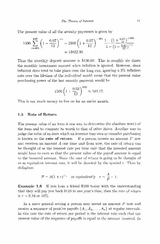
The present value of all the annuity payments is given by
^ f 0 .07 \ " 1 , / 0.07 V 4 8 1 1 - ( 1 + T ^ " 3 6 ° 1500 > 1 + = 1500 1 ' > v — 12
i=481 v 7 v 7 x I 1 ^ 12 J
« 13822.30.
Thus the monthly deposit amount is $150.60. This is roughly six times the monthly investment amount when inflation is ignored. However, since inflation does tend to take place over the long run, ignoring a 3% inflation rate over the lifetime of the individual would mean that the present value purchasing power of the last annuity payment would be
0.03^ 840
1500(1 + ——I « 184.17.
This is not much money to live on for an entire month.
1.5 Rate of Return
The present value of an item is one way to determine the absolute worth of the item and to compare its worth to that of other items. Another way to judge the value of an item which an investor may own or consider purchasing is known as the rate of return. If a person invests an amount P now and receives an amount A one time unit from now, the rate of return can be thought of as the interest rate per time unit that the invested amount would have to earn so that the present value of the payoff amount is equal to the invested amount. Since the rate of return is going to be thought of as as equivalent interest rate, it will be denoted by the symbol r. Then by definition
P = A(l + r ) _ 1 or equivalently r = — — 1.
Example 1.6 If you loan a friend $100 today with the understanding that they will pay you back $110 in one year's time, then the rate of return is r = 0.10 or 10%.
In a more general setting a person may invest an amount P now and receive a sequence of positive payoffs {Ai,A2,..., An} at regular intervals. In this case the rate of return per period is the interest rate such that the present value of the sequence of payoffs is equal to the amount invested. In

12 An Undergraduate Introduction to Financial Mathematics
this case n
i= i
It is not clear from this definition that r has a unique value for all choices of P and payoff sequences. Defining the function f(r) to be
n
f(r) = -P + J2Ml + r)-* (1.7) i= l
we can see that f(r) is continuous on the open interval (—1, oo). In the limit as r approaches —1 from the right, the function values approach positive infinity. On the other hand as r approaches positive infinity, the function values approach — P < 0 asymptotically. Thus by the Intermediate Value Theorem (p. 108 of [Smith and Minton (2002)]) there exists r* with - 1 < r* < oo such that f(r*) = 0. The reader is encouraged to show that r* is unique in the exercises.
Rates of return can be either positive or negative. If /(0) > 0, i.e., the sum of the payoffs is greater than the amount invested then r* > 0 since f(r) changes sign on the interval [0, oo). If the sum of the payoffs is less than the amount invested then /(0) < 0 and the rate of return in negative. In this case the function f(r) changes sign on the interval (—1,0].
Example 1.7 Suppose you loan a friend $100 with the agreement that they will pay you at the end of the next five years amounts {21, 22, 23, 24, 25}. The rate of return per year is the solution to the equation,
21 22 23 24 25 " 1 0 ° + TT7 + (1 + r)2 + (1 + r ) 3 + (1 + r ) 4 + (1 + r ) 5 " '
Newton's Method (Sec. 3.2 of [Smith and Minton (2002)]) can be used to approximate the solution r* K, 0.047.
1.6 Exercises
(1) Suppose that $3659 is deposited in a savings account which earns 6.5% simple interest. What is the compound amount after five years?
(2) Suppose that 3993 is deposited in an account which earns 4.3% interest. What is the compound amount after two years if the interest is compounded
The Theory of Interest 13
(a) monthly? (b) weekly? (c) daily? (d) continuously?
(3) Find the effective annual simple interest rate which is equivalent to 8% interest compounded quarterly.
(4) You are preparing to open a bank which will accept deposits into savings accounts and which will pay interest compounded monthly. In order to be competitive you must meet or exceed the interest paid by another bank which pays 5.25% compounded daily. What is the minimum interest rate you can pay and remain competitive?
(5) Suppose you have $1000 to deposit in one of two types of savings accounts. One account pays interest at an annual rate of 4.75% compounded daily, while the other pays interest at an annual rate of 4.75% compounded continuously. How long would it take for the compound amounts to differ by $1?
(6) Many textbooks determine the formula for continuously compounded interest through an argument which avoids the use of l'Hopital's Rule (for example [Goldstein et al. (1999)]). Beginning with Eq. (1.3) let h = r/n. Then
P ( l + - ) n ' = P ( l + / i ) ( 1 / h ) r t
and we can focus on finding the l i m ^ o ( l + h)1'11. Show that
( l + /j)l/k = e(l/h)ln(l + h)
and take the limit of both sides as h —> 0. Hint: you can use the definition of the derivative in the exponent on the right-hand side.
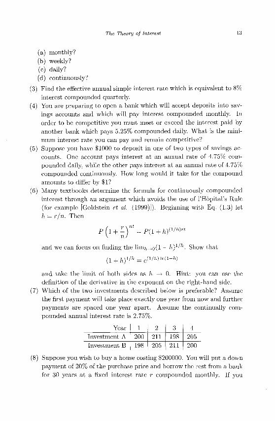
(7) Which of the two investments described below is preferable? Assume the first payment will take place exactly one year from now and further payments are spaced one year apart. Assume the continually compounded annual interest rate is 2.75%.
Year Investment A Investment B
1 200 198
2 211 205
3 198 211
4 205 200
(8) Suppose you wish to buy a house costing $200000. You will put a down payment of 20% of the purchase price and borrow the rest from a bank for 30 years at a fixed interest rate r compounded monthly. If you
14 An Undergraduate Introduction to Financial Mathematics
wish your monthly mortgage payment to be $1500 or less, what is the maximum annual interest rate for the mortgage loan?
(9) Use the Mean Value Theorem (p. 235 of [Stewart (1999)]) to show the rate of return defined by the root of the function in Eq. (1.7) is unique.
(10) Suppose for an investment of $10000 you will receive payments at the end of each of the next four years in the amounts {2000,3000,4000,3000}. What is the rate of return per year?
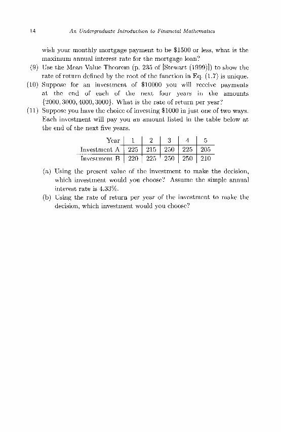
(11) Suppose you have the choice of investing $1000 in just one of two ways. Each investment will pay you an amount listed in the table below at the end of the next five years.
Year
Investment A
Investment B
1
225
220
2
215
225
3
250
250
4
225
250
5
205
210
(a) Using the present value of the investment to make the decision, which investment would you choose? Assume the simple annual interest rate is 4.33%.
(b) Using the rate of return per year of the investment to make the decision, which investment would you choose?
Chapter 2
Discrete Probability
Since the number and interactions of forces driving the values of investments are so large and complex, development of a deterministic mathematical model of a market is likely to be impossible. In this book a probabilistic or stochastic model of a market will be developed instead. This chapter presents some elementary concepts of probability and statistics. Here the reader will find explanations of discrete events and their outcomes. A discrete outcome can take on only one of a finite number of values. For example the outcome of a roll of a fair die can be only one of the six values in the set {1, 2, 3,4, 5,6}. No one ever rolls a die and discovers the outcome to be 7r for example. Basic methods for determining the probabilities of outcomes will be presented. The concept of the random variable, a numerical quantity whose value is not known until an experiment is conducted, will be explained. There are many different kinds of discrete random variables, but one that frequently arises in financial mathematics is the binomial random variable. While statistics is a field of study unto itself, two important descriptive statistics will be introduced in this chapter, expected value (or mean) and standard deviation. The expected value provides a number which is representative of typical values of a random variable, while the standard deviation provides a measure of the "spread" in the values the random variable can take on.
2.1 Events and Probabilities
To the layman an event is something that happens. To the statistician, an event is an outcome or set of outcomes of an experiment. This brings up the question of what is an experiment? For our purposes an experiment will be any activity that generates an observable outcome. Some simple
15
16 An Undergraduate Introduction to Financial Mathematics
examples of experiments include flipping a coin, rolling a pair of dice, and drawing cards from a deck. An outcome of each of these experiments could be "heads", 7, or the ace of hearts respectively. For the example of the coin flip or drawing a card from the deck, the example outcomes given can be thought of as "atomic" in the sense that they cannot be further broken down into simpler events. The outcome of achieving a 7 on a roll of a pair of dice could be thought of as consisting of a pair of outcomes, one for each die. For example the 7 could be the result of 2 on the first die and 5 on the second. Having a flipped coin land heads up cannot be similarly decomposed. An event can also be thought of as a collection of outcomes rather than just a single outcome. For example the experiment of drawing a card from a standard deck, the events could be segregated into hearts, diamonds, spades, or clubs depending on the suit of the card drawn. Then any of the atomic events 2 , 3 , . . . , 10, jack, queen, king, or ace of hearts would be a "heart" event for the experiment of drawing a card and observing its suit.
In this chapter the outcomes of experiments will be thought of as discrete in the sense that the outcomes will be from a set whose members are isolated from each other by gaps. The discreteness of a coin flip, a roll of a pair of dice, and card draw are apparent due to the condition that there is no outcome between "heads" and "tails", or between 6 and 7, or between the two of clubs and the three of clubs respectively. Also in this chapter the number of different outcomes of an experiment will be either finite or countable (meaning that the outcomes can be put into one-to-one correspondence with a subset of the natural numbers).
The probability of an event is a real number measuring the likelihood of that event occurring as the outcome of an experiment. To begin the more formal study of events and probabilities, let the symbol A represent an event. The probability of event A will be denoted P (A). By convention, probabilities are always real numbers in the interval [0,1], that is, 0 < P ( 4) < 1- If -A is an event for which P (A) — 0, then A is said to be an impossible event. If P (A) = 1, then A is said to be a certain event. Impossible events never occur, while certain events always occur. Events with probabilities closer to 1 are more likely to occur than events whose probabilities are closer to 0.
There are two approaches to assigning a probability to an event, the classical approach and the empirical approach. Adopting the empirical approach requires an investigator to conduct (or at least simulate) the experiment N times (where N is usually taken to be as large as practical).
Discrete Probability 17
During the N repetitions of the experiment the investigator counts the number of times that event A occurred. Suppose this number is x. Then the probability of event A is estimated to be P (A) = x/N. The classical approach is a more theoretical exercise. The investigator must consider the experiment carefully and determine the total number of different outcomes of the experiment (call this number M), assume that each outcome is equally likely, and then determine the number of outcomes among the total in which event A occurs (suppose this number is y). The probability of event A is then assigned the value P (A) = y/M. In practice the two methods closely agree, especially when N is very large.
Some experiments involve events which can be thought of as the result of two or more outcomes occurring simultaneously. For example, suppose a red coin and a green coin will be flipped. One compound outcome of the experiment is the red coin lands on "heads" and the green coin lands on "heads" also. The next section contains some simple rules for handling the probabilities of these compound events.
2.2 Addition Rule
Suppose A and B are two events which may occur as a result of conducting an experiment. An investigator may wish to know the probability that A or B occurs. Symbolically this would be represented as P (A V B). If an investigator rolls a pair of fair dice they may want to know the probability that a total or 2 or 12 results. Let event A be the outcome of 2 and B be the outcome of 12. Since P ( 4) = 1/36 and P (B) = 1/36 and the two events are mutually exclusive, that is, they cannot both simultaneously occur, the P ( 4 V B) = P (A) + P (B) = 1/18. Suppose instead that the investigator wants to know the probability that a total of less than 6 or an odd total results. We can let event A be the outcome of a total less than 6 (that is, a total of 2, 3, 4, or 5) and let event B be the outcome of an odd total (specifically 3, 5, 7, 9, or 11). We see this time that events A a.n B are not mutually exclusive, there are outcomes which overlap both events, namely the odd numbers 3 and 5 are less than 6. To adjust the calculation the probabilities of the non-exclusive events should be counted only once. Thus the P(AVB) = P (A) + P (B) - P {A A B) where P (A A B) is the probability that one of the events in the overlapping non-exclusive set of
18 An Undergraduate Introduction to Financial Mathematics
outcomes occurs. Hence
P ( A V B ) = U + 1 8 + 12 + 9j + U + 9- + 6 + 9 + 1 8 j - U + 9 J _ 11 ~ 18'
Thus the calculation of the probability of event A or event B occurring is different depending on whether A and B are mutually exclusive.
The concept outlined above is known as the Addition Rule for Probabilities and can be stated in the form of a theorem.
Theorem 2.1 (Addition Rule) For events A and B, the probability of A or B occurring is
P ( i V B)=P(A)+P(B)-P(A/\B). (2.1)
If A and B are mutually exclusive events then P ( A A B ) = 0 and the Addition Rule simplifies to
P {A V B) = P {A) + P (B).
Determining the probability of the occurrence of A or B rests on determining the probability that both A and B occur. This topic is explored in the next section.
2.3 Conditional Probability and Multiplication Rule
During the past decade a very famous puzzle involving probability has come to be known as the "Monty Hall Problem". This paradox of probability was published in a different but equivalent form in Martin Gardner's "Mathematical Games" feature of Scientific American [Gardner (1959)] in 1959 and in the American Statistician [Selvin (1975)] in 1975. In 1990 it appeared in its present form in the "Ask Marilyn" column of Parade Magazine [vos Savant (1990)].
A game show host hides a prize behind one of three doors. A contestant must guess which door hides the prize. First, the contestant announces the door they have chosen. The host will then open one of the two doors not chosen in order to reveal the prize is not behind it. The host then tells the contestant they may keep their original choice or switch to the other unopened door. Should the contestant switch doors?
Discrete Probability 19
At first glance when faced with two identical unopened doors, it may seem that there is no advantage to switching doors; however, if the contestant switches they will win with probability 2/3. When the contestant makes the first choice they have a 1/3 chance of being correct and a 2/3 chance of being incorrect. When the host reveals the non-winning, unchosen door, the contestants first choice still has a 1/3 chance of being correct, but now the unchosen unopened door has a 2/3 probability of being correct, so the contestant should switch.
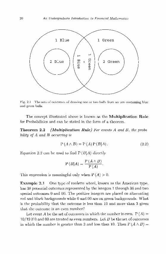
This example illustrates the concept known as conditional probability. Essentially the decision the contestant faces is "given that I have seen that one of the doors I did not choose is not the winning door, should I alter my choice?" The probability that one event occurs given that another event has occurred is called conditional probability. The probability that event A occurs given that event B occurs is denoted P (A\B). One of the classical thought experiments of discrete probability involves selecting balls from an urn. Suppose an urn contains 20 balls, 6 of which are blue and the remaining 14 are green. Two balls will be drawn, the second will be drawn without replacing the first. The question "what is the probability that the second ball is green, given that the first ball was green?" could be asked. The answer to this question will motivate the statement of the multiplication rule of probability. One approach to the answer involves determining the probability that when two balls are drawn without replacement they are both green. The probability that both selections are green would be the number of two green ball outcomes divided by the total number of outcomes. There are 20 candidates for the first ball selected and there are 19 candidates for the second ball selected. Thus the total number of outcomes is 380. Of those outcomes (14) (13) = 182 are both green balls. Thus the probability that both balls are green is 182/380 = 91/190. The reader may be asking what this situation has to do with the question originally posed. The outcome in which both balls are green is a subset of all the outcomes in which the first ball is green. Consider the diagram in Fig. 2.1. Thus the probability that both balls are green is the product of the probability that the first ball is green multiplied the probability the second ball is green. Let event A be the set of outcomes in which the first ball is green and event B be the set of outcomes in which the second ball is green. Numerically P (A) = 7/10 and symbolically
P(AAB) = P(A) P{B\A)
Thus P (B\A) =P(AAB)/P (A) = (91/190)/(7/10) = 13/19.
20 An Undergraduate Introduction to Financial Mathematics
Fig. 2.1 The sets of outcomes of drawing one or two balls from an urn containing blue and green balls.
The concept illustrated above is known as the Multiplication Rule for Probabilities and can be stated in the form of a theorem.
Theorem 2.2 (Multiplication Rule) For events A and B, the probability of A and B occurring is
P(AAB) = P(A)F{B\A). (2.2)
Equation 2.2 can be used to find P (B\A) directly
This expression is meaningful only when P (A) > 0.
Example 2.1 One type of roulette wheel, known as the American type, has 38 potential outcomes represented by the integers 1 through 36 and two special outcomes 0 and 00. The positive integers are placed on alternating red and black backgrounds while 0 and 00 are on green backgrounds. What is the probability that the outcome is less than 10 and more than 3 given that the outcome is an even number?
Let event A be the set of outcomes in which the number is even. P (A) = 10/19 if 0 and 00 are treated as even numbers. Let B be the set of outcomes in which the number is greater than 3 and less than 10. Then P (A A B) =
Discrete Probability 21
3/38 and
p w = S = 3/20' To expand on the previous example, suppose the roulette wheel will
be spun twice. One could ask what is the probability that both spins have a red outcome. If event A is the outcome of red on the first spin and event B is the outcome of red on the second spin, then we as before P (A A B) = P (A) P (B\A). However there is no reason to believe that the wheel somehow "remembers" the outcome of the first spin while is is being spun the second time. The first outcome has no effect on the second outcome. In any experiment, if event A has no effect on event B then A and B are said to be independent. In this situation P (B\A) = P (B). Thus for independent events the Multiplication Rule can be modified to
P(AAB)=P{A)P (B).
Therefore the probability that both spins will have red outcomes is P(AAB) = (9/19)(9/19) = 81/361.
2.4 Random Variables and Probability Distributions
The outcome of an experiment is not known until after the experiment is performed. For example the number of people who vote in an election is not known until the election is concluded. In a more formal sense we can describe a random variable as a function which maps the set of outcomes of an experiment to some subset of the real numbers. In the election example (assuming the number of registered voters is N and that there will be no fraudulent voting) the sample space of outcomes of voter turnout is the set S = {0 ,1 ,2 , . . . , N}. Symbolically a random variable for the voter turnout is the function X : S —> M. Often X is thought of as the eventual numeric result of the experiment.
A probability distribution is a function which assigns a probability to each element in the sample space of outcomes of an experiment. If S is the set outcomes of an experiment and / is the associated probability distribution function, then / maps each element in 5 to a unique real number in the interval [0,1]. If a; is a potential outcome of an experiment with sample space S then f(x) = P (X = x), in other words f(x) is the probability that x occurs as the outcome of the experiment. Since a probability
22 An Undergraduate Introduction to Financial Mathematics
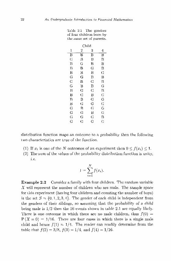
Table 2.1 T h e genders of four children bo rn by the same set of paren ts .
1 B G B B B G G G B B B B G G G G
Child 2 B B G B B G B B G G B G B G G G
3 B B B G B B G B G B G G G B G G
4 B B B B G B B G B G G G G G B G
distribution function maps an outcome to a probability then the following two characteristics are true of the function.
(1) If Xi is one of the N outcomes of an experiment then 0 < / ( X J ) < 1. (2) The sum of the values of the probability distribution function is unity,
i.e.
N
Example 2.2 Consider a family with four children. The random variable X will represent the number of children who are male. The sample space for this experiment (having four children and counting the number of boys) is the set S = {0,1,2,3,4}. The gender of each child is independent from the genders of their siblings, so assuming that the probability of a child being male is 1/2 then the 16 events shown in table 2.1 are equally likely. There is one outcome in which there are no male children, thus /(0) = P (X = 0) = 1/16. There are four cases in which there is a single male child and hence / ( l ) = 1/4. The reader can readily determine from the table that /(2) = 3/8, /(3) = 1/4, and /(4) = 1/16.
Discrete Probability 23
Several common types of random variables and their associated probability distributions will be important to the study of financial mathematics. The binomial random variable will be discussed in the next section. It will be seen to be related to the Bernoulli random variable which takes on only one of two possible values, often thought of as true or false (or sometimes as success and failure). It is mathematically convenient to designate the outcomes as 0 and 1. The probability distribution function of a Bernoulli random is particularly simple, / ( l ) = P (X = 1) = p where 0 <p< 1 and /(0) = I-p.
2.5 Binomial Random Variables
Returning to the last example of the previous section, we can think of the births of four children as four independent events. The gender of one child in no way influences the genders of children born before or after. Since the gender of a child can take on only one of two values it is possible to think of the birth of each child as a Bernoulli event. The probability of having a male or female child does not change between births. Thus the experiment of producing four children in a family is the same as repeating the experiment of having a single child four times or, repeating a Bernoulli experiment four times. This is the idea of the binomial random variable defined next. A binomial random variable X is the number of successful outcomes out of n independent Bernoulli random variables.
A binomial random variable is parameterized by the number of repetitions of the Bernoulli experiment (referred to as trials from here on) and by the probability of success on a single trial. If the number of trials is n and the probability of success on a single trial is p, then the set of possible outcomes of the binomial experiment is the set { 0 , 1 , . . . , n}. The number of combinations of x successes out of n trials is
\x) x\(n — x)\
The probability of x successes out of n independent trials in a specified combination is, according to the Multiplication Rule, ^ ( 1 — p)n~x. Since the various combinations are mutually exclusive, by the Addition Rule the probability of x successes out of n trials is given by the function
P(X=x)= y ^ ( l -p)»- = - ^ _ ^ * ( i _ p r - (2.3)
24 An Undergraduate Introduction to Financial Mathematics
Thus if the probability of an individual child being born male or female is 1/2, the probability that a family with four children will have two female children is
This result agrees with the result of the more cumbersome method used to determine this probability in the previous section.
Example 2.3 The probability that a computer memory chip is defective is 0.02. A SIMM (single in-line memory module) contains 16 chips for data storage and a 17th chip for error correction. The SIMM can operate correctly if one chip is defective, but not if two or more are defective. The probability that a SIMM will not function is
17 / 1 7 \ p (X > 2) = J2 I J (0.02)a:(0.98)17-a: w 0.044578.
2.6 Expected Value
When faced with experimental data, summary statistics are often useful for making sense of the data. In this context "statistics" refers to numbers which can be calculated from the data rather than the means and algorithms by which these numbers are calculated. In financial mathematics the statistical needs are somewhat more specialized than in a general purpose course in statistics. Here we wish to answer the hypothetical question, "if an experiment was to be performed an infinite number of times, what would be the typical outcome?" Thus we will introduce only the statistical concepts to be used later in this text. A reader interested in a broader, deeper, and more rigorous background in statistics should consult one of the many textbooks devoted to the subject for example [Ross (2006)].
To take an example, if a fair die was rolled an infinite number of times, what would be the typical result? The notion to be explored in this section is that of expected value. In some ways expected value is synonymous with the mean or average of a list of numerical values; however, it can differ in at least two important ways. First, the expected value usually refers to the typical value of a random variable whose outcomes are not necessarily equally likely whereas the mean of a list of data treats each observation as equally likely. Second, the expected value of a random variable is the
Discrete Probability 25
typical outcome of an experiment performed an infinite number of times whereas the statistical mean is calculated based on a finite collection of observations of the outcome of an experiment.
If X is a discrete random variable with probability distribution P (X) then the expected value of X is denoted E [X] and defined as
E[X] = £ ( X - P p O ) . (2.4) x
It is understood that the summation is taken over all values that X may assume. In the case that X takes on only a finite number of values with nonzero probability, then this sum is well-defined. If X may assume an infinite number of values with probabilities greater than zero, we will assume that the sum converges. Since each value of X is multiplied by its corresponding probability, the expected value of X is a weighted average of the variable X. Returning to the question posed in the previous paragraph as to the typical outcome achieved when rolling a fair die an infinite number of times, we may determine this number from the formula for expected value. Since X G {1,2,3,4, 5,6} and P (X) = 1/6 for all possible values of X, then the expected value of X is
E[x] = ±x = 1-±x = 1-.mi = i. 1 J ^ 6 6 ^ 6 2 2
x=i x=i Thus the average outcome of rolling a fair die is 3.5.
Example 2.4 Let random variable X represent the number of female children in a family of four children. Assuming that births of males and females are equally likely and that all births are independent events, what is the E [X]? The sample space of X is the set {0,1,2,3,4}. Using the binomial probability formula P (0) = 1/16, P (1) = 1/4, P (2) = 3/8, P (3) = 1/4, and P (4) = 1/16, we have
E[X] = 0. 1 + 1. I + 2 - I + 3- ± + 4 - 1 = 2.
In families having four children, typically there are two female children and consequently two male children.
The notion of the expected value of a random variable X can be extended to the expected value of a function of X. Thus we say that if F is
26 An Undergraduate Introduction to Financial Mathematics
a function applied to X, then
E[F(X)]=Y,F(X)P(X). x
When the function F is merely multiplication by a constant then the expected value takes on a simple form.
Theorem 2.3 If X is a random variable and a is a constant, then E[aX] =aE[X}.
Proof. By the definition of expected value
E [aX] = £ daX) • P PO) =aJ2(X-P (X)) = aE [X].
a
Later in this work sums of random variables will become important. Thus some attention must be given to the expected value of the sum of random variables. However, this requires the probability of two or more random variables be considered simultaneously. The reader should already be familiar with one example of this situation, namely the rolling of a pair of dice. Suppose that the two dice can be distinguished from one another (imagine that one of them is red while the other is green). Let X be the random variable denoting the outcome of the green die while Y is a random variable denoting the outcome of the red die. If the experiment to be performed is rolling the pair of dice and considering the total of the upward faces then the random variable denoting the outcome of this experiment is X + Y. This naturally leads us to the issue of describing the probabilities associated with various values of the random variable X + Y. The joint probability function is denoted P (X, Y) and we will understand it to mean P (X, Y) = P (X A Y). Thus P (1, 3) symbolizes the probability that the outcome of the red die is 1 while the outcome of the green die is 3. If the individual dice are independent then P ( l , 3 ) = P(1)P(3) = 1/36 according to the multiplication rule. A couple of additional comments are in order. First, joint probabilities exist even for random events which are not independent. Second, realize that in general P (X + Y) / P (X) + P (Y). This is an abuse of notation, but is not likely to cause confusion in what follows. P (X + Y) refers to the probability of the sum X+Y which depends on the joint probabilities of X and Y. P (X) and P (Y) refer respectively to the individual probabilities of random variable X and Y. The following is true, if we wish to know the probability that the sum of the discrete random
Discrete Probability 27
variables X and Y is m then by using the addition rule for probabilities
P{X + Y = m) = J2 P(X>Y)-X+Y=m
The summation is taken over all combinations of X and Y such that X + Y — m. Returning to the dice example introduced earlier in the paragraph we see that the probability that the sum of the dice is 4 is
P(X + Y = A) = Y^ p(X'Y) X+Y=4
= P(1,3) + P(2,2) + P(3,1) _ 1_ 1 J_ _ 1_ _ 3 6 + 36 + 3 6 ~ 1 2 '
The joint probability distribution of a pair of random variables possesses many of the same properties that the probability distribution of a single random variable possesses. For example 0 < P (X, Y) < 1 for all X and Y in the discrete sample space. It is also true that
££p(x,r) = ££p(*,n = i. X Y Y X
An important property will be used in the proof of the next theorem. The sum of the joint probability of X and Y where Y is allowed to take on each of its possible values is called the marginal probability of X. Without confusion we will denote the marginal probability of X as P (X) and realize that
ppO = £p (x ,y ) . Y
Similarly the marginal probability of Y is denoted P (Y) and defined as
P ( F ) = £ P ( X , r ) . x
Conveniently the expected value of a sum of random variables is the sum of the expected values of the random variables. This notion is made more precise in the following theorem.
Theorem 2.4 If Xi,X2, • •. ,Xk are random variables then
E [Xi + X2 + • • • Xk] = E [Xi] + E [X2] + • • • + E [Xk].
28 An Undergraduate Introduction to Financial Mathematics
Proof. If k = 1 then the proposition is certainly true. If k = 2 then
E[X1+X2]= J2 ((X1+X2)F(X1,X2)) X\ ,X2
= EE« x i+ x 2)p(*i ,* 2 ) ) X1 X2
= ^ ^ X 1 P ( X l l X 2 ) + ^ ^ l 2 P ( l 1 ) X 2 ) X\ X2 X2 X\
X\ X2 X2 Xi
= ]Tx1P(X1) + ^X 2 P(X 2 ) X1 X2
= E [X^ + E [X2] •
For a finite value of k > 2 the result is true by induction. Suppose the result is true for n < k where k > 2, then
E ^ + • • • + Xk_i + Xfc] = E [Xi + • • • + Xfc_i] + E [Xk]
= E [X^ + • • • + E [Xfc_i] + E [jffc]
The last step is true by the induction hypothesis. •
We can use Theorem 2.4 to determine the expected value of a binomial random variable. Along the way we will also find the expected value of a Bernoulli random variable. Suppose n trials of a Bernoulli experiment will be conducted for which the probability of success on a single trial is 0 < p < 1. Random variable X represents the number of successes out of n trials. By assumption the trials are independent of one another and the outcomes are mutually exclusive. The result of the binomial experiment can be thought of as the sum of the results of n Bernoulli experiments. Let the random variable Xi be the number of successes of the ith Bernoulli trial, then
E [X] = E [Xi + • • • + Xn] = E [Xi] + • • • + E [Xn] =p+---+p = np.
Later we will have need to calculate the expected value of a product of random variables. This situation is not as straightforward as the case of a sum of random variables.
Theorem 2.5 Let Xi, X2, ... ,Xk be pairwise independent random vari-
Discrete Probability 29
ables, then
E [XXX2 •••Xk] = E [X^ E [X2] • • • E [Xfc].
Proof. Naturally we see that when k = 1 the theorem is true. Next we will consider the case when k = 2. Let X\ and X2 be independent random variables with joint probability distribution P (X±, X2)- Since the random variables are assumed to be independent then P {X\, X2) = P {X\) P (X2). Once again we are lax in our use of notation, since in the previous equation the symbol P is used in three senses ((1) the joint probability distribution of X\ and X2, (2) the probability distribution of X\, and (3) the probability distribution of X2)\ however, there is little chance of confusion in this elementary proof.
E[X1X2} = J2 X1X2P(X1,X2) X\,X2
= EEM2P(X!)P(X2) X\ X2
= ^ X 1 P ( X 1 ) ^ X 2 P ( X 2 ) X\ X2
= E [XJ E [X2\
For a finite value of k > 2 the result is true by induction. Suppose the result is true for n < k where k > 2, then
E [X\ • • • Xk-iXk] = E [X\ • • • Xk-i] E [Xk]
= E[X1]---E[Xk-1]E[Xk]
The last step is true by the induction hypothesis. •
The expected value of a random variable specifies the average outcome of an infinite number of repetitions of an experiment. In the next section the notions of variance and standard deviation are introduced. They specify measures of the spread of the outcomes from the expected value.
2.7 Variance and Standard Deviation
The variance of a random variable is a measure of the spread of values of the random variable about the expected value of the random variable. The
30 An Undergraduate Introduction to Financial Mathematics
variance is defined as
V a r ( X ) = E [ ( X - E [ X ] ) 2 ] (2.5)
As the reader can see from Eq. (2.5), the variance is always non-negative. The expression X — E [X] is the signed deviation of X from its expected value. The variance may be interpreted as the average of the squared deviation of a random variable from its expected value. An alternative formula for the variance is sometimes more convenient in calculations.
Theorem 2.6 Let X be a random variable, then the variance of X is E[X2] -E[X}2.
Proof. By definition,
Var(X) = E [ ( X - E [ X ] ) 2
E X2 - 2XE [X] + E [X]2
E [X2] - E [2XE [X]] + E | E [X]2
E [X2] - 2E [X] E [X] + E [X]2
E [X2] - E [X]2 .
The third and fourth steps of this derivation made use of theorems 2.4 and 2.3 respectively. •
Returning to the previous example of the hypothetical family with four children, we can now investigate the variance in the number of female children. We already know that E [X] — 2. If we make use of the result of Theorem 2.6 then
Var(X) = E [ X 2 ] - E [X]2
= (02)(1/16) + ( l 2)( l /4) + (22)(3/8) + (32)(l/4) + (42)(1/16) - 22
= 1.
Before investigating the variance of a binomial random variable, we should determine the variance of a Bernoulli random variable. If the prob-
Discrete Probability 31
ability of success is 0 < p < 1 then according to Eq. (2.5),
Var(X) = E [ ( X - E [ X ] ) 2 ]
= E[(X-p)2] = ( I - P ) 2 P + ( O - P ) 2 ( I - P )
= (l-p)2p + p2(l-p)
= p(l - p)(l - p + p)
= p(l -p).
The following theorem provides an easy formula for calculating the variance of independent random variables.
Theorem 2.7 Let X\, X2, • • •, X^ be pair-wise independent random, variables, then
Var (Xi + X2 + • • • + Xk) = Var (X :) + Var (X2) + • • • + Var (Xfc).
Proof. If k = 1 then the result is trivially true. Take the case when k = 2. By the definition of variance,
Var (Xi + X2) = E [((Xi + X2) - E [Xi + X2])2]
= E [ ( ( X 1 + X 2 ) - E [ X 1 ] - E [ X 2 ] ) 2 ]
= E [((Xi - E [Xi]) + (X2 - E [X2]))2]
= E [(X! - E [X!])2 + (X2 - E [X2])2 +
2 ( X 1 - E [ X 1 ] ) ( X 2 - E [ X 2 ] ) ]
= E [(Xi - E [X!])2] + E [(X2 - E [X2])2] +
2 E [ ( X 1 - E [ X 1 ] ) ( X 2 - E [ X 2 ] ) ]
= Var (Xi) + Var (X2) + 2E [(Xi - E [X1])(X2 - E [X2])]
Since we are assuming that random variables X\ and X2 are independent, then by Theorem 2.5
E [(X1 - E [X1])(X2 - E [X2])] = E [Xx - E [Xx]] E [X2 - E [X2]]
= ( E [ X 1 ] - E [ X 1 ] ) ( E [ X 2 ] - E [ X 2 ] )
= 0,
and thus
Var (Xi + X2) = Var ( X ^ + Var (X 2 ) .
32 An Undergraduate Introduction to Financial Mathematics
The result can be extended to any finite value of k by induction. Suppose the result has been shown true for n < k with k > 2. Then
Var (X1 + • • • + Xk_! + Xk) = Var (Xi + • • • + Xfc_i) + Var (Xk)
= Var (Xi) + • • • + Var (Xk^) + Var (Xk)
where the last equality is justified by the induction hypothesis. •
Readers should think carefully about the validity of the claim that X\ — E [Xi] and X2 — E [X2] are independent in light of the assumption that X\ and X2 are independent.
Example 2.5 Suppose a binomial experiment is characterized by n independent repetitions of a Bernoulli trial for which the probability of success on a single trial is 0 < p < 1. Random variable X denotes the total number of successes accrued over the n trials.
Var {X) = Var ^ Xj
= y Var (Xj) (since trials are independent) i= i
= f>(l-p)
= np(l — p)
So far we have made no mention of the other topic in the heading for this section, namely standard deviation. There is little more that must be said since by definition the standard deviation is the square root of the variance. Standard deviation of a random variable X is denoted by a (X) and thus
a{X) = VVar(X).
2.8 Exercises
(1) Suppose the four sides of a regular tetrahedron are labeled 1 through 4. If the tetrahedron is rolled like a die, what is the probability of it landing on 3?
Discrete Probability 33
(2) Use the classical approach and the assumption of fair dice to find the probabilities of the outcomes obtained by rolling a pair of dice and summing the dots shown on the the upward faces.
(3) If the probability that a batter strikes out in the first inning of a baseball game is 1/3 and the probability that the batter strikes out in the fifth inning is 1/4, and the probability that the batter strikes out in both innings is 1/10, then what is the probability that the batter strikes out in either inning?
(4) Part of a well-known puzzle involves three people entering a room. As each person enters, at random either a red or a blue hat is placed on the person's head. The probability that an individual receives a red hat is 1/2. No person can see the color of their own hat, but they can see the color of the other two persons' hats. The three will split a prize if at least one person guesses the color of their own hat correctly and no one guesses incorrectly. A person may decide to pass rather than to guess. The three people are not allowed to confer with one another once the hats have been placed on their heads, but they are allowed to agree on a strategy prior to entering the room. At the risk of spoiling the puzzle, one strategy the players may follow instructs a player to pass if they see the other two persons wearing mis-matched hats and to guess the opposite color if their friends are wearing matching hats. Why is this a good strategy and what is the probability of winning the game?
(5) Suppose cards will be drawn without replacement from a standard 52-card deck. What is the probability that the first two cards will be aces?
(6) Suppose cards will be drawn without replacement from a standard 52-card deck. What is the probability that the second card drawn will be an ace and that the first card was not an ace?
(7) Suppose cards will be drawn without replacement from a standard 52-card deck. What is the probability that the fourth card drawn will be an ace given that the first three cards drawn were all aces?
(8) Suppose cards will be drawn without replacement from a standard 52-card deck. On which draw is the card mostly likely to be the first ace drawn?
(9) On the last 100 spins of an American style roulette wheel, the outcome has been black. What is the probability of the outcome being black on the 101st spin?
34 An Undergraduate Introduction to Financial Mathematics
(10) On the last 5000 spins of an American style roulette wheel, the outcome has been 00. What is the probability of the outcome being 00 on the 5001st spin?
(11) Suppose that a random variable X has a probability distribution function / so that f(x) = c/x for a; = 1, 2 , . . . , 10 and is zero otherwise. Find the appropriate value of the constant c.
(12) Suppose that a box contains 15 black balls and 5 white balls. Three balls will be selected without replacement from the box. Determine the probability distribution function for the number of black balls selected.
(13) Quality control for a manufacturer of integrated circuits is done by randomly selecting 25 chips from the previous days manufacturing run. Each of the 25 chips is tested. If two or more chips are faulty, then the entire run is discarded. Previously gathered evidence indicates that the defect rate for chips is 0.0016. What is the probability that a manufacturing run of chips will be discarded?
(14) The probabilities of a child being born male or female are not exactly equal to 1/2. Typically there are nearly 105 live male births per 100 live female births. Determine the expected number of female children in a family of 6 total children using these birth ratios and ignoring infant mortality.
(15) Suppose a standard deck of 52 cards is well shuffled and one card at a time will be drawn without replacement from the deck. What is the expected value of the first ace drawn (in other words, of the first, second, third, etc cards drawn, on average which will be the first ace drawn)?
(16) Show that for constants a and b and discrete random variable X that E [aX + b] = aE [X] + b.
(17) For the situation described in exercise 15 determine the variance in the occurrence of the first ace drawn.
(18) Show that for constants a and b and discrete random variable X that Var(aX + 6 )=a 2 Var (X) .
Chapter 3
Normal Random Variables and Probability
Whereas in Chapter 2 random variables could take on only a finite number of values taken from a set with gaps between the values, in the present chapter, continuous random variables will be described. A continuous random variable can take on an infinite number of different values from a range without gaps. Calculus-based methods for determining the expected value and standard deviation of a continuous random variable will be described. A very useful type of continuous random variable for the study of financial mathematics is the normal random variable. We will see that when many random factors and influences come together (as in the complex situation of a financial market), the sum of the influences can be modeled by a normal random variable. Finally we will examine some stock market data and detect the presence of normal randomness in the fluctuations of stock prices.
3.1 Continuous Random Variables
Our understanding of probability must change if we are to understand the differences between discrete and continuous random variables. Suppose we consider the interval [0,1]. If we think of only the integers contained in this interval, then only the discrete set {0,1} need be considered. If the probability of selecting either integer from this set is 1/2 then we remain in the realm of discrete probability, random variables, and distributions. If we think of selecting, with equal likelihood, a number from the interval [0,1] of the form k/10 where k G { 0 , 1 , . . . , 10}, then once again our approach to probability remains discrete. The P (X = k/10) = j ^ . Continuing in this way we see that if consider only the real numbers in [0,1] of the form k/n where k e { 0 , 1 , . . . , n}, then P (X = k/n) = ^ - . So long as n is finite we
35
36 An Undergraduate Introduction to Financial Mathematics
are dealing with the familiar concept of discrete probability. What happens as n —» oo? In one sense we can think of this limiting case as the case of continuous probability. We say continuous because in the limit, the gaps between the outcomes in the sample space disappear. However, if we retain the old notion of probability, the likelihood of choosing a particular number from the interval [0,1] becomes
lim = 0. n ^ o c n + 1
This is correct but brings to mind a paradox. Does this imply that the probability of choosing any number from [0,1] is 0? Surely we must choose some number. What is needed is a shift in our notion of probability when dealing with continuous random variables. Instead of determining the probability that a continuous random variable equals some real number, the meaningful determination is the likelihood that the random variable lies in a set, usually an interval or finite union of intervals on the real line. These notions are defined next.
A random variable X has a continuous distribution if there exists a non-negative function / : M —» K such that for an interval [a, b] the
P (a < X < b) = f f(x) dx. (3.1) J a
The function / which is known as the probability distribution function must, in addition to satisfying f(x) > 0, have the following property,
/
oo
f(x)dx = l. (3.2)
-oo
These properties are the analogues of properties of discrete random variables and their distributions. The probabilities of individual values of the random variable are non-negative. In fact, as explained above P (X = x) = 0 for a continuous random variable provided /(£) is continuous at t = x. By contrast P (X = x) can be greater than zero for a discrete random variable. The sum, expressed now as an integral over the real number line, of the values of the probability distribution function must be one. Interpreted graphically, if X represents a continuous random variable then P (a < X < b) represents the area of the region bounded by the graph of the probability distribution function, the x-axis, and the lines x = a and x = b. See Fig. 3.1. The total area under the graph of the probability density function is unity.
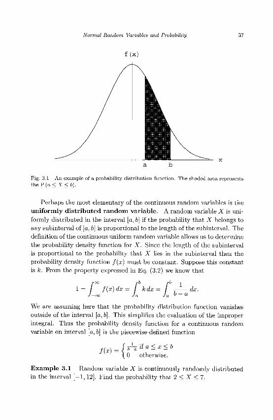
Normal Random Variables and Probability 37
f (X)
Fig. 3.1 An example of a probability distribution function. The shaded area represents the P ( a < X < b).
Perhaps the most elementary of the continuous random variables is the uniformly distributed random variable. A random variable X is uniformly distributed in the interval [a, b) if the probability that X belongs to any subinterval of [a, b] is proportional to the length of the subinterval. The definition of the continuous uniform random variable allows us to determine the probability density function for X. Since the length of the subinterval is proportional to the probability that X lies in the subinterval then the probability density function f{x) must be constant. Suppose this constant is k. From the property expressed in Eq. (3.2) we know that
/
o o t>b /•& -i
f(x) dx = / kdx = dx. -oo J a J a b ~ a
We are assuming here that the probability distribution function vanishes outside of the interval [a, b]. This simplifies the evaluation of the improper integral. Thus the probability density function for a continuous random variable on interval [a, b] is the piecewise-defined function
TT— if a < x < b b—a — —
0 otherwise.
Example 3.1 Random variable X is continuously randomly distributed in the interval [-1,12]. Find the probability that 2 < X < 7.
m
38 An Undergraduate Introduction to Financial Mathematics
Since according to the previous discussion of uniformly distributed random variables, the probability density function of X is
we have
^ if - 1 < x < 12 0 otherwise,
P(2<X<7) = J f(x)dx = J i 2 1 3 d x 13
Now that continuous random variables and their probability distributions have been introduced we can begin to discuss formulae for determining their means and variances.
3.2 Expected Value of Continuous Random Variables
By definition the expected value or mean of a continuous random variable with probability density function f(x) is
/>00
E [X] = / xf{x) dx. (3.3)
This equation is analogous to Eq. (2.4) for the case of a discrete random variable. In the continuous case the product of the value of the random variable and its probability density function is summed (this time through the use of a definite integral) over all values of the random variable. The expected value is only meaningful in cases in which the improper integral in (3.3) converges.
Example 3.2 Find the expected value of X if X is a continuously uniformly distributed random variable on the interval [—50, 75].
Using Eq. (3.3) we have
The results which follow in this section will be similar to the results that were presented for discrete random variables. In most cases the notion of a discrete sum need only be replaced by a definite integral to justify these new results. To keep the exposition as brief as possible, many of the proofs of results in this section will be left to the reader. The expected value of
Normal Random Variables and Probability 39
a function g of a continuously distributed random variable X which has probability distribution function / is denned as
E /
OO
g(x)f(x)dx, (3.4) -OO
provided the improper integral converges absolutely, i.e., E [<?(X)] is denned if and only if
/"OO
\g(x)\f(x)dx < oo.
Joint probability distributions for continuous random variables are defined similarly to those for discrete random variables. A joint probability distribution for a pair of random variables is a non-negative function f(x, y) for which
pOO rOO
/
OO /-OO
/ f{x,y)dxdy.
Consequently the expected value of a function g : E 2 —> R of the two random variables X and Y is defined as
/
oo /«oo
/ g(x,y)f(x,y)dx -oo J — oo
dy,
again, provided the integral is absolutely convergent.
Example 3.3 Consider the jointly distributed random variables (X, Y) £ [l,oo] x [—1,2] whose distribution is the function f(x,y) = g|g-. We can find the mean of X + Y as follows.
/
OO />00 r\
\ (x + y)-1dxdy -oo J — oo "•*•'
o2 y o o /
Z />00 rt
LI Bdxdy+Ll Bdxdy
f°° f2 2x , , Z2 f°° 2y , ,
k L^dydx+Lk ^dxdy 2y - i 3
1 5
/•°° 2 3k ^^ 2 ,
2 2
40 An Undergraduate Introduction to Financial Mathematics
If we examine the example above we recognize that E [X + Y] = E [X] + E\Y]. This is true in general, not just for the previous example. The additivity property of the expected value of continuous random variables is stated in the following theorem.
Theorem 3.1 If X\,X2,- • • ,Xk are continuous random variables with joint probability distribution f(x\,x2, • • •, Xfc) then E [Xi + X2 + • • • Xk] = E[X1]+E[X2} + --- + E[Xk}.
The reader should again note that, just as was the case in the previous chapter, the previous theorem is true for random variables which are dependent or independent. Before turning our attention to products of continuous random variables we will define the notion of a marginal distribution. If X and Y are continuous random variables with joint distribution f(x,y) then the marginal distribution for X is defined as the function
/
oo f(x,y)dy.
-oo
The marginal distribution for Y is defined similarly. By definition two continuous random variables are independent if the joint distribution factors as the product of the marginal distributions of X and Y.
f(x,y) =g(x)h(y)
This property is used in the proof of the following theorem.
Theorem 3.2 Let X\, X2, • • •, Xk be pairwise independent random variables with joint distribution f(xi,X2, • • •, %k), then
E[X1X2--- Xk] = E [Xi] E [X2] • • • E [Xk].
Just as was the case for discrete random variables in the previous chapter, the expected value of a continuous random variable can be thought of as the average value of the outcome of an infinite number of experiments. The variance and standard deviation of a continuous random variable again mirror the concept earlier defined for discrete random variables.
3.3 Variance and Standard Deviation
The variance of a continuous random variable is a measure of the spread of values of the random variable about the expected value of the random
Normal Random Variables and Probability 41
variable. The variance is denned as
/
oo {x-fi)2f(x)dx, (3.5)
-oo
where jj, = E [X] and f(x) is the probability distribution function of X. The variance may be interpreted as the squared deviation of a random variable from its expected value. An alternative formula for the variance is given in the following theorem.
Theorem 3.3 Let X be a random variable with probability distribution f and mean [i, then the variance of X is E [X2~\ — /i2.
Example 3.4 Find the variance of the continuous random variable whose probability distribution is given by
f 2a; if 0 < x < 1, f (x) = \
[ 0 otherwise.
The reader may readily check that fi = E [X] = 2/3. Now by use of Theorem 3.3 we have
Var {X) / x2(2x)dx-J — oo
f1 , 4 / 2x3 dx- -Jo 9
/ 2x3 dx - - = Jo 9
(1)'
1 4 2 ~ 9 ~
1 18
In the exercises the reader will be asked to prove the following two theorems which extend to continuous random variables results we have already seen for discrete random variables.
Theorem 3.4 Let X be a continuous random variable with probability distribution f(x) and let a,b £ l , then
Var (aX + b) = a2Var (X).
Theorem 3.5 Let X\, X2, • • •, Xk be pairwise independent continuous random variables with joint probability distribution f{xi,X2,..., Xk), then
Var {Xx + X2 + • • • + Xk) = Var {Xx) + Var (X2) + • • • + Var (Xk).
By definition the standard deviation of a continuous random variable is the square root of its variance. The standard deviation is sometimes
42 An Undergraduate Introduction to Financial Mathematics
denoted a. On occasion we will denote the variance of a random variable as a2.
3.4 Normal Random Variables
For our purposes one of the most important and useful continuous random variables will be the normally distributed random variable. A continuous random variable obeying a normal distribution is frequently said to follow the "bell curve". Many measurable quantities found in nature seem to have normal distributions, for example adult heights and weights. Statisticians, mathematicians, and physical scientists frequently assume any quantity subject to a large number of small independently acting forces (regardless of their distributions) is normally distributed. The normal distribution even finds its way into the financial arena via the assumption that movements in the price of an asset are subject to a large number of incompletely understood political, economic, and social forces, thus justifying the assumption that these changes in value are related to a normal random variable (this assumption will be explored further later).
The normal random variable can also be thought of as the limiting behavior of the binomial random variable introduced in Chapter 2. We will explore the derivation of the probability distribution for the normal random variable in this section. This derivation is outlined in [Bleecker and Csordas (1996), pg. 139]. We begin by supposing that a particle sits at the origin of the x-axis and may move the left or the right a distance Ax in a time interval of length At. The (discrete) probability of moving left is 1/2 which also happens to be the probability of moving right. We will show that if n € N and m e Z with — n < m <n and if n — m is even then the probability that the particle is at location X = mAx at time t = nAt is
n ! ( i ) n , N
( i (n + m ) ) ! ( i ( n - m ) ) ! ' V ' '
We will assume that all the steps taken by the particle are independent and identically distributed. Let the total number of steps taken be n and the number of steps taken to the right be r. Consequently the number of steps taken to the left will be n — r. The position of the particle after n steps will be
(r — (n — r))Ax = (2r — n)Ax = mAx,
Normal Random Variables and Probability 43
where we have assigned m~2r-n. Using the binomial probability distribution given in Eq. (2.3) we can state that the probability that the particle is at position mAx after n steps is
P (X = mAx) = P (X = (2r - n)Ax)
(n\( [r)\
n\
r\(n -
'iy ,2)
1 -r)! '
n!
_
UJ m» UJ (I)"
(\{n + m))\ ( | ( n - m ) ) !
since n + m = 2r. This is the same probability as in Eq. (3.6). This claim can also be proved by induction on n. If n = 1 then m = ±1
(the particle is not allowed to remain in place).
1 1U1)1
P(X = -Ax)- - 'K2>
P (X = Ax)
2 (1 (1+ ( - ! ) ) ) ! ( 1 ( 1 - ( _ ! ) ) ) !
2 ( I ( i + i))! ( i ( i - i ) ) !
Thus the claim is true for n = 1. Now suppose the claim is true for fc < n—1. If the particle will move to mAx at time nAt, then at time (n — l)At the particle must be at either (m — l)Ax or (m + l)Air. Therefore at time t = nAt
P (X = mAx) = - P (X = (m - l)Ax) + - P (X = (m + l)Ax)
1 / ( " - 1 ) ! ( | ) rc-1
2 ^ ( i (n - 1 + m - 1))! (±(n - 1 - (m - 1)))!^/
2 ^ ( | ( n - l + m + l ) ) ! ( i ( n - l - ( m + l)))! /
( n - ! ) ! ( ! ) "
( i ( n + m ) ) ! ( i ( n _ m _ 2 ) ) !
I ( n - l ) ! ( | ) n
(±(n + m - 2 ) ) ! ( ± ( n - m ) ) !
»' (r (I(„ + m))!( i (n-m))! '
44 An Undergraduate Introduction to Financial Mathematics
which is the probability given in expression (3.6). Next we will make use of Stirling's Formula which approximates n\ when
n is large.
n! « V2^e~nnn+1/2 (3.7)
If we apply this formula to every factorial present in expression (3.6) we obtain the following sequence of equivalent expressions.
2Tre-nnn+1/2 (±)T
2ne' - ( n + m ) / 2 ( i ( n + m ) ) (n + m + l ) / 2
,71 + 1/2 (1
2 ^ e - ( n - m ) / 2 ( i ( n - m ) ) ( " t + l ) / 2
(hY v^f(I(n + m ) ) ( ^ i + l ) / 2 n
( ^ ( « - m ) ) ( n - m + l ) / 2
1+1/2
2TT (n + m)(™+m+1)/2(n - m ) ( n - m + 1 ) / 2
2 n ( n + m + l ) / 2 n ( r a - m + l ) / 2
/2mr (n + m)(n+m + 1) /2(n - m ) ( n - m + 1 ) / 2
N ( n+m+l ) /2 / „ \ (n-m+l)/2
<2n-K \n + m 2
= 11 + n
>2nix
2
(1 + £) - (n+m+l ) /2
( ' " ! )
TO
, 1 + — /2n7T V n
-m/2
1 TON"1/2
n /
- ( n - m + l ) / 2
2 \ - ( n + l ) / 2
n2
Now we will make use of the fact that m = xjAx and n = t) At. The last expression above is then equal to
l + t / A t
2VA£ \/2?rt
x A A 2A* / x A A 2 A * / + tA J V ~^W I
xAi £Ax
We will suppose the square of the step size along the x-axis is related to the step size in t via the formula (Ax)2 = 2kAt. Using this relationship to replace the At's in the expression above yields
= 1 + —-Ax 1 •Mt V 2kt J V 'hnt
X . \ 2Ax • ^ - & x 2kt 2kt
Ax ( A i ) '
So far what we have derived is an approximation (which we will treat as an equality for large n or, what is equivalent, for small Ax) for the probability that the particle is located at position x = mAx at time t = nAt. To derive
Normal Random Variables and Probability 45
a probability distribution for a continuously distributed random variable we must divide the expression above by 2Ax and take the limit as Ax —> 0. Readers accustomed to numerical approximations for derivatives will recognize that we have used the centered difference formula for the first derivative in order to develop a difference quotient whose limit will be the probability distribution. Background information on finite difference approximations to derivatives can be found in [Burden and Faires (2005)]. We will make use of the result that limAa;^o(l + aAx)l/^x = ea. Let us define f(x,t) as
f(x,t)
1 / , X A \ 5Z^ /- , X A \ 22^ / = — 7 = lim 1 + ^ - A x 1 - —-Ace 1
2\fkrt Ax^o V 2kt J \ 2kt J \
= 2~7kTt^^(e_5ll)f (e"^) 2
We must verify that this expression satisfies the properties of a probability distribution function. For k, t > 0 the expression is non-negative. Since for \x\ > 1 it is true that 0 < e~x < e - ^ , then the integral of f(x, t) over the entire real number line converges, suppose we write:
f°° 1 _ ^ i 0 < / — e ikt dx = S < oo.
J-oo 2\/kTTt
Therefore we have that
I /-OC />0O
Aknt J^ J^
Switching to polar coordinates by making the substitutions x = rcosO,
f4-Axl I2kt J
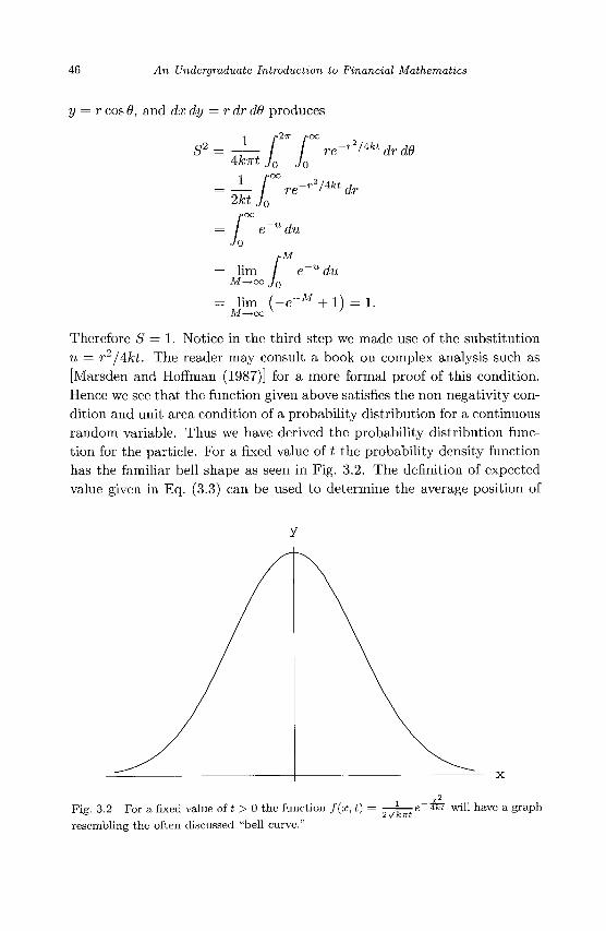
46 An Undergraduate Introduction to Financial Mathematics
y = r cos 8, and dxdy = r dr d6 produces
/•2-7T /'OO -i />Z7r re
™t J0 J0 ikirt -r2'Aktdrd6
L f° 2kt
f Jo
lim M^oo
re -rViktdr
' du
M
du
= lim \—e M ^ o o v
-M 1 ) = 1 .
Therefore 5 = 1. Notice in the third step we made use of the substitution u = r2/4kt. The reader may consult a book on complex analysis such as [Marsden and Hoffman (1987)] for a more formal proof of this condition. Hence we see that the function given above satisfies the non-negativity condition and unit area condition of a probability distribution for a continuous random variable. Thus we have derived the probability distribution function for the particle. For a fixed value of t the probability density function has the familiar bell shape as seen in Fig. 3.2. The definition of expected value given in Eq. (3.3) can be used to determine the average position of
Fig. 3.2 For a fixed value of t > 0 the function f(x, t)
resembling the often discussed "bell curve."
= e 4fct will have a graph
Normal Random Variables and Probability 47
the particle.
E[X]= / J — c
im /
2Vk7Tt M
-e 4kt dx
lim M
X
o 2vknt
kir
-e 4fct dx + lim N^oo J_N 2\/k-Kt
"**« dx
= lim W — ( l - e - M / 4 f e t
M-+00 V i
0
1 + lim \ — (e -N2/4kt
Thus, as might be expected, the average location of the particle is at the origin independent of t. This is due to the assumption that the particle has no preference for movement to the left or right. In a similar manner we may determine the variance of the position of the particle.
Var (X) X e-^dx-(E[X})2
— CO ^ V njTTb
L= lim f M
'knt
1
x2e ikt dx
'knt M^OO
1
lim 2kt Me~M 2 /4 f c t M
0
cM
2'iktdx
Vknt M^oc
2kt
ykirt Jo
2kt-
lim 2kt{Me~M2likt- f e^'^dx
e-*2/4fct dx
2Vknt J--^/Akt d x
2kt
We were able to avoid evaluating the last improper integral by making use of the unit area property of the probability distribution. From the derivation that a2 = 2kt we know that the "spread" in the location of the particle increases with time. This can be readily seen in the surface plot shown in Fig. 3.3.
If the particle were initially placed at location /i but all other assumptions remained the same then the probability distribution would simply be shifted in the x direction by ji. Thus we may define the normal proba-
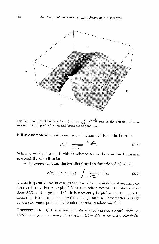
48 An Undergraduate Introduction to Financial Mathematics
f
Fig. 3.3 For t > 0 the function f(x,t) = 2Vk-rrt
section, but the profile flattens and broadens as t increases. retains the bell-shaped cross
bility distribution with mean /j, and variance a2 to be the function
1 _ ( * - M ) 2 m o-Jlix
(3.8)
When fj, = 0 and a = 1, this is referred to as the standard normal probability distribution.
In the sequel the cumulative distribution function <f>(x) where
P (X < x) 1 12-K
^ dt (3.9)
will be frequently used in discussions involving probabilities of normal random variables. For example if X is a standard normal random variable then P (X < 0) = 0(0) = 1/2. It is frequently helpful when dealing with normally distributed random variables to perform a mathematical change of variable which produces a standard normal random variable.
Theorem 3.6 If X is a normally distributed random variable with expected value ii and variance a2, then Z = (X-n)/a is normally distributed
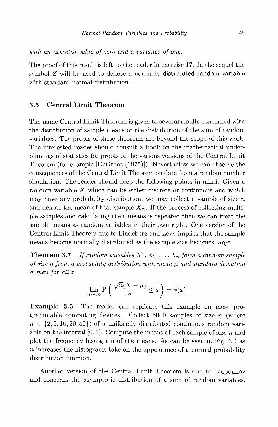
Normal Random Variables and Probability 49
with an expected value of zero and a variance of one.
The proof of this result is left to the reader in exercise 17. In the sequel the symbol Z will be used to denote a normally distributed random variable with standard normal distribution.
3.5 Central Limit Theorem
The name Central Limit Theorem is given to several results concerned with the distribution of sample means or the distribution of the sum of random variables. The proofs of these theorems are beyond the scope of this work. The interested reader should consult a book on the mathematical underpinnings of statistics for proofs of the various versions of the Central Limit Theorem (for example [DeGroot (1975)]). Nevertheless we can observe the consequences of the Central Limit Theorem on data from a random number simulation. The reader should keep the following points in mind. Given a random variable X which can be either discrete or continuous and which may have any probability distribution, we may collect a sample of size n and denote the mean of that sample Xn. If the process of collecting multiple samples and calculating their means is repeated then we can treat the sample means as random variables in their own right. One version of the Central Limit Theorem due to Lindeberg and Levy implies that the sample means become normally distributed as the sample size becomes large.
Theorem 3.7 If random variables X\, X2, • • •, Xn form a random sample of size n from a probability distribution with mean \i and standard deviation a then for all x
n—»oo \ a J
Example 3.5 The reader can replicate this example on most programmable computing devices. Collect 5000 samples of size n (where n € {2,5,10,20,40}) of a uniformly distributed continuous random variable on the interval [0,1]. Compute the means of each sample of size n and plot the frequency histogram of the means. As can be seen in Fig. 3.4 as n increases the histograms take on the appearance of a normal probability distribution function.
Another version of the Central Limit Theorem is due to Liapounov and concerns the asymptotic distribution of a sum of random variables.
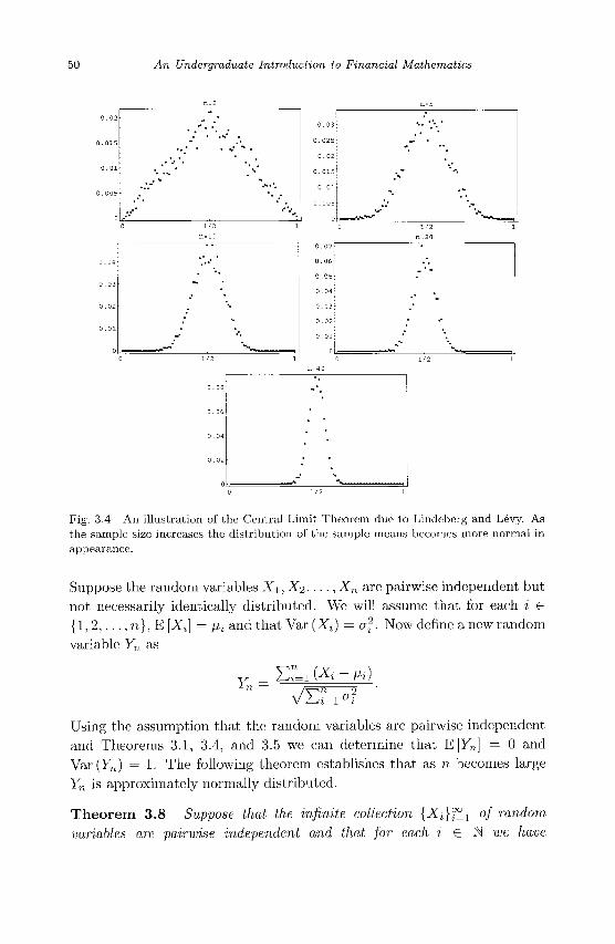
50 An Undergraduate Introduction to Financial Mathematics
0.03
0.025
0.02
0.015
0.01
0.005
0 .t
..
„
\"
n=5
- •
•'• .-•„
' • w
0.07
0. 06
0.05
0.04
0.03
0.02
0.01
0
0
H
1
n=
-
/2
20
" **
-
1
Fig. 3.4 An illustration of the Central Limit Theorem due to Lindeberg and Levy. As the sample size increases the distribution of the sample means becomes more normal in appearance.
Suppose the random variables X\, X2, • • ., Xn are pairwise independent but not necessarily identically distributed. We will assume that for each i G {1 ,2 , . . . , n}, E [Xi] = [ii and that Var (JQ) = of. Now define a new random variable Y„ as
Yn EILi {xt m
VEr=i ai Using the assumption that the random variables are pairwise independent and Theorems 3.1, 3.4, and 3.5 we can determine that E [Yn] = 0 and Var(F„) = 1. The following theorem establishes that as n becomes large Yn is approximately normally distributed.
Theorem 3.8 Suppose that the infinite collection {Xi}^ of random variables are pairwise independent and that for each i G N we have
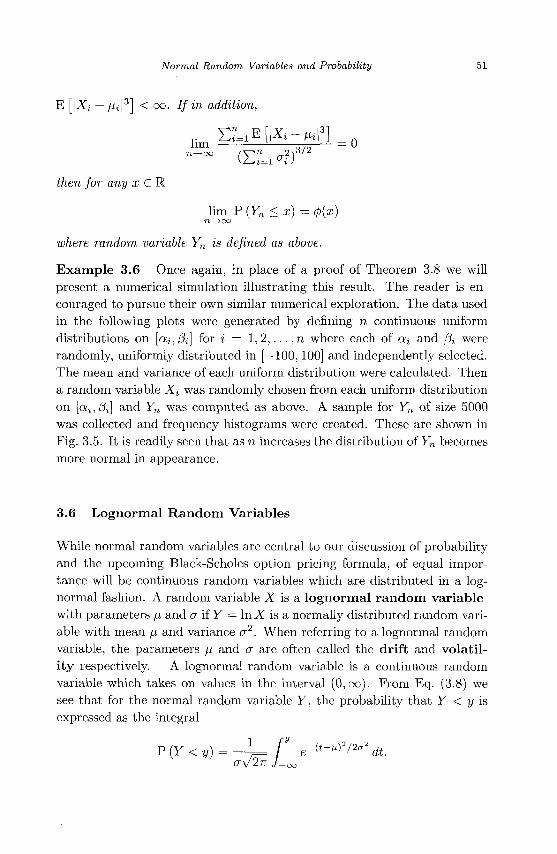
Normal Random Variables and Probability 51
E [\Xi — Hi\3] < oo. / / in addition,
then for any i £ l
lim P (Yn <x)= <p{x) n—>oo
where random variable Yn is defined as above.
Example 3.6 Once again, in place of a proof of Theorem 3.8 we will present a numerical simulation illustrating this result. The reader is encouraged to pursue their own similar numerical exploration. The data used in the following plots were generated by defining n continuous uniform distributions on [ai,/3,] for i = 1,2, . . . , n where each of on and /3j were randomly, uniformly distributed in [—100,100] and independently selected. The mean and variance of each uniform distribution were calculated. Then a random variable Xi was randomly chosen from each uniform distribution on [ai,j3i] and Yn was computed as above. A sample for Yn of size 5000 was collected and frequency histograms were created. These are shown in Fig. 3.5. It is readily seen that as n increases the distribution of Yn becomes more normal in appearance.
3.6 Lognormal Random Variables
While normal random variables are central to our discussion of probability and the upcoming Black-Scholes option pricing formula, of equal importance will be continuous random variables which are distributed in a log-normal fashion. A random variable X is a lognormal random variable with parameters (j, and a if Y = In X is a normally distributed random variable with mean fj, and variance a2. When referring to a lognormal random variable, the parameters [i and a are often called the drift and volatility respectively. A lognormal random variable is a continuous random variable which takes on values in the interval (0, oo). From Eq. (3.8) we see that for the normal random variable Y, the probability that Y < y is expressed as the integral
p (Y < y)=-i= r e-(*-")2/2^ dL o-\/27r J-oo
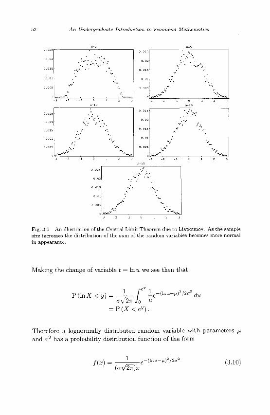
52 An Undergraduate Introduction to Financial Mathematics
0.025
0.02
0 .015
0 . 0 1
0 .005
- 3
-•*
- 2
• - • '
-''
- 1
V
—*
n 0
= 20
. " • ' > ;
i 2 3
- 1 0 1 2 3 - 3 - 2 - 1 0 1 2 3 n=50
0 .025
0 .02
0 .015
0 . 0 1
0 .005
0 _.V*~
\
.'-V
»•
•v • s .
.•••" •s - 3 - 2 - 1 0 1 2 3
Fig. 3.5 An illustration of the Central Limit Theorem due to Liapounov. As the sample size increases the distribution of the sum of the random variables becomes more normal in appearance.
Making the change of variable t = In u we see then that
P ( l n X < 2 / ) CTV^ Jo u
P (X < ey).
-(\nu-fj,)2/2a2 ^u
Therefore a lognormally distributed random variable with parameters fi and a2 has a probability distribution function of the form
/(*) 1
(<JV2-K)X (3.10)
Normal Random Variables and Probability 53
for 0 < x < oo. The probability that the lognormally distributed random variable X is less than y > 0 is then
P (X < y) = - 4 = f ie- '1"*-")2 /^ dx = d>(]ny), (3.11) (TV 2lT JO X
where <p(x) is the cumulative probability distribution function for a normal random variable with mean zero and variance one. Similarly the P (X > y) = 1 — (/>(ln y) for a lognormally distributed random variable.
Using the definitions of expected value and variance we can prove the following lemma.
Lemma 3.1 If X is a lognormal random variable with parameters /J, and a then
E[X] = e^+CT2/2 (3.12)
Var (X) = e2"+ff2 ( > ' - l ) (3.13)
Proof. Since X is assumed to be lognormal, then Y = In X is normally distributed with E [Y] = \i and Var (Y) = a2. By Eq. (3.3)
= e M+<r 2 /2
The last equality is true since the integral represents the area under the probability distribution curve for a normal random variable with mean l-i + a2 and variance a2.
54 An Undergraduate Introduction to Financial Mathematics
Likewise by Eq. (3.5)
Var (X) = E [X2] - (E[X]f
D2i/p-te-M)2/2cT2 dy _ feu.+a2/2Y i r
e "e
1 ' e~(y-(fJ.+2a)y/2e2(p.+a2)dy_e2li+a2
ay/2TV J-
2(n+a') x / „ - ( ! / - (^+2 t 7)) 2 /2 J „ _ „2M+a
e2(^+o-2) _ g2M+o-2
oo
dy-e
e 2M+^ ( ^ - . ) D
Now we will apply the concept of the lognormally distributed random variable to the situation of the price of a stock or other security. Suppose that the selling price of a security will be measured daily and that the starting measurement will be denoted S(0). For n > 1, we will let S(n) denote the selling price on day n. To a good approximation the ratios of consecutive days' selling prices are lognormal random variables, i.e. the expressions X(n) = S(n)/S(n — 1) for n > 1 are lognormally distributed. It is also generally assumed that the ratios are independent. If a sufficient number of measurements have been made that a financial analyst estimates the parameters of the random variable X are [i = 0.0155 and a = 0.0750, then questions regarding the likelihood of future prices of the security can be answered.
Example 3.7 First, what is the probability that the selling price of the stock on the next day will be higher than the price on the present day?
P p i T ( n ) > l ) = P( lnX(n) > 0)
a
= P(z> -0.206667)
= 1 - ^(-0.206667)
« 0.581865
Thus for a security with the parameters measured and reported above, there is a better than one half probability of the selling price increasing on any given day.
Normal Random Variables and Probability 55
Second, we may ask what is the probability that the selling price two days hence will be higher than the present selling price? At first glance the reader may be tempted to use the fact that each observation of the random variable is independent and hence declare that the sought after probability is 0.5622 ss 0.316. This implies the mistaken assumption that the price of the security increased on each of the two days. This ignores the possibility that the price of the security could decrease on either (but not both) of the two days and still make a net gain over the two-day period. To correctly approach the problem we must make use of the Central Limit Theorem.
P ( S ( B + S ) / S ( B ) > 1 ) . P ( ^ M > 1
= P ( ( X ( n ) ) 2 > l )
= P(21nX(n) > 0 )
_ r / , 0 -2(0 .0155) \
V 0.0750\/2 J
= P(z> -0.292271)
= l-<£(-0.292271)
« 0.61496
Thus the probability of a gain over a two-day period is nearly twice as large as may have been first suspected.
The assumption that ratios of selling prices sampled at regular intervals for securities are lognormally distributed will be explored further in Chapter 5. Appendix A contains a sample of closing prices for Sony Corporation stock. Readers can collect their own data set from many corporations' websites or from finance sites such as finaiice.yahoo.com. The eager reader may want to collect data for a particular stock to further test the lognormal hypothesis.
3.7 Properties of Expected Value
In later chapters the reader will encounter frequent references to the positive part of the difference of two quantities. For instance if an investor may purchase a security worth X for price K, then the excess profit (if any) of the transaction is the positive part of the difference X — K. This is typically denoted (X-K) + = max{0, X—K}. In this section a theorem and several corollaries are presented which will enable the reader to calculate
56 An Undergraduate Introduction to Financial Mathematics
the expected value of (X — K)+ when X is a continuous random variable and K is a constant.
Theorem 3.9 Let X be a continuous random variable with probability distribution function f{x). If K is a constant then
E [(X - K)+] = J (J°° f(t) dt) dx. (3.14)
Proof. For any x > 0, (X — K)+ > x \i and only if X — K > x, which is true if and only if X > K + x.
P ((X - K)+ >x)=l-P((X- K)+ < x)
= l-P(X<K + x) i-K+x
= 1- f(t)dt
J — CO
Therefore we have
rK+x E[{X-K)+]=J~(l-J_ f{t) dt dx
1 — / f(u) du 1 dx where u = t — K K
oo \
f(t)dt) dx. K
The last equality is true because f(x) is a probability distribution for the continuous random variable X. •
We can immediately put Theorem 3.9 to work finding the expected value of the positive part of a normal random variable. Corollary 3.1 is a special case of Theorem 3.9.
Corollary 3.1 If X is normal random variable with mean (j, and variance a2 and K is a constant, then
E \{X - K)+) = °-(»-K)2/^2 + fr - K)cf> (!±—£) • (3.15) V27T V cr J
Proof. By Theorem 3.9 the expected value of (X — K)+ is
/>oo -i />oo
E[{X-K)+]= -j=^ e-C-tf'^'dtdx JK V 27TCT Jx
Normal Random Variables and Probability 57
Employing integration by parts with
1 f°° u = -jL- / e~(*-M)2/2CT
2 dt v = x
\J2-Ka Jx
du = -L^e-(*-tf/*°* dv = dx, V27T0-
the expected value becomes
E[(X-K)+] K - f™ e-^2l^dt+ -L- r te-^l^dt
T JK V27rcr JK
/ e-z'2dz+-j= {az + n)e-<' /2 dz J-oo V 2-7T J(K-n)/a
_K4> f ^ E ) + - £ = / " e - 2 / 2 dz+-^=r ze^'2 dz \ a ) V27T J (K- M ) /CT V27T J(K-ti)/a
\ a J V \ °~ / / V27T J(K-iiy/2<r2
For the purpose of completing the mean-variance analysis encountered
later in Chapter 10 we must also be able to apply Theorem 3.9 when X is
a lognormally distributed random variable.
Corol lary 3.2 If X is a lognormally distributed random variable with
parameters \i and a2 and K > 0 is a constant then
E [{X - K)+] = e « + ^ ( ^ ± K + a ) - K<p ( ^ ^ ) (3-16)
Proof. According to Theorem 3.9
/•OO / /*00 \
E [(X - K)+] = J^ I J f(t) dt) dx
JK \V2^O-JX t t-rf/2a*dA dx
where the last equation is obtained using Eq. (3.10). Making the substitu
tion z — ( ln i — j-i)/o- allows us to write
E ax ~ K)+] = r (-±= r e z I2 dz\ dx
58 An Undergraduate Introduction to Financial Mathematics
This last integral will be evaluated using integration by parts with
V^TT J(\nx-~-*'<2dz u = nr— I e ' dz v = x
' (lnx—/x)/<x
du = _ ^ e - 0 n x - M ) 2 / 2 a 2 d x ^ = dx_
'2irax
Therefore we have
E[(X-K)+]
K r - V 2 ^ + 1 / e-0n,-,r/2^dx
\/27r J(lnK-n)/a V^TTa JK
\ o- J V2iraJinK
\ eM+^2/2 27TCT JlnK V O- J
^ 1 ^ (»-^K +a\-K<t> ( ^ K
U
3.8 Properties of Variance
In this section we will derive properties of the variance for the positive part of the difference of a continuous random variable and a constant. These results will be of use in later sections of this text.
Lemma 3.2 Let X be a normally distributed random variable with mean ji and variance a'. If K is a constant then
E[((X-K)+)2}
({p-2Kf + «>)t(^) + {-^^e-^. (3.17)
Normal Random Variables and Probability 59
Proof. Since X is normally distributed with mean \x and variance er2, then X — K is normally distributed with mean \i — K and variance a2.
E[((X-K)+)2}
^ ((X- K) + fe-^^-K)f/2^ dx
27R7 J-oo
^ / (x - Kfe-t*-i»-K)Yl^ dx 2na JK
1 Z"0 0
7 = / (at + /j,-2K)2e-t2/2dt '2n J(2K-u)/o l(2K~fi)/a
upon making the substitution t = (x — (/i — K))/a. Expanding the square in the last integrand and integrating produces
E[((X-K)+)2}
„ m 2 l (n-2K\ 2U-2K)a f°° , 2 / 2 ,
V °~ J \2-K J(2K-u)/cr
1, i2e-*2/2 dt 2-K J(2K-n)/<r
(/x _ 2 K ) ^ ( ^ _ ^ ) + _ _ _ _ e
( / / - 2 i Q < X c _ ( u _ 2 J 0 2 / 2 f f 2 ^ / / i - 2 A -
= ((/* - 2if)2 + a2) 0 ( ^ ^ ) + ( M - ^ ^ - ( ^ x ^ \ °~ J \/2TT D
Now the following result is immediately established.
Corollary 3.3 Lei X be a normally distributed random variable with mean fi and variance a2. If K is a constant then
Var ({X - K)+)
= ((/x - 2K)2 + a2) <p (0LZ2E\ + ^-^)\-^-2K)i,2„* \ & J V2TT
- ( ^ c - ^ - ^ W + ( / i _ K)4> ( ^ ) ) 2 - (3.18)
Now we must establish a similar result for lognormally distributed random variables.
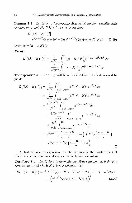
60 An Undergraduate Introduction to Financial Mathematics
Lemma 3.3 Let X be a lognormally distributed random variable with parameters fi and a2. If K > 0 is a constant then
E[((X-K)+f]
= e2^+a2)(f>{w + 2a) - 2Ke^+a2/2(j){w + a) + K2<t>{w) (3.19)
where w = (fj, — \nK)/a.
Proof.
E [((X - K)+)2} = -jL- / (( i - K)+f±e-Qnx-tf/2°a dx V 2iro~ Jo x
L- r \ x - Kf-e-^x~^''^ dx 2na JK %
The expression az = In x — \i will be substituted into the last integral to yield:
1 f°° E [{(X - K)+)2} = -±= / ( e C T ^ - K)2e-z2l2 dz
= - ± = / (e°z+»-K)2e-z2/2dz V2lT J(\nK-tJ.)/(T
„2(u+<rJ) 6 ' e-^2^'2dz
\/2lT J(\nK-tt)/.
2K^'°'2 r .-<->•*„, V2n J(\nK-ii)/(T
is1} r°° K f e-<*-°f*dz V2ir J (in K-u)/o
g 2 ( A t + C T ^ / M - l n ^ + 2 \+K2J»-\nK
2Ke^2'2Jll-lnK+ a a
At last we have an expression for the variance of the positive part of the difference of a lognormal random variable and a constant.
Corollary 3.4 Let X be a lognormally distributed random variable with parameters /i and a2. If K > 0 is a constant then
Var ((X - K)+) = e^^l<f>(w + 2a) - 2KeIJ'+'j2/2<j>(w + a) + K2(j>(w)
- (e^+(j2l2(j){w + a)- K<t>(w)^ (3.20)
Normal Random Variables and Probability 61
where w = (/x — hiK)/a.
3.9 Exercises
(1) Random variable X is continuously uniformly distributed in the interval [-4,1]. Find P (X > 0).
(2) Random variable X is continuously distributed on the interval (1, oo), with probability distribution function
/(*) -% if 1 < x 0 otherwise.
Determine the value of c. (3) Show using properties of the definite integral that for a continuous
random variable X with probability distribution function f(x),
P{X>a) = l-P(X<a).
(4) A random variable X has a continuous Cauchy distribution with probability density function
7r(l + XZ)
Show that the mean of this random variable does not exist. (5) If X is a continuous random variable with probability density function
f(x), show that E [aX + b] = aE [X] + b where a, b e R. (6) Prove Theorem 3.1. (7) Prove Theorem 3.2. (8) Prove Theorem 3.3. (9) Prove Theorem 3.4.
(10) Prove Theorem 3.5. (11) Find the expected value and variance of the continuous random vari
able X whose probability distribution function is given by
/(a;) = / ! N i f - 1 < ^ < 2 . \ 0 otherwise.
(12) Show that if m and n are integers then n — m is even if and only if n + m is even.
62 An Undergraduate Introduction to Financial Mathematics
(13) Evaluate the following indefinite integral.
(14) Use the technique of integration by parts to evaluate
(15) Evaluate the following limit with k > 0 and t > 0.
lim 2ktMe-M"'4kt
(16) Using a computer algebra system, graphing calculator, or some numerical method evaluate the following probabilities for a standard normal random variable:
(a) P ( - K X < 1) (b) P ( - 2 < X < 2 ) (c) P ( -3 < X < 3) (d) P ( K X < 3 )
(17) Prove Theorem 3.6. (18) The annual rainfall amount in a geographical area is normally dis
tributed with a mean of 14 inches and a standard deviation of 3.2 inches. What is the probability that the sum of the annual rainfalls in two consecutive years will exceed 30 inches?
(19) The ratio of selling prices of a security on consecutive days is a log-normally distributed random variable with parameters fi = 0.01 and a = 0.05. What the probability of a one-day increase in the selling price? What is the probability of a one-day decrease in the selling price? What is the probability of a four-day decrease in the selling price of the security?
(20) Let X be a uniformly distributed continuous random variable on the interval [a, b]. If K is a constant, find an expression for E \{X — K)+}.
(21) Show that for the standard normal random variable \ — <j>(x) — <fi(—x). (22) Fill in the details of the proof of Corollary 3.3. (23) Fill in the details of the proof of Corollary 3.4.
Chapter 4
The Arbitrage Theorem
The concept known as arbitrage is subtle and can seem counter-intuitive. In its basic form arbitrage exists whenever two financial instruments are mis-priced relative to one another. Due to the mis-pricing, it becomes possible to make a financial gain. For example suppose bank A issues loans at a 5% interest rate and bank B offers a savings account which pays 6% interest. A person could take out a loan from bank A and place the loan into savings with bank B. When it becomes time to repay bank A for the loan, the person closes the savings account with bank B, repays the principal and interest and still has 1% of the loaned amount as profit. The assumption that financial markets are efficient prevents such obvious arbitrage opportunities from being commonplace. When arbitrage opportunities arise, investors wanting to make a profit flock to the mis-priced instruments and the financial market reacts by correcting the pricing of the instruments.
We will see that financial instruments such as options, bonds, and stocks must be priced so as to be "arbitrage free." It is this absence of arbitrage which forms the basis of the derivation of the Black-Scholes equation found in Chapter 6.
4.1 The Concept of Arbitrage
As mentioned previously one way to think about arbitrage is as the situation which arises when two financial instruments are mis-priced relative to one another. In this section we will refine and make precise our definition. Suppose there is a set of possible outcomes for some experiment and that wagers can be placed on those outcomes. The Arbitrage Theorem states that either the probabilities of the outcomes are such that all bets are fair, or there is a betting scheme which produces a positive gain independent
63
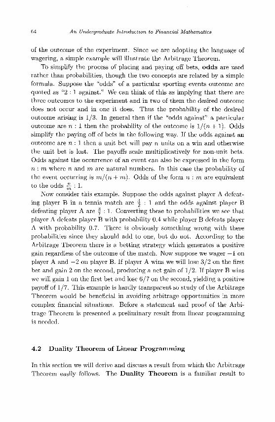
64 An Undergraduate Introduction to Financial Mathematics
of the outcome of the experiment. Since we are adopting the language of wagering, a simple example will illustrate the Arbitrage Theorem.
To simplify the process of placing and paying off bets, odds are used rather than probabilities, though the two concepts are related by a simple formula. Suppose the "odds" of a particular sporting events outcome are quoted as "2 : 1 against." We can think of this as implying that there are three outcomes to the experiment and in two of them the desired outcome does not occur and in one it does. Thus the probability of the desired outcome arising is 1/3. In general then if the "odds against" a particular outcome are n : 1 then the probability of the outcome is l / (n + 1). Odds simplify the paying off of bets in the following way. If the odds against an outcome are n : 1 then a unit bet will pay n units on a win and otherwise the unit bet is lost. The payoffs scale multiplicatively for non-unit bets. Odds against the occurrence of an event can also be expressed in the form n : m where n and m are natural numbers. In this case the probability of the event occurring is m/(n + m). Odds of the form n : m are equivalent to the odds ^ : 1.
Now consider this example. Suppose the odds against player A defeating player B in a tennis match are | : 1 and the odds against player B defeating player A are | : 1. Converting these to probabilities we see that player A defeats player B with probability 0.4 while player B defeats player A with probability 0.7. There is obviously something wrong with these probabilities since they should add to one, but do not. According to the Arbitrage Theorem there is a betting strategy which generates a positive gain regardless of the outcome of the match. Now suppose we wager —1 on player A and —2 on player B. If player A wins we will lose 3/2 on the first bet and gain 2 on the second, producing a net gain of 1/2. If player B wins we will gain 1 on the first bet and lose 6/7 on the second, yielding a positive payoff of 1/7. This example is hardly transparent so study of the Arbitrage Theorem would be beneficial in avoiding arbitrage opportunities in more complex financial situations. Before a statement and proof of the Arbitrage Theorem is presented a preliminary result from linear programming is needed.
4.2 Duality Theorem of Linear Programming
In this section we will derive and discuss a result from which the Arbitrage Theorem easily follows. The Duality Theorem is a familiar result to
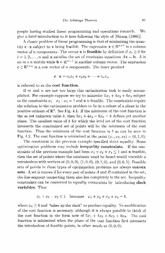
The Arbitrage Theorem 65
people having studied linear programming and operations research. We give a brief introduction to it here following the style of [Strang (1986)].
A classic problem of linear programming is that of minimizing the quantity c • x subject to x being feasible. The expression x 6 R n x l is a column vector of n components. The vector x is feasible by definition if X{ > 0 for i = 1,2,.. . , n and x satisfies the set of constraint equations Ax = b. A is an m x n matrix while b £ R m X l is another column vector. The expression c 6 M l x n is a row vector of n components. The inner product
C • X = C\X\ + C2X2 H h CnXn
is referred to as the cost function. If m and n are not too large this optimization task is easily accom
plished. For example suppose we try to minimize 5x\ + 4x2 + 8x3 subject to the constraints x\ + x2 +X3 = 1 and x is feasible. The constraints require the solution to the optimization problem to lie in a subset of a plane in the positive orthant of M3. See Fig. 4.1. If the minimum of the cost function is the as yet unknown value k, then 5x\ + Ax2 + 8x3 = k defines yet another plane. The smallest value of k for which the level set of the cost function intersects the constrained set of points will be the minimum of the cost function. Thus the minimum of the cost function is 4 as can be seen in Fig. 4.2. The cost function is minimized at the point (xi, x2, X3) = (0,1, 0).
The constraint in the previous example specified strict equality. Some optimization problems may include inequality constraints. If the constraints of the previous example had been x\ + x2 + X3 < 1 and x feasible, then the set of points where the minimum must be found would resemble a tetrahedron with vertices at (0,0, 0), (1,0,0), (0,1,0), and (0,0,1). Feasible sets of points in these types of optimization problems are always convex sets. A set is convex if for every pair of points A and B contained in the set, the line segment connecting them also lies completely in the set. Inequality constraints can be converted to equality constraints by introducing slack variables. Thus
x\ + x2 + x3 < 1 becomes x\ + x2 + x3 + X4 = 1,
where X4 > 0 and "takes up the slack" to produce equality. No modification of the cost function is necessary, although it is always possible to think of the cost function in the form now of 5a; 1 + 4x2 + 8x3 + OX4. The cost function is minimized when the plane of the cost function first intersects the tetrahedron of feasible points, in other words at (0,0, 0).
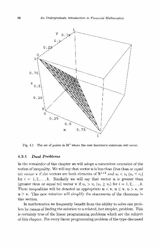
66 An Undergraduate Introduction to Financial Mathematics
Fig. 4.1 The set of points in R 3 where the cost function's minimum will occur.
4.2.1 Dual Problems
In the remainder of this chapter we will adopt a convenient extension of the notion of inequality. We will say that vector u is less than (less than or equal to) vector v if the vectors are both elements of Mlxfc and w, < Vi (u» < Vi) for i = 1,2, . . . ,&. Similarly we will say that vector u is greater than (greater than or equal to) vector v if Ui > v\ (itj > Vi) for i = 1, 2 , . . . , k. These inequalities will be denoted as appropriate u < v , u < v , u > v , or u > v. This new notation will simplify the statements of the theorems in this section.
In mathematics we frequently benefit from the ability to solve one problem by means of finding the solution to a related, but simpler, problem. This is certainly true of the linear programming problems which are the subject of this chapter. For every linear programming problem of the type discussed
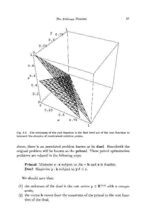
The Arbitrage Theorem 67
Fig. 4.2 The minimum of the cost function is the first level set of the cost function to intersect the simplex of constrained solution points.
above, there is an associated problem known as its dual. Henceforth the original problem will be known as the primal. These paired optimization problems are related in the following ways.
Primal: Minimize c • x subject to Ax. = b and x is feasible. Dual: Maximize y • b subject to yA < c.
We should note that:
(1) the unknown of the dual is the row vector y £ Klx™ with n components,
(2) the vector b moves from the constraint of the primal to the cost function of the dual,
68 An Undergraduate Introduction to Financial Mathematics
(3) the vector c moves from the cost of the primal to the constraint of the dual,
(4) the constraints of the dual are inequalities and there are n of them, (5) there is no feasibility constraint (i.e. no y > 0) in the dual.
Given a primal or a dual problem it is a routine matter to construct its partner. Perhaps it is no surprise then that the solutions to the primal and dual are related.
Theorem 4.1 (Weak Duality Theorem) 7/x andy are the unknowns of the primal and dual problems respectively, then y-b < e x . 7 / y b = e x then these vectors are optimal for their respective problems.
Proof. Solutions to the primal and the dual problems must satisfy the constraints Ax. = b, xi > 0 for i = 1 , . . . , n and yA < c. We multiply the constraint in the primal by y and the constraint in the dual by x to obtain
y^4x = y • b and yAx < c • x.
The non-negativity of the components of x implied by the feasibility assumption on x preserve the inequality in the latter case. Therefore we have y • b = yAx < c • x or naturally y • b < c • x. If y • b = c • x then y and x must be optimal since no y can make y • b larger than c • x and no x can make c • x smaller than y • b. •
Example 4.1 Consider the paired primal and dual problems:
Primal: Minimize 4xi + 3^2 subject to x\ + x-i = 2 and Xi,x% > 0. Dual: Maximize yi subject to yi < 3 and 2/2 < 4.
While both problems may seem simple, the dual is trivial. The maximum value of 2/2 subject to the constraints must be 2/2 = 3 . According to the Weak Duality Theorem then the minimum of the cost function of the primal must be at least 3. Applying the level set argument as before, the smallest value of k for which Axi + 3^2 = k intersects the set of constrained, feasible points for the primal is k = 6. See Fig. 4.3.
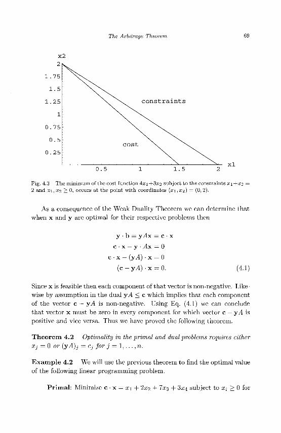
The Arbitrage Theorem 69
c o n s t r a i n t s
0 . 5 x l
Fig. 4.3 The minimum of the cost function Ax\ +3x2 subject to the constraints xi +x% = 2 and x\,X2 > 0, occurs at the point with coordinates (x±,X2) = (0,2).
As a consequence of the Weak Duality Theorem we can determine that when x and y are optimal for their respective problems then
y • b = yAx. = c • x
c • x — y • Ax = 0
c • x - (yA) • x = 0
(c - yA) • x = 0. (4.1)
Since x is feasible then each component of that vector is non-negative. Likewise by assumption in the dual yA < c which implies that each component of the vector c — yA is non-negative. Using Eq. (4.1) we can conclude that vector x must be zero in every component for which vector c — yA is positive and vice versa. Thus we have proved the following theorem.
Theorem 4.2 Optimality in the primal and dual problems requires either
Xj = 0 or (yA)j = Cj for j = 1 , . . . , n.
Example 4.2 We will use the previous theorem to find the optimal value of the following linear programming problem.
Primal: Minimize c • x = x\ + 2x2 + 7rc3 + 3^4 subject to Xi > 0 for

70 An Undergraduate Introduction to Financial Mathematics
i = 1,2,3,4 and
Xi
" 1 1 - 1 0 ' - 2 0 1 1
X2
%3 =
"5" 3
X4
Readers unfamiliar with matrix notation may wish to re-write Eq. (4.2) as a system of two linear equations with four unknowns. Since the set of points described by the constraints exists in four-dimensional space, it will be more difficult to use geometrical and graphical thinking to analyze this problem. Fortunately we can also analyze this problem's associated dual problem. Dual: Maximize y • b = 5j/i + 3j/2 subject to
< [12 7 3] (4.3)
The space of points on which the dual is to be optimized exists in two-dimensional space and thus is easily pictured. The constraints of the dual can be thought of as a system of inequalities.
2/i - 2y2 < 1
Vi < 2
-Vi + 2/2 < 7
2/2 < 3
This solution to this set of inequalities can be pictured as the shaded region shown in Fig. 4.4. The maximum of the cost function for the dual occurs at the point with coordinates (2/1,2/2) = (2,3). Thus the maximum value is 19 which will also be the minimum value of the primal problem's cost function. At the optimal point for the dual problem, strict inequality is present in the first and third constraints since
2 - 2(3) = - 4 < 3
- 2 + 3 = 1 < 7.
By the previous theorem then the first and third components of x in the primal problem must be zero. Therefore the primal can be recast as
[2/1 2/2: 1 1 - 1 0
- 2 0 1 1
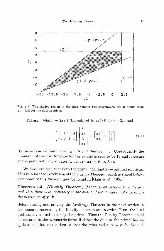
The Arbitrage Theorem 71
-y l+y2=7
y2=3 X
y l = 2-
, ^ T . I , , . .
- 1 5 - 1 2 . 5 - 1 0 - 7 . 5 - 5 - 2 . 5 0 2 . 5
y i
Fig. 4.4 The shaded region in the plot denotes the constrained set of points from Eq. (4.3) for the dual problem.
Primal: Minimize 2^2 + 3^4 subject to X{ > 0 for i = 2, 4 and
" 1 1 - 1 0 - 2 0 1 1
By inspection we must have x^ — 5 and thus X4 = 3. Consequently the minimum of the cost function for the primal is seen to be 19 and it occurs at the point with coordinates (xi,X2,X3,X4) = (0,5,0,3).
We have assumed that both the primal and dual have optimal solutions. This is in fact the conclusion of the Duality Theorem, which is stated below. The proof of this theorem may be found in [Gale et al. (1951)].
Theorem 4.3 (Duality Theorem) If there is an optimal x in the primal, then there is an optimal y in the dual and the minimum of c • x equals the maximum ofy-h.
Before stating and proving the Arbitrage Theorem in the next section, a few remarks concerning the Duality Theorem are in order. First, the dual problem has a dual - namely the primal. Thus the Duality Theorem could be restated in the symmetric form: if either the dual or the primal has an optimal solution vector then so does the other and c • x = y • b. Second,
6
4
2
- 2
- 4
- 6
0 X2
0 X4
= X2
X4 =
5 3
(4.4)
72 An Undergraduate Introduction to Financial Mathematics
if the primal has an inequality constraint Ax > b in place of the equality constraint Ax = b, then the dual possesses the extra constraint y > 0. To see this imagine introducing the slack variables xs in the primal. The primal in matrix form now resembles
[A-I]\*]=h . s .
while the dual becomes
y[A-l] < [ c 0 ] .
This implies the two vector inequalities yA < c and —y < 0. This last inequality is equivalent to y > 0. In conclusion the symmetric form the primal/dual pair can be stated as follows.
Primal: Minimize c • x subject to Ax > b and x > 0. Dual: Maximize y • b subject to yA < c and y > 0.
4.3 The Fundamental Theorem of Finance
Consider an experiment with m possible outcomes numbered 1 through m. Suppose we can place n wagers (numbered 1 through n) on the outcomes of the experiment. Let r^ be the return for a unit bet on wager i when the outcome of the experiment is j . The vector x = (x\,X2,--.,xn) is called a betting strategy. Component Xi is the amount placed on wager i. The composite return from a betting strategy is then Y^=i xi'rij- The Arbitrage Theorem states that the probabilities of the m outcomes of the experiment are such that the expected value of the payoff is zero, or there exists a betting strategy for which the payoff is positive regardless of the outcome of the experiment.
Theorem 4.4 (Arbitrage Theorem) Exactly one of the following is true: either
(1) there is a vector of probabilities y = (2/1,3/2, •• • ,Vm) for which
m
^2yjnj=0, for i = 1,2,..., n, or
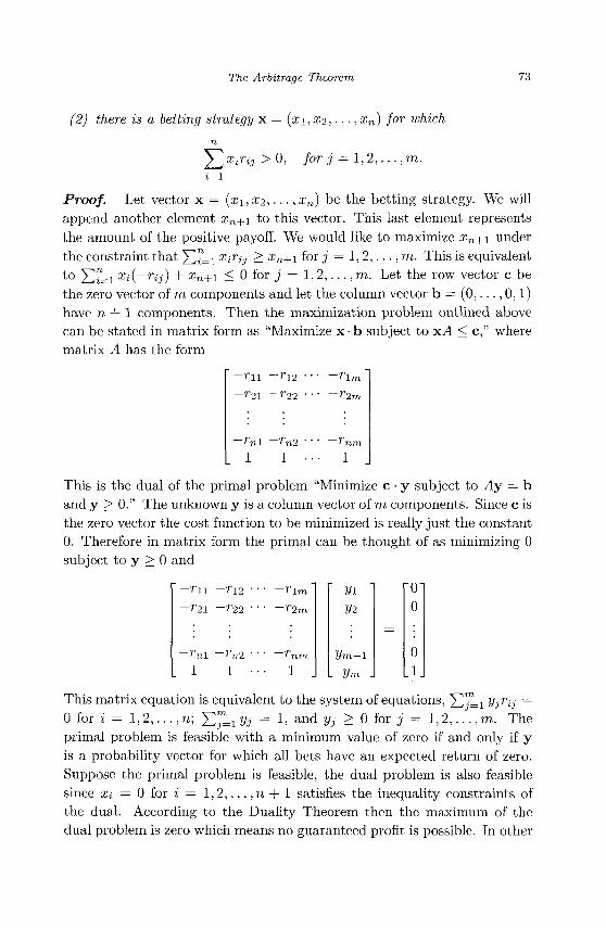
The Arbitrage Theorem 73
(2) there is a betting strategy x = (x\,X2, • • •, xn) for which
n
^2 x*rij > °> for j = 1,2,...,m.
Proof. Let vector x = (x\,X2, • • • ,xn) be the betting strategy. We will append another element xn+i to this vector. This last element represents the amount of the positive payoff. We would like to maximize xn+\ under the constraint that Y17=i xirij — xn+i for j = 1,2,... ,m. This is equivalent to Y17=i xi(~rij) + xn+i < 0 for j = 1, 2,..., m. Let the row vector c be the zero vector of m components and let the column vector b = ( 0 , . . . , 0,1) have n + 1 components. Then the maximization problem outlined above can be stated in matrix form as "Maximize x • b subject to xA < c," where matrix A has the form
r n J-21
rni
-T-12 • '
- r 2 2 • •
~Tn2 • •
• - n
• - r 2
• - r n
1 1 1
This is the dual of the primal problem "Minimize c • y subject to Ay = b and y > 0." The unknown y is a column vector of m components. Since c is the zero vector the cost function to be minimized is really just the constant 0. Therefore in matrix form the primal can be thought of as minimizing 0 subject to y > 0 and
r u T21
rn\ 1
-rl2 .. - r 2 2 • •
-Tra • •
1 ••
• -rim'
• ~r2m
rnm
1
J/1
2/2
Z / m - 1
. Vm .
"0 0
0 .1
This matrix equation is equivalent to the system of equations, X^fci Virii =
0 for i = 1, 2 , . . . , n\ Y^j=i Vj = 1J a n ( i Vj > 0 iov j = 1,2,... ,m. The primal problem is feasible with a minimum value of zero if and only if y is a probability vector for which all bets have an expected return of zero. Suppose the primal problem is feasible, the dual problem is also feasible since xt = 0 for i = 1, 2,..., n + 1 satisfies the inequality constraints of the dual. According to the Duality Theorem then the maximum of the dual problem is zero which means no guaranteed profit is possible. In other
74 An Undergraduate Introduction to Financial Mathematics
words if (1) is true then (2) is false. Now suppose the primal problem is not feasible. According to the Duality Theorem the dual problem has no optimal solution. Therefore zero is not the maximum payoff, thus there is a betting strategy which produces a positive payoff. Thus we see that if (1) is false then (2) is true. •
4.4 Exercises
(1) Suppose the odds against the three possible outcomes of an experiment are as given in the table below.
Outcome A B C
Odds 2:1 3:1 1:1
Find a betting strategy which produces a positive net profit regardless of the outcome of the experiment.
(2) Sketch the region in the plane which satisfies the following inequalities:
x\ + 3x2 > 6
3x\ + X2 > 6
xi > 0
X2 > 0
Is the region convex? What are the coordinates of the points at the corners of the region?
(3) Minimize the cost function x\ +X2 on the region described in exercise 2. (4) Find inequality constraints which will describe the rectangular region
with corners at (0,0), (2,0), (2,3), and (0,3). (5) Introduce slack variables in the inequality constraints found in exer
cise 4 to produce equality constraints Ax = b . What are A and b? (6) Minimize the cost function x\ + X2 + 2x3 on the set where x\ + 2x2 +
3^3 = 15 and Xi > 0 for i = 1,2,3. (7) Minimize the cost function 7x2 + 9x3 subject to the constraints X\ +
X2 + %3 = 5 and X2 + 0:3 + 2x4 = 1 with Xi > 0. (8) Write down the dual problem of the following primal problem: Mini
mize xi + x2 + x3 subject to 2xi + x2 = 4 and X3 < 6 with Xj > 0.
The Arbitrage Theorem 75
(9) Find the solutions to the primal and dual problems of exercise 8. (10) Write down the primal companion problem to the dual problem: Max
imize 2yi + 4y3 subject to y\ - y2 < 1 and y2 + 2y3 < - 1 . (11) Find the solutions to the primal and dual problems of exercise 10.

This page is intentionally left blank
Chapter 5
Random Walks and Brownian Motion
In this chapter we will introduce and explain some of the concepts surrounding the probabilistic models used to capture the behavior of stock, security, option, and index prices. Topics covered here could be expanded into an entire book of their own. For our purposes we will explore just enough of the stochastic calculus to provide some justification for Ito's Lemma, the main result of this chapter.
5.1 Intuitive Idea of a Random Walk
Earlier in Chapter 3 we analyzed the motion of a particle taking a discrete step along the rr-axis during every "tick" of the clock. At first it was revealed that the location of the particle relative to the origin followed a binomial distribution. As the step size was decreased, the probability of the particle lying in a particular interval was seen to obey the normal distribution. In this chapter we will extend this discussion to a more general setting. Imagine a person standing at the origin of the real number line. They will flip a coin. For every time the coin lands on heads, they will take a unit step to the right (the positive direction). For every time the coin lands on tails, they will move a unit step to the left (the negative direction). The evolution of this stochastic discrete dynamical system is called a random walk. A plot of the person's location versus the number of times the coin has been flipped might resemble the graph in Fig. 5.1. Random walks do not require that the probabilities of moving left or right be equal (i.e. the coin does not have to be fair). The magnitude of the movement at each stage does not have to a single unit. The person could move left or right depending on the value of a random number chosen from a normal distribution for example. The bias in choosing to move left or right and the possibility of moving
77
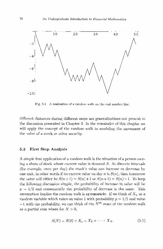
78 An Undergraduate Introduction to Financial Mathematics
Fig. 5.1 A realization of a random walk on the real number line.
different distances during different steps are generalizations not present in the discussion presented in Chapter 3. In the remainder of this chapter we will apply the concept of the random walk to modeling the movement of the value of a stock or other security.
5.2 First Step Analysis
A simple first application of a random walk is the situation of a person owning a share of stock whose current value is denoted S. At discrete intervals (for example, once per day) the stock's value can increase or decrease by one unit, in other words if its current value on day n is S(n), then tomorrow the value will either be S{n+1) = S(n) +1 or S(n+1) = S{n) -1. To keep the following discussion simple, the probability of increase in value will be p = 1/2 and consequently the probability of decrease is the same. This assumption implies the random walk is symmetric. If we think of Xn as a random variable which takes on value 1 with probability p = 1/2 and value — 1 with the probability, we can think of the Nth state of the random walk as a partial sum where for A" > 0,
S(N) = S(0) + X1+X2 + --- + XN. (5.1)
Random Walks and Brownian Motion 79
The random variable Xn is a generalization of the Bernoulli random variable discussed earlier. S(N) can be defined inductively by the formula S(N) = S(N—1)+XN for N > 0 where 5(0) is a specified initial state of the walk. If we assume that the random variables X, and Xj are identically distributed and independent for i ^ j then we see that the transitions between states in the random walk, S(N) — S(N—1) = XN are independent random variables. If the initial state of the random walk is 5(0) and n > 0 steps are taken, where k > 0 of the steps are in the positive direction and n — k > 0 are in the negative direction, then
P (S(ra) = 5(0) + k-(n-k)) = P (S(n) - 5(0) = 2k - n)
The last expression is the familiar probability formula for a binomial random variable with p = 1/2.
If 5(0) ^ 0 then we can perform a change of variable via T(n) = S(n) — 5(0) for n = 0 , 1 , . . . and define a related random walk where T(0) = 0. The transitions in the states of the new random walk are independent, identically distributed random variables just as before. Likewise we see that
P(T(n) = 2 f c - n ) = Q ( £ ) n . (5.2)
Thus without loss of generality we will assume that 5(0) = 0. Now that we have settled on a starting state for the random walk, what states can be visited in n steps? The next lemma provides the answer and the respective probabilities of reaching these states.
Lemma 5.1 For the random walk defined in Eq. (5.1) with initial state 5(0) = 0,
(1) P (S{n) = TO) = 0 if \m\ > n, (2) P (S{n) = m) = 0ifn + mis odd, (3) P(5(n) = TO) = ({n+
nm)/2) (\)n, otherwise .
Proof.
(1) According to Eq. (5.1), —n < S(n) < n, thus if \m\ > n the partial sum cannot attain this value.
(2) If we let TO = Ik - n in Eq. (5.2) then n + m = 2k which implies n + TO is even, contradicting the assumption that n + m i s odd.
80 An Undergraduate Introduction to Financial Mathematics
(3) We may assume that n + m is even and thus the result is shown by Eq. (5.2). Q
In the previous discussion the random walk was free to move in either the positive or negative direction any integer amount as the number of steps increased. Suppose that bounds are placed in the path the particle may follow. Once again, for the sake of simplicity, we will assume the initial state of the random walk is positive, i.e. S(0) > 0 and we will assume the random walk has a lower boundary of 0. If the state of the random walk reaches the lower boundary in a finite number of steps then the state remains at that boundary value. In the study of random walks, this is known as an absorbing boundary condition. In a financial setting we may think of the value of a security as following a random walk (though in reality a much more complicated one than the type we are exploring here). If the value of the security drops to 0, the security becomes worthless to the owner. We must further generalize our discussion of random walks to include the absorbing boundary. There are two questions related to this situation that we wish to explore.
(1) What is the probability that the state of the random walk crosses a threshold value of A > 0 before it hits the boundary at 0 (and hence remains there)?
(2) What is the expected value of the number of steps which will elapse before the state of the random variable first crosses the A > 0 threshold?
Figure 5.2 shows a random walk of a stock whose value was initially 10. This situation has been so simplified and abstracted from the reality of the stock market that it is of little use in making investment decisions, but serves as an instructive example of the use of the concept of a random walk. The answers to the two primary questions will be found following the lines of reasoning laid out in [Kijima (2003)] and [Steele (2001)].
Since the boundary at 0 is absorbing we must keep track of the smallest value which S(n) takes on. Thus we define m„ = mm{S(k) : 0 < k < n}. If i is the smallest non-negative integer such that rrii = 0 (and hence that S(i) = 0) then by the absorbing boundary condition S(k) = 0 for all k > i. Our attention is now focused on developing an understanding of the following conditional probability:
p (S{n) = A A m„ > 0 | S(0) = i).
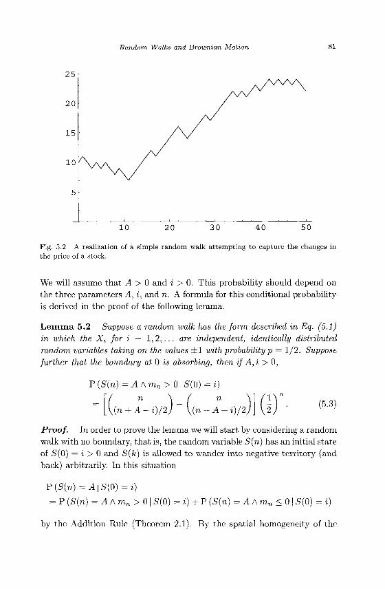
Random Walks and Brownian Motion 81
25
20
1 5
1 0
1 0 20 30 40 50
Fig. 5.2 A realization of a simple random walk attempting to capture the changes in the price of a stock.
We will assume that A > 0 and i > 0. This probability should depend on the three parameters A, i, and n. A formula for this conditional probability is derived in the proof of the following lemma.
Lemma 5.2 Suppose a random walk has the form described in Eq. (5.1) in which the Xj for i = 1,2,... are independent, identically distributed random variables taking on the values ±1 with probability p = 1/2. Suppose further that the boundary at 0 is absorbing, then if A,i > 0,
P (S(n) = A A m„ > 0 | S(0) = i)
\{n + A-i)/2) \{n- A-i)/2J _ (5.3)
Proof. In order to prove the lemma we will start by considering a random walk with no boundary, that is, the random variable S(n) has an initial state of S'(O) = i > 0 and S(k) is allowed to wander into negative territory (and back) arbitrarily. In this situation
P (S(n) = A | 5(0) = i)
= P (S(n) = A A m „ > 0 | 5(0) = i) + P (5(n) = A A mn < 0 | 5(0) = i)
by the Addition Rule (Theorem 2.1). By the spatial homogeneity of the
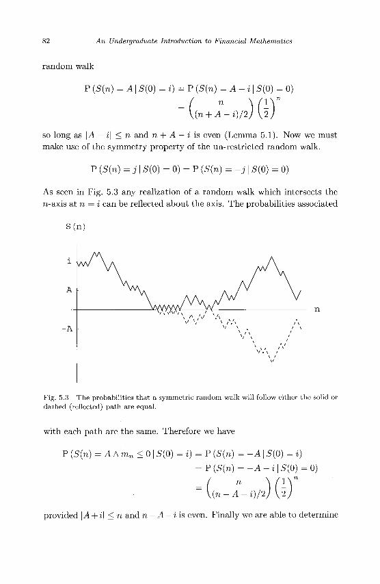
82 An Undergraduate Introduction to Financial Mathematics
random walk
P (5(n) = A | 5(0) = i) = P (5(n) =A-i\ 5(0) = 0)
{n + A-i)/2j U ,
so long as \A — i\ < n and n + A — i is even (Lemma 5.1). Now we must make use of the symmetry property of the un-restricted random walk.
P (S(n) = j | 5(0) = 0) = P (S(n) = -j | 5(0) = 0)
As seen in Fig. 5.3 any realization of a random walk which intersects the n-axis at n = i can be reflected about the axis. The probabilities associated
S(n)
n
Fig. 5.3 The probabilities that a symmetric random walk will follow either the solid or dashed (reflected) path are equal.
with each path are the same. Therefore we have
P (S(n) = A A mn < 0 | 5(0) = i) = P (S{n) = -A \ 5(0) = i)
= P(S(n) = -A-i\S(0) = 0)
n \(V "
,(n-A-i)/2j \2.
provided |A + i| < n and n — A — i is even. Finally we are able to determine
Random Walks and Brownian Motion 83
that
P (S(n) = i A m n > 0 | 5(0) = i) n )(-X-(
K{n + A-i)/2J \2j \(n
which is equivalent to the expression in Eq. (5.3)
n A-i)/2
• The previous theorem now provides an answer to the first of the two
questions posed.
Example 5.1 For a symmetric random walk with initial state £(0) = 10, what is the probability that £(50) = 16 and S{n) > 0 for n = 0 , 1 , . . . , 50?
Making use of the formula found in Eq. (5.3) we have
P (£(50) = 16 A TOSO > 0 | £(0) = 10) 50\ _ /50 28j 1,12
0.0787178.
-50
Since the current notation is so bulky, we will define the function
JAA71) (n-A-i)/2 \(n + A-i)/2/
and use it from now on. We will call the first time that the random walk £(n) equals A the
stopping time, denoted QA- The stopping time is a random variable. In the remainder of this section we will explore the probability that CI A takes on the various natural number values given the initial state of the random walk is £(0) = i > 0, parameter A > 0, and the boundary at 0 is absorbing. Suppose the initial state of the random walk £(0) = i > A > 0, then due to the spatial homogeneity of the random walk
P (£(n) = A A mn > A | £(0) =i) = P (£(n) = 0 A mn > 0 | £(0) =i-A).
f o = n if and only if S(n — 1) = 1, m„_i > 0 and Xn = —1. Therefore
P (n0 = n | £(0) =i-A)
= p (Xn = - 1 A S(n - 1) = 1 A m„_i > 0 | £(0) = i - A)
P (£(n - 1) = 1 A m n _i > 0 | £(0) = i - A)
fi,(i-A)(n- 1).
Consequently P (QA = n \ £(0) = i) = \fi^i-A){n — 1) as well.
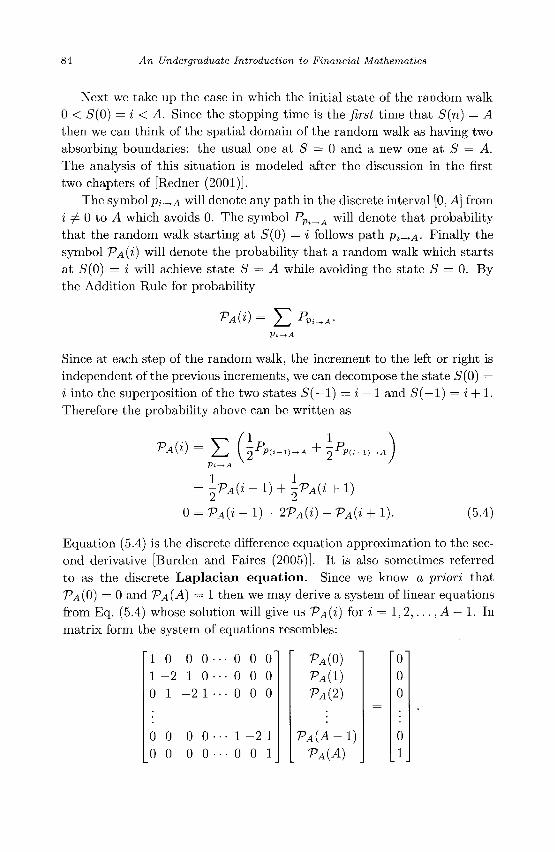
84 An Undergraduate Introduction to Financial Mathematics
Next we take up the case in which the initial state of the random walk 0 < 5(0) = i < A. Since the stopping time is the first time that S(n) = A then we can think of the spatial domain of the random walk as having two absorbing boundaries: the usual one at 5 = 0 and a new one at 5 = A. The analysis of this situation is modeled after the discussion in the first two chapters of [Redner (2001)].
The symbol Pi-^A will denote any path in the discrete interval [0, A] from i j^ 0 to A which avoids 0. The symbol PPi^A will denote that probability that the random walk starting at 5(0) = i follows path Pi->A- Finally the symbol VA{i) will denote the probability that a random walk which starts at 5(0) = i will achieve state 5 = A while avoiding the state 5 = 0. By the Addition Rule for probability
Since at each step of the random walk, the increment to the left or right is independent of the previous increments, we can decompose the state 5(0) = i into the superposition of the two states 5(—1) = i — 1 and 5(—1) = i + 1. Therefore the probability above can be written as
VA(i)= Y, f^.-.,,-, +=:Pv.
1
2 P(i-1)-+A ~ 2 P(i+1) —^
2VA(i-l) + f>A{i + l)
0 = VA{i - 1) - ZPA(i) + TA(i + 1). (5.4)
Equation (5.4) is the discrete difference equation approximation to the second derivative [Burden and Faires (2005)]. It is also sometimes referred to as the discrete Laplacian equation. Since we know a priori that PA (0) = 0 and VA (A) = 1 then we may derive a system of linear equations from Eq. (5.4) whose solution will give us VA{I) for i = 1,2,.. . , A — 1. In matrix form the system of equations resembles:
1 0 0 0-1 - 2 1 0 • 0 1 - 2 1-
0 0 0 0-0 0 0 0-
• 0 0 0 • 0 0 0 • 0 0 0
• 1 - 2 1 • 0 0 1
VA(0)
VA{1)
-PA{2)
VA(A-
PA(A)
Random Walks and Brownian Motion 85
The reader can verify that the solution to this matrix equation is
VA(0)
-PA(1)
rA(i)
PA(A-1)
VA(A)
=
0 1 A
i A
A-l A 1
By the symmetry of the random walk we also have
Po(0)
W)
^o(i)
Vo(A - 1) V0(A)
=
1
^
41
i 0
The expression Vo(i) is the probability that a symmetric random walk initially in state 5(0) = i achieves the state 5 = 0 while avoiding the state 5 = A. We can summarize these results in the following theorem.
Theorem 5.1 Suppose a random walk has the form described in Eq. (5.1) in which the Xj for i = 1,2,... are independent, identically distributed random variables taking on the values ±1 with probability p = 1/2. Suppose further that the boundaries at 0 and A are absorbing, then if 0 < 5(0) = i < A
(1) the probability that the random walk achieves state A without achieving state 0 is VA{i) = i/A,
(2) the probability that the random walk achieves state 0 without achieving state A is Vo(i) = 1 — i/A.
Before answering the question as to the expected stopping time for the random walk attaining state A, we will explore the simpler issue of the stopping time of reaching either of the two absorbing boundaries. Let B = {0, A} represent the discrete boundary set of the one-dimensional, discrete random walk. To help in the derivation we will define the following quantities:
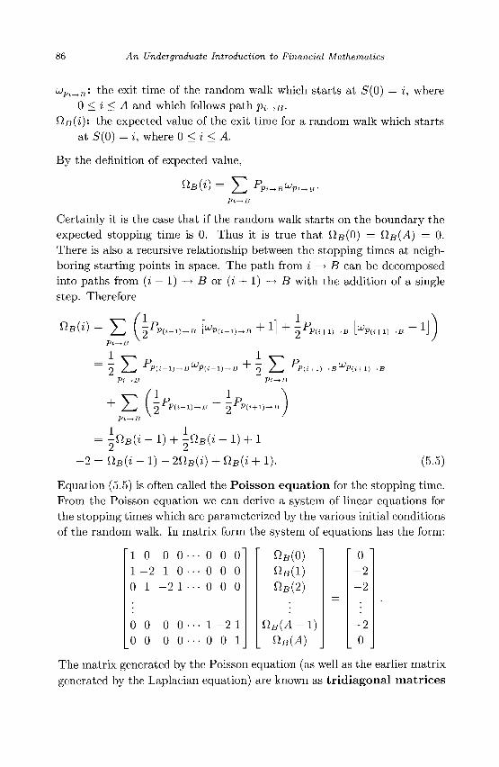
86 An Undergraduate Introduction to Financial Mathematics
ujPi^B: the exit time of the random walk which starts at S(0) = i, where 0 < i < A and which follows path Pi^B-
fis(i): the expected value of the exit time for a random walk which starts at 5(0) = i, where 0 < i < A.
By the definition of expected value,
Certainly it is the case that if the random walk starts on the boundary the expected stopping time is 0. Thus it is true that fis(0) = QB(A) = 0. There is also a recursive relationship between the stopping times at neighboring starting points in space. The path from i —> B can be decomposed into paths from (i — 1) —* B or (i + 1) —> 2? with the addition of a single step. Therefore
fifl(i) E 2i V i > - {- !] + oPP«+i>- \u>. P(»+i)- 1]
2 Z ^ ^P( i - i ) - ,UJ. P ( i - i ) - o Z_^ ^P(i+i) Pi
E Pi^B
2 X P(»-D- -P 2 - r P ( i + i ) -
^ ( i - i j + Wi + i) 1 2 " v - ' 2 nB(i -1) - 2nB(i) + nB(i +1). (5.5)
Equation (5.5) is often called the Poisson equat ion for the stopping time. From the Poisson equation we can derive a system of linear equations for the stopping times which are parameterized by the various initial conditions of the random walk. In matrix form the system of equations has the form:
1 0 0 0 1 - 2 1 0 0 1 - 2 1
0 0 0 0 0 0 0 0
• 0 0 0"
• 0 0 0
• 0 0 0
• 1 - 2 1
• 0 0 1
fifl(O)
fifl(l) nB(2)
SIB{A-1)
ttB{A)
0 - 2 - 2
- 2 0
The matrix generated by the Poisson equation (as well as the earlier matrix generated by the Laplacian equation) are known as tridiagonal matrices
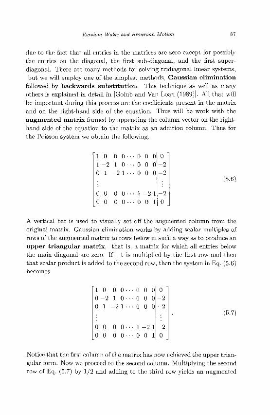
Random Walks and Brownian Motion 87
due to the fact that all entries in the matrices are zero except for possibly the entries on the diagonal, the first sub-diagonal, and the first super-diagonal. There are many methods for solving tridiagonal linear systems, but we will employ one of the simplest methods, Gaussian elimination
followed by backwards substitution. This technique as well as many others is explained in detail in [Golub and Van Loan (1989)]. All that will be important during this process are the coefficients present in the matrix and on the right-hand side of the equation. Thus will be work with the augmented matrix formed by appending the column vector on the right-hand side of the equation to the matrix as an addition column. Thus for the Poisson system we obtain the following.
1 1
0
0 0
0 - 2 1
0 0
0 0 -1 0 •
- 2 1 •
0 0 • 0 0 •
• 0 • 0 • 0
• 1 • 0
0 0 0 0 0 0
- 2 1 0 1
0 - 2 - 2
- 2 0
(5.6)
A vertical bar is used to visually set off the augmented column from the original matrix. Gaussian elimination works by adding scalar multiples of rows of the augmented matrix to rows below in such a way as to produce an upper triangular matrix, that is, a matrix for which all entries below the main diagonal are zero. If —1 is multiplied by the first row and then that scalar product is added to the second row, then the system in Eq. (5.6) becomes
1 0 0
0 0
0 - 2 1
0 0
0 0 1 0
- 2 1
0 0 0 0
0 0 0
1
0
0 0 0 0 0 0
- 2 1
0 1
0 " - 2 - 2
- 2 0
(5.7)
Notice that the first column of the matrix has now achieved the upper triangular form. Now we proceed to the second column. Multiplying the second row of Eq. (5.7) by 1/2 and adding to the third row yields an augmented
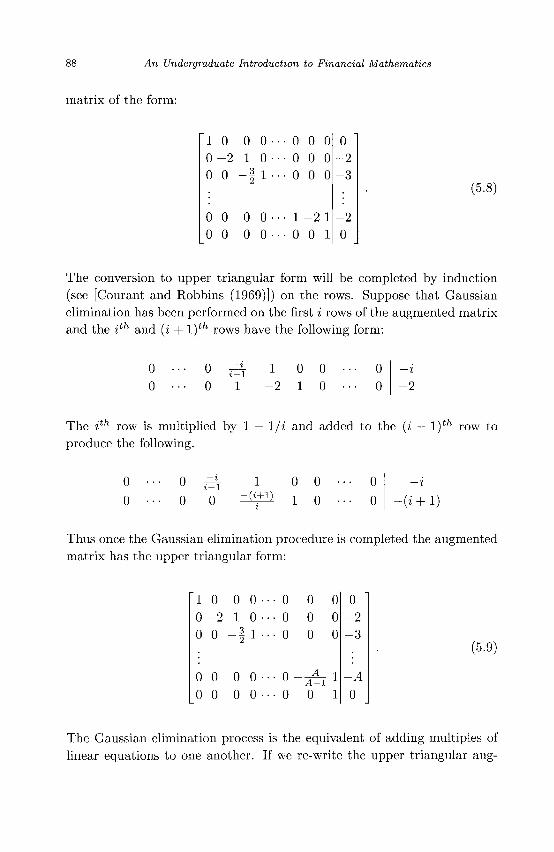
An Undergraduate Introduction to Financial Mathematics
matrix of the form:
1 0 0 - 2 0 0
0 0 0 0
0 0 1 0
- 5 1 2 x
0 0 0 0
0 0 0 0 0 0 0 0 0
1 - 2 1 0 0 1
0 " - 2 - 3
- 2
0
(5.
The conversion to upper triangular form will be completed by induction (see [Courant and Robbins (1969)]) on the rows. Suppose that Gaussian elimination has been performed on the first i rows of the augmented matrix and the ith and (i + l)th rows have the following form:
1 0 0 - 2 1 0
The i row is multiplied by 1 — 1/i and added to the (i + 1) row to produce the following.
0 -=± I — 1
0 0 -(»+!) 0 0 1 0 -(i + 1)
Thus once the Gaussian elimination procedure is completed the augmented matrix has the upper triangular form:
1 0 0 0 -
0 - 2 1 0 •
0 0 - f l -
0 0 0 0 -
0 0 0 0 -
• 0
• 0
• 0
• 0
• 0
0 0 0 0 0 0
A-l 0 1
-2 -3
-A
(5.9)
The Gaussian elimination process is the equivalent of adding multiples of linear equations to one another. If we re-write the upper triangular aug-
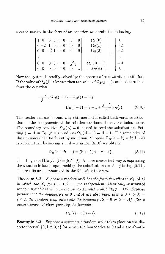
Random Walks and Brownian Motion
mented matrix in the form of an equation we obtain the following.
0 - 2 - 3
1 0 0 0 •• 0 - 2 1 0 • 0 0 - f 1 - .
0 0 0 0 •• 0 0 0 0-
• 0 • 0 • 0
• 0 -• 0
0 0 0 0 0 0
— ^ - 1 A-l i
0 1
OB(O)
fiu(l) O B ( 2 )
nB(A-VB(A)
1) 0
Now the system is readily solved by the process of backwards substitution. If the value of SIB (j) is known then the value of QB (j — 1) can be determined from the equation
J J - l
nB(j-i) + nB(j)
nB{j-i) = j - i + 3—^^B{3)- (5.10)
The reader can understand why this method if called backwards substitution — the components of the solution are found in reverse index order. The boundary condition £IB(A) = 0 is used to seed the substitution. Setting j = A in Eq. (5.10) produces QB(A — 1) = A — 1. The remainder of the unknowns can be found by induction. Suppose Q.B(A — k) = k(A — k) is known, then by setting j = A — k in Eq. (5.10) we obtain
UB{A -k-l) = {k+ I) (A - k - 1). (5.11)
Thus in general QB(A—j) = j(A—j). A more convenient way of expressing the solution is found upon making the substitution i = A — j in Eq. (5.11). The results are summarized in the following theorem.
Theorem 5.2 Suppose a random walk has the form described in Eq. (5.1) in which the Xi for i = 1,2,... are independent, identically distributed random variables taking on the values ±1 with probability p = 1/2. Suppose further that the boundaries at 0 and A are absorbing, then if 0 < 5(0) = i < A the random walk intersects the boundary (S = 0 or S = A) after a mean number of steps given by the formula
nB(i) = i(A~i). (5.12)
Example 5.2 Suppose a symmetric random walk takes place on the discrete interval {0,1, 2,3,4} for which the boundaries at 0 and 4 are absorb-
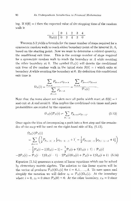
90 An Undergraduate Introduction to Financial Mathematics
ing. If 5(0) = i then the expected value of the stopping time of the random walk is
i
nB(i) 0 1 2 3 4 0 3 4 3 0
Theorem 5.2 yields a formula for the mean number of steps required for a symmetric random walk to reach either boundary point of the interval [0, A] based on the starting point. Now we want to determine a related quantity, the conditional exit time. This is the average number of steps required for a symmetric random walk to reach the boundary at A while avoiding the other boundary at 0. The symbol QA(i) will denote the conditional exit time of the random walk in the initial state 5(0) = i which exits at boundary A while avoiding the boundary at 0. By definition this conditional exit time is
/ j ^Pi — A^Pi — A / , ^Pi — A^Pi — A
,- , , . N Pi —A Pi —A
Pi—A
Note that the sums above are taken over all paths which start at 5(0) = i and exit at A and avoid 0. This implies the conditional exit times and path probabilities are related by the equation:
nA(i)VA{i) = E PP^A^Pi-A- (5.13) Pi —A
Once again the idea of decomposing a path into a first step and the remainder of the step will be used on the right-hand side of Eq. (5.13).
SlA(i)VA(i)
= /I ( 2Pp«-1^A K>(i-U-A + l\ + 2PP(i + V-A [Upii+1)-A +1]) Pi-A ^
= l-VA{i - l)nA(i - 1) + \vA(i + mA{i + 1) + VA{i)
-2PA(i) = vA{% - i)nA(i -1) - 2vA(i)nA(i) + vA{i + i)nA(i +1) (5.14)
Equation (5.14) generates a system of linear equations which can be solved by elementary matrix algebra. The solution to this linear system will be the vector of products VA{i)SlA{i) for i = 0 , 1 , . . . , A. To save space and simplify the notation we will define Zi = TA{i)QA(i)- At the boundary where i — 0, ZQ = 0 since VA(0) — 0. At the other boundary, zA = 0 since
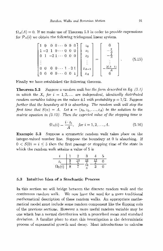
Random Walks and Brownian Motion 91
Q,A(A) = 0. If we make use of Theorem 5.1 in order to provide expressions
for VAU) we obtain the following tridiagonal linear system.
"l 0 0 0 ••• 0 0 0
1 - 2 1 0 ••• 0 0 0
0 1 - 2 1 ••• 0 0 0
0 0 0 0 ••• 1 - 2 1
0 0 0 0 ••• 0 0 1
Finally we have established the following theorem.
T h e o r e m 5.3 Suppose a random walk has the form described in Eq. (5.1)
in which the Xi for i = 1 ,2 , . . . are independent, identically distributed
random variables taking on the values ± 1 with probability p = 1/2. Suppose
further that the boundary at 0 is absorbing. The random walk will stop the
first time that S(n) = A. Let z = (zo,z\,... ,ZA) be the solution to the
matrix equation in (5.15). Then the expected value of the stopping time is
fi/iW = ^ , fori =1,2,..., A. (5.16)
E x a m p l e 5.3 Suppose a symmetric random walk takes place on the
integer-valued number line. Suppose the boundary at 0 is absorbing. If
0 < 5(0) = i < 5 then the first passage or stopping time of the s tate in
which the random walk at ta ins a value of 5 is
i Zi
n5{i)
I 8 5 8
2 14 5 7
3 16 5 16 3
4 12 5 3
5 0 0
5.3 In tu i t ive Idea of a S t o c h a s t i c P r o c e s s
In this section we will bridge between the discrete random walk and the
continuous random walk. We now have the need for a more tradit ional
mathematical description of these random walks. An appropriate mathe
matical model must include some random component like the flipping coin
of the previous sections. However a more useful random variable may be
one which has a normal distribution with a prescribed mean and s tandard
deviation. A familiar place to s tar t this investigation is the deterministic
process of exponential growth and decay. Most introductions to calculus
zo z\ z-i
ZA-\
ZA
2_ 'A
4_ A
2 ( A - 1 ) A
0
(5.15)
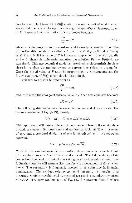
92 An Undergraduate Introduction to Financial Mathematics
(see for example [Stewart (1999)]) contain the mathematical model which states that the rate of change of a non-negative quantity P, is proportional to P. Expressed as an equation this statement becomes
dP - = ,P (5.17)
where fj, is the proportionality constant and t usually represents time. The proportionality constant is called a "growth rate" if [i > 0 and a "decay rate" if \i < 0. If the value of P is known at a specified value of t (usually at t = 0) then this differential equation has solution P{t) = P(0)eM ', see exercise 6. This mathematical model is described as deterministic since there is no place for random events to express themselves in the model. Once the initial value of P and the proportionality constant are set, the future evolution of P(t) is completely determined.
Equation (5.17) can be rewritten as
dP — =fidt, (5.18)
and if we make the change of variable X = In P then this equation becomes
dX = fidt. (5.19)
The following discussion may be easier to understand if we consider the discrete analogue of Eq. (5.19), namely
X(t + At) - X(t) = AX = fj. At. (5.20)
This equation is still deterministic but becomes stochastic if we introduce a random element. Suppose a normal random variable, dz{t) with a mean of zero and a standard deviation of one is introduced as in the following equation.
AX = nAt + <jdz(t)\TAt. (5.21)
We write the random variable as dz rather than z since we want to think of it as the change or "delta" in a random walk. The t dependency of dz comes from the need to think of z as taking on a random value at each time t. Furthermore we will assume that the dz(t) is independent of dz(s) when t T s. The constant a is frequently referred to as volatility in financial applications. The product adz{t)\/At could naturally be thought of as a normal random variable with a mean of zero and a standard deviation of a^/At. The new random part of Eq. (5.21) represents "noise" whose
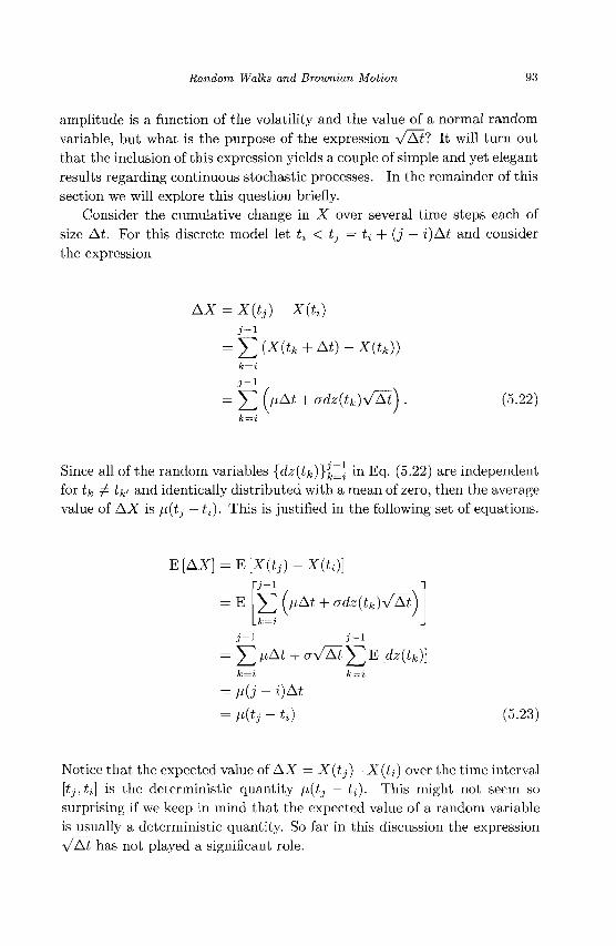
Random Walks and Brownian Motion 93
amplitude is a function of the volatility and the value of a normal random variable, but what is the purpose of the expression VAt? It will turn out that the inclusion of this expression yields a couple of simple and yet elegant results regarding continuous stochastic processes. In the remainder of this section we will explore this question briefly.
Consider the cumulative change in X over several time steps each of size At. For this discrete model let tj < tj = U + (j — i)At and consider the expression
AX = X(tj) - X(U)
= J2(X(tk + At)-X(tk)) k=i i - i ^2 (^At + crdz{tk)\f~At\ . (5.22)
Since all of the random variables {dz{tk)YkLi in Eq. (5.22) are independent for tk ^ tki and identically distributed with a mean of zero, then the average value of AX is fi(tj — U). This is justified in the following set of equations.
E[AX} = E[X(tj)-X{ti)} "i - i
^2 (fiAt + adz(tk)\/At) E
] T /iAt + ay/At ^ E [dz(tk)\ k=i k=i
fi(j - i)At
H(tj - U) (5.23)
Notice that the expected value of AX = X(tj)—X(ti) over the time interval [tj,U] is the deterministic quantity fi(tj — tj). This might not seem so surprising if we keep in mind that the expected value of a random variable is usually a deterministic quantity. So far in this discussion the expression VAt has not played a significant role.
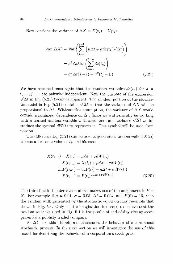
94 An Undergraduate Introduction to Financial Mathematics
Now consider the variance of AX = X(tj) — X{ti).
O'-i Var(AX) = Var I ^ (/iAt + adz(tk)V~At)
\k=i / i - i
' %)
J A . / - -\ _ Jli
cr2AtVar ^dzfa \k=i /
a2At(j -i) = a2(tj - U) (5.24)
We have assumed once again that the random variables dz(tk) for k = i,... ,j — 1 are pairwise independent. Now the purpose of the expression VAt in Eq. (5.21) becomes apparent. The random portion of the stochastic model in Eq. (5.21) contains VAi so that the variance of AX will be proportional to At. Without this assumption, the variance of AX would contain a nonlinear dependence on At. Since we will generally be working with a normal random variable with mean zero and variance %/Ai we introduce the symbol dW(t) to represent it. This symbol will be used from now on.
The difference Eq. (5.21) can be used to generate a random walk if X(ti) is known for some value of U. In this case
X{ti+1) - X{U) = fiAt + adW(U)
X{ti+l) = X{U) + fiAt + adW(U)
\nP(ti+1) =lnP(ti)+fiAt + adW(ti)
P(ti+1) = p(tl)eKAt+°dWM (5.25)
The third line in the derivation above makes use of the assignment In P = X. For example if // = 0.01, a = 0.05, At = 0.004, and P(0) = 10, then the random walk generated by the stochastic equation may resemble that shown in Fig. 5.4. Only a little imagination is needed to believe that the random walk pictured in Fig. 5.4 is the profile of end-of-day closing stock prices for a publicly traded company.
As At —> 0 this discrete model assumes the behavior of a continuous stochastic process. In the next section we will investigate the use of this model for describing the behavior of a corporation's stock price.
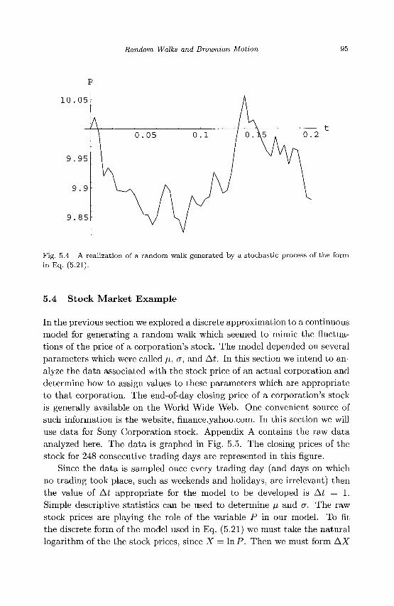
Random Walks and Brownian Motion 95
1 0 . 0 5
9 . 9 5
9 . 9
9 . 8 5
0 . 2
Fig. 5.4 A realization of a random walk generated by a stochastic process of the form in Eq. (5.21).
5.4 Stock Market Example
In the previous section we explored a discrete approximation to a continuous model for generating a random walk which seemed to mimic the fluctuations of the price of a corporation's stock. The model depended on several parameters which were called fi, a, and At. In this section we intend to analyze the data associated with the stock price of an actual corporation and determine how to assign values to these parameters which are appropriate to that corporation. The end-of-day closing price of a corporation's stock is generally available on the World Wide Web. One convenient source of such information is the website, finance.yahoo.com. In this section we will use data for Sony Corporation stock. Appendix A contains the raw data analyzed here. The data is graphed in Fig. 5.5. The closing prices of the stock for 248 consecutive trading days are represented in this figure.
Since the data is sampled once every trading day (and days on which no trading took place, such as weekends and holidays, are irrelevant) then the value of At appropriate for the model to be developed is At = 1. Simple descriptive statistics can be used to determine \x and a. The raw stock prices are playing the role of the variable P in our model. To fit the discrete form of the model used in Eq. (5.21) we must take the natural logarithm of the the stock prices, since X = In P . Then we must form AX
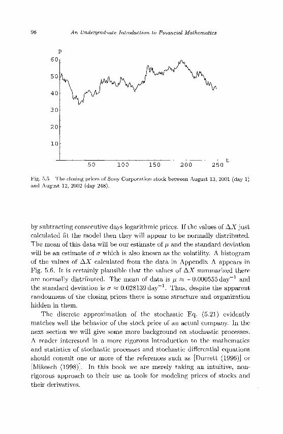
96 An Undergraduate Introduction to Financial Mathematics
P 60f A
30-
20 •
10
t 50 100 150 200 250
Fig. 5.5 The closing prices of Sony Corporation stock between August 13, 2001 (day 1) and August 12, 2002 (day 248).
by subtracting consecutive days logarithmic prices. If the values of AX just calculated fit the model then they will appear to be normally distributed. The mean of this data will be our estimate of ji and the standard deviation will be an estimate of a which is also known as the volatility. A histogram of the values of AX calculated from the data in Appendix A appears in Fig. 5.6. It is certainly plausible that the values of AX summarized there are normally distributed. The mean of data is /i « —0.000555 day - 1 and the standard deviation is a « 0.028139 day - . Thus, despite the apparent randomness of the closing prices there is some structure and organization hidden in them.
The discrete approximation of the stochastic Eq. (5.21) evidently matches well the behavior of the stock price of an actual company. In the next section we will give some more background on stochastic processes. A reader interested in a more rigorous introduction to the mathematics and statistics of stochastic processes and stochastic differential equations should consult one or more of the references such as [Durrett (1996)] or [Mikosch (1998)]. In this book we are merely taking an intuitive, nonrigorous approach to their use as tools for modeling prices of stocks and their derivatives.
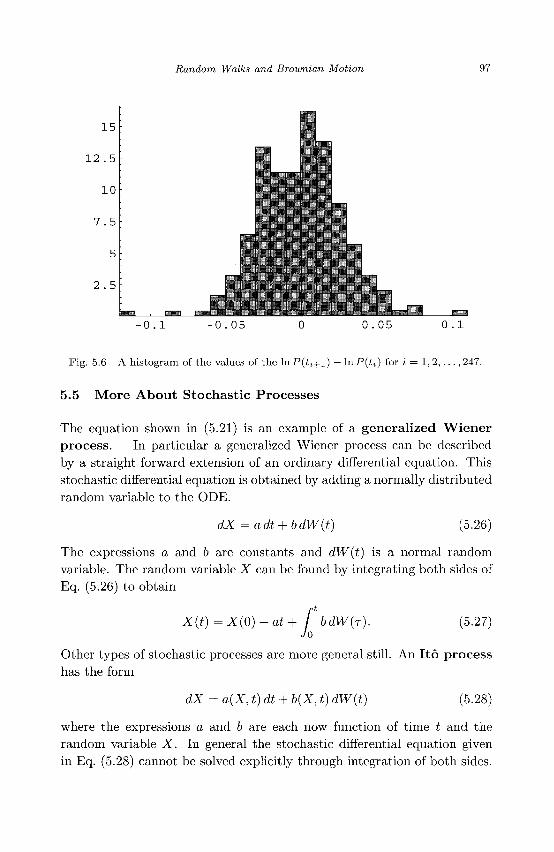
Random Walks and Brownian Motion 97
1 5
1 2 . 5
1 0
7 . 5
5
2 . 5
T J C H I
- 0 . 1 • 0 . 0 5 0 0 . 0 5 0 . 1
Fig. 5.6 A histogram of the values of the In P(ti+1) - In P(U) for i = 1, 2 , . . . , 247.
5.5 More About Stochastic Processes
The equation shown in (5.21) is an example of a generalized Wiener process. In particular a generalized Wiener process can be described by a straight forward extension of an ordinary differential equation. This stochastic differential equation is obtained by adding a normally distributed random variable to the ODE.
dX = adt + bdW(t) (5.26)
The expressions a and b are constants and dW(t) is a normal random variable. The random variable X can be found by integrating both sides of Eq. (5.26) to obtain
X(t) = X{0) + at + f bdW(r). Jo
(5.27)
Other types of stochastic processes are more general still. An Ito process has the form
dX = a(X, t) dt + b(X, t) dW{t) (5.28)
where the expressions a and b are each now function of time t and the random variable X. In general the stochastic differential equation given in Eq. (5.28) cannot be solved explicitly through integration of both sides.
98 An Undergraduate Introduction to Financial Mathematics
Nevertheless it is an important type of equation for us to use because it will enable us to work with stochastic processes of quantities which depend in turn on other random variables having their own individual stochastic process descriptions. In this way we will develop the fundamentally important Black-Scholes partial differential equation. Before we can do this we must develop an analogue of the chain rule for differentiation found in elementary calculus.
In standard differential calculus if one makes the assignment X = In P then it is well understood that dX = dP/P according to the chain rule. Using this on a generalized Wiener process may lead us to believe that the following equations are equivalent.
dX = adt + bdW(t)
dP = aPdt + bPdW(t)
First we note that while the first equation is a generalized Wiener process the second is an Ito process. Secondly, if a and b represent the mean and standard deviation respectively of random variable dX (as they did for the stock price data analyzed earlier), does the second equation imply that a and b are the mean and standard deviation of the underlying variable PI The answer is no. What is needed is a valid procedure for changing variables in a stochastic process, in other words, a stochastic calculus version of the chain rule for differentiation. This change of variable differentiation result is known as Ito's Lemma and is covered in the next section.
5.6 Ito's Lemma
The proper procedure for changing variables in a stochastic differential equation can be derived using the multivariable version of Taylor's Theorem. A standard reference containing this result is [Taylor and Mann (1983)]. Here we will give a brief overview of a two-variable version of Taylor's formula with remainder. We start with the single-variable Taylor's formula. If f(x) is an (n + l)-times differentiable function on an open interval containing XQ then the function may be written as
}(x) = /(*„) + / '(x„)(x - I„) + !-^-(x - x„f (5.29)
Random Walks and Brownian Motion 99
The last term above is usually called the Taylor remainder formula and denoted Rn+i- The quantity 9 lies between x and XQ. The other terms form a polynomial in x of degree at most n and can be used as an approximation for f(x) in a neighborhood of xo- This form of Taylor's will be used to derive the two-variable form.
Suppose the function F(y, z) has partial derivatives up to order three on an open disk containing the point with coordinates (yo,zo). Define the function f(x) = F(yo + xh, ZQ + xk) where h and k are chosen small enough that (yo + h,zo + k) lie within the disk surrounding (yo,zo). Since / is a function of a single variable then we can use the single-variable form of Taylor's formula in (5.29) with XQ = 0 and x = 1 to write
/ ( I ) = /(0) + / ' (0)x + \f'\Q)x2 + R3. (5.30)
Using the multi-variable chain rule for derivatives we have, upon differentiating f(x) and setting x = 0,
/ ' (0) = hFy(yo,z0) + kFz(y0,z0) (5.31)
/"(0) = h2Fyy(y0,zo) + 2hkFyz(y0,z0) + k2Fzz(y0,z0). (5.32)
We have made use of the fact that Fyz = Fzy for this function under the smoothness assumptions. The remainder term R3 contains only third order partial derivatives of F evaluated somewhere on the line connecting the points (yo, ZQ) and (yo + h, ZQ + k). Thus if we substitute Eqs. (5.31) and (5.32) into (5.30) we obtain
A F = / ( l ) - /(0) (5.33)
= F(y0 + h,z0 + k)- F(y0, z0)
= hFy(y0,z0) + kFz(y0, z0)
+ 5 ih2Fvy(yo,zo) + 2hkFyz(y0,z0) + k2Fzz(y0,z0)) + R3-
This last equation can be used to derive Ito's Lemma. Let X be a random variable described by an Ito process of the form
dX = a(X,t)dt + b(x,t)dW(t) (5.34)
where dW(t) is a normal random variable and a and b are functions of X and t. Let Y = F(X, t) be another random variable defined as a function of X and t. Given the Ito process which describes X we will now determine the Ito process which describes Y.
100 An Undergraduate Introduction to Financial Mathematics
Using a Taylor series expansion for Y detailed in (5.33) we find
AY = FXAX + F t At + ^FXX(AX)2 + FxtAXAt + ^Ftt{At)2 + R3
= Fx(aAt + bdW(t)) + F t At + -Fxx{aAt + bdW{t))2
+ Fxt(aAt + bdW{t))At + ^Ftt(At)2 + R3.
Upon simplifying, the expression AX has been replaced by the discrete version of the Ito process. The dependence of a and 6 on X and t has been suppressed to simplify the notation. The reader is reminded that the Taylor remainder term R3 contains terms of order (At)fc where k > 2. Thus as At becomes small
A y « Fx(aAt + bdW{t)) + Ft At + ^Fxxb2{dW(t))2.
Recall that dW{t) is a normal random variable with expected value zero and variance At. By definition
Var (dW(t)) = E [(dW(t))2] - E [dW(t)]2
which implies that E [(dW{t))2] = At which we will use as an approximation to [dW(t))2. Thus we obtain the approximation
A y « Fx{aAt + bdW(t)) + FtAt + ^Fxxb2At. (5.35)
The reader should be aware that this a merely an outline of a proof of Ito's Lemma. In particular the replacement of (dW(t))2 by At, while true, requires a more rigorous justification. The interested reader should consult [Neftci (2000), Chap. 10]. To summarize what we have done, the statement of the lemma is given below.
Lemma 5.3 (Ito's Lemma) Suppose that the random variable X is described by the ltd process
dX = a(X,t)dt + b(X,t)dW(t) (5.36)
where dW(t) is a normal random variable. Suppose the random variable Y = F(X,t). Then Y is described by the following ltd process.
dY = L(X, t)Fx + Ft + i(6(X, t))2Fxx) dt + b(X, t)FxdW{t) (5.37)
Random Walks and Brownian Motion 101
Now we can return to the question raised earlier regarding the stochastic process followed by a stock price P. If X = I nP and
dX = ndt + adW(t), (5.38)
then we can let F(X, t) = ex = P. According to Ito's Lemma then
dP = i[iex + 0 + -a2ex j dt + aex dW(t)
fi+^a2 J Pdt + aPdW{t)
Note that the coefficient of the deterministic portion of the equation contains the expression TJCT2 which would have been absent had the chain rule of deterministic calculus been used instead of Ito's Lemma. This lemma plays a role of central importance in the next chapter in which the Black-Scholes partial differential equations is derived.
5.7 Exercises
(1) Another, less formal, method for obtaining the probability that a symmetric random walk which begins in state 5(0) = i > 0 and finishes in state S = A while avoiding an absorbing boundary at 0 is to treat the Laplacian Eq. (5.4) as a continuous boundary value problem. Find all the functions f(x) which satisfy f"(x) = 0 subject to the conditions that /(0) = 0 and f(A) = 1.
(2) Another, less formal, method for obtaining the stopping time for a symmetric random walk which begins in state 0 < 5(0) = i < A and finishes in either state S = 0 or S = A is to treat the Poisson Eq. (5.5) as a continuous boundary value problem. Find all the functions g(x) which satisfy g"(x) = —2 subject to the conditions that g(0) = 0 and 9(A) = 0.
(3) If a stock price can change (up or down) by only one dollar per day and the probability of a unit increase is 1/2 what is the probability that the stock price will increase by $25 before decreasing by $50?
(4) What is the expected number of days that will elapse before the stock described in exercise 3 increases in price by $25 or decreases by $50?
(5) What is the expected number of days that will elapse before the stock described in exercise 3 increases in price by $25 while avoiding a decrease of $50?

102 An Undergraduate Introduction to Financial Mathematics
(6) Assuming that \x and -P(O) are constants, verify by differentiation and substitution that P(0)e' i t solves Eq. (5.17).
(7) Using the growth constant and volatility of the Sony Corporation stock found earlier, use Eq. (5.25) to generate a realization of the random walk of stock prices for another year's duration.
(8) Investigate the random walk of another company's stock. Collect if possible a year's worth of closing prices (P(ti) , Pfo), • • •, P(tn)) for the stock of your favorite company. Plot a histogram of AX = lnP(£j_|_i) — lnP(tj) and also calculate the mean and standard deviation of this random variable.
(9) Using the growth constant and volatility of the stock data you found in exercise 8, use Eq. (5.25) to generate a realization of the random walk of stock prices for another year's duration.
(10) Using the chain rule for derivatives from ordinary calculus (not the stochastic version governed by Ito's Lemma) verify the expressions found for / ' (0) and /"(0) in equations (5.31) and (5.32). Find an expression for the Taylor remainder P3.
(11) Suppose that P is governed by the stochastic process
dP = nPdt + oPdW{t)
and that Y = Pn. Find the process which governs Y.
(12) Suppose that P is governed by the stochastic process
dP = fiPdt + aP dW(t)
and that Y = In P . Find the process which governs Y.

Chapter 6
Options
In the present world of finance there are many types of financial instruments which go by the name of options. At its simplest, an option is the right, but not the obligation, to buy or sell a security such as a stock for an agreed upon price at some time in the future. The agreed upon price for buying or selling the security is known as the strike price. Options come with a time limit at which (or prior to) they must be exercised or else they expire and become worthless. The deadline by which they must be exercised is known as the exercise time, strike time, or expiry date. In the remainder of the text the three terms will be used interchangeably. An option to buy a security in the future is called a call option. An option to sell is known as a put option. Types of options can also be distinguished by their handling of the expiry date. The European option can only be exercised at maturity, while an American option can be exercised at or before the strike time. Of the two types, the European option is simpler to treat mathematically, and will be the focus of much of the rest of this book. However, in practice, American options are more commonly traded. There is a mathematical price to be paid in terms of complexity for the added flexibility of the American-style option.
Suppose stock in a certain company is selling today for $100 per share. An investor may not want to buy this stock today, but may want to own it in the future. To reduce the risk of financial loss due to a potential large increase in the price of the stock during the next three-month period, they buy a European call option on the stock with a three-month strike time and a strike price of $110. At the expiry date, if the price of the stock is above $110 and the investor now wishes to buy the stock, they have the right as holder of the call option to purchase it for $110, even if the market value of the stock is higher. Otherwise if the value of the stock is below
103
104 An Undergraduate Introduction to Financial Mathematics
$110 and the investor still wishes to buy the stock, they will let the call option expire without exercising it, and purchase the stock at its market price. Call options allow investors to protect themselves against paying an unexpectedly high price in the future for a stock which they are considering purchasing.
We have used the language of "buying" an option. Thus options themselves have some value, just as the securities which underlie the options have a value. An important issue to consider is how are values assigned to options? In light of the Arbitrage Theorem of Chapter 4, if the option is mis-priced relative to the security, arbitrage opportunities may be created. In this chapter we will explore some of the relationships between option and security prices. We will derive the Black-Scholes partial differential equation, together with boundary and final conditions which govern the prices of European call options.
During the explanations of many of the concepts in this chapter, we will refer to buying or selling a financial instrument. In the financial markets it is often possible to sell something which we do not yet own by borrowing the object from a true owner. For example investor A may borrow 100 shares of stock from investor B and sell them with the understanding that by some time in the future investor A will purchase 100 shares of the same stock and return them to investor B. Normally one buys an object first and sells it later, but in the financial arena one can often sell first and then buy later. Borrowing and selling an object with the agreement to purchase it later is called adopting a short position in the object, or sometimes shorting the object. Adopting a short position can be a profitable transaction if the investor believes the price of the object is going to decrease. Purchasing an object first and then selling it in the future is called adopting a long position.
6.1 Properties of Options
There are many relationships between the values of options and their underlying securities. The maintenance of most of these relationships is necessary to eliminate the possibility of arbitrage. We will cover some these relationships here and give the reader a taste of the way that one can prove these properties. Throughout this section we will use the following definitions.
Ca: value of an American-style call option Ce: value of a European-style call option
Options 105
K: strike price of an option Pa: value of an American-style put option Pe: value of a European-style put option r: continuously compounded, risk-free interest rate S: price of a share of a security T: exercise time of an option
We have used the term "risk-free" to describe the interest rate r. It is assumed that this is the rate of return of an investment which carries no risk. While the reader may wish to debate whether a complete absence of risk can ever be achieved, there are some investments which carry very little risk, for example, U.S. Treasury Bonds.
Consider the cost of an American option compared with a European option. In the absence of arbitrage an American-style option must be worth at least as much as its European counterpart, i.e. Ca > Ce and Pa > Pe. Naturally we are assuming that the strike prices, strike times, and underlying securities are the same. To the contrary, suppose that Ca < Ce. Taking the position of an informed consumer, knowing that the American-style option has all the characteristics of the European option and in addition has the increased flexibility that it may be exercised early, no investor would purchase a European-style call option if it cost more than the American-style option. To formulate a more mathematical proof, suppose an investor sells the European-style call option and purchases the American-style option. Since Ce — Ca > 0, the investor may purchase a risk-free bond paying interest at rate r compounded continuously. At the expiry date the bond will have value (Ce — Ca)e
rT. If the owner of the European option wishes to exercise the option, the investor insures this is possible by exercising their own American option. If the owner of the European option lets it expire unused, then the investor can do the same with the American option. Thus in both cases the investor makes a risk-free profit of (Ce — Ca)e
rT which is an example of arbitrage.
It is also the case that Ce > S—Ke~rT or arbitrage is present. Assuming an absence of arbitrage and that Ce < S — Ke~rT, an investor can purchase the call option and sell the security at time t = 0. Since 0 < Ke~rT < S — Ce, the investor can invest S — Ce in a risk-free bond paying interest rate r. At the strike time the bond is worth (S — Ce)e
rT which is greater than K. Thus if the investor chooses to exercise the option (because S at time T is greater than K), the bond can be cashed out, the security purchased for K, and there is still capital left over. In other words there is risk-free
106 An Undergraduate Introduction to Financial Mathematics
profit. On the other hand if S at time T is less than K, the short position on the security is eliminated using the bond and purchasing the stock for S (which is less than K). Again there will still be capital left over. Once again there is a risk-free profit.
There is strict arbitrage-free relationship between the value of a European call and put with the same strike price and expiry date on the same underlying security. This is the important Put-Call Parity Formula of Eq. (6.1).
Pe + S = Ce + Ke'rT (6.1)
To see why this relationship must be true, imagine portfolio A represents the left-hand side of (6.1) while the right-hand side is represented by portfolio B. The Put-Call Parity Formula implies that in an arbitrage-free setting these portfolios must have the same value.
Suppose portfolio A is worth less than portfolio B, i.e.
Pe + S <Ce + Ke~rT. (6.2)
An investor can borrow at interest rate r an amount equal to Pe + S — Ce. This would allow the investor to purchase the security, the European put option, and to sell the European call option. At the strike time of the two options, the investor must repay principal and interest in the amount of (Pe + S — Ce)e
rT. If the security is worth more than K at time T, the put expires worthless and the call will be exercised by its owner. The investor must sell the security for K. Thus the net proceeds of this transaction are
K~{Pe + S- Ce)erT > 0 (6.3)
since inequality (6.3) is equivalent to the one in (6.2). If the security is worth less than K at time T, the call expires worthless and the put will be exercised by the investor. Again the investor will sell the security for K. The net proceeds of this transaction are the same as in the previous case. Thus there is a risk-free profit to be realized if portfolio A is worth less than portfolio B.
Now suppose portfolio A is worth more than portfolio B, i.e.
Pe + S>Ce + Ke~rT. (6.4)
An investor can sell the security and the European put option and buy the call option. This generates an initial positive flow of capital in the amount of S + Pe — Ce. This amount will be invested in a risk-free bond earning
Options 107
interest at rate r until the expiry date arrives. At that time the investor will have (S + Pe — Ce)e
rT. If the security is worth more than K at time T, then the put option is worthless and investor will exercise the call option. The investor purchases the security for K (thus canceling their short position). This leaves the investor with a net gain of
(Pe + S - Ce)erT -K>0 (6.5)
since inequality (6.5) is equivalent to the one in (6.4). If the security is worth less than K at time T, the call option expires unused and the owner of the put option will exercise it. Thus the investor will clear their short position by buying the security for K and their net gain is as before. Consequently there exists an arbitrage opportunity if portfolio B is worth less than portfolio A. Therefore the two portfolios must have the same value, i.e. the Put-Call Parity Formula is true.
Assuming that the prices of European call and put options are non-negative (a mild assumption), we can derive two corollary inequalities to the Put-Call Parity Formula.
Ce > S - Ke~rT (6.6)
Pe > S + Ke~rT (6.7)
While none of the formulas or inequalities developed so far enable us to price options directly, they are useful checks for arbitrage opportunities.
6.2 Pricing an Option Using a Binary Model
In this section we will examine a very simple option/security situation and determine the arbitrage-free price for the security. The analysis done here is too simple to be applied directly to any real-world example of a security; however, it provides an example application of the Arbitrage Theorem (Theorem 4.4). This type of analysis can be generalized and extended to more relevant real-world examples and thus provides a good starting point for the goal of developing option pricing formulae. The analysis performed here is based on a binary model, so named since the security is assumed to take on one of two values in the future.
Suppose the price of a share of stock is $100 currently. After a single, indivisible unit of time T, the price of the share will either be $50 or $200. The stock will be worth $50 after time T with probability p or will be worth $200 with probability 1 — p. Currently an investor can purchase a
108 An Undergraduate Introduction to Financial Mathematics
European call option whose value is C. The exercise time and strike price of the option are respectively T and $150. In the absence of arbitrage what is the value of CI
The investor could buy either the option or the stock at the beginning of the time interval. In the absence of arbitrage, the expected value of the investor's profit from either course of action should be zero regardless of which direction the price of the stock moves. Since the option or stock may be purchased at the beginning of the time interval but the profit (if any) arrives after time T has elapsed, we must calculate the present value of any potential profit. We will assume the interest rate per T unit of time is r. Suppose the investor purchases the stock initially. At time T their net gain is -100 + 200(1 + r ) _ 1 with probability p or -100 + 50(1 + r ) _ 1 with probability 1 — p. In an arbitrage-free setting the expected value of this gain is zero.
-100 + 50(1 +r)-1)(l-p) 0 =
0 =
p =
-- (-100 + 200(1 + r)'1)p+ (
= -100(1+ r) + 150p +50 l + 2r
On the other hand, if the investor purchases the option initially, at time T their net gain is -C + (200 - 150)(1 + r ) " 1 with probability p or — C with probability 1 — p. Again the expected value of this gain will be zero in the absence of arbitrage.
0 = ( - C + 5 0 ( l + r ) " 1 ) p + ( - C ) ( l - p )
0 = SO^l + r ) " 1 -C
C = 5° + 1 0 0 ; (6.9) 3(l + r) V ;
Equation (6.9) was found using Eq. (6.8). The arbitrage-free probability vector and the option cost both depend on the interest rate. Figure 6.1 contains a parametric plot of the points (p(r),C(r)). If the probability p and the call option price deviate from the curve shown, then a risk-free profit can be made.
Example 6.1 Suppose the current value of the stock is 5(0) = $100 and a time T = 1
_ J $ 2 0 0 w i t h Probability p = 11/30, ^ ' ~ \ $50 with probability l-p= 19/30.
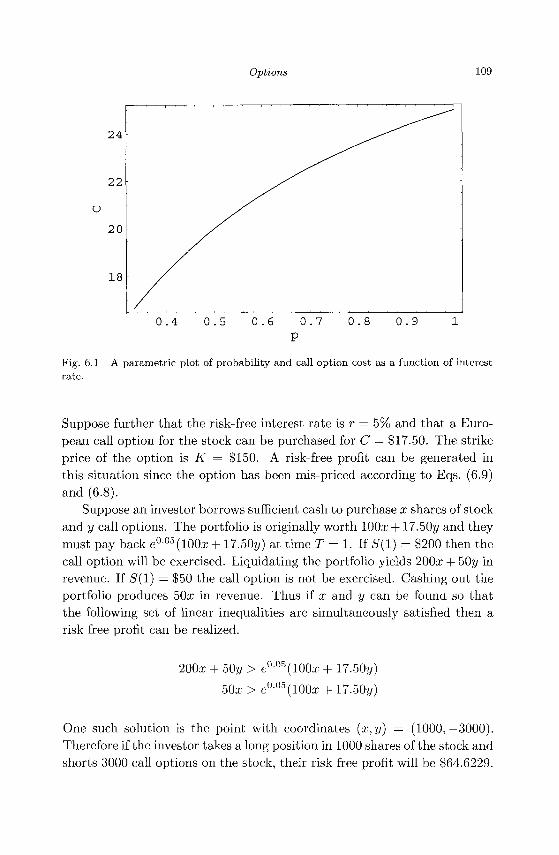
Options 109
0 . 4 0 . 5 0 . 6 0 . 7 0 . 8 0 . 9 1
P
Fig. 6.1 A parametric plot of probability and call option cost as a function of interest rate.
Suppose further that the risk-free interest rate is r = 5% and that a European call option for the stock can be purchased for C = $17.50. The strike price of the option is K = $150. A risk-free profit can be generated in this situation since the option has been mis-priced according to Eqs. (6.9) and (6.8).
Suppose an investor borrows sufficient cash to purchase x shares of stock and y call options. The portfolio is originally worth 100a; + 17.50y and they must pay back e005(100a; + 17.50y) at time T = 1. If 5(1) = $200 then the call option will be exercised. Liquidating the portfolio yields 200a; + 50y in revenue. If 5(1) = $50 the call option is not be exercised. Cashing out the portfolio produces 50a; in revenue. Thus if x and y can be found so that the following set of linear inequalities are simultaneously satisfied then a risk free profit can be realized.
200a; + 50y > e005(100a: + 17.50y)
50a; > e°-05(100a;+17.50y)
One such solution is the point with coordinates (x,y) = (1000,-3000). Therefore if the investor takes a long position in 1000 shares of the stock and shorts 3000 call options on the stock, their risk-free profit will be $64.6229.
22
U
20
110 An Undergraduate Introduction to Financial Mathematics
6.3 Black-Scholes Partial Differential Equation
In this section we will derive the fundamental equation governing the pricing of options, the famous Black-Scholes partial differential equation. The ideas of arbitrage, stochastic processes, and present value converge at this point in the study of financial mathematics.
We begin by supposing that S is the current value of a security and that it obeys a stochastic process of the form
dS Sdt + aSdW(t) (6.10)
If F(S, t) is the value of any type of option (more generally called a financial derivative), then according to Ito's Lemma (Lemma 5.3), F obeys the following stochastic process.
dF = H + SFS + \a2S2Fss + F^\ dt + aSFs,dW(t) (6.11)
Suppose a portfolio of value P is created by selling the option and buying A units of the security. Thus the value of the portfolio is P = F — AS. Since the portfolio is a linear combination of the the option and the security then the stochastic process governing the portfolio is
dP = d(F - AS)
dF - AdS
( \ ^1 SFS + \a2S2Fss + Ft\
+ A [ [ f i + y j S ( f t + (7S(iW(t))
(
r a2" S[Fs-A} + ^a2S2Fss
+ aS (Fs - A) dW(t)
Ft\dt
(6.12)
Notice the coefficient of the normal random variable, dW(t), contains the factor Fs — A. Equation (6.12) can be simplified if we assume A = Fs-This has the beneficial effect of reducing the number of stochastic terms in Eq. (6.12). Randomness is not completely eliminated since the value of the security S remains and is stochastic. Under the assumption that A = -Fs,
Options 111
Eq. (6.12) becomes
dP=(^a2S2Fss + F?jdt. (6.13)
In an arbitrage-free setting the difference in the returns from investing in the portfolio described above or investing an equal amount of capital in a risk-free bond paying interest at rate r should be zero. Thus the following equations are true.
0 = rPdt-dP
0 = rPdt- (^a2S2Fss + Ft} dt
rP = l-a2S2FSS + Ft
r(F - AS) = l-a2S2Fss + Ft
rF = ^a2S2Fss + Ft + rAS
rF = Ft+ rSFs + ^<x2S2Fss (6.14)
Equation (6.14) is an example of a partial differential equation or PDE, for short. While the general theory of solving PDEs is beyond the scope of this book, we will briefly mention a few concepts related to the Black-Scholes PDE. PDEs are often described by their order, type, and linearity properties. The Black-Scholes PDE is a second order equation since the highest order derivative of the unknown function F present in the the equation is the second derivative. This PDE is of parabolic type. The best known example of the parabolic PDE is the heat equation which is used to describe the distribution of temperature along an object, for example a metal rod. For an introductory treatment of the heat equation see [Boyce and DiPrima (2001)]. In [Wilmott et al. (1995)] the Black-Scholes PDE is solved by appropriate changes of variables until it becomes the heat equation, which is easily solved via a technique known as separation of variables. Lastly, the Black-Scholes PDE is an example of a linear partial differential equation since if F\ and F^ are two solutions to the equation then c\F\ + C2-F2 is also a solution where c\ and c^ are any constants (see exercise 9).
Financial derivative products of many types obey the Black-Scholes equation. Different solutions correspond to different initial/final and
112 An Undergraduate Introduction to Financial Mathematics
boundary side conditions imposed while solving the equation. In the next section we will describe in more detail the initial and boundary conditions relevant to the Black-Scholes PDE. In Sec. 7.4 we will derive a solution to the Black-Scholes equation for the price of a European style call option.
6.4 Boundary and Initial Conditions
Without the imposition of side conditions in the form of initial or final conditions and boundary conditions, a partial differential equation can have many different solutions. Mathematicians refer to a differential equation with many possible solutions as "ill-posed." In this section we will discuss the appropriate conditions to impose in order to obtain a solution to Eq. (6.14) which describes the value of a European call option.
The domain of the unknown function F of Eq. (6.14) is a region in (S, t)-space. We will refer to this region as f2 C (5, £)-space. For a European call option we are only interested in the value of the option during the time interval [0,T], where T is the exercise time of the option. During this time interval the price of the security underlying the option may be any non-negative value. Thus the domain of the solution to Eq. (6.14) is
Q = { ( S , i ) | 0 < S < ooandO < t < T}.
At time t = T the value of the security will either exceed the strike price (in which case the call option will be exercised generating an income flow of S(T) — K > 0) or the security will have a value less than or equal to the strike price (in which case the call option expires unused and has value 0). When S(T) > K the call option is said to be in the money. When S(T) < K the call option is said to be out of the money. Thus the terminal value of a European call option is
(S(T) - K)+ = max{5(T) - K, 0},
where S(T) is the value of the underlying security at the exercise time and K is the strike price of the option. Graphically the payoff of the portfolio is said to resemble a "hockey stick". See Fig. 6.2. Hence we can use the following equation as the final condition of the Black-Scholes PDE.
F(S,T)=m&x{S{T)-K,0} (6.15)
Since there is a final condition and no initial condition, the Black-Scholes PDE is sometimes referred to as a backwards parabolic equation.

Options 113
( S ( T ) - K ) +
S ( T )
Fig. 6.2 The piecewise linear curve representing the payoff of a European call option.
We see from Eq. (6.10) that if S = 0, then dS = 0, i.e. S never changes and hence remains zero. The state S — 0 is an absorbing boundary condition for the random walk of S. Thus on the portion of the boundary of ft where 5 = 0, the call option would never be exercised and hence must have zero value. Thus we have derived one boundary condition, namely
F(0,i) = 0. (6.16)
Now if we suppose that S is approaching infinity, it becomes increasingly likely that the call option will be exercised, since as S —> oo, S will exceed any finite value of K. Also as S —> oo, the difference S — K fa S and hence we have the remaining boundary condition
F(S, t) = S, as S -> oo. (6.17)
Thus to summarize the Black-Scholes equation and its final and boundary conditions for a European call option we have the following set of equations.
rF = Ft + rSFs + ^a2S2Fss for (S, t) in ft,
F(S, T) = (S(T) - K)+ for 5* > 0,
F(0,t) = 0 for0<i<T,
F{S,t) = S asS-^oo.
114 An Undergraduate Introduction to Financial Mathematics
6.5 Exercises
(1) Show that in the absence of arbitrage Pa > Pe where the underlying security, exercise time, and strike price for both options are the same.
(2) Consider a European call option with a strike price of $60 which costs $10. Draw a graph illustrating the net payoff of the option for stock prices in the interval [0,100].
(3) Show that in the absence of arbitrage the value of a call option never exceeds the value of the underlying security.
(4) What is the minimum price of a European style call option with an exercise time of three months and a strike price of $26 for a security whose current value is $29 while the continuously compounded interest rate is 6%?
(5) If a share of a security is currently selling for $31, a three-month European call option is $3 with a strike price of $31, and the risk-free interest rate is 10%, what is the arbitrage-free European put option price for the security?
(6) If a share of a security is currently selling for $31, a three-month European call option is $3, a three-month European put option is $2.25, and the risk-free interest rate is 10%, what is the arbitrage-free strike price for the security?
(7) What is the minimum price of a European put option with an exercise time of two months and a strike price of $14 for a stock whose value is $11 while the continuously compounded interest rate is 7%?
(8) If a share of a security is currently selling for $31, a three-month European call option is $3, a three-month European put option is $1, the strike price for both options is $30, and the risk-free interest rate is 10%, what arbitrage opportunities are open to investors?
(9) Suppose the functions fi(S, t) and /2(5, t) each solve the Black-Scholes Eq. (7.5). Show that if c\ and ci are constants then the function f(S,t) = c\fi(S,t) + C2f2(S,t) also solves the Black-Scholes equation.
(10) What final and boundary conditions are appropriate for the Black-Scholes PDE (6.14) when F represents a European-style put option?
Chapter 7
Solution of the Black-Scholes Equation
In Chapter 6 the Black-Scholes partial differential equation was derived and summarized in Eq. (6.14). Every European style option satisfies this PDE. The differences in the options are due to different boundary and final conditions. In the present chapter we will solve the Black-Scholes equation with boundary and final conditions appropriate for a European style call option. Several methods are available to solve this equation. Some take the limit of a discrete time binomial model of security prices (see [Ross (1999)]). In [Wilmott et al. (1995)] the Black-Scholes PDE is transformed through a sequence of changes of variable to an ordinary differential equation which is solved by elementary means. Their change of variable approach will be mimicked here, but the Fourier Transform will be used to solve the equation. For readers unfamiliar with the Fourier Transform, a brief introduction to the relevant operations are included in this chapter. The Fourier Transform is a standard mathematical device used to convert certain types of partial differential equations into ordinary differential equations. A more complete introduction to the Fourier Transform can be found in either [Greenberg (1998)] or [Jeffrey (2002)].
7.1 Fourier Transforms
Suppose the function f(x) is defined for all real numbers, and that The Fourier Transform of / is denoted T{f{x)} or often as f(w). By definition the Fourier Transform of / is
/
oo
f(x)e-*wxdx, (7.1) -OO
115
116 An Undergraduate Introduction to Financial Mathematics
provided the improper integral converges. There are many theorems in the literature on the Fourier Transform which list conditions under which the Fourier Transform will exist. It is possible to state very general but technical conditions in such an existence theorem. For our purposes we will adopt a less technical theorem which states that if the domain of / is all real numbers and if
• / and / ' are piecewise continuous on every interval of the form [-M, M) for arbitrary M > 0, and
/
oo \f(x)\dx converges,
-oo
then the Fourier Transform of / exists according to Theorem 17.9.1 of [Greenberg (1998)]. The symbol i = \/—T. The Fourier Transform maps the original function / which is a function of a; to a new function / which depends on w which is often thought of as a frequency.
Example 7.1 Consider the piecewise-defined function
/ ( s ) = / l i f M < l [ 0 otherwise.
Its Fourier Transform is readily found through the following calculation.
POO
/ H = / f(x)e-iwxdx
/ ;
= — - (e-iw -eiw)
iw 2
= — sin w w
In the previous example we carried out integration of a complex exponential as if it followed the same rules of integration as real-values functions. This is in fact true. The Euler Identity, e10 = cos 8 + i sin 9 was also used to simplify the result [Churchill et. al. (1976)].
The Fourier Transform also has an interesting effect on derivatives of functions. Suppose the Fourier Transform of / exists and that / is differ-
Solution of the Black-Scholes Equation 117
entiable for all real numbers.
/oo
-OO
/OO
f(x)(-iw)e -oo
/
OO
f(x)e~iwx dx -OO
= iwf(w) (7.2) The technique of integration by parts was used to shift the derivative off of / and onto the exponential function. Since / vanishes as \x\ —> oo the leading integral is zero. This property of the Fourier Transform can be extended to higher order derivatives.
Theorem 7.1 If f(x), f'(x), . . . , f^n~1\x) are all Fourier transformable and if f{n){x) exists (where neN) then F{f(n)(x)} = {iw)nf{w).
Proof. The result has already been shown in Eq. (7.2) for the case where n = 1. The technique of proof by induction is used to establish this result for all higher order derivatives. Suppose the result has been proved for n = k.
F{f(k+l\x)}= f{k+1) (x)e~iwx dx J —OO
oo r°° = f(k\x)e-iwx - f(k\x)(-iw)e-iwxdx
- O O
/
OO
f(k){x)e -OO
iw / f^(x)e-lwxdx
= iw(iw)kf{w) = (iw)k+1f(w)
The induction assumption was used in the second to the last line of this equation. •
Another Fourier Transform result which we will have need for later concerns the transform of the convolution of two functions. By definition the Fourier Convolution of two functions / and g is
/
OO
f(x-z)g(z)dz. (7.3)
-oo
The Fourier Convolution is not the same as the Fourier Transform. The convolution involves no complex integration, merely the integration of the
118 An Undergraduate Introduction to Financial Mathematics
product of two real-valued functions. It is possible to calculate the Fourier Transform of this convolution.
Theorem 7.2 F{(f * g)(x)} = f{w)g(w), in other words the Fourier Transform of the Fourier Convolution of f and g is the product of the Fourier Transforms of f and g.
Proof. We begin by applying the definitions of Fourier Transform and Convolution.
/
oo r />oo
/ f{x-z)g{z)dz
" /»O0
/ f(x-z)g(z)e-iwxdz .J —oo J.
oo oo
oo !_•/ — oo oo
f(x - z)g(z)e~
/
oo r /»oo
g{z) / f(x - z)e -oo J— oo
lwxdx
~iwx dx
' dx
dx
dz
dz
Since the order of integration in a multiple integral is irrelevant (only the region over which the integration takes place is meaningful), equality is preserved above. Now the change of variable x = u + z is used to rewrite the interior integral above.
/
oo r />oo
g(z) / /(«)e-™<»+ '>dU -oo l_« — oo
g(z)e )
/
oo
g(z)e -oo
= f{w)g{w)
dz
J00 g{z)e-™Af J—oo \_J —
f(u)e~
•IWZ dz
du dz
U
7.2 Inverse Fourier Transforms
So far we have seen that the Fourier Transform can be used to map functions of x, their derivatives, and their convolutions to other functions which depend on a frequency-like variable w. We intend to apply this transformation to the Black-Scholes partial differential equation and its associated side conditions. However, any useful solution to the Black-Scholes equation
Solution of the Black-Scholes Equation 119
should depend on the variables and constants in the original equation and not on the frequency variable w. It is necessary to have a method for transforming a function of w back into a function of x. This is the purpose of the Inverse Fourier Transform. By definition the inverse Fourier Transform of f(w) given by
^HfM} = ^J fMelwx dw. (7.4)
Example 7.2 Suppose a is a positive constant, then the inverse Fourier Transform of e_a''!"' is
1 f°° T-lre-a\wh = _ / -a\w\ iwxd
oo
0 -i /•oo 1 /" 1 /* _ / e(a+ix)wdw+_ / (-a+ix)«,d
2?r J^ 2TT J0 -oo ^ " JO
1 1 27r(a + ix) 2ix{a — ix)
a
7r(a2 + a;2)
Readers with some prior exposure to the Fourier Transform may prefer more symmetric definitions of the transform and the inverse transform. An infinite number of variations on the formulas can be stated, though they are all equivalent and compatible with the versions given above in Eqs. (7.1) and (7.4). Some people prefer each of the forward and inverse transforms to be scaled by a factor involving ^/2TT as in the following.
7.3 Changing Variables in the Black-Scholes P D E
To recap the partial differential equation and its side conditions for a European style call option, we have the following three equations
rF = Ft + -a2S2Fss + rSFs for t € [0, T), S G (0, oo) (7.5)
F(S, T) = (K- S)+ for S € (0, oo) (7.6)
F(0, t) = 0, F{S, t)->S as S -+ oo for t G [0, T). (7.7)
120 An Undergraduate Introduction to Financial Mathematics
The final condition given in (7.6) states tha t when the expiry date for
the option arrives, the call option will be worth nothing if the value of the
stock is less than the strike price. Otherwise the call option is worth the
excess of the stock's value over the strike price. The boundary conditions
are specified in Eq. (7.7). The first condition implies tha t if the stock itself
becomes worthless before maturity, the call option is also worthless. An
investor could buy the stock for nothing and then let the call option expire
unused. The second part of this condition follows from the European call
option property discussed in Chapter 6, namely Ce > S — Ke~rT. Thus as
S —> oo the value of the call option becomes S asymptotically.
A judicious change of variables for the Black-Scholes equation can sim
plify it. In fact, in only a few steps we can convert Eq. (7.5) into a more well
known partial differential equation, namely the H e a t Equat ion . Suppose
F, S, and t are defined in terms of the new variables v, x, and r as in the
following equations.
S = Kex «• x = In (7.8)
t = T-^^r=^-(T-t) (7.9)
F(S,t) = KV{X,T) (7.10)
How are the Black-Scholes equation and its side conditions altered by this
change of variables? The multivariable form of the chain rule can be used
to determine new expressions for the derivatives present in Eq. (7.5).
Fs = (Kv(x,T))S = K (VXXS + vtts) = K (vx^ + o\ = e~xvx (7.11)
The reader will be asked to verify tha t
and (7.12)
'*) (7-13)
in exercises 4 and 5. Substi tuting the results in Eqs. (7.10)-(7.13) in the
Black-Scholes Eq. (7.5) and simplifying produces the equation
vT = vxx + (k- l)vx - kv (7.14)
where k = 2r/a2 (see exercise 6).
Ft
Fss
Ka2
„-2z
K \Vxx
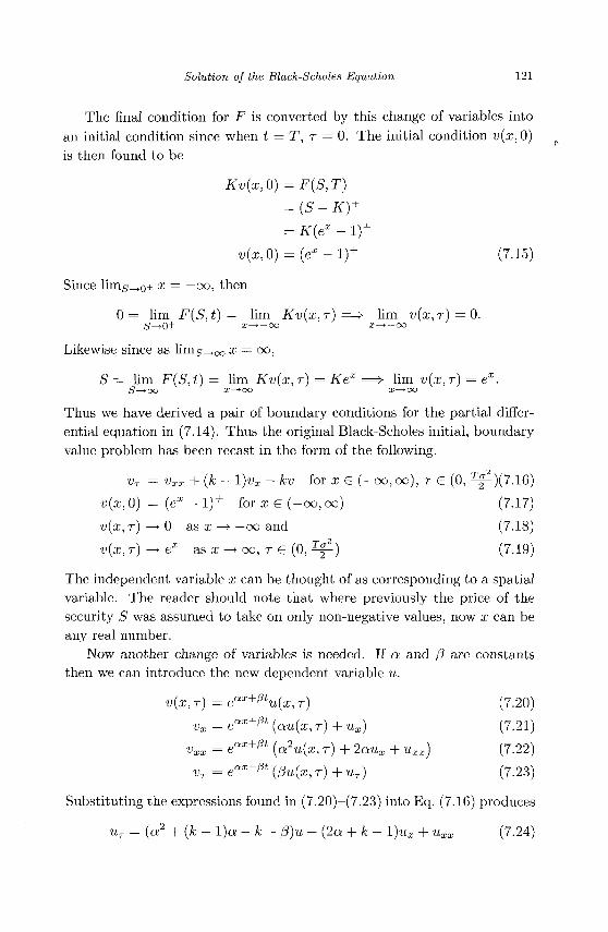
Solution of the Black-Scholes Equation 121
The final condition for F is converted by this change of variables into an initial condition since when t = T, r = 0. The initial condition v(x,0) is then found to be
Kv(x,0) =F(S,T)
= (S-K)+
= K(ex - 1)+
v(x, 0) = (ex - 1)+ (7.15)
Since lims^0+ x = —°°: then
0 = lim F(S,t) = lim KV(X,T) =$• lim V(X,T)=0. g_>0+ x—> — oo x—> — oo
Likewise since as linig^oo x — oo,
S = lim F(S,t) = lim KV(X,T) = Kex =^ lim v{x,r) = ex. S—^oo x—^oo x—>oo
Thus we have derived a pair of boundary conditions for the partial differential equation in (7.14). Thus the original Black-Scholes initial, boundary value problem has been recast in the form of the following.
vT = vxx + (k — l)vx — kv for x G (—oo, oo), r 6 (0, ^|-)(7.16)
v{x, 0) = (ex - 1)+ for x G (-oo, oo) (7.17)
V(X,T) —> 0 as x —> —oo and (7-18)
v(x,r)^ex as x ^ o o , r G (0, ^ ) (7.19)
The independent variable x can be thought of as corresponding to a spatial variable. The reader should note that where previously the price of the security S was assumed to take on only non-negative values, now x can be any real number.
Now another change of variables is needed. If a and (3 are constants then we can introduce the new dependent variable u.
V{X,T) = eax+l3tu(x,T) (7.20)
vx=eax+l3t(au(x,T)+ux) (7.21)
Vxx & ax+pt (a2u{x,T)+2aux+uxx) (7.22)
vT = eax+f3t ([3u(x, T) + uT) (7.23)
Substituting the expressions found in (7.20)-(7.23) into Eq. (7.16) produces
uT = (a2 + (k - l)a - k - j3)u + (2a + k - l)ux + uxx (7.24)
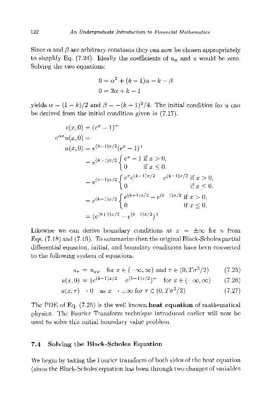
122 An Undergraduate Introduction to Financial Mathematics
Since a and /3 are arbitrary constants they can now be chosen appropriately to simplify Eq. (7.24). Ideally the coefficients of ux and u would be zero. Solving the two equations:
0 = a2 + (k - l ) a - k - /3
0 = 2a + k-l
yields a = (1 — k)/2 and (3 = —{k + l ) 2 /4 . The initial condition for u can be derived from the initial condition given in (7.17).
v(x,0) = ( e x - l ) +
eaxu(x,0) =
u{x,0) = eC=-iW2(e* _ i)+
=(fc-i)z/2 / ex - 1 if x > 0, 0 i f x < 0 .
(fc-i)x/2 f exe^k'^xl2 - e^ - 1 ) - / 2 if x > 0, 6 | 0 if x < 0.
= p ( f e - i W 2 f e ( f c + 1 W 2 - e ( f c - 1 W 2 i f a ; > 0 , \ 0 if x < 0.
= (e(fc+l)x/2 _ e(k-\)x/2-s +
Likewise we can derive boundary conditions at x = ±oo for u from Eqs. (7.18) and (7.19). To summarize then the original Black-Scholes partial differential equation, initial, and boundary conditions have been converted to the following system of equations.
uT = uxx for x G (—00,00) and r S (0,T<r2/2) (7.25)
u(x, 0) = (e{k+l>'2 - e(fc-iW2)+ for x G (-oo, 00) (7.26)
u(x, r) -^ 0 as x -> ±00 for r G (0, T<r2/2) (7.27)
The PDE of Eq. (7.25) is the well-known heat equation of mathematical physics. The Fourier Transform technique introduced earlier will now be used to solve this initial boundary value problem.
7.4 Solving the Black-Scholes Equation
We begin by taking the Fourier transform of both sides of the heat equation (since the Black-Scholes equation has been through two changes of variables
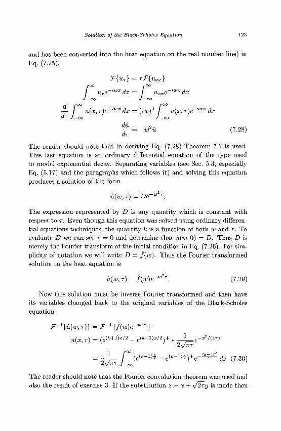
Solution of the Black-Scholes Equation 123
and has been converted into the heat equation on the real number line) in Eq. (7.25).
T{ur) = TT{UXX\
/
OO rOO
uTe~iwxdx = \ uxxe~iwxdx -oo J — oo
— u{x,r)e~lwx dx = (iw)2 u{x,r)e ®^ J — oo J ~ oo
— = -w2u (7.28) dr
The reader should note that in deriving Eq. (7.28) Theorem 7.1 is used. This last equation is an ordinary differential equation of the type used to model exponential decay. Separating variables (see Sec. 5.3, especially Eq. (5.17) and the paragraphs which follows it) and solving this equation produces a solution of the form
U(W,T) =De~w2T.
The expression represented by D is any quantity which is constant with respect to r. Even though this equation was solved using ordinary differential equations techniques, the quantity u is a function of both w and r . To evaluate D we can set r = 0 and determine that u(w, 0) = D. Thus D is merely the Fourier transform of the initial condition in Eq. (7.26). For simplicity of notation we will write D = f(w). Thus the Fourier transformed solution to the heat equation is
u(w,T) = f(w)e-w2T. (7.29)
Now this solution must be inverse Fourier transformed and then have its variables changed back to the original variables of the Black-Scholes equation.
U(X,T) = (e(fe+!W2 - e( f c-1)^2)+ * -J—e-*2/^
2v7rr
1 f°° (e(*+Di _ e ( * - D i ) + e - ^ dz ( 7 . 3 0 ) 2JTXT
The reader should note that the Fourier convolution theorem was used and also the result of exercise 3. If the substitution z = x + \Z2ry is made then
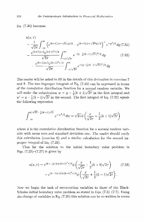
124 An Undergraduate Introduction to Financial Mathematics
Eq. (7.30) becomes
U(X,T)
= _ L _ / Lik+Vix+V^y)^ _ e(k-l)(x+V2^y)/2y e-y2/2 dy,731^
e e f e-(y-H^)v^r/2dy (7-32) 27T J-x/\
Jk-l)x/2Jk-l)2T/4 roo
V27T J-x/V2^
The reader will be asked to fill in the details of this derivation in exercises 7
and 8. The two improper integrals of Eq. (7.32) can be expressed in terms
of the cumulative distribution function for a normal random variable. We
will make the substitution w = y — |(fc + 1 ) \ / 2 T in the first integral and
w' = y — |(fc — l ) \ / 2 r in the second. The first integral of Eq. (7.32) equals
the following expression
fx/VZF+Hk+VV^ / T 1 , ' / e~w/2 dw = V2^(f> [—= + -{k + l)\^
J-oo V V 2 T 2
where 4> is the cumulative distribution function for a normal random vari
able with mean zero and s tandard deviation one. The reader should verify
this calculation (exercise 9) and a similar calculation for the second im
proper integral of Eq. (7.32).
Thus far the solution to the initial boundary value problem in
Eqs. (7.25)-(7.27) is given by
u(x, r ) = e(>=+iW2+(M-i)2T/40 (* + hk + 1 ) V ^ A ( 7 3 3 )
V V 2r 2 J
s ( / c - lW2+( / c - l )V4 0 (* + 1 {k _ 1)y/£f\ .
Now we begin the task of reconverting variables to those of the Black-
Scholes initial boundary value problem as stated in Eqs. (7.5)-(7.7). Using
the change of variables in Eq. (7.20) this solution can be re-written in terms
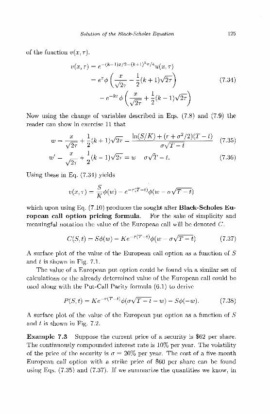
Solution of the Black-Scholes Equation 125
of the function V(X,T).
V(X,T) = e - ( i - l ) x / 2 - ( f c + l ) ' x / 4 t ( ( l i T )
= (vi + ^ + 1 ) V 5 7 ) - " * * ( ^ + 5 ( * - 1 ) , / 5 f
(7.34)
Now using the change of variables described in Eqs. (7.8) and (7.9) the reader can show in exercise 11 that
^ J L . l l U D V g . ^ ' ^ ^ - " (7.35)
+ l{k- 1)V2T = W- cry/T - t. (7.36) / x
w V^ 2
Using these in Eq. (7.34) yields
V(X,T) = ^4>{w) - e _ r ( T - ' V ( ' « " <ry/T^t)
which upon using Eq. (7.10) produces the sought after Black-Scholes European call option pricing formula. For the sake of simplicity and meaningful notation the value of the European call will be denoted C.
C{S, t) = S<j>{w) - Ke-r(T-t](t>{w - aVT^t) (7.37)
A surface plot of the value of the European call option as a function of S and t is shown in Fig. 7.1.
The value of a European put option could be found via a similar set of calculations or the already determined value of the European call could be used along with the Put-Call Parity formula (6.1) to derive
P(S, t) = Ke-^-^^oy/T - t - w) - S<t>{-w). (7.38)
A surface plot of the value of the European put option as a function of S and t is shown in Fig. 7.2.
Example 7.3 Suppose the current price of a security is $62 per share. The continuously compounded interest rate is 10% per year. The volatility of the price of the security is a = 20% per year. The cost of a five-month European call option with a strike price of $60 per share can be found using Eqs. (7.35) and (7.37). If we summarize the quantities we know, in
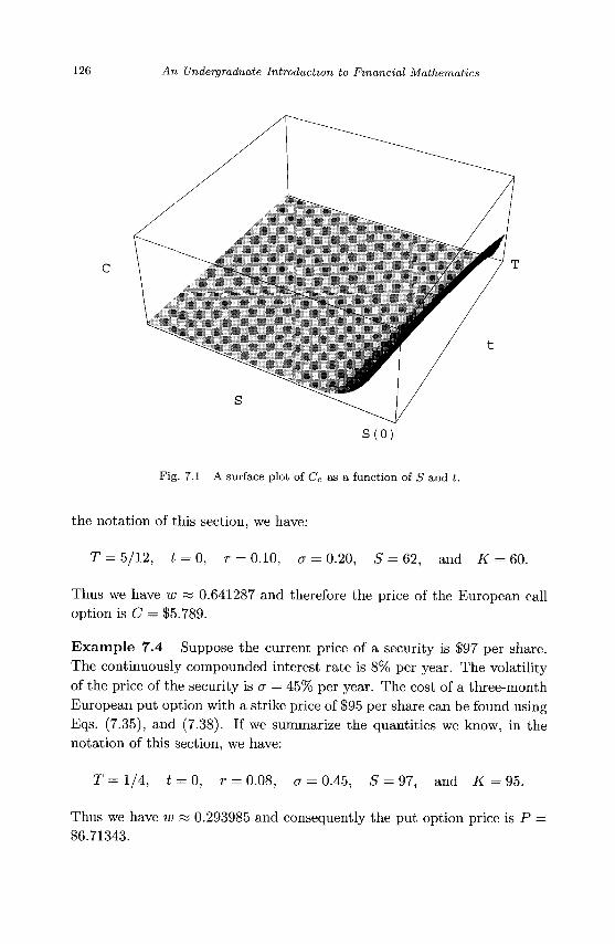
126 An Undergraduate Introduction to Financial Mathematics
S ( 0 )
Fig. 7.1 A surface plot of Ce as a function of S and t.
the notation of this section, we have:
T = 5/12, £ = 0, r = 0.10, a = 0.20, 5 = 62, and K = 60.
Thus we have w « 0.641287 and therefore the price of the European call option is C = $5,789.
Example 7.4 Suppose the current price of a security is $97 per share. The continuously compounded interest rate is 8% per year. The volatility of the price of the security is a = 45% per year. The cost of a three-month European put option with a strike price of $95 per share can be found using Eqs. (7.35), and (7.38). If we summarize the quantities we know, in the notation of this section, we have:
T = l / 4 , t = 0, r = 0.08, a = 0.45, S = 97, and K = 95.
Thus we have w as 0.293985 and consequently the put option price is P = $6.71343.
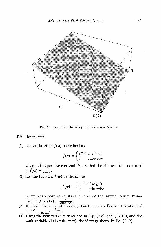
Solution of the Black-Scholes Equation 127
S ( 0 )
Fig. 7.2 A surface plot of Pe as a function of S and t.
7.5 Exercises
(1) Let the function f(x) be defined as
" e~ax if x > 0 1 0 otherwise
where a is a positive constant. Show that the Fourier Transform of /
(2) Let the function f(w) be defined as
if x f e~aw if w > 0 / ( to) = < „
[0 otherwise
where a is a positive constant. Show that the inverse Fourier Transform of f is f(x) = 0 , 1 • ^.
J J \ I 27r(a—ix)
(3) If o is a positive constant verify that the inverse Fourier Transform of
e-<™2 is -4=e-x 2 /4<\ (4) Using the new variables described in Eqs. (7.8), (7.9), (7.10), and the
multivariable chain rule, verify the identity shown in Eq. (7.12).
128 An Undergraduate Introduction to Financial Mathematics
(5) Using the new variables described in Eqs. (7.8), (7.9), (7.10), the expression for Fs shown in (7.11), and the multivariable chain rule, verify the identity shown in Eq. (7.13).
(6) Verify that the Black-Scholes partial differential Eq. (7.5) can be simplified to the form shown in Eq. (7.14) by using the variables described in (7.8), (7.9), and (7.10) and the partial derivatives found in (7.11), (7.12), and (7.13).
(7) Verify that the expression
/e(fc+i)(x+- /5Fy)/2 _ Jk-l)(x+V2^y)/2~y2/2^ —N +
e(K-i)(x-t-v<tTy)/ze~y I*^J2T
is non-zero whenever y > —X/\/2T.
(8) Use completion of the square in the exponents of the integrand in Eq. (7.31) to derive Eq. (7.32).
(9) Using the change of variable w = — y + \(k + l ) \ /2 r in the first improper integral of Eq. (7.32) verify that
1 r°° 1 ' e-(y-i(k+l)V^)2f2dy
'2n J~X/V2
e 2 dw
(x/V^+Uk + l)^
where (j> is the cumulative distribution function for a normal random variable with mean zero and standard deviation one.
(10) Using the change of variable w' = — y + \{k — l)v /2r in the second improper integral of Eq. (7.32) verify that
1 ' "" - ( y - i ( f e - l ) v ^ ) 2 / 2 e-(y-i(K-i-)V2T)-/-z dy
TO'2
e 2" dw'
>2-K J-x/y/2-
(x/V2r+^(k- 1)V2T
where <f> is the cumulative distribution function for a normal random variable with mean zero and standard deviation one.
Solution of the Black-Scholes Equation 129
(11) Verify using the change of variable formulas in Eqs. (7.8) and (7.9) and the fact that k = 2r/a2 that
X/^?+1-(k + l)^ = HS/K)HrJ^/2)(T-t)
X/^P+1-(k-l)^= MS/K) + (r+f/2)(T-t) _aV¥-t
2 <j\JT — t
(12) What is the price of a European call option on a stock when the stock price is $52, the strike price is $50, the interest rate is 12%, the stock's volatility is 30%, and the exercise time is three months?
(13) What is the price of a European put option on a stock when the stock price is $69, the strike price is $70, the interest rate is 5%, the stock's volatility is 35%, and the exercise time is six months?
(14) A European call option on a stock has a market value of $2.50. The stock price is $15, the strike price is $13, the interest rate is 5%, and the exercise time is three months. What is the volatility of the stock?
(15) Show by differentiation and substitution in Eq. (7.5) that the price of the security itself, i.e. f(S,t) = S solves the Black-Scholes equation.

This page is intentionally left blank
Chapter 8
Derivatives of Black-Scholes Option Prices
Now that the solution to the Black-Scholes equation is known we can investigate the sensitivity of the solution to changes in the independent variables. Knowledge of these sensitivities allows a portfolio manager to minimize changes in the value of a portfolio when underlying variables such as the risk-free interest rate change. The material of the present chapter will be use extensively in Chapter 9. An understanding of the sensitivity of an option's value to changes in its independent variables will also provide a new way of interpreting the Black-Scholes equation itself.
To mathematicians the word derivative means an instantaneous rate of change in a quantity. To a quantitative analyst a derivative is a financial entity whose value is derived from the value of some underlying asset. Hence a European call option is a derivative who value is a function of (among other things) the value of the security underlying the option. In this chapter we explore derivatives from the mathematician's perspective. In the Chapter 9 we will use these derivatives in the manner of a quantitative analyst. Members of the quantitative financial profession refer to the subject matter of this chapter as the "Greeks" since a Greek letter is used to name each derivative (except for one which we will meet in due time).
8.1 Theta
The quantity 0 is defined to be the rate of change of the value of an option with respect to t. We will calculate 8 for the European call and put options derived in Chapter 7. Since the valuation of European-style options depends heavily on the cumulative distribution function of the standard normal random variable and a composite variable w, we will begin by investigating their partial derivatives. The derivative with respect to t of quantity w
131
132 An Undergraduate Introduction to Financial Mathematics
defined in Eq. (7.35) is given by
dw 1 (HS/K) \
dt -2aVT=t{ T-t T ° /2J- ( 8-1 }
By the Fundamental Theorem of Calculus [Smith and Minton (2002), Chap. 4] the cumulative distribution function for the standard normal distribution has derivative
tf{x) = ^Le"*2 /2 . (8.2) \f2-K
Hence using the Chain Rule [Stewart (1999), Chap. 3] for derivatives we can see that the time rate of change in the value of a European call option (defined in Eq. (7.37)) is
= S<f>'(w)^ - Ke^-V (r<Kw - ay/T^i) dt
dw + (j)1(w - aVT - t)
_dt 2^/T^t dw ~dt
= (s</>'(w) " Ke-'V-'Wiw ~ (ry/T=tj\
- Ke~r(-T~V (rcj>{w - ay/Y^t) + ° </>'\w - ay/T=t)\
_ S<//(w) - K e - r < r - ' V ( w - aVT^t) f\n{S/K) _ 2
2aVT^t \ T-t T a '
- Ke-r(T-t) (r<j){w - av'T - t) + ° $ {w - ay/T - tU
5 e - - 2 /2 _ Ke-r(T-t)-(W-*VT=tf/2 (MSIK) 2 ,„ 0 C = . —^-i-—- - r - a2, 2
2a^/2Tr(T -1) \ T-t '
( , np-(w-ajT=if / 2 \
-^-'>{r^-,VT^)+ V M r _ ( ) j (8.3) To take an example, consider a European call option on a stock whose current price is $250. The strike price is $245, the annual risk-free interest rate is 2.5%, the volatility of the stock price is 20%, and the strike time is four months. Thus substituting S = 250, K = 245, r = 0.025, a = 0.20, T = 1/3, and t = 0 into Eq. (8.3) produces
6 = — = -19.9836. at
Derivatives of Black-Scholes Option Prices 133
The case that 0 is negative for an option is typical since options lose value as the expiry date approaches.
The calculation of 0 for a European put option is carried out in a similar fashion to that for the call option. The reader will be asked to provide the details of the following derivation.
dP &P = ^ - (8.4)
dP
Se-w2/i f\n{S/K)
2aV'27r(T - t ) \ T-t
+ Kre
Ke~
-^'-^{ay/T-t-•r(T-t)-(w~aVT^t)2 / :
2a^2n(T -t)
- r -
w)
- ( '
- -72)
n(S/K) T-t
r + a2/2) (8.5)
Equation (8.5) will be put to use in the following example. Consider a European put option on a stock whose current price is $325. The strike price is $330, the annual risk-free interest rate is 3.5%, the volatility of the stock price is 27%, and the strike time is three months. Thus substituting S = 325, K = 330, r = 0.035, a = 0.27, T = 1/4, and t = 0 into Eq. (8.5) produces
dP e = — = -28.7484.
dt
The derivative 0 , is unique among the derivatives covered in this chapter. The passage of time t, is the only non-stochastic variable among the list of independent variables upon which C or P depend.
8.2 Delta
The value of an option is also sensitive to changes in the price of the underlying stock. This rate of change is called Delta, A. The astute reader may recall that A was introduced in Sec. 6.3 during the derivation of the Black-Scholes partial differential equation. Delta was used to eliminate a stochastic term from Eq. (6.12). The clever choice of A left us with a deterministic partial differential equation to solve rather than a stochastic differential equation. The starting point for deriving A is again Eq. (7.37).
| | = </,(w) + (V(W) - Ke-^T^4>'(W - aVT^t)) g (8.6)
134 An Undergraduate Introduction to Financial Mathematics
We can make use of Eq. (8.2) and the following result.
dw 1
dS aSVT^t
Substituting Eqs. (8.2) and (8.7) into Eq. (8.6) produces
dC ,, s (Se~w2'2 x e - ( ^ ) e - ( » - - V T = t ) 2 / 2 \ ! (w) +
J.7)
dS ^v \ V^TT V2TT J aSVT^t
ay/2n(T - t)
e-^ 2 /2
( w ) + " I 1 _ 11^ p - ( ^ (T- ( ) -2™VT=t ) /2
M + av/2n(T - t)
1 _ J C e - r ( T - * ) c _ ( c 7 2 ( T _ t ) _ 2 ( r + ( T 2 / 2 ) ( r _ 0 + 2 1 n ( J f / i g ) ) / 2 \
= fty,) + f ( 1 _ ^ £ _ er(T-t)+ln(S/Ar)
= 0(u)) + f^2 (i - EeHs/K)\ ay/27r(T - t ) \ S J
e-w2/2
= </>{w) (8.8)
We can put this formula to use in the following example. Suppose the price of a security is $100, the risk-free interest rate is 4% per annum, the annual volatility of the stock price is 23%, the strike price is $110, and the strike time is 6 months. Under these conditions w = —0.381747 and
dC A c = — = 0.351325.
Delta for a European put option could be calculated directly from the definition for P; however, the Put-Call parity formula (Eq. (6.1)) provides a convenient shortcut.
3P_ _ ac ds + ~ ds
dP Ap = ~dS= ^w) " * ( 8 ' 9 )
Derivatives of Black-Scholes Option Prices 135
Thus using the same parameter values as in the previous example,
§ ^ = 0.351325 - 1 = -0.648675. Co
So as the European call option increases in value with an increase in the value of the underlying security, the put option decreases in value.
8.3 G a m m a
The g a m m a T, of an option or collection of options is defined to be the second derivative of the option with respect to S, the price of the underlying security. Hence T is the partial derivative of A with respect to S. Thus for a European call option T is
d2C d fdC dS2 dS \ dS
d ds Mw)) (using Eq. (8.8))
w2/2 / j
/2~7r \aSVT-t p-w>/2
crSy27r(T - 1 )
We can readily see from Eq. (8.9) that
(using exercise 4)
(8.10)
d2P _d2C e~w^2
~ dS2 ~ dS2 - aSy/2n(T-t)' ( 8 " U )
If all independent variables are held fixed except for S, then T measures the concavity of the value of the option as a function of S. Suppose we consider a European call option on a security whose value is $295. The strike price is $290, the annual risk-free interest rate is 4.25%, the volatility of the security is 25% per annum, and the expiry date is two months. We can calculate the price of the option, its A, and its T as follows.
C = 15.7173, A c = 0.613297, T = 0.0127122
Thus the value of the option will increase with the price of the underlying security at an increasing rate. As the price of the security increases, the
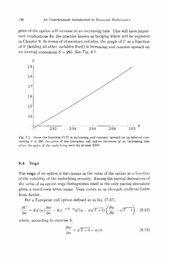
136 An Undergraduate Introduction to Financial Mathematics
price of the option will increase at an increasing rate. This will have important implications for the practice known as hedging which will be explored in Chapter 9. In terms of elementary calculus, the graph of C as a function of S (holding all other variables fixed) is increasing and concave upward on an interval containing S = 295. See Fig. 8.1.
C
191
17
16
15
14
292 294 296 298 300
Fig. 8.1 Since the function C(S) is increasing and concave upward on an interval containing S = 295 the price of the European call option increases at an increasing rate when the price of the underlying security is near $295.
8.4 Vega
The vega of an option is the change in the value of the option as a function of the volatility of the underlying security. Among the partial derivatives of the value of an option vega distinguishes itself as the only partial derivative given a non-Greek letter name. Vega comes to us through medieval Latin from Arabic.
For a European call option defined as in Eq. (7.37),
dC_ . dw S(j)'{w)— - Ke-'W-Qfiiw - aVT~^t)
da \
f dw ~da~ VT-t
where, according to exercise 8,
dw ~do~
sjT-t - w/a.
.12)
(8.13)
Derivatives of Black-Scholes Option Prices 137
Substituting Eq. (8.13) into Eq. (8.12) produces
dC
s<f>'(w) (yr=i- ^) + Ke-^^H'iw -aVr~i) (^)
Sy/T=i(l>'(w) - - (s</>'{w) - Ke-^-^fiiw - ay/T^t)^
Sy/T=i<l>'(w) - ~^= (Se~w2/2 - Ke-r(T~t)e-(w-aVT=if/2\ ay/2TT \ '
Sy/T - t(j>'(w)
w ay/^n
e-w2l2 (g __ Ke-r(T-t)+waVT=i-a2(T-t)/2
W = SVT=i<l>'(w) - -^—e-w'2
X (S - ^ e-r(T-i)+ln( ,S/ . ff) + ( r+ C T2 /2 ) (T- t ) -<x 2 (T- t ) /2 \
SVT~t<P'(w) - ^ ^ e - 2 / 2 fs _ KeHs/K)\
sVr^tcp'(w) ~ -^—e-w2i2{s - s)
a\/2TT
SVT-t _w2/2 /2TT
e~w !1 (8.14)
Note that the value of the European call option increases with increasing volatility in the underlying security. It is easily seen from the Put-Call Parity Formula (Eq. (6.1)) that
dP Sy/T=t _w2/2
da V27T e-w l\ (8.15)
in other words the rate of change in the value of a European put option with respect to volatility is the same as the rate of change in the value of the corresponding European call option with respect to volatility. Thus we may unambiguously define vega for a European style option to be
v=5VTEte_„,V2_ (816) V27T
Thus the vega for a European style option (either call or put) on a security who current value is $160, whose strike price is $150, and whose expiry
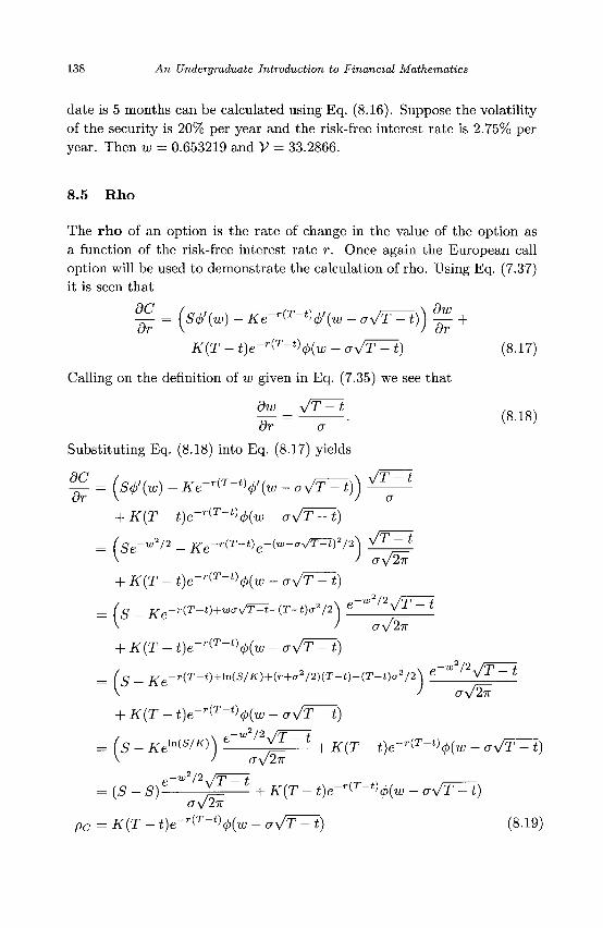
138 An Undergraduate Introduction to Financial Mathematics
date is 5 months can be calculated using Eq. (8.16). Suppose the volatility of the security is 20% per year and the risk-free interest rate is 2.75% per year. Then w = 0.653219 and V = 33.2866.
8.5 Rho
The rho of an option is the rate of change in the value of the option as a function of the risk-free interest rate r. Once again the European call option will be used to demonstrate the calculation of rho. Using Eq. (7.37) it is seen that
^ = ( W H - Ke-^-^'iw - aVT^t)) ^ +
K(T - £)e- r ( T-*V(w - aVT^t) (8.17)
Calling on the definition of w given in Eq. (7.35) we see that
dw _ y/T^t dr a
Substituting Eq. (8.18) into Eq. (8.17) yields
(8.18)
d-§- = (S<p'(w) - Ke-^T-^4>'{w - vy/T=ij) ^ - ^ or V / a
+ K{T - t)e- r ( T-*V(™ - aVT^t)
x/T^t (Se-w2'2 - Ke-r(T-t)e-{w-*VT=lY/2\ y_ V / ay/2-K
+ K(T - i ) e - r ( T - t ) 0 ( w - aVT^t)
(s - Ke~r{T~t)+waVT^i'{T''t)a2/2) e W /2^T l
V / aV2n + K(T - t )e- r ( T -*V(w - aVT - t)
(S - Ke-HT-t)+HS/K) + (r+*2/V(T-t)-(T-t)a2/2\ e~W *\/T-t
\ ) aV2n
+ K(T - i)e- r (T- t )</»(^ - <ry/T=t)
(S - Kel^s/KA C~W ' 2 ^ r ~ t + K(T - t)e-^T-V<t>{w - aVT^t) V / ay/lit
„-W2/2/rp _ J.
(S _ s)- ^ ^ + K(T - t)e-^T-^4>{w - *y/T=i) O\J2-K
pc = KiT - i)e-r(T-t}4>(w - oy/T^t) (8.19)
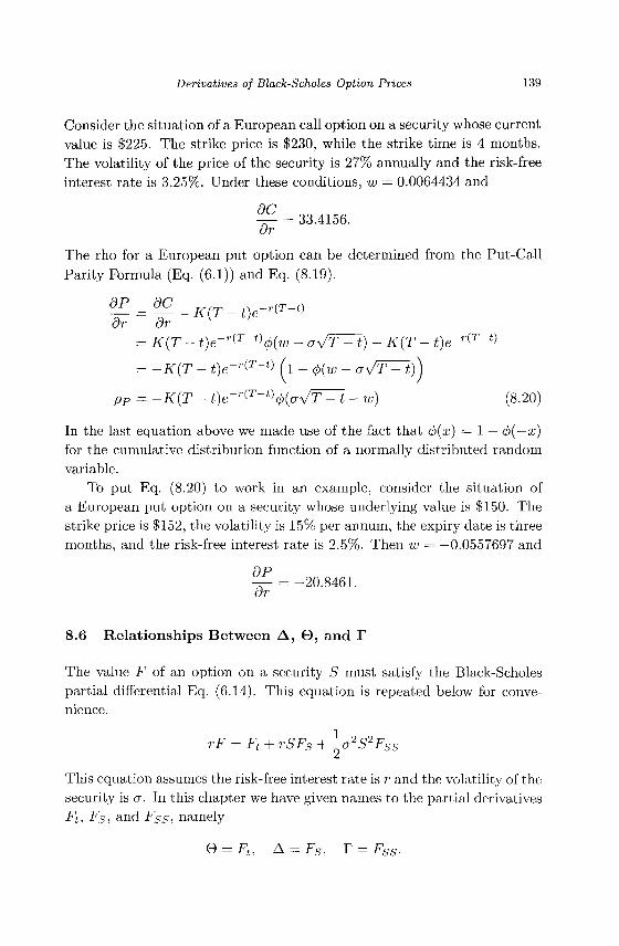
Derivatives of Black-Scholes Option Prices 139
Consider the situation of a European call option on a security whose current value is $225. The strike price is $230, while the strike time is 4 months. The volatility of the price of the security is 27% annually and the risk-free interest rate is 3.25%. Under these conditions, w = 0.0064434 and
^ = 33.4156. or
The rho for a European put option can be determined from the Put-Call Parity Formula (Eq. (6.1)) and Eq. (8.19).
= K(T - t)e-<T~^4>{w - aVT^t) - K{T - t)e~r(T~^
= -K(T - t ) e - r ( r - ' ) ( l - <t>(w - aVT^t)^j
pP = -K{T - i ) e - r ( T - t V(<r \ /T - t - w) (8.20)
In the last equation above we made use of the fact that <f>(x) = 1 — 4>(—x) for the cumulative distribution function of a normally distributed random variable.
To put Eq. (8.20) to work in an example, consider the situation of a European put option on a security whose underlying value is $150. The strike price is $152, the volatility is 15% per annum, the expiry date is three months, and the risk-free interest rate is 2.5%. Then w = —0.0557697 and
dP -—- = -20.8461. or
8.6 Relationships Between A, 0 , and T
The value F of an option on a security S must satisfy the Black-Scholes partial differential Eq. (6.14). This equation is repeated below for convenience.
rF = Ft + rSFs + -<J2S2FSS
This equation assumes the risk-free interest rate is r and the volatility of the security is a. In this chapter we have given names to the partial derivatives Ft, Fs, and FSs, namely
e = Ft, A = FS, ss-
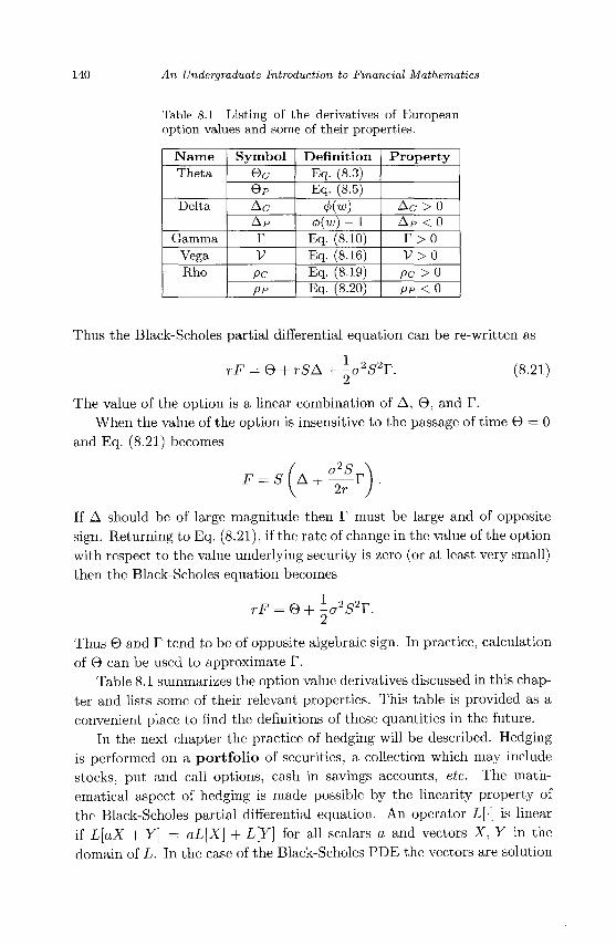
140 An Undergraduate Introduction to Financial Mathematics
Table 8.1 Listing of the derivatives of European option values and some of their properties.
N a m e Theta
Delta
Gamma Vega Rho
Symbol
e c eP A c
A P
r V
PC
PP
Definition Eq. (8.3) Eq. (8.5)
<p(w) 4>(w) - 1
Eq. (8.10) Eq. (8.16) Eq. (8.19) Eq. (8.20)
Property
A c > 0 A P < 0
r > o V > 0
pc > 0 pp < 0
Thus the Black-Scholes part ial differential equation can be re-written as
rF = 0 + rSA + )-a2S2T. (8.21)
The value of the option is a linear combination of A, 0 , and F.
When the value of the option is insensitive to the passage of t ime 0 = 0
and Eq. (8.21) becomes
If A should be of large magnitude then T must be large and of opposite
sign. Returning to Eq. (8.21), if the rate of change in the value of the option
with respect to the value underlying security is zero (or at least very small)
then the Black-Scholes equation becomes
rF = e+^a2S2T.
Thus 0 and T tend to be of opposite algebraic sign. In practice, calculation
of 0 can be used to approximate F.
Table 8.1 summarizes the option value derivatives discussed in this chap
ter and lists some of their relevant properties. This table is provided as a
convenient place to find the definitions of these quantities in the future.
In the next chapter the practice of hedging will be described. Hedging
is performed on a port fo l io of securities, a collection which may include
stocks, put and call options, cash in savings accounts, etc. The math
ematical aspect of hedging is made possible by the linearity property of
the Black-Scholes part ial differential equation. An operator L[-] is linear
if L[aX + Y] = aL[X] + L[Y] for all scalars a and vectors X, Y in the
domain of L. In the case of the Black-Scholes P D E the vectors are solution
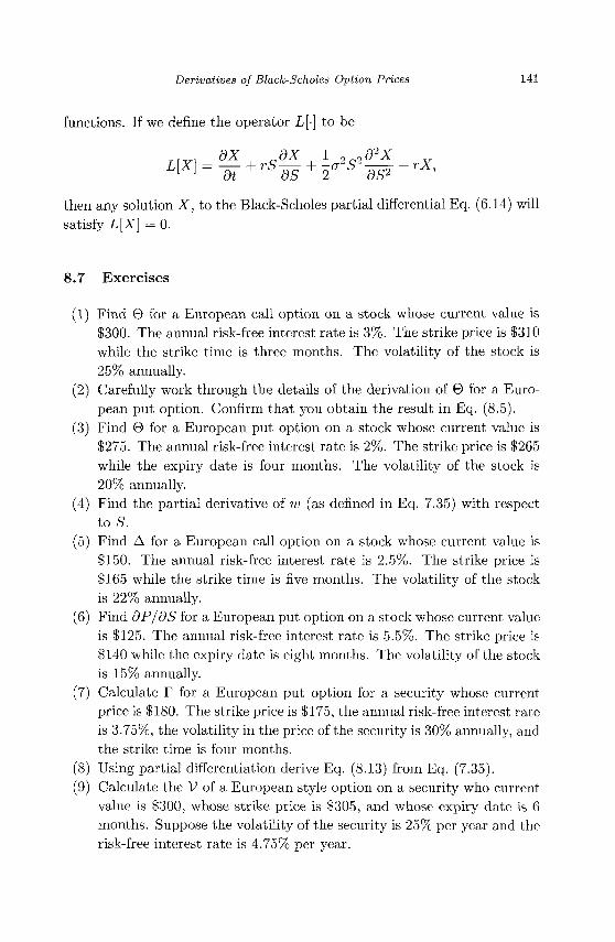
Derivatives of Black-Scholes Option Prices 141
functions. If we define the operator L[-] to be
r r x r l dX adX 1 2a2d2X
L^ = iH+rSM+rs^-rX> then any solution X, to the Black-Scholes partial differential Eq. (6.14) will satisfy L[X] = 0.
8.7 Exercises
(1) Find 0 for a European call option on a stock whose current value is $300. The annual risk-free interest rate is 3%. The strike price is $310 while the strike time is three months. The volatility of the stock is 25% annually.
(2) Carefully work through the details of the derivation of 0 for a European put option. Confirm that you obtain the result in Eq. (8.5).
(3) Find 0 for a European put option on a stock whose current value is $275. The annual risk-free interest rate is 2%. The strike price is $265 while the expiry date is four months. The volatility of the stock is 20% annually.
(4) Find the partial derivative of w (as defined in Eq. 7.35) with respect toS.
(5) Find A for a European call option on a stock whose current value is $150. The annual risk-free interest rate is 2.5%. The strike price is $165 while the strike time is five months. The volatility of the stock is 22% annually.
(6) Find dP/dS for a European put option on a stock whose current value is $125. The annual risk-free interest rate is 5.5%. The strike price is $140 while the expiry date is eight months. The volatility of the stock is 15% annually.
(7) Calculate T for a European put option for a security whose current price is $180. The strike price is $175, the annual risk-free interest rate is 3.75%, the volatility in the price of the security is 30% annually, and the strike time is four months.
(8) Using partial differentiation derive Eq. (8.13) from Eq. (7.35). (9) Calculate the V of a European style option on a security who current
value is $300, whose strike price is $305, and whose expiry date is 6 months. Suppose the volatility of the security is 25% per year and the risk-free interest rate is 4.75% per year.
142 An Undergraduate Introduction to Financial Mathematics
(10) Calculate the rho of a European style put option on a security who current value is $270, whose strike price is $272, and whose strike time is 2 months. Suppose the volatility of the security is 15% per year and the risk-free interest rate is 3.75% per year.
(11) Calculate the rho of a European style call option on a security who current value is $305, whose strike price is $325, and whose expiry date is 4 months. Suppose the volatility of the security is 35% per year and the risk-free interest rate is 2.55% per year.
Chapter 9
Hedging
Hedging is the practice of making a portfolio of investments less sensitive to changes in market variables such as the prices of securities and interest rates. If F(S, t) is a solution to the Black-Scholes partial differential Eq. (6.14), the quantity A = Fs is central to hedging a portfolio. In fact this same quantity A, was used to derive the Black-Scholes PDE. The Black-Scholes equation can be thought of as the statement that when A is zero, the rate of return from a portfolio consisting of ownership of the underlying security and sale of the option (or the opposite positions) should be the same as the rate of return from the risk-free interest rate on the same net amount of cash.
In Chapter 8 the partial derivatives of the values of European put and call options were calculated. In this chapter they will be used to hedge portfolios of investments.
9.1 General Principles
Before launching into a discussion of hedging, let us pause and recall what happens when a one entity (say, a bank) sells a call option on a stock to another entity (say, an investor). The bank has promised the investor that they will be able to purchase the stock at a predetermined price (the strike price), at a predetermined time (the expiry date) in the future. The stock must be available to the investor at the strike price even if the market value of the stock exceeds the strike price. The bank is in a favorable position if, at the strike time, the market price of the stock is below the strike price set when the call option was sold to the investor. In this case the call option will not be exercised and the bank keeps the money it received when it sold the option. Conversely, if the market price of the stock exceeds the strike
143
144 An Undergraduate Introduction to Financial Mathematics
price of the option, the bank must ensure the investor can find a seller of the stock who will agree to accept the strike price. One way to accomplish this would be for the bank itself to be the seller to the investor.
Consider this strategy: the bank creates a European call option on a stock whose current price is $50 while the strike price is $52, the risk-free interest rate is 2.5% per annum, the expiry date is four months, and the volatility of the stock price is 22.5% per annum. According to the Black-Scholes option pricing formula, the value of this European call option is $1.91965. So that we deal with whole numbers, suppose an investor purchases one million of these call options. The bank accepts revenue equal to $1,919,650. The bank could wait until the expiry date to purchase the one million shares of the stock, or they could purchase one million shares at the time the investor bought the million call options. Suppose the bank takes the latter course, they will expend $50M, considerably more than the revenue generated by the sale of the call options. If S represents the price per share of the stock at the strike time then the net revenue generated by the transaction obeys the formula
1919650+ (min{52, S'}e-0 0 2 5 / 3 - 50) • 106.
Notice that the present value of the stock price must be incorporated rather than just S. The reader can check that when S « 48.4827 the net expenditure is zero. Figure 9.1 shows if the stock is below that price the bank loses money (at S = 46 the loss comes to more than $2.4M), and if the stock price is higher the bank profits (at S = 52 the profit nearly $3.5M). Since the strike price is $52, the maximum net revenue for the bank occurs at that price.
Another option for the bank is to purchase the stock at the strike time and instantaneously sell it to the investor at the strike price. In this scenario the net revenue generated by this sequence of transactions is
1919650 + min{0,52 - 5 } e - ° 0 2 5 / 3 • 106.
The net revenue is zero when S is approximately $53.9357. As long as the stock price remains below the strike price the bank keeps its revenue from the sale of the options. However the bank's losses could be dramatic when the price of the stock rises before the expiry date. At a price of $56 per share the bank's net loss would be approximately $2.0M. Figure 9.2 illustrates the profit or loss to the seller of the European call option.
Neither of these schemes are practical for hedging portfolios in the fi-
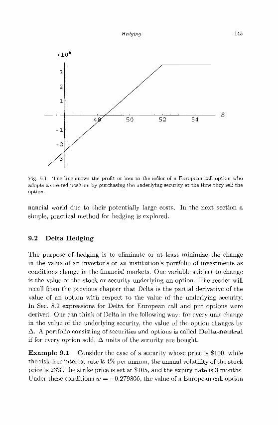
Hedging 145
, 1 0 b
Fig. 9.1 The line shows the profit or loss to the seller of a European call option who adopts a covered position by purchasing the underlying security at the time they sell the option.
nancial world due to their potentially large costs. In the next section a simple, practical method for hedging is explored.
9.2 Delta Hedging
The purpose of hedging is to eliminate or at least minimize the change in the value of an investor's or an institution's portfolio of investments as conditions change in the financial markets. One variable subject to change is the value of the stock or security underlying an option. The reader will recall from the previous chapter that Delta is the partial derivative of the value of an option with respect to the value of the underlying security. In Sec. 8.2 expressions for Delta for European call and put options were derived. One can think of Delta in the following way: for every unit change in the value of the underlying security, the value of the option changes by A. A portfolio consisting of securities and options is called Delta-neutral if for every option sold, A units of the security are bought.
Example 9.1 Consider the case of a security whose price is $100, while the risk-free interest rate is 4% per annum, the annual volatility of the stock price is 23%, the strike price is set at $105, and the expiry date is 3 months. Under these conditions w = —0.279806, the value of a European call option
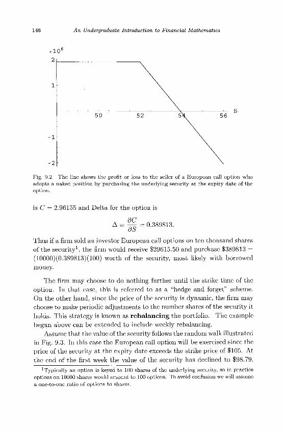
146 An Undergraduate Introduction to Financial Mathematics
, 1 0 °
Fig. 9.2 The line shows the profit or loss to the seller of a European call option who adopts a naked position by purchasing the underlying security at the expiry date of the option.
is C = 2.96155 and Delta for the option is
dC A = — = 0.389813.
ob
Thus if a firm sold an investor European call options on ten thousand shares of the security1, the firm would receive $29615.50 and purchase $389813 = (10000)(0.389813)(100) worth of the security, most likely with borrowed money.
The firm may choose to do nothing further until the strike time of the option. In that case, this is referred to as a "hedge and forget" scheme. On the other hand, since the price of the security is dynamic, the firm may choose to make periodic adjustments to the number shares of the security it holds. This strategy is known as rebalancing the portfolio. The example begun above can be extended to include weekly rebalancing.
Assume that the value of the security follows the random walk illustrated in Fig. 9.3. In this case the European call option will be exercised since the price of the security at the expiry date exceeds the strike price of $105. At the end of the first week the value of the security has declined to $98.79.
1 Typically an option is keyed to 100 shares of the underlying security, so in practice options on 10000 shares would amount to 100 options. To avoid confusion we will assume a one-to-one ratio of options to shares.
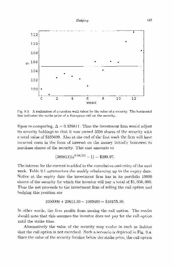
Hedging 147
0 2 4 6 8 1 0 1 2 w e e k
Fig. 9.3 A realization of a random walk taken by the value of a security. The horizontal line indicates the strike price of a European call on the security.
Upon re-computing, A = 0.339811. Thus the investment firm would adjust its security holdings so that it now owned 3398 shares of the security with a total value of $335699. Also at the end of the first week the firm will have incurred costs in the form of interest on the money initially borrowed to purchase shares of the security. This cost amounts to
(389813)(e004/52 - 1) = $299.97.
The interest for the current is added to the cumulative cost entry of the next week. Table 9.1 summarizes the weekly rebalancing up to the expiry date. Notice at the expiry date the investment firm has in its portfolio 10000 shares of the security for which the investor will pay a total of $1, 050,000. Thus the net proceeds to the investment firm of selling the call option and hedging this position are
1050000 + 29615.50 - 1069460 = $10155.50.
In other words, the firm profits from issuing the call option. The reader should note that this assumes the investor does not pay for the call option until the strike time.
Alternatively the value of the security may evolve in such as fashion that the call option is not exercised. Such a scenario is depicted in Fig. 9.4. Since the value of the security finishes below the strike price, the call option
112
110
108
w 106
104
102
100
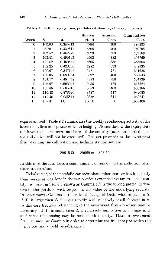
148 An Undergraduate Introduction to Financial Mathematics
Table 9.1 Delta hedging using portfolio rebalancing at weekly intervals.
Week 0 1 2 3 4 5 6 7 8 9 10 11 12 13
S 100.00
98.79
102.52
103.41
102.82
102.25
100.67
106.05
104.17
106.08
105.86
110.40
112.46
108.47
A
0.389813
0.339811
0.462922
0.490192
0.460541
0.428236
0.347145
0.589204
0.491348
0.595047
0.585915
0.878690
0.985811
1.0
Shares
Held
3898
3398
4629
4902
4605
4282
3471
5892
4913
5950
5859
8787
9858
10000
Interest
Cost
300 262 359 382 358 333 271 468 390 475 468 717 811 0
Cumulative
Cost
389800
340705
467169
495760
465604
432935
351625
608643
507129
617524
608366
932085
1053247
1069460
expires unused. Table 9.2 summarizes the weekly rebalancing activity of the investment firm as it practices Delta hedging. Notice that at the expiry date the investment firm owns no shares of the security (none are needed since the call option will not be exercised). The net proceeds to the investment firm of selling the call option and hedging its position are
29615.50 - 29669 = -$53.50.
In this case the firm loses a small amount of money on the collection of all these transactions.
Rebalancing of the portfolio can take place either more or less frequently than weekly as was done in the two previous extended examples. The quantity discussed in Sec. 8.3 known as Gamma (r) is the second partial derivative of the portfolio with respect to the value of the underlying security. In other words Gamma is the rate of change of Delta with respect to S. If |F| is large then A changes rapidly with relatively small changes in S. In this case frequent rebalancing of the investment firm's position may be necessary. If |T| is small then A is relatively insensitive to changes in S and hence rebalancing may be needed infrequently. Thus an investment firm can monitor Gamma in order to determine the frequency at which the firm's position should be rebalanced.
Hedging 149
Fig. 9.4 Another realization of a random walk taken by the value of a security. The horizontal line indicates the strike price of a European call on the security.
9.3 Delta Neutral Portfolios
In exercise 15 of Chapter 7 the reader was asked to verify that a stock or security itself satisfies the Black-Scholes PDE (6.14). Now suppose that a portfolio consists of a linear combination of options and shares of the underlying security. The portfolio contains a short position in a European call option and a long position in the security (hedged appropriately as described in the previous section). Thus the net value V of the portfolio is
V=C-AS=C dC_
as s, (9.1) So
where So is the price of the security at the time the hedge is created. The quantity V satisfies the Black-Scholes equation since C and S separately do, and the equation is linear. Thus it reasonable to contemplate Delta for the portfolio. The partial derivative of the entire portfolio with respect to S represents the sensitivity of the value of the portfolio to changes in S. Differentiating both sides of Eq. (9.1) with respect to S produces
dV OS
dC ~dS So
This quantity equals zero whenever S = SQ (for example at the moment the hedge is set up) and remains very close to zero so long as S is near So- For
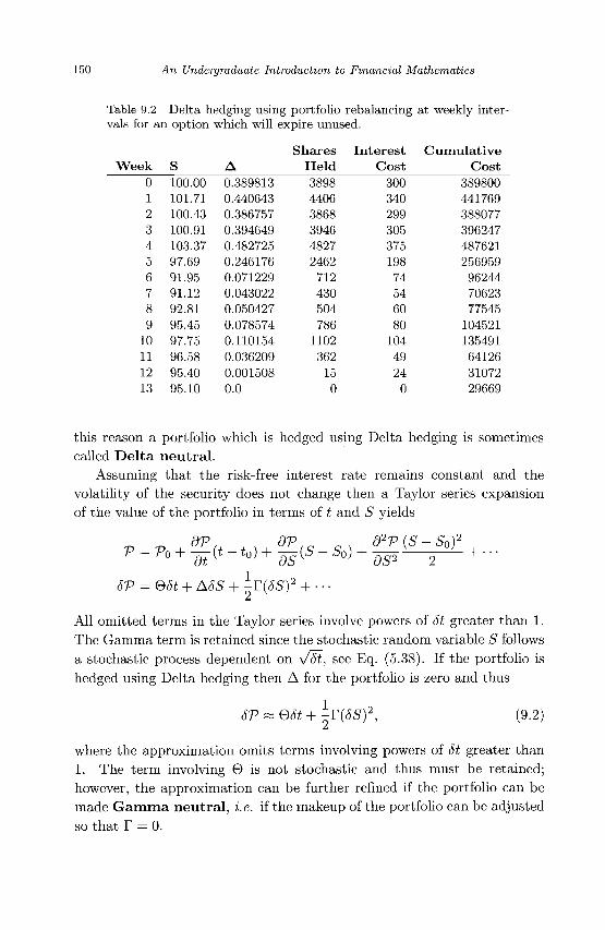
150 An Undergraduate Introduction to Financial Mathematics
Table 9.2 Delta hedging using portfolio rebalancing at weekly intervals for an option which will expire unused.
ek 0 1 2 3 4 5 6 7 8 9 10 11 12 13
S 100.00
101.71
100.43
100.91
103.37
97.69
91.95
91.12
92.81
95.45
97.75
96.58
95.40
95.10
A 0.389813
0.440643
0.386757
0.394649
0.482725
0.246176
0.071229
0.043022
0.050427
0.078574
0.110154
0.036209
0.001508
0.0
Shares
Held
3898
4406
3868
3946
4827
2462
712 430 504 786 1102
362 15 0
Interest
Cost
300 340 299 305 375 198 74 54 60 80 104 49 24 0
Cumulative
Cost
389800
441769
388077
396247
487621
256959
96244
70623
77545
104521
135491
64126
31072
29669
this reason a portfolio which is hedged using Delta hedging is sometimes
called D e l t a neutral . Assuming tha t the risk-free interest ra te remains constant and the
volatility of the security does not change then a Taylor series expansion
of the value of the portfolio in terms of t and S yields
^ ^ dV, , dVln 0 N d2V (S - S0)2
v = r0 + ^(t-to) + -(s-s0) + ^—J-L + -
sv = est + ASS + ^r(ss)2 + • • • All omitted terms in the Taylor series involve powers of St greater than 1.
The Gamma term is retained since the stochastic random variable S follows
a stochastic process dependent on vSt, see Eq. (5.38). If the portfolio is
hedged using Delta hedging then A for the portfolio is zero and thus
sv^est + ^r(ss)2, (9.2)
where the approximation omits terms involving powers of St greater than
1. The term involving 9 is not stochastic and thus must be retained;
however, the approximation can be further refined if the portfolio can be
made G a m m a neutral , i.e. if the makeup of the portfolio can be adjusted
so tha t r = 0.
Hedging 151
9.4 Gamma Neutral Portfolios
Gamma for a portfolio is the second partial derivative of the portfolio with respect to S. The portfolio cannot be made gamma neutral using a linear combination of just an option and its underlying security, since the second derivative of S with respect to itself is zero. As explained in the previous section, the portfolio can be made Delta neutral with the appropriate combination of the option and the underlying security. The portfolio can be made Gamma neutral by manipulating a component of the portfolio which depends non-linearly on S. One such component is the option. However, as mentioned earlier, the portfolio cannot contain only the option and its underlying security. One way to achieve the goal of a Gamma neutral portfolio is to include in the portfolio two (or perhaps more) different types of option dependent on the same underlying security. For example suppose the portfolio contains options with two different strike times written on the same stock. An investment firm may sell a number of European call options with the expiry date three months hence and buy some other number of the European call options on the same stock with an expiry date arriving in six months. Let the number of the early option sold be we and the number of the later option be wi. The Gamma of the portfolio would be
T-p = weTe - wiTi,
where Te and Ti denote the Gammas of the earlier and later options respectively. The relative weights of the earlier and later options can be chosen so that T-p = 0. Once the portfolio is made Gamma neutral, the underlying security can be added to the portfolio in such a way as to make the portfolio Delta neutral. The reader should keep in mind that the underlying security will have a V = 0 and thus Gamma neutrality for the portfolio will be maintained while Delta neutrality is achieved. Thus Eq. (9.2) for a Gamma neutral portfolio reduces to
SP « est. (9.3)
Example 9.2 Suppose a stock's current value is $100 while its volatility is a = 0.22 and the risk-free interest rate is 2.5% per year. An investment firm sells a European call option on this stock with a strike time of three months and a strike price of $102. The firm buys European call options on the same stock with the same strike price but with a strike time of six months. According to Eq. (8.10) the Gamma of the three-month option is T3 = 0.03618, while that of the six-month options is T6 = 0.02563. The
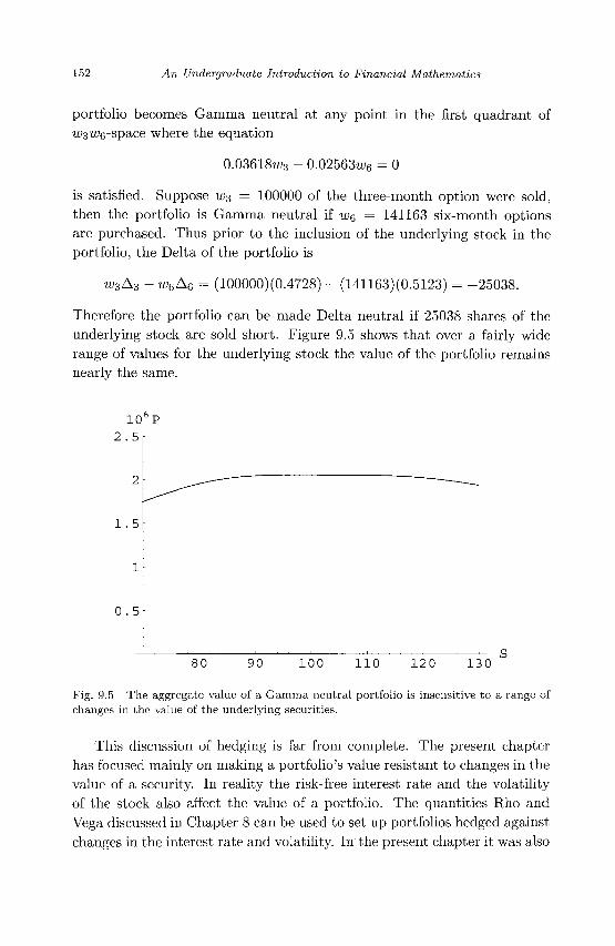
152 An Undergraduate Introduction to Financial Mathematics
portfolio becomes Gamma neutral at any point in the first quadrant of u>3u;6-space where the equation
0.03618w3 - 0.02563w6 = 0
is satisfied. Suppose W3 = 100000 of the three-month option were sold, then the portfolio is Gamma neutral if w6 = 141163 six-month options are purchased. Thus prior to the inclusion of the underlying stock in the portfolio, the Delta of the portfolio is
W3A3 - w6A6 = (100000)(0.4728) - (141163)(0.5123) = -25038.
Therefore the portfolio can be made Delta neutral if 25038 shares of the underlying stock are sold short. Figure 9.5 shows that over a fairly wide range of values for the underlying stock the value of the portfolio remains nearly the same.
106P 2.5r
1.5-
1-
0.5-
, ^ S 80 90 100 110 120 130
Fig. 9.5 The aggregate value of a Gamma neutral portfolio is insensitive to a range of changes in the value of the underlying securities.
This discussion of hedging is far from complete. The present chapter has focused mainly on making a portfolio's value resistant to changes in the value of a security. In reality the risk-free interest rate and the volatility of the stock also affect the value of a portfolio. The quantities Rho and Vega discussed in Chapter 8 can be used to set up portfolios hedged against changes in the interest rate and volatility. In the present chapter it was also
Hedging 153
assumed that the necessary options and securities could be bought so as to form the desired hedge. In practice this may not always be possible. For example an investment firm may not be able to purchase sufficient quantities of a stock to make their portfolio Delta or Gamma neutral. In this case they may have to substitute a different, but related security or other financial instrument in order to set up the hedge. This strategy will be discussed in the next chapter after the prerequisite statistical concepts are introduced.
9.5 Exercises
(1) A call option closes "in the money" if the market price of the underlying security exceeds the strike price for the call option at the time the option matures. Use Eq. (7.35) to show that A —> 1 as t —> T~ for an "in the money" European call option.
(2) A call option closes "out of the money" if the strike price for the call option exceeds the market price of the underlying security at the time the option matures. Use Eq. (7.35) to show that A —> 0 as t —> T~ for an "out of the money" European call option.
(3) Suppose the price of a stock is $45 per share with volatility a = 0.20 per annum and the risk free interest rate is 4.5% per year. Create a table similar to Table 9.1 for European call options on 5000 shares of the stock with a strike price of $47 per share and a strike time of 15 weeks. Rebalance the portfolio weekly assuming the weekly prices of the stock are as follows.
Week S
Week S
0 45.00
8 47.79
1 44.58
9 48.33
2 46.55
10 48.81
3 47.23
11 51.36
4 47.62
12 52.06
5 47.28
13 51.98
6 49.60
14 54.22
7 50.07
15 54.31
(4) Repeat exercise 3 for the following scenario in which the call option finishes out of the money.
Week S
Week
S
0 45.00
8 41.94
1 44.58
9 42.72
2 45.64
10 44.83
3 44.90
11 44.93
4 43.42
12 44.19
5 42.23
13 41.77
6 41.18
14 39.56
7 41.52
15 40.62
154 An Undergraduate Introduction to Financial Mathematics
(5) Repeat exercise 3 assuming this time that the financial institution has issued a European put option for the stock.
(6) Repeat exercise 4 assuming this time that the financial institution has issued a European put option for the stock.
(7) Set up a Gamma neutral portfolio consisting of European call options on a security whose current value is $85. Suppose the risk-free interest rate is 5.5% and the volatility of the security is 17% per year. The portfolio should contain a short position in four-month options with a strike price of $88 and a long position in six-month options with the same strike price.
(8) For the portfolio described in exercise 7 add a position in the underlying security so that the portfolio is also Delta neutral.
(9) Set up a Gamma neutral portfolio consisting of European call options on a security whose current value is $95. Suppose the risk-free interest rate is 4.5% and the volatility of the security is 23% per year. The portfolio should contain a short position in three-month options with a strike price of $97 and a long position in five-month options with a strike price of $98.
(10) For the portfolio described in exercise 9 add a position in the underlying security so that the portfolio is also Delta neutral.
Chapter 10
Optimizing Portfolios
There are several notions of the idea of optimizing a portfolio of securities, options, bonds, cash, etc. In this chapter we will explore optimality in the sense of maximizing the rate of return, minimizing the variance in the rate of return, and minimizing risk to the investor. We will also introduce the Capital Assets Pricing Model which attempts to relate the rate of return of a specific investment to the rate of return for the entire market of investments. We will see in this chapter that the difference in the expected rates of return for a specific security and the risk-free interest rate is proportional to the difference in the expected rates of return for the market and the risk-free interest rate. In order to explain this proportionality relationship we will introduce two additional statistical measures, covariance and correlation. We will also make use of these concepts in developing additional hedging strategies.
10.1 Covariance and Correlation
The concept of covariance is related to the degree to which two random variables tend to change in the same or opposite direction relative to one another. If X and Y are the random variables then mathematically the covariance, denoted Cov(X,Y), is defined as
Cov (X, Y)=E[(X-E [X])(Y - E [Y])}. (10.1)
155
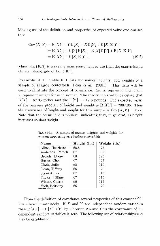
156 An Undergraduate Introduction to Financial Mathematics
Making use of the definition and properties of expected value one can see
tha t
Cov (X, Y)=E [XY - YE [X] - XE [Y] + E [X] E [Y]}
= E [XY] - E [Y] E [X] - E [X] E [Y] + E [X] E [Y]
= E [XY] - E [X] E [Y], (10.2)
where Eq. (10.2) is generally more convenient to use than the expression in
the right-hand side of Eq. (10.1).
E x a m p l e 10 .1 Table 10.1 lists the names, heights, and weights of a
sample of Playboy centerfolds [Dean et al. (2001)]. This da ta will be
used to illustrate the concept of covariance. Let X represent height and
Y represent weight for each woman. The reader can readily calculate tha t
E [X] = 67.05 inches and the E [Y] = 117.6 pounds. The expected value
of the pairwise product of height and weight is E [XY] = 7887.85. Thus
the covariance of height and weight for this sample is Cov(X,Y) = 2.77.
Note tha t the covariance is positive, indicating tha t , in general, as height
increases so does weight.
Table 10.1 A sample of names, heights, and weights for women appearing as Playboy centerfolds.
N a m e Allias, Henriette Anderson, Pamela Broady, Eloise Butler, Cher Clark, Julie Sloan, Tiffany Stewart, Liz Taylor, Tiffany Witter, Cherie York, Brittany
Height (in.) 68.5 67 68 67 65 66 67 67 69 66
Weight (lb.) 125 105 125 123 110 120 116 115 117 120
From the definition of covariance several properties of this concept fol
low almost immediately. If X and Y are independent random variables
then E [XY] = E [X] E [Y] by Theorem 2.5 and thus the covariance of in
dependent random variables is zero. The following set of relationships can
also be established.
Optimizing Portfolios 157
Theorem 10.1 Suppose X, Y', and Z are random variables, then the following statements are true:
(1) C o v ( Z , X ) = V a r ( X ) , (2) Cov (X, Y) = Cov (Y, X), (3) Cov (X + Y,Z) = Cov (X, Z) + Cov (Y, Z).
The proofs of the first two statements are left for the reader as exercises. Justification for statement 3 is given below.
Proof. Let X,Y, and Z be random variables, then
Cov {X + Y, Z) = E [{X + Y)Z] - E [X + Y] E [Z]
= E [XZ] + E [YZ] - E [X] E [Z] - E [Y] E [Z]
= E [XZ] - E [X] E [Z] + E [YZ] - E [Y] E [Z]
= Cov {X, Z) + Cov (Y, Z)
• The third statement of Theorem 10.1 can be generalized as in the fol
lowing corollary.
Corollary 10.1 Suppose {XL, X 2 , . . . , Xn} and {Y1; Y2, . . . , Ym} are sets of random variables where n,m > 1.
( n m \ n m
j = i i = i / i - i j = i
Proof. We begin by demonstrating the result when m = 1. The corollary holds trivially when n = \ and follows from the third statement of Theorem 10.1 when n = 2. Suppose the claim holds when n < k where fcgN. Let {Xi, X 2 , . . . , Xk, Xk+i} be random variables.
C o W f ^ Y i j = C o v f ^ X ^ y i J + Cov(Xfc+1,Y1)
fc = ^ Cov (Xi ,Y1)+ Cov (Xfe+i, Yi)
i = i
fc+i
= ]TCov(Xi,Y1)
158 An Undergraduate Introduction to Financial Mathematics
Therefore by induction we may show that the result is true for any finite, integer value of n (at least when m = 1). Now we can relax the assumption on m. Suppose the claim has been proved for m < k where again k & N. Let {Yi, Y2, . . . , Yfc, Yfc+i} be random variables, then
n fc+1 \ /fc+1 n
Cov(Ex-Ey0 =Cov £y'-'£* k I n \ / n N
= ^ Cov Yj: 5 ] X, + Cov Yfe+1, ^ ^ j=l \ i=l / V i=l /
fc / n \ / n ^
= E Cov Ex*>YJ + Cov E x ^ F^+i k n n
= E E Cov (**- F J ) + E Cov ( x - ^+1) J—12=1 2=1
n k n
= E E Cov (*<> + E Cov ( x - y*+i) i = l ,7 = 1 i = l
n fc+1
= EECov(x-^)
Therefore Eq. (10.3) holds all finite, positive integer values of m, and n. •
Yet another corollary follows from Corollary 10.1. This one generalizes statement 1 of Theorem 10.1.
Corollary 10.2 If {Xi, X2, • • •, Xn} are random variables then
Var ^ Xt = Y,Var (*0 + E E Cov (**> *>) • ( 1 0- 4)
Optimizing Portfolios 159
Proof. Let Y = Y^i=i %i> t n e n according to the first statement of Theorem 10.1,
Var (Y) = Cov (Y, Y)
/ n \ / n n
Var K ^ = Cov E * i , E * . v«=l / \ i= l j —1
n n
= E E Cov (x*' X J ) (by C o r o l l a ry i0-1) n n n
= J2 Cov (<- ) +EE Cov (**> x i ) z=l z=l j ^ z
n n n
= J ] Var {Xi) + E E Cov (**' *i)
Once more the first statement of Theorem 10.1 was used to reintroduce the variance in the last line of the derivation. •
Often a quantity related to covariance is used as a measure of the degree to which large values of a random variable X are associated with large values of another random variable Y. This quantity is known as correlation and is denoted p (X, Y). The correlation of two random variables is defined as
The correlation of two random variables can be interpreted as a measure of the degree to which one of the variables can be written as a linear function of the other. The correlation is more than just a simple re-scaling of the covariance. While the covariance of X and Y may numerically be positive, negative, or zero, the correlation always lies in the interval [—1,1]. Once again we see that independent random variables have a correlation of zero and hence are described as uncorrelated.
Theorem 10.2 Suppose X and Y are random variables such that Y = aX + b where a, b G R with a / 0 . If a > 0 then p (X, Y) = 1, while if a < 0 then p(X,Y) = - 1 .
160 An Undergraduate Introduction to Financial Mathematics
Proof. We start by calculating the covariance of X and Y.
Cov (X, Y) = Cov (X, aX + b)
= E [X{aX + b)} - E [X] E [aX + b]
= E [aX2 + bX)] - E [X] (oE [X] + b)
= aE [X2] + bE [X] - aE [X] E [X] - 6E [X]
= a (E [X2] - E [X]2)
= aVar (X)
The reader should make note of the use of Theorem 2.3. Therefore using the result of exercise 18 from Chapter 2
p(X,Y)~ a V a r W
VVar (X) • a2Var (X) \a\
which is —1 when a < 0 and 1 when a > 0. •
Before we can bound the correlation in the interval [—1,1] we will need to prove the following lemma.
Lemma 10.1 (Schwarz Inequality) If X and Y are random variables then (E [XY])2 < E [X2] E [Y2].
Proof. The cases in which E [X2] = 0, E [X2] = oo, E [Y2] = 0, or E [y2] = oo are left as exercises. Suppose for the purposes of this proof that 0 < E [X2] < oo and 0 < E [Y2] < oo. If a and b are real numbers then the following two inequalities hold:
0 < E [(aX + bY)2] = a2E [X2] + 2abE [XY] + b2E [Y2]
0 < E [(aX - bY)2] = a2E [X2] - 2abE [XY] + b2E [Y2]
If we let a2 = E [Y2] and b2 = E [X2] then the first inequality above yields
0 < E [Y2] E [X2] + 2y/E[Y2]E[X2]E [XY] + E [X2] E [Y2]
- 2 E [X2] E [Y2] < 2y 'E[y 2 ]E[X 2 ]E [XY]
-^E[X2]E[Y2] < E [XY].
By a similar set of steps the second inequality produces
E [XY] < y/E[X2]E[Y2].
Optimizing Portfolios 161
Therefore, since
- v / E [ X 2 ] E [ y 2 ] < E [XY] < y/E [X2] E [Y2]
(E[XY]f < E [ X 2 ] E [ Y 2 ] .
Occasionally (E [XY])2 is written as E [XY]2 or even as E2 [XY]. A careful reading of the expression will avoid any possible confusion. •
Now we are in a position to prove the following theorem.
Theorem 10.3 If X and Y are random variables then — 1 < p(X,Y) < 1.
Proof. Consider the covariance of X and Y.
(Cov (X, Y))2 = (E [{X - E [X])(Y - E [Y])])2
< E [(X - E [X])2] E [(Y - E [Y])2] (by Lemma 10.1)
= Var (X) Var (Y)
Thus |Cov (X, Y) | < y^Var (X) Var (Y), which is equivalent to the inequal
ity,
-VVar (X)Var (Y) < Cov(X,Y) < A/Var (X) Var (Y)
_x < C o v £ £ L < 1 " ^Var (X) Var (Y)
-l<p(X,Y)<l,
which follows from the definition of correlation. D
Example 10.2 Referring to the data in Table 10.1 the correlation between height and weight is calculated as
C 0 V ^ F ) - 2 - 7 ? -0 .3533. ^Var (X) Var (Y) v/(1.46944)(41.8222)
For this data set there does not seem to be an especially strong linear relationship between height and weight. Figure 10.1 illustrates this as well.
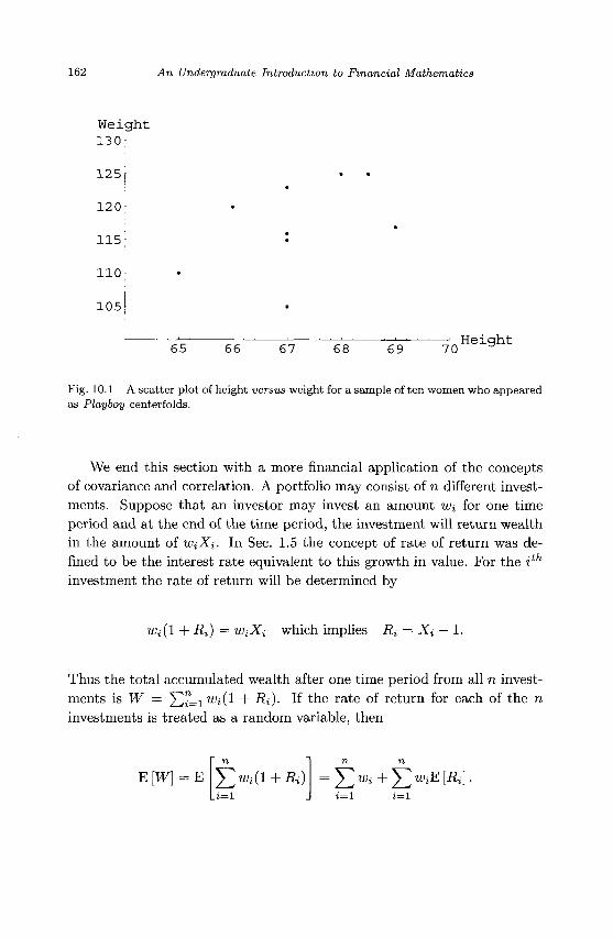
162 An Undergraduate Introduction to Financial Mathematics
Wei 130
125
120
115
110
105
ght
• •
65 66 67 68 69 70 Height
Fig. 10.1 A scatter plot of height versus weight for a sample of ten women who appeared as Playboy centerfolds.
We end this section with a more financial application of the concepts of covariance and correlation. A portfolio may consist of n different investments. Suppose that an investor may invest an amount Wi for one time period and at the end of the time period, the investment will return wealth in the amount of WiXi. In Sec. 1.5 the concept of rate of return was defined to be the interest rate equivalent to this growth in value. For the ith
investment the rate of return will be determined by
Wi(l + Ri) = WiXi which implies Ri = Xi — 1.
Thus the total accumulated wealth after one time period from all n investments is W = X^iLi Wi(l + Ri). If the rate of return for each of the n investments is treated as a random variable, then
E[W]=E J2wi(l + Ri) ^2wi+^2wiE[Ri\.
Optimizing Portfolios 163
The variance in the accumulated wealth is, according to Eq. (10.4),
Var (W) = Var j ^ 1^(1 + ifc) J
= Var ^WiRi J
n n
i=\ i=l j^i n n
= ^2 ^2Var (i?j) + X X WiWjCov (Ri: Rj). 2—1 i=l j^i
Later sections will expand on this idea and develop a method of selecting a portfolio of investments which minimizes the variance in the wealth generated. Minimizing the variance in the rate of return on a portfolio of investments makes the return more "predictable". Remember that the smaller the variance of a random variable, the smaller the spread about the expected value of that variable.
Before concluding this section we will exercise our understanding of co-variance and lognormal random variables to derive a technical result which will be needed in Sec. 10.6.
Lemma 10.2 If X is a lognormal random variable with drift parameter ji and volatility a2 and K > 0 is a constant then
Cov (X, (X - K)+) = E [X(X - K)+] - E [X] E [(X - K)+] , (10.6)
where
E [X(X - K)+] = e2^+a2U(w + 2a) - Ke»+CT*/2(j){w + a), (10.7)
with w = (/i — In K)/a.
Proof. Equation 10.6 follows from the definition of covariance. The technical portion of the lemma is the derivation of Eq. 10.7.
E 1 r00 1
\X(X - K)+] = - L - / x(x - i n + i e - d " * - ^ 2 / 2 " 2 dx 1 J V2^a Jo ' x
= -yL- / (X - # ) e - 0 n * - M ) 2 / 2 ^ ^ V27TCT JK
1 Z"00
= - = / (e"+" - K^^e-*2'2 , V27T J(\nK-n)/a
164 An Undergraduate Introduction to Financial Mathematics
The last equation is derived by making the substitution az = \nx — fi. Therefore
e2(fj.+a2) roo •2(H+o-) poo E [X(X - K)+] = / e ~ ( z - 2 - ) 2 / 2 dz
V27T J(lnK~n)/a
<*-')'/* dz
l(lnK~n)/a
a/J,+a2/2 roo
The proof is complete if we let w = (fi — In K)/a. •
10.2 Optimal Portfolios
In the previous chapter on hedging, all of the discussion and examples assumed that a hedged position with respect to a particular option could be set up by taking a position in the stock or security underlying the option. However, it may not always be possible to purchase (or sell) sufficient shares of the underlying security (or the option itself) to create the hedged position. In these cases the manager of a portfolio may have to find a surrogate for the security. Upon reflection, a particular financial instrument will be a better or worse surrogate for a security depending on how the values of the security and the other instrument change. If the changes in the two values are highly correlated then the portfolio manager will have more confidence in using the surrogate.
Suppose an investment firm sells a European call option for stock A and wishes to create a Delta-neutral portfolio. If insufficient shares of stock A can be purchased to create the hedge then the firm can investigate hedging their short position in the option for stock A with a long position in n shares of stock B. If the hedge could be created with stock A in place of stock B then the Delta-neutral hedge is achieved when n = A as we saw in Sec. 9.2. The issue confronting the investment firm now is, what should n be when the hedge must be created with stock B? An optimal portfolio is one for which the variance in the value of the portfolio in minimized. The value of the portfolio consisting of a short position on a call option for
Optimizing Portfolios 165
stock A and a long position of n shares of stock B will be denoted
V = CA - nB.
The variance in the value of the portfolio is
Var(V) = E [(CA - nB)2] -E[CA- nB}2
= Var (CA) + «2Var (B) - 2nCov (CA, B)
= n2Var (B) - 2nCov (CA, B) + Var (CA) •
Thus it is seen that the variance in the value of the portfolio is a quadratic function of the hedging parameter n. Thus the minimum variance is achieved when
Cov (CA,B) Var (OQ
" " Var(B) = p ( C A ' B ) V ^ r W
Thus if the correlation between the values of the option on stock A and stock B were unity then the hedging parameter would be the ratio of the standard deviations in the value of the option on stock A and the value of stock B. A small correlation between CA and B would indicate that stock B is a poor surrogate for stock A.
The idea of selecting a portfolio by minimizing the variance of its value will be extended in later sections of this chapter. Before returning to minimum variance analysis, we must introduce the concept known as utility and describe its properties.
10.3 Utility Functions
This section will focus on defining and understanding a class of functions which can be used as the basis of rational decision making. Suppose that an investor is faced with the choice of two different investment products. Suppose further that the set of outcomes resulting from investing in either of the products is {Ci, C2 , . . . , C„}. The reader should think of this set of outcomes as the union of the possible outcomes of investing in the first product and the possible outcomes resulting from investing in the second product. The probability of outcome d coming about as the result of investing in the first product will be denoted pi for i = 1, 2 , . . . ,n. If outcome d cannot result from investing in the first product then, of course,
166 An Undergraduate Introduction to Financial Mathematics
Pi = 0. For the second product the values of the probabilities will be denoted qi.
The investor can rank the outcomes in order of desirability, with the most desirable outcome being Ca and the least desirable being Cw. To each of the possible outcomes a utility can be assigned. The utility function u(d) will have a range of [0,1]. To start, u(Ca) = 1 and u{CJ) = 0. The values of u(d) for i ^ a, to will lie in the open interval (0,1). They are assigned as follows. The investor imagines that they have the choice of receiving outcome d with certainty or participating in a random experiment in which they will receive the most desirable outcome Ca with probability u and the least desirable outcome Cw with probability 1 — u. If u = 1 then the investor will surely participate in the random experiment because they will receive Ca with certainty, and they rank this as a more desirable outcome than d- If « = 0 then the investor will definitely not participate in the random experiment since that would result in them receiving the least desirable outcome. They are better off taking the sure outcome d. As u decreases from 1 to 0 there will exist a value of 0 < u < 1 at which the investor will switch from the behavior of participating in the random experiment to taking outcome C, with certainty. This value of u will be the value of u(d). This probability is called the utility of outcome C,. It is assumed that the probability at which the behavior changes is unique. The rational investor once having decided to accept the sure outcome C, will not at a lower probability of receiving Ca decide to once again participate in the random experiment. Thus the utility function is well-defined.
The utility function provides a means by which two outcomes of unequal desirability may be compared. Outcome d is equivalent to receiving Ca with probability u(Ci) or receiving Cw with probability 1 — u(d)- Returning to the original task of deciding between two different investment products, the investor can then understand that investing in the first product is equivalent to receiving Ca with probability
n
^2piu(d), i=l
while the second investment is equivalent to Ca with probability
n
^2qiu(d)-
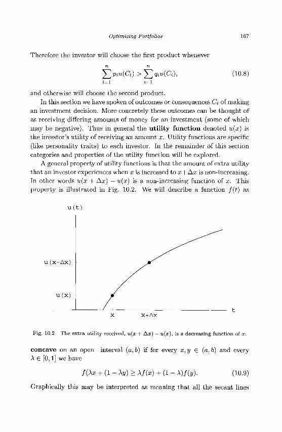
Optimizing Portfolios 167
Therefore the investor will choose the first product whenever
^2piu(d) > y ^ gjUJCj (10.8) 4 = 1
and otherwise will choose the second product. In this section we have spoken of outcomes or consequences Cj of making
an investment decision. More concretely these outcomes can be thought of as receiving differing amounts of money for an investment (some of which may be negative). Thus in general the utility function denoted u{x) is the investor's utility of receiving an amount x. Utility functions are specific (like personality traits) to each investor. In the remainder of this section categories and properties of the utility function will be explored.
A general property of utility functions is that the amount of extra utility that an investor experiences when x is increased to x+Ax is non-increasing. In other words u(x + Ax) — u(x) is a non-increasing function of x. This property is illustrated in Fig. 10.2. We will describe a function f(t) as
u ( t )
u(x+Ax)
u (x )
X+Ax
Fig. 10.2 The extra utility received, u(x + Ax) — u(x), is a decreasing function of x.
concave on an open interval (a, b) if for every x, y G (a, b) and every A € [0,1] we have
/(Ax + (1 - Ay) > A/(x) + (1 - X)f(y). (10.9)
Graphically this may be interpreted as meaning that all the secant lines
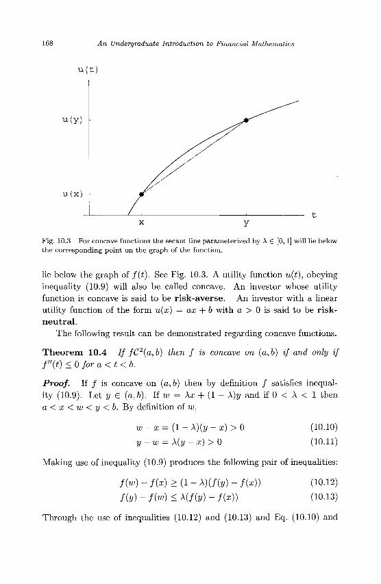
168 An Undergraduate Introduction to Financial Mathematics
U ( t )
u ( y )
u (x )
Fig. 10.3 For concave functions the secant line parameterized by A G [0,1] will lie below the corresponding point on the graph of the function.
lie below the graph of /(£). See Fig. 10.3. A utility function u(t), obeying inequality (10.9) will also be called concave. An investor whose utility function is concave is said to be risk-averse. An investor with a linear utility function of the form u[x) = ax + b with a > 0 is said to be risk-neutral.
The following result can be demonstrated regarding concave functions.
Theorem 10.4 / / fC2(a,b) then f is concave on (a,b) if and only if f"(t) < 0 fora<t<b.
Proof. If / is concave on (a, b) then by definition / satisfies inequality (10.9). Let y E (a, b). If w = Xx + (1 - X)y and if 0 < A < 1 then a < x < w < y <b. By definition of w,
w - x = (1 - X)(y - x) > 0
y — w = X(y — x) > 0
(10.10)
(10.11)
Making use of inequality (10.9) produces the following pair of inequalities:
/ H - fix) > (1 - X)(f(y) - f{x))
f(y) - f(w) < X(f(y) - f{x))
(10.12)
(10.13)
Through the use of inequalities (10.12) and (10.13) and Eq. (10.10) and
Optimizing Portfolios 169
(10.11) we obtain
f(y) - / M < A(/(y) - / H ) = /(y) - /(x) y — w ~ y — w y — x
_{l-X){f{y)-f{x))
<
w — x
w — x
By the Mean Value Theorem [Stewart (1999)] there exist a and /? with x<j3<w<a<y such that
/'(„) = Hv) ~ Hw) < J » ~ /(x) = /' ( /3). y — w w — x
Consequently
a — p
and in the limit we see that
z—>y a — p
To prove the converse suppose /"(x) < 0 on (a,b). Then for any x,y such that a < x < y < b, we can for any A £ (0,1) assign w = Xx + (1 — A)j/ and note that x < w < y.
f(y) - / M < / H - fix)
y — w ~ w — x
From the inequality immediately above it is seen that
/ sf(y) - f(w) , , , , , , s (w - x) < f(w) - f(x)
y-w f(x) + (A, + (1 - X)y - x)f(v)-f& + fi-X)v) < f{Xx + ( 1 _ A ) y )
2/ - Ax - (1 - A)y
/(x) + (1 - A)(„ - *)m-f^-$~X)V) * ^ + (! - A ^ A/(x) + (1 - A)(/(y) - /(Ax + (1 - A)y)) < Xf(Xx + (1 - X)y)
Xf(x) + (1 - A)/(y) < /(Ax + (1 - A)y)
which implies that / is concave on (a, b). •
170 An Undergraduate Introduction to Financial Mathematics
In the next section we will make use of the following result known as Jensen's Inequality.
Theorem 10.5 (Jensen's Inequality (Discrete Version)) Let f be a concave function on the interval (a, b), suppose xt G (a, b) fori = 1,2,... ,n, and suppose Aj S [0,1] for i — 1,2,.. . , n with J27=i » ~ 1> then
n / n \
^ A J t x O ^ / $ > ^ (10.14) i=l \i=l )
Proof. Let ^ = Yl7=i ^iXi anc^ n o t e that s m c e ^i € [0,1] for i = 1, 2 , . . . , n and 5Z"=i -^ = 1> then a < [i < b. The equation of the line tangent to the graph of / at the point (/tx, /(/u)) is y = f'(n)(x — fi) + / ( / / ) . Since / is concave on (a, b) then
/ ( * 0 < f'{n){xi - A*) + /(A*) for i = 1, 2 , . . . n.
Therefore
£ A i / ^ ) < £ (A, [f'(n){xi - M) + /(A*)]) 2 = 1
n n i= l
i= l i= l
i= l
= / ' ( A l ) ( A t - M ^ A i ) + / ( M )
= / ( A 0
V . t = l D
Jensen's inequality may be interpreted as saying that for a concave function, the mean of the values of the function applied to a set of values of a random variable is no greater than the function applied to the mean of the values of the random variable. If u is a concave utility function, then E [upQ] < u(E [X]). Thus a risk-averse investor prefers the certain return of C = E [X] to receiving a random return with this expected value.
Example 10.3 Suppose f(x) = tanhx and let
{A1,A2,A3,A4,A5} = {0.30,0.07,0.23,0.20,0.20}.
Optimizing Portfolios 171
The reader can verify that f(x) is concave on (0, oo). If Xi = i2 for i = 1,2,... ,5 then
J2 W(Xi) = 0.928431 < 1 = / j J2 >*xi)
There is also a continuous version of Jensen's Inequality.
Theorem 10.6 (Jensen's Inequality (Continuous Version)) Let 4>{t) be an integrable function on [0,1] and let f be a concave function, then
fW))dt<f(J <P{t)dt\- (10.15)
Proof. For the sake of compactness of notation let a — J0 <f>{t) dt, and let y = f'(a)(x — a) + f(a), the equation of the tangent line passing through the point with coordinates (a, f{a)). Since / is concave then
fWt))<f'(a)m)-a) + f(a),
which implies that
f im))dt< j f'(a)(<f>(t)-a) + f(a) o Jo
dt
/ ' ( a ) j <j)(t)dt~ [ f'(a)adt+ f f(a)dt Jo Jo Jo
/ ' ( a ) a - / ' ( a ) a + /(a)
f(f mdt a
10.4 Expected Utility
As the name suggests, expected utility is the expected value of a utility function. Returning to the previous discussion of choosing between two possible investment instruments, we see that the investment with the greater expected utility is preferable. The inequality in (10.8) indicated that if the first investment choice results in outcomes {C\, Cg, • • •, C„} with respective probabilities pi for i = 1 2 , . . . n and the second investment choice
172 An Undergraduate Introduction to Financial Mathematics
produces the same outcomes but with probabilities {ft, ft>, • • •, qn} then a rational investor would select the first investment whenever
n n
i = l i = l
Suppose the random variable X is thought of as the set of outcomes with probabilities {Pi,P2, • • • ,Pn} while the random variable Y represents the outcomes with probabilities {ft, 52, • • • , fti}- Then the first investment is preferable whenever
E[u(X)]>E[u(Y)}.
Example 10.4 An investor must choose between the following two "investments" :
A: Flip a fair coin, if the coin lands heads up the investor receives $10, otherwise they receive nothing.
B : Receive an amount $M with certainty.
The investor is risk-averse with a utility function u(x) = x — x2/25. The rational investor will select the investment with the greater expected utility. The expected utility for investment A is
1 1 1 / 102
The expected utility for B is u(M) = M - M 2 /25 . Thus the investor will choose the coin flip whenever
M 2
3 > M - - 2 T M 2 - 25M + 75 > 0
2 5 - 5 ^ 1 3 w — > M. 2
Thus investment A is preferable to B whenever M < $3.49.
If M > $3.49 in the previous example, then the investor will choose the second investment. This illustrates the concept known as the certainty equivalent which is defined as the value C of a random variable X at which u(C) = E[u{X)\.
Example 10.5 An investor wishes to find the certainty equivalent C for the following investment choice:
Optimizing Portfolios 173
A: Flip a fair coin, if the coin lands heads up the investor receives 0 < X < 10, otherwise they receive 0 < Y < X.
B: Receive an amount C with certainty.
Assuming the investor's utility function is the same as in the previous example, the certainty equivalent and payoffs of investment A must satisfy the equation
l(x X\Y Y2\-C C-
C2 -25C+12(X2 + Y2) = 0
25-y/625-48(X2+Y2) C- - .
It is clear from the expression under the radical that the certainty equivalent is real only when X2 + Y2 < 625/48. The design of investment A specifies that 0 < Y < X < 10. Thus the certainty equivalent can be thought of as a surface plotted in cylindrical polar coordinates over the region where 0 < r < -?4= and 0 < 9 < 7r/4. Figure 10.4 illustrates the certainty equivalent as a function of X and Y.
10.5 Portfolio Selection
In the previous sections we have treated the investor's choice between two different investments as a binary, all-or-nothing decision. In reality an investor may choose to split investment capital between two (or more) investments. In this section we will explore the portfolio selection problem, the task of allocating funds in an optimal fashion among several investment options.
We begin with a simple example. Suppose an investor has a total of x amount of capital to invest. Assuming that the investor may use any proportion of this capital, let a £ [0,1] be the proportional they invest. The investment is structured such that an allocation of ax will earn ax with probability p and lose ax with probability 1 —p. Thus for an investment of ax the random variable representing the investor's financial position after the conclusion of the investment is
Y ( x(l + a) with probability p, \x(l — a), with probability 1 — p.
The allocation proportion a will be optimal when the expected value of the
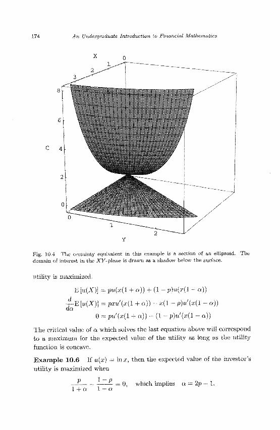
174 An Undergraduate Introduction to Financial Mathematics
Fig. 10.4 The certainty equivalent in this example is a section of an ellipsoid. The domain of interest in the XV-plane is drawn as a shadow below the surface.
utility is maximized.
E [u{X)] - pu(x(l + a)) + (1 - p)u(x(l - a))
-£-E [u(X)\ = pxu'(x(l + a)) - x(l - p)u'{x(l - a)) do,
0 = pu'(x(l + a)) - (1 - p)u'(x(l ~ a))
The critical value of a which solves the last equation above will correspond to a maximum for the expected value of the utility as long as the utility function is concave.
Example 10.6 If u(x) = lax, then the expected value of the investor's utility is maximized when
__" tL — o, which implies a — 2p~ 1. 1 + a 1 — a:
Optimizing Portfolios 175
Thus if p > 1/2 the investor should allocate 100(2p — 1)% of their capital. If 0 < p < 1/2, then E [u(X)] is maximized when a = 0, i.e. when no investment is made. A curve depicting the expected value of the investor's utility as a function of a and p is presented in Fig. 10.5.
E[u(X)]
0.7{
0 . 6 -
0 . 5
0 . 4
0 . 3
0 . 2
0 . 1
0 . 2 0 . 4 0 . 6 0 . 8
Fig. 10.5 The expected value of utility for a risk-averse investor allocating 100(2p— 1)% of their capital.
With this simple example understood, we are now ready to consider a more general situation. Suppose that an amount of capital x may be allocated among n different investments. A proportion xi will be allocated to security i for i = 1, 2 , . . . , n. The vector notation (x\, X2, • • •, xn) will be used to represent the portfolio of investments. The return from investment i will be denoted Wi for i = 1, 2 , . . . , n. The portfolio selection problem is then defined to be that of determining Xi for i = 1, 2 , . . . , n such that
(1) 0 < Xi < 1 for i = 1,2,
(2) £ I U ^ = 1, ,n, and
and which maximizes the investor's total expected utility E [u(VF)], where
n
W = xJ^XiWi.
Throughout this section it will be assumed that n is large and that the Wi's are not too highly correlated. Under these assumptions the Central
176 An Undergraduate Introduction to Financial Mathematics
Limit Theorem of Sec. 3.5 implies that W is a normally distributed random variable.
The allocation of investment funds can be driven by the objective of maximizing the expected value of the investor's utility function. Suppose an investor's utility function is given by u(x) = 1 - e~bx where b > 0. The reader is asked in exercise 12 to show that this utility function is concave and monotonically increasing. Assuming that W i s a normally distributed random variable then — bW is also normally distributed with
E [-bW] = -6E [W] and Var (-bW) = 62Var (W).
Consequently,
E [u{W)\ = E [1 - e'bw] = 1 - E [e-bw] .
Making the assignment Y = e~bw, then Y is a lognormal random variable (see Sec. 3.6). According to Lemma 3.1,
E [Y] = E [e-bW] = e-mw]+b2v^(w)/2
which implies that
Thus the expected utility is maximized when E [W] — &Var (W) /2 is maximized. If two different portfolios, (x\,X2, • • •, xn) and (yi,y2, • • •, Vn), give rise respectively to returns X and Y then the portfolio represented by (xi, X2, • • •, xn) will be preferable if
E [X] > E [Y] and Var (X) < Var (Y).
To extend this discussion and make it more concrete numerically, suppose b = 0.005 and that an investor wishes to choose among an infinite number of different portfolios which can be created by investing in two securities denoted A and B. The investor has $100 to invest and will allocate y dollars to security A and 100 — y dollars to B. The following table summarizes what is known about the rates of return on the hypothetical securities A and B.
Security E [rate of return]
Var (rate of return)
A 0.16 0.20
B 0.18 0.24
Optimizing Portfolios 177
Assume that the correlation between the rates of return is p = —0.35. Once again W will represent the wealth returned.
E [W] = 100 + 0.16y + 0.18(100 - y)
= 118-0.02?/
Var (W) = y2(0.20)2 + (100 - y)2(0.24)2 + 2y(100 - y)(0.20)(0.24)(-0.35)
= 0.04y2 + 0.0576(100 - yf - 0.0336y(100 - y)
Since the optimal portfolio is the one which maximizes E [W] — 6 Var (W) jl then we must maximize
118 - 0.02y - 0.0025(0.04y2 + 0.0576(100 - yf - 0.0336y(100 - y))
= -0.000328j/2 + 0.0172y + 116.56.
This occurs when y sa 26.2195. For this choice of y
E[W] « 117.476
Var(W) « 276.049
E [u{W)\ « 0.442296
In the next section we will generalize and extend these ideas to situations in which investment capital is partitioned n ways.
10.6 Minimum Variance Analysis
Building on the ideas contained in the previous section we consider the case of an investor allocating a portion of their capital between two potential investments. Without loss of generality it is assumed that the investor has an infinitely divisible unit of capital to invest and will invest a fraction a G [0,1] in one security and 1 — a in a second security. The rates of return of the two securities are respectively R\ and i?2- The variances of these rates of return will be denoted cr\ and o\. The covariance in the rates of return is assumed to be c. Thus the variance in the wealth returned from the investments is
Var (W) = o?a\ + (1 - afal + 2ca(l - a) . (10.16)
One measure of an optimal portfolio of investments would be the one with the least variance in the returned wealth. Differentiating Var (W) with
178 An Undergraduate Introduction to Financial Mathematics
respect to a and solving for the critical value of a produces
0 = 2 (aof - (1 - a)a\ + c(l - 2a))
* °2 ~c
a = o\ + o\- 2c
The denominator of a* is the covariance of .Ri — R2 and thus is non-negative. In order for the critical value of a to be defined, it is assumed that a\ +<rf > 2c. This condition is also sufficient to guarantee that the variance of the wealth in Eq. (10.16) will have a global minimum. The parameter a* must also fall within the closed interval [0,1]. This occurs whenever
c < min{(Tj,cr2}.
If c < 0 then this condition is always satisfied. According to the Extreme Value Theorem [Stewart (1999)], the minimum variance will occur when a = 0, a = 1, or a — a*.
Var(W)|Q = 0 = a22
Var(W)|Q = 1=<r?
Consider the special case when the rates of return of the two investments are uncorrelated. Under this assumption c = 0 and the critical value of a at which the variance in the returned wealth is minimized reduces to
2 -i-a* = °l = °l
" n2 , _ 2 l i l '
°1 + a2 -^ + -^ °1 °2
There is an appealing simplicity and symmetry to this critical value. This is not due to coincidence, it is in fact a pattern seen in the more general case of allocating a unit of investment among n different potential investments.
Theorem 10.7 Suppose that 0 < on < 1 will be invested in security i for i = 1,2,..., n subject to the constraint that ct\ + a.?, + • • • + an = 1. Suppose the rate of return of security i is a random variable Ri and that all the rates of return are mutually uncorrelated. The optimal, minimum variance portfolio described by the allocation vector {ai,ct2, • • • , a„ ) , is the
Optimizing Portfolios 179
one for which
— for i = 1,2,.. . , n,
where of = Var (Ri).
Proof. Since the rates are return are uncorrelated then the variance in the returned wealth W is
Var(W0 = 5>?a? , i=l
and is subject to the constraint that 1 = Y^i=i ai- Minimizing the variance subject to the constraint is accomplished by use of Lagrange Multipliers [Stewart (1999)]. This technique states that Var (W) will be optimized at one of the solutions (c*i, a.2, • • ., an, A) of the set of simultaneous equations:
n
The symbol V denotes the gradient operator. These equations are equivalent to respectively:
2aiaf = A for i = 1, 2 , . . . , n, and
n
i = l
Solving for ai in the first equation and substituting into the second equation determines that
9 A En j _
3 = 1 a?
Substituting this expression for A into the first equation yields
l —5"
.n*7' i for i = l , 2 , . . . , n . ^3 = 1 a?
The reader can confirm that for each i, ai € [0,1]. •
180 An Undergraduate Introduction to Financial Mathematics
The previous discussion can be generalized yet again to the situation in which the portfolio of securities is financed with borrowed capital. Let w = (wi, u>2, • • •, wn) represent the portfolio of investments. As before, Ri will represent the return on investing Wi in the ith security. For simplicity's sake we will assume this is a one-period model in which investments are purchased by borrowing money which must be paid back with simple interest of rate r. The return on the portfolio after one time period is
n n n
^(w) = Yl w*(1+Ri)-(l+r)J2Wi = J2 w*(R* -r)- (10-17) 2 = 1 1=1 2 = 1
The expected rate of return on the portfolio and the variance in the rate of return on the portfolio are functions of the vector w and are defined to be respectively,
r(w) = E[#(w)] (10.18)
cr2(w) = Var(i?(w)). (10.19)
In this situation, the borrowed amounts W\, Wi, . . . , wn do not have to sum to unity, or to any other prescribed value.
Lemma 10.3 Assuming the rates of return on the securities are uncorrected, the optimal portfolio with an expected return of unity which minimizes the variance of the portfolio is
I r\—r r^ — r rn—r \ T 2
w * = "-j w, "-j w,..., "-f w) (10.20) <7 = 1 <T? 2->j = j = i ^? 2^j=i m 2->j=i
where ri = E [Ri] and of = Var (Ri) for i = 1, 2 , . . . , n.
The proof of this lemma is similar to the proof of Theorem 10.7 and is left as an exercise.
The existence of the optimal portfolio w* provided by Lemma 10.3 will be used in the following result known as the Portfolio Separation Theorem.
Theorem 10.8 (Portfolio Separation Theorem) Ifb is any positive scalar, the variance of all portfolios with expected rate of return equal to b is minimized by portfolio few* where w* is described in Eq. (10.20).
Optimizing Portfolios 181
Proof. Suppose x is a portfolio for which r(x) = b, then
- r (x ) = r I - x I (by exercise 15)
= 1.
Thus we see that £x is a portfolio with unit expected rate of return. For the portfolio w*,
o-2 (6w*) = & V ( w
>2<
<r2(x) (by exercise 15)
< f r V ( i x ) (by Lemma 10.3)
D
As a consequence of the Portfolio Separation Theorem all expected rates of return on portfolios can be normalized to unity when determining the optimal portfolio.
As a special case of the preceding discussion the investor may wish to divide their portfolio between a risk-free investment such as a savings account and a "risky" investment such as a security. The risk-free interest rate will be symbolized by rf. By assumption the rate of return on the risk-free investment is guaranteed, i.e. has a variance of zero. If the rate of return of the security is Rs and x £ [0,1] is invested in the security while 1 — x is placed in the risk-free investment, the rate of return on the portfolio is
R = (1 — x)rf + xRs,
which implies the expected rate of return for this portfolio is
E [R] = (1 - x)E [rf] + xE {Rs}
= (1 — x)rj + xrs
r = rf + (rs -rf)x (10.21)
To achieve a more compact notation we have set r = E [R] and rs = E [Rs]-Since the risk-free return is a constant, its expected value is this same constant value. The expected rate of return on the portfolio is a linear function of x. The line has its r-intercept at 77 and slope rs — rf. Thus if the expected rate of return of the security exceeds the risk-free rate of return, the slope of the line is positive and the expected rate of return of
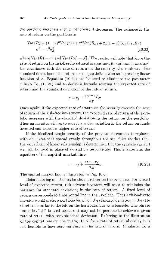
182 An Undergraduate Introduction to Financial Mathematics
the portfolio increases with x, otherwise it decreases. The variance in the rate of return on the portfolio is
Var (R) = (1 - cc)2Var (77) + x2Var (Rs) + 2z(l - x)Cov (77, Rs)
a2 = x2a2s (10.22)
where Var (R) = a2 and Var (-Rs) = a%. The reader will note that since the rate of return on the risk-free investment is constant, its variance is zero and the covariance with the rate of return on the security also vanishes. The standard deviation of the return on the portfolio is also an increasing linear function of x. Equation (10.22) can be used to eliminate the parameter x from Eq. (10.21) and to derive a formula relating the expected rate of return and the standard deviation of the rate of return.
r = rt -\ -a
Once again, if the expected rate of return on the security exceeds the rate of return of the risk-free investment, the expected rate of return of the portfolio increases with the standard deviation in the return on the portfolio. Thus an investor willing to accept a wider variation in the return on funds invested can expect a higher rate of return.
If the idealized single security of the previous discussion is replaced with an investment spread evenly throughout the securities market then the same form of linear relationship is determined, but the symbols TM and UM will be used in place of rs and as respectively. This is known as the equation of the capital market line.
r = rf + rJ£^lLa (10.23)
The capital market line is illustrated in Fig. 10.6. Before moving on, the reader should reflect on the or-plane. For a fixed
level of expected return, risk-adverse investors will want to minimize the variance (or standard deviation) in the rate of return. A fixed level of return corresponds to a horizontal line in the or-plane. Thus a risk-adverse investor would prefer a portfolio for which the standard deviation in the rate of return is as far to the left on the horizontal line as is feasible. The phrase "as is feasible" is used because it may not be possible to achieve a given rate of return with zero standard deviation. Referring to the illustration of the capital market line in Fig. 10.6, for a rate of return above 77 it is not feasible to have zero variance in the rate of return. Similarly, for a
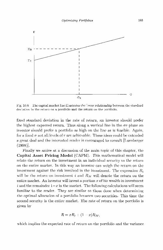
Optimizing Portfolios 183
Fig. 10.6 The capital market line illustrates the linear relationship between the standard deviation in the return on a portfolio and the return on the portfolio.
fixed standard deviation in the rate of return, an investor should prefer the highest expected return. Thus along a vertical line in the or-plane an investor should prefer a portfolio as high on the line as is feasible. Again, for a fixed a not all levels of r are achievable. These ideas could be extended a great deal and the interested reader is encouraged to consult [Luenberger (1998)].
Finally we arrive at a discussion of the main topic of this chapter, the Capital Asset Pricing Model (CAPM). This mathematical model will relate the return on the investment in an individual security to the return on the entire market. In this way an investor can weigh the return on the investment against the risk involved in the investment. The expression Ri will be the return on investment i and RM will denote the return on the entire market. An investor will invest a portion x of his wealth in investment i and the remainder 1—x in the market. The following calculations will seem familiar to the reader. They are similar to those done when determining the optimal allocation of a portfolio between two securities. This time the second security is the entire market. The rate of return on the portfolio is given by
R = xRi + (l- x)R_ M,
which implies the expected rate of return on the portfolio and the variance
184 An Undergraduate Introduction to Financial Mathematics
in the expected rate of return are respectively,
E [R] = xE [Ri] + (1 - x)E [RM]
Var (R) = ir2Var (Ri) + (1 - a;)2Var (RM) + 2x(\ - a;)Cov (Ru RM).
Without further information we cannot assume that the rate of return for investment i is uncorrelated from the rate of return for the market. To simplify the notation we will make the following assignments: r = E[R], n = E[Ri], rM = E[RM], o2 = Var(i?), of = Var(Ri), and o2
M = Var(i?M)- Furthermore we will replace Cov-(R^RM) by its slightly more compact equivalent Pi^u^i^M-1 Thus the equations above become
r = xri + (1 - x)rM (10.24)
o-2 = x2a2 + (1 - x)2a2
M + 2x(l - x)piM<7i<?M- (10.25)
Equations (10.24) and (10.25) can be thought of as the parametric form of a curve in the or-plane. When x = 0, corresponding to the situation in which the entire portfolio is invested in the market, the parametric curve intersects the capital market line. In fact the parametric curve must be tangent to the capital market line at x = 0. If the intersection were transverse rather than tangential, then for some value of x near zero the parametric curve would lie above the capital market line and hence represent an infeasible expected return. Thus we can obtain a relationship between r^, rjvf, and rj. Using Eq. (10.23) to obtain the slope of the capital market line we have
TM -rf _ dr
(JM da dr I dx la:—0 da I dx \x=0
n - rM W7-, °M
Solving the last equation for r» -
n-rf =
- rf yields
Pi,Mai t 77). (10.26) CM
The expression Pi,M&il&M is commonly denoted (3i and is referred to as the be t a of security i. Equation (10.26) can be interpreted as stating that the excess rate of return of security i above the risk-free interest rate is
1This is a small abuse of notation since we normally use P{RI,RM) to denote the correlation of Ri and RM • Here there is little chance of confusion.
Optimizing Portfolios 185
proportional to the excess rate of return of the market above the risk-free interest rate. The proportionality constant is /%. For the case in which the rate of return on security i is uncorrelated with the rate of return on the market, the excess expected return will be zero. When the correlation is positive, excess positive expected return for the market implies excess positive expected return for security i. When the correlation is negative, excess positive expected return for the market will imply excess negative return for security i.
Example 10.7 Suppose the risk-free interest rate is 5% per year, the expected rate of return on the market is 9% per year, and the standard deviation in the return on the market is 15% per year. If the covariance in the expected returns on a particular stock and a the market is 10% then
0 = — : = 4 44444. P (0.15)2
Therefore the expected rate of return on the stock will be
r = 0.05 + 4.44444(0.09 - 0.05) = 0.22777,
or expressed as a percentage return, 22.78%.
The variance in the rate of return of a portfolio can be thought of as a measure of the risk in the portfolio. For a given level of variance in the rate of return, the investor will expect the highest expected value of the rate of return. Thus once again we turn to Lagrange Multipliers to solve this constrained optimization problem. The maximum and minimum value of expected rate of return will occur when
^ = ^ (10-27) ax ax
subject to the constraint expressed in Eq. (10.25). The reader will be asked to verify in the exercises that the solution to this set of equations is
A = ± n~™ = (10.28)
°M ~ Pi,M°iaM
° f + CTM ~~ 2-Pi,MaiaM
[ ^iP2i,M ~ !K2 ( JM + K 2 + ^M
- 2p i i M 0 ' i (TM)0 ' 2
- 2pi,M0'iCrM)0'2
' M ^Pi,M(TiCTM (10.29)
186 An Undergraduate Introduction to Financial Mathematics
Under these conditions the maximum expected rate of return is
(n - rM) (pi,M<TiCrM - <4 ) nnon\ r = rM —,—^ (10.30)
ai + °M ~ 2'Pi,M(Ji(JM 2 0* - rM)\M[M ~ l)aiaM + (°f +aM- IPiMOiOM)**
zp 1 _ ai +(Tll ~ ^Pi,MaiaM
In most scenarios the variance in the rate of return for investment i will exceed the variance for the market. Thus we will assume that ai > GM-As two special cases, we will explore the return on the portfolio when the rates of return on the market and investment i are perfectly correlated, i.e. when piiTn = 1. In this case
(n -rM){<JM ±o-) r = rM .
Oi ~ CM
If the rate of return on investment i is anti-correlated with the rate of return on the market, then
(rt -rM)((?M ±0") r = rM • .
Example 10.8 Suppose the expected rate of return for investment i is Ti = 0.07 with standard deviation CTJ = 0.25 and the expected rate of return for the market is ru = 0.05 with standard deviation OM = 0.20. Suppose the rates of return have a correlation of p^M = 0.57. If an investor is willing to hold a portfolio with a standard deviation in its rate of return at a = 0.22 then the maximum rate of return can be found via the method outlined above. According to Eq. (10.30), the maximum rate of return on the portfolio is 0.0650248. This occurs when x = 0.751242 or when slightly more than 75% of investment capital is placed in investment i. The curve depicting r and x as parametric functions of a is shown in Fig. 10.7.
10.7 Mean Variance Analysis
This chapter concludes with a discussion of the stochastic process approach to determining the expected rate of return of a portfolio. If necessary, the reader may wish to review Chapter 5 before proceeding. In this section the portfolio will consist of positions in a security and a European call option on the security. The reader should not be confused by the portfolio. The investor will purchase a units of the security and b units of the call option,
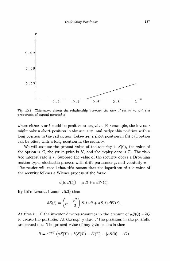
Optimizing Portfolios 187
0 . 0 9
0 . 0 8
0 . 0 7
0 . 2 0 . 4 0.6 0 . 8
Fig. 10.7 This curve shows the relationship between the rate of return r, and the proportion of capital invested x.
where either a or b could be positive or negative. For example, the investor might take a short position in the security and hedge this position with a long position in the call option. Likewise, a short position in the call option can be offset with a long position in the security.
We will assume the present value of the security is S(0), the value of the option is C, the strike price is K, and the expiry date is T. The risk-free interest rate is r. Suppose the value of the security obeys a Brownian motion-type, stochastic process with drift parameter fi and volatility a. The reader will recall that this means that the logarithm of the value of the security follows a Wiener process of the form:
d(lnS(t)) =fidt + (rdW(t).
By Ito's Lemma (Lemma 5.3) then
dS(t) /i + — ) S(t) dt + aS(t) dW(t).
At time t = 0 the investor devotes resources in the amount of aS(0) + bC to create the portfolio. At the expiry date T the positions in the portfolio are zeroed out. The present value of any gain or loss is then
R = e~rT (aS{T) + b(S{T) - K)+) - (aS(0) + bC).
188 An Undergraduate Introduction to Financial Mathematics
Using the linearity property of the expected value, the expected return is
E[R]=E [e~rT (aS(T) + b(S{T) - K)+) - aS(0) - bC]
= e-rTE [aS(T) + b(S(T) - K)+] - a5(0) - bC
= e~rT (aE [S(T)] + bE [(S(T) - K)+]) - aS(0) - bC.
According to Eqs. (5.23) and (5.24) the expected value and variance of In S(T) are respectively
E [In S(T)} = fiT and Var (In S(T)) = a2T.
Thus by Lemma 3.1, E[S(T)] = 5(0)e^+ f f 2 /2)T . Provided that r < n+a2/2 the expression
e-rTE[S(T)} = S{0)e(-r+»+a2/2)T > 5(0).
In order to determine a closed form expression for E [(S(T) — K)+] we will make use of Corollary 3.2. S{T) is a lognormal random variable with parameters In5(0) + fiT (the drift parameter) and CTVT (the volatility parameter). Thus according to Corollary 3.2,
+1 E [(S(T) - K)
= 5(0)^+^)^ (ln5(0)+g-lng + ^
T.,(\n.S{0)+nT-\nK
~ V WT
(HS(0)/K) + fiT
= S(0)e^+a2WT<f> (w + CT\/T) - K<j> (w),
where w = (\n(S(0)/K) + nT)/a\/T. Thus the expected value of the rate of return is
r = E[R] (10.31)
= e-rT (S(0)e^+S^)T (a + bcf>{w + aVf)) - bK<P(w)^j - aS(0) - bC
The level sets of the expected return are lines in the afo-plane.
Optimizing Portfolios 189
The variance in the rate of return can be calculated as
Var (R) = Var (e~rT (aS{T) + b(S{T) - K)+) - aS(0) - bC)
= Var (e~rT (aS{T) + b(S{T) - K)+))
= e-2 r TVar (aS(T) + b(S(T) - K)+)
= e~2rT (a2Var (5(T)) + 62Var ({S(T) - K)+)
+ 2abCov (S{T), (S(T) - K)+)) .
Referring to the second part of Lemma 3.1 we have
Var (S(T)) = S ^ O ^ 2 " * ^ (e^T - l ) .
According to Corollary 3.4,
Var ((S{T) - K)+) = S2(0)e2^+"2)T <l>(w + 2aVT)
- 2KS(0)e^+a^2)T(j)(w + aVf) + K2cj)(w)
w + a
Lemma 10.2 implies that
Cov (S(T), (S(T) - K)+) =KS(0)e^+a2/2)TU{w)-4>(w+aVf)')
- S 2 (0)e 2 ^ + f f 2 ) T U(w+aVT)-^{w+2aVf)^
Putting these last three results together yields, at long last, the complicated, but complete, expression for Var (R).
V&Y(R)=e-2rT(a2S2(0)e^+^T(e°2T-l) (10.32)
+ b2(s2(0)e2^+^T(t>(w+2aVf)-2KS(0)e^+°2WT
(p(w+aVf)
+ K2(t>{w)-(^S(0)e(-fl+a2/2)T(j)(w+(jVT)-K(t){w)y^
+ 2ab(KS(Q)e^+a2 WT (4>(w)-(t>{w+(jy/f))
- S2{0)e2^+a2)T((l){w+aVf)-4>(w+2(TVf)^S)
The level sets of Var (R) are parabolas in the afo-plane.
Example 10.9 Suppose a share of a security has a current price of $100 while the drift parameter and volatility of the price of the security are respectively 0.08 and 0.21 per annum. The risk free interest rate is 3.5%
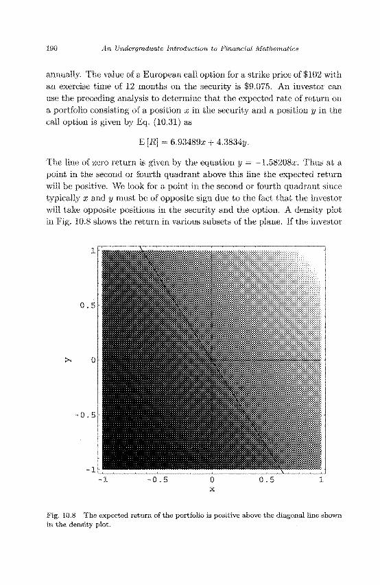
190 An Undergraduate Introduction to Financial Mathematics
annually. The value of a European call option for a strike price of $102 with an exercise time of 12 months on the security is $9,075. An investor can use the preceding analysis to determine that the expected rate of return on a portfolio consisting of a position x in the security and a position y in the call option is given by Eq. (10.31) as
E [R] - 6.93489a) + 4.383%.
The line of zero return is given by the equation y — -1.58208a:. Thus at a point in the second or fourth quadrant above this line the expected return will be positive. We look for a point in the second or fourth quadrant since typically x and y must be of opposite sign due to the fact that the investor will take opposite positions in the security and the option. A density plot in Fig. 10.8 shows the return in various subsets of the plane. If the investor
Fig. 10.8 The expected return of the portfolio is positive above the diagonal line shown in the density plot.
Optimizing Portfolios 191
decides that a return of E [R] = 2 is desirable they will then select x and y so that the variance in the return is minimized over all portfolios for which E [R] = 2. This is yet another constrained optimization exercise. According to Eq. (10.32) the variance in the return is
Var (R) = 515.571a;2 + 748.802x1/ + 306.902y2
Rather than use the method of Lagrange multipliers to find the minimum of Var (R) we will take the more elementary approach of solving the equation 2 = 6.93489a; + 4.3834y for y and substituting into the expression for variance. In this case we get the quadratic expression
Var (R) = 63.891 - 101.421a; + 99.0737a;2
which is minimized when x = 0.511844. Under these conditions y = —0.353511 and the minimum variance is Var (R) = 37.9349.
10.8 Exercises
(1) Using the definition of covariance and variance prove the first two statements of Theorem 10.1.
(2) Show that for any two random variables X and Y
Var (X + Y) = Var {X) + Var (Y) + 2Cov {X, Y).
If X and Y are independent random variables, show this formula reduces to the result mentioned in Theorem 2.7.
(3) Fill in the remaining details of the proof of Lemma 10.1 for the cases in which E [X2] = 0, E [X2] = oo, E [Y2] = 0, or E [Y2] = oo
(4) The data shown in the table below was originally published in the New York Times, Section 3, pg. 1, 05/31/1998. It lists the name of a corporate CEO, the CEO's corporation, the CEO's golf handicap, and a rating of the stock of the CEO's corporation. Determine the covariance and correlation between the CEO's golf handicap, and the corporation's stock rating.
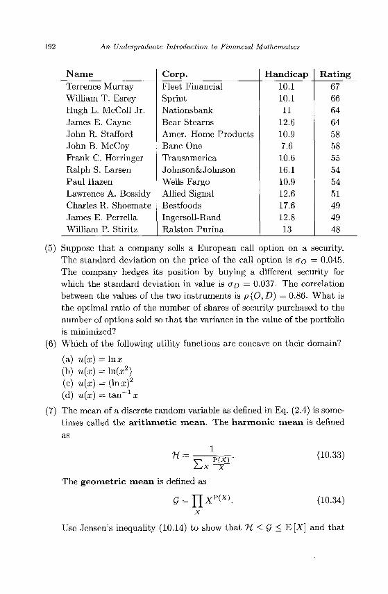
192 An Undergraduate Introduction to Financial Mathematics
Name Terrence Murray William T. Esrey Hugh L. McColl Jr. James E. Cayne John R. Stafford John B. McCoy Frank C. Herringer Ralph S. Larsen Paul Hazen Lawrence A. Bossidy Charles R. Shoemate James E. Perrella William P. Stiritz
Corp. Fleet Financial Sprint Nationsbank Bear Stearns Amer. Home Products Banc One Transamerica Johnsonfe Johnson Wells Fargo Allied Signal Bestfoods Ingersoll-Rand Ralston Purina
Handicap 10.1 10.1 11
12.6 10.9 7.6 10.6 16.1 10.9 12.6 17.6 12.8 13
Rating 67 66 64 64 58 58 55 54 54 51 49 49 48
(5) Suppose that a company sells a European call option on a security. The standard deviation on the price of the call option is ao = 0.045. The company hedges its position by buying a different security for which the standard deviation in value is ar) = 0.037. The correlation between the values of the two instruments is p (O, D) = 0.86. What is the optimal ratio of the number of shares of security purchased to the number of options sold so that the variance in the value of the portfolio is minimized?
(6) Which of the following utility functions are concave on their domain?
(a) u(x) = lnx (b) u(x) = ln(a;2) (c) u(x) = (lnx) (d) u(x) = tan^1 x
(7) The mean of a discrete random variable as defined in Eq. (2.4) is sometimes called the arithmetic mean. The harmonic mean is defined as
H = E x l M 1
The geometric mean is defined as
X
P(X)
(10.33)
(10.34)
Use Jensen's inequality (10.14) to show that H < Q < E [X] and that
Optimizing Portfolios 193
equality holds only when X\ = X2 = • • • = Xn. You may assume that all the random variables are positive.
(8) Verify inequality (10.15) for f(x) = tanha; and <j>(t) = t. (9) Find the certainty equivalent for the choice between (a) nipping a fair
coin and either winning $10 or losing $2, or (b) receiving an amount C with certainty. Assume that your utility function is f(x) = x — x2 /50.
(10) Suppose you must choose between receiving an amount C with certainty or playing a game in a fair die is rolled. If a prime number results you win $15, but if a non-prime number results you lose that amount of money. Assume that your utility function is f(x) = x — x2/2.
(11) Suppose a risk-averse investor with utility function u(x) = In a; will invest a proportion a of their total capital x in an investment which will pay them either 2ax with probability p or nothing with probability 1—p. The amount of capital not invested will earn interest for one time period at the simple rate r. What proportion of their capital should the investor allocate if they wish to achieve the maximum expected utility?
(12) Consider the function u(x) = 1 — e~bx where b > 0.
(a) Show that u(x) is concave. (b) Show that 0 < x\ < X2 implies u(xi) < u(x2)-
(13) Suppose an investor whose utility function is u{x) = 1 — e~x/100 has a total of $1000 to invest in two securities. The expected rate of return for the first investment is 7*1 = 0.08 with a standard deviation in the rate of return of o\ =0.03. The expected rate of return for the second investment is r-i = 0.13 with a standard deviation in the rate of return of CT2 = 0.09. The correlation in the rates of return is p = —0.26. What is the optimal amount of money to place into each investment?
(14) Suppose that an investor will split a unit of wealth between the following securities possessing variances in their rates of return as listed in the table below. Assuming that the rates of return are uncorrelated, determine the proportion of the portfolio which will be allocated to each security so that the variance in the returned wealth is minimized.
Security A B C D E
a2
0.24 0.41 0.27 0.16 0.33
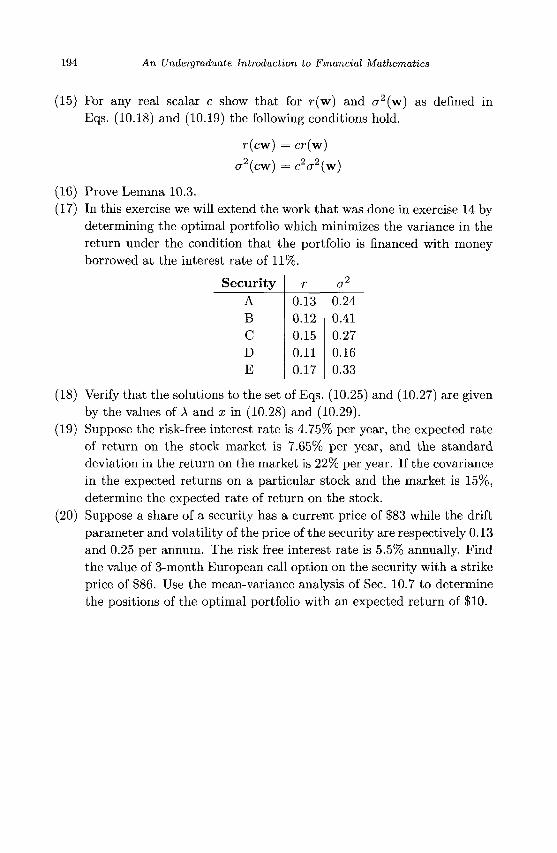
194 An Undergraduate Introduction to Financial Mathematics
(15) For any real scalar c show that for r(w) and er2(w) as defined in Eqs. (10.18) and (10.19) the following conditions hold.
r(cw) = cr(w)
<T2(cw) = C2<T2(w)
(16) Prove Lemma 10.3. (17) In this exercise we will extend the work that was done in exercise 14 by
determining the optimal portfolio which minimizes the variance in the return under the condition that the portfolio is financed with money borrowed at the interest rate of 11%.
Security A B C D E
r 0.13 0.12 0.15 0.11 0.17
a2
0.24 0.41 0.27 0.16 0.33
(18) Verify that the solutions to the set of Eqs. (10.25) and (10.27) are given by the values of A and x in (10.28) and (10.29).
(19) Suppose the risk-free interest rate is 4.75% per year, the expected rate of return on the stock market is 7.65% per year, and the standard deviation in the return on the market is 22% per year. If the covariance in the expected returns on a particular stock and the market is 15%, determine the expected rate of return on the stock.
(20) Suppose a share of a security has a current price of $83 while the drift parameter and volatility of the price of the security are respectively 0.13 and 0.25 per annum. The risk free interest rate is 5.5% annually. Find the value of 3-month European call option on the security with a strike price of $86. Use the mean-variance analysis of Sec. 10.7 to determine the positions of the optimal portfolio with an expected return of $10.
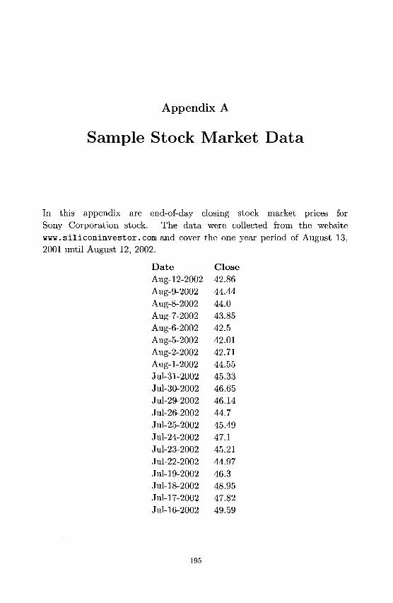
Appendix A
Sample Stock Market Data
In this appendix are end-of-day closing stock market prices for Sony Corporation stock. The data were collected from the website www.siliconinvestor.com and cover the one year period of August 13, 2001 until August 12, 2002.
Date Aug-12-2002 Aug-9-2002 Aug-8-2002 Aug-7-2002 Aug-6-2002 Aug-5-2002 Aug-2-2002 Aug-1-2002 Jul-31-2002 Jul-30-2002 Jul-29-2002 Jul-26-2002 Jul-25-2002 Jul-24-2002 Jul-23-2002 Jul-22-2002 Jul-19-2002 Jul-18-2002 Jul-17-2002 Jul-16-2002
Close 42.86 44.44 44.0 43.85 42.5 42.01 42.71 44.55 45.33 46.65 46.14 44.7 45.49 47.1 45.21 44.97 46.3 48.95 47.82 49.59
195
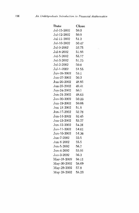
196 An Undergraduate Introduction to Financial Mathematics
Date Jul-15-2002 Jul-12-2002 Jul-11-2002 Jul-10-2002 Jul-9-2002 Jul-8-2002 Jul-5-2002 Jul-3-2002 Jul-2-2002 Jul-1-2002 Jun-28-2002 Jun-27-2002 Jun-26-2002 Jun-25-2002 Jun-24-2002 Jun-21-2002 Jun-20-2002 Jun-19-2002 Jun-18-2002 Jun-17-2002 Jun-14-2002 Jun-13-2002 Jun-12-2002 Jun-11-2002 Jun-10-2002 Jun-7-2002 Jun-6-2002 Jun-5-2002 Jun-4-2002 Jun-3-2002 May-31-2002 May-30-2002 May-29-2002 May-28-2002
Close 50.3 50.9 51.2 50.47 52.75 51.98 53.17 51.75 50.0 51.55 53.1 50.3 48.95 49.41 50.1 48.63 50.23 50.06 51.8 52.78 52.45 53.27 54.31 54.01 54.36 55.5 55.5 56.7 55.91 56.3 58.11 58.69 57.8 58.23
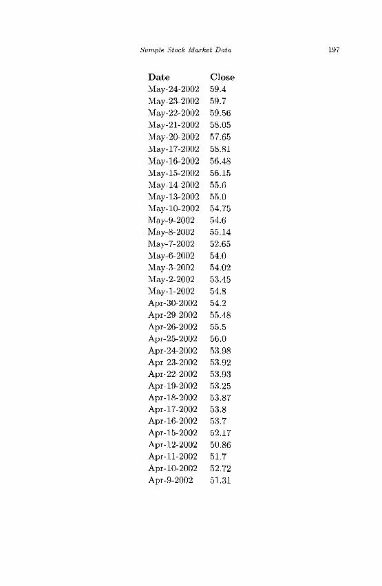
Sample Stock Market Data
Date Close May-24-2002 59.4 May-23-2002 59.7 May-22-2002 59.56 May-21-2002 58.05 May-20-2002 57.65 May-17-2002 58.81 May-16-2002 56.48 May-15-2002 56.15 May-14-2002 55.6 May-13-2002 55.0 May-10-2002 54.75 May-9-2002 54.6 May-8-2002 55.14 May-7-2002 52.65 May-6-2002 54.0 May-3-2002 54.02 May-2-2002 53.45 May-1-2002 54.8 Apr-30-2002 54.2 Apr-29-2002 55.48 Apr-26-2002 55.5 Apr-25-2002 56.0 Apr-24-2002 53.98 Apr-23-2002 53.92 Apr-22-2002 53.93 Apr-19-2002 53.25 Apr-18-2002 53.87 Apr-17-2002 53.8 Apr-16-2002 53.7 Apr-15-2002 52.17 Apr-12-2002 50.86 Apr-11-2002 51.7 Apr-10-2002 52.72 Apr-9-2002 51.31
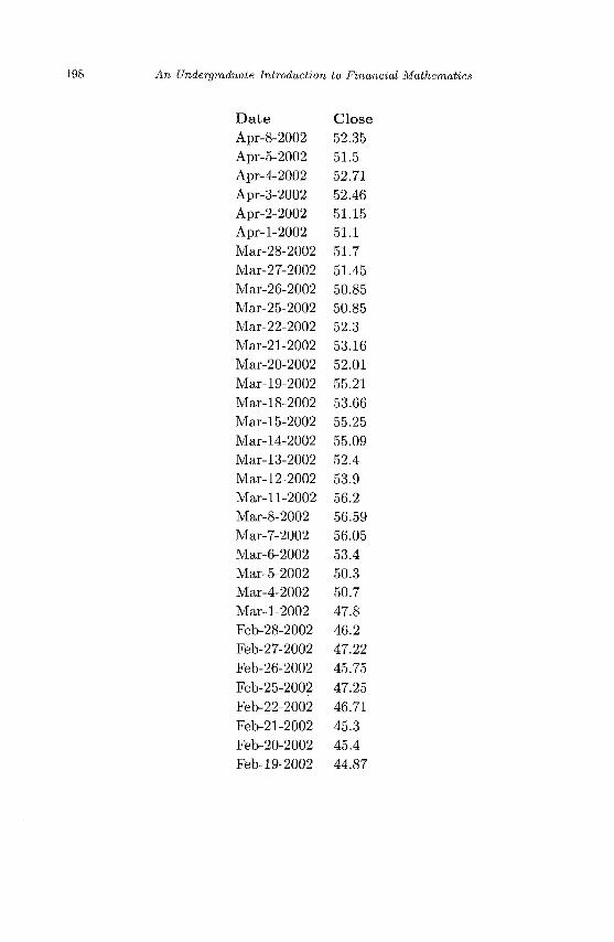
e
I en
m
O
cc
10 csi
CM
co
m
10 lO
lO
N
^f
OO
00 CO
C
O
co in
en 05
m
HO
C1
CO
C<
0^
0)
0|
10
0'
<*
MN
I»
oo
cM
oo
cM
in
'wi
n'i
n'c
MM
co
'co
co
MO
Ot
-P
^C
Mi
—i
CM
CM
^H
rH
^H
rH
OO
CM
CO
C^
lO
CO
lo
mC
NC
OC
OC
OC
OC
OO
OI
^
Wi
ni
nt
nm
in
ww
wm
mm
in
in
wm
mm
mm
mi
om
mL
om
"3
CM
C
M
CM
C
M
CM
o
o
o
o
o
"
O
" ~
CM
CM
CM
CM
CM
CM
CM
CM
CM
CM
CM
CM
CM
CM
o
o
o
o
o
o
o
o
o
o
o
o
1 <
>—
< >
—'
' '
' >
' '
<—
' >
—'
>—
' v
J
i i
i—
i \
—i
v—
/
CM
CM
CM
CM
CM
CM
CM
CM
CM
CM
CM
CM
CM
CM
^"
^^
^^
OO
NO
^M
HO
OI
OO
UJ
^M
OI
H^
^^
CM CM CM CM CM
o o o o o
o
oo m - co
CM
CM CM CM CM CM CM CM
OO N
CO lO ^
iti o
. o
r>. n
. n.
o.
Cc
ia
3c
dc
dc
ga
3g
3a
30
3g
3a
3c
da
3a
3c
dc
dn
3c
c3
a3
a
e
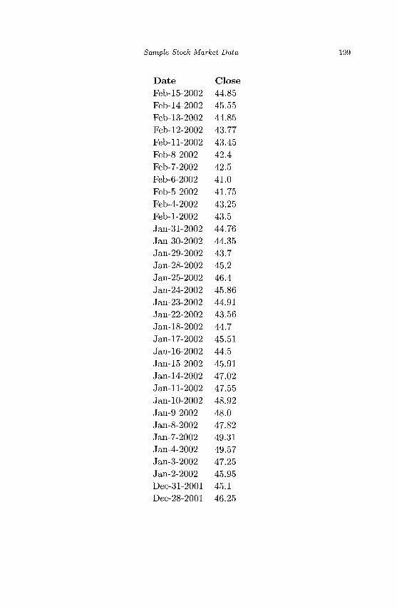
o
o o to
00
to
o
o
h-1
l£>
Ol
to
Cn
u
o
co
h-»
to
o
o
h-'
rf^
Ol
h-1
C-l
95
p to
to
o
o
to
rf^
Cn
CO
Cn
C-l
P P
CO
tO
O o to
rf*.
^1
to
Cn
c^
P 0 f*
to
o
o to
rf^
CO
cn
-a
c^
P p
~J
1
to
o
O to
**
CD
co
H
5-1
P tps
oo
to
o
o
to
rf^
^r
bo
to
c-i
P p
CO
to
o
o to
4^
00
o
C-l
95
P
l—L
cp
to
o
o to
4^
00
CO
to
C-l
p p
1—l
1—l
to
o
o to
*.
J
cn
Cn
t-i
95
P
1—»
i
to
o
o to
£- pj
o to
C-l
95
P
I—1
Cn
to
o
o to
J
en
CO
1—
l
C-l
95
p
1—l
Oi
to
o
o
to
**
^
en
c-<
p p
1—l
-<I
to
o
o to
**
en
en
h^
Cw
p p
H-*
oo
to
o
o to
>£.
**
^
C_l
p p
to
to
to
o
o to
rf^
CO
en
05
C-l
p a to
CO
to
o
o to
J
*
CO
I—1
C-l
p p to
f*"
to
o
o to
>t
en
bo
02
c-
p p to
en
to
o
o to
^
Oi ** o*
p p to
oo
to
o
o to
^
en
to
C-l
p p
to
CD
to
o
o to
rf^
CO
^
C-l
p p
CO
cp
to
o
o to
(J
*"
CO
Cn
CH
p p
CO
F-1
to
o
o to
>£- *"
^
Oi
^
CD
cr
h-1
to
o
o to
*- co
Cn
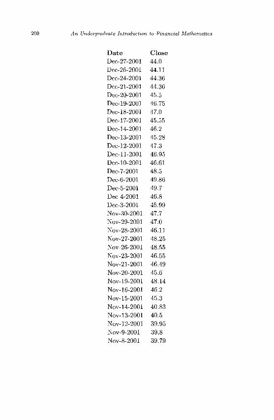
200 An Undergraduate Introduction to Financial Mathematics
Date Close Dec-27-2001 44.0 Dec-26-2001 44.11 Dec-24-2001 44.36 Dec-21-2001 44.36 Dec-20-2001 45.5 Dec-19-2001 46.75 Dec-18-2001 47.0 Dec-17-2001 45.55 Dec-14-2001 46.2 Dec-13-2001 45.28 Dec-12-2001 47.3 Dec-11-2001 46.95 Dec-10-2001 46.61 Dec-7-2001 48.5 Dec-6-2001 49.86 Dec-5-2001 49.7 Dec-4-2001 46.8 Dec-3-2001 45.99 Nov-30-2001 47.7 Nov-29-2001 47.0 Nov-28-2001 46.11 Nov-27-2001 48.25 Nov-26-2001 48.55 Nov-23-2001 46.55 Nov-21-2001 46.49 Nov-20-2001 45.6 Nov-19-2001 48.14 Nov-16-2001 46.2 Nov-15-2001 45.3 Nov-14-2001 40.83 Nov-13-2001 40.5 Nov-12-2001 39.95 Nov-9-2001 39.8 Nov-8-2001 39.79
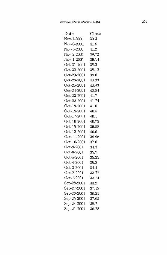
Sample Stock Market Data
Date Close Nov-7-2001 39.3 Nov-6-2001 41.8 Nov-5-2001 41.2 Nov-2-2001 39.72 Nov-1-2001 39.14 Oct-31-2001 38.2 Oct-30-2001 38.12 Oct-29-2001 38.6 Oct-26-2001 40.33 Oct-25-2001 40.43 Oct-24-2001 40.84 Oct-23-2001 41.7 Oct-22-2001 41.74 Oct-19-2001 41.0 Oct-18-2001 40.5 Oct-17-2001 40.1 Oct-16-2001 40.75 Oct-15-2001 39.58 Oct-12-2001 40.01 Oct-11-2001 39.96 Oct-10-2001 37.0 Oct-9-2001 34.31 Oct-8-2001 35.7 Oct-5-2001 35.25 Oct-4-2001 35.3 Oct-3-2001 34.4 Oct-2-2001 33.72 Oct-1-2001 33.74 Sep-28-2001 33.2 Sep-27-2001 37.19 Sep-26-2001 36.25 Sep-25-2001 37.05 Sep-24-2001 38.7 Sep-21-2001 36.75
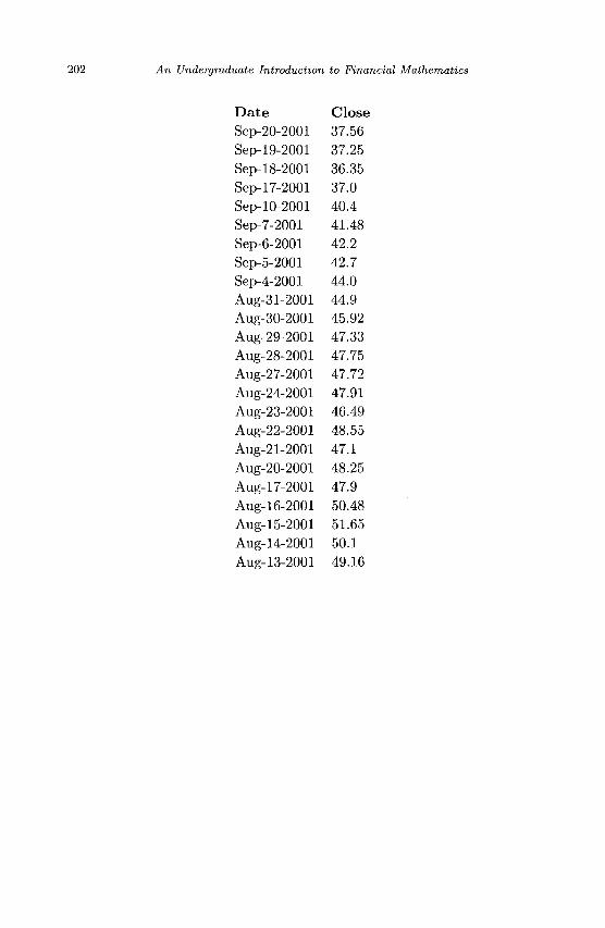
An Undergraduate Introduction to Financial Mathematics
Date Close Sep-20-2001 37.56 Sep-19-2001 37.25 Sep-18-2001 36.35 Sep-17-2001 37.0 Sep-10-2001 40.4 Sep-7-2001 41.48 Sep-6-2001 42.2 Sep-5-2001 42.7 Sep-4-2001 44.0 Aug-31-2001 44.9 Aug-30-2001 45.92 Aug-29-2001 47.33 Aug-28-2001 47.75 Aug-27-2001 47.72 Aug-24-2001 47.91 Aug-23-2001 46.49 Aug-22-2001 48.55 Aug-21-2001 47.1 Aug-20-2001 48.25 Aug-17-2001 47.9 Aug-16-2001 50.48 Aug-15-2001 51.65 Aug-14-2001 50.1 Aug-13-2001 49.16
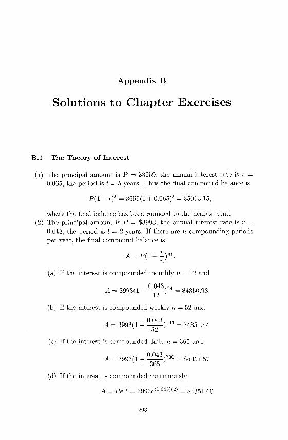
Appendix B
Solutions to Chapter Exercises
B. l The Theory of Interest
(1) The principal amount is P = $3659, the annual interest rate is r = 0.065, the period is t = 5 years. Thus the final compound balance is
P ( l + rf = 3659(1 + 0.065)' = $5013.15,
where the final balance has been rounded to the nearest cent. (2) The principal amount is P = $3993, the annual interest rate is r =
0.043, the period is t = 2 years. If there are n compounding periods per year, the final compound balance is
A = P(l + -)nt. n
(a) If the interest is compounded monthly n = 12 and
A = 3993(1 + 2 ^ 5 ) 2 4 = $4350.93
(b) If the interest is compounded weekly n = 52 and
A = 3993(1 + ^ - ^ ) 1 0 4 = $4351.44 52
(c) If the interest is compounded daily n = 365 and
A = 3993(1 + ^15)730 = $4351.57 365
(d) If the interest is compounded continuously
A = Pert = 3993e(°-043^2) = $4351.60
203

204 An Undergraduate Introduction to Financial Mathematics
(3) The period is t = 1, the interest rate is r = 0.08 compounded n = 4 times per period. The effective simple annual interest rate R is
R = - 1 + (1 + —— )4 = 0.08243216.
(4) Since the competitor pays interest at rate r = 0.0525 compounded daily we will compute his effective simple annual interest rate and then determine the monthly compounded rate which matches it. The effective simple annual interest rate R is
0.0525, 365 R = - 1 + 1 + Y00 = 0.0538985832 365
Thus we wish to solve the following equation for i.
0.058985832 = - 1 + (1 + - ^ ) 1 2
1.058985832 = (1 + - ^ ) 1 2
Vl.058985832 = 1 + —
1.004384268 =1 + ^-
0.004384268 = -^
0.052611220 = i
Thus if you pay an interest rate compounded monthly of at least 5.261122% you will compete favorably.
(5) The continuously compounded interest-bearing account will increase in value more rapidly, thus we wish to solve the following equation.
1 0 0 0 e o ,0475 t _ 1 0 0 0 ( 1 + ^ 0 4 7 5 ) 3 6 5 t = :
365
This equation cannot be solved algebraically for t, so we use Newton's method to approximate the solution, t « 42.6583 years.
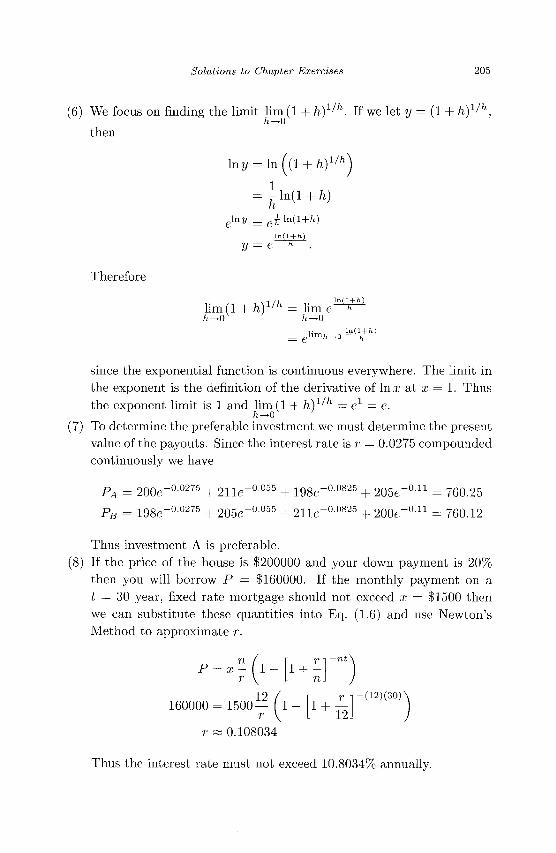
Solutions to Chapter Exercises 205
(6) We focus on finding the limit lim (1 + h)l/h. If we let y = (1 + h)l/h, h—>0
then
lny = l n ( ( l + ft)1/'')
ny _
y =
= i ln(l + ft)
= e*ln(l+h) l n ( l + h)
= e h .
Therefore
ln( l + fe) lim(l + ft)1/,l = l i m e " T / I - > 0 h^O
= e
since the exponential function is continuous everywhere. The limit in the exponent is the definition of the derivative of In x at x = 1. Thus the exponent limit is 1 and lim(l + ft)1''1 = e1 = e.
h—*0
(7) To determine the preferable investment we must determine the present value of the payouts. Since the interest rate is r = 0.0275 compounded continuously we have
PA = 200e-°0 2 7 5 + 211e-°-055 + lOSe"00825 + 2 0 5 e - ° n = 760.25
PB = 198e-°0 2 7 5 + 205e-°0 5 5 + 211 e -° 0 8 2 5 + 2 0 0 e - ° n = 760.12
Thus investment A is preferable. (8) If the price of the house is $200000 and your down payment is 20%
then you will borrow P — $160000. If the monthly payment on a t = 30 year, fixed rate mortgage should not exceed x = $1500 then we can substitute these quantities into Eq. (1.6) and use Newton's Method to approximate r.
' = * ; ( '
160000 = 1500— ( l r \
r w 0.108034
T-[ —nt
i + -n
r n - ( 1 2 ) ( 3 0 )
1 + l2
Thus the interest rate must not exceed 10.8034% annually.
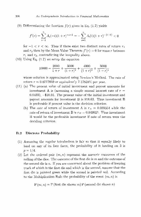
206 An Undergraduate Introduction to Financial Mathematics
(9) Differentiating the function / ( r ) given in Eq. (1.7) yields
n n
/ '(r) = Y, M~i)(l + r)-1'1 =-J2 Mm + r)~iz+1) < 0 i= l i= l
for — 1 < r < co. Thus if there exist two distinct rates of return n and ri then by the Mean Value Theorem / ' ( r ) = 0 for some r between T\ and V2, contradicting the inequality above.
(10) Using Eq. (1.7) we setup the equation
2000 3000 4000 3000
1 + r (1 + r)2 ( 1 + r ) 3 (1 + r)4
whose solution is approximated using Newton's Method. The rate of return r ss 0.0717859 or equivalently 7.17859% per year.
(11) (a) The present value of initial investment and payout amounts for investment A is (assuming a simple annual interest rate of r = 0.0433), —$10.91. The present value of the initial investment and payout amounts for investment B is $18.63. Thus investment B is preferable if present value is the decision criterion.
(b) The rate of return of investment A is TA = 0.039354 while the rate of return of investment B is TB = 0.049921. Thus investment B would be the preferable investment if rate of return were the deciding criterion.
B.2 Discrete Probability
(1) Assuming the regular tetrahedron is fair so that it equally likely to land on any of its four faces, the probability of it landing on 3 is p = 1/4.
(2) Let the ordered pair (m,n) represent the numeric outcomes of the rolling of the dice. The outcome of the first die is m and the outcome of the second die is n. If you are concerned about the problem of keeping track of which is the first die and which is the second, assume that the first die is painted green while the second is painted red. According to the Multiplication Rule the probability of the event (m, n) is
P (m, n) = P (first die shows m) P (second die shows n)
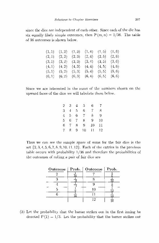
Solutions to Chapter Exercises 207
since the dice are independent of each other. Since each of the die has six equally likely simple outcomes, then P (TO, n) = 1/36. The table of 36 outcomes is shown below.
(1,1) (2,1) (3,1) (4,1) (5,1) (6,1)
(1,2) (2,2) (3,2) (4,2) (5,2) (6,2)
(1,3) (2,3) (3,3) (4,3) (5,3) (6,3)
(1,4) (2,4) (3,4) (4,4) (5,4) (6,4)
(1,5) (2,5) (3,5) (4,5) (5,5) (6,5)
(1,6) (2,6) (3,6) (4,6) (5,6) (6,6)
Since we are interested in the sums of the numbers shown on the upward faces of the dice we will tabulate them below.
4 5 6 7 8 9
5 6 7 8 9 10
6 7 8 9 10 11
7 8 9 10 11 12
Thus we can see the sample space of sums for the fair dice is the set {2, 3, 4, 5, 6, 7, 8, 9,10,11,12}. Each of the entries in the previous table occurs with probability 1/36 and therefore the probabilities of the outcomes of rolling a pair of fair dice are
Outcome 2 3 4 5 6
Prob. l
36 1 18 1 12 1 9 5
36
Outcome 7 8 9 10 11 12
Prob. l 6 5
36 1 9 1
12 1
18 1
36
(3) Let the probability that the batter strikes out in the first inning be denoted P (1) = 1/3. Let the probability that the batter strikes out
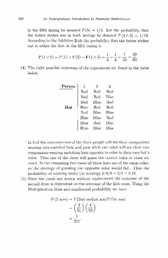
208 An Undergraduate Introduction to Financial Mathematics
in the fifth inning be denoted P (5) = 1/4. Let the probability that the batter strikes out in both innings be denoted P (1 A 5) = 1/10. According to the Addition Rule the probability that the batter strikes out in either the first or the fifth inning is
P ( l V 5 ) = P ( l ) + P ( 5 ) - P ( l A 5 ) = i + i - ^ = | .
(4) The eight possible outcomes of the experiment are listed in the table below.
Person
Ha t
1 Red Red Red Blue Red Blue Blue Blue
2 Red Red Blue Red Blue Blue Red Blue
3 Red Blue Red Red Blue Red Blue Blue
In 6 of the outcomes two of the three people will see their companions wearing mis-matched hats and pass while the third will see their two companions wearing matching hats opposite in color to their own hat's color. Thus one of the three will guess the correct color in these six cases. In the remaining two cases all three hats are of the same color, so the strategy of guessing the opposite color would fail. Thus the probability of winning under the strategy is 6/8 = 3/4 = 0.75.
(5) Since the cards are drawn without replacement the outcome of the second draw is dependent on the outcome of the first draw. Using the Multiplication Rule and conditional probability we have
P (2 aces) = P (2nd acejlst ace) P (1st ace)
= [bl) (,52 J 1
~ 221'
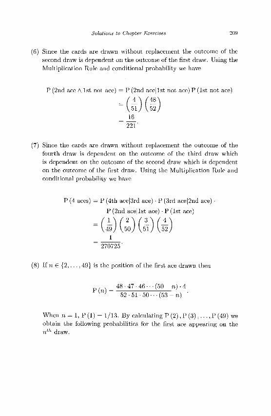
Solutions to Chapter Exercises 209
(6) Since the cards are drawn without replacement the outcome of the second draw is dependent on the outcome of the first draw. Using the Multiplication Rule and conditional probability we have
P (2nd ace A 1st not ace) = P (2nd ace 11st not ace) P (1st not ace)
4 \ /48N
51 J V 52 16
221'
(7) Since the cards are drawn without replacement the outcome of the fourth draw is dependent on the outcome of the third draw which is dependent on the outcome of the second draw which is dependent on the outcome of the first draw. Using the Multiplication Rule and conditional probability we have
P (4 aces) = P (4th ace 13rd ace) • P (3rd ace 12nd ace) •
P (2nd ace11st ace) • P (1st ace)
= (49J (,50 J (,51J \52j _ 1 ~ 270725'
(8) If n £ {2 , . . . , 49} is the position of the first ace drawn then
48 • 47 • 46 • • • (50 - n) • 4 (n)
5 2 - 5 1 - 5 0 - - - ( 5 3 - n )
When n = 1, P (1) = 1/13. By calculating P (2), P ( 3 ) , . . . , P (49) we obtain the following probabilities for the first ace appearing on the nth draw.
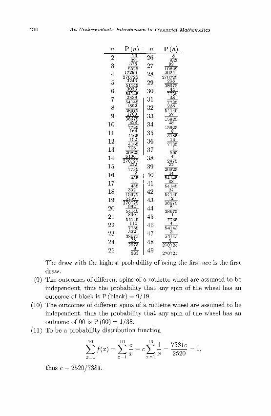
210 An Undergraduate Introduction to Financial Mathematics
P(n) 2 3 4
5 6 7 8 9
10 11
12
13 14 15
16 17 18
19 20 21 22
23 24
25
16 221 376 5525
17296 270725 3243 54145 3036 54145 2838 54145 1892 38675 1763 38675 328 7735 164 4165 152 4165 703 20825 8436 270725
222 7735 12 455 11 455 352 15925 5456 270725 992 54145 899 54145 116 7735 522 38675 36 2975 9
26 27 28 29 30 31 32 33 34 35 36 37 38 39 40 41 42 43 44 45 46 47 48 49
P(n)
833 92
10829 2024 270725 253 38675 44 7735 38 7735 228 54145 57
15925 48 15925 8
3185 16
7735 1
595 4
2975 22
20825 44
54145 33
54145 24
54145 12
38675 8
38675 1
7735 4
54145 2
54145 4
270725 1
270725
The draw with the highest probability of being the first ace is the first draw.
(9) The outcomes of different spins of a roulette wheel are assumed to be independent, thus the probability that any spin of the wheel has an outcome of black is P (black) = 9/19.
(10) The outcomes of different spins of a roulette wheel are assumed to be independent, thus the probability that any spin of the wheel has an outcome of 00 is P (00) = 1/38.
(11) To be a probability distribution function
10 10 10
2 = 1
7381c 2520
= 1,
thus c = 2520/7381.
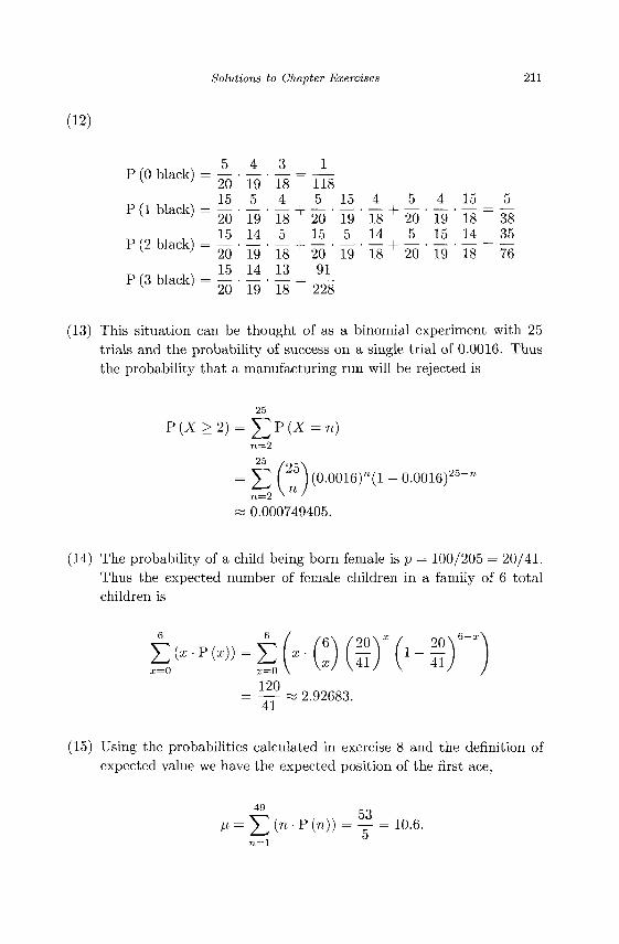
Solutions to Chapter Exercises 211
(12)
5 20 ' 15 20 ' 15 20 ' 15 20 '
4 ' 19 ' 5 19' 14 19 ' 14 ' 19 '
3 1 18 ~ 118 4 5 15 18 + 20 ' 19 ' 5 15 5 18 + 20 ' 19 ' 13 91 18 ~ 228
4 5 ' 18 + 20 14 5 ' 18 + 20
4 19 15 ' 19
15 ' 18 ~ 14 ' 18 ~
5 : 38 35 76
P (0 black)
P (1 black)
P (2 black)
P (3 black)
(13) This situation can be thought of as a binomial experiment with 25 trials and the probability of success on a single trial of 0.0016. Thus the probability that a manufacturing run will be rejected is
25
P {X > 2) = J^ P (X
n = 2
25
= Yl ( ^ ) (°-0016)n(1 - 0.0016)25"71
w 0.000749405.
(14) The probability of a child being born female is p = 100/205 = 20/41. Thus the expected number of female children in a family of 6 total children is
120 = —- « 2.92683.
41
(15) Using the probabilities calculated in exercise 8 and the definition of expected value we have the expected position of the first ace,
49 5 3
H = J2 (n • P (n)) = — = 10.6. n—1
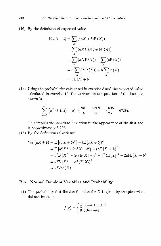
212 An Undergraduate Introduction to Financial Mathematics
(16) By the definition of expected value
E [aX + b] = J2 ((aX + b)F (x)) x
= £ ( a X P ( X ) + 6 P p O ) x
= 5 > X P ( X ) ) + ^ > P ( X ) ) x x
= a£(XPPO)+&X>PO x x
= aE [X] + b
(17) Using the probabilities calculated in exercise 8 and the expected value calculated in exercise 15, the variance in the position of the first ace drawn is
s^ , 2 TW 2 901 2809 1696 „„„„ ^ ( n 2 . P ( n ) ) - M
2 = — - — = — = 6 7 . 8 4 .
n=\
This implies the standard deviation in the appearance of the first ace is approximately 8.2365.
(18) By the definition of variance
Var (aX + b) = E [(aX + b)2] - (E [aX + b})2
= E [a2X2 + 2abX + b2] - (aE [X] + bf
= a2E [X2] + 2abE [X] + b2 -a2 (E [X])2 - 2a6E [X] - b2
= a2E [X2] - a2 (E [X])2
= a2 Var (X)
B.3 Normal Random Variables and Probability
(1) The probability distribution function for X is given by the piecewise defined function
/ ( X ) = ; H - 4 < * < I I 0 otherwise.
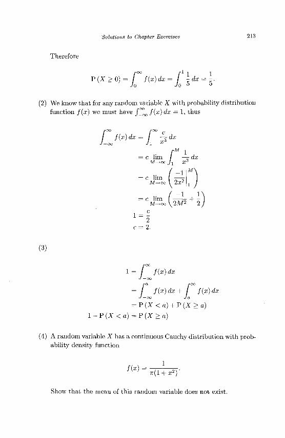
Solutions to Chapter Exercises 213
Therefore
, 0 0 Z"1 1 1 P ( X > 0 ) = / f(x)dx = -dx = -.
Jo Jo 5 5
(2) We know that for any random variable X with probability distribution function f(x) we must have f_ f(x) dx = 1, thus
• dx
(3)
J(x)dx = J^ -$
dx
M>
c lim M-
c lim —-
= CivlToo(2ii + ^
2 c = 2.
/
OO
/(a:) da; -OO
/>0O
f(x)dx+ f{x) (£E
= P (X < a) + P (X > a)
1 - P (X < a) = P (X > a)
(4) A random variable X has a continuous Cauchy distribution with probability density function
/ ( * ) •
1 7r(l + a;2)'
Show that the mean of this random variable does not exist.
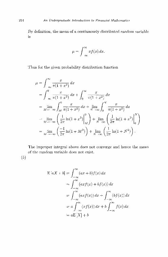
214 An Undergraduate Introduction to Financial Mathematics
By definition, the mean of a continuously distributed random variable is
/
oo
xf(x)dx. -oo
Thus for the given probability distribution function
r(l + a;2) dx
J_ocn(l+x2)dX + J0 TT(1
lim
+ x2) dx
dx + lim M ^ - o o JM 7r(l + X2) N->ooJ0 7r(l + X2)
N
dx
l i m \n(i+xi) M—> —oo \ Z7T M ,
+ lim — ln(l + x2) N\
lim [ — ln(l + M 2 ) ) + lim ( — ln(l + 7V2'
The improper integral above does not converge and hence the mean of the random variable does not exist.
(5)
E [aX + b] — OO
OO
(ax -h b)f(x) dx
(axf(x) + bf(x)) dx
/•OO
(axf (x)) dx-\- / (bf(x))dx
= a / (xf(x)) dx + b J f(x) dx J—OO
= aE [X] + 6
Solutions to Chapter Exercises 215
(6) Proof. Let X\, X2, ..., Xk be continuous random variables with probability distribution function f{x\,x2,...,xk). By the definition of expected value
E[X1+X2 + ---Xk]
(xi +x2 H \- Xk)f(xi,x2,... ,Xk) dxi dx2 .. -dxk
OO /"CO
- 0 0 < / — O O •/ — OO
OO /"OO />0O
x i / ( x i , x 2 , . . . ,Xfc)^xi dr2 • • .da?fc 0 0 ^ — 0 0
/
OO /"OO />00
/ * • • / x2f(xi,x2, • • • ,xk)dxi dx2 .. . dx* -co J — 00 J — 00
00 />oo 0 0 1/ — 0 0
xkf(x1,x2,.. -,xk)dxidx2 ...dxk
xifi(x1)dxi+ x2f2(x2)dx2-\ h / xkfk(xk)dxk ) J — OO
= E [Xx] + E [X2] + • • • + E [Xfe] .
To keep the notation compact we have written the marginal probability density of Xi as fi(xi) for i = 1,2,... ,k, where
00 />oo />oo
fi(xi) = I / • • • / f(x1,x2,... ,xk)dxi ...dxi-idxi+i . ..dxk. OO -/ —OO •/ —OO
n
(7) Proof. Let XL, X2, •••, -X be pairwise independent, continuous random variables with probability distribution function f(xi,x2,..., Xk). Since the component random variables are assumed to be pairwise independent the joint probability distribution can be rewritten as
f{x1,x2,...,xk) = fi(xi)f2(x2)---fk(xk).
216 An Undergraduate Introduction to Financial Mathematics
Thus by the definition of expected value
E [X1X2 • • • Xk]
/
oo />oo /-oo
/ • • • / x1x2---xkf(x1,x2,...,xk)dxidx2...dxk - 0 0 J — 0 0 < / — 0 0
/
CO /"CO /*CO
/ • • • / xix2-••xkh(x1)f2(x2)---fk{xk)dxidx2..-dxk -OO J —OO J — OO
/
OO /"OO /"OO
/ • • • / x1fi(x1)x2f2(x2)---xkfk(xk)dxidx2...dxk -00 «/ — 00 J — 00
= ( / a;i/i(xi)da;i J ( / x2f2(x2) dx2 J ••• f / xkfk{xk)dxk
= E[X1]E[X2]---E[Xk]. D
(8) Proof. Let X be a continuous random variable with probability distribution function / (x) . Suppose the E [X] = fi. By the definition of variance
/
oo (:c-M)2/(20efe
-CO
/ O O
(x2 -2nx + /j2)f(x)dx -CO
/
CO /"OO /'OO
a:2/(x) dx-2fi xf{x) dx +/J2 / /(a;) da; -CO J— OO J —OO
= E [X2] - 2/x2 + A*2
= E [X2] - M2
•
Solutions to Chapter Exercises 217
(9) Proof. Let X be a continuous random variable with probability distribution function f(x). Suppose a, 6 € R.
Var (aX + b)=E [(aX + b)2} - (E [aX + b]f
/
OO
{ax + b)2f(x) dx - (aE [X] + b)2
-OO
/ O O
(a2x2 + 2abx + b2)f{x) dx -OO
- (a2 (E [X])2 + 2abE [X] + b2)
/
oo />oo />oo
x 2 / (x) dx + 2ab / a / (a ) dx + b2 / / (x) dx -oo J — oo J— oo
-a2(E[X])2 -2abE[X] - b2
= a2E [X2] + 2a6E [X] + 62 - a2 (E [X])2 - 2abE [X] - b2
= a 2 ( E [ X 2 ] - ( E [ X ] ) 2 ) = a2Var (X)
D
(10) Proof. Let Xi , X2, . . . , Xk be pairwise independent, continuous random variables with probability distribution function f(x\,X2,..., Xfc). Let the mean of X, be /ij for i = 1,2,.. . , fc. By
218 An Undergraduate Introduction to Financial Mathematics
the definition of variance
Var (Xi + X2 + • • • + Xk)
= E (Xi + X2 + • • • + Xfc)2] - (E [Xi + X2 + • • • + Xfc])
2
/oo /*oo
-•- / (xi H \-xk)2f(x1,...,xk)dx1 ...dxk
-co J — oo
-(/xi + --- + /xfe)2
/CO /-CO
• • • / (xi H + Xk)2fi{xi) •' • fk(%k) dxi... dxk -co J —oo
- (/xi + • • • + /Xfc)2
/CO /-CO /*00
/ • • • / (a;f + a;| + --- + a ; |+ 2x112 -CO J —OO J —OO
H h 2xk-iXk)f\{xi)f2{x2) • • • fk(xk) dxi dx2-.- dxk
- (/J2 + nl H h / 4 + 2/xi/t2 H 2/jfc_i/Xfc)
= E[X 2 ]+E[X 22 ]+--- + E[X2]
+ 2E [XiX2] + • • • + 2E [Xfc_iXfc]
- (/x2 + n\ H 1- /x2. + 2/X1/J2 H 2/x/c_i/Xfc)
= E[Xi 2 ]+E[X 2 ]+ - . . + E[X2]
+ 2E [Xi] E [X2] + • • • + 2E [Xfc_x] E [Xfc] - (i4 + /f| H 1- / 4 + 2/xi/X2 H 2/ifc_i/ife)
= E [Xi2] + E [X22] + • • • + E [Xl] + 2/xi/X2 + • • • + 2/ifc_i/ifc
- (/x2 + /z?, + H /x2. + 2/xi/x2 H 2/Xfc_i/xfe)
= E[X 2 ] - /x 2 + E[X 2 ] - /x 2 + - - - + E [ X 2 ] - / x2
= Var (Xi) + Var (X2) + • • • + Var (Xfe)
D
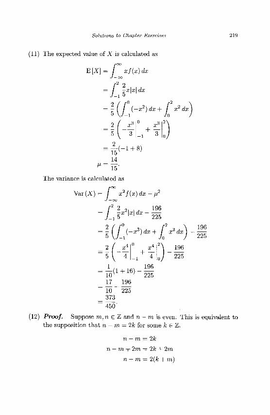
Solutions to Chapter Exercises 219
(11) The expected value of X is calculated as
/
oo xf{x) dx
-OO
r 2
2 ' '° 5
xlxl da;
-x2) da; -
M
!i _2_
15 14 15
l
" 3
jf" da;
ar
( -1 + 8)
The variance is calculated as
/
oo x2 f(x) dx - ii2
-OO
L 2
5
- x 2 | a ; | dx • l 5
196 225
f / (-x3)dx+ / a;3 da;) -196 225
x* "T +
196 225
= 1 ( 1 + 1 6 ) - ^ 10 V ; 225 17 196
~ 10 ~~ 225 _ 373 ~ 450'
(12) Proof. Suppose ra,neZ and n - m i s even. This is equivalent to the supposition that n — m = 2k for some fceZ.
n — m = 2k
n — m + 2m = 2k + 2m
n + m = 2(k + m)
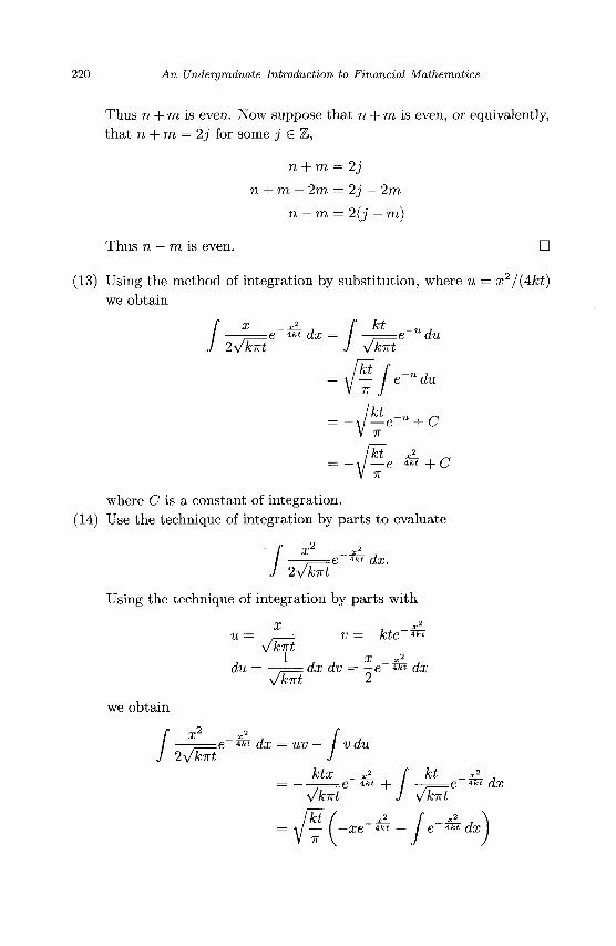
220 An Undergraduate Introduction to Financial Mathematics
Thus n + 77i is even. Now suppose that n + TO is even, or equivalently, that n + TO = 2j for some j € Z,
n + m = 2 j
n + m — 2m = 2j — 2m
n — m = 2 (J — TO)
Thus n — TO is even. • (13) Using the method of integration by substitution, where u = x2 /{Akt)
we obtain
/ — ; e 4fct dx =
J 2Vknt J
kt
/knt :e-udu
?/- du
e~u + C
where C is a constant of integration. (14) Use the technique of integration by parts to evaluate
/ -e 4ht dx.
2Vkirt
Using the technique of integration by parts with
X , _ j £ i v = —kte lkt
vknt 1 x i 2
du = , dx dv = — e~"« dx
we obtain
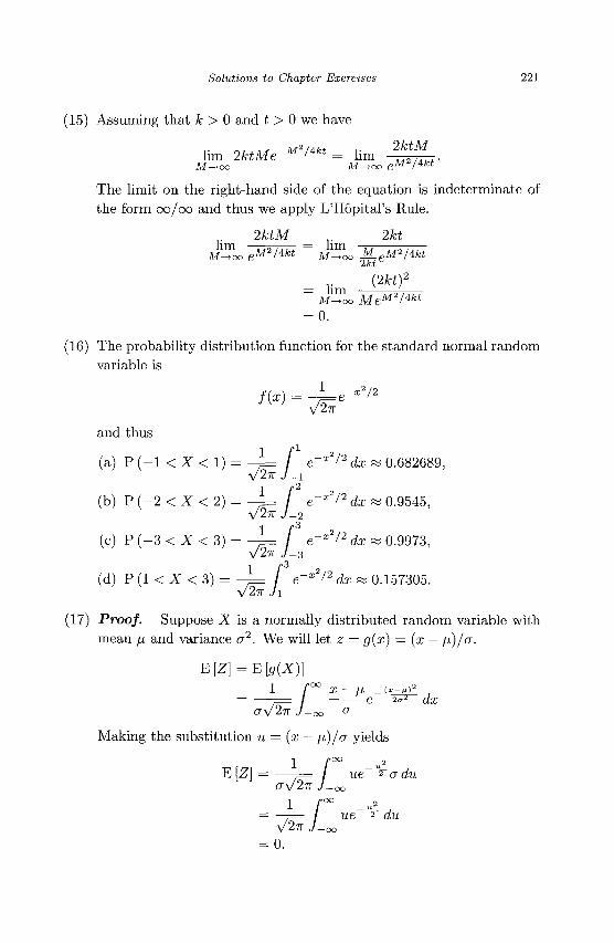
Solutions to Chapter Exercises 221
(15) Assuming that k > 0 and t > 0 we have
2ktM lim 2ktMe~M '4kt = lim
M->oo M ^ o o eM2/ikt '
The limit on the right-hand side of the equation is indeterminate of the form oo/oo and thus we apply L'Hopital's Rule.
2ktM ,. 2kt lim ,,,, , , , , = lim M ^ o o eM2/4fct M -*oo M eM2/4fct
2/ct
- lim ^ M—KX
MeM2/4kt
= 0.
(16) The probability distribution function for the standard normal random variable is
and thus 1 f1
(a) P ( - K X < 1) = - = / e~x2/2 dx « 0.682689, V27T J _ i
1 Z"2
(b) P ( -2 < X < 2) = — = / e"x 2 /2 da; « 0.9545, V27r 7-2
1 f3
(c) P ( -3 < X < 3) = - = / e~x^2 dx « 0.9973, 1 /""
(d) P (1 < X < 3) = - 7 = / e-^2/2 dx « 0.157305. V 27T J l
(17) Proof. Suppose X is a normally distributed random variable with mean \i and variance a2. We will let z = g{x) = (x — [i)jo.
E[Z}=E[g(X)}
l r° aV2~n J-(
X — fl _{x-lx)-1
e 2<T dx a
Making the substitution u = (x — fi)/a yields
E[Z]
=
=
1
aV2n . 1 /
0.
/•oo / we
J —oo r>oo
- o o ue
u 2
u 2
"2" tiu
du
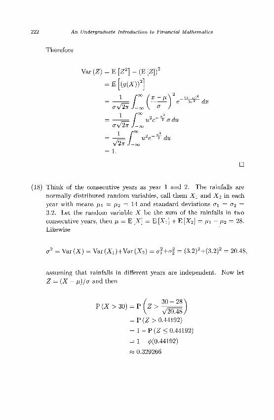
222 An Undergraduate Introduction to Financial Mathematics
Therefore
Var(Z) = E[Z 2 ] -{E[Z})2
= E [(g(X))2]
aV2n i -oo V °" /
D
(18) Think of the consecutive years as year 1 and 2. The rainfalls are normally distributed random variables, call them X\ and X2 in each year with means £ti = /Z2 = 14 and standard deviations o\ = 01 = 3.2. Let the random variable X be the sum of the rainfalls in two consecutive years, then JJ, = E [X] = E [Xi] + E [X2] = Mi + M2 = 28. Likewise
a2 = Var (X) = Var (Xi)+Var (X2) = (J\+<J\ = (3.2)2+(3.2)2 = 20.48,
assuming that rainfalls in different years are independent. Now let Z = (X — fi)/a and then
/ 3 0 - 2 8 \ P(Z>30) = P ( Z > 7 = )
= P (Z > 0.44192)
= 1-P{Z < 0.44192)
= 1 - 0(0.44192)
« 0.329266
Solutions to Chapter Exercises 223
(19) Let the random variable X represent the ratio of consecutive days selling prices of the security.
p {X > 1) = P ( l n X
= p(z>
= p(z>
= P(Z>-
« 0.57926
>0 )
*-¥) 0 - 0 . 0 1
0.05 -0.20)
Thus the probability of a one-day increase in the price of the security is approximately 0.57926. Consequently the probability of a one-day decrease in the price of the security is approximately 1 — 0.57926 = 0.42074. The probability of a four-day decrease in the selling price of the security is
P(X4 < 1) = P ( 4 1 n X < 0 )
p | Z < ° - a 0 4
0.10
P {Z < -0.40)
0.344578.
(20) Since X is uniformly distributed on [a, b] its probability distribution function is
/•/ \ f TT— H a < x < b, f(X) = ) b~a - -0 otherwise
We will make use of Theorem 3.9.
f J X
1 if x < a
fit) dt={ |Ef if a < ^ < 6 0 if x > b
224 An Undergraduate Introduction to Financial Mathematics
Thus
E [(X - K)+] = j°° (J°° f(t) dt\ dx
JbK^adx ifa<K<b
0 if K > b
^ - K UK <a
if a < K <b 2(b-a) 0 if K > b
(21) By definition
V27T j - o o
Now we make the substitution u = —t.
1 rXe-*'/*dt= 1
-''Vdt.
~u2/2du 2 T T ,
2nJx
V2TT
4>{-x) = 1 - 4>{x)
-u 2 /2 du
(22) Proof. Using the definition of variance and Eqs. (3.15) and (3.17) we have
Var ({X - K)+)
E ((X-i^)+)2 - (E[(X-X)+]) 2
((/* - 2K)2 + a2^ -A {V-2K\ a. (M-2X)a p _ ( M _ 2 J , )V2^ 2TT
Br^'^-M^))' D
Solutions to Chapter Exercises 225
(23) Proof. Using the definition of variance and Eqs. (3.16) and (3.19) we have
Var ({X - K)+)
E ((X-K)+f -(E[(X~K)+}Y
= e2(M+<j2)0(™ + 2a) - 2Ke>M+a2/2(f)(w + a) + K2(j>(w)
/eM+a2/20 (w + a)- K<j) {w)Y
where w = [ji — h\K)/a. •
B.4 The Arbitrage Theorem
(1) Converting from the odds against to probabilities that the outcomes may occur produces a table of probabilities like the following:
Outcome Probability
A B C
Since the probabilities sum to ^§ > 1 the Arbitrage Theorem guarantees the existence of a betting strategy which yields a positive payoff regardless of the outcome. Suppose we wager x, y, and z on outcomes A, B, and C respectively. The payoffs under different winning scenarios are listed in the next table.
Winning Outcome A B C
-2x + y + z x — 2>y + z x + y — z
Payoff
We need only find values for x, y, and z which make the three expressions in the column on the right positive. By inspection we can see that x = 1, y = 1, and z = 2 is one solution to this set of inequalities.
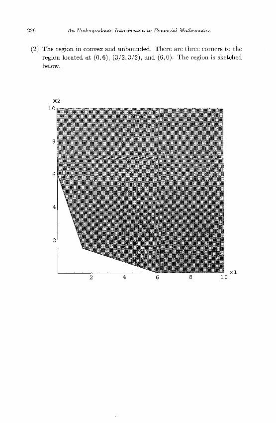
226 An Undergraduate Introduction to Financial Mathematics
(2) The region in convex and unbounded. There are three corners to the region located at (0,6), (3/2,3/2), and (6,0). The region is sketched below.
x2 1 0
1 0 x l
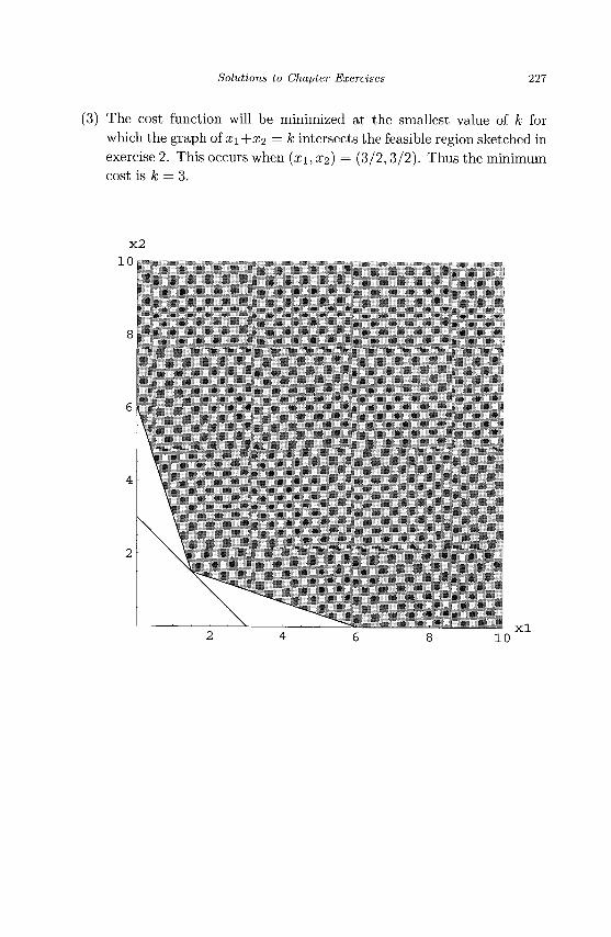
Solutions to Chapter Exercises 227
(3) The cost function will be minimized at the smallest value of k for which the graph of x\ +x2 = k intersects the feasible region sketched in exercise 2. This occurs when (xi, x2) = (3/2,3/2). Thus the minimum cost is k = 3.
x2 10.
— ^ 10
x l
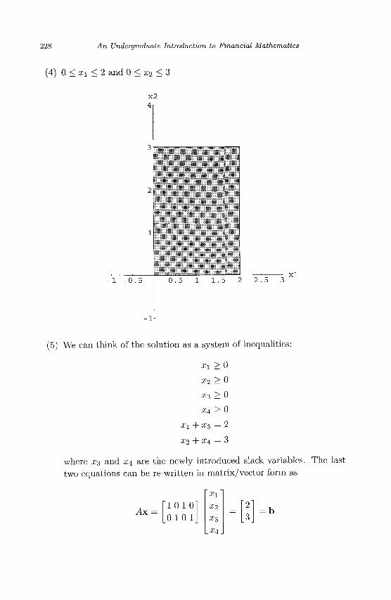
228 An Undergraduate Introduction to Financial Mathematics
(4) 0 < xi < 2 and 0 < x2 < 3
x 2
4r
x l - 0 . 5
- 1 L
0 . 5 1 . 5 2 . 5
(5) We can think of the solution as a system of inequalities:
xi > 0
x2 > 0
x3 > 0
xA > 0
x2 + £4 = 3
where x3 and £4 are the newly introduced slack variables. The last two equations can be re-written in matrix/vector form as
Ax "10 10" 0 1 0 1_
' Xl'
x2
£3 _X\_
= "2" 3
Solutions to Chapter Exercises 229
(6) Let vector c = (1,1,2) and x = (xi,X2,x3). The problem as stated
can be thought of as the primal problem:
Minimize: c • x subject to Ax = [ 1 2 3] x = 15 = 6.
This is equivalent to the dual problem:
Maximize: by = 15y subject to yA < c.
From the inequality constraint in the dual problem we know tha t
y < 1/2. Thus the maximum value of 15y is 15/2. Thus the minimum
value of c • x = 15/2.
(7) Let vector c = (0 ,7 ,9 ,0) and x = {XI,X2,X3,XA). The problem as
stated can be thought of as the primal problem:
Minimize: c • x subject to Ax =
This is equivalent to the dual problem:
Maximize: y • b = [yi y2) b subject to yA < c.
The constraint inequality for the dual problem is equivalent to the
following system of linear inequalities.
2/i < 0
2/i + 2/2 < 7
2/1 + 2/2 < 9
2|/2 < 0
The first and last of these inequalities imply strict inequality in the
second and third. Thus by Theorem 4.2 x2 = x-$ = 0. Therefore the
primal problem can be restated as the following:
" 1 1 1 0 "
|_0 1 1 2\ x =
"5"
ll\
Minimize: (0, 0) • (xi, X4) subject to 1 0
0 2 X\
X4
5 1
Thus the minimum value of the cost function is 0 and occurs where
( z i ,x 2 , x 3 , a :4 ) = (5 ,0 ,0 ,1 /2 ) .
(8) In this case we must introduce a slack variable X4 to convert the
inequality constraint in the primal problem to an equality constraint.
Thus we want to think of the primal problem as:
Minimize x\JrX2~Vxz subject to 2x\+X2 = 4 and £3 + 2:4 = 6 with xt > 0 for i = 1 ,2,3,4.
230 An Undergraduate Introduction to Financial Mathematics
If we define the following vectors and matrix
(1,1,1,0), x = (x1,X2,x3,x4}, A 2 1 0 0 0 0 11
and b = (1,6),
then the primal problem is the one of minimizing c • x subject to Ax. = b and x > 0. The dual to this problem is the one of maximizing y • b subject to yA < c where y = (2/1,2/2)- This is equivalent to maximizing y1 + 62/2 subject to the system of inequalities
2yi < 1
2/i < 1
2/2 < 1
2/2 < 0 .
(9) Paying attention to the inequality constraints of the dual problem indicates that 2/1 < 1/2 and 2/2 < 0. Thus by Theorem 4.2 X2 = 2:3 = 0. We can also see that the maximum of y • b will be 1/2. This is also the minimum of the primal problem. However, we can also solve the primal problem directly after re-writing it as
Minimize: (1,0) • (£1,0:4) subject to
From the constraint equation we see that now (2:1,2:2,£3,£4) (2,0, 0, 6) and the minimum value of the cost function is 2.
(10) Written in matrix/vector form this dual problem becomes:
Maximize y • b = (2/1,2/2,2/3) • (2,0, 4) subject to
"20 ' 0 1
Xi
X4 =
"4" 6
yA = [2/1 2/2 2/3.
" 1 0" - 1 1
. ° 2. <
' 1 " - 1
Thus the primal problem is
Minimize c • x = (1, —1) • {x\,x2) subject to
Ax.--' 1 0" - 1 1
. ° 2.
Xi
. X 2 . =
"2" 0
_4_ = b .
(11) Find the solutions to the primal and dual problems of exercise 10. We can see from the constraint equation for the primal problem that x = (2:1, X2) = (1, !)• Thus the minimum value of the cost function is
Solutions to Chapter Exercises 231
c • x = (1, — 1) • (1,1) = 0. Therefore the maximum of the dual problem is likewise 0.
B.5 Random Walks and Brownian Motion
(1) If / is a continuous, twice differentiable function whose second derivative is 0 on the interval [0, A], then / must be a linear function of the form f(x) = ax + b where a and b are constants. Since /(0) = 0 then 6 = 0. Since f(A) = 1 then a = 1/A Thus we have f(x) = x/A. This agrees with our earlier derivation of exit probabilities for the discrete, symmetric random walk.
(2) If g is a continuous, twice differentiable function whose second derivative is —2 on the interval [0, A], then g must be a quadratic function of the form g(x) — ax2 + bx + c where a, b, and c are constants. Since g(0) = 0 then c = 0. Since g"(x) = —2 then a = — 1 which implies g(x) = x(b — x). Since g(A) = 0 then b = A. Thus we have g(x) = x(A — x). This agrees with our earlier derivation of the conditional stopping times for the discrete, symmetric random walk.
(3) This is an example of a symmetric random walk. Because of the spatial homogeneity property of the random walk, the desired probability is equivalent to determining the probability that a symmetric random walk initially in state 5(0) = 50 will attain a value of 75 while avoiding the absorbing boundary at 0. Using Theorem 5.1, the probability is p75(50) = 50/75 = 2/3.
(4) As in exercise 3 the exit time is equivalent to the exit time of a symmetric random walk on the discrete interval [0,75] which begins in the state 5(0) = 50. Using Theorem 5.2, the probability is fi0,75(50) = 50(75 - 50) = 1250.
(5) As in exercise 3 the conditional exit time is equivalent to the conditional exit time of a symmetric random walk on the discrete interval [0, 75] which begins in the state 5(0) = 50. We must set up and solve a tridiagonal linear system of the form shown in Eq. (5.15) where A = 75. This is best done with the aid of a computer or calculator since the linear system contains 76 unknowns (really only 74 since the boundary conditions are known). In this case Z50 = 6250/9 « 694.444. Thus Q7s(50) = 3125/3 « 1041.67.
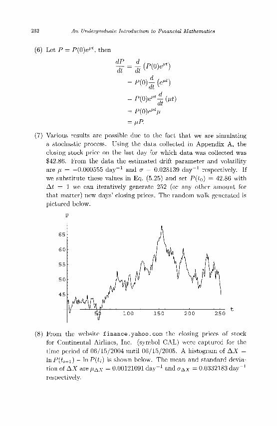
232 An Undergraduate Introduction to Financial Mathematics
(6) Let P = P(0)e"<, then
dP_ dt
d ~d~t
(P(OK')
= P(0)e" t | (M i )
= P(0)eMV = tiP.
(7) Various results are possible due to the fact that we are simulating a stochastic process. Using the data collected in Appendix A, the closing stock price on the last day for which data was collected was $42.86. From the data the estimated drift parameter and volatility are \x = -0.000555 day - 1 and a = 0.028139 day - 1 respectively. If we substitute these values in Eq. (5.25) and set P(to) = 42.86 with At = 1 we can iteratively generate 252 (or any other amount for that matter) new days' closing prices. The random walk generated is pictured below.
(8) From the website finance.yahoo.com the closing prices of stock for Continental Airlines, Inc. (symbol CAL) were captured for the time period of 06/15/2004 until 06/15/2005. A histogram of AX = lnP(ij+i) — lnP(ij) is shown below. The mean and standard deviation of AX are fiAX = 0.00121091 day"1 and aAX = 0.0332183 day"1
respectively.
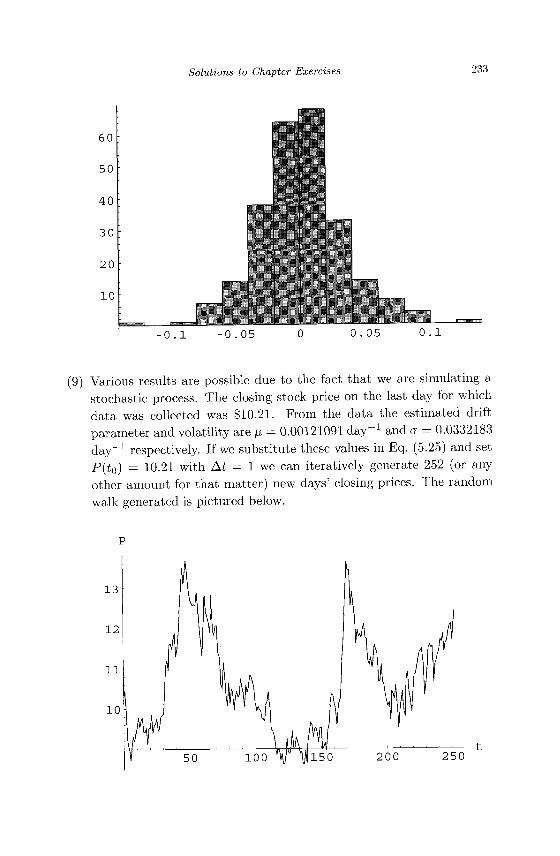
Solutions to Chapter Exercises 233
60
50
40
30
20
10
•
l 1 . - 0 . 1 . 1
(9) Various results are possible due to the fact that we are simulating a stochastic process. The closing stock price on the last day for which data was collected was $10.21. From the data the estimated drift parameter and volatility are \i = 0.00121091 day"1 and a = 0.0332183 day~* respectively. If we substitute these values in Eq. (5.25) and set P(£0) = 10.21 with At = 1 we can iteratively generate 252 (or any other amount for that matter) new days' closing prices. The random walk generated is pictured below.
2 5 0
234 An Undergraduate Introduction to Financial Mathematics
(10) If F = F{y, z) and f(x) = F(y0 + xh, z0 + xk) then
dv dz f'(x) = Fy(y0 + xh, z0 + xk)— + Fz(yQ + xh, z0 + xk) —
= Fy(y0 + xh, z0 + xk) — [y0 + xh]
+ Fz(y0 + xh, z0 + xk)— [z0 + xk] ax
= Fy(y0 + xh, z0 + xk)h + Fz(y0 + xh, z0 + xk)k
/ ' (0) = Fy(y0, z0)h + Fz{y0, z0)k.
Differentiating once again produces
dij dz f"{x) = Fyy(y0 + xh, z0 + xk)h— + Fyz(y0 + xh, z0 + xk)h—
dij dz
+ Fzy(y0 + xh, z0 +xk)k— + Fzz(y0 + xh, z0 + xk)k—~
= hFyy(y0 + xh, z0 + xk)— [y0 + xh]
+ hFyz(y0 + xh, z0 + xk)— [z0 + xk]
+ kFzy(y0 + xh, z0 + xk)— [y0 + xh)
+ kFzz (y0 + xh, z0 + xk) — [z0 + xk] ax
= h2Fyy(yo + xh, z0 + xk) + 2hkFyz(y0 + xh, z0 + xk)
+ k2Fzz(y0 + xh, z0 + xk)
/"(0) = h2Fyy{y0,z0) + 2hkFyz(y0,z0) + k2Fzz(y0,z0) By definition the Taylor remainder of order 3 for f(x) is Rs(x) — ) „
-x for some a between 0 and x. If we notice the binomial / " ' ( « ) , 3
3! coefficient pattern among the partial derivatives in the first and second derivatives of f(x) then we can readily see that
f'"(x) = h3Fyyy(yo + xh, z0 + xk) + 3h2kFyyz(y0 + xh, z0 + xk)
+ 3hk2Fyzz(y0 + xh,z0 + xk) + k3Fzzz(y0 + xh,z0 + xk).
From this expression we may directly determine the Taylor remainder of order 3.
Solutions to Chapter Exercises 235
(11) If we apply Ito's Lemma with a(P,t) = /iP and b(P,t) = aP and Y = Pn, then
dY = (nPnP™-1 + -(aP)2n{n - l)Pn~A dt + aPnPn~x dW(t)
nfJLpn + n(n ~ 1> pn\ dt + n(Jpn d w ^
(12) If we apply Ito's Lemma with a(P,t) = fiP and b(P,t) = aP and Y = In P, then
dY fiP
M +
" l n
~PJ
a2N
+ \(<rPf
] dt + a dW it)
)dt + aP "1
dW(t)
B.6 Options
(1) Suppose the value of an American put option is Pa and that Pa < Pe, the value of a European put option on the same underlying security with identical strike price and exercise time. An investor could sell the European put option and buy the American put option and invest the net positive cash flow of Pe — Pa in a risk-free bond at interest rate r. At the exercise time, in either the case where the owner of the European put exercises the option or not, the investor has a portfolio with value (Pe - Pa)e
rT > 0.
(2) The net payoff will be the quantity (S(T) - K)+ - C where K = 60 and C = 10. The payoff is plotted below.
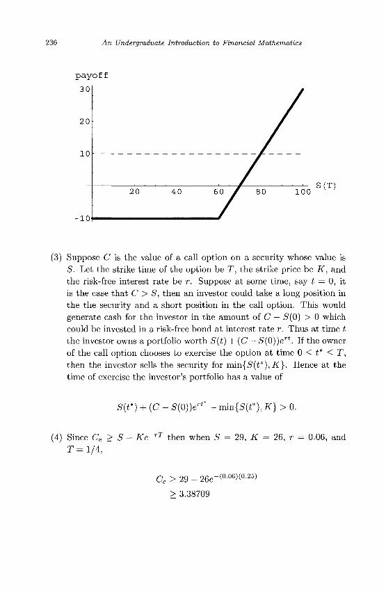
236 An Undergraduate Introduction to Financial Mathematics
payoff
30f
20
10
•10
20 40 60 80 100 S(T)
(3) Suppose C is the value of a call option on a security whose value is S. Let the strike time of the option be T, the strike price be K, and the risk-free interest rate be r. Suppose at some time, say t = 0, it is the case that C > S, then an investor could take a long position in the the security and a short position in the call option. This would generate cash for the investor in the amount of C — 5(0) > 0 which could be invested in a risk-free bond at interest rate r. Thus at time t the investor owns a portfolio worth S(t) + (C — S(0))ert. If the owner of the call option chooses to exercise the option at time 0 < t* < T, then the investor sells the security for min{5(i*), K}. Hence at the time of exercise the investor's portfolio has a value of
S(f) + (C - S'(0))ert* - min{S{t*),K} > 0.
(4) Since Ce > S - Ke~rT then when S = 29, K = 26, r = 0.06, and T = 1/4,
Ce > 29 - 26e-(°-06»0-25)
> 3.38709
Solutions to Chapter Exercises 237
(5) Suppose S = 31, T = 1/4, Ce = 3, K = 31, and r = 0.10 then according to the Put-Call Parity Formula in Eq. (6.1):
Pe + S = Ce + Ke~rT
Pe + 31 = 3 + 31e-(o.io)(o.25)
Pe = 3 + 31 e-(°-1 0»0-2 5)-31
Pe = 2.23461
(6) Suppose S = 31, T = 1/4, Ce = 3, Pe = 2.25, and r = 0.10 then according to the Put-Call Parity Formula in Eq. (6.1):
Pe + S = Ce + Ke~rT
2.25 + 31 = 3 + ^e-(0-io)(o.25)
2.25 + 31 - 3 = Ke-(o.io)(o.25)
K = (2.25 + 31-3)e(°-10)(°-25)
K = 31.0158
(7) Suppose T = 1/6, if = 14, S = 11, and r = 0.07 then according to the Put-Call Parity Formula in Eq. (6.1):
Pe = Ce-S + Ke~rT
> -S + Ke~rT
= _H + l 4 e - ( 0 - 0 7 ) / 6
= 2.83762
(8) An investor could take a long position in the put option and the security and short position in the call option while borrowing, at the risk-free rate, the strike price of the options. This generates an initial cash flow of
K + Ce - Pe - S = 30 + 3 - 1 - 31 = $1.
This amount could be invested at the risk-free rate until the strike time arrives. At t = 3 months if S(3) > 30 = K, then the call option will be exercised at the investor cancels all positions with a portfolio worth
le(o.io)(o.25) + 3 0 _ 30e(o.io)(o.25) = $ 0 . 2 6 5 8 6 2 > 0.
238 An Undergraduate Introduction to Financial Mathematics
If the call option finishes out of the money, the investor exercises the put option and finishes with a portfolio worth again
le(o.io)(o.25) + 3 0 _ 30e(o.io)(o.25) = $0.265862 > 0.
(9) If fi(S,t) and f2(S,t) both satisfy Eq. (7.5) then
rfi = h,t + \v2S2h,ss + rSfhS and
rh = h,t + \o2S2f2,ss + rSf2<s.
Therefore if c\ and c2 are real numbers
rcifi = c i / M + - C T 2 5 2 C I / I I S S + rScifi^s and
rc2f2 = c2f2,t + 7jV2S2c2f2,ss +rSc2f2,s-
Adding left-hand sides and right-hand sides of the previous two equations produces
rcifi + rc2f2 = c i / i , t + -(r2S2c1fi!ss + rScifi,s
+c2f2,t + -^cr2S2c2f2tss + rSc2f2,s
r(cifi + c2/2) = (ci/i , t + c2f2,t) + ~cr2S2(c1fl!ss + c2f2,ss)
+rS(cifitS + c2f2,s)
= (ci/i + c2h)t + \<?2S2{Clh + c2f2)Ss
+rS(c1f1+c2f2)s
rf = ft + \cr2S2fss+rSfs.
(10) At time t = T the payoff of the European put option will be
max{0, K - S(T)} = (K - S(T))+,
thus F(S,T) = {K - S(T))+. If the stock is worthless (i.e., 5 = 0) then the put option will be exercised and F(Q, t) = K. As the price of the stock increases toward infinity the put option will not be exercised and thus linis^oo F(S, t) = 0.
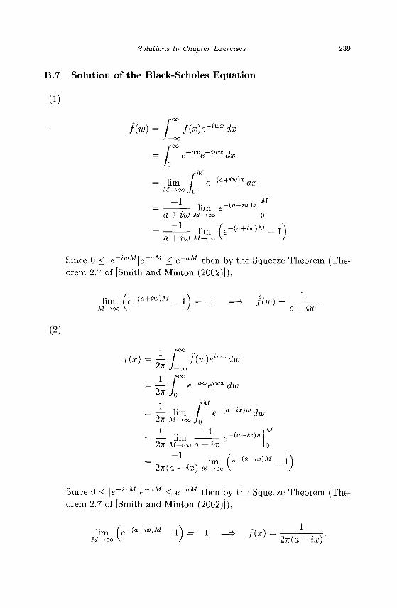
Solutions to Chapter Exercises 239
B.7 Solution of the Black-Scholes Equation
(1)
/
OO
-oo
: dx
/ e -^e - ™* dx Jo
pM
lim / e-(°+,u' ) : , : dx M^COJQ
~l lim e-(0+™)* a + iw M- oo
M
0
_ 1 lim (e-(°+™)M a + 2W M-^oo
Since 0 < | e - ™ M | e - a M < e~aM then by the Squeeze Theorem (The
orem 2.7 of [Smith and Minton (2002)]),
lim (e-(*+iu)M _A fH a + iw
(2)
fix) = -^ J°° /Me™*
2TT
dw
e-awelwx dw
—— lim 27T M^oc
M
-1
-(a-ix)™ d w
— lim 27r M- oo a — ix
lim
-(o — ix)w M
27r(a — ix) M^OO (e-(a-ix)M _ A
Since 0 < \e~ixM\e-^
aM < e~aM then by the Squeeze Theorem (Theorem 2.7 of [Smith and Minton (2002)]),
lim fe-(«-«)M _ A = _i => f(x) = 27r(a — ix)
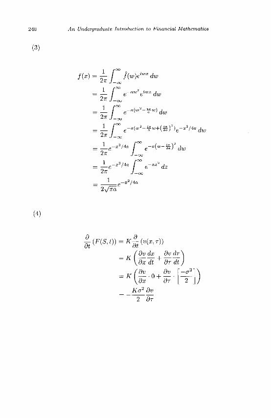
240 An Undergraduate Introduction to Financial Mathematics
(3)
(4)
f(x) = ^ l f(^ywxdw
1 2^
e-aw &lWx dw
-a(w*-i*w) d w
2W_, - r e-^^+i^e-^^dw !TT J-oo 2TT
1 r°° J_e-*2/4a f e- <w-£¥ dw
2TT
1
-z 2 /4a / e~az- dz
2\/Tra -x2/4a
^(F(S,t)) = K^(v(x,r))
( dv dx dv dr \dx dt dr dt /dv dv \dx dr
Ka2 dv 2~lfr
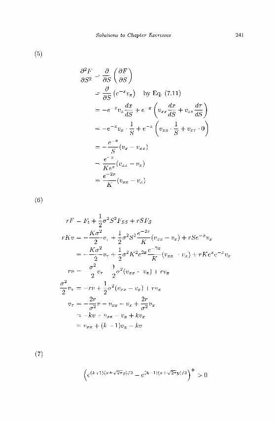
Solutions to Chapter Exercises
d2F d (dF OS2 dS V dS
d gg{e-xVx) by Eq. (7.11)
_„ dx _T ( dx dr — e Vr h e Vr-r h Vrr xdS \ xxdS dS
-e~xvx • — + e~x I vxx • - + vXT • 0
e -
e ^ ^ - j f e x ^
g-2a;
^xa: J
-vx)
-Vx)
rF = Ft + ^a2S2Fss + rSFs
Ka2 1 e~2x
rKv = — i v + ^2S2—j-^{vxx - vx) + rSe~xvx
Ka2 1 e_2a:
ff2 1 2,
rv = ~YVT + 2a ^Vxx ~~ Vx> + rVx
°2 l 2, —vT = -rv + -a (vxx - vx) + rvx
2r 2r Vr = ?V + Vxx -Vx + ~^Vx
az a2-= -kv + vxx -vx + kvx
= vxx + {k- l)vx - kv
(e(k+l)(x+V2^y)/2 _ e{k~l)(x+^2^y)/2\+ > Q

242 An Undergraduate Introduction to Financial Mathematics
if and only if
(fc+l)0+V^n/)/2 ^ (fc-l)(:H-v/2?2/)/2 > e ex+V2ry ^ ^
x + y/2ry > 0
y > -I IT
(8) By the result of exercise 7 we know that
1 /2TT
(>+D )(a;+V2?v)/2 _ p(k-l)(x+V2Ty)/2\+ -y2/2
V27T J-X/V2T
(e{k+l)(x+-j2^y)/
'dy
2 _ . ( f c - l X x + V ^ M p-y2/2
1 0[(k+l)(x+V2^y)-y2]/2 _ p[(k-l)(x + ^y)-y2}/2
•dy
dy >2ll J-X/V2r
Completing the square in the exponents present in the integrand yields
y2 - y/2r(k ± l)y - (k ± l)x
2 / s - „ , ^ ( f c ± l ) 2 r \ ( fc± l ) 2 r ., , _ y2 - V^(fc ± l)j/ + ^ ^— J - i ^ (/c ± l)x
(fc±l)v /2 :f\ (k±l)2
(k±l)x
Thus the integral in Eq. (7.31) becomes
X/V2T
<v-
-{y-
{k + l)V2^^2 / 0 (fc + 1) ) V 2 e ^ 4 L J : + ( fe+1W2dy
(fc-l)y/2T ^2 / n ( f c - l )^T
C/V2T
e(fc+l)2r/4+(fc+l)z/2 oo
1 ) 2 / 2 ei ^ ^ + (fc-l)x/2dy
/2TT
= (fc-l)2r/4+(fc-l)z/2
-(y-^¥^f/2dy
x/V2r
-(y- (k-l)V2¥^2 r/2 dy V27T J-X/V2T
(9) If we let w = -y + \{k + l)-v/2r, then dw = -dy. When y = -x/V^r
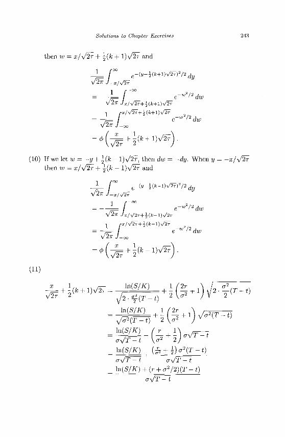
Solutions to Chapter Exercises 243
then w - X/V2T+ \(k + l ) \ /2r and
V27T J-x/y/2^
-w2'2dw 27T Jx/V^+^ik+l)^
/ e-w'2dw J — oo
{wA{k+l)^)' (10) If we let w = -y+\(k-l)y/2r, then dw = -dy. When y = -xjyf^r
then w = x/y/2~r + |(fc — 1 )V^T : and
1 /-oo
: L / e-(y- | ( fc- i )v^) 2 /2 d 2 /
27T J-x/^/2^ 1 /• —oo
i= / e - 2 / 2 d w 27r A / v ^ + ^ f c - i ) ^ ^
/ e~w I2 dw J —oo
(11)
(j= + i(t-i)vS).
! / . ^ /TT- ln(S7in 1 / 2 r i /„ « / m ^
7 ' 2 ( H 1 ) ^ = ^= + 2b + l h / 2 ' T ( r - t )
ln(5/if) 1 / 2 r \ ^
aVT^t \a2 2t
HS/K) [ ( ^ + l ) g 2 ( r _ t )
ay/T-t ay/T-t
ln(S/K) + (r + a2/2)(T-t)
ay/T-t
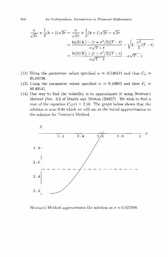
244 An Undergraduate Introduction to Financial Mathematics
J IT &
1 (fc + l ) V 2 r - V 2 r
IIT r ln{S/K) + (r + a2/2)(T-t)
ay/T-t ln(S/K) + {r + a2/2)(T-t)
2 - y ( T - t )
WT-t
(12) Using the parameter values specified w « 0.536471 and thus Ce « $5.05739.
(13) Using the parameter values specified w « 0.16662 and thus Pe w $6.40141.
(14) One way to find the volatility is to approximate it using Newton's Method (Sec. 3.2 of [Smith and Minton (2002)]). We wish to find a root of the equation Ce(a) = 2.50. The graph below shows that the solution is near 0.80 which we will use as the initial approximation to the solution for Newton's Method.
2 . 8
2 . 6
2 . 4
2 . 2
Newton's Method approximates the solution as a « 0.827888.
Solutions to Chapter Exercises 245
(15) If f(S,t) = S, then fs = 1, fss = 0, and ft = 0. Thus
rf = ft + \cr2S2fss + rSfs
rS = 0+ ]-a2S2 -0 + rS
rS = rS.
Therefore the price of the security itself solve the Black-Scholes partial differential Eq. (7.5).
B.8 Derivatives of Black-Scholes Option Prices
(1) Using Eq. (8.3) with S = 300, K = 310, T = 1/4, t = 0, r = 0.03, and a = 0.25 we have
w = -0.139819
6 = -33.281
(2) To find O for a European put option we will make use of the Put/Call parity formula (Eq. (6.1)) and Eq. (8.3). According to the Put/Call parity formula,
dP 3C ^ _ r r r _ 0
Substituting the expression already found for ^ in the right-hand
246 An Undergraduate Introduction to Financial Mathematics
side of this equation yields
dP _ Se~w I2 - Ke-rV-V-^-*^^ I2 (HS/K) _ 2
dt 2ay/2ir(T -t) \ T-t
- i f e - r ( T - * ) ( r4>{w - aVf~^t) ae-(w-aVT^iy/2
2^2ir(T-t) J
Se-^l2 - g e - r ( r - t ) - ( M - f f y ^ ) V 2 (MSIK) _ 2
2<ry/2Tv(T - t) \ T-t ~ r ~ a I2
crft'e-' '(T-t)-(w-<Tv /T^t)2/2 + ( i - 4>{w - CTVT - 1 ) )
Se-w2/2 (HS/K) 2
2^2n(T-t)
r - a2/2 2O^2TT{T - t) \ T - t
+ Kre-r(T-t)(j){aVT~^t - w)
Ke-r(T-t)-(w-*VT=tf/2 fl^S/K) , , \ / —7^r—k ~ r ° -a 2 +a)
2^2TT(T -1) \<j(T-t) ' ' )
Se~w2l2 (HS/K) r - 0-72
2ay/2Tr{T - t) \ T-t
+ Kre-r{T-t)4>{aVT~^t - w)
2a^2ir(T - t) \ T-t T + ° '
(3) Using Eq. (8.5) with 5 = 275, K = 265, T = 1/3, t = 0,r = 0.02, and a = 0.20 we have
w = 0.436257
6 = -15.3073
(4) According to Eq. (7.35)
HS/K) + (r + a2/2){T-t) w aVf~^t
Solutions to Chapter Exercises 247
which implies that
dw d
~dS = 'dS
_ _d_
~ dS
\n{S/K) + {r + a2/2)(T-t)
aVT^t ln(S/K)
1 d
aVT^tdS 1 d
ay/T=tdS 1 1
[HS/K)}
[In S - I n K]
ay/T^t S 1
aSVT^t
(5) Using Eq. (8.8) with S = 150, K = 165, T = 5/12, t = 0, r = 0.025, and a = 0.22 we have
w = -0.526797
A = 0.299167
(6) Using Eq. (8.9) with S = 125, K = 140, T = 2/3, t = 0, r = 0.055, and (j = 0.15 we have
w = -0.564706
A = -0.713863
(7) Using Eq. (8.11) with S = 180, K = 175, T = 1/3, t = 0, r = 0.0375, and a = 0.30 we have
w; = 0.321416
r = 0.0121519
(8) According to Eq. (7.35)
w_ HS/K) + {r + ^/2){T-t)
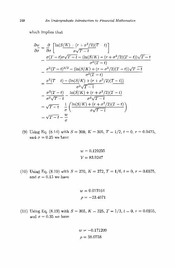
248 An Undergraduate Introduction to Financial Mathematics
which implies that
dw d da da
ln(S/K) + (r + a2/2)(T-t) ay/T^t
a{T - t)ay/T~^t - (ln{S/K) + (r + a2/2)(T - t))y/T^t
a2(T-
a2{T-
- tf'2
" * ) -
a2{T-t) -(ln(S/K) + (r + a2/2)(T-
a2(T-t) (HS/K) + (r + a2/2)(T-t))
t))y/T -1
a2VT^i a2{T-t) HS/K) + {r + a2/2)(T-t) a2y/T^t a2y/T=t
1 f\n(S/K) + (r + a2/2){T-t) y/T^t-- ,
a \ ay/T^t
(9) Using Eq. (8.14) with S = 300, K = 305, T = 1/2, t = 0,r = 0.0475, and a = 0.25 we have
w = 0.129235
V = 83.9247
(10) Using Eq. (8.19) with S = 270, K = 272, T = 1/6, t = 0, r = 0.0375, and a = 0.15 we have
w = 0.012164
p = -23.4071
(11) Using Eq. (8.19) with S = 305, K = 325, T = 1/3, t = 0, r = 0.0255, and a = 0.35 we have
w = -0.171209
p = 38.0758
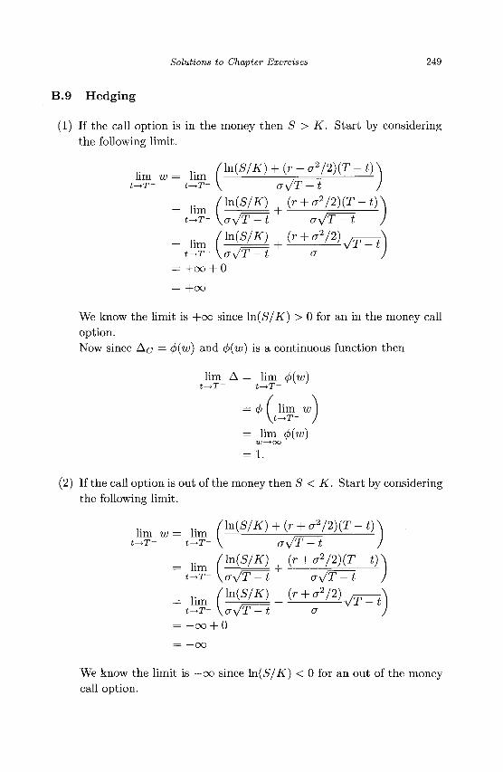
Solutions to Chapter Exercises 249
B.9 Hedging
(1) If the call option is in the money then S > K. Start by considering the following limit.
lim „ = lira (MW+iL+f/HKIzi) t _ T - t->T~ V OyjT -t
= l i m (HS/K) (r + ay2)(T-t) t^T- \ay/T^t (Ty/T-t
= lim (Msm + ir^yi)^ t^T- \ay/T-t a-
= +00 + 0
= + OO
We know the limit is +00 since \n(S/K) > 0 for an in the money call option. Now since Ac = 4>{w) an<A <fr(w) is a continuous function then
lim A = lim <b{w) t->T- t->T-
lim w t~>T~
= lim 4>(w) w—^oo
= 1.
(2) If the call option is out of the money then S < K. Start by considering the following limit.
n m u ; = l i m (HS/K) + (r+^/2)(T-t) t-T- t^T- V ay/T -t
= lim (WW 1 (r + v2/2)(T-t)\ t^T- \ay/T -t (Jy/T-t J
= lim (H^m+(r + aV2)vT^t t - r - \ay/T-t
= -OO + 0
= —00
We know the limit is —00 since \n(S/K) < 0 for an out of the money call option.
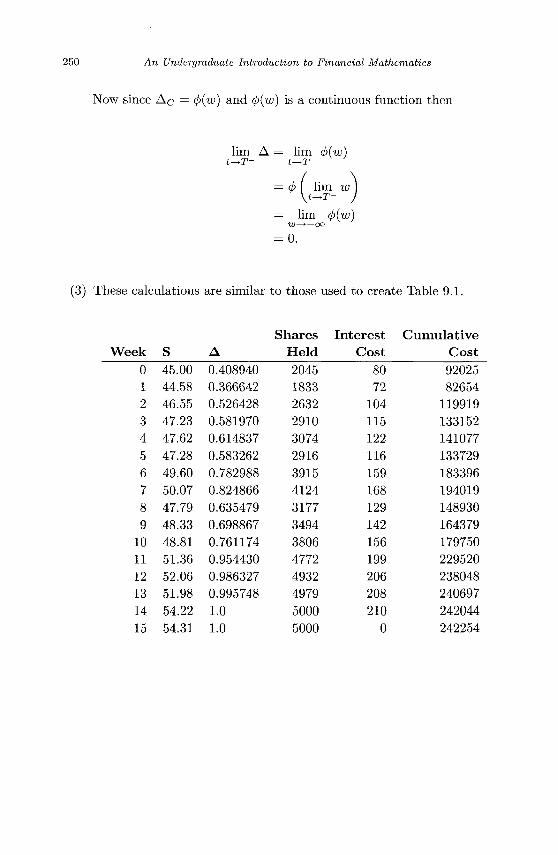
250 An Undergraduate Introduction to Financial Mathematics
Now since A c = 4>(w) and </>(«;) is a continuous function then
lim A = lim <j>(w) t->T- t->T-
= <p I lim w V - T - )
= lim <j>(w)
= 0.
(3) These calculations are similar to those used to create Table 9.1.
Shares Interest Cumulative ek 0 1 2 3 4 5 6 7 8 9 10 11 12 13 14 15
S 45.00 44.58 46.55 47.23 47.62
47.28 49.60 50.07 47.79
48.33 48.81 51.36 52.06 51.98 54.22 54.31
A 0.408940 0.366642
0.526428 0.581970 0.614837 0.583262
0.782988 0.824866 0.635479 0.698867 0.761174
0.954430 0.986327 0.995748
1.0 1.0
Held
2045 1833 2632 2910 3074
2916 3915 4124
3177 3494
3806 4772 4932 4979
5000 5000
Cost
80 72 104 115 122 116 159 168 129 142 156 199 206 208 210 0
Cost
92025 82654 119919 133152
141077 133729 183396 194019 148930 164379 179750 229520 238048 240697
242044 242254
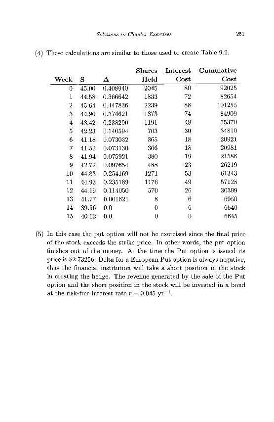
Solutions to Chapter Exercises 251
(4) These calculations are similar to those used to create Table 9.2.
Week
0 1 2
3 4
5 6 7 8 9 10 11 12 13 14
15
S
45.00
44.58
45.64
44.90
43.42
42.23
41.18
41.52
41.94
42.72
44.83
44.93
44.19
41.77
39.56
40.62
A
0.408940
0.366642
0.447836
0.374621
0.238290
0.140594
0.073032
0.073130
0.075921
0.097654
0.254169
0.235189
0.114050
0.001621
0.0 0.0
Shares
Held
2045
1833
2239
1873
1191
703 365 366 380 488 1271
1176
570
8 0 0
Interest
Cost
80 72
88 74
48 30 18 18 19 23 53 49 26 6
6 0
Cumulative
Cost
92025
82654
101255
84909
55370
34810
20921
20981
21586
26219
61343
57128
30399
6950
6640
6645
(5) In this case the put option will not be exercised since the final price of the stock exceeds the strike price. In other words, the put option finishes out of the money. At the time the Put option is issued its price is $2.73256. Delta for a European Put option is always negative, thus the financial institution will take a short position in the stock in creating the hedge. The revenue generated by the sale of the Put option and the short position in the stock will be invested in a bond at the risk-free interest rate r = 0.045 yr _ 1 .
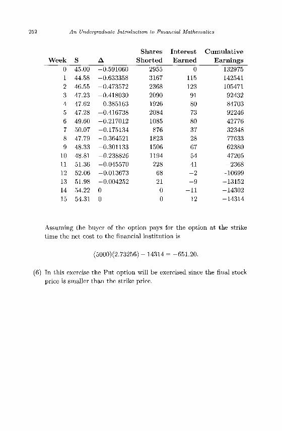
252 An Undergraduate Introduction to Financial Mathematics
ek 0 1 2 3 4 5 6 7 8 9 10 11 12 13 14 15
S 45.00 44.58 46.55 47.23 47.62
47.28 49.60 50.07 47.79 48.33 48.81 51.36 52.06
51.98 54.22
54.31
A -0.591060 -0.633358 -0.473572 -0.418030 -0.385163 -0.416738 -0.217012 -0.175134 -0.364521
-0.301133 -0.238826 -0.045570 -0.013673 -0.004252 0 0
Shares Shorted
2955 3167 2368 2090 1926 2084 1085 876 1823 1506 1194
228 68 21 0 0
Interest Earned
0 115 123 91 80 73 80 37 28 67 54 41 -2 -9 -11 -12
Cumulative Earnings
132975 142541 105471 92432 84703 92246 42776 32348 77633 62380 47205 -2368 -10699 -13152 -14302
-14314
Assuming the buyer of the option pays for the option at the strike time the net cost to the financial institution is
(5000)(2.73256) - 14314 = -651.20.
(6) In this exercise the Put option will be exercised since the final stock price is smaller than the strike price.

Solutions to Chapter Exercises 253
Week
0 1 2
3 4
5
6 7 8 9 10 11 12 13 14
15
S
45.00
44.58
45.64
44.90
43.42
42.23
41.18
41.52
41.94
42.72
44.83
44.93
44.19
41.77
39.56
40.62
A
-0.591060
-0.633358
-0.552164
-0.625379
-0.761710
-0.859406
-0.926968
-0.926870
-0.924079
-0.902346
-0.745831
-0.764811
-0.885950
-0.998379
-1.0
-1.0
Shares
Shorted
2955
3167
2761
3127
3809
4297
4635
4634
4620
4512
3729
3824
4430
4992
5000
5000
Interest
Earned
0 115 123
107 122
148
166 178 178 177 174
143 147 171 191 191
Cumulative
Earnings
132975
142541
124135
140676
170410
191166
205250
205386
204977
200540
165612
170024
196950
220595
221103
221294
At the strike time the financial institution must honor the Put option and cancel its short position in the stock. Thus the financial institution purchases 5000 shares of the stock at the strike price of $47 per share. This final transaction changes the holdings of the financial institution by
221294 - (5000)(47) + (5000)(2.73256) = -43.20.
(7) Let S = 85, K = 88, r = 0.055, and a = 0.17. We will let the number of four-month options be W4 and the number of six-month options be WQ. \iV represents the value of the portfolio consisting of a short position in the four-month options and a long position in the six-month options, then the value of the portfolio is V = w±C(S, | ) — WQC{S, | ) . Note that C(85, \) = 1.2972 and C(85, §) = 2.59313. Gamma for the
portfolio is
r = T4W4 — YQWQ
= 0.0474901^4 - 0.0390443w6.
Thus the portfolio is Gamma-neutral whenever W4 = 0.822155^6-
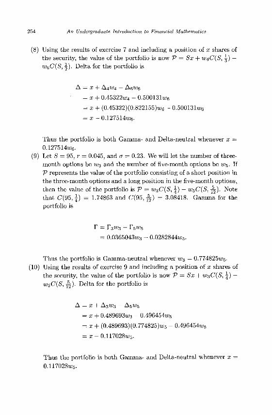
254 An Undergraduate Introduction to Financial Mathematics
(8) Using the results of exercise 7 and including a position of x shares of the security, the value of the portfolio is now V = Sx + WiC{S, | ) — WQC(S, \). Delta for the portfolio is
A = x + A4W4 — AeWQ
= x + 0.45322w;4 - 0.500131™6
= x + (0.45322)(0.822155)u;6 - 0.500131w6
= x - 0.127514u>6.
Thus the portfolio is both Gamma- and Delta-neutral whenever x = 0.127514w6.
(9) Let S = 95, r = 0.045, and a = 0.23. We will let the number of three-month options be u>s and the number of five-month options be W5. If V represents the value of the portfolio consisting of a short position in the three-month options and a long position in the five-month options, then the value of the portfolio is V = u>3C(S, | ) — w$C(S, ^ ) . Note that C(95, \) = 1.74863 and C(95, ^ ) = 3.08418. Gamma for the portfolio is
T = T3W3, - T5w;5
= 0.0365043w;3 - 0.0282844w5.
Thus the portfolio is Gamma-neutral whenever W3 = 0.7748251^5. (10) Using the results of exercise 9 and including a position of x shares of
the security, the value of the portfolio is now V = Sx + WsC(S, | ) — w$C(S, JTJ). Delta for the portfolio is
A = x + A3W3 - A5w5
= x + 0.489693^3 - 0.496454w5
= x + (0.489693) (0.774825)w5 - 0.496454W5
= x- 0.117028W5.
Thus the portfolio is both Gamma- and Delta-neutral whenever x =
0.117028^5-
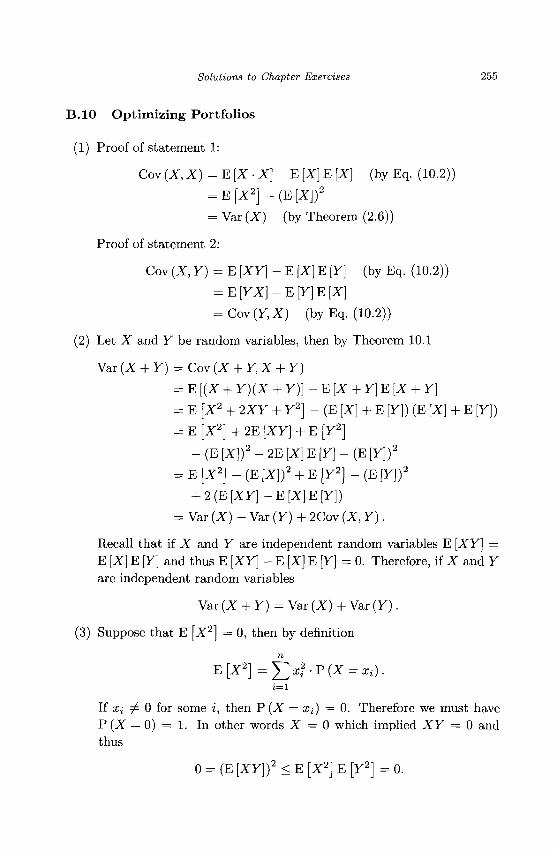
Solutions to Chapter Exercises 255
B.10 Optimizing Portfolios
(1) Proof of statement 1:
Cov (X, X) = E [X • X] - E [X] E [X] (by Eq. (10.2))
= E [ X 2 ] - ( E [ X ] ) 2
= Var (X) (by Theorem (2.6))
Proof of statement 2:
Cov (X, Y) = E [XY] - E [X] E [Y] (by Eq. (10.2))
= E [YX] - E [Y] E [X]
= Cov(y,X) (by Eq. (10.2))
(2) Let X and Y be random variables, then by Theorem 10.1
Var (X + Y) = Cov (X + Y, X + Y)
= E [(X + F) (X + Y)] - E [X + Y] E [X + Y]
= E [X2 + 2XY + Y2] - (E [X] + E [Y]) (E [X] + E [Y])
= E [X2] + 2E [XY] + E [y2]
- (E [X])2 - 2E [X] E [Y] - (E [Y]f
= E [X2] - (E [X])2 + E [y2] - (E [Y])2
+ 2 ( E [ X y ] - E [ X ] E [ y ] )
= Var (X) + Var (Y) + 2Cov (X, Y).
Recall that if X and Y are independent random variables E [XY] = E [X] E [Y] and thus E [XY] - E [X] E [Y] = 0. Therefore, if X and Y are independent random variables
Var (X + Y) = Var (X) + Var (Y).
(3) Suppose that E [X2] = 0, then by definition
V[X2]=J2*i-V(X = Xi)-i=l
If Xi ^ 0 for some i, then P (X = Xi) = 0. Therefore we must have P (X = 0) = 1. In other words X = 0 which implied XY = 0 and thus
0 = (E [XY]f < E [X2] E [y2] = 0.
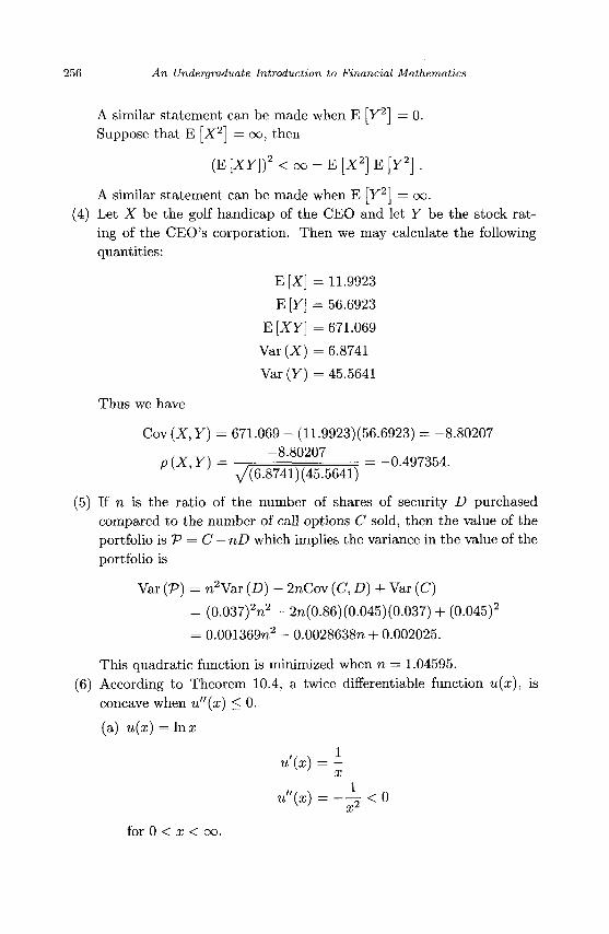
256 An Undergraduate Introduction to Financial Mathematics
A similar statement can be made when E [Y2] = 0. Suppose that E [X2] = oo, then
( E [ X y ] ) 2 < o o = E [ X 2 ] E [ y 2 ] .
A similar statement can be made when E [Y2] = oo. (4) Let X be the golf handicap of the CEO and let Y be the stock rat
ing of the CEO's corporation. Then we may calculate the following quantities:
E[X] = 11.9923
E [Y] = 56.6923
E[XY] =671.069
Var (X) = 6.8741
Var (Y) = 45.5641
Thus we have
Cov(X,Y) = 671.069- (11.9923)(56.6923) = -8.80207
p{x,Y) = , ~ 8 - 8 ° 2 0 7 = = -0.497354. ^(6.8741) (45.5641)
(5) If n is the ratio of the number of shares of security D purchased compared to the number of call options C sold, then the value of the portfolio is V = C — nD which implies the variance in the value of the portfolio is
Var (P) = n2Var (D) - 2nCov (C, D) + Var (C)
= (0.037)2n2 - 2n(0.86)(0.045)(0.037) + (0.045)2
= 0.001369n2 - 0.0028638n+ 0.002025.
This quadratic function is minimized when n = 1.04595. (6) According to Theorem 10.4, a twice differentiable function u(x), is
concave when u"(x) < 0.
(a) u(x) = In a;
u'{x) = -x
«"(*) = "^ < ° for 0 < x < oo.
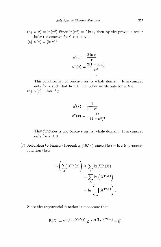
Solutions to Chapter Exercises 257
(b) u(x) = ln(x2) Since ln(x2) = 2 lnx, then by the previous result ln(x2) is concave for 0 < x < oo.
(c) u{x) = (lnx)2
. . . 2 lnx u (x)
u"(x)
x 2(1 - l n x )
This function is not concave on its whole domain. It is concave only for x such that lnx > 1, in other words only for x > e.
(d) u(x) = t a n - 1 x
u'{x) 1
1 + x2
u (x) = (1 + x2)2
This function is not concave on its whole domain. It is concave only for x > 0.
(7) According to Jensen's inequality (10.14), since f(x) = lnx is a concave function then
l n ( ^ X P ( x ) ) > J > X P ( X ) V x J x
= ] T l n ( x p W ) x
= ln(llxPm)-
Since the exponential function is monotone then
E [X] = e l n & * xp^) > e l n(n* *P<X)) = Q.
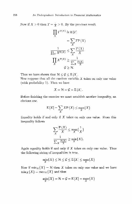
258 An Undergraduate Introduction to Financial Mathematics
Now if X > 0 then T = ^ > 0. By the previous result
l[T^xUeE[T] x
= ETPPO
<
X
£ P ( X )
Ylxxnx) - ^ x
x l^x x Q>n.
Thus we have shown that TL < Q < E [X]. Now suppose that all the random variable X takes on only one value (with probability 1). Then we have
X = H = Q = E [X].
Before finishing the exercise we must establish another inequality, an obvious one.
E[X] = ^ I P ( I ) < m f { I }
x
Equality holds if and only if X takes on only one value. From this inequality follows
Y ^ r 1 < m a x { - } ^ X x lX3
> min{X}. V M l " x 2-^x x
Again equality holds if and only if X takes on only one value. Thus the following string of inequalities is true.
min{X} < H < G < E [X] < max{X} yC -A
Now if m i n x { ^ } = 'H then X takes on only one value and we have mm.x{X} = m a x x { I } and thus
min{X} = H = Q = E [X] = max{X} X -A
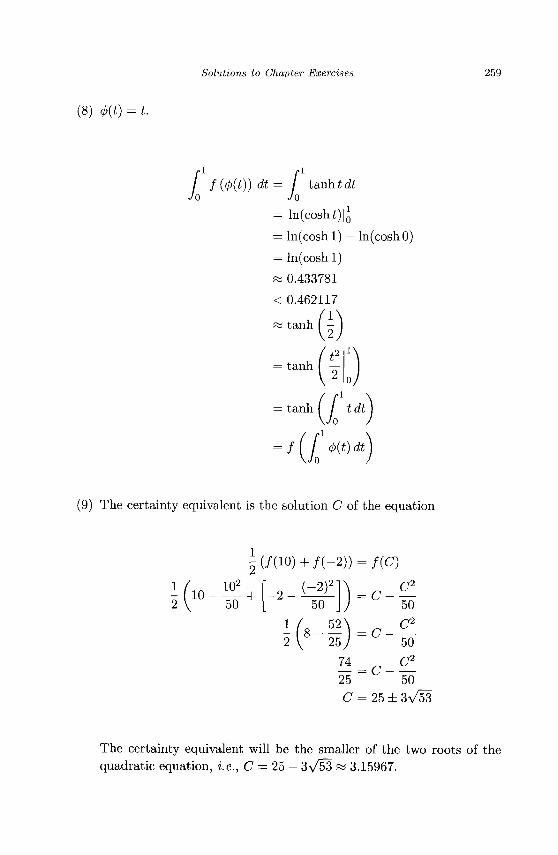
Solutions to Chapter Exercises 259
(8) <j>{t) = t.
f JO
f(<p(t)) dt= I t&nb.tdt Jo
= ln(cosh£)|0
= ln(coshl) - ln(coshO)
= ln(coshl)
« 0.433781
< 0.462117
tanh
tanh
tanh
/ % ( * ) Jo
dt
(9) The certainty equivalent is the solution C of the equation
2(/(10) + / ( " 2 ) ) = / (C)
102
-I 1 0 - — + 2 V 50
(~2)2
50
52 25
r2
= c- — 50 r2
= c- — 50
C2
25 50
C = 25 ± 3V53
The certainty equivalent will be the smaller of the two roots of the quadratic equation, i.e., C — 25 - 3\/53 w 3.15967.
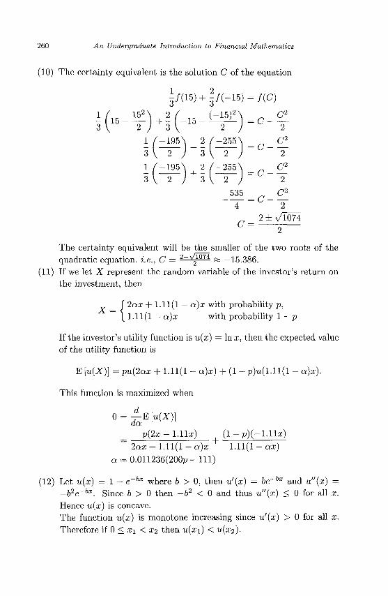
260 An Undergraduate Introduction to Financial Mathematics
(10) The certainty equivalent is the solution C of the equation
5/(15) + | / ( - 1 5 ) = / (C)
3 \ 2 J 3\ 2 ) 2
1 / - 1 9 5 \ . 2 / - 2 5 5 \ C2
Q — - -3 \ 2 / 3 \ 2 j 2 1 / - 1 9 5 \ 2 / - 2 5 5 \ C2
3 V 2 7 3 V 2 y 2 535 _ C2
2±V1074 C " 2
The certainty equivalent will be the smaller of the two roots of the quadratic equation, i.e., C = 2~v
21074 « —15.386.
(11) If we let X represent the random variable of the investor's return on the investment, then
J 2ax + 1.11(1 — a)x with probability p, \ 1.11(1 — a)x with probability 1 — p
If the investor's utility function is u(x) — \nx, then the expected value of the utility function is
E [u(X)\ = pu(2ax + 1.11(1 - a)x) + (1 - p )u( l . l l ( l - a)x).
This function is maximized when
o = A E [ t t W ]
p(2z - l . l l z ) ( l - p ) ( - l . l l a ; )
2ax + 1.11(1 -a)x 1.11(1 - ax)
a = 0.011236(200p-lll)
(12) Let u{x) = 1 - e~bx where 6 > 0, then u'{x) = be"hx and u"{x) = -b2e~bx. Since 6 > 0 then -b2 < 0 and thus u"(x) < 0 for all x. Hence u(x) is concave. The function u(x) is monotone increasing since u'(x) > 0 for all x. Therefore if 0 < x\ < Xi then u{xi) < u(x2)-
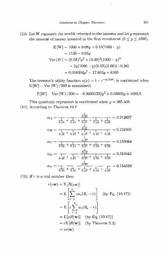
Solutions to Chapter Exercises 261
(13) Let W represent the wealth returned to the investor and let y represent the amount of money invested in the first investment (0 < y < 1000).
E [W] = 1000 + 0.0% + 0.13(1000 - y)
= 1130-0.05y
Var(W) = (0.03) V + (0.09)2(1000 - y)2
+ 2y(1000 - j/)(0.03)(0.09)(-0.26)
= 0.010404y2 - 17.604y + 8100
The investor's utility function u(x) = 1 — e~x /1 0 0 , is maximized when E [W] - Var (W) /200 is maximized.
E [W] - Var (W) /200 = -0.00005202y2 + 0.03802y + 1089.5
This quadratic expression is maximized when y « 365.436. (14) According to Theorem 10.7
a A = l
0.24
aB
cue
0.24 ~ 0.41 ~ 0.27 ~ 0.16 ' 0.33 1
0A1
0.24 ~ 0.41 ~ 0.27 ~ 0.16 ' 0.33 1
0.27
0.24 ~ 0.41 ~ 0.27 ^ 0.16 ' 1
0.16
1 0.33
aD = i 1
OLE
_1 | 1 . 1_ 0.24 "•" 0.41 """ 0.27 "• 0.16 ~r 0.33
1 0JS3
0.24 ~ 0.41 ~ 0.27 ' 0.16 ' 0.33
= 0.212697
= 0.124505
= 0.189064
= 0.319045
= 0.154689
(15) If c is a real number then
r(cw) = E [R(cw)
:E ^2cu>i(Ri -r) i=l
(by Eq. (10.17))
= E cy^jjJi(Ri - r )
= E[cR(w)] (by Eq. (10.17))
= cE [-R(w)] (by Theorem 2.3)
= cr(w).
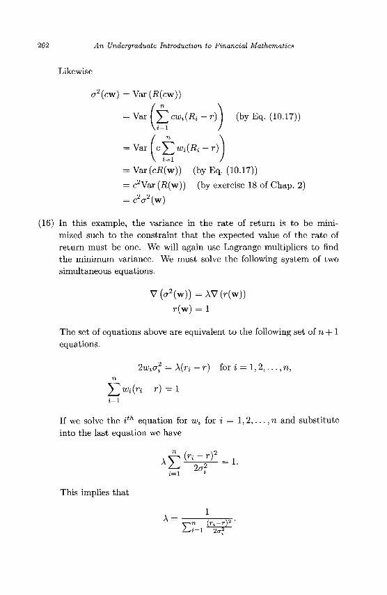
262 An Undergraduate Introduction to Financial Mathematics
Likewise
CT2(cw) = Var(i?(cw))
= Var [Y^cwiiRi - r) ] (by Eq. (10.17)) v i = l
Var Ic^MRi-r) \ t = i /
= Var (cR(w)) (by Eq. (10.17))
= c2Var (R(w)) (by exercise 18 of Chap. 2)
= c V ( w )
(16) In this example, the variance in the rate of return is to be minimized such to the constraint that the expected value of the rate of return must be one. We will again use Lagrange multipliers to find the minimum variance. We must solve the following system of two simultaneous equations.
V(cr2(w)) =AV(r(w))
r(w) = 1
The set of equations above are equivalent to the following set of n + 1 equations.
2wi(if = \{ri — r) for i = 1, 2 , . . . , n, n
Ywi(ri ~r) = l 1 = 1
If we solve the ith equation for Wi for i = 1,2,... ,n and substitute into the last equation we have
(ri - r)
1 = 1
This implies that
E n {ri—r)2
i=l 2a'2
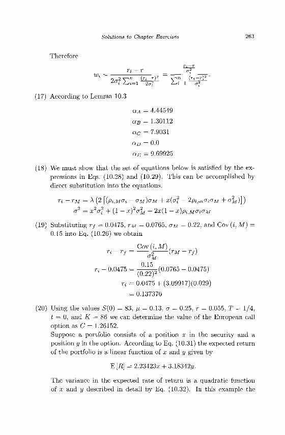
Solutions to Chapter Exercises 263
Therefore
2 v-^" (rj-r)2 ^ r a (ji_ 9 .2 V^« (n-r j" v^n z o i 2^=1 2o-2 Zw=l
(17) According to Lemma 10.3
2oT
aA = 4.44549
a B = 1.30112
ac = 7.9031
a D = 0.0
aE = 9.69925
(18) We must show that the set of equations below is satisfied by the expressions in Eqs. (10.28) and (10.29). This can be accomplished by direct substitution into the equations.
n - rM = A (2 [{pt^MCfi - a-M)(TM + x(cr2 - 2piimo-io-M + c^ ) ] )
a2 = x2a2 + (1 - x)2a2M + 2x(l - x)piMOiOM
(19) Substituting rf = 0.0475, rM = 0.0765, aM = 0.22, and Cav(i,M) = 0.15 into Eq. (10.26) we obtain
Cov (i, M) . n-rf = -J ( rM - rf)
"M
n - 0.0475 = 7 ^ 5 ( 0 - 0 7 6 5 - 0.0475)
n = 0.0475 + (3.09917)(0.029)
= 0.137376
(20) Using the values 5(0) = 83, \i = 0.13, a = 0.25, r = 0.055, T = 1/4, t = 0, and K = 86 we can determine the value of the European call option as C = 1.26152. Suppose a portfolio consists of a position x in the security and a position y in the option. According to Eq. (10.31) the expected return of the portfolio is a linear function of x and y given by
E [R] = 2.23423s + 3.18342y.
The variance in the expected rate of return is a quadratic function of x and y described in detail by Eq. (10.32). In this example the
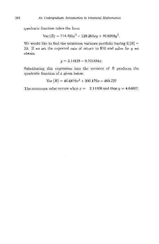
264 An Undergraduate Introduction to Financial Mathematics
quadratic function takes the form
Var (R) = 114.405a;2 + 129.264xy + 46.6908y2.
We would like to find the minimum variance portfolio having E [R] = 10. If we set the expected rate of return to $10 and solve for y we obtain
y = 3.14128 -0.701834a;.
Substituting this expression into the variance of R produces the quadratic function of x given below.
Var (R) = 46.6819a;2 + 200.179a; + 460.727
The minimum value occurs when x = —2.14408 and thus y = 4.64607.
Bibliography
Bleecker, D. and Csordas, G. (1996). Basic Partial Differential Equations, International Press, Cambridge, Massachusetts, USA.
Boyce, W. E. and DiPrima, R. C. (2001). Elementary Differential Equations and Boundary Value Problems, 7th edition, John Wiley and Sons, Inc., New York, USA.
Burden, R. L. and Faires, J. D. (2005). Numerical Analysis, 8th edition, Thomson Brooks/Cole, Belmont, CA, USA.
Churchill, R. V., Brown, J. W. and Verhey, R. F. (1976). Complex Variables and Applications, 3rd edition, McGraw-Hill Book Company, New York, USA.
Courant, R. and Robbins, H. (1969). What is Mathematics?, Oxford University Press, Oxford, UK.
Dean, J., Corvin, J. and Ewell, D. (2001). List of Playboy's playmates of the month with data sheet stats, Available at http://www3.sympatico.ca/jimdean/pmstats.txt.
DeGroot, M. H. (1975). Probability and Statistics, Behavioral Science: Quantitative Methods. Addison-Wesley Publishing Company, Reading, Massachusetts, USA.
Durrett, R. (1996). Stochastic Calculus: A Practical Introduction, CRC Press, Boca Raton, FL, USA.
Gale, D., Kuhn, H. W. and Tucker, A. W. (1951). Linear programming and the theory of games, in T.C. Koopmans, editor, Activity Analysis of Production and Allocation, Wiley, New York, NY, USA, pp. 317-329.
Gardner, M. (October 1959). "Mathematical Games" column, Scientific American, pp. 180-182.
Goldstein, L. J., Lay, D. C. and Schneider, D. I. (1999). Brief Calculus and Its Applications, 8th edition, Prentice Hall, Upper Saddle River, NJ, USA.
Golub, G. H. and Van Loan, C. F. (1989). Matrix Computations, 2nd edition, Johns Hopkins University Press, Baltimore, Maryland, USA.
Greenberg, M. D. (1998). Advanced Engineering Mathematics, 2nd edition, Prentice-Hall, Inc., Upper Saddle River, New Jersey, USA.
Jeffrey, A. (2002). Advanced Engineering Mathematics, Harcourt Academic Press, Burlington, Massachusetts, USA.
265
266 An Undergraduate Introduction to Financial Mathematics
Kijima, M. (2003). Stochastic Processes with Applications to Finance, Chapman & Hall/CRC, Boca Raton, FL, USA.
Luenberger, D. G. (1998). Investment Science, Oxford University Press, New York, USA.
Marsden, J. E. and Hoffman, M. J. (1987). Basic Complex Analysis, W. H. Freeman and Company, New York, NY, USA.
Mikosch, T. (1998). Elementary Stochastic Calculus With Finance in View, Vol. 6 of Advanced Series on Statistical Science & Applied Probability, World Scientific Publishing, River Edge, New Jersey, USA.
Neftci, S. N. (2000). An Introduction to the Mathematics of Financial Derivatives, 2nd edition, Academic Press, San Diego, CA, USA.
Redner, S. (2001). A Guide to First Passage Processes, Cambridge University Press, Cambridge, UK.
Ross, S. M. (1999). An Introduction to Mathematical Finance: Options and Other Topics, Cambridge University Press, Cambridge, UK.
Ross, S. M. (2006). A First Course in Probability, 7th edition, Prentice Hall, Inc., Upper Saddle River, NJ, USA.
Selvin, S. (1975). A problem in probability, American Statistician, 29, 1, p. 67. Smith, R. T. and Minton, R. B. (2002). Calculus, 2nd edition, McGraw-Hill,
Boston, MA, USA. Steele, J. M. (2001). Stochastic Calculus and Financial Applications, Volume 45
in Applications of Mathematics, Springer-Verlag, New York, NY, USA. Stewart, J. (1999). Calculus, 4th edition, Brooks/Cole Publishing Company, Pa
cific Grove, CA, USA. Strang, G. (1986). Introduction to Applied Mathematics, Wellesley-Cambridge
Press, Wellesley, MA, USA. Taylor, A. E. and Mann, W. R. (1983). Advanced Calculus, 3rd edition, John
Wiley & Sons, Inc., New York, NY, USA. vos Savant, M. (February 1990). "Ask Marilyn" column, Parade Magazine, p. 12. Wilmott, P., Howison, S. and Dewynne, J. (1995). The Mathematics of Financial
Derivatives: A Student Introduction, Cambridge University Press, Cambridge, UK.
Index
absorbing boundary condition, 80, 113
Addition rule, 18 additivity, 40 American option, 103 annuity, 8 arbitrage, 63, 110 Arbitrage Theorem, 63, 72, 104 area as probability, 36 arithmetic mean, 192 augmented matrix, 87 average, see expected value
backwards parabolic equation, 112 backwards substitution, 87, 89 bell curve, 42 Bernoulli random variable, 23, 79 beta, 184 betting strategy, 72 binary model, 107 binomial model, 115 binomial random variable, 23, 42 Black-Scholes equation, 104, 110 boundary condition, 89, 112
absorbing, 80 European call option, 113
Brownian motion, 187
call option, 103 Capital Asset Pricing Model, 183 capital market line, 182, 184
CAPM, see Capital Asset Pricing Model
centered difference formula, 45 Central Limit Theorem, 49, 176 certainty equivalent, 172 chain rule, 98, 132
multivariable, 99 closing price, 95 compound amount, 2 compound interest, 3 compounding period, 3 concavity, 135, 167 conditional exit time, 90 conditional probability, 19 constrained optimization, 179 constraints, 65
equality, 65 inequality, 65
continuous distribution, 36 continuous probability, 36 continuous random variable, 35 continuous random walk, 91 continuous stochastic process, 93 continuously compounded interest, 5 convex set, 65 correlation, 155, 159 cost function, 65 covariance, 155 cumulative distribution function, 48
Delta, 133, 145 Delta neutrality, 145, 150
267
268 An Undergraduate Introduction to Financial Mathematics
dependent random variables, 40 derivative, 131
financial, 110 deterministic process, 92 deviation, 41 difference equation, 84 differential equation
stochastic, 94, 96 differentiation
chain rule, 98 discrete outcome, 16 distribution
continuous, 36 distribution function, 36 drift, 51, 163, 187 dual, 67 Duality Theorem, 65, 71
effective interest rate, 3 efficient markets, 63 equality constraints, 65 Euler Identity, 116 European call option
boundary condition, 113 European option, 103
call flnal condition, 112
event, 15 certain, 16 discrete, 15 impossible, 16
events compound, 17 independent, 21 mutually exclusive, 17
excess rate of return, 184 exercise time, 103 exit time, 90 expected rate of return, 180 expected utility, 171 expected value, 15, 24, 38
of normal random variable, 47 experiment, 15 expiry date, 103 exponential decay, 123 exponential growth, 5, 91
Extreme Value Theorem, 178
feasible vector, 65 final condition, 111
European call option, 112 financial derivative, 110 finite differences, 45 Fourier Convolution, 117 Fourier Transform, 115
alternative definition, 119 definition, 115 existence, 116 of a convolution, 118 of a derivative, 117
frequency, 116 function
concave, 167 utility, 166
Fundamental Theorem of Calculus, 132
future value, 5
Gamma, 135, 148, 151 Gamma neutrality, 151 Gaussian elimination, 87 generalized Wiener process, 97 geometric mean, 192 geometric series, 7 gradient operator, 179 Greeks, 131
harmonic mean, 192 heat equation, 111, 120 hedge and forget, 146 hedging, 136, 143, 164 hockey stick, 112
in the money, 112, 153 independent events, 21 independent random variables, 40 inequality constraints, 65 inflation, 10
rate of, 10 initial condition, 111 interest, 1
compound, 3
Index 269
continuously compounded, 5 effective rate, 3 simple, 2
interest rate, 1 Inverse Fourier Transform, 119 investor
risk-averse, 168 risk-neutral, 168
Ito process, 97 Ito's Lemma, 100, 110, 187
Jensen's Inequality, 170, 171 Continuous Version, 171 Discrete Version, 170
joint probability function, 26, 39
Lagrange Multipliers, 179, 185 Laplacian equation, 84 linear programming, 65 linear systems
tridiagonal, 87 linearity, 140 loans, 7 lognormal random variable, 51, 163,
188 long position, 104, 187
marginal distribution, 40 marginal probability, 27 matrix
upper triangular, 87 mean, see expected value, see
expected value Mean Value Theorem, 169 minimum variance, 163, 165, 177 Monty Hall problem, 18 Multiplication rule, 20
noise, 92 normal probability distribution, 42,
48 normal random variable, 35, 42
odds, 64 operations research, 65 optimal portfolio, 164
option, 103 American, 103 call, 103 European, 103 put, 103
option pricing formula European call, 125 European put, 125
out of the money, 112, 153 outcome, 15
discrete, 15, 16
partial differential equation, 111 Black-Scholes, 104, 139 linear, 111 parabolic type, 111 second order, 111
PDE, see partial differential equation Poisson equation, 86 polar coordinates, 46 portfolio, 140, 162
Delta-neutral, 145 Gamma neutral, 151 optimal, 164 rebalancing, 146
portfolio selection problem, 173, 175 Portfolio Separation Theorem, 180 position
long, 104 short, 104
positive part, 55 present value, 1, 5, 110 pricing formula
European call option, 125 European put option, 125
primal, 67 principal, see principal amount principal amount, 2 probability, 16
classical, 16 conditional, 19 continuous, 36 empirical, 16 marginal, 27
probability distribution, 21 normal, 48
270 An Undergraduate Introduction to Financial Mathematics
probability distribution function, 36 put option, 103 Put-Call Parity, 106 Put-Call Parity Formula, 134
random experiment, 166 random variable, 15
Bernoulli, 79 binomial, 15, 42 continuous, 35 discrete, 15 lognormal, 51, 163 normal, 35, 42 uncorrelated, 159, 178 uniform, 37
random walk, 77 continuous, 91
rate of inflation, 10 rate of return, 1, 11, 155, 162
excess, 184 expected value, 180 variance, 180
rebalancing, 146 retirement, 8 return
rate of, see rate of return, 11 Rho, 138 risk, 185 risk-averse investor, 168 risk-neutral investor, 168
samples means, 49 Schwarz Inequality, 160 secant lines, 168 sensitivity, 131 separation of variables, 111, 123 short position, 104, 187 simple interest, 2 slack variables, 65 spatial homogeneity, 82
spread, see standard deviation standard deviation, 15, 32, 41 standard normal random variable, 48 Stirling's formula, 44 stochastic calculus, 77 stochastic differential equation, 94, 96 stochastic process, 92, 96
continuous, 93 stochastic processes, 110 stopping time, 83 strike price, 103 strike time, 103 surrogate, 164 symmetric random walk, 78
Taylor remainder, 99 Taylor series, 150 Taylor's Theorem, 98 Theta, 131 Treasury Bonds, 105 tridiagonal linear systems, 87 tridiagonal matrix, 87
uncorrelated random variable, 159 uniform random variable, 37 upper triangular matrix, 87 utility, 166
decreasing, 167 utility function, 166, 167
variance, 29, 41 alternative formula, 41 minimum, 163 of normal random variable, 47
vector inequalities, 66 Vega, 136 volatility, 51, 92, 96, 137, 163, 187
Weak Duality Theorem, 68 Wiener process, 97, 187
A n U n d e r g r a d u a t e
I n t r o d u c t i o n t o
F i n a n c i a l --w M a t h e m a t i c s
This textbook provides an introduction
to financial mathematics and financial
engineering for undergraduate
students who have completed a three or
four semester sequence of calculus courses.
It introduces the theory of interest, random
variables and probability, stochastic processes,
arbi t rage, option pr ic ing, hedging, and
portfolio optimization.The student progresses
from knowing only elementary calculus to
understanding the derivation and solution of
the Black-Scholes partial differential equation
and its solutions. This is one of the few books
on the subject of financial mathematics which
is accessible to undergraduates having only a
thorough grounding in elementary calculus.
It explains the subject matter without "hand
waving" arguments and includes numerous
examples. Every chapter concludes with a set
of exercises which test the chapter's concepts
and fill in details of derivations.
6009 he ISBN 981 256-637-6
orld Scientific YEARS OF PUBLISHING
3 1 - 2 o o 6 www.worldscientific.com