an optimal control strategy to determine diffusivity...
TRANSCRIPT
AN OPTIMAL CONTROL STRATEGY TO DETERMINE DIFFUSIVITY
VERSUS CONCENTRATION IN TERNARY SYSTEMS OF TWO GASES
AND A NON VOLATILE PHASE
By
Amir Jalal Sani
M.Sc in Applied Chemistry, University of Karachi, Karachi, 1993
M.A.Sc in Chemical Engineering, Ryerson University, Toronto, 2010
A dissertation presented to
Ryerson University
In the partial fulfillment of the Requirements for the degree of
Doctor of Philosophy
In the program of
Chemical Engineering
Toronto, Ontario, Canada, 2014
© Amir Jalal Sani 2014

ii
Author’s Declaration
I here declare that I am the sole author of this dissertation. This is a true copy of the
dissertation, including any required final revisions, as accepted by my examiners.
I authorize Ryerson University to lend this dissertation to other institutions or individuals
for the purpose of scholarly research.
I further authorize Ryerson University to reproduce this dissertation by photocopying or by
other means, in total or in part, at the request of other institutions or individuals for the
purpose of scholarly research.
iii
AN OPTIMAL CONTROL FRAMEWORK TO DETERMINE DIFFUSIVITY VERSUS CONCENTRATION SURFACES IN TERNARY SYSTEMS OF
TWO GASES AND A NON VOLATILE PHASE Doctor of Philosophy
2014 Amir Jalal Sani
Chemical Engineering Ryerson University
Abstract
Diffusivity is a strong function of concentration and an important transport property.
Diffusion of multiple species is far more frequent than the diffusion of one species.
However, there are limited experimental data available on multi-component diffusivity.
The objective of this study is to develop an optimal control framework to determine multi-
component, concentration-dependent diffusivities of two gases in a non-volatile phase
such as polymer.
In Part 1 of this study, we derived a detailed mass-transfer model of the experimental
diffusion process for the non-volatile phase to provide the temporal masses of gases in the
polymer. The determination of diffusivities is an inverse problem involving principles of
optimal control. Necessary conditions are determined to solve this problem.
In Part 2 of this study, we utilized the results of Part 1 to determine the concentration-
dependent, multi-component diffusivities of nitrogen and carbon dioxide in polystyrene. To

iv
that end, solubility and diffusion experiments are conducted to obtain necessary data. In
the ternary system of nitrogen (1), carbon dioxide (2), and polystyrene (3), the diffusivities
and versus the gas mass fractions are two-dimensional surfaces.
The diffusivity of carbon dioxide was found to be greater than that of nitrogen. The value of
the main diffusion coefficient was found to increase as the concentration of carbon
dioxide increased. The highest value of obtained was for nitrogen
mass fraction of and for a carbon dioxide mass fraction of . The
cross-diffusion coefficient increased as the concentrations of nitrogen and carbon
dioxide increased. The diffusivity reached its maximum value when the concentrations of
nitrogen and carbon dioxide were at their maximum values. The diffusivity was of the order
of .
The diffusivity of the cross-diffusion coefficient was found to be increased for the mass
fractions of carbon dioxide ranging from 0 to . The diffusivity was found to be
of the order of . The diffusion coefficient, was found to increase with the
concentrations of nitrogen and carbon dioxide, remained high with low concentrations
of carbon dioxide. The diffusivity was found to be of the order of .
v
Acknowledgement
I take this opportunity to express my profound gratitude and deep regards to my guide
Professor Dr. Simant R. Upreti for his exemplary guidance, monitoring and constant
encouragement throughout the course of this thesis. The blessing, help and guidance given
by him time to time shall carry me a long way in the journey of life on which I am about to
embark.
I also take this opportunity to express a deep sense of gratitude to Professor Dr. Farhad
Ein-Mozaffari and Professor Dr. Jiangning Wu for their cordial support, valuable
information and guidance, which helped me in completing this task through various stages.
I am obliged to engineering specialists Ali Hemmati, Daniel Boothe, Tondar Tajrobehkar,
and technical specialist Shawn McFadden, for the valuable information provided by them in
their respective fields. I am grateful for their cooperation during the period of my
assignment.
My completion of this project could not have been accomplished without the support of
my children, thank you for allowing me time away from you to research and write. To my
caring, loving, and supportive wife, Yasmin: my deepest gratitude. Your encouragement
when the times got rough are much appreciated and duly noted.
Lastly, I thank almighty without which this assignment would not be possible.
Amir Sani
vi
Dedication
I dedicate this work to my spiritual mentors
Khwaja Shamsuddin Azeemi
and
Master Choa Kok Sui

vii
Table of Content
Author’s Declaration ........................................................................................................................ii
Abstract ........................................................................................................................................... iii
Acknowledgement ........................................................................................................................... v
Dedication ....................................................................................................................................... vi
Table of Content ............................................................................................................................ vii
List of Tables ................................................................................................................................... ix
List of Figures ................................................................................................................................... x
NOMENCLATURE ............................................................................................................................ xii
1 INTRODUCTION ....................................................................................................................... 2
1.1 Definition of Multi-component Diffusion ........................................................................ 6
1.1.1 The Origin of Fick’s Law ............................................................................................ 7
1.1.2 Diffusion in Gases...................................................................................................... 7
1.1.3 Diffusion in Liquids .................................................................................................... 9
1.1.4 Fick’s Law ................................................................................................................ 11
1.2 Structure of the Thesis ................................................................................................... 15
2 LITERATURE REVIEW .............................................................................................................. 17
2.1 Lack of Data for Ternary System .................................................................................... 20
2.2 Optimal Control .............................................................................................................. 23
3 EXPERIMENTAL SETUP ........................................................................................................... 28
3.1 Solubility Experiments .................................................................................................... 36
3.2 Diffusion Experiments .................................................................................................... 37
3.3 Analysis of Gas Phase Composition................................................................................ 38
3.3.1 Gas Chromatography .............................................................................................. 38
3.3.2 Chromatogram ........................................................................................................ 39
3.3.3 Sampling .................................................................................................................. 40
4 THEORY and COMPUTATION ................................................................................................. 42
4.1 Mass Transfer Model ..................................................................................................... 42

viii
4.2 Theoretical Model Development ................................................................................... 45
4.3 Optimal Control .............................................................................................................. 51
4.4 The Objective Functional................................................................................................ 52
4.5 Necessary Condition for the Minimum .......................................................................... 54
4.6 Computational Algorithm ............................................................................................... 77
5 RESULTS and DISCUSSION ..................................................................................................... 83
5.1 Diffusivity Correlations ................................................................................................... 99
5.2 Sensitivity Analysis ......................................................................................................... 99
6 CONCLUSIONS and RECOMMENDATIONS ........................................................................... 102
6.1 CONCLUSIONS .............................................................................................................. 102
6.2 RECOMMENDATIONS ................................................................................................... 104
References .................................................................................................................................. 105
Appendix A .................................................................................................................................. 109
Appendix B .................................................................................................................................. 112
Appendix C .................................................................................................................................. 116
Appendix D .................................................................................................................................. 135
ix
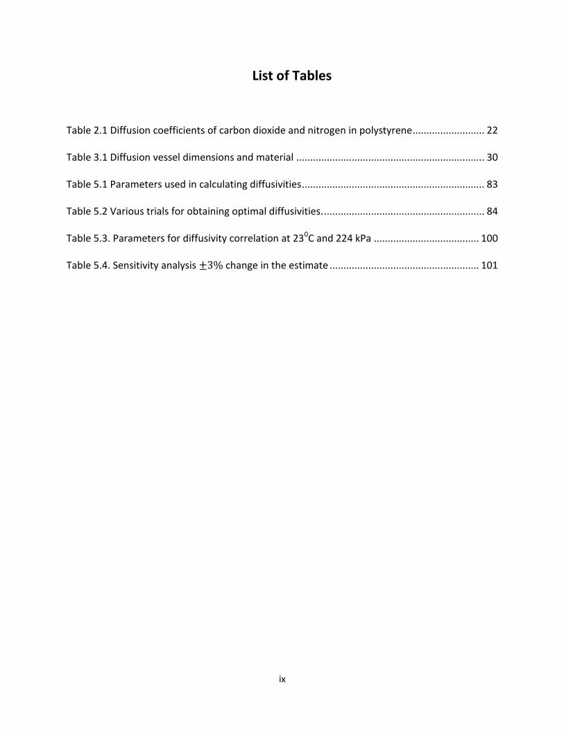
List of Tables
Table 2.1 Diffusion coefficients of carbon dioxide and nitrogen in polystyrene.......................... 22
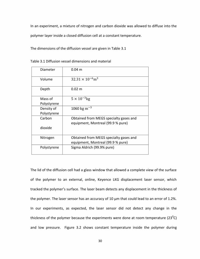
Table 3.1 Diffusion vessel dimensions and material .................................................................... 30
Table 5.1 Parameters used in calculating diffusivities .................................................................. 83
Table 5.2 Various trials for obtaining optimal diffusivities. .......................................................... 84
Table 5.3. Parameters for diffusivity correlation at 230C and 224 kPa ...................................... 100
Table 5.4. Sensitivity analysis change in the estimate ...................................................... 101

x
List of Figures
Figure 1.1. Two homogeneous mixtures separated by a polymer membrane .............................. 3
Figure 1.2. Equimolar mixture of hydrogen and argon in Tube 1; equimolar mixture of methane
and argon in Tube 2. ....................................................................................................................... 5
Figure 1.3. Nickel ions diffusing from an acidic solution through a membrane into a strong acid 6
Figure 1.4. Graham’s apparatus for the study of diffusion ............................................................ 8
Figure 1.5. (a) Diffusion in bottles with salt solution; (b) empty bottle in a jar that contains only
water ............................................................................................................................................. 10
Figure 1.6. Multi-component diffusion in nitrogen, carbon dioxide, and polystyrene ................ 13
Figure 3.1. Experimental setup ..................................................................................................... 29
Figure 3.2 Polymer temperature during diffusion experiment .................................................... 31
Figure 3.3 Polymer thickness during diffusion experiments ........................................................ 32
Figure 3.4. (a) Laser sensor; (b) thermocouple ............................................................................. 33
Figure 3.5. Polystyrene layer with uniform thickness .................................................................. 35
Figure 3.6. Magnetic mixer ........................................................................................................... 36
Figure 4.1. Diffusion of two gases in an underlying dense, non-volatile phase ........................... 44
Figure 4.2. Methodology for determining diffusivities ................................................................. 80
Figure 4.3 Architecture of the computer program ....................................................................... 81
Figure 5.1 Convergence of objective functional ........................................................................... 89
Figure 5.2 Experimental and calculated mass of carbon dioxide absorbed in polystyrene. ........ 90
Figure 5.3. Experimental and calculated mass of nitrogen absorbed in polystyrene .................. 90
xi
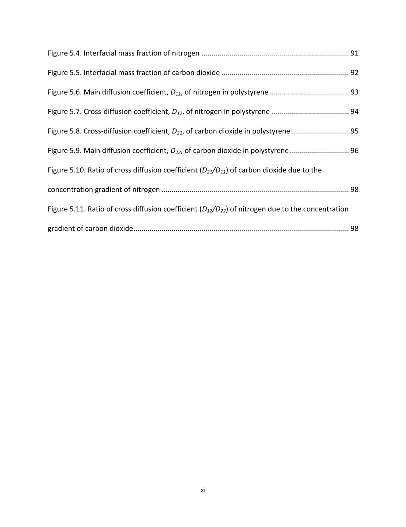
Figure 5.4. Interfacial mass fraction of nitrogen .......................................................................... 91
Figure 5.5. Interfacial mass fraction of carbon dioxide ................................................................ 92
Figure 5.6. Main diffusion coefficient, D11, of nitrogen in polystyrene ........................................ 93
Figure 5.7. Cross-diffusion coefficient, D12, of nitrogen in polystyrene ....................................... 94
Figure 5.8. Cross-diffusion coefficient, D21, of carbon dioxide in polystyrene ............................. 95
Figure 5.9. Main diffusion coefficient, D22, of carbon dioxide in polystyrene .............................. 96
Figure 5.10. Ratio of cross diffusion coefficient (D21/D11) of carbon dioxide due to the
concentration gradient of nitrogen .............................................................................................. 98
Figure 5.11. Ratio of cross diffusion coefficient (D12/D22) of nitrogen due to the concentration
gradient of carbon dioxide ............................................................................................................ 98
xii
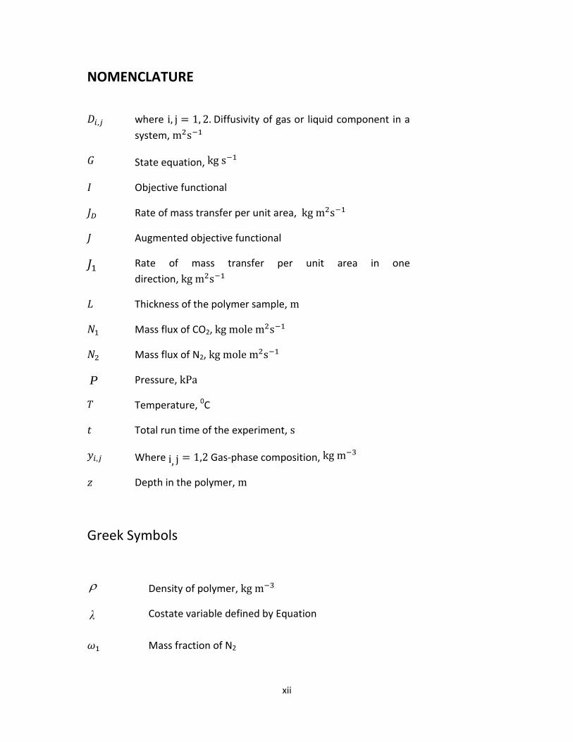
NOMENCLATURE
where Diffusivity of gas or liquid component in a
system,
State equation,
Objective functional
Rate of mass transfer per unit area,
Augmented objective functional
Rate of mass transfer per unit area in one
direction,
Thickness of the polymer sample,
Mass flux of CO2,
Mass flux of N2,
P Pressure,
Temperature, 0C
Total run time of the experiment,
Where Gas-phase composition,
Depth in the polymer,
Greek Symbols
Density of polymer,
λ Costate variable defined by Equation
Mass fraction of N2
xiii
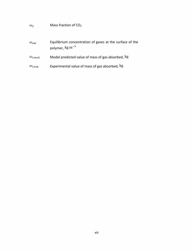
Mass fraction of CO2
Equilibrium concentration of gases at the surface of the
polymer,
Model predicted value of mass of gas absorbed,
Experimental value of mass of gas absorbed,

2
1 INTRODUCTION
Diffusion can be defined in very simple terms as the movement of molecules from one
place to another due to a concentration gradient (Philibert, 2005). Chemical engineers
frequently deal with situations in which three or more components move from one place to
another at the same time. The conventional approach of mass transfer in a system is based
on the assumption that the movement of a chemical species from one place to another is
directly proportional to a driving force. The problem is that this assumption is only good for
cases in which diffusion is occurring in a two-component system (binary system), in a
system in which one component is diluted by a large excess of one or more of the other
components, or in a system in which all of the components in the mixture have similar
quantities and natures.
The question arises concerning whether the three or more components diffusing in a
system can be dealt in a same way as the components of a binary system. Answer to this
question is “No,” so we must deal with the problem of how to deal with a multi-component
system. Concerns such as this have been on the minds of chemical engineers for a long
time(Krishnamurthy & Taylor, 1982).
Multi-component diffusion systems exhibit characteristics that are quite different from
those of binary systems. In addition, methods have been developed to predict multi-
component diffusion in a consistent way using matrix formulations (E. L. Cussler, 2009). The
3
matrix of a multi-component system can be incorporated into powerful computer
software, which can be used in equipment design. This is one practical application of the
multi-component diffusion matrix.
Multi-component diffusion occurs when the flux of one component is influenced by the
concentration gradient of a second component. For example, the flux of the first
component can be increased by as much as an order of magnitude by changing the
concentration gradient of the second component. In multicomponent diffusion, the first
component can diffuse against its concentration gradient, i.e., from a region of lower
concentration to the region of higher concentration. The following examples explain these
effects in detail.
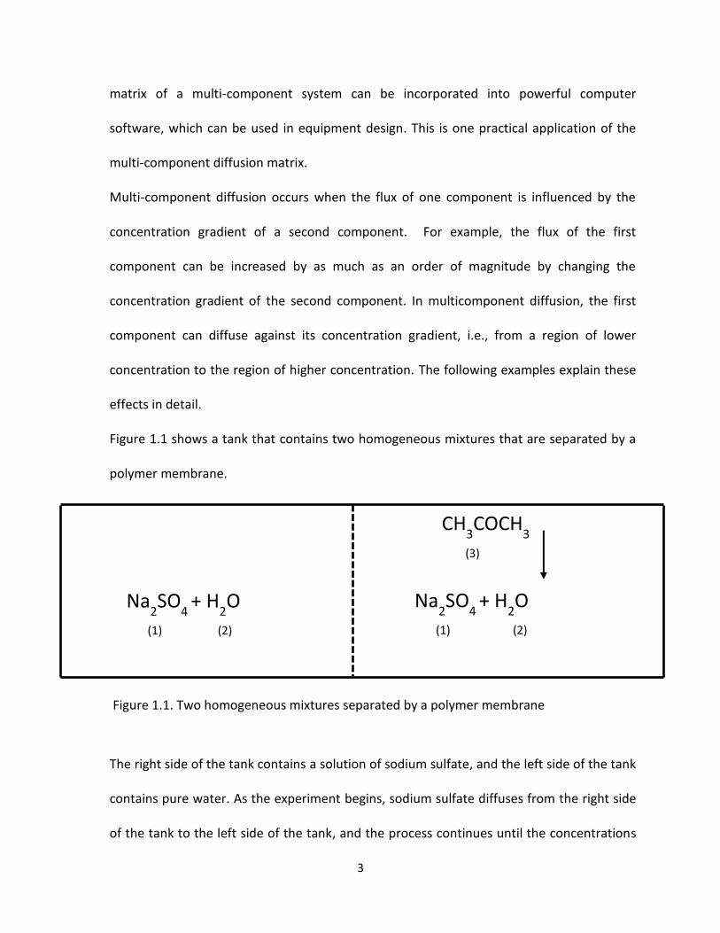
Figure 1.1 shows a tank that contains two homogeneous mixtures that are separated by a
polymer membrane.
Figure 1.1. Two homogeneous mixtures separated by a polymer membrane
The right side of the tank contains a solution of sodium sulfate, and the left side of the tank
contains pure water. As the experiment begins, sodium sulfate diffuses from the right side
of the tank to the left side of the tank, and the process continues until the concentrations
Na2SO
4 + H
2O
(1) (2)
CH3COCH
3
(3)
Na2SO
4 + H
2O
(1) (2)
4
of sodium sulfate are equal on both sides of the tank. At this point, if acetone is added to
the right side of the tank, the diffusion rate of sodium sulfate to the left side of the tank
increases. As more acetone is added, more sodium sulfate diffuses to the other side of the
membrane. However, if acetone is added to the left side of the tank, the rate of diffusion of
sodium sulfate is decreased, and, if acetone is added on both sides of the porous
membrane, the diffusion of sodium sulfate is increased slightly. This shows that the
gradient of acetone strongly influences the diffusion of sodium sulfate (E. L. Cussler &
Breuer, 1972).
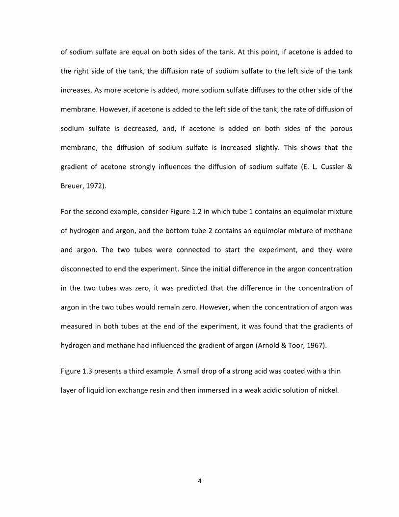
For the second example, consider Figure 1.2 in which tube 1 contains an equimolar mixture
of hydrogen and argon, and the bottom tube 2 contains an equimolar mixture of methane
and argon. The two tubes were connected to start the experiment, and they were
disconnected to end the experiment. Since the initial difference in the argon concentration
in the two tubes was zero, it was predicted that the difference in the concentration of
argon in the two tubes would remain zero. However, when the concentration of argon was
measured in both tubes at the end of the experiment, it was found that the gradients of
hydrogen and methane had influenced the gradient of argon (Arnold & Toor, 1967).
Figure 1.3 presents a third example. A small drop of a strong acid was coated with a thin
layer of liquid ion exchange resin and then immersed in a weak acidic solution of nickel.

5
Figure 1.2. Equimolar mixture of hydrogen and argon in Tube 1; equimolar mixture of methane and argon in Tube 2.
At the beginning of the experiment, the nickel diffused from the outside of the drop into
the drop across a membrane. But the diffusion of the nickel did not stop even when the
concentration of nickel was the same on both sides of the membrane. Nickel continued to
diffuse into the drop even when the concentration of nickel inside the drop was many
times greater than the concentration outside the drop. In this example, the concentration
difference of the acid causes a flux of nickel against its gradient. Above three examples
shows multi-component diffusion in which the flux of one solute is a function of the
gradient of the second solute.
Tube 1
Equimolar mixture
of H2 and Ar
Equimolar mixture
of CH4 and Ar
Tube 2

6
Figure 1.3. Nickel ions diffusing from an acidic solution through a membrane into a strong acid
1.1 Definition of Multi-component Diffusion
To understand multi-component diffusion, first, we need to discuss binary diffusion briefly
because it forms the basis for the multi-component diffusion that is discussed in the rest of
this thesis. We begin with Fick’s law, which describes the basic relationships in binary
diffusion. The diffusion coefficient described by this law is discussed for gases and liquids.
Diffusion in solids is not covered because it is not relevant, so, after discussing gases and
liquids, the structure of the thesis is presented. Then, multi-component diffusion is
addressed, including the optimal control framework for determining multi-component
diffusion
Thin layer of
liquid Ion
Exchange resin
Drop of strong acid
Weak acidic solution
of Ni++

7
1.1.1 The Origin of Fick’s Law
Early studies of diffusion were split into studies of gases and liquids. Researchers interested
in understanding the behaviors of atoms or molecules were focussed on studying gases.
Researchers working in the areas of medicine and physiology wanted to understand
biological transport processes, so they focused on the study of liquids, primarily the
diffusion of liquids across membranes (Fick, 1995). Let’s look briefly at the diffusion of
gases and liquids.
1.1.2 Diffusion in Gases
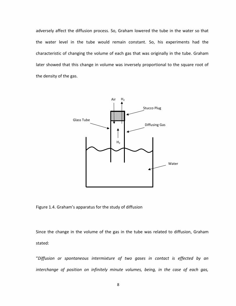
Thomas Graham (1829, 1833) was the first to analyze the diffusion process quantitatively.
Most of his research was conducted using the diffusion apparatus shown below in Figure
1.4. As shown in Figure 1.4, Graham’s apparatus consisted of a glass tube, one end of which
was immersed in water, with the other end closed by a stucco plug. The tube was filled
with hydrogen. Initially, the hydrogen diffuses out of the tube through the stucco plug,
while air diffuses into the tube from the outside.
The flux of hydrogen leaving the tube was not equal to the flux of air entering the tube, so
the level of the water in the tube rises during diffusion (Graham, 1833). Graham observed
that the rise in the water level in the tube would cause a pressure gradient that would
8
H2
Glass Tube
Stucco Plug
Diffusing Gas
Water
H2
Air
adversely affect the diffusion process. So, Graham lowered the tube in the water so that
the water level in the tube would remain constant. So, his experiments had the
characteristic of changing the volume of each gas that was originally in the tube. Graham
later showed that this change in volume was inversely proportional to the square root of
the density of the gas.
Figure 1.4. Graham’s apparatus for the study of diffusion
Since the change in the volume of the gas in the tube was related to diffusion, Graham
stated:
“Diffusion or spontaneous intermixture of two gases in contact is effected by an
interchange of position on infinitely minute volumes, being, in the case of each gas,
9
inversely proportional to the square root of the density of the gas…” (Graham, 1833). In
other words, ‘Diffusion is inversely proportional to the square root of the molecular weight
of the gas”.
Graham’s diffusion experiments did not say anything about the diffusion coefficient of the
gas. Since there was no pressure difference across the porous plug, the process of diffusion
across the porous plug could be easily explained without any need of Fick’s law or diffusion
coefficients (Masom & and Kronstadt, 1967). This is an example of an isobaric diffusion
process rather than the equimolar diffusion process that commonly is used to measure
diffusion coefficients. Graham’s experiments attracted attention towards diffusion as an
interesting molecular process, but he was unable to develop a basic diffusion law.
1.1.3 Diffusion in Liquids
The results of early experiments involving diffusion in liquids were difficult to interpret due
to the presence of the membrane in the diffusion process. Fick quoted Von Bruke (1843), a
physiologist who used olive oil and turpentine on the opposite sides of the leather
membrane and then he measured the change in the volume due to diffusion. This
experiment supported the hypothesis of the osmotic effect. But, the presence of the
membrane made the analysis of the diffusion process difficult.
10
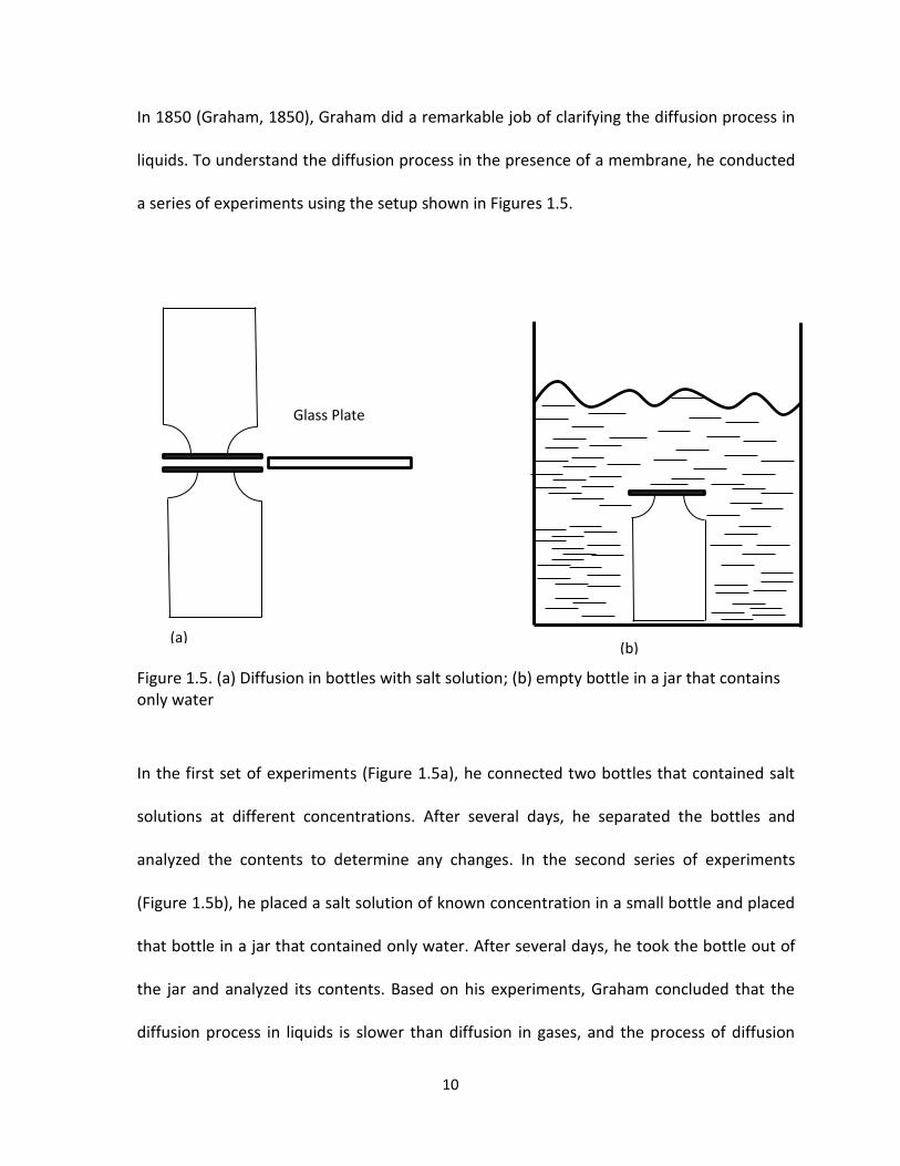
In 1850 (Graham, 1850), Graham did a remarkable job of clarifying the diffusion process in
liquids. To understand the diffusion process in the presence of a membrane, he conducted
a series of experiments using the setup shown in Figures 1.5.
Figure 1.5. (a) Diffusion in bottles with salt solution; (b) empty bottle in a jar that contains only water
In the first set of experiments (Figure 1.5a), he connected two bottles that contained salt
solutions at different concentrations. After several days, he separated the bottles and
analyzed the contents to determine any changes. In the second series of experiments
(Figure 1.5b), he placed a salt solution of known concentration in a small bottle and placed
that bottle in a jar that contained only water. After several days, he took the bottle out of
the jar and analyzed its contents. Based on his experiments, Graham concluded that the
diffusion process in liquids is slower than diffusion in gases, and the process of diffusion
Glass Plate
(a) (b)
11
becomes even slower as the diffusion progresses. After analyzing the results of his
experiments, Graham concluded that“ the quantities diffused appear to be closely in
proportion to the quantity of salt in the diffusion solution” (Graham, 1850). In other words,
“…the flux caused by diffusion is proportional to the concentration difference of the salt.”
1.1.4 Fick’s Law
In 1855, Fick put Graham’s experimental results on a quantitative basis. He described the
diffusion on the same mathematical basis as Fourier’s law of heat conduction or Ohm’s Law
for electrical conduction. Fick recognized more clearly that diffusion is a dynamic molecular
process than Graham did. With this basic hypothesis, Fick developed the laws of diffusion
using analogies with Fourier’s work. He described a one-dimensional flux, , by the
following equation:
(1.1)
where is the concentration, and is the distance. This is Fick’s law of diffusion. The
quantity , which Fick referred to as the “constant that depends on the nature of the
substance,” is also called the diffusion coefficient. Fick used Fourier’s development to
determine the more general conservation equation:
(
) (1.2)
where is the area and is a constant in a given system. So, Equation (1.2) becomes:
12
(
) (1.3)
Equation (1.3) is the basic equation for one-dimensional, unsteady state diffusion. Later,
Fick proved his hypothesis that diffusion and thermal conduction could be described by the
same equation.
Dense-phase molecular diffusivities are a complex process, and they can be a strong
function of composition, temperature, and pressure. Often, they are characterized by the
Fick diffusivity, which is a product of the Maxwell-Stefan diffusivity and a thermodynamic,
non-ideality factor that is related to the concentration of a chemical species in the medium
(E. L. Cussler, 2009). Fick diffusivity is a function of the concentration of the diffusing
substance at a given temperature and pressure. This non-ideality is notably present in
chemical systems at finite concentrations (Amooghina, et al., 2013; Bouchet et al., 1965;
Felder & Huvard, 1980; Ghoreyshi, et al., 2004; Liu, et al., 2011; Moradi Shehni, et al.,2011;
Rehfeldt & Stichlmair, 2007; Williams & Cady, 1934).
Multi-component diffusivities, i.e., the simultaneous diffusivities of two or more species in
a medium, are far more frequent than the diffusion of a single species (E. L. Cussler &
Peter, 1966).
Binary diffusion can be expressed mathematically as:
(1.4)
Equation (1.4) is another form of Fick’s first law of diffusion. The diffusion coefficient is
called binary diffusivity and is the total concentration. There is only one independent

13
driving force, , and one independent flux, . However, in a ternary mixture, there are
two independent fluxes and two independent driving forces Thus we
can write:
(1.5)
(1.6)
Equations (1.5) and (1.6) show that both fluxes depend on both of the independent
mole-fraction gradients The are the multi-component
diffusivities. These four diffusivity coefficients are needed to characterize a ternary system
(Taylor & Krishna, 1993).
The focus of our study is to determine the matrix of four diffusivities, i.e., , and
, in a system that consisted of nitrogen, carbon dioxide, and polystyrene, as shown in
Figure 1.6. The diffusion coefficients and are called main diffusion coefficients also
known as self-diffusion coefficients. Whereas the diffusion coefficients and are
called cross-diffusion coefficients also known as mutual diffusion coefficients.
Figure 1.6. Multi-component diffusion in nitrogen, carbon dioxide, and polystyrene

14
There are two kinds of blowing agents that are most commonly used namely; Chemical
Blowing Agents and Physical Blowing Agents. Chemical blowing agents are chemical
compounds that release gases such as nitrogen and carbon dioxide as a result of chemical
reactions. Whereas, physical blowing agents are compounds that release gases as a result
of physical processes. Examples of widely used physical blowing agents are
chlorofluorocarbons and hydrocarbons. Due to the harsh effect of chlorofluorocarbons on
environment, their use is prohibited.
However, hydroflourocarbons, hydrocarbons and inert gases such as carbon dioxide and
nitrogen can substitute chlorofluorocarbons. Hydroflourocarbons are expensive and
flammable. Whereas, hydrocarbons are highly flammable and volatile in nature. The inert
gases such as carbon dioxide and nitrogen are benign to the environment.
The polymer industry is gradually introducing carbon dioxide and nitrogen as a safe and low
cost physical blowing agent (Kwag, Manke, & and Gulari, 1999). However, due to the lack of
multi-component diffusivity data of carbon dioxide and nitrogen in polymers, the effective
design and safe operation of separation and purification processes for polymers is not
possible.
Polymer such as polystyrene is colorless, non-toxic, and translucent to transparent solid
with a glossy surface, it is mainly used in food packaging and biomedical industry e.g. in
petri dishes, injection syringes, electrolyte drips, medical tubing, and in cannula. Where
devolatilization and foaming process can be made safe, efficient and economical by using
inert gases such as carbon dioxide, and nitrogen.
15
The objective is to develop an optimal control framework to determine experimentally the
concentration-dependent diffusivities of gas mixtures in polymers, considering first
nitrogen and carbon dioxide gases and polystyrene. The optimal control framework
developed in this work will produce much-needed diffusivity data, allowing technological
advancements in the Canadian polymer industry and others. Multi-component diffusivity
data will enable effective design and safe operation of separation and purification
processes for polymers and heavy oil. The polymer industry will benefit by using the
diffusivity data in engineering, design, and optimization calculations. Regulatory agencies
can use the data to establish standards related to polymer products
1.2 Structure of the Thesis
This thesis is organized as follows:
Chapter 1 presents the development of the concept of diffusivity from binary to ternary
systems.
Chapter 2 presents a detailed literature review of ternary systems, and this review provides
the basis for our selection of a system.
Chapter 3 covers the experimental setup, the methods used, and the procedures used.
Chapter 4 covers the development of the mathematical model and the optimal control
framework that is used to determine the concentration-dependent, ternary matrix of

16
diffusivities. The conditions necessary for solving the mass transfer model is derived. This
chapter also includes the computational algorithm.
Chapter 5 presents all the experimental and numerical results. The ternary diffusivity
values are calculated. The results are analyzed and discussed.
Chapter 6 summarizes the contribution of this work, and our conclusions and
recommendations for future work are presented.

17
2 LITERATURE REVIEW
Ternary and higher systems are far more frequent than binary systems. However, the
diffusivity data of the former are very limited. In the following treatment, we provide a
review of recent studies involving multi-component diffusivity.
Amooghina et al., 2013, developed a new mathematical model to investigate the
permeation of a ternary gas mixture across a synthesized composite
polydimethylsiloxane/aromatic polyamide membrane. The results showed that the
diffusivities of hydrogen and methane increased as the feed temperature and fugacity
increased, but the diffusivity of propane decreased. Moreover, increasing the
concentration of propane improved the diffusion properties of all of the components. The
results demonstrated that considering the concentration-dependent system leads to a
small deviation of less than 10%, while the concentration-independent system had a large
deviation, ranging from 50 to 100%. In addition, the results indicated that diffusivities of
the lighter gases were especially affected by their composition, while solubility had a
dominant effect on the diffusivities of the heavier gases.
Liu et al., 2011, developed an empirical method for predicting multi-component, Maxwell
Stefan diffusion in ternary systems accounting for friction between the two diffusing

18
species. They used an n-hexane-cyclohexane-toluene system, and their results showed that
their model described the concentration dependence better than other models.
In a separate investigation, Rehfeldt & Stichlmair, 2007, studied the diffusivities of liquids,
which are of great interest for the calculation and simulation of mass transfer processes.
Several prediction models for binary diffusivities can be found in the literature. However,
only a few models exist for multi-component systems. Due to lack of data for ternary
diffusivities, these models have not been verified for real systems to date. To overcome
this limitation, they measured multi-component diffusivities within some concentration
range of several ternary systems. Fick diffusivities were transformed to the less
concentration-dependent Maxwell-Stefan diffusivities using a thermodynamic correction
factor. Four prediction models were tested by comparing their predicted values with the
experimental data. In some systems, the predictions of multi-component diffusivities
showed promising results. However, the quality of predicted diffusivities depends strongly
on an accurate thermodynamic description of the system.
Ghoreyshi et al., 2004 used the Maxwell-Stefan formulation of multi-component
diffusivities and the basic postulates of irreversible thermodynamics to develop a general
model of membrane transport. In principle, the general model is applicable to any
separation process that uses a homogeneous, non-porous membrane as the selective-
separation barrier. Examples of such processes include dialysis, electrodialysis, reverse
osmosis, vapor permeation, and evaporation. The predictive capabilities of the general
model were tested for the ethanol–water-silicone rubber system. The results obtained
19
indicated that the general model is capable of describing the pervaporation and dialysis
performance of the ethanol-water-silicone rubber system with identical sets of
concentration-dependent equilibrium and diffusive parameters. They concluded that the
concentration dependence of the ternary Maxwell-Stefan diffusivities is described well by a
natural extension of the binary relationship to multi-component systems.
Bouchet & Mevrel, 2007, developed an inverse numerical analysis that permits the
extraction of composition-dependent diffusivities for all of the compositions along a
diffusivity path. Its application to various diffusion couples at 1100oC in a nickel-platinum-
aluminium alloy showed that, in the composition domain investigated, the direct
diffusivities increase as the platinum content increases. A concentration gradient of
platinum has no influence on the diffusion of aluminium. The cross coefficient was constant
and very small.
J. L. Duda, Ni, & Vrentas, 1978, showed the general, concentration-dependent behavior of
diffusivity. They indicated that diffusivities increase sharply as solvent concentration
increases and that they often exhibit maximum values in the concentrated region. At low
solvent concentrations, a small increase in the weight fraction of the solvent will cause a
very significant increase in the diffusivity (J. L. Duda, 1985). They found that the diffusivity
of a solvent in a polymer increases with temperature.
A few publications have reported the concentration dependence of dense-phase gas
diffusivities. (Li, Liu, Zhao, & Yuan, 2009) studied the solubility and diffusivity of carbon
dioxide in isotactic polypropylene. The diffusivity showed a weak dependence on
20
concentration, and it varied by an order of magnitude (from to m2/s) in
isotactic polypropylene at three different temperatures.
Jitendra, et al., 2009, Kundra, et al., 2011, and Upreti & Mehrotra, 2000 experimentally
determined the composition-dependent diffusivity of nitrogen and carbon dioxide in low-
density polyethylene, polypropylene, and bitumen. Each time, the researchers found that
the gas diffusivity was composition-dependent.
2.1 Lack of Data for Ternary System
There are no publications that report experimental diffusivities for ternary systems
comprised of two gases and a dense phase. A few experimental studies have investigated
only liquid phases. For example, Telis, Murarif. R.C.B.D.L., & Yamashita, 2004, studied
solutions of NaCl and sucrose for the osmotic pre-treatment of tomato quarters. The
maximum loss of moisture occurred when the osmotic treatment was conducted in a more
concentrated solution, and this observation was independent of the type of solute. The
apparent diffusion coefficients for water, NaCl, and sucrose were calculated at 30 ±1°C, and
they were found to be in the range of to m2/s.
Lin, et al.,, 2009, reported the ternary diffusivities of diethanolamine and N-
ethyldiethanolamine in aqueous solutions of these two compounds. The main diffusivities
(D11 and D22) and the cross-diffusivities (D12 and D21) were reported as functions of the
temperature and concentration of the alkanolamines. They found that the ratio of D12 to
21
D11 was greater than the ratio of D21 to D22. The diffusion coefficients were on the order of
m2/s. The researchers also found that the main diffusivities increased as temperature
increased at a constant concentration of the solvent. But the diffusivities decreased with
the concentration at constant temperature.
Kjetil, et al., 2006, studied a system consisting of toluene, chloroform, and benzene. They
determined the concentration-dependent molecular diffusion coefficient to be on the
order of m2/s.
Our extensive literature survey showed that limited data are available concerning the
dependence of diffusivity on concentration. The theoretical prediction of diffusivity relies
on the self-diffusivities of the solvent, and these values usually are not available. In
addition, the accurate prediction of the concentration-dependent chemical potential of
solvents is needed (J. L. Lundberg, et al., 1962; J. L. Lundberg, et al., 1963; J. L. Lundberg,
1964a; J. L. Lundberg, 1964b; J. L. Lundberg, et al., 1960). These limitations necessitate the
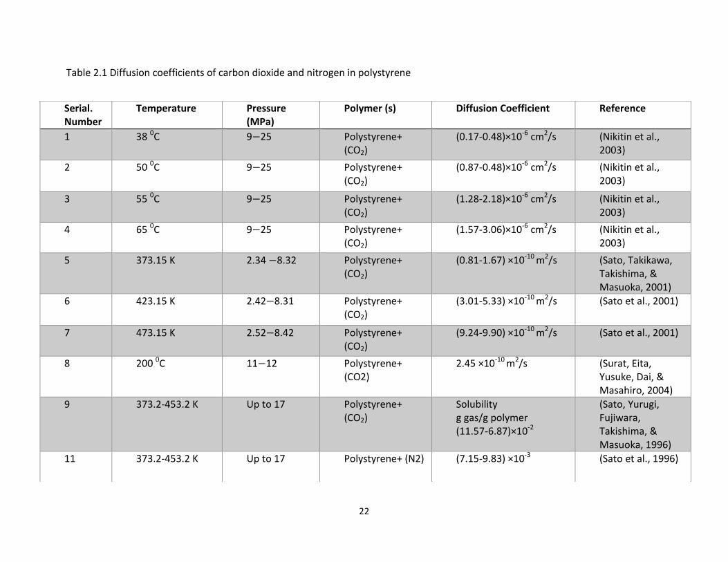
determination of concentration dependent diffusivities. Table 2.1 summarizes the previous
work done by other researchers in determining the diffusivities of carbon dioxide and
nitrogen in polystyrene.
22
Table 2.1 Diffusion coefficients of carbon dioxide and nitrogen in polystyrene
Serial. Number
Temperature Pressure (MPa)
Polymer (s) Diffusion Coefficient Reference
1 38 0C 9 25 Polystyrene+ (CO2)
(0.17-0.48)×10-6 cm2/s (Nikitin et al., 2003)
2 50 0C 9 25 Polystyrene+ (CO2)
(0.87-0.48)×10-6 cm2/s (Nikitin et al., 2003)
3 55 0C 9 25 Polystyrene+ (CO2)
(1.28-2.18)×10-6 cm2/s (Nikitin et al., 2003)
4 65 0C 9 25 Polystyrene+ (CO2)
(1.57-3.06)×10-6 cm2/s (Nikitin et al., 2003)
5 373.15 K 2.34 8.32 Polystyrene+ (CO2)
(0.81-1.67) ×10-10 m2/s (Sato, Takikawa, Takishima, & Masuoka, 2001)
6 423.15 K 2.42 8.31 Polystyrene+ (CO2)
(3.01-5.33) ×10-10 m2/s (Sato et al., 2001)
7 473.15 K 2.52 8.42 Polystyrene+ (CO2)
(9.24-9.90) ×10-10 m2/s (Sato et al., 2001)
8 200 0C 11 12 Polystyrene+ (CO2)
2.45 ×10⁻¹⁰ m2/s (Surat, Eita, Yusuke, Dai, & Masahiro, 2004)
9 373.2-453.2 K Up to 17 Polystyrene+ (CO2)
Solubility g gas/g polymer (11.57-6.87)×10-2
(Sato, Yurugi, Fujiwara, Takishima, & Masuoka, 1996)
11 373.2-453.2 K Up to 17 Polystyrene+ (N2) (7.15-9.83) ×10-3 (Sato et al., 1996)
23
Our plan is to develop an optimal control framework to determine diffusivity versus
concentration surfaces in ternary systems of two gases and a liquid. Therefore, the aim of
this study was to develop an optimal control framework novel method for the experimental
determination of multi-component diffusivities for a ternary system of two gases and one
non-volatile, dense phase. The novel feature of this work is that it allows the natural
evolution of multi-component diffusivity verses concentration in agreement with
experimental data and subject to the detailed mathematical model. This is an inverse
problem that can be solved using the principles of optimal control.
In our study, principles of optimal control is used to extract the optimal, composition-
dependent, multi-component diffusivities (system property) as a function of another
system property (composition).
2.2 Optimal Control
Optimization is a method of finding the conditions that give maximum or minimum value of
a function. But, if optimization involves minimization or maximization of a functional
subject to some constraint, the decision variable will not be a number, but will be a
function. Such problems are called optimal control problems. A functional is defined as a
function of several other functions. Optimal control problems involve two kinds of
variables: state and control variables. These variables are usually related to each other by a

24
set of differential equations. Optimal control theory can be used to solve such problems
(Upreti, 2013).
An optimal control technique solves the problem in number of stages, where each stage
develops from the preceding stage in prescribed manner. The control variables define the
system that governs the advancement of the system from one stage to the next. The state
variables describe the behaviour or status of the system at any stage. So, optimal control
problem is to find a set of control variables so that the total objective functional over all
the stages is optimized subject to a set of constraints (e.g. differential equation) on the
control and state variables.
Optimal control determines a control policy for a system that will maximize or minimize a
specific performance criterion subject to constrains. Optimal control has applications in
many different fields, including aerospace, process control, and engineering. In early 1950s
due to the lack of fast computers only simple optimal control problems could be solved.
The revolution of the digital computers in the 1950s, allows the application of optimal
control theory and methods to solve complex optimal control problems. Many applications
of optimal control theory were developed to optimization surfactant flooding process,
polymer process, and miscible carbon dioxide process (Ramirez, 1987). Although only initial
studies are present, promising advances are expected in the application of optimal control
theory.
A branch of mathematics that is useful in solving optimal control problems is the calculus of
variations (Denn, 1969; Kirk, 1970; Ray, 1981). Calculus of variations deals with functionals,
25
or functions whose independent variables are functions themselves. To solve optimal
control problems where the objective is to determine a function that minimize or maximize
a specified functional, calculus of variations is a useful technique.
The analogous problem in calculus is to determine a point that yields the minimum or
maximum value of a function. The variation plays the same role in determining extreme
values of functionals as the differential does in finding maxima and minima of functions.
The fundamental theorem used in finding extreme values of a function is the necessary
condition that the differential vanishes at an extreme point. In variational problems, the
analogous theorem is that the variation must be zero on an extrema.
Consider following simple example of optimal control in which functionals are formed as
integrals involving an unknown function and its derivatives:
∫
(2.1)
In Equation 2.1 is a functional of the function and . It is assumed that and are
initial and final time and are fixed, the end points of the curve are specified as and .
The objective is to find the control for which the functional has an optimum value
subject to the differential equation constraint which is given by
(2.2)
with the initial condition

26
(2.3)
At minimum of the variation of has to be zero.
∫ ( )
(2.4)
The above equation has to satisfy the differential equation constraint. The and
cannot be varied arbitrary because they are tied together in the differential objective
functional. According to optimal control theory, if the variations are arbitrary their
coefficients are individually zero. But in this case this is not possible because the control
and the state variable are tied together. This problem can be solved by introducing an
undetermined function, , called Lagrange multiplier, in the augmented objective
functional defined as
∫
(2.5)
At the optimum the variation of has to be zero
∫
( ) (2.6)
where the role of the lambda is to untie state variable from control by assuming certain
values in the time interval . With such values of lambda we are then able to vary
and arbitrary and independent of each other. This leads to simplified necessary
condition for the optimum of which is equal to the constraind optimum of . The
27
condition would add an equation for , the satisfaction of which enables the arbitrary
variations in the first place (Upreti, 2013).
To solve an optimal control problem, we must first describe the problem in physical terms,
and then translate the physical description into mathematical terms. Once the optimal
problem is defined mathematically, we can apply the optimal control theory to the partial
differential equations describing the process model.
28
3 EXPERIMENTAL SETUP
This chapter describes the experimental setup used for determining the concentration
dependent multi-component diffusivities of nitrogen and carbon dioxide in polystyrene.
Figure 3.1 shows the experimental setup used to determine the concentration-dependent
diffusivities of nitrogen and carbon dioxide in polystyrene. The setup was used to conduct
two kinds of experiments, i.e., solubility experiments and diffusion experiments.
The purpose of the solubility experiments was to determine the equilibrium concentration
of each gas at the gas–polymer interface as a function of pressure and gas-phase
composition. This information provides the boundary condition for the mass transfer
model of the diffusion process. The latter is conducted in diffusion experiments to furnish
experimental pressure and gas-phase composition as a function of time.
Figure 3.1 shows the main parts of the setup. It consists of a diffusion cell with a concentric,
4-cm-diameter cylindrical slot at the bottom to hold a polymer sample.

29
Figure 3.1. Experimental setup
Sampling nozzle
B A C
Vacuum
pump
To data acquisition system
Pressure transmitter
Mixture of nitrogen and carbon dioxide
Pressure vessel
Magnetic stirrer base
Pressure gauge
Polymer melt
Magnetic micro mixer
mixer
Laser sensor
D E
F
30
In an experiment, a mixture of nitrogen and carbon dioxide was allowed to diffuse into the
polymer layer inside a closed diffusion cell at a constant temperature.
The dimensions of the diffusion vessel are given in Table 3.1
Table 3.1 Diffusion vessel dimensions and material
Diameter 0.04 m
Volume
Depth 0.02 m
Mass of Polystyrene
Density of Polystyrene
1060
Carbon
dioxide
Obtained from MEGS specialty gases and equipment, Montreal (99.9 % pure)
Nitrogen Obtained from MEGS specialty gases and equipment, Montreal (99.9 % pure)
Polystyrene Sigma Aldrich (99.9% pure)
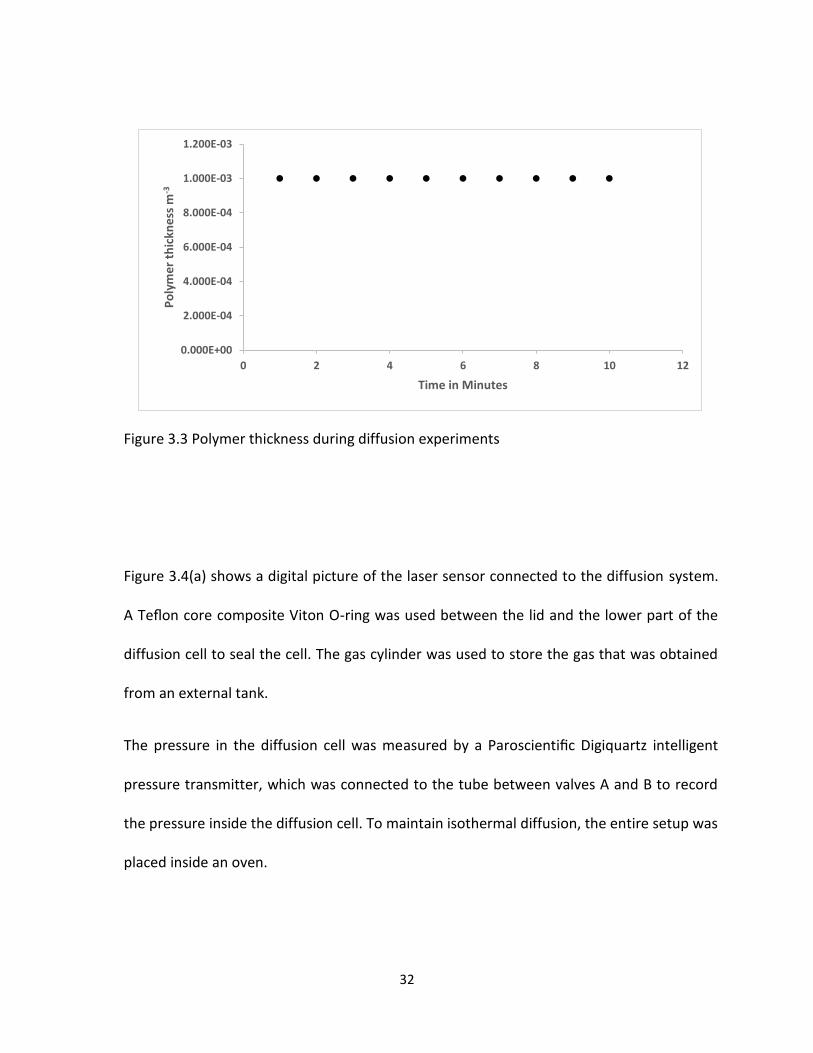
The lid of the diffusion cell had a glass window that allowed a complete view of the surface
of the polymer to an external, online, Keyence LKG displacement laser sensor, which
tracked the polymer’s surface. The laser beam detects any displacement in the thickness of
the polymer. The laser sensor has an accuracy of 10 µm that could lead to an error of 1.2%.
In our experiments, as expected, the laser sensor did not detect any change in the
thickness of the polymer because the experiments were done at room temperature (230C)
and low pressure. Figure 3.2 shows constant temperature inside the polymer during
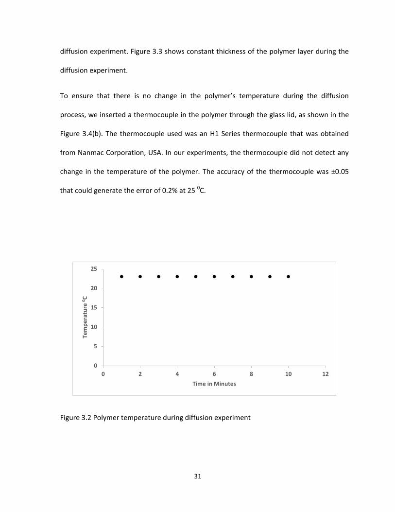
31
diffusion experiment. Figure 3.3 shows constant thickness of the polymer layer during the
diffusion experiment.
To ensure that there is no change in the polymer’s temperature during the diffusion
process, we inserted a thermocouple in the polymer through the glass lid, as shown in the
Figure 3.4(b). The thermocouple used was an H1 Series thermocouple that was obtained
from Nanmac Corporation, USA. In our experiments, the thermocouple did not detect any
change in the temperature of the polymer. The accuracy of the thermocouple was ±0.05
that could generate the error of 0.2% at 25 0C.
Figure 3.2 Polymer temperature during diffusion experiment
0
5
10
15
20
25
0 2 4 6 8 10 12
Tem
pe
ratu
re 0
C
Time in Minutes
32
Figure 3.3 Polymer thickness during diffusion experiments
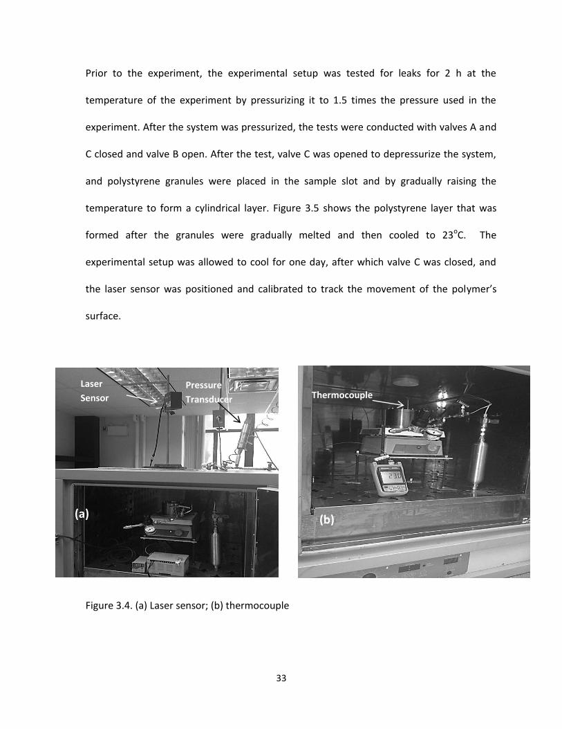
Figure 3.4(a) shows a digital picture of the laser sensor connected to the diffusion system.
A Teflon core composite Viton O-ring was used between the lid and the lower part of the
diffusion cell to seal the cell. The gas cylinder was used to store the gas that was obtained
from an external tank.
The pressure in the diffusion cell was measured by a Paroscientific Digiquartz intelligent
pressure transmitter, which was connected to the tube between valves A and B to record
the pressure inside the diffusion cell. To maintain isothermal diffusion, the entire setup was
placed inside an oven.
0.000E+00
2.000E-04
4.000E-04
6.000E-04
8.000E-04
1.000E-03
1.200E-03
0 2 4 6 8 10 12
Po
lym
er
thic
kne
ss m
-3
Time in Minutes
33
Prior to the experiment, the experimental setup was tested for leaks for 2 h at the
temperature of the experiment by pressurizing it to 1.5 times the pressure used in the
experiment. After the system was pressurized, the tests were conducted with valves A and
C closed and valve B open. After the test, valve C was opened to depressurize the system,
and polystyrene granules were placed in the sample slot and by gradually raising the
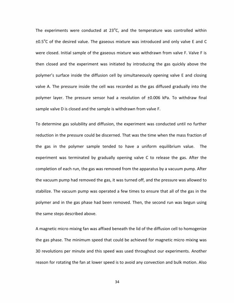
temperature to form a cylindrical layer. Figure 3.5 shows the polystyrene layer that was
formed after the granules were gradually melted and then cooled to 23oC. The
experimental setup was allowed to cool for one day, after which valve C was closed, and
the laser sensor was positioned and calibrated to track the movement of the polymer’s
surface.
Figure 3.4. (a) Laser sensor; (b) thermocouple
Thermocouple Laser
Sensor
Pressure
Transducer
(b)
(b)
(b)
(a)
34
The experiments were conducted at 23oC, and the temperature was controlled within
±0.5oC of the desired value. The gaseous mixture was introduced and only valve E and C
were closed. Initial sample of the gaseous mixture was withdrawn from valve F. Valve F is
then closed and the experiment was initiated by introducing the gas quickly above the
polymer’s surface inside the diffusion cell by simultaneously opening valve E and closing
valve A. The pressure inside the cell was recorded as the gas diffused gradually into the
polymer layer. The pressure sensor had a resolution of ±0.006 kPa. To withdraw final
sample valve D is closed and the sample is withdrawn from valve F.
To determine gas solubility and diffusion, the experiment was conducted until no further
reduction in the pressure could be discerned. That was the time when the mass fraction of
the gas in the polymer sample tended to have a uniform equilibrium value. The
experiment was terminated by gradually opening valve C to release the gas. After the
completion of each run, the gas was removed from the apparatus by a vacuum pump. After
the vacuum pump had removed the gas, it was turned off, and the pressure was allowed to
stabilize. The vacuum pump was operated a few times to ensure that all of the gas in the
polymer and in the gas phase had been removed. Then, the second run was begun using
the same steps described above.
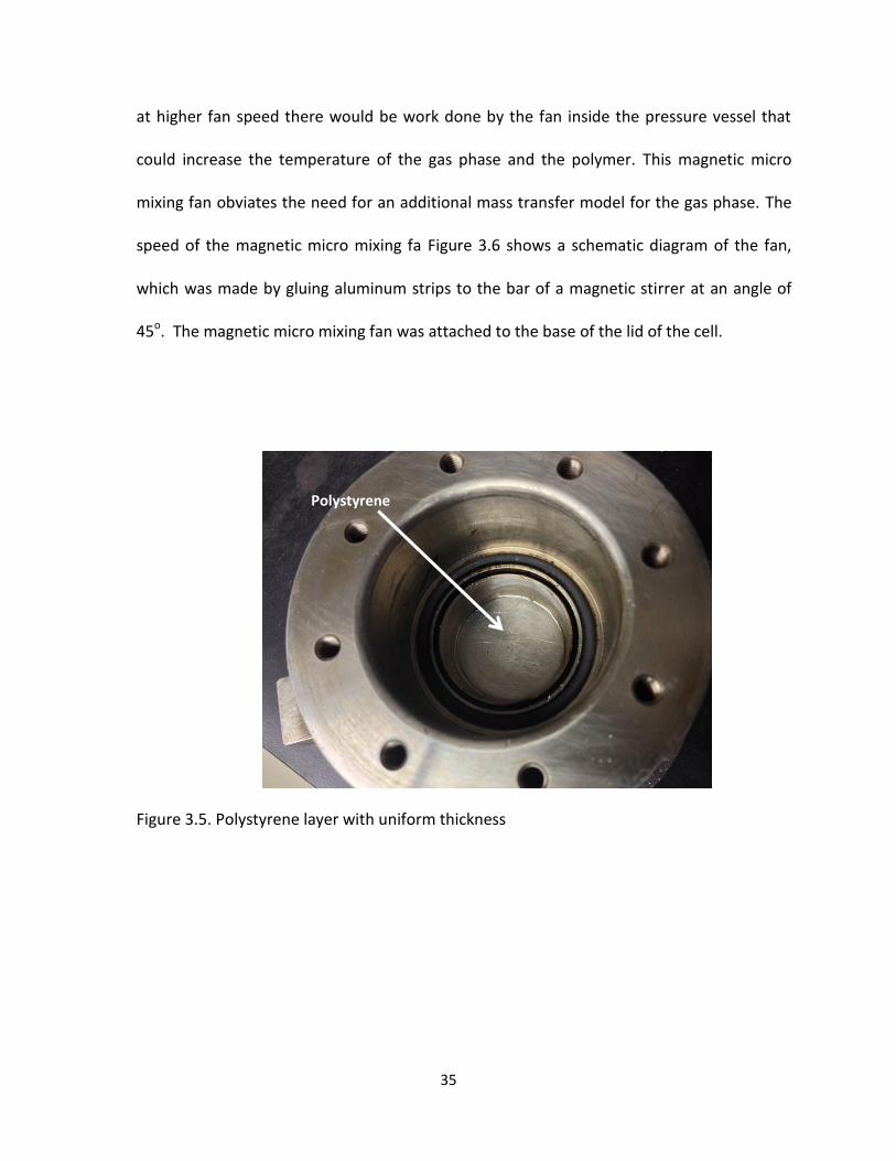
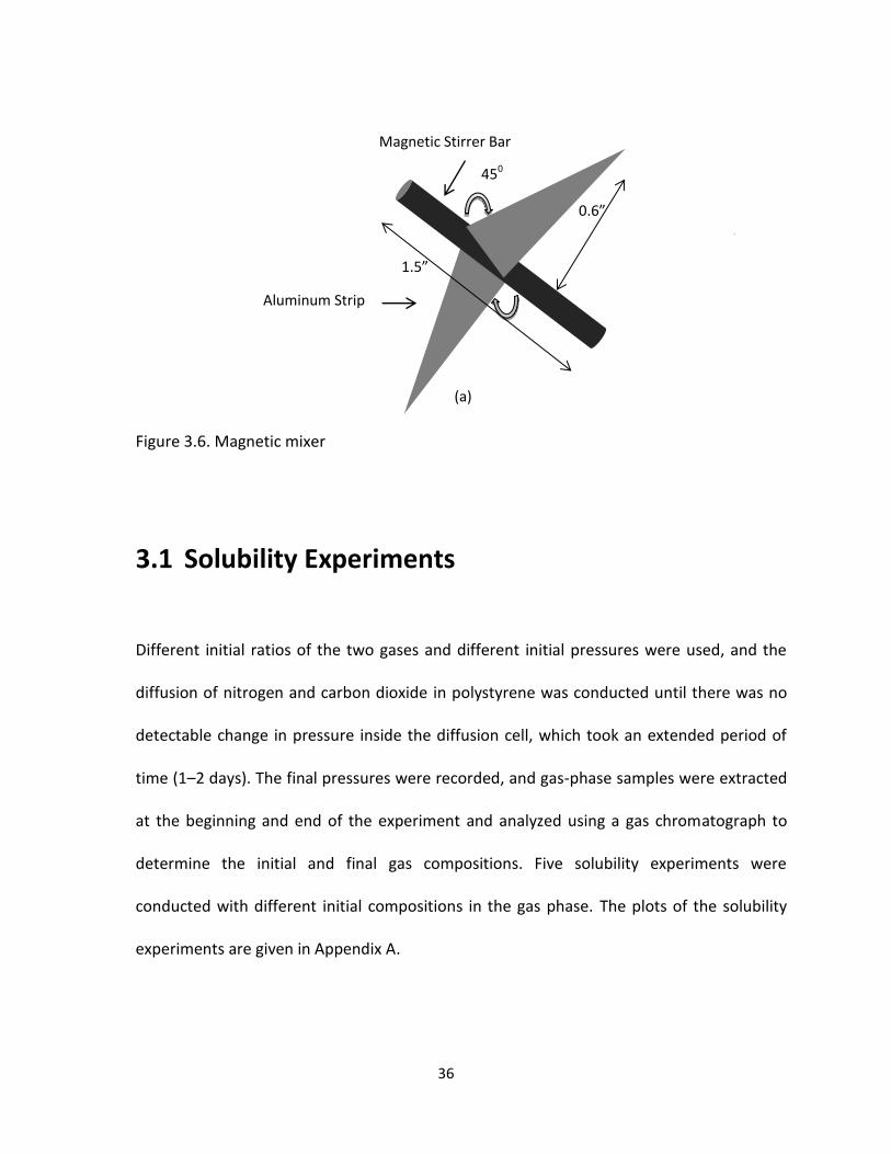
A magnetic micro mixing fan was affixed beneath the lid of the diffusion cell to homogenize
the gas phase. The minimum speed that could be achieved for magnetic micro mixing was
30 revolutions per minute and this speed was used throughout our experiments. Another
reason for rotating the fan at lower speed is to avoid any convection and bulk motion. Also
35
at higher fan speed there would be work done by the fan inside the pressure vessel that
could increase the temperature of the gas phase and the polymer. This magnetic micro
mixing fan obviates the need for an additional mass transfer model for the gas phase. The
speed of the magnetic micro mixing fa Figure 3.6 shows a schematic diagram of the fan,
which was made by gluing aluminum strips to the bar of a magnetic stirrer at an angle of
45o. The magnetic micro mixing fan was attached to the base of the lid of the cell.
Figure 3.5. Polystyrene layer with uniform thickness
Polystyrene
36
Figure 3.6. Magnetic mixer
3.1 Solubility Experiments
Different initial ratios of the two gases and different initial pressures were used, and the
diffusion of nitrogen and carbon dioxide in polystyrene was conducted until there was no
detectable change in pressure inside the diffusion cell, which took an extended period of
time (1–2 days). The final pressures were recorded, and gas-phase samples were extracted
at the beginning and end of the experiment and analyzed using a gas chromatograph to
determine the initial and final gas compositions. Five solubility experiments were
conducted with different initial compositions in the gas phase. The plots of the solubility
experiments are given in Appendix A.
0.6”
1.5”
Aluminum Strip
450
Magnetic Stirrer Bar
(a)
37
The purpose of these experiments was to determine the interfacial (equilibrium)
concentration of nitrogen and carbon dioxide at the gas–polymer interface as a function of
pressure and gas-phase composition:
(3.1)
The
s formed the boundary conditions in the mass transfer model to be used for the
determination of the concentration-dependent, multi-component diffusivities of the gases
in the polymer. These masses provided the solubility or
s at the final pressures and gas-
phase compositions.
3.2 Diffusion Experiments
With a fixed initial ratio of the masses of the two gases and a fixed initial pressure, the
diffusion process was conducted for 2, 4, 6, 8, and 10 minutes. The composition of the gas
phase was determined at the beginning and the end of each experiment using a gas
chromatograph.
The purpose of these experiments was to obtain data for pressure and gas-phase
composition as a function of time, i.e., and . These data provided:
1. The experimental values of the masses of the two gases absorbed in the polymer as a
function of time.
38
2. The calculated counterparts of the above masses given by the mass transfer model, which
had:
(a) Boundary conditions that were obtained from solubility experiments:
(b) Composition-dependent diffusivities of each gas in polymer:
(
) (3.2)
3.3 Analysis of Gas Phase Composition
The gas-phase composition during the diffusion and solubility experiments was analyzed by
a gas chromatograph. Now, the gas chromatograph is introduced briefly, including how it
works, how the samples were extracted during the solubility and diffusion experiments, the
column used in this study, and the gas chromatography method that was used in the
analysis of the composition of the gas phase. A succinct introduction of the gas
chromatograph (GC) follows.
3.3.1 Gas Chromatography
Chromatography is the separation of a mixture of compounds (solutes) into separate
components, making it easier to identify (qualitate) and measure (quantitate) each
component. GC is one of several chromatographic techniques. It is appropriate for
39
analyzing 10–20% of all known compounds. To be suitable for GC analysis, a compound
must have sufficient volatility and thermal stability. If all or some of a compound’s
molecules are in the gas phase at 400–450 oC or below and they do not decompose at
these temperatures, the compound probably can be analyzed by GC.
3.3.2 Chromatogram
The size of the peak corresponds to the amount of the compound of interest in the sample.
As the amount of the compound of interest increases in the samples being analyzed, larger peaks
are attained for that compound. Retention time is the time it takes for a compound to travel
through the column. If the column and all operating conditions are kept constant, a given
compound will always have the same retention time.
Peak size and retention time are used for quantitative and qualitative analyses of a
compound, respectively. However, the identification of a compound cannot be determined
solely by its retention time. A known amount of an authentic, pure sample of the
compound must first be analyzed to determine its retention time and peak size. Then, this
value is compared to the results from an unknown sample to determine whether the target
compound is present (by comparing retention times) and in what quantity (by comparing
peak size).
In this study, thermal conductivity detector was used. Thermal conductivity detector relies
on the thermal conductivity of matter passing around a tungsten-rhenium filament with a
40
current traveling through it. In this set up helium is used as a carrier gas because of their
relatively high thermal conductivity which keep the filament cool and maintain uniform
resistivity and electrical efficiency of the filament. However, when analyte molecules elute
from the column, mixed with carrier gas, the thermal conductivity decreases and this
causes a detector response. The response is due to the decreased thermal conductivity
causing an increase in filament temperature and resistivity resulting in fluctuations in
voltage. Detector sensitivity is proportional to filament current while it is inversely
proportional to the immediate environmental temperature of that detector as well as flow
rate of the carrier gas.
A Varian gas chromatograph, model CP3800, with Galaxie V1.9 software, was used to
determine the amounts of carbon dioxide and nitrogen in the sample obtained from the
diffusion cell. The column HP-Plot Q, obtained from Agilent Technologies Canada, was used
for the detection of eluents from the gas chromatograph. The inner diameter of the column
was 0.32 mm, and the length of the column was 15 m. The stationary phase in the column
was polystyrene divinyl benzene.
3.3.3 Sampling
A gas-tight, high-performance, micro syringe with a volume of 1,000 µL, obtained from
Sigma-Aldrich, was used to draw the samples from the sampling nozzle. The sample in the
syringe was injected manually into the gas chromatograph column for detection.
41
Before we used the GC to determine the experimental masses of nitrogen and carbon
dioxide absorbed in the polystyrene, we ran pure samples of nitrogen and carbon dioxide
with different initial volumes. Then the areas under the peaks were plotted against the
volume of the samples. The best straight-line fit of the data was determined and for use in
determining the composition of these two gases in the unknown sample. The curve-fitting
plots are provided in Appendix B.
During the solubility and diffusion experiments, 200µL samples were injected manually
through the GC sample inlet at 240oC. The retention time was determined by a thermal
conductivity detector that was maintained at 240oC.
Helium was used as the carrier gas (mobile phase). The flow rate of the mobile phase was
8.6 mL/min. The oven that housed the GC column was maintained at 35oC.
Using the measured composition of the gas phase, we calculated the experimental mass of
each gas absorbed in the polystyrene at the time when the samples were extracted. The
detailed calculation is given in Appendix B.
42
4 THEORY and COMPUTATION
This chapter presents the development of optimal control framework to determine
concentration dependent multicomponent diffusivities of two gases in a non-volatile dense
phase, which is the primary objective of this study. Interfacial gas mass fractions of two
gases versus time are used as control in this optimal control problem. The optimal
diffusivities are then determined that minimises the error between the experimental the
calculated gas mass absorbed.
The optimal control framework to determine the concentration dependent
multicomponent diffusivities is based on detailed mass transfer model, which comprises
continuity equation of diffusion. Optimal control principles are applied to derive necessary
conditions for which the error between the experimental and calculated gas mass absorbed
is minimum. A numerical algorithm is developed to estimate the optimal ternary
diffusivities.
4.1 Mass Transfer Model
The mathematical model was based on the following assumptions:
1. Mass transfer is along the depth of the dense phase.
43
The polymer is in the pressure-decay vessel and only its surfaces are exposed to the
diffusing gases. The other three sides of the polymer are adhered to the base or the walls
of the pressure-decay vessel. Based on these facts, it can be assumed that the diffusion of
the gases in the polymer melt is only in the downward direction (z-direction). Hence, it is a
unidirectional diffusion process.
2. No chemical reactions occur in the pressure vessel.
The absorption of the gases in the polymer melt is purely a physical phenomenon. There
are no reactions among carbon dioxide, nitrogen, and the polymer melt at the temperature
and pressure of the experiment.
3. Diffusion occurs at constant temperature.
While the diffusion of the gases is occurring, the temperature of the pressure-decay system
and its components does not change. (This assumption inherently means that any thermal
energy released during the diffusion is dissipated instantaneously to the surroundings
4. There is no convection in the dense, non-volatile phase.
The rotation of magnetic micro mixer was kept low at 30 rpm. Hence, it is assumed that
there is no diffusion due to convection or bulk motion in the gas phase due to the rotation
of the magnetic micro mixer inside the pressure-decay vessel. Also, at this low rotational
speed, the work done by the magnetic micro mixer does not affect the temperature inside
the pressure-decay vessel.
5. The wall effects are negligible.
It is assumed that the permeating gases (carbon dioxide and nitrogen) move only along the
z-direction i.e., the depth of the polymer.

44
6. The pressure decay is solely due to the diffusion of the gases and there is no leakage.
Before the experiment was started, it was ensured that the pressure-decay equipment had
no leaks. Hence, it is assumed that the decrease in the pressure is solely due to diffusion.
7. The gas phase is homogenous at all times.
Since the magnetic micro mixer was constantly moving at slow speed above the surface of
the polymer. So, it is assumed that the gas phase is homogenous at all times.
Figure 4.1 shows the diffusion of nitrogen and carbon dioxide in polystyrene. Dark colored
circles represent carbon dioxide and the white color circles represent nitrogen. The two
gases diffuse in the polymer of depth of z. The diffusivity of the two gases is a function of
the mass fraction of the two gases .
Figure 4.1. Diffusion of two gases in an underlying dense, non-volatile phase
Carbon dioxide Nitrogen z = L = length
Gas Phase
= (z, t) z=L
Polymer
z=0

45
4.2 Theoretical Model Development
Considering the assumptions mentioned above, the mass transfer model is presented
below. We use subscripts ‘1’ and ‘2’ for the nitrogen and carbon dioxide respectively, and
‘3’ for the non-volatile phase. For the first gas:
011
z
N
t
ω, (4.1)
where 1 is the mole fraction of the first gas, and
1N is the mass flux of that gas, both in
the underlying layer of the dense, non-volatile phase; the flux is given by:
13121111JNωNωNωN (4.2)
where 2
N and 3N are the mass flux of the second gas and the dense non-volatile phase,
respectively. Since 3
N is zero, Equation (4.2) becomes:
DJNωNωN
21111 (4.3)
where 1J is the diffusive flux for the first gas, and it is given by:
z
ωD
z
ωDJ
D
2
12
1
11 (4.4)
z
ωD
z
ωDNω
ωN 2
12
1
1121
1
11
1 (4.5)
Similarly for the second gas, we have
z
ωD
z
ωDNω
ωN 1
21
2
2212
2
21
1 (4.6)
Substituting Equation (4.6) in Equation (4.5), we get:

46
z
ωD
z
ωD
z
ωD
z
ωDNω
ωω
ωN 2
12
1
11
1
21
2
2212
2
1
1
11
1
1
1 (4.7)
Simplifying for we get
z
ωD
z
ωD
ωz
ωD
z
ωD
ωω
ωN
ωω
ωωN 2
12
1
11
1
1
21
2
22
21
1
1
21
21
11
1
1111 (4.8)
z
ωD
z
ωD
ωz
ωD
z
ωD
ωω
ω
ωω
ωωN 2
12
1
11
1
1
21
2
22
21
1
21
21
11
1
11
111
1 (4.9)
z
ωD
z
ωD
ω
z
ωD
z
ωD
ωω
ω
ωωωω
ωωN
2
12
1
11
1
1
21
2
22
21
1
2121
21
1
1
1
11
11
11 (4.10)
z
ωD
z
ωD
z
ωD
z
ωD
ω
ω
ωω
ωN 2
12
1
11
1
21
2
22
2
1
21
2
111
1 (4.11)
Now substituting Equation (4.11) into Equation (4.1), we get
z
ωD
z
ωD
z
ωD
z
ωD
ω
ω
ωω
ω
zt
ω2
12
1
11
1
21
2
22
2
1
21
21
11
1 (4.12)
or
z
ωD
z
ωD
ωω
ω
zz
ωD
z
ωD
ωω
ω
zt
ω2
12
1
11
21
21
21
2
22
21
11
1
1
1 (4.13)
47
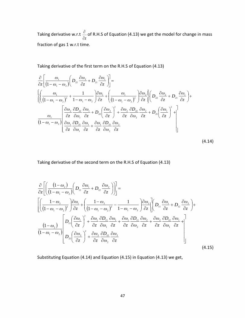
Taking derivative w.r.t z
of R.H.S of Equation (4.13) we get the model for change in mass
fraction of gas 1 w.r.t time.
Taking derivative of the first term on the R.H.S of Equation (4.13)
z
ω
ω
D
z
ω
z
ω
ω
D
z
ω
z
ωD
z
ω
ω
D
z
ω
z
ωD
z
ω
ω
D
z
ω
ωω
ω
z
ωD
z
ωD
z
ω
ωω
ω
z
ω
ωωωω
ω
z
ωD
z
ωD
ωω
ω
z
2
2
2111
1
211
2
1
21
2
2
222
2
2
22
1
1
222
21
1
1
21
2
22
2
2
21
11
21
2
21
1
1
21
2
22
21
1
1
11
1
1
1
(4.14)
Taking derivative of the second term on the R.H.S of Equation (4.13)
z
ω
ω
D
z
ω
z
ωD
z
ω
ω
D
z
ω
z
ω
ω
D
z
ω
z
ω
ω
D
z
ω
z
ωD
ωω
ω
z
ωD
z
ωD
z
ω
ωωωω
ω
z
ω
ωω
ω
z
ωD
z
ωD
ωω
ω
z
2
2
122
2
2
21
1
1
1222
2
1111
1
111
2
1
11
21
2
2
12
1
11
2
21
2
21
21
2
21
2
2
12
1
11
21
2
1
1
1
1
1
1
1
1
1
1
(4.15)
Substituting Equation (4.14) and Equation (4.15) in Equation (4.13) we get,

48
z
ω
ω
D
z
ω
z
ωD
z
ω
ω
D
z
ω
z
ω
ω
D
z
ω
z
ω
ω
D
z
ω
z
ωD
ωω
ω
z
ωD
z
ωD
z
ω
ωωωω
ω
z
ω
ωω
ω
z
ω
ω
D
z
ω
z
ω
ω
D
z
ω
z
ωD
z
ω
ω
D
z
ω
z
ωD
z
ω
ω
D
z
ω
ωω
ω
z
ωD
z
ωD
z
ω
ωω
ω
z
ω
ωωωω
ω
t
ω
2
2
122
2
2
2
21
1
1
1222
2
1111
1
111
2
1
2
11
21
2
2
12
1
11
2
21
2
21
21
2
21
2
2
2
2111
1
211
2
1
2
21
2
2
222
2
2
2
22
1
1
222
21
1
1
21
2
22
2
2
21
11
21
2
21
11
1
1
1
1
1
1
1
1
1
11
1
1
(4.16)
Or
2
2
2
21
2
21
21
1
222
1
2
11
21
2
21
1
21
2
2
12
1
11
21
2
21
21
21
2
222
21
1
1
2
12
1
112
21
2
1
21
2
22
21
2
21
1
1
1
z
ω
ωω1
ω1D
ωω1
ωD
z
ωD
ωω1
ω1
ωω1
ωD
z
ω
z
ωD
z
ωD
ωω1
1
ωω1
ω1
z
ωD
z
ωD
ωω1
ω
z
ω
z
ωD
z
ωD
ωω1
ω1
z
ωD
z
ωD
ωω1
1
ωω1
ω
t
ωf
49
2
2
2
22
21
1
2
12
21
2
2
1
1
11
21
2
1
21
21
1
21
1
12
21
2
2
11
21
2
2
21
21
1
1
22
21
1
z
ω
ω
D
ωω1
ω
ω
D
ωω1
ω1
z
ω
ω
D
ωω1
ω1
ω
D
ωω1
ω
z
ω
z
ω
ω
D
ωω1
ω1
ω
D
ωω1
ω1
ω
D
ωω1
ω
ω
D
ωω1
ω
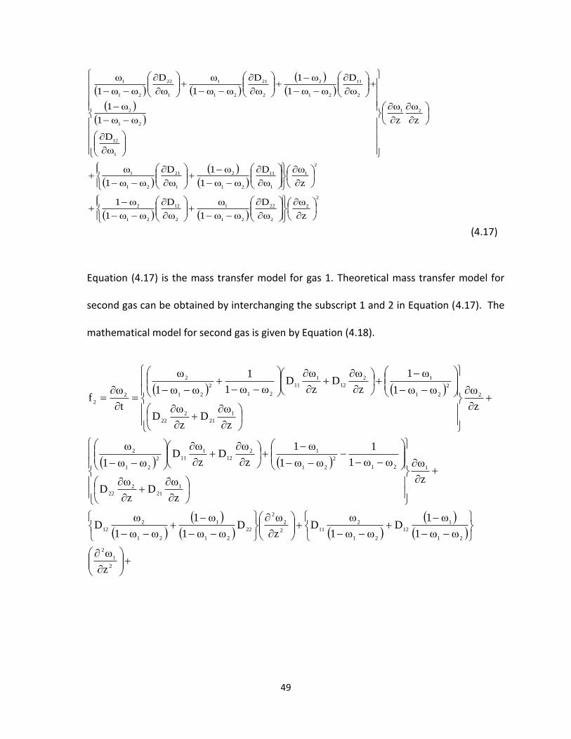
(4.17)
Equation (4.17) is the mass transfer model for gas 1. Theoretical mass transfer model for
second gas can be obtained by interchanging the subscript 1 and 2 in Equation (4.17). The
mathematical model for second gas is given by Equation (4.18).
2
1
2
21
1
12
21
2
112
2
2
22
21
1
21
2
12
1
1
21
2
22
21
2
21
12
12
1
112
21
2
2
1
21
2
22
2
21
12
12
1
11
21
2
21
2
2
2
z
ω
ωω1
ω1D
ωω1
ωD
z
ωD
ωω1
ω1
ωω1
ωD
z
ω
z
ωD
z
ωD
ωω1
1
ωω1
ω1
z
ωD
z
ωD
ωω1
ω
z
ω
z
ωD
z
ωD
ωω1
ω1
z
ωD
z
ωD
ωω1
1
ωω1
ω
t
ωf
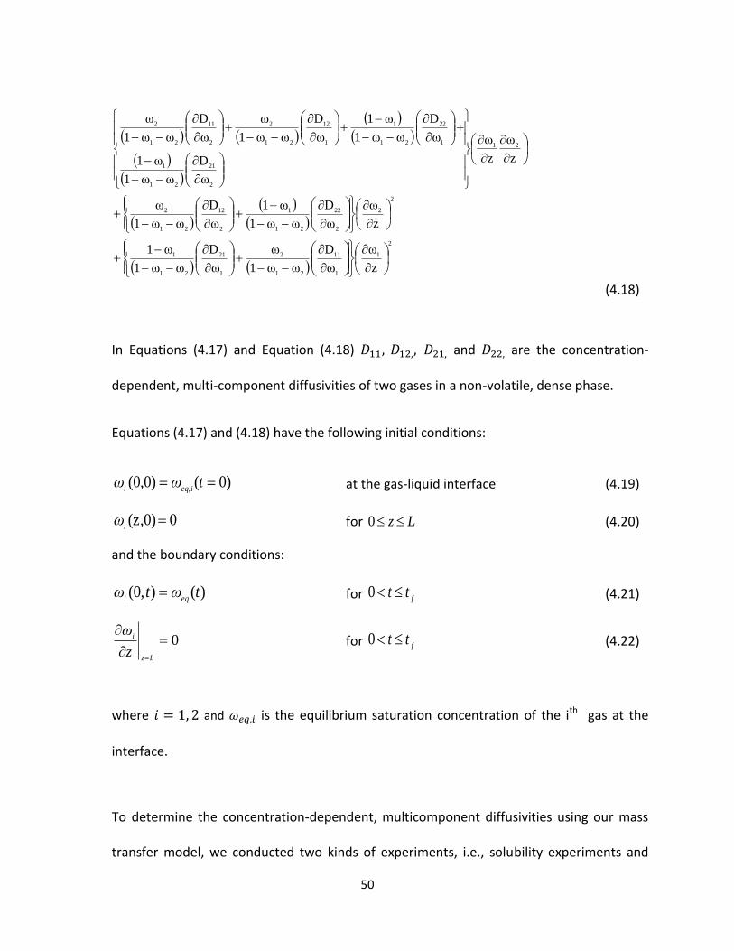
50
2
1
1
11
21
2
1
21
21
1
2
2
2
22
21
1
2
12
21
2
21
2
21
21
1
1
22
21
1
1
12
21
2
2
11
21
2
z
ω
ω
D
ωω1
ω
ω
D
ωω1
ω1
z
ω
ω
D
ωω1
ω1
ω
D
ωω1
ω
z
ω
z
ω
ω
D
ωω1
ω1
ω
D
ωω1
ω1
ω
D
ωω1
ω
ω
D
ωω1
ω
(4.18)
In Equations (4.17) and Equation (4.18) and are the concentration-
dependent, multi-component diffusivities of two gases in a non-volatile, dense phase.
Equations (4.17) and (4.18) have the following initial conditions:
0)((0,0) tωωeq,ii at the gas-liquid interface (4.19)
0(z,0)i
ω for Lz 0 (4.20)
and the boundary conditions:
)()(0, tωtωeqi
for ftt 0 (4.21)
0
Lz
i
z
ω for f
tt 0 (4.22)
where and is the equilibrium saturation concentration of the ith gas at the
interface.
To determine the concentration-dependent, multicomponent diffusivities using our mass
transfer model, we conducted two kinds of experiments, i.e., solubility experiments and
51
diffusion experiments. The purpose of the solubility experiments was to determine the
equilibrium concentration of each gas at the gas–polymer interface as a function of
pressure and gas-phase composition. This provided the boundary conditions. The purpose
of the diffusion experiments was to obtain data for pressure and the gas-phase
composition as a function of time. These data provided the experimental mass of each gas
absorbed in the dense phase.
To solve our mass transfer model, the four unknown diffusivities, and
are required. This is an inverse problem that can be solved using the optimal control
technique.
4.3 Optimal Control
An optimal control involves the improvement in the system’s performance as a function of
time, space, or any other independent variable. In our study, the optimal control technique
was used to extract the optimal, composition-dependent, multi-component diffusivities
(system property) as a function of another system property (composition). Unknown
diffusivities are control surfaces that must be optimally determined such that the
difference between the experimental and calculated masses is minimized. The error
function is the objective function that is described next (Upreti, 2013).

52
4.4 The Objective Functional
The goal is to determine the unknown, concentration-dependent, multi-component
diffusivities of the two gases in the non-volatile dense phase such that their use in
equations (4.19) to (4.22) yields the calculated masses of the gases in the layer that are in
agreement with experimentally-determined masses of the gases, i.e., (t)m1exp and (t)m
2exp
through gas chromatograph and pressure decay measurements. The objective functional
can be expressed as the summation of:
dttmtmIT 2
0exp1mod11 (4.23)
and
dttmtmIT 2
0exp2mod22 (4.24)
where 1I and
2I are the measures of error between the predicted and experimental gas
masses for the respective gases over time T.
At any given time, tmmod1 and tm
mod1 are the model-predicted mass of gases absorbed in
the polymer, whereas, tm1exp and tm2exp are the experimental-determined gas masses
absorbed in the polymer. The model-predicted mass of each gas absorbed is given by:
L
Adzρωm0
1mod1 and, L
Adzρωm0
2mod2 (4.25)
53
Thus,
dt)mρAdz(ω)mρAdz(ωIIIT L
0 0
2
exp22
2
exp1121 (4.26)
where L is the depth of the polymer phase having a cross-sectional area A. Note that
is given by the highly non-linear, partial differential Equations (4.17) and (4.18),
having diffusivities as the two-
dimensional surfaces to be optimally determined.
The optimal control problem is to determine these functions that minimizes given by
Equation (4.26) subject to the satisfaction of differential equation constraints. So, Equation
(4.17) can also be written as:
0
222112112
2
2
2
1
2
21
211
1
1,D,D,D,D
z
ω,
z
ω,
z
ω,
z
ω,,ωωf
t
ω(z,t)G
(4.27)
For the second gas, Equation (4.18) can be written as:
0222112112
2
2
2
1
2
21
212
2
2
,D,D,D,D
z
ω,
z
ω,
z
ω,
z
ω,,ωωf
t
ω(z,t)G
(4.28)
The constrained problem above is equivalent to the unconstrained minimization of:
)dzdtGλG(λIIJT L
0
220
1121
(4.29)
where is the augmented objective functional and )(z,tλi is a costate variable
54
In the next section, we derive necessary condition for J to be at its minimum value. The
solution of necessary conditions will yield the unknown concentration dependent
multicomponent diffusivities.
4.5 Necessary Condition for the Minimum
The necessary condition for the minimum is that the variation of J is zero, i.e.:
00
22220
111121 )dzdtδGλGδλδGλG(δδδIδIδJ
T L
(4.30)
In the above equation:
T L
dzdtδωmmAρδI0
10
exp1mod112
(4.31)
T L
dzdtδωmmAρδI0
20
exp2mod222 (4.32)
1δG and
2δG , respectively, are given by:
22
22
1
21
21
1
12
12
1
11
11
1
2
2
1
1
1
1
2
2
1
1
1
1
2
2
1
1
1
1
11
δDD
fδD
D
fδD
D
f
δDD
fδω
ω
fδω
ω
fδω
ω
fδω
ω
fδω
ω
fδω
ω
fδω
tδG
ZZ
ZZ
ZZ
ZZ
Z
Z
Z
Z
(4.33)
55
22
22
2
21
21
2
12
12
2
11
11
2
1
1
2
2
2
2
1
1
2
2
2
2
1
1
2
2
2
2
22
δDD
fδD
D
fδD
D
f
δDD
fδω
ω
fδω
ω
fδω
ω
fδω
ω
fδω
ω
fδω
ω
fδω
tδG
ZZ
ZZ
ZZ
ZZ
Z
Z
Z
Z
(4.34)
Substituting Equations (4.31-4.34) into Equation (4.30) we get:
2
22
22
2
21
21
2
12
12
2
11
11
2
1
1
2
2
2
2
1
1
2
2
2
2
1
1
2
2
2
2
20 0
2
1
22
22
1
21
21
1
12
12
1
11
11
1
2
2
1
1
1
1
2
2
1
1
1
1
2
2
1
1
1
1
10 0
1
0 0
2
22expmod
1
11expmod22
Gas
ZZ
ZZ
ZZ
ZZ
Z
Z
Z
Z
T L
Gas
ZZ
ZZ
ZZ
ZZ
Z
Z
Z
Z
T L
T L
GasGas
)dzdtδDD
fδD
D
fδD
D
fδD
D
f
δωω
f
δωω
fδω
ω
fδω
ω
fδω
ω
fδω
ω
fδω
t(λ
)dzdtδDD
fδD
D
fδD
D
fδD
D
fδω
ω
f
δωω
fδω
ω
fδω
ω
fδω
ω
fδω
ω
fδω
t(λ
dzdtδωmmAρδωmmAρδJ
(4.35)
variation δJ is a combination of 1
δJ (for gas 1) and 2
δJ (for gas 2).
21δJδJδJ
where 1
δJ and 2
δJ are given by

56
)dzdtδDD
f
δDD
fδD
D
fδD
D
fδω
ω
fδω
ω
fδω
ω
f
δωω
fδω
ω
fδω
ω
fδω
t(λdzdtδωmmAρδJ
ZZ
ZZ
ZZ
ZZ
Z
Z
Z
Z
T LT L
22
22
1
21
21
1
12
12
1
11
11
1
2
2
1
1
1
1
2
2
1
1
1
1
2
2
1
1
1
1
10 0
10 0
11expmod12
(4.36)
and
)dzdtδDD
f
δDD
fδD
D
fδD
D
fδω
ω
fδω
ω
fδω
ω
f
δωω
fδω
ω
fδω
ω
fδω
t(λdzdtδωmmAρδJ
ZZ
ZZ
ZZ
ZZ
Z
Z
Z
Z
T LT L
22
22
2
21
21
2
12
12
2
11
11
2
1
1
2
2
2
2
1
1
2
2
2
2
1
1
2
2
2
2
20 0
20 0
22expmod22
(4.37)
For the sake of simplicity we first simplify the terms on the R.H.S of Equation (4.36) for gas
1:
Integrating by parts the third, sixth, seventh, eighth, and ninth terms in the Equation (4.36),
we get:
dzdtδωλdzδωt
λ)dzdtδωt
(λT L
T
LT L
10 0
1
0
011
0 011
(4.38)
dzdtδωω
fλ
zdtδω
ω
fλ)dzdtδω
ω
f(λ
Z
T LL
T
Z
T L
Z
Z
1
1
1
10 0
00
1
1
1
10 0
1
1
1
1
(4.39)
dzdtδωω
fλ
zdtδω
ω
fλ)dzdtδω
ω
f(λ
Z
T LL
T
Z
T L
Z
Z
2
2
1
10 0
00
2
2
1
10 0
2
2
1
1
(4.40)
57
dzdtδωω
fλ
zdtδω
ω
fλ
zdtδω
ω
fλ)dzdtδω
ω
f(λ
ZZ
T LT
L
ZZ
LT
Z
ZZ
T L
ZZ
ZZ
1
1
1
10 0
2
2
00
1
1
1
1
00
1
1
1
10 0
1
1
1
1
(4.41)
dzdtδωω
fλ
zdtδω
ω
fλ
zdtδω
ω
fλ)dzdtδω
ω
f(λ
ZZ
T LT
L
ZZ
LT
Z
ZZ
T L
ZZ
ZZ
2
2
1
10 0
2
2
00
2
2
1
1
00
2
2
1
10 0
2
2
1
1
(4.42)
Substituting Equations (4.38-3.42) into Equation (4.36) and rearranging gives:
dzdt)δDD
fλδD
D
fλδD
D
fλδD
D
fλ
dtδωω
fλdtδω
ω
fλ
dtδωω
fλ
zω
fλ
dzδωλ
dtδωω
fλ
zω
fλ
dzdtδωω
fλ
zω
fλ
zω
fλ
dzδωω
fλ
zω
fλ
zω
fλdzdtλ
tδIδJ
T L
Z
LT
ZZ
Z
LT
ZZ
L
T
ZZZ
TL
L
T
ZZZ
T L
ZZZ
T L
ZZZ
0 022
22
1
121
21
1
112
12
1
111
11
1
1
2
00
2
1
11
00
1
1
1
2
00
2
1
1
2
1
1
0011
1
00
1
1
1
1
1
1
20 0
2
1
12
2
2
1
1
2
1
1
0 01
1
1
12
2
1
1
1
11
1
1111
(4.43)
Similarly, 2J can be derived by interchanging subscripts 1 and 2 in Equation (4.43).
Because the initial mass concentration of the gas in the polymer is known at the interface
and is zero everywhere in the polymer, the variation )0,(1 z and )0,(2 z is zero for all
58
values of z . Since the final mass concentration of the gas is not specified, the fourth
integral in Equation (4.43) is eliminated by forcing:
0(z,T)λi Lz 0 (4.44)
Since the equilibrium concentration of gas at the interface (t)]ωt)(0,[ωsat11 and
(t)]ωt)(0,[ωsat22 is always specified, t)(0,δω1or2 is zero. Therefore, the third and fifth
integrals are eliminated in Equation (4.43). Furthermore, by forcing:
0(L,t)λi Tt 0
(4.45)
00 ,t)(λi Tt 0
(4.46)
the sixth terms in equation (4.43) are eliminated. Similarly variation of gas 2 2δJ can also be
simplified. Simplifying and rearranging Equation (4.35), we get:
59
dzdtδDD
fλδD
D
fλδD
D
fλδD
D
fλ
dzdtδDD
fλδD
D
fλδD
D
fλδD
D
fλ
dzdtδω
ω
fλ
zω
fλ
zω
fλ
ω
fλ
zω
fλ
zω
fλλ
tmmAρ
dzdtδω
ω
fλ
zω
fλ
zω
fλ
ω
fλ
zω
fλ
zω
fλλ
tmmAρ
δJ
T L
T L
T L
ZZZ
T L
ZZZ
T L
ZZZ
T L
ZZZ
0 022
22
2
221
21
2
212
12
2
211
11
2
2
0 022
22
1
121
21
1
112
12
1
111
11
1
1
2
0 02
1
12
2
2
1
1
2
1
1
0 02
2
12
2
2
2
2
2
2
222expmod
1
0 01
2
22
2
1
2
2
1
2
2
0 01
1
12
2
1
1
1
1
1
111expmod
2
2
(4.47)
In the above equation, the first integral is eliminated by defining t
λ
1 as follows:
ZZZ
ZZZ
ω
fλ
zω
fλ
zω
fλ
ω
fλ
zω
fλ
zω
fλmmAρ
t
λ
1
2
22
2
1
2
2
1
2
2
1
1
12
2
1
1
1
1
1
11expmod
1 2
(4.48)
and second integral in Equation (4.47) can be eliminated by defining t
λ
2 as follows:
ZZZ
ZZZ
ω
fλ
zω
fλ
zω
fλ
ω
fλ
zω
fλ
zω
fλmmAρ
t
λ
2
1
12
2
2
1
1
2
1
1
2
2
12
2
2
2
2
2
2
22expmod
2 2
(4.49)
60
Equation (4.44) is the initial condition for Equations (4.48) and (4.49), and Equations (4.45)
and (4.46) are its two boundary conditions. Equations (4.48) and (4.49) are also called
costate equations.
Hence, subject to Equations (4.48) and (4.49), Equation (4.47) can be simplified to:
00 0
22
22
2
221
21
2
212
12
2
211
11
2
2
22
22
1
121
21
1
112
12
1
111
11
1
1
dzdt
δDD
fλδD
D
fλδD
D
fλδD
D
fλ
δDD
fλδD
D
fλδD
D
fλδD
D
fλ
δJT L
(4.50)
since ij
δD , where 2,1, ji are arbitrary, their coefficients must be individually equal to zero.
Thus, at the minimum of J , the variational derivative of J with respect to , and
is zero, i.e.,:
011
2
2
11
1
1
D
fλ
D
fλ (4.51)
012
2
2
12
1
1
D
fλ
D
fλ (4.52)
021
2
2
21
1
1
D
fλ
D
fλ (4.53)
022
2
2
22
1
1
D
fλ
D
fλ
(4.54)

61
The negative of the variational derivative provides the gradient correction for ),ω(ωDij 21 in the
iterative minimization of J . To summarize, Equations (4.44-4.46), (4.48-4.49), and (4.51-4.54)
form the set of necessary conditions.
The detailed derivation for the derivatives of the terms
ZZZω
f
z,
ω
f
z,
ω
f
1
1
2
2
1
1
1
1 and
2ZZ
1
2
2
2Z
1
2
1
ω
f
z,
ω
f
z,
ω
fare given below.
Differentiating 1f w.r.t 1 we get
2
2
2
22
121
1
2
12
121
2
2
22
2
21
2
2
12
2
21
2
2
1
1
11
121
2
1
21
121
1
1
11
2
21
2
1
21
2
21
2
21
1
12
121
2
2
11
121
2
2
21
121
1
1
22
121
1
1
12
2
21
2
2
11
2
21
2
2
21
21
2
21
1
1
22
21
2
21
1
2
2
2
21
2
1
21
21
1
1
22
2
21
2
21
21
2
21
1
22
2
1
2
1
11
21
2
21
1
1
21
112
21
2
21
2
21
1
21
2
2
1
121
1
11
21
2
21
21
1
212
1
22
2
21
1
2
12
1
112
21
3
21
21
21
2
222
21
3
21
1
1
2
1
121
1
11
2
21
21
1
212
1
22
21
2
21
1
2
12
1
113
21
21
21
2
222
21
2
21
3
21
1
1
1
11
1
1
1
1
1
1
1
11
1
1
1
1
1
1
1
11
1
1
1
1
1
1
11
1
1
1
1
11
1
1
1
1
1
1
11
1
1
1
1
1
1
1
1
1
1
1
1
12
1
1
1
2
1
1
1
1
1
1
12
1
1
1
1
1
2
z
ω
ω
D
ωωω
ω
ω
D
ωωω
ω
ω
D
ωω
ω
ω
D
ωω
ω
z
ω
ω
D
ωωω
ω
ω
D
ωωω
ω
ω
D
ωω
ω
ω
D
ωω
ω
z
ω
z
ω
ω
D
ωωω
ω
ω
D
ωωω
ω
ω
D
ωωω
ω
ω
D
ωωω
ω
ω
D
ωω
ω
ω
D
ωω
ω
ω
D
ωωωω
ω
ω
D
ωωωω
ω
z
ω
ωω
ω
ω
D
ωω
ω
ω
D
ωω
ωD
ωωωω
ωD
z
ω
ω
D
ωω
ω
ωω
ω
ω
DD
ωω
ω
ωωωω
ωD
z
ω
z
ω
ω
D
z
ω
ω
D
ωωωω
ω
z
ω
ω
D
z
ω
ω
D
ωω
ω
z
ωD
z
ωD
ωωωω
ω
z
ωD
z
ωD
ωωωω
ω
z
ω
z
ω
ω
D
z
ω
ω
D
ωω
ω
z
ω
ω
D
z
ω
ω
D
ωωωω
ω
z
ωD
z
ωD
ωω
ω
z
ωD
z
ωD
ωωωωωω
ω
ω
f
(4.55)
62
Differentiating 1f w.r.t z1 , we get
z
ω
ω
D
ωω
ω
ω
D
ωω
ω
z
ω
ω
D
ωω
ω
ω
D
ωω
ω
ω
D
ωω
ω
ω
D
ωω
ω
z
ωD
ωωωω
ωD
ωω
ω
z
ωD
ωω
ωD
ωωωω
ω
z
ωD
z
ωD
ωω
ω
z
ωD
z
ωD
ωωωω
ω
ω
f
z
1
1
11
21
2
1
21
21
1
2
1
12
21
2
2
11
21
2
2
21
21
1
1
22
21
1
2
11
21
2
21
2
212
21
1
1
112
21
2
21
21
2
21
1
2
12
1
112
21
21
21
2
22
21
2
21
1
1
1
1
1
12
1
1
1
1
11
1
1
1
1
1
1
1
1
1
1
1
1
1
1
1
(4.56)
Differentiating 1f w.r.t zz1 , we get
11
21
2
21
121
1zz
1 Dωω1
ω1
ωω1
ωD
ω
f (4.57)
Taking second derivative of z
f
1
w.r.t z
z
ω
z
D
ωωωω
ω
z
ωD
z
ωD
z
ω
ωωωω
ω
z
ω
ωω
ω
z
ω
z
D
z
ω
z
D
ωω
ω
z
ωD
z
ωD
z
ω
ωωωω
ω
z
ω
ωωωωωω
ω
z
ω
z
D
z
ω
z
D
ωωωω
ω
ω
f
zz
121
21
2
21
1
2
12
1
11
2
2
21
3
21
21
3
21
2212111
2
21
2
1
21
2
22
2
2
21
3
21
11
2
21
2
21
3
21
1
121222
21
2
21
1
1
1
1
1
1
1
1
1
12
1
12
1
1
1
1
1
2
1
1
1
1
1
2
1
1
1
63
z
ω
z
D
ωωωω
ω
z
ωD
z
ω
ωω
ω
z
ω
ωωωω
ω
z
ω
z
D
ωω
ω
z
ωD
z
ω
ωωωω
ω
z
ω
ωω
ω
z
ω
z
D
ωω
ω
z
ωD
z
ω
ωωωω
ω
z
ω
ωωωωωω
ω
211
21
2
21
2
2
21
2
3
21
11
2
21
3
21
1221
2
21
1
1
11
2
2
21
3
21
21
3
21
2111
2
21
2
1
21
2
2
21
3
21
1
1
2
21
2
21
3
21
1
1
1
1
1
1
2
1
1
1
2
1
1
1
1
12
1
12
1
1
1
1
1
2
1
1
1
1
1
2
z
ω
ω
D
z
ω
ωωωω
ω
z
ω
ωω
ω
z
ω
ω
D
z
ω
ωω
ω
z
ω
ωωωω
ω
z
ω
ω
D
ωω
ω
z
ω
ω
D
ωω
ω
z
ω
ω
D
z
ω
ωωωω
ω
z
ω
ωω
ω
z
ω
ω
D
zωω
ω
z
ω
ω
D
z
ω
ωωωω
ω
z
ω
ωω
ω
z
ω
ω
D
zωω
ω
z
ω
ω
D
z
ω
ωω
ω
z
ω
ωωωω
ω
z
ω
ω
D
zωω
ω
z
ω
ω
D
z
ω
ωω
ω
z
ω
ωωωω
ω
z
ω
ω
D
zωω
ω
z
ωD
z
ω
ωωωωωω
ω
z
ω
ωωωω
ω
1
1
112
21
2
21
21
2
21
2
1
1
21
2
2
21
1
1
21
2
21
1
2
1
2
1
11
21
2
2
1
2
1
21
21
1
2
1
122
21
2
21
21
2
21
22
1
12
21
2
2
2
112
21
2
21
21
2
21
22
2
11
21
2
2
2
212
2
21
11
21
2
21
12
2
21
21
1
2
1
222
2
21
11
21
2
21
12
1
22
21
1
2
11
2
2
21
2
21
3
21
21
2
21
3
21
2
1
1
1
1
1
12
1
1
1
12
1
12
12
1
1
1
1
1
1
1
1
1
1
1
1
1
1
1
1
11
1
11
11
1
11
1
1
1
1
1
12
1
1
1
12
(4.58)
We can expand
1
22
ω
D
zas follows
64
z
ω
ωω
D
z
ω
ωω
D
z
ω
ωω
D
z
ω
ω
D
z
ω
ω
D
z
ω
ω
D
ωz
D
ωω
D
z
2
12
222
21
22
2
1
11
221
2
1
22
2
2
2
221
1
22
1
22
11
22
(4.59)
z
ω
ωω
D
z
ω
ω
D
z
ω
ω
D
z
ω
ω
D
ωz
D
ωω
D
z
2
21
22
2
1
2
1
22
2
2
2
221
1
22
1
22
11
22 (4.60)
Similarly other terms can also be expanded. Substituting their values in Equation (4.58) we
get
z
ω
z
ω
ω
D
z
ω
ω
D
ωωωω
ω
z
ωD
z
ωD
z
ω
ωωωω
ω
z
ω
ωω
ω
z
ω
z
ω
ω
D
z
ω
ω
D
z
ω
z
ω
ω
D
z
ω
ω
D
ωω
ω
z
ωD
z
ωD
z
ω
ωωωω
ω
z
ω
ωωωωωω
ω
z
ω
z
ω
ω
D
z
ω
ω
D
z
ω
z
ω
ω
D
z
ω
ω
D
ωωωω
ω
ω
f
zz
12
2
211
1
21
21
2
21
1
2
12
1
11
2
2
21
3
21
2
1
3
21
2
22
2
121
1
1212
2
111
1
11
2
21
2
1
21
2
22
2
2
21
3
21
11
2
21
2
21
3
21
1
12
2
211
1
21
22
2
221
1
22
21
2
21
1
1
1
1
1
1
1
1
12
1
12
1
1
1
1
1
2
1
1
1
1
1
2
1
1
1
65
z
ω
z
ω
ω
D
z
ω
ω
D
ωωωω
ω
z
ωD
z
ω
ωω
ω
z
ω
ωωωω
ω
z
ω
z
ω
ω
D
z
ω
ω
D
ωω
ω
z
ωD
z
ω
ωωωω
ω
z
ω
ωω
ω
z
ω
z
ω
ω
D
z
ω
ω
D
ωω
ω
z
ωD
z
ω
ωωωω
ω
z
ω
ωωωωωω
ω
22
2
111
1
11
21
2
21
2
2
21
2
3
21
11
2
21
3
21
122
2
211
1
21
2
21
1
1
11
2
2
21
3
21
21
3
21
212
2
111
1
11
2
21
2
1
21
2
2
21
3
21
1
1
2
21
2
21
3
21
1
1
1
1
1
1
2
1
1
1
2
1
1
1
1
12
1
12
1
1
1
1
1
2
1
1
1
1
1
2
z
ω
ω
D
zωω
ω
z
ω
ω
D
z
ω
ωω
ω
z
ω
ωωωω
ω
z
ω
ω
D
zωω
ω
z
ω
ω
D
z
ω
ωω
ω
z
ω
ωωωω
ω
z
ω
ω
D
zωω
ω
z
ωD
z
ω
ωωωωωω
ω
z
ω
ωωωω
ω
2
2
11
21
2
2
2
21
2
2
21
11
21
2
21
12
2
21
21
1
2
1
22
2
2
21
11
21
2
21
12
1
22
21
1
2
11
2
2
21
2
21
3
21
21
2
21
3
21
2
1
1
11
1
11
11
1
11
1
1
1
1
1
12
1
1
1
12
z
ω
ω
D
z
ω
ωωωω
ω
z
ω
ωω
ω
z
ω
ω
D
zωω
ω
z
ω
ω
D
z
ω
ωωωω
ω
z
ω
ωω
ω
2
1
12
2
21
2
21
2
1
2
21
2
2
1
12
21
2
2
2
112
21
2
21
21
2
21
2
1
1
1
1
1
1
1
1
1
1
1
1
1
1
66
z
ω
ω
D
z
ω
ωωωω
ω
z
ω
ωω
ω
z
ω
ω
D
z
ω
ωω
ω
z
ω
ωωωω
ω
z
ω
ω
D
ωω
ω
z
ω
ω
D
ωω
ω
1
1
112
21
2
21
21
2
21
2
1
1
21
2
2
21
1
1
21
2
21
1
2
1
2
1
11
21
2
2
1
2
1
21
21
1
1
1
1
1
1
12
1
1
1
12
1
12
12
(4.61)
Simplifying Equation (4.61) further we get,
z
ωD
ωωωωωω
ω
z
ω
z
ω
ω
D
z
ω
ω
D
ωωωω
ω
z
ωD
ωωωω
ω
ωω
ω
z
ω
z
ω
ω
D
z
ω
ω
D
ωω
ω
z
ωD
ωωωω
ω
ωω
ω
z
ω
z
ω
ω
D
z
ω
ω
D
ωω
ω
z
ωD
ωωωωωω
ω
z
ω
z
ω
ω
D
z
ω
ω
D
ωωωω
ω
z
ωD
z
ωD
ωωωω
ω
ωω
ω
z
ω
z
ω
ω
D
z
ω
ω
D
z
ω
z
ω
ω
D
z
ω
ω
D
ωω
ω
z
ωD
z
ωD
ωωωωωω
ω
z
ω
z
ω
ω
D
z
ω
ω
D
z
ω
z
ω
ω
D
z
ω
ω
D
ωωωω
ω
ω
f
zz
2
11
2
21
2
21
2
21
1
22
2
111
1
11
21
2
21
2
2
212
21
3
21
2
3
21
222
2
211
1
21
2
21
1
1
11
2
21
3
21
2
3
21
212
2
111
1
11
2
21
2
1
212
21
2
21
2
21
1
12
2
211
1
21
21
2
21
1
2
12
1
112
21
3
21
2
3
21
2
22
2
121
1
1212
2
111
1
11
2
21
2
1
21
2
222
21
2
21
2
21
1
12
2
211
1
2122
2
221
1
22
21
2
21
1
1
1
1
1
1
1
2
1
1
1
1
1
1
1
12
1
12
1
1
1
1
12
1
12
1
1
1
1
1
1
1
2
1
1
1
1
1
1
12
1
12
1
1
1
1
1
1
1
2
1
1
1

67
z
ω
ω
D
ωωωω
ω
ωω
ω
z
ω
ω
D
ωω
ω
ωωωω
ω
z
ω
ω
D
ωω
ω
z
ω
ω
D
ωω
ω
z
ω
ω
D
ωωωω
ω
ωω
ω
z
ω
z
ω
ωω
D
z
ω
ω
D
ωω
ω
z
ω
ω
D
ωωωω
ω
ωω
ω
z
ω
z
ω
ω
D
z
ω
ωω
D
ωω
ω
z
ω
ω
D
ωω
ω
ωωωω
ω
z
ω
z
ω
ω
D
z
ω
ωω
D
ωω
ω
z
ω
ω
D
ωω
ω
ωωωω
ω
z
ω
z
ω
ωω
D
z
ω
ω
D
ωω
ω
1
1
11
21
2
21
2
2
21
2
1
1
21
2
21
1
21
2
21
1
2
1
2
1
11
21
2
2
1
2
1
21
21
1
2
1
12
21
2
21
2
2
21
222
21
12
2
1
2
1
12
2
21
2
2
2
11
21
2
21
2
2
21
222
2
2
11
2
1
21
11
2
21
2
2
2
21
2
21
1
21
2
21
122
2
2
21
2
1
21
21
2
21
1
2
1
22
2
21
1
21
2
21
122
21
22
2
1
2
1
22
2
21
1
1
1
1
1
1
12
11
1
12
1
12
12
1
1
1
1
1
1
1
1
1
1
1
1
1
1
1
1
11
1
11
11
1
11
(4.62)
Taking second derivative of zz
ω
f
1
1
, Equation (4.57), w.r.t z , we get
11
2
21
1
2
21
2
2
21
2
21
2
2
21
11
21
2
21
1
2
2
111
1
11
21
22
2
211
1
21
21
1
1
1
1
1
1
1
1
1
11
1
1
1
1
1
D
z
ω
ωω
z
ω
ωω
ω
ωω
ω
Dz
ω
ωω
ω
z
ω
ωωωω
ω
z
ω
ω
D
z
ω
ω
D
ωω
ω
z
ω
ω
D
z
ω
ω
D
ωω
ω
ω
f
zzz
(4.63)

68
Taking third derivative of zz
ω
f
1
1
w.r.t z , we get
z
ω
ωω
D
z
ω
z
ω
ω
D
z
ω
ωω
D
z
ω
z
ω
ω
D
z
ω
ωωz
ω
ωω
ω
ωω
ω
z
D
z
ω
z
ω
ωω
ω
z
ω
ωωωω
ω
z
ω
ωω
ω
z
ω
ωωz
ω
ωω
z
ω
ωω
ω
z
ω
ωωωω
ω
z
ω
z
ω
ωωωω
ω
z
ω
z
ω
ωω
D
z
ω
z
ω
ω
D
z
ω
z
ω
ωω
D
z
ω
z
ω
ω
D
z
ω
ωω
ω
z
ω
ωωωω
ω
z
ω
ω
D
z
ω
ω
D
z
ω
ωωωω
ω
z
ω
ωω
ω
z
ω
z
ω
ωω
D
z
ω
z
ω
ω
D
z
ω
z
ω
ωω
D
z
ω
z
ω
ω
D
ωω
ω
z
ω
ωω
ω
z
ω
ωωωω
ω
z
ω
ω
D
z
ω
ω
D
z
ω
z
ω
ωω
D
z
ω
z
ω
ω
D
z
ω
z
ω
ωω
D
z
ω
z
ω
ω
D
ωω
ω
ω
f
zzz
1
21
11
2
2
2
2
2
2
112
21
11
2
1
2
1
2
1
11
2
21
1
2
21
2
2
21
2
21
22
3
21
11
2
21
3
21
1
2
2
2
2
21
1
2
2
21
1
2
21
2
3
21
11
2
21
3
21
1
1
2
1
2
21
2
21
1
21
21
21
2
2
2
2
2
2
21
12
21
21
2
1
2
1
2
1
21
2
2
21
11
21
2
21
1
2
2
111
1
112
21
2
21
21
2
21
2
21
21
11
2
2
2
2
2
2
1112
21
11
2
1
2
1
2
1
11
21
2
2
2
21
11
21
2
21
1
2
2
211
1
21
21
21
21
2
2
2
2
2
2
2112
21
21
2
1
2
1
2
1
21
21
1
1
1
2
2
1
1
1
1
1
1
1
2
1
1
1
2
1
1
1
1
1
1
2
1
1
1
2
1
1
1
11
1
1
1
1
1
1
1
1
1
1
11
1
1
1

69
z
D
z
ω
ωωz
ω
ωωz
ω
z
ω
ωω
z
ω
ωωωω
ω
ωωωω
ω
z
ω
ωω
ω
ωω
ω
z
ω
z
ω
ωω
ω
ωω
ω
112
2
21
1
2
21
2
2
2
2
21
2
2
21
3
21
2
2
21
3
21
2
1
3
21
2
3
21
2
1
2
1
2
2
21
2
2
21
2
1
1
1
1
1
1
1
1
1
12
1
1
1
12
1
12
1
12
1
1
1
1
(4.64)
Differentiating 2
f w.r.t 1ω
z
ω
z
ωD
z
ωD
zωω
ω
z
ω
z
ωD
z
ωD
z
ω
ωω
ω
z
ω
ωωωω
ω
z
ω
z
ωD
z
ωD
zωω
ω
z
ω
z
ωD
z
ωD
z
ω
ωω
ωωωω
ω
z
ω
ωωωω
ω
z
ω
z
ωD
z
ωD
zωωωω
ω
ω
f
12
12
1
112
21
22
1
21
2
22
2
3
21
11
2
21
3
21
1
21
21
2
222
21
1
22
12
1
11
2
2
21
2
21
3
21
2
1
2
21
3
21
2
22
12
1
11
21
2
21
2
1
2
1
1
12
1
1
1
12
1
1
1
1
1
1
1
2
1
1
1
2
1
1
1
z
ω
z
ωD
z
ωD
z
ω
ωωωω
ω
z
ω
ωωωωωω
ω
z
ω
z
ωD
z
ωD
zωωωω
ω
z
ω
z
ωD
z
ωD
z
ω
ωωωω
ω
z
ω
ωω
ω
11
21
2
22
2
2
21
3
21
11
2
21
2
21
3
21
1
11
21
2
22
21
2
21
1
12
12
1
11
2
21
2
21
21
3
21
2
1
1
1
12
1
1
1
1
1
12
1
1
1
1
1
1
11
2

70
2
2
2
22
2
2
21
1
1
21
2
21
1
2
2
2
22
21
1
2
2
2
21
212
2
2
2
2
2
21
2
21
21
2
21
2
12
z
ωD
z
ω
ωω1
ω1
z
ω
ωω1
1
ωω1
ω1
z
ω
z
D
ωω1
ω1
z
ω
ωω1
ω
z
D
z
ω
z
ω
ωω1
1
ωω1
2ω
z
ω
ωω1
2ωD
z
ω
z
ω
ω
D
ωωω
ω
z
ω
z
ω
ω
D
z
ω
ωω
ω
z
ω
ωωωω
ω
z
ω
z
ω
ω
D
ωωω
ω
z
ω
z
ω
ω
D
z
ω
ωωωω
ω
z
ω
ωω
ω
z
ω
z
ω
ω
D
ωωω
ω
z
ω
z
ω
ω
D
ωω
ω
z
ω
z
ω
ω
D
z
ω
ωωωω
ω
z
ω
ωω
ω
z
ω
z
ω
ω
D
ωωω
ω
z
ω
z
ω
ωω
ω
z
ω
ωωωω
ωD
z
ω
ωω
ω
z
D
z
ωD
z
ω
ωωωω
ω
z
ω
ωω
ω
z
ω
ωω
ω
z
D
21
2
21
121
121
1
22
2
2
21
1
1
21
2
21
1
21
1
22
121
1
21
1
122
2
21
2
21
21
2
21
2
21
1
12
121
221
1
12
21
2
21
2
11
2
2
21
2
21
21
2
21
221
2
11
121
2
2
1
2
2
2
21
11
21
2
21
1
122
1
2
21
112
2
1
2
11
2
2
21
2
21
21
2
21
2
2
1
2
21
211
1
1
1
1
1
1
1
1
1
1
1
1
11
11
1
1
111
1
1
1
1
1
1
1
1
1
1
111
71
2
1
1
112
2
21
2
21
21
2
21
2
2
1
1
11
121
2
2
1
1
21
2
2
21
11
21
2
21
1
2
1
1
21
121
1
2
2
2
22
2
2
21
1
1
21
2
21
1
2
2
2
22
121
1
2
2
2
122
2
21
2
21
21
2
21
2
2
2
2
12
121
221
2
21
2
2
21
1
1
21
2
21
1
1
1
11
1
1
1
1
1
1
1
1
1
1
1
1
1
1
1
1
1
1
1
11
1
1
1
1
1
1
1
z
ω
ω
D
z
ω
ωωωω
ω
z
ω
ωω
ω
z
ω
ω
D
ωωω
ω
z
ω
ω
D
z
ω
ωω
ω
z
ω
ωωωω
ω
z
ω
ω
D
ωωω
ω
z
ω
ω
D
z
ω
ωω
ω
z
ω
ωωωω
ω
z
ω
ω
D
ωωω
ω
z
ω
ω
D
z
ω
ωωωω
ω
z
ω
ωω
ω
z
ω
ω
D
ωωω
ω
z
ω
z
ω
ω
D
z
ω
ωω
ω
z
ω
ωωωω
ω
(4.65)

72
Differentiating 2
f w.r.t 1Zω
z
ω
ω
D
ωω
ω
z
ω
ω
D
ωω
ω
z
ω
ω
D
ωω
ω
z
ω
ω
D
ωω
ω
z
ω
ω
D
ωω
ω
z
ω
ω
D
ωω
ω
z
ωD
ωωωω
ω
z
ωD
ωω
ω
z
ωD
ωω
ω
z
ωD
ωωωω
ω
ω
f
z
1
1
11
21
21
1
21
21
1
2
2
21
21
12
1
22
21
1
2
1
12
21
22
2
11
21
2
1
21
21
2
21
11
112
21
2
2
212
21
12
11
21
2
21
2
1
2
12
1
12
1
1
1
1
11
1
1
1
12
12
1
1
1
1
1
(4.66)
Differentiating z
f
1
2
w.r.t z, we get
z
ωD
z
ω
ωωωω
ω
z
ω
ωωωωωω
ω
z
ω
z
D
ωωωω
ω
z
ωD
ωωωω
ω
z
ωD
z
ω
ωωωω
ω
z
ω
ωω
ω
z
ω
z
D
ωω
ω
z
ωD
ωω
ω
z
ωD
z
ω
ωω
ω
z
ω
ωωωω
ω
z
ω
z
D
ωω
ω
z
ωD
ωω
ω
z
ωD
z
ω
ωωωωωω
ω
z
ω
ωωωω
ω
z
ω
z
D
ωωωω
ω
z
ωD
ωωωω
ω)
ω
f(
zz
1
21
2
2
21
3
21
11
2
21
2
21
3
21
1
121
21
2
21
1
2
1
2
21
21
2
21
1
1
11
2
2
21
3
21
21
3
21
2111
2
21
2
2
1
2
112
21
2
2
21
2
3
21
11
2
21
3
21
1221
2
21
1
2
2
2
212
21
1
2
11
2
2
21
2
21
3
21
21
2
21
3
21
2
211
21
2
21
2
2
2
2
11
21
2
21
2
1
2
1
1
1
12
1
1
1
1
1
122
1
1
1
12
1
1
1
12
1
1
1
2
1
22
12
12
1
12
1
1
1
12
1
1
1
1
1
1
1
1
1
2
1
1
1
2
1
1
11
1
1
73
z
ω
ω
D
z
ω
ωω
ω
z
ω
ωωωω
ω
z
ω
ω
D
zωω
ω
z
ω
ω
D
ωω
ω
z
ω
ω
D
z
ω
ωω
ω
z
ω
ωωωω
ω
z
ω
ω
D
zωω
ω
z
ω
ω
D
ωω
ω
z
ω
ω
D
z
ω
ωωωω
ω
z
ω
ωω
ω
z
ω
ω
D
zωω
ω
z
ω
ω
D
ωω
ω
z
ω
ω
D
z
ω
ωωωω
ω
z
ω
ωω
ω
z
ω
ω
D
zωω
ω
z
ω
ω
D
ωω
ω
2
2
212
2
21
11
21
2
21
1
2
2
21
21
12
2
2
21
21
1
2
1
222
2
21
11
21
2
21
1
2
1
22
21
1
2
2
2
1
22
21
1
2
1
122
2
21
2
21
21
2
21
2
2
1
12
21
2
2
2
2
1
12
21
2
2
2
112
2
21
2
21
21
2
21
2
2
2
11
21
2
2
2
2
2
11
21
2
1
1
1
1
1
1
1
1
1
1
1
1
1
1
1
1
1
1
1
1
1
1
11
11
1
1
11
11
z
ω
ω
D
z
ω
ωωωω
ω
z
ω
ωω
ω
z
ω
ω
D
zωω
ω
z
ω
ω
D
ωω
ω
z
ω
ω
D
z
ω
ωω
ω
z
ω
ωωωω
ω
z
ω
ω
D
zωω
ω
z
ω
ω
D
ωω
ω
1
1
112
2
21
2
21
21
2
21
2
1
1
11
21
2
2
1
2
1
11
21
2
1
1
212
2
21
11
21
2
21
1
1
1
21
21
1
2
1
2
1
21
21
1
1
1
11
12
12
1
1
1
1
1
12
1
12
1
12
(4.67)
Differentiating of 2f w.r.t zz
ω1
21
1
12
21
2
11
1
2
1
1
1 ωω
ωD
ωω
ωD
ω
f
zz
(4.68)
Taking second derivative of zz
ω
f
1
2
w.r.t z
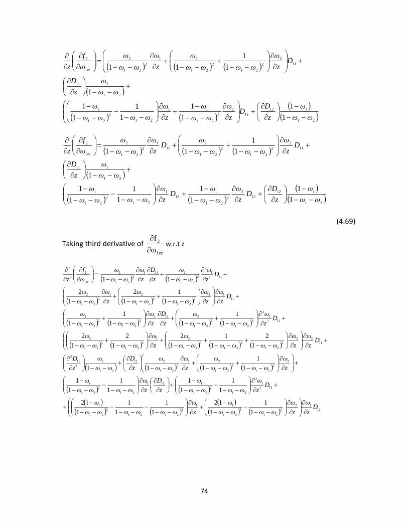
74
21
112
12
2
2
21
11
21
2
21
1
21
211
11
2
2
21
2
21
21
2
21
2
1
2
1
1
1
1
1
1
1
1
1
1
1
11
ωω
ω
z
DD
z
ω
ωω
ω
z
ω
ωωωω
ω
ωω
ω
z
D
Dz
ω
ωωωω
ω
z
ω
ωω
ω
ω
f
zzz
21
112
12
2
2
21
1
12
1
21
2
21
1
21
211
11
2
2
21
2
21
2
11
1
2
21
2
1
2
1
1
1
1
1
1
1
1
1
1
1
11
ωω
ω
z
DD
z
ω
ωω
ωD
z
ω
ωωωω
ω
ωω
ω
z
D
Dz
ω
ωωωω
ωD
z
ω
ωω
ω
ω
f
zzz
(4.69)
Taking third derivative of 1zz
2
ω
f
w.r.t z
12
12
2
21
3
21
11
2
2121
3
21
1
122
1
2
21
2
21
1121
21
2
21
1
2
2
21
2
21
21
2
21
211
21
2
2
11
2
11
22
3
21
2
21
3
21
21
3
21
3
21
2
112
2
2
2
21
2
21
2112
2
21
2
21
2
11
12
2
21
3
21
21
3
21
2
112
1
2
2
21
2111
2
21
2
1
2
2
2
1
1
1
12
1
1
1
1
1
12
1
1
1
1
1
1
1
1
1
1
111
1
2
1
1
1
2
1
2
1
2
1
1
11
1
1
1
1
1
2
1
2
11
Dz
ω
z
ω
ωωωω
ω
z
ω
ωωωωωω
ω
Dz
ω
ωωωω
ω
z
D
z
ω
ωωωω
ω
z
ω
ωωωω
ω
z
ω
ωω
ω
z
D
ωω
ω
z
D
Dz
ω
z
ω
ωωωωωω
ω
z
ω
ωωωω
ω
Dz
ω
ωωωω
ω
z
D
z
ω
ωωωω
ω
Dz
ω
z
ω
ωωωω
ω
z
ω
ωω
ω
Dz
ω
ωω
ω
z
D
z
ω
ωω
ω
ω
f
zzz

75
z
D
zzz
D
Dz
z
zD
zz
D
z
122
2
21
11
21
2
21
1
21
1
2
12
2
12
2
2
3
21
1
1
2
21
3
21
1
122
2
2
2
21
1122
2
21
1
1
1
1
1
1
1
1
1
1
12
1
1
1
12
1
1
1
1
(4.70)
The variational derivatives of 1f and 2f , Equations (4.51-4.54) are given below
11
2
1
2
21
2
21
21
2
21
2
2
1
2
21
2
111
11
1
1
1
1
1
1
1
1
1
1
δD
z
ω
ωω
ω
z
ω
z
ω
ωωωω
ω
z
ω
ωω
ω
λδDD
fλ
(4.71)
122
2
21
2
21
2
21
2
21
2
112
12
1
1
1
1
1
1
1
1
δD
z
ω
ωωωω
ω
z
ω
z
ω
ωω
ω
λδDD
fλ
(4.72)
21
2
2
2
21
2
2
1
2
21
1
12
2
21
1
2
1
21
2
21
1
121
21
1
1
1
1
1
1
1
1
1
δD
z
ω
ωω
ω
z
ω
ωω
ω
z
ω
z
ω
ωω
ω
z
ω
ωωωω
ω
λδDD
fλ
(4.73)
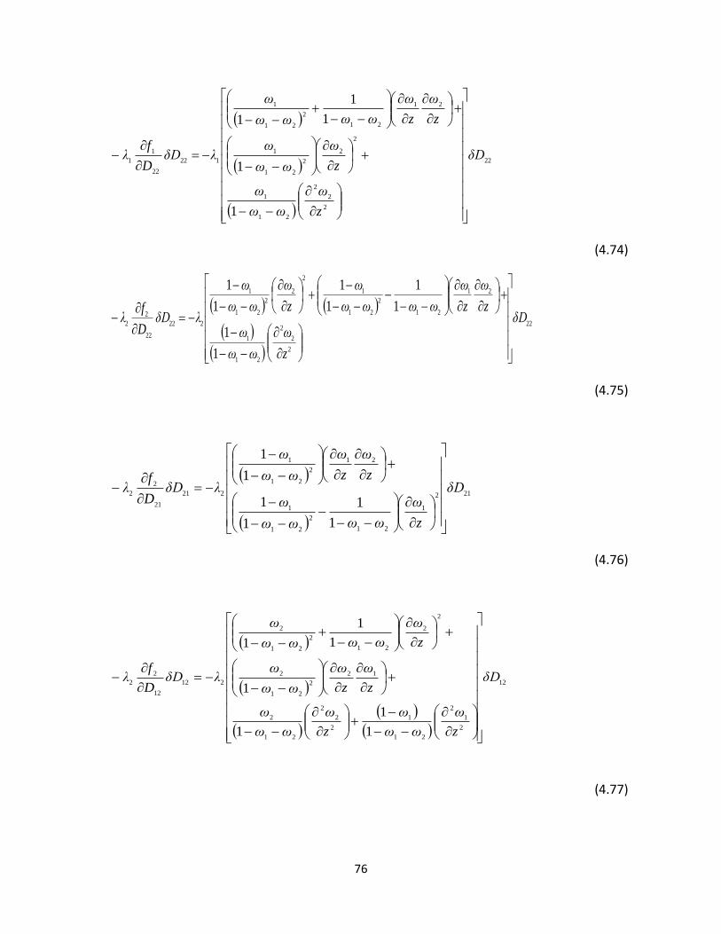
76
22
2
2
2
21
1
2
2
2
21
1
21
21
2
21
1
122
22
1
1
1
1
1
1
1
δD
z
ω
ωω
ω
z
ω
ωω
ω
z
ω
z
ω
ωωωω
ω
λδDD
fλ
(4.74)
22
2
2
2
21
1
21
21
2
21
1
2
2
2
21
1
222
22
2
2
1
1
1
1
1
1
1
1
δD
z
ω
ωω
ω
z
ω
z
ω
ωωωω
ω
z
ω
ωω
ω
λδDD
fλ
(4.75)
212
1
21
2
21
1
21
2
21
1
221
21
2
2
1
1
1
1
1
1
δD
z
ω
ωωωω
ω
z
ω
z
ω
ωω
ω
λδDD
fλ
(4.76)
12
2
1
2
21
1
2
2
2
21
2
12
2
21
2
2
2
21
2
21
2
212
12
2
2
1
1
1
1
1
1
1
δD
z
ω
ωω
ω
z
ω
ωω
ω
z
ω
z
ω
ωω
ω
z
ω
ωωωω
ω
λδDD
fλ
(4.77)

77
11
2
1
2
21
2
2
1
2
21
2
21
21
2
21
2
211
11
2
2
1
1
1
1
1
δD
z
ω
ωω
ω
z
ω
ωω
ω
z
ω
z
ω
ωωωω
ω
λδDD
fλ
(4.78)
4.6 Computational Algorithm
Based on the necessary conditions for the minimum of the objective functional, the
following computational algorithm was developed to determine the concentration-
dependent, multi-component diffusion coefficients.
1 Step A: Initialize and . Four initial estimates of diffusivities, i.e.
and , were provided to initialize the program.
2 Step B: Simultaneously integrate the state equations (model) subject to the initial and
boundary conditions, to obtain the values of for each node. To implement the
numerical solution, the state equations were expressed in finite-difference form along z
direction. The model of the diffusion cell was divided into equal-spaced grid points in the z
direction. In this way, each state equation was transformed into a set of simultaneous
ordinary differential equations. The fifth-order, adaptive-step method of Runge-Kutta-

78
Fehlberg was used with Cash-Karp parameters to achieve an accurate solution with
minimum computational effort. The values of state variables( and ), at
each grid point in the space of t and z are saved.
3 Step D: Evaluate the objective functional.
4 If there is no difference between the calculated mass and the experimental mass of the
gases absorbed then STOP, otherwise go the next step.
5 Step E: Integrate the costate equations backward, subject to the final boundary conditions,
using stored values of to get the values of
at each grid point. The
costate equations must be solved backward in the time domain. Since they are dependent
on concentration, they can be only solved after solving the state equation in the forward
direction in the time domain. The solution of these equations provides the variational
derivatives to be used in the next step.
6 Step F: Improve using the gradient correction.
7 Obtain the new and improved values of at each grid point in the time interval
using the variational derivative as follows:
where
and is a small positive number whose optimal
value provides maximum reduction in the objective functional.
Using , repeat the computations Step 2 onward until there is no further improvement
in the objective functional. When the improvement is negligible, the values are optimal.
79
The variational derivatives were used in conjunction with the Broyden–Fletcher–Goldfarb–
Shanno algorithm (BFGS) method to improve the diffusivities. The optimal control
algorithm was programmed in C++. Figure 4.2 shows the computational algorithm.
The architecture of the computer program that was used to estimate optimal values of
concentration dependent multi-component diffusivities is shown in Figure 4.3. The
computer program is divided in five main Blocks, namely: A, B, C, D and E. We will discuss
these Blocks briefly. Block A includes the main file of the program that consists of Broyden–
Fletcher–Goldfarb–Shanno algorithm (BFGS) and model class. The BFGS is gradient
improvement method. Model class solves the mathematical model. Model class is
connected to the Block B that contains the mass transfer model, experimental results and
the input file that contains various information incluing diffusivity guesses, number of grid
points, step size, tolerance, molecular weight of the polymer, polymer density etc.
When the program executes, the model class solves the differential equations i.e. state
equations (in forwards direction) in Block B using fifth-order adaptive-step method of
Runge-Kutta-Fehlberg with Cash-Karp parameters method and the information in the input
file. Once the differential equations are solved, the programme calculates the difference
between the calculated gas mass absorbed and the experimental gas mass absorbed in
Block C using composite Simpson 1/3 and Simpson 1/8 integration rule.
Next, the program solves the costate equations (in backward direction), in Block B, using
Runge-Kutta-Fehlberg fifth order method and the results obtained by solving the state
equation previously.
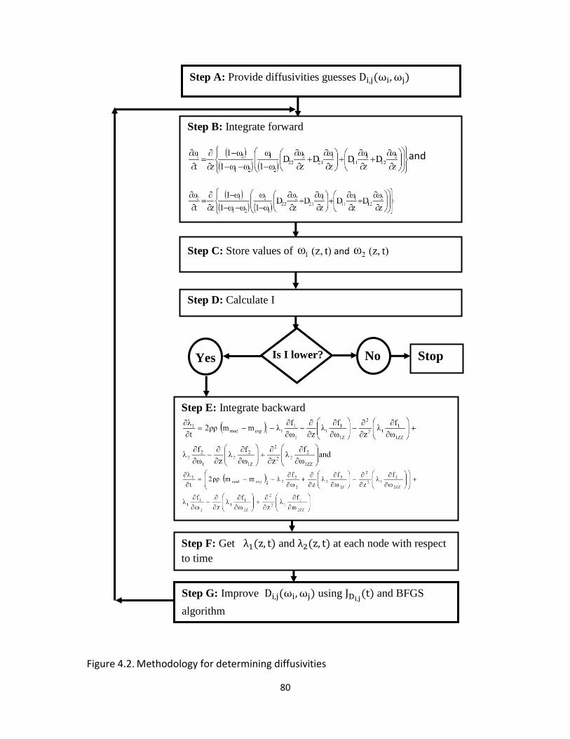
80
Figure 4.2. Methodology for determining diffusivities
Step A: Provide diffusivities guesses ω ω
Step B: Integrate forward
and
Step C: Store values of and
Step D: Calculate I
Step E: Integrate backward
Step F: Get λ z t and λ z t at each node with respect
to time
Step G: Improve ω ω using j t and BFGS
algorithm
Stop No Is I lower? Yes
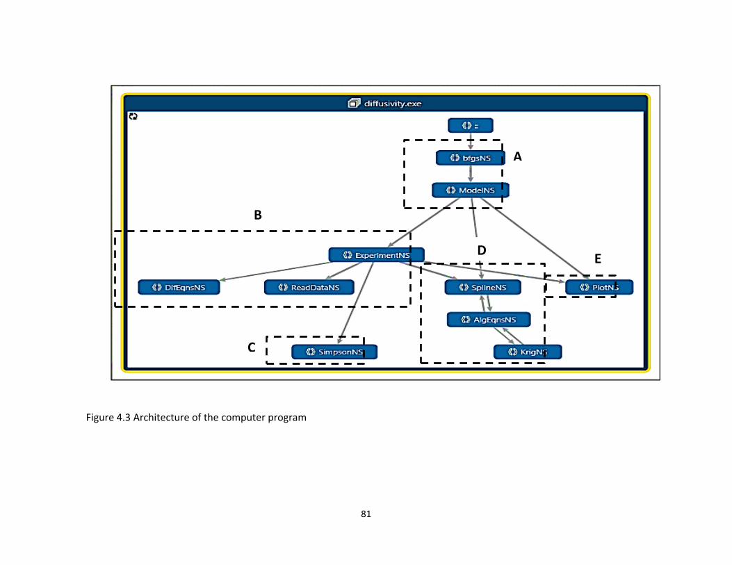
81
Figure 4.3 Architecture of the computer program
A
B
C
D E

82
Based on the difference between the calculated gas mass absorbed and the experimental
gas mass absorbed the program makes the use of variational derivatives and modify the
diffusivity estimate using Krig in Block D. Krig is a 3D interpolation method.
The BFGS uses all the above information via model class and minimizes the difference
between the calculated gas mass absorbed and the experimental gas mass absorbed. The
results are printed in Block E.
The above process continues until difference between the calculated gas mass absorbed
and the experimental gas mass absorbed is minimum. The C++ codes for calculating
variational derivatives and the improvement in the diffusivity values are given in appendix
C. The results obtained in this study are presented in the next chapter.

83
5 RESULTS and DISCUSSION
Since this work is a first step towards developing an optimal control framework to
determine concentration dependent multi-component diffusivities so we decided to work
at room temperature (23oC) and a pressure of 224 kPa. Using the aforementioned
experiments and calculations, we determined the concentration-dependent multi-
component diffusivities and solubility of nitrogen and carbon dioxide in polystyrene. The
algorithm developed in Chapter 3 was used to determine the concentration-dependent,
multi-component diffusivities. The parameters used in the calculations are provided in
Table 5.1
Table 5.1 Parameters used in calculating diffusivities
Parameters Value
Mass of polymer
Density of the polymer Diameter of the polymer sample Thickness of the polymer sample Number of vs. points 10
Number of grid points along the z direction
10 and 15
To arrive at the optimal diffusivities we provided different diffusivities guesses, the
computer program was run and the improvement in the objective functional, and the
concentration dependant diffusivities obtained were recorded. Approximately, hundreds of
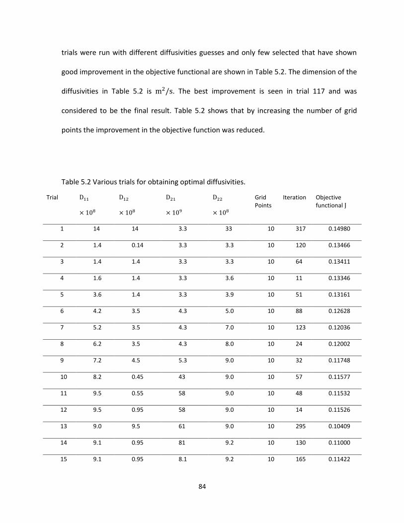
84
trials were run with different diffusivities guesses and only few selected that have shown
good improvement in the objective functional are shown in Table 5.2. The dimension of the
diffusivities in Table 5.2 is . The best improvement is seen in trial 117 and was
considered to be the final result. Table 5.2 shows that by increasing the number of grid
points the improvement in the objective function was reduced.
Table 5.2 Various trials for obtaining optimal diffusivities.
Trial
Grid Points
Iteration Objective functional
1 14 14 3.3 33 10 317 0.14980
2 1.4 0.14 3.3 3.3 10 120 0.13466
3 1.4 1.4 3.3 3.3 10 64 0.13411
4 1.6 1.4 3.3 3.6 10 11 0.13346
5 3.6 1.4 3.3 3.9 10 51 0.13161
6 4.2 3.5 4.3 5.0 10 88 0.12628
7 5.2 3.5 4.3 7.0 10 123 0.12036
8 6.2 3.5 4.3 8.0 10 24 0.12002
9 7.2 4.5 5.3 9.0 10 32 0.11748
10 8.2 0.45 43 9.0 10 57 0.11577
11 9.5 0.55 58 9.0 10 48 0.11532
12 9.5 0.95 58 9.0 10 14 0.11526
13 9.0 9.5 61 9.0 10 295 0.10409
14 9.1 0.95 81 9.2 10 130 0.11000
15 9.1 0.95 8.1 9.2 10 165 0.11422
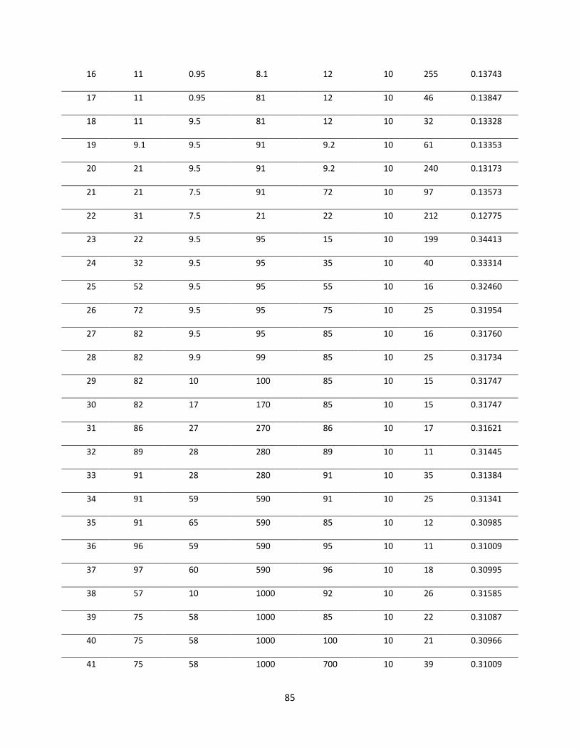
85
16 11 0.95 8.1 12 10 255 0.13743
17 11 0.95 81 12 10 46 0.13847
18 11 9.5 81 12 10 32 0.13328
19 9.1 9.5 91 9.2 10 61 0.13353
20 21 9.5 91 9.2 10 240 0.13173
21 21 7.5 91 72 10 97 0.13573
22 31 7.5 21 22 10 212 0.12775
23 22 9.5 95 15 10 199 0.34413
24 32 9.5 95 35 10 40 0.33314
25 52 9.5 95 55 10 16 0.32460
26 72 9.5 95 75 10 25 0.31954
27 82 9.5 95 85 10 16 0.31760
28 82 9.9 99 85 10 25 0.31734
29 82 10 100 85 10 15 0.31747
30 82 17 170 85 10 15 0.31747
31 86 27 270 86 10 17 0.31621
32 89 28 280 89 10 11 0.31445
33 91 28 280 91 10 35 0.31384
34 91 59 590 91 10 25 0.31341
35 91 65 590 85 10 12 0.30985
36 96 59 590 95 10 11 0.31009
37 97 60 590 96 10 18 0.30995
38 57 10 1000 92 10 26 0.31585
39 75 58 1000 85 10 22 0.31087
40 75 58 1000 100 10 21 0.30966
41 75 58 1000 700 10 39 0.31009

86
42 10 1 10 60 10 26 0.11350
43 0.15 0.15 1.5 0.15 10 56 1.43297
44 0.17 0.17 1.7 0.17 10 53 1.42830
45 0.19 0.19 1.9 0.19 10 50 1.42304
46 0.23 0.23 2.3 0.23 10 41 1.41158
47 0.35 0.35 3.5 0.35 10 56 1.37661
48 0.37 0.37 3.7 0.37 10 65 1.37104
49 0.3 0.3 3 0.3 10 47 1.39092
50 0.4 0.4 4 0.4 10 73 1.36286
51 0.1 0.4 4 0.63 10 13 0.83190
52 1 0.4 4 8.3 10 17 1.23294
53 3.3 0.4 4 0.13 10 8 0.92094
54 0.33 0.4 4 0.93 10 73 1.36286
55 0.43 0.4 4 0.83 10 50 1.42304
56 0.53 0.4 4 1 10 73 1.36286
57 0.83 0.4 4 3.3 10 50 1.42304
58 9.3 0.4 4 0.63 10 56 1.37661
59 14 14 3.3 33 15 288 0.15513
60 1.4 0.14 3.3 3.3 15 102 0.13510
61 1.4 1.4 3.3 3.3 15 52 0.10141
62 1.6 1.4 3.3 3.6 15 6 0.13106
63 3.6 1.4 3.3 3.9 15 44 0.13214
64 4.2 3.5 4.3 5.0 15 79 0.13117
65 5.2 3.5 4.3 7.0 15 111 0.13112
66 6.2 3.5 4.3 8.0 15 13 0.12115
67 7.2 4.5 5.3 9.0 15 27 0.11887
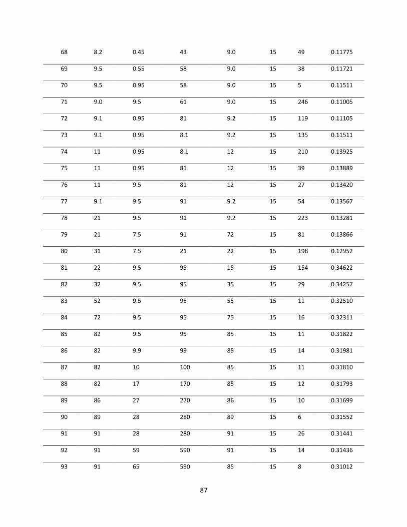
87
68 8.2 0.45 43 9.0 15 49 0.11775
69 9.5 0.55 58 9.0 15 38 0.11721
70 9.5 0.95 58 9.0 15 5 0.11511
71 9.0 9.5 61 9.0 15 246 0.11005
72 9.1 0.95 81 9.2 15 119 0.11105
73 9.1 0.95 8.1 9.2 15 135 0.11511
74 11 0.95 8.1 12 15 210 0.13925
75 11 0.95 81 12 15 39 0.13889
76 11 9.5 81 12 15 27 0.13420
77 9.1 9.5 91 9.2 15 54 0.13567
78 21 9.5 91 9.2 15 223 0.13281
79 21 7.5 91 72 15 81 0.13866
80 31 7.5 21 22 15 198 0.12952
81 22 9.5 95 15 15 154 0.34622
82 32 9.5 95 35 15 29 0.34257
83 52 9.5 95 55 15 11 0.32510
84 72 9.5 95 75 15 16 0.32311
85 82 9.5 95 85 15 11 0.31822
86 82 9.9 99 85 15 14 0.31981
87 82 10 100 85 15 11 0.31810
88 82 17 170 85 15 12 0.31793
89 86 27 270 86 15 10 0.31699
90 89 28 280 89 15 6 0.31552
91 91 28 280 91 15 26 0.31441
92 91 59 590 91 15 14 0.31436
93 91 65 590 85 15 8 0.31012
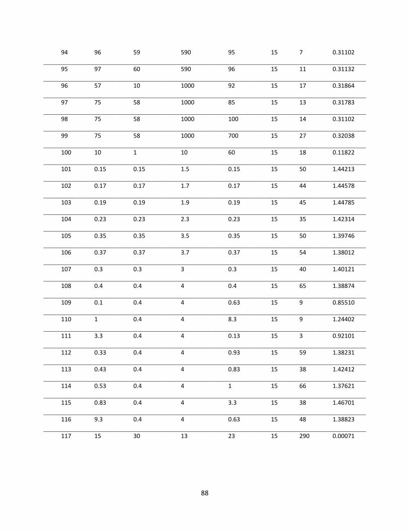
88
94 96 59 590 95 15 7 0.31102
95 97 60 590 96 15 11 0.31132
96 57 10 1000 92 15 17 0.31864
97 75 58 1000 85 15 13 0.31783
98 75 58 1000 100 15 14 0.31102
99 75 58 1000 700 15 27 0.32038
100 10 1 10 60 15 18 0.11822
101 0.15 0.15 1.5 0.15 15 50 1.44213
102 0.17 0.17 1.7 0.17 15 44 1.44578
103 0.19 0.19 1.9 0.19 15 45 1.44785
104 0.23 0.23 2.3 0.23 15 35 1.42314
105 0.35 0.35 3.5 0.35 15 50 1.39746
106 0.37 0.37 3.7 0.37 15 54 1.38012
107 0.3 0.3 3 0.3 15 40 1.40121
108 0.4 0.4 4 0.4 15 65 1.38874
109 0.1 0.4 4 0.63 15 9 0.85510
110 1 0.4 4 8.3 15 9 1.24402
111 3.3 0.4 4 0.13 15 3 0.92101
112 0.33 0.4 4 0.93 15 59 1.38231
113 0.43 0.4 4 0.83 15 38 1.42412
114 0.53 0.4 4 1 15 66 1.37621
115 0.83 0.4 4 3.3 15 38 1.46701
116 9.3 0.4 4 0.63 15 48 1.38823
117 15 30 13 23 15 290 0.00071
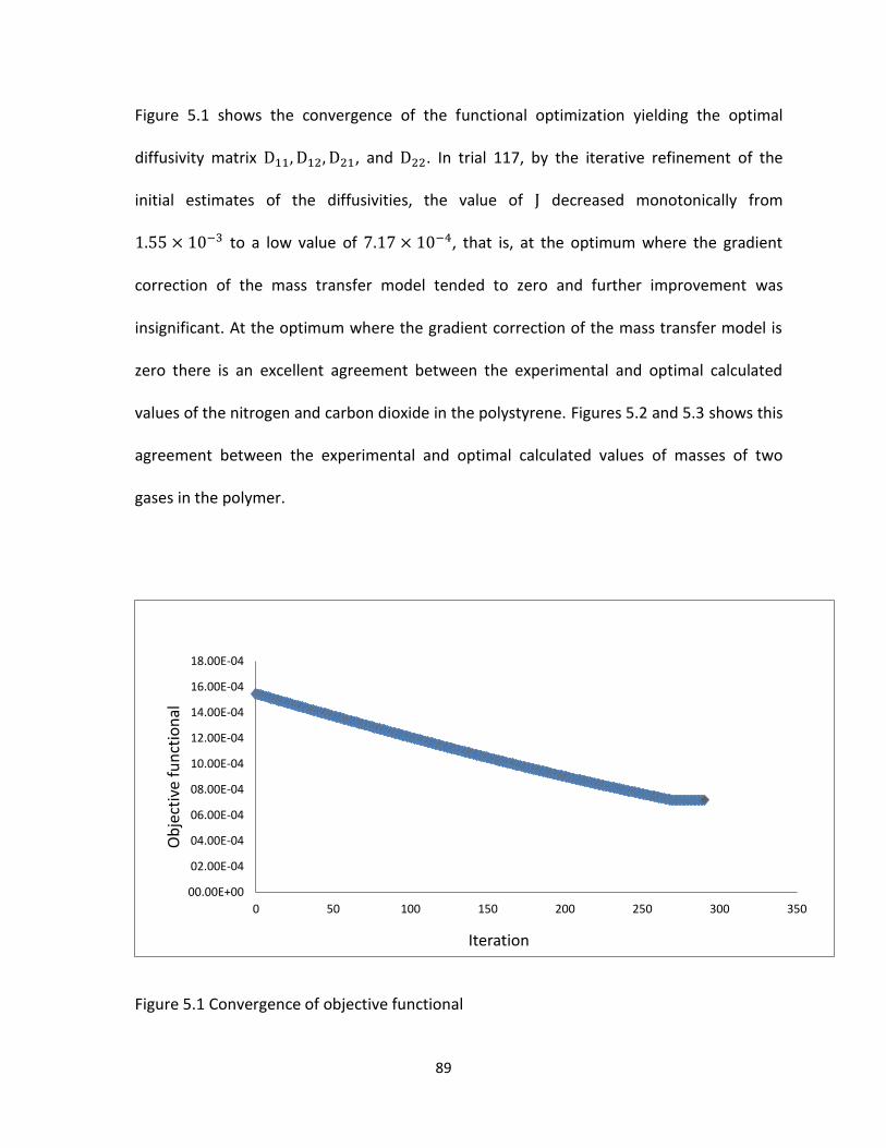
89
Figure 5.1 shows the convergence of the functional optimization yielding the optimal
diffusivity matrix , and . In trial 117, by the iterative refinement of the
initial estimates of the diffusivities, the value of decreased monotonically from
to a low value of , that is, at the optimum where the gradient
correction of the mass transfer model tended to zero and further improvement was
insignificant. At the optimum where the gradient correction of the mass transfer model is
zero there is an excellent agreement between the experimental and optimal calculated
values of the nitrogen and carbon dioxide in the polystyrene. Figures 5.2 and 5.3 shows this
agreement between the experimental and optimal calculated values of masses of two
gases in the polymer.
Figure 5.1 Convergence of objective functional
00.00E+00
02.00E-04
04.00E-04
06.00E-04
08.00E-04
10.00E-04
12.00E-04
14.00E-04
16.00E-04
18.00E-04
0 50 100 150 200 250 300 350
Ob
ject
ive
fun
ctio
nal
Iteration
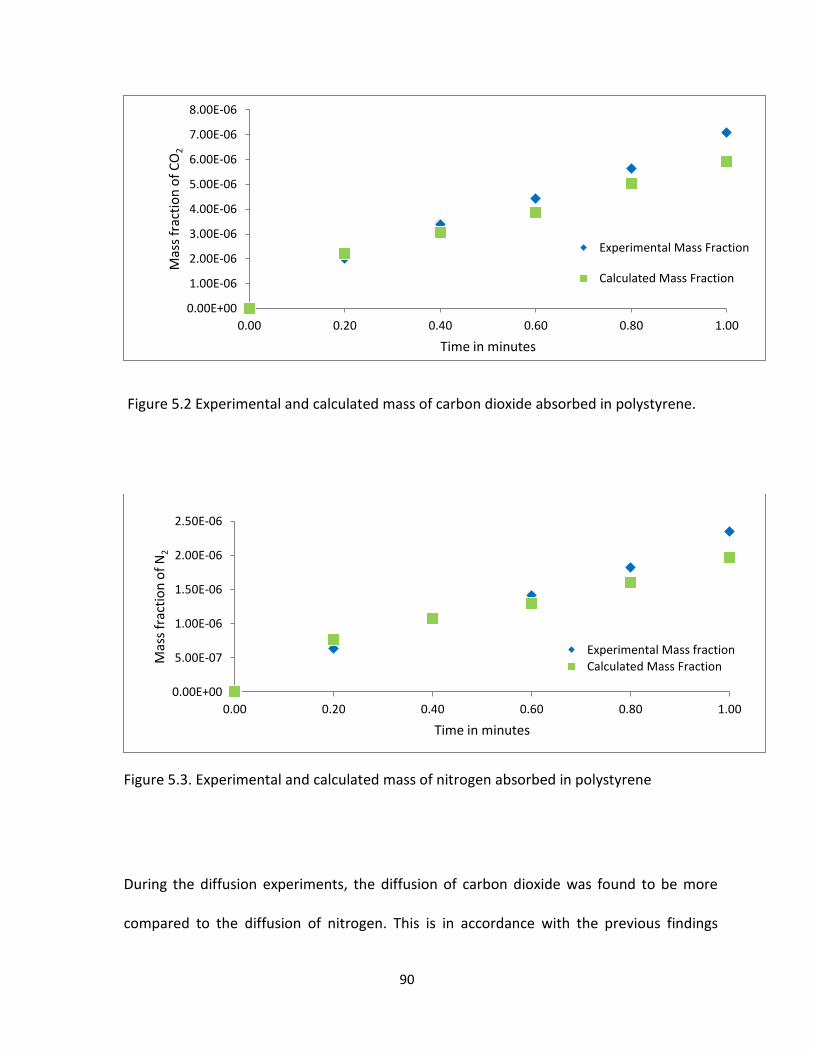
90
Figure 5.2 Experimental and calculated mass of carbon dioxide absorbed in polystyrene.
Figure 5.3. Experimental and calculated mass of nitrogen absorbed in polystyrene
During the diffusion experiments, the diffusion of carbon dioxide was found to be more
compared to the diffusion of nitrogen. This is in accordance with the previous findings
0.00E+00
1.00E-06
2.00E-06
3.00E-06
4.00E-06
5.00E-06
6.00E-06
7.00E-06
8.00E-06
0.00 0.20 0.40 0.60 0.80 1.00
Mas
s fr
acti
on
of
CO
2
Time in minutes
Experimental Mass Fraction
Calculated Mass Fraction
0.00E+00
5.00E-07
1.00E-06
1.50E-06
2.00E-06
2.50E-06
0.00 0.20 0.40 0.60 0.80 1.00
Mas
s fr
acti
on
of
N2
Time in minutes
Experimental Mass fraction
Calculated Mass Fraction
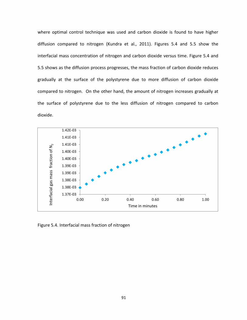
91
where optimal control technique was used and carbon dioxide is found to have higher
diffusion compared to nitrogen (Kundra et al., 2011). Figures 5.4 and 5.5 show the
interfacial mass concentration of nitrogen and carbon dioxide versus time. Figure 5.4 and
5.5 shows as the diffusion process progresses, the mass fraction of carbon dioxide reduces
gradually at the surface of the polystyrene due to more diffusion of carbon dioxide
compared to nitrogen. On the other hand, the amount of nitrogen increases gradually at
the surface of polystyrene due to the less diffusion of nitrogen compared to carbon
dioxide.
Figure 5.4. Interfacial mass fraction of nitrogen
1.37E-03
1.38E-03
1.38E-03
1.39E-03
1.39E-03
1.40E-03
1.40E-03
1.41E-03
1.41E-03
1.42E-03
0.00 0.20 0.40 0.60 0.80 1.00
Inte
rfac
ial g
as m
ass
fra
ctio
n o
f N
2
Time in minutes
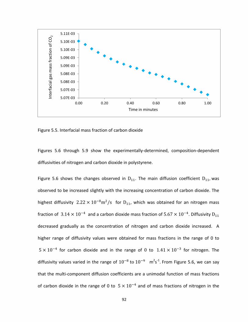
92
Figure 5.5. Interfacial mass fraction of carbon dioxide
Figures 5.6 through 5.9 show the experimentally-determined, composition-dependent
diffusivities of nitrogen and carbon dioxide in polystyrene.
Figure 5.6 shows the changes observed in . The main diffusion coefficient was
observed to be increased slightly with the increasing concentration of carbon dioxide. The
highest diffusivity for , which was obtained for an nitrogen mass
fraction of and a carbon dioxide mass fraction of . Diffusivity
decreased gradually as the concentration of nitrogen and carbon dioxide increased. A
higher range of diffusivity values were obtained for mass fractions in the range of 0 to
for carbon dioxide and in the range of to for nitrogen. The
diffusivity values varied in the range of t m2s-1. From Figure 5.6, we can say
that the multi-component diffusion coefficients are a unimodal function of mass fractions
of carbon dioxide in the range of 0 to and of mass fractions of nitrogen in the
5.07E-03
5.07E-03
5.08E-03
5.08E-03
5.09E-03
5.09E-03
5.10E-03
5.10E-03
5.11E-03
0.00 0.20 0.40 0.60 0.80 1.00
Inte
rfac
ial g
as m
ass
frac
tio
n o
f C
O2
Time in minutes
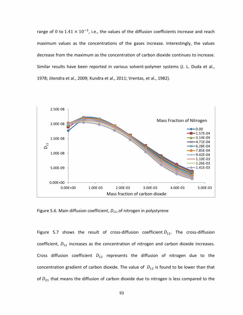
93
range of to , i.e., the values of the diffusion coefficients increase and reach
maximum values as the concentrations of the gases increase. Interestingly, the values
decrease from the maximum as the concentration of carbon dioxide continues to increase.
Similar results have been reported in various solvent-polymer systems (J. L. Duda et al.,
1978; Jitendra et al., 2009; Kundra et al., 2011; Vrentas, et al., 1982).
Figure 5.6. Main diffusion coefficient, D11, of nitrogen in polystyrene
Figure 5.7 shows the result of cross-diffusion coefficient . The cross-diffusion
coefficient, increases as the concentration of nitrogen and carbon dioxide increases.
Cross diffusion coefficient represents the diffusion of nitrogen due to the
concentration gradient of carbon dioxide. The value of is found to be lower than that
of that means the diffusion of carbon dioxide due to nitrogen is less compared to the
0.00E+00
5.00E-09
1.00E-08
1.50E-08
2.00E-08
2.50E-08
0.00E+00 1.00E-03 2.00E-03 3.00E-03 4.00E-03 5.00E-03
D1
1
Mass fraction of carbon dioxde
0.001.57E-043.14E-044.71E-046.28E-047.85E-049.42E-041.10E-031.26E-031.41E-03
Mass Fraction of Nitrogen
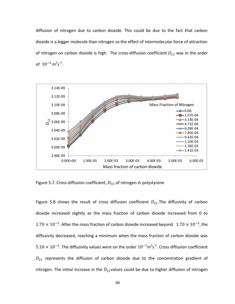
94
diffusion of nitrogen due to carbon dioxide. This could be due to the fact that carbon
dioxide is a bigger molecule than nitrogen so the effect of intermolecular force of attraction
of nitrogen on carbon dioxide is high. The cross-diffusion coefficient was in the order
of m2s-1.
Figure 5.7. Cross-diffusion coefficient, D12, of nitrogen in polystyrene
Figure 5.8 shows the result of cross diffusion coefficient .The diffusivity of carbon
dioxide increased slightly as the mass fraction of carbon dioxide increased from 0 to
. After the mass fraction of carbon dioxide increased beyond , the
diffusivity decreased, reaching a minimum when the mass fraction of carbon dioxide was
. The diffusivity values were on the order m2s-1. Cross diffusion coefficient
represents the diffusion of carbon dioxide due to the concentration gradient of
nitrogen. The initial increase in the values could be due to higher diffusion of nitrogen
2.98E-09
3.00E-09
3.02E-09
3.04E-09
3.06E-09
3.08E-09
3.10E-09
3.12E-09
3.14E-09
0.00E+00 1.00E-03 2.00E-03 3.00E-03 4.00E-03 5.00E-03 6.00E-03
D1
2
Mass fraction of carbon dioxide
0.001.57E-043.14E-044.71E-046.28E-047.85E-049.42E-041.10E-031.26E-031.41E-03
Mass Fraction of Nitrogen

95
due to the concentration gradient of carbon dioxide. Since there is lots of empty spaces
available in the polymer matrix initially, the diffusivity value of is higher. Once the
space in the polymer matrix is saturated with the two gases the effect of nitrogen on
carbon dioxide decreases resulting in the lower values of (Jitendra et al., 2009; Kundra
et al., 2011).
Figure 5.8. Cross-diffusion coefficient, D21, of carbon dioxide in polystyrene
Figure 5.9 shows that the main diffusion coefficient, which increases as the
concentrations of nitrogen and carbon dioxide increases.
The main diffusion coefficient remained high with low concentrations of carbon
dioxide. The diffusivity was found to be on the order of m2s-1 .The above results are in
accordance with the findings of Biesenberger, 1983, who reported concentration-
dependant diffusion coefficients of ethyl benzene in molten polystyrene and found that a
1.2996E-07
1.2998E-07
1.3000E-07
1.3002E-07
1.3004E-07
1.3006E-07
1.3008E-07
1.3010E-07
1.3012E-07
1.3014E-07
1.3016E-07
0.00E+00 1.00E-03 2.00E-03 3.00E-03 4.00E-03 5.00E-03 6.00E-03
D2
1
Mass fraction of carbon dioxide
0.001.57E-043.14E-044.71E-046.28E-047.85E-049.42E-041.10E-031.26E-031.41E-03
Mass Fraction of Nitrogen
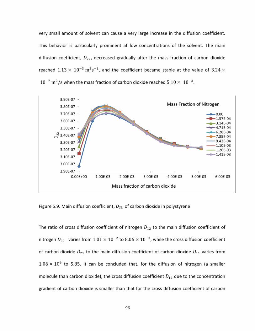
96
very small amount of solvent can cause a very large increase in the diffusion coefficient.
This behavior is particularly prominent at low concentrations of the solvent. The main
diffusion coefficient, decreased gradually after the mass fraction of carbon dioxide
reached , and the coefficient became stable at the value of
when the mass fraction of carbon dioxide reached .
Figure 5.9. Main diffusion coefficient, D22, of carbon dioxide in polystyrene
The ratio of cross diffusion coefficient of nitrogen to the main diffusion coefficient of
nitrogen varies from to , while the cross diffusion coefficient
of carbon dioxide to the main diffusion coefficient of carbon dioxide varies from
to . It can be concluded that, for the diffusion of nitrogen (a smaller
molecule than carbon dioxide), the cross diffusion coefficient due to the concentration
gradient of carbon dioxide is smaller than that for the cross diffusion coefficient of carbon
2.90E-07
3.00E-07
3.10E-07
3.20E-07
3.30E-07
3.40E-07
3.50E-07
3.60E-07
3.70E-07
3.80E-07
3.90E-07
0.00E+00 1.00E-03 2.00E-03 3.00E-03 4.00E-03 5.00E-03 6.00E-03
D2
2
Mass fraction of carbon dioxide
0.001.57E-043.14E-044.71E-046.28E-047.85E-049.42E-041.10E-031.26E-031.41E-03
Mass Fraction of Nitrogen
97
dioxide (a larger molecule) due to the concentration gradient of nitrogen (a smaller
molecule), as shown in Figures 5.10 and 5.11. Our findings are in accordance with the
findings of E. L. Cussler & Breuer, 1972, where acetone a smaller molecule, dragged the
bigger molecule, sodium sulfate, and resulted in increased diffusion of sodium sulfate
(bigger molecule).
But these results are in contrast to the findings of Lin et al., 2009, they found that the
diffusion of di-ethanol amine (a smaller molecule, compared to methyl di-ethanol amine),
the cross-diffusion effect ( ) due to the concentration gradient of methyl di-ethanol
amine is larger than that for the diffusion of methyl di-ethanol amine (a larger molecule)
(D21) due to the concentration gradient of di-ethanol amine (a smaller molecule).
Since multi-component diffusion is a complex process, further study is needed on the effect
of molecular size, polarity, kinetic energy of molecules, dipole moment, density, viscosity,
temperature, and pressure on multi-component diffusion.
In general, the diffusivity of carbon dioxide in polystyrene was found to be greater than
that of nitrogen, which was in accordance with the findings of other researchers who used
carbon dioxide and nitrogen separately in polypropylene and LDPE systems (Jitendra et al.,
2009; Kundra et al., 2011).

98
Figure 5.10. Ratio of cross diffusion coefficient (D21/D11) of carbon dioxide due to the concentration gradient of nitrogen
Figure 5.11. Ratio of cross diffusion coefficient (D12/D22) of nitrogen due to the concentration gradient of carbon dioxide
0.00E+00
2.00E+01
4.00E+01
6.00E+01
8.00E+01
1.00E+02
1.20E+02
0.00E+00 1.00E-03 2.00E-03 3.00E-03 4.00E-03 5.00E-03
D2
1/D
11
Mass fraction of carbon dioxide
7.80E-03
8.30E-03
8.80E-03
9.30E-03
9.80E-03
1.03E-02
0.00E+00 1.00E-03 2.00E-03 3.00E-03 4.00E-03 5.00E-03
D1
2/D
22
Mass fraction of carbon dioxide
Series2Series3Series4Series5Series6Series7Series8Series9Series10
Mass Fraction of Nitrogen
Mass Fraction of Nitrogen
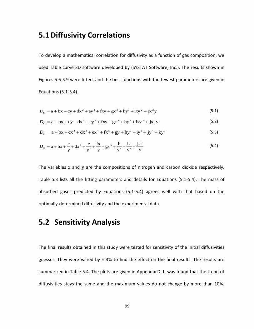
99
5.1 Diffusivity Correlations
To develop a mathematical correlation for diffusivity as a function of gas composition, we
used Table curve 3D software developed by (SYSTAT Software, Inc.). The results shown in
Figures 5.6-5.9 were fitted, and the best functions with the fewest parameters are given in
Equations (5.1-5.4).
yjxixyhygxfxyeydxcybxa 223322
11D (5.1)
yjxixyhygxfxyeydxcybxa 223322
12D (5.2)
54325432
21kyjyiyhygyfxexdxcxbxa D (5.3)
y
jx
y
ix
y
hgx
y
fx
y
edx
y
cbxa
2
23
3
2
2
22D (5.4)
The variables and are the compositions of nitrogen and carbon dioxide respectively.
Table 5.3 lists all the fitting parameters and details for Equations (5.1-5.4). The mass of
absorbed gases predicted by Equations (5.1-5.4) agrees well with that based on the
optimally-determined diffusivity and the experimental data.
5.2 Sensitivity Analysis
The final results obtained in this study were tested for sensitivity of the initial diffusivities
guesses. They were varied by ± 3% to find the effect on the final results. The results are
summarized in Table 5.4. The plots are given in Appendix D. It was found that the trend of
diffusivities stays the same and the maximum values do not change by more than 10%.

100
Table 5.3. Parameters for diffusivity correlation at 230C and 224 kPa
Parameter
a
b
c
0
d
e
6.6268 0
f
0
g
h
0
i
0
j
0
k 0 0 8.7533 0
Coefficient of Determination
0.9998 0.9985 0.9907 1
Fit standard error
0
F-statistic 7502.8440 678.5260 951.8373
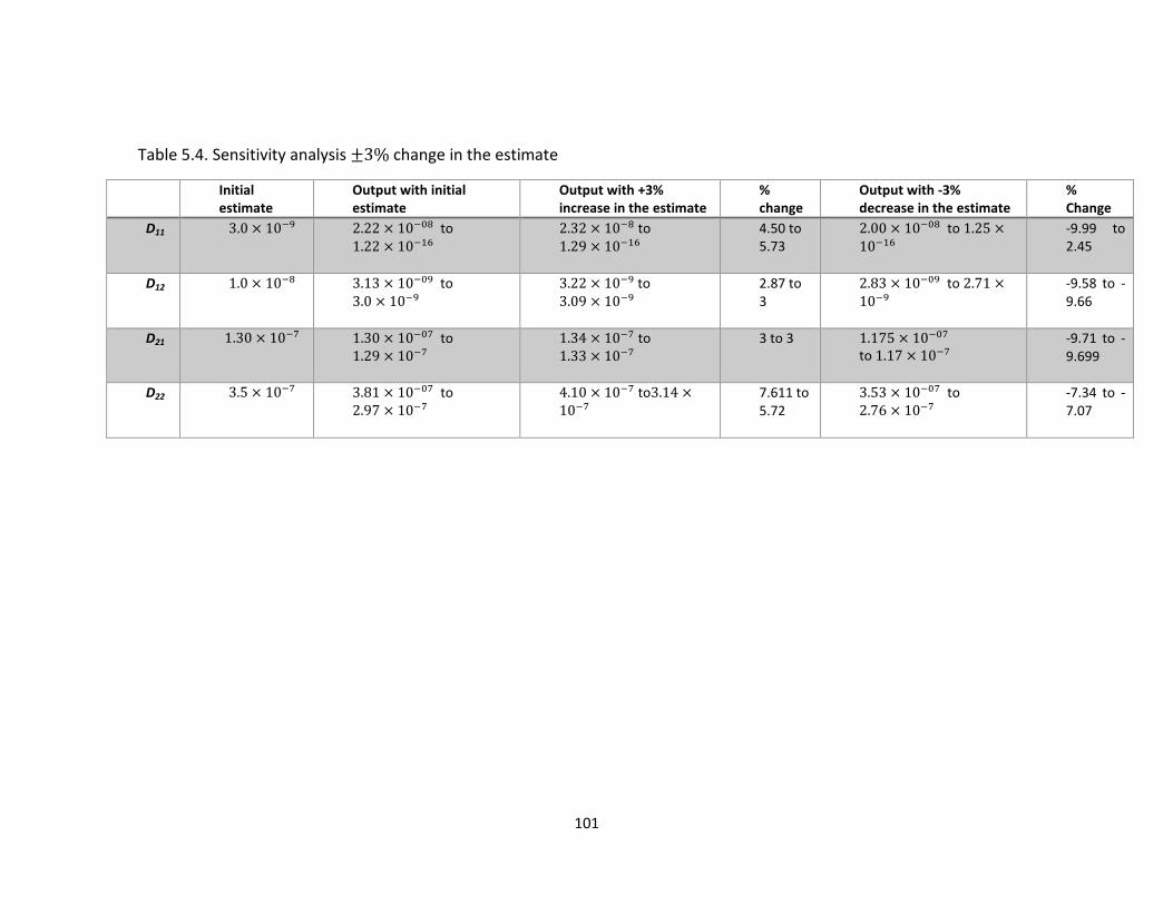
101
Table 5.4. Sensitivity analysis change in the estimate
Initial estimate
Output with initial estimate
Output with +3% increase in the estimate
% change
Output with -3% decrease in the estimate
% Change
D11 to
to
4.50 to 5.73
to
-9.99 to 2.45
D12 to
to
2.87 to 3
to
-9.58 to -9.66
D21 to
to
3 to 3
to
-9.71 to -9.699
D22 to
to
7.611 to 5.72
to
-7.34 to -7.07
102
6 CONCLUSIONS and
RECOMMENDATIONS
6.1 CONCLUSIONS
In this study, we derived a detailed, dynamic, mass-transfer model of the experimental
diffusion process for the polymer phase to provide the temporal masses of gases in the
polymer during the diffusion experiments. Due to the presence of highly non-linear partial
differential equations, the analytical solution to this problem is not possible. Therefore, the
optimal control strategy was used to solve this problem numerically.
For this purpose an optimal control framework was developed to determine
multicomponent concentration dependent diffusivities. Necessary conditions were
determined at which the error between the calculated and experimental gas masses was
minimized. The satisfaction of these conditions determines the unknown diffusivities. Then,
these conditions were used to develop an optimal control frame work.
The above optimal control framework was applied to the ternary system of nitrogen (1)
and carbon dioxide (2) in polystyrene (3) at room temperature (23oC) and a pressure of 224
kPa. Solubility and diffusion experiments data were used along with the detailed mass
103
transfer model and optimal control framework to calculate the multi-component
diffusivities of nitrogen and carbon dioxide in polystyrene as a function of their
compositions. The diffusivity of carbon dioxide was found to be greater than that of
nitrogen. The value of the main diffusion coefficient was found to increase as the
concentration of carbon dioxide increased. The highest value of obtained was
for nitrogen mass fraction of and for a carbon dioxide
mas fraction of . The decreased after the mass fraction carbon dioxide
mass fraction of . The diffusivity varied in the range of t .
The cross-diffusion coefficient increased as the concentrations of nitrogen and carbon
dioxide increased. The diffusivity reached its maximum value when the concentrations of
nitrogen and carbon dioxide were at their maximum values. The diffusivity was of the order
of .
A trend similar to that of was observed with cross-diffusion coefficient . The
diffusivity of carbon dioxide increased for the mass fractions of carbon dioxide ranging
from 0 to . The diffusivity was found to be of the order of . After
the carbon dioxide mass fraction reached , the diffusivity decreased as the
mass of carbon dioxide increased, reaching a minimum at the carbon dioxide mass fraction
of .
The diffusion coefficient, was found to increase with the concentrations of nitrogen
and carbon dioxide. Diffusivity remained high with low concentrations of carbon
dioxide. The diffusivity was found to be of the order of .
104
6.2 RECOMMENDATIONS
This work was a first step towards producing the important, fundamental diffusivity data
that are required for chemical industries. Optimal control framework developed in this
study can be used to generate concentration dependent multicomponent diffusivity data
for two gases and a liquid. Future experiments can be done with different gases and
polymers at different temperatures and pressures.
105
References
Amooghina, A. E., Shehnib, P. M., Ghadimic, A., Sadrzadehc, M., & Mohammadib, T. (2013). Mathematical modeling of mass transfer in multicomponent gas mixture across the synthesized composite polymeric membrane. Journal of Industrial and Engineering Chemistry, 19(3), 870–885.
Arnold, K. R., & Toor, H. L. (1967). Unsteady diffusion in ternary gas mixtures. AICHE Journal, 13(5), 909-914.
Biesenberger, J. A. (1983). Devolatilization of polymers fundamentals of equipment applications. Hanser.
Bouchet, R., & Mevrel, R. (27). Calculating the composition-dependent diffusivity matrix along a diffusion path in ternary systems : Application to β-(ni, pt)al. 2003, 3, 295-303.
Cussler, E. L. (Ed.). (2009). Diffusion, mass transfer in fluid systems (3rd ed.). United Kingdom: Cambridge.
Cussler, E. L., & Lightfoot, E. N. (1965). Multicomponent diffusion involving high polymers. I. diffusion of monodisperse polystyrene in mixed solvents. The Journal of Physical Chemistry, 69(4), 1135.
Cussler, E. L., & Peter, J. D. (1966). An experimental comparison of the gouy and the diaphragm cell methods for studying isothermal ternary diffusion. The Journal of Chemical Physics, 70(6), 1880.
Cussler, E. L., & Breuer, M. M. (1972). Accelerating diffusion with mixed solvents. AICHE Journal, 18(4), 812-816.
Denn, M. M. (1969). Optimization by variational methods McGraw-Hill, New York.
Duda, J. L. (1985). Molecular diffusion in polymeric systems. Pure and Applied Chemistry, 57(11), 1681.
Duda, J. L., Ni, Y. C., & Vrentas, J. S. (1978). Diffusion of ethylbenzene in molten polystyrene. Journal of Applied Polymer Science, 22(3), 689-699.
Felder, R. M., & Huvard, G. S. (1980). Methods in experimental physics. (pp. 315)
Fick, A. (1995). On liquid diffusion . Journal of Membrane Science, Elsevier(100), 33-38.
106
Ghoreyshi, A. A., Farhadpour, F. A., & Soltanieh, M. (2004). A general model for ulticomponent transport in nonporous membranes based on Maxwell-Stefan formulation. hemicalEngineering Communications, 191(4), 460-499.
Graham, T. (1833). On the law of diffusion of gases. Philosophical Magazine, 2(9)
Graham, T. (1850). On the diffusion of liquids. Philosophical Transactions of the Royal Society A, 140, 1-46.
Jitendra, T., Upreti, R. Simant., & Lohi, A. (2009). Experimental determination of oncentration-dependent carbon dioxide diffusivity in LDPE. Journal of Applied Polymer Science, 111(1), 380.
Kirk, D. E. (1970). Optimal control theory, an introduction . New York, USA: Dover Publications.
Kjetil, B., Haugen, & Firoozabadi, A. (2006). On measurement of molecular and thermal diffusion coefficients in multicomponent mixtures. The Journal of Physical Chemistry B, 110(35), 17678-17682.
Krishnamurthy, R., & Taylor, R. (1982). Calculation of multicomponent mass tranfer at high tranfer rates. The Chemical Engineering Journal, 25(1), 47-54.
Kundra, P., Upreti, R., Simant., Ali, L., & Jiangning, W. (2011). Experimental determination of composition-dependent diffusivity of carbon dioxide in polypropylene. Journal of Chemical & Engineering Data, 56(1), 21-26.
Kwag, C., Manke, C. W., & and Gulari, E. (1999). Rheology of molten polystyrene with dissolved supercritical and near-critical gases. Journal of Polymer Science Part B: Polymer Physics, Volume 37(19), 2771–2781.
Li, D. C., Liu, T., Zhao, L., & Yuan, W. (2009). Solubility and diffusivity of carbon dioxide in solid-state isotactic polypropylene by the Pressure−Decay method. Industrial & Engineering Chemistry Research, 48(15), 7117-7124.
Lin, P., Ko, C., & Ko, M. (2009). Ternary diffusion coefficients of diethanolamine and N- ethyldiethanolamine in aqueous solutions containing diethanolamine and N- ethyldiethanolamine. Fluid Phase Equilibria, 276(1), 69-74.
Liu, X., Vlugt, T. J. H., & Bardow, A. (2011). Predictive darken equation for maxwell-stefan diffusivities in multicomponent mixtures. Industrial & Engineering Chemistry Research, 50(17), 10350-10358.
Lundberg, J. L. (1964a). Journal of Polymer Science Part A: General Papers, 2(9), 3925.
107
Lundberg, J. L. (1964b). Diffusivities and solubilities of methane in linear polyethylene melts. Journal of Polymer Science Part A: General Papers, 2(9), 3925.
Lundberg, J. L., Wilk, M. B., & Huyett, M. J. (1963). Sorption studies using automation and computation. Industrial & Engineering Chemistry Fundamentals, 2(1), 37.
Lundberg, J. L., Wilk, M. B., & Huyett, M. J. (1962). Estimation of diffusivities and solubilities from sorption studies. Journal of Polymer Science, 57(165), 275.
Lundberg, J. L., Wilk, M. B., & Huyett, M. J. (1960). Solubilities and diffusivities of nitrogen in polyethylene. Journal of Applied Physics, 31(6), 1131.
Masom, E. A., & and Kronstadt, B. (1967). Graham's laws of diffusion and effusion E. A. mason and barbara kronstadt journal of chemical Education 1967 44 (12), 740 Journal of Chemical Education, 44(12), 740.
Moradi Shehni, P., Amooghin, A. E., Ghadimi, A., Sadrzadeh, M., & Mohammadi, T. (2011). Modeling of unsteady-state permeation of gas mixture through a self-synthesized PDMS membranesElsevier.
Nikitin, L. N., Gallyamov, M. O., Vinokur, R. A., Nikolaec, A. Y., Said-Galiyev, E. E., Khokhlov, A. R., et al. (2003). Swelling and impregnation of polystyrene using supercritical carbon dioxide. The Journal of Supercritical Fluids, 26(3), 263-273.
Philibert, J. (2005). One and a half century of diffusion: Fick, einstein, before and beyond. The Open-Access Journal for the Basic Principles of Diffusion Theory, Experiment and Application, 2, 1.1-1.10.
Ramirez, F. W. (1987). Developments in petroleum science 21, application of optimal control theory to enhanced oil recovery. Elsevier, New York.
Ray, W. H. (1981). Advanced process control. New York: McGraw-Hill.
Rehfeldt, S., & Stichlmair, J. (2007). Prediction of multicomponent diffusion coefficients in liquids. AIChE Annual Meeting, Conference Proceedings, Spring National Meeting; Houston, TX; United States; Code 74096,
Sato, Y., Takikawa, T., Takishima, S., & Masuoka, H. (2001). Solubilities and diffusion coefficients of carbon dioxide in poly(vinyl acetate) and polystyrene. The Journal of Supercritical Fluids, 19(2), 187-198.
Sato, Y., Yurugi, M., Fujiwara, K., Takishima, S., & Masuoka, H. (1996). Solubilities of carbon dioxide and nitrogen in polystyrene under high temperature and pressure. Fluid Phase Equilibria, 125(1-2), 129-138.
108
Surat, A., Eita, F., Yusuke, H., Dai, N., & Masahiro, O. (2004). Measurement and prediction of diffusion coefficients of supercritical CO2 in molten polymers. Polymer Engineering and Science, 44(10), 1915.
Taylor, R., & Krishna, R. (Eds.). (1993). Amsterdam: Wiley Interscience.
Telis, V. R. N., Murarif. R.C.B.D.L., & Yamashita, F. (2004). Diffusion coefficients during osmotic dehydration of tomatoes in ternary solutions. Journal of Food Engineering, 61(2), 253-259.
Upreti, R., Simant. (2013). Optimal control for chemical engineers (1st ed.). New York: CRC Press Taylor and Francis Group.
Upreti, R., Simant., & Mehrotra, A., K. (2000). Experimental measurement of gas diffusivity in bitumen: results for carbon dioxide. Industrial & Engineering Chemistry Research, 39(4), 1080.
Vrentas, J. S., Duda, J. L., & Lau, M. K. (1982). Solvent diffusion in molten polyethylene. Journal of Applied Polymer Science, 27(10), 3987.
Williams, J. W., & Cady, L. C. (1934). Molecular diffusion in solution. Chemical Reviews, 14(2), 171.

109
Appendix A

110
A 1 Pressure versus time plot of solubility experiment
A 2 Pressure versus time plot of solubility experiment
32.5
33
33.5
34
34.5
35
35.5
0 200 400 600 800 1000 1200 1400
Pre
ssu
re in
psi
Time in minutes
32.5
33
33.5
34
34.5
35
35.5
36
36.5
0 200 400 600 800 1000 1200 1400
Pre
ssu
re in
psi
Time in minutes

111
A 3 Pressure versus time plot of solubility experiment
A 4 Pressure versus time plot of solubility experiment
32.5
33
33.5
34
34.5
35
35.5
36
0 200 400 600 800 1000 1200 1400
Pre
ssu
re in
psi
Time in minutes
32
32.5
33
33.5
34
34.5
35
35.5
36
0 200 400 600 800 1000 1200 1400
Pre
ssu
re in
psi
Time in minutes

112
Appendix B

113
B 1 Straight line fit for nitrogen
B 2 Straight line fit for carbon dioxide
y = 73524x R² = 0.9825
0.00E+00
1.00E+07
2.00E+07
3.00E+07
4.00E+07
5.00E+07
6.00E+07
7.00E+07
8.00E+07
0 100 200 300 400 500 600 700 800 900 1000
Are
a u
nd
er t
he
pea
k
Volume of nitrogen (µL)
y = 75622x R² = 0.9867
0.00E+00
1.00E+07
2.00E+07
3.00E+07
4.00E+07
5.00E+07
6.00E+07
7.00E+07
8.00E+07
0 100 200 300 400 500 600 700 800 900 1000
Are
a u
nd
er t
he
pea
k
Volume of carbon dioxide (µL)
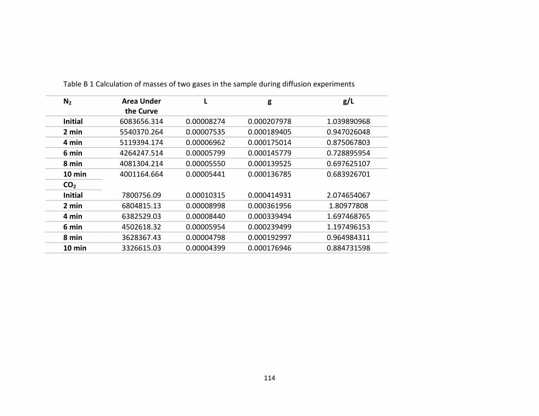
114
Table B 1 Calculation of masses of two gases in the sample during diffusion experiments
N2 Area Under the Curve
L g g/L
Initial 6083656.314 0.00008274 0.000207978 1.039890968
2 min 5540370.264 0.00007535 0.000189405 0.947026048
4 min 5119394.174 0.00006962 0.000175014 0.875067803
6 min 4264247.514 0.00005799 0.000145779 0.728895954
8 min 4081304.214 0.00005550 0.000139525 0.697625107
10 min 4001164.664 0.00005441 0.000136785 0.683926701
CO2
Initial 7800756.09 0.00010315 0.000414931 2.074654067
2 min 6804815.13 0.00008998 0.000361956 1.80977808
4 min 6382529.03 0.00008440 0.000339494 1.697468765
6 min 4502618.32 0.00005954 0.000239499 1.197496153
8 min 3628367.43 0.00004798 0.000192997 0.964984311
10 min 3326615.03 0.00004399 0.000176946 0.884731598

115
Table B 2 Calculation of masses of two gases in the sample during solubility experiments
N2 Area Under the Curve Initial
Area Under the Curve Final
Volume in Liters Initial
Volume in Liters Final
Mass in g Initial
Mass in g Final
30338453.29 24670022.39 0.000412633 0.000335537 0.001037162 0.000843379
23420261.44 22470110.78 0.000318539 0.000305616 0.000800654 0.000768172
28023893.17 25468419.5 0.000381153 0.000346396 0.000958035 0.000870673
30705019.36 25629510.59 0.000417619 0.000348587 0.001049693 0.00087618
25323649.99 28981175.65 0.000344427 0.000394173 0.000865724 0.000990762
CO2
15254318.6 8941923.39 0.000201718 0.000118245 0.000811394 0.000475631
15773312.38 8230471.614 0.000208581 0.000108837 0.000839 0.000437788
13955661.99 8585441.282 0.000184545 0.000113531 0.000742317 0.000456669
11838321.61 66258408.34 0.000156546 0.000876179 0.000629693 0.003524358
10305841.78 5136473.106 0.000136281 0.000067923 0.000548179 0.000273215

116
Appendix C
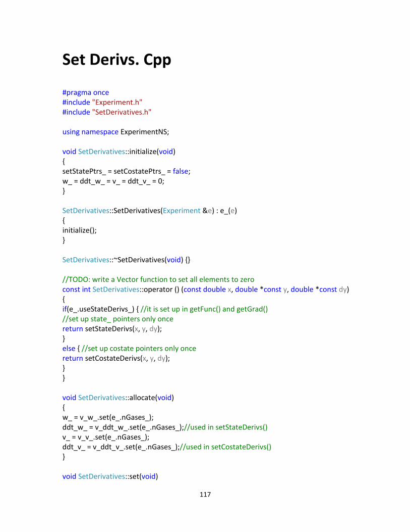
117
Set Derivs. Cpp
#pragma once #include "Experiment.h" #include "SetDerivatives.h" using namespace ExperimentNS; void SetDerivatives::initialize(void) { setStatePtrs_ = setCostatePtrs_ = false; w_ = ddt_w_ = v_ = ddt_v_ = 0; } SetDerivatives::SetDerivatives(Experiment &e) : e_(e) { initialize(); } SetDerivatives::~SetDerivatives(void) {} //TODO: write a Vector function to set all elements to zero const int SetDerivatives::operator () (const double x, double *const y, double *const dy) { if(e_.useStateDerivs_) { //it is set up in getFunc() and getGrad() //set up state_ pointers only once return setStateDerivs(x, y, dy); } else { //set up costate pointers only once return setCostateDerivs(x, y, dy); } } void SetDerivatives::allocate(void) { w_ = v_w_.set(e_.nGases_); ddt_w_ = v_ddt_w_.set(e_.nGases_);//used in setStateDerivs() v_ = v_v_.set(e_.nGases_); ddt_v_ = v_ddt_v_.set(e_.nGases_);//used in setCostateDerivs() } void SetDerivatives::set(void)
118
{ allocate(); } //------ functions called by operator() [i.e. SetDerivs() ] int SetDerivatives::setStateDerivs( const double x,//time double *const y,//gas mass fractions double *const dy) //d/dt(y) { // set pointers w_[0] = &y[0]; ddt_w_[0] = &dy[0];//for 1st gas w_[1] = &y[e_.nZminus1_]; ddt_w_[1] = &dy[e_.nZminus1_];//for 2nd gas unsigned i, j; for(i=0; i<e_.nGases_; i++) { for(j=0; j<e_.nZminus1_; j++) { if(w_[i][j] < -1e3) { return -1;//failed //puts("w_[i][j] < 0. in Experiment::setStateDerivs().."); } } } //state_ equations for ith gas; index of the other gas is k --------------- for(i=0; i<e_.nGases_; i++) { unsigned k;//index of the other gas k = (i==0) ? 1 : 0; for(j=0; j<e_.nZminus1_; j++) { double w3 = 1 - w_[i][j] - w_[k][j]; double w3_sqr = SQR(w3); double wibyw3 = w_[i][j]/w3; double wijMinus1 = w_[i][j-1]; double wkjMinus1 = w_[k][j-1]; if(j==0) { //at the grid point below the gas-liquid surface wijMinus1 = (*e_.intGasWvsTime_[i])(x); wkjMinus1 = (*e_.intGasWvsTime_[k])(x); } //for the ith gas double ddz_wi = (w_[i][j+1]-wijMinus1)/e_.dZ2_;
119
double ddz_wi_sqr=SQR(ddz_wi); //for the other gas of index k double ddz_wk = (w_[k][j+1]-wkjMinus1)/e_.dZ2_; double ddz_wk_sqr = SQR(ddz_wk); double d2dz2_wi, d2dz2_wk; if(j < e_.nZminus2_) { //for intermediate grid points d2dz2_wi = (w_[i][j+1]-2*w_[i][j]+wijMinus1)/e_.dZsqr_; d2dz2_wk = (w_[k][j+1]-2*w_[k][j]+wkjMinus1)/e_.dZsqr_; } else { //at the bottom d2dz2_wi = 2*(w_[i][j-1]-w_[i][j])/e_.dZsqr_; d2dz2_wk = 2*(w_[k][j-1]-w_[k][j])/e_.dZsqr_; } double Dii = ( *e_.DvsGasMf_[i][i] ) ( w_[i][j], w_[k][j] ); double Dik = ( *e_.DvsGasMf_[i][k] ) ( w_[i][j], w_[k][j] ); double Dki = ( *e_.DvsGasMf_[k][i] ) ( w_[i][j], w_[k][j] ); double Dkk = ( *e_.DvsGasMf_[k][k] ) ( w_[i][j], w_[k][j] ); double ddwi_Dii = ( *e_.dDvsGasMf_[i][i][i] ) ( w_[i][j],w_[k][j] ); double ddwk_Dii = ( *e_.dDvsGasMf_[i][i][k] ) ( w_[i][j],w_[k][j] ); double ddwi_Dik = ( *e_.dDvsGasMf_[i][k][i] ) ( w_[i][j],w_[k][j] ); double ddwk_Dik = ( *e_.dDvsGasMf_[i][k][k] ) ( w_[i][j],w_[k][j] ); double ddwi_Dki = ( *e_.dDvsGasMf_[k][i][i] ) ( w_[i][j],w_[k][j] ); double ddwk_Dki = ( *e_.dDvsGasMf_[k][i][k] ) ( w_[i][j],w_[k][j] ); double ddwi_Dkk = ( *e_.dDvsGasMf_[k][k][i] ) ( w_[i][j],w_[k][j] ); double ddwk_Dkk = ( *e_.dDvsGasMf_[k][k][k] ) ( w_[i][j],w_[k][j] ); if(j < e_.nZminus2_) { //for intermediate grid points //@@ state eqn double Dkkki = Dkk*ddz_wk + Dki*ddz_wi; double Diiik = Dii*ddz_wi + Dik*ddz_wk; ddt_w_[i][j] = ( Dkkki + Diiik ) * (1-w_[k][j])/w3_sqr*ddz_wi + ( Dkkki + Diiik ) * w_[i][j]/w3_sqr*ddz_wk + ( Dki*w_[i][j] + (1-w_[k][j])*Dii ) / w3*d2dz2_wi + ( Dkk*w_[i][j] + (1-w_[k][j])*Dki ) / w3*d2dz2_wk + ( w_[i][j]*(ddwi_Dkk + ddwk_Dki) + (1-w_[k][j])*(ddwk_Dii + ddwi_Dik) ) / w3*ddz_wi*ddz_wk + ( w_[i][j]*ddwi_Dki + (1-w_[k][j])*ddwi_Dii ) / w3*ddz_wi_sqr + ( (1-w_[k][j])*ddwk_Dik + w_[i][j]*ddwk_Dkk ) / w3*ddz_wk_sqr;
120
} else { //at the bottom ddt_w_[i][j] = ( Dki*w_[i][j] + (1-w_[k][j])*Dii ) / w3*d2dz2_wi + ( Dkk*w_[i][j] + (1-w_[k][j])*Dki ) / w3*d2dz2_wk; } } } for(i=0; i<e_.n_; i++) { if(!_finite(dy[i])) { return -1;//failed } } return 1; };//-- end of setStateDerivs() -- int SetDerivatives::setCostateDerivs( const double x,//time double *const y,//lambda double *const dy) { // set pointers v_[0] = &y[0]; ddt_v_[0] = &dy[0];//for 1st gas v_[1] = &y[e_.nZminus1_]; ddt_v_[1] = &dy[e_.nZminus1_];//for 2nd gas //costate equations for ith gas; index of the other gas is k --------------- unsigned i, j; for(i=0; i<e_.nGases_; i++) { double diff = (*e_.simGasMassAbsVsTime_[i])(x) - (*e_.expGasMassAbsVsTime_[i])(x); if (diff > 0.) diff *= e_.penalty_; double term1 = e_.wt_[i]*e_.factor_*( diff ); unsigned k;//index of the other gas k = (i==0) ? 1 : 0; for (j=0; j<e_.nZminus1_; j++) { //derivatives for costate variables --------------- double vijMinus1 = 0., vkjMinus1 = 0.; if(j==0) {//at the grid point below the gas-liquid surface vijMinus1 = 0;//BC vkjMinus1 = 0;//BC
121
} else { vijMinus1 = v_[i][j-1]; vkjMinus1 = v_[k][j-1]; } //for the ith gas double ddz_vi = (v_[i][j+1]-vijMinus1)/e_.dZ2_; double ddz_vi_sqr=SQR(ddz_vi); //for the other gas of index k double ddz_vk = (v_[k][j+1]-vkjMinus1)/e_.dZ2_; double ddz_vk_sqr = SQR(ddz_vk); double d2dz2_vi, d2dz2_vk; if(j < e_.nZminus2_) { //for intermediate grid points d2dz2_vi = (v_[i][j+1]-2*v_[i][j]+vijMinus1)/e_.dZsqr_; d2dz2_vk = (v_[k][j+1]-2*v_[k][j]+vkjMinus1)/e_.dZsqr_; } else { //at the bottom d2dz2_vi = 2*(v_[i][j-1]-v_[i][j])/e_.dZsqr_; d2dz2_vk = 2*(v_[k][j-1]-v_[k][j])/e_.dZsqr_; } //derivatives for state_ variables --------------- double wij = (*e_.stateVsTime_[i][j])(x); double wkj = (*e_.stateVsTime_[k][j])(x); double w3 = 1 - wij - wkj; double w3_sqr = SQR(w3); double w3_cub = CUB(w3); double wibyw3 = wij/w3; double wkbyw3 = wkj/w3; double wijMinus1 = 0., wkjMinus1 = 0.; if(j==0) { //at the grid point below the gas-liquid surface wijMinus1 = (*e_.intGasWvsTime_[i])(x); wkjMinus1 = (*e_.intGasWvsTime_[k])(x); } else { double wijMinus1 = (*e_.stateVsTime_[i][j-1])(x); double wkjMinus1 = (*e_.stateVsTime_[k][j-1])(x); } double ddz_wi, ddz_wi_sqr, ddz_wk, ddz_wk_sqr, d2dz2_wi, d2dz2_wk; if(j < e_.nZminus2_) { //for intermediate grid points double wijPlus1 = (*e_.stateVsTime_[i][j+1])(x);
122
//for the ith gas ddz_wi = (wijPlus1-wijMinus1)/e_.dZ2_; ddz_wi_sqr=SQR(ddz_wi); double wkjPlus1 = (*e_.stateVsTime_[k][j+1])(x); //for the other gas of index k ddz_wk = (wkjPlus1-wkjMinus1)/e_.dZ2_; ddz_wk_sqr = SQR(ddz_wk); d2dz2_wi = (wijPlus1-2*wij+wijMinus1)/e_.dZsqr_; d2dz2_wk = (wkjPlus1-2*wkj+wkjMinus1)/e_.dZsqr_; } else { //at the bottom ddz_wi = ddz_wi_sqr = ddz_wk = ddz_wk_sqr = 0.;
//1st derivs are zero d2dz2_wi = 2*(wijMinus1-wij)/e_.dZsqr_; d2dz2_wk = 2*(wkjMinus1-wkj)/e_.dZsqr_; } double Dii = (*e_.DvsGasMf_[i][i])(wij,wkj); double Dik = (*e_.DvsGasMf_[i][k])(wij,wkj); double Dki = (*e_.DvsGasMf_[k][i])(wij,wkj); double Dkk = (*e_.DvsGasMf_[k][k])(wij,wkj); double ddwi_Dii = (*e_.dDvsGasMf_[i][i][i])(wij,wkj);//d/dw[i] (Dii) double ddwk_Dii = (*e_.dDvsGasMf_[i][i][k])(wij,wkj);//d/dw[k] (Dii) double ddwi_Dik = (*e_.dDvsGasMf_[i][k][i])(wij,wkj);//d/dw[i] (Dik) double ddwk_Dik = (*e_.dDvsGasMf_[i][k][k])(wij,wkj);//d/dw[k] (Dik) double ddwi_Dki = (*e_.dDvsGasMf_[k][i][i])(wij,wkj);//d/dw[i] (Dki) double ddwk_Dki = (*e_.dDvsGasMf_[k][i][k])(wij,wkj);//d/dw[k] (Dki) double ddwi_Dkk = (*e_.dDvsGasMf_[k][k][i])(wij,wkj);//d/dw[i] (Dkk) double ddwk_Dkk = (*e_.dDvsGasMf_[k][k][k])(wij,wkj);//d/dw[k] (Dkk) //2nd dervatives of Dijs double d2dwi2_Dkk = ( (*e_.dDvsGasMf_[k][k][i])(1.001*wij,wkj)
- ddwi_Dkk ) * 1e-3; double d2dwidwk_Dki = ( (*e_.dDvsGasMf_[k][i][i])(1.001*wij,wkj)
- ddwk_Dki ) * 1e-3; double d2dwidwk_Dii = ( (*e_.dDvsGasMf_[i][i][k])(1.001*wij,wkj)
- ddwk_Dii ) * 1e-3; double d2dwi2_Dik = ( (*e_.dDvsGasMf_[i][k][i])(1.001*wij,wkj)
- ddwi_Dik ) * 1e-3; double d2dwi2_Dki = ( (*e_.dDvsGasMf_[k][i][i])(1.001*wij,wkj)
123
- ddwi_Dki ) * 1e-3; double d2dwi2_Dii = ( (*e_.dDvsGasMf_[i][i][i])(1.001*wij,wkj)
- ddwi_Dii ) * 1e-3; double d2dwidwk_Dik = ( (*e_.dDvsGasMf_[i][k][k])(1.001*wij,wkj)
- ddwk_Dik ) * 1e-3; double d2dwidwk_Dkk = ( (*e_.dDvsGasMf_[k][k][k])(wij,wkj)
- ddwk_Dkk ) * 1e-3; //p.6 double Dkkki = Dkk*ddz_wk + Dki*ddz_wi; double Diiik = Dii*ddz_wi + Dik*ddz_wk; double ddz_Dkk = ddwi_Dkk*ddz_wi + ddwk_Dkk*ddz_wk; double ddz_Dki = ddwi_Dki*ddz_wi + ddwk_Dki*ddz_wk; double ddz_Dkkki = ddz_Dkk*ddz_wk + Dkk*d2dz2_wk + ddz_Dki*ddz_wi
+ Dki*d2dz2_wi; double ddz_Dii = ddwi_Dii*ddz_wi + ddwk_Dii*ddz_wk; double ddz_Dik = ddwi_Dik*ddz_wi + ddwk_Dik*ddz_wk; double ddz_Diiik = ddz_Dii*ddz_wi + Dii*d2dz2_wi + ddz_Dik*ddz_wk
+ Dik*d2dz2_wk; double DwiDkkki = ddwi_Dkk*ddz_wk + ddwi_Dki*ddz_wi; double DwiDiiik = ddwi_Dii*ddz_wi + ddwi_Dik*ddz_wk; double ddwi_fi = ( 2*(1-w_[k][j])/w3*(Dkkki+Diiik) + (1- w_[k][j])* (DwiDkkki + DwiDiiik) ) / w3_sqr*ddz_wi + ( (1+w_[i][j]-w_[k][j])/w3*Dkkki + (1+w_[i][j]-w_[k][j])/w3*Diiik + w_[i][j]*DwiDkkki + w_[i][j]*DwiDiiik ) / w3_sqr*ddz_wk + ( (1-w_[k][j])*Dki/w3 + (1-w_[k][j])*Dii/w3 + w_[i][j]*ddwi_Dki + (1-w_[k][j])*ddwi_Dii ) / w3*d2dz2_wi + ( (1-w_[k][j])*Dkk/w3 + (1-w_[k][j])*Dki/w3 + w_[i][j]*ddwi_Dkk + (1-w_[k][j])*ddwi_Dki ) / w3*d2dz2_wk + ( (1-w_[k][j])*ddwi_Dkk/w3 + (1- w_[k][j])*ddwk_Dki/w3 + (1-w_[k][j])/w3*ddwk_Dii + (1-w_[k][j])*ddwi_Dik/w3 + w_[i][j]*d2dwi2_Dkk + w_[i][j]*d2dwidwk_Dki + (1-w_[k][j])*d2dwidwk_Dii + (1-w_[k][j])*d2dwi2_Dik ) / w3*ddz_wi*ddz_wk + ( (1-w_[k][j])*ddwi_Dki/w3 + (1-w_[k][j])*ddwi_Dii/w3 + w_[i][j]*d2dwi2_Dki + (1-w_[k][j])*d2dwi2_Dii ) /w3 * ddz_wi_sqr + ( (1-w_[k][j])*ddwk_Dik/w3 + (1-w_[k][j])*ddwk_Dkk/w3 + (1-w_[k][j])*d2dwidwk_Dik + w_[i][j]*d2dwidwk_Dkk ) /w3 * ddz_wk_sqr; //p.6 double ddwi_fk = ( -1/w3_sqr + (1-w_[i][j])/w3_cub )*Diiik*ddz_wk + (1-w_[i][j])/w3_sqr*DwiDiiik*ddz_wk
124
+ ( -1/w3_sqr + (1-w_[i][j])/w3_cub )*Dkkki*ddz_wk + (1-w_[i][j])/w3_sqr*DwiDkkki*ddz_wk + w_[k][j]/w3_cub*Diiik*ddz_wi + w_[k][j]/w3_sqr*DwiDiiik*ddz_wi + w_[k][j]/w3_cub*Dkkki*ddz_wi + w_[k][j]/w3_sqr*DwiDkkki*ddz_wi + ddwi_Dik*w_[k][j]/w3*d2dz2_wk + Dik*w_[k][j]/w3_sqr*d2dz2_wk + ddwi_Dkk*(1-w_[i][j])/w3*d2dz2_wk + Dkk*(-1/w3 + (1-w_[i][j])/w3_sqr)*d2dz2_wk + ddwi_Dii*w_[k][j]/w3*d2dz2_wi + Dii*w_[k][j]/w3_sqr*d2dz2_wi + ddwi_Dik*(1-w_[i][j])/w3*d2dz2_wi + Dik*(-1/w3 + (1-w_[i][j])/w3_sqr)*d2dz2_wi + (w_[k][j]/w3_sqr*ddwk_Dii + w_[k][j]/w3*d2dwidwk_Dii)*ddz_wi*ddz_wk + (w_[k][j]/w3_sqr*ddwi_Dik + w_[k][j]/w3*d2dwi2_Dik)*ddz_wi*ddz_wk + ( (-1/w3 + (1-w_[i][j])/w3_sqr)*ddwi_Dkk + (1-w_[i][j])/w3*d2dwi2_Dkk)*ddz_wi*ddz_wk + ( (-1/w3 + (1-w_[i][j])/w3_sqr)*ddwk_Dki + (1-w_[i][j])/w3*d2dwidwk_Dki)*ddz_wi*ddz_wk + (w_[k][j]/w3_sqr*ddwk_Dik + w_[k][j]/w3*d2dwidwk_Dik)*ddz_wk_sqr + ( (-1/w3 + (1-w_[i][j])/w3_sqr)*ddwk_Dkk + (1-w_[i][j])/w3*d2dwidwk_Dkk)*ddz_wk_sqr + ( (-1/w3 + (1-w_[i][j])/w3_sqr)*ddwi_Dki + (1-w_[i][j])/w3*d2dwi2_Dki)*ddz_wi_sqr + (w_[k][j]/w3_sqr*ddwi_Dii + w_[k][j]/w3*d2dwidwk_Dii)*ddz_wi_sqr; double ddwiz_fi = (1-w_[k][j])*(Dkkki + Diiik + Dki + Dii) / w3_sqr*ddz_wi + w_[i][j]*(Dki+Dii) / w3_sqr*ddz_wk +(w_[i][j]*(ddwi_Dkk + ddwk_Dki) + (1-w_[k][j])*(ddwk_Dii + ddwi_Dik) )/ w3*ddz_wk +2*(w_[i][j]*ddwi_Dki + (1-w_[k][j])*ddwi_Dii)/ w3*ddz_wi; //p.7 double d2dzdwi_Dkk = d2dwi2_Dkk*ddz_wi + d2dwidwk_Dkk*ddz_wk; double d2dwk2_Dki = ( (*e_.dDvsGasMf_[k][i][k])(wij,1.003*wkj) - ddwk_Dki ) * 1e-3; double d2dwk2_Dik = ( (*e_.dDvsGasMf_[i][k][k])(wij,1.003*wkj) - ddwk_Dik ) * 1e-3; double d2dzdwk_Dki = d2dwk2_Dki*ddz_wk + d2dwidwk_Dki*ddz_wi; double d2dzdwk_Dik = d2dwk2_Dik*ddz_wk + d2dwidwk_Dik*ddz_wi;
125
double d2dwk2_Dii = ( (*e_.dDvsGasMf_[i][i][k])(wij,1.003*wkj) - ddwk_Dii ) * 1e-3; double d2dzdwk_Dii = d2dwk2_Dii*ddz_wk + d2dwidwk_Dii*ddz_wi; double d2dzdwi_Dik = d2dwi2_Dik*ddz_wi + d2dwidwk_Dik*ddz_wk; double d2dzdwi_Dki = d2dwi2_Dki*ddz_wi + d2dwidwk_Dki*ddz_wk; double d2dzdwi_Dii = d2dwi2_Dki*ddz_wi + d2dwidwk_Dii*ddz_wk; double d2dzdwiz_fi = -ddz_wk*(Dkkki + Diiik + Dki + Dii) / w3_sqr*ddz_wi + (1-w_[k][j])*(ddz_Dkkki + ddz_Diiik + ddz_Dki + ddz_Dii) / w3_sqr*ddz_wi + (1-w_[k][j])*(Dkkki + Diiik + Dki + Dii)* 2*w3*(ddz_wi+ddz_wk)/w3_cub *ddz_wi + (1-w_[k][j])*(Dkkki + Diiik + Dki + Dii) / w3_sqr*d2dz2_wi + ddz_wi*(Dki+Dii) / w3_sqr*ddz_wk + w_[i][j]*(ddz_Dki + ddz_Dii) / w3_sqr*ddz_wk + w_[i][j]*(Dki+Dii)* 2*w3*(ddz_wi+ddz_wk)/w3_cub *ddz_wk + w_[i][j]*(Dki+Dii) / w3_sqr*d2dz2_wk +( ddz_wi*(ddwi_Dkk + ddwk_Dki) + w_[i][j]*(d2dzdwi_Dkk + d2dzdwk_Dki) -ddz_wk*(ddwk_Dii + ddwi_Dik) + (1-w_[k][j])*(d2dzdwk_Dii + d2dzdwi_Dik) )/ w3*ddz_wk +(w_[i][j]*(ddwi_Dkk + ddwk_Dki) + (1-w_[k][j])*(ddwk_Dii + ddwi_Dik) )* 2*w3*(ddz_wi+ddz_wk)/w3_cub *ddz_wk +(w_[i][j]*(ddwi_Dkk + ddwk_Dki) + (1-w_[k][j])*(ddwk_Dii + ddwi_Dik) )/ w3*d2dz2_wk +2*( ddz_wi*ddwi_Dki + w_[i][j]*d2dzdwi_Dki - ddz_wk*ddwi_Dii + (1-w_[k][j])*d2dzdwi_Dii )/ w3*ddz_wi +2*(w_[i][j]*ddwi_Dki + (1-w_[k][j])*ddwi_Dii)* 2*w3*(ddz_wi+ddz_wk)/w3_cub *ddz_wi +2*(w_[i][j]*ddwi_Dki + (1-w_[k][j])*ddwi_Dii)/ w3*d2dz2_wi; double ddwizz_fi = (Dki*w_[i][j] + (1-w_[k][j])*Dii) /w3; // p.11 double d2dzdwizz_fi = ( w_[i][j]*ddz_Dki + (1-w_[k][j])*ddz_Dii + ((1-w_[k][j])/w3*ddz_wi + w_[i][j]/w3*ddz_wk)*Dki + (2*(1-w_[k][j])/w3*ddz_wi + ddz_wk )*Dii )/w3; //p.15 double d2dz2_Dki = ddwi_Dki*d2dz2_wi + d2dzdwi_Dki*ddz_wi + ddwk_Dki*d2dz2_wk + d2dzdwk_Dki*ddz_wk; double d2dz2_Dii = ddwi_Dii*d2dz2_wi + d2dzdwi_Dii*ddz_wi + ddwk_Dii*d2dz2_wk + d2dzdwk_Dii*ddz_wk;
126
double d2dz2_Dik = ddwi_Dik*d2dz2_wi + d2dzdwi_Dik*ddz_wi + ddwk_Dik*d2dz2_wk + d2dzdwk_Dik*ddz_wk; double d3dz2dwizz_fi = ( ddz_wi*ddz_Dki + w_[i][j]*d2dz2_Dki - ddz_wk*ddz_Dii + (1-w_[k][j])*d2dz2_Dii + ((1-w_[k][j])/w3*ddz_wi + w_[i][j]/w3*ddz_wk)*ddz_Dki + + ( (1-w_[k][j])/w3_sqr*ddz_wi + (-1/w3 + (1-w_[k][j])/w3_sqr)*ddz_wk + (1-w_[k][j])/w3*d2dz2_wi + (1/w3 + w_[i][j]/w3_sqr)*ddz_wi + w_[i][j]/w3_sqr*ddz_wk + w_[i][j]/w3*d2dz2_wk )*Dki + ((1-w_[k][j])/w3*ddz_wi + w_[i][j]/w3*ddz_wk)*ddz_Dki + ( 2*( (1-w_[k][j])/w3_sqr*ddz_wi + (-1/w3 + (1-w_[k][j])/w3_sqr)*ddz_wk )*ddz_wi + 2*(1-w_[k][j])/w3*d2dz2_wi + d2dz2_wk )*Dii + (2*(1-w_[k][j])/w3*ddz_wi + ddz_wk )*ddz_Dii )/w3 + + d2dzdwizz_fi/w3*(ddz_wi+ddz_wk); double ddwiz_fk = (1-w_[i][j])/w3_sqr*Dii*ddz_wk + (1-w_[i][j])/w3_sqr*Dki*ddz_wk + 2*w_[k][j]/w3_sqr*Dii*ddz_wi + 2*w_[k][j]/w3_sqr*Dki*ddz_wi + w_[k][j]/w3*ddwk_Dii*ddz_wk + w_[k][j]/w3*ddwi_Dik*ddz_wk + (1-w_[i][j])/w3*ddwi_Dkk*ddz_wk + (1-w_[i][j])/w3*ddwk_Dki*ddz_wk + 2*(1-w_[i][j])/w3*ddwi_Dki*ddz_wi + 2*w_[k][j]/w3*ddwi_Dii*ddz_wi; //double ddwiz_fk = (1-w_[i][j])/w3_sqr*(Dii*ddz_wk + Dki*ddz_wk) // + 2*w_[k][j]/w3_sqr*(Dii*ddz_wi + Dki*ddz_wi) // + w_[k][j]/w3*(ddwk_Dii*ddz_wk + ddwi_Dik*ddz_wk + 2*ddwi_Dii*ddz_wi) // + (1-w_[i][j])/w3*(ddwi_Dkk*ddz_wk + ddwk_Dki*ddz_wk + 2*ddwi_Dki*ddz_wi); double d2dzdwiz_fk = ((1-w_[i][j]+w_[k][j])/w3_cub*ddz_wi + 2*(1-w_[i][j])/w3_cub*ddz_wk)*(Dii*ddz_wk + Dki*ddz_wk) + (1-w_[i][j])/w3_sqr*(ddz_Dii*ddz_wk + Dii*d2dz2_wk + ddz_Dki*ddz_wk + Dki*d2dz2_wk) + 2*(2*w_[k][j]/w3_cub*ddz_wi + (1-w_[i][j]+w_[k][j])/w3_cub*ddz_wk)*(Dii*ddz_wi + Dki*ddz_wi) + 2*w_[k][j]/w3_sqr*(ddz_Dii*ddz_wi + Dii*d2dz2_wi + ddz_Dki*ddz_wi + Dki*d2dz2_wi) + (w_[k][j]/w3_sqr*ddz_wi + (1-w_[i][j])/w3_sqr*ddz_wk)*(ddwk_Dii*ddz_wk + ddwi_Dik*ddz_wk + 2*ddwi_Dii*ddz_wi) + w_[k][j]/w3*(d2dzdwk_Dii*ddz_wk + ddwk_Dii*d2dz2_wk + d2dzdwi_Dik*ddz_wk + ddwi_Dik*d2dz2_wk

127
+ 2*d2dzdwi_Dii*ddz_wi + 2*ddwi_Dii*d2dz2_wi) + (w_[k][j]/w3_sqr*ddz_wi + (1-w_[i][j])/w3_sqr*ddz_wk)*(ddwi_Dkk*ddz_wk + ddwk_Dki*ddz_wk + 2*ddwi_Dki*ddz_wi) + (1-w_[i][j])/w3*(d2dzdwi_Dkk*ddz_wk + ddwi_Dkk*d2dz2_wk + d2dzdwk_Dki*ddz_wk + ddwk_Dki*d2dz2_wk + 2*d2dzdwi_Dki*ddz_wi + 2*ddwi_Dki*d2dz2_wi); double ddwizz_fk = ( Dii*w_[k][j] + Dik*(1-w_[i][j]) )/w3; double d2dzdwizz_fk = ( ddz_Dii*w_[k][j] + Dii*ddz_wk + ddz_Dik*(1-w_[i][j]) - Dik*ddz_wi) /w3 + ddwizz_fk/w3*(ddz_wi + ddz_wk); double d3dz2dwizz_fk = ( d2dz2_Dii*w_[k][j] + ddz_Dii*ddz_wk + ddz_Dii*ddz_wk + Dii*d2dz2_wk + d2dz2_Dik*(1-w_[i][j]) - ddz_Dik*ddz_wi - ddz_Dik*ddz_wi - Dik*d2dz2_wi ) /w3 + ( ddz_Dii*w_[k][j] + Dii*ddz_wk + ddz_Dik*(1-w_[i][j]) - Dik*ddz_wi) /w3_sqr*(ddz_wi + ddz_wk) + ( ddz_Dii*w_[k][j] + Dii*ddz_wk + ddz_Dik*(1-w_[i][j]) - Dik*ddz_wi)/w3_sqr*(ddz_wi + ddz_wk) + ( Dii*w_[k][j] + Dik*(1-w_[i][j]) )* 2/w3_cub*(ddz_wi + ddz_wk) *(ddz_wi + ddz_wk) + ( Dii*w_[k][j] + Dik*(1-w_[i][j]) )/w3_sqr*(d2dz2_wi + d2dz2_wk); //@@ check term1 if(j < e_.nZminus2_) { //for intermediate grid points ddt_v_[i][j] = term1 - v_[i][j]*ddwi_fi + ddz_vi*ddwiz_fi + v_[i][j]*d2dzdwiz_fi - d2dz2_vi*ddwizz_fi - 2*ddz_vi*d2dzdwizz_fi - v_[i][j]*d3dz2dwizz_fi +v_[k][j]*ddwi_fk - ddz_vk*ddwiz_fk - v_[k][j]*d2dzdwiz_fk + d2dz2_vk*ddwizz_fk + 2*ddz_vk*d2dzdwizz_fk + v_[k][j]*d3dz2dwizz_fk; } else { //at the bottom ddt_v_[i][j] = term1 - v_[i][j]*ddwi_fi + v_[i][j]*d2dzdwiz_fi - d2dz2_vi*ddwizz_fi - v_[i][j]*d3dz2dwizz_fi +v_[k][j]*ddwi_fk - ddz_vk*ddwiz_fk - v_[k][j]*d2dzdwiz_fk + d2dz2_vk*ddwizz_fk + v_[k][j]*d3dz2dwizz_fk;
128
} } } //for(i=0; i<e_.n_; i++) dy[i] *= 1e-5; for(i=0; i<e_.n_; i++) { if(!_finite(dy[i])) { return -1;//failed } } return 1; };//-- end of setCostateDerivs() –
Set Derives. h
#pragma once #include "..\Vector\Vector.h" using namespace VectorNS; namespace ExperimentNS { class Experiment; class SetDerivatives { Experiment &e_; bool setStatePtrs_, setCostatePtrs_; Vec<double*> v_w_, v_ddt_w_,//used in setStateDerivs() v_v_, v_ddt_v_;//used in setCostateDerivs() double **w_, **ddt_w_, **v_, **ddt_v_; void initialize(void); void allocate(void); int setStateDerivs( const double x,//time double *const y,//gas mass fractions double *const dy) //d/dt(y) ;
129
int setCostateDerivs( const double x,//time double *const y,//lambda double *const dy) ;//-- end of setCostateDerivs() -- public: SetDerivatives(Experiment &e); ~SetDerivatives(void); void set(void); //------ function called by de object [as SetDerivs() ] const int operator () (const double x, double *const y, double *const dy); };//--- end of class SetDerivatives --- }// --- end of ExperimentNS ---
Get Gradient.Cpp
#pragma once #include "Experiment.h" #include "GetGradient.h" using namespace ExperimentNS; void GetGradient::initialize() { W_ = V_ = 0; tmpW_ = vD_ = 0; dD_ = 0; } __forceinline void GetGradient::allocate(void) { vD_ = v2d_vD_.set(e_.nGases_, e_.nZminus1_); dD_ = v4d_dD_.set(e_.nGases_, e_.nGases_, e_.nDvsGasMf_, e_.nDvsGasMf_); W_ = v_W_.set(e_.nGases_);
130
V_ = v_V_.set(e_.nGases_); W_[0] = &e_.state_[0]; //for 1st gas W_[1] = &e_.state_[e_.nZminus1_]; //for 2nd gas V_[0] = &e_.coState_[0]; //for 1st gas V_[1] = &e_.coState_[e_.nZminus1_]; //for 2nd gas //used in Accumulate_dD() tmpW_ = v2d_tmpW_.set(e_.nGases_, e_.nZminus1_); } GetGradient::GetGradient(Experiment &e) : e_(e) { initialize(); } void GetGradient::set() { allocate(); } GetGradient::~GetGradient(void){ } const bool GetGradient::operator() (double ****const D,//IN: optimization parameter ie diffusivity double *const grad)//OUT: gradient { e_.useStateDerivs_ = false;//for use in SetDerivs() //todo: set pointers to dD[] and d2D[] in Model unsigned i, j, k, l, m, n; for(i=0; i<e_.nZminus1_; i++) for(j=0; j<e_.nSamples_; j++) e_.coState_[i][j] = 0.; if(e_.de_->Solve(e_.coState_) != 1)//OUT: costate[n][nSamples_] variables error("Experiment::getGrad() failed.."); for(i=0; i<e_.nGases_; i++) for(j=0; j<e_.nGases_; j++) for(k=0; k<e_.nDvsGasMf_; k++) for(l=0; l<e_.nDvsGasMf_; l++) dD_[i][j][k][l] = 0.; for(i=0; i<e_.nGases_; i++) { k = (i==0) ? 1 : 0;//index of the other gas n = (i==0) ? 1 : 0;//index of the other gas; for use in vD_ //for(l=0; l<e_.nSamples_; l++) { for(l=1; l<e_.nSamples_-1; l++) {// exclude initial and final times when variational derivatives are not needed (at final time) or useful (at initial time)
131
for(j=0; j<e_.nZminus1_; j++) { double W3 = 1 - W_[i][j][l] - W_[k][j][l]; double WibyW3 = W_[i][j][l]/W3; double WkbyW3 = W_[k][j][l]/W3; double WijMinus1 = 0., WkjMinus1 = 0.; if(j == 0) { //at the grid point below the gas-liquid surface WijMinus1 = e_.intGasW_[i][l]; WkjMinus1 = e_.intGasW_[k][l]; } else { WijMinus1 = W_[i][j-1][l]; WkjMinus1 = W_[k][j-1][l]; } double ddz_Wi, ddz_Wi_sqr, ddz_Wk, ddz_Wk_sqr, d2dz2_Wi, d2dz2_Wk; if(j < e_.nZminus2_) { //for intermediate grid points ddz_Wi = (W_[i][j+1][l] - WijMinus1)/e_.dZ2_;
//for the ith gas ddz_Wi_sqr = SQR(ddz_Wi); ddz_Wk = (W_[k][j+1][l] - WkjMinus1)/e_.dZ2_;
//for the other gas of index k ddz_Wk_sqr = SQR(ddz_Wk); d2dz2_Wi = (W_[i][j+1][l]-2*W_[i][j][l]+WijMinus1)/e_.dZsqr_; d2dz2_Wk = (W_[k][j+1][l]-2*W_[k][j][l]+WkjMinus1)/e_.dZsqr_; } else { //at the bottom ddz_Wi = ddz_Wi_sqr = ddz_Wk = ddz_Wk_sqr = 0.;
//1st derivs are zero d2dz2_Wi = 2*(W_[i][j-1][l]-W_[i][j][l])/e_.dZsqr_; d2dz2_Wk = 2*(W_[k][j-1][l]-W_[k][j][l])/e_.dZsqr_; } double t1 = (1+1/W3); vD_[i][j] = -V_[i][j][l]*( (1-W_[k][j][l])/W3*ddz_Wi_sqr + W_[i][j][l]/W3*ddz_Wi*ddz_Wk + (1-W_[k][j][l])*d2dz2_Wi //ddD00_f1 /*ddD00_f2*/+ (1-W_[i][j][l])/W3*ddz_Wi*ddz_Wk + W_[i][j][l]/W3*ddz_Wi_sqr + W_[k][j][l]/W3*d2dz2_Wi ) /W3; //coeff of delta D01 (and delta D10 in the next outermost iteration) vD_[n][j] = -V_[i][j][l]*( ( (1-W_[k][j][l])*ddz_Wi*ddz_Wk + W_[i][j][l]*ddz_Wk_sqr )/W3 //ddD01_f1

132
/*ddD01_f2*/+ (1-W_[i][j][l])/W3*ddz_Wk_sqr + W_[k][j][l]/W3*ddz_Wi*ddz_Wk + W_[k][j][l]*d2dz2_Wk )/W3; if(!_finite(vD_[0][j]) || !_finite(vD_[1][j])) { puts ("infinite value .."); } }//-- loop over depth j -- //accumulate values of dD_[nGases_][nGases_][nDvsGasMf_][nDvsGasMf_] Accumulate_dD( i,//ith gas, 0 or 1 l,//time index vD_);//coeff of delta Dij }//-- loop over time l -- }//-- loop over gas i -- for(i=m=0; i<e_.nGases_; i++) for(j=0; j<e_.nGases_; j++) for(k=0; k<e_.nDvsGasMf_; k++) for(l=0; l<e_.nDvsGasMf_; l++) { grad[m++] = dD_[i][j][k][l]/e_.nSamples_; if(!_finite(dD_[i][j][k][l])) { puts ("infinite value .."); } } return true; }//-- end of operator() -- void GetGradient::Accumulate_dD( const unsigned i, //row index of the D matrix const unsigned iT, //time instant double **const vD) //coeff of delta Dij, vD[nGases_][nZminus1_] { unsigned j, k, l; for(j=0; j<e_.nGases_; j++) {// jth column of ith gas for(k=0; k<e_.nZminus1_; k++) { tmpW_[0][k] = W_[0][k][iT]; tmpW_[1][k] = W_[1][k][iT]; } dDvsW0W1_.set(tmpW_[0], tmpW_[1], vD[j], 5);
133
//interpolate or extrapolate at each grid point on the base of the 3d graph dD_ vs W0 and W1 for(k=0; k<e_.nDvsGasMf_; k++) { for(l=0; l<e_.nDvsGasMf_; l++) { double val = dDvsW0W1_( e_.p_gasMf_[0][k], e_.p_gasMf_[1][l] ); if(!_finite(val)) { puts ("infinite value .."); } dD_[i][j][k][l] += ( val ); } } } }
Get Gradient .h
#pragma once #include "..\Vector\Vector.h" #include "..\Spline\Krig.h" using namespace VectorNS; using namespace KrigNS; namespace ExperimentNS { class Experiment; /*~~~~~~~~~~~~~~~~~~~~~~~~~~~~~~~~~~~~~~~~~~~~~~~~~~~~~~~~~~~~~~~~~~~~~~~~ Aim: provide getGrad() while maintaining the state of some variables during iterations Usage: GetGradient getGrad; getGrad();//uses overloaded operator() Comments: 1. friend class of Experiment ~~~~~~~~~~~~~~~~~~~~~~~~~~~~~~~~~~~~~~~~~~~~~~~~~~~~~~~~~~~~~~~~~~~~~~~~~*/
134
class GetGradient { Experiment &e_; Vec<double**> v_W_, v_V_;//used in getGrad() double ***W_, ***V_; Vec2d<double> v2d_tmpW_,//used in Accumulate_dD() v2d_vD_;//used in getGrad() double **tmpW_, **vD_; Vec4d<double> v4d_dD_;//[nGases_][nGases_][nDvsGasMf_][nDvsGasMf_] double ****dD_;//used in getGrad() Krig dDvsW0W1_; void initialize(void); void allocate(void); public: GetGradient(Experiment &e); void set(void); ~GetGradient(void); //returns whether the call was successful; gradients are returned in grad[] const bool operator() (double ****const D,//IN: optimization parameter ie diffusivity double *const grad)//OUT: gradient ; //called by getGrad() to set dD_[i][0][nDvsGasMf_][nDvsGasMf_] void Accumulate_dD( const unsigned i,//row index of the D matrix const unsigned nT_,//time instant double **const vD)//vD[nGases_][nSamples_], e.g. vD_00 and vD_01 ; };//--- end of class GetGradient --- }// --- end of ExperimentNS ---
135
Appendix D
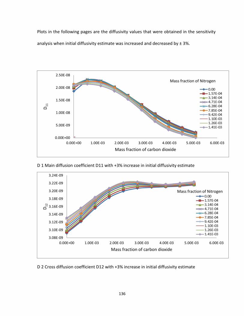
136
Plots in the following pages are the diffusivity values that were obtained in the sensitivity
analysis when initial diffusivity estimate was increased and decreased by ± 3%.
D 1 Main diffusion coefficient D11 with +3% increase in initial diffusivity estimate
D 2 Cross diffusion coefficient D12 with +3% increase in initial diffusivity estimate
0.00E+00
5.00E-09
1.00E-08
1.50E-08
2.00E-08
2.50E-08
0.00E+00 1.00E-03 2.00E-03 3.00E-03 4.00E-03 5.00E-03 6.00E-03
D1
1
Mass fraction of carbon dioxide
Mass fraction of Nitrogen
3.08E-09
3.10E-09
3.12E-09
3.14E-09
3.16E-09
3.18E-09
3.20E-09
3.22E-09
3.24E-09
0.00E+00 1.00E-03 2.00E-03 3.00E-03 4.00E-03 5.00E-03 6.00E-03
D1
2
Mass fraction of carbon dioxide
Mass fraction of Nitrogen
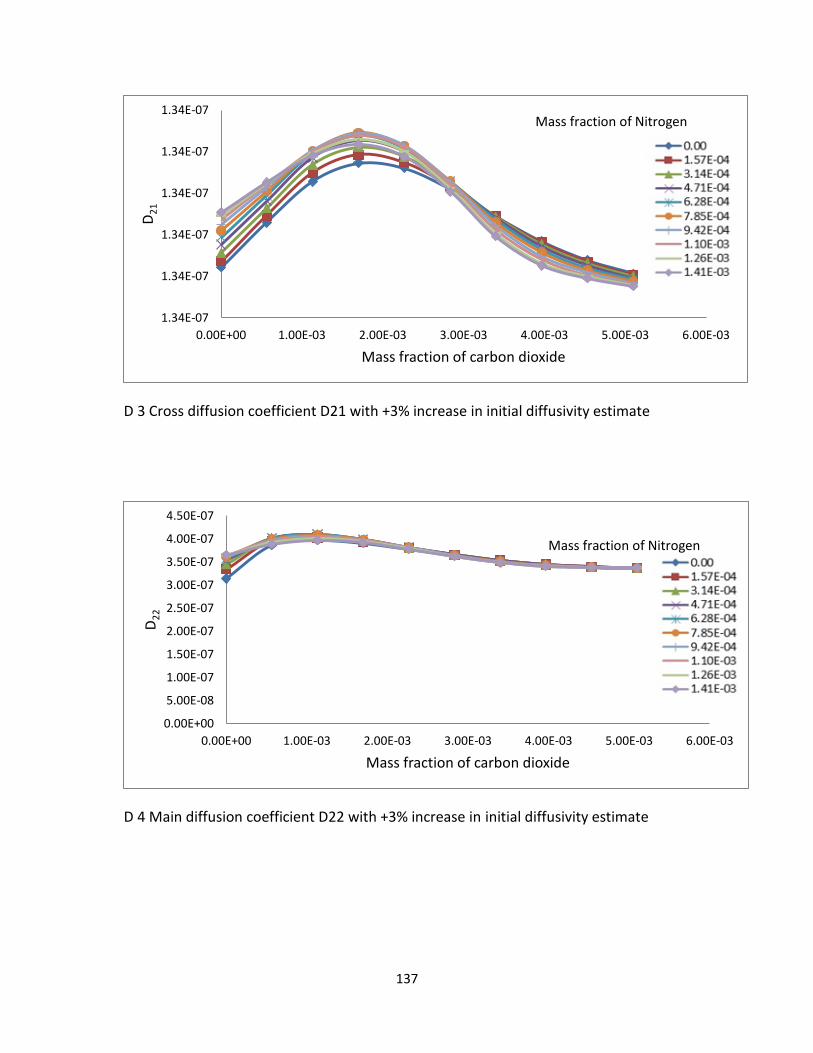
137
D 3 Cross diffusion coefficient D21 with +3% increase in initial diffusivity estimate
D 4 Main diffusion coefficient D22 with +3% increase in initial diffusivity estimate
1.34E-07
1.34E-07
1.34E-07
1.34E-07
1.34E-07
1.34E-07
0.00E+00 1.00E-03 2.00E-03 3.00E-03 4.00E-03 5.00E-03 6.00E-03
D2
1
Mass fraction of carbon dioxide
0.00E+00
5.00E-08
1.00E-07
1.50E-07
2.00E-07
2.50E-07
3.00E-07
3.50E-07
4.00E-07
4.50E-07
0.00E+00 1.00E-03 2.00E-03 3.00E-03 4.00E-03 5.00E-03 6.00E-03
D2
2
Mass fraction of carbon dioxide
Mass fraction of Nitrogen
Mass fraction of Nitrogen
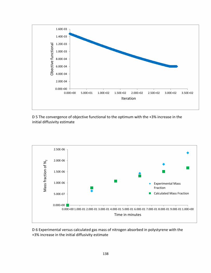
138
D 5 The convergence of objective functional to the optimum with the +3% increase in the initial diffusivity estimate
D 6 Experimental versus calculated gas mass of nitrogen absorbed in polystyrene with the +3% increase in the initial diffusivity estimate
0.00E+00
2.00E-04
4.00E-04
6.00E-04
8.00E-04
1.00E-03
1.20E-03
1.40E-03
1.60E-03
0.00E+00 5.00E+01 1.00E+02 1.50E+02 2.00E+02 2.50E+02 3.00E+02 3.50E+02
Ob
ecti
ve f
un
ctio
nal
Iteration
0.00E+00
5.00E-07
1.00E-06
1.50E-06
2.00E-06
2.50E-06
0.00E+00 1.00E-01 2.00E-01 3.00E-01 4.00E-01 5.00E-01 6.00E-01 7.00E-01 8.00E-01 9.00E-01 1.00E+00
Mas
s fr
acti
on
of
N2
Time in minutes
Experimental MassFraction
Calculated Mass Fraction
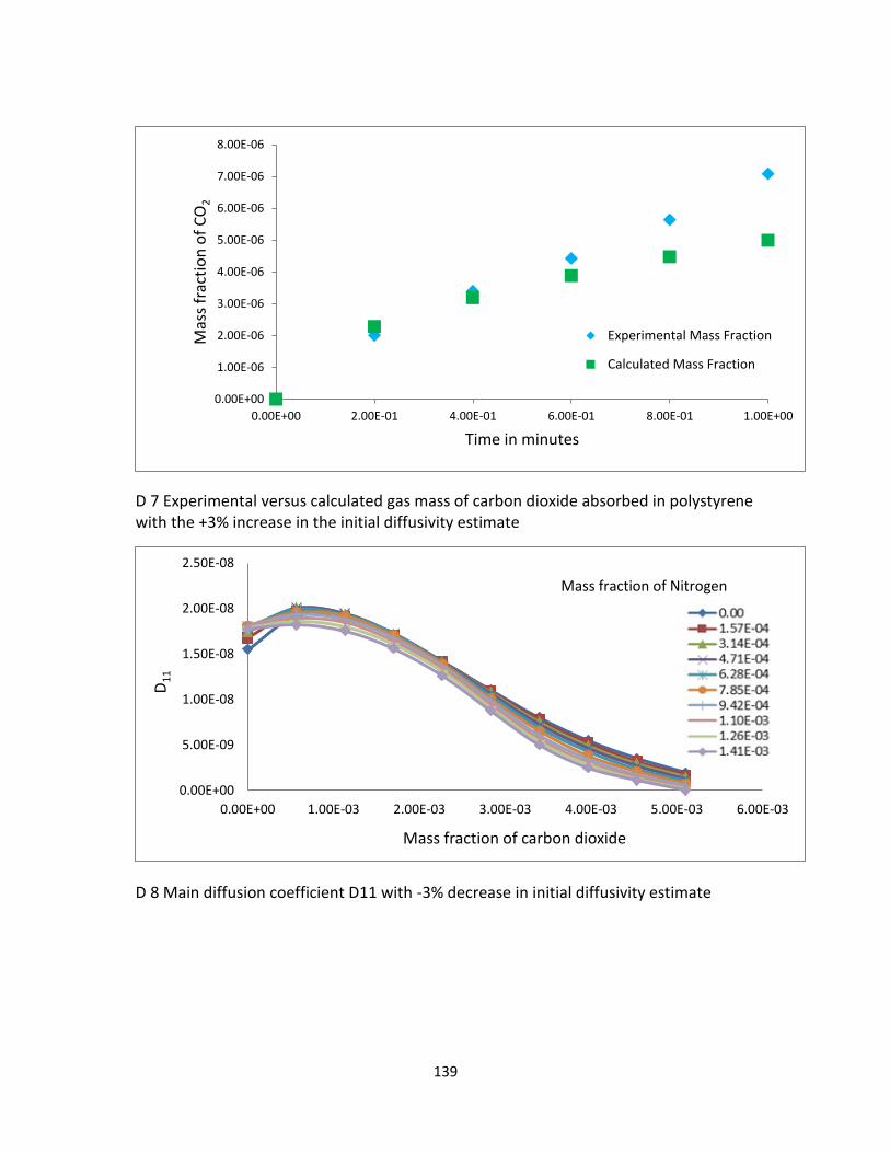
139
D 7 Experimental versus calculated gas mass of carbon dioxide absorbed in polystyrene with the +3% increase in the initial diffusivity estimate
D 8 Main diffusion coefficient D11 with -3% decrease in initial diffusivity estimate
0.00E+00
1.00E-06
2.00E-06
3.00E-06
4.00E-06
5.00E-06
6.00E-06
7.00E-06
8.00E-06
0.00E+00 2.00E-01 4.00E-01 6.00E-01 8.00E-01 1.00E+00
Mas
s fr
acti
on
of
CO
2
Time in minutes
Experimental Mass Fraction
Calculated Mass Fraction
0.00E+00
5.00E-09
1.00E-08
1.50E-08
2.00E-08
2.50E-08
0.00E+00 1.00E-03 2.00E-03 3.00E-03 4.00E-03 5.00E-03 6.00E-03
D1
1
Mass fraction of carbon dioxide
Mass fraction of Nitrogen
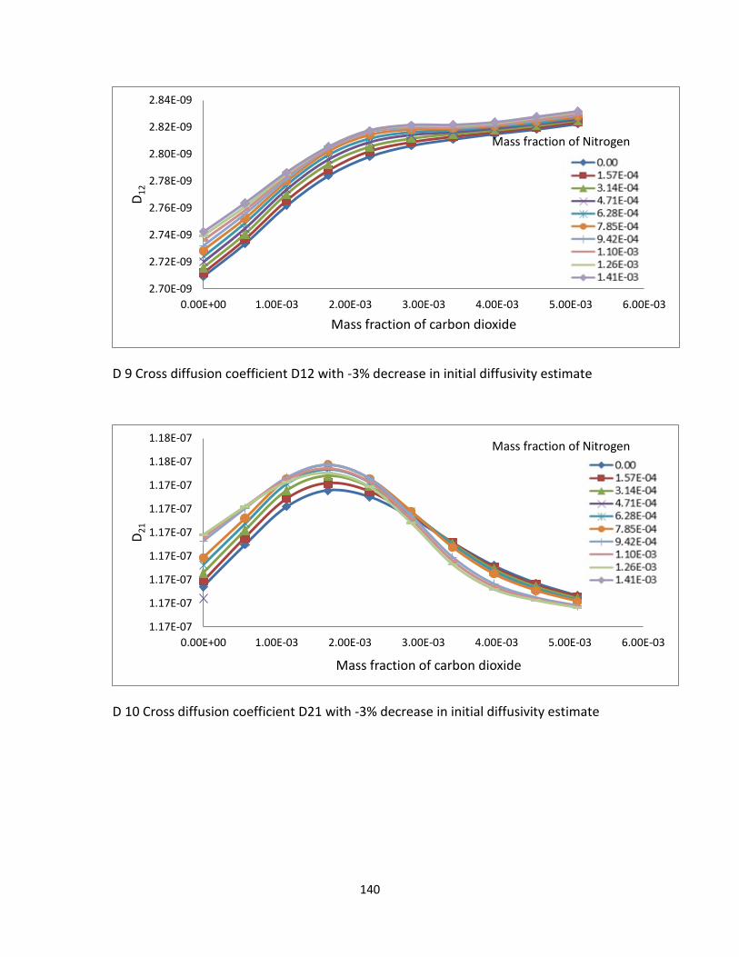
140
D 9 Cross diffusion coefficient D12 with -3% decrease in initial diffusivity estimate
D 10 Cross diffusion coefficient D21 with -3% decrease in initial diffusivity estimate
2.70E-09
2.72E-09
2.74E-09
2.76E-09
2.78E-09
2.80E-09
2.82E-09
2.84E-09
0.00E+00 1.00E-03 2.00E-03 3.00E-03 4.00E-03 5.00E-03 6.00E-03
D1
2
Mass fraction of carbon dioxide
1.17E-07
1.17E-07
1.17E-07
1.17E-07
1.17E-07
1.17E-07
1.17E-07
1.18E-07
1.18E-07
0.00E+00 1.00E-03 2.00E-03 3.00E-03 4.00E-03 5.00E-03 6.00E-03
D2
1
Mass fraction of carbon dioxide
Mass fraction of Nitrogen
Mass fraction of Nitrogen
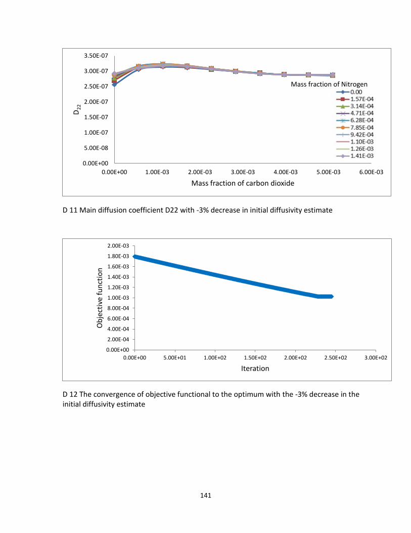
141
D 11 Main diffusion coefficient D22 with -3% decrease in initial diffusivity estimate
D 12 The convergence of objective functional to the optimum with the -3% decrease in the initial diffusivity estimate
0.00E+00
5.00E-08
1.00E-07
1.50E-07
2.00E-07
2.50E-07
3.00E-07
3.50E-07
0.00E+00 1.00E-03 2.00E-03 3.00E-03 4.00E-03 5.00E-03 6.00E-03
D2
2
Mass fraction of carbon dioxide
0.00E+00
2.00E-04
4.00E-04
6.00E-04
8.00E-04
1.00E-03
1.20E-03
1.40E-03
1.60E-03
1.80E-03
2.00E-03
0.00E+00 5.00E+01 1.00E+02 1.50E+02 2.00E+02 2.50E+02 3.00E+02
Ob
ject
ive
fun
ctio
n
Iteration
Mass fraction of Nitrogen
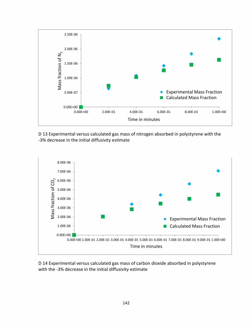
142
D 13 Experimental versus calculated gas mass of nitrogen absorbed in polystyrene with the -3% decrease in the initial diffusivity estimate
D 14 Experimental versus calculated gas mass of carbon dioxide absorbed in polystyrene with the -3% decrease in the initial diffusivity estimate
0.00E+00
5.00E-07
1.00E-06
1.50E-06
2.00E-06
2.50E-06
0.00E+00 2.00E-01 4.00E-01 6.00E-01 8.00E-01 1.00E+00
Mas
s fr
acti
on
of
N2
Time in minutes
Experimental Mass FractionCalculated Mass Fraction
0.00E+00
1.00E-06
2.00E-06
3.00E-06
4.00E-06
5.00E-06
6.00E-06
7.00E-06
8.00E-06
0.00E+00 1.00E-01 2.00E-01 3.00E-01 4.00E-01 5.00E-01 6.00E-01 7.00E-01 8.00E-01 9.00E-01 1.00E+00
Mas
s fr
acti
on
of
CO
2
Time in minutes
Experimental Mass Fraction
Calculated Mass Fraction

143