an introduction to differential evolution · 2004-11-25 · why use differential evolution? •...
TRANSCRIPT
An Introduction to Differential Evolution
Kelly Fleetwood

Synopsis
• Introduction
• Basic Algorithm
• Example
• Performance
• Applications
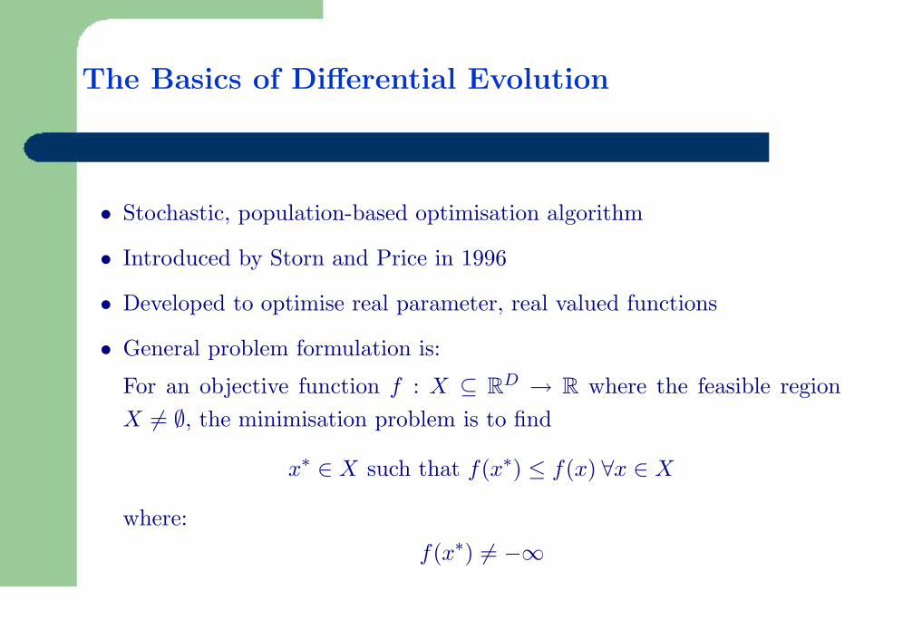
The Basics of Differential Evolution
• Stochastic, population-based optimisation algorithm
• Introduced by Storn and Price in 1996
• Developed to optimise real parameter, real valued functions
• General problem formulation is:
For an objective function f : X ⊆ RD → R where the feasible regionX 6= ∅, the minimisation problem is to find
x∗ ∈ X such that f(x∗) ≤ f(x) ∀x ∈ X
where:f(x∗) 6= −∞
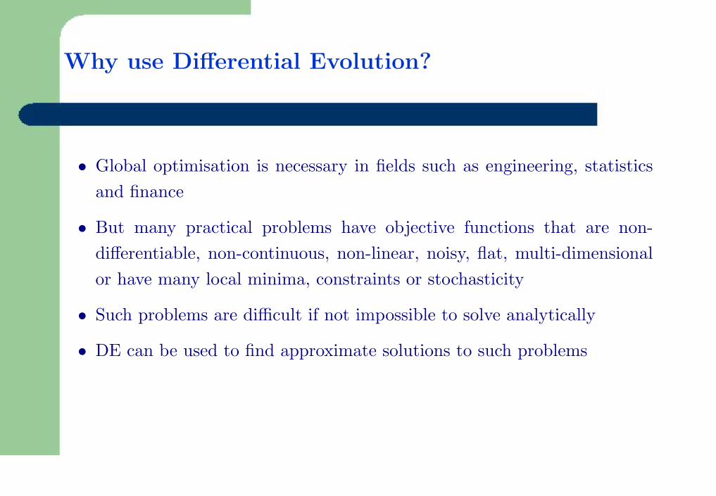
Why use Differential Evolution?
• Global optimisation is necessary in fields such as engineering, statisticsand finance
• But many practical problems have objective functions that are non-differentiable, non-continuous, non-linear, noisy, flat, multi-dimensionalor have many local minima, constraints or stochasticity
• Such problems are difficult if not impossible to solve analytically
• DE can be used to find approximate solutions to such problems
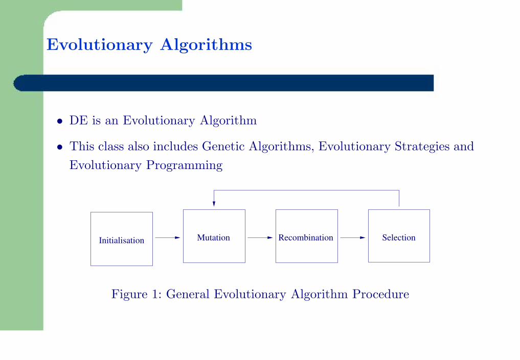
Evolutionary Algorithms
• DE is an Evolutionary Algorithm
• This class also includes Genetic Algorithms, Evolutionary Strategies andEvolutionary Programming
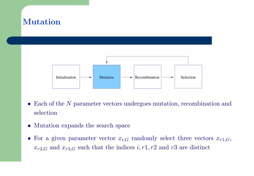
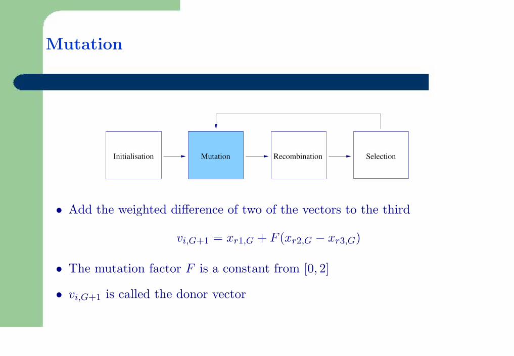
Mutation Recombination SelectionInitialisation
Figure 1: General Evolutionary Algorithm Procedure
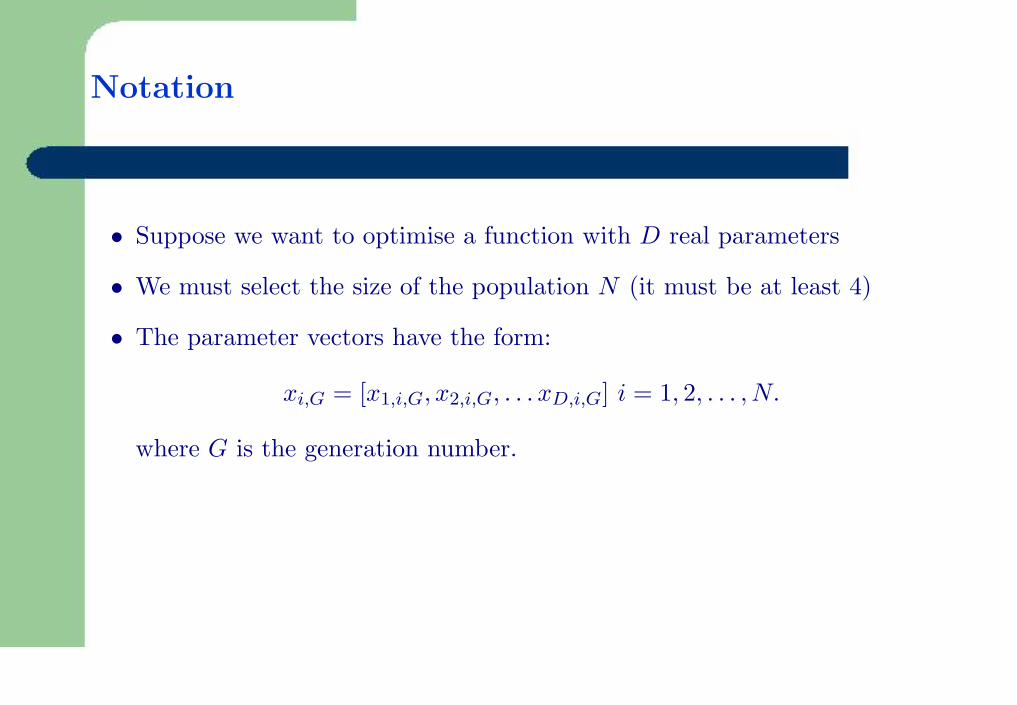
Notation
• Suppose we want to optimise a function with D real parameters
• We must select the size of the population N (it must be at least 4)
• The parameter vectors have the form:
xi,G = [x1,i,G, x2,i,G, . . . xD,i,G] i = 1, 2, . . . , N.
where G is the generation number.
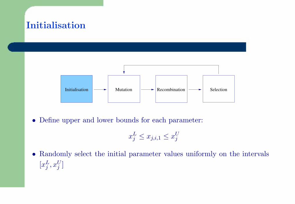
Initialisation
Mutation Recombination SelectionInitialisation
• Define upper and lower bounds for each parameter:
xLj ≤ xj,i,1 ≤ xU
j
• Randomly select the initial parameter values uniformly on the intervals[xL
j , xUj ]
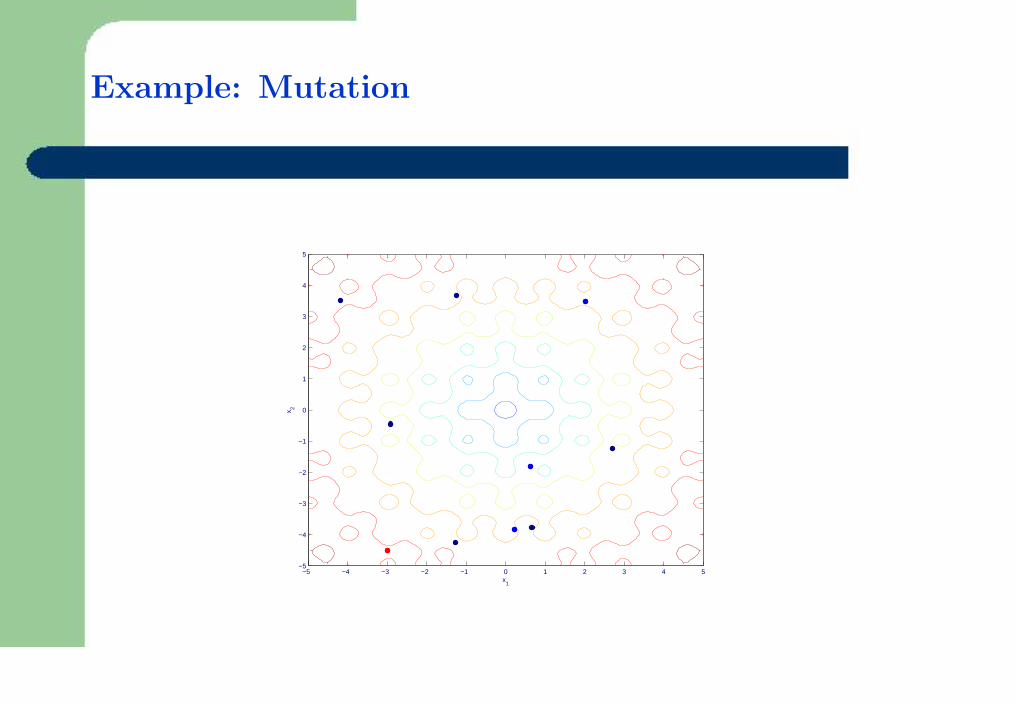
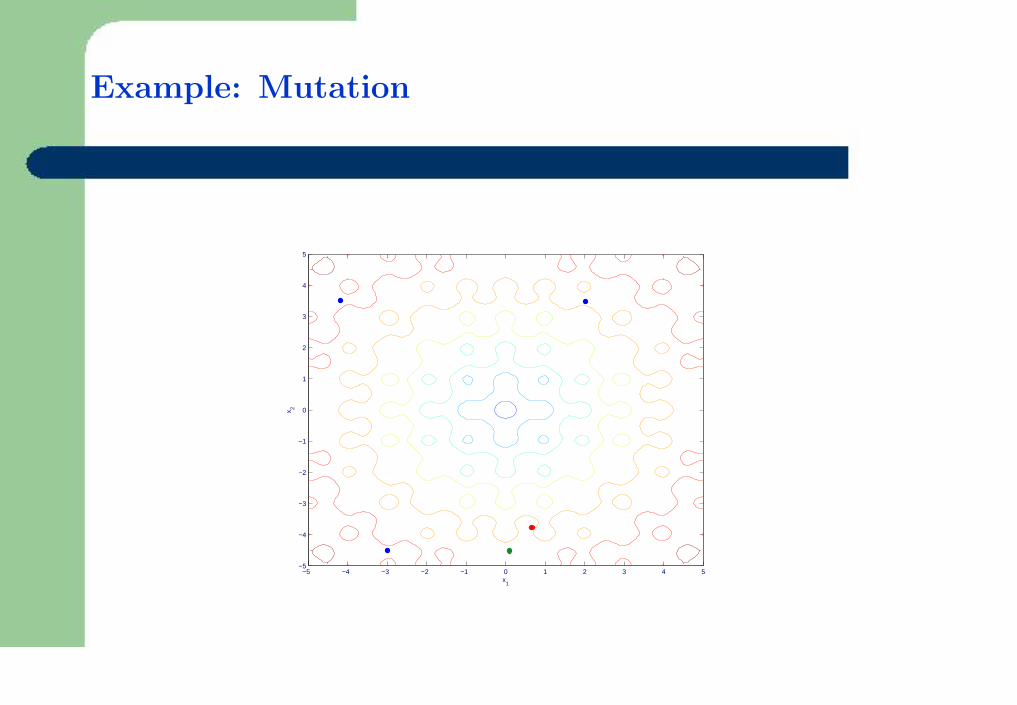
Mutation
Mutation Recombination SelectionInitialisation
• Each of the N parameter vectors undergoes mutation, recombination andselection
• Mutation expands the search space
• For a given parameter vector xi,G randomly select three vectors xr1,G,xr2,G and xr3,G such that the indices i, r1, r2 and r3 are distinct
Mutation
Mutation Recombination SelectionInitialisation
• Add the weighted difference of two of the vectors to the third
vi,G+1 = xr1,G + F (xr2,G − xr3,G)
• The mutation factor F is a constant from [0, 2]
• vi,G+1 is called the donor vector
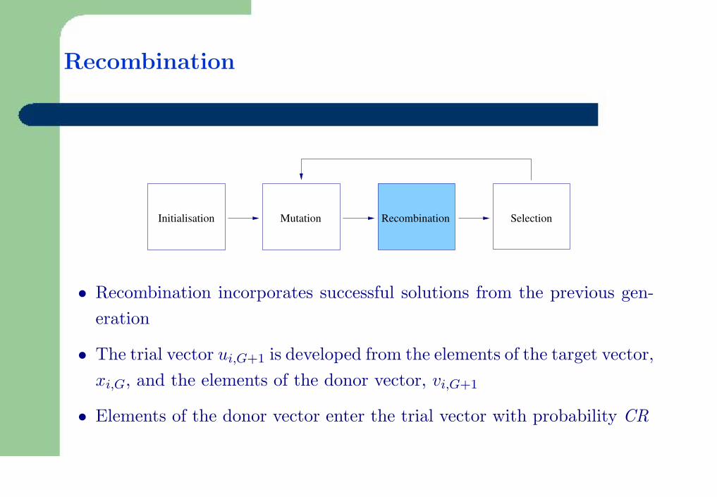
Recombination
Mutation Recombination SelectionInitialisation
• Recombination incorporates successful solutions from the previous gen-eration
• The trial vector ui,G+1 is developed from the elements of the target vector,xi,G, and the elements of the donor vector, vi,G+1
• Elements of the donor vector enter the trial vector with probability CR
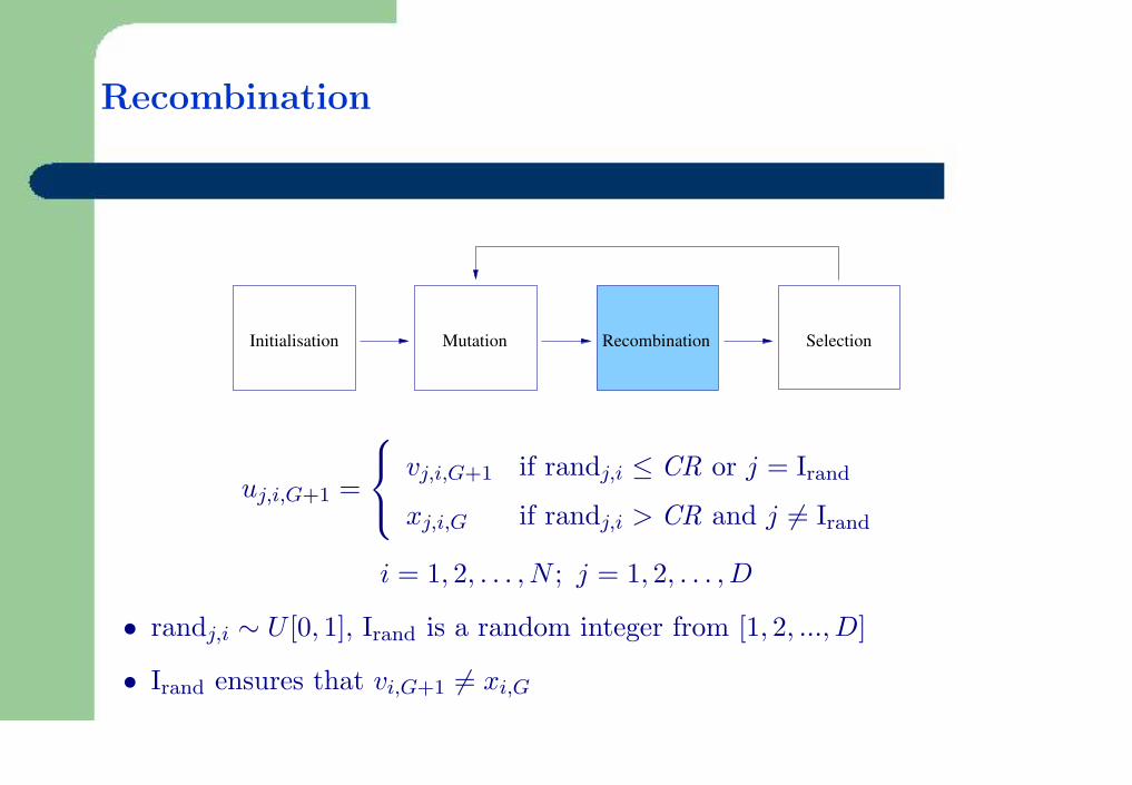
Recombination
Mutation Recombination SelectionInitialisation
uj,i,G+1 =
vj,i,G+1 if randj,i ≤ CR or j = Irand
xj,i,G if randj,i > CR and j 6= Irand
i = 1, 2, . . . , N ; j = 1, 2, . . . , D
• randj,i ∼ U [0, 1], Irand is a random integer from [1, 2, ..., D]
• Irand ensures that vi,G+1 6= xi,G

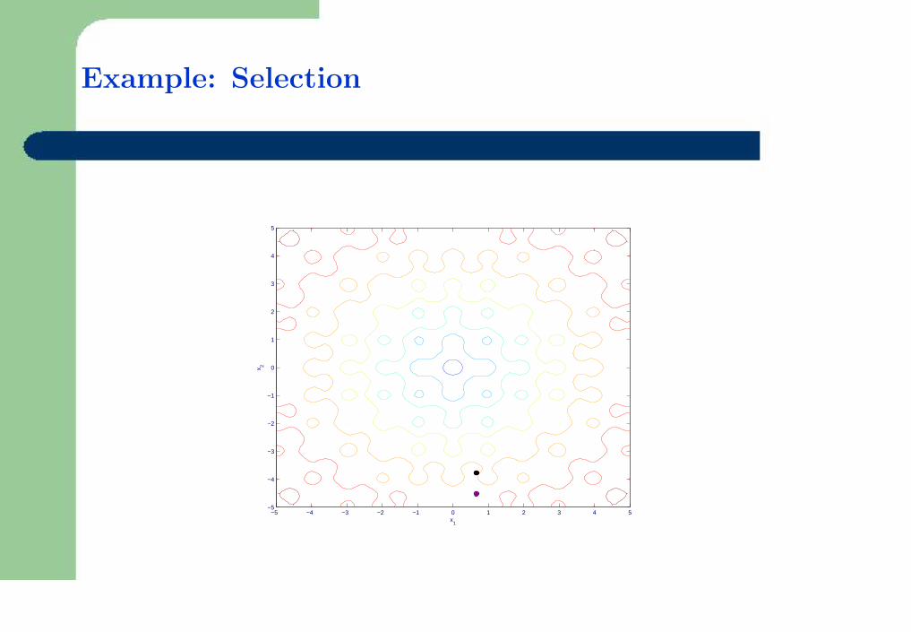
Selection
Mutation Recombination SelectionInitialisation
• The target vector xi,G is compared with the trial vector vi,G+1 and theone with the lowest function value is admitted to the next generation
xi,G+1 =
ui,G+1 if f(ui,G+1) ≤ f(xi,G)
xi,G otherwisei = 1, 2, . . . , N
• Mutation, recombination and selection continue until some stopping cri-terion is reached
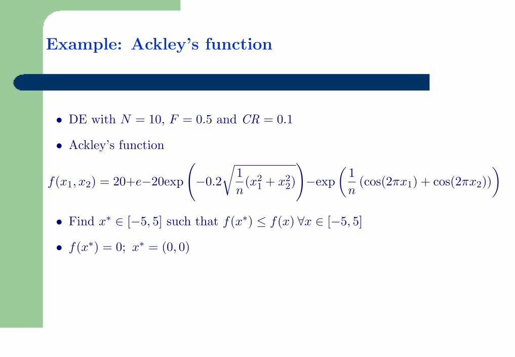
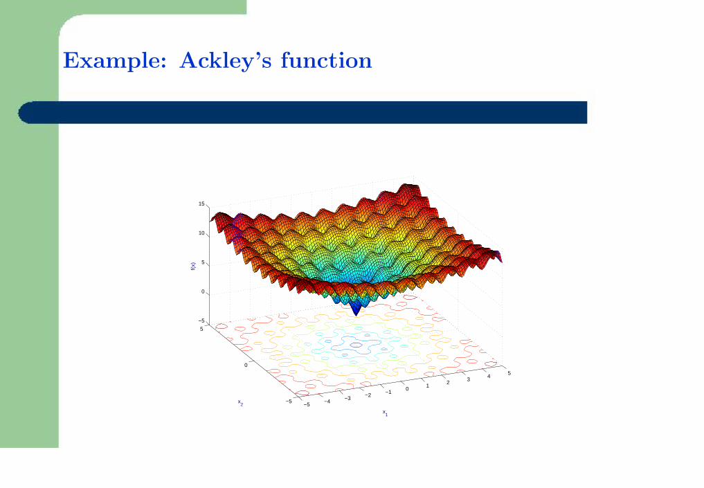
Example: Ackley’s function
• DE with N = 10, F = 0.5 and CR = 0.1
• Ackley’s function
f(x1, x2) = 20+e−20exp
(−0.2
√1n
(x21 + x2
2)
)−exp
(1n
(cos(2πx1) + cos(2πx2)))
• Find x∗ ∈ [−5, 5] such that f(x∗) ≤ f(x) ∀x ∈ [−5, 5]
• f(x∗) = 0; x∗ = (0, 0)
Example: Ackley’s function
−5−4
−3−2 −1
01
23
4 5
−5
0
5
−5
0
5
10
15
x1
x2
f(x)
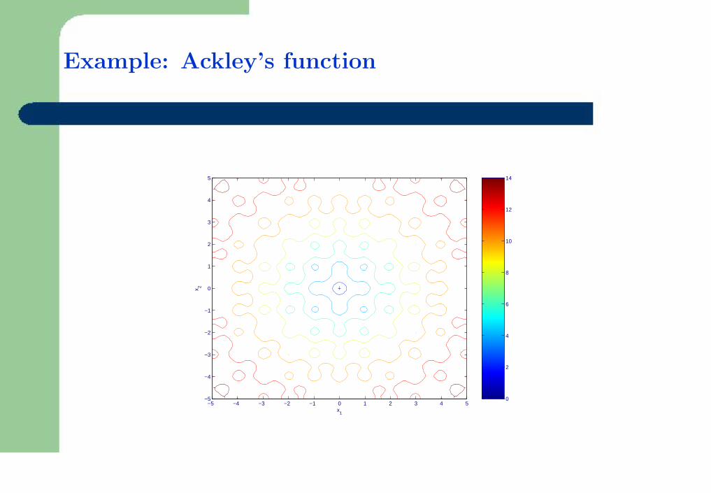
Example: Ackley’s function
−5 −4 −3 −2 −1 0 1 2 3 4 5−5
−4
−3
−2
−1
0
1
2
3
4
5
x1
x 2
0
2
4
6
8
10
12
14

Example: Initialisation
−5 −4 −3 −2 −1 0 1 2 3 4 5−5
−4
−3
−2
−1
0
1
2
3
4
5
x1
x 2

Example: Mutation
−5 −4 −3 −2 −1 0 1 2 3 4 5−5
−4
−3
−2
−1
0
1
2
3
4
5
x1
x 2
Example: Mutation
−5 −4 −3 −2 −1 0 1 2 3 4 5−5
−4
−3
−2
−1
0
1
2
3
4
5
x1
x 2

Example: Mutation
−5 −4 −3 −2 −1 0 1 2 3 4 5−5
−4
−3
−2
−1
0
1
2
3
4
5
x1
x 2

Example: Mutation
−5 −4 −3 −2 −1 0 1 2 3 4 5−5
−4
−3
−2
−1
0
1
2
3
4
5
x1
x 2

Example: Mutation
−5 −4 −3 −2 −1 0 1 2 3 4 5−5
−4
−3
−2
−1
0
1
2
3
4
5
x1
x 2

Example: Recombination
−5 −4 −3 −2 −1 0 1 2 3 4 5−5
−4
−3
−2
−1
0
1
2
3
4
5
x1
x 2

Example: Selection
−5 −4 −3 −2 −1 0 1 2 3 4 5−5
−4
−3
−2
−1
0
1
2
3
4
5
x1
x 2

Example: Selection
−5 −4 −3 −2 −1 0 1 2 3 4 5−5
−4
−3
−2
−1
0
1
2
3
4
5
x1
x 2

Example: Selection
−5 −4 −3 −2 −1 0 1 2 3 4 5−5
−4
−3
−2
−1
0
1
2
3
4
5
x1
x 2

Example: Mutation
−5 −4 −3 −2 −1 0 1 2 3 4 5−5
−4
−3
−2
−1
0
1
2
3
4
5
x1
x 2

Example: Mutation
−5 −4 −3 −2 −1 0 1 2 3 4 5−5
−4
−3
−2
−1
0
1
2
3
4
5
x1
x 2

Example: Mutation
−5 −4 −3 −2 −1 0 1 2 3 4 5−5
−4
−3
−2
−1
0
1
2
3
4
5
x1
x 2
Example: Mutation
−5 −4 −3 −2 −1 0 1 2 3 4 5−5
−4
−3
−2
−1
0
1
2
3
4
5
x1
x 2

Example: Mutation
−5 −4 −3 −2 −1 0 1 2 3 4 5−5
−4
−3
−2
−1
0
1
2
3
4
5
x1
x 2

Example: Recombination
−5 −4 −3 −2 −1 0 1 2 3 4 5−5
−4
−3
−2
−1
0
1
2
3
4
5
x1
x 2

Example: Recombination
−5 −4 −3 −2 −1 0 1 2 3 4 5−5
−4
−3
−2
−1
0
1
2
3
4
5
x1
x 2
Example: Selection
−5 −4 −3 −2 −1 0 1 2 3 4 5−5
−4
−3
−2
−1
0
1
2
3
4
5
x1
x 2

Example: Selection
−5 −4 −3 −2 −1 0 1 2 3 4 5−5
−4
−3
−2
−1
0
1
2
3
4
5
x1
x 2
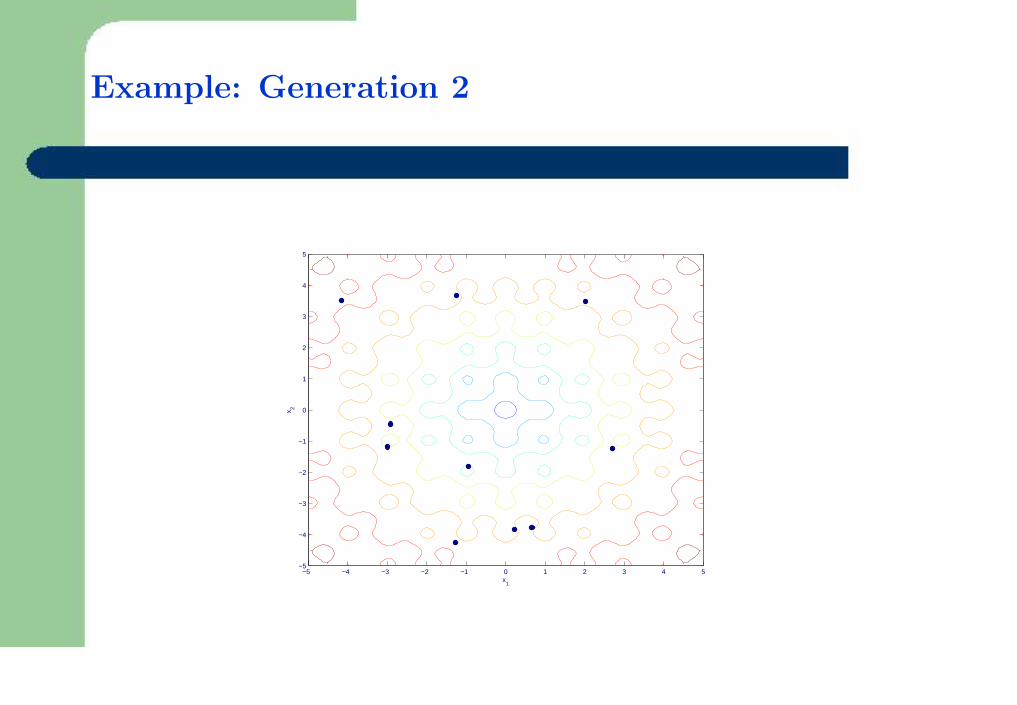
Example: Generation 2
−5 −4 −3 −2 −1 0 1 2 3 4 5−5
−4
−3
−2
−1
0
1
2
3
4
5
x1
x 2

Example: Generation 1
−5 −4 −3 −2 −1 0 1 2 3 4 5−5
−4
−3
−2
−1
0
1
2
3
4
5
x1
x 2
Example: Movie
• Thirty generations of DE
• N = 10, F = 0.5 and CR = 0.1
• Ackley’s function
Performance
• There is no proof of convergence for DE
• However it has been shown to be effective on a large range of classicoptimisation problems
• In a comparison by Storn and Price in 1997 DE was more efficient thansimulated annealing and genetic algorithms
• Ali and Torn (2004) found that DE was both more accurate and moreefficient than controlled random search and another genetic algorithm
• In 2004 Lampinen and Storn demonstrated that DE was more accu-rate than several other optimisation methods including four genetic al-gorithms, simulated annealing and evolutionary programming
Recent Applications
• Design of digital filters
• Optimisation of strategies for checkers
• Maximisation of profit in a model of a beef property
• Optimisation of fermentation of alcohol
Further Reading
• Price, K.V. (1999), ‘An Introduction to Differential Evolution’ in Corne,D., Dorigo, M. and Glover, F. (eds), New Ideas in Optimization, McGraw-Hill, London.
• Storn, R. and Price, K. (1997), ‘Differential Evolution - A Simple and Effi-cient Heuristic for Global Optimization over Continuous Spaces’, Journalof Global Optimization, 11, pp. 341–359.