Transportation Research Part C 38 (2014) 73–84

Contents lists available at ScienceDirect

Transportation Research Part C

journal homepage: www.elsevier .com/locate / t rc

An intermodal freight transport system for optimal supply chainlogistics

0968-090X/$ - see front matter � 2013 Elsevier Ltd. All rights reserved.http://dx.doi.org/10.1016/j.trc.2013.10.012

⇑ Corresponding authors.E-mail addresses: talluri@msu.edu, mkt09@hotmail.com (S. Talluri).

Arnab Bhattacharya a, Sai Anjani Kumar a, M.K Tiwari a,⇑, S. Talluri b,⇑a Department of Industrial Engineering and Management, Indian Institute of Technology, Kharagpur 721302, Indiab Department of Supply Chain Management, Broad School of Business, Michigan State University, 351 N. Business Complex, East Lansing, MI 48824, United States

a r t i c l e i n f o

Article history:Received 14 May 2012Received in revised form 31 October 2013Accepted 31 October 2013

Keywords:Spatio-temporal data miningIntermodal transportSupport vector machinesMixed integer programming

a b s t r a c t

Complexity in transport networks evokes the need for instant response to the changingdynamics and uncertainties in the upstream operations, where multiple modes of transportare often available, but rarely used in conjunction. This paper proposes a model for strate-gic transport planning involving a network wide intermodal transport system. The systemdetermines the spatio-temporal states of road based freight networks (unimodal) andfuture traffic flow in definite time intervals. This information is processed to devise effi-cient scheduling plans by coordinating and connecting existing rail transport schedulesto road based freight systems (intermodal). The traffic flow estimation is performed by ker-nel based support vector mechanisms while mixed integer programming (MIP) is used tooptimize schedules for intermodal transport network by considering various costs andadditional capacity constraints. The model has been successfully applied to an existing FastMoving Consumer Goods (FMCG) distribution network in India with encouraging results.

� 2013 Elsevier Ltd. All rights reserved.

1. Introduction

The growing interest in collaborative logistics is fuelled by increasing pressure on companies to operate more efficientlyand enhance the productivity of their supply chains. Transportation and logistics management is fast becoming one of thekey components of the entire supply chain valuation for many organizations. Due to increasing globalization in recent dec-ades, especially in emerging economies, the importance of logistics management has been on the rise. Traditionally, shippersand carriers have focused their attention on minimizing their own costs to increase profitability, but more recently focus hasshifted towards system wide cost reduction to increase profitability of the entire logistics chain. A key component of a logis-tics chain is the transportation system network. The costs associated with transportation amount to around one third of thetotal logistics costs which necessitates effective and cost efficient transport coordination mechanisms for managing complexnetworks involving shipments from manufacturing plants through intermediate distribution centers to customer retaillocations.

In many developing economies, majority of the freight transport is undertaken by road based vehicles while rail andwater based services remain either largely unutilized or highly disorganized in their functioning and coordination. Roadbased freight transport has increased significantly over the past few decades in the distribution channels. This rapid increasehas led to massive overuse of the road networks without much improvement in the existing infrastructure resulting in var-ious externalities like traffic congestion, increased energy consumption and negative environmental impact. Road capacities,especially outside urban areas, are still inadequate, and several road segments are in inferior condition in the developingcountries. In addition, the port and operational transshipment terminals are few in number with low levels of service due

74 A. Bhattacharya et al. / Transportation Research Part C 38 (2014) 73–84

to lack of berths, supporting equipment and maintenance. In order to address these issues, we focus on an efficient organi-zation of intermodal transport system which can alleviate these externalities based on the current status of the distributionchannel of the supply chain network. Our approach in this paper is aimed at taking advantage of intermodal transport wher-ever possible in a network heavily dependent on unimodal transport.

According to Mahoney (1986), ‘‘Intermodality’’ is the movement of freight via two or more dissimilar modes of transpor-tation. Hayuth (1987) defines it as the movement of cargo from shipper to consignee by at least two different modes of trans-port under a single rate, through-billing, and through liability. In general, research in the area of intermodal transportsystems not only assists in developing effective transport networks, but also contributes to reducing negative impact onenvironment and energy consumption. In developing countries such a system will drastically improve the utilization oftransport resources and services, leading to better scheduling and delivery with lower logistics costs and higher levels ofefficiency.

In this paper, an integrated intermodal freight transport system is developed for an established FMCG distribution net-work in India. The system first analyzes the traffic status of the road based freight vehicles in various operational zones (spa-tial clusters) of the network at different time intervals. The system then computes a congestion index for that spatial clusterwhich is then utilized for any decision to engage other transport modes in the network, such as rail and water links whereveravailable. The decision for engaging another mode of transport is based on the results of optimizing the total costs involvedin the intermodal strategy. In this model, rail is chosen as the primary alternative to road due to certain advantages that in-clude better connectivity, regulated schedules, diversified distribution channel and faster delivery time within acceptabletransport cost limits. A single alternate also reduces the complexity and is a fair representation of the networks in mostdeveloping countries. However, our approach can easily be extended to other available transport modes with time-spacerepresentations. The intermodal train service routes are determined under specific time slots when the train services areoffered.

The rest of the paper is organized as follows. The next section reviews literature relating to similar work conducted in thefields of spatio-temporal mining and intermodal transport optimization. We then describe the general methodology in de-tail. The following section introduces the modeling approach utilized and discusses the details of problem formulation. Theresults are presented and discussed next, followed by conclusions and future extensions in this area.

2. Literature review

In this section, related work in spatio-temporal traffic flow prediction and intermodal transport optimization is discussedwhich sets the stage for the problem addressed in this paper. From a methodology standpoint, majority of the work in theseareas focuses on advanced predictive analytics using non-linear, non-parametric regressive models and integer program-ming for combinatorial optimization.

2.1. Spatio-temporal short-term traffic flow prediction

Since the 1970s, univariate time series models have been widely used for traffic flow prediction, especially Box–Jenkinsautoregressive integrated moving average (ARIMA) models (Hamed et al., 1995). Subsequently, ARIMA and exponentialsmoothing (ES) models, such as Holt’s–Winter’s approach, have been used for comparison purposes whenever a new fore-casting model for short-term traffic is proposed (Park et al., 1998). Over the past decade, Neural Network (NN) models havebeen extensively used in the field of transportation engineering. In addition to flow, other traffic parameters including speed(Ishak et al., 2003) and occupancy (Zhang, 2000) have been predicted in real-time by NN models. Several other techniqueshave been applied to predict real-time traffic flow. Some of these include multivariate state space time series (Stathopoulosand Karlaftis, 2003) multivariate non-parametric regression (Clark, 2003; Smith and Demetsky, 1996), dynamic generalizedlinear models (Lan and Miaou, 1999), Hybrid fuzzy rule based system approach (Dimitriou et al., 2008) and Kalman filteringmodels (Okutani and Stephanedes, 1984). Lin (2001) proposed a forecasting model based on the Gaussian maximum likeli-hood (GML) estimation method to perform one step ahead forecasts using 5-min traffic flow data. Lin’s methodology usedboth current and historical data traffic in an integrated manner. Probabilistic Principal Component Analysis has been effec-tively employed using intra-day trend of traffic flow series. This largely removes the issue of missing data while keeping pre-diction errors relatively low (Chen et al., 2012). Better results have been observed for advanced genetic algorithm basedmultilayered optimization strategy for neural networks (Vlahogianni et al., 2005). Historic aggregated data from large dat-abases of neighboring stationary detectors and congestion analysis was used to predict traffic flow instabilities (Treiber andKesting, 2012). Recently, support vector regression (SVR) is being widely applied to predict traffic parameters such as traveltime (Wu et al., 2004). The major advantage of SVR is that it avoids over-fitting and allows for a faster training process thanother algorithms for multi-dimensional data.

A number of incident detection algorithms have been developed over the past three decades. One of the most popularalgorithms is the California Algorithm (Payne and Tignor, 1978). This algorithm is based on the logical assumption that atraffic incident increases the traffic occupancy at the upstream portions of the incident and significantly decreases the trafficoccupancy downstream of the incident. However, majority of these algorithms are not reliable in differentiating betweenrecurrent and non-recurrent congestion events. The Minnesota Algorithm (Chassiakos and Stephanedes, 1993) attempts

A. Bhattacharya et al. / Transportation Research Part C 38 (2014) 73–84 75

to minimize false alarms and missed incidents by filtering out the effects of high frequency random fluctuations in trafficflow using averaging occupancy measurements over contiguous short-term intervals.

2.2. Optimization of intermodal transport network

Several contributions exist on train routing and scheduling and on applied service network design for train operations.Gorman (1998) focus on service network design models with schedules for CSX transportation and Santa Fe Railways,respectively. Southworth and Peterson (2000) shed light on GIS based intermodal freight network modeling with cost effec-tive network maintenance and traffic route selection for various modes. Yano and Newman (2001) present a dynamic mod-eling approach to schedule departures of freight and trains to and from a single terminal. Newman and Yano (2000) proposeda train routing model which includes schedules. However, freight demand is modeled to originate and destined to rail ter-minals, thus drayage moves are not considered. Gorman (1998) developed a linear mixed integer programming (MIP) modelfor train scheduling with limited terminal operations. The MIP models determine the optimal scheduling on a space-timerepresentation of a network for two types of trains including the train make-ups and empty wagon repositioning problem.Wong et al. (2008) developed a MIP-model to minimize total transfer time for smooth flow and obtained optimal timetableusing a heuristic. Yamada et al. (2009) detailed a bi-level programming to obtain multimodal multiuser flow and a benefit-cost ratio (BCR) is considered as objective function to identify best combination for network effectiveness. The related resultsare obtained using genetic algorithm and Tabu search methods. Caprara et al. (2011) developed a column generation meth-odology to solve integer linear programming (ILP) model for obtaining efficient routes considering service level of goods.Majority of the models in the literature obtained either optimal travel route using different modes or obtained schedulesfor usage of different modes. Traffic congestion along different routes is an important issue, which has not been integratedinto these approaches working on intermodal freight. This paper develops an integrated modeling structure by which a tra-vel manager will be able to decide whether to consider a unimodal or intermodal strategy based on cost-time tradeoff for acomplex distributions network.

3. Methodology

The methodology has two distinct steps which are integrated and implemented as a part of the overall intermodal trans-port architecture for the distribution channel. We now discuss each of these steps below.

The first step of the model involves finding the degree of traffic congestion of the road based freight services in the logis-tics network of our supply chain. The main objective of this part of the study is to perform short-term freeway traffic flowpredictions under normal or abnormal events. As stated earlier, in developing economies road based services are the mainmode of transport for shipment of goods from the manufacturing or distribution centers to the customer locations. For a net-work that is heavily dependent on road based services, it becomes critical to assess the traffic congestion status at regularintervals, which becomes critical in sectors where the road infrastructure is inadequate to handle the large flow of goodsespecially into metropolitan and industrial centers. This vehicle tracking and congestion analysis measures are further usedfor determining the need for intermodal transport that includes rail or water in case of high congestion in the road network,which results in cost savings and better delivery turnaround. The vehicle data have both space (spatial) and time (temporal)dimensions, which are ideal for dynamic response of the system. The analysis is important in developing a strategic decisionmaking mechanism as part of an optimal logistics chain with defined scheduling and delivery timelines.

Traffic congestion is evaluated based on the spatio-temporal data mining process to detect incidents for definite timestamps (e.g. each day of the week, each hour of the day etc.) based on quantitative metrics such as velocity, volume of occu-pancy, and identifying outliers in each spatial cluster by comparing the traffic data at a particular time interval with the his-torical models at the same time slot. The outliers, with congestion index above a threshold value, serve as alarms. Theyindicate high congestion level at that time interval(s) for the given spatial cluster, which is the district or locality observedat that instant of time. The data is acquired through GIS (Geographical Information Systems) or freeway detectors positionedon the road network at regular intervals or mileposts from different spatial clusters in the network.

The short-term traffic flow analysis is followed by determination of the future predicted pattern of the above short-termtraffic movement. Accurate prediction of future movements in short time frames gives the schedule manager important in-sights regarding the congestion in the network and the ability to make decisions for the future based on the patterns appear-ing on a daily basis. Work in online prediction (Zeng et al., 2008) for short-term flow has shown that results from SVR arebetter than competing algorithms such as NN and other non-parametric models. So, in our model, we use SVR for short-termtraffic forecasting in each cluster. The prediction gives a detailed network occupancy forecast for the definite timestampsassociated with the system. The second step deals with the problem of optimization of an intermodal network consistingof road and rail as the two primary means of transport. The decision to employ rail for the distribution channel is basedon the traffic spatio-temporal congestion analysis and traffic congestion forecasts in the road network clusters. High conges-tion with high degree of movement and occupancy in the forecast evokes the need to shift to rail. The model considers thetime scheduling and synchronization of the train network and the terminal operations to minimize the transit times asso-ciated. The improvement in operations is evaluated based on intermodal trip parameters and comparing it to long-haultrucking.

76 A. Bhattacharya et al. / Transportation Research Part C 38 (2014) 73–84

Fig. 1 depicts a small cluster of the logistics network of a consumer goods company consisting of four containers withdifferent customer origins and destinations that can share the railway freight services. There are three railway terminals.The total transit time for the intermodal chain will be the sum of the drayage transportation times, loading and unloadingtimes at transshipment terminals, rail connection delays, rail transportation time and transportation delays in the drayagemovements. This sum of the operations times has to be competitive and more efficient than direct long haul road based ser-vices for the intermodal transport to be employed in favor of road. The focus is to reduce the costs associated with these timedelays along with the operation costs. We assume that trains always run with the same number of wagons with an upperbound for maximum freight capacity. Transshipment operations at the terminals are considered. Also, the train terminalscan hold inventory for short periods of time. There is a limitation on the number of tracks available at the railway terminals,and hence the number of trains available for operations at any given time. As a result, schedule synchronization becomesvery important especially as the decision for switching over to intermodal transport is a completely random event basedon the congestion analysis of the road network. There is a tradeoff between high frequency of trains resulting in reducedtransit times and high operational and handling costs. A MIP approach is utilized to model the problem to capture this trade-off between operation and time related costs.

4. Modeling approach

4.1. Traffic data analysis

Spatio-Temporal databases are maintained in the network chain to store current traffic information, color coded trafficmaps and information of each individual transport vehicle (of any mode) in the distribution network. GIS and detectorson tracking stations are primarily employed to store these data. The route planning problem will be dependent on trafficinformation in the path ahead and the predicted congestion for a series of time intervals. A methodology is devised to detectthe recurrent and non-recurrent congestions in the road network. Both the spatial and temporal information is used for thetraffic analysis (unlike traditional methods which use either spatial or temporal information). One of the first and most pop-ular algorithms is the California algorithm (Payne and Tignor, 1978) which relates traffic occupancy to incident detectionusing a spatio-temporal dataset and decision tree modeling. Our analysis extends the original methodology while exploringa support vector mechanism for congestion prediction. It involves the following steps:

� Data preparation and categorization: The database is scanned to identify noisy data, which are removed. Records of thespecial incidents (eg. Holidays, Blockades) are labeled and data is categorized for different time intervals (for example,hour, day, week, month, etc.)� Model generation: Temporary traffic models are developed based on the mean value of a variable that represents or acts as

a proxy to congestion, such as speed or volume occupancy. In our model speed is used as the metric for congestion anal-ysis. A specific lower limit threshold distance d_low is determined. This is compared to the vector distance between his-torical data and the observed data with distances greater than d_low eliminated from the model.� Congestion analysis: The congestion evaluation process for the road traffic data is implemented in this step. Traffic data is

updated for distinct timestamps and cleaned in runtime. Congestion detection is performed by calculating the Mahalan-obis distance between real time data and the corresponding time slot in the traffic model. If the distance calculated isgreater than a specified threshold d_high, it signals a certain incident causing congestion in the area of analysis. Mahalan-obis distance between vector ~x (real time vehicle data) from a group of values with mean ~l (calculated from historicaldata) is calculated using expression (1) below:

Fig. 1. Intermodal transport chain.

A. Bhattacharya et al. / Transportation Research Part C 38 (2014) 73–84 77

dð~X; ~lÞ ¼ffiffiffiffiffiffiffiffiffiffiffiffiffiffiffiffiffiffiffiffiffiffiffiffiffiffiffiffiffiffiffiffiffiffiffiffiffiffiffið~X �~lÞS�1ð~X �~lÞ

q

dð~X; ~lÞ � v2n�1

ð1Þ

It follows the chi-square distribution, where d_low and d_high can be assigned using probability distribution for a certainlevel of confidence (we use 95% and 98% levels).

� Detection level for consecutive timeslots: Det_Lev (similar to a signal level) is time dependent and based on number of inci-dents recorded for consecutive time slots (which in turn determines congestion). For the fixed number of time slots con-sidered, the detection level will increase with each new incident (indicator of congestion) in that particular timestampand decreases when no incident is detected. The detection level function is formulated as given below, which has an inci-dent detection rate l(t).

Det LevðtÞ ¼ Det Levðt � 1Þ þ lðtÞ when congestion is det ectedDet LevðtÞ ¼ De Levðt � 1Þ � lðtÞ when congestion is not det ected

ð2Þ

Once the signal level increases over a certain level (Det_Lev_limit), short-term forecasting of traffic movement for the par-ticular cluster is initiated.� Support vector regression forecasting model: For the given problem, the set of data points (in the specific cluster) where the

signal function exceeds the upper threshold value (Det_Lev(t) > Det_Lev_limit), is analyzed for congestion prediction. Themathematical analysis is provided below, which is calculated for each spatial cluster (Clust_i, i = 1, . . . ,n) in the networkroute.A linear regression function is defined in accordance with SVR theory to find the predicted values.Total number of points in cluster: mSet of points in the network: ðx1; y1Þ; ðx2; y2Þ; . . . ; ðxm; ymÞ

hðxÞ ¼ wTuðxiÞ þ b ð3Þ

We define the above function taking into account: F, a feature space; w, a vector in F; /ðxiÞ, a mapping function whichmaps each xi to a vector in F; e, an insensitive loss function as proposed by Vapnik (1995); it is the maximum error allowedduring training of the dataset; C, penalty cost for deviation during training process; nþi n�i , slack variables corresponding to thesize of the excess deviations; wT w, regularized term controlling the function capacity;

Pðnþi þ n�i Þ, empirical error calculated

from the insensitive loss function.Based on SVR literature, the given optimization problem is solved:

Minimize12

wT wþ CXðnþi þ n�i Þ ð4Þ

Subject toyi �wTUðxiÞ � b 6 eþ nþiwTUðxiÞ þ b� yi 6 eþ n�inþi ; n

�i P 0

ð5Þ

The above problem is solved using the Kuhn Tucker Conditions (KKT) as described in Ma et al. (2003).The prediction can be based on timestamps such as 5 min, 10 min and 15 min. The forecasting involves the following

steps:

Step 1: Use a prediction horizon of one time stamp for a given time series d(t), t = 1, 2, 3,. . .. and prediction origin Or, timeat which the prediction process starts.

Step 2: Construct a set of training samples train(Or, B) from d(t), where train(Or, B) = {D(t), y(t), t = B,. . .Or} and D(t) = [{d(t),. . .d(t � B + 1)}]0, y(t) = d(t + 1) and B is dimension of the training set.

Step 3: Train a predictor Pr(train (Or, B), D) from the training set train(Or, B) and predict d(O + 1) using d(O + 1) = Pr(trai-n(Or, B), D(O))0.

Step 4: Prediction origin is updated and the process is repeated. Results are processed using different kernel functionssuch as Polynomial kernels.

Step 5: Prediction Performance is calculated by mean absolute percent error (MAPE) and Sensitivity (S).

MAPEð%Þ ¼ 1n

Xðj yi � yi j =yiÞ � 100

S ¼ ðnumber of correct prediction=total predictionÞ � 100ð6Þ

The predicted values are then subjected to the detection analysis for the consecutive timeslots of the prediction horizonby comparing the Mahalanobis distance between the predicted values and the historical traffic model, and followed by find-ing the corresponding detection level. We compile the results of all the spatial clusters and find the congestion index for eachroute in the network.

78 A. Bhattacharya et al. / Transportation Research Part C 38 (2014) 73–84

4.2. Intermodal transport optimization

The traffic flow prediction analysis forecasts the congestion in future timeslots in the network. This becomes the basis fordevising intermodal strategy in the particular routes where congestion is likely. The intermodal transport module will thenbe activated to consider the possibility of using other transport modes if available for delivery schedule starting from thoseparticular sectors. The objective of the model is to capture the trade-off between operational costs and the value of time costincurred in the freight transit times and minimize the sum of the two. The characteristics of the model are given below.

4.2.1. Network structure and modal corridorModal corridors are defined to make the scheduling process easily comprehendible. These corridors can be defined for any

mode with limited infrastructure in terms of deployment and having structured scheduling pattern. Each rail corridor has anassociated fixed cost which includes the crew operating cost, maintenance and depreciation cost or leasing cost of locomo-tives and wagons, and fuel costs. In our model, train corridors are considered, with predefined time-dependent paths on thephysical infrastructure. A corridor allows only one train (or any mode for which the corridor is defined) to run at a time. Thenetwork is composed of arcs between the terminals which represent the routing connections between the terminals, and thearcs between the terminals and the customer nodes as the possible drayage movements (as shown in Fig. 2). The network ismodeled as a spatio-temporal network which takes into account the scheduling aspect of the service.

4.2.2. Customer dependent freight demandFreight demand on the service network has a certain level of uncertainty because of lack of detailed knowledge of cus-

tomer demand. The network also has correlations with demand levels, as the train frequency increases with demand levels.The demand is assumed to arrive from large customer zones with some quantitative estimate of demand potential.

4.2.3. Spatial clusters of customer zones, terminal operations, and drayage movementsCustomers are grouped into different customer zones (spatial clusters) associated with one or more railway terminals.

Drayage movements require at least one truck for each container. The model assumes that transportation costs are equalfor all customers in a customer zone and is commodity indifferent. Transshipment becomes critical in terminal operations.Terminals are also capable of holding inventory, until they are transported to the customer nodes via drayage movements.Variable vehicle transfer/transshipment costs are attached to each departing train corridor arc and departing drayage arcwith additional cost of loading and unloading.

4.2.4. Mathematical formulationIn this section, we present the mathematical formulation for the MIP optimization model. It is an arc flow based model.

Following notion is used for our problem:

}: set of all customer zones.�hz: set of customer zone nodes for each customer zone z 2 }.

Fig. 2. Intermodal transport network.

A. Bhattacharya et al. / Transportation Research Part C 38 (2014) 73–84 79

Sz2}�hz: union of all customer zone nodes for each customer zone z in the network.

S: set of all terminals in the network.�hs: set of terminal nodes for each terminal s 2 S.S

s2d�hs: union of all terminal nodes in network.1: set of commodities that represents demand in the network.oðpÞ: origin (starting) customer zone node of commodity p 2 1.d(p): destination (ending) customer zone node for commodity p 2 1.tck: time of availability of commodity p for each customer zone node k.J: set of modes representing different trains with different number of containers.1m: fði; jÞ j ði; jÞ 2

S�hsg: set of train corridors (arcs) connecting terminal i to j.

�h�s;mðiÞ; �hþs;mðiÞ: inward and outward neighbors of node i from terminal s.

r�: fðk; iÞ j k 2S

�hz; i 2S

�hsg: set of drayage arcs from customer zone z to terminal node s.rþ: fði; kÞ j i 2

S�hs; k 2

S�hzg: set of drayage arcs from terminal node s to customer node z.

�h�z ðiÞ; �hþz ðiÞ: set of inward and outward customer zone nodes in zone z from terminal node i.

�h�s ðzÞ; �hþs ðzÞ: set of outward and inward terminal nodes from terminal s for customer zone z.

4.2.4.1. Notation.

xwi;p: holding amount of commodity p at customer zone node k.

xli;p: amount of commodity p unloaded at terminal node i.

xmi;p: amount of commodity p loaded at terminal node i.

xxi;p: inventory of commodity p at terminal node i to customer node k.

xdþi;h;p: flow of commodity p from customer zone k to terminal node i.

xki;j;m;p: flow of commodity p on train carrier m running between terminals i, j.

yki;j;m ¼

10

�if train carrier m uses terminals (i,j).

4.2.4.2. Decision variables.ti;s: start time associated with terminal at node i.ti;e: end time associated with terminal at node i.tck: transit time of inventory arc from terminal node k.tdþ

ki ðtd�ik Þ: difference between terminal’s and customer zone start (end) times shows the time associated with dryage

movement.tk

ij: transit time of train canal arc(i,j)cx

i : unit cost of inventory arc from terminal node ick

ij ¼ coi þ b:tkij: unit cost train canal arc (i,j), here b is a parameter that accounts for cost associated with the time. The value

of b indicates the additional cost associated with a unit time increment.cdþ

ki ¼ cdþki þ b:tdþ

ki : unit cost of using drayage arcs from customer zone k to terminal node i.cd�

ik ¼ cd�ik þ b:td�

ik : unit cost of using drayage arcs from terminal node i to customer zone k.

The range of the unit costs (given in Table 1) for usage of drayage arcs and the unit train canal costs arise due to the linearrelationship of these costs to tdþ

ki ; td�ik and tk

ij respectively.

wi: inventory capacity limit of terminal node i.ui: handling capacity of terminal node i.vi: train capacity of terminal node i.cl

i : unit cost for unloading arc in terminal node i.cv

i : unit cost for loading arc in terminal node i.f ki;j;m: fixed cost of routing train carrier m on train corridor arc(i,j).

The objective function involves the minimization of fixed train corridor costs and container transit costs as shown in (7)below:

min z ¼Xði;jÞ

Xm2�h

f kijmyk

ijm þXXX

ckijx

kijpm þ

XXcx

i xxip þ

XXcl

i xlip þ

XXcm

i xmip þ

XXcdþ

ki xdþkip

þXX

cd�ik xd�

ikp ð7Þ

The following are the constraints that are utilized for flow conservation:

Table 1Instance attributes.

NodesTotal nodes 350Terminals 140 Load/unloading costTerminal nodes 210

Vehicle transfercost ($)

Handling cost($)

Storage cost ($) Handling capacity(units)

Storage capacity(units)

Train capacity(units)

Ranges 68–88 70–100 15–35 60–110 100 2–4

ArcsNo. of arcs 787Train canal arcs Mode 1 Mode 2 Mode 3

225 109 75203 106 69

Train transfer arcsTrain canal cost ($) Train transfer cost

($)Train canalcost ($)

Train transfercost ($)

Train canal cost ($) Train transfer cost($)

9000–14,000 6500 19,800–27,000 130,000 38,600–50,460 27,000No. of drayage arcs 450

Unit transportation cost ($)Range 78–150

Commodities (units)No. of commodity 100

Low Medium HighCommodity amount range

(units)3–6 5–9 6–12

Total 399 618 798Time horizon 200 h

80 A. Bhattacharya et al. / Transportation Research Part C 38 (2014) 73–84

Constraint 1: Commodity flow balance in customer zones. The outflow, holding and the demand levels at each customerzone needs to be balanced.

xwnz�ðkÞ;p þ akp ¼ xw

kp þXS

�hsþðkÞ

xdþkjp 8k 2 [�hz ð8Þ

Constraint 2: The flow balance constraint for commodities arriving at their destination customer zone. The inflow must besuch that it satisfies the demand.

XS

�hs�ðzÞ

Xk2�hz

xd�ihp ¼ azp 8z 2 } ð9Þ

Constraint 3: The sum of the flow of commodities on arriving train arcs, arriving drayage arcs, and the loading arcs mustbe equal to the sum of the flow on departing train arcs, departing drayage arcs, and the unloading arcs:

Xm

X[�hsmþðiÞ

xkhip þ

Xk2S

�hzþðiÞ

xdþkip þ xl

ip ¼X

m

X[�hsm�ðiÞ

xkijpm þ

Xl2S

�hz�ðiÞ

xd�ilp þ xv

ip ð10Þ

Constraint 4: For each terminal node i, the sum of the inventory flow from the predecessor (inventory level before the startof the time period) and what is unloaded must be equal to the sum of what is loaded plus what is left in inventory:

xxnsþðiÞip þ xl

ip ¼ xxip þ xv

ip ð11Þ

Constraint 5: Inventory level must be lower than the terminal node storage capacity:

Xh2�hsmþðiÞ

ykhim ¼

Xj2�hsm�ðiÞ

ykijm ð12Þ

Constraint 6: The maximum number of commodities that can flow on a corridor is constrained by the capacity of the trainarc’s module.

Xp

xkijpm ¼ qmyk

ijm ð13Þ

where xWi;p; x

li;p; x

vi;p; x

xi;p; x

dþi;h;p; x

ki;j;m;p; y

ki;j;m � 0.

A. Bhattacharya et al. / Transportation Research Part C 38 (2014) 73–84 81

5. Computational results and analysis

A number of computational experiments were conducted in Matlab R2010b to test the model. The behavior of the net-work is examined by simulating different scenarios with various time and commodity amounts. The simulation was per-formed in Simulink 7.6 corresponding to Matlab R2010b.

For the simulation, initially a test network is generated for analysis of the traffic flow and intermodal optimization pro-cess consisting of 30 rail terminals and 20 customer zones. The rail terminals are part of a rail infrastructure which connectsthe customer zones. There are three types of train carriers with capacities of 50, 100, and 200, respectively. There are a totalof 140 customer zone nodes and 210 terminal nodes. The number of available train corridors for each of the three modes is229, 105 and 75. In addition to that, 203,106, and 69 train canal arcs have been added to each of the three types of rail car-riers. The sum of all the variables above amounts to 804 binary decision variables and 450 drayage arcs are added betweenthe customer and terminal nodes. The model behavior is examined under varying commodity amount values grouped underLow, Medium and High. The planning horizon has been outlined for 200 h. The terminal nodes representing a terminal areassumed to have the same capacity of trains, transfer operations and inventory. Table 1 outlines the list of all the parametersused in our study which includes ranges for the various costs, capacity arguments and the commodity amount we used forthis network.

We use the vehicle GIS data of an established FMCG network stretching across the Northern and Western parts of India.The database used covers the vehicle movements (part of the transport logistics wing) in the western corridor connectingDelhi to Jaipur, Ahmedabad and Mumbai. The total distance of the main route connecting Delhi to Mumbai is around1600 km and the data is collected in different timestamps of 5, 15, 30 and 60 min for a period of 12 months. The entire geog-raphy was divided into distinct district/zone identification (id’s) that served to identify the location and the route of the vehi-cle. The results are given below.

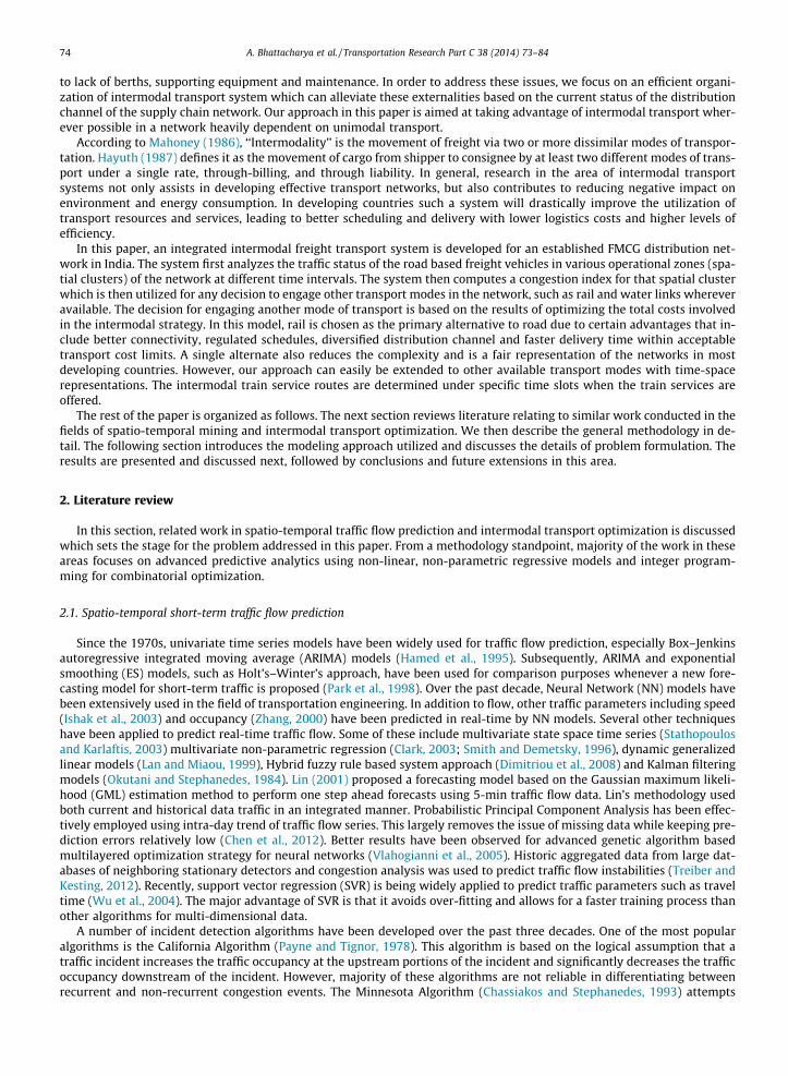
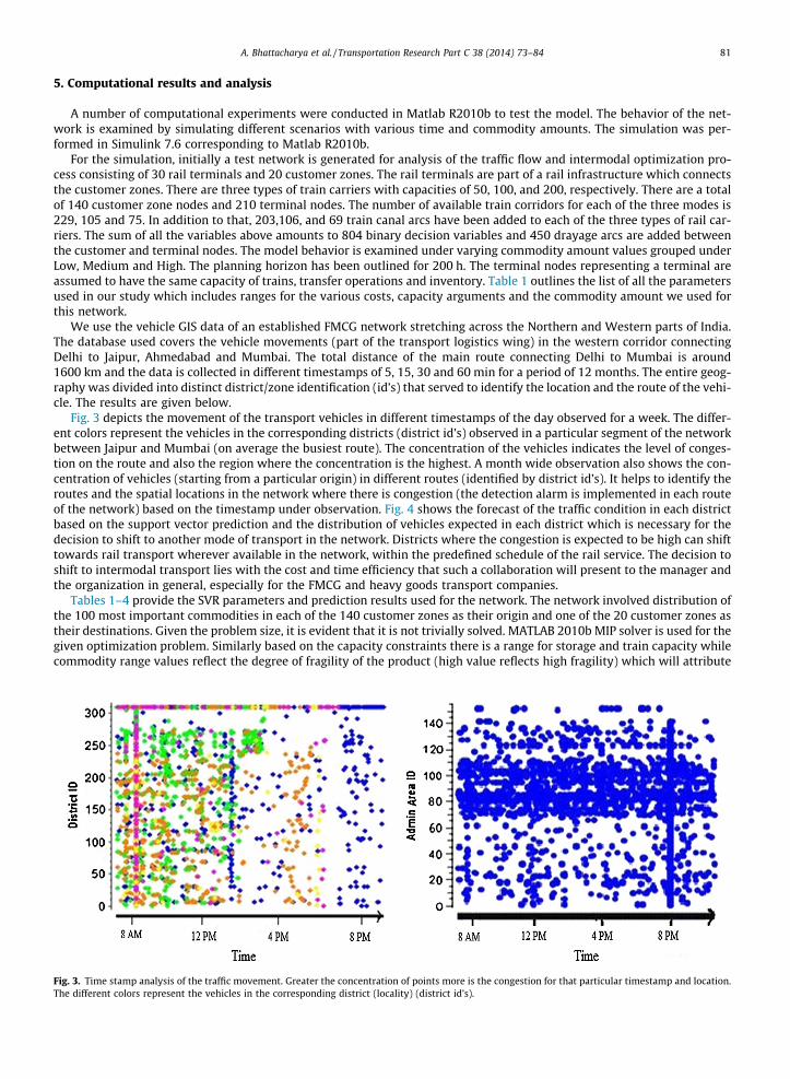
Fig. 3 depicts the movement of the transport vehicles in different timestamps of the day observed for a week. The differ-ent colors represent the vehicles in the corresponding districts (district id’s) observed in a particular segment of the networkbetween Jaipur and Mumbai (on average the busiest route). The concentration of the vehicles indicates the level of conges-tion on the route and also the region where the concentration is the highest. A month wide observation also shows the con-centration of vehicles (starting from a particular origin) in different routes (identified by district id’s). It helps to identify theroutes and the spatial locations in the network where there is congestion (the detection alarm is implemented in each routeof the network) based on the timestamp under observation. Fig. 4 shows the forecast of the traffic condition in each districtbased on the support vector prediction and the distribution of vehicles expected in each district which is necessary for thedecision to shift to another mode of transport in the network. Districts where the congestion is expected to be high can shifttowards rail transport wherever available in the network, within the predefined schedule of the rail service. The decision toshift to intermodal transport lies with the cost and time efficiency that such a collaboration will present to the manager andthe organization in general, especially for the FMCG and heavy goods transport companies.

Tables 1–4 provide the SVR parameters and prediction results used for the network. The network involved distribution ofthe 100 most important commodities in each of the 140 customer zones as their origin and one of the 20 customer zones astheir destinations. Given the problem size, it is evident that it is not trivially solved. MATLAB 2010b MIP solver is used for thegiven optimization problem. Similarly based on the capacity constraints there is a range for storage and train capacity whilecommodity range values reflect the degree of fragility of the product (high value reflects high fragility) which will attribute

Fig. 3. Time stamp analysis of the traffic movement. Greater the concentration of points more is the congestion for that particular timestamp and location.The different colors represent the vehicles in the corresponding district (locality) (district id’s).

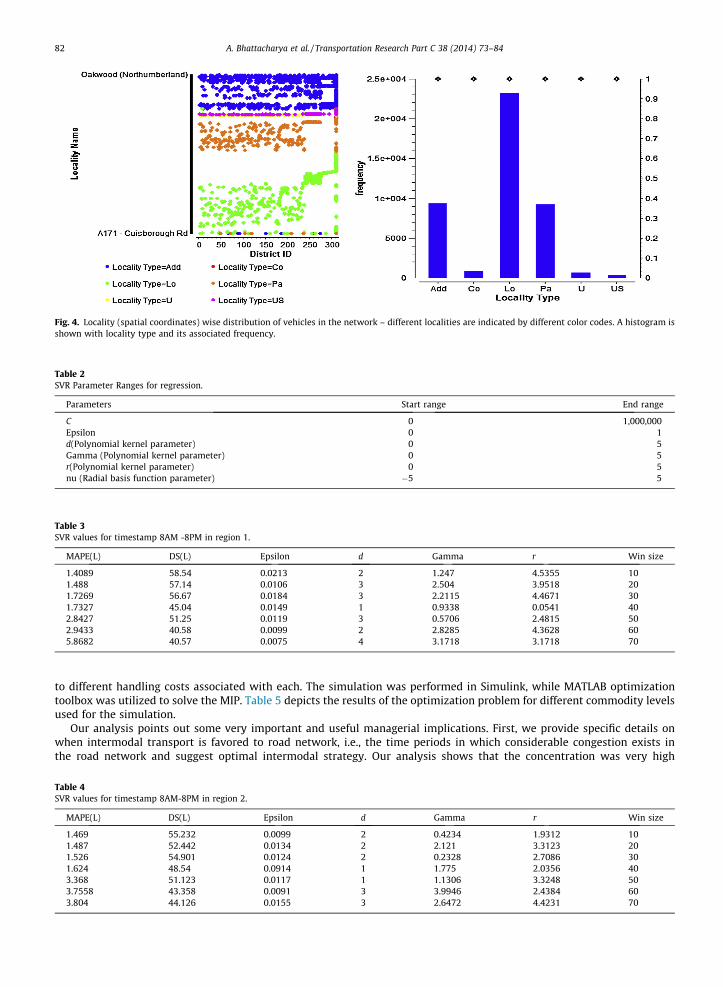
Fig. 4. Locality (spatial coordinates) wise distribution of vehicles in the network – different localities are indicated by different color codes. A histogram isshown with locality type and its associated frequency.

Table 2SVR Parameter Ranges for regression.

Parameters Start range End range

C 0 1,000,000Epsilon 0 1d(Polynomial kernel parameter) 0 5Gamma (Polynomial kernel parameter) 0 5r(Polynomial kernel parameter) 0 5nu (Radial basis function parameter) �5 5

Table 3SVR values for timestamp 8AM -8PM in region 1.

MAPE(L) DS(L) Epsilon d Gamma r Win size

1.4089 58.54 0.0213 2 1.247 4.5355 101.488 57.14 0.0106 3 2.504 3.9518 201.7269 56.67 0.0184 3 2.2115 4.4671 301.7327 45.04 0.0149 1 0.9338 0.0541 402.8427 51.25 0.0119 3 0.5706 2.4815 502.9433 40.58 0.0099 2 2.8285 4.3628 605.8682 40.57 0.0075 4 3.1718 3.1718 70

82 A. Bhattacharya et al. / Transportation Research Part C 38 (2014) 73–84

to different handling costs associated with each. The simulation was performed in Simulink, while MATLAB optimizationtoolbox was utilized to solve the MIP. Table 5 depicts the results of the optimization problem for different commodity levelsused for the simulation.

Our analysis points out some very important and useful managerial implications. First, we provide specific details onwhen intermodal transport is favored to road network, i.e., the time periods in which considerable congestion exists inthe road network and suggest optimal intermodal strategy. Our analysis shows that the concentration was very high

Table 4SVR values for timestamp 8AM-8PM in region 2.

MAPE(L) DS(L) Epsilon d Gamma r Win size

1.469 55.232 0.0099 2 0.4234 1.9312 101.487 52.442 0.0134 2 2.121 3.3123 201.526 54.901 0.0124 2 0.2328 2.7086 301.624 48.54 0.0914 1 1.775 2.0356 403.368 51.123 0.0117 1 1.1306 3.3248 503.7558 43.358 0.0091 3 3.9946 2.4384 603.804 44.126 0.0155 3 2.6472 4.4231 70

Table 5Computational scenario results.

Flow Low Medium High

Number of feasible solutions 15 10 4Best feasible solution value ($) 1,068,860 1,444,330 1,746,030Lower bound at time limit 617,764 905,356 1,136,908Lower bound/best feasible solution gap 42.20% 37.31% 34.84.5%LP solution time (sec.) 250 275 326LP solution 978,007 1,281,120 1,438,729LP/Best feasible solution gap (%) 8.5 11.3 17.6

Table 6Time/cost tradeoff results of the network.

Time value Low Medium High

Operating costs ($) 2,856.030 3,245.810 3,951.580Number of train services utilized 22 26 35Train services available 51 43 67Service capacity index 234 322 466Total transit time 217.500 179.832 173.700Transit time decrease (low time ? med. time; med. time ? high time) (%) 17.32 3.41 3.41Service utilization (%) 65.27 55.34 41.19Total handling operations 3560 3122 3345

A. Bhattacharya et al. / Transportation Research Part C 38 (2014) 73–84 83

between 8AM to 12PM in most of the district id’s. The congestion detection level was high in this period for all range of time-stamps considered, and the support vector forecast also supports the trend for high congestion in the intervals considered.This necessitates the use of intermodal transport in this period while it has to satisfy the overall cost and time limits.

The computation results for the intermodal optimization show that it is difficult problem to solve. Within a simulationtime limit of 5 h, we identified feasible solutions for the different scenarios within acceptable limits from the best feasiblesolutions. The gap between the corresponding linear program (LP) and best solution is 8.5%, 11.3% and 17.6% respectively fordifferent cargo flow scenarios. The overall analysis shows that the operational costs increase with the number of commod-ities, the fragility quotient of the commodities involved, and with transshipment time.

Table 6 provides the results for the various factors of our optimization study. The higher the value of time, higher is theoperational cost and the number of feasible solutions decrease. This implies that when the time value increases, the systemtries to incorporate more services in a specific time interval for faster transit times, which results in higher operational andhandling costs, which is the classic tradeoff between time and cost. Higher time values ensures shorter transit times andmore capacity handling. More train canals are thus chosen when there is higher capacity handling, leading to faster servicesat higher prices which might be acceptable depending on the company’s strategy and urgency of transporting the goods. Theanalysis further shows that high capacity train canals are chosen for high to medium time values, thus effectively increasingavailable capacity and leading to corresponding decrease in service utilization. Higher number of services implies fewertransfers and shorter inventory holding time during transshipment. Thus, a transport manager of any logistics departmentcan effectively decide on using the intermodal transport strategy based on the congestion analysis and cost-time tradeoffinvolving an alternate mode (in our case railways).

The model developed here may very well be adapted to other networks with shorter route distances. Shorter route dis-tances would mean lesser number of district-id’s, where traffic congestion would need to be monitored. It is prudent to as-sume that for short distances the inter-modal transport system should be invoked only if traffic congestion levels areunbearable. The reason being that the dramatic increase in cost that would arise if an inter-modal network was used for thisscenario. However, this can easily be considered in the model development by defining the Det_Lev_limit (Section 4.1) appro-priately, in accordance with the given conditions.

6. Conclusions and extensions

In this paper a basic architecture for traffic flow analysis and decision support for intermodal transport mechanism is pre-sented. Mathematical models for predicting future traffic congestion in roads and intermodal transport cost optimization isformulated and analyzed. Insightful managerial implications are presented based on the simulation results of the intermodaltransport strategy. The model application received favorable support from the FMCG company executives. The model isimplemented in a generic fashion which can be customized according to the area of application and the need of the organi-zation using it. Future research should investigate the use of multivariate time series models that incorporate spatial andtemporal correlations among adjacent Vehicle Detection Stations (VDS) to improve prediction accuracy, especially whenmulti-step look-ahead forecasts are desired. In addition, future work may evaluate the performance of SVR for various

84 A. Bhattacharya et al. / Transportation Research Part C 38 (2014) 73–84

look-back intervals, forecasting horizons, and data resolutions. For the intermodal strategy, heuristic methods can prove tobe a quick and efficient way of finding feasible solutions. We believe the next step is to research how to handle the new set ofconstraints for network design models before proceeding to applying such models to real instances.

References

Caprara, A., Malaguti, E., Toth, P., 2011. A freight service design problem for a railway corridor. Transportation Science 45 (2), 147–162.Chassiakos, A.P., Stephanedes, Y.J., 1993. Smoothing algorithms for incident detection. Transportation Research Record 1394, 8–16.Chen, C., Wang, Y., Li, L., Hu, J., Zhang, Z., 2012. The retrieval of intra-day trend and its influence on traffic prediction. Transportation Research Part C 22, 103–

118.Clark, S., 2003. Traffic prediction using multivariate nonparametric regression. Journal of Transportation Engineering 129 (2), 161–168.Dimitriou, L., Tsekeris, T., Stathopoulos, A., 2008. Adaptive hybrid fuzzy rule-based system approach for modeling and predicting urban traffic flow.

Transportation Research Part C 16, 554–573.Gorman, M.F., 1998. An application of genetic and Tabu searches to the freight railroad operating plan problem. Annals of Operations Research 78, 51–69.Hamed, M.M., Al-Masaeid, H.R., Said, Z.M., 1995. Short-term prediction of traffic volume in urban arterials. Journal of Transportation Engineering 121 (3),

249–254.Hayuth, Y., 1987. Intermodality: Concept and Practice, Structural Changes in the Ocean Freight Transport Industry. Lloyd’s University Press, London.Ishak, S., Kotha, P., Alecsandru, C., 2003. Optimization of dynamic neural network performance for short-term traffic prediction. Transportation Research

Record 1836, 45–56.Lan, C.J., Miaou, S.P., 1999. Real-time prediction of traffic flows using dynamic generalized linear models. Transportation Research Record 1678, 168–178.Lin, W.H., 2001. A Gaussian maximum likelihood formulation for short-term forecasting of traffic flow. In: Proceedings of the IEEE Intelligent Transportation

Systems Conference, pp. 150–155.Mahoney, J.H., 1986. Intermodal freight transportation. Transportation Quarterly 40 (1), 85–88.Ma, J., James, T., Simon, P., 2003. Accurate online support vector regression. Neural Computation 15, 2683–2703.Newman, A.M., Yano, C.A., 2000. Scheduling direct and indirect trains and containers in an intermodal setting. Transportation Science 34 (3), 256–270.Okutani, I., Stephanedes, Y., 1984. Dynamic prediction of traffic volume through Kalman filtering theory. Transportation Research Part B 18 (1), 1–11.Park, B., Messer, C.J., Urbanik, T., 1998. Short-term traffic volume forecasting using radial basis function neural network. Transportation Research Record

1651, 39–47.Payne, H.J., Tignor, S.C., 1978. Freeway incident detection algorithms based on decision tree with states. Transportation Research Record 682, 378–382.Smith, B.L., Demetsky, M.J., 1996. Multiple-interval freeway traffic flow forecasting. Transportation Research Record 1554, 136–141.Southworth, F., Peterson, B., 2000. Intermodal and international freight network modeling. Transportation Research Part C 8, 147–166.Stathopoulos, A., Karlaftis, M.G., 2003. A multivariate state space approach for urban traffic flow modeling and prediction. Transportation Research Part C

11, 121–135.Treiber, M., Kesting, A., 2012. Validation of traffic flow models with respect to the spatio temporal evolution of congested traffic patterns. Transportation

Research Part C 21, 31–41.Vapnik, V.N., 1995. The nature of statistical learning theory. Springer, New York.Vlahogianni, E., Karlaftis, G., Golias, J., 2005. Optimized and meta-optimized neural networks for short-term traffic flow prediction: a genetic approach.

Transportation Research Part C 13, 211–234.Wong, R.C.W., Yuen, T.W.Y., Fung, K.W., Leung, J.M.Y., 2008. Optimizing timetable synchronization for rail mass transit. Transportation Science 42 (1), 57–

69.Wu, C.H., Ho, J.M., Lee, D.T., 2004. Travel-time prediction with support vector regression. IEEE Transactions on Intelligent Transportation Systems 5 (4), 276–

281.Yamada, T., Russ, B.F., Castro, J., Taniguchi, E., 2009. Designing multimodal freight transport networks: a heuristic approach and applications. Transportation

Science 43 (2), 129–143.Yano, C.A., Newman, A.M., 2001. Scheduling trains and containers with due dates and dynamic arrivals. Transportation Science 35 (2), 181–191.Zeng, D., Xu, J., Gu, J., Liu, L., 2008. Short term traffic flow prediction based on online learning. SVR Workshop on Power Electronics and Intelligent

Transportation System (PEITS ‘08).Zhang, H.M., 2000. Recursive prediction of traffic conditions with neural network models. Journal of Transportation Engineering 126 (6), 472–481.