an integrated load-planning problem with intermediate consolidated truckload assignments
TRANSCRIPT

IIE Transactions (2010) 42, 490–513Copyright C© “IIE”ISSN: 0740-817X print / 1545-8830 onlineDOI: 10.1080/07408170903468571
An integrated load-planning problem with intermediateconsolidated truckload assignments
HALIT USTER1,∗ and HOMARJUN AGRAHARI2
1Department of Industrial and Systems Engineering, Texas A&M University, College Station, TX 77843-3131, USAE-mail: [email protected] Design and Performance, BNSF Railway, Fort Worth, TX 76131-1322, USA
Received August 2008 and accepted October 2009
This article considers an integrated load-planning problem where decisions on how commodities with unique origin–destination nodesare routed over a given transportation network, along with decisions on their explicit consolidation and assignment to capacitatedtruckloads, are addressed. In a logistical context, a commodity may refer to a shipper’s load handled by a freight forwarder whoworks as an intermediary between the shippers and carriers. A compact formulation that addresses the load consolidations frommany shippers into truckloads and the associated transportation decisions explicitly is first provided. Then, to develop efficientsolution algorithms, four compound neighborhood functions and a branching scheme are suggested. Each compound neighborhoodfunction has two main components, level change and content change, with the latter based on various schemes of combiningsimple neighborhood functions. The compound neighborhood functions and branching strategies enable the solution space to beefficiently searched. Two heuristic algorithms (one with deterministic and the other with probabilistic features) and a tabu searchalgorithm are also developed. The two components of compound neighborhood functions provide the means to efficiently incorporateintensification and diversification characteristics into these algorithms. Extensive computational results illustrating and comparingthe relative efficiency and effectiveness of the algorithms and the compound neighborhood functions are reported. The alternativecompounding schemes and the search strategies provided in this study are potentially useful in other problem domains as well.
Keywords: Transportation, load planning, heuristic algorithms, compound neighborhoods
1. Introduction
Multi-commodity flows appear frequently in various logis-tical applications where there is a significant flow of en-tities such as raw materials, spare parts, work-in-process,finished products, parcels/packages, and passengers. Thecommon characteristic of these applications is the exis-tence of uniquely defined flow requirements (commodities)between the origin–destination physical node pairs on thenetwork. Typical applications arise in the context of logis-tics, including regional and global supply-chain logistics,third-party logistics, and freight forwarding. For example,freight forwarders work as intermediaries with many ship-pers and transportation companies and handle the freightof shippers via efficiently planning their transportation us-ing the services provided by carriers. In some cases, largecorporations that operate many plants and spare part fa-cilities act as their own freight forwarders or transporta-tion planners to better plan for shipment of componentsamong their facilities. The effectiveness in such distribu-
∗Corresponding author
tion systems relies heavily on the transportation economies-of-scale achieved via load consolidations. The main opera-tional characteristic that defines our problem setting is thatthe flows originating in the origin nodes are first temporar-ily collected at “consolidation centers.” Then, the consol-idated loads are transferred to “deconsolidation centers”over “line-haul, transfer” linkages, and finally the flows aredistributed from deconsolidation centers to their final des-tinations. We also allow direct shipments between originand destination nodes since this is preferred when the ori-gin and destination nodes of a commodity are relativelyclose or when a commodity’s flow is large, and, thus, con-solidation does not make economic sense.
Considering a general physical network (e.g., a roadnetwork) with a node set N , an “auxiliary” networkG = (V, A) under the consolidation, line-haul, and de-consolidation activities can be constructed as follows. Wefirst define the following sets: P = {p1, . . . , pN} is theset of required commodity flows; F = { fp1, . . . , fpN} andT = {tp1, . . . , tpN} represent the sets of nodes representingcommodity origins and destinations, respectively. The setsJ and K are the physical nodes (not necessarily disjoint)where the consolidation and deconsolidation activities take
0740-817X C© 2010 “IIE”

An integrated load-planning problem 491
place, respectively. We next introduce arc sets AFJ , AJK ,and AKT , which are between F and J , J and K, andK and T , respectively. The length of an arc correspondsto the shortest or a specified path length represented bythis arc on the physical network. Then, we define three di-rected bipartite graphs which we concatenate with over-lapping common nodes to form the auxiliary network.The first such graph is GC(F ∪ J , AFJ ) for consolida-tion; the second is GL(J ∪ K, AJK ) for line-haul; and thethird is GD(K ∪ T , AKT ) for deconsolidation. Thus, wehave V = F ∪ J ∪ K ∪ T and A = AFJ ∪ AJK ∪ AKT . Fi-nally, we add to A the set of arcs ( fpi , tpi ), ∀ pi ∈ P , whichrepresent possible direct shipments.
Since the collection process from origin nodes to consoli-dation centers and the distribution process from deconsoli-dation centers to final destinations involve smaller loads, weconsider the case where the shipments at these stages use theLTL (Less-Than-Truckload) mode of transportation, andthus the costs are based on the load amount and the dis-tance. Typically, a constant dollar value per pound per mileof shipment is used to represent LTL-type costs. Note thatthis also applies to direct shipments. On the other hand,since consolidated larger loads (truckloads) are transferredbetween consolidation and deconsolidation centers, weconsider the case where the shipments at this intermedi-ate stage utilize the TL (TruckLoad) mode, thus incurringper mile full TL costs for this stage. In this case, a constantper mile dollar value for dispatching a truck is used to cal-culate the total cost of a shipment between two centers. Weassume that high-volume commodities that justify a TLshipment are also shipped directly. For the case in whichsuch direct shipments can be identified a priori, the asso-ciated direct TL shipment costs are considered to be sunkcosts; thus, we do not include these commodities in ourmodel. Alternatively, our model can easily accommodatedirect shipment decisions for high-volume commodities.
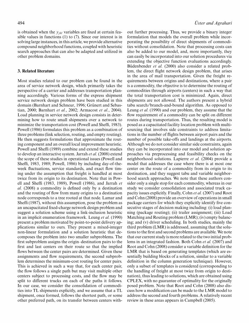
For illustration purposes, consider a general physical net-work with N = {1, . . . , 11} of which nodes 5, 6, 8, and 10are centers as depicted in Fig. 1. That is, both sets J and K
9
5
10
1
4
8
2
11
3
7
6
fp1
tp1
fp2
tp2
fp3
tp3
fp4
tp4
fp5
tp5
fp6
tp6
fp7
tp7
fp8
tp8
Fig. 1. Required commodity flows on a physical network.
8
5
10
6
8
5
10
6
F J K Tfp1 tp1
fp2 tp2
fp3 tp3
fp4 tp4
fp5 tp5
fp6 tp6
fp7 tp7
fp8 tp8
Fig. 2. An example routing in the auxiliary network.
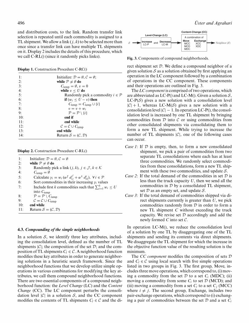
are given by the node set {5, 6, 8, 10} in this case. The originsand destinations of eight commodities are also shown onthe physical network. An example flow of commodities onthe corresponding auxiliary graph is shown in Fig. 2, whichimplies that commodities p1, p2, p6, and p7 are shipped viaLTL mode to the center at node 5 for consolidation intotwo TL shipments. One TL includes p1 and p2 and is trans-ferred over a line-haul link to the center at node 6 for de-consolidation; from there, the individual commodities areshipped to their final destinations. The other TL consol-idates p6 and p7 and transfers them to center at node 8for deconsolidation. Similarly, commodities p3, p4, and p5are consolidated into a TL shipment and transferred fromthe consolidation center at node 6 to the deconsolidationcenter at node 10. Note that the total commodity flow as-signed for each line-haul is assumed to be less than the TLcapacity. In this example, node 6 serves as both a consol-idation and a deconsolidation center. Finally, commodityp8 is sent via direct shipment.
Under these operational and configurational characteris-tics, we address, in an integrated fashion, the load-planningproblem, which corresponds to finding the routing for aload in the transportation network as well as the explicitconsolidation and assignment of loads to capacitated TLson the line-haul links. Thus, our purpose is to determinethe line-haul links between the regional centers (consoli-dation and deconsolidation centers at known locations),the routing and consolidation of commodities (includingdirect shipments), the explicit assignment of these consol-idated loads to trucks, and the assignment of truckloadsto the line-haul links. In doing so, we aim to minimize thetotal associated transportation cost, which has four com-ponents: the costs of (i) collection; (ii) distribution; (iii)line-haul transfer from consolidation to deconsolidationcenters; and (iv) direct shipments.
In this article, first we provide a compact formulationfor this load-planning problem by taking into accountthe above-described common underlying practice in the

492 Uster and Agrahari
operation of these specially structured systems. Specifically,our model addresses how the consolidation is achieved andthe associated costs as well as the operational simplicityassociated with handling freight via only one pair of con-solidation/deconsolidation centers. Typically, in logisticsnetworks, an excessive number of handlings (processing)of freight is highly undesirable due to the prohibitivecost implications. Furthermore, with our formulation, weefficiently integrate problems involving the assignment ofloads to TLs and the assignment of these TLs to the line-haul links. Second, we present four types of neighborhoodfunctions, where each is obtained via compounding moveand exchange-based simple neighborhood functions thatare aligned with our solution representation. In general,solution representations that facilitate the consideration ofa rich set of simple neighborhoods are good candidates forgenerating compound neighborhoods. Third, aligned withour solution representation and compounding of neigh-borhoods, we introduce a branching scheme to facilitate anefficient search of the solution space. We incorporate thisscheme into two solution improvement algorithms, onecreating search trajectories in a deterministic fashion andthe other in a probabilistic fashion. In the latter, we borrowfrom the simulated annealing acceptance probabilityapproach; however, we apply it to a set of (neighboring)solutions represented by a simple neighborhood functioninstead of the individual solution that would be obtainedby the neighborhood function in a conventional appli-cation. In addition, we devise a tabu search procedureincorporating our neighborhood functions and branchingscheme. Lastly, we present an extensive set of computa-tional studies to analyze the effectiveness of the alternativealgorithmic frameworks and neighborhood functions,which correspond to a total of 12 approaches obtainedvia three algorithmic frameworks and four compoundneighborhood structures. Whenever possible, we employCPLEX 11.0 to obtain benchmark results, and, at othertimes, we utilize the best solution we obtain as the baseand measure the relative goodness of the approachesaccordingly.
The remainder of this article is organized as follows.Next, in Section 2, we develop a binary integer programformulation for our problem. This is followed by a review ofthe related literature in Section 3. In Section 4, we describethe basic ingredients of our heuristic solution approachesin detail, including the compound neighborhood functions.In Section 5, we present three algorithmic frameworks in-cluding two solution improvement algorithms (one withdeterministic and one with probabilistic search features)and tabu search, where, in each approach, we employ asolution neighborhood exploration strategy that relies onbranching based on solution representation characteristics.In Section 6, we present the results of our computationaltests regarding the performance of the approaches and inSection 7 we provide a summary of our conclusions andfuture research directions.
2. The model formulation
In order to develop a mathematical formulation of our dis-tribution network design problem by utilizing the auxiliarygraph, we define the following additional notation.Parameters
wi = the amount of flow for commodity pi ;U = capacity per full TL for long-haul transfers;β = full TL transportation cost per mile betweenJ and
K;αf = LTL transportation cost per unit per mile between
F and J ;αt = LTL transportation cost per unit per mile between
K and T ;α = LTL transportation cost per unit per mile between
F and T ;d f
i j = distance between fpi and consolidation center j ;dt
ki = distance between deconsolidation center k and tpi ;d jk = distance between centers j and k;di = direct shipment distance for commodity pi ;L = set of line-haul trucks (TL shipments), l =
1, . . . , |L|.Decision variables⎧⎨
⎩zi jkl = 1 if commodity pi is assigned to TL l ∈ L
installed on line-haul link ( j, k),0 otherwise.⎧⎨
⎩yjkl = 1 if TL shipment l is assigned to the line-haul
link ( j, k),0 otherwise.⎧⎨
⎩si = 1 if commodity pi is shipped directly from
its origin to its destination,
0 otherwise.
min∑i∈P
∑j∈J
∑k∈K
∑l∈L
wi(αf df
i j + αt dtki
)zi jkl
+∑j∈J
∑k∈K
∑l∈L
β d jk yjkl +∑i∈P
α wi di si , (1)
subject to∑j∈J
∑k∈K
∑l∈L
zi jkl + si = 1 ∀ i ∈ P, (2)
∑i∈P
∑j∈J
∑k∈K
wi zi jkl ≤ U∑j∈J
∑k∈K
yjkl ∀ l ∈ L, (3)
zi jkl ≤ yjkl ∀ i ∈ P, j ∈ J , k ∈ K, l ∈ L, (4)∑j∈J
∑k∈K
yjkl ≤ 1 ∀ l ∈ L, (5)
∑j∈J
∑k∈K
yj,k,l+1 ≤∑j∈J
∑k∈K
yjkl , l = 1, . . . , |L| − 1, (6)
zi jkl , si , yjkl ∈ {0, 1} ∀ i ∈ P, j ∈ J , k ∈ K, l ∈ L. (7)

An integrated load-planning problem 493
In the objective function (1), the first term represents thetotal transportation cost for collection and distributionoperations in GC(F ∪ J , AFJ ) and GD(K ∪ T , AKT ), re-spectively; the second term represents the total transporta-tion cost for linehaul transfers using a TL shipment inGL(J ∪ K, AJK ); and the third term represents the totaltransportation cost for commodities shipped directly fromorigin to destination. Constraint set (2) states that eachcommodity is either included in a TL shipment or shippeddirectly. Constraint set (3) ensures that the total weight ofthe commodities assigned to a TL shipment does not ex-ceed the capacity of a truck. We estimate the maximumsize of the set L as �∑i∈P wi/(0.75 U)�, which is obtainedby assuming that, on average, 75% full TLs justify con-solidated shipments. While this estimate is conservative, inour numerical studies we observe that set L is never ex-hausted. Constraint set (4) ensures that a commodity canbe assigned to a TL shipment on a particular line-haultransfer link only if this link has that TL installed on it.This constraint, although redundant since it is implied bythe previous constraint, helps greatly in obtaining betterlower bounds when linear programming relaxation is usedin a branch-and-cut framework. Constraint set (5) ensuresthat each potential TL is assigned to, at most, one line-haul transfer link. Constraint set (6) helps to reduce thesymmetry in allocating line-haul trucks to transfer links.Specifically, they reduce the solution space by utilizing theTLs in order, e.g., everything else being same, having TLl = 5 without having TL l = 4 versus having TL l = 4 with-out having TL l = 5 in a solution are essentially equivalent.Constraint set (7) imposes standard binary restrictions onthe decision variables.
An important characteristic of our model is that, with theintroduction of dummy consolidation centers, commoditiesoriginating at the same physical node can be consolidatedat their source. Specifically, each node in N − J in whichat least a commodity originates can be designated as adummy consolidation center and included in the set J .For a dummy center j , the distance d f
i j associated with acommodity i that does not originate at j is set to infinity.A similar modification to the input data can be done byintroducing dummy deconsolidation centers from the setN − K so that the commodities destined to the same phys-ical node can be deconsolidated at their destination. Notethat this modification also facilitates the direct shipment ofhigh-volume commodities under TL costs. Another impor-tant characteristic of the model is its simple, yet effective,consideration of transportation economies-of-scale realizedthrough TL consolidations using capacitated trucks. In ad-dition, any fixed costs associated with TL shipments canalso be easily incorporated into the second term of theobjective function.
Furthermore, we observe that our problem is also relatedto the Single-Source Capacitated Facility Location Prob-lem (SSCFLP), which is a special case of our problem. InSSCFLP, given the potential facility locations with known
capacities, the objective is to minimize the total cost oflocation and transportation while satisfying customer de-mands in such a way that each customer is assigned to asingle facility. A solution to our problem consists in somecommodities being assigned to TL shipments on line-haultransfer links, with the remaining commodities, if present,being shipped via direct shipments. One can view a po-tential TL shipment on a transfer link as a capacitatedfacility and the commodities as the customers. In order tomodel the direct shipments, we can create a pair of dummyconsolidation–deconsolidation centers for each commod-ity and define the cost of assigning the commodity to itsdummy center pair as equivalent to the cost of a directshipment with zero collection and distribution costs (costsassociated with other commodities and the dummy link aresimply taken as infinity). Then, clearly, our problem gener-alizes SSCFLP. However, from the perspective of a typicalSSCFLP setting, our problem is too large for state-of-the-art methods to solve. For example, let M be the number ofcenters and L be the number of potential TL shipments. Re-call that N is the number of commodities. Then, an equiv-alent SSCFLP will have L M2 + N potential facilities andN customers. In an instance with 500 commodities on anetwork with M = 6 and L = 20, the equivalent SSCFLPwill have 20 × 36 + 500 = 1220 potential locations and 500customers. Typically, SSCFLPs that are much smaller insize are considered difficult in the literature (Cortinhal andCaptivo, 2003). Furthermore, an equivalent SSCFLP ver-sion of our problem has a significantly higher number ofpotential locations than the number of customers, whichis quite the opposite of a typical facility location problemwhere the number of potential locations is very small whencompared with the number of customers. Therefore, even asmall instance of our problem is actually prohibitively largefor state-of-the-art methods to solve efficiently.
We use the formulations (1) to (7) to find optimal solu-tions to small problem instances by using CPLEX, whichemploys branch-and-cut methodology with several cut op-tions, preprocessing, upper bound heuristics, and dynamicbranching strategies. For these instances, the formulationcan be solved to optimality efficiently; however, the com-putational time to close the optimality gaps and memoryrequirements become quite prohibitive for larger instances.Even for the instances with 60 commodities, this approachbecomes impractical from operational perspective—therun times are of the order of a few hours and the gapscan be as high as 15%, as reported in Section 6.2. Note thatthe instances that arise in real freight forwarding applica-tions may have several hundred commodities; i.e., pairs oforigin–destination locations. The difficulty of the problemis not surprising because several special cases of this prob-lem are well-known NP-hard problems; e.g., the previouslydescribed SSCFLP and other fixed-charge discrete locationproblems (capacitated or uncapacitated). Furthermore, thegeneralized assignment problem, which is a notoriously dif-ficult NP-hard problem, is a special case of our problem; it
494 Uster and Agrahari
is obtained when the yjkl variables are fixed at certain fea-sible values in functions (1) to (7). Since our interest is insolving large instances, in this article, we provide alternativecompound neighborhood functions, coupled with heuristicsearch approaches that can also be adapted and utilized inother problem domains.
3. Related literature
Most studies related to our problem can be found in thearea of service network design, which primarily takes theperspective of a carrier and addresses transportation plan-ning accordingly. Various forms of the express shipmentservice network design problem have been studied in thisdomain (Barnhart and Schneur, 1996; Grunert and Sebas-tian, 2000; Barnhart et al., 2002; Armacost et al., 2004).Load planning in service network design consists in deter-mining how to route small shipments over a network tominimize the transportation cost (Powell and Sheffi, 1983).Powell (1986) formulates this problem as a combination ofthree problems (link selection, routing, and empty routing).He then suggests formulations that approximate the rout-ing component and an overall local improvement heuristic.Powell and Sheffi (1989) combine and extend these studiesto develop an interactive system. Jarrah et al. (2008) extendthe scope of these studies in operational issues (Powell andSheffi, 1983, 1989; Powell, 1986) by including day-of-the-week fluctuations, service standards, and exact flow tim-ing under the assumption that freight is handled at mosttwice from its origin to its destination. Note that in Pow-ell and Sheffi (1983, 1989), Powell (1986), and Jarrah etal. (2008) a commodity is defined only by a destinationand the routing of flow from many origins to a destinationnode corresponds to a tree rooted at that node. Lamar andSheffi (1987), without this assumption, pose the problem asan uncapacitated fixed-charge network design problem andsuggest a solution scheme using a link-inclusion heuristicin an implicit enumeration framework. Leung et al. (1990)present a problem motivated by point-to-point delivery ap-plications similar to ours. They present a mixed-integernon-linear formulation and a solution heuristic that de-composes the problem into two smaller subproblems. Thefirst subproblem assigns the origin–destination pairs to thefirst and last centers on their route so that the impliedflows between the center pairs are determined. Given theseassignments and flow requirements, the second subprob-lem determines the minimum-cost routing for center pairs.This is achieved in such a way that, for each center pair,the flow follows a single path but may visit multiple othercenters subject to processing costs, and the flow may besplit to different trucks on each of the paths it follows.In our case, we consider the consolidation of commodi-ties into TL shipments explicitly, and we assume that a TLshipment, once formed, follows the shortest path, or someother preferred path, on its transfer between centers with-
out further processing. Thus, we provide a binary integerformulation that models the overall problem while incor-porating the possibility of direct shipments of commodi-ties without consolidation. Note that processing costs canalso be added to our model, and, more importantly, theycan easily be incorporated into our solution procedures viaextending the objective function evaluations accordingly.Budenbender et al. (2000) also consider a related prob-lem, the direct flight network design problem, that arisesin the area of mail transportation. Given the freight re-quirements between origins and destinations, where a pairis a commodity, the objective is to determine the routing ofcommodities through airports (centers) in such a way thatthe total transportation cost is minimized. Again, directshipments are not allowed. The authors present a hybridtabu search/branch-and-bound algorithm. As opposed toLeung et al. (1990) and our problem, they assume that theflow requirement of a commodity can be split on differentroutes during transportation. Thus, the resulting model isposed as a capacitated facility location problem with multi-sourcing that involves side constraints to address limita-tions in the number of flights between airport pairs and thenumber of possible take-offs and landings at the airports.Although we do not consider similar side constraints, againthey can be incorporated into our model and solution ap-proaches via preprocessing and feasibility checks on theneighborhood solutions. Lapierre et al. (2004) provide amodel that addresses the case where there is at most onecenter on the route of a commodity from its origin to itsdestination, and they suggest tabu and variable neighbor-hood search approaches. We note that these authors con-sider only a single stop for each commodity, whereas in ourstudy we consider consolidation and associated truck ca-pacity issues explicitly. Finally, Cohn et al. (2007) and Rootand Cohn (2008) provide an overview of operations in smallpackage carriers for which they explicitly identify five con-secutive stages of decision making including: (i) load plan-ning (package routing); (ii) trailer assignment; (iii) LoadMatching and Routing problem (LMR); (iv) empty balanc-ing; and (v) driver scheduling. In both studies, mainly thethird problem (LMR) is addressed, assuming that the solu-tions to the first and second problems are available. We notethat our current study is more related to the two initial prob-lems in an integrated fashion. Both Cohn et al. (2007) andRoot and Cohn (2008) consider a variable definition for theLMR that is based on generating templates (which are es-sentially building blocks of a solution, similar to a variabledefinition in the column generation technique). However,only a subset of templates is considered (corresponding tothe handling of freight at most twice from origin to desti-nation), thus leading to solutions, which are obtained usingCPLEX, with no guarantee of optimality for the originallyposed problem. Note that Root and Cohn (2008) also dis-cuss how a modification can be made to the LMR model toaddress the second and fourth problems. A relatively recentreview in these areas appears in Campbell (2005).

An integrated load-planning problem 495
In the context of SSCFLP, solution approaches includeLagrangian Relaxation (LR), exact methods, and heuris-tics. The LR approaches differ from each other in terms ofthe relaxed constraints, solving the associated subproblemsand obtaining feasible solutions as upper bounds. We referto Barcelo and Casanovas (1984), Pirkul (1987), Sridharan(1993), Hindi and Pienkosz (1999), and Holmberg et al.(1999) for LR approaches that relax the assignment con-straints; to Klincewicz and Luss (1986) for an LR approachthat relaxes the capacity constraint; and to Beasley (1993)and Agar and Salhi (1998) for LR approaches that relaxboth the capacity and assignment constraints. Recently,Cortinhal and Captivo (2003) suggested the use of tabusearch in LR to obtain upper bounds. However, obtainingand keeping the feasibility in upper bounds still appear tobe challenging issues. The attempts to solve the SSCFLPusing exact methods have been few, which is not surprisingsince the problem belongs to the class of NP-hard problems.Neebe and Rao (1983) model the SSCFLP as a set parti-tioning problem and develop a column-generation-basedbranch-and-bound method. Holmberg et al. (1999) de-velop a repeated matching and Lagrangian-based branch-and-bound algorithm. Diaz and Fernandez (2002) suggesta branch-and-price framework. In terms of heuristic ap-proaches, Ahuja et al. (2004) develop a very-large-scaleneighborhood (VLSN) search algorithm which is used in amulti-start framework with the initial solutions generatedby the LR approach given in Holmberg et al. (1999). Del-maire et al. (1999) suggest a reactive greedy randomizedadaptive search procedure coupled with a tabu search. Thecomputational studies in the above span relatively small-sized problems and, as is generally the case in locationproblems, consider instances in which the number of po-tential locations is significantly less than the number ofcustomers.
4. Ingredients of our heuristic algorithms
In this section, we first describe the solution representationand objective function evaluation method, which is fre-quently used during the heuristic solution process. Later,we provide two construction heuristic approaches that areemployed to generate initial feasible solutions to be usedas inputs in the heuristic solution improvement algorithms.Also, in this section, we present the details of our compoundneighborhood functions, which are important ingredientsof the three heuristic search algorithms to be describedlater.
4.1. Solution representation and objective functionevaluation
We observe that in any feasible solution to our problem, theset of commodities is partitioned into disjoint and mutuallyexclusive subsets. One of these subsets includes commodi-
ties shipped directly from their origins to their destinations.We denote this subset by D. On the other hand, each ofthe other subsets corresponds to commodities that are in-cluded in the same TL shipment l; i.e., these commoditiesare consolidated together into the same TL shipment. Torepresent each subset of commodities forming a TL ship-ment, we use the notation Cl . Also, we denote the set ofall such subsets by C. Note that, for feasibility, we ensurethat the total weight of the commodities in a TL shipmentdoes not exceed the truck capacity. Then, the pair (C,D)represents a feasible solution to our problem. Henceforth,for notational simplicity, we represent a solution (C,D) byS.
In order to calculate the goodness of a given solution S,we need to calculate the total transportation cost it implies.For each TL shipment l, we need to determine the transferlink ( j, k), where j ∈ J and k ∈ K, that the commodities inCl use. For each Cl , we simply pick the link ( j, k) that pro-vides the lowest collection–transfer–distribution cost (firsttwo terms in the objective function) via total enumerationover the |J | × |K| transfer links. On the other hand, thecost associated with the commodities in D can be calcu-lated directly, providing the value of the last term in theobjective function. Then, the objective function value as-sociated with S is the sum of the costs associated with thecommodity subsets it involves.
4.2. Construction heuristics
Based on our solution representation, the construction ofan initial feasible solution clearly consists in partitioningcommodities into (i) TL shipments and (ii) the set of com-modities shipped directly. There are a number of possibleways to obtain such partitions. Here, we describe two initialsolution construction methods that are partially greedy innature. Both methods incorporate randomness in order tosupport a multi-start framework for improvement heuris-tics. We also note that in both of these methods we generatepurely TL shipments, since determination of a commodity’sorigin–destination proximity level for direct shipment cri-terion is difficult at this stage. Later, in the improvementheuristics, the direct shipment set D is populated and mod-ified during the search procedure.
In the first method, we randomly pick commodities toform the TL shipments, one TL shipment at a time, withoutexceeding truck capacity. The procedure stops when all thecommodities are assigned. Then, the transfer link selectionfor each TL shipment and the associated cost evaluationare performed in a greedy fashion as described above. Thisprocedure, which we refer to as C-RC() (since it randomlypicks commodities), is given in Display 1.
In the second method, we randomly select transfer links,one link at a time, and assign commodities to a TL shipmentinstalled on the selected link. After selecting a transfer link( j, k), we assign commodities in a greedy fashion based ontheir proximity, as measured by the associated collection
496 Uster and Agrahari
and distribution costs, to the link. Random transfer linkselection is repeated until each commodity is assigned to aTL shipment. We allow a link ( j, k) to be selected more thanonce since a transfer link can have multiple TL shipmentson it. Display 2 includes the details of this procedure, whichwe call C-RL() (since it randomly picks links).
Display 1. Construction Procedure C-RC()
1: Initialize: D = ∅, C = ∅;2: while P = ∅ do3: Ctemp = ∅, v = 04: while v ≤ U do5: Randomly pick a commodity i ∈ P6: if (wi ≤ U − v) then7: Ctemp = Ctemp ∪ {i}8: v = v + wi9: P = P \ {i}10: end if11: end while12: C = C ∪ Ctemp13: end while14: Return S = (C,D)
Display 2. Construction Procedure C-RL()
1: Initialize: D = ∅, C = ∅2: while P = ∅ do3: Randomly pick a link ( j, k), j ∈ J , k ∈ K4: Ctemp = ∅5: Calculate γi = wi (αf d f
i j + αt dtik), ∀ i ∈ P
6: Sort commodities in their increasing γi values7: Include first k commodities such that
∑ki=1 wi ≤ U
into Ctemp8: P = P \ Ctemp9: C = C ∪ Ctemp10: end while11: Return S = (C,D)
4.3. Compounding of the simple neighborhoods
In a solution S, we identify three key attributes, includ-ing the consolidation level, defined as the number of TLshipments |C|; the composition of the set D; and the com-position of TL shipments Cl ∈ C. A neighborhood functionmodifies these key attributes in order to generate neighbor-ing solutions in a heuristic search framework. Since theneighborhood functions that we develop utilize simple op-erations in various combinations for modifying the key at-tributes, we call them compound neighborhood functions.There are two essential components of a compound neigh-borhood function: the Level Change (LC) and the ContentChange (CC). The LC component perturbs the consoli-dation level |C| in a solution S, and the CC componentmodifies the contents of TL shipments Cl ∈ C and the di-
Move MCC MCD MDC
Exchange XCC XDC
A combination of
Content-Change (CC)Level-Change (LC)
Increase LC-P
Decrease LC-M
andS Neighbor (S)
Fig. 3. Components of compound neighborhoods.
rect shipment set D. We define a compound neighbor of agiven solution S as a solution obtained by first applying anoperation in the LC component followed by a combinationof operations in the CC component. These componentsand their operations are outlined in Fig. 3.
The LC component is comprised of two operations, whichare abbreviated as LC-P() and LC-M(). Given a solution S,LC-P(S) gives a new solution with a consolidation level|C| + 1, whereas LC-M(S) gives a new solution with aconsolidation level |C| − 1. In operation LC-P(), the consol-idation level is increased by one TL shipment by bringingcommodities from D into C or using commodities fromother consolidated shipments via consolidating them toform a new TL shipment. While trying to increase thenumber of TL shipments |C|, one of the following casescan occur.
Case 1: If D is empty, then, to form a new consolidatedshipment, we pick a pair of commodities from twoseparate TL consolidations where each has at leastthree commodities. We randomly select commodi-ties from these consolidations, form a new TL ship-ment with these two commodities, and update S.
Case 2: If the total demand of the commodities in set D isless than the truck capacity U, then we send all thecommodities in D by a consolidated TL shipment,set D as an empty set, and update S.
Case 3: If the total demand of commodities shipped via di-rect shipments currently is greater than U, we pickcommodities randomly from D in order to form anew TL shipment C without exceeding the truckcapacity. We revise set D accordingly and add thenewly formed C into set C.
In operation LC-M(), we reduce the consolidation levelof a solution by one TL by disaggregating one of the TLshipments and sending its contents via direct shipments.We disaggregate the TL shipment for which the increase inthe objective function value of the resulting solution is theminimum.
The CC component modifies the composition of sets Dand Cl ∈ C using local search with five simple operationslisted in two groups in Fig. 3. The first group, Move, in-cludes three move operations, which correspond to, (i) mov-ing a commodity from the set D to a set Ci (MDC); (ii)moving a commodity from some Ci to set D (MCD); and(iii) moving a commodity from a set Ci to a set Cj (MCC)where i = j . The second group, Exchange, includes twopair-exchange operations, which correspond to (i) exchang-ing a pair of commodities between the set D and a set Ci

An integrated load-planning problem 497
(XDC); and (ii) exchanging a pair of commodities betweena set Ci and another set Cj (XCC) where i = j . These fivesimple operations can be combined in several ways to pre-scribe different CC methods that generate a feasible (withrespect to capacity constraints) neighboring solution of agiven solution provided by the LC operation. Four suchmethods that, in turn, define four neighborhood functionscan be classified under parallel (CC-PN and CC-PLSN)and serial (CC-SN and CC-SLSN) types, as will now bedescribed.
Parallel Neighborhood (CC-PN) searches the solutionspace of a given (initial) solution S using each of thefive simple operations independently to find an improvingsolution. In each operation, the search is stopped as soonas an improving solution is obtained. For example, givenan initial solution S, the MCC operation generates andevaluates the corresponding moves in S one by one andstops as soon as an improving solution, say SMCC, isfound. This is, in a sense, completing only one iterationof a local search with MCC where the first improvingneighboring solution is the output. A similar search isapplied on the same initial solution S independently(hence the name parallel) to obtain SMCD, SMDC, SXCC,and SXDC. Then, as the neighboring solution of Sby CC-PN, the best of the five solutions is picked; i.e.,argmin{Z(SMCC), Z(SMCD), Z(SMDC), Z(SXCC), Z(SXDC)}.
Parallel Local Search Neighborhood (CC-PLSN) is simi-lar to the previous one. However, we apply a complete localsearch routine (instead of terminating after the first itera-tion) using each of MCC, MCD, MDC, XCC, and XDCas the neighborhood function separately starting with agiven solution S. In an iteration of each local search, thefirst improving solution is taken. This way, we again ob-tain five separate solutions (obtained independently) froma given initial solution S, and we pick the best one as theneighboring solution of S as in CC-PN.
Serial Neighborhood (CC-SN) utilizes the five simpleneighborhoods as does the CC-PN but in a sequentialdependent manner rather than independently. In particular,the improving solution found with a simple operationprovides the initial solution for the next operation.Observe that there are several sequences of the five simpleoperations that can be employed. We differentiate twospecific sequences: one follows the LC-P() operationand the other follows the LC-M() operation. In theformer, we denote the associated CC method as CC-SN-P, and starting with a given solution, we use thesequence MDC→XDC→XCC→MCC→MCD→XCC.In the latter, we employ the sequenceMCC→XDC→MCD→MDC→XCC, and we de-note the corresponding CC method by CC-SN-M. Forexample, in this case, given an initial solution S generatedby LC-M(), first the solution SMCC is obtained by applyingthe MCC operation to S as in CC-PN. Then, the XDCoperation is applied to SMCC to obtain SMCC, and so on.The neighboring solution of S is eventually given by thesolution obtained after the final operation; i.e., SXCC.
Serial Local Search Neighborhood (CC-SLSN), analo-gous to the relationship between the parallel-type methods,it is similar to the CC-SN. In the CC-SLSN, we conduct alocal search (instead of single iteration as in CC-SN) witheach simple operation as the neighborhood function in se-quence. Similar to the CC-SN method, we have CC-SLSN-P, which follows an LC-P() operation, and CC-SLSN-M,which follows an LC-M() operation. We employ the samesequences specified above for CC-SN-P and CC-SN-M inthe CC methods CC-SLSN-P and CC-SLSN-M, respec-tively. For example, in the CC-SLSN-P, given an solutionobtained by the LC-P() operation, we first apply a localsearch using the MDC neighborhood, and we accept thefirst improving solution at each iteration and continue theiterations until no improving solution is found. The solu-tion thus obtained is then used as the initial solution for alocal search employing the XDC neighborhood and so on.The neighboring solution of S is eventually given by thesolution obtained after the final operation; i.e., SXCC forCC-SLSN-P and SXDC for CC-SLSN-M.
A few remarks regarding the above neighborhood func-tions are in order. First, the use of the LC and CC com-ponents in this fashion facilitates the incorporation of twodesired characteristics of any heuristic search procedure.The LC component promotes diversification during thesearch of the feasible solution space. On the other hand,the methods of the CC component provide the opportunityfor intensification in a solution subspace via the combineduse of simple neighborhood functions. Second, for bothof the serial-type neighborhoods, there are several possiblesequences. We apply XCC at the end of a CC sequence (CC-SN-P or CC-SN-M) since it provides the largest search ofthe solution space. This is useful since it provides a chanceto improve the solution that was subject to several pertur-bations via other operations within the same iteration. Asa consequence, starting a new iteration again with XCC isnot expected to provide improvements at that step, whichis also the case we observed in our empirical tests.
Specifically, for CC-SN-P, LC-P is the initial operationand it increases the number of commodities sent via TL bymainly combining direct shipments into TLs. MDC sup-ports this general idea by moving direct shipments (not yetcombined into TLs) into existing TLs, if possible. This pro-vides opportunity to reach to improved solutions by takingadvantage of adding individual commodities into existingTLs. Continuing the CC-SN sequence with MCD insteadof MDC negates this effort by trying to move commoditiesto direct shipment; thus, it does not facilitate a wider ex-ploration of the solution space. On the other hand, XCD,which follows MDC, promotes the search in a larger so-lution space facilitated by additions of TLs. Next, XCCand MCC provide further exploration, which is more indi-rectly facilitated by the changes made via MDC and XDC.They are followed by MCD, which attempts to identifyany commodities that may be a better fit for direct ship-ment based on the current TL configuration. Finally, ap-plying XCC is useful for the case where some commodities

498 Uster and Agrahari
are moved to direct shipment from TLs so that com-modity exchange among TLs may provide improvement.We also observed that applying XCC after MCD pro-vides better solutions by taking advantage of newly openedspace in TLs (after moves to direct shipment by MCD)for exchanges. We specifically note that the subsequenceXDC→XCC→MCC could be lined up in a different per-mutation without a lot of impact on the solution quality;however, in our empirical tests, the reported subsequenceprovided better quality results.
For CC-SN-M, LC-M is the initial operation, whicheliminates one TL shipment by assigning its load to di-rect shipments. Since applying MDC immediately after-wards negates this effort and applying MCD is not likelyto improve the solution at this step (because it moves acommodity to direct shipment from a consolidated TL),we consider the operations MCC and XDC. In our empir-ical tests, the subsequence MCC→XDC performed better;thus, we start the CC-SN-M with this subsequence. This isfollowed by the subsequence MCD→MDC in this particu-lar order since MCD is likely to create more available capac-ity in TLs, which can then be occupied by direct shipmentsmoved to consolidations via MDC. Finally, as in CC-SN-P,we apply XCC to search a large solution space for furtherimprovements. We also note that our tests against randomlygenerated sequences of operations did not produce consis-tently better performance, if any, when compared to thesequences employed.
4.4. Generic notation and branching
We define the generic notation that we use in describing theheuristic algorithms as follows. Without specific reference,the function ConstructionHeuristic() refers to obtaining aninitial solution which can be performed by applying eitherprocedure C-RC() or C-RL().
Recall that, although it is immaterial in parallel CCneighborhoods, serial CC neighborhoods depend on theLC method used. Specifically, for a CC component, wegenerically use the function CC-P() to refer to the CC-PN,CC-PLSN, CC-SN-P, or CC-SLSN-P neighborhoods. Forexample, if the CC-PN is chosen in an algorithm, thenCC-P(S) generates the neighboring solution of S with theCC-PN method as previously defined. We use the functionCC-M() to refer to the CC-PN, CC-PLSN, CC-SN-M, andCC-SLSN-M neighborhoods.
We define a branching on a node representing a currentsolution S as shown in Fig. 4. The left child of a node S,denoted by SM, is a solution obtained by LC-M() followedby CC-M(), and the right child of a node S, denoted bySP, represents a solution obtained by LC-P() followed byCC-P(). For example, if CC-PN is chosen as the CC neigh-borhood in a heuristic algorithm, in an iteration startingwith a solution S, SM is given by the neighboring solutionobtained by the CC-PN when it is applied to the solutionprovided by LC-M(S) as shown on the arc from S to SM
S
SM SM
SMM SPP
CC-M(LC-M(S)) CC-P(LC-P(S))
CC-M(LC-M(SM )) CC-P(LC-P(SP ))
Fig. 4. Branching on a solution S.
in Fig. 4. Similarly, we obtain the solutions SMM and SPPfrom SM and SP, respectively.
Notice that the solutions that can be represented as SMPor SPM are not included in the branching. The reason forthis is that in an iteration of any of the heuristic algorithms(to be described), we mainly seek the better solutions thatcan be obtained after a LC operation. Thus, we considereither increasing or decreasing the number of TLs in thecurrent (initial) solution of an iteration. The increase ordecrease can be by either one or two TLs as implied by thetwo nodes on each branch in Fig. 4.
We note that the use of multiple neighborhood functionsis also utilized in the Variable Neighborhood Search (VNS)framework (Hansen and Mladenovic, 2003). However, inVNS, neighborhoods are generally used to facilitate diversi-fication in the search procedure without particular empha-sis on any specific structure. In several studies outlined inHansen and Mladenovic (2003), the multiple neighborhoodfunctions are obtained from one base function by varyingits parameter. For example, k-moves or k-exchanges withvarying (progressively increasing to reach to farther neigh-borhoods of a current solution) k values are considered.This is also similar to the perturbation stage of iterated lo-cal search (Lourenco et al., 2003). On the other hand, aspreviously discussed, we integrate various neighborhoodfunctions (LC-P, LC-M, MCC, MCD, MDC, XCC, andXDC) in specific ways to define new compounded neigh-borhood functions, which we employ in search proceduresalong with a branching strategy as explained in the follow-ing section.
5. Heuristic approaches
In this section, we describe three improvement heuristics,including two solution improvement routines and a tabusearch procedure. Since each of the three heuristics canemploy any one of the four compound neighborhood func-tions, given by CC-PN, CC-PLSN, CC-SN, and CC-SLSN,we have a total of 12 solution procedures.
An integrated load-planning problem 499
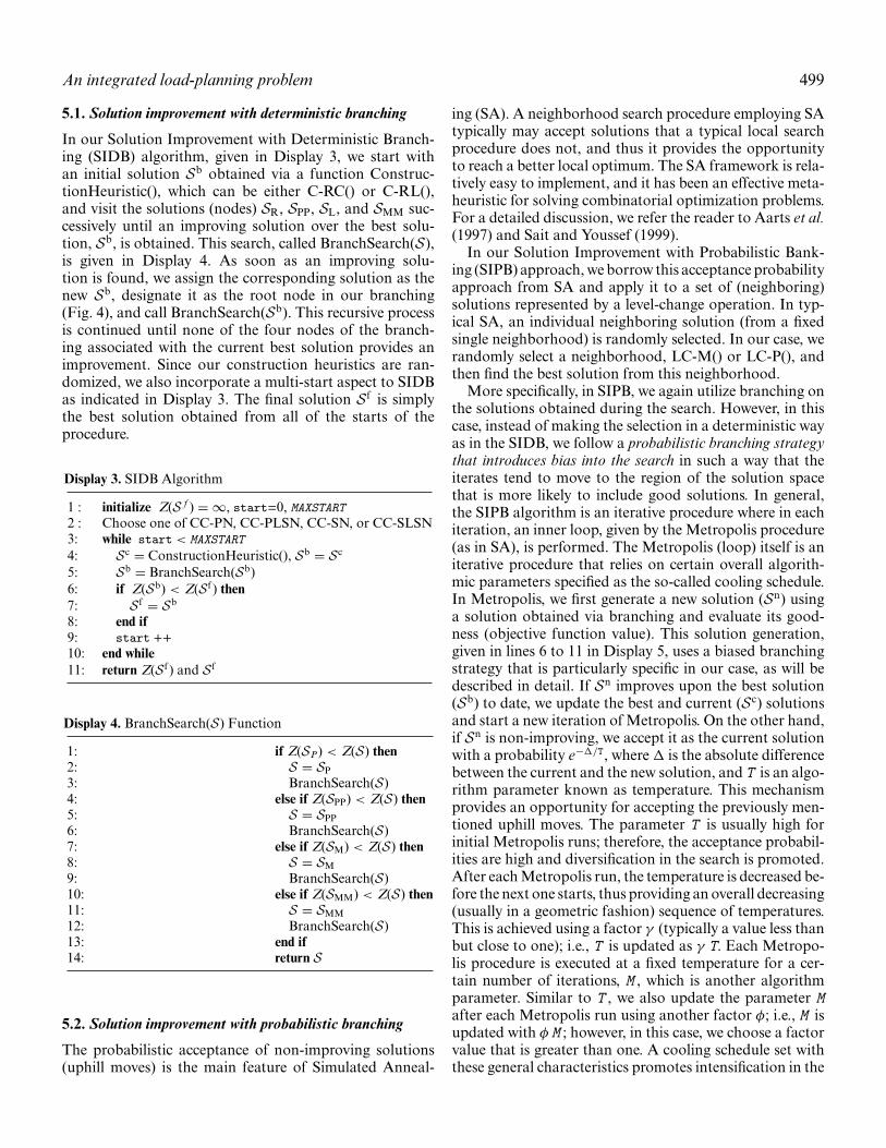
5.1. Solution improvement with deterministic branching
In our Solution Improvement with Deterministic Branch-ing (SIDB) algorithm, given in Display 3, we start withan initial solution Sb obtained via a function Construc-tionHeuristic(), which can be either C-RC() or C-RL(),and visit the solutions (nodes) SR, SPP, SL, and SMM suc-cessively until an improving solution over the best solu-tion, Sb, is obtained. This search, called BranchSearch(S),is given in Display 4. As soon as an improving solu-tion is found, we assign the corresponding solution as thenew Sb, designate it as the root node in our branching(Fig. 4), and call BranchSearch(Sb). This recursive processis continued until none of the four nodes of the branch-ing associated with the current best solution provides animprovement. Since our construction heuristics are ran-domized, we also incorporate a multi-start aspect to SIDBas indicated in Display 3. The final solution S f is simplythe best solution obtained from all of the starts of theprocedure.
Display 3. SIDB Algorithm
1 : initialize Z(S f ) = ∞, start=0, MAXSTART2 : Choose one of CC-PN, CC-PLSN, CC-SN, or CC-SLSN3: while start < MAXSTART
4: Sc = ConstructionHeuristic(), Sb = Sc
5: Sb = BranchSearch(Sb)6: if Z(Sb) < Z(S f ) then7: S f = Sb
8: end if9: start ++10: end while11: return Z(S f ) and S f
Display 4. BranchSearch(S) Function
1: if Z(SP) < Z(S) then2: S = SP
3: BranchSearch(S)4: else if Z(SPP) < Z(S) then5: S = SPP
6: BranchSearch(S)7: else if Z(SM) < Z(S) then8: S = SM
9: BranchSearch(S)10: else if Z(SMM) < Z(S) then11: S = SMM
12: BranchSearch(S)13: end if14: return S
5.2. Solution improvement with probabilistic branching
The probabilistic acceptance of non-improving solutions(uphill moves) is the main feature of Simulated Anneal-
ing (SA). A neighborhood search procedure employing SAtypically may accept solutions that a typical local searchprocedure does not, and thus it provides the opportunityto reach a better local optimum. The SA framework is rela-tively easy to implement, and it has been an effective meta-heuristic for solving combinatorial optimization problems.For a detailed discussion, we refer the reader to Aarts et al.(1997) and Sait and Youssef (1999).
In our Solution Improvement with Probabilistic Bank-ing (SIPB) approach, we borrow this acceptance probabilityapproach from SA and apply it to a set of (neighboring)solutions represented by a level-change operation. In typ-ical SA, an individual neighboring solution (from a fixedsingle neighborhood) is randomly selected. In our case, werandomly select a neighborhood, LC-M() or LC-P(), andthen find the best solution from this neighborhood.
More specifically, in SIPB, we again utilize branching onthe solutions obtained during the search. However, in thiscase, instead of making the selection in a deterministic wayas in the SIDB, we follow a probabilistic branching strategythat introduces bias into the search in such a way that theiterates tend to move to the region of the solution spacethat is more likely to include good solutions. In general,the SIPB algorithm is an iterative procedure where in eachiteration, an inner loop, given by the Metropolis procedure(as in SA), is performed. The Metropolis (loop) itself is aniterative procedure that relies on certain overall algorith-mic parameters specified as the so-called cooling schedule.In Metropolis, we first generate a new solution (Sn) usinga solution obtained via branching and evaluate its good-ness (objective function value). This solution generation,given in lines 6 to 11 in Display 5, uses a biased branchingstrategy that is particularly specific in our case, as will bedescribed in detail. If Sn improves upon the best solution(Sb) to date, we update the best and current (Sc) solutionsand start a new iteration of Metropolis. On the other hand,if Sn is non-improving, we accept it as the current solutionwith a probability e−�/T, where � is the absolute differencebetween the current and the new solution, and T is an algo-rithm parameter known as temperature. This mechanismprovides an opportunity for accepting the previously men-tioned uphill moves. The parameter T is usually high forinitial Metropolis runs; therefore, the acceptance probabil-ities are high and diversification in the search is promoted.After each Metropolis run, the temperature is decreased be-fore the next one starts, thus providing an overall decreasing(usually in a geometric fashion) sequence of temperatures.This is achieved using a factor γ (typically a value less thanbut close to one); i.e., T is updated as γ T. Each Metropo-lis procedure is executed at a fixed temperature for a cer-tain number of iterations, M , which is another algorithmparameter. Similar to T , we also update the parameter Mafter each Metropolis run using another factor φ; i.e., M isupdated with φ M ; however, in this case, we choose a factorvalue that is greater than one. A cooling schedule set withthese general characteristics promotes intensification in the

500 Uster and Agrahari
search as the overall algorithm proceeds while encourag-ing diversification to reach regions with good solutions inthe initial stages. The overall SIPB algorithm is terminatedwhen the required number of iterations in the Metropolisloop exceeds a preset algorithm parameter value MAX M .The SIPB algorithm is given in Display 5.
Of particular interest, in lines 6 to 11 of the SIPB proce-dure given in Display 5, we consider branching (see Fig. 4)at each iteration of the Metropolis to generate a randomsolution. For this purpose, we incorporate a probabilis-tic node selection strategy. Specifically, a key feature of ourcompound neighborhood function is the branching that in-troduces two initial and two subsequent directions to mod-ify the consolidation level |C| of a solution, mainly using theoperations LC-M() and LC-P(). The change in consolida-tion level can be seen as a neighborhood search direction.We develop a branching strategy that dynamically deter-mines the search direction based on current consolidationlevel. In particular, we assume that, due to the economies-of-scale present in the cost structure, the optimal solutionis more likely to have a consolidation level close to theconsolidation level under perfect consolidation. Thus, thestrategy exploits this problem structure to guide the searchdirection based on the consolidation level in the current so-lution. In order to describe this biased branching strategy,we first make some observations regarding solution charac-teristics. Let Q be the minimum number of trucks requiredto satisfy the shipment requirement under perfect consoli-dation with no direct shipments. The quantity Q can easilybe calculated as �W(P)/U� where W(P) = ∑
i∈P wi . A so-lution S with no direct shipments, i.e., the case where thevalue of |D| is equal to zero, implies a value of |C| that is lessthan N/2, i.e., the maximum number of possible TL ship-ments, N/2. This corresponds to a solution in which |D| isequal to zero, and exactly two commodities are sent in eachof N/2 consolidated TL shipments. We can safely assumethat a TL shipment does not include a single commoditysince the direct shipment of this commodity would be morecost-effective. On the other hand, a solution having no con-solidations, i.e., |C| is equal to zero, implies that all of theN commodities are shipped directly, i.e., |D| is equal to N.In summary, |D| can be any number between zero and N,whereas |C| can vary anywhere between zero and N/2. Weobserve that the variation in values of |C| between the rangezero to N/2 may facilitate exploration of the solution spacevia multiple search directions. Allowing a neighborhoodsearch over all possible values of |D| and |C| is, however,practically infeasible. Thus, we conduct our search by con-centrating on the value of |C| and its proximity to Q.
As previously mentioned for a current solution, the bi-ased branching strategy favors a direction that brings the|C| in a neighboring solution closer to Q. In order to im-plement this strategy, we define a ratio r as |C|/(|C| + Q),which is a measure of closeness of |C| to Q. An r value thatis greater than 0.5 implies that the value of |C| is more thanQ and thus, in branching we assign a higher probability to
Display 5. SIPB Algorithm
1: initialize M, MAX M, T, γ , φ
2: Choose one of CC-PN, CC-PLSN, CC-SN, or CC-SLSN3: Sc = ConstructionHeuristic(), Sb = Sc
4: while M ≤ MAX M do5: Set M′ = M6: repeat {Metropolis Loop}7: Calculate r = |C|/(|C| + Q)8: if r > rand[0,1] then9: Sn = arg min{Z(S) : Sc
M, ScMM}
10: else11: Sn = arg min{Z(S) : Sc
P, ScPP}
12: end if13: � = Z(Sn) − Z(Sc)14: if � < 0 then15: Sc = Sn
16: if Z(Sc) < Z(Sb) then17: Sb = Sc
18: end if19: else20: if rand[0,1] < e−�/T then21: Sc = Sn
22: end if23: end if24: M′ = M′ - 125: until M′ = 026: T = γ T ; M = �φ M�27: end while28: return Z(Sb) and Sb
branching to LC-M() initiated neighborhoods. Otherwise,when r is less than 0.5, a higher probability is assigned tobranching to neighborhoods employing LC-P(). In eithercase, we pick the better of the two solutions (in terms ofobjective value) on the branched side (see Fig. 4). We im-plement this branching strategy in lines 6 to 11 of the SIPBalgorithm given in Display 5.
5.3. Tabu search with complete branching
Tabu search is another meta-heuristic framework whereuphill moves are allowed during the search procedure forthe purpose of escaping from local optima and thus ex-ploring a larger solution space. This inevitably presents thepossibility of revisiting a solution that has been consid-ered in previous iterations, which is called cycling. The tabumechanism is designed to prevent cycling by storing somecharacteristic of already visited solutions so that the samecharacteristic of a new solution can be compared against itto see if the new solution can be accepted. Details of tabusearch can be found in Glover and Laguna (1997) and Saitand Youssef (1999).
It is important to note that the solution representation ofthe problem at hand, as well as the neighborhood functionemployed, are intimately related to the design of the tabumechanism. While designing the tabu mechanism, we againhave to identify certain algorithmic parameters. First and

An integrated load-planning problem 501
foremost, we need to determine what attribute of an alreadyvisited solution will be used while forming and modifyinga tabu list. We represent the tabu list as a set and call it theTabuSet. Given our solution representation, which usesthe subsets of commodities and the compound nature ofthe neighborhood functions, we observe that it is difficultto determine a simple solution attribute that is effectivelylinked to changes in a solution in terms of the operationsperformed to obtain its neighboring solutions. In this case,one alternative is to store a complete solution when visited(i.e., the solution S with the sets C and D). However, itbecomes immediately clear that this approach is especiallycostly in terms of the number of computations required tostore the data in the TabuSet and to verify the tabu statusof a candidate solution. Incidentally, our initial numericaltests quickly illustrated the computational inefficiency ofdefining a tabu status based on solution representation andneighborhood function. Thus, we choose to identify thetabu status of a visited solution using a function value thatcan be calculated given the contents of its C and D sets. Onemay define several functional forms that can take a solutionS and generate a real-valued number that represents thissolution. For this purpose, instead of identifying such anew function, we simply employ the objective functionof our problem. Using the objective function value as thetabu attribute has several advantages in our case. First, theTabuSet is simply a collection of real numbers that canbe efficiently searched to see if it contains a given valuewhile checking the tabu status of a new solution. Sec-ond, since a long TabuSet can be kept without muchcomputational burden, it is possible to not limit tabutenure; i.e., the number of iterations a solution staysin TabuSet. This is helpful in the sense that, since weare employing a relatively large neighborhood due tocompounding effects, it is possible to revisit a solutionlong after its first encounter. A large TabuSet handlesthis situation efficiently by facilitating a long-term tabumemory. Furthermore, an aspiration criterion is notneeded due to the nature of the TabuSet. Finally, we notethat using a solution-representation-based tabu attributeleads to prohibiting visitation of a region of the solutionspace that is implied by a specific tabu move (multiplesolutions are usually forbidden by the same tabu attribute).On the other hand, using an objective-function-basedtabu criterion prohibits revisiting individual solutions(that are likely to be represented by their unique objectivefunction values). Thus, by using compound neighborhoodfunctions, significant diversification characteristics are stillinstilled in the search.
In our Tabu Search with Complete Branching (TSCB)algorithm, given in Display 5.3, we begin with an initialsolution obtained from a construction heuristic. TheTabuSet is initialized with the objective value of thissolution. At each iteration of the algorithm, we generatea list of candidate solutions, CandidateSet, using theneighborhood function employed and the branchingstructure given in Fig. 4. Specifically, recall (Section 4.3)
that a number of neighborhood solutions are visitedwhile using the simple neighborhoods in a compoundsetting; i.e., the CC component, which may correspondto using CC-PN, CC-PLSN, CC-SN, or CC-SLSN. Fur-thermore, during the local search with these compoundneighborhoods (Section 4.4), CC-P() and CC-M(), severalintermediate improving solutions are visited to obtainthe node solutions in Fig. 4. We include all of the visitedsolutions that provide an improvement in any iteration ofthese local search routines into the CandidateSet in thetabu search iteration. Since at each iteration of tabu searchwe consider all four nodal solutions of the branchingstructure, we call our overall procedure a TSCB.
Once the CandidateSet is formed, the solution withthe minimum objective function value becomes the currentsolution if its objective value is not in the TabuSet. Fur-thermore, if that solution also improves the best solution,the best solution is updated. If the best solution (with theminimum objective value) in the CandidateSet cannot betaken as the current solution, then it is removed from theCandidateSet, and the next best solution is consideredto be the current solution. Each time a new solution is ac-cepted as the current solution, we insert its objective func-tion value into the TabuSet. At the end of each iteration, ifthe best solution available is updated, we reset the counternic to zero; otherwise, it is increased by one. The purposeof nic is to keep track of the number of successive itera-tions in which the current best solution is not improved. Weuse nic along with the counter iter to set the stoppingrule of the tabu search algorithm where the correspondingupper limits are MAXITER and MAXNIC , respectively.
Display 6. TSCB Algorithm
1: initialize iter = 0, nic = 0, MAXITER , MAXNIC2 : Choose one of CC-PN, CC-PLSN, CC-SN or CC-SLSN3 : Sc = ConstructionHeuristic(), Sb = Sc
4 : TabuSet = {Z(Sc)}5 : while iter < MAXITER and nic < MAXNIC do6 : CandidateSet = ∅7 : Find Sc
M, ScMM, Sc
P, ScPP and form the CandidateSet
8 : Flag = 09 : repeat10 : Sp = arg min{Z(S) : S ∈ CandidateSet}11 : if Z(Sp) /∈ TabuSet then12 : Sc = S p; Flag = 113 : else14 : CandidateSet = CandidateSet\{S p}15 : end if16 : until Flag = 1 or CandidateSet = ∅17 : if Z(Sc) < Z(Sb) then18 : Sb = Sc, nic=019 : else20 : nic ++21 : end if22 : TabuSet = TabuSet ∪{Z(Sc)}; iter ++23 : end while24 : return Z(Sb) and Sb

502 Uster and Agrahari
6. Computational study
The objective of our computational study is to evaluate theperformance of the combinations of our proposed com-pound neighborhood functions and heuristic methods onthe basis of solution quality and time. We have four com-pound neighborhood functions differing mainly in terms oftheir CC components; thus, we abbreviate them using thenotation PN, SN, PLSN, and SLSN in general. Since weconsider three heuristic approaches, namely SIDB, SIPB,and TSCB, using these neighborhood functions, we havea total of 12 approaches for solving our problem. Forrelatively small-sized benchmark test instances, we com-pare heuristic solutions with solutions obtained using thebranch-and-cut approach as implemented in CPLEX withdefault settings including cut generations. On the otherhand, for relatively larger test instances, we compare ourapproaches against each other. In terms of algorithmic pa-rameters, we determine the following values after some fine-tuning (applying algorithms with systematically changingparameter values) of the algorithms. In this respect, in thereported computational studies, each algorithm is run withsuch parameter values as to provide good quality solutionsat the run times reported and additional run time (if pos-sible) does not provide any significant improvement in thesolution quality. In the SIDB algorithm, we use aMAXSTARTvalue of 15; in the SIPB algorithm, we use M , MAX M , T , γ
and φ values of 15, 55, 500, 0.9, and 1.2, respectively; andin the TSCB algorithm, we employ a MAXITER value of Nand determine the MAXNIC value as 0.35 MAXITER . All ofthe computational studies were performed on a Pentium D3.2 GHz CPU with 2.0 GB RAM. The algorithms wereimplemented using C++ utilizing STL (Standard Tem-plate Library) and Concert Technology when CPLEX wasused.
6.1. Experimental setup
In order to test the efficiency of the proposed solution ap-proaches, we conducted computational experiments usingrandomly generated problem instances. We observe thatCPLEX presents limitations on the problem size that can
be considered since the size of the branch-and-cut tree in-creases to levels that exceed usable memory limitations thatit can handle. Thus, the size of the instances in the bench-mark dataset (dataset 0) is determined accordingly to ob-tain some results for comparison purposes. Furthermore,in all of our experimental data sets, we try to capture themain characteristics of the realistic problem instances asoutlined as follows.
Linehaul consolidated shipments occur more realisticallyin large regions; e.g., shipments between eastern and west-ern regions of the continental United States or betweennorthern and southern parts of the eastern (or westernor central) United States To represent such transporta-tion characteristics in our randomly generated probleminstances, we create two identical squares of size E sepa-rated by a certain fixed distance A (square center-to-squarecenter) horizontally. The left square consists of only ori-gin nodes and the right square consists of only destina-tion nodes. We generate an equal number NP of uniformlydistributed point coordinates in each of the squares repre-senting the physical origin and destination nodes. Then, werandomly select N distinct pairs of these physical origin anddestination nodes to determine N commodities. For eachcommodity i , we generate its required commodity flow wirandomly using Uniform[0.2, 0.8]. We also select M dis-tinct nodes from each square to be designated as centers.We employ the Euclidean norm to calculate the distances.The network generation approach described so far is sim-ilar to the approach used in other LTL network designstudies, including Balakrishnan and Graves (1989), Amiriand Pirkul (1997), and Muriel and Munshi (2003). In termsof cost parameters, we use LTL-type costs, αf , αt , and α,as 1.0, 1.0, and 1.2 per unit per mile, respectively. SinceTL-type cost β depends upon the capacity of the truck,we use the criterion that a TL shipment becomes economicfor loads that are equal to or more than 75% of the truckcapacity; i.e., β is given by 0.75 U α.
The rest of the input data is given in Table 1, whichincludes three datasets. In all of the datasets, A is set to100, and the datasets differ from each other in terms ofE, NP, N, M, and U. For each value of N, M, and U,we randomly generate ten instances. For simplicity, wechoose |J | = |K| = M, which implies M2 possible directed
Table 1. Experimental datasets
Datasets E NP N M U Number of instances Remarks
Dataset 0 15 15 25, 30, . . . , 60 4, 12 4, 8 320 CPLEXLSDB, SABB, TSCBPN, PLSN, SN, SLSN
Dataset 1 15 15 100, 110, . . . , 150 4, 12 4, 8 240 SIDB, SIPB, TSCBPN, PLSN, SN, SLSN
Dataset 2 35 30 500, 550, . . . , 1000 4, 12 4, 8 440 SIDB, SIPB, TSCBPN

An integrated load-planning problem 503
links for TL shipments. Dataset 0 includes 320 small in-stances where CPLEX provides some benchmark results inthe form of either an exact solution or upper and lowerbounds upon termination with a run-time limit of 2 hours.Datasets 1 and 2 have larger numbers of commodities asgiven in Table 1. The instances in dataset 1 are solvable us-ing only the SIDB, SIPB, and TSCB approaches based onall four neighborhood functions PN, PLSN, SN, and SLSN.We use this dataset to compare the effectiveness of all of thepreviously mentioned 12 approaches. Dataset 2 representseven larger problems, and it is solved using the SIDB, SIPB,and TSCB with the neighborhood function PN only, since,based on our observations with dataset 1, this neighbor-hood function appears to be the most effective in termsof run time with only a small compromise in solutionquality.
6.2. Computational results
As described in Section 4.2, we have two methods, C-RC()and C-RL(), for constructing initial feasible solutions. Weperformed tests to compare the relative performance ofthese methods and determined that, on average, C-RC()provides initial solutions with better quality. Specifically,C-RC() performed better in 60% of the instances solvedand it was, on average, 1.33% better than C-RL(). Further-more, we tested these construction methods with each ofthe three heuristic approaches (SIDB, SIPB, and TSCB),and we obtained better results with the SIDB when theinitial solutions were obtained by using C-RC() (80% ofthe instances by 0.38% better gaps on average). On theother hand, initialization with C-RL() provided better per-formance when SIPB (51% of the instances by 0.16% bet-ter gaps on average) and TSCB (52% of the instances by0.32% better gaps on average) are employed. Therefore,when generating initial solutions for all of the numericaltests described in the following paragraphs below, we em-ploy C-RC() with the SIDB and C-RL() with the SIPB andTSCB.
For exact solutions of the benchmark instances(dataset 0), summarized in Table 2, we employ a stoppingcriteria of a 2-hour time limit for CPLEX. Upon termina-tion, we record the run time, the best lower bound (ZLB),and the best upper bound (ZUB) and calculate the percent-age optimality gap as 100 × (ZUB − ZLB)/ZLB. In Table 2,for each value of N, M, and U we present the average andmaximum optimality gaps as well as the solution times overten instances. These results clearly illustrate the computa-tional difficulties even with small-sized problems.
Tables 3 and 4 (for U = 4 and 8, respectively) show per-centage gaps between the best lower bounds obtained withCPLEX and the heuristic approaches with varying neigh-borhood functions. Each of these tables has four subtablesembedded, one for each compound neighborhood func-tion, PN, PLSN, SN, and SLSN. We use average and maxi-mum percentage gap and average run time for comparison.A percentage gap is calculated as 100 × (Zheur − ZLB)/ZLB,
Table 2. Summary of exact solution results (dataset 0 solved withCPLEX)
M
4 12
Gap (%)Time
(seconds) Gap (%)Time
(seconds)
U N Ave Max Ave Max Ave Max Ave Max
4 25 1.66 5.18 6039 9543 5.76 8.67 7200 720030 3.48 7.31 7200 7200 5.86 9.30 7200 720035 3.21 5.94 7200 7200 5.21 7.77 7200 720040 2.54 4.79 7200 7200 4.36 6.87 7200 720045 3.97 5.49 7200 7200 4.59 5.96 7200 720050 3.02 4.55 7200 7200 5.61 6.46 7200 720055 2.30 4.49 7200 7200 3.73 6.24 7200 720060 2.78 4.26 7200 7200 4.15 5.99 7200 7200
Ave 2.87 5.25 7054 4.91 7.16 72008 25 0.00 0.01 137.6 758 6.93 15.87 5155 7200
30 0.00 0.01 74.6 303 3.24 15.16 4431 720035 0.75 4.42 3660 7200 3.59 5.86 7200 720040 3.05 9.13 2980 7200 9.28 12.04 7200 720045 3.53 10.52 4347 7200 5.70 10.37 7200 720050 1.88 4.95 6498 7200 4.18 8.44 7200 720055 3.31 6.73 6272 7200 6.31 9.06 7200 720060 5.01 8.51 7200 7200 4.67 9.03 7200 7200
Ave 2.19 5.54 3896 5.49 10.73 6599
where Zheur is the objective function value of the appropri-ate heuristic solution. For example, considering the use ofthe PN neighborhood with M = 4 and U = 4, the SIDB,SIPB, and TSCB provide solutions with overall averagegaps of 3.34, 3.79, and 4.16%, respectively, whereas thecorresponding average gap for CPLEX is 2.87%. The max-imum gaps for these meta-heuristics are 5.75, 6.25, and7.07%, respectively, while the corresponding maximum gapfor CPLEX is 5.25%. A similar trend is observed in othercases as well; thus, the quality of the solutions obtainedby our algorithms is comparable to those obtained usingCPLEX with a 2-hour limit. The solution quality obtainedby our algorithms utilizing the PLSN, SN, and SLSN neigh-borhood functions also confirms that the SIDB, SIPB,and TSCB provide good quality solutions. Given the un-compromising solution quality of our approaches, it isclear that the main advantage of the new algorithms istheir effectiveness in terms of solution time. The run timefor all of the heuristic methods is significantly less thanthe run time with CPLEX. For example, the overall av-erage runtime with M = 12 and U = 8 is 6599 secondsfor CPLEX and 0.96, 1.26, and 0.15 seconds when theneighborhood function PN is employed with the SIDB,SIPB, and TSCB, respectively. The solution times withthe neighborhood functions PLSN, SN, and SLSN arealso significantly lower than the CPLEX solution times;however, they are longer than those obtained when PNis employed. We note that this is an expected outcome

Tab
le3.
Per
cent
age
gaps
from
CP
LE
Xlo
wer
boun
d(L
B)
and
run
tim
es(d
atas
et0,
U=
4)
Ave
%ga
pM
ax%
gap
Ave
tim
e(s
econ
ds)
Ave
%ga
pM
ax%
gap
Ave
tim
e(s
econ
ds)
(m,U
)N
SID
BS
IPB
TS
CB
SID
BS
IPB
TS
CB
SID
BS
IPB
TS
CB
SID
BS
IPB
TS
CB
SID
BS
IPB
TS
CB
SID
BS
IPB
TS
CB
PN
PL
SN
(4,4)
252.
042.
833.
015.
716.
106.
700.
20.
600.
002.
102.
603.
225.
716.
856.
021.
52.
40.
130
3.95
4.45
4.80
7.72
9.55
9.07
0.5
1.20
0.00
3.97
4.29
4.49
7.72
8.7
8.23
3.5
5.2
0.5
353.
984.
174.
846.
877.
138.
791.
31.
600.
004.
014.
104.
266.
877.
087.
915.
54.
11.
140
3.00
3.45
3.90
5.24
5.71
6.30
1.5
2.50
0.00
3.13
3.24
3.67
5.24
5.72
5.28
7.5
7.7
1 .7
454.
394.
845.
216.
046.
666.
661.
72.
900.
104.
394.
544.
736.
045.
846.
029.
711
.33.
6050
3.43
3.86
4.41
5.35
5.55
8.27
2.5
3.60
0.80
3.48
3.80
3.92
5.55
5.83
5.09
138.
95.
255
2.73
3.09
3.26
4.19
4.51
5.36
2.9
4.30
0.90
2.85
2.78
2.84
4.19
4.2
4.37
14.9
19.8
6.70
603.
213.
623.
814.
864.
785.
394.
95.
002.
103.
283.
573.
844.
864.
86.
1323
.213
.66.
20A
ve3.
343.
794.
165.
756.
257.
071 .
942.
710.
493.
403.
613.
875.
776.
136.
139.
859.
133.
14(1
2,4)
255.
936.
487.
618.
229.
5112
.88
0.00
0.00
0.00
6.16
6.32
6.5
8.29
8.93
9.3
0.4
0.5
0.0
306.
086.
417.
399.
129.
2810
.92
0.00
0.10
0.00
6.20
6.33
6.62
9.12
9.33
8.98
0.9
1.4
0.0
354.
855.
365.
906.
827.
247.
400.
10.
300.
004.
865.
526.
146.
827.
59.
291.
92.
00.
140
4.26
4.65
5.79
6.86
6.87
10.8
40.
41.
100.
004.
444.
574.
966.
976.
857.
013.
12.
40.
145
4.90
5.17
6.52
6.31
6.72
11.3
10.
41.
000.
005.
055.
035.
236.
317.
046.
383.
73.
30.
950
4.89
5.12
5.94
6.80
6.61
8.45
0.9
1.60
0.00
4.90
5.13
5.11
6.8
7.19
6.1
6.3
4.3
2.4
553.
914.
314.
545.
746.
095.
901.
002.
100.
003.
994.
274.
225.
746.
175.
757.
34.
11.
460
3.64
4.29
5.03
5.48
5.89
8.90
1 .00
2.50
0.10
3.76
4.20
4.2
5.62
5.84
5.76
7.8
7.9
2.1
Ave
4.81
5.22
6.09
6.92
7.28
9.58
0.48
1.09
0.01
4.92
5.17
5.37
6.96
7.36
7.32
3.93
3.24
0.88
SN
SL
SN
(4,4)
252.
112.
252.
515.
525.
104.
920.
903.
200.
002.
302.
052.
625.
985.
096.
561.
23.
90.
030
3.81
4.18
4.38
7.63
7.77
8.18
1.60
3.50
0.00
3.89
4.26
4.36
7.63
7.91
7.83
2.4
6.4
0.1
353.
803.
864.
526.
526.
597.
772.
807.
600.
703.
904.
043.
946.
526.
266.
384.
610
.30.
940
3.09
3.01
3.52
5.09
5.48
5.97
2.40
6.50
0.30
3.09
3.19
3.48
5.09
5.76
6.19
3.8
8.2
0.9
454.
344.
394.
675.
886.
025.
823.
509.
200.
904.
504.
324.
745.
885.
716.
475.
014
.12.
150
3.37
3.30
3.56
5.16
5.52
5.28
5.20
11.6
02.
403.
493.
333.
525.
265.
624.
788.
619
.83.
255
2.60
2.50
2.82
4.07
3.57
4.09
5.40
9.50
2.30
2.76
2.56
2.71
4.46
3.78
4.13
7.8
15.1
2.3
603.
233.
503.
664.
505.
025.
269.
0018
.10
3.10
3.32
3.47
3.68
5.17
4.99
5.41
13.1
26.2
5.7
Ave
3.29
3.37
3.71
5.55
5.63
5.91
3.85
8.65
1.21
3.41
3.40
3.63
5.75
5.64
5.97
5.81
13.0
1.9
(12,
4)25
5.86
5.86
6.30
8.42
8.14
9.49
0.10
0.90
0.00
5.97
5.88
6.46
8.52
8.42
8.92
0.2
1.7
0.0
305.
926.
156.
598.
709.
209.
680.
100.
300.
006.
085.
996.
318.
779.
459.
030.
10.
50.
035
4.86
4.95
5.20
6.86
7.15
7.29
0.40
1.20
0.00
4.95
4.84
5.18
7.00
6.73
8.15
0.6
1.4
0.0
404.
224.
284.
776.
646.
907.
211.
001.
800.
104.
244.
294.
586.
646.
847.
001.
62.
60.
245
4.83
4.91
5.28
6.33
5.93
6.60
1.30
2.90
0.10
5.01
4.74
5.02
6.62
5.98
6.39
2.0
4.1
0.3
504.
654.
454.
946.
465.
826.
632.
405.
000.
804.
784.
454.
996.
466.
006.
783.
68.
51.
355
3.92
3.94
4.24
5.74
5.63
5.86
2.70
3.90
0.60
4.03
3.96
4.34
5.87
5.98
6.10
3.9
5.1
0.8
603.
673.
364.
015.
404.
706.
072.
804.
601.
113.
783.
403.
785.
585.
035.
404.
06.
11.
0A
ve4.
744.
745.
176.
826.
687.
361.
352.
580.
344.
854.
695.
086.
936.
807.
222.
03.
750.
45
504

Tab
le4.
Per
cent
age
gaps
from
CP
LE
Xlo
wer
boun
d(L
B)
and
run
tim
es(d
atas
et0,
U=
8)
Ave
%ga
pM
ax%
gap
Ave
tim
e(s
econ
ds)
Ave
%ga
pM
ax%
gap
Ave
tim
e(s
econ
ds)
(m,U
)N
SID
BS
IPB
TS
CB
SID
BS
IPB
TS
CB
SID
BS
IPB
TS
CB
SID
BS
IPB
TS
CB
SID
BS
IPB
TS
CB
SID
BS
IPB
TS
CB
PN
PL
SN
(4,8
)25
0.17
1.10
0.79
0.48
3.90
1.46
1.00
4.10
0.00
0.17
0.55
0.71
0.48
1.16
2.69
5.3
5.4
0.7
300.
110.
570.
530.
301.
782.
710.
801.
500.
000.
130.
580.
800.
302.
102.
107.
96.
40.
935
1.10
2.02
1.83
4.58
7.19
6.38
4.20
1.40
0.10
1.24
1.72
1.75
4.58
6.14
5.67
16.1
6.2
2.8
403.
444.
124.
109.
4911
.12
9.50
2.40
3.00
0.40
3.47
3.89
3.52
9.49
9.67
9.77
19.6
17.6
7.0
453.
684.
124.
3610
.47
10.6
910
.53
2.40
4.30
0.50
3.72
4.20
4.07
10.4
711
.31
10.5
122
.528
.95.
450
2.30
2.97
3.33
4.89
5.55
6.21
7.20
5.40
0.80
2.31
2.94
3.16
4.91
5.47
5.53
39.6
17.1
8.7
553.
603.
924.
057.
037.
657.
348.
005.
403.
203.
643.
943.
907.
037.
447.
6045
.018
.421
.460
5.55
5.99
5.92
8.66
9.70
9.33
8.50
9.80
1.40
5.62
5.87
5.79
8.66
9.12
9.05
63.1
53.7
19.7
Ave
2.49
3.10
3.12
5.74
7.20
6.68
4.31
4.36
0.80
2.54
2.96
2.96
5.74
6.55
6.61
27.3
919
.21
8.33
(12,
8)25
6.93
8.13
7.58
15.9
618
.18
16.5
40.
000.
400.
006.
937.
207.
2515
.96
16.6
816
.08
0.5
1.1
0.0
303.
313.
653.
6915
.16
15.1
615
.16
0.00
0.40
0.00
3.39
3.83
4.10
15.1
616
.61
15.1
61.
12.
30.
035
3.64
4.93
4.80
5.60
6.97
6.70
0.50
0.20
0.00
3.66
4.58
4.53
5.63
6.52
6.36
2.8
1.8
0.2
409.
089.
539.
8611
.06
12.1
312
.20
0.70
0.70
0.20
9.14
9.60
9.60
11.3
711
.97
11.9
85.
52.
71.
745
6.02
6.25
6.47
10.5
411
.00
11.2
70.
502.
400.
106.
026.
086.
2210
.54
11.5
210
.89
6.7
10.8
1.5
504.
054.
795.
068.
639.
209.
202.
701.
600.
104.
104.
404.
648.
868.
478.
6813
.54.
64.
055
6.13
6.74
7.21
8.72
9.48
9.58
1.90
2.30
0.30
6.14
6.67
6.56
8.72
9.05
9.29
13.2
12.9
5.6
604.
975.
566.
069.
0310
.06
9.97
1.40
2 .10
0.50
5.04
5.62
5.34
9.03
10.3
59.
1614
.38.
07.
2A
ve5.
526.
206.
3410
.59
11.5
211
.35
0.96
1.26
0.15
5.55
6.00
6.03
10.6
611
.40
10.9
57.
205.
532.
53S
NS
LS
N(4
,8)
250.
140.
770.
640.
412.
691.
331.
507.
100.
100.
180.
590.
900.
581.
093.
903.
512
.50.
330
0.11
0.53
0.45
0.30
1.89
1.57
1.60
6.20
0.20
0.12
0.26
0.52
0.30
0.58
2.10
3.0
10.0
0.3
351.
071.
491.
634.
985.
725.
936.
7022
.50
1.60
1.18
1.51
1.65
4.98
5.77
5.98
12.6
34.0
3.5
403.
383.
623.
749.
249.
0810
.08
4.50
11.2
00.
803.
473.
473.
659.
249.
919.
619.
819
.12.
245
3.76
3.97
4.24
10.4
410
.52
10.6
33.
4010
.10
0.80
3.81
3.84
4.08
10.4
410
.15
10.6
59.
821
.82.
450
2.28
2.46
2.69
4.87
5.23
5.30
10.2
037
.90
4.40
2.31
2.55
2.67
4.87
5.30
5.59
23.9
57.9
8.1
553.
563.
573.
756.
947.
117.
5412
.70
36. 2
06.
303.
653.
573.
747.
117.
077.
2131
.358
.78.
260
5.49
5.83
5.92
8.84
9.00
9.05
11.4
020
.40
3.80
5.54
5.68
5.79
8.88
9.14
8.93
25.3
40.0
8.7
Ave
2.47
2.78
2.88
5.75
6.40
6.43
6.50
18.9
52.
252.
532.
682.
885.
806.
136.
7514
.90
31.7
54.
21(1
2,8)
257.
007.
267.
1916
.04
16.6
816
.92
0.00
0.90
0.00
7.06
7.42
7.20
16.0
416
.61
16.6
80.
51.
60.
030
3.31
3.67
3.66
15.1
616
.44
17.1
30.
100.
700.
003.
363.
563.
7715
.16
16.4
716
.48
0.0
1.6
0.0
353.
573.
744.
205.
765.
786.
160.
902.
600.
203.
813.
754.
076.
185.
586.
252.
37.
00.
340
9.10
9.24
9.49
11.1
211
.45
11.4
41.
303.
300.
009.
139.
289.
4511
.12
11.1
711
.44
3.3
7.1
0.6
456.
016.
116.
2210
.44
10.2
210
.15
1.20
2.60
0.10
6.12
6.04
6.21
10.6
510
.17
11.3
12.
37.
50.
450
4.07
4.33
4.46
8.55
8.61
8.95
4.50
10.4
01.
804.
224.
254.
628.
558.
859.
3310
.030
.04.
455
6.13
6.14
6.42
8.21
8.83
9.35
3.60
11.9
01.
606.
256.
096.
309.
089.
089.
099.
428
.33.
160
4.92
5.07
5.43
9.18
9.16
8.83
3.50
8.50
1.00
4.98
5.19
5.44
9.18
9.14
9.70
8.4
15.2
3.0
Ave
5.51
5.69
5.88
10.5
610
.90
11.1
21.
895.
110.
595.
625.
705.
8810
.74
10.8
911
.28
4.53
12.2
91.
48
505

506 Uster and Agrahari
Table 5. Percentage gaps from CPLEX upper bound (UB) (dataset 0, U = 4)
Ave % gap Max % gap Ave time (seconds) Ave % gap
(m, U) N SIDB SIPB TSCB SIDB SIPB TSCB SIDB SIPB TSCB SIDB SIPB TSCB
PN PLSN(4, 4) 25 0.38 1.15 1.33 1.09 1.95 1.89 0.43 0.92 1.53 1.09 1.75 3.52
30 0.45 0.94 1.28 0.96 2.09 2.26 0.48 0.79 0.98 0.96 1.37 2.0835 0.74 0.93 1.57 1.49 1.31 2.73 0.77 0.87 1.02 1.49 2.39 2.0040 0.45 0.89 1.34 1.93 2.12 3.45 0.58 0.68 1.11 2.17 1.77 3.1545 0.41 0.83 1.19 0.97 1.48 2.61 0.41 0.55 0.74 0.97 1.29 2.1150 0.40 0.82 1.35 1.12 1.27 4.40 0.45 0.76 0.88 1.12 1.46 1.4655 0.43 0.78 0.94 1.72 1.75 2.33 0.54 0.47 0.53 1.72 1.21 1.4160 0.42 0.82 1.01 1.07 1.46 1.91 0.49 0.76 1.03 1.07 1.50 2.49
Ave 0.46 0.89 1.25 1.29 1.68 2.70 0.52 0.72 0.98 1.32 1.59 2.28(12, 4) 25 0.17 0.69 1.75 1.08 1.67 4.50 0.39 0.53 0.70 1.34 1.42 1.31
30 0.21 0.53 1.46 0.70 1.92 2.67 0.33 0.46 0.74 0.80 1.68 1.7135 −0.33 0.15 0.67 0.75 1.42 2.34 −0.32 0.30 0.89 0.75 2.13 2.3240 −0.09 0.30 1.37 0.86 2.37 3.72 0.08 0.21 0.58 1.40 1.21 2.2245 0.30 0.55 1.84 0.83 1.14 5.04 0.44 0.42 0.61 0.92 1.03 1.2250 −0.68 −0.46 0.31 0.42 0.51 2.17 −0.67 −0.45 −0.46 0.49 0.68 0.5655 0.17 0.56 0.78 1.27 1.31 1.75 0.25 0.52 0.47 1.39 1.42 1.5760 −0.49 0.14 0.85 0.71 1.61 3.68 −0.36 0.06 0.05 0.71 1.18 1.67
Ave −0.09 0.31 1.13 0.83 1.49 3.23 0.02 0.26 0.45 0.98 1.34 1.57
SN SLSN(4, 4) 25 0.44 0.58 0.84 0.95 1.17 2.27 0.62 0.38 0.94 1.30 0.76 1.98
30 0.32 0.68 0.87 0.72 1.43 1.78 0.40 0.76 0.85 0.82 1.68 1.9635 0.57 0.63 1.27 1.27 1.71 2.00 0.67 0.81 0.71 2.13 1.62 1.2440 0.54 0.46 0.96 1.81 1.49 2.12 0.54 0.64 0.92 1.81 1.81 2.3745 0.36 0.40 0.68 1.12 1.63 2.37 0.51 0.34 0.74 1.35 1.93 1.9650 0.34 0.27 0.54 1.06 0.93 1.41 0.46 0.30 0.49 1.12 1.14 1.0655 0.29 0.21 0.52 0.95 1.42 2.21 0.45 0.26 0.41 0.96 1.73 1.3160 0.44 0.70 0.86 0.92 1.27 1.62 0.52 0.67 0.88 1.10 1.41 1.80
Ave 0.41 0.49 0.82 1.10 1.38 1.97 0.52 0.52 0.74 1.33 1.51 1.71(12, 4) 25 0.09 0.10 0.51 0.62 1.03 1.58 0.21 0.12 0.67 0.67 0.84 2.43
30 0.06 0.28 0.70 0.45 0.98 1.95 0.21 0.12 0.44 1.11 0.72 1.4035 −0.32 −0.24 0.00 0.88 1.30 1.58 −0.24 −0.35 −0.03 0.88 1.10 1.3740 −0.13 −0.06 0.41 0.84 1.25 2.18 −0.10 −0.06 0.23 0.84 1.30 1.5245 0.23 0.31 0.66 0.76 1.33 1.34 0.40 0.14 0.41 0.97 0.82 1.5850 −0.91 −1.09 −0.63 −0.01 −0.16 0.33 −0.78 −1.10 −0.58 −0.01 −0.32 0.7655 0.18 0.21 0.49 0.84 1.16 1.55 0.29 0.23 0.59 1.10 1.37 1.6660 −0.45 −0.74 −0.12 0.73 1.50 2.18 −0.35 −0.70 −0.35 0.73 1.15 1.02
Ave −0.16 −0.16 0.25 0.64 1.05 1.59 −0.05 −0.20 0.17 0.79 0.87 1.47
since these latter neighborhood functions spend more timewith local search routines while generating neighboringsolutions.
Since CPLEX upper bounds and our heuristic ap-proaches both provide feasible solutions, we also exam-ined the percentage gaps between these solutions. Theseresults are reported in Tables 5 and 6 (for U = 4 and 8,respectively). In this case, a percentage gap is calculated as100 × (Zheur − ZUB)/ZUB. It is easily observed that, in themajority of cases spanning all of the heuristic approachesand neighborhood functions, the average gaps are less than1.0%, including several instances in which the heuristic ap-proaches find better feasible solutions as indicated by thenegative percentage gap values.
A summary of overall averages from Tables 3 to 6 ispresented in Table 7.
Based on the results in Tables 3 to 7, we conclude that theperformance in solution quality with all four neighborhoodfunctions, PN, SN, SLSN and PLSN, are comparable interms of average and maximum percentage gaps for allthree heuristics. On the other hand, in terms of solutionrun time, regardless of the heuristic approach, use of theneighborhood function PN causes algorithms to performmuch faster than the use of SN, SLSN, and PLSN.
Next, we compare these approaches with respect to eachother for larger instances. For this purpose, we solved theproblem instances in dataset 1 using the SIDB, SIPB, andTSCB algorithms, each with PN, PLSN, SN, and SLSN
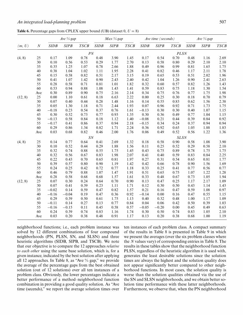
An integrated load-planning problem 507
Table 6. Percentage gaps from CPLEX upper bound (UB) (dataset 0, U = 8)
Ave % gap Max % gap Ave time (seconds) Ave % gap
(m, U) N SIDB SIPB TSCB SIDB SIPB TSCB SIDB SIPB TSCB SIDB SIPB TSCB
PN PLSN(4, 8) 25 0.17 1.09 0.78 0.48 3.90 1.45 0.17 0.54 0.70 0.48 1.16 2.69
30 0.10 0.56 0.53 0.29 1.77 2.70 0.13 0.58 0.80 0.29 2.10 2.1035 0.35 1.25 1.07 0.78 2.66 1.88 0.49 0.96 0.99 0.81 1.65 1.7540 0.38 1.04 1.02 1.11 1.95 2.28 0.41 0.82 0.46 1.17 2.11 1.7845 0.15 0.58 0.82 0.51 2.17 3.15 0.19 0.65 0.53 0.51 2.02 1.9650 0.41 1.07 1.42 0.90 2.43 2.40 0.42 1.04 1.26 0.90 2.41 2.6355 0.28 0.58 0.71 0.81 1.01 1.82 0.32 0.60 0.57 0.82 1.26 1.4360 0.53 0.94 0.88 1.08 1.43 1.41 0.59 0.83 0.75 1.18 1.30 1.54
Ave 0.30 0.89 0.90 0.75 2.16 2.14 0.34 0.75 0.76 0.77 1.75 1.98(12, 8) 25 0.00 1.10 0.61 0.18 6.63 2.22 0.00 0.25 0.30 0.18 0.70 0.79
30 0.07 0.40 0.44 0.28 1.48 1.16 0.14 0.55 0.83 0.62 1.56 2.3835 0.05 1.30 1.18 0.71 2.44 1.93 0.07 0.96 0.92 0.71 1.73 1.7540 −0.18 0.23 0.54 0.37 0.76 1.61 −0.13 0.30 0.30 0.40 1.07 1.1545 0.30 0.52 0.73 0.77 0.93 1.35 0.30 0.36 0.49 0.77 1.04 1.1550 −0.13 0.58 0.84 0.18 1.12 1.40 −0.08 0.21 0.44 0.39 0.84 0.9255 −0.17 0.41 0.86 0.37 0.94 2.18 −0.15 0.34 0.24 0.37 0.94 0.9460 0.29 0.86 1.34 0.82 1.71 2.24 0.36 0.92 0.65 1.05 1.88 1.83
Ave 0.03 0.68 0.82 0.46 2.00 1.76 0.06 0.49 0.52 0.56 1.22 1.36
SN SLSN(4, 8) 25 0.14 0.77 0.64 0.41 2.69 1.32 0.18 0.58 0.90 0.58 1.08 3.90
30 0.10 0.52 0.44 0.29 1.88 1.56 0.11 0.25 0.52 0.29 0.58 2.1035 0.32 0.74 0.88 0.55 1.75 1.45 0.43 0.75 0.89 0.78 1.75 1.7540 0.32 0.56 0.67 0.83 1.98 2.07 0.41 0.40 0.59 0.83 0.84 2.2545 0.22 0.43 0.70 0.65 0.81 1.97 0.27 0.31 0.54 0.65 0.81 1.7750 0.39 0.57 0.80 0.90 1.19 1.42 0.42 0.66 0.78 0.90 1.56 1.6955 0.24 0.25 0.42 0.72 0.77 1.18 0.33 0.25 0.41 0.77 0.56 0.7760 0.46 0.79 0.88 1.07 1.47 1.91 0.51 0.65 0.75 1.07 1.22 1.28
Ave 0.28 0.58 0.68 0.68 1.57 1.61 0.33 0.48 0.67 0.73 1.05 1.94(12, 8) 25 0.07 0.30 0.24 0.64 0.70 0.90 0.13 0.47 0.25 1.17 2.17 1.09
30 0.07 0.41 0.39 0.23 1.11 1.71 0.12 0.30 0.50 0.43 1.14 1.4335 −0.02 0.14 0.59 0.47 0.82 1.57 0.21 0.16 0.47 0.59 1.08 0.9740 −0.16 −0.04 0.19 0.47 0.36 0.92 −0.14 0.00 0.16 0.47 0.55 1.1545 0.29 0.39 0.50 0.61 1.75 1.13 0.40 0.32 0.48 1.00 1.17 1.0950 −0.11 0.14 0.27 0.13 0.77 0.84 0.04 0.06 0.42 0.50 0.39 1.0355 −0.16 −0.15 0.11 0.45 0.58 0.57 −0.05 −0.20 0.00 0.45 0.49 0.6360 0.24 0.39 0.74 0.83 1.16 1.74 0.30 0.50 0.74 0.83 1.05 2.10
Ave 0.03 0.20 0.38 0.48 0.91 1.17 0.13 0.20 0.38 0.68 1.00 1.19
neighborhood functions; i.e., each problem instance wassolved by 12 different combinations of four compoundneighborhoods (PN, PLSN, SN, and SLSN) and threeheuristic algorithms (SIDB, SIPB, and TSCB). We notethat our objective is to compare the 12 approaches relativeto each other using the same base solution, which is, for agiven instance, indicated by the best solution after applyingall 12 approaches. In Table 8, as “Ave % gap,” we providethe average of the percentage gaps from the best obtainedsolution (out of 12 solutions) over all ten instances of aproblem class. Obviously, the lower percentages indicate abetter performance of a method–neighborhood functioncombination in providing a good quality solution. As “Avetime (secends),” we report the average solution times over
ten instances of each problem class. A compact summaryof the results in Table 8 is presented in Table 9 in whichwe present the averages (over the six problem classes wherethe N values vary) of corresponding entries in Table 8. Theresults in these tables show that the neighborhood functionPLSN, regardless of the heuristic algorithm it is used with,generates the least desirable solutions since the solutiontimes are always the highest and the solution quality doesnot appear significantly better compared to other neigh-borhood functions. In most cases, the solution quality isworse than the solution qualities obtained via the use ofthe SN and SLSN neighborhoods, and we obtain better so-lution time performance with these latter neighborhoods.Furthermore, we observe that, when the PN neighborhood

Tab
le7.
Sum
mar
yof
over
alla
vera
ges
for
low
er(L
B)
and
uppe
r(U
B)
boun
dga
psan
dru
nti
mes
(dat
aset
1)
Ave
%ga
p-L
BM
ax%
gap
-LB
Ave
%ga
p-U
BM
ax%
gap
-UB
Ave
tim
e(s
econ
ds)
(M,U
)S
IDB
SIP
BT
SC
BS
IDB
SIP
BT
SC
BS
IDB
SIP
BT
SC
BS
IDB
SIP
BT
SC
BS
IDB
SIP
BT
SC
B
(4,4
)P
N3.
343.
794.
165.
756.
257.
070.
460.
891.
251.
291.
682.
701.
942.
710.
49P
LSN
3.40
3.61
3.87
5.77
6.13
6.13
0.52
0.72
0.98
1.32
1.59
2.28
9.85
9.13
3.14
SN3.
293.
373.
715.
555.
635.
910.
410.
490.
821.
101.
381.
973.
858.
651.
21SL
SN3.
413.
403.
635.
755.
645.
970.
520.
520.
741.
331.
511.
715.
8113
.00
1.90
(4,8
)P
N2.
493.
103.
125.
747.
206.
680.
300.
890.
900.
752.
162.
144.
314.
360.
80P
LSN
2.54
2.96
2.96
5.74
6.55
6.61
0.34
0.75
0.76
0.77
1.75
1.98
27.3
919
.21
8.33
SN2.
472.
782.
885.
756.
406.
430.
280.
580.
680.
681.
571.
616.
5018
.95
2.25
SLSN
2.53
2.68
2.88
5.80
6.13
6.75
0.33
0.48
0.67
0.73
1.05
1.94
14.9
031
.75
4.21
(12,
4)P
N4.
815.
226.
096.
927.
289.
58−0
.09
0.31
1.13
0.83
1.49
3.23
0.48
1.09
0.01
PL
SN4.
925.
175.
376.
967.
367.
320.
020.
260.
450.
981.
341.
573.
933.
240.
88SN
4.74
4.74
5.17
6.82
6.68
7.36
−0.1
6−0
.16
0.25
0.64
1.05
1.59
1.35
2.58
0.34
SLSN
4.85
4.69
5.08
6.93
6.8
7.22
−0.0
5−0
.20
0.17
0.79
0.97
1.47
2.00
3.75
0.45
(12,
8)P
N5.
526.
206.
3410
.59
11.5
211
.35
0.03
0.68
0.82
0.46
2.00
1.76
0.96
1.26
0.15
PL
SN5.
556.
006.
0310
.66
11.4
010
.95
0.06
0.49
0.52
0.56
1.22
1.36
7.20
5.53
2.53
SN2.
472.
782.
885.
756.
406.
430.
280.
580.
680.
681.
571.
616.
5018
.95
2.25
SLSN
2.53
2.68
2.88
5.80
6.13
6.75
0.33
0.48
0.67
0.73
1.05
1.94
14.9
031
.75
4.21
508
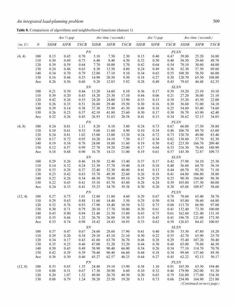
An integrated load-planning problem 509
Table 8. Comparison of algorithms and neighborhood functions (dataset 1)
Ave % gap Ave time (seconds) Ave % gap Ave time (seconds)
(m, U) N SIDB SIPB TSCB SIDB SIPB TSCB SIDB SIPB TSCB SIDB SIPB TSCB
PN PLSN(4, 4) 100 0.15 0.45 0.70 5.10 7.50 2.30 0.15 0.40 0.47 39.80 25.20 16.80
110 0.30 0.69 0.75 6.40 8.40 4.30 0.32 0.50 0.40 56.50 29.60 49.70120 0.39 0.59 0.64 7.70 10.00 5.70 0.42 0.64 0.54 70.10 30.60 44.00130 0.24 0.46 0.65 8.30 13.50 4.80 0.24 0.49 0.36 82.30 57.50 69.60140 0.34 0.70 0.79 12.80 17.10 9.10 0.34 0.65 0.55 108.50 58.50 86.00150 0.16 0.44 0.55 14.90 20.50 9.30 0.18 0.27 0.38 120.70 65.50 108.00Ave 0.26 0.56 0.68 9.20 12.83 5.92 0.28 0.49 0.45 79.65 44.48 62.35
SN SLSN100 0.21 0.39 0.44 13.20 14.60 8.10 0.36 0.17 0.39 19.20 23.10 10.10110 0.39 0.20 0.43 18.20 25.30 17.10 0.44 0.06 0.21 27.20 38.00 21.10120 0.42 0.26 0.55 24.20 24.00 13.90 0.55 0.15 0.58 35.20 43.50 22.00130 0.26 0.33 0.51 26.60 29.40 19.50 0.30 0.16 0.30 36.60 51.00 34.10140 0.39 0.14 0.38 37.30 55.90 41.30 0.48 0.18 0.25 54.80 93.40 74.60150 0.26 0.23 0.37 42.10 41.80 23.60 0.30 0.17 0.30 58.70 63.90 42.40Ave 0.32 0.26 0.45 26.93 31.83 20.58 0.41 0.15 0.34 38.62 52.15 34.05
PN PLSN(4, 8) 100 0.24 0.81 1.11 8.20 8.10 3.80 0.24 0.73 0.67 66.00 17.50 38.80
110 0.10 0.61 0.53 9.60 11.60 4.90 0.10 0.54 0.46 106.70 89.70 63.60120 0.24 0.81 1.02 15.00 13.00 13.20 0.24 0.72 0.73 120.70 49.00 83.40130 0.17 0.72 0.95 16.20 14.10 7.50 0.17 0.54 0.62 138.60 37.70 82.30140 0.19 0.54 0.78 24.00 18.80 11.60 0.19 0.50 0.42 223.50 166.70 209.40150 0.12 0.57 0.99 27.70 19.20 25.00 0.17 0.64 0.53 216.30 76.60 180.90Ave 0.18 0.68 0.90 16.78 14.13 11.00 0.19 0.61 0.57 145.30 72.87 109.73
SN SLSN100 0.29 0.26 0.46 18.50 32.40 13.40 0.37 0.17 0.42 37.90 54.10 25.30110 0.14 0.32 0.24 21.30 37.70 19.40 0.18 0.18 0.40 36.60 64.70 38.10120 0.33 0.28 0.37 32.40 52.30 48.00 0.41 0.13 0.44 60.70 92.30 71.10130 0.23 0.42 0.63 35.70 49.30 22.60 0.26 0.18 0.41 64.80 106.80 38.80140 0.22 0.26 0.34 48.50 70.80 89.10 0.29 0.29 0.25 90.30 184.00 98.30150 0.22 0.43 0.41 55.10 85.70 43.80 0.28 0.24 0.39 103.80 157.30 80.00Ave 0.24 0.33 0.41 35.25 54.70 39.38 0.30 0.20 0.38 65.68 109.87 58.60
PN PLSN(12, 4) 100 0.27 0.75 1.01 12.80 11.80 4.60 0.29 0.67 0.78 70.60 65.40 38.70
110 0.29 0.63 0.88 11.60 14.40 5.50 0.29 0.50 0.54 85.00 58.60 64.80120 0.32 0.76 0.93 17.90 18.40 10.50 0.32 0.75 0.80 113.70 66.90 97.00130 0.30 0.71 0.79 20.10 17.70 10.00 0.30 0.61 0.41 132.40 73.30 100.00140 0.43 0.90 0.94 21.40 21.50 15.80 0.43 0.75 0.61 162.60 121.40 131.10150 0.35 0.66 1.32 26.70 26.80 19.30 0.35 0.45 0.41 196.70 121.00 173.50Ave 0.33 0.74 0.98 18.42 18.43 10.95 0.33 0.62 0.59 126.83 84.43 100.85
SN SLSN100 0.37 0.47 0.67 24.60 28.60 17.90 0.41 0.40 0.50 33.50 47.80 18.20110 0.29 0.20 0.34 29.10 45.10 21.10 0.30 0.22 0.55 42.70 65.90 25.70120 0.34 0.17 0.43 41.60 63.70 36.70 0.48 0.28 0.29 55.40 107.20 50.40130 0.35 0.25 0.46 47.00 51.20 33.20 0.44 0.30 0.48 65.00 79.60 46.50140 0.50 0.43 0.49 58.90 90.40 66.00 0.54 0.26 0.54 77.10 114.70 70.70150 0.42 0.29 0.39 70.40 96.40 66.60 0.44 0.18 0.34 99.60 137.60 89.50Ave 0.38 0.30 0.46 45.27 62.57 40.25 0.44 0.27 0.45 62.22 92.13 50.17
PN PLSN(12, 8) 100 0.33 0.85 1.35 24.40 19.10 13.90 0.38 1.10 0.91 185.50 63.30 194.40
110 0.08 0.51 0.67 17.30 20.90 6.60 0.10 0.32 0.46 179.90 282.00 91.20120 0.20 1.07 1.32 49.80 26.70 49.50 0.20 0.65 0.79 316.80 177.00 534.30130 0.08 0.79 1.24 38.20 25.50 19.20 0.11 0.73 0.66 254.90 164.90 221.80
(Continued on next page)

510 Uster and Agrahari
Table 8. Comparison of algorithms and neighborhood functions (dataset 1) (Continued)
Ave % gap Ave time (seconds) Ave % gap Ave time (seconds)
(m, U) N SIDB SIPB TSCB SIDB SIPB TSCB SIDB SIPB TSCB SIDB SIPB TSCB
140 0.04 0.48 0.64 38.50 35.50 16.70 0.05 0.32 0.38 355.40 454.50 294.40150 0.22 0.71 1.20 60.00 41.30 30.50 0.24 0.73 0.52 419.60 314.90 550.20Ave 0.16 0.74 1.07 38.03 28.17 22.73 0.18 0.64 0.62 285.35 242.77 314.38
SN SLSN100 0.44 0.21 0.33 45.50 93.60 29.20 0.51 0.18 0.55 97.60 137.40 57.00110 0.15 0.26 0.45 33.20 70.10 22.40 0.20 0.32 0.32 59.40 123.00 68.60120 0.23 0.24 0.36 74.70 167.70 69.90 0.29 0.17 0.31 169.80 367.80 137.70130 0.17 0.30 0.28 66.60 110.40 72.80 0.33 0.36 0.41 112.80 189.70 90.80140 0.09 0.34 0.44 72.00 131.10 105.40 0.17 0.28 0.33 122.20 246.50 139.20150 0.27 0.20 0.38 109.10 196.90 105.00 0.38 0.30 0.21 203.50 363.80 121.60Ave 0.23 0.26 0.37 66.85 128.30 67.45 0.31 0.27 0.35 127.55 238.03 102.48
function is employed, the solution times are significantlybetter with each of the three heuristic algorithms and, atthe same time, the solution qualities are at easily accept-able levels as illustrated by the majority of the results wherethe average percentage gaps are below 1.0%. On the otherhand, from the heuristic algorithms perspective, the SIPBand SIDB appear to perform better than TSCB as theyprovide lower average percentage gaps. Especially, the com-bination of SIPB and the neighborhood functions SN orSLSN perform exceptionally well in terms of solution qual-ity as measured by the number of times they provide thebest solution but not in terms of solution times as notedabove.
Since, based on the dataset 1 results, we observe thatthe adoption of our proposed compound neighborhoodfunctions lead to faster algorithms without serious com-
Table 9. Summary of comparisons (dataset 1)
Ave % gap Ave time (seconds)
(M, U) SIDB SIPB TSCB SIDB SIPB TSCB
(4, 4) PN 0.26 0.56 0.68 9.20 12.83 5.92PLSN 0.28 0.49 0.45 79.65 44.48 62.35SN 0.32 0.26 0.45 26.93 31.83 20.58SLSN 0.41 0.15 0.34 38.62 52.15 34.05
(4, 8) PN 0.18 0.68 0.90 16.78 14.13 11.00PLSN 0.19 0.61 0.57 145.30 72.87 109.73SN 0.24 0.33 0.41 35.25 54.70 39.38SLSN 0.30 0.20 0.38 65.68 109.87 58.60
(12, 4) PN 0.33 0.74 0.98 18.42 18.43 10.95PLSN 0.33 0.62 0.59 126.83 84.43 100.85SN 0.38 0.30 0.46 45.27 62.57 40.25SLSN 0.44 0.27 0.45 62.22 92.13 50.17
(12, 8) PN 0.16 0.74 1.07 38.03 28.17 22.73PLSN 0.18 0.64 0.62 285.35 242.77 314.38SN 0.23 0.26 0.37 66.85 128.30 67.45SLSN 0.31 0.27 0.35 127.55 238.03 102.48
promise in solution quality, in the last stage of our numeri-cal study we concentrated on comparing only the heuristicalgorithms, SIDB, SIPB, and TSCB, while employing theneighborhood function PN in each one. We considered theeven larger problem instances provided by dataset 2.The results are summarized in Table 10 in which we observethat the TSCB performs best in terms of solution qualitywhile the TSCB and SIPB algorithms present very simi-lar performances with large U and M. Interestingly, TSCBgenerally perform better in these large instance; however, itssolution time is significantly high as well. Although SIPBdoes not perform as well as TSCB, its performance is alsovery satisfactory in general as it provides less than a 0.5%gap on average from the best available solution. Further-more, solution times with the SIPB are highly favorable.Thus, it appears that the SIPB algorithm, implemented byemploying the neighborhood function PN, is a promisingapproach, both in terms of solution quality and solutiontime.
7. Concluding remarks
In this article, we considered a load planning-problemwith explicit consideration of consolidating smaller loadsinto capacitated TLs as found, for example, in generalfreight forwarding applications. A commodity is trans-ported between its origin and destination either directlyor by following a route that visits centers where it is con-solidated/deconsolidated with other loads. We provided acompact mathematical formulation for the problem of theleast-cost commodity flow with the TL consolidation con-siderations addressed explicitly. We observed that a specialcase of the model resembles a capacitated location problemwith single sourcing, and the instances that we are inter-ested in imply very large-scale and challenging instancesof this problem due to a large number of customers (com-modities) and an even larger number of potential locations.

An integrated load-planning problem 511
Table 10. Comparing SIDB, SIPB, and TSCB using the neighborhood function PN (dataset 2)
Ave % gap Ave time (seconds)
(M, U) N SIDB SIPB TSCB SIDB SIPB TSCB
(4, 4) 500 1.03 0.28 0.09 333.90 348.10 490.70550 0.73 0.35 0.06 475.90 301.30 701.00600 0.92 0.32 0.01 418.30 320.00 758.50650 0.80 0.28 0.01 565.60 336.60 553.80700 0.81 0.24 0.02 781.00 475.80 1197.00750 0.76 0.10 0.13 629.00 806.60 1493.00800 0.70 0.32 0.02 933.50 541.10 1884.80850 1.20 0.31 0.03 1608.40 1906.90 3272.40900 0.89 0.17 0.04 1208.10 1109.10 1929.10950 1.10 0.38 0.02 1352.40 1496.60 6714.201000 1.24 0.55 0.00 1865.70 2115.30 9154.20Ave 0.93 0.30 0.04 924.71 887.04 2558.97
(4, 12) 500 0.72 0.13 0.23 436.80 384.90 561.30550 0.87 0.24 0.07 526.10 466.30 867.10600 0.77 0.19 0.24 641.70 623.30 853.80650 0.71 0.24 0.08 1026.90 802.30 1242.70700 0.64 0.15 0.13 1107.50 870.70 1442.30750 0.67 0.17 0.09 1298.50 1076.90 1885.80800 0.37 0.16 0.10 1173.80 1009.90 1980.40850 0.52 0.20 0.14 1126.50 1163.50 2092.90900 0.52 0.28 0.16 1763.00 1096.70 2330.20950 0.53 0.19 0.11 2180.20 1670.10 3641.501000 0.38 0.20 0.17 2232.80 2002.50 3438.40Ave 0.61 0.20 0.14 1228.53 1015.19 1848.76
(4, 8) 500 0.34 0.18 0.23 495.00 400.70 953.80550 0.34 0.30 0.12 697.80 387.00 1018.40600 0.45 0.44 0.14 454.40 282.40 979.80650 0.31 0.29 0.00 881.60 431.80 1243.90700 0.54 0.47 0.10 1095.40 439.30 2141.70750 0.26 0.22 0.42 746.90 861.50 1263.60800 0.48 0.41 0.16 1163.60 606.60 2029.90850 0.57 0.33 0.18 2261.90 1109.50 3240.70900 0.40 0.31 0.11 1497.30 1452.80 2303.40950 0.36 0.52 0.07 1846.00 758.10 3784.601000 0.61 0.43 0.07 2419.10 1102.40 10702.10Ave 0.42 0.35 0.15 1232.64 712.01 2696.54
(12, 8) 500 0.44 0.33 0.28 706.10 598.70 851.30550 0.29 0.12 0.47 941.20 616.70 775.70600 0.24 0.28 0.18 1164.10 729.60 966.80650 0.26 0.20 0.23 1675.50 865.90 1325.40700 0.27 0.48 0.08 1894.60 965.00 1787.10750 0.43 0.30 0.13 2093.00 1156.30 2534.10800 0.11 0.48 0.24 1814.40 1727.30 3416.20850 0.20 0.46 0.23 1787.90 1563.60 2679.30900 0.13 0.52 0.38 2764.70 1973.00 3226.50950 0.14 0.22 0.37 3673.70 2248.60 4344.101000 0.15 0.37 0.31 3404.80 2460.90 4015.00Ave 0.24 0.34 0.26 1992.73 1355.05 2356.50
Overall Ave 0.55 0.30 0.15 1344.65 992.32 2365.19
To develop heuristic algorithms, we first proposed fourdistinct compound neighborhood structures. A compoundneighborhood involves two main components, LC and CC,which combine various simple neighborhood functions in
a certain way for the purpose of generating a neighboringsolution. Given the complexity of efficient solution repre-sentation required in a heuristic framework, our compoundneighborhood functions give us the opportunity to search
512 Uster and Agrahari
the solution space efficiently using a branching strategy thatrelies on the LC component, which is the common compo-nent in all four compound neighborhoods. Furthermore,the components provide a means for instilling intensifica-tion (via CC) and diversification (via LC) characteristicsinto the algorithms.
Our extensive computational study using four differentdatasets representing varying problem sizes revealed thatthe serial-type compound neighborhood functions (SNand SLSN) perform better in terms of solution quality,although they require the longest solution time on aver-age. On the other hand, the parallel-type function withlocal search (PLSN) performs poorly in terms of both so-lution quality and time. However, the neighborhood func-tion PN performs best in terms of solution time and verysatisfactorily (most of the time close to the SN and SLSNperformance) in solution quality. These results are gener-ally consistent independent of the heuristic algorithm withwhich they are used. From the algorithmic perspective, weobserved that the TSCB provides better solutions, espe-cially for the large instances, but at the expense of solutiontime. On the other hand, the SIPB performs very satisfac-torily in terms of solution quality and is the best in termsof solution time, especially for large instances. We also notethat, although the SIDB performs well with small-sizedproblems, its performance diminishes with larger-sized in-stances where the solution space grows significantly and themeta-heuristic-based approaches become more effective.
Finally, our heuristics with both parallel and serial neigh-borhoods are run on single processor PCs. However, anadvantage of heuristics with parallel compound neighbor-hoods, CC-PN and CC-PLSN, is that they can be effi-ciently run on parallel processors to improve run timesdramatically.
This study can be extended in various ways in both theproblem domain and the application of solution method-ologies. Some of our current efforts include both frontsin the following areas. The problem that we consider canbe seen as a subproblem for the case where we are in-terested in determining the locations of the consolidationand deconsolidation centers as well. Furthermore, moregeneral cost functions that incorporate other forms ofeconomies-of-scale and -distance characteristics of trans-portation for the transfer links can be incorporated into themodel. Finally, it is worthwhile to note that our proposedcompound neighborhoods, branching strategies, and theheuristic algorithms can be employed in solving variousfacility location and other partitioning-based optimizationproblems.
References
Aarts, E., Korst, J.H.M. and van Laarhoven, P.J.M. (1997) Simulatedannealing, in Local Search in Combinatorial Optimization, Aarts, E.and Lenstra, J.K. (eds), Wiley, New York, pp. 91–120.
Agar, M.C. and Salhi, S. (1998) Lagrangian heuristics applied to avariety of large capacitated plant location problems. Journal of theOperational Research Society, 49(10), 1072–1084.
Ahuja, R.K., Orlin, J.B., Pallottino, S., Scaparra, M.P. and Scutella, M.G.(2004) A multi-exchange heuristic for the single-source capacitatedfacility location problem. Management Science, 50(6), 749–760.
Amiri, A. and Pirkul, H. (1997) New formulation and relaxation to solvea concave-cost network flow problem. Journal of Operational ResearchSociety, 48, 278–287.
Armacost, A.P., Barnhart, C., Ware, K.A. and Wilson, A.M. (2004) UPSoptimizes its air network. Interfaces, 34(1), 15–25.
Balakrishnan, A. and Graves, S.C. (1989) A composite algorithm for aconcave-cost network flow problem. Networks, 19, 175–202.
Barcelo, J. and Casanovas, J. (1984) A heuristic Lagrangian algorithmfor the capacitated plant location problem. European Journal of Op-erational Research, 15(2), 212–226.
Barnhart, C., Krishnan, N., Kim, D. and Ware, K. (2002) Networkdesign for express shipment delivery. Computational Optimization andApplications, 21(3), 239–262.
Barnhart, C. and Schneur, R.R. (1996) Air network design for expressshipment service. Operations Research, 44(6), 852–863.
Beasley, J.E. (1993) Lagrangian heuristics for location problems. Euro-pean Journal of Operational Research, 65(3), 383–399.
Budenbender, K., Grunert, T. and Sebastian, H. (2000) A hybrid tabusearch/branch-and-bound algorithm for the direct flight network de-sign problem. Transportation Science, 34(4), 364–380.
Campbell, J. F. (2005) Strategic network design for motor carriers, in Lo-gistics Systems—Design and Optimization, Langevin, A. and Riopel,D. (eds), Springer-Verlag, New York, pp. 245–278.
Cohn, A., Root, S., Wang, A. and Mohr, D. (2007) Integration of theload matching and routing problem with equipment balancing forsmall package carriers. Transportation Science, 41(2), 238–252.
Cortinhal, M.J. and Captivo, M.E. (2003) Upper and lower bounds forthe single source capacitated location problem. European Journal ofOperational Research, 151(2), 333–351.
Delmaire, H. et al. (1999) Reactive GRASP and tabu search basedheuristics for the single source capacitated plant location problem.INFOR, 37, 194–225.
Diaz, J.A. and Fernandez, E. (2002) A branch-and-price algorithm forthe single source capacitated plant location problem. Journal of theOperational Research Society, 53, 728–740.
Glover, F. and Laguna, M. (1997) Tabu Search, Kluwer, Norwell, MA.Grunert, T. and Sebastian, H. (2000) Planning models for long-haul op-
erations of postal and express shipment companies. European Journalof Operational Research, 122(2), 289–309.
Hansen, P. and Mladenovic, N. (2003) Variable neighborhood search,in Handbook of Metaheuristics, Glover, F. and Kochenberger, G.A.(eds), Kluwer, Norwell, MA, pp. 145–184.
Hindi, K.S. and Pienkosz, K. (1999) Efficient solution of large scale,single-source, capacitated plant location problems. Journal of theOperational Research Society, 50(3), 268–274.
Holmberg, K., Ronnqvist, M. and Yuan, D. (1999) An exact algorithmfor the capacitated facility location problems with single sourcing.European Journal of Operational Research, 113(3), 544–559.
Jarrah, A.I., Johnson, E. and Neubert, L.C. (2008) Large-scale less-than-truckload service network design. Operations Research, 57, 609–625.
Klincewicz, J.G. and Luss, H. (1986) A Lagrangian relaxation heuristicfor capacitated facility location with single-source constraints. Journalof the Operational Research Society, 37(5), 495–500.
Lamar, B.W. and Sheffi, Y. (1987) An implicit enumeration method forLTL network design. Transportation Research Record, 1120, 1–11.
Lapierre, S.D., Ruiz, A.B. and Soriano, P. (2004) Designing distributionnetworks: formulations and solution heuristic. Transportation Science,38(2), 174–187.
Leung, J.M.Y., Magnanti, T.L. and Singhal, V. (1990) Routing in point-to-point delivery systems: formulations and solution heuristics. Trans-portation Science, 24(4), 245–260.

An integrated load-planning problem 513
Lourenco, H.R., Martin, O.C. and Stutzle, T. (2003) Iterated local search,in Handbook of Metaheuristics, Glover, F. and Kochenberger, G.A.(eds), Kluwer, Norwell, MA, pp. 321–353.
Muriel, A. and Munshi, F.N. (2003) Capacitated multicommodity net-work flow problems with piecewise linear concave costs. IIE Transac-tions, 36, 683–696.
Neebe, A.W. and Rao, M.R. (1983) An algorithm for the fixed-charge as-signing users to sources problem. Journal of the Operational ResearchSociety, 34(11), 1107–1113.
Pirkul, H. (1987) Efficient algorithms for the capacitated concentratorlocation problem. Computers & Operations Research, 14(3), 197–208.
Powell, W.B. (1986) A local improvement heuristics for the design ofless-than-truckload motor carrier networks. Transportation Science,20, 246–257.
Powell, W.B. and Sheffi, Y. (1983) The load planning problem of mo-tor carriers: problem description and a proposed solution approach.Transportation Research Part A: Policy and Practice, 17, 471–480.
Powell, W.B. and Sheffi, Y. (1989) Design and implementation of aninteractive optimization system for network design in the motor carrierindustry. Operations Research, 37(1), 12–29.
Root, S. and Cohn, A. (2008) A novel modeling approach for expresspackage carrier planning. Naval Research Logistics, 55(7), 670–683.
Sait, S.M. and Youssef, H. (1999) Iterative Computer Algorithms with Ap-plications in Engineering: Solving Combinatorial Optimization Prob-lems, IEEE Computer Society, Los Alamitos, CA.
Sridharan, R. (1993) A Lagrangian heuristic for the capacitated plantlocation problem with single source constraints. European Journal ofOperational Research, 66(3), 305–312.
Biographies
Halit Uster is an Associate Professor in the Department of Industrial andSystems Engineering at Texas A&M University. He holds a Ph.D. in Man-agement Science/Systems from McMaster University, Ontario, Canada.His research interests are in the areas of logistics, design of networkedsystems, and applied optimization. His publications appeared in Comput-ers and Operations Research, European Journal of Operational Research,Interfaces, IIE Transactions, Naval Research Logistics and TransportationScience, among others. He is an Associate Editor for IIE Transactionsand a member of IIE and INFORMS.
Homarjun Agrahari is a Senior Operations Research Specialist in the De-partment of Service Design & Performance at BNSF Railway Company.At BNSF, he is involved in design, development, and implementation ofdecision systems that address network design, scheduling, and reschedul-ing problems arising in freight train networks. He received his Ph.D. inIndustrial Engineering from the Department of Industrial and SystemsEngineering at Texas A&M University. His research interests includedeveloping modeling and exact/meta-heuristic solution approaches fornetwork optimization problems arising in networked systems such astransportation, logistics, and supply chain networks. He obtained hismaster’s in Computer Integrated Manufacturing and bachelor’s in Me-chanical Engineering, both from the Indian Institute of Technology,Bombay, India. He is a member of IIE and INFORMS. He receivedthe INFORMS Judith Liebman Award in October 2008.