an integrated cvar and real options approach to ... · an integrated cvar and real options approach...

209

Reihe Ökonomie

Economics Series

An Integrated CVaR and Real Options Approach to

Investments in the Energy Sector

Ines Fortin, Sabine Fuss, Jaroslava Hlouskova, Nikolay Khabarov, Michael Obersteiner, Jana Szolgayova

209

Reihe Ökonomie

Economics Series

An Integrated CVaR and Real Options Approach to

Investments in the Energy Sector

Ines Fortin, Sabine Fuss, Jaroslava Hlouskova, Nikolay Khabarov, Michael Obersteiner, Jana Szolgayova

May 2007

Institut für Höhere Studien (IHS), Wien Institute for Advanced Studies, Vienna

Contact: Ines Fortin IHS, Stumpergasse 56, 1060 Vienna, Austria

: 43/1/59991-165 Email: [email protected] Sabine Fuss University of Maastricht/UNU-Merit Keizer Karelplein 19, 6211 TC Maastricht, The Netherlands

: +31/43/3884-430 email: [email protected] Jaroslava Hlouskova IHS, Stumpergasse 56, 1060 Vienna, Austria

: 43/1/59991-142 email: [email protected] Nikolay Khabarov International Institute for Applied Systems Analysis (IIASA) 2361 Laxenburg, Austria

: +43/2236/807-346 email: [email protected] Michael Obersteiner International Institute for Applied Systems Analysis (IIASA) 2361 Laxenburg, Austria

: +43/2236/807-460 email: [email protected] Jana Szolgayova International Institute for Applied Systems Analysis (IIASA) 2361 Laxenburg, Austria

: +43/2236/807-349 email: [email protected]

Founded in 1963 by two prominent Austrians living in exile – the sociologist Paul F. Lazarsfeld and the economist Oskar Morgenstern – with the financial support from the Ford Foundation, the Austrian Federal Ministry of Education and the City of Vienna, the Institute for Advanced Studies (IHS) is the firstinstitution for postgraduate education and research in economics and the social sciences in Austria.The Economics Series presents research done at the Department of Economics and Finance andaims to share “work in progress” in a timely way before formal publication. As usual, authors bear fullresponsibility for the content of their contributions. Das Institut für Höhere Studien (IHS) wurde im Jahr 1963 von zwei prominenten Exilösterreichern –dem Soziologen Paul F. Lazarsfeld und dem Ökonomen Oskar Morgenstern – mit Hilfe der Ford-Stiftung, des Österreichischen Bundesministeriums für Unterricht und der Stadt Wien gegründet und ist somit die erste nachuniversitäre Lehr- und Forschungsstätte für die Sozial- und Wirtschafts-wissenschaften in Österreich. Die Reihe Ökonomie bietet Einblick in die Forschungsarbeit der Abteilung für Ökonomie und Finanzwirtschaft und verfolgt das Ziel, abteilungsinterne Diskussionsbeiträge einer breiteren fachinternen Öffentlichkeit zugänglich zu machen. Die inhaltlicheVerantwortung für die veröffentlichten Beiträge liegt bei den Autoren und Autorinnen.

Abstract

The objective of this paper is to combine a real options framework with portfolio optimization techniques and to apply this new framework to investments in the electricity sector. In particular, a real options model is used to assess the adoption decision of particular technologies under uncertainty. These technologies are coal-fired power plants, biomass-fired power plants and onshore wind mills, and they are representative of technologies based on fossil fuels, biomass and renewables, respectively. The return distributions resulting from this analysis are then used as an input to a portfolio optimization, where the measure of risk is the Conditional Value-at-Risk (CVaR).

Keywords Portfolio optimization, CVaR, climate change policy, uncertainty, real options, electricity, investments

JEL Classification C61, D81, D92, G11, Q4, Q56, Q58

Comments Ines Fortin, Jaroslava Hlouskova, and Michael Obersteiner gratefully acknowledge financial supportfrom the Austrian National Bank (Jubiläumsfonds Grant No. 11883). AT IIASA this work was carried out in the framework of the project "Bewertungsmodelle für zukünftige Energiecluster unter Markt-,Technologie- und Politikunsicherheit - Fallstudie Biomasse" funded by FFG (Österreichische Forschungsförderungsgesellschaft), Vienna. Sabine Fuss, Nikolay Khabarov, Michael Obersteiner and Jana Szolgayova are grateful for the financial support of FFG.

Contents

1 Introduction 1

2 The Real Options Model 5 2.1 The Framework ........................................................................................................... 5 2.2 The Technologies and the Data .................................................................................. 9 2.3 Results of the Real Options Model ........................................................................... 10

3 CVaR-based Portfolio Optimization 15 3.1 CVaR as a Risk Measure .......................................................................................... 15 3.2 Portfolio Optimization: Minimizing Risk ..................................................................... 17 3.3 Portfolio Optimization: Maximizing Returns .............................................................. 18 3.4 Results of the CVaR Approach ................................................................................. 19 3.5 Mean-variance versus CVaR .................................................................................... 23

4 Conclusion 27

Appendix A: Snapshots of Price Distributions for All Scenarios 29

Appendix B: Real Options Output for Investing and Switching 30

Appendix C: Definitions of Copulas and Related Concepts 33

References 35

1 Introduction

Uncertainty about the cause-and-effect relationships of anthropogenic emissions, global warm-ing and a large number of (possibly irreversible) effects impedes effective policy making andposes considerable uncertainties to investors in addition to the common uncertainties origi-nating from fluctuations in input and output prices. If investors cannot be sure about futureclimate change policy measures, they will typically not invest in environmentally friendly,expensive technologies. Therefore, it is important not only to concentrate on variability inreturns from market-driven fluctuations in prices, but also to take into account the uncer-tainties emanating from the policy making process. In this paper we will focus on investmentplanning in the electricity sector, since the generation of electricity contributes significantlyto total CO2 emissions and has therefore been a major area of concern to policymakers.

The electricity sector is marked not only by uncertainties surrounding investment andproduction decisions, but also by irreversibility due to the large sunk costs involved in invest-ment in generation equipment and the flexibility to postpone investments to a later point intime during the planning horizon. Therefore, we think that real options modeling is a suitableapproach for investment planning. Originally developed for valuing financial options in theseventies (Black and Scholes, 1973, and Merton, 1973), economists soon realized that optionpricing also provided considerable insight into decision-making concerning capital investment.Hence the term “real” options. Early frameworks were developed by McDonald and Siegel(1986), Pindyck (1988, 1991, 1993), and Dixit and Pindyck (1994).1 The basic idea is thatstandard investment theory relying on net present value (NPV) calculations generally do notconsider the interaction between three important characteristics of investment decisions: theirreversibility of most investments, which implies that a substantial portion of the total in-vestment cost is sunk, the uncertainty surrounding the future cash flows from the investment,which can be affected by e.g. the volatility of output and input prices, and the opportunity oftiming the investment flexibly. Regarding the opportunity to defer an investment means thatwe can assign a value to waiting. In other words, investors gain more information about theuncertainty that surrounds economic decisions as time passes by. Therefore, staying flexibleby postponing decisions has an option value if the degree of uncertainty faced is big enough.This value increases if the sunk cost that has to be incurred to launch the project is high,but also in times of larger uncertainty associated with future cost or revenues. In this case itpays off to wait and see how the conditions have changed, especially if they are expected tobe rather stable afterwards.

Investment in the electricity sector has been analyzed within real options frameworksbefore. In the area of short-term planning, this work includes e.g. Tseng and Barz (2002),Hlouskova et al (2005) and Deng and Oren (2003). At the same time, a number of long-term planning frameworks have emerged. A recent example is by Fleten et al (2006), whofind that investment in power plants relying on renewable energy sources will be postponedbeyond the traditional NPV break even point when a real options approach with stochasticelectricity prices is used. With respect to uncertainty from government regulation in theelectricity sector, De Jong et al (2004) propose that real options modeling is a valuable methodto investigate how fluctuations in future emissions prices affect investment patterns. AlsoLaurikka (2004), Laurikka and Kojonen (2006), Kiriyama and Suzuki (2004), and Reedman

1For a comprehensive treatment and overview of both financial and real options theory see Trigeorgis(1996). More advanced and with several applications is Schwartz and Trigeorgis (2001).

1

et al (2006) deal with the influence of future uncertain emissions trading and with CO2

penalties within a real options setup. In these models the design of emissions trading schemesand the number of allowances that are freely distributed are main features of the overallmodel.

On the other hand, Fuss et al (2006) focus on the overall effect of uncertainty emanatingfrom climate change policy and the effect of market uncertainty, where the specific form ofemissions trading schemes is not an issue. In their framework CO2 prices can be seen as a sortof carbon tax or as the price for an allowance that has to be bought on the carbon market;CO2 prices thus add to the total cost of electricity producers. We use this same frameworkin the present paper. Sources of uncertainty are the price of CO2 and the price of electricity,which are modeled as stochastic processes. A feature of the model which is disregarded inmany other frameworks is the relation between CO2 costs and electricity prices. In our modelthis is captured by the fact that the increments of the two price processes and thus theprice processes themselves are positively correlated. In fact the use of (linear) correlation todescribe and model dependence implies a symmetric dependence structure. To capture theintuitively plausible fact that dependence may be higher in times of increasing prices thanin times of decreasing prices, more general forms of dependence modeling involving so-calledcopulas would be appropriate. Solving this is beyond the scope of our paper and will be leftfor future research.

We use a real options model to find the optimal timing of investing into carbon capture andstorage (CCS) modules in the case of coal- and biomass-fired power plants. For renewablesthe optimal installation time of the plant as such is computed. We find that the wind turbine,the basic coal plant (without CCS) and the basic biomass plant (without CCS) are all builtin the first year.

While this optimization is performed by the individual power producer, who wants to setup a new plant, large investors would typically want to invest in a portfolio of technologiesrather than concentrate on a single technology or a single chain. The contribution of thispaper is to combine portfolio optimization with the results that we derive from our real op-tions framework. In particular, we use the real options model to find the optimal investmentstrategy and its implied return distributions; the return distributions, then, can be employedas an input into the portfolio optimization. In traditional finance, the standard portfolio op-timization procedure is the mean-variance approach introduced by Markowitz (1952), wherethe portfolio variance is minimized subject to a constraint on the expected return. Risk man-agement in financial institutions, however, has started to employ another measure of risk,the Value-at-Risk (VaR), since it captures extreme – and thus dangerous – events providinginformation on the tail of a distribution. Also regulatory requirements as specified by theBasel Committee on Banking Supervision (2003, 2006) are geared towards the use of VaR.Another risk measure, which is closely related to VaR but offers additional desirable prop-erties like coherence and computational ease, is Conditional Value-at-Risk (CVaR). WhileVaR is generally better known and more widely employed, we think that CVaR is the moreappropriate measure to use. Let us define VaR and CVaR to make clear what we are talkingabout. According to Rockafellar and Uryasev (2000) the β-VaR of a portfolio is the lowestamount α such that, with probability β, the loss will not exceed α, whereas the β-CVaR isthe conditional expectation of losses above that amount α, where β is a specified probabilitylevel.2

2This (simple) definition applies only to situations where the loss distribution is continuous. For the

2

The disadvantages of VaR as opposed to CVaR relate to both usefulness in risk manage-ment and technical properties. VaR does not consider losses exceeding the threshold valuewhile CVaR does, and this information might be useful, in particular in times of financialdistress. Further, VaR is only a coherent risk measure in the sense of Artzner et al (1999)if distributions are assumed to be normal; generally, VaR is neither subadditive nor convex.CVaR, on the other hand, is always a coherent risk measure. In addition, the powerful resultsin Rockafellar and Uryasev (2000, 2002) make computational optimization of CVaR readilyaccessible. Note that, under mild technical restrictions, the minimization of VaR and CVaRand the mean-variance framework yield the same results provided that all underlying distri-butions are normal. This does not apply if the assumption of normality is violated. We willsee that both the univariate distributions and the joint distribution (copula) of the returns,which are the results from our real options procedure, do not seem to be normal in mostcases. A more detailed treatment of the difference between VaR and CVaR can be foundin Rockafellar and Uryasev (2000). To our knowledge, combining real options with portfoliooptimization using CVaR is a new approach which has not been implemented before. Somerecent literature has undertaken steps into similar directions, however.

Alesii (2005) uses VaR in combination with real options, but his aims and therefore alsohis approach are very different from ours. He acknowledges that with a real options approachdownside risk is reduced and the distribution of the expanded NPV3 is thus favorably skewed(Trigeorgis, 1996). The aim of his paper is to quantify this impact on risk. To this end heuses an extension of the model by Kulatilaka (1988) to calculate the VaR on the expandedNPV and the CFaR (the cash-flow-at-risk in each period of the planning horizon). To be moreprecise, he first derives expanded NPVs and optimal exercise thresholds for all options withbackward induction. Then, with a stochastic, mean-reverting state variable, he conductsa Monte Carlo simulation and uses the simulated time series to compute the cash flowsconsidering the optimal exercise times. Alesii (2005) calls these cash flows “controlled” cashflows and uses them to calculate the expanded NPVs, which converge to the values previouslycomputed recursively. The model results confirm that real options reduce downside risk andreshape the distribution of the expanded NPV positively: Both VaR and CFaR decreasesubstantially when options are taken into consideration. The conclusion is that real optionsdo not only enhance the value of the expanded NPV compared to the standard NPV, but italso decreases the involved risk. Alesii (2005) therefore uses VaR only as a measure of risk onthe distribution of expanded NPV and CFaR as the risk measure for cash flows in each timeperiod in order to determine the impact of including real options on the variability in NPVand cash flows. In contrast, we use CVaR instead of VaR and we employ it as a risk measurefor a portfolio optimization where the distributions resulting from real options modeling arethe input rather than the output to the (portfolio) optimization process.

The CVaR approach has been followed by a number of papers dealing with real worldrisk management, including risk management in the electricity sector. Example of such ap-plications are Unger and Luthi (2002) and Doege et al (2006); they maximize expected profitof a given power portfolio while restricting overall risk as measured by CVaR. Their modelis different from ours in various ways, however. First, the portfolio includes financial assets(contracts) as well as physical assets (production assets), where the latter consist of a num-

discrete case, definitions are more subtle, see Rockafellar and Uryasev (2002).3The expanded NPV differs from the standard NPV by the value of the option that is explicitly taken into

account in real options modeling.

3

ber of hydro storage/pump plants in the first application and a combination of a base loadgenerator (nuclear power plant) and a peaker (hydro pump storage) in the second one. Timehorizons considered are rather short – two weeks and 1 year – with the time unit being onehour. Sources of uncertainty in these models are the electricity price, the demand for elec-tricity and water inflow. Even though the framework used is not explicitly the real optionsframework, the model is quite similar except for potentially flexible times of investment inthe real options framework.

Spangardt et al (2006) present the basic idea of optimizing a power portfolio while con-straining risk in terms of CVaR, applying the results of Rockafellar and Uryasev (2000, 2002),and give a survey of related application papers. They, too, do not explicitly suggest a realoptions framework but their stochastic optimization setup is again quite similar to our realoptions analysis with the same reservation as above. The application papers referred to, how-ever, turn out – for the most part – to not apply CVaR as a measure of risk; generally risk istaken care of by introducing risk penalties in the objective function, where risk is measuredby the standard deviation. One of the applications, which is probably closest to our problem,can be found in Fichtner et al (2002). The authors use the PERSEUS-EVU model4 to max-imize expected profits by determining the optimal production portfolio, where the planninghorizon is 30 years and constraints can be set for emission levels. The paper presents a casestudy for three different scenarios of CO2 emission limits in Germany. The main results are inline with our results; the production portfolio is significantly changing depending on whetherlow or high limits are set; where in scenarios with low emission limits wind is gaining moststrongly.

Our approach of combining real options with portfolio optimization could be a usefulindustry investment device. In fact, the results obtained are very intuitive. Still, the numericalresults for the individual technologies are supposed to be rather illustrative. The deeperpurpose of this paper is to demonstrate the methodology and the usefulness of the new,theoretical approach, and not to give ad hoc investment advice. More specifically, we examinethree CO2 price scenarios and we find that there is a trade-off between risk in terms of CVaRand return: Investment does not focus exclusively on the technology with the highest expectedreturn, but diversifies to other technologies in order to keep the associated risk at a minimum.From the low CO2 price scenario going to the high CO2 price scenario, there is a shift froma coal-dominated portfolio to a biomass-dominated portfolio.5 Furthermore, if we increaseβ, which is the probability level associated with the CVaR, we observe further diversificationaway from risky technologies, even if they have comparatively high expected returns. Theexpected return that we specify to be attained at least, R, is another factor that influencesthe risk-return trade-off: The higher we set R, the more does the investor tend to increasethe share of the technology with the highest expected return at the expense of those that

4Program Package for Emission Reduction Strategies in Energy Use and Supply - Energieversorgungsun-ternehmen; the German term means electric utilities.

5Wind plays a minor role only, since we have constrained it to make up only 10% of the portfolio. Dueto its low efficiency, it would space-wise not be feasible to set up larger amounts of wind farms. The data insection 2.2 show that you need 1,389 MW to generate the same amount of electricity as the coal-fired powerplant, which is only 500 MW big. For a typical unit size of 1.5 MW per wind mill, this makes already 926 windmills! It stands to question if such a maximum constraint should also be implemented for biomass. In the UK,for instance, there would not be enough capacities to grow all the biomass, even though the technology as suchis quite attractive for the UK. However, biomass is thought to be representative of low emission technologieshere, so we do not focus on particular country situations and therefore abstract from this constraint.

4

have a lower CVaR.6 So, we can say that the investment focus shifts from lower risk, CVaR,to higher expected returns, i.e. the investor becomes more return-oriented.

The paper will proceed as follows: First, we will sketch out the real options model,which is an extension of Fuss et al (2006). Section 2 will therefore be subdivided into adescriptive, theoretical part, a part presenting the data used and a part explaining the resultsfor the different technologies and technology chains. Section 3 will give an overview of theCVaR portfolio optimization and will present how we use the CVaR to find optimal portfoliosbased on the distributions from the real options model. Furthermore, section 3 includes asubsection on the importance of using the CVaR in portfolio optimization in case of non-normal distribution of returns, comparing our approach to the results that one would obtainwhen using the standard mean-variance portfolio approach. Section 4 concludes.

2 The Real Options Model

2.1 The Framework

The uncertainties that arise in the context of the electricity generator’s investment problemare two-fold. On the one hand, we have uncertainty with respect to output prices. On theother hand, input cost is influenced by fluctuations in the price of CO2 emissions.7 The cost ofcapital is taken to be deterministic, which ignores the occurrence of technological uncertainty.8

Moreover, capital is not divisible in this model. That means that the investor has the choiceto either invest or to leave the investment opportunity open, i.e. it is not possible to install500 MW at first and then add another 500 MW later etc. Other prices that are not stochasticare fuel prices, even though we do allow for increases of fossil fuel prices over time. Operationsand maintenance (O&M) cost and the cost of switching between technologies are deterministicas well. Technological change comes about in the form of decreasing O&M costs and appliesonly to immature technologies, such as biomass-fired turbines in our experiments.9 Electricityprices follow an AR(1) price:

lnP et = c1 + c2 lnP e

t−1 + εet , (2.1)

where εet ∼ N(0, (σe)2), with the parameters c1 = 1.655, c2 = 0.541, and σe = 0.092 based

on spot market data from the European Electricity Exchange (EEX). The CO2 prices aremodeled based on projections by the MESSAGE model (see Messner and Strubegger (1995)for an overview of the MESSAGE structure). They follow the random walk (RW) with drift.

∆ lnP ct = cmed + εc

t , (2.2)

6Sometimes the CVaR and variance criteria deliver results that coincide, but this does not necessarily haveto be the case as we will see in section 3.5.

7Madlener and Gao (2005) explore the differences in effects when using different policy instruments tosupport renewable energy. They distinguish between guaranteed feed-in tariffs (such as in Germany) andtradable permits (as suggested by the Kyoto Protocol) and find that subsidies always outperform permitswhen technological innovation is possible. For our purposes, this distinction between instruments is not thatimportant, which is why we omit it in our analysis.

8Uncertainty of technical change in a real options framework has been analyzed by Farzin et al (1998).Another application is by Murto (2006).

9Another way of incorporating technological progress has been employed by Kuramboglu et al (2004), whoincorporate learning curves for renewable energy into their real options framework. Using data from Turkey,they find that the diffusion of renewable energy technologies will only occur if policies are directed to thatcause.

5

where ∆ lnP ct = lnP c

t − lnP ct−1, εc

t ∼ N(0, (σc)2), and parameters cmed = 0.056 and σc =0.029. The two noise processes are correlated by the factor ρ, which we set equal to 0.7.Figure 1 below illustrates how these price processes look like.

10 20 30 40 5020

30

40

50

60

70Electricity prices

10 20 30 40 500

20

40

60

80

100

120

140CO2 prices

Figure 1: Electricity and CO2 Price Paths (These graphs have years on the x-axis ande /MWh and e /t(CO2) on the y-axis respectively.)

The investor thus faces an optimization problem of maximizing discounted expected futurereturns over all possible future actions under uncertainty about future prices. The problemcan be formulated as an optimal control problem with state and control variables. Let xt

denote the state that the system is currently in, i.e. it tells you whether the basic plant, theCCS module or both have been built and whether the CCS module is currently running. Thestarting value of xt is known. Which part of the total plant is currently active is described bythe variable mt, where mt is part of the state xt. If no plant is operating, mt = 0; if the basicplant without CCS is operating, mt = 1; and if the plant with additional CCS is operating,mt = 2. Only at t = 0, is mt = 0. Furthermore, let at be the action, i.e. the control, whichthe decision-maker chooses to undertake in year t. Possible actions at include (i) building thebasic power plant, (ii) building the power plant including the CCS module, (iii) adding theCCS module, (iv) switching the CCS module off, (v) switching the CCS module on, and (vi)doing nothing. Whether an action is feasible at time t depends on the state at time t. TheCCS module can only be switched on, for example, if it has been built already and if it iscurrently not running. The set of feasible actions at time t is denoted A(xt), and only feasibleactions at ∈ A(xt) can be performed. The state in the next period is then determined by thecurrent period’s state xt and the current period’s action at, formally xt+1 ∈ Γ(xt, at).

As described by Equations (2.1) and (2.2), prices for electricity and CO2 follow stochasticprocesses. The starting values for these processes are known with certainty. The investor canthus solve the optimal control problem of maximizing discounted expected profits,

max{at}T

t=0

T∑

t=0

1

(1 + γ)tE[π(xt, at, P

et , P c

t )], (2.3)

subject to at ∈ A(xt) and xt+1 ∈ Γ(xt, at), with x0, Pe0 and P c

0 known and γ the discount rate.The profit π(·) consists of income from electricity and heat less the cost of fuel, the paymentsfor CO2 emissions, O&M costs and costs associated with the action, c(at). The productionfunction is of the Leontieff type, which means that coefficients are fixed. Output is thereforethe product of the rate of efficiency and the amount of the fuel used. Since we assume that all

6

electricity (and heat), which is generated, can be sold inelastically,10 the installed plant willbe run continuously, thereby producing a fixed amount of output for a fixed amount of inputper year. Any change in investment behavior, therefore, must be due to price uncertainty.

The immediate profit can be calculated as

π(xt, at, Pet , P c

t ) = qe(mt) P et + qh(mt) P h − qc(mt) P c

t

− qf (mt) P f − OC(mt) − c(at),(2.4)

where P h is the price of heat, P f is the price of the fuel, which will obviously be zero for therenewable energy carriers such as wind, OC is the operational cost per year, qe, qh, qc and qf

refer to annual quantities of electricity, heat (where it is important to note that renewableenergy carriers do not produce heat as a byproduct of electricity generation), carbon dioxideand fuel, respectively, and mt denotes the type of power plant that is operational at time t(no plant, plant without CCS, plant with CCS). The total discounted income will be dividedby total discounted cost, so that we ultimately use returns instead of profits in our CVaRoptimization.

It is important to take note of the tradeoffs implied by this profit equation: while theamount of electricity generated will be lower and the operational cost higher if a CCS moduleis added, the cost arising from carbon payments will be lower as well, since CO2 emissionsdecrease. In order to give the reader a feeling of how significant the difference in carbonemissions is, please consider that in our case the coal-fired power plant without CCS emits2,155 kt CO2/yr, whereas the one with CCS produces only 292 kt CO2/yr for the sameamount of combusted coal (see Table 1). The “clean” power plant thus emits more thanseven times less carbon dioxide than the “dirty” power plant. Even though investors willtypically install only the dirty power plant in the beginning (because of the significant extracost in terms of capital when adding the sequestration CCS module), if initial carbon pricesare low, they may want to add CCS when carbon prices rise and render instalment of theCCS module more attractive. In our practical application, the focus will therefore be on thetiming of installing the CCS module. Since wind mills do not emit carbon dioxide, thereis no need for a CCS module and thus there is no technology chain. mt can therefore onlyassume values 0 (nothing is operational, which only happens in year 0) and 1 (the wind millis assumed to be operational from year 1 on).

Furthermore, we assume that installing a power plant implies its immediate use and thatthere is no delay in the realization of the payoffs, that is we abstract from differences inconstruction times.11

As the investor’s problem can be formulated as an optimal control problem and restatedin a recursive functional form, we employ dynamic programming12 to find the optimal controlfor the above model. Stochastic dynamic programming is useful when one faces sequential

10This assumption can be justified by acknowledging that distributors will engage into output contractswith generators, specifying amounts of electricity and heat that will be bought off for a prolonged period oftime.

11Construction times could be included easily, but we leave them aside for the moment, since this is not ourfocus and would not change the results qualitatively (if we expand the planning horizon), unless lead timeswould be dramatically different between different types of plants. Chladna et al (2004), who use a similarsetup to investigate the pulp and paper sector, also claim that disregarding this aspect has no impact on theinterpretation of the simulation results (Chladna et al (2004), pages 22-23).

12Dynamic programming was developed in the early fifties by a mathematician called R. Bellman, hencethe expression Bellman equation encountered later in this paper.

7

decision-making, where intermediate stages are not known with certainty. A necessary con-dition for this approach is that the Markov property holds, i.e. that the optimal action forthe next period only depends on the current state that the decision-maker is in, and not onpast decisions that have brought him/her there. This requirement holds for our problem.In particular, dynamic programming – stochastic or deterministic – starts from the “back”of the problem and solves for the optimal decisions recursively.13 In our case of electricitycapacity planning we will be going through all possible values of the value function dependingon all the possible states that the decision-maker can be in depending upon all realizationsof prices and thereby determine the optimal action in each stage. In mathematical terms, weformulate the value function corresponding to the maximization problem (2.3), which thenhas to be maximized by determining the optimal investment strategy {at}

Tt=1, where T is the

planning horizon. The value function, also called Bellman equation, takes the following form

V (xt, Pet , P c

t ) = maxat∈A(xt)

{π(xt, at, Pet , P c

t ) +1

(1 + γ)E(V (xt+1, P

et+1, P

ct+1)|xt, P

et , P c

t )}, (2.5)

where xt+1 ∈ Γ(xt, at) and γ is the discount rate. The value function can be decomposedinto the immediate profit, π(xt, at, P

et , P c

t ), which the producer receives upon investment, andthe discounted expected continuation value 1/(1 + γ) E(V (xt+1, P

et+1, P

ct+1)|xt, P

et , P c

t ). It isimportant to note that the continuation term is evaluated for the specific state the produceris in, which changes according to the actions he/she undertakes. States which are not feasiblewill not be considered.

There are different methods of computing the expected value of the value function,E(V (·)). As the type of stochasticity is known, the term can be computed by the meansof partial differential equations following the steps in Dixit and Pindyck (1994). The deriva-tions for this approach can be found in Fuss et al (2006), where a similar model is used.Although the method of using partial differential equations along with appropriate bound-ary conditions is the most elegant way mathematically, this approach has proved – oncenumerically implemented – to be inflexible to variations and extensions and computationallyintensive when using a finer grid.14 With respect to the latter problem, the tradeoff betweenthe stability of the numerical scheme and the precision of the final results turns out to be verydelicate, which is why we resort to solving the problem at hand with Monte Carlo simulations.The advantage of the Monte Carlo approach is that it is relatively easy to extend. Also, ithas proven to remain efficient in this framework for a rather high degree of complexity anddelivers the same results as the partial differential equations approach. In summary therefore,we use backward dynamic programming with forward-moving Monte Carlo simulation.15 Ofthe work reviewed in the introduction, there are various studies that also use Monte Carlosimulation for real options modeling in the electricity sector, e.g. Tseng and Barz (2002),

13This is equivalent to backward optimization procedures that each of us solves more or less subconsciouslyin everyday situations such as planning a journey to arrive at your destination on time.

14The differential equation needs to be approximated by difference equations which can be solved numeri-cally. This is achieved by constructing a grid, which discretizes the time-price domain. For precise solutions,a fine price grid is necessary that requires smaller time steps to guarantee numerical stability. As a result, thedimension of the problem rises considerably and requires extensive computer resources.

15There is also a third method to move forward and find the optimum decisions. This involves binomiallattice frameworks or binomial decision trees. Even though these are very intuitive and rather flexible whenintroducing multiple uncertainties and concurrent options, they also tend to get computationally very intensiveand therefore not very suitable for our purposes.

8

who focus on short term generation, and Laurrika and Koljonen (2006), who adopt long termplanning horizons.

2.2 The Technologies and the Data

The technologies that we are focussing on in our analysis are coal with the possibility ofadding a CCS module, biomass also with the CCS option, and (onshore) wind. These tech-nologies stand representative of fossil fuel technologies (coal), technologies with less emissions(biomass) and zero-emission renewables (wind). We are using data from the InternationalEnergy Agency/OECD. The data for biomass have been taken from Leduc et al (forthcom-ing).16 They are assembled in Tables 1 and 2 below. Note that electricity output of the threeplants (without CCS) is the same, so they are similar in size.

Parameters Coal Coal + CCS Wind

Electricity Output [TWh/yr] 3,285 2,642 3,285CO2 Emissions [kt CO2/yr] 2,155 292 0Fuel Consumption [TJ/yr] 23,188 23,188 0Fuel Cost [e /TJ] 1,970 1,970 0O&M Fixed Cost [1,000 e /yr] 40,250 48,450 19,667Installed Capacity [MW] 500 402.17 1,389Power Efficiency [%] 46 37 27Heat Efficiency [%] 34 34 0Heat Price [e /TJ] 11,347 11,347 -Capital Cost

Common Parts [1,000 e ] 686,500 686,500 -Cost CCS Module [1,000 e ] 137,946 -Total Capital Cost [1,000 e ] 686,500 824,446 1,042,735

Table 1: Power Plant Data for Coal and Wind (Source: “Projected Costs of GeneratingElectricity 2005 Update”, IEA/OECD, 2005)

In addition, coal prices are assumed to be rising according to the predictions of the samesource. We have taken German coal prices, from 2010-2060. The starting prices can be foundin Table 1. The biomass fuel prices are from Leduc et al (forthcoming).

The exorbitantly high O&M costs of the biomass plant is due to the relative immaturityof the technology. With only slight rates of technical change, these costs will drop untilthey eventually reach about the same magnitude as coal, which is technically very similarin its operation and maintenance. We assume to see such technological progress happen inour model. Another peculiarity of the biomass plant is the negative amount of emissionsindicated in the Table. Without the CCS module, biomass already generates zero emissions.This is not really true, since the biomass plant does generate emissions. However biomass-based electricity production requires the plantation of extra trees or other biomass, whichwill extract CO2 from the atmosphere on top of what is extracted through existing trees andbiomass. Therefore, the emissions from biomass-generated electricity are treated as zero, even

16These had to be scaled up to make them comparable with coal, otherwise the output would have beentoo low.

9

Parameters Bio Bio + CCS

Electricity Output [TWh/yr] 3,285 2,628CO2 Emissions [kt CO2/yr] 0 -2,691Fuel Consumption [TJ/yr] 29,565 29,565Fuel Cost [e /TJ] 1,692 1,692O&M Fixed Cost [1,000 e /yr] 77,000 91,568Installed Capacity [MW] 500 400Power Efficiency [%] 40 32Heat Efficiency [%] 16 16Heat Price [e /TJ] 11,347 11,347Capital Cost

Common Parts [1,000 e ] 402,029 402,029Cost CCS Module [1,000 e ] 320,333Total Capital Cost [1,000 e ] 402,029 722,362

Table 2: Power Plant Data for Biomass (Source: Leduc et al, forthcoming)

though the process will be more complicated in reality: producers would first pay out the CO2

charges and receive the subsidies or allowances for their positive CO2 externality only later.That the CO2 charges and the subsidies/allowances exactly cancel out is an assumption. Withan in-built CCS module, the emissions are reduced, but still the same amount of emissionsis subtracted as before, so they will turn negative once everything is accounted for. Thediscount rate is 4% and the planning horizon is fifty years. All calculations are based on10,000 simulations.

2.3 Results of the Real Options Model

The real options model is run for three technologies – coal with the possibility to add CCS,biomass with the possibility to add CCS and wind – and for three CO2 price scenarios. Thescenario where CO2 prices show an average yearly price increase17 of cmed = 5.64% is calledthe “medium (normal) CO2 price scenario” or scenario 2. This is the price process describedabove. To analyze the impact of CO2 prices on investment planning we consider two additionalscenarios, one with particularly high CO2 prices (scenario 1) and one with particularly lowCO2 prices (scenario 3). In the first scenario, the average yearly price increase is 1.2cmed,i.e. 20% higher than in the normal scenario, in the third scenario the average yearly priceincrease is 0.5cmed, i.e. half the increase of the normal scenario. The variance of the priceprocess is not changed across scenarios, that is σc = 0.029 in all three scenarios.

In the following we present numbers and graphs, which are based on the optimal invest-ment strategy for the stochastic control problem stated in (2.3) for a given technology andscenario. As an overall assessment device we calculate the return of investment by takingtotal discounted income over total discounted cost. Table 3 displays expected return, vari-ance, VaR and CVaR for all three technologies across all three scenarios, Table 4 shows thecorresponding correlation matrices. We will present the frequency distribution of the returnin the first graph of a panel of four graphs (Figures 2 and 3). The second graph shows the

17To be precise, if we talk about price increases we mean logarithmic price differences.

10

year, in which the CCS module should be added to the basic power plant. The remainingtwo graphs show the year, in which it is optimal to switch off the CCS module and in whichit is optimal to switch it on again. These graphs actually show frequency distributions ofthe optimal year when the respective action should be taken. Note that it is never optimalto install the CCS module in the beginning of the planning horizon, since initial CO2 pricesare too low to trigger such an extra investment immediately. For the third technology, windpower plants, there is no CCS module to add (since there are no CO2 emissions) and thusthe reader can refer to Figure 4 for the return distribution. Figures 2 and 3 show the graphsdescribed for the coal and biomass technologies in the normal CO2 price scenario. The returndistributions for all scenarios are displayed in Figure 4 and the corresponding Figures forinvestment and switching frequencies across all scenarios can be found in Appendix B.

1.6 1.65 1.7 1.75 1.80

200

400

600

800

1000Return distribution

0 20 400

500

1000

1500

2000

2500

year

Adding the CCS module

0 20 400

500

1000

1500

2000

2500

year

Switching the CCS module on

0 20 400

500

1000

1500

2000

2500

year

Switching the CCS model off

Figure 2: Return and Investment Frequency Distribution for Coal (Graph 1: The returndistribution peaks at 1.69. Graph 2: CCS module is added around year 25 most of the time.Graphs 3 and 4: Only a slight occurrence of switching the CCS module on and off.)

Figure 2 shows that for the coal technology it is optimal to add the CCS module betweenyear 20 and 35. The return distribution shows a lower expected return than for biomass andwind in the normal CO2 price scenario. Figure 4 shows that this gets even worse in the highCO2 price scenario. Only in the low CO2 price scenario does coal show a higher expectedreturn than biomass, whereas it is still less profitable than wind. This can be verified in Table3. Furthermore, Table 3 shows that coal is the least risky plant in scenario 3, while it has themost unattractive -CVaR in scenario 1, where CO2 prices are high. The probability that theCCS module is switched off after it has been installed is quite low for coal-fired power plants.So there seems to be relatively low uncertainty about the optimal time when the CCS moduleshould be added; it is installed as soon as the average CO2 price rises above a certain level(where the variability of the price process seems to be too low to trigger lots of switches). Ascan be seen in Figures B.1 and B.3 in Appendix B, the optimal time of adding CCS is clearerin scenario 1 (there are in fact no off-switches after it has been installed), while in scenario 3

11

the CO2 price is too low to trigger investment in the CCS module most of the time.

1.6 1.8 20

200

400

600

800

1000Return distribution

0 20 400

500

1000

1500

2000

2500

year

Adding the CCS module

0 20 400

500

1000

1500

2000

2500

year

Switching the CCS module on

0 20 400

500

1000

1500

2000

2500

year

Switching the CCS module off

Figure 3: Return and Investment Frequency Distribution for Biomass (Graph 1: The returndistribution peaks at 1.72. Graph 2: CCS module is added around year 21 most of the time.Graphs 3 and 4: Only a slight occurrence of switching the CCS module on and off, but thefrequency is higher than for coal.)

Figure 3 shows a slightly different picture for the biomass technology. The CCS module isfirst built between year 18 and 30 – some years earlier than in the coal technology – and thereare significantly more switches before the CCS module is permanently running. The reasonfor this is that the biomass plant is more heavily influenced by fluctuations in the CO2 pricethan coal due to the comparatively larger reduction in CO2 emissions upon CCS installment(and hence larger impact in the cost induced by CO2 emissions).18 Biomass is the least riskyoption in scenario 1 in terms of CVaR as can be seen from Table 3.19

For wind, the optimization only concerns the date of investment of the plant as such, sincethe are no “add-ons” as in the case of coal and biomass. Furthermore, the wind plant doesnot suffer from the volatility of the CO2 price, since it does not emit CO2 in the first place.The return distribution displayed in Figure 4 is therefore only based on the simulations ofthe electricity price. The result of the fact that wind does not have the extra costs imposedby CO2 regulations is that the returns for wind are higher than those for coal and biomass.Also, the expected return, its –CVaR and the variance are the same for all scenarios.

Let us now turn to the statistical properties of the return distributions. As suggestedin the introduction, the assumption of normal distributions for the individual risk factors(technologies) makes variance, VaR and CVaR minimization, under some mild technical as-sumptions, equivalent. We will argue, however, that the assumption of joint normality is

18In fact, for biomass this will be income due to the negative CO2 emissions.19Note that here the risk analysis would not coincide for the risk measures in terms of CVaR and variance.

Section 3.5 will provide a more detailed analysis of the differences between the mean-variance approach andCVaR as a risk measure.

12

Exp. return Variance % –VaR –CVaR

Scenario 1

Coal 1.658 0.034 1.628 1.621Biomass 1.861 0.615 1.743 1.717Wind 1.815 0.300 1.727 1.705

Scenario 2


Scenario 3


Table 3: Expected Returns, Variances, CVaR and VaR of the Coal-fired Power Plant, theBiomass-fired Power Plant and Onshore Wind Mills for the Three Scenarios and β=95%(Scenario 1: high CO2 prices; scenario 2: medium CO2 prices; scenario 3: low CO2 prices.)

Coal Biomass Wind

Scenario 1

Coal 1.000 0.305 0.738Biomass 0.305 1.000 0.836Wind 0.738 0.836 1.000

Scenario 2


Scenario 3


Table 4: Correlation Matrices for the Three Scenarios (Scenario 1: high CO2 prices; scenario2: medium CO2 prices; scenario 3: low CO2 prices.)

not justified in our application. Note that the assumption of marginal normal distributionsdoes not necessarily guarantee a joint normal distribution. We need to examine all marginaldistributions and the joint distribution, where we make use of the so-called copula.20 Thecopula is that part of the joint distribution function, which captures everything describingdependence (after factoring out the marginal distributions). In fact, already a first inspectionof the marginal return distributions (see Figure 4) suggests that they are not normal. Inconsidering the copula, we look at the three (bivariate) distribution functions, and thus at

20In fact, marginal normality suffices if one looks at the sum of normally distributed random variables. Ifone could verify normality for each return distribution, copulas need not be considered. This is not the casehere, however; see also Section 3.5.

13

the three copulas, describing coal/biomass, coal/wind and biomass/wind dependence.Formally, let F be an two-dimensional distribution function of random variables X and

Y with marginal distribution functions Fx and Fy. Then,

F (x, y) = C(Fx(x), Fy(y)),

where, under some technical conditions, C is unique. For more details refer to AppendixC. One specific copula, which is implicitly used all the time, is the normal copula; this isthe copula implied by the joint normal distribution. One property of the normal copula isthat it displays symmetric dependence, that is, dependence in the lower and upper tail ofthe distribution is the same. One way of testing normality, or more precisely, symmetricdependence, is to consider a copula which allows for potentially different lower and upper taildependence and to check whether the restriction of equal lower and upper tail dependence canbe rejected. Loosely speaking, lower tail dependence λL describes how two random variablesmove together in the lower tail of the distribution. Upper tail dependence λU describes howtwo random variables move together in the upper tail of the distribution. A higher λL (λU )obviously means a higher degree of dependence in the lower (upper) tail. For a more formaldefinition see Appendix C. If our test showed that the dependence between individual returnsis not symmetric, the implied joint distribution could not be the normal one. And hence thevariance, VaR and CVaR minimization would not necessarily yield the same results.

In order to conduct such a test we need to consider a fairly flexible copula allowing fordifferent lower and upper tail dependence. The Clayton and the Gumbel copula, two widelyused one-parametric Archimedean copulas, are too restrictive in the sense that they allow ofonly lower (Clayton) or only upper (Gumbel) positive tail dependence, while the other taildependence is always zero. This – necessarily asymmetric – type of copula is not suitable forour application and thus we decided to use the two-parametric BB1 copula. The BB1 copulaallows for asymmetric and symmetric dependence and it nests the popular Clayton and theGumbel copulas. Its parametric form is

C(u, v) = {1 + [(u−θ − 1)δ + (v−θ − 1)δ ]1/δ}−1/θ,

where θ > 0 and δ ≥ 1. Details can be found in Appendix C. We estimate the BB1 copulathrough maximum likelihood, where we take empirical distributions for the marginal returns.Then we restrict this same copula in the sense that lower tail dependence equals upper taildependence and conduct a likelihood ratio test. In nearly all cases the null hypothesis ofequal lower and upper tail dependence (H0 : λL = λU ) can be rejected at the 5% significancelevel. Table 5 shows the results for all technologies in the three different scenarios. In allcases (except two) the assumption of symmetric dependence can be rejected; in these cases,the assumption of joint normality would not be appropriate.21

Interestingly, for biomass/wind a larger degree of dependence is prevalent in the lowertail of the distribution (in all scenarios); the difference between the lower and upper taildependence is small, however. On the other hand a larger degree of dependence seems tobe present in the upper part tail of the distribution for coal/wind and coal/biomass (in allscenarios). Interpreting these results is not straightforward, since the underlying model iscomplex and generally includes two stochastic processes, the electricity and the CO2 priceprocess. Assuming that, ceteris paribus, higher returns are triggered by higher income through

21Note that the dependence between biomass and wind in scenario 3 is too large to estimate the copulaparameters. The linear correlation is 0.99, as can be seen from Table 4.

14

Coal/Biomass Coal/Wind Biomass/Wind

Scenario 1

θ 0.2370 0.4668 0.6632

δ 1.0977 1.6373 1.9316ll 484.06 3811.66 5932.10

λL 0.0696 0.4037 0.5821

λU 0.1197 0.4729 0.5683τ 0.1855 0.5048 0.6112H0 : λL = λU rej rej not rej

Scenario 2

θ 0.3393 0.4658 0.8090

δ 1.2150 1.8000 2.1773ll 1240.42 4617.59 7542.44

λL 0.1861 0.4375 0.6747

λU 0.2309 0.5303 0.6251τ 0.2963 0.5494 0.6730H0 : λL = λU not rej rej rej

Scenario 3

θ 0.2165 0.2416 -

δ 1.3012 1.2473 -ll 1343.50 1136.72 -

λL 0.0854 0.1003 -

λU 0.2965 0.2568 -τ 0.3065 0.2847 -H0 : λL = λU rej rej -

Table 5: Copula Results for Return Distributions (The bivariate BB1 copula with parametersθ and δ is estimated. We report parameter estimates, the log-likelihood (ll), and implied lower(λL) and upper (λL) tail dependence and Kendall’s rank correlation tau (τ). We additionallyprovide the results of a likelihood ratio test, where the restricted copula is the symmetricBB1 in the sense that lower tail dependence is equal to upper tail dependence.)

higher electricity prices, the results indicate that for coal/wind and coal/biomass the observeddependence is higher in increasing electricity markets, while for biomass/wind it is higher indecreasing electricity markets. The term “increasing markets” means that prices in thesemarkets increase; the same applies to decreasing markets. To be able to provide a moresubtle picture of the impact of the two sources of uncertainty (electricity and CO2 prices), amore detailed analysis is required.

3 CVaR-based Portfolio Optimization

3.1 CVaR as a Risk Measure

Making an investment decision involves taking a certain admissible level of risk. Usually acriterion to discern the risk related to different investment strategies – a specific risk measure

15

Figure 4: Return Distributions of Coal, Biomass and Wind Technologies (The top row showsreturns for high CO2 prices, the middle row shows returns for medium CO2 prices, the bottomrow shows returns for low CO2 prices. The number of simulations is 104.)

– is needed to select an appropriate investment strategy. We suggest using CVaR as the riskmeasure in our investment model in the electricity sector. Here is a short discussion regardingthe suggested approach.

Value-at-Risk (VaR) is a widely used measure of risk and it is part of the Basel II method-ology of the international standards for measuring the adequacy of a bank’s capital, as statedin the introduction. However, VaR has several disadvantages, as for example discussed in thepapers by Rockafellar and Uryasev (2000) and Palmquist et al (2002). The issue of coherencyof risk measures and VaR is debated in the papers by Arztner et al (1997) and Rockafellarand Uryasev (2002). Contributions dealing with CVaR applications have also grown rapidlywithin the past few years. CVaR is becoming increasingly popular in various areas of riskmanagement including energy risk management (Doege et al, 2006), crop insurance (Schnitkeyet al, 2004 and Liu et al, 2006), power portfolio optimization (Unger and Luthi, 2002), hedgefunds applications (Krokhmal et al, 2003), pension funds management (Bogentoft et al, 2001),and multi-currency asset allocations (Topaloglou et al, 2002).

CVaR offers a number of improvements over VaR; first it may be considered as an extension

16

of this commonly used risk measure. CVaR provides a sort of approximation of VaR in thesense that it is an upper bound of VaR. Hence minimizing CVaR instead of VaR in portfoliooptimization may be considered a more “conservative” approach. Another advantage of usingCVaR as a risk measure is that CVaR provides the decision maker with more informationthan VaR. The latter indicates the maximum value of losses, which an investor incurs givensome pre-defined probability (most probable event); it does not reveal anything about howbig the losses could be in case the less probable event occurs, while CVaR does. CVaR thusprovides the investor with valuable information about which losses he/she should expect inthe “low probability” case. From this point of view, CVaR offers potential advantages tohedge investments into funds or industry sectors regulated by VaR restrictions on their assetsrisk. An important property of CVaR which matters in applications is that CVaR is relativelyeasy to calculate. Basically, the calculation of CVaR can be reduced to a linear programmingproblem which may effectively be solved using a broad range of applied software available onthe market.

We will define CVaR according to the paper by Rockafellar and Uryasev (2000). Letf(x, y) be the loss function depending on the investment strategy x ∈ R

n and the randomvector y ∈ R

m. The probability of f(x, y) not exceeding some fixed threshold level α is

Ψ(x, α) =

∫

f(x,y)≤α

p(y)dy.

The β-VaR is defined by the following equation

VaRβ(x) = αβ(x) = min { α | Ψ(x, α) ≥ β },

which means that with probability β the losses will not exceed the threshold level αβ(x) fora given investment strategy x.

The β-CVaR is finally defined by

CVaRβ(x) = φβ(x) = (1 − β)−1

∫

f(x,y)≥αβ(x)

f(x, y)p(y)dy,

which is the expected loss given that the loss exceeds the VaR level, hence conditional expectedloss, or Conditional Value-at-Risk. (Note that when clear from the context we will drop βand/or x).

An important parameter of a risk estimation procedure is the confidence level β, whichdescribes the probability of the event, when our losses exceed a specific (known) level. Therisk measure depends on this confidence level β, so to each β corresponds some particularCVaR risk measure, that is we can more precisely talk about β-CVaR.

3.2 Portfolio Optimization: Minimizing Risk

We assume that we have n different technology chains (i.e. coal plus CCS as the first “chain”,biomass plus CCS as the second one and wind as a single technology) at our disposal toinvest. Values yi, i = 1, . . . , n reflect the return of investment (ROI) for each technologychain. We assume the vector y = [y1, . . . , yn]T ∈ R

n of ROIs to be a random vector havingsome distribution. We describe the investment strategy using the vector x = [x1, . . . , xn]T ∈R

n where the scalar value xi, i = 1, . . . , n reflects the portion of capital invested into the

17

technology chain number i. The return function depends on the chosen investment strategyand the actual ROIs and has the form

g(x, y) = xT y.

Because the actual value of ROI is unknown, there is some risk associated with each investmentstrategy x. In order to measure such risk and choose the “best” investment strategy accordingto it, our portfolio optimization problem will be based on minimizing Conditional Value-at-Risk, where the loss function f(x, y) is negative returns

f(x, y) = −xT y.

Note that this is equivalent to maximizing the expected left tail return (–CVaR).According to Rockafellar and Uryasev (2000) and Palmquist et al (2002), the problem of

minimizing CVaR is equivalent to solving a piece-wise linear programming problem, whichmay be “reduced” to linear programming (LP) problems using auxiliary variables. For bothcases, a sample {yk}

qk=1, yk ∈ R

n of the ROI distribution is used to construct the LP problem.Under the requirement that the investment strategy should provide some minimum ex-

pected return (or limited expected loss), the LP problem is equivalent to finding the invest-ment strategy minimizing risk in terms of CVaR as shown below:

min(x,α,u) α + 1q(1−β)

∑qk=1 uk

s.t. eT x = 1, mT x ≥ R, x ≥ 0, u ≥ 0,yT

k x + α + uk ≥ 0, k = 1, . . . , q

(3.1)

where u = [u1, . . . , uq]T , uk ∈ R, k = 1, . . . , q are auxiliary variables, e ∈ Rn is the vector of

ones, q is the sample size, m ∈ Rn is the expectation of the ROI vector y, i.e. m = E(y),

R is the minimum expected portfolio return, α is a threshold of the loss function and β isa confidence level.22 The part (x∗, α∗) of the solution of the LP problem (3.1) gives us theoptimal investment strategy x∗, such that the corresponding β-CVaR reaches its minimum.α∗ is the corresponding threshold of the loss function.

Problem (3.1) can be efficiently solved with the help of GAMS23 using the BDMLP andCONOPT solvers. The total number of equations and constraints in problem (3.1) and (3.2)is 2q+n+2. The execution time of the program solving the aforementioned LP problem for asample size of q = 104 on a Pentium D 3.4 GHz computer running Windows XP ProfessionalVersion 2002 Service Pack 2, using GAMS version 2.0.30.1 is less than two minutes. Itshould be noted that the computational complexity of the problem is mainly defined by thecomplexity of the underlying mathematical model which produces the sample to be fed intothe LP problem solving module – in our case the real options model.

3.3 Portfolio Optimization: Maximizing Returns

Under the requirement that the investment strategy should provide maximum expected re-turns subject to a maximum allowed level of risk (where the constraint is in terms of β-CVaR),

22The inequality −xT y ≤ α holds with probability greater than β, that is: P{y| − xT y ≤ α} ≥ β.23http://www.gams.com/

18

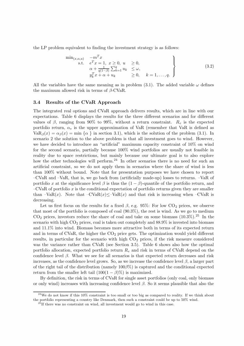
the LP problem equivalent to finding the investment strategy is as follows:

min(x,α,u) −mTx

s.t. eT x = 1, x ≥ 0, u ≥ 0,α + 1

q(1−β)

∑qk=1 uk ≤ ω,

yTk x + α + uk ≥ 0, k = 1, . . . , q.

(3.2)

All the variables have the same meaning as in problem (3.1). The added variable ω definesthe maximum allowed risk in terms of β-CVaR.

3.4 Results of the CVaR Approach

The integrated real options and CVaR approach delivers results, which are in line with ourexpectations. Table 6 displays the results for the three different scenarios and for differentvalues of β, ranging from 90% to 99%, without a return constraint. Re is the expectedportfolio return, α∗ is the upper approximation of VaR (remember that VaR is defined asVaRβ(x) = αβ(x) = min {α } in section 3.1), which is the solution of the problem (3.1). Inscenario 2 the solution to the above problem is that all investment goes to wind. However,we have decided to introduce an “artificial” maximum capacity constraint of 10% on windfor the second scenario, partially because 100% wind portfolios are usually not feasible inreality due to space restrictions, but mainly because our ultimate goal is to also explorehow the other technologies will perform.24 In other scenarios there is no need for such anartificial constraint, so we do not apply them in scenarios where the share of wind is lessthan 100% without bound. Note that for presentation purposes we have chosen to report–CVaR and –VaR, that is, we go back from (artificially made-up) losses to returns. –VaR ofportfolio x at the significance level β is thus the (1 − β)-quantile of the portfolio return, and–CVaR of portfolio x is the conditional expectation of portfolio returns given they are smallerthan –VaR(x). Note that –CVaR(x)≤–VaR(x) and that risk is increasing when –CVaR isdecreasing.

Let us first focus on the results for a fixed β, e.g. 95%: For low CO2 prices, we observethat most of the portfolio is composed of coal (90.3%), the rest is wind. As we go to mediumCO2 prices, investors reduce the share of coal and take on some biomass (10.3%).25 In thescenario with high CO2 prices, coal is taken out completely and 88.9% is invested into biomassand 11.1% into wind. Biomass becomes more attractive both in terms of its expected returnand in terms of CVaR, the higher the CO2 price gets. The optimization would yield differentresults, in particular for the scenario with high CO2 prices, if the risk measure consideredwas the variance rather than CVaR (see Section 3.5). Table 6 shows also how the optimalportfolio allocation, expected portfolio return Re and risk in terms of CVaR depend on theconfidence level β. What we see for all scenarios is that expected return decreases and riskincreases, as the confidence level grows. So, as we increase the confidence level β, a larger partof the right tail of the distribution (namely 100β%) is captured and the conditional expectedreturn from the smaller left tail (100(1 − β)%) is maximized.

By definition, the risk in terms of CVaR for single asset portfolios (only coal, only biomassor only wind) increases with increasing confidence level β. So it seems plausible that also the

24We do not know if this 10% constraint is too small or too big as compared to reality. If we think aboutthe portfolio representing a country like Denmark, then such a constraint could be up to 50% wind.

25If there was no constraint on wind, all investment would go to wind in this case.

19

β = 90% β = 95% β = 97% β = 99%

Scenario 1


Re 1.861 1.856 1.854 1.848–VaRβ 1.765 1.742 1.727 1.702–CVaRβ 1.736 1.718 1.706 1.683

Scenario 2


Re 1.712 1.710 1.708 1.706–VaRβ 1.680 1.671 1.666 1.655–CVaRβ 1.669 1.662 1.657 1.648

Scenario 3


Re 1.792 1.791 1.791 1.790–VaRβ 1.763 1.755 1.750 1.739–CVaRβ 1.753 1.746 1.741 1.733

Table 6: Optimal Portfolio Shares (in %) for Coal, Biomass and Wind, Expected Returns Re,and Risks (CVaR and VaR) for Increasing Confidence Level β and a 10% Capacity Constrainton Wind in Scenario 2 (Scenario 1: high CO2 prices; scenario 2: medium CO2 prices; scenario3: low CO2 prices. There is no constraint on the minimum level of expected return.)

optimal portfolio risk increases with growing β, which is exactly what we see in our results.Note that scenario 1 shows a growing share of wind for an increasing confidence level β.This is probably due to the fact that, for growing values of β, risk for wind is increasing lesssubstantially than that for biomass.26

Intuitively, increasing the confidence level and thus decreasing the incidence of risk, therisk in terms of expected losses in the unfavorable case (CVaR) increases. The latter is quitenatural, since the confidence level β and CVaR may be deemed as two different aspects ofrisk: β is dealing with the most probable return threshold, and CVaR deals with the returnexpectation in the unfavorable case. Obviously, one cannot reduce both the β and the CVaRsimultaneously, but a reasonable balance between those two aspects needs to be found.

Another factor that influences the optimal asset allocation is the specified level of theleast expected return, R. In Table 7, we compare the optimization results across scenariosfor increasing R, where the return constraints are chosen in the following way: The higherR is the value close to the maximum feasible value; the lower R is the minimum expectedreturn among the technologies for a given scenario; and the medium R is an arbitrarily picked

26In fact, the difference between –CVaRβ of biomass and wind is 0.0147, 0.0122, 0.0110, 0.0085 for β equalto 0.9, 0.95, 0.97, 0.99; so wind gets closer to the lowest-risk biomass with increasing confidence level.

20

value in between the higher and the lower R. In the scenario 1, we observe that the share ofbiomass increases slightly with rising R. Furthermore, Table 7 shows clearly that the valuesof CVaR do not change substantially for R=1.858 and R=1.861 in scenario 1. This meansthat for high CO2 prices the portfolio risk is quite insensitive to increases in R. This is dueto the fact that biomass and wind display rather similar degrees of risk, while the expectedreturn of biomass is higher than that of wind (see Table 3); hence the shift towards biomasswith increasing required returns.27

Scenario 1 R = 1.658 R = 1.858 R = 1.861


Re 1.856 1.858 1.861–VaR0.95 1.742 1.743 1.743–CVaR0.95 1.718 1.717 1.717

Scenario 2 R = 1.692 R = 1.720 R = 1.748


Re 1.710 1.720 1.748–VaR0.95 1.671 1.671 1.660–CVaR0.95 1.662 1.659 1.641

Scenario 3 R = 1.668 R = 1.80 R = 1.81


Re 1.791 1.80 1.81–VaR0.95 1.755 1.749 1.734–CVaR0.95 1.746 1.736 1.716

Table 7: Optimal Portfolio Shares (in %), Expected Returns Re and Risks (CVaR and VaR)for Increasing Levels of Minimum Expected Return R and a 10% Capacity Constraint onWind in Scenario 2

In scenario 2 there is a clear shift from a coal-dominated to a biomass-dominated portfoliowith an increasing minimal required return R. Note, however, the upper bound on windallocations – otherwise the optimal portfolio would be completely wind-dominated. The shiftfrom coal to biomass is due to the specific risk levels and expected returns shown by the tworespective technologies (see Table 3). The coal-fired power plant displays only a slightly lowerdegree of risk but a clearly lower expected return than biomass. The portfolio re-balancingwith increasing R, as stated above, can be easily understood then: while with a comparativelylow R the major portfolio allocation is in the lowest-risk technology feasible, which is coal(wind is constrained), the allocation shifts toward biomass, which displays only slightly higher

27Note that taking the variance as a risk measure would yield completely different optimization results,which is due to the different risk levels in terms of CVaR and variance displayed by the different technologies(see Section 3.5).

21

risk but clearly larger return, with increasing R.In scenario 3 (without the bound on wind) the optimal portfolio is re-balanced from

being coal-dominated to being wind-dominated, which can again be explained by the riskand expected return numbers of the three underlying technologies. First, biomass is notinteresting, since it displays the highest risk and lowest expected return. Coal shows a lowerrisk than wind, but also a lower return. So it is not surprising that with increasing requiredreturns R the optimal portfolio allocation shifts from the less risky coal to the slightly morerisky but also more profitable wind technology.

Scenario 1 −φ = 1.7174 −φ = 1.71745 −φ = 1.7175


Re 1.860 1.859 1.856–VaR 1.743 1.743 1.742

Scenario 2 −φ = 1.645 −φ = 1.650 −φ = 1.660


Re 1.743 1.735 1.717–VaR 1.663 1.666 1.671

Scenario 3 −φ = 1.716 −φ = 1.736 −φ = 1.745


Re 1.810 1.800 1.793–VaR 1.735 1.749 1.755

Table 8: Portfolio Shares (in %), Expected Returns Re, and Risk V aR for Decreasing Levelsof Risk in Terms of Maximum –CVaR, −φ, and Confidence Level β = 95% (All the CVaRconstraints are active, i.e. the actual value of –CVaR is equal to the constraint value −φ.)

In general, the degree and direction of portfolio re-balancing with increasing minimalreturns depend on the risk and return structure of the underlying assets. In particular,it depends on the difference between risk and expected return levels of the assets. In oursituation, biomass has the highest expected return and, at the same time, the lowest degreeof risk in scenario 1; the same is true for wind in scenario 2. This explains why a major partof the optimal portfolio in the first scenario is invested into biomass; in the scenario 2, thesituation is different due to the upper bound on wind allocations. In the third scenario, coaldisplays the lowest risk, while the highest expected return is gained by investing in wind,which explains the portfolio re-balancing from a coal-dominated allocation to a portfolio,where wind is prevalent. In addition, coal displays the highest risk and lowest expectedreturn in the first scenario and hence is clearly dominated by the other two technologies. Thesame applies to biomass in the third scenario. This is why optimal portfolios do never includecoal in the first scenario and biomass in the third scenario.

Table 8 shows the investment strategies and corresponding expected returns under a CVaR

22

risk constraint. Scenario 1 is quite insensitive to and therefore stable across different CVaRrestrictions, so both expected return and risk α∗ change only slightly, when the CVaR restric-tion changes. In other scenarios, this insensitivity only holds up to a certain level, beyondwhich the portfolios change substantially: While there is no outstanding technology changein the portfolio composition in scenario 1, in scenarios 2 and 3 coal replaces biomass and windrespectively, as the maximum allowed risk decreases. Furthermore, Table 8 shows a slightincrease in risk α∗ for the lower admissible level of CVaR-risk φ for scenario 1. Please notethat this is not contradictory, since section 3.2 explained that α∗ is the threshold of the lossfunction, which is the upper approximation of β-VaR and not necessarily the exact value ofβ-VaR according to its definition in section 3.1.

3.5 Mean-variance versus CVaR

In spite of its failures in the case of non-normal or non-symmetric distributions the mean-variance (M-V) approach posed by Markowitz, see Markowitz (1959), still enjoys widespreadacceptance as a practical tool for portfolio construction, and many investment firms routinelycompute mean-variance efficient portfolios. Rockafellar and Uryasev (2000) have shown thatunder certain conditions the CVaR approach and the M-V approach are equivalent in termsof providing the same optimal asset allocations. Thus, the CVaR approach can be viewed insome sense as a generalization of the M-V approach when dealing with non-normal or non-symmetric distributions. From this perspective it makes sense to consider the M-V approachas a benchmark case and thus to compare its performance to that of CVaR.

The M-V optimization problem under consideration is formulated as follows

min{

xT Cx | x ≥ 0, mT x ≥ R, eT x = 1}

(3.3)

where C is the covariance matrix of the return distribution of instruments under consideration,x ∈ R

n is the vector of portfolio holdings, m ∈ Rn is the vector of expected returns, e ∈ R

n

is the vector of ones and parameter R ∈ R is the minimum expected return. Under thejoint normality assumption of returns, the portfolio distribution, which is normal, is uniquelydefined by its first two moments (mean and variance). In the M-V framework, risk is defined asthe variance of the portfolio return, xT Cx, and thus the task is to minimize portfolio variancewith respect to a certain aversion towards risk, which is represented by the minimum expectedreturn R the portfolio needs to achieve. Note that for a small number of instruments (in ourcase n = 3), the quadratic programming (QP) problem (3.3) will be solved much faster thanthe linear programming problem for solving CVaR.28

Table 9 and Figure 5 present comparisons of different performance measures computedfor the M-V and CVaR portfolios for different minimum values of expected returns, R, asreported in Table 7. As an additional reference case we have calculated M-V portfolios underthe assumption of uncorrelated returns of our power plants.29

As performance measures we use expected return, variance, –CVaR and –VaR. Preferredoutputs are larger values of expected returns, –CVaR, –VaR; and smaller values of variances.

28The LP problem for finding the portfolio with minimum CVaR has q +n+1 = 10, 004 variables while theQP problem for finding the M-V portfolio has only n = 3 variables.

29There is a closed form solution for solving the parametric quadratic programming problems under theassumption that the covariance matrix is diagonal, and for a certain range of parameter R the portfolio willbe diversified by construction (see Best and Hlouskova, 2000).

23

In scenario 1 (high CO2 prices), CVaR portfolios show a performance which is clearlysuperior to that of M-V portfolios for R ∈ {1.658, 1.75}, see the density plots of both portfoliosat the first line in Figure 5 where the majority of the mass of CVaR portfolios is to the rightof the mass of M-V portfolios. For both values of R under consideration (R = 1.658, whichis the return of the coal-fired power plant, and R = 1.75), CVaR portfolios outperform M-Vportfolios when the portfolio performance is measured by expected return, CVaR and VaR.The return of the M-V portfolio has smaller variance than the one of the CVaR portfolio.Interestingly, the M-V portfolio with assumed uncorrelated power plants’ returns shows abetter performance with respect to all measures (but variance) than the M-V portfolio withthe true covariance matrix. Portfolio holdings between CVaR and M-V portfolios differ quitedramatically: while the CVaR approach poses most weight to the biomass-fired power plant,the M-V approach places most weight to the coal-fired power plant (when R = 1.658) and tothe coal-fired power plant and the wind mill (when R = 1.75). For R ∈ {1.858, 1.861} theM-V and CVaR portfolios coincide.

The differences in the portfolio performance between M-V and CVaR are significantlysmaller in scenario 2 (medium CO2 prices). The deterioration of the performance of theCVaR portfolio compared to the unconstrained M-V portfolio for bigger R comes from theimposition of 10% upper bound on wind-mill holdings (otherwise CVaR portfolio consistsonly of the wind-mill). For R = 1.692 the CVaR portfolio still performs best (except forthe variance). However, when comparing it with the M-V portfolio with zero correlationsthen all the performance measures as well as portfolio holdings are in the same ballpark. Forhigher values of the expected return, R ∈ {1.72, 1.748}, the M-V portfolio where the 10%bound on wind-mill holdings was not imposed outperforms the constrained CVaR portfolioin all measures but expected return which is the same. Note that when the 10% bound onwind-mill holdings was imposed also in the M-V problem, then the CVaR and M-V portfolioscoincide.

The CVaR portfolio seems to perform best in scenario 3 (low CO2 prices) only in the casewhen R = 1.688 for all measures but variance. For R = 1.791, which is far from its maximumvalue (see Table 6 on expected returns of power plants), the CVaR and M-V portfolios aremore or less the same (the density plots are nearly identical). The next empirical observationfollows also from Proposition 1 in Rockafellar and Uryasev (2000), which says that undercertain assumptions CVaR and M-V portfolios coincide. These assumptions are: the returnassociated with each portfolio is normally distributed, β ≥ 0.5 and the constraint on expectedreturn is active. We have performed a normality test on the M-V and CVaR portfolios forR = 1.791 in scenario 3, and the null hypothesis on normality was not rejected at the 10%significance level.30 Note that expected returns of both portfolios coincide with R = 1.791.;i.e. the return constraint is active. Thus, observing identical density plots does not come asa surprise. On the other hand, M-V and CVaR portfolios coincide for R ∈ {1.8, 1.81}, theirconstraints on expected returns are active, and their return distribution is non-normal.31

Thus, the main observation is that the performance differences between CVaR and M-Vportfolios are largest for scenario 1 (high CO2 prices). One cannot see such pronounced dif-ferences in performance measures in scenarios 2 and 3, where CO2 prices are equal to the

30This could be the consequence of the fact that normality was not rejected at the 10% significance levelfor the return distribution of the coal-fired power plant, and the biggest weight (app. 90%) was allocated tothis power plant.

31In these cases most of the weight is allocated to the biomass-fired power plant where the null hypothesisof the return distribution being normal was rejected at the 1% significance level.

24

mean and low respectively. The same concerns portfolio holdings. This observation opposesthe observation made in Krokhmal, Palmquist and Uryasev (2001), where no significant dif-ferences between CVaR and M-V portfolios were noticed. However, as the authors mention,their result is dataset-specific – and so is ours. The significant differences between the per-formance of CVaR and VaR portfolios and the massive outperformance of CVaR portfoliosin scenario 1 have to be associated with the fact that individual plant returns and portfolioreturns are non-normal. A normality test for the M-V portfolio returns showed that the nullhypothesis of normality can be rejected.32 We find our exercise a helpful demonstration ofadvantages of the CVaR approach over the M-V approach. We have also empirically con-firmed that the M-V approach is embedded in the CVaR framework (by simple applicationof the findings of Rockafellar and Uryasev (2000)). Thus, being cautious when choosing theportfolio optimization approach seems to be a wise idea.

1.5 1.6 1.7 1.8 1.9 2 2.10

5

10

15

20

1.5 1.6 1.7 1.8 1.9 2 2.10

5

10

15

20

1.5 1.6 1.7 1.8 1.9 2 2.10

5

10

15

20

1.5 1.6 1.7 1.8 1.9 2 2.10

5

10

15

20

1.5 1.6 1.7 1.8 1.9 2 2.10

5

10

15

20

1.5 1.6 1.7 1.8 1.9 2 2.10

5

10

15

20

1.5 1.6 1.7 1.8 1.9 2 2.10

5

10

15

20

1.5 1.6 1.7 1.8 1.9 2 2.10

5

10

15

20

1.5 1.6 1.7 1.8 1.9 2 2.10

5

10

15

20

Figure 5: Density Plots of Returns of CVaR and M-V Portfolios (Row 1: Scenario 1 (highCO2 prices). Row 2: Scenario 2 (medium CO2 prices). Row 3: Scenario 3 (low CO2 prices).The black solid line corresponds to CVaR, the dashed line to M-V and the dotted line toM-V portfolios (no correlation assumption). Figure 1 in the row 1 has R = 1.658, Figure 2has R = 1.75, and Figure 3 has R = 1.858. In row 2 R is chosen as follows (left to right):R = 1.692, 1.7202, 1.7484. The upper bound is imposed in scenario 2 for the CVaR model:x3 ≤ 0.1 (x3 corresponds to holdings of wind). In row 3 R is chosen as follows (left to right):R = 1.668, 1.8, 1.81. β = 95% for CVaR portfolios).

32All normality tests were conducted by applying the Jarque-Bera test.

25

Scenario R Additional constraint Opt. type Coal Biomass Wind Re Variance (%) -CVaR -VaR

1 1.658 - M-V 100.0 0.0 0.0 1.658 0.034 1.621 1.6281 1.658 uncorrelated returns M-V 85.5 4.8 9.7 1.683 0.049 1.639 1.6481 1.658 - CVaR 0.0 88.9 11.1 1.856 0.560 1.718 1.742

1 1.750 - M-V 45.3 13.7 41.0 1.750 0.140 1.675 1.6901 1.750 - CVaR 0.0 88.9 11.1 1.856 0.560 1.718 1.742

1 1.858 - M-V, CVaR 0.0 93.4 6.6 1.858 0.582 1.717 1.743

1 1.861 - M-V, CVaR 0.0 99.8 0.2 1.861 0.614 1.717 1.743

2 1.692 - M-V 100.0 0.0 0.0 1.692 0.037 1.654 1.6612 1.692 uncorrelated returns M-V 81.4 8.6 10.0 1.709 0.056 1.661 1.6712 1.692 x3 ≤ 0.1 CVaR 79.7 10.3 10.0 1.709 0.060 1.662 1.671

2 1.720 - M-V 77.2 0.0 22.8 1.720 0.070 1.668 1.6792 1.720 x3 ≤ 0.1 M-V, CVaR 57.9 32.1 10.0 1.720 0.100 1.659 1.671

2 1.748 - M-V 54.1 0.0 45.9 1.748 0.115 1.681 1.6952 1.748 x3 ≤ 0.1 M-V, CVaR 0.2 89.8 10.0 1.748 0.337 1.641 1.660

3 1.668 - M-V 83.9 16.1 0.0 1.769 0.043 1.727 1.7353 1.668 uncorrelated returns M-V 61.6 29.1 9.3 1.756 0.055 1.708 1.7183 1.668 - CVaR 90.3 0.0 9.7 1.791 0.049 1.746 1.755

3 1.791 - M-V 91.2 0.0 8.8 1.791 0.049 1.746 1.7553 1.791 - CVaR 90.3 0.0 9.7 1.791 0.052 1.746 1.755

3 1.800 - M-V, CVaR 55.7 0.0 44.3 1.800 0.073 1.736 1.749

3 1.810 - M-V, CVaR 17.6 0.0 82.4 1.810 0.205 1.716 1.734

Table 9: Portfolio Allocations (in %) and Performance for M-V and CVaR Portfolios Scenario 1 represents high CO2 prices, scenario2 represents medium CO2 prices and scenario 3 represents low CO2 prices. Re is the expected return, β = 95%, and x3 correspondsto the holdings of the wind farm.

26

4 Conclusion

Energy investments have raised the interest of many large investors recently. The enactmentof climate change policies aiming to reduce CO2 emissions by punishing fossil fuel technologiesthrough taxes and the establishment of permit trading schemes have made investments in theelectricity sector different from what they were before: More environmentally friendly tech-nologies, which had previously been largely unprofitable due to high capital and operations& maintenance cost and low load factors (e.g. wind energy suffers from the fact that winddoes not always blow at constant speed), have become much more attractive in the light ofthese new climate change policies.

It has been shown in several studies (e.g. Fuss et al, 2006; Laurikka and Koljonen,2006) that the uncertainties originating in the CO2 price and the electricity price, whichthe individual power plant investor faces, can be incorporated in the investment decision byusing real options modeling. However, if we think of larger power plant investors or banksproviding funds to those investors, it seems to be natural that they would like to diversifyinvestments. A bank, for example, will provide funds not only to power plants with highexpected returns, since these usually come at the cost of higher risk, but also to power plantswith lower expected returns, if they can demonstrate on solid grounds that they are exposedto a lower degree of risk.

While these diversification ideas are generally familiar through the work of Nobel laureateMarkowitz (1952), they have – so far – not been extensively applied to investment planningin the electricity sector. We have therefore developed a portfolio optimization approachwhich uses the return distributions resulting from a decision-making process of the powerplant producer within a real options framework. As a measure of risk we have chosen CVaRbecause we think it is more appropriate for our problem than the traditional mean-varianceapproach for a multitude of advantages listed in previous sections. Under mild assumptions,Value-at-Risk minimization, conditional Value-at-Risk minimization and the mean-varianceapproach all yield the same results, provided that all underlying distributions are normal.We have seen, however, that the (bivariate) dependence structure between different returnsfails to be normal. Results from estimating a restricted symmetric version of a fairly flexiblecopula showed that in nearly all cases (coal/biomass, coal/wind and biomass/wind in thethree scenarios) the null hypothesis of symmetry could be rejected. This seems to be clearevidence of non-normality in the total joint return distribution and thus implies that it is moresensible to use the CVaR approach in portfolio optimization than the mean-variance (M-V)approach where the return distribution is supposed to be normally distributed. Our empiricalresults in terms of comparisons of different performance measures of the CVaR and the M-Vportfolios as well as the density plots of return distributions of these portfolios (mainly forthe scenario with high CO2 prices) are clear consequences of this evidence.

Our results show that the combined RO-CVaR approach is indeed a valuable contributionto the existing theory on investment under uncertainty in the electricity sector. More specifi-cally, we find that the results are in line with what we would expect in terms of diversification:As we increase the level of β the investor starts to favor low-risk over high-risk technologies,even if expected returns are lower. With respect to the minimum expected return R that theinvestor specifies, the portfolios shift to technologies with higher expected returns as R in-creases. So, the extent of the risk looses importance in the investment decision if the expectedreturn that the investor wants to secure gets higher.

From a policy perspective, we can say that already for low CO2 prices, the mere fact that

27

the investor wants to diversify to reduce the risk for a given return leads to the inclusionof renewables (here wind) into the portfolio because with increasing CO2 prices, wind isrelatively more profitable than investors might initially have assumed. Fossil fuel technologies(here coal), on the other hand have more stable returns, so they make up the larger part ofthe portfolio in the case of low CO2 prices. For coal, expected returns fall, as we go from thethird to the first scenario. In the first scenario biomass has an expected return even largerthan wind, but the fact that biomass and wind display similar degrees of risk leads to theinclusion of both technologies in the optimal portfolio. Finally, in the first scenario, fossil fuels(coal) do no longer play a major role, which is exactly what policymakers want to achieve byraising the price of CO2 more sharply.

28

Appendix A: Snapshots of Price Distributions for All Scenarios

Figure A.1: Price Distributions of CO2 in Scenarios 1, 2, 3 and of Electricity (The graphpresents bar charts of CO2 prices for scenarios 1, 2 and 3, and of electricity prices (top tobottom) for years 10, 30 and 50 (left to right). The horizontal axis shows prices in e , thevertical axis shows frequencies in %.)

29

Appendix B: Real Options Output for Investing and Switching

Figure B.1: Investment Frequencies for Adding CCS to Coal (left) and Biomass (right) forThree Scenarios (high CO2 prices (top row), normal CO2 prices (middle row), low CO2 prices(bottom row) for 10,000 simulations)

30

Figure B.2: Frequencies of Switching the CCS Module Off for Coal (left) and Biomass(right)(high CO2 prices (top row), normal CO2 prices (middle row), low CO2 prices (bot-tom row) for 10,000 simulations)

31

Figure B.3: Frequencies of Switching the CCS Module On for Coal (left) and Biomass (right)(high CO2 prices (top row), normal CO2 prices (middle row), low CO2 prices (bottom row)for 10,000 simulations)

32

Appendix C: Definitions of Copulas and Related Concepts

A copula is a function C : I2 = [0, 1]2 → I, satisfying, for 0 ≤ u ≤ 1 and u1 ≤ u2, v1 ≤v2, (u1, u2), (v1, v2) ∈ I2, the conditions

C(u, 0) = C(0, u) = 0, C(u, 1) = C(1, u) = u, (C.1)

C(u2, v2) − C(u1, v2) − C(u2, v1) + C(u1, v1) ≥ 0. (C.2)

The second condition means that P (u1 ≤ U ≤ u2, v1 ≤ V ≤ v2) ≥ 0 for (U, V ) having jointdistribution function C. See Nelsen (2006) for further details.

To better understand the concept of a copula consider Sklar’s theorem. Let F be thedistribution function of random variables (X, Y ) with marginal distribution functions F1 andF2. Then there exists a copula C : I2 → I such that, for all (X,Y ),

F (X,Y ) = C(F1(X), F2(Y )). (C.3)

If F1 and F2 are continuous, then C is unique. Otherwise, C is uniquely determined onRanF1 × RanF2. The copula can be computed as C(U, V ) = F (F −1

1 (X), F−12 (Y )). Con-

versely, if C is a copula and F1 and F2 are one-dimensional distribution functions, then thefunction F defined by (C.3) is a two-dimensional distribution function with margins F1, F2.Clearly, a copula itself is a distribution function. Note that random variables transformed bytheir marginal probability distribution functions, i.e. F1(X) and F2(Y ), are standard uniformrandom variables (U , V ).

Let C be a copula. Then lower tail dependence and upper tail dependence are defined as

λL = limα→0+

P (U ≤ α|V ≤ α) = limα→0+

C(α, α)

α,

λU = limα→0+

P (U > 1 − α|V > 1 − α) = limα→0+

2α − 1 + C(1 − α, 1 − α)

α,

provided the limit exists. Note that 0 ≤ λL, λU ≤ 1. Using Sklar’s theorem, lower and uppertail dependence can also be understood in terms of random variables X and Y with marginaldistribution functions F1 and F2, viz

λL = limα→0+

P [X ≤ F−11 (α)|Y ≤ F−1

2 (α)],

λU = limα→0+

P [X > F−11 (1 − α)|Y > F−1

2 (1 − α)].

Another function of the copula describing dependence is Kendall’s tau. While the com-monly used linear correlation is not only a function of the copula but depends also on themarginal distributions, the rank correlation Kendall’s tau τ , where −1 ≤ τ ≤ 1, can beexpressed in terms of the copula only,

τ(U, V ) = 4

∫ 1

0

∫ 1

0C(U, V )dC − 1 = 4E(C(U, V )) − 1.

The two-parametric BB1 copula, which is used in this application, takes the followingfunctional form,

C(u, v) = {1 + [(u−θ − 1)δ + (v−θ − 1)δ ]1/δ}−1/θ,

33

where θ > 0 and δ ≥ 1, see Joe (1997) for details. The BB1 copula nests two widely usedone-parametric Archimedean copulas, the Gumbel and the Clayton. The Gumbel is the limitof the BB1 for θ → 0, the Clayton arises when δ = 1. The BB1 can display positive anddifferent lower and upper tail dependence and has a closed form for Kendall’s tau. Lower andupper tail dependence, and Kendall’s tau for the BB1 copula are

λL = 2−1/(θδ),

λU = 2 − 21/δ ,

τ = 1 −2

δ(θ + 2).

The estimation procedure employs maximum likelihood. Since we do not want to imposespecific forms of the univariate marginal distributions, we use empirical marginal distributionfunctions. For statistical properties of the resulting estimators see Genest and Rivest (1993)and Genest et al (1995). For an application of copulas in international stock markets, see forexample Fortin and Kuzmics (2002).

34

References

Alesii, G. (2005): “VaR in Real Options Analysis,” Review of Financial Economics, 14,189–208.

Annaert, J., G. Deelstra, D. Heyman, and M. Vanmaele (2006): “Risk Managamentof a Bond Portfolio Using Options,” Mathematics and Economics, in press.

Artzner, P., F. Delbaen, J. Eber, and D. Heath (1997): “Thinking Coherently,” Risk,10, 68–71.

Best, M., and J. Hlouskova (2000): “The efficient frontier for bounded assets,” Mathe-matical Methods of Operations Research, 52, 195–212.

Bogentoft, E., H. Romeijn, and S. Uryasev (2001): “Asset/Liability Management forPension Funds Using CVaR Constraints,” Journal of Risk, pp. 57–71.

Chladna, Z., M. Chladny, K. Mollersten, and M. Obersteiner (2004): “Investmentunder Multiple Uncertainties,” Interim Report IR-04-077, International Institute of AppliedSystems Analysis.

de Jong, C., A. Oosterom, and K. Walet (2004): “Dealing with Emissions,” in Man-aging Energy Price Risk - The New Challenges and Solutions, ed. by V. Kaminski, RiskBooks. Barclay, Division of Incisive Financial Planning Ltd., 3 edn.

Dixit, A., and R. Pindyck (1994): Investment under Uncertainty. Princeton UniversityPress, Princeton.

Doege, J., P. Schiltknecht, and H.-J. Luthi (2006): “Risk Management of PowerPortfolios and Valuation of Flexibility,” OR Spectrum, 28, 267–287.

Farzin, Y., K. Huisman, and P. Kort (1998): “Optimal Timing of Technology Adoption,”Journal of Economic Dynamics and Control, 22, 779–799.

Fichtner, W., M. Gobelt, and O. Rentz (2002): “Ein Modell zur strategischenInvestitions- und Produktionsplanung bei Energieversorgern unter Berucksichtung von Un-sicherheiten,” ZfE - Zeitschrift fur Energiewirtschaft, 26(3), 181–192.

Fleten, S., K. Maribu, and I. Wangensteen (2006): “Optimal Investment Strategies inDecentralized Renewable Power Generation under Uncertainty,” Energy, in press(correctedproof).

Fortin, I., and C. Kuzmics (2002): “Tail-Dependence in Stock-Return Pairs,” InternationalJournal of Intelligent Systems in Accounting, Finance & Management, 11, 89–107.

Fuss, S., J. Szolgayova, M. Gusti, and M. Obersteiner (2006a): “The Effects ofLearning on Investment under Market and Climate Policy Uncertainty,” Working paper,International Institute of Applied Systems Analysis.

(2006b): “Investment Response to Uncertainty in Regulation in the ElectricitySector,” Interim Report IR-06-xxx, International Institute of Applied Systems Analysis.

35

Genest, C., K. Ghoudi, and L.-P. Rivest (1995): “A Semiparametric Estimation Pro-cedure of Dependence Parameters in Multivariate Families of Distributions,” Biometrica,82, 7543–552.

Genest, C., and L.-P. Rivest (1993): “Statistical Inference Procedures for BivariateArchimedean Copulas,” Journal of American Statistical Association, 88, 1034–1043.

Hlouskova, J., S. Kossmeier, M. Obersteiner, and A. Schnabl (2005): “Real Op-tions and the Value of Generation Capacity in the German Electricity Market,” Review ofFinancial Economics, 14(3-4), 297–310.

International Energy Agency (2005): Projected Costs of Generating Electricity 2005Update. OECD Nuclear Energy Agency, Paris.

Joe, H. (1997): Multivariate Models and Dependence Concepts. Chapman and Hall, London.

Kiriyama, E., and A. Suzuki (2004): “Use of Real Options in Nuclear Power Plant Valua-tion in the Presence of Uncertainty with CO2 Emission Credit,” Journal of Nuclear Scienceand Technology, 41(7), 756–764.

Krokhmal, P., J. Palmquist, and S. Uryasev (2001): “Portfolio Optimization withConditional Value-at-Risk Objective and Constraints,” Journal of Risk, 4, 43–68.

Krokhmal, P., S. Uryasev, and G. Zrazhevsky (2003): “Numerical Comparison ofCVaR and CDaR Approaches: Application to Hedge Funds,” Discussion paper, Risk Man-agement and Financial Engineering Lab, Department of Industrial and Systems EngineeringUniversity of Florida.

Kulatilaka, N. (1988): “Valuing the Flexibility of Flezible Manufacturing Systems,” IEEETransactions on Engineering Management, 35(4), 250–257.

Kumbaroglu, G., R. Madlener, and M. Demirel (2004): “A Real Options EvaluationModel for the Diffusion Prospects of New Renewable Power Generation Technologies,”Working paper no. 35, Centre for Energy Policy and Economics Working Papers.

Laurikka, H. (2004): “The Impact of Climate Policy on Heat and Power Capacity Invest-ment Decisions,” in Proceedings of the Workshop ”Business and Emissions Trading”, ed.by B. Hansjurgens. forthcoming, Wittenberg, Germany.

Laurikka, H., and T. Koljonen (2006): “Emissions Trading and Investment Decisions inthe Power Sector - a Case Study of Finland,” Energy Policy, 34, 1063–1074.

Liu, J., C. Men, V. Cabrera, S. Uryasev, and C. Fraisse (2006): “CVaR Model forOptimizing Crop Insurance under Climate Variability,” Discussion paper, Risk Manage-ment and Financial Engineering Lab, Department of Industrial and Systems EngineeringUniversity of Florida.

Madlener, R., and W. Gao (2005): “Renewable Energy Policy in the Presence of Innova-tion: Does Pre-commitment by the Government Matter?,” Working paper no. 46, Centrefor Energy Policy and Economics Working Papers.

Markowitz, H. (1952): “Portfolio Selection,” Journal of Finance, 7(1), 77–91.

36

(1959): Portfolio Selection: Efficient Diversification of Investments. Wiley.

McDonald, R., and D. Siegel (1986): “The Value of Waiting to Invest,” Quarterly Journalof Economics, 101, 707–723.

Merton, R. (1973): “The Theory of Rational Option Pricing,” Journal of Economic Man-agement Science, 4, 141–183.

Messner, S., and M. Strubegger (1995): “User’s Guide for MESSAGE III,” Wp 95-69,International Institute for Applied Systems Analysis.

Murto, P. (2006): “Timing of Investment under Technological and Revenue-Related Uncer-tainties,” Journal of Economic Dynamics and Control, in press.

Nelsen, R. (2006): An Introduction to Copulas. Springer, Berlin, 2nd edn.

on Banking Supervision, B. C. (2003): “Trends in Risk Integration and Aggregation,”Discussion paper, Bank for International Settlements.

(2006): “International Convergence of Capital Measurement and Capital Standards,”Discussion paper, Bank for International Settlements.

Palmquist, J., S. Uryasev, and P. Krokhmal (2002): “Portfolio Optimization withConditional Value-at-Risk Objective and Constraints,” The Journal of Risk, 4(2).

Pindyck, R. (1988): “Irreversible Investment, Capacity Choice, and the Value of the Firm,”American Economic Review, 79, 969–985.

(1991): “Irreversibility, Uncertainty and Investment,” Journal of Economic Litera-ture, 29, 1110–1152.

(1993): “Investments of Uncertain Cost,” Journal of Financial Economics, 34, 53–76.

Reedman, L., P. Graham, and P. Coombes (2006): “Using a Real Options Approachto Model Technology Adoption Under Carbon Price Uncertainty: An Application to theAustralian Electricity Generation Sector,” The Economic Record, 82(special issue), 64–73.

Riahi, K., A. Grubler, and N. Nakicenovic (2006): “Scenarios of Long-term Socio-economic and Environmental Development under Climate Stabilization,” TechnologicalForecasting and Social Change, article in press(special issue).

Rockafellar, R., and S. Uryasev (2000): “Optimization of Coditional Value at Risk,”Journal of Risk, 2, 21–42.

(2002): “Conditional Value at Risk for General Loss Distributions,” Journal ofBanking and Finance, 26, 1443–1471.

Schnitkey, G., B. Sherrick, and S. Irwin (2004): “The Performance of ConditionalValue-at-Risk Versus Value-at-Risk in Ranking Crop Insurance Alternatives,” Discussionpaper, Department of Agricultural and Consumer Economics University of Illinois atUrbana-Champaign.

37

Schwartz, E., and L. Trigeorgis (2001): Real Options and Investment under Uncertainty:Classical Readings and Recent Contributions. The MIT Press, Cambridge/Mass.

Spangardt, G. Lucht, M., and E. Handschin (2006): “Applications for stochastic opti-mization in the power industry,” Electrical Engineering, 88, 177–182.

Stern, N. (2006): “The Economics of Climate Change,” Discussion paper, Cabinet Office -HM Treasury.

Topaloglou, N., H. Vladimirou, and S. Zenios (2003): “CVaR Models with SelectiveHedging for International Asset Allocation,” Journal of Banking and Finance, 26(7), 1535–1561.

Trigeorgis, L. (1996): Real Options: Managerial Flexibility and Strategy in Resource Allo-cation. The MIT Press, Cambridge/Mass.

Tseng, C., and G. Barz (2002): “Short-term Generation Asset Valuation: A Real OptionsApproach,” Operations Research, 50(2), 297–310.

Unger, G., and H.-J. Luthi (2002): “Power Portfolio Optimization and the Importance ofOperational Flexibility,” Discussion paper, IFOR, ETH Zentrum.

38

Authors: Ines Fortin, Sabine Fuss, Jaroslava Hlouskova, Nikolay Khabarov, Michael Obersteiner, Jana Szolgayova Title: An Integrated CVaR and Real Options Approach to Investments in the Energy Sector Reihe Ökonomie / Economics Series 209 Editor: Robert M. Kunst (Econometrics) Associate Editors: Walter Fisher (Macroeconomics), Klaus Ritzberger (Microeconomics) ISSN: 1605-7996 © 2007 by the Department of Economics and Finance, Institute for Advanced Studies (IHS), Stumpergasse 56, A-1060 Vienna • +43 1 59991-0 • Fax +43 1 59991-555 • http://www.ihs.ac.at

ISSN: 1605-7996

an integrated cvar and real options approach to ... · an integrated cvar and real options approach...

Documents