an indoor alternative to stereographic spherical...

An Indoor Alternative to Stereographic Spherical Panoramas

Chamberlain Fong

San Francisco, California USA [email protected]

Abstract The stereographic projection is a popular method for viewing spherical panoramas because of its ability to represent the scene as a “little planet” with a simulated overhead view. However, the stereographic projection does not work well for indoor scenes. In this paper, we present a method for producing a counterpart to the stereographic projection for indoor scenes. The main innovation of our method is the introduction of a novel azimuthal map projection that can smoothly blend between the stereographic projection and the Lambert azimuthal equal-area projection. Our projection has an adjustable parameter that allows one to control and compromise between distortions in shape and distortions in size within the projected panorama. This extra control parameter gives our projection the ability to produce superior results over the stereographic projection.

1. Introduction

Recent advancements in image stitching algorithms and fisheye lens optics have made capturing spherical panoramas easier than ever. Consequently, there are a growing number of photographers who work with such images. Spherical panoramas are the widest possible photographs that one can capture from a single viewpoint. They capture the entire sphere of light that shines over the photographer into a single image. However, spherical panoramas cannot be viewed easily unless projected to a planar image.

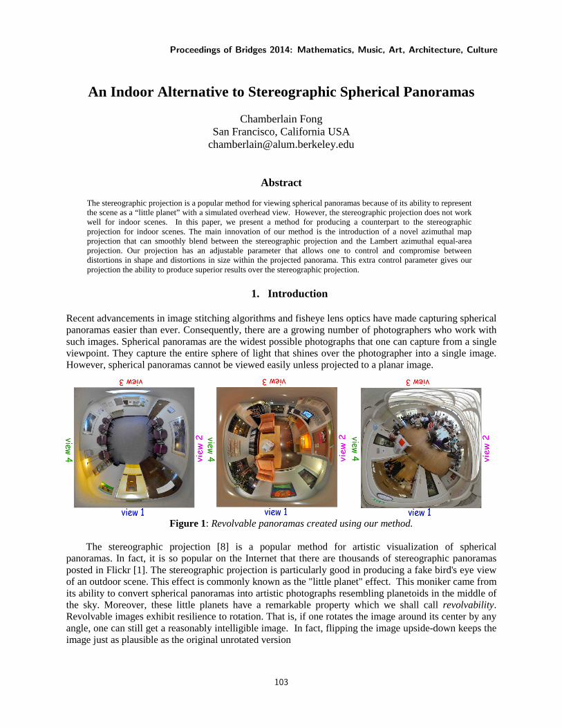
Figure 1: Revolvable panoramas created using our method.

The stereographic projection [8] is a popular method for artistic visualization of spherical panoramas. In fact, it is so popular on the Internet that there are thousands of stereographic panoramas posted in Flickr [1]. The stereographic projection is particularly good in producing a fake bird's eye view of an outdoor scene. This effect is commonly known as the "little planet" effect. This moniker came from its ability to convert spherical panoramas into artistic photographs resembling planetoids in the middle of the sky. Moreover, these little planets have a remarkable property which we shall call revolvability. Revolvable images exhibit resilience to rotation. That is, if one rotates the image around its center by any angle, one can still get a reasonably intelligible image. In fact, flipping the image upside-down keeps the image just as plausible as the original unrotated version

Proceedings of Bridges 2014: Mathematics, Music, Art, Architecture, Culture

103

In this paper, we will present a spherical map projection derived from blending the stereographic projection with the Lambert azimuthal equal-area projection. This proposed projection can also be considered as a generalization of both projections. Like the stereographic projection, our projection can be used to convert a spherical panorama into a photograph with a simulated overhead view of the scene. In addition, the resulting image will also be revolvable. Unlike the stereographic projection, our projection is suitable for indoor scenes. Figure 1 shows some examples of our results.

So, why is the stereographic projection suitable for outdoor scenes but not for indoor scenes? Usually, in outdoor scenes, the topmost region of the panorama is just the homogeneous blue sky. This region can be cropped out without adversely affecting the overall panorama. In contrast, for indoor scenes, cropping the ceiling out usually makes the panorama look incomplete. On the other hand, including too much of the ceiling causes significant size disproportions between the ceiling and the floor. See Figure 9 for a sneak peek of a picture showing the deficiencies of the stereographic projection for indoor panoramas.

2. Algorithmic Overview

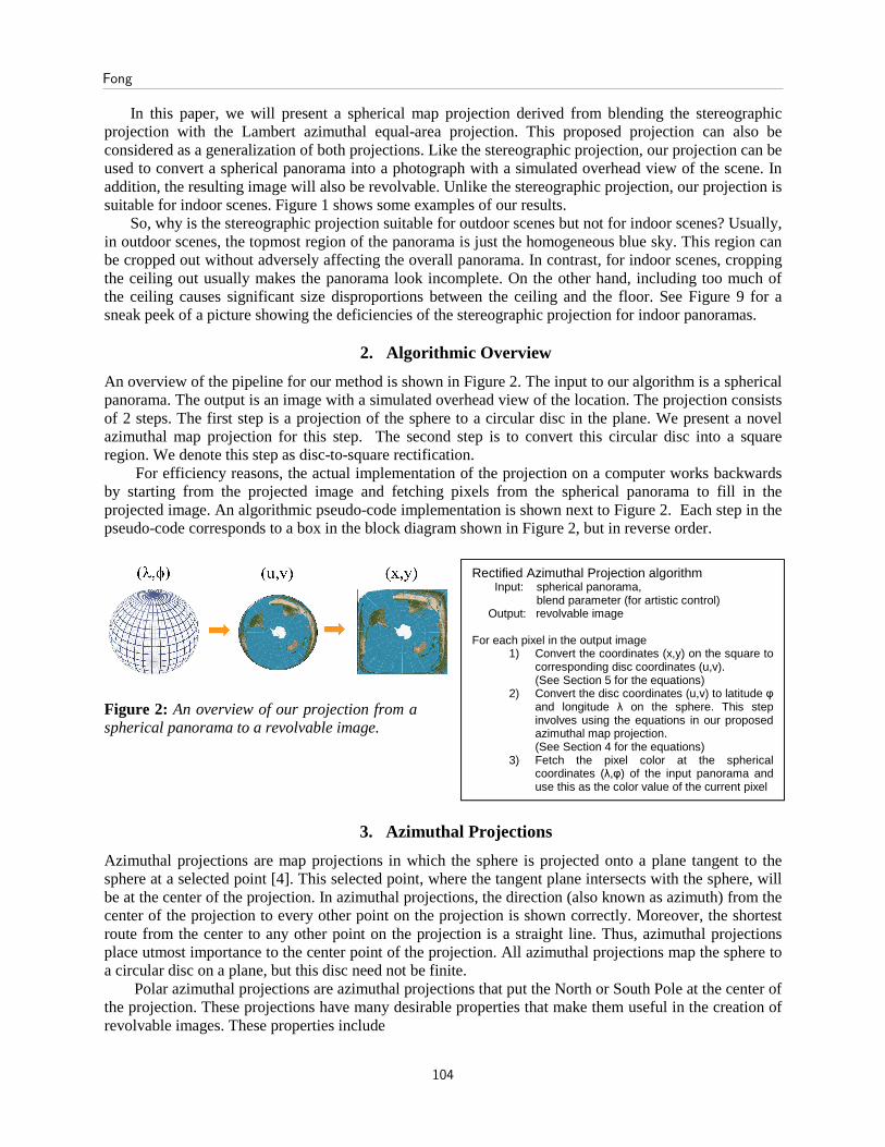
An overview of the pipeline for our method is shown in Figure 2. The input to our algorithm is a spherical panorama. The output is an image with a simulated overhead view of the location. The projection consists of 2 steps. The first step is a projection of the sphere to a circular disc in the plane. We present a novel azimuthal map projection for this step. The second step is to convert this circular disc into a square region. We denote this step as disc-to-square rectification.

For efficiency reasons, the actual implementation of the projection on a computer works backwards by starting from the projected image and fetching pixels from the spherical panorama to fill in the projected image. An algorithmic pseudo-code implementation is shown next to Figure 2. Each step in the pseudo-code corresponds to a box in the block diagram shown in Figure 2, but in reverse order.

Figure 2: An overview of our projection from a spherical panorama to a revolvable image.

3. Azimuthal Projections

Azimuthal projections are map projections in which the sphere is projected onto a plane tangent to the sphere at a selected point [4]. This selected point, where the tangent plane intersects with the sphere, will be at the center of the projection. In azimuthal projections, the direction (also known as azimuth) from the center of the projection to every other point on the projection is shown correctly. Moreover, the shortest route from the center to any other point on the projection is a straight line. Thus, azimuthal projections place utmost importance to the center point of the projection. All azimuthal projections map the sphere to a circular disc on a plane, but this disc need not be finite.

Polar azimuthal projections are azimuthal projections that put the North or South Pole at the center of the projection. These projections have many desirable properties that make them useful in the creation of revolvable images. These properties include

Rectified Azimuthal Projection algorithm Input: spherical panorama, blend parameter (for artistic control) Output: revolvable image For each pixel in the output image

1) Convert the coordinates (x,y) on the square to corresponding disc coordinates (u,v). (See Section 5 for the equations)

2) Convert the disc coordinates (u,v) to latitude φ and longitude λ on the sphere. This step involves using the equations in our proposed azimuthal map projection. (See Section 4 for the equations)

3) Fetch the pixel color at the spherical coordinates (λ,φ) of the input panorama and use this as the color value of the current pixel

Fong

104

• There is radial symmetry of scale around the center, which produces naturally circular images; • Meridians of constant longitude are straight lines emanating radially from the center; • Parallels of constant latitude are concentric circles centered at the pole; • The meridians and the parallels intersect at 90o .

When applied to spherical panoramas, polar azimuthal projections produce results that lead to the appeal of revolvable panoramas. Vertical features such as wall corners, posts, and tree trunks are meridians on the sphere. After projection, they remain as straight lines radiating outward from the center of the image. Horizontal features of constant latitude in the spherical panorama are projected to smooth circular arcs. Moreover, these vertical and horizontal features still meet at 90 o after projection.

The principal equations for polar azimuthal map projections are � = ��( �)and = �(�) where � = √�� + �� . The variables λ and φ are longitude and latitude on the sphere, respectively. The range of values for these geodetic angles are: −� ≤ � ≤ �and − �

� ≤ � ≤ ��. The variables u and v are coordinates on

the plane after projection to a circular disc. As a convention in this paper, the disc is centered at the origin. The variable r is the distance of the projection point (u,v) to the center of the disc.

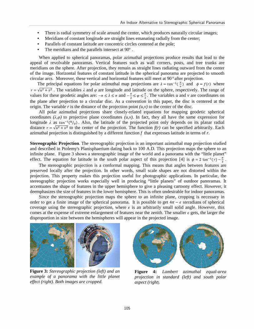
All polar azimuthal projections share closely-related equations for mapping geodetic spherical coordinates (λ,φ) to projective plane coordinates (u,v). In fact, they all have the same expression for longitude λ as ��(� �⁄ ). Also, the latitude of the projected point only depends on its planar radial distance � = √�� + �� to the center of the projection. The function f(r) can be specified arbitrarily. Each azimuthal projection is distinguished by a different function f that expresses latitude in terms of r. Stereographic Projection. The stereographic projection is an important azimuthal map projection studied and described in Ptolemy's Planisphaerium dating back to 100 A.D. This projection maps the sphere to an infinite plane. Figure 3 shows a stereographic image of the world and a panorama with the “little planet” effect. The equation for latitude in the south polar aspect of this projection [4] is = 2 tan��( �) − �

� . The stereographic projection is a conformal mapping. This means that angles between features are preserved locally after the projection. In other words, small scale shapes are not distorted within the projection. This property makes this projection useful for photographic applications. In particular, the stereographic projection works especially well in producing “little planets” of outdoor panoramas. It accentuates the shape of features in the upper hemisphere to give a pleasing cartoony effect. However, it deemphasizes the size of features in the lower hemisphere. This is often undesirable for indoor panoramas.

Since the stereographic projection maps the sphere to an infinite plane, cropping is necessary in order to get a finite image of the spherical panorama. It is possible to get 4� − steradians of spherical coverage using the stereographic projection, where is an arbitrarily small solid angle. However, this comes at the expense of extreme enlargement of features near the zenith. The smaller gets, the larger the disproportion in size between the hemispheres will appear in the projected image.

Figure 3: Stereographic projection (left) and an example of a panorama with the little planet effect (right). Both images are cropped.

Figure 4: Lambert azimuthal equal-area projection in standard (left) and south polar aspect (right).


105

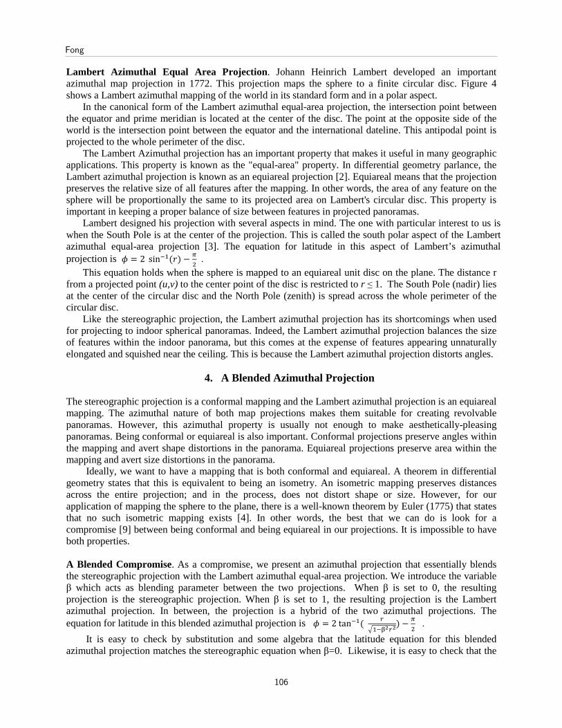
Lambert Azimuthal Equal Area Projection . Johann Heinrich Lambert developed an important azimuthal map projection in 1772. This projection maps the sphere to a finite circular disc. Figure 4 shows a Lambert azimuthal mapping of the world in its standard form and in a polar aspect.

In the canonical form of the Lambert azimuthal equal-area projection, the intersection point between the equator and prime meridian is located at the center of the disc. The point at the opposite side of the world is the intersection point between the equator and the international dateline. This antipodal point is projected to the whole perimeter of the disc.

The Lambert Azimuthal projection has an important property that makes it useful in many geographic applications. This property is known as the "equal-area" property. In differential geometry parlance, the Lambert azimuthal projection is known as an equiareal projection [2]. Equiareal means that the projection preserves the relative size of all features after the mapping. In other words, the area of any feature on the sphere will be proportionally the same to its projected area on Lambert's circular disc. This property is important in keeping a proper balance of size between features in projected panoramas.

Lambert designed his projection with several aspects in mind. The one with particular interest to us is when the South Pole is at the center of the projection. This is called the south polar aspect of the Lambert azimuthal equal-area projection [3]. The equation for latitude in this aspect of Lambert’s azimuthal projection is = 2 sin��(�) − �

� .

This equation holds when the sphere is mapped to an equiareal unit disc on the plane. The distance r from a projected point (u,v) to the center point of the disc is restricted to r ≤ 1. The South Pole (nadir) lies at the center of the circular disc and the North Pole (zenith) is spread across the whole perimeter of the circular disc.

Like the stereographic projection, the Lambert azimuthal projection has its shortcomings when used for projecting to indoor spherical panoramas. Indeed, the Lambert azimuthal projection balances the size of features within the indoor panorama, but this comes at the expense of features appearing unnaturally elongated and squished near the ceiling. This is because the Lambert azimuthal projection distorts angles.

4. A Blended Azimuthal Projection The stereographic projection is a conformal mapping and the Lambert azimuthal projection is an equiareal mapping. The azimuthal nature of both map projections makes them suitable for creating revolvable panoramas. However, this azimuthal property is usually not enough to make aesthetically-pleasing panoramas. Being conformal or equiareal is also important. Conformal projections preserve angles within the mapping and avert shape distortions in the panorama. Equiareal projections preserve area within the mapping and avert size distortions in the panorama.

Ideally, we want to have a mapping that is both conformal and equiareal. A theorem in differential geometry states that this is equivalent to being an isometry. An isometric mapping preserves distances across the entire projection; and in the process, does not distort shape or size. However, for our application of mapping the sphere to the plane, there is a well-known theorem by Euler (1775) that states that no such isometric mapping exists [4]. In other words, the best that we can do is look for a compromise [9] between being conformal and being equiareal in our projections. It is impossible to have both properties.

A Blended Compromise. As a compromise, we present an azimuthal projection that essentially blends the stereographic projection with the Lambert azimuthal equal-area projection. We introduce the variable β which acts as blending parameter between the two projections. When β is set to 0, the resulting projection is the stereographic projection. When β is set to 1, the resulting projection is the Lambert azimuthal projection. In between, the projection is a hybrid of the two azimuthal projections. The equation for latitude in this blended azimuthal projection is = 2tan��( #

$��%&#&) −�� .

It is easy to check by substitution and some algebra that the latitude equation for this blended azimuthal projection matches the stereographic equation when β=0. Likewise, it is easy to check that the

Fong

106

latitude equation for this blended azimuthal projection matches the Lambert azimuthal equation when β=1 by using the trigonometric identity sin��( �) = tan��(� √1 − ��⁄ ) . Normalized Form. The stereographic projection maps the sphere onto an infinite plane. In contrast, the Lambert azimuthal projection maps the sphere onto a finite circular disc. Needless to say, there is a wide disparity between the span of both projections. In order to have an effective blend of the two projections, we need a projection with a span that can grow from a finite disc to the infinite plane as β goes from 1 to 0. This is exactly what the blended azimuthal projection does - it grows infinitely in size as β approaches 0. In fact, the blended azimuthal projection maps the sphere to a disc with radius 1 β) .

The vast difference in the spanning range between the stereographic and the Lambert azimuthal projection adds difficulty in creating photographs from blending the two projections. We, therefore, propose a normalized form of the blended azimuthal projection. This normalization can be derived from its unnormalized latitude equation by writing r in terms of a normalized dummy variable defined as *+,,- = �., then renaming the dummy variable out of the equation. After this, the equation for latitude becomes = 2tan��( #

%$��#&) −�� .

This normalized form of the blended azimuthal projection effectively maps the sphere to a unit disc for all values of . ∈ (0,12. The only complication with this normalized form is that we are strictly restricted to have β > 0. That is, this projection cannot be set to 100% stereographic. This limitation stems from the difficulty of scaling down an infinite plane to a unit disc. Nevertheless, β can be set to an arbitrarily small number ε > 0 that can make the projection as close to stereographic as one wishes without actually setting β to zero. This helps us prevent division by zero and other undesirable infinities in the equations. Figure 6 shows the normalized blended azimuthal projection at different values of β from 0.1 to 1. In essence, this is like a sequence of frames of morphing from the nearly stereographic projection to the Lambert azimuthal equal-area projection.

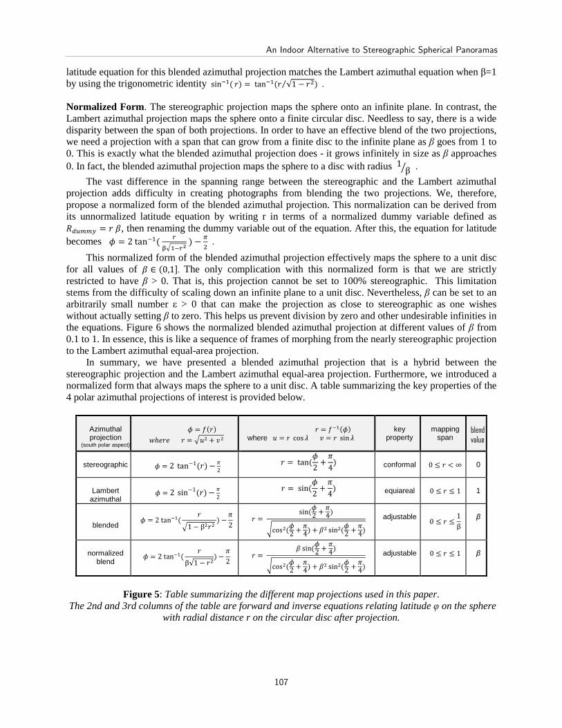
In summary, we have presented a blended azimuthal projection that is a hybrid between the stereographic projection and the Lambert azimuthal equal-area projection. Furthermore, we introduced a normalized form that always maps the sphere to a unit disc. A table summarizing the key properties of the 4 polar azimuthal projections of interest is provided below.

Figure 5: Table summarizing the different map projections used in this paper.

The 2nd and 3rd columns of the table are forward and inverse equations relating latitude φ on the sphere with radial distance r on the circular disc after projection.

Azimuthal projection

(south polar aspect)

= �(�)

3ℎ5�5� = $�� + ��

� = ��( )

where � = � cos � � = � sin�

key

property

mapping

span

blend

value

stereographic

= 2 tan−1(�) − �

2 � = tan( 2 + �

4)

conformal

0 ≤ � < ∞ 0

Lambert

azimuthal

= 2 sin−1(�) − �

2 � = sin( 2 + �4)

equiareal

0 ≤ � ≤ 1

1

blended

= 2tan��( �$1 − β��) −

�2

� = sin( 2 + �4):cos�( 2 + �4) + .� sin�( 2 + �4)

adjustable

0 ≤ � ≤ 1β

β

normalized

blend

= 2tan��( �β√1 − ��) −

�2

� = . sin( 2 + �4):cos�( 2 + �4) + .� sin�( 2 + �4)

adjustable

0 ≤ � ≤ 1 β


107

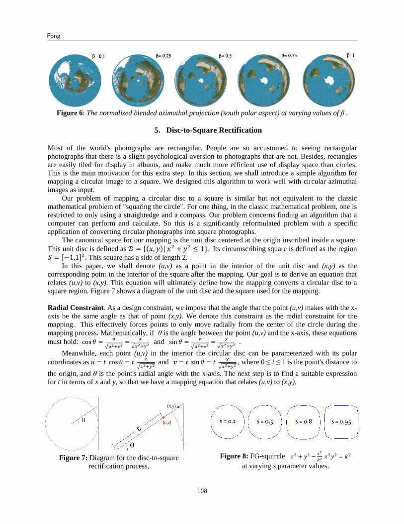
Figure 6: The normalized blended azimuthal projection (south polar aspect) at varying values of β .

5. Disc-to-Square Rectification Most of the world's photographs are rectangular. People are so accustomed to seeing rectangular photographs that there is a slight psychological aversion to photographs that are not. Besides, rectangles are easily tiled for display in albums, and make much more efficient use of display space than circles. This is the main motivation for this extra step. In this section, we shall introduce a simple algorithm for mapping a circular image to a square. We designed this algorithm to work well with circular azimuthal images as input.

Our problem of mapping a circular disc to a square is similar but not equivalent to the classic mathematical problem of "squaring the circle". For one thing, in the classic mathematical problem, one is restricted to only using a straightedge and a compass. Our problem concerns finding an algorithm that a computer can perform and calculate. So this is a significantly reformulated problem with a specific application of converting circular photographs into square photographs.

The canonical space for our mapping is the unit disc centered at the origin inscribed inside a square. This unit disc is defined as ; = <(=, >)|=� + >� ≤ 1}. Its circumscribing square is defined as the region A = B−1,12�. This square has a side of length 2.

In this paper, we shall denote (u,v) as a point in the interior of the unit disc and (x,y) as the corresponding point in the interior of the square after the mapping. Our goal is to derive an equation that relates (u,v) to (x,y). This equation will ultimately define how the mapping converts a circular disc to a square region. Figure 7 shows a diagram of the unit disc and the square used for the mapping. Radial Constraint. As a design constraint, we impose that the angle that the point (u,v) makes with the x-axis be the same angle as that of point (x,y). We denote this constraint as the radial constraint for the mapping. This effectively forces points to only move radially from the center of the circle during the mapping process. Mathematically, if θ is the angle between the point (u,v) and the x-axis, these equations must hold: cos C =

$&D�& = E$E&D-&and sin C = �

$&D�& = -$E&D-& .

Meanwhile, each point (u,v) in the interior the circular disc can be parameterized with its polar coordinates as � = � cos C = � E

$E&D-& and � = � sin C = � -$E&D-& , where 0 ≤ t ≤ 1 is the point's distance to

the origin, and θ is the point's radial angle with the x-axis. The next step is to find a suitable expression for t in terms of x and y, so that we have a mapping equation that relates (u,v) to (x,y).

Figure 7: Diagram for the disc-to-square rectification process.

Figure 8: FG-squircle =� + >� − F&

G& =�>� = H� at varying s parameter values.

Fong

108

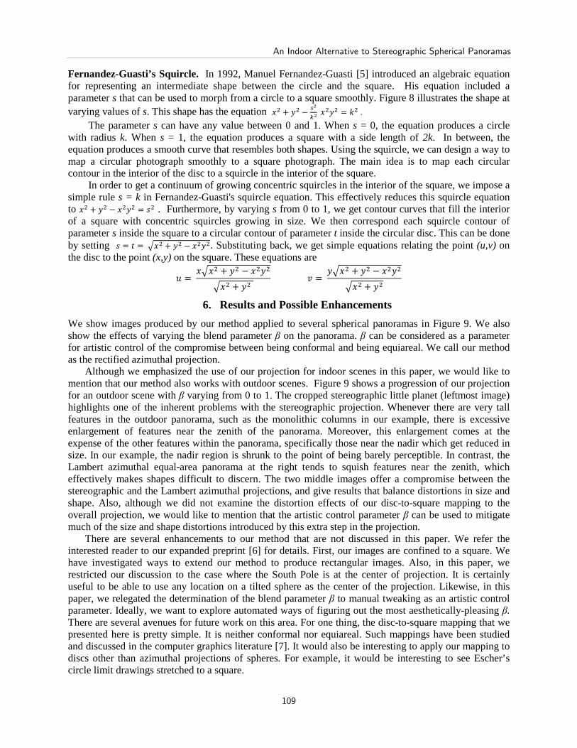
Fernandez-Guasti’s Squircle. In 1992, Manuel Fernandez-Guasti [5] introduced an algebraic equation for representing an intermediate shape between the circle and the square. His equation included a parameter s that can be used to morph from a circle to a square smoothly. Figure 8 illustrates the shape at varying values of s. This shape has the equation =� + >� − F&

G& =�>� = H�. The parameter s can have any value between 0 and 1. When s = 0, the equation produces a circle

with radius k. When s = 1, the equation produces a square with a side length of 2k. In between, the equation produces a smooth curve that resembles both shapes. Using the squircle, we can design a way to map a circular photograph smoothly to a square photograph. The main idea is to map each circular contour in the interior of the disc to a squircle in the interior of the square.

In order to get a continuum of growing concentric squircles in the interior of the square, we impose a simple rule s = k in Fernandez-Guasti's squircle equation. This effectively reduces this squircle equation to =� + >� − =�>� = I� . Furthermore, by varying s from 0 to 1, we get contour curves that fill the interior of a square with concentric squircles growing in size. We then correspond each squircle contour of parameter s inside the square to a circular contour of parameter t inside the circular disc. This can be done by setting I = � = $=� + >� − =�>�. Substituting back, we get simple equations relating the point (u,v) on the disc to the point (x,y) on the square. These equations are

� = =$=� + >� − =�>�

$=� + >� � = >$=� + >� − =�>�

$=� + >�

6. Results and Possible Enhancements

We show images produced by our method applied to several spherical panoramas in Figure 9. We also show the effects of varying the blend parameter β on the panorama. β can be considered as a parameter for artistic control of the compromise between being conformal and being equiareal. We call our method as the rectified azimuthal projection.

Although we emphasized the use of our projection for indoor scenes in this paper, we would like to mention that our method also works with outdoor scenes. Figure 9 shows a progression of our projection for an outdoor scene with β varying from 0 to 1. The cropped stereographic little planet (leftmost image) highlights one of the inherent problems with the stereographic projection. Whenever there are very tall features in the outdoor panorama, such as the monolithic columns in our example, there is excessive enlargement of features near the zenith of the panorama. Moreover, this enlargement comes at the expense of the other features within the panorama, specifically those near the nadir which get reduced in size. In our example, the nadir region is shrunk to the point of being barely perceptible. In contrast, the Lambert azimuthal equal-area panorama at the right tends to squish features near the zenith, which effectively makes shapes difficult to discern. The two middle images offer a compromise between the stereographic and the Lambert azimuthal projections, and give results that balance distortions in size and shape. Also, although we did not examine the distortion effects of our disc-to-square mapping to the overall projection, we would like to mention that the artistic control parameter β can be used to mitigate much of the size and shape distortions introduced by this extra step in the projection.

There are several enhancements to our method that are not discussed in this paper. We refer the interested reader to our expanded preprint [6] for details. First, our images are confined to a square. We have investigated ways to extend our method to produce rectangular images. Also, in this paper, we restricted our discussion to the case where the South Pole is at the center of projection. It is certainly useful to be able to use any location on a tilted sphere as the center of the projection. Likewise, in this paper, we relegated the determination of the blend parameter β to manual tweaking as an artistic control parameter. Ideally, we want to explore automated ways of figuring out the most aesthetically-pleasing β. There are several avenues for future work on this area. For one thing, the disc-to-square mapping that we presented here is pretty simple. It is neither conformal nor equiareal. Such mappings have been studied and discussed in the computer graphics literature [7]. It would also be interesting to apply our mapping to discs other than azimuthal projections of spheres. For example, it would be interesting to see Escher’s circle limit drawings stretched to a square.


109

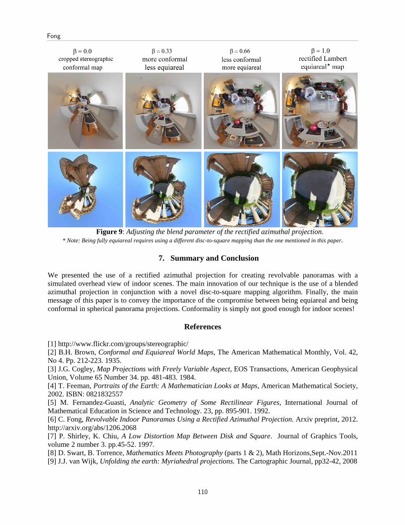
Figure 9: Adjusting the blend parameter of the rectified azimuthal projection. * Note: Being fully equiareal requires using a different disc-to-square mapping than the one mentioned in this paper.

7. Summary and Conclusion

We presented the use of a rectified azimuthal projection for creating revolvable panoramas with a simulated overhead view of indoor scenes. The main innovation of our technique is the use of a blended azimuthal projection in conjunction with a novel disc-to-square mapping algorithm. Finally, the main message of this paper is to convey the importance of the compromise between being equiareal and being conformal in spherical panorama projections. Conformality is simply not good enough for indoor scenes!

References

[1] http://www.flickr.com/groups/stereographic/ [2] B.H. Brown, Conformal and Equiareal World Maps, The American Mathematical Monthly, Vol. 42, No 4. Pp. 212-223. 1935. [3] J.G. Cogley, Map Projections with Freely Variable Aspect, EOS Transactions, American Geophysical Union, Volume 65 Number 34. pp. 481-483. 1984. [4] T. Feeman, Portraits of the Earth: A Mathematician Looks at Maps, American Mathematical Society, 2002. ISBN: 0821832557 [5] M. Fernandez-Guasti, Analytic Geometry of Some Rectilinear Figures, International Journal of Mathematical Education in Science and Technology. 23, pp. 895-901. 1992. [6] C. Fong, Revolvable Indoor Panoramas Using a Rectified Azimuthal Projection. Arxiv preprint, 2012. http://arxiv.org/abs/1206.2068 [7] P. Shirley, K. Chiu, A Low Distortion Map Between Disk and Square. Journal of Graphics Tools, volume 2 number 3. pp.45-52. 1997. [8] D. Swart, B. Torrence, Mathematics Meets Photography (parts 1 & 2), Math Horizons,Sept.-Nov.2011 [9] J.J. van Wijk, Unfolding the earth: Myriahedral projections. The Cartographic Journal, pp32-42, 2008

Fong

110

an indoor alternative to stereographic spherical...

Documents