An immersed boundary approach for thenumerical analysis of objects represented by

oriented point clouds

Laszlo Kudela∗1, Stefan Kollmannsberger1, and Ernst Rank1,2

1Chair for Computation in Engineering, Technical University of Munich, Arcisstr. 21, 80333 Munchen, Germany2Institute for Advanced Study, Technische Universitat Munchen, Germany

Abstract

This contribution presents a method aiming at the numerical analysis of solids whose boundaries arerepresented by oriented point clouds. In contrast to standard finite elements that require a boundary-conforming discretization of the domain of interest, our approach works directly on the point cloudrepresentation of the geometry. This is achieved by combining the inside-outside information thatis inferred from the members of the point cloud with a high order immersed boundary technique.This allows for avoiding the challenging task of surface fitting and mesh generation, simplifying theimage-based analysis pipeline drastically. We demonstrate by a numerical example how the proposedmethod can be applied in the context of linear elastostatic analysis of solids.

Keywords: image-based finite element analysis, point clouds, finite cell method

1 Introduction

A core challenge in the context of image-based finite element analysis revolves around the questionof how to derive an analysis-suitable finite element model from the point cloud data that describesthe shape of the domain of interest. Examples include the structural analysis of statues [1], historicalstructures [2, 3, 4] and the coupling of finite element computations to in vitro measurements ofbiological tissues [5]. In order to construct a finite-element mesh that resolves the boundaries ofthe geometry, the usual approach is to process the point cloud data through a multi-step pipelinethat results in a mesh of boundary-conforming finite elements. Generally, the main steps of suchcloud-to-analysis pipelines can be characterized as follows:

1. Geometry recoveryA geometric model is derived from the point cloud information using geometric segmentationand surface fitting techniques.

2. Mesh generationOnce the geometric representation of the object is recovered, the model is subdivided into aset of boundary-conforming finite elements.

3. Finite Element AnalysisThe mesh from the previous step together with the necessary material parameters and boundaryconditions is handed over to a finite element solver.

*laszlo.kudela@tum.de, Corresponding Author

Preprint accepted for publication in COMPIMAGE 2018 June 13, 2018

These steps are difficult to automate, as a solution which is tailored to a specific class of geometries isusually not directly applicable on other types of objects. Moreover, because the pipeline requires theinterplay of many techniques from computational science and engineering, the analyst performingthe above steps needs to be experienced with a wide variety of softwares and has to be aware oftheir respective pitfalls. For example, even if the geometry of the object is available through a CADmodel, the preparation of an analysis-suitable finite element mesh may require a great amount ofhuman interaction and can take up to 80% of the total analysis time [6].

In recent years, research efforts aiming at avoiding the difficult task of mesh generation broughtforth many approaches, such as the Finite Cell Method (FCM) introduced in [7]. The FCM relieson the combination of approaches well-known in computational mechanics: immersed boundary(IB) methods [8] and high-order finite elements (p-FEM) [9]. While initially suffering from lowaccuracy and high computational costs, IB methods have seen a complete revival in recent years.New numerical technologies addressing issues related to discretization [10], stability [11, 12], boundaryconditions [13] and numerical integration [14, 15, 16] allowed for the application of IB approaches innon-trivial fields. Examples include geometrically non-linear problems [17], plasticity [18], simulationof biomechanical structures [19], flow problems [20] and contact simulation [21].

Instead of generating a boundary-conforming discretization, FCM extends the physical domain ofinterest by a so-called fictitious domain, such that their union forms a simple bounding box thatcan be meshed easily. To keep the consistency with the original problem, the material parametersin the fictitious domain are penalized by a small factor α. The introduction of α shifts the analysiseffort from mesh generation to numerical integration. The biggest advantage of the FCM lies in highconvergence rates with almost no meshing costs.

In its simplest implementation, the only information that FCM needs from a geometric model isinside-outside state: given a point in space, does this point lie in the physical or the fictitious part ofthe domain? A wide variety of geometric representations is able to provide such point membershiptests and have been shown to work well in combination with the FCM, ranging from simple shapesto models as complex as metal foams.

In this contribution, the Finite Cell Method is combined with geometries that are represented byoriented point clouds. The members of the point cloud and the vectors associated to them provideenough information for point membership tests, allowing for simulating objects directly on theircloud representation. This way, the tedious tasks of recovering a geometric model and generating aboundary conforming mesh can be avoided. This allows for significant simplifications in the cloud-to-analysis pipeline.

2 The Finite Cell Method Combined with Oriented Point Clouds

In the following, the essential ideas of the Finite Cell Method for steady linear elastic problems arediscussed. For further details, see [7, 22].

2.1 A Brief Overview of FCM

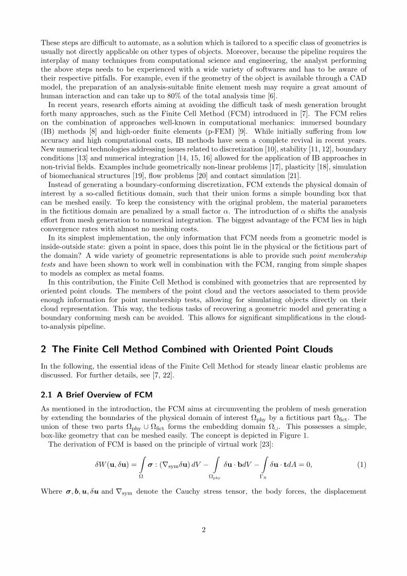
As mentioned in the introduction, the FCM aims at circumventing the problem of mesh generationby extending the boundaries of the physical domain of interest Ωphy by a fictitious part Ωfict. Theunion of these two parts Ωphy ∪ Ωfict forms the embedding domain Ω∪. This possesses a simple,box-like geometry that can be meshed easily. The concept is depicted in Figure 1.

The derivation of FCM is based on the principle of virtual work [23]:

δW (u, δu) =

∫Ω

σ : (∇symδu) dV −∫

Ωphy

δu · bdV −∫ΓN

δu · tdA = 0, (1)

Where σ, b,u, δu and ∇sym denote the Cauchy stress tensor, the body forces, the displacement

2

Ωphy

Ωfict

+ =

α = 0

α = 1

Ω∪t ΓN

ΓD

Figure 1: The core concept of the FCM. The physical domain Ωphy is extended by the fictitious domainΩfict. Their union, the embedding domain Ω∪ can be meshed easily. The influence of thefictitious domain is penalized by the scaling factor α.

vector, the test function and the symmetric part of the gradient, respectively. The traction vectort specifies the Neumann boundary conditions on ΓN. Stresses and strains are related through theconstitutive tensor C:

σ = αC : ε, (2)

where α is an indicator function defined as:

α(x) =

1 ∀x ∈ Ωphy

10−q ∀x ∈ Ωfict.(3)

In practice, the value of q is chosen between 6 and 12.Homogeneous Neumann boundary conditions are automatically satisfied by the formulation. Non-

homogeneous Neumann boundary conditions can be realized by evaluating the contour integral overΓN in Equation 1. Dirichlet boundary conditions are generally formulated in the weak sense, e.g.using the penalty method or Nitsche’s method [13].

The unknown quantities δu and u are discretized by a linear combination of Ni shape functionswith unknown coefficients ui:

u =∑i

Niui ; δu =∑i

Niδui, (4)

leading to the discrete finite cell representation:

Ku = f . (5)

In the standard version of FCM, integrated Legendre polynomials known from high-order finiteelements are employed as shape functions [22].

The stiffness matrix K results from a proper assembly of the element stiffness matrices:

ke =

∫Ωe

[LNe]T Cα [LNe] dΩe, (6)

where L is the standard strain-displacement operator, Ne is the matrix of shape functions associatedto the element and Cα = αC is the constitutive matrix.

In the context of FCM, the above integral is usually evaluated by means of specially constructedquadrature rules to account for the discontinuous integrand due to the scaling factor α. The mostpopular method is based on composed Gaussian quadrature rules combined with a recursive subdi-vision of the elements cut by the boundary of the physical domain. In this process, every intersectedelement is subdivided into equal subcells, until a pre-defined depth is reached. Quadrature points

3

Ω+i

Ω−i

pi,ni

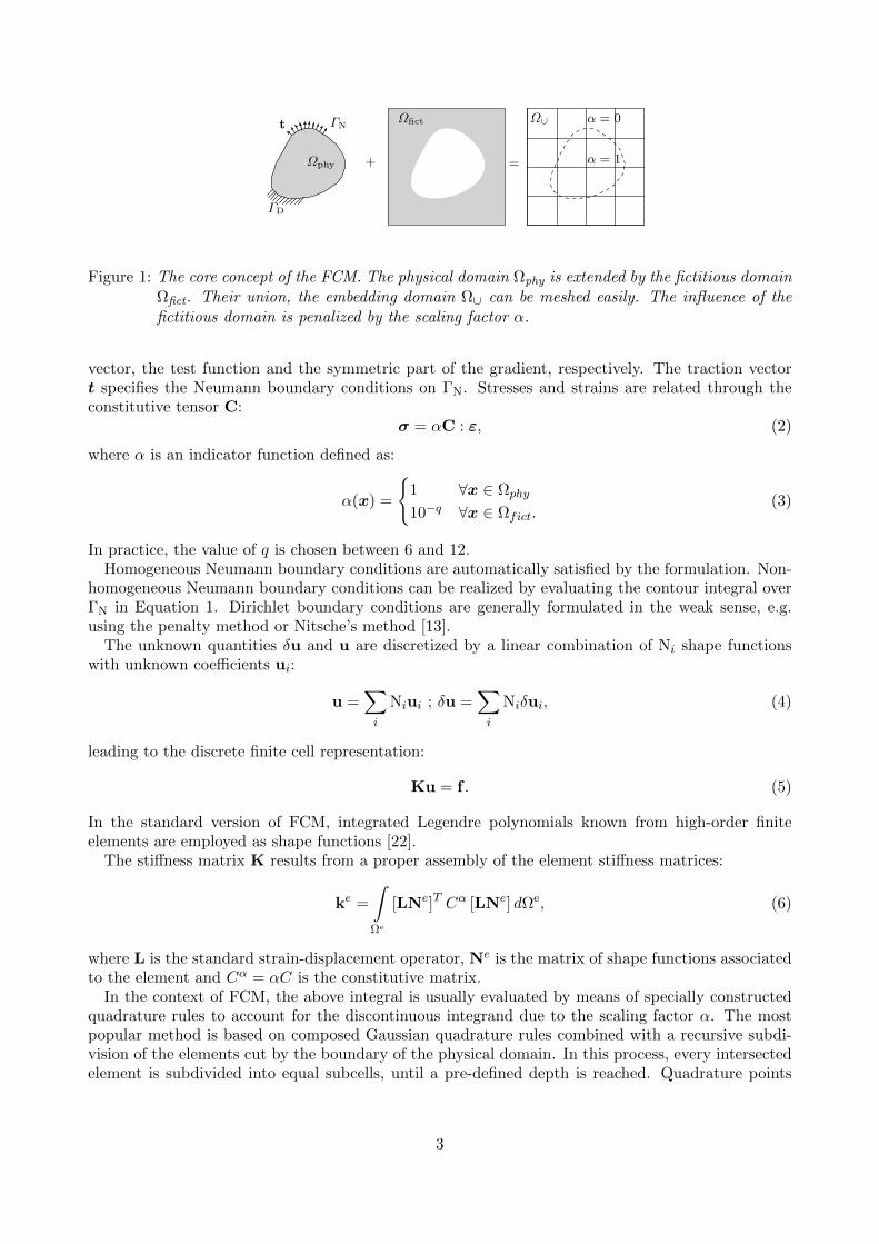
Figure 2: Point membership classification on oriented point clouds. The domain is represented bya set of points pi and associated normals ni. Every such pair locally separates the spacealong a hyperplane into two half-spaces: Ω−i and Ω+

i .

are then distributed on the domains of the leaf cells of this integration mesh.To compute the value of Cα for a given quadrature point, the indicator function in Equation 3

needs to be evaluated. This requires the geometric model that represents Ωphy to provide point-membership tests: given a quadrature point, does this point belong to Ωphy or not? Many geometricrepresentations are able to answer such inside-outside queries and have been successfully applied incombination with the FCM. Examples include voxel models from CT-scans [24], constructive solidgeometries [25], boundary representations [15] and STL descriptions [26].

2.2 Point Membership Tests on Oriented Point Clouds

In the context of point cloud based simulations, the domain Ωphy is represented by a set of samplepoints pi and their associated normal vectors ni. Assuming that no outliers are present, the set ofpairs S = pi,ni constitute a discrete sampling of the boundary ∂Ωphy of the domain.

Each element in S defines a hyperplane that separates the space in two half spaces: the openhalf-space Ω−i lying on the side of the hyperplane where the direction vector ni points, and the closedhalf-space Ω+

i lying on the other side. This concept is depicted in Figure 2. For every x ∈ Ω+i , the

following holds:(pi − x) · ni ≥ 0. (7)

Therefore, to determine whether a quadrature point q lies inside or outside the domain, it sufficesto find the pi and the associated ni in S that lies closest to q and evaluate the scalar product ofEquation 7. The algorithm requires an efficient nearest neighbor query. In our examples, we usethe k-d tree implementation from the Point Cloud Library [27]. The point membership classificationmethod is summarized in Algorithm 1.

Algorithm 1: Point membership test for oriented point clouds

1 function isPointInside (q, S) ;Input : Quadrature point q and oriented point cloud S = pi,niOutput: Boolean true if q lies inside the domain represented by S, false otherwise

2 pi,ni = getClosestPointInCloud(q, S);3 v = pi − q;4 d = v · ni;5 if d ≥ 0 then6 return true;7 end8 return false;

4

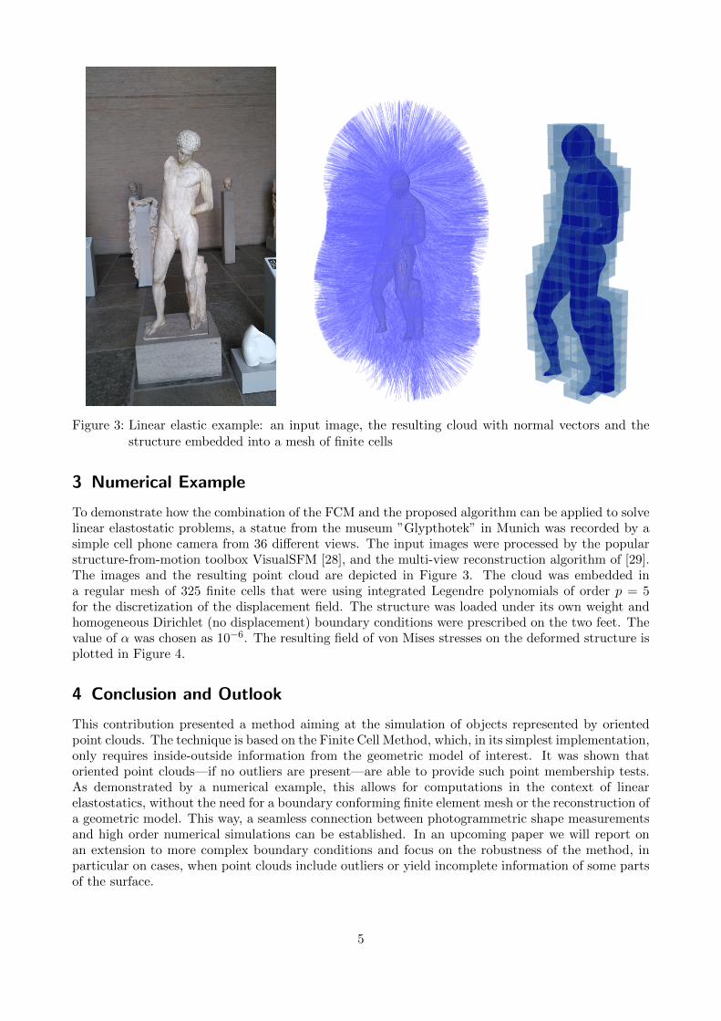
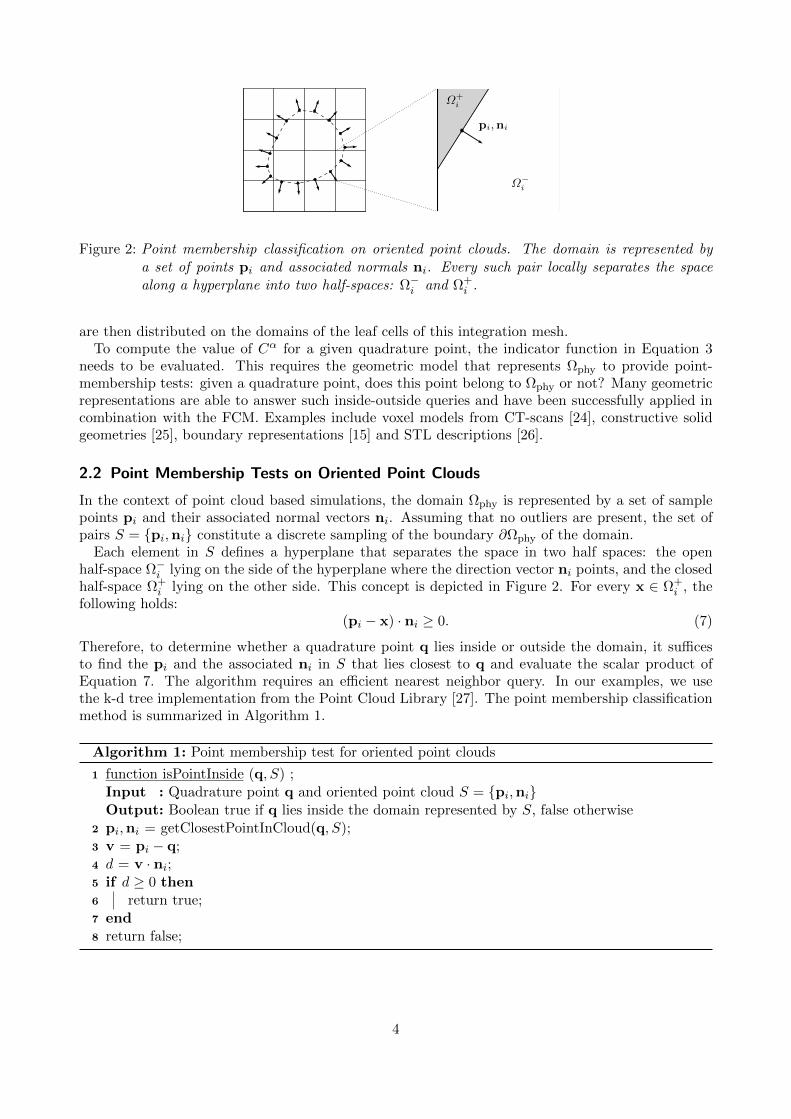
Figure 3: Linear elastic example: an input image, the resulting cloud with normal vectors and thestructure embedded into a mesh of finite cells

3 Numerical Example

To demonstrate how the combination of the FCM and the proposed algorithm can be applied to solvelinear elastostatic problems, a statue from the museum ”Glypthotek” in Munich was recorded by asimple cell phone camera from 36 different views. The input images were processed by the popularstructure-from-motion toolbox VisualSFM [28], and the multi-view reconstruction algorithm of [29].The images and the resulting point cloud are depicted in Figure 3. The cloud was embedded ina regular mesh of 325 finite cells that were using integrated Legendre polynomials of order p = 5for the discretization of the displacement field. The structure was loaded under its own weight andhomogeneous Dirichlet (no displacement) boundary conditions were prescribed on the two feet. Thevalue of α was chosen as 10−6. The resulting field of von Mises stresses on the deformed structure isplotted in Figure 4.

4 Conclusion and Outlook

This contribution presented a method aiming at the simulation of objects represented by orientedpoint clouds. The technique is based on the Finite Cell Method, which, in its simplest implementation,only requires inside-outside information from the geometric model of interest. It was shown thatoriented point clouds—if no outliers are present—are able to provide such point membership tests.As demonstrated by a numerical example, this allows for computations in the context of linearelastostatics, without the need for a boundary conforming finite element mesh or the reconstruction ofa geometric model. This way, a seamless connection between photogrammetric shape measurementsand high order numerical simulations can be established. In an upcoming paper we will report onan extension to more complex boundary conditions and focus on the robustness of the method, inparticular on cases, when point clouds include outliers or yield incomplete information of some partsof the surface.

5

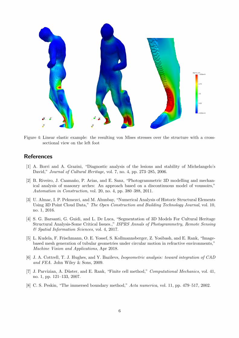
Figure 4: Linear elastic example: the resulting von Mises stresses over the structure with a cross-sectional view on the left foot

References

[1] A. Borri and A. Grazini, “Diagnostic analysis of the lesions and stability of Michelangelo’sDavid,” Journal of Cultural Heritage, vol. 7, no. 4, pp. 273–285, 2006.

[2] B. Riveiro, J. Caamano, P. Arias, and E. Sanz, “Photogrammetric 3D modelling and mechan-ical analysis of masonry arches: An approach based on a discontinuous model of voussoirs,”Automation in Construction, vol. 20, no. 4, pp. 380–388, 2011.

[3] U. Almac, I. P. Pekmezci, and M. Ahunbay, “Numerical Analysis of Historic Structural ElementsUsing 3D Point Cloud Data,” The Open Construction and Building Technology Journal, vol. 10,no. 1, 2016.

[4] S. G. Barsanti, G. Guidi, and L. De Luca, “Segmentation of 3D Models For Cultural HeritageStructural Analysis-Some Critical Issues.,” ISPRS Annals of Photogrammetry, Remote Sensing& Spatial Information Sciences, vol. 4, 2017.

[5] L. Kudela, F. Frischmann, O. E. Yossef, S. Kollmannsberger, Z. Yosibash, and E. Rank, “Image-based mesh generation of tubular geometries under circular motion in refractive environments,”Machine Vision and Applications, Apr 2018.

[6] J. A. Cottrell, T. J. Hughes, and Y. Bazilevs, Isogeometric analysis: toward integration of CADand FEA. John Wiley & Sons, 2009.

[7] J. Parvizian, A. Duster, and E. Rank, “Finite cell method,” Computational Mechanics, vol. 41,no. 1, pp. 121–133, 2007.

[8] C. S. Peskin, “The immersed boundary method,” Acta numerica, vol. 11, pp. 479–517, 2002.

6

[9] B. Szabo, A. Duster, and E. Rank, “The p-version of the finite element method,” Encyclopediaof computational mechanics, 2004.

[10] D. Schillinger, M. Ruess, N. Zander, Y. Bazilevs, A. Duster, and E. Rank, “Small and largedeformation analysis with the p-and B-spline versions of the finite cell method,” ComputationalMechanics, vol. 50, no. 4, pp. 445–478, 2012.

[11] F. de Prenter, C. Verhoosel, G. van Zwieten, and E. van Brummelen, “Condition number analysisand preconditioning of the finite cell method,” Computer Methods in Applied Mechanics andEngineering, vol. 316, pp. 297–327, 2017.

[12] E. Burman, S. Claus, P. Hansbo, M. G. Larson, and A. Massing, “CutFEM: Discretizing geom-etry and partial differential equations,” International Journal for Numerical Methods in Engi-neering, vol. 104, no. 7, pp. 472–501, 2015.

[13] M. Ruess, D. Schillinger, Y. Bazilevs, V. Varduhn, and E. Rank, “Weakly enforced essentialboundary conditions for NURBS-embedded and trimmed NURBS geometries on the basis ofthe finite cell method,” International Journal for Numerical Methods in Engineering, vol. 95,no. 10, pp. 811–846, 2013.

[14] T.-P. Fries and S. Omerovic, “Higher-order accurate integration of implicit geometries,” Inter-national Journal for Numerical Methods in Engineering, vol. 106, no. 5, pp. 323–371, 2016.

[15] L. Kudela, N. Zander, S. Kollmannsberger, and E. Rank, “Smart octrees: Accurately integrat-ing discontinuous functions in 3D,” Computer Methods in Applied Mechanics and Engineering,vol. 306, pp. 406–426, 2016.

[16] M. Joulaian, S. Hubrich, and A. Duster, “Numerical integration of discontinuities on arbitrarydomains based on moment fitting,” Computational Mechanics, vol. 57, no. 6, pp. 979–999, 2016.

[17] D. Schillinger, A. Duster, and E. Rank, “The hp-d-adaptive finite cell method for geometri-cally nonlinear problems of solid mechanics,” International Journal for Numerical Methods inEngineering, vol. 89, no. 9, pp. 1171–1202, 2012.

[18] A. Abedian, J. Parvizian, A. Duster, and E. Rank, “The finite cell method for the J2 flow theoryof plasticity,” Finite Elements in Analysis and Design, vol. 69, pp. 37–47, 2013.

[19] M. Elhaddad, N. Zander, T. Bog, L. Kudela, S. Kollmannsberger, J. Kirschke, T. Baum,M. Ruess, and E. Rank, “Multi-level hp-finite cell method for embedded interface problemswith application in biomechanics,” International Journal for Numerical Methods in BiomedicalEngineering, vol. 34, no. 4, p. e2951.

[20] F. Xu, D. Schillinger, D. Kamensky, V. Varduhn, C. Wang, and M.-C. Hsu, “The tetrahe-dral finite cell method for fluids: Immersogeometric analysis of turbulent flow around complexgeometries,” Computers & Fluids, vol. 141, pp. 135–154, 2016.

[21] T. Bog, N. Zander, S. Kollmannsberger, and E. Rank, “Weak imposition of frictionless con-tact constraints on automatically recovered high-order, embedded interfaces using the finite cellmethod,” Computational Mechanics, vol. 61, no. 4, pp. 385–407, 2018.

[22] A. Duster, E. Rank, and B. Szabo, “The p-Version of the Finite Element and Finite Cell Meth-ods,” Encyclopedia of Computational Mechanics Second Edition, 2017.

[23] T. J. R. Hughes, The Finite Element Method: Linear Static and Dynamic Finite Element Anal-ysis. Dover Publications, 2000.

7

[24] M. Ruess, D. Tal, N. Trabelsi, Z. Yosibash, and E. Rank, “The finite cell method for bonesimulations: verification and validation,” Biomechanics and modeling in mechanobiology, vol. 11,no. 3-4, pp. 425–437, 2012.

[25] B. Wassermann, S. Kollmannsberger, T. Bog, and E. Rank, “From geometric design to numericalanalysis: A direct approach using the Finite Cell Method on Constructive Solid Geometry,”Computers & Mathematics with Applications, vol. 74, no. 7, pp. 1703–1726, 2017.

[26] M. Elhaddad, N. Zander, S. Kollmannsberger, A. Shadavakhsh, V. Nubel, and E. Rank, “Finitecell method: High-order structural dynamics for complex geometries,” International Journal ofStructural Stability and Dynamics, p. 1540018, 2015.

[27] R. B. Rusu and S. Cousins, “3D is here: Point Cloud Library (PCL),” in IEEE InternationalConference on Robotics and Automation (ICRA), (Shanghai, China), May 9-13 2011.

[28] C. Wu et al., “VisualSFM: A visual structure from motion system,”

[29] Y. Furukawa and J. Ponce, “Accurate, dense, and robust multiview stereopsis,” IEEE transac-tions on pattern analysis and machine intelligence, vol. 32, no. 8, pp. 1362–1376, 2010.

8