an idealized model of tidal dynamics in the north sea ... · an idealized model of tidal dynamics...
TRANSCRIPT
Ocean Dynamics (2011) 612019ndash2035DOI 101007s10236-011-0456-x
An idealized model of tidal dynamics in the North Searesonance properties and response to large-scale changes
Pieter C Roos middot Jorick J Velema middotSuzanne J M H Hulscher middot Ad Stolk
Received 29 March 2011 Accepted 13 June 2011 Published online 19 July 2011copy The Author(s) 2011 This article is published with open access at Springerlinkcom
Abstract An idealized process-based model is devel-oped to investigate tidal dynamics in the North SeaThe model geometry consists of a sequence of differentrectangular compartments of uniform depth thus ac-counting for width and depth variations in a stepwisemanner This schematization allows for a quick andtransparent solution procedure The solution forcedby incoming Kelvin waves at the open boundaries andsatisfying the linear shallow water equations on thef plane with bottom friction is in each compartmentwritten as a superposition of eigenmodes ie Kelvinand Poincareacute waves A collocation method is employedto satisfy boundary and matching conditions First thegeneral resonance properties of a strongly simplifiedgeometry with two compartments representing theNorthern North Sea and Southern Bight are studiedVarying the forcing frequency while neglecting bot-tom friction reveals Kelvin and Poincareacute resonanceThese resonances continue to exist (but with loweramplification and a modified spatial structure) whenadding the Dover Strait as a third compartment andseparating the solutions due to forcing from either
Responsible Editor Joachim W Dippner
P C Roos (B) middot J J Velema middot S J M H HulscherDepartment of Water Engineering and ManagementFaculty of Engineering Technology University of TwentePO Box 217 7500 AE Enschede The Netherlandse-mail pcroosutwentenl
A StolkRijkswaterstaat Noordzee Ministry of Infrastructureand the Environment PO Box 5807 2280 HV RijswijkThe Netherlands
the north or the south only Including bottom frictiondampens the peaks Next comparison with tide ob-servations along the North Sea coast shows remark-able agreement for both semi-diurnal and diurnal tidesThis result is achieved with a more detailed geometryconsisting of 12 compartments fitted to the coastlineof the North Sea Further simulations emphasize theimportance of Dover Strait and bottom friction Finallyit is found that a sea level rise of 1 m uniformly appliedto the entire North Sea amplifies the M2-elevationamplitudes almost everywhere along the coast withan increase of up to 8 cm in Dover Strait Bed levelchanges of plusmn1 m uniformly applied to the SouthernBight only imply weaker changes with changes incoastal M2-elevation amplitudes below 5 cm
Keywords Tides middot North Sea middot Resonance middotSea level rise
1 Introduction
Understanding tidal dynamics in the North Sea is im-portant for navigation coastal safety and ecology Thislink is both direct through fluctuating water levels andoscillatory currents and indirect through the dynamicsof tide-induced bed forms (Dyer and Huntley 1999)Of particular interest is the tidersquos response to large-scale changes due to human intervention (de Boer et al2011) and sea level rise
Tide observations in the North Sea indicate a pre-dominant semi-diurnal character (Otto et al 1990Huthnance 1991) Semi-diurnal lunar (M2) elevationamplitudes are of the order of 1 m Diurnal componentsare weaker with coastal elevation amplitudes of K1
2020 Ocean Dynamics (2011) 612019ndash2035
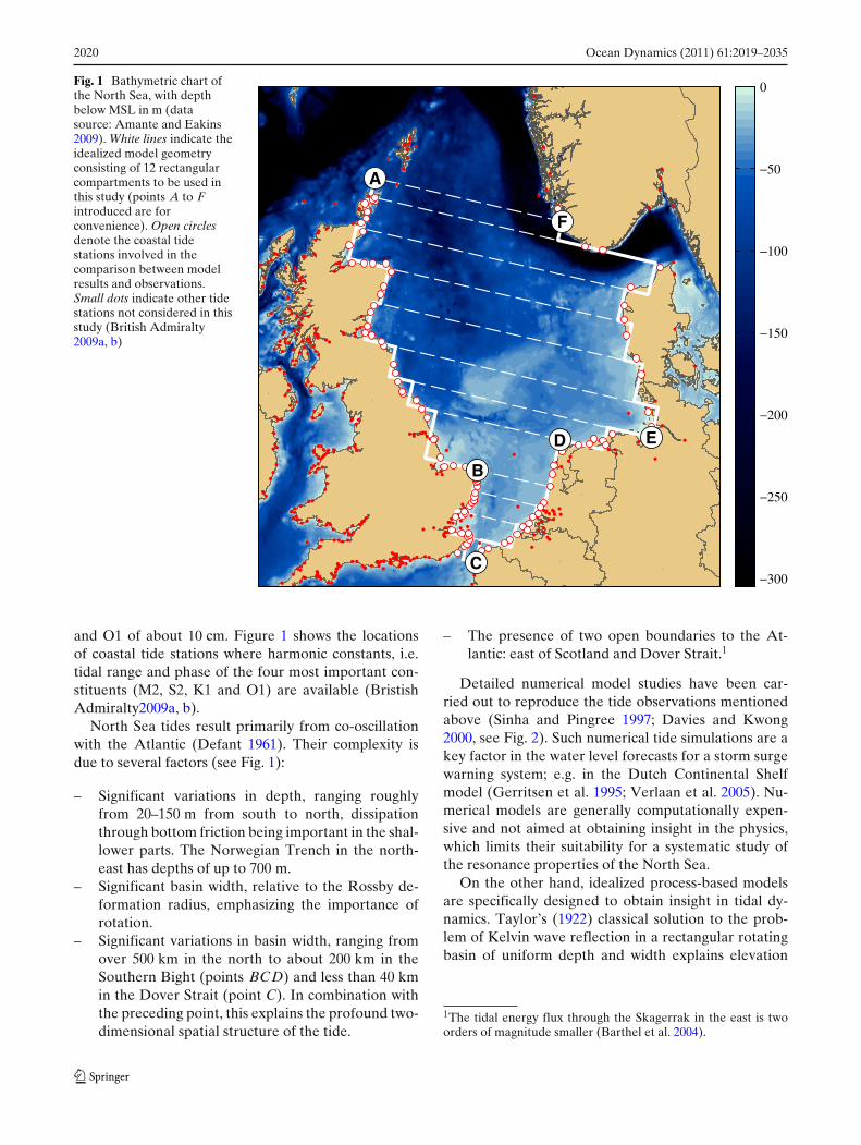
Fig 1 Bathymetric chart ofthe North Sea with depthbelow MSL in m (datasource Amante and Eakins2009) White lines indicate theidealized model geometryconsisting of 12 rectangularcompartments to be used inthis study (points A to Fintroduced are forconvenience) Open circlesdenote the coastal tidestations involved in thecomparison between modelresults and observationsSmall dots indicate other tidestations not considered in thisstudy (British Admiralty2009a b)
A
B
C
D E
F
minus300
minus250
minus200
minus150
minus100
minus50
0
and O1 of about 10 cm Figure 1 shows the locationsof coastal tide stations where harmonic constants ietidal range and phase of the four most important con-stituents (M2 S2 K1 and O1) are available (BristishAdmiralty2009a b)
North Sea tides result primarily from co-oscillationwith the Atlantic (Defant 1961) Their complexity isdue to several factors (see Fig 1)
ndash Significant variations in depth ranging roughlyfrom 20ndash150 m from south to north dissipationthrough bottom friction being important in the shal-lower parts The Norwegian Trench in the north-east has depths of up to 700 m
ndash Significant basin width relative to the Rossby de-formation radius emphasizing the importance ofrotation
ndash Significant variations in basin width ranging fromover 500 km in the north to about 200 km in theSouthern Bight (points BCD) and less than 40 kmin the Dover Strait (point C) In combination withthe preceding point this explains the profound two-dimensional spatial structure of the tide
ndash The presence of two open boundaries to the At-lantic east of Scotland and Dover Strait1
Detailed numerical model studies have been car-ried out to reproduce the tide observations mentionedabove (Sinha and Pingree 1997 Davies and Kwong2000 see Fig 2) Such numerical tide simulations are akey factor in the water level forecasts for a storm surgewarning system eg in the Dutch Continental Shelfmodel (Gerritsen et al 1995 Verlaan et al 2005) Nu-merical models are generally computationally expen-sive and not aimed at obtaining insight in the physicswhich limits their suitability for a systematic study ofthe resonance properties of the North Sea
On the other hand idealized process-based modelsare specifically designed to obtain insight in tidal dy-namics Taylorrsquos (1922) classical solution to the prob-lem of Kelvin wave reflection in a rectangular rotatingbasin of uniform depth and width explains elevation
1The tidal energy flux through the Skagerrak in the east is twoorders of magnitude smaller (Barthel et al 2004)
Ocean Dynamics (2011) 612019ndash2035 2021
Fig 2 Co-tidal charts of M2-tide (left) and K1-tide (right) with elevation amplitudes in cm (solid) and phases in degrees (dashed) asobtained with a numerical model (Davies and Kwong 2000 reprinted with permission from the American Geophysical Union)
amphidromic points (no surface fluctuations) and cur-rent amphidromic points (no velocities) occurring al-ternately on the centerline of the basin Incorporatingdissipation causes the amphidromes to shift in the cross-basin direction (Rienecker and Teubner 1980 Rizal2002 Roos and Schuttelaars 2009) To mimic DoverStrait Brown (1987 1989) imposed an oscillating freesurface elevation at the head which causes an along-basin shift of the amphidromes We note that also com-plex numerical models have been run with simplifiedgeometries to study the frictional and wind effects witha three-dimensional model (Davies and Jones 19951996) the influence of basin geometry on the currentamphidromic system (Xia et al 1995) and sandbankformation (Carbajal et al 2005) Table 1 summarizesthe tidal basins around the world that have been studiedusing (extensions of) Taylorrsquos (1922) idealized modelAlthough the idealized studies mentioned above pro-vide qualitative insight the rather strong geometricalschematizations preclude a more specific understand-ing of the North Sea tides
A third class of studies specifically focused on theresonance properties of tidal basins which is indica-tive of their response to large-scale changes A clas-sical result for semi-enclosed bays co-oscillating witha larger seaocean states that resonance occurs when
basin length equals one quarter of the shallow wa-ter wavelength (or an odd multiple see eg Defant1961) This theory however ignores radiative dampinginto the adjacent seaocean (Garrett 1975) and is onlyvalid for narrow rectangular bays of uniform depth andwidth Rotation complicates the resonance propertiesof wider basins which also allow for a cross-bay half-wave2 resonance (Huthnance 1980)3 This type of reso-nance associated with amplification of Poincareacute modesis also possible in wide embayments of uniform widthwith a shallow zone near the head (Webb 1976 Roosand Schuttelaars 2011) Alternatively the resonantfrequencies of various basins around the world havebeen estimated by fitting analytical frequency-responsecurves to tide observations (Garrett 1972 Godin 1993Sutherland et al 2005 Arbic et al 2007) The curves arederived from eg the rectangular bay model mentionedabove (or a Helmholtz oscillator for smaller basins)
2Or an integer multiple of this one half wave one wave threehalve waves etc3Huthnance (1980) used the term lsquoresonancersquo only to denoteinf inite amplification and uses lsquomaximum responsersquo in the caseof a peak that is finite due to friction radiation damping androtation In the present study we use the term lsquoresonancersquo todenote any peak response
2022 Ocean Dynamics (2011) 612019ndash2035
Table 1 Overview of studies extending Taylorrsquos (1922) approach and applying it to basins other than the North Sea
Reference Application Constituent(s) Comp Width Bottomvariations friction
Godin (1965) Labrador SeaDavis StrBaffin Bay M2 3 Yes NoHendershott and Speranza (1971) Adriatic Sea Gulf of California M2 1a No Noab
Webb (1976) Patagonian Shelf M2c 2 No YesKowalik (1979) Arctic Sea M2 2d nad YesHuthnance (1980) Brazilian shelf M3 2e Yese YesKang (1984) Yellow Sea M2 K1 1f No NoMosetti (1986) Northern Adriatic M2 1 No NoYanagi (1987) Bungo and Kii Channel (Japan) M2 1a No NoFang et al (1991) Yellow Sea M2 1fg No YesRizal (2000) Malacca Strait M2 1 No YesJung et al (2005) Yellow Sea East China Sea M2 3g No YesRoos and Schuttelaars (2011) Adr Sea Gulf of Cal Persian Gulf M2 S2 K1 O1 2 3h No Yes
aSuperposition of two Kelvin waves without bottom frictionbPartial absorption at bay head a region not explicitly resolved explains the amplitude reduction and phase lag of the reflected KelvinwavecThe systemrsquos resonant period is estimated at 108 h (223 cpd) near the semi-diurnal band forcing frequency further treated as acomplex quantitydFrictionless Kelvin wave in channel Sverdrup wave in circular basinrsquos interior no systematic matching of these two solutionseExtending Garrettrsquos (1975) analysis to wide gulfs explaining ocean-shelf resonancefPart of bay head as open boundarygSpecifying elevation amplitude at bay mouth (rather than sending in a Kelvin wave)hAlso allowing for transverse topographic steps
whereas the observations comprise amplitude gains andphase shifts over the basin for various tidal constituentsThis method relies on the availability of observations atdifferent tidal frequencies their proximity to resonanceand the validity of the model underlying the adoptedfrequency-response curve
The present study is aimed at understanding tidaldynamics in the North Sea particularly its resonanceproperties and its response to large-scale changes Mo-tivated by the lack of geometrical detail in existingidealized model studies and the limited suitability ofnumerical models for this purpose we present a newidealized model (Fig 1) Innovative aspects of our workare the model geometry (many compartments depthand width variations two open boundaries) the focuson resonance properties and the detailed comparisonwith semi-diurnal and diurnal tide observations alongthe North Sea coast Our approach largely follows thatof Roos and Schuttelaars (2011) but involves the neces-sary extensions to make it suitable for the North Sea
This paper is organized as follows The model set-up and solution method are presented in Section 2 InSection 3 we investigate the general resonance prop-erties of a relatively shallow compartment connectedto a wider and deeper compartment and to a narrowstrait A crucial next step is then to show that our modelis quantitatively capable of reproducing tidal dynamicsas observed in the North Sea (tide stations in Fig 1)As shown in Section 4 good agreement with semi-
diurnal and diurnal tide observations is achieved witha geometry consisting of 12 compartments This resultgives confidence in the modelrsquos reliability in situationsfor which no observational data are available Furthersimulations presented in Section 5 then provide insightinto
ndash The importance of the tidal energy fluxes from thenorth (east of Scotland) and the south (throughDover Strait) as well as the effects of closure ofDover Strait
ndash The role of bottom frictionndash The effects of sea level rise simulated by an overall
increase in water depthndash The systemrsquos sensitivity to bed level variations in
the Southern Bight
Finally Sections 6 and 7 contain the discussion andconclusions respectively
2 Model
21 Model formulation
Consider a tidal wave of angular frequency ω andtypical elevation amplitude Z The model geometryconsists of a sequence of J rectangular compartmentsof length l j width b j and (uniform) depth h j (Fig 3)The geometries in Fig 3a b will be used in Section 3
Ocean Dynamics (2011) 612019ndash2035 2023
h1
h2 l2
l1
bb
2
1
(a) Two compartments
h3b3 l3
(b) Three compartments (including strait)
hj lj
bj
xy
(c) North Sea fit
Fig 3 Definition sketch of the model geometry showing a a simple set-up with two compartments b extension with strait and c theNorth Sea fit with 12 compartments also shown in Figs 1 and 6 Shaded compartments represent the Southern Bight details in Table 3
to investigate general resonance properties The moredetailed geometry in Fig 3c will be used in Section 4 toreproduce tide observations in the North Sea and formsthe basis of further simulations in Section 5 Detailsof these configurations are given in Table 3 where δ j
denotes the displacement of compartment jrsquos centerlinewith respect to that of compartment j minus 1
The compartment widths are not small comparedwith the (local) Rossby deformation radius whichshows the importance of adopting a horizontally two-dimensional approach including rotation Assumingthat Zh j 1 conservation of momentum and mass isexpressed by the depth-averaged linear shallow waterequations on the f plane4
partu j
parttminus f jv j + r ju j
h j= minusg
partη j
partx (1)
partv j
partt+ f ju j + r jv j
h j= minusg
partη j
party (2)
partη j
partt+ h j
[partu j
partx+ partv j
party
]= 0 (3)
For compartment j u j and v j are the depth-averagedflow velocity components in along-basin x and cross-basin y-direction respectively and η j is the free surfaceelevation ( j = 1 middot middot middot J) Furthermore f j = 2 sin ϑ j isa Coriolis parameter (with = 7292 times 10minus5 rad sminus1
the angular frequency of the Earthrsquos rotation and ϑ j thecentral latitude of compartment j) and g = 981 m sminus2
4For a derivation of Eqs1ndash3 see eg the scaling procedure inRoos and Schuttelaars (2009)
the gravitational acceleration Finally we have intro-duced a bottom friction coefficient
r j = 8cD〈U j〉3π
〈U j〉 = αFU j (4)
based on linearization of a quadratic friction law whileaccounting for the simultaneous presence of severaltidal components In Eq 4 cD = 25 times 10minus3 is a stan-dard drag coefficient Furthermore the velocity scale〈U j〉 is a correction of the coastal current amplitude U j
of a classical Kelvin wave without bottom friction (Gill1982)
U j = ZM2
radicgh j
(5)
Here the coastal elevation amplitude ZM2 = 140 m istypical for the dominant M2-tide obtained by averag-ing over all coastal tide stations under consideration
Turning back to Eq 4 the following corrections aremade to U j to obtain a proper velocity scale 〈U j〉Firstly the coefficient α accounts for the fact that cur-rent amplitudes throughout the domain are typicallysmaller than the tidal current amplitudes near the coast(α lt 1) In Section 4 α will be used as a tuning pa-rameter that is assumed identical for all constituentsSecondly the coefficient F accounts for the fact thatthe simultaneous presence of several tidal componentsenhances friction (F gt 1) particularly for the weakercomponents (Jeffreys 1970 Pingree 1983 Inoue andGarrett 2007) Properly incorporating this mechanismis important when we use our model to reproduce tideobservations in Section 4 To calculate the F values forM2 S2 K1 and O1 in the North Sea we follow the
2024 Ocean Dynamics (2011) 612019ndash2035
procedure by Inoue and Garrett (2007) see Table 2and Appendix A As it turns out the ratios FFM2
are close to the theoretical maximum of 15 obtainedin the ε darr 0-limit with ε = ZZM2 (Jeffreys 1970) InSection 3 where we investigate the modelrsquos frequencyresponse by varying ω in a broad range surroundingthe tidal bands we will ignore the presence of othercomponents and take F = 1
Our model geometry displays different types ofboundaries At the closed boundaries Bu j and Bv j
orthogonal to the along-basin and cross-basin directionrespectively we impose a no-normal flow condition ie
u j = 0 for (x y) isin Bu j (6)
v j = 0 for (x y) isin Bv j (7)
Next continuity of elevation and normal flux is re-quired across the topographic steps I j j+1 between theadjacent compartments
h ju j = h j+1u j+1 η j = η j+1 for (x y) isin I j j+1
(8)
Finally the system is forced by a single Kelvin wavecoming in through the open boundary for the geometryin Fig 3a or by two Kelvin waves coming in through thetwo open boundaries for the geometries in Fig 3b c Ineither case other waves are allowed to radiate outwardIn the case of two incoming Kelvin waves the solutionwill also depend on their relative amplitudes and phaselag which complicates the interpretation of the modelresults
22 Solution method
Let φ equiv (u v η) symbolically denote the solution Ineach compartment we seek time-periodic solutions ofthe form
φ j equiv (u j v j η j) = (u j v j η j) exp(iωt)
(9)
Table 2 Amplitudes Z and friction coefficients F as used inEq 4 of four tidal components in the North Sea
Comp T (h) ω (cpd)a Z (m)b ε (minus)c F (minus) FFM2 (minus)
M2 1242 1932 140 ndash 1078 1S2 1200 2000 043 0307 1522 141K1 2393 1003 009 0064 1539 143O1 2582 0930 011 0079 1538 143
aTidal frequency in cycles per daybElevation amplitude obtained by averaging over coastal tidestationscAmplitude divided by (dominant) M2-amplitude ie ε =ZZM2
with denoting the real part ω the angular frequencyand (u j v j η j) the complex amplitudes of flow andelevation which depend on x and y These amplitudesare then written as a truncated superposition of funda-mental wave solutions in an open channel ie Kelvinand Poincareacute modes propagating or exponentially de-caying in the positive and negative x-direction (seeAppendix B) Since these individual waves satisfy thelateral boundary condition in Eq 7 so does their su-perposition in the solution
A collocation technique is then employed to alsosatisfy the other no-normal flow condition in Eq 6and the matching conditions in Eq 8 We thus extendearlier studies to account for width variations (Webb1976 Jung et al 2005 Roos and Schuttelaars 2011)Collocation points are defined with an equidistant spac-ing along the interfaces and the adjacent closed lon-gitudinal boundaries5 At each collocation point werequire either zero normal flow (if located on a closedboundary) or matching of elevation and normal flux(if located on an interface) The truncation numbersmentioned previously are chosen such to balance thedistribution of collocation points The coefficients ofthe individual modes then follow from a linear systemwhich is solved using standard techniques
In the remainder of this study we adopt an averagespacing between collocation points of about 6 km InSection 3 where we investigate the resonance proper-ties of the simple geometries in Fig 3a b this leadsto a total number of about 170 Kelvin and Poincareacutemodes In reproducing the tide observations from theNorth Sea (Section 4 geometry of Fig 3c) the samespacing implies a total number of about 1700 Kelvinand Poincareacute modes in the complete domain
3 Results general resonance properties
31 Indicators of amplitude gain in the Southern Bight
To investigate resonance properties we consider thefrequency-response of our model To this end we an-alyze the solution for different values of the forcing fre-quency ω in a range that includes the diurnal and semi-diurnal tidal bands This analysis will be carried out forthe simple geometries shown in Fig 3a b The first con-sists of two compartments representing the relativelywide and deep northern part of the North Sea and the
5The open boundaries do not require collocation points since wespecify incoming Kelvin waves
Ocean Dynamics (2011) 612019ndash2035 2025
Table 3 Compartment properties of the basin geometries inFig 3
Fig j l j (km) b j (km) h j (m) δ j (km)a ϑ j (N)
3a 1 600 550 80 ndash 562b 200 200 20 0 52
3b 1 600 550 80 ndash 562b 200 200 20 0 523 40 35 20 0 51
3c 1 50 500 1515 ndash 5902 85 760 1299 minus130 5813 85 720 738 40 5744 95 650 650 minus72 5655 100 720 529 minus16 5566 80 700 413 minus74 5477 60 520 396 27 5418 125 330 267 19 5339b 55 190 263 minus70 524
10b 60 170 249 10 51911b 60 160 195 35 51512 60 35 273 18 510
aDisplacement in y-direction of the centerline of compartment jwith respect to that of compartment j minus 1bCompartment(s) representing the Southern Bight (shaded inFig 3)
narrower and shallower Southern Bight This geometryis extended in Fig 3b by including a third compartmentrepresenting Dover Strait as a second opening to theAtlantic For simplicity all compartments have beensymmetrically aligned about the basinrsquos central axis ieδ j = 0 See Table 3 for the dimensions and latitudes
To quantify the lsquoresponsersquo we introduce the ampli-tude gain Ahead This indicator is defined as the eleva-tion amplitude scaled against the input amplitude Z inc
and averaged over the head of the bight (thick solid linein Fig 3a)
Ahead = 1
b 2 Z inc
int|η2|dy (10)
Although Ahead is commonly used to quantify the am-plitude gain (eg Huthnance 1980) it is less meaningfulfor the case with a strait because part of the bay headis then an open boundary (Fig 3b) We thereforeintroduce a second indicator Abight averaging the ele-vation amplitude over the complete bight (shaded areain Fig 3a b)
Abight = 1
b 2l2 Z inc
intint|η2|dx dy (11)
32 Results for two compartments
Figure 4a shows the amplitude gains Ahead and Abight
as a function of forcing frequency for the two-compartment geometry (Fig 3a) both without and withbottom friction It is seen that both amplitude gainsshow qualitatively similar behaviour with as one mayexpect the bight-averaged indicator Abight (red line)being somewhat lower than the head-averaged Ahead
(black line)
1 2 3 4 50
1
2
3
4
5(a) Two compartments
ω (cpd)
Am
plitu
de g
ain
(minus)
a
b
c
d
1 2 3 4 50
1
2
3
4
5
e
f
g
h
i j
k
l
(b) Three compartments (including strait)
ω (cpd)
Am
plitu
de g
ain
(minus)
Fig 4 Amplitude gain versus forcing frequency ω for the modelgeometries in Fig 3a b a two compartments b three com-partments (including strait) Solid lines without bottom frictiondashed lines with bottom friction In (a) the black and red linesindicate Ahead and Abight respectively In (b) the red and blue
lines indicate Abight(N) and Abight(S) respectively ie separatelyforcing the system from the north and south only The co-tidalcharts of the cases denoted by the lowercase letters andashl aredepicted in Fig 5
2026 Ocean Dynamics (2011) 612019ndash2035
The curves without bottom friction (solid lines) dis-play a peak between the diurnal band (ω asymp 1 cpd) andsemi-diurnal band (ω asymp 2 cpd) a weaker response atω = 25 minus 3 cpd and two further peaks at higher valuesof the forcing frequency As can be seen from the co-tidal chart in Fig 5a the first peak is associated with aquarter wavelength resonance of the Kelvin mode inthe Southern Bight Next Fig 5b shows an example ofweaker amplification in the bight which is accompa-nied by higher amplitudes in the corners of the deepand wide compartment (eg the German Bight regionnear point E in Fig 1) The second peak in thefrequency-response curve represents resonance of the
first Poincareacute mode (Fig 5c) whereas the third peakis a three quarter wavelength resonance of the Kelvinmode We note that adjusting the dimensions of the mod-el geometry may affect the order in which the Kelvinand Poincareacute resonances appear as a function of ω
As shown by the dashed lines in Fig 4a includingbottom friction causes the peaks to nearly disappearThe amplitude gain becomes nearly monotonically de-creasing function of ω It should be noted that in thesimulation with bottom friction we assume Z = 1 mignore the enhancement of friction due to the simul-taneous presence of other constituents (F = 1) andmaintain α = 06 see Eqs 4ndash5
Fig 5 Co-tidal charts of thetwelve cases a-l highlighted inthe frequency-responsecurves in Fig 4 (withoutbottom friction) The top rowpertains to thetwo-compartment geometry(Fig 3a) the middle andbottom rows to thethree-compartment geometry(Fig 3b) if forced from thenorth or south onlyrespectively Please note thedifferent colourbars used ineach row
3
225
15
075
0
2
15
1
05
0
1
075
05
025
0
Tid
al a
mpl
itude
(m
)T
idal
am
plitu
de (
m)
Tid
al a
mpl
itude
(m
)
(a) (b) (c) (d)
(e) (f) (g) (h)
(i) (j) (k) (l)
Ocean Dynamics (2011) 612019ndash2035 2027
33 Results for three compartments (including strait)
Now let us proceed with the three-compartment geom-etry of Fig 3b Justified by the linearity of the problemwe may write the solution as
φ = φ(N) + φ(S) (12)
where φ(N) is the solution if forced from the northonly and φ(S) the solution if forced from the southonly (while maintaining the other boundary as anopen boundary) Accordingly we define Abight(N)
and Abight(S) as the amplitude gains of these sepa-rate solutions It should be noted that due to phasedifferences the amplitude gain of the complete solutiondoes not equal the sum of the individual amplitudegains ie in general Abight = Abight(N) + Abight(S)
Figure 4b shows the frequency-response curves ifthe three-compartment-system is forced from the north
only (Abight(N) red) and south only (Abight(S) blue) Forthe case without bottom friction (solid lines) the curvesare qualitatively similar to the case with two compart-ments (Fig 4a) ie showing similar peaks at similar ω
values regardless whether the system is forced fromthe north or south Restricting our attention first to thecase with forcing from the north only it is seen thatthe amplitude gain is roughly a factor 2 smaller thanin the two-compartment-case which is due to radiationof energy from the bight into the strait The lowestvalues are obtained if the system is forced from thesouth only which is due to (1) radiation of energy fromthe bight into the northern compartment and (2) theabsence of a shoaling effect because the depth in bightand strait is identical (h2 = h3 = 20 m see Table 3)The co-tidal charts in Fig 5endashl show that the resonancemechanisms identified in Section 32 continue to existafter the introduction of a strait and the distinction
A
B
C
DE
F
(a) M2minustidal elevation
Am
plitu
de (
m)
0
1
2
3
0 1000 2000 30000
1
2
3
A B C D E FAm
plitu
de (
m)
0 1000 2000 30000
90
180
270
360
C D E F
Coastal coordinate (km)
Phas
e (d
eg)
C D E FA B C D E F
A
B
C
DE
F
(b) S2minustidal elevation
Am
plitu
de (
m)
0
03
06
09
0 1000 2000 30000
04
08
12
A B C D E FAm
plitu
de (
m)
0 1000 2000 30000
90
180
270
360
Coastal coordinate (km)
Phas
e (d
eg)
A C D E FB
Fig 6 Modelled amphidromic chart (top) and comparison ofmodel results (solid lines) and observations (open circles) asa function of the coastal coordinate along AndashF ie elevation
amplitudes (middle) and phases (bottom) for four constituents aM2 b S2 and on the next page c K1 d O1 Note the differencesin scales of the colourbars and the amplitude axes
2028 Ocean Dynamics (2011) 612019ndash2035
in forcing from either the north or south It is seenthat they occur at nearly the same frequencies yet ina somewhat modified spatial form
Finally analogous to the case with two compart-ments it is found that including bottom friction damp-ens the peaks of the frequency-response curves (dashedcurves in Fig 4b) Analogous to Section 32 our sim-ulations with bottom friction use Z = 1 m F = 1 andα = 06 in Eqs 4ndash5
4 Reproducing tide observations in the North Sea
In this section our model will be tested against tideobservations from the coastal tide stations shown inFig 1 (British Admiralty 2009a b) The tide observa-tions comprise elevation amplitudes and phases of thefour dominant constituents M2 S2 (semi-diurnal) K1and O1 (diurnal) The procedure roughly similar tothat presented in Roos and Schuttelaarsrsquo (2011) studyof the Adriatic Sea Gulf of California and Persian Gulfconsists of four steps
1 Choose the basin geometry by specifying the com-partment dimensions l j and b j ( j = 1 J) theposition of the first and the centerline displace-ments δ j of all other compartments This step is car-ried out manually leading to a configuration withJ = 12 compartments and an orientation alignedwith the Southern Bight (positive x-axis directed13 East from North) See Figs 1 3c and Table 3We note that an accurate representation of thenortheastern part (Norwegian Trench Skagerrak)is not our main interest
2 Specify h j as the compartment-averaged depthand ϑ j as the compartmentrsquos central latitude ( j =1 J) Bathymetric data are taken from Amanteand Eakins (2009) In calculating the compartment-averaged depth the parts on land are ignored
3 Project the available coastal tide stations orthog-onally onto the nearest coastal boundary Thisprojection allows us to visualize the observations asa function of the coastal coordinate and comparethem to model results Tide stations located up-river up-estuary at offshore locations or otherwise
A
B
C
DE
F
(c) K1minus tidal elevation
Am
plitu
de (
m)
0
005
01
015
0 1000 2000 30000
01
02
03
A B C D E FAm
plitu
de (
m)
0 1000 2000 30000
90
180
270
360
A B C D E F
Coastal coordinate (km)
Phas
e (d
eg)
A B C D E F
A
B
C
DE
F
(d) O1minustidal elevation
Am
plitu
de (
m)
0
005
01
015
0 1000 2000 30000
01
02
03
A B C D E FAm
plitu
de (
m)
0 1000 2000 30000
90
180
270
360
A B C D E F
Coastal coordinate (km)
Phas
e (d
eg)
A B C D E F
Fig 6 (continued)
Ocean Dynamics (2011) 612019ndash2035 2029
more than 50 km away from the model boundariesare discarded
4 Perform simulations using the basin set-up depthvalues and latitudes as above The amplitudesand phases (Z(N) ϕ(N) Z(S) ϕ(S)) of the two in-coming Kelvin waves and the overall correctionfactor α serve as tuning parameters The frictioncoefficients r j are calculated from Eqs 4ndash5 usingthe typical elevation amplitude ZM2 and the Fvalues from Table 2 The simulations mentionedabove are carried out for each of the four tidalconstituents M2 S2 K1 and O1 (all using the sameα-value)
The results are presented in Fig 6 The correspondingamplitudes and phases of the incoming Kelvin wavesare shown in Table 4 The best agreement betweenmodel results and coastal tide observations is obtainedby setting the overall correction factor for the velocityscale in Eq 4 at α = 06 The plots in Fig 6andashd showremarkable agreement between model results and ob-servations regarding the coastal amplitudes and phasesof all four constituents This qualitative and quantita-tive agreement applies to nearly the entire North Sea(coastal coordinate A to E) except the region in thenorth-east (EF) where the bathymetry is less accu-rately represented than elsewhere in the model domainHowever because of the counterclockwise propagationdirection of the tidal wave in the North Sea errorsin this part of the domain do not adversely affect themodel results elsewhere
The qualitative features of the M2 and K1 co-tidalcharts from our idealized model in Fig 6a c show goodagreement with those obtained using numerical models(eg Davies and Kwong 2000 see Fig 2) The M2-amphidrome in Fig 6a is located too far away from theGerman Bight and the K1-amphidrome near Norwayin Fig 6c should be virtual Furthermore the virtualnature of the K1-amphidrome in the Dover Strait is notreproduced by our model Note that in conducting thesimulations we tuned to obtain agreement with coastaltide observations rather than to obtain agreement withthe positions of amphidromic points from numericalmodels
Table 4 Amplitudes and phases of the incoming Kelvin wavesfor the simulations in Fig 6
Comp Z(N) (m) ϕ(N) () Z(S) (m) ϕ(S) ()
M2 089 310 245 170S2 032 355 082 235K1 009 91 012 42O1 010 290 013 264
5 Further results
51 Forcing from north and southDover Strait dissipation
In this section we will perform further simulations tounravel and better understand tidal dynamics in theNorth Sea To this end we continue to use the basingeometry of Fig 3c which was already used in Section 4to reproduce the North Sea tides For brevity we focuson the dominant tidal constituent only M2
Firstly we investigate the M2-tidal elevation ampli-tudes in the cases of tidal forcing from the north only(Z(N) from Table 4 and Z(S) = 0) and alternativelyfrom the south only (Z(N) = 0 and Z(S) from Table 4)The corresponding coastal amplitudes as a function ofthe coastal coordinate are plotted in Fig 7a It is seenthat the forcing through Dover Strait hardly affects theelevation amplitude along the UK coast Furthermorethe plot alternately displays coastal stretches of con-structive interference (eg around C and along DE)and destructive interference (eg at point B)
Secondly the importance of Dover Strait is studiedby performing a simulation in which the Dover Strait isclosed off To this end compartment j = 12 is removedand the southern boundary of compartment j = 11 istreated as a closed boundary where according to Eq 6u j = 0 is imposed (and consequently no tidal energyenters or leaves the domain) Analogous to the simula-tions above the characteristics of the incoming Kelvinwave from the north are as in Table 4 As shown inFig 7b the resulting curve is slightly higher than thered dotted curve in Fig 7a Due to reflection in theSouthern Bight amplitudes are higher than in the casewith an open Dover Strait and forcing from the Northonly particularly in the eastern part of the domainThese results emphasize the importance of includingDover Strait as an open boundary with appropriateforcing (Brown 1987) and the straitrsquos influence ex-tending to the German Bight contrasts earlier beliefs(Defant 1961)
Thirdly the importance of dissipation is assessedby performing a simulation for the M2-tide withoutbottom friction ie for r j = 0 for all j In doing so weretain the input characteristics of the incoming Kelvinwaves as given in Table 4 As shown in Fig 7b withoutbottom friction amplitudes in the eastern part would bemuch higher by a factor of more than two (blue dashedline) The increasing difference along ABCDEF withthe frictional case (black solid line) furthermore em-phasizes the counterclockwise propagation direction ofthe tidal wave
2030 Ocean Dynamics (2011) 612019ndash2035
0 1000 2000 30000
1
2
3
4
A B C D E F
Coastal coordinate (km)
Ele
vatio
n am
pl (
m)
(b) M2 role of friction and Dover Strait
0 1000 2000 30000
1
2
3
4
A B C D E F
(a) M2 role of forcing
Coastal coordinate (km)
Ele
vatio
n am
pl (
m)
Fig 7 M2-tidal elevation amplitudes as function of the coastalcoordinate for the following cases a Forcing from the northonly (red dotted) forcing from the south only (blue dashed)b Simulation without bottom friction (blue dashed) simulation
after closure of Dover Strait (red dotted with bottom friction) Inboth plots the black solid line denotes the reference case alreadyshown in Fig 6a
52 Sea level rise
To mimic sea level rise we now perform simulationswith an overall increase in water depth 13h of 0ndash2 mThis range surrounds the value of 1 m which corre-sponds to a high-end projection for local sea level risealong the Dutch coast onto the year 2100 (Katsmanet al 2011) The chosen 13h value is applied uniformlyto all compartments in Fig 3c and Table 3 In ouranalysis we assume that the horizontal boundaries ofour basin are maintained eg by coastal defence works
According to the depth dependency of the bottomfriction formulation in Eqs 4ndash5 the friction coefficientsexperience a slight decrease Furthermore the tidalwave speed will increase slightly as the result of theincreased water depth As before the amplitudes andphases of the incoming Kelvin waves are assumed tobe unaffected To assess whether this assumption isjustified one would require a larger model domainwhich is beyond the scope of the present study
Fig 8a shows the difference in coastal elevationamplitudes induced by 13h = 1 m The overall qualita-
0 1000 2000 3000minus5
0
5
10
Coastal coordinate (km)
Cha
nge
in e
leva
tion
ampl
(cm
)
(a) M2 1m mean sea level rise
A B C D E F0 1000 2000 3000
0
05
1
15
2
Coastal coordinate (km)
Δh
(m)
(b) M2 0 to 2m mean sea level rise
A B C D E F
Cha
nge
in e
leva
tion
ampl
(cm
)
minus10
minus5
0
5
10
Fig 8 Changes in coastal M2-elevation amplitudes due to sealevel rise as a function of the coastal coordinate a Line plot foran overall sea level rise of 13h = 1 m b colour plot for an overall
sea level rise in the range 0ndash2 m The dashed black line in thecolour plot denotes the reference value used in the line plot
Ocean Dynamics (2011) 612019ndash2035 2031
0 1000 2000 3000minus5
0
5
10
Coastal coordinate (km)
Cha
nge
in e
leva
tion
ampl
(cm
)(a) M2 minus1m and 1m depth change Southern Bight
0 1000 2000 3000minus2
minus1
0
1
2
A B C D E F
Coastal coordinate (km)
Δh SB
(m
)
(b) M2 minus2m to 2m depth change Southern Bight
Cha
nge
in e
leva
tion
ampl
(cm
)
minus10
minus5
0
5
10
A B C D E F
Fig 9 Changes in coastal M2-elevation amplitudes due to auniform bed level change in the Southern Bight as a functionof the coastal coordinate a Line plots for a uniform depthincrease of 13hSB = 1 m (black) and a uniform depth decrease of
13hSB = 1 m (red) b colour plot for a uniform depth change inthe range minus2 to +2 m The dashed lines in the colour plot denotethe reference values used in the line plots
tive picture of coastal amplitudes is unaffected Hardlyany changes occur along the UK coast whereas inthe Dover Strait and the eastern part of the domainamplitudes increase up to 8 and 5 cm respectively
To get an impression of the sensitivity around thisreference case the colour plot in Fig 8b shows theeffects of sea level rise in a range of 0 minus 2 m It is seenthat the qualitative picture eg the locations where anincrease or decrease is obtained hardly depends on thevalue of 13h From a quantitative point of view theresponse turns out to be roughly linear in 13h
53 Bed level changes in the Southern Bight
Finally we investigate the sensitivity of the M2-tide tochanges in bed level in the Southern Bight To this endwe varied the water depth in the Southern Bight uni-formly in a range from 13hSB = minus2 m (depth decrease)to 13hSB = +2 m (depth increase) These changes areapplied to the compartments 9 10 and 11 in Fig 3cand Table 3 The adopted range includes the referencevalues 13hSB = plusmn1 m which we will discuss separatelybelow We then perform simulations as described inSection 52 for the case of sea level rise
The results for the reference values are plotted inFig 9a showing changes in coastal M2-elevation am-plitudes that are less than 5 cm in magnitude alter-nately showing zones of increase and decrease It isseen that deepening of the Southern Bight producesa curve qualitatively resembling but showing smaller
changes than the sea level rise simulation in Fig 8Roughly the inverse of this curve is obtained whenmaking the Southern Bight 1 m shallower instead ofdeeper suggesting a linear dependency on 13hSB Thecolour plot in Fig 9b shows the variation around thereference values of plusmn1 m Again the qualitative pictureis insensitive to 13hSB and the quantitative response isroughly linear in 13hSB
6 Discussion
61 Model properties
The solution procedure is quick a typical North Seasimulation taking less than a second on a personalcomputer This allows us to conduct many simulations(as required eg in Figs 4 5 8b and 9b) In oursimulations to reproduce the tides in the North Seawe have considered all aspects of basin geometry (di-mensions positioning depth latitude) and the frictioncoefficients as fixed except for the parameter α Wethen used the amplitudes Z(N) and Z(S) and phases ϕ(N)
and ϕ(S) of the incoming Kelvin waves along with thecorrection factor α as tuning parameters We remarkthat the dynamics of the system is effectively controlledby three dimensionless quantities the correction fac-tor α (assumed the same for all constituents to minimizethe degrees of freedom) the amplitude ratio Z(S)Z(N)
and the phase lag ϕ(S) minus ϕ(N) This is true for ampli-
2032 Ocean Dynamics (2011) 612019ndash2035
tudes for which the Z and F values in Table 2 remainrepresentative such that the friction coefficients r j inEq 4 remain unaffected The remaining 2 degrees offreedom then merely provide an overall multiplicationfactor and an overall phase shift used to improve theagreement with observations
There is a degree of arbitrariness in choosing thebasin geometry particularly its orientation the numberof compartments as well as their dimensions and rela-tive position Because of our interest in the SouthernBight we have chosen the orientation of the South-ern Bight Other simulations not reported here showthat aligning the geometry with the deeper northernpart leads to similar results (although fitting the di-rection of Dover Strait is somewhat awkward) Al-ternatively simulations with fewer compartments alsonot reported here lack the more precise quantitativeagreement with observations The inaccuracies in thebasin geometry induce (quantitative) inaccuracies inboth the physics and the projection procedure
On the other hand increasing the number of com-partments does not further improve the agreementmerely increasing the computational time The ab-sence of lateral depth variations then becomes a cruciallimitation Allowing for a lateral topographic step ineach compartment effectively creating two subcom-partments of uniform depths h j and hprime
j would im-prove our representation of bathymetry and hencethe agreement between model results and observations(especially if additional compartments would be addedto represent the Skagerrak) The fundamental wavesolutions can then no longer be found fully analyticallya relatively straight-forward search routine for the wavenumbers is required (Roos and Schuttelaars 2011) Al-ternatively one may also adopt an arbitrary smoothtransverse depth profile in each compartment How-ever the transverse structure of the fundamental wavesolutions must then be found numerically which is com-putationally relatively expensive (de Boer et al 2011)
62 Resonance properties
Now let us interpret the resonance propertiesagainst the background of previous studies The two-compartment geometry studied in Section 32 (Fig 3a)consisting of a relatively shallow and narrow bight( j = 2) connected to a deeper and wider compartment( j = 1) can be interpreted as an intermediate geometrybetween two extremes studied previously in differentcontexts a shallow rectangular gulf opening to adeeper semi-infinite ocean (Garrett 1975 Huthnance1980) and the channel model without width variationsand with a longitudinal depth step (Webb 1976
Roos and Schuttelaars 2011) These geometries areapproximated by our model in the limits of b 1b 2 rarr infinand b 1b 2 darr 1 respectively
A further complication is encountered by our inclu-sion of a third compartment representing a strait asa second connection with the ocean (see Section 33and Fig 3b) Due to the linearity of the problemthe solution can be conveniently written as the su-perposition of two solutions one forced at the openboundary of the deep and wide compartment only theother forced through the strait only However sincethese solutions may locally interfere in a constructivedestructive or neutral manner the final amplificationstrongly depends on the relative amplitude and phase ofthe two types of boundary forcing The presence of twoopen boundaries thus complicates the interpretation ofresonance mechanisms
By varying the forcing frequency in the two- andthree-compartment model we identified the followingresonance mechanisms
ndash Kelvin resonance ie the generalization of the clas-sical quarter wavelength resonance to the case in-cluding rotation radiation damping and bay width(Garrett 1975 Webb 1976 Huthnance 1980 Roosand Schuttelaars 2011)
ndash Poincareacute resonance ie the amplification of cross-bay modes in the shallow and narrow compartment(Huthnance 1980 Roos and Schuttelaars 2011)This mode was not found by Garrett (1975) dueto the narrow-gulf assumption The cases with anamplified response in the corners of the wide com-partment (eg the German Bight) show that thistype of amplification may also occur in the deep andwide compartment In our example this phenom-enon is accompanied by a rather weak response inthe bight
After including a strait and separately forcing the sys-tem from the north and south these resonances con-tinue to occur The response is weaker particularlyin the case of forcing through the strait and the spa-tial structure modified Clearly the frequency-responsecurves shown in Fig 4 are much more complex thanthose of a rectangular bay or a Helmholtz model
7 Conclusions
We have developed an idealized process-based modelto gain insight in the tidal dynamics of the North SeaBy accounting for bottom friction changes in depth andwidth and the presence of two open boundaries ourmodel extends and combines earlier work (Taylor 1922
Ocean Dynamics (2011) 612019ndash2035 2033
Godin 1965 Rienecker and Teubner 1980 Roos andSchuttelaars 2011) The solution method combines asuperposition of wave solutions per compartment witha collocation method thus accounting for no-normalflow at the longitudinal closed boundaries and thematching conditions between adjacent compartmentsThe resulting model is quick to run and allows inclusionof sufficient level of geometrical detail for a comparisonwith observations
First we studied the general resonance properties ofa highly simplified geometry with two compartmentsrepresenting the deep and wide Northern North Seaand the shallow and narrow Southern North Sea Byvarying the tidal frequency while neglecting bottomfriction we identified both Kelvin and Poincareacute reso-nance These resonances continue to exist when addinga third compartment that accounts for the Dover Straitand subsequently forcing the system from the Northand South only However resonance peaks are lowerthan in the two-compartment case The response whenbeing simultaneously forced from the North and Southas in the tidal case strongly depends on the relativeamplitude and phase Incorporating bottom frictionfurther reduces the resonance peaks Due to the differ-ences in geometry our findings add to results from ear-lier studies on basins connected to deeper and insome cases also wider bodies of water (Garrett 1975Webb 1976 Huthnance 1980 Roos and Schuttelaars2011)
Next we adopted a more detailed geometry with 12compartments fitted to the coastline of the North SeaComparison with tide observations along the NorthSea coast ie tidal range and phase of the principalsemi-diurnal (M2 and S2) and diurnal constituents (K1and O1) shows good agreement These results giveconfidence in applying our idealized model to situationsfor which no data are available This leads to the follow-ing results
ndash The solutions due to the tidal energy coming infrom north and south create alternating patternsof constructive and destructive interference alongthe coast Closure of Dover Strait would implysignificant decreases in M2-tidal range along theGerman coast
ndash Without bottom friction coastal amplitudes wouldbe larger particularly in the eastern part of theNorth Sea (roughly a factor 2 for M2)
ndash To mimic sea level rise a simulation with a 1 mincrease in water depth while leaving the horizon-tal boundaries of the system and the amplitudesphases of the incoming Kelvin waves unaffectedleads to an increase in coastal M2-elevation ampli-
tudes up to 8 cm particularly in the eastern part ofthe North Sea
ndash Bed level variations of plusmn1 m uniformly applied tothe Southern Bight lead to changes in coastal M2-elevation amplitudes of the order of cm particu-larly in the Southern Bight itself and in the GermanBight
Acknowledgements This work is supported by the NetherlandsTechnology Foundation STW the applied science division ofNWO and the Netherlands Ministry of Economic Affairs Theauthors thank Henk Schuttelaars for his comments
Open Access This article is distributed under the terms of theCreative Commons Attribution Noncommercial License whichpermits any noncommercial use distribution and reproductionin any medium provided the original author(s) and source arecredited
Appendix
A Calculation of friction coefficients
To calculate the friction coefficient F in Eq 4 foreach of the tidal constituents in Table 2 we followthe procedure proposed by Inoue and Garrett (2007)We consider a (unidirectional) tidal signal with a domi-nant M2-component and three smaller components (S2K1 and O1) of relative amplitude εS2 εK1 and εO1respectively
The fourth order approximations of the frictioncoefficients of the dominant M2-component and theweaker S2-component are given by
FM2 = 1 + 3
4
(ε2
S2 + ε2K1 + ε2
O1
) minus 3
64
(ε4
S2 + ε4K1 + ε4
O1
)
minus 3
16
(ε2
S2ε2K1 + ε2
S2ε2O1 + ε2
K1ε2O1
) (13)
FS2 = 3
2
[1 + 1
4
(ε2
S2
2+ ε2
K1 + ε2O1
)
+ 1
64
(ε4
S2
3+ ε4
K1 + ε4O1
)
+ 1
16
(ε2
S2ε2K1
2+ ε2
S2ε2O1
2+ ε2
K1ε2O1
)] (14)
respectively (Eq 13 is given by Inoue and Garrett(2007) Eq 14 provides the fourth order terms notspecified in their study)
Note that the dependencies of FS2 on the termsinvolving εS2 differ from the dependencies on termsnot involving εS2 Expressions for FK1 and FO1 followdirectly from Eq 14 by interchanging the roles of εS2
2034 Ocean Dynamics (2011) 612019ndash2035
εK1 and εO1 Table 2 in the main text shows the ε- andF values
B Wave solutions in a channel of uniform depth
This appendix contains analytical expressions of thewave solutions in an infinitely long channel of uni-form width b j (lateral boundaries at y = 0 and y = b j)and uniform depth h j (with j = 1 2) including bottomfriction⎛⎝ ηoplus
jm
uoplusjm
voplusjm
⎞⎠ = Z prime
⎛⎝ ηoplus
jm(y)
uoplusjm(y)
voplusjm(y)
⎞⎠ exp(i[ωt minus koplus
jmx]) (15)
with amplitude factor Z prime (in m) wave number koplusjm
and lateral structures ηoplusjm(y) uoplus
jm(y) and voplusjm(y) For
the Kelvin mode (m = 0) propagating in the positive x-direction we obtain
koplusj0 = γ jK j (16)
⎛⎝ ηoplus
jm(y)
uoplusjm(y)
voplusjm(y)
⎞⎠ =
⎛⎝ 1
γ minus1j
radicgh j
0
⎞⎠ exp
( minusyγ j R j
) (17)
respectively Here we have used the reference wavenumber K j the Rossby deformation radius R j (bothtypical for a classical Kelvin wave without friction) anda frictional correction factor given by
K j = ωradicgh j
R j =radic
gh j
f γ j =
radic1 minus ir j
ωh j
(18)
respectivelyThe wave number and lateral structures of the mth
Poincareacute mode (m gt 0) propagating (if free) or decay-ing (if evanescent) in the positive x-direction are givenby
koplusjm =
radicγ 2
j K2j minus γ minus2
j Rminus2j minus β2
m (19)
ηoplusjm(y) = cos(βm y) minus f koplus
jm
βmγ 2j ω
sin(βm y) (20)
uoplusjm(y) = gkoplus
jm
γ 2j ω
cos(βm y) minus f
βmγ 2j h j
sin(βm y) (21)
νoplusjm(y) = minusiω
βmγ 2j h j
[γ 2
j minus koplus2jm
K2j
]sin(βm y) (22)
respectively with βm = mπb j
The modes propagating or decaying in the negativex-direction are defined analogous to Eq 15 but nowusing a superscript instead of a superscript oplus Bysymmetry the two type of modes φoplus
jm and φjm satisfy
the following relationships
φjm(y) =
⎛⎝ ηoplus
jm(b j minus y)
minusuoplusjm(b j minus y)
minusvoplusjm(b j minus y)
⎞⎠ k
jm = minuskoplusjm (23)
Finally dealing with the lateral displacements of thecompartments relative to one another requires suitabletranslations of the y-coordinate in the above solutions
References
Amante C Eakins BW (2009) ETOPO1 1 arc-minute global re-lief model Procedures data sources and analysis NOAATechnical Memorandum NESDIS NGDC-24 NationalGeophysical Data Center
Arbic BK St-Laurent P Sutherland G Garrett C (2007) On theresonance and influence of the tides in Ungava Bay andHudson Strait Geophys Res Lett 34L17606 doi1010292007GL030845
Barthel K Gadea HG Sandal CK (2004) A mechanical energybudget for the North Sea Cont Shelf Res 24(2)167ndash187doi101016jcsr200310006
de Boer WP Roos PC Hulscher SJMH Stolk A (2011) Impactof mega-scale sand extraction on tidal dynamics in semi-enclosed basins an idealized model study with applicationto the North Sea Coast Eng 58(8)678ndash689 doi101016jcoastaleng201103005
British Admiralty (2009a) NP201-2010 Admiralty Tide Tables2010 vol 1 United Kingdom Hydrographic Office Taunton
British Admiralty (2009b) NP202-2010 Admiralty Tide Tables2010 vol 2 United Kingdom Hydrographic Office Taunton
Brown T (1987) Kelvin wave reflection at an oscillating boundarywith applications to the North Sea Cont Shelf Res 7351ndash365 doi1010160278-4343(87)90105-1
Brown T (1989) On the general problem of Kelvin wavereflection at an oscillating boundary Cont Shelf Res 9931ndash937 doi1010160278-4343(89)90066-6
Carbajal N Piney S Rivera JG (2005) A numerical study on theinfluence of geometry on the formation of sandbanks OceanDyn 55559ndash568 doi101007s10236-005-0034-1
Davies AM Jones JE (1995) The influence of bottom and inter-nal friction upon tidal currents Taylorrsquos problem in threedimensions Cont Shelf Res 15(10)1251ndash1285 doi1010160278-4343(94)00076-Y
Davies AM Jones JE (1996) The influence of wind and windwave turbulence upon tidal currents Taylorrsquos problemin three dimensions with wind forcing Cont Shelf Res16(1)25ndash99 doi1010160278-4343(95)00004-K
Davies AM Kwong SCM (2000) Tidal energy fluxes and dissi-pation on the European continental shelf J Geophys Res105(C9)21969ndash21989
Defant A (1961) Physical oceanography Pergamon New YorkDyer KR Huntley DA (1999) The origin classification and mod-
elling of sand banks and ridges Cont Shelf Res 19(10)1285ndash1330 doi101016S0278-4343(99)00028-X
Ocean Dynamics (2011) 612019ndash2035 2035
Fang Z Ye A Fang G (1991) Solutions of tidal motions ina semi-enclosed rectangular gulf with open boundary con-dition specified In Parker BB (ed) Tidal hydrodynamicsWiley pp 153ndash168
Garrett C (1972) Tidal resonance in the Bay of Fundy and Gulfof Maine Nature 238441ndash443
Garrett C (1975) Tides in gulfs Deep-Sea Res 22(1)23ndash35doi1010160011-7471(75)90015-7
Gerritsen H de Vries JW Philippart ME (1995) The Dutchcontinental shelf model In Lynch DR Davies AM (eds)Quantitative Skill Assessment for Coastal Ocean ModelsAGU Coastal Estuarine Stud vol 47 pp 425ndash467
Gill AE (1982) Atmosphere-Ocean Dynamics Academic NewYork
Godin G (1965) The M2 tide in the Labrador Sea DavisStrait and Baffin Bay Deep Sea Res 12(4)469ndash477 doi1010160011-7471(65)90401-8
Godin G (1993) On tidal resonance Cont Shelf Res 13(1)89ndash107doi1010160278-4343(93)90037-X
Hendershott MC Speranza A (1971) Co-oscillating tides in longnarrow bays the Taylor problem revisited Deep-Sea Res18(10)959ndash980 doi1010160011-7471(71)90002-7
Huthnance JM (1980) On shelf-sea lsquoresonancersquo with applica-tion to Brazilian M3 tides Deep-Sea Res 27(5)347ndash366doi1010160198-0149(80)90031-X
Huthnance JM (1991) Physical oceanography of the North SeaOcean Shorel Man 16199ndash231
Inoue R Garrett C (2007) Fourier representation of quadraticfriction J Phys Oceanogr 37593ndash610 doi101175JPO29991
Jeffreys H (1970) The Earth its origin history and phys-ical constitution 5th edn Cambridge University PressCambridge
Jung KT Park CW Oh IS So JK (2005) An analytical modelwith three sub-regions for M2 tide in the Yellow Sea andthe East China Sea Ocean Sc J 40(4)191ndash200 doi101007BF03023518
Kang YQ (1984) An analytic model of tidal waves in the YellowSea J Mar Res 42(3)473ndash485
Katsman CA Sterl A Beersma JJ van den Brink HWChurch JA Hazeleger W Kopp RE Kroon D Kwadijk JLammersen R Lowe J Oppenheimer M Plag HP RidleyJ von Storch H Vaughan DG Vellinga P VermeersenLLA van de Wal RSW Weisse R (2011) Exploring high-end scenarios for local sea level rise to develop flood protec-tion strategies for a low-lying deltamdashthe Netherlands as anexample Clim Change doi101007s10584-011-0037-5
Kowalik Z (1979) A note on the co-oscillating M2-tide in theArctic Ocean Ocean Dyn (Dt Hydrogr Z) 32(3)100ndash112doi101007BF02226997
Mosetti R (1986) Determination of the current structure of theM2 tidal component in the northern Adriatic by applyingthe rotary analysis to the Taylor problem Boll Oceanol TeorAppl 4165ndash172
Otto L Zimmerman JTF Furnes GK Mork M Saetre RBecker G (1990) Review of the physical oceanography ofthe North Sea Neth J Sea Res 26(2ndash4)161ndash238 doi101016doi0077-7579(90)90091-T
Pingree RD (1983) Spring tides and quadratic friction Deep-SeaRes 30(9)929ndash944 doi1010160198-0149(83)90049-3
Rienecker MM Teubner MD (1980) A note on frictional effectsin Taylorrsquos problem J Mar Res 38(2)183ndash191
Rizal S (2000) The role of non-linear terms in the shallowwater equation with the application in three-dimensionaltidal model of the Malacca Strait and Taylorrsquos problem inlow geographical latitude Cont Shelf Res 20(15)1965ndash1991doi101016S0278-4343(00)00059-5
Rizal S (2002) Taylorrsquos problemmdashinfluences on the spatial dis-tribution of real and virtual amphidromes Cont Shelf Res22(15)2147ndash2158 doi101016S0278-4343(02)00068-7
Roos PC Schuttelaars HM (2009) Horizontally viscous effectsin a tidal basin extending Taylorrsquos problem J Fluid Mech640423ndash441 doi101017S0022112009991327
Roos PC Schuttelaars HM (2011) Influence of topography ontide propagation and amplification in semi-enclosed basinsOcean Dyn 61(1)21ndash38 doi101007s10236-010-0340-0
Sinha B Pingree RD (1997) The principal lunar semidiur-nal tide and its harmonics baseline solutions for M2 andM4 constituents in the North-West European ContinentalShelf Cont Shelf Res 17(11)1321ndash1365 doi101016S0278-4343(97)00007-1
Sutherland G Garrett C Foreman M (2005) Tidal resonancein Juan de Fuca Strait and the Strait of Georgia J PhysOceanogr 35(7)1279ndash1286
Taylor GI (1922) Tidal oscillations in gulfs and rectangularbasins Proc Lond Math Soc 20(1)148ndash181 doi101112plmss2-201148
Verlaan M Zijderveld A de Vries H Kroos H (2005) Opera-tional storm surge forecasting in the Netherlands develop-ments in the last decade Phil Trans R Soc A 363(1831)1441ndash1453 doi101098rsta20051578
Webb DJ (1976) A model of continental-shelf resonances Deep-Sea Res 23(1)1ndash15 doi1010160011-7471(76)90804-4
Xia Z Carbajal N Suumldermann J (1995) Tidal current am-phidromic system in semi-enclosed basins Cont Shelf Res15(2ndash3)219ndash240 doi1010160278-4343(94)E0006-8
Yanagi T (1987) Kelvin wave reflection with phase lag in theBungo Channel J Oceanogr 43(6)377ndash382 doi101007BF02109290
- An idealized model of tidal dynamics in the North Sea resonance properties and response to large-scale changes
-
- Abstract
-
- Introduction
- Model
-
- Model formulation
- Solution method
-
- Results general resonance properties
-
- Indicators of amplitude gain in the Southern Bight
- Results for two compartments
- Results for three compartments (including strait)
-
- Reproducing tide observations in the North Sea
- Further results
-
- Forcing from north and south Dover Strait dissipation
- Sea level rise
- Bed level changes in the Southern Bight
-
- Discussion
-
- Model properties
- Resonance properties
-
- Conclusions
- Appendix
-
- A Calculation of friction coefficients
- B Wave solutions in a channel of uniform depth
-
- References
-
2020 Ocean Dynamics (2011) 612019ndash2035
Fig 1 Bathymetric chart ofthe North Sea with depthbelow MSL in m (datasource Amante and Eakins2009) White lines indicate theidealized model geometryconsisting of 12 rectangularcompartments to be used inthis study (points A to Fintroduced are forconvenience) Open circlesdenote the coastal tidestations involved in thecomparison between modelresults and observationsSmall dots indicate other tidestations not considered in thisstudy (British Admiralty2009a b)
A
B
C
D E
F
minus300
minus250
minus200
minus150
minus100
minus50
0
and O1 of about 10 cm Figure 1 shows the locationsof coastal tide stations where harmonic constants ietidal range and phase of the four most important con-stituents (M2 S2 K1 and O1) are available (BristishAdmiralty2009a b)
North Sea tides result primarily from co-oscillationwith the Atlantic (Defant 1961) Their complexity isdue to several factors (see Fig 1)
ndash Significant variations in depth ranging roughlyfrom 20ndash150 m from south to north dissipationthrough bottom friction being important in the shal-lower parts The Norwegian Trench in the north-east has depths of up to 700 m
ndash Significant basin width relative to the Rossby de-formation radius emphasizing the importance ofrotation
ndash Significant variations in basin width ranging fromover 500 km in the north to about 200 km in theSouthern Bight (points BCD) and less than 40 kmin the Dover Strait (point C) In combination withthe preceding point this explains the profound two-dimensional spatial structure of the tide
ndash The presence of two open boundaries to the At-lantic east of Scotland and Dover Strait1
Detailed numerical model studies have been car-ried out to reproduce the tide observations mentionedabove (Sinha and Pingree 1997 Davies and Kwong2000 see Fig 2) Such numerical tide simulations are akey factor in the water level forecasts for a storm surgewarning system eg in the Dutch Continental Shelfmodel (Gerritsen et al 1995 Verlaan et al 2005) Nu-merical models are generally computationally expen-sive and not aimed at obtaining insight in the physicswhich limits their suitability for a systematic study ofthe resonance properties of the North Sea
On the other hand idealized process-based modelsare specifically designed to obtain insight in tidal dy-namics Taylorrsquos (1922) classical solution to the prob-lem of Kelvin wave reflection in a rectangular rotatingbasin of uniform depth and width explains elevation
1The tidal energy flux through the Skagerrak in the east is twoorders of magnitude smaller (Barthel et al 2004)
Ocean Dynamics (2011) 612019ndash2035 2021
Fig 2 Co-tidal charts of M2-tide (left) and K1-tide (right) with elevation amplitudes in cm (solid) and phases in degrees (dashed) asobtained with a numerical model (Davies and Kwong 2000 reprinted with permission from the American Geophysical Union)
amphidromic points (no surface fluctuations) and cur-rent amphidromic points (no velocities) occurring al-ternately on the centerline of the basin Incorporatingdissipation causes the amphidromes to shift in the cross-basin direction (Rienecker and Teubner 1980 Rizal2002 Roos and Schuttelaars 2009) To mimic DoverStrait Brown (1987 1989) imposed an oscillating freesurface elevation at the head which causes an along-basin shift of the amphidromes We note that also com-plex numerical models have been run with simplifiedgeometries to study the frictional and wind effects witha three-dimensional model (Davies and Jones 19951996) the influence of basin geometry on the currentamphidromic system (Xia et al 1995) and sandbankformation (Carbajal et al 2005) Table 1 summarizesthe tidal basins around the world that have been studiedusing (extensions of) Taylorrsquos (1922) idealized modelAlthough the idealized studies mentioned above pro-vide qualitative insight the rather strong geometricalschematizations preclude a more specific understand-ing of the North Sea tides
A third class of studies specifically focused on theresonance properties of tidal basins which is indica-tive of their response to large-scale changes A clas-sical result for semi-enclosed bays co-oscillating witha larger seaocean states that resonance occurs when
basin length equals one quarter of the shallow wa-ter wavelength (or an odd multiple see eg Defant1961) This theory however ignores radiative dampinginto the adjacent seaocean (Garrett 1975) and is onlyvalid for narrow rectangular bays of uniform depth andwidth Rotation complicates the resonance propertiesof wider basins which also allow for a cross-bay half-wave2 resonance (Huthnance 1980)3 This type of reso-nance associated with amplification of Poincareacute modesis also possible in wide embayments of uniform widthwith a shallow zone near the head (Webb 1976 Roosand Schuttelaars 2011) Alternatively the resonantfrequencies of various basins around the world havebeen estimated by fitting analytical frequency-responsecurves to tide observations (Garrett 1972 Godin 1993Sutherland et al 2005 Arbic et al 2007) The curves arederived from eg the rectangular bay model mentionedabove (or a Helmholtz oscillator for smaller basins)
2Or an integer multiple of this one half wave one wave threehalve waves etc3Huthnance (1980) used the term lsquoresonancersquo only to denoteinf inite amplification and uses lsquomaximum responsersquo in the caseof a peak that is finite due to friction radiation damping androtation In the present study we use the term lsquoresonancersquo todenote any peak response
2022 Ocean Dynamics (2011) 612019ndash2035
Table 1 Overview of studies extending Taylorrsquos (1922) approach and applying it to basins other than the North Sea
Reference Application Constituent(s) Comp Width Bottomvariations friction
Godin (1965) Labrador SeaDavis StrBaffin Bay M2 3 Yes NoHendershott and Speranza (1971) Adriatic Sea Gulf of California M2 1a No Noab
Webb (1976) Patagonian Shelf M2c 2 No YesKowalik (1979) Arctic Sea M2 2d nad YesHuthnance (1980) Brazilian shelf M3 2e Yese YesKang (1984) Yellow Sea M2 K1 1f No NoMosetti (1986) Northern Adriatic M2 1 No NoYanagi (1987) Bungo and Kii Channel (Japan) M2 1a No NoFang et al (1991) Yellow Sea M2 1fg No YesRizal (2000) Malacca Strait M2 1 No YesJung et al (2005) Yellow Sea East China Sea M2 3g No YesRoos and Schuttelaars (2011) Adr Sea Gulf of Cal Persian Gulf M2 S2 K1 O1 2 3h No Yes
aSuperposition of two Kelvin waves without bottom frictionbPartial absorption at bay head a region not explicitly resolved explains the amplitude reduction and phase lag of the reflected KelvinwavecThe systemrsquos resonant period is estimated at 108 h (223 cpd) near the semi-diurnal band forcing frequency further treated as acomplex quantitydFrictionless Kelvin wave in channel Sverdrup wave in circular basinrsquos interior no systematic matching of these two solutionseExtending Garrettrsquos (1975) analysis to wide gulfs explaining ocean-shelf resonancefPart of bay head as open boundarygSpecifying elevation amplitude at bay mouth (rather than sending in a Kelvin wave)hAlso allowing for transverse topographic steps
whereas the observations comprise amplitude gains andphase shifts over the basin for various tidal constituentsThis method relies on the availability of observations atdifferent tidal frequencies their proximity to resonanceand the validity of the model underlying the adoptedfrequency-response curve
The present study is aimed at understanding tidaldynamics in the North Sea particularly its resonanceproperties and its response to large-scale changes Mo-tivated by the lack of geometrical detail in existingidealized model studies and the limited suitability ofnumerical models for this purpose we present a newidealized model (Fig 1) Innovative aspects of our workare the model geometry (many compartments depthand width variations two open boundaries) the focuson resonance properties and the detailed comparisonwith semi-diurnal and diurnal tide observations alongthe North Sea coast Our approach largely follows thatof Roos and Schuttelaars (2011) but involves the neces-sary extensions to make it suitable for the North Sea
This paper is organized as follows The model set-up and solution method are presented in Section 2 InSection 3 we investigate the general resonance prop-erties of a relatively shallow compartment connectedto a wider and deeper compartment and to a narrowstrait A crucial next step is then to show that our modelis quantitatively capable of reproducing tidal dynamicsas observed in the North Sea (tide stations in Fig 1)As shown in Section 4 good agreement with semi-
diurnal and diurnal tide observations is achieved witha geometry consisting of 12 compartments This resultgives confidence in the modelrsquos reliability in situationsfor which no observational data are available Furthersimulations presented in Section 5 then provide insightinto
ndash The importance of the tidal energy fluxes from thenorth (east of Scotland) and the south (throughDover Strait) as well as the effects of closure ofDover Strait
ndash The role of bottom frictionndash The effects of sea level rise simulated by an overall
increase in water depthndash The systemrsquos sensitivity to bed level variations in
the Southern Bight
Finally Sections 6 and 7 contain the discussion andconclusions respectively
2 Model
21 Model formulation
Consider a tidal wave of angular frequency ω andtypical elevation amplitude Z The model geometryconsists of a sequence of J rectangular compartmentsof length l j width b j and (uniform) depth h j (Fig 3)The geometries in Fig 3a b will be used in Section 3
Ocean Dynamics (2011) 612019ndash2035 2023
h1
h2 l2
l1
bb
2
1
(a) Two compartments
h3b3 l3
(b) Three compartments (including strait)
hj lj
bj
xy
(c) North Sea fit
Fig 3 Definition sketch of the model geometry showing a a simple set-up with two compartments b extension with strait and c theNorth Sea fit with 12 compartments also shown in Figs 1 and 6 Shaded compartments represent the Southern Bight details in Table 3
to investigate general resonance properties The moredetailed geometry in Fig 3c will be used in Section 4 toreproduce tide observations in the North Sea and formsthe basis of further simulations in Section 5 Detailsof these configurations are given in Table 3 where δ j
denotes the displacement of compartment jrsquos centerlinewith respect to that of compartment j minus 1
The compartment widths are not small comparedwith the (local) Rossby deformation radius whichshows the importance of adopting a horizontally two-dimensional approach including rotation Assumingthat Zh j 1 conservation of momentum and mass isexpressed by the depth-averaged linear shallow waterequations on the f plane4
partu j
parttminus f jv j + r ju j
h j= minusg
partη j
partx (1)
partv j
partt+ f ju j + r jv j
h j= minusg
partη j
party (2)
partη j
partt+ h j
[partu j
partx+ partv j
party
]= 0 (3)
For compartment j u j and v j are the depth-averagedflow velocity components in along-basin x and cross-basin y-direction respectively and η j is the free surfaceelevation ( j = 1 middot middot middot J) Furthermore f j = 2 sin ϑ j isa Coriolis parameter (with = 7292 times 10minus5 rad sminus1
the angular frequency of the Earthrsquos rotation and ϑ j thecentral latitude of compartment j) and g = 981 m sminus2
4For a derivation of Eqs1ndash3 see eg the scaling procedure inRoos and Schuttelaars (2009)
the gravitational acceleration Finally we have intro-duced a bottom friction coefficient
r j = 8cD〈U j〉3π
〈U j〉 = αFU j (4)
based on linearization of a quadratic friction law whileaccounting for the simultaneous presence of severaltidal components In Eq 4 cD = 25 times 10minus3 is a stan-dard drag coefficient Furthermore the velocity scale〈U j〉 is a correction of the coastal current amplitude U j
of a classical Kelvin wave without bottom friction (Gill1982)
U j = ZM2
radicgh j
(5)
Here the coastal elevation amplitude ZM2 = 140 m istypical for the dominant M2-tide obtained by averag-ing over all coastal tide stations under consideration
Turning back to Eq 4 the following corrections aremade to U j to obtain a proper velocity scale 〈U j〉Firstly the coefficient α accounts for the fact that cur-rent amplitudes throughout the domain are typicallysmaller than the tidal current amplitudes near the coast(α lt 1) In Section 4 α will be used as a tuning pa-rameter that is assumed identical for all constituentsSecondly the coefficient F accounts for the fact thatthe simultaneous presence of several tidal componentsenhances friction (F gt 1) particularly for the weakercomponents (Jeffreys 1970 Pingree 1983 Inoue andGarrett 2007) Properly incorporating this mechanismis important when we use our model to reproduce tideobservations in Section 4 To calculate the F values forM2 S2 K1 and O1 in the North Sea we follow the
2024 Ocean Dynamics (2011) 612019ndash2035
procedure by Inoue and Garrett (2007) see Table 2and Appendix A As it turns out the ratios FFM2
are close to the theoretical maximum of 15 obtainedin the ε darr 0-limit with ε = ZZM2 (Jeffreys 1970) InSection 3 where we investigate the modelrsquos frequencyresponse by varying ω in a broad range surroundingthe tidal bands we will ignore the presence of othercomponents and take F = 1
Our model geometry displays different types ofboundaries At the closed boundaries Bu j and Bv j
orthogonal to the along-basin and cross-basin directionrespectively we impose a no-normal flow condition ie
u j = 0 for (x y) isin Bu j (6)
v j = 0 for (x y) isin Bv j (7)
Next continuity of elevation and normal flux is re-quired across the topographic steps I j j+1 between theadjacent compartments
h ju j = h j+1u j+1 η j = η j+1 for (x y) isin I j j+1
(8)
Finally the system is forced by a single Kelvin wavecoming in through the open boundary for the geometryin Fig 3a or by two Kelvin waves coming in through thetwo open boundaries for the geometries in Fig 3b c Ineither case other waves are allowed to radiate outwardIn the case of two incoming Kelvin waves the solutionwill also depend on their relative amplitudes and phaselag which complicates the interpretation of the modelresults
22 Solution method
Let φ equiv (u v η) symbolically denote the solution Ineach compartment we seek time-periodic solutions ofthe form
φ j equiv (u j v j η j) = (u j v j η j) exp(iωt)
(9)
Table 2 Amplitudes Z and friction coefficients F as used inEq 4 of four tidal components in the North Sea
Comp T (h) ω (cpd)a Z (m)b ε (minus)c F (minus) FFM2 (minus)
M2 1242 1932 140 ndash 1078 1S2 1200 2000 043 0307 1522 141K1 2393 1003 009 0064 1539 143O1 2582 0930 011 0079 1538 143
aTidal frequency in cycles per daybElevation amplitude obtained by averaging over coastal tidestationscAmplitude divided by (dominant) M2-amplitude ie ε =ZZM2
with denoting the real part ω the angular frequencyand (u j v j η j) the complex amplitudes of flow andelevation which depend on x and y These amplitudesare then written as a truncated superposition of funda-mental wave solutions in an open channel ie Kelvinand Poincareacute modes propagating or exponentially de-caying in the positive and negative x-direction (seeAppendix B) Since these individual waves satisfy thelateral boundary condition in Eq 7 so does their su-perposition in the solution
A collocation technique is then employed to alsosatisfy the other no-normal flow condition in Eq 6and the matching conditions in Eq 8 We thus extendearlier studies to account for width variations (Webb1976 Jung et al 2005 Roos and Schuttelaars 2011)Collocation points are defined with an equidistant spac-ing along the interfaces and the adjacent closed lon-gitudinal boundaries5 At each collocation point werequire either zero normal flow (if located on a closedboundary) or matching of elevation and normal flux(if located on an interface) The truncation numbersmentioned previously are chosen such to balance thedistribution of collocation points The coefficients ofthe individual modes then follow from a linear systemwhich is solved using standard techniques
In the remainder of this study we adopt an averagespacing between collocation points of about 6 km InSection 3 where we investigate the resonance proper-ties of the simple geometries in Fig 3a b this leadsto a total number of about 170 Kelvin and Poincareacutemodes In reproducing the tide observations from theNorth Sea (Section 4 geometry of Fig 3c) the samespacing implies a total number of about 1700 Kelvinand Poincareacute modes in the complete domain
3 Results general resonance properties
31 Indicators of amplitude gain in the Southern Bight
To investigate resonance properties we consider thefrequency-response of our model To this end we an-alyze the solution for different values of the forcing fre-quency ω in a range that includes the diurnal and semi-diurnal tidal bands This analysis will be carried out forthe simple geometries shown in Fig 3a b The first con-sists of two compartments representing the relativelywide and deep northern part of the North Sea and the
5The open boundaries do not require collocation points since wespecify incoming Kelvin waves
Ocean Dynamics (2011) 612019ndash2035 2025
Table 3 Compartment properties of the basin geometries inFig 3
Fig j l j (km) b j (km) h j (m) δ j (km)a ϑ j (N)
3a 1 600 550 80 ndash 562b 200 200 20 0 52
3b 1 600 550 80 ndash 562b 200 200 20 0 523 40 35 20 0 51
3c 1 50 500 1515 ndash 5902 85 760 1299 minus130 5813 85 720 738 40 5744 95 650 650 minus72 5655 100 720 529 minus16 5566 80 700 413 minus74 5477 60 520 396 27 5418 125 330 267 19 5339b 55 190 263 minus70 524
10b 60 170 249 10 51911b 60 160 195 35 51512 60 35 273 18 510
aDisplacement in y-direction of the centerline of compartment jwith respect to that of compartment j minus 1bCompartment(s) representing the Southern Bight (shaded inFig 3)
narrower and shallower Southern Bight This geometryis extended in Fig 3b by including a third compartmentrepresenting Dover Strait as a second opening to theAtlantic For simplicity all compartments have beensymmetrically aligned about the basinrsquos central axis ieδ j = 0 See Table 3 for the dimensions and latitudes
To quantify the lsquoresponsersquo we introduce the ampli-tude gain Ahead This indicator is defined as the eleva-tion amplitude scaled against the input amplitude Z inc
and averaged over the head of the bight (thick solid linein Fig 3a)
Ahead = 1
b 2 Z inc
int|η2|dy (10)
Although Ahead is commonly used to quantify the am-plitude gain (eg Huthnance 1980) it is less meaningfulfor the case with a strait because part of the bay headis then an open boundary (Fig 3b) We thereforeintroduce a second indicator Abight averaging the ele-vation amplitude over the complete bight (shaded areain Fig 3a b)
Abight = 1
b 2l2 Z inc
intint|η2|dx dy (11)
32 Results for two compartments
Figure 4a shows the amplitude gains Ahead and Abight
as a function of forcing frequency for the two-compartment geometry (Fig 3a) both without and withbottom friction It is seen that both amplitude gainsshow qualitatively similar behaviour with as one mayexpect the bight-averaged indicator Abight (red line)being somewhat lower than the head-averaged Ahead
(black line)
1 2 3 4 50
1
2
3
4
5(a) Two compartments
ω (cpd)
Am
plitu
de g
ain
(minus)
a
b
c
d
1 2 3 4 50
1
2
3
4
5
e
f
g
h
i j
k
l
(b) Three compartments (including strait)
ω (cpd)
Am
plitu
de g
ain
(minus)
Fig 4 Amplitude gain versus forcing frequency ω for the modelgeometries in Fig 3a b a two compartments b three com-partments (including strait) Solid lines without bottom frictiondashed lines with bottom friction In (a) the black and red linesindicate Ahead and Abight respectively In (b) the red and blue
lines indicate Abight(N) and Abight(S) respectively ie separatelyforcing the system from the north and south only The co-tidalcharts of the cases denoted by the lowercase letters andashl aredepicted in Fig 5
2026 Ocean Dynamics (2011) 612019ndash2035
The curves without bottom friction (solid lines) dis-play a peak between the diurnal band (ω asymp 1 cpd) andsemi-diurnal band (ω asymp 2 cpd) a weaker response atω = 25 minus 3 cpd and two further peaks at higher valuesof the forcing frequency As can be seen from the co-tidal chart in Fig 5a the first peak is associated with aquarter wavelength resonance of the Kelvin mode inthe Southern Bight Next Fig 5b shows an example ofweaker amplification in the bight which is accompa-nied by higher amplitudes in the corners of the deepand wide compartment (eg the German Bight regionnear point E in Fig 1) The second peak in thefrequency-response curve represents resonance of the
first Poincareacute mode (Fig 5c) whereas the third peakis a three quarter wavelength resonance of the Kelvinmode We note that adjusting the dimensions of the mod-el geometry may affect the order in which the Kelvinand Poincareacute resonances appear as a function of ω
As shown by the dashed lines in Fig 4a includingbottom friction causes the peaks to nearly disappearThe amplitude gain becomes nearly monotonically de-creasing function of ω It should be noted that in thesimulation with bottom friction we assume Z = 1 mignore the enhancement of friction due to the simul-taneous presence of other constituents (F = 1) andmaintain α = 06 see Eqs 4ndash5
Fig 5 Co-tidal charts of thetwelve cases a-l highlighted inthe frequency-responsecurves in Fig 4 (withoutbottom friction) The top rowpertains to thetwo-compartment geometry(Fig 3a) the middle andbottom rows to thethree-compartment geometry(Fig 3b) if forced from thenorth or south onlyrespectively Please note thedifferent colourbars used ineach row
3
225
15
075
0
2
15
1
05
0
1
075
05
025
0
Tid
al a
mpl
itude
(m
)T
idal
am
plitu
de (
m)
Tid
al a
mpl
itude
(m
)
(a) (b) (c) (d)
(e) (f) (g) (h)
(i) (j) (k) (l)
Ocean Dynamics (2011) 612019ndash2035 2027
33 Results for three compartments (including strait)
Now let us proceed with the three-compartment geom-etry of Fig 3b Justified by the linearity of the problemwe may write the solution as
φ = φ(N) + φ(S) (12)
where φ(N) is the solution if forced from the northonly and φ(S) the solution if forced from the southonly (while maintaining the other boundary as anopen boundary) Accordingly we define Abight(N)
and Abight(S) as the amplitude gains of these sepa-rate solutions It should be noted that due to phasedifferences the amplitude gain of the complete solutiondoes not equal the sum of the individual amplitudegains ie in general Abight = Abight(N) + Abight(S)
Figure 4b shows the frequency-response curves ifthe three-compartment-system is forced from the north
only (Abight(N) red) and south only (Abight(S) blue) Forthe case without bottom friction (solid lines) the curvesare qualitatively similar to the case with two compart-ments (Fig 4a) ie showing similar peaks at similar ω
values regardless whether the system is forced fromthe north or south Restricting our attention first to thecase with forcing from the north only it is seen thatthe amplitude gain is roughly a factor 2 smaller thanin the two-compartment-case which is due to radiationof energy from the bight into the strait The lowestvalues are obtained if the system is forced from thesouth only which is due to (1) radiation of energy fromthe bight into the northern compartment and (2) theabsence of a shoaling effect because the depth in bightand strait is identical (h2 = h3 = 20 m see Table 3)The co-tidal charts in Fig 5endashl show that the resonancemechanisms identified in Section 32 continue to existafter the introduction of a strait and the distinction
A
B
C
DE
F
(a) M2minustidal elevation
Am
plitu
de (
m)
0
1
2
3
0 1000 2000 30000
1
2
3
A B C D E FAm
plitu
de (
m)
0 1000 2000 30000
90
180
270
360
C D E F
Coastal coordinate (km)
Phas
e (d
eg)
C D E FA B C D E F
A
B
C
DE
F
(b) S2minustidal elevation
Am
plitu
de (
m)
0
03
06
09
0 1000 2000 30000
04
08
12
A B C D E FAm
plitu
de (
m)
0 1000 2000 30000
90
180
270
360
Coastal coordinate (km)
Phas
e (d
eg)
A C D E FB
Fig 6 Modelled amphidromic chart (top) and comparison ofmodel results (solid lines) and observations (open circles) asa function of the coastal coordinate along AndashF ie elevation
amplitudes (middle) and phases (bottom) for four constituents aM2 b S2 and on the next page c K1 d O1 Note the differencesin scales of the colourbars and the amplitude axes
2028 Ocean Dynamics (2011) 612019ndash2035
in forcing from either the north or south It is seenthat they occur at nearly the same frequencies yet ina somewhat modified spatial form
Finally analogous to the case with two compart-ments it is found that including bottom friction damp-ens the peaks of the frequency-response curves (dashedcurves in Fig 4b) Analogous to Section 32 our sim-ulations with bottom friction use Z = 1 m F = 1 andα = 06 in Eqs 4ndash5
4 Reproducing tide observations in the North Sea
In this section our model will be tested against tideobservations from the coastal tide stations shown inFig 1 (British Admiralty 2009a b) The tide observa-tions comprise elevation amplitudes and phases of thefour dominant constituents M2 S2 (semi-diurnal) K1and O1 (diurnal) The procedure roughly similar tothat presented in Roos and Schuttelaarsrsquo (2011) studyof the Adriatic Sea Gulf of California and Persian Gulfconsists of four steps
1 Choose the basin geometry by specifying the com-partment dimensions l j and b j ( j = 1 J) theposition of the first and the centerline displace-ments δ j of all other compartments This step is car-ried out manually leading to a configuration withJ = 12 compartments and an orientation alignedwith the Southern Bight (positive x-axis directed13 East from North) See Figs 1 3c and Table 3We note that an accurate representation of thenortheastern part (Norwegian Trench Skagerrak)is not our main interest
2 Specify h j as the compartment-averaged depthand ϑ j as the compartmentrsquos central latitude ( j =1 J) Bathymetric data are taken from Amanteand Eakins (2009) In calculating the compartment-averaged depth the parts on land are ignored
3 Project the available coastal tide stations orthog-onally onto the nearest coastal boundary Thisprojection allows us to visualize the observations asa function of the coastal coordinate and comparethem to model results Tide stations located up-river up-estuary at offshore locations or otherwise
A
B
C
DE
F
(c) K1minus tidal elevation
Am
plitu
de (
m)
0
005
01
015
0 1000 2000 30000
01
02
03
A B C D E FAm
plitu
de (
m)
0 1000 2000 30000
90
180
270
360
A B C D E F
Coastal coordinate (km)
Phas
e (d
eg)
A B C D E F
A
B
C
DE
F
(d) O1minustidal elevation
Am
plitu
de (
m)
0
005
01
015
0 1000 2000 30000
01
02
03
A B C D E FAm
plitu
de (
m)
0 1000 2000 30000
90
180
270
360
A B C D E F
Coastal coordinate (km)
Phas
e (d
eg)
A B C D E F
Fig 6 (continued)
Ocean Dynamics (2011) 612019ndash2035 2029
more than 50 km away from the model boundariesare discarded
4 Perform simulations using the basin set-up depthvalues and latitudes as above The amplitudesand phases (Z(N) ϕ(N) Z(S) ϕ(S)) of the two in-coming Kelvin waves and the overall correctionfactor α serve as tuning parameters The frictioncoefficients r j are calculated from Eqs 4ndash5 usingthe typical elevation amplitude ZM2 and the Fvalues from Table 2 The simulations mentionedabove are carried out for each of the four tidalconstituents M2 S2 K1 and O1 (all using the sameα-value)
The results are presented in Fig 6 The correspondingamplitudes and phases of the incoming Kelvin wavesare shown in Table 4 The best agreement betweenmodel results and coastal tide observations is obtainedby setting the overall correction factor for the velocityscale in Eq 4 at α = 06 The plots in Fig 6andashd showremarkable agreement between model results and ob-servations regarding the coastal amplitudes and phasesof all four constituents This qualitative and quantita-tive agreement applies to nearly the entire North Sea(coastal coordinate A to E) except the region in thenorth-east (EF) where the bathymetry is less accu-rately represented than elsewhere in the model domainHowever because of the counterclockwise propagationdirection of the tidal wave in the North Sea errorsin this part of the domain do not adversely affect themodel results elsewhere
The qualitative features of the M2 and K1 co-tidalcharts from our idealized model in Fig 6a c show goodagreement with those obtained using numerical models(eg Davies and Kwong 2000 see Fig 2) The M2-amphidrome in Fig 6a is located too far away from theGerman Bight and the K1-amphidrome near Norwayin Fig 6c should be virtual Furthermore the virtualnature of the K1-amphidrome in the Dover Strait is notreproduced by our model Note that in conducting thesimulations we tuned to obtain agreement with coastaltide observations rather than to obtain agreement withthe positions of amphidromic points from numericalmodels
Table 4 Amplitudes and phases of the incoming Kelvin wavesfor the simulations in Fig 6
Comp Z(N) (m) ϕ(N) () Z(S) (m) ϕ(S) ()
M2 089 310 245 170S2 032 355 082 235K1 009 91 012 42O1 010 290 013 264
5 Further results
51 Forcing from north and southDover Strait dissipation
In this section we will perform further simulations tounravel and better understand tidal dynamics in theNorth Sea To this end we continue to use the basingeometry of Fig 3c which was already used in Section 4to reproduce the North Sea tides For brevity we focuson the dominant tidal constituent only M2
Firstly we investigate the M2-tidal elevation ampli-tudes in the cases of tidal forcing from the north only(Z(N) from Table 4 and Z(S) = 0) and alternativelyfrom the south only (Z(N) = 0 and Z(S) from Table 4)The corresponding coastal amplitudes as a function ofthe coastal coordinate are plotted in Fig 7a It is seenthat the forcing through Dover Strait hardly affects theelevation amplitude along the UK coast Furthermorethe plot alternately displays coastal stretches of con-structive interference (eg around C and along DE)and destructive interference (eg at point B)
Secondly the importance of Dover Strait is studiedby performing a simulation in which the Dover Strait isclosed off To this end compartment j = 12 is removedand the southern boundary of compartment j = 11 istreated as a closed boundary where according to Eq 6u j = 0 is imposed (and consequently no tidal energyenters or leaves the domain) Analogous to the simula-tions above the characteristics of the incoming Kelvinwave from the north are as in Table 4 As shown inFig 7b the resulting curve is slightly higher than thered dotted curve in Fig 7a Due to reflection in theSouthern Bight amplitudes are higher than in the casewith an open Dover Strait and forcing from the Northonly particularly in the eastern part of the domainThese results emphasize the importance of includingDover Strait as an open boundary with appropriateforcing (Brown 1987) and the straitrsquos influence ex-tending to the German Bight contrasts earlier beliefs(Defant 1961)
Thirdly the importance of dissipation is assessedby performing a simulation for the M2-tide withoutbottom friction ie for r j = 0 for all j In doing so weretain the input characteristics of the incoming Kelvinwaves as given in Table 4 As shown in Fig 7b withoutbottom friction amplitudes in the eastern part would bemuch higher by a factor of more than two (blue dashedline) The increasing difference along ABCDEF withthe frictional case (black solid line) furthermore em-phasizes the counterclockwise propagation direction ofthe tidal wave
2030 Ocean Dynamics (2011) 612019ndash2035
0 1000 2000 30000
1
2
3
4
A B C D E F
Coastal coordinate (km)
Ele
vatio
n am
pl (
m)
(b) M2 role of friction and Dover Strait
0 1000 2000 30000
1
2
3
4
A B C D E F
(a) M2 role of forcing
Coastal coordinate (km)
Ele
vatio
n am
pl (
m)
Fig 7 M2-tidal elevation amplitudes as function of the coastalcoordinate for the following cases a Forcing from the northonly (red dotted) forcing from the south only (blue dashed)b Simulation without bottom friction (blue dashed) simulation
after closure of Dover Strait (red dotted with bottom friction) Inboth plots the black solid line denotes the reference case alreadyshown in Fig 6a
52 Sea level rise
To mimic sea level rise we now perform simulationswith an overall increase in water depth 13h of 0ndash2 mThis range surrounds the value of 1 m which corre-sponds to a high-end projection for local sea level risealong the Dutch coast onto the year 2100 (Katsmanet al 2011) The chosen 13h value is applied uniformlyto all compartments in Fig 3c and Table 3 In ouranalysis we assume that the horizontal boundaries ofour basin are maintained eg by coastal defence works
According to the depth dependency of the bottomfriction formulation in Eqs 4ndash5 the friction coefficientsexperience a slight decrease Furthermore the tidalwave speed will increase slightly as the result of theincreased water depth As before the amplitudes andphases of the incoming Kelvin waves are assumed tobe unaffected To assess whether this assumption isjustified one would require a larger model domainwhich is beyond the scope of the present study
Fig 8a shows the difference in coastal elevationamplitudes induced by 13h = 1 m The overall qualita-
0 1000 2000 3000minus5
0
5
10
Coastal coordinate (km)
Cha
nge
in e
leva
tion
ampl
(cm
)
(a) M2 1m mean sea level rise
A B C D E F0 1000 2000 3000
0
05
1
15
2
Coastal coordinate (km)
Δh
(m)
(b) M2 0 to 2m mean sea level rise
A B C D E F
Cha
nge
in e
leva
tion
ampl
(cm
)
minus10
minus5
0
5
10
Fig 8 Changes in coastal M2-elevation amplitudes due to sealevel rise as a function of the coastal coordinate a Line plot foran overall sea level rise of 13h = 1 m b colour plot for an overall
sea level rise in the range 0ndash2 m The dashed black line in thecolour plot denotes the reference value used in the line plot
Ocean Dynamics (2011) 612019ndash2035 2031
0 1000 2000 3000minus5
0
5
10
Coastal coordinate (km)
Cha
nge
in e
leva
tion
ampl
(cm
)(a) M2 minus1m and 1m depth change Southern Bight
0 1000 2000 3000minus2
minus1
0
1
2
A B C D E F
Coastal coordinate (km)
Δh SB
(m
)
(b) M2 minus2m to 2m depth change Southern Bight
Cha
nge
in e
leva
tion
ampl
(cm
)
minus10
minus5
0
5
10
A B C D E F
Fig 9 Changes in coastal M2-elevation amplitudes due to auniform bed level change in the Southern Bight as a functionof the coastal coordinate a Line plots for a uniform depthincrease of 13hSB = 1 m (black) and a uniform depth decrease of
13hSB = 1 m (red) b colour plot for a uniform depth change inthe range minus2 to +2 m The dashed lines in the colour plot denotethe reference values used in the line plots
tive picture of coastal amplitudes is unaffected Hardlyany changes occur along the UK coast whereas inthe Dover Strait and the eastern part of the domainamplitudes increase up to 8 and 5 cm respectively
To get an impression of the sensitivity around thisreference case the colour plot in Fig 8b shows theeffects of sea level rise in a range of 0 minus 2 m It is seenthat the qualitative picture eg the locations where anincrease or decrease is obtained hardly depends on thevalue of 13h From a quantitative point of view theresponse turns out to be roughly linear in 13h
53 Bed level changes in the Southern Bight
Finally we investigate the sensitivity of the M2-tide tochanges in bed level in the Southern Bight To this endwe varied the water depth in the Southern Bight uni-formly in a range from 13hSB = minus2 m (depth decrease)to 13hSB = +2 m (depth increase) These changes areapplied to the compartments 9 10 and 11 in Fig 3cand Table 3 The adopted range includes the referencevalues 13hSB = plusmn1 m which we will discuss separatelybelow We then perform simulations as described inSection 52 for the case of sea level rise
The results for the reference values are plotted inFig 9a showing changes in coastal M2-elevation am-plitudes that are less than 5 cm in magnitude alter-nately showing zones of increase and decrease It isseen that deepening of the Southern Bight producesa curve qualitatively resembling but showing smaller
changes than the sea level rise simulation in Fig 8Roughly the inverse of this curve is obtained whenmaking the Southern Bight 1 m shallower instead ofdeeper suggesting a linear dependency on 13hSB Thecolour plot in Fig 9b shows the variation around thereference values of plusmn1 m Again the qualitative pictureis insensitive to 13hSB and the quantitative response isroughly linear in 13hSB
6 Discussion
61 Model properties
The solution procedure is quick a typical North Seasimulation taking less than a second on a personalcomputer This allows us to conduct many simulations(as required eg in Figs 4 5 8b and 9b) In oursimulations to reproduce the tides in the North Seawe have considered all aspects of basin geometry (di-mensions positioning depth latitude) and the frictioncoefficients as fixed except for the parameter α Wethen used the amplitudes Z(N) and Z(S) and phases ϕ(N)
and ϕ(S) of the incoming Kelvin waves along with thecorrection factor α as tuning parameters We remarkthat the dynamics of the system is effectively controlledby three dimensionless quantities the correction fac-tor α (assumed the same for all constituents to minimizethe degrees of freedom) the amplitude ratio Z(S)Z(N)
and the phase lag ϕ(S) minus ϕ(N) This is true for ampli-
2032 Ocean Dynamics (2011) 612019ndash2035
tudes for which the Z and F values in Table 2 remainrepresentative such that the friction coefficients r j inEq 4 remain unaffected The remaining 2 degrees offreedom then merely provide an overall multiplicationfactor and an overall phase shift used to improve theagreement with observations
There is a degree of arbitrariness in choosing thebasin geometry particularly its orientation the numberof compartments as well as their dimensions and rela-tive position Because of our interest in the SouthernBight we have chosen the orientation of the South-ern Bight Other simulations not reported here showthat aligning the geometry with the deeper northernpart leads to similar results (although fitting the di-rection of Dover Strait is somewhat awkward) Al-ternatively simulations with fewer compartments alsonot reported here lack the more precise quantitativeagreement with observations The inaccuracies in thebasin geometry induce (quantitative) inaccuracies inboth the physics and the projection procedure
On the other hand increasing the number of com-partments does not further improve the agreementmerely increasing the computational time The ab-sence of lateral depth variations then becomes a cruciallimitation Allowing for a lateral topographic step ineach compartment effectively creating two subcom-partments of uniform depths h j and hprime
j would im-prove our representation of bathymetry and hencethe agreement between model results and observations(especially if additional compartments would be addedto represent the Skagerrak) The fundamental wavesolutions can then no longer be found fully analyticallya relatively straight-forward search routine for the wavenumbers is required (Roos and Schuttelaars 2011) Al-ternatively one may also adopt an arbitrary smoothtransverse depth profile in each compartment How-ever the transverse structure of the fundamental wavesolutions must then be found numerically which is com-putationally relatively expensive (de Boer et al 2011)
62 Resonance properties
Now let us interpret the resonance propertiesagainst the background of previous studies The two-compartment geometry studied in Section 32 (Fig 3a)consisting of a relatively shallow and narrow bight( j = 2) connected to a deeper and wider compartment( j = 1) can be interpreted as an intermediate geometrybetween two extremes studied previously in differentcontexts a shallow rectangular gulf opening to adeeper semi-infinite ocean (Garrett 1975 Huthnance1980) and the channel model without width variationsand with a longitudinal depth step (Webb 1976
Roos and Schuttelaars 2011) These geometries areapproximated by our model in the limits of b 1b 2 rarr infinand b 1b 2 darr 1 respectively
A further complication is encountered by our inclu-sion of a third compartment representing a strait asa second connection with the ocean (see Section 33and Fig 3b) Due to the linearity of the problemthe solution can be conveniently written as the su-perposition of two solutions one forced at the openboundary of the deep and wide compartment only theother forced through the strait only However sincethese solutions may locally interfere in a constructivedestructive or neutral manner the final amplificationstrongly depends on the relative amplitude and phase ofthe two types of boundary forcing The presence of twoopen boundaries thus complicates the interpretation ofresonance mechanisms
By varying the forcing frequency in the two- andthree-compartment model we identified the followingresonance mechanisms
ndash Kelvin resonance ie the generalization of the clas-sical quarter wavelength resonance to the case in-cluding rotation radiation damping and bay width(Garrett 1975 Webb 1976 Huthnance 1980 Roosand Schuttelaars 2011)
ndash Poincareacute resonance ie the amplification of cross-bay modes in the shallow and narrow compartment(Huthnance 1980 Roos and Schuttelaars 2011)This mode was not found by Garrett (1975) dueto the narrow-gulf assumption The cases with anamplified response in the corners of the wide com-partment (eg the German Bight) show that thistype of amplification may also occur in the deep andwide compartment In our example this phenom-enon is accompanied by a rather weak response inthe bight
After including a strait and separately forcing the sys-tem from the north and south these resonances con-tinue to occur The response is weaker particularlyin the case of forcing through the strait and the spa-tial structure modified Clearly the frequency-responsecurves shown in Fig 4 are much more complex thanthose of a rectangular bay or a Helmholtz model
7 Conclusions
We have developed an idealized process-based modelto gain insight in the tidal dynamics of the North SeaBy accounting for bottom friction changes in depth andwidth and the presence of two open boundaries ourmodel extends and combines earlier work (Taylor 1922
Ocean Dynamics (2011) 612019ndash2035 2033
Godin 1965 Rienecker and Teubner 1980 Roos andSchuttelaars 2011) The solution method combines asuperposition of wave solutions per compartment witha collocation method thus accounting for no-normalflow at the longitudinal closed boundaries and thematching conditions between adjacent compartmentsThe resulting model is quick to run and allows inclusionof sufficient level of geometrical detail for a comparisonwith observations
First we studied the general resonance properties ofa highly simplified geometry with two compartmentsrepresenting the deep and wide Northern North Seaand the shallow and narrow Southern North Sea Byvarying the tidal frequency while neglecting bottomfriction we identified both Kelvin and Poincareacute reso-nance These resonances continue to exist when addinga third compartment that accounts for the Dover Straitand subsequently forcing the system from the Northand South only However resonance peaks are lowerthan in the two-compartment case The response whenbeing simultaneously forced from the North and Southas in the tidal case strongly depends on the relativeamplitude and phase Incorporating bottom frictionfurther reduces the resonance peaks Due to the differ-ences in geometry our findings add to results from ear-lier studies on basins connected to deeper and insome cases also wider bodies of water (Garrett 1975Webb 1976 Huthnance 1980 Roos and Schuttelaars2011)
Next we adopted a more detailed geometry with 12compartments fitted to the coastline of the North SeaComparison with tide observations along the NorthSea coast ie tidal range and phase of the principalsemi-diurnal (M2 and S2) and diurnal constituents (K1and O1) shows good agreement These results giveconfidence in applying our idealized model to situationsfor which no data are available This leads to the follow-ing results
ndash The solutions due to the tidal energy coming infrom north and south create alternating patternsof constructive and destructive interference alongthe coast Closure of Dover Strait would implysignificant decreases in M2-tidal range along theGerman coast
ndash Without bottom friction coastal amplitudes wouldbe larger particularly in the eastern part of theNorth Sea (roughly a factor 2 for M2)
ndash To mimic sea level rise a simulation with a 1 mincrease in water depth while leaving the horizon-tal boundaries of the system and the amplitudesphases of the incoming Kelvin waves unaffectedleads to an increase in coastal M2-elevation ampli-
tudes up to 8 cm particularly in the eastern part ofthe North Sea
ndash Bed level variations of plusmn1 m uniformly applied tothe Southern Bight lead to changes in coastal M2-elevation amplitudes of the order of cm particu-larly in the Southern Bight itself and in the GermanBight
Acknowledgements This work is supported by the NetherlandsTechnology Foundation STW the applied science division ofNWO and the Netherlands Ministry of Economic Affairs Theauthors thank Henk Schuttelaars for his comments
Open Access This article is distributed under the terms of theCreative Commons Attribution Noncommercial License whichpermits any noncommercial use distribution and reproductionin any medium provided the original author(s) and source arecredited
Appendix
A Calculation of friction coefficients
To calculate the friction coefficient F in Eq 4 foreach of the tidal constituents in Table 2 we followthe procedure proposed by Inoue and Garrett (2007)We consider a (unidirectional) tidal signal with a domi-nant M2-component and three smaller components (S2K1 and O1) of relative amplitude εS2 εK1 and εO1respectively
The fourth order approximations of the frictioncoefficients of the dominant M2-component and theweaker S2-component are given by
FM2 = 1 + 3
4
(ε2
S2 + ε2K1 + ε2
O1
) minus 3
64
(ε4
S2 + ε4K1 + ε4
O1
)
minus 3
16
(ε2
S2ε2K1 + ε2
S2ε2O1 + ε2
K1ε2O1
) (13)
FS2 = 3
2
[1 + 1
4
(ε2
S2
2+ ε2
K1 + ε2O1
)
+ 1
64
(ε4
S2
3+ ε4
K1 + ε4O1
)
+ 1
16
(ε2
S2ε2K1
2+ ε2
S2ε2O1
2+ ε2
K1ε2O1
)] (14)
respectively (Eq 13 is given by Inoue and Garrett(2007) Eq 14 provides the fourth order terms notspecified in their study)
Note that the dependencies of FS2 on the termsinvolving εS2 differ from the dependencies on termsnot involving εS2 Expressions for FK1 and FO1 followdirectly from Eq 14 by interchanging the roles of εS2
2034 Ocean Dynamics (2011) 612019ndash2035
εK1 and εO1 Table 2 in the main text shows the ε- andF values
B Wave solutions in a channel of uniform depth
This appendix contains analytical expressions of thewave solutions in an infinitely long channel of uni-form width b j (lateral boundaries at y = 0 and y = b j)and uniform depth h j (with j = 1 2) including bottomfriction⎛⎝ ηoplus
jm
uoplusjm
voplusjm
⎞⎠ = Z prime
⎛⎝ ηoplus
jm(y)
uoplusjm(y)
voplusjm(y)
⎞⎠ exp(i[ωt minus koplus
jmx]) (15)
with amplitude factor Z prime (in m) wave number koplusjm
and lateral structures ηoplusjm(y) uoplus
jm(y) and voplusjm(y) For
the Kelvin mode (m = 0) propagating in the positive x-direction we obtain
koplusj0 = γ jK j (16)
⎛⎝ ηoplus
jm(y)
uoplusjm(y)
voplusjm(y)
⎞⎠ =
⎛⎝ 1
γ minus1j
radicgh j
0
⎞⎠ exp
( minusyγ j R j
) (17)
respectively Here we have used the reference wavenumber K j the Rossby deformation radius R j (bothtypical for a classical Kelvin wave without friction) anda frictional correction factor given by
K j = ωradicgh j
R j =radic
gh j
f γ j =
radic1 minus ir j
ωh j
(18)
respectivelyThe wave number and lateral structures of the mth
Poincareacute mode (m gt 0) propagating (if free) or decay-ing (if evanescent) in the positive x-direction are givenby
koplusjm =
radicγ 2
j K2j minus γ minus2
j Rminus2j minus β2
m (19)
ηoplusjm(y) = cos(βm y) minus f koplus
jm
βmγ 2j ω
sin(βm y) (20)
uoplusjm(y) = gkoplus
jm
γ 2j ω
cos(βm y) minus f
βmγ 2j h j
sin(βm y) (21)
νoplusjm(y) = minusiω
βmγ 2j h j
[γ 2
j minus koplus2jm
K2j
]sin(βm y) (22)
respectively with βm = mπb j
The modes propagating or decaying in the negativex-direction are defined analogous to Eq 15 but nowusing a superscript instead of a superscript oplus Bysymmetry the two type of modes φoplus
jm and φjm satisfy
the following relationships
φjm(y) =
⎛⎝ ηoplus
jm(b j minus y)
minusuoplusjm(b j minus y)
minusvoplusjm(b j minus y)
⎞⎠ k
jm = minuskoplusjm (23)
Finally dealing with the lateral displacements of thecompartments relative to one another requires suitabletranslations of the y-coordinate in the above solutions
References
Amante C Eakins BW (2009) ETOPO1 1 arc-minute global re-lief model Procedures data sources and analysis NOAATechnical Memorandum NESDIS NGDC-24 NationalGeophysical Data Center
Arbic BK St-Laurent P Sutherland G Garrett C (2007) On theresonance and influence of the tides in Ungava Bay andHudson Strait Geophys Res Lett 34L17606 doi1010292007GL030845
Barthel K Gadea HG Sandal CK (2004) A mechanical energybudget for the North Sea Cont Shelf Res 24(2)167ndash187doi101016jcsr200310006
de Boer WP Roos PC Hulscher SJMH Stolk A (2011) Impactof mega-scale sand extraction on tidal dynamics in semi-enclosed basins an idealized model study with applicationto the North Sea Coast Eng 58(8)678ndash689 doi101016jcoastaleng201103005
British Admiralty (2009a) NP201-2010 Admiralty Tide Tables2010 vol 1 United Kingdom Hydrographic Office Taunton
British Admiralty (2009b) NP202-2010 Admiralty Tide Tables2010 vol 2 United Kingdom Hydrographic Office Taunton
Brown T (1987) Kelvin wave reflection at an oscillating boundarywith applications to the North Sea Cont Shelf Res 7351ndash365 doi1010160278-4343(87)90105-1
Brown T (1989) On the general problem of Kelvin wavereflection at an oscillating boundary Cont Shelf Res 9931ndash937 doi1010160278-4343(89)90066-6
Carbajal N Piney S Rivera JG (2005) A numerical study on theinfluence of geometry on the formation of sandbanks OceanDyn 55559ndash568 doi101007s10236-005-0034-1
Davies AM Jones JE (1995) The influence of bottom and inter-nal friction upon tidal currents Taylorrsquos problem in threedimensions Cont Shelf Res 15(10)1251ndash1285 doi1010160278-4343(94)00076-Y
Davies AM Jones JE (1996) The influence of wind and windwave turbulence upon tidal currents Taylorrsquos problemin three dimensions with wind forcing Cont Shelf Res16(1)25ndash99 doi1010160278-4343(95)00004-K
Davies AM Kwong SCM (2000) Tidal energy fluxes and dissi-pation on the European continental shelf J Geophys Res105(C9)21969ndash21989
Defant A (1961) Physical oceanography Pergamon New YorkDyer KR Huntley DA (1999) The origin classification and mod-
elling of sand banks and ridges Cont Shelf Res 19(10)1285ndash1330 doi101016S0278-4343(99)00028-X
Ocean Dynamics (2011) 612019ndash2035 2035
Fang Z Ye A Fang G (1991) Solutions of tidal motions ina semi-enclosed rectangular gulf with open boundary con-dition specified In Parker BB (ed) Tidal hydrodynamicsWiley pp 153ndash168
Garrett C (1972) Tidal resonance in the Bay of Fundy and Gulfof Maine Nature 238441ndash443
Garrett C (1975) Tides in gulfs Deep-Sea Res 22(1)23ndash35doi1010160011-7471(75)90015-7
Gerritsen H de Vries JW Philippart ME (1995) The Dutchcontinental shelf model In Lynch DR Davies AM (eds)Quantitative Skill Assessment for Coastal Ocean ModelsAGU Coastal Estuarine Stud vol 47 pp 425ndash467
Gill AE (1982) Atmosphere-Ocean Dynamics Academic NewYork
Godin G (1965) The M2 tide in the Labrador Sea DavisStrait and Baffin Bay Deep Sea Res 12(4)469ndash477 doi1010160011-7471(65)90401-8
Godin G (1993) On tidal resonance Cont Shelf Res 13(1)89ndash107doi1010160278-4343(93)90037-X
Hendershott MC Speranza A (1971) Co-oscillating tides in longnarrow bays the Taylor problem revisited Deep-Sea Res18(10)959ndash980 doi1010160011-7471(71)90002-7
Huthnance JM (1980) On shelf-sea lsquoresonancersquo with applica-tion to Brazilian M3 tides Deep-Sea Res 27(5)347ndash366doi1010160198-0149(80)90031-X
Huthnance JM (1991) Physical oceanography of the North SeaOcean Shorel Man 16199ndash231
Inoue R Garrett C (2007) Fourier representation of quadraticfriction J Phys Oceanogr 37593ndash610 doi101175JPO29991
Jeffreys H (1970) The Earth its origin history and phys-ical constitution 5th edn Cambridge University PressCambridge
Jung KT Park CW Oh IS So JK (2005) An analytical modelwith three sub-regions for M2 tide in the Yellow Sea andthe East China Sea Ocean Sc J 40(4)191ndash200 doi101007BF03023518
Kang YQ (1984) An analytic model of tidal waves in the YellowSea J Mar Res 42(3)473ndash485
Katsman CA Sterl A Beersma JJ van den Brink HWChurch JA Hazeleger W Kopp RE Kroon D Kwadijk JLammersen R Lowe J Oppenheimer M Plag HP RidleyJ von Storch H Vaughan DG Vellinga P VermeersenLLA van de Wal RSW Weisse R (2011) Exploring high-end scenarios for local sea level rise to develop flood protec-tion strategies for a low-lying deltamdashthe Netherlands as anexample Clim Change doi101007s10584-011-0037-5
Kowalik Z (1979) A note on the co-oscillating M2-tide in theArctic Ocean Ocean Dyn (Dt Hydrogr Z) 32(3)100ndash112doi101007BF02226997
Mosetti R (1986) Determination of the current structure of theM2 tidal component in the northern Adriatic by applyingthe rotary analysis to the Taylor problem Boll Oceanol TeorAppl 4165ndash172
Otto L Zimmerman JTF Furnes GK Mork M Saetre RBecker G (1990) Review of the physical oceanography ofthe North Sea Neth J Sea Res 26(2ndash4)161ndash238 doi101016doi0077-7579(90)90091-T
Pingree RD (1983) Spring tides and quadratic friction Deep-SeaRes 30(9)929ndash944 doi1010160198-0149(83)90049-3
Rienecker MM Teubner MD (1980) A note on frictional effectsin Taylorrsquos problem J Mar Res 38(2)183ndash191
Rizal S (2000) The role of non-linear terms in the shallowwater equation with the application in three-dimensionaltidal model of the Malacca Strait and Taylorrsquos problem inlow geographical latitude Cont Shelf Res 20(15)1965ndash1991doi101016S0278-4343(00)00059-5
Rizal S (2002) Taylorrsquos problemmdashinfluences on the spatial dis-tribution of real and virtual amphidromes Cont Shelf Res22(15)2147ndash2158 doi101016S0278-4343(02)00068-7
Roos PC Schuttelaars HM (2009) Horizontally viscous effectsin a tidal basin extending Taylorrsquos problem J Fluid Mech640423ndash441 doi101017S0022112009991327
Roos PC Schuttelaars HM (2011) Influence of topography ontide propagation and amplification in semi-enclosed basinsOcean Dyn 61(1)21ndash38 doi101007s10236-010-0340-0
Sinha B Pingree RD (1997) The principal lunar semidiur-nal tide and its harmonics baseline solutions for M2 andM4 constituents in the North-West European ContinentalShelf Cont Shelf Res 17(11)1321ndash1365 doi101016S0278-4343(97)00007-1
Sutherland G Garrett C Foreman M (2005) Tidal resonancein Juan de Fuca Strait and the Strait of Georgia J PhysOceanogr 35(7)1279ndash1286
Taylor GI (1922) Tidal oscillations in gulfs and rectangularbasins Proc Lond Math Soc 20(1)148ndash181 doi101112plmss2-201148
Verlaan M Zijderveld A de Vries H Kroos H (2005) Opera-tional storm surge forecasting in the Netherlands develop-ments in the last decade Phil Trans R Soc A 363(1831)1441ndash1453 doi101098rsta20051578
Webb DJ (1976) A model of continental-shelf resonances Deep-Sea Res 23(1)1ndash15 doi1010160011-7471(76)90804-4
Xia Z Carbajal N Suumldermann J (1995) Tidal current am-phidromic system in semi-enclosed basins Cont Shelf Res15(2ndash3)219ndash240 doi1010160278-4343(94)E0006-8
Yanagi T (1987) Kelvin wave reflection with phase lag in theBungo Channel J Oceanogr 43(6)377ndash382 doi101007BF02109290
- An idealized model of tidal dynamics in the North Sea resonance properties and response to large-scale changes
-
- Abstract
-
- Introduction
- Model
-
- Model formulation
- Solution method
-
- Results general resonance properties
-
- Indicators of amplitude gain in the Southern Bight
- Results for two compartments
- Results for three compartments (including strait)
-
- Reproducing tide observations in the North Sea
- Further results
-
- Forcing from north and south Dover Strait dissipation
- Sea level rise
- Bed level changes in the Southern Bight
-
- Discussion
-
- Model properties
- Resonance properties
-
- Conclusions
- Appendix
-
- A Calculation of friction coefficients
- B Wave solutions in a channel of uniform depth
-
- References
-
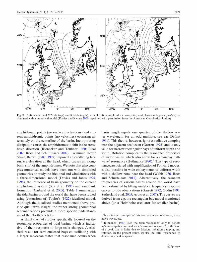
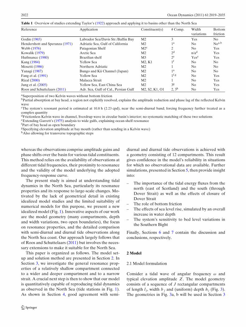
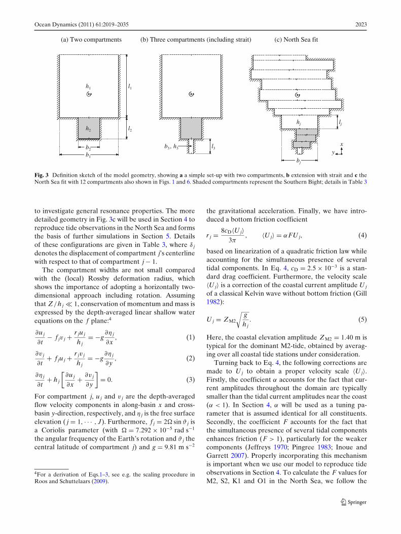
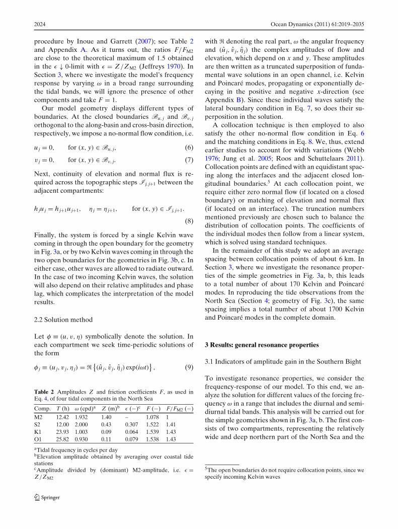
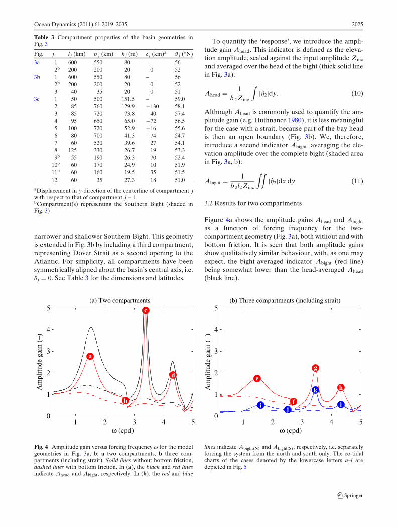
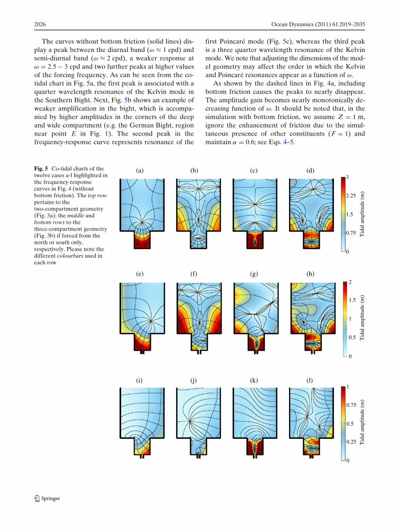
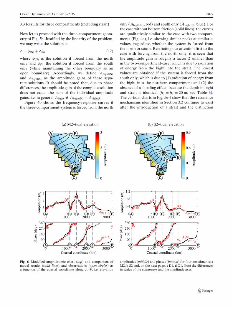
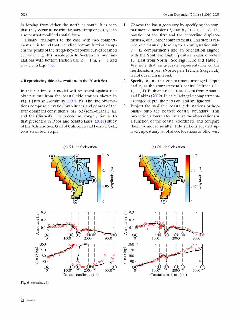
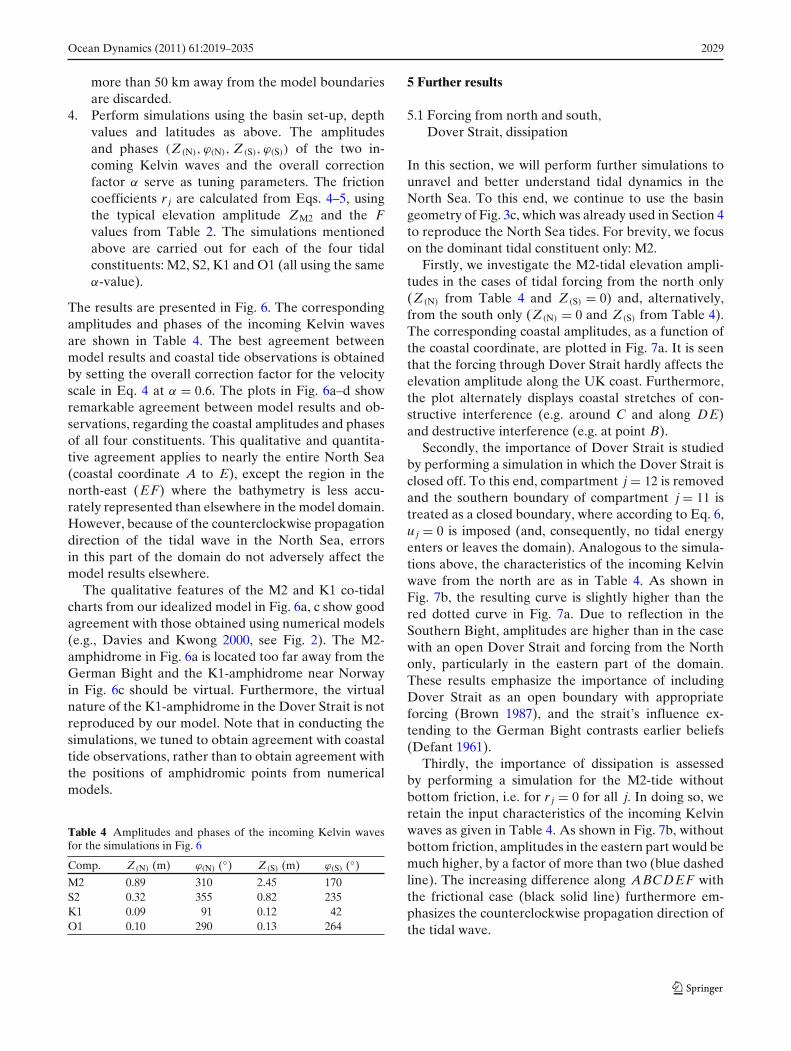
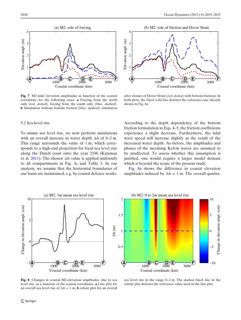
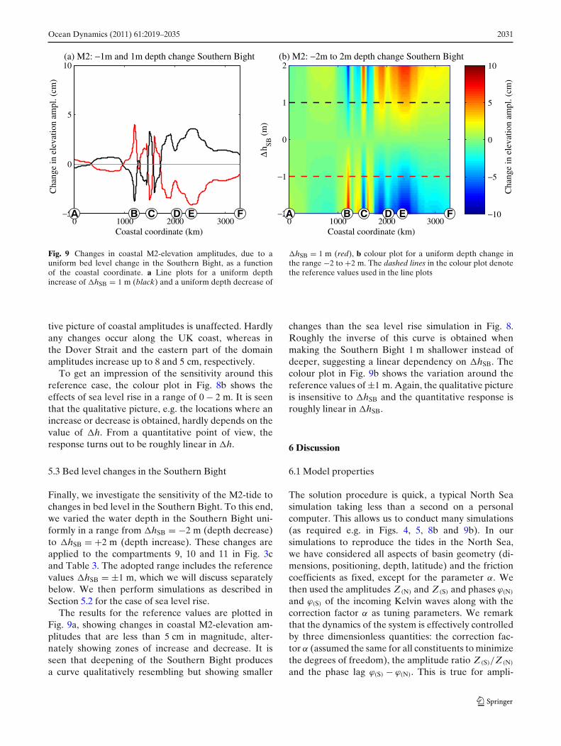